Quantum trajectories with incompatible decoherence channels
197
HAL Id: tel-03406048 https://tel.archives-ouvertes.fr/tel-03406048 Submitted on 27 Oct 2021 HAL is a multi-disciplinary open access archive for the deposit and dissemination of sci- entific research documents, whether they are pub- lished or not. The documents may come from teaching and research institutions in France or abroad, or from public or private research centers. L’archive ouverte pluridisciplinaire HAL, est destinée au dépôt et à la diffusion de documents scientifiques de niveau recherche, publiés ou non, émanant des établissements d’enseignement et de recherche français ou étrangers, des laboratoires publics ou privés. Quantum trajectories with incompatible decoherence channels Quentin Ficheux To cite this version: Quentin Ficheux. Quantum trajectories with incompatible decoherence channels. Physics [physics]. Université Paris sciences et lettres, 2018. English. NNT : 2018PSLEE088. tel-03406048
-
Upload
khangminh22 -
Category
Documents
-
view
1 -
download
0
Transcript of Quantum trajectories with incompatible decoherence channels
HAL Id: tel-03406048https://tel.archives-ouvertes.fr/tel-03406048
Submitted on 27 Oct 2021
HAL is a multi-disciplinary open accessarchive for the deposit and dissemination of sci-entific research documents, whether they are pub-lished or not. The documents may come fromteaching and research institutions in France orabroad, or from public or private research centers.
L’archive ouverte pluridisciplinaire HAL, estdestinée au dépôt et à la diffusion de documentsscientifiques de niveau recherche, publiés ou non,émanant des établissements d’enseignement et derecherche français ou étrangers, des laboratoirespublics ou privés.
Quantum trajectories with incompatible decoherencechannels
Quentin Ficheux
To cite this version:Quentin Ficheux. Quantum trajectories with incompatible decoherence channels. Physics [physics].Université Paris sciences et lettres, 2018. English. NNT : 2018PSLEE088. tel-03406048
THÈSE DE DOCTORAT
de l’Université de recherche Paris Sciences et Lettres PSL Research University
École Normale Supérieure
QUANTUM TRAJECTORIES WITH
INCOMPATIBLE DECOHERENCE CHANNELS
COMPOSITION DU JURY :
M. BERNARD Denis École Normale Supérieure, Membre du jury M. GOUGH John Aberystwyth University, Rapporteur M. JORDAN Andrew University of Rochester, Membre du jury M. LEEK Peter University of Oxford, Rapporteur M. ROCH Nicolas Institut Néel, Membre du jury M. HUARD Benjamin École Normale Supérieure de Lyon, Directeur de thèse M. LEGHTAS Zaki Mines ParisTech, Co-directeur de thèse
Soutenue par Quentin FICHEUX le 7 Décembre 2018 h
Ecole doctorale n°564 PHYSIQUE EN ÎLE DE FRANCE
Spécialité PHYSIQUE
Dirigée par Benjamin HUARD et codirigée par Zaki LEGHTAS

Quentin Ficheux, Quantum trajectories with incompatible decoherence channels.© october 2018

À celle qui se reconnaitra.


ABSTRACT
In contrast with its classical version, a quantum measurement necessarily disturbs thestate of the system. The projective measurement of a spin-1/2 in one direction maxi-mally randomizes the outcome of a following measurement along a perpendicular direc-tion. In this thesis, we discuss experiments on superconducting circuits that allow us toinvestigate this measurement back-action. In particular, we measure the dynamics ofa superconducting qubit whose three Bloch x, y and z components are simultaneouslyrecorded.
Two recent techniques are used to make these simultaneous recordings. The x andy components are obtained by measuring the two quadratures of the fluorescence fieldemitted by the qubit. Conversely, the z component is accessed by probing an off-resonant cavity dispersively coupled to the qubit. The frequency of the cavity dependson the energy of the qubit and the strength of this last measurement can be tunedfrom weak to strong in situ by varying the power of the probe. These observations areenabled by recent advances in ultra-low noise microwave amplification using Josephsoncircuits. This thesis details all these techniques, both theoretically and experimentally,and presents various unpublished additional results.
In the presence of the simultaneous measurements, we show that the state of thesystem diffuses inside the sphere of Bloch by following a random walk whose steps obeythe laws of the backaction of incompatible measurements. The associated quantumtrajectories follow a variety of dynamics ranging from diffusion to Zeno blockade. Theirpeculiar dynamics highlights the non-trivial interplay between the back-action of thetwo incompatible measurements. By conditioning the records to the outcome of a finalprojective measurement, we also measure the weak values of the components of thequbit state and demonstrate that they exceed the mean extremal values. The thesisdiscusses in detail the statistics of the obtained trajectories.
v

RÉSUMÉ
Au contraire de sa version classique, une mesure quantique perturbe nécessairementl’état du système. Ainsi, la mesure projective d’un spin-1/2 selon une direction rendparfaitement aléatoire le résultat d’une mesure successive de la composante du mêmespin le long d’un axe orthogonal. Dans cette thèse, nous discutons des expériencesbasées sur les circuits supraconducteurs qui permettent de mettre en évidence cetteaction en retour de la mesure. Nous mesurons en particulier la dynamique d’un qubitsupraconducteur dont on révèle simultanément les trois composantes de Bloch x, y etz.
Deux techniques récentes sont utilisées pour réaliser ces enregistrements simultanés.Les composantes x et y sont obtenues par la mesure des deux quadratures du champ defluorescence émis par le qubit. La composante z est quant à elle obtenue en sondant unecavité non résonante couplée de manière dispersive au qubit. La fréquence de la cavitédépend de l’énergie du qubit et la force de cette dernière mesure peut être ajustée in situen faisant varier la puissance de la sonde. Ces observations sont rendues possibles grâceaux avancées récentes dans l’amplification ultrabas bruit des signaux micro-onde grâceaux circuits Josephson. Cette thèse détaille toutes ces techniques à la fois théoriquementet expérimentalement et présente différents résultats annexes inédits.
En présence des mesures simultanées, nous montrons que l’état du système diffuse àl’intérieur de la sphère de Bloch en suivant une marche aléatoire dont les pas obéissentaux lois de l’action en retour de mesures incompatibles. Les trajectoires quantiquesassociées ont des dynamiques allant du régime diffusif au régime de blocage de Zénonsoulignant l’interaction non-triviale des actions en retours des deux mesures incom-patibles effectuées. En conditionnant les enregistrements aux résultats d’une mesureprojective finale, nous mesurons également les valeurs faibles des composantes de notrequbit et démontrons qu’elles dépassent les valeurs extrémales moyennes. La thèse dis-cute en détail de la statistique des trajectoires obtenues.
vi

Notre seul pouvoir véritable consiste à aider autrui.
— Tenzin Gyatso
REMERCIEMENTS
Mon nom est sur ce manuscrit mais ce travail de thèse est le fruit d’une intelligencecollective. Ma trajectoire professionnelle et personnelle est le résultat d’un grand nombred’interactions et de rencontres.
Certaines interactions sont de vraies forces motrices. Merci à Benjamin Huard dem’avoir fait confiance en me prenant dans le groupe. Benjamin est un chef prolifique,bienveillant et ambitieux. Il consacre beaucoup de temps à ses étudiants ce qui m’apermis de bénéficier de sa clairvoyance en physique et de ses talents de meneur. J’espèrepouvoir m’inspirer de sa réussite pour trouver ma voie dans le monde de la recherche.Notre équipe a été en constante évolution pendant ces trois années avec le départ deFrançois Mallet, l’arrivée de Zaki Leghtas et enfin notre départ à Lyon. Merci à Françoispour ses explications très précises et ses bonnes idées lorsque je découvrais le domainedes circuits supraconducteurs. Zaki est un physicien et une personne que j’admire. Jele remercie pour l’influence positive qu’il a sur moi. J’exprime toute ma gratitude àSébastien Jezouin qui m’a instruit au quotidien dès mon arrivée dans le groupe. Il m’aappris aussi bien les bases du métier de chercheur que les techniques les plus avancéesde ce manuscrit.
D’autres rencontres ont un effet stochastique dont le bilan est parfois productif etparfois égayant. L’atmosphère dans l’équipe est familiale et bon enfant. L’entraide, lafumisterie et l’autodérision sont toujours de mise. Merci Nathanaël Cottet avec qui j’aiéchangé bien plus que des frisbees et des avions en papier, Danijela Marković notregrande sœur de thèse qui a su nous supporter, Théau Peronnin l’éternel stagiaire de3eme accro au Coca-Cola et abonné aux allers-retours Paris-Lyon, Raphaël Lescanneque l’on a laissé à Paris mais qui nous manque, Jeremy Stevens pour qui "ça joue"toujours et qui assure, avec Antoine Essig, une relève d’un excellent niveau. Que ce soità la Montagne, au Mayflower, au Ninkasi ou au labo, cela a été et cela sera toujours unplaisir.
Afin de profiter au maximum de ces interactions, il est crucial d’évoluer dans un bonenvironnement. Le laboratoire Pierre Aigrain constitue un écosystème de choix pourfaire de la recherche. Merci à Michael Rosticher et José Palomo pour leurs conseils etleur bonne humeur dans la salle blanche. Merci à Takis Kontos dont la "funkytude"n’est plus à démontrer. Merci à l’équipe HQC et à tous les doctorants du LPA pourleur sympathie lors des pauses café. Merci à Jean-Marc Berroir, Jérôme Tignon et Jean-François Allemand qui sont des leaders sur qui nous pouvons compter. Le vendrediétait le jour des pizzas avec l’équipe Quantic de l’INRIA lors du "Tuesday LunchSeminar". Merci à Mazyar Mirrahimi, Alain Sarlette, Pierre Rouchon et leurs étudiantsqui maintiennent un très bon niveau dans le groupe. Merci à Olivier Andrieu pour lesnombreux footings au jardin du Luxembourg. Merci à l’équipe de mécanique de l’ENSParis qui nous a fourni les pièces nécessaires à nos expériences.
vii

Je remercie également tous les membres du laboratoire de physique de l’ENS deLyon qui nous a accueilli à bras ouverts. Il y règne une atmosphère très convivialeet stimulante propice à l’activité et la créativité. Merci à Thierry Dauxois qui est undirecteur de laboratoire modèle. Merci à Nadinne Clervaux et Fatiha Boucheneb qui ontété d’un support administratif aussi agréable qu’efficace. Merci aux doctorants du laboavec qui j’ai passé de très bons moments. Merci aux camarades de promotion retrouvés,Valentin, Charles-Edouard et Vincent. Merci aux services électroniques et mécaniquesqui nous ont beaucoup aidé lors de notre installation.
Le déménagement à Lyon a affecté ma vie personnelle en m’éloignant de Nolwenn.L’amour a su trouver un chemin au prix de long trajets qui étaient une bien maigrepeine comparée au plaisir de se retrouver. Merci à toi d’avoir toujours été là pour moi.
Je remercie mes parents, mon frère et ma famille qui ont su donner une excellentecondition initiale à ma trajectoire avec l’impulsion nécessaire pour aller toujours plusloin. Merci aux familles Morin et Laennec qui m’ont très rapidement considéré commeun des leurs. Merci à mes amis et colocataires qui ont vécu à mes côtés pendant cestrois années.
Merci enfin aux membres du jury qui ont accepté d’évaluer mon travail de thèse.
Lyon, octobre 2018 Quentin Ficheux
viii

CONTENTS
1 introduction 11.1 Background 11.2 Individual quantum systems 21.3 Decoherence and readout of a superconducting qubit 41.4 Quantum trajectories 61.5 Post-selected evolution 81.6 Outline 9
i measurement and control of superconducting circuits
2 introduction to superconducting circuits 132.1 Circuit quantum electrodynamics 13
2.1.1 Introduction 132.1.2 Quantum LC oscillator 142.1.3 Open quantum systems 172.1.4 Cavity coupled to two transmission lines 18
2.2 Transmon qubit 212.2.1 Black-box quantization of a transmon embedded in a cavity 242.2.2 Finite element simulation - Energy participation ratios 28
2.3 Open system dynamics of a qubit 292.3.1 Qubits 292.3.2 Entropy of a qubit 312.3.3 Decoherence mechanisms 31
2.4 Conclusion 34
3 readout of a superconducting qubit 353.1 Measuring a quantum system 36
3.1.1 Generalized measurement 363.1.2 Continuous measurement 38
3.2 Dispersive readout 393.2.1 Homodyne detection of the cavity field 393.2.2 AC stark shift and measurement induced dephasing 43
3.3 Measurement of fluorescence 453.3.1 Heterodyne detection of the fluorescence of a qubit 453.3.2 Destructive and QND measurements 47
3.4 Full quantum tomography 483.4.1 Direct access to the Bloch vector 483.4.2 Tomography of a qubit undergoing Rabi oscillations 503.4.3 Comparing the fidelities of a weak and projective quantum to-
mography 523.5 Conclusion 53
4 qutrits 554.1 Introduction 55
ix
contents
4.2 Preparation of an arbitrary quantum superposition of three levels 554.3 Projective tomography of a three-level system 56
4.3.1 From the measurement output to the density matrix 574.3.2 Representation of the density matrix of a qutrit 58
4.4 Quadrature plane calibration and temperature measurement 594.4.1 Calibration of the IQ plane 594.4.2 Direct temperature measurement 61
4.5 Open-system dynamics of a three-level atom 624.5.1 Lindblad equation 624.5.2 Energy relaxation 634.5.3 Ramsey experiments 64
4.6 Continuous measurement of a three-level system 654.6.1 Dispersive measurement of a qutrit 664.6.2 Quantum jumps between three levels 67
4.7 Conclusion 69
5 microwave amplifiers 715.1 Introduction 715.2 Quantum parametric amplification 71
5.2.1 Phase preserving amplification 715.2.2 Phase sensitive amplification 73
5.3 Josephson parametric amplifier 735.3.1 Different JPAs and different pumping schemes 755.3.2 Amplification 795.3.3 Frequency tunability 80
5.4 Josephson parametric converter 815.4.1 Josephson ring modulator 815.4.2 Amplification mode 835.4.3 Flux tunability 86
5.5 Travelling wave parametric amplifier 865.5.1 Phase matching condition 865.5.2 Amplification performance 87
5.6 Figures of merit of amplifiers 895.6.1 Amplifying setup 895.6.2 Gain 905.6.3 Quantum efficiencies 915.6.4 Dynamical bandwidth 915.6.5 Static bandwidth 925.6.6 Dynamical range 925.6.7 Comparison between two detection chains and a JTWPA 92
5.7 Conclusion 93
ii measurement back-action
6 quantum trajectories 976.1 Quantum back-action of measurement 98
6.1.1 Kraus operators formulation 98
x
contents
6.1.2 Dispersive interaction 1006.1.3 Measurement along the orthogonal quadrature 1026.1.4 Fluorescence signal 105
6.2 Quantum trajectories 1076.2.1 Repeated Kraus map and Markov chain 1076.2.2 The stochastic master equation 1086.2.3 From measurement records to quantum trajectories 1096.2.4 Validation by an independent tomography 1116.2.5 Parameter estimation 113
6.3 Trajectories statistics 1156.3.1 Different regimes 1156.3.2 Zeno dynamics - Interplay between detectors 1176.3.3 Rabi oscillations 1196.3.4 Exploration of several regimes 121
6.4 Diffusion of quantum trajectories 1236.4.1 Introduction 1236.4.2 Fokker-Planck equation 1236.4.3 Impact of the efficiencies on the statistics 1256.4.4 Convection velocity 1276.4.5 Diffusion tensor 1286.4.6 Dimensionality of the diffusion 1286.4.7 Diffusivity 1296.4.8 An Heisenberg-like inequality for pure states 130
6.5 Conclusion 132
7 post-selected quantum trajectories 1337.1 Past quantum state 134
7.1.1 Prediction and retrodiction 1347.1.2 Continuous time dynamics 136
7.2 Pre and post-selected trajectories 1387.2.1 Time symmetric Rabi evolution 1387.2.2 "Anomalous" weak values 1417.2.3 Influence of the post-selection 143
7.3 Conclusion 145
iii appendix
a transmon coupled to a transmission line 149a.1 Classical equation of motions 149
a.1.1 Dynamics of the system 149a.1.2 Asymptotic expansion in 152
a.2 Quantum description 152a.3 Conclusion 154
b experimental techniques 155b.1 Fabrication 155
b.1.1 Fabrication of JPA and JPC 155b.1.2 3D transmons 160
xi

contents
b.1.3 2D CPW chips 161b.2 Measurement setup 162
iv bibliography
bibliography 167
xii

L I ST OF F IGURES
Figure 2.1 LC oscillator 15Figure 2.2 Open quantum system 19Figure 2.3 Transmission and reflection coefficients 20Figure 2.4 Josephson junction 22Figure 2.5 SEM image of a 2D transmon 23Figure 2.6 Black-box quantization 25Figure 2.7 Black-box quantization for a transmon embedded in a cavity 27Figure 2.8 Bloch sphere representation of a qubit state 30Figure 2.9 Decoherence channels of a qubit 33Figure 3.1 Dispersive measurement of a qubit by homodyne detection 40Figure 3.2 Single-shot dispersive readout of a transmon qubit by homodyne
measurement 42Figure 3.3 Tomography of a superconducting qubit by dispersive readout 43Figure 3.4 Measurement induced dephasing on a transmon qubit 44Figure 3.5 Heterodyne detection of the fluorescence emitted by an atom 46Figure 3.6 Complete detection setup 49Figure 3.7 Rabi oscillations monitored by a continuous quantum tomogra-
phy 51Figure 4.1 Readout of a qutrit 58Figure 4.2 Qutrit state preparation 58Figure 4.3 Relaxation of a ‘GEF’ state 59Figure 4.4 Calibration of the IQ plane for the dispersive measurement of
a qutrit 60Figure 4.5 Temperature measurement of a qubit by projective measure-
ment 62Figure 4.6 Energy relaxation of a qutrit 64Figure 4.7 Ramsey type experiments on a qutrit 65Figure 4.8 Single-shot readout of a ‘GEF’ state 66Figure 4.9 Jumps between three levels of a qutrit 68Figure 5.1 Phase preserving and phase sensitive amplification 72Figure 5.2 Josephson parametric amplifier (JPA) device 73Figure 5.3 Reflection coefficient of the JPA 75Figure 5.4 JPA pumping schemes 76Figure 5.5 Gain and flux dependence of the JPA 80Figure 5.6 Josephson ring modulator (JRM) 82Figure 5.7 Gain and flux dependence of a Josephon parametric converter
(JPC) 84Figure 5.8 JPC device 84Figure 5.9 Josephson traveling parametric amplifier (JTWPA) 88Figure 5.10 Amplifying chain composed of low noise amplifiers 89
xiii

Figure 6.1 Integrable quantity for the detection of the cavity field 101Figure 6.2 Integrable quantity for iz measurement 104Figure 6.3 Integrable quantity for fluorescence measurement 106Figure 6.4 Autocorrelations of the filtered measurement records 110Figure 6.5 Measurement records and a single quantum trajectory 111Figure 6.6 Validation of the quantum trajectories by independent tomog-
raphy 112Figure 6.7 Determination of the quantum efficiencies by checking the va-
lidity of the quantum trajectories 114Figure 6.8 Direct averaging of the measurement records in the Zeno and
Rabi oscillation regimes 116Figure 6.9 Distribution of quantum trajectories in the Zeno regime 118Figure 6.10 Time evolution of the probability distribution of quantum tra-
jectories in the Rabi oscillation regimes 120Figure 6.11 Javascript application to visualize quantum trajectories 121Figure 6.12 Panel of all reachable regimes 122Figure 6.13 Comparison between experimental and simulated statistics 125Figure 6.14 Simulated statistics for increasing efficiencies 126Figure 6.15 Convection velocity field 127Figure 6.16 Diffusivity of incompatible measurement channels 130Figure 7.1 Density matrix and effect matrix in discrete times 135Figure 7.2 Continuous prediction and retrodiction of a quantum state 137Figure 7.3 Pre and post-selected Rabi oscillations exhibiting time symme-
try 139Figure 7.4 Pre and post-selected Rabi oscillation exhibiting ‘anomalous’
weak values 142Figure 7.5 Influence of the post-selection on an average trace 143Figure A.1 Transmon coupled to a transmission line 150Figure B.1 Dolan bridge technique to evaporate Josephson junction 156Figure B.2 Comparison of the MIBK/IPA and H2O/IPA development 158Figure B.3 Evaporation of Aluminum and wafer probing 159Figure B.4 Inside of a dilution refrigerator 163Figure B.5 Schematics of the wiring for the quantum trajectories experi-
ment 164
L I ST OF TABLES
Table 4.1 List of pulses to prepare an arbitrary superposition of threequantum states 56
Table 4.2 Jump operators for a qutrit 63Table 5.1 Comparison of the different pumping schemes for a JPA 78Table B.1 List of devices 160
xiv
1INTRODUCTION
1.1 background
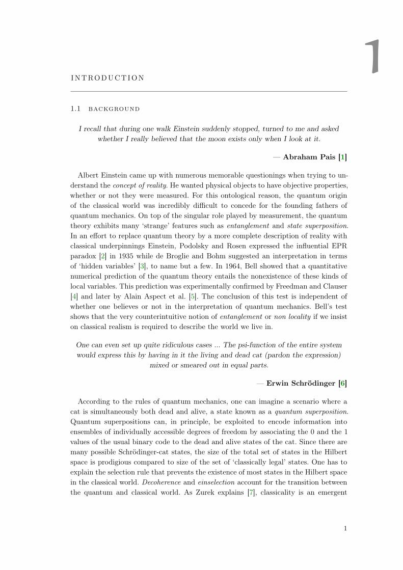
I recall that during one walk Einstein suddenly stopped, turned to me and asked
whether I really believed that the moon exists only when I look at it.
— Abraham Pais [1]
Albert Einstein came up with numerous memorable questionings when trying to un-derstand the concept of reality. He wanted physical objects to have objective properties,whether or not they were measured. For this ontological reason, the quantum originof the classical world was incredibly difficult to concede for the founding fathers ofquantum mechanics. On top of the singular role played by measurement, the quantumtheory exhibits many ‘strange’ features such as entanglement and state superposition.In an effort to replace quantum theory by a more complete description of reality withclassical underpinnings Einstein, Podolsky and Rosen expressed the influential EPRparadox [2] in 1935 while de Broglie and Bohm suggested an interpretation in termsof ‘hidden variables’ [3], to name but a few. In 1964, Bell showed that a quantitativenumerical prediction of the quantum theory entails the nonexistence of these kinds oflocal variables. This prediction was experimentally confirmed by Freedman and Clauser[4] and later by Alain Aspect et al. [5]. The conclusion of this test is independent ofwhether one believes or not in the interpretation of quantum mechanics. Bell’s testshows that the very counterintuitive notion of entanglement or non locality if we insiston classical realism is required to describe the world we live in.
One can even set up quite ridiculous cases ... The psi-function of the entire system
would express this by having in it the living and dead cat (pardon the expression)
mixed or smeared out in equal parts.
— Erwin Schrödinger [6]
According to the rules of quantum mechanics, one can imagine a scenario where acat is simultaneously both dead and alive, a state known as a quantum superposition.Quantum superpositions can, in principle, be exploited to encode information intoensembles of individually accessible degrees of freedom by associating the 0 and the 1values of the usual binary code to the dead and alive states of the cat. Since there aremany possible Schrödinger-cat states, the size of the total set of states in the Hilbertspace is prodigious compared to size of the set of ‘classically legal’ states. One has toexplain the selection rule that prevents the existence of most states in the Hilbert spacein the classical world. Decoherence and einselection account for the transition betweenthe quantum and classical world. As Zurek explains [7], classicality is an emergent
1

introduction
property induced in a system by its interaction with the environment. During theinteraction, the system transmits information into its environment through quantumchannels. In these conditions, the information on the quantum state is lost in the manydegrees of freedom of the bath except for a preferred set of pointer states (or classicalstates) that survive the interaction. Since information is exchanged, decoherence canbe seen as a continuous observation of the system by its environment.
Observations not only disturb what has to be measured, they produce it. We compel
to assume a definite position. . . We ourselves produce the results of measurements.
— Pascual Jordan [8]
As Pascual Jordan puts it, information is acquired by an observer only when measure-ment records are produced by observation. The state of a system is encoded in a densitymatrix which refers to an observer’s knowledge about the system. More precisely, thedensity matrix contains the probability of outcomes of any future measurements that anobserver can perform on the system conditioned on her knowledge about the system atthat time. Every time a measurement is performed, the observer updates his knowledgeon the state of the system to take into account the measurement record, this effect isknown as measurement back-action. To go back to Einstein’s questioning, in general wecannot answer deterministically if the moon was there or not without the interventionof an observer. Different observers with different knowledge may assign simultaneouslydifferent density matrices to a same system revealing the observer-dependent characterof the quantum state. One of the main results of this thesis is to demonstrate this factexperimentally with continuous measurement.
Shut up and calculate!
— David Mermin
David Mermin beautifully epitomized the general attitude adopted by most physi-cists toward the philosophical questions raised by quantum theory. In this thesis, wesuggest the alternative approach "Shut up and contemplate!" [9] by providing textbookexperimental observations of measurement and decoherence ‘in action’ on a quantumsystem. Directly accessible macroscopic systems, on which one makes up one’s intuition,never display entanglement, state superposition or measurement back-action. The ‘in-triguing’ aspects of quantum mechanics are more easily observed in systems made of alimited number of well-defined quantum degrees of freedom.
1.2 individual quantum systems
... it is fair to state that we are not experimenting with single particles, any more
than we can raise Ichthyosauria in the zoo.
— Erwin Schrödinger [10]
2

1.2 individual quantum systems
As a matter of fact, experiments involving single particles such as electrons, atoms orphotons are nowadays routinely realized all over the world. A lot of different technologiesare found in the zoo of experiments involving only a small number of quantum degreesof freedom including trapped ions [11], cavity quantum electrodynamics [12], circuitquantum electrodynamics [13], quantum dots [14], cavity optomechanics [15], etc ...
In this thesis, we manipulate quantum devices constructed from superconductingelectrical circuits [16, 17, 18] (introduced in chapter 2). These circuits are composed ofa large number of microscopic particles that exhibits a very simple set of macroscopiccollective degrees of freedom. They form resonators and transmission lines that can becombined together in a modular manner. The insertion of non linear components suchas Josephson junctions enables us to mimic the non linearity introduced by matterin quantum electrodynamics. However, in contrast with real atoms, superconductingdevice parameters can be tuned during their fabrication by design.
We use one particular kind of superconducting device dubbed the transmon [19,20] (section 2.2). At a temperature of a few tens of mK, the transmon behaves as anartificial atom with independently addressable levels. The first two levels |gi and |eiare usually used as a qubit (two-dimensional Hilbert space) but there is no restrictionto use it as qutrit (three dimensions) as in chapter 4 by addressing the third level |fior even as qudit (N dimensions) (see Fig. 1.1) to encode more information.
a. b.
Figure 1.1: a. Bloch sphere representation of a quantum state = 12 (1+xx + yy + zz) of a
qubit. The ground state is the south pole z = 1 and the excited state is the north
pole z = +1. Only the poles of the sphere correspond to ‘classically legal’ states
while all the other states correspond to quantum superpositions of classical states.
b. Experimental density matrix of the superposed state | i (|gi+ i |ei+ |fi)/p3
of a qutrit (section 4.2).
These circuits provide an excellent test-bed for the Gedanken experiments envisionedby the founding father of quantum mechanics and quantum optics. Quantum circuitsare also among the many promising candidate platforms that could lead to the adventof a universal quantum computer [13, 21].
3

introduction
1.3 decoherence and readout of a superconducting qubit
The electromagnetic environment of the transmon is controlled by placing it into acavity (see Fig. 1.2). The macroscopic size of the artificial atom allows a coupling to thecavity much larger than the rate of the dissipation processes [22] enabling us to explorethe light-matter interaction at the most fundamental level. The qubit is manipulatedwith microwave photons at the frequency of the qubit fq sent at the input port of thesystem. The electromagnetic environment induces decoherence on the qubit either byextracting information via photons temporarily stored inside the cavity (section 3.2.2),or by collecting photon spontaneously emitted by the artificial atom or even by excitingthe qubit. This last mechanism can be neglected in our systems by making sure thatthe environment is almost in a vacuum state.
Figure 1.2: We place an artificial atom inside a cavity that is connected to the rest of the elec-
trical circuit via two ports. We monitor the spontaneous emission of the transmon
(in green) at fq while concurrently probing the state of the cavity (in purple) at fdthat is coupled to the qubit. The photons are amplified with a Josephson parametric
amplifier (at the frequency of the cavity) and a Josephson parametric converter (at
the frequency of the qubit). Qubit rotations are performed by sending a resonant
drive at the input.
We said earlier that decoherence can be seen as the action of an observer on thesystem (chapter 3). Let us be that observer. We monitor the decoherence channel asso-ciated with the energy relaxation of the qubit by measuring the complex amplitude ofthe outgoing field in green on Fig. 1.2. We obtain information on the real and imaginaryparts of the lowering operator of the qubit = (x iy)/2. Therefore, the associatedcontinuous measurement records u(t) and v(t) reveal respectively the information onthe x and y components of the qubit [23, 24, 25]. This detection is called fluorescencemeasurement (section 3.3).
When the qubit-cavity detuning is much larger than their interaction rate, the naturaldipolar interaction between the qubit and the cavity couples the z component of thequbit to the average number of excitations stored inside the cavity. Probing the state ofthe cavity leads to a continuous measurement record w(t) which yields the z componentof the qubit [26, 27, 28, 29]. This very standard readout procedure is known as dispersivemeasurement (section 3.2).
By raw averaging the measurement records u(t), v(t) and w(t), genuine quantumeffects caused by measurement back-action vanish. In this case, monitoring both de-coherence channels of the qubit is equivalent to imaging the average evolution of the
4
1.3 decoherence and readout of a superconducting qubit
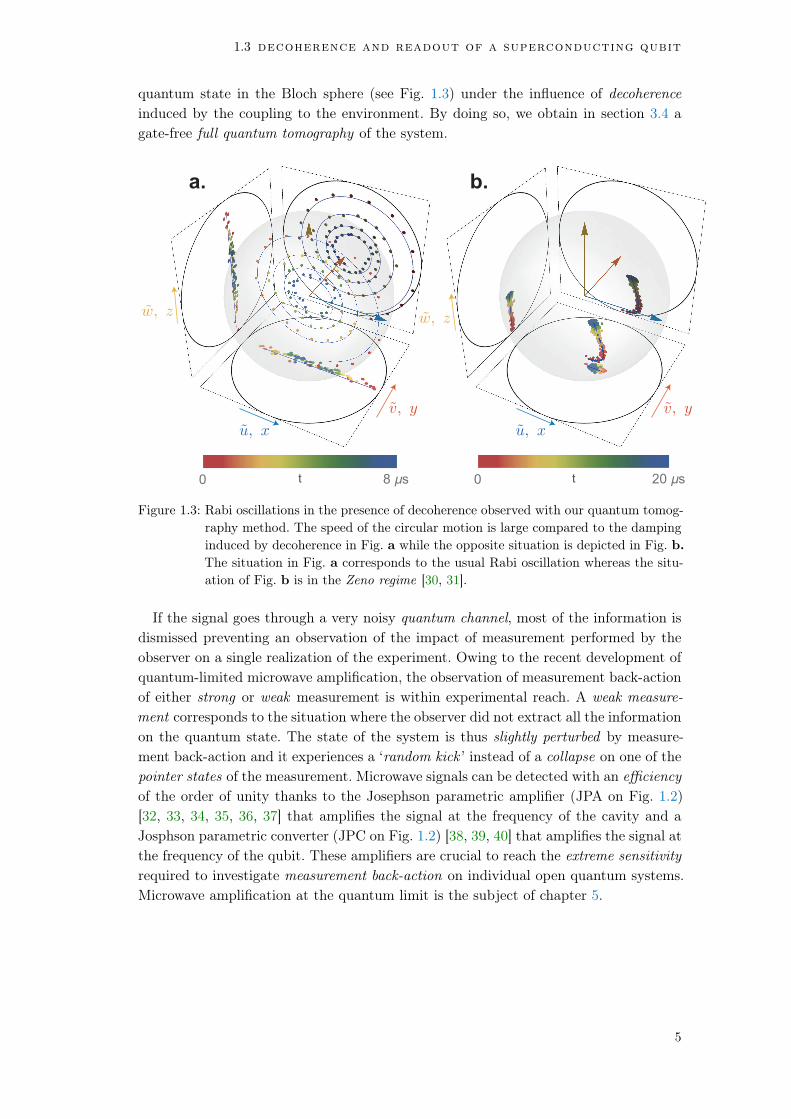
quantum state in the Bloch sphere (see Fig. 1.3) under the influence of decoherenceinduced by the coupling to the environment. By doing so, we obtain in section 3.4 agate-free full quantum tomography of the system.
a. b.
t t
Figure 1.3: Rabi oscillations in the presence of decoherence observed with our quantum tomog-
raphy method. The speed of the circular motion is large compared to the damping
induced by decoherence in Fig. a while the opposite situation is depicted in Fig. b.
The situation in Fig. a corresponds to the usual Rabi oscillation whereas the situ-
ation of Fig. b is in the Zeno regime [30, 31].
If the signal goes through a very noisy quantum channel, most of the information isdismissed preventing an observation of the impact of measurement performed by theobserver on a single realization of the experiment. Owing to the recent development ofquantum-limited microwave amplification, the observation of measurement back-actionof either strong or weak measurement is within experimental reach. A weak measure-ment corresponds to the situation where the observer did not extract all the informationon the quantum state. The state of the system is thus slightly perturbed by measure-ment back-action and it experiences a ‘random kick ’ instead of a collapse on one of thepointer states of the measurement. Microwave signals can be detected with an efficiencyof the order of unity thanks to the Josephson parametric amplifier (JPA on Fig. 1.2)[32, 33, 34, 35, 36, 37] that amplifies the signal at the frequency of the cavity and aJosphson parametric converter (JPC on Fig. 1.2) [38, 39, 40] that amplifies the signal atthe frequency of the qubit. These amplifiers are crucial to reach the extreme sensitivityrequired to investigate measurement back-action on individual open quantum systems.Microwave amplification at the quantum limit is the subject of chapter 5.
5

introduction
1.4 quantum trajectories
When continuously monitoring a qubit, its quantum state undergoes a non trivialstochastic evolution but the experimentalist can use the measurement outcomes toreconstruct a posteriori the evolution of the system. The density matrix of the systemis updated at each time step conditioned on the random measurement outcome to takeinto account the succession of non-projective ‘kicks’ caused by the measurement. The re-sulting path in the Hilbert space is called a quantum trajectory (see Fig. 1.4) [41, 42, 43,44, 45, 46, 26, 27, 47, 48, 28, 23, 29, 49, 25]. Chapter 6 contains an in-depth descriptionof fundamental concepts and experimental implementation of quantum trajectories.
1 2 3 4 5-10
-5
0
5
10a. b.
Figure 1.4: A 5 µs-long tracking of a quantum state. a. Raw (not normalized) measurement
records u(t) (blue), v(t) (red) and w(t) (yellow) as a function of time for one re-
alization of the experiment. b. Bloch sphere representation of the reconstructed
quantum trajectory.
The inherent back-action of a quantum measurement is better discussed by repre-senting distributions of states at a given time (see Fig. 1.5) as the randomness of themeasurement back-action spreads apart quantum states corresponding to different real-izations of the experiment. We can isolate the contribution of dispersive measurement(Fig. 1.5 a b c) [26, 27] from the contribution of the energy relaxation (Fig. 1.5 d e f)[23, 25] or we can combine the effect of both measurements at the same time (Fig. 1.5g h i) by collecting the records of one or the two detectors. While both measurementslead to the same average trajectory, their back-action differ. The uniqueness of percep-tion of the three observers has its roots in the records stored in the observer’s memoryand it leads to the distinct statistics of Fig. 1.5. We prove in section 6.2.4 that everyobservers can safely use their density matrices to predict the results of an independenttomography.
The asymmetry of Fig. 1.5 g reveals the incompatibility of the dispersive measure-ment and fluorescence measurement (section 6.3.2). Monitoring dynamics of a systemundergoing incompatible measurements provides a test of quantum foundations by ex-posing the subtle interplay between different back-action at the single quantum systemlevel. The possibility to achieve simultaneous incompatible measurements was only very
6

1.4 quantum trajectories
a. b. c.
d. e. f.
i.h.g.
dispersive measurement
fluorescence measurement
dispersive and fluorescence measurement
# trajectories1 10 100 1000
Figure 1.5: Impact of the type of detector on the distribution of quantum states in the Zeno
regime of Fig. 1.3 b. a,b,c Marginal distribution in the xy (a), xz (b) and yz
(c) planes of the Bloch sphere of the qubit states τ corresponding to 1.5 millions of
measurement records w(t) at the cavity frequency only. The information about
u(t), v(t) is here discarded. The boundary of the Bloch sphere is represented as a
black circle and the average quantum trajectory as a solid line. d,e,f Case where the
states are conditioned on fluorescence records u(t), v(t) instead while discarding
the information on w(t). g,h,i Case where the states are conditioned on both
fluorescence and dispersive measurement records u(t), v(t), w(t).
7

introduction
recently demonstrated by Hacohen-Gourgy et al. [49] in the case of a qubit with two de-phasing channels. Jordan and Bütikker [50] proposed such an experiment theoreticallyin 2005. By monitoring both decoherence channels, we take the place of the environ-ment in this experiment and we reveal the knowledge that only the bath acquires inmost experiments.
The quantum state diffuses inside the Bloch sphere, which is reminiscent of theBrownian motion [51] of a particle inside a colloid as explained in section 6.4. In thiscase, the measurement back-action plays the role of the Langevin force. The probabilitydistribution of quantum trajectories obeys the celebrated Fokker-Planck equation. Wegain insight into the physics of the diffusion of the quantum trajectories by analyzingthe different terms of the Fokker-Planck equation. We find that our experiment is thefirst observation of a genuine 3D diffusion inside the Bloch sphere (section 6.4.6) andwe explain the deep link between diffusion and back-action. The incompatibility ofour measurement is encoded in a persistant diffusion enforced by a Heinsenberg-likeinequality on the diffusivity of quantum states (section 6.4.8).
1.5 post-selected evolution
In the 50s, von Neumann and Bohm [52, 53] suggested that the irreversible collapse ofa wave packet of the state of a system under the influence of measurement introducesa fundamental time asymmetry at the microscopic level. The measurement back-actionwas thus thought of as a time asymmetric element in quantum theory. Nevertheless, thesymmetry of the rules of quantum mechanics is fully restored when specifying both theinitial state and the final state of a closed system. The symmetric role of preparationor pre-selection and post-selection was enlightened by Aharonov et al. in 1964 [54].While the density matrix t is the quantum state of the system conditioned on thepast measurement records, the effect matrix Et [55, 56, 57, 58] is the quantum stateconditioned on the information available in the future (chapter 7). Taking into accountthe forward and backward estimation of the quantum state at the same time provides aso-called past quantum state that encapsulates all the information available from pastand future measurements (section 7.1).
preparation post-selection
prediction retrodiction
Figure 1.6: The state of the system can be predicted conditioned on past measurement records
using the density matrix t or rectrodicted, a posteriori, conditioned on the future
measurement records by unravelling the effect matrix Et. The past quantum state
(t, Et) uses the complete measurement records to give an estimate of the distribu-
tion of any measurement performed on the system at time t.
8

1.6 outline
In the presence of both preparation and post-selection, the measured expectation val-ues of the signal can spread outside of the eigenvalue range defined by the correspondingobservable. These anomalous values were called weak values [59, 60] and they can, inprinciple, reach arbitrarily large values. In this thesis, we present the results of an ex-periment illustrating this fact. By combining preparation and post-selection, the Blochvector imaged with our direct quantum tomography method exceeds the boundary ofthe unit sphere [61, 62, 63, 64] in section 7.2.2.
1.6 outline
This thesis is organized as follows. Chapter 2 gives an introduction to the field ofsuperconducting circuits. It aims at bridging the gap from the condensed matter aspectof superconducting circuits to the open quantum mechanics description of qubits andharmonic oscillators. In chapter 3 we describe a novel gate-free tomography method.The x and y components of the qubit are obtained by measuring the two quadratures ofthe fluorescence field emitted by the artificial atom while the z component is accessedby probing an off-resonant cavity dispersively coupled to the qubit. The experimentalistis not restricted to the first two levels of the transmon. We demonstrate in chapter 4the coherent control and readout of a transmon qutrit. We give a general explanationof the most commonly used near quantum limited amplifiers in the microwave rangein chapter 5. These amplifiers are instrumental to observe the partial collapse of thedensity matrix under the influence of weak measurement. Measurement back-action andquantum trajectories are at the heart of chapter 6. We investigate the case of multiplesimultaneous observers monitoring incompatible operators on the same quantum bit.Impressively, the random walk of the state of the system in the Bloch sphere can bestudied with the tools of classical diffusion physics. Finally chapter 7 investigates thebehavior of post-selected quantum trajectories revealing weak values of our detectionsignals that exceed the boundary of the unit sphere.
The White Rabbit put on his spectacles. “Where shall I begin, please your Majesty ?”
he asked. “ Begin at the beginning,” the King said, gravely, “ and go on till you come
to the end : then stop.”
— Lewis Carroll, Alice’s Adventures in Wonderland
9


Part I
MEASUREMENT AND CONTROL OF SUPERCONDUCTING
CIRCUITS


2INTRODUCTION TO SUPERCONDUCTING CIRCUITS
The goal of this first part is to give an up-to-date introduction to the field of super-conducting circuits from an experimentalist perspective while focusing on the devicesthat are used in this thesis work. The first chapter will focus on the transmon qubit,which is the most widespread qubit in the superconducting circuit community. A lot ofother types of qubits have very promising performances but they are not the subject ofthis thesis. The second chapter is dedicated to the readout of superconducting qubitswith a particular emphasis on dispersive and fluorescence readout that are crucial tothe second part of this thesis. The third chapter is dedicated to three-level systems.Most applications of superconducting circuits rely on quantum operations on two-levelsystems while transmons offer many more levels that are individually addressable. In-creasing the size of the Hilbert space for quantum operations or quantum algorithmsopens up new perspectives for quantum physics and quantum information processing.The fourth chapter is dedicated to pumped microwave circuits and more specifically tolinear microwave amplifiers. Three kinds of amplifiers were used in this work and a non-exhaustive review is given on the current state-of-the-art of microwave amplification atthe quantum level.
In this first chapter, we will introduce the transmon as an elementary unit instrumen-tal to circuit QED. We will start by introducing quantum circuits from the solid-statephysics perspective and then we combine it with the universal quantum mechanicsdescription valid for a wide range of platforms dealing with single quantum systems.
2.1 circuit quantum electrodynamics
2.1.1 Introduction
The goal of cavity quantum electrodynamics (CQED) is to study the properties of light(photons) coupled to matter (electrons, atoms, ...). This field has led to numerousground-breaking experiments [12, 65] well described in books and reviews such as Ex-ploring the quantum by Serge Haroche and Jean-Michel Raimond [66]. Subsequently, anew branch of this field emerged in 1999 with the invention of the first superconduct-ing qubit [17] later followed by the demonstration of strong coupling regime betweena transmon and a resonator [22] and was dubbed circuit QED. This first section isdedicated to the quantum optics of microwave circuits with superconducting artificialatoms.
A first striking property of these circuits is that they are macroscopic quantum sys-tems. While they contain a large number of microscopic particles, they host macroscopicdegrees of freedom that behave quantum-mechanically. Secondly, their properties arenot set by fundamental constants like the Rydberg energy. They are engineered at willby design with the technology of microelectronic chips. Lastly, a truly remarkable level
13
introduction to superconducting circuits
of control was achieved in these systems thanks to the exponential growth of coherencetimes of these devices known as Schoelkopf’s Law [13]. The system used throughout thisthesis is the transmon1, which is nowadays the most commonly used superconductingqubit. This qubit was originally envisioned to be coupled to a 2D resonator connectedto a transmission line [19] but it can also be embedded into a 3D electromagnetic orinto a lumped mode [67] in order to straightforwardly increase the quality factor of theLC resonator.
Transmons are usually made of a Josephson junction shunted by a large capacitance[20] and the circuit is shielded and anchored to the base plate of a dilution refrigeratorat about 20 mK so that the energy of the thermal fluctuations is much smaller thanthe energy quantum at a few GHz ~! kBT .
Another important thing to mention about superconducting circuits is that it is oneof the many candidate platforms that could lead to the advent of a universal quantumcomputer thanks to quantum error correction [68, 69]. A lot of landmarks were achievedsuch as the implementation of multi qubit algorithms [70] or gate fidelities sufficientfor error correction [71] and few small uncorrected quantum processors are alreadyavailable online but the race is still ongoing.
2.1.2 Quantum LC oscillator
A quantum LC oscillator is the simplest circuit element that can be built with capac-itors and inductors [73, 74] as depicted in Fig. 2.1 a. In practice, the dynamics of acavity mode is modeled by a harmonic oscillator. The most commonly used resonatorsin circuit QED are 3D rectangular cavities machined out of aluminum (Fig. 2.1 b),3D coaxial /4 cavities (Fig. 2.1 c) and /2 coplanar-wave-guide (CPW) resonators(Fig. 2.1 d). There are no resistors in the circuit representation because the cavities aremade out of superconducting materials that ensure that the supercurrent flows withnegligible dissipation in the circuit. Losses will be introduced as a perturbation. In thecase of a rectangular cavity of dimensions lx, ly, lz, the limit conditions impose thatthe resonant frequency of the TEmnl and TMmnl modes are given by [75]
fnml =c
2
sm
lx
2
+
n
ly
2
+
l
lz
2
(2.1)
where the indices n, m, l refer to the number of anti-nodes in standing wave pattern inthe x, y, z directions. A cavity with dimensions (lx, ly, lz) = (26.526.59.6) mm3 hasa first TE110 mode at f1,1,0 = 8 GHz. Similarly, a coaxial /4 cavity has a fundamentalresonance frequency f0 ' 4.25 GHz for l = 20 mm [76] well separated from its first har-monic frequency f1 = 3f0 = 12.75 GHz. Finally, /2 CPW resonators are planar trans-mission lines terminated by two open circuits loads. The two terminations are sufficientto create a standing wave as in a Fabry-Pérot cavity and a l = 20 mm resonator willhave a fundamental mode at f0 = 8.5 GHz. The first harmonic is f1 = 2f0 = 17 GHz.
1 The original name comes from transmission-line shunted plasma oscillation qubit [19].
14
2.1 circuit quantum electrodynamics
a. b.
c. d. e.
wg
λ/2
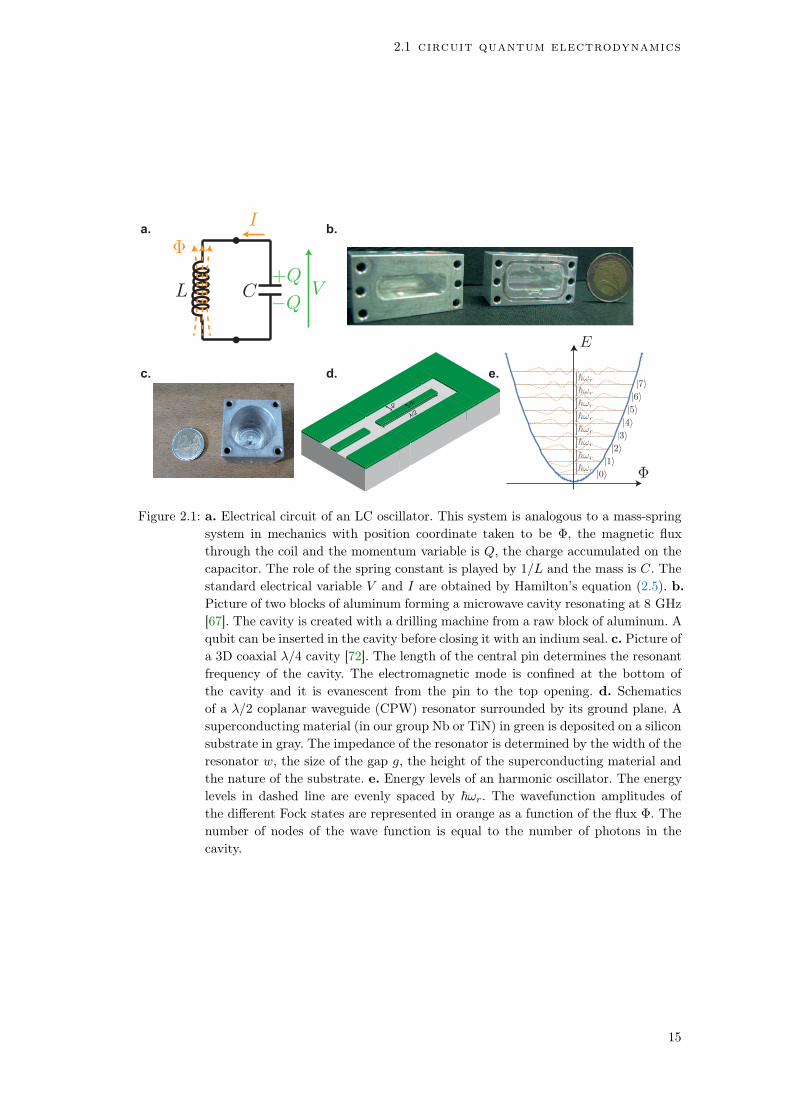
Figure 2.1: a. Electrical circuit of an LC oscillator. This system is analogous to a mass-spring
system in mechanics with position coordinate taken to be Φ, the magnetic flux
through the coil and the momentum variable is Q, the charge accumulated on the
capacitor. The role of the spring constant is played by 1/L and the mass is C. The
standard electrical variable V and I are obtained by Hamilton’s equation (2.5). b.
Picture of two blocks of aluminum forming a microwave cavity resonating at 8 GHz
[67]. The cavity is created with a drilling machine from a raw block of aluminum. A
qubit can be inserted in the cavity before closing it with an indium seal. c. Picture of
a 3D coaxial /4 cavity [72]. The length of the central pin determines the resonant
frequency of the cavity. The electromagnetic mode is confined at the bottom of
the cavity and it is evanescent from the pin to the top opening. d. Schematics
of a /2 coplanar waveguide (CPW) resonator surrounded by its ground plane. A
superconducting material (in our group Nb or TiN) in green is deposited on a silicon
substrate in gray. The impedance of the resonator is determined by the width of the
resonator w, the size of the gap g, the height of the superconducting material and
the nature of the substrate. e. Energy levels of an harmonic oscillator. The energy
levels in dashed line are evenly spaced by ~!r. The wavefunction amplitudes of
the different Fock states are represented in orange as a function of the flux Φ. The
number of nodes of the wave function is equal to the number of photons in the
cavity.
15

introduction to superconducting circuits
The Lagrangian of the classical system is readily written as the difference of thepotential energy stored in the capacitor and the kinetic energy stored in the inductor
L =Q2
2C Φ
2
2L(2.2)
by defining the flux threading the coil Φ and the charge on the capacitor Q accordingto
8
>>><
>>>:
Φ =
Z t
1V (t0)dt0
Q =
Z t
1I(t0)dt0
. (2.3)
And the Hamiltonian can be written
H = QΦ L =Φ2
2L+
Q2
2C. (2.4)
Hamilton’s equations of motion give us the current crossing the inductor and thevoltage applied across the leads of the capacitor
8
>><
>>:
Φ =@H
@Q=
Q
C= V
Q = @H@Φ
= Φ
L= I
(2.5)
Remarkably the whole complexity of the system containing an enormous number ofelectrons boils down to a system with a single position degree of freedom. We choosethe flux threading the coil Φ as the position coordinate. The system is simply analogousto a spring with mass2 C, spring constant 1/L and momentum Q. The two variablesΦ and Q can be promoted to quantum operators Φ and Q that obey the canonicalcommutation relation
[Φ, Q] = i~. (2.6)
The Hamiltonian now reads
H =Φ2
2L+
Q2
2C. (2.7)
We can diagonalize it in the usual form
H = ~!r
a†a+1
2
(2.8)
in terms of the ladder operators8
>><
>>:
a =1p
2~L!rΦ+ i
1p2~C!r
Q
a† =1p
2~L!rΦ i
1p2~C!r
Q
, (2.9)
2 Note that it is also possible to choose the charge accumulated on the capacitor as the position coordinatebut with a ‘mass’ L and ‘spring constant’ 1/C.
16
2.1 circuit quantum electrodynamics
with !r = 1/pLC. And the creation and annihilation operators obey the usual bosonic
relation [a, a†] = 1. The number operator n = a†a gives the number of quanta in themode that we dub photons. We can think of these quanta as collective excitations ofboth the electrical field and the Cooper pairs inside the materials3.
The energy spectrum of the harmonic oscillator is represented in Fig 2.1e. The energylevels of the harmonic oscillator are evenly spaced as predicted from (2.8). Sending acold enough classical microwave radiation at energy ~!r inevitably populates all thelevels of the Hilbert space with a Poisson distribution leaving the cavity in a coherentstate. In order to prepare other states, one needs to couple the oscillator to a non linearelement or to perform postselection or non-Gaussian measurements. This will be therole of the Josephson junction in the following.
The charge and flux operators can then be expressed as(
Φ = ΦZPF(a+ a†)
Q = iQZPF(a a†), (2.10)
where the zero-point fluctuations are defined as a function of the characteristic impedance
of the resonator Z =p
L/C by QZPF =q
~
2Z and ΦZPF =q
~Z2 . Notice that the
Heisenberg minimal uncertainty product is given by QZPFΦZPF = ~
2 .Equation (2.5) allows to estimate the zero-point voltage fluctuations of a cavity mode
in the ground state
VZPF QZPF
C !r
r
~
2Z 0.4 µV (2.11)
with !r = 2 8 GHz and Z = 100 Ω.
2.1.3 Open quantum systems
In practice our microwave circuits are open quantum systems and the above groundworkhas to be completed by connecting the harmonic oscillator to the rest of the circuitryto enable coherent control and measurement of the system. The dynamics of an opensystem of Hamiltonian H is governed by the Lindblad equation
dtdt
= i
~[H, t] +
X
k
Dk(t)dt, (2.12)
where t is the density matrix of the cavity at time t, Dk(t) = LktL†k 1
2tL†kLk
12L
†kLkt is the dissipation super-operator and Lk are the jump operators. Each index
k is associated to an irreversible quantum channel and the effect of the interactionbetween the bath and the system is encoded in Lk.
This very general differential equation describes the decoherence of an open quantumsystem by extending the Schrödinger equation to Markovian open systems, that is,
3 Note that usually physicists rigorously speak about photons only as excitations of a free propagatingelectromagnetic mode but our denomination is legitimized by the fact that the stationary photons thatwe defined above can fully be converted into propagating excitations of a transmission line whose limitconditions can be continuously impedance matched to infinity.
17

introduction to superconducting circuits
local in time [77]. Local in time means that t+dt must be entirely determined by t.Dissipation originates from the fact that energy and information can flow from thesystem to the bath however if this is a two-way process, information can also flow backin the system and give rise to a non-Markovian evolution of the system since we needto know the value of at earlier times.
In order to derive the Lindblad Eq. (2.12) the following hypotheses are required [66]
• We usually deal with Eq. (2.12) by dividing the time into ‘slices’ of duration dt
and every evolution t from time t to t+ dt is incremental. This ‘coarse-grained’description of the first order differential Eq. (2.12) screens out high frequencycomponent of the dynamics with ! 1/dt. We thus perceive the dynamics ofthe studied system through a filter and this description will be accurate only fordt TH where TH is the typical time scale of evolution of the observables of due to unitary evolutions or damping processes.
• The environment must be a ‘sink’. We assume that this large system has a greatnumber of degrees of freedom (represented by the collection of discrete electro-magnetic modes in Fig. 2.2 b) and that the dynamics of the bath does not impactthe dynamics of the system. This amounts to neglect the memory effects of thebath (also called reservoir in statistical physics). Mathematically we denote byE the time scale of the fluctuations and correlations of the environment. Theinequality E dt is required to ensure that the environment is amnesic at thescale dt. We thus renounce to the microscopic description of fluctuations muchfaster than dt.
• There is no notion of quantum measurement in the derivation of Eq. (2.12). Con-tinuous quantum measurement will be introduced in Chapter 3 and the dynamicsof the quantum state will be predicted by the stochastic master equation in chap-ter 6.
In the case of a cavity losing photons ‘one-by-one’ via a coupling to a transmissionline, only one jump operator is non zero L =
pa where is the coupling rate to the
transmission line. We will see the jump operators associated to a qubit in a followingsection and for any given system that satisfies the above-listed conditions, there existsa set of jump operators describing the decoherence of the system.
2.1.4 Cavity coupled to two transmission lines
In this thesis, we used two-port cavities with jump operators L1 =p1a and L2 =p
2a. The input-output relation (see appendix A)
pia = aiin + aiout (2.13)
relates the input and output propagating modes of the transmission line to the station-ary mode a of the device. In the case of 3D resonators, the value of the coupling isdetermined by the length of the pins of the SMA connectors mounted on the cavity,while the coupling is given by a planar capacitance in the case of 2D resonators. In our
18
2.1 circuit quantum electrodynamics
a. b. c.
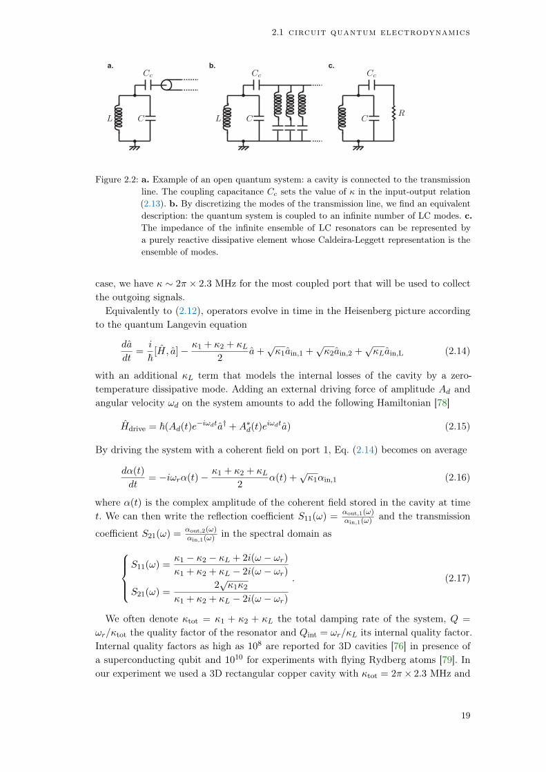
Figure 2.2: a. Example of an open quantum system: a cavity is connected to the transmission
line. The coupling capacitance Cc sets the value of in the input-output relation
(2.13). b. By discretizing the modes of the transmission line, we find an equivalent
description: the quantum system is coupled to an infinite number of LC modes. c.
The impedance of the infinite ensemble of LC resonators can be represented by
a purely reactive dissipative element whose Caldeira-Leggett representation is the
ensemble of modes.
case, we have 2 2.3 MHz for the most coupled port that will be used to collectthe outgoing signals.
Equivalently to (2.12), operators evolve in time in the Heisenberg picture accordingto the quantum Langevin equation
da
dt=
i
~[H, a] 1 + 2 + L
2a+
p1ain,1 +
p2ain,2 +
pLain,L (2.14)
with an additional L term that models the internal losses of the cavity by a zero-temperature dissipative mode. Adding an external driving force of amplitude Ad andangular velocity !d on the system amounts to add the following Hamiltonian [78]
Hdrive = ~(Ad(t)ei!dta† +A
d(t)ei!dta) (2.15)
By driving the system with a coherent field on port 1, Eq. (2.14) becomes on average
d↵(t)
dt= i!r↵(t)
1 + 2 + L
2↵(t) +
p1↵in,1 (2.16)
where ↵(t) is the complex amplitude of the coherent field stored in the cavity at timet. We can then write the reflection coefficient S11(!) =
↵out,1(!)↵in,1(!)
and the transmission
coefficient S21(!) =↵out,2(!)↵in,1(!)
in the spectral domain as
8
>><
>>:
S11(!) =1 2 L + 2i(! !r)
1 + 2 + L 2i(! !r)
S21(!) =2p12
1 + 2 + L 2i(! !r)
. (2.17)
We often denote tot = 1 + 2 + L the total damping rate of the system, Q =
!r/tot the quality factor of the resonator and Qint = !r/L its internal quality factor.Internal quality factors as high as 108 are reported for 3D cavities [76] in presence ofa superconducting qubit and 1010 for experiments with flying Rydberg atoms [79]. Inour experiment we used a 3D rectangular copper cavity with tot = 2 2.3 MHz and
19

introduction to superconducting circuits
a total quality factor of 500 dominated by the coupling to one of the transmissionline to enhance photon collection by the so-called Purcell effect explained below.
From Eq. (2.17), we can see that the transmission profile is always a Lorentzian inamplitude accompanied with a phase shift (see Fig 2.3). The width of Lorentzianand the phase shift is always given by tot. In reflection on port 1, three regimes areobserved.
• The over-coupled regime is defined by 1 L + 2. In this regime the lossesare negligible so in reflection |S11(!)| = 1 and a 2 phase shift is observed (bluecurve in Fig 2.3).
• The critical coupling corresponds to 1 = L + 2. In this regime a phase shiftis observed in reflection while the amplitude vanishes at resonance (green curvein Fig 2.3).
• The under-coupled regime corresponds to L+2 1. A bigger dip in amplitudeis observed in reflection due to the important losses with a phase shift (redcurve in Fig 2.3).
-1.0 -0.5 0.0 0.5 1.0-1.0-0.50.0
0.5
1.0
Re[S11]
Im[S 11]
0.0 0.1 0.2 0.3 0.4 0.5
-0.2-0.10.0
0.1
0.2
Re[S21]
Im[S 21]
a. b. c.
d. e. f.
-0.2 -0.1 0.0 0.1 0.2
-40-30-20-10
(ω-ωr)/2π (GHz)
20Log[S 21]
(dB)
-0.2 -0.1 0.0 0.1 0.2
- π2
- π4
0
π4
π2
(ω-ωr)/2π (GHz)
Arg[S 21]
(rad)
-0.2 -0.1 0.0 0.1 0.2-10-8-6-4-20
(ω-ωr)/2π (GHz)
20Log[S 11]
(dB)
-0.2 -0.1 0.0 0.1 0.2-π- π2
0
π2
π
(ω-ωr)/2π (GHz)
Arg[S 11]
(rad)
Figure 2.3: Reflection (a, b and c) and transmission (d, e and f) signal through the cavity
given by Eq. (2.17) for 2 = 2 100 kHz, L = 2 1 MHz and various 1(indicated by color). The distinct over-coupled (blue line), critical (green curve)
and under-coupled (red curve) regimes are observed in the reflected signal whereas
the transmitted signals are all Lorentzian resonances.
20

2.2 transmon qubit
2.2 transmon qubit
Now that we know how to deal with open quantum systems, we need to add a nonlinear element to complete the cQED toolbox. The transmon is an artificial atom madeof a Josephson junction connected to two superconducting islands. In our case thealuminum/alumina/aluminum junction is typically 250 200 nm and the associatedtunnel resistance at room temperature of the order of 2 to 8 kΩ (see appendix B). Thecoupling Hamiltonian associated to the coherent tunneling of a Cooper pair throughthe barrier reads
Htunneling = EJ
2
+1X
N=1(|Ni hN + 1|+ |N + 1i hN |) (2.18)
where EJ is a macroscopic parameter, which is proportional to the DC conductanceGn of the junction in the normal state, which can be adjusted during the fabricationprocess and to the superconducting gap ∆ of the material EJ = ∆Gn
h8e2
. The state|Ni corresponds to exactly N Cooper pairs having passed through the junction.
We can define a new ‘plane wave’ basis
|'i =+1X
N=1eiN' |Ni . (2.19)
The number ' can be thought of as an angle since '! '+2 leaves |'i unaffected. Thevariable ' corresponds to the superconducting phase difference across the junction andthe Josephson relation relates to the electromagnetic flux by ' = Φ
'0(mod 2) with the
reduced flux quantum '0 =~
2e . The tunneling Hamiltonian (2.18) is formally a hoppingHamiltonian in a 1D tight-binding model, so we get the usual cosine dispersion relation
Htunneling |'i = EJ cos(') |'i . (2.20)
On top of this tunneling energy, one has to consider the charging energy. The po-tential energy associated with the transfer of a single electron is EC = e2
2C with C thecapacitance between the two superconducting islands so the energy operator associatedwith the transfer of a Cooper pair is four times larger. We obtain the Cooper Pair Box(CPB) Hamiltonian [80]
H = 4EC(N Ng)2 EJ
\cos('). (2.21)
where we added Ng called the dimensionless gate charge. It represents either the effect ofa voltage applied across the junction or a junction asymmetry that breaks the symmetrybetween positive and negative charge transfer [73]. We define the number operatorN =
P+1N=0N |Ni hN |. The number operator N has integer eigenvalues whereas Ng is
a continuous variable. The Hamiltonian (2.21) is formally identical to the Hamiltonianof a ‘quantum rotor’ in a gravity field with the charging energy playing the role of‘moment of inertia’ and the Josephson energy as the torque produced by gravity.
Unfortunately, the gate charge uncontrollably fluctuates and this is what limited theinterest of the CPB as a qubit [17, 81]. However when EJ/EC 50 or above, the energy
21
introduction to superconducting circuits
a.
b. c.
Tappin
g A
mplitu
de
max
min
Josephson
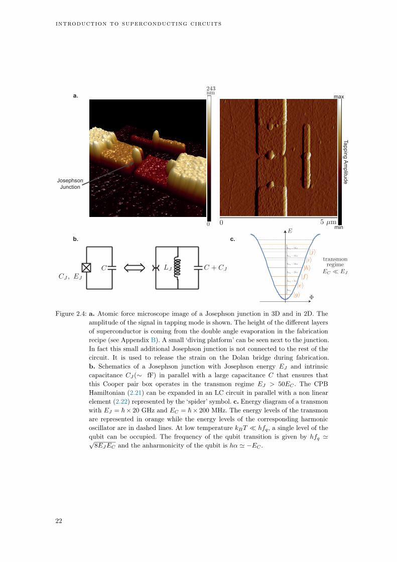
Junction
Figure 2.4: a. Atomic force microscope image of a Josephson junction in 3D and in 2D. The
amplitude of the signal in tapping mode is shown. The height of the different layers
of superconductor is coming from the double angle evaporation in the fabrication
recipe (see Appendix B). A small ‘diving platform’ can be seen next to the junction.
In fact this small additional Josephson junction is not connected to the rest of the
circuit. It is used to release the strain on the Dolan bridge during fabrication.
b. Schematics of a Josephson junction with Josephson energy EJ and intrinsic
capacitance CJ( fF) in parallel with a large capacitance C that ensures that
this Cooper pair box operates in the transmon regime EJ > 50EC . The CPB
Hamiltonian (2.21) can be expanded in an LC circuit in parallel with a non linear
element (2.22) represented by the ‘spider’ symbol. c. Energy diagram of a transmon
with EJ = ~ 20 GHz and EC = ~ 200 MHz. The energy levels of the transmon
are represented in orange while the energy levels of the corresponding harmonic
oscillator are in dashed lines. At low temperature kBT hfq, a single level of the
qubit can be occupied. The frequency of the qubit transition is given by hfq 'p8EJEC and the anharmonicity of the qubit is h↵ ' EC .
22

2.2 transmon qubit
spectrum of the CPB becomes almost independent of Ng, this is the so-called transmonregime [19, 20]. In our design, we make sure to operate in this regime by shunting thejunction by a large enough capacitance that is obtained by connecting the junctionto large enough pads (see Fig. 2.5). From the Hamiltonian (2.21), we see that in thisregime eigenstates have a well defined phase Φ and a large Q uncertainty in charge Q.
b.
c.
a.
d. e.
2D
arc
hit
ec
ture
3D
arc
hit
ec
ture
Figure 2.5: a. Scanning electron microscope image under an angle of a 2D transmon embed-
ded in a niobium CPW circuit. The Josephson junction made out of aluminum is
connected to two large pads forming a large capacitance that lowers the charging
energy EC = ~ e2
2C ' ~ 234 MHz. b. and c. Zooms on the Josephson junction de-
posited by double angle evaporation with the Dolan bridge technique (see appendix
B). d. 3D aluminum cavity with a sapphire chip. The chip is gripped on its two
edges between two blocks of aluminum to ensure that the substrate is thermalized.
We measured EJ = ~ 20.588 GHz and EC = ~ 174 MHz for this chip so we are
deeply in the tranmson regime. e. SEM image of the Josephson junction of the 3D
transmon device, which is very similar to the one on silicon in Fig. c.
By reording the terms in (2.21), we obtain
H =
4EC(N Ng)2 +
1
2EJ '
2
EJ
| z
HHO
EJ
\cos(') +'2
2 1
| z
HNL
(2.22)
23

introduction to superconducting circuits
where HHO is the Hamiltonian of the harmonic oscillator HHO = hfq(a†a + 1/2) at
frequency fq = 1h
p8EJEC , which is of the order of 5 GHz in our systems. In the
limit ' 1, the purely non-linear term reads
HNL = EJ(\cos(') + '2/2 1) ' EJ('4/4! '6/6! + '8/8! + ...). (2.23)
This term is symbolized by the spider element in Fig. 2.4 and is responsible for thenon evenly spaced distribution of the energy levels. This anharmonicity is crucial toselectively manipulate a limited number of levels and effectively truncate the Hilbertspace. Specifically, the first two levels |gi and |ei are used as a two-level system or qubitthroughout this thesis and in the third chapter we additionally used the third level |fito work with a qutrit.
The basics features of the transmon circuit (Fig. 2.4b) were explained in this sec-tion without taking into consideration the cavity. Introducing it at this stage becomesquite technical since the geometry of the transmon and cavity modes are affected anddistorted by one another to become dressed states, which both inherit some non lin-earity of the junction. The complexity increases further by including the harmonics ofthe cavity. We rather derive an effective Hamiltonian with the Black-box quantizationmethod.
2.2.1 Black-box quantization of a transmon embedded in a cavity
2.2.1.1 General theory with a single junction
Typical circuits used in our experiments have more degrees of freedom than a simpleharmonic oscillator and all the complexity of the system can be captured in a ‘black box’.The black box quantization method was originally introduced by Nigg et al. [82]. Gener-alizations of this method have been proposed by Solgun et. al. [83] and Malekakhlagh et.al. [84] to model more complex environment but we restrict the discussion to the Fosterdecomposition of the environment. Its principle relies on solving the linearized problemand treat the non linearity perturbatively. In the case of a linear circuit, knowing theimpedance Z(!) or admittance Y (!) = Z1(!) of a dipole black box connected as afunction of frequency completely characterizes its quantum properties.
We start by decomposing the impedance seen by the junction into M RLC-oscillatorsin series4 Z(!) =
PMp=1(j!Cp+
1j!Lp
+ 1Rp
)1 (Fig. 2.6). First, neglecting the dissipationassociated to the Rp elements, the Hamiltonian of the linear system reads [85]
Hlinear =
MX
p=1
~!p(a†pap + 1/2) (2.24)
with !p = 1/p
LpCp (for weak dissipation i.e. RP p
LP /Cp). This Foster decompo-sition is equivalent to diagonalizing coupled modes into M uncoupled hybrid or dressedmodes which are collective excitations of the linear circuit. The ladder operators of
each mode p are defined as ap =q
12~Zp
Φp + iq
Zp
2~Qp with Zp =pLp/Cp. We obtain
4 It is important to understand that usually the circuit elements drawn in electrical circuits have nophysical counter part in the actual device.
24

2.2 transmon qubit
a. b. c.
Figure 2.6: a. Schematics of a Josephson junction coupled to an arbitrary linear circuit dubbed
‘cavity modes’ for the transmon. b. The Josephson element is replaced by a purely
non linear element (spider symbol) the linear inductance LJ and capacitance Cj of
the junction together with the cavity modes are encapsulated in an impedance Z(!)
seen by the spider element. c. The impedance is replaced by its pole decomposition
(Foster-equivalent) Z(!) =PM
p=1(j!Cp + 1jωLp
+ 1Rp
)1. We also introduce the
fluxes Φp used in the text.
the expression of the flux across the junction Φ =PM
p=1 Φp that can be reinjected inthe non linear Hamiltonian (2.23). By restricting ourselves to the first non linear term,we obtain
HNL =X
p
∆pnp +1
2
X
pp0
~pp0 npn0p (2.25)
with the excitation number operator np = a†pap of mode p. The Lamb-shift of mode p
is ∆p = e2
2LJ(Zp
P
p0 Zp0 Z2p/2) expressing a frequency ‘renormalization’ due to the
presence of the other modes. The expressions of the self-Kerr pp and cross-Kerr pp0
constants are given by8
><
>:
~pp = Lp
LJ
CkCp
EC = Z2p
CkLJ
EC
~pp0 = 2pppp0p0
(2.26)
where Ck is the capacitance shunting the junction. Lastly, the finite width of the reso-nances are given by the imaginary part of the zeros of the admittance Y (!) = Z1 ofthe Black-box. The quality factor of mode p is given by
Qp =!p
2
Im[Y 0(!p)]
Re[Y (!p)]. (2.27)
Similarly to the non-linearity, dissipation is spread over all effective modes. This methodcan be extended to multiple non linearities coupled to an arbitrary black box but itrequires heavier equations [82]. We will know apply it to the case of a transmon coupledto a cavity.
2.2.1.2 Application to the transmon
For a transmon inside a cavity, the qubit and cavity are treated as electromagneticmodes on equal footing and then we account for the weak non linearity of the Joseph-son potential perturbatively5. As depicted above, there is no clear separation between
5 Note that this method is applicable to transmon qubits because they exhibit a weak anharmonicitythat allow the perturbative treatment.
25

introduction to superconducting circuits
the qubit and the cavity in this model and one mode with a strong (resp. weak) anhar-monicity is called qubit-like (resp. cavity like). Mathematically speaking the qubit-likemode has a much higher impedance seen by the junction Zq Zp for all p. By restrict-ing ourselves to one cavity mode, we obtain a total Hamiltonian similar with a nonlinear part given by Eq. (2.25)
HBBQ = ~!qa†qaq + ~!ca
†cac ~a†caca
†qaq ~
↵
2a†2q a2q + ~
K
2a†2c a2c (2.28)
where !q and !c are the dressed qubit and cavity frequencies, aq and ac are the anni-hilation operators of the qubit-like and cavity-like modes. The non-linear terms reads
8
>>>>>><
>>>>>>:
↵ = qq/~ =EC
~(anharmonicity of the transmon)
= 2qc/~ = 2↵ g
∆
2(cavity pull)
K = cc/~ = Zc
Zq
2 EC
~(self Kerr of the cavity mode)
. (2.29)
In practice the anharmonicity of the cavity K is negligible because Zq Zc and inour system |K| 2 40 kHz so we will neglect this term in the rest of the thesis.The interaction strength is given by cavity pull6 as a function of the dipolar couplingconstant g between the artificial atom and the electrical field and the detuning ∆ =
|!q!c| [86]. The cavity pull is of the order of a few MHz in our experiments and it maybe enhanced by increasing the length of the antenna to obtain a greater dipole moment.The anharmonicity of the transmon ↵ is of the order of ↵ 2 100 200 MHz. Itsvalue is controlled by the charging energy which is set by the antenna area.
The cavity mode is connected to a resistor (Fig. 2.7) modeling the coupling to anexternal transmission line. Photons leak out of the cavity on a time scale 1 andEq. (2.27) predicts a finite quality factor Qq for the qubit-like mode and thus a finitedecay rate known as Purcell rate Γ1,Purcell = !q/Qq. We obtain the Purcell decay ratethat limits the lifetime of the transmon
Γ1,Purcell = 2Re[Y 0(!q)]
Im[Y 0(!q)]'
g2
∆2. (2.30)
In practice with typical values g/2 = 290 MHz, /2 = 2.3 MHz and ∆/2 =
2.4 GHz, we obtain Γ1,Purcell = (4.7 µs)1 which is much higher than the experimen-tal value. This known discrepancy [86] could be due to one of the approximations ofthe model and it is nonetheless possible to get a good approximation of Γ1, Purcell bysimulating directly the admittance seen by the junction with finite-element simulations.However we make sure that the relaxation time of the qubit is limited by Purcell effectin this thesis to be able to collect a significant part of the spontaneous emission in theoutput line (see chapter 3).
6 The cavity-pull of the transmon is reduced by a factor 1/∆ compared to a Jaynes-Cummings hamilto-nian due to higher levels.
26
2.2 transmon qubit
a. b. c..
.
.
.
.
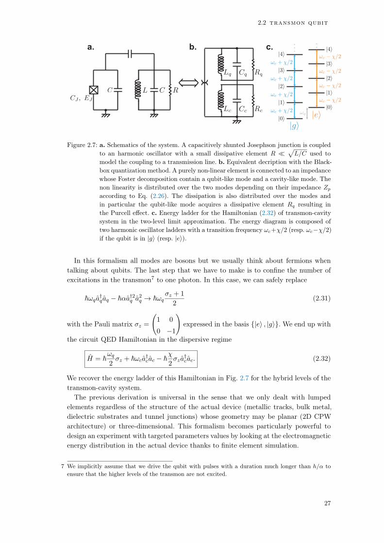
Figure 2.7: a. Schematics of the system. A capacitively shunted Josephson junction is coupled
to an harmonic oscillator with a small dissipative element R p
L/C used to
model the coupling to a transmission line. b. Equivalent decription with the Black-
box quantization method. A purely non-linear element is connected to an impedance
whose Foster decomposition contain a qubit-like mode and a cavity-like mode. The
non linearity is distributed over the two modes depending on their impedance Zp
according to Eq. (2.26). The dissipation is also distributed over the modes and
in particular the qubit-like mode acquires a dissipative element Rq resulting in
the Purcell effect. c. Energy ladder for the Hamiltonian (2.32) of transmon-cavity
system in the two-level limit approximation. The energy diagram is composed of
two harmonic oscillator ladders with a transition frequency !c+/2 (resp. !c/2)if the qubit is in |gi (resp. |ei).
In this formalism all modes are bosons but we usually think about fermions whentalking about qubits. The last step that we have to make is to confine the number ofexcitations in the transmon7 to one photon. In this case, we can safely replace
~!qa†qaq ~↵a†2q a2q ! ~!q
z + 1
2(2.31)
with the Pauli matrix z =
1 0
0 1
!
expressed in the basis |ei , |gi. We end up with
the circuit QED Hamiltonian in the dispersive regime
H = ~!q
2z + ~!ca
†cac ~
2za
†cac. (2.32)
We recover the energy ladder of this Hamiltonian in Fig. 2.7 for the hybrid levels of thetransmon-cavity system.
The previous derivation is universal in the sense that we only dealt with lumpedelements regardless of the structure of the actual device (metallic tracks, bulk metal,dielectric substrates and tunnel junctions) whose geometry may be planar (2D CPWarchitecture) or three-dimensional. This formalism becomes particularly powerful todesign an experiment with targeted parameters values by looking at the electromagneticenergy distribution in the actual device thanks to finite element simulation.
7 We implicitly assume that we drive the qubit with pulses with a duration much longer than h/α toensure that the higher levels of the transmon are not excited.
27

introduction to superconducting circuits
2.2.2 Finite element simulation - Energy participation ratios
In order to predict the values of the frequencies !p in (2.24) and ’s in (2.26), weperform classical finite element simulation of our devices8. We replace the Josephsonelement by a lumped9 electromagnetic element of inductance LJ and capacitance10 Cj
and the solver extracts the electromagnetic eigenmodes of the linear problem (2.24).The frequency of the eigenmode p is !p and even its quality factor Qp (see Eq. (2.27))can be predicted by introducing losses in the simulation.
The solver gives the stationary electric and magnetic eigenfields ~Em(~r) and ~Hm(~r)
of mode m where ~r indicates the spatial coordinates. The total electromagnetic en-ergy of the system breaks down in the sum of its inductive energy Einductive andits capacitive energy Ecapacitive. The inductive energy originates from the magneticfields and from the kinetic energy stored in the lumped linear inductance of the junc-tion Einductive = Emag fields + Ekinetic whereas the capacitive energy is solely storedin the electrical fields Ecapacitive = Eelec fields. When a stationary mode m is excitedon resonance the total energy equilibrates between inductive and capacitive energyEcapacitive = Einductive because of the equipartition theorem.
We introduce the energy participation ratios of the junction to the mode m as thefraction of inductive energy stored in the junction when exciting mode m
pm =EkineticEinductive
m
=equipartition
Eelec fields Emag fields
Eelec fields(2.33)
where the electromagnetic energies are computed as [87]8
>><
>>:
Eelec fields =1
2
Z
d3~r
~E(~r).(~r). ~E(~r)
Emag fields =1
2
Z
d3~r
~H(~r).µ(~r). ~H(~r) (2.34)
where (resp. µ) denotes the electric-permittivity tensor (resp. magnetic-permeabilitytensor).
Interestingly the list of participation ratio pm is sufficient to characterize the non-linearity of a multi-mode circuit hosting one Josephson junction. It is easy to show thatthey are real numbers between 0 and 1 and that they sum up to one
PMm=1 pm = 1.
We typically obtain participation ratios of the order of 0.9 for qubit-like modes and 0.1 for cavity-like modes. It is possible to show that11 the impedance of mode m seenby the junction is simply Zm = !m
EJpm and from Eq. (2.26) we obtain the non linear
terms of the Hamiltonian as a function of the participation ratios8
>><
>>:
mm = ~!2mp2m8EJ
mn = ~!m!n
4EJpmpn (for n 6= m)
(2.35)
8 These simulations are performed using HFSS or Sonnet.9 The lumped approximation is justified by the fact the size of the junction hundreds nm is very small
compared to the wavelength cm of the electromagnetic modes.10 In practice, we forget about this capacitance because it is negligible in the transmon regime.11 Zlatko Minev et al. in preparation.
28

2.3 open system dynamics of a qubit
In practice, we use an open-source package pyEPR12 developed by Zlatko Minevand Zaki Leghtas which automates the energy participation ratio approach with HFSS.The package allows to compute the non linear couplings between electromagnetic modeswith more than one junction and at an arbitrary order in the expansion of the cosinepotential (2.23). This package was tested in the design of several experiments [88, 89,90] and it fills the need for a simple and systematic method to predict the non-linearinteraction of the increasingly complex and diverse architecture of circuit QED.
2.3 open system dynamics of a qubit
Now that we understand the transmon, we can forget about the solid-state descriptionof the device and replace it with the quantum physics representation of a two statessystem called qubit or spin system. The qubit is the quantum analog of ‘bit’ or ‘binarydigit’ that can only have two distinct logical values. In the quantum world, the qubitis a superposition of two distinct states |gi (ground state) and |ei (excited state). Theformalism described in this section is widely used in the field of nuclear magnetic res-onance to describe the dynamics of nuclear spins in the presence of time dependentmagnetic fields as well as in the fields of quantum computing and quantum communi-cation. We will introduce the Bloch decomposition of the density matrix on the Paulimatrices, the Bloch sphere that is extensively used in this thesis, the concept of entropyand purity of a spin 1/2 and finally we will discuss the decoherence mechanisms properto a two-level system.
2.3.1 Qubits
We consider that the qubit is in a perfectly known state or pure state such that we canwrite it as a superposition of ground and excited state | i = ↵ |gi+ |ei with ↵ and two complex coefficients satisfying
p
|↵|2 + ||2 = 1. In this case, the density matrix associated to | i is simply
= | i h | =
||2 ↵
↵ |↵|2
!
. (2.36)
The density matrix is a generic object used to encapsulate an observer’s knowledgeabout the state of the system [91] and more general states known as mixed states orstatistical mixtures can be cast in a density matrix. We consider a statistical mixtureof states | ii with probability pi,
=X
i
pi | ii h i| (2.37)
12 http://github.com/zlatko-minev/pyEPR
29

introduction to superconducting circuits
where pi is a set of classical probabilities such thatP
i pi = 1. Since is Hermitian,positive and of trace 1, it can be decomposed on the Pauli matrix basis
=1
2(1 + xx + yy + zz) =
1
2
0
BB@
1 +
x y z
0
BB@
x
y
z
1
CCA
1
CCA
=1
2(1 + ~r.~) (2.38)
with the useful Pauli matrices
1 =
1 0
0 1
!
, x =
0 1
1 0
!
, y =
0 i
i 0
!
, z =
1 0
0 1
!
. (2.39)
The state of a qubit is represented by its Bloch vector ~r = (x, y, z)T in the Blochsphere, which is a ball of radius 1 (see Fig. 2.8). Every coordinate i 2 x, y, z is theaveraged result of the measurement of the observable i, i = hii = Tr(i). Theexcited state is the north pole (hzi = +1) of the sphere and the ground state is thesouth pole of the sphere (hzi = 1). Given Eq. (2.38), a non zero x or y coordinateis equivalent to quantum states with coherences between |gi and |ei. A state is saidto be pure if and only if ||~r||2 = 1 and in this case the density matrix has exactly thesame information content as a state vector. The surface of the ball is thus composed ofpure states whereas the inner of the ball is composed of mixed states.
a. b. c.
Figure 2.8: a. A mixed state is represented by its Bloch vector ~r inside the Bloch sphere.
We compute the entropy S ' 0.716 bits of this quantum state from Eq. (2.41). b.
Decomposition of on to orthogonal pure states13 |+i and |i. This decomposition
is in fact unique and the p, 1 p are the eigenvalues of the density matrix used
to compute the entropy. c. Another decomposition of on 4 arbitrary chosen non
orthogonal pure states denoted by |xi hx| for x 2 a, b, c, d. The decomposition of a
mixed state is not unique and there is no way to recover the initially prepared states
with the associated classical probabilities pi. For instance, from a maximally
mixed state = 1/2 there is no way to tell if the operator prepared a statistical
mixture of |gi and |ei with probability 1/2 or a statistical mixture of |gi , |ei , (|gi+|ei)/
p2, (|gi |ei)/
p2 with probability 1/4 each.
It is easy to notice that ||~r||2 = x2 + y2 + z2 = 2Tr(2) 1 = 2() 1 where thepurity of the quantum state is defined as
() = Tr(2). (2.40)
30
2.3 open system dynamics of a qubit
For a qubit14 the purity is bounded 1/2 < < 1 and its extrema = 1 and = 1/2
correspond to the surface of the ball (pure states) and the center of the ball (maximallymixed state).
2.3.2 Entropy of a qubit
Entropy is a key concept used to measure how much information is lacking about thestate of a physical system. This lack of information comes from the classical uncertaintyof Eq. (2.37) where the set of probability and pure vectors are not uniquely defined asexplained in Fig. 2.8. Several definitions exist and we will use Von Neumann entropy
S() = Tr(Log2()) = pLog2(p) (1 p)Log2(1 p) (2.41)
where Log2 is the binary logarithm, we define 0Log2(0) = 0 and p, 1 p are theeigenvalues of the qubit density matrix. The entropy of a qubit lies between 0 (purestate) and 1 (maximally mixed-state or center of the Bloch sphere)15. Interestingly, VonNeumann entropy can be seen as a generalization of the classical Shannon entropy of aprobability distribution equal to the eigenvalues of the quantum state. It can be shownthat the entropy of a quantum state increases after an unread projective measurementbut it can decrease because of decoherence16.
In addition to the previous definition, we define the quantum relative entropy betweentwo quantum states and as [92]
S(||) = Tr(Log2()) + Tr(Log2()) (2.42)
which is a measure of the ‘distance’ between the two quantum states. The definition(2.42) is symmetric S(||) = S(||) and non-negative S(||) 0 (Klein’s inequality)with equality if and only if = . The relative entropy of two quantum states ismonotonic, it can only decrease when tracing out a ‘part’ of a bipartite system. Forour open-system experiments, we will see that relative entropy can only decrease intime under the effect of unread measurements because a part of the information on thesystem is lost.
2.3.3 Decoherence mechanisms
Similarly to the case of a cavity, we can write a Lindblad equation for the densitymatrix t at time t of a qubit
dtdt
= i
~[H, t] + L(t). (2.43)
The Hamiltonian H can describe any unitary evolution. The Lindbladian can be de-composed according to
L(t) =3X
i=1
Di(t) (2.44)
14 In general the purity satisfies 1/d < γ < 1 where d is the dimension of the Hilbert space.15 In dimension d, the entropy lies between 0 and Log2[d].16 An energy relaxation channel brings the quantum system in the ground state, which is a pure state of
zero entropy.
31

introduction to superconducting circuits
with the dissipation super-operator Di(t) = LitL†i 1
2L†iLit 1
2tL†iLi. The Li’s are
dubbed jump operators
• L1 =p
Γ# for relaxation
• L2 =p
Γ"+ for excitation
• L3 =
qΓφ
2 z for pure dephasing.
The energy relaxation channel or amplitude damping channel [93] is a model of thedecay of an atom due to spontaneous emission of a photon in the environment. By‘detecting’ the photon, the environment causes an exponential decay of the energy ofthe qubit driving the state of the qubit toward the ground state. In practice, this relax-ation effect comes from spontaneous emission of the qubit into the output transmissionline and other events associated to non radiative decay of the qubit such as dielectriclosses in the substrate, interaction with a resonant two-level system, quasi-particles inthe aluminum. We make sure that the predominant relaxation process is energy relax-ation through the output transmission line by Purcell effect to be able to monitor thisdecoherence channel. The excitation channel or heating channel is due to the couplingto hot baths that induce thermal excitation. This could be substrate phonons, high fre-quency radiations routed via the transmission lines or trapped two-level systems. Wecan measure the typical time for energy decay to relax to thermal equilibrium, whichis given by T1 =
1Γ"+Γ#
.The dephasing channel or phase damping channel destroys the extra-diagonal terms
of the density matrix of the qubit exponentially fast in the energy basis. In practicethe Bloch sphere shrinks to a spheroid aligned with the z axis (see Fig. 2.9). Thisdecoherence mechanism is a general feature of any system leaking information that isimprinted in auxiliary degrees of freedom [7]. In our system, dephasing is usually causedby residual thermal photons inside the cavity coupled to the qubit, by flux noise in thesuperconducting loops formed of Josephson junctions, interaction with non-resonanttrapped two-level systems. It can be measured in Ramsey interference experiments bymeasuring T2 =
1Γ"+Γ#
2+Γφ
, which is the typical time for coherence decay.
In both cases, decoherence shrinks the accessible volume of Hilbert space in time asdepicted in Fig. 2.9 but no physical process described by Lindblad equation (2.43) canblow it up again. However, we will see that these channels can be monitored and thatwe can use the extracted information to recover knowledge on the state of the systemwhich results in a purification of the density matrix during the evolution.
In term of Pauli coordinates the evolution during a time step dt due solely to dissi-pation reads
8
>>>>><
>>>>>:
dxdissipationt = Γ1
2+ Γ
xtdt
dydissipationt = Γ1
2+ Γ
ytdt
dzdissipationt = Γ1(zt zth)dt
(2.45)
where Γ1 = 1/T1 = Γ"+Γ# and zth =Γ"Γ#
Γ"+Γ#is the z component of the qubit at thermal
equilibrium.
32

2.3 open system dynamics of a qubit
a. b.
d.c.
de
ph
as
ing
en
erg
y r
ela
xati
on
Figure 2.9: Representation of the dissipation evolution given in Eq. (2.45) in the x z (a and
c) and x y (b and d) planes of the Bloch sphere. The arrows form a vector field
that pushes the quantum states toward the z axis for dephasing (Fig. a and b)
and toward the ground state |gi for energy relaxation (Fig. c and d). The vector
fields are obtained by paving the Bloch sphere with quantum states that evolve
according to Eq. (2.45) for a duration dt such that Γ1dt = Γφdt = 0.2. Ellipsoids
corresponding to the boundary of reachable states at times Γt = 0.2, 0.4, ..., 1.6 (in
blue) and Γt = 0.1, 0.3, ..., 1.8 (in green) are represented in dashed lines.
33

introduction to superconducting circuits
2.4 conclusion
This introduction chapter was dedicated to
• quantum electrodynamics with superconducting circuits with a detailed treatmentof linear and non-linear oscillators and their practical implementation in cQED.
• the black-box quantization method and its use for designing experiments withspecified parameter values thanks to finite-element simulations.
• the dynamics of open quantum systems with a comprehensive list of decoherencechannels for a qubit.
• the basic quantum mechanics toolbox to work with qubits including the Blochsphere representation, the notion of purity and entropy.
34
3READOUT OF A SUPERCONDUCTING QUBIT
The quantum state of a system is usually encoded in a density matrix which refers toan observer’s knowledge about a system. More precisely, it is the knowledge that theobserver has about the outcome of future measurements on this system conditioned ontheir observation and we will see that observers with different knowledge may assignsimultaneously different density matrices to a single system. This apparent paradoxis resolved when defining properly the crucial quantum operation performed by theobserver when measuring a quantum system. In this chapter, we aim at clarifying thisprocedure and apply it to the measurement of the transmon qubit introduced in theprevious chapter. Another consequence of these statements is that when performingrepeated or continuous measurements, obtaining information on the system necessarilychanges the state of the system in time depending on the measurement outputs. This isknow as the quantum back-action of the measurement. For standard readout, we averagea large number of realizations and this genuinely quantum effect vanishes. A detailedstudy of the back action of continuous quantum measurement in the framework of singlequantum trajectories is the subject of chapter 6 and we will here focus on different kindsof tomography protocols.
Measuring the state of a qubit is a fundamental operation of quantum physics that isstill actively developed in circuit-QED. The duration and fidelity of qubit readout areof critical importance for quantum information processing. The fidelity of algorithms,which reuse qubits after measurement or apply feedback based on the measurementresults are limited by readout performances [94, 71]. Most quantum non-demolitionreadout schemes in circuit QED are currently based on dispersive interaction [19]. Op-timizing the parameters of the system with the addition of Purcell filters [95] leads tostate-of-the-art fidelities as high as 99.2% in 88 ns [96, 97]. However, this approach isintrinsically limited since increasing the power of the readout pulse induces unwantedtransitions preventing one from increasing significantly the fidelity of the measurement[98, 99]. Other measurement paradigm are readily available such as the readout bya bistable system [100, 101] or the so-called High power readout developed by Reedet al. [102], whose mechanism is still the subject of intense research [103, 104, 105].Very recently Touzard et al. [106] proposed a novel readout technique by engineeringan on-demand ‘longitudinal coupling’ with a cavity that would implement a fast andselective QND readout while minimizing decoherence effects. In this chapter, we do notaim to reach record-breaking fidelities. Instead, we present the physical mechanisms oftwo different kind of detections namely the usual dispersive readout and the fluores-cence tomography. We implement them together to obtain the first implementation ofa gate-free full quantum tomography of a qubit.
First, we recall a quantum measurement theory that goes beyond the Von Neumannprojective measurement by introducing an intermediate ancilla or probe system. Wetake this formalism to the continuous time limit that describes our experiments. We
35

readout of a superconducting qubit
then apply this formalism to the dispersive readout of an atom via a coupled electro-magnetic field and study the decoherence induced by probing the state of the qubit.The spontaneously fluoresced field of a spin-1/2 detected by an heterodyne apparatusfits in this formalism as well and it can be used as an alternative readout techniquethat amounts to take the place of the environment in which the system relaxes. Finally,we propose a novel readout method combining the two previous techniques that grantsa direct access to the Bloch vector by raw averaging. All these concepts are explainedby the formalism developed herein below.
3.1 measuring a quantum system
3.1.1 Generalized measurement
In textbook quantum mechanics [107, 66], we learn that the measurement of an observ-able1 A leads to the collapse of the system into an eigenstate of A and the observer learnsthe corresponding eigenvalue a referred to as the measurement outcome. The quantumstate prior to the measurement is . We detect a with probability pa = Tr(Πa) whereΠa is the projection operator2 over the eigen-space associated to a. Immediately afterthe measurement, the density matrix conditioned on the outcome reads
a =ΠaΠa
pa=
ΠaΠa
Tr(Πa). (3.1)
This process is known as a Von Neumann measurement. A first striking feature isthat the transformation between and a in Eq. (3.1) is non linear because of thenormalisation coefficient that ensures that the process is trace preserving as opposed tothe linear Hamiltonian and Lindbladian evolutions. Futhermore, the value of the densitymatrix is instantaneously updated to a with an evolution infinitely sharp in time sothe system cannot evolve because of other causes during the measurement process andthe information is transferred to the observer instantaneously as well3.
Projective measurements are not the most general measurements possible on a quan-tum system and in general they are inadequate to describe actual measurements donein the lab. We introduce the concept of generalized measurement that is modeled by aunitary evolution of a total system composed of the studied physical system coupledto an ancillary or probe system (electromagnetic field, atoms, ...) followed by a VonNeumann measurement of the probe [108]. In order to formulate such a measurementparadigm we first assume that the system and the ancilla start in an initial separablepure state4. The density matrix of the total system is
S+P = |P i hP | (3.2)
Let us denote by US,P the unitary evolution of the system and ancilla during themeasurement caused by the interaction between S and P and O = IS (
P
µ µΠµ)
1 An observable is a self-adjoint operator. In virtue of the spectral theorem, it can be diagonalized in anorthonormal basis and its eigenvalues are real numbers.
2 Πa is not necessarily a rank-1 operator as the eigenvalues of A can be degenerate.3 This can be a relativity issue if the observer and system do not occupy the exact same spatial position.4 This is also possible to generalize further to the case where the meter is not initially in a pure state
[44].
36

3.1 measuring a quantum system
the final Von Neumann measurement of the probe with possible outcomes µµ. Wedefine here Πµ = |µi hµ| as rank-1 operators so the ’s may be degenerate. We definethe measurement operator Mµ as the operation on the system state resulting from theunitary evolution and the measurement of the probe in state |µi i.e.
Mµ = hµ|US,P |P i (3.3)
In this case, the probe yields the outcome µ with an occurrence probability
pµ = Tr
(IS µΠµ)US,P ( |P i hP |)U †S,P (IS µΠµ)
= Tr(MµM†µ) (3.4)
After the measurement the conditional state of the system reads
µ =MµM
†µ
pµ=
MµM†µ
Tr(MµM†µ)
. (3.5)
This last equation is of the same form as Eq. (3.1) but the important difference is thatthe Mµ are no longer projectors but arbitrary operators called measurement operators.The operators M †
µMµ are hermitian and positive and they form a Positive OperatorValued Measure (POVM). The occurence probability of outcome µ is pµ = Tr(M †
µMµ)
and a consequence of the definition (3.3) is thatX
µ
M †µMµ = 1 (3.6)
which ensures the normalisation of the measurement probabilitiesP
µ pµ = 1. In therest of the manuscript we indistinctly talk about set of measurement operators or setof Kraus operators. Kraus operators describe the action of any quantum map or anyphysical super-operator5 by a relation of the form
L() =X
µ
AµA†µ, (3.7)
where the operators Aµ are called Kraus operators. An example of such a quantummap is the action of unread measurements on the state of the system. Indeed, the rela-tion (3.5) describes the evolution of a quantum state conditioned on the measurementrecords and its physical consequences are discussed in section 6.1. When discardingthe measurement outcomes, the state of the system enters a statistical mixture aftermeasurement
X
µ
pµµ =X
µ
MµM†µ = L(), (3.8)
which amounts to tracing out the degrees of freedom of the environment. We find anexpression of the form of Eq. (3.7). The measurement operators Mµ are thus anexample of Kraus operators but they are not unique.
Physically this unread measurement is lost information and it decreases the rela-tive entropy between two quantum states that are more and more likely to look alike.
5 Mathematically, the quantum map has to be trace-preserving, completely positive and convex linearsee [92].
37

readout of a superconducting qubit
Lindblad and Uhlmann [109] showed the monotonicity of relative entropy defined inEq. (2.42) i.e. for two quantum states and ,
S(L()||L()) S(||). (3.9)
This description corresponds to the common understanding of decoherence. The en-vironment ‘watches’ the system but the information is lost for the observer and itsdensity matrix - that only contains their knowledge on the state of the system - losesits distinguishability.
3.1.2 Continuous measurement
We will now apply the previous results to the continuous evolution of a quantum systembetween t and t+ dt where dt is a short time step compared to any other time scale ofthe problem. We use the set of assumptions exposed in section 2.1.3 namely we assumethat the environment is Markovian and that the time scale hierarchy E dt TH isrespected where E is the correlation time of the bath and TH is time scale of evolutionof the observables of the system [66]. In this limit, it is possible to show that a singlemeasurement operator is of order unity6
M0 = 1 i
~Hdt Jdt (3.10)
where H and J are Hermitian. Because of the normalisation conditionP
µM†µMµ = 1
are at best of orderpdt and we can write
8
><
>:
Mµ =pdtLµ (for µ 6= 0)
with J =1
2
X
µ 6=0
L†µLµ
. (3.11)
with the jump operators Lµ of order unity.The meaning of the Kraus operators can be understood by examining a simple physi-
cal situation. Let us consider an excited qubit that spontaneously relaxes by emitting apropagating electromagnetic wave packet. The environment is modeled as a collectionof photocounters. There are two Kraus operators in this case, M0 for which no clickwas detected at all during dt and M1 for which a click was recorded. Observing no
click during dt leads to an evolution of the form M0M†0
Tr(M0M†0 )
which corresponds to the
application of the Hamiltonian H concurrently with J that ensures the normalisationof the Kraus operators. The absence of a click during dt is an information on the energystate of the qubit whose state is updated by the operator J . When a click is recorded,
the state of the system evolve according to M1M†1
Tr(M1M†1 )
that projects the state of the
system in the ground state.In the continuous time limit, the case of unread measurements (3.7) becomes
t+dt = L(t) =X
µ
MµtM†µ. (3.12)
6 It is always possible to perform a unitary evolution of the system-apparatus so as to get a singleoperator M0 of order unity
38

3.2 dispersive readout
which becomes the so-called Lindblad equation with Eq. (3.10) and (3.11)
dtdt
= i
~[H, t] +
X
µ
D[Lµ]t (3.13)
with the Lindblad superopertator D[L](t) = LtL† 1
2L†L, t. We see that the
formalism above not only gives a more general definition of a quantum measurementbut it also gives an interpretation of decoherence as unread measurements performedby the environment leading to a Lindbladian evolution. The formalism enables us topredict the system state conditioned on the measurement as will be show in section 6.1.The records read [110]
yµ(t)dt =pTr(Lµ+ L†
µ)dt+ dWµ(t). (3.14)
In this expression dWµ(t) is a Wiener process accounting for noise, which includes theirreducible quantum fluctuations of the signal. It satisfies
(
E[dWµ(t)] = 0
dWµ(t)2 = dt
. (3.15)
Because of this Wiener process, the measured outcomes are random and updating ourknowledge on the system creates a ‘random kick’ on the density matrix. The quantumstate undergoes a non trivial stochastic evolution but the experimentalist can use themeasurement outcomes to reconstruct a posteriori the evolution of the system and avoidthe decrease of relative entropy associated to the case of unread measurement. To doso, the stochastic master equation is used and it is the subject of chapter 6. For now,we are going to apply this formalism to understand the dispersive measurement of acavity coupled to a transmon for qubit state tomography.
3.2 dispersive readout
3.2.1 Homodyne detection of the cavity field
We call homodyne detection the measurement of one quadrature of an oscillating signalthat can be performed by demodulating that signal with a standard oscillation of exactlythe same frequency that can be produced by a local oscillator (LO). This technique isvery general with applications ranging from direct-conversion radio receiver to quantumoptics [111] and it can be understood in classical physics as the multiplication of a signals(t) = I(t) cos(!st) + Q(t) sin(!st) with slow varying quadratures I(t) and Q(t) by atone A cos(!LOt + ) produced by the local oscillator with !s = !LO. By filteringout the fast oscillating components, the resulting signal is AI
2 cos() + AQ2 sin() so by
varying the phase of the local oscillator, one can choose the measured quadrature. Inthe microwave domain, the homodyne detection is performed using a commercial mixer(represented on Fig. 3.1a). A microwave source provides both the carrier frequency ofthe signal and the LO to minimize relative phase fluctuation of the two signals and thesignal is digitized by an acquisition board7.
7 see appendix B for details on the experimental techniques.
39
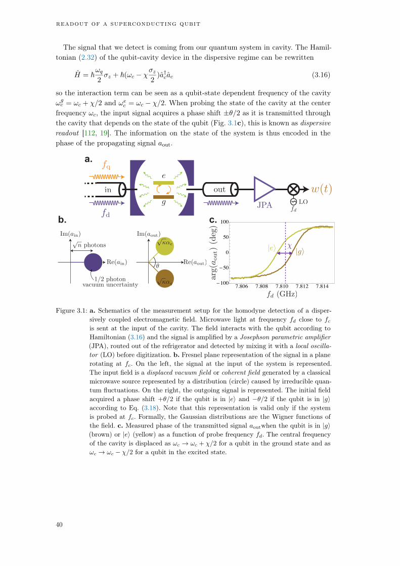
readout of a superconducting qubit
The signal that we detect is coming from our quantum system in cavity. The Hamil-tonian (2.32) of the qubit-cavity device in the dispersive regime can be rewritten
H = ~!q
2z + ~(!c
z
2)a†cac (3.16)
so the interaction term can be seen as a qubit-state dependent frequency of the cavity!gc = !c + /2 and !e
c = !c /2. When probing the state of the cavity at the centerfrequency !c, the input signal acquires a phase shift ±/2 as it is transmitted throughthe cavity that depends on the state of the qubit (Fig. 3.1c), this is known as dispersivereadout [112, 19]. The information on the state of the system is thus encoded in thephase of the propagating signal aout.
a.
b. c.
7.806 7.808 7.810 7.812 7.814100
50
0
50
100
Figure 3.1: a. Schematics of the measurement setup for the homodyne detection of a disper-
sively coupled electromagnetic field. Microwave light at frequency fd close to fcis sent at the input of the cavity. The field interacts with the qubit according to
Hamiltonian (3.16) and the signal is amplified by a Josephson parametric amplifier
(JPA), routed out of the refrigerator and detected by mixing it with a local oscilla-
tor (LO) before digitization. b. Fresnel plane representation of the signal in a plane
rotating at fc. On the left, the signal at the input of the system is represented.
The input field is a displaced vacuum field or coherent field generated by a classical
microwave source represented by a distribution (circle) caused by irreducible quan-
tum fluctuations. On the right, the outgoing signal is represented. The initial field
acquired a phase shift +/2 if the qubit is in |ei and /2 if the qubit is in |giaccording to Eq. (3.18). Note that this representation is valid only if the system
is probed at fc. Formally, the Gaussian distributions are the Wigner functions of
the field. c. Measured phase of the transmitted signal aoutwhen the qubit is in |gi(brown) or |ei (yellow) as a function of probe frequency fd. The central frequency
of the cavity is displaced as !c ! !c + /2 for a qubit in the ground state and as
!c ! !c /2 for a qubit in the excited state.
40

3.2 dispersive readout
More quantitatively, Gambetta et al. have shown in a seminal paper [113] that thefield inside the driven cavity evolves depending on the qubit state according to the firstorder equations
8
><
>:
d↵g(t)
dt= i(!d !c
2)↵g(t)
2↵g(t) + d
d↵e(t)
dt= i(!d !c +
2)↵e(t)
2↵e(t) + d
. (3.17)
Here is the decay rate of the cavity, is the cavity pull and d is the drive strength.The steady state values of the field are obtained by canceling the left side of (3.17)
↵g =2d
+ i 2i(!d !c)and ↵e =
2d i 2i(!d !c)
(3.18)
In transmission, the output field is related to the intra cavity field by haouti =pout hai where out is the damping rate of the cavity mode through the output port.
In our setup, the decay rate of the cavity is dominated by its coupling to the outputport so out ' . The two corresponding outgoing field amplitudes are represented onFig 3.1b when the cavity is in a steady state. By detecting Im(aout) we can reveal theinformation on the energy of the qubit and conversely the quadrature Re(aout) doesnot depend on the qubit state, an homodyne detection is thus well-suited. We use ahome made quantum-limited phase-preserving amplifier called Josephson parametricamplifier (JPA in Fig 3.1a) that amplifies the quadrature of interest at the expense ofthe other quadrature8 followed by commercial amplifiers that are not represented onthe figure for simplicity.
By using the measurement theory developed hereabove, the continuous time mea-surement record reads [44]
w(t)dt =pd h2Im(aout)i dt+ dWw(t) (3.19)
where d = 34% is the measurement efficiency of the detection setup. By assuming thatthe cavity field reached the steady state and that !d = !c, we can express
h2Im(aout)i =p h2Im(a)i = p
hzi↵e ↵g
i= 2 hzi
s
n2
2 + 2(3.20)
where n = 4|d|2
2+2 is the average number of photon stored in the cavity. The signal tonoise ratio (SNR) of the measurement record (3.19) during dt is defined as
SNR(dt) =
pd h2Im(aout)i dt
dWw(t)
2
= d|↵e ↵g|2 hzi2 dt (3.21)
since dWw(t)2 = dt. The measurement rate Γm can be defined as half the signal to
noise ratio per unit of time when hzi = ±1
Γm =SNR(t)
2t=d
2|↵e ↵g|
2 =2dn
2
2 + 2(3.22)
8 See chapter 5 for a complete description of this amplifier.
41

readout of a superconducting qubit
-20 -10 0 10 20
0
500
1000
1500
2000
2500a. b.
0.0 0.5 1.0 1.5 2.00
5
10
15
20
Figure 3.2: a. Histograms of 5 104 integrated measurement records ↵R T
0w(t)dt for various
numbers of photons n indicated by the colors. The photon numbers are reported
as dashed lines in b. The integration time is T = 1 µs and ↵ is a proportionality
constant in mV that depends on the detection setup. The qubit is initialized in
(|gi+ |ei)/p2 and we observe the progressive separation of two peaks corresponding
to the qubit in either |gi or |ei. Their width is given by the combined effect of zero-
point fluctuations and the noise added by the detection setup. If the two peaks do
not overlap, the spin state is projected and the measurement is strong. When the
two peaks overlap, the experimentalist cannot distinguish between |gi and |ei and
the measurement is weak. b. Number of bits of information gained on the qubit
state by unit of time as a function of the stationary number of photons stored
in the cavity. We observe a linear dependence of Γm in the number of photons n
in agreement with Eq. (3.22) up to 1.5 photons. Beyond this number, the JPA
placed after the cavity (see Fig. 3.1) becomes non-linear because the high photon
flux at the amplifier input ‘exhausts’ the pump.
The scale factor 2 is arbitrary in (3.22), this particular choice is motivated becauseas defined Γm/ln(2) is the number of bits of information gained from the measurementper unit of time [114] (see Fig. 3.2b).
The measurement record thus takes the form
w(t)dt =p
2Γm hZi dt+ dWw(t), (3.23)
which exactly corresponds to (6.29) with a jump operator Lw =p
Γd/2z with Γm =
dΓd. According to equation (3.22), the measurement rate can be varied by tuning theinput power of the readout field ain that changes the stationary number of photon n
in the cavity. In Fig 3.2 are represented histograms of the integrated output signalR T0 w(t)dt for an increasing stationary number of photons in the cavity. When the two
distributions in Fig. 3.1 and 3.2 are well-separated, we can resolve the qubit state in asingle-shot manner, that is in one realization of the experiment. In this case, we knowif the qubit is in |gi or |ei and the qubit state is projected because we extract morethan one bit of information during the measurement time T . The measurement is thensaid to be strong. By increasing Γm well above any other time scale of the system, weenter the quantum jump regime [115]. The measurement records are discontinuous intime because the qubit state ‘jumps’ between the two pointer state values |gi and |eiand any unitary departure from this point is suppressed by Zeno effect [116]. When thetwo distributions overlap, the qubit state is not projected onto |ei or |gi, we talk about
42

3.2 dispersive readout
weak measurement. However, the density matrix of the system is updated conditionedon the measurement outcome to take into account the non-projective ‘kick’ caused bythe measurement.
Finally, we mention that this measurement scheme is routinely used in circuit QEDto perform a quantum tomography of a qubit state. In Fig. 3.3, we prepare arbitrarypure states on the surface of the Bloch sphere by applying a pulse on the qubit where 2 [0, 2] is the rotation angle of the unitary transformation and is the phase of thepreparation pulse. We then perform a quantum tomography of each prepared state bymeasuring the qubit strongly after having mapped x, y or z onto z by a
2 pulse.The measurement outputs span a sphere proving that any state on the Bloch surfacecan be faithfully extracted with this technique. Here, the fidelity of the tomography isF = 98% for an integration time of 2 µs.
b.a.
Figure 3.3: Quantum tomography by dispersive measurement a. Pulse sequence used for the
measurement. We prepare the qubit with a pulse φ with = k/12 for k =
0, 1, ..., 11 and = n/9 for n = 0, 1, ...8 and then perform a quantum tomography
with a fast gate ;, π2
x
or π2
y
followed by a strong dispersive readout of the cavity.
b. The raw averaged measurement outputs given by the 3 rotations correspond
to the three Bloch coordinates and they span a Bloch sphere when displayed in 3
dimensions.
3.2.2 AC stark shift and measurement induced dephasing
A direct measurable consequence of the dispersive interaction Hamiltonian is that in-creasing the average population of the cavity shifts the measured frequency of the qubit,this is known as the AC Stark shift. When driving the cavity with a coherent field at fdclose to fc, the field produced in the cavity follows a Poisson statistics so the qubit fre-quency itself follows a Poisson statistics. The average density matrix of the qubit is theweighted mean of Bloch vectors rotating at different angular velocities fq,n = fq n~.This loss of purity is dubbed measurement induced dephasing9 because this effect can
9 This phenomenon originates from noise in the qubit frequency which matches the photon shot noise.
43

readout of a superconducting qubit
be seen as an unread measurement of the qubit state by the cavity field described by aquantum map of the form (3.12). In this section we give the expression of the frequencyshift of the qubit and dephasing associated to this decoherence mechanism as a functionof the drive parameters in the steady state regime.
In the case of unread measurements performed by the cavity, we can model the deco-herence by the interaction Hamiltonian (3.16) and then trace out the electromagneticfield stored in the cavity. The resulting qubit dynamics is of the Lindblad form as shownat the beginning of this chapter with renormalized qubit frequency !q ! !+!stark anda jump operator L' =
p
Γd/2z. The Stark-shift frequency and measurement induceddephasing rate read [113]
(
Γd(t) = Im[↵g(t)↵e(t)]
!stark(t) = Re[↵g(t)↵e(t)]
(3.24)
-5 0 5-40-200
20
40
-40 -20 0 20 40-200
20
40
60
80
100
-5 0 5
-200
20
40
60
80
100a. b.
c. d.
-40 -20 0 20 40
-40-200
20
40
Figure 3.4: a. and b. Measured induced dephasing and Stark-shift as a function of the detuning
between the probe and the cavity for various input powers. The dephasing rates are
obtained by Ramsey interferometry in the presence of an electromagnetic field that
creates an extra dephasing and a frequency shift. We normalize the measurement
rate and Stark-shift by the relative dimensionless power of the input drive |d|2 to
show the validity of Eq. (3.25) up to maxd = 40 MHz2. We superimpose a theoretical
curve in black given by Eq. (3.25) with independently measured parameters =
24.9 MHz and = 23.6 MHz. c. and d. Numerical simulations of the Stark-
shift and dephasing rate given by Eq. (3.25) for various / ratios ranging from
0.56 to 2.22 and = 2 3.6 MHz. Note also that the Stark shift can become
negative for some / ratios.
44

3.3 measurement of fluorescence
In the steady state regime, we can use Eq. (3.18) and we obtain the explicit expres-sions
8
>>><
>>>:
Γd = 82|d|2
(2 + 4(!d !c)2 2)2 + 422
!stark =4|d|
22 + 4(!d !c)
2 2
(2 + 4(!d !c)2 2)2 + 422
(3.25)
These frequencies are measured by performing a Ramsey interferometry experimentwith a populated cavity. We prepare the qubit in the (|gi+ |ei)/
p2 superposition with
a /2 detuned pulse, wait for a given amount of time and then readout the cavityjust after a fast /2 rotation. We observe an exponentially decaying oscillation witha decay rate Γd + Γ2 and the frequency allows a precise measurement of ! + !stark.We performed such a measurement for a range of drive frequencies and input powersgathered in Fig. 3.4. Another important remark is that we use these measurements tocalibrate the attenuation of the line and convert an input power at the input of thedilution refrigerator in dBm into a number of photons10 n = 2+2
22 Γd in the cavityas shown in Fig. 3.2. We can thus prepare a coherent field containing on average a‘fraction’ of a photon in the cavity with our system with a predictable frequency shiftand coherence time reduction for the qubit.
3.3 measurement of fluorescence
3.3.1 Heterodyne detection of the fluorescence of a qubit
We call heterodyne detection, the simultaneous measurement of the two quadraturesof an oscillating signal. It can be performed by down-conversion to a lower frequencyrange (compatible with the bandwidth of the digitization boards) using the mixingwith a tone produced by a local oscillator at a frequency close to the carrier frequencyof the signal. Similarly to the homodyne detection, the heterodyne detection is widelyused in signal processing and applications range from the celebrated superheterodyneradio receiver to current quantum optics experiments [111]. We propose here to collectthe fluorescence of a spin-1/2 by heterodyne detection [117, 23].
In our experiments, qubit pulses are generated by a microwave source modulated at afew tens of MHz (typically 50 MHz, orange drive in Fig. 3.5), the spontaneous emissionof the qubit is collected in the output port. The coupling rate of the input port of thecavity and the internal loss rate of the cavity are much smaller than the coupling rateto the output port of the cavity as depicted on Fig. 3.5. By doing so, we ensure thatthe large majority of the fluoresced field goes in the ouput port owing to Purcell effect.Indeed, coupling the cavity to a transmission line reduces the lifetime of the qubit (seechapter 2). It is also much more ‘likely’ that the qubit emits a photon in the outputport than into the input port because of the coupling rate asymmetry.
10 It is important to understand that an external drives populate the cavity in a coherent state of averagephoton number n and not a Fock state with a perfectly defined number of photons.
45
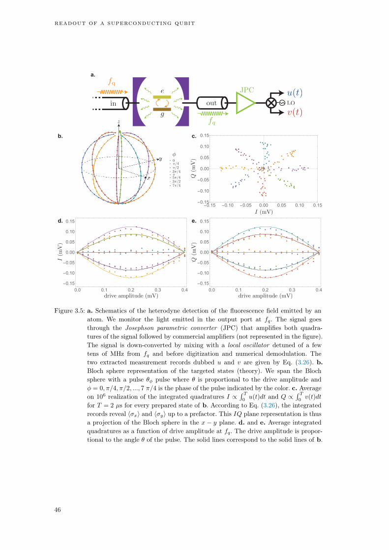
readout of a superconducting qubit
0.0 0.1 0.2 0.3 0.4
-0.15-0.10-0.050.00
0.05
0.10
0.15d. e.
0.0 0.1 0.2 0.3 0.4
-0.15-0.10-0.050.00
0.05
0.10
0.15
a.
-0.15 -0.10 -0.05 0.00 0.05 0.10 0.15-0.15-0.10-0.050.00
0.05
0.10
0.15b. c.
Figure 3.5: a. Schematics of the heterodyne detection of the fluorescence field emitted by an
atom. We monitor the light emitted in the output port at fq. The signal goes
through the Josephson parametric converter (JPC) that amplifies both quadra-
tures of the signal followed by commercial amplifiers (not represented in the figure).
The signal is down-converted by mixing with a local oscillator detuned of a few
tens of MHz from fq and before digitization and numerical demodulation. The
two extracted measurement records dubbed u and v are given by Eq. (3.26). b.
Bloch sphere representation of the targeted states (theory). We span the Bloch
sphere with a pulse φ pulse where is proportional to the drive amplitude and
= 0,/4,/2, ..., 7 /4 is the phase of the pulse indicated by the color. c. Average
on 106 realization of the integrated quadratures I /R T
0u(t)dt and Q /
R T
0v(t)dt
for T = 2 µs for every prepared state of b. According to Eq. (3.26), the integrated
records reveal hxi and hyi up to a prefactor. This IQ plane representation is thus
a projection of the Bloch sphere in the x y plane. d. and e. Average integrated
quadratures as a function of drive amplitude at fq. The drive amplitude is propor-
tional to the angle of the pulse. The solid lines correspond to the solid lines of b.
46

3.3 measurement of fluorescence
The signal is then amplified by a phase-preserving amplifier named Josephson para-metric converter (JPC)11. In this process the phase of the signal is preserved by am-plification and we detect both observables Re(aout) and Im(aout) associated with thetwo quadratures12 The amplified field is mixed with the signal of the same microwavesource that is used to generate the carrier of the input drive to avoid phase drifts. Theresulting signal is a low frequency field oscillating at 50 MHz that is digitized with anacquisition board and numerically demodulated to recover the I and Q quadratures.
In this case, the system is probed by the vacuum fluctuations of the electromagneticfields that can be viewed as triggering the emission of photons by the atom. So wecan apply the generalized measurement theory (6.29) with two jump operators Lu =pΓ#/2 and Lv = iLu corresponding to the two detected quadratures [85] where Γ#
is the de-excitation rate of the qubit and = (x iy)/2 is the lowering operator ofthe qubit. The measurement records read
8
><
>:
u(t)dt =q
fΓ#/2 hxi dt+ dWu(t)
v(t)dt =q
fΓ#/2 hyi dt+ dWv(t)(3.26)
where f = 14 % is the efficiency of the detection setup. Similarly to the homodynedetection, we can define a signal to noise ratio and the measurement rate of the fluo-rescence detection.
We show the integrated signalsRu(t)dt and
Rv(t)dt during T = 2 µs in Fig. 3.5 of
an undriven qubit relaxing after a preparation pulse for various and . As can beseen, this detection technique leads to the x and y Bloch coordinates of the qubit state.However the measurement rate associated to this tomography is set by the relaxationrate of the artificial atom Γ# = 50 100 kHz (variable from one run to the other). It isnot tunable in situ in contrast with the dispersive readout.
3.3.2 Destructive and QND measurements
In this section, we introduce the concepts of destructive measurement as opposed toquantum non-demolition measurement (QND). A QND measurement intuitively meansthat we are able to probe a quantum state without ‘destroying’ it [66]. For instance,when one photon is detected in a transmission line by heterodyne detection or byphotocounting the state of the wave packet carrying the photon is not projected, it isaltogether ‘demolished’. Instead of erasing the entire information on the state of thesystem, a QND measurement projects the state of the system in one of the pointerstates of the measurement and thus preserving information for subsequent quantumoperations. A second key ingredient of the definition is that two successive strongQND measurements should yield the same outcome. In the case of Von Neumannmeasurement a second measurement of the same observable immediately after the first
11 See chapter 5 for a detailed description of this amplifier.12 The two quadratures Re(a) and Im(a) of a quantum electromagnetic field do not commute. Pleasingly,
on top of amplifying the signal the JPC mixes the quadratures with an extra idler mode that transformsthe quadratures of the field in a set of commuting observables [26] at the price of adding an extra noiseto the signal corresponding to the zero-point fluctuations of this idler mode.
47

readout of a superconducting qubit
projection leads to the same outcome13. In the generalized measurement formalism, asufficient condition for QND measurement is that the interaction Hamiltonian betweenthe probe and the system commutes with the projector operator of the Von Neumannmeasurement performed on the probe [66]. But it is not necessary.
In the case of the dispersive interaction, information on the state of the qubit isimprinted in the phase of the electromagnetic field without destroying the state of thequbit. For large values14 of Γd, the measurement is repeatable and the state of thesystem is projected in |gi or |ei, which are the pointer states of the measurement. Thisprocess is thus QND even if the interaction Hamiltonian za†a does not commute withthe measured observable Im(a+ a†).
In the case of energy relaxation, one photon is emitted at the frequency of the qubitand we detect it by heterodyne detection. The interaction Hamiltonian and the mea-sured observables do not commute either. In this case the measurement erases theinformation on the quantum state by reseting the qubit in its ground state. In thestrong measurement limit i.e. Γ# much larger than any other inverse time scale, themeasurement has two possible outcomes corresponding to qubit having relaxed in itsground state after emitting one photon or no photons were emitted. The measurementcannot be repeated immediately after the emission of a photon without re-excitationof the qubit preventing this process to be a QND measurement. Lastly, we note thatwe monitor the expectation value of the operator which is not an observable15. Thefact that we are not ‘measuring’ an observable of the system can be understood by theopen nature of the system and in this case the quantum state of the system is convertedinto a propagating photon whose detection ‘destroys’ the state of the qubit.
3.4 full quantum tomography
In this section, we propose a novel detection setup combining the two previous ones.As we saw an heterodyne monitoring of the spontaneous emission of an atom divulgesinformation on its hxi and hyi components while an homodyne monitoring of the cav-ity in the dispersive regime reveals information on hzi. First, we show that performingthe two detections concurrently over a large number of realizations amounts to imagingthe Bloch vector. This technique is then used to monitor Rabi oscillations in the pres-ence of decoherence and our method is validated by comparison with the solution ofLindblad equation. Finally, we compare the fidelity of this quantum tomography withthe usual tomography protocol obtained from successive strong measurements of x,yand z components of the qubit.
3.4.1 Direct access to the Bloch vector
In the actual detection setup, we combine the two previous measurements16 (see Fig. 3.6).The spontaneous emission is at the frequency of the qubit fq ' 5.3 GHz while the
13 This not the case if we let the system evolve or relax between the two measurements.14 Much larger than any other time scale of the system.15 In particular, it is not Hermitian σ
† = σ+ = (σx + iσy)/2.
16 We can retrieve any of the previous situations by discarding the outputs of one of the detector.
48

3.4 full quantum tomography
dispersive readout is at the frequency of the cavity fc ' 7.8 GHz. The two signals arespatially separated by a commercial frequency diplexer TIGER TGF-A4214-001 placedin the output line17 (see Fig. 3.6). The signal is then routed out of the fridge via twodetection setups described in the previous sections namely two quantum limited am-plifiers are used to perfom an homodyne detection of the field at the frequency of thecavity and an heterodyne detection of the spontaneous emission at the frequency ofthe spin. The signal is then down-converted by mixing it with local oscillators beforedigitization and numerical demodulation.
2 cm
Figure 3.6: Schematics of the complete detection setup. We concurrently monitor the sponta-
neous emission of the atom at fq (green) and we probe the state of the cavity at
fd ' fc (purple). The two signals are spatially separated based on their frequencies
thanks to a commercial frequency diplexer. The complete measurement output is
a vector (u, v, w) given by Eq. (3.27) and its raw average scaled by the appropriate
prefactors is directly the Bloch vector (x, y, z). This method enables us to perform
a complete quantum tomography of the system without performing any gate on the
system.
We obtain simultaneously three measurement records
8
>>><
>>>:
u(t)dt =q
fΓ#/2 hxi dt+ dWu(t)
v(t)dt =q
fΓ#/2 hyi dt+ dWv(t)
w(t)dt =p
2dΓd hZi dt+ dWw(t)
. (3.27)
17 This is a key ingredient of our detection setup. It is in principle possible to replace the diplexer bya beam splitter but by doing so we would lose ‘half of the signal’ resulting in halving the detectionefficiencies.
49
readout of a superconducting qubit
A simple raw averaging provides a full quantum tomography of the system accordingto
0
BB@
x(t)
y(t)
z(t)
1
CCA
=
0
BB@
u(t)/pfΓ1/2
v(t)/pfΓ1/2
w(t)/p2dΓd
1
CCA
(3.28)
where . denotes the average over many realizations of the experiments. In order to ob-tain the Bloch vector, the two prefactors
pfΓ1/2 and
p2dΓd must be determined.
The rates Γ1 (15 µs)1 and Γd are respectively inferred from energy relaxation mea-surement and Ramsey oscillations in the presence of a populated cavity (see section3.2.2). The quantum efficiency f and d are obtained by SNR estimation or by reck-oning the back-action of the measurement18. In the actual experiments, the signal isintegrated during time steps dt = 100 ns and the records are amplified and filtered bythe detection chains19 so that we obtain (↵u,↵v,w) where ↵ and are the amplitudegains of the two chains. These scaling factors are precisely measured by looking at theamplitude of Rabi oscillations20. We can thus image the Bloch vector in time withoutperforming any quantum gates on the system in contrast with the usual tomographyprotocol of Fig. 3.3. This ‘gate free’ tomography is robust to any systematic errors onpulse calibration and relies instead on the estimation of the normalization constant ofthe chains.
In the following section, we confirm the validity of this readout technique in the caseof Rabi oscillation in the presence of decoherence by comparing the raw average of themeasurement records with the prediction of Lindblad equation.
3.4.2 Tomography of a qubit undergoing Rabi oscillations
In this experiment, the qubit is initialized in its thermal state close to the ground statewith an excitation probability of 2%. We apply a microwave drive on the device at thefrequency of the qubit, which acts as a driving torque of amplitude Ω around the Yaxis. We use the detection setup of Fig. 3.6 to observe the dynamics of the system inthe presence of weak decoherence (see Fig. 3.7).
The evolution of the state of the system is predicted by Lindblad equation
dtdt
= i[Ω
2y, t] +
Γd + Γ'
2D[z](t) + Γ#D[](t) + Γ"D[+](t) (3.29)
where Γ" = 1+zth2 Γ1 ' 0.75 ms is the thermal excitation rate of the qubit, D[L]() =
LL† 12(L
†L+L†L) is the Lindblad super-operator, zth = 0.96 is the z componentof the qubit at equilibrium and Γ# =
1zth2 Γ1 ' Γ1 = (15 µs)1 is the decay rate of the
qubit. The dephasing rates Γd = (5.0 µs)1 and Γ' = (17.9 µs)1 are respectively themeasurement induced dephasing rate and the pure dephasing rate. For an initial state
18 See chapter 6.19 In this chapter we make sure that dt is much smaller than any evolution and relaxation rate of the
system. We also take it greater than the inverse bandwidth of the amplifiers to avoid any time filteringof the signal by finite bandwidth of the JPA and JPC.
20 They can be equivalently inferred from noise correlations, see chapter 6 for details.
50

3.4 full quantum tomography
a. b.
Figure 3.7: Dynamics of a qubit undergoing a Rabi oscillation around the y axis from a thermal
state with 2% of excitation probability. The dots are the full quantum tomogra-
phy on the system obtained by raw averaging the measurement records given in
Eq. (3.28). The solid lines correspond to solutions of Eq. (3.29) with the parameters
Γ1 = (15 µs)1, Γφ = (17.9 µs)1, Γd = (5.0 µs)1 and Ω/2 = (2 µs)1 deter-
mined by independent projective measurements. a. Bloch sphere representation of
the evolution of the density matrix of the system. The color of the dots encodes the
evolution time 0 < t < 20 µs. b. Projections along the axes of the Bloch sphere as
a function of time, the color now encodes the axis of the projection. We observe a
good agreement between the continuous tomography and the solution of Lindblad
equation.
0 = 12(1 + x0x + z0z), the time evolution of the component of the Bloch vector is
confined in the x z plane and its components read8
<
:
x(t) = xinf + e(3Γ1+2Γϕ+2Γd)t4 [(x0 xinf)(cos(t) + sin(t)
Γ1 2Γϕ 2Γd
4+ (z0 zinf)
sin(t)Ω
]
z(t) = zinf + e(3Γ1+2Γϕ+2Γd)t4 [(z0 zinf)(cos(t) sin(t)
Γ1 2Γϕ 2Γd
4Ω) (x0 xinf)
sin(t)
Ω],
(3.30)
where rotation speed in the Bloch sphere around y is given by =
q
Ω2 (Γ12Γϕ2Γd)2
16
and the quantum state converges toward
xinf =2zthΩΓ1
Γ1(Γ1 + 2Γ' + 2Γd) + 2Ω2zinf =
zthΓ1(Γ1 + 2Γ' + 2Γd)
Γ1(Γ1 + 2Γ' + 2Γd) + 2Ω2(3.31)
in the long time limit.As depicted in Fig. 3.7, because of decoherence the state of the system experiences
under-damped oscillation toward the center of the Bloch sphere which is the maximallymixed state or most entropic state of the Bloch sphere. This damping is caused by thefact that we lose a part of our knowledge on the state of the system with time resultingin an increase of the entropy of the system. A good agreement between our tomographyand the solution of the Lindblad equation is found in Fig. 3.7 proving the validity of ourtomography. However it is interesting to compare the effectiveness of our tomographywith the usual tomography based on strong measurements.
51

readout of a superconducting qubit
3.4.3 Comparing the fidelities of a weak and projective quantum tomography
Our tomography protocol is a direct averaging of the measurement records (u, v, w)
on a large number of experiments N . Our tomography protocol highly differs fromthe usual technique that consists in measuring the three components of the qubit inseparate experiments by projective measurements and it is thus interesting to comparethe effectiveness of the two methods.
For the case of projective tomography, let us assume that we are able to measure anyaxis of the bloch sphere with a fast and single-shot readout of fidelity F = 1. After 3Nmeasurements, the probability distributions of the measurement records are given by abinomial distribution of +1 and 1 and the variance of the estimated Bloch coordinatesare Var(hxiestimated) =
1x2
N , Var(hyiestimated) =1y2
N and Var(hziestimated) =1z2
N .Three million experiments are thus needed to estimate an arbitrary state with a stan-dard deviation lower than 103. For our detection setup, the measurement recordsintegrated during a time dt are given by Eq. (3.27). In the limit of a large number N ofexperiments Var(hxiestimated) = Var(hyiestimated) =
2NfΓ1dt
and Var(hziestimated) =1
2NdΓddt. Thus, with the parameters of Fig. 3.7, 2 109 experiments are needed to
estimate an arbitrary state with a standard deviation lower than 103. For these pa-rameters, our method is much slower than the standard tomography to reconstructa density matrix at least for the small integration time dt = 100 ns chosen in ourexperiment.
Nevertheless, the average evolution of a quantum state evolving in time can only beaccessed by doing a set of quantum tomography at successive time steps. In Fig. 3.7,there are 198 time steps so reconstructing the evolution of the state of the qubit byprojective tomography would require 6108 experiments while 2109 experiments arestill required for tomography based on weak measurements. The signal to noise ratioof the tomography based on weak measurements is thus independent on the number ofsuccessive tomography and it becomes favorable in order to reconstruct lengthy evolu-tion of a qubit. More precisely, our method becomes more effective when reconstructingmore than 660 successive time steps. Alternatively, increasing the integration time dt
to higher values is straightforward with our setup21 and the variance of the outcomesis reduced as 1/dt. There is trade-off between the SNR of the measurement during asingle time-step and the number of time-step required to resolve the dynamics of thequbit.
Moreover, the convergence of the result of the projective tomography depends on thestate of the qubit and the variances of the signal vanish when the quantum state is ina pointer state of the measured observable. The reconstruction of the time evolution ofan oscillating qubit thus leads to a time varying uncertainty on the quantum state fora given number of realizations with the usual method. On the other hand, in the caseof weak tomography, the variance of the measurement records is independent of thestate of the system so our technique provides a uniform signal to noise ratio regardlessof the state of the system.
21 Note that the expression of the records (3.27) is only valid in the small dt regime. One has to integratethis expression to obtain the measurement outcomes integrated over time-scales that are not negligiblecompared to the characteristic time of evolution of the system.
52
3.5 conclusion
Finally, we assumed that the fidelity of the strong measurement is F = 1 but inpractice is it often limited by the fidelity of the readout process as well as the fidelity ofthe quantum gates. With our qubit parameters, even 100 ns long gates have a fidelitylower than 99 % because of the large dephasing on the qubit22. Our method does notrely on any quantum gates and therefore avoids this limitation.
3.5 conclusion
In this chapter we demonstrated
• a general theory for quantum measurement in continuous time limit with Krausoperators.
• the readout of a superconducting qubit by dispersive measurement both for weakmeasurement and tomography with the unavoidable decoherence associated tothe photon shot-noise of the cavity.
• the monitoring of the fluorescence field spontaneously emitted by an atom.
• a measurement scheme combining the monitoring of the two above mentioneddecoherence channels allowing for a continuous full quantum tomography of thequbit by direct raw averaging.
22 This rough estimation only takes into account Γϕ which is the fastest decoherence mechanism in ourexperiment.
53


4QUTRITS
4.1 introduction
As we saw in chapter 2 the transmon hosts about 10 levels inside the cosine potentialso the quantum physicist is not restricted to the first two levels of the artificial atomto store information and manipulate quantum states. This section is dedicated to thecoherent manipulation and readout of a three level system.
Morse code is based on a three letter alphabet: dashed, dot and space. This encodingwas widely used with the advent of the telegraph but modern communications use bi-nary signals. The quantum equivalent of Morse code is quantum communication withthree-state systems dubbed qutrits. A very good level of control was achieved withsuperconducting qutrits [118, 119] suggesting qutrits as a building block to achieveuniversal quantum computation [120]. Moreover, they are useful in communication pro-tocols such as quantum key distribution [121] and they are known to be more robust tocertain class of eavesdropping attacks [122]. Besides, they are routinely used in the su-perconducting circuits community to shape the temporal profile of single photons [123],to implement a quantum random generator [124] or to realize geometric phases [125].More broadly, multi level systems have many applications including the simplificationof quantum gates [126, 127, 119], the simulation and investigation of quantum chaos[128] or even for metrology [129].
4.2 preparation of an arbitrary quantum superposition of three
levels
If we go back to the BBQ formalism explained in section 2.2.1, we can write theHamiltonian of a transmon coupled to a cavity
H = ~!ca†cac + ~!ta
†t at EJ cos4('t(at + a†t) + 'c(ac + a†c)) (4.1)
where cos4(x) = cos(x) 1 + x2
2 , ac and ac (resp. at and a†) are the annihilationand creation operators of the cavity (resp. transmon). In the case of small zero pointfluctuation amplitudes 't,'c 1, we can restrict the cosine expansion to 4th order.In the dispersive regime, the Hamiltonian of a qutrit dispersively coupled to a cavityreads
H = ~!01 |1i h1|+ ~(!01 + !12) |2i h2| ~
3X
i=0
i |ii hi| a†cac (4.2)
where we denote by |0i, |1i, |2i1 the quantum states corresponding to a well definednumber of excitations in the transmon. The frequency of the g $ e qubit transition is
1 We equivalently use the notation |0i, |1i, |2i or |gi, |ei, |fi throughout this chapter.
55
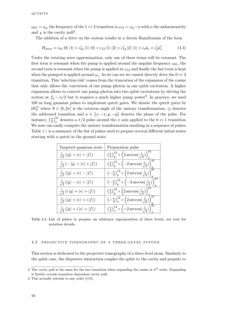
qutrits
!01 = !q, the frequency of the 1 $ 2 transition is !12 = !q↵ with ↵ the anharmonicityand is the cavity pull2.
The addition of a drive on the system results in a driven Hamiltonian of the form
Hdrive = 01 |0i h1|+ 01 |1i h0|+ 12 |1i h2|+ 12 |2i h1|+ dac + da†c. (4.3)
Under the rotating wave approximation, only one of these terms will be resonant. Thefirst term is resonant when the pump is applied around the angular frequency !01, thesecond term is resonant when the pump is applied at !12 and finally the last term is keptwhen the pumped is applied around !c. As we can see we cannot directly drive the 0 $ 2
transition. This ‘selection rule’ comes from the truncation of the expansion of the cosinethat only allows the conversion of one pump photon in one qubit excitation. A higherexpansion allows to convert one pump photon into two qubit excitations by driving thesystem at fq ↵/2 but it requires a much higher pump power3. In practice, we used100 ns long gaussian pulses to implement qutrit gates. We denote the qutrit gates by()ija where 2 [0, 2[ is the rotation angle of the unitary transformation, ij denotesthe addressed transition and a 2 x,x, y,y denotes the phase of the pulse. Forinstance,
2
01
xdenotes a /2 pulse around the x axis applied to the 0 $ 1 transition.
We now can easily compute the unitary transformation resulting in a sequence of pulses.Table 4.1 is a summary of the list of pulses used to prepare several different initial statesstarting with a qutrit in the ground state.
Targeted quantum state Preparation pulse1p3(|gi+ |ei+ |fi)
2
12
y
2 arccos( 1p3)01
y
1p3( |gi+ |ei+ |fi)
2
12
y
2 arccos( 1p3)01
y
1p3(|gi+ |ei |fi)
2
12
y
2 arccos( 1p3)01
y
1p3(|gi |ei+ |fi)
2
12
y
2 arccos( 1p3)01
y
1p3(i |gi+ |ei+ |fi)
2
12
y
2 arccos( 1p3)01
x
1p3(|gi+ |ei+ i |fi)
2
12
x
2 arccos( 1p3)01
y
1p3(|gi+ i |ei+ |fi)
2
12
x
2 arccos( 1p3)01
x
Table 4.1: List of pulses to prepare an arbitrary superposition of three levels, see text for
notation details.
4.3 projective tomography of a three-level system
This section is dedicated to the projective tomography of a three-level atom. Similarly tothe qubit case, the dispersive interaction couples the qubit to the cavity and permits to
2 The cavity pull is the same for the two transition when expanding the cosine at 4th order. Expandingit further reveals transition dependent cavity pull.
3 This actually extends to any order [105].
56

4.3 projective tomography of a three-level system
readout the energy state of the system. However it does not provide any information onthe relative phases of a superposition of states. It is in principle possible to reconstructthe full density matrix of a quantum system by placing a complete set of independentquantum operations ahead of a dispersive readout pulse.
4.3.1 From the measurement output to the density matrix
The density matrix of a qutrit is a 3 3 matrix positive and self-adjoint matrix
of trace one. The state of the system is thus fully determined by 9 independent realnumbers. Our tomography is achieved by 9 independent measurements with the set offollowing rotations prior to measurement
1,
2
01
x,
2
01
y,
2
12
x,
2
12
y,
2
12
x
2
01
x,
2
12
y
2
01
x. (4.4)
Other sets of pulses are possible [118] but we found this list to have the best fidelitywith our measurement setup and to be the least sensitive to pulse calibration errors4.The tomography protocols give a list of 9 complex outputs (s1, ..., s9). Each output sicorresponds to pulse i in (4.4). We can decompose
si = cg,i↵g + ce,i↵e + cf,i↵f (4.5)
with cg,i, ce,i, cf,i 0 and cg,i + ce,i + cf,i = 1. The complex amplitudes ↵g,↵e,↵f
represent the coherent state of the cavity in steady state regime when the qutrit isprepared in |gi , |ei , |fi. More quantitatively Gambetta et al. have shown [113] that inthe frame rotating at !c the stationary coherent field inside the cavity reads
8
>>>>>><
>>>>>>:
↵g =id
/2 i(!c !r )
↵e =id
/2 i(!c !r)
↵f =id
/2 i(!c !r + )
(4.6)
where d is the amplitude of the readout tone and !r its angular velocity. The complexamplitudes ↵i’s are represented in the quadrature plane in Fig. 4.1. Transmission signalsof the cavity are also shown for the parameters of the experiment.
Simple arithmetic manipulations show that the density matrix of the qutrit can beexpressed in terms of the measurement outputs
8
>>>><
>>>>:
11 = cg,1 22 = ce,1 33 = cf,1
12 = 21 = (ce,3 cg,3)/2 i(cg,2 ce,2)/2
13 = 31 = (ce,6 cf,6 + cf,4 ce,4)/p2 i(ce,7 cf,7 + cf,5 ce,5)/
p2
23 = 32 = (cf,5 ce,5)/2 i(ce,4 cf,4)/2
(4.7)
where we assumed that ii 2 R and ij = ji.
4 This is due to the symmetry of Eq. (4.7) that cancels out any systematic measurement error.
57
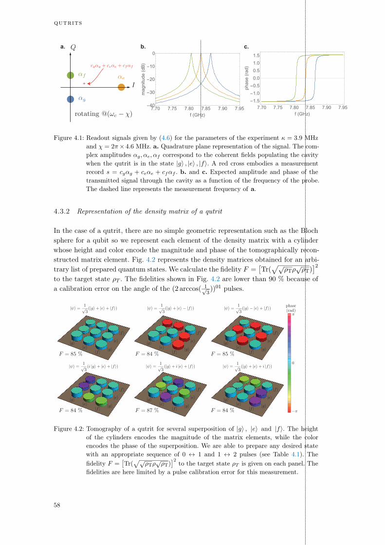
qutrits
+
7.70 7.75 7.80 7.85 7.90 7.95-40-30-20-100
f (GHz)
magnitude(dB)
7.70 7.75 7.80 7.85 7.90 7.95
-1.5-1.0-0.50.00.5
1.0
1.5
f (GHz)
phase(rad)
a. b. c.
Figure 4.1: Readout signals given by (4.6) for the parameters of the experiment = 3.9 MHz
and = 2 4.6 MHz. a. Quadrature plane representation of the signal. The com-
plex amplitudes ↵g,↵e,↵f correspond to the coherent fields populating the cavity
when the qutrit is in the state |gi , |ei , |fi. A red cross embodies a measurement
record s = cg↵g + ce↵e + cf↵f . b. and c. Expected amplitude and phase of the
transmitted signal through the cavity as a function of the frequency of the probe.
The dashed line represents the measurement frequency of a.
4.3.2 Representation of the density matrix of a qutrit
In the case of a qutrit, there are no simple geometric representation such as the Blochsphere for a qubit so we represent each element of the density matrix with a cylinderwhose height and color encode the magnitude and phase of the tomographically recon-structed matrix element. Fig. 4.2 represents the density matrices obtained for an arbi-trary list of prepared quantum states. We calculate the fidelity F =
Tr(pp
TpT)2
to the target state T . The fidelities shown in Fig. 4.2 are lower than 90 % because ofa calibration error on the angle of the (2 arccos( 1p
3))01 pulses.
Figure 4.2: Tomography of a qutrit for several superposition of |gi , |ei and |fi. The height
of the cylinders encodes the magnitude of the matrix elements, while the color
encodes the phase of the superposition. We are able to prepare any desired state
with an appropriate sequence of 0 $ 1 and 1 $ 2 pulses (see Table 4.1). The
fidelity F =Tr(pp
TpT)2
to the target state T is given on each panel. The
fidelities are here limited by a pulse calibration error for this measurement.
58

4.4 quadrature plane calibration and temperature measurement
The described projective tomography protocol can be used to track any operationon the qutrit. As an example we prepared a ‘GEF’ state | i = (|gi+ |ei+ |fi)/
p3 and
we let it relax to the ground state of the transmon. The evolution of the density matrixover time can be visualized in Fig. 4.3.
Figure 4.3: Tomography of the relaxation of a ‘GEF’ state. The qutrit is initialized in the
(|gi+ |ei+ |fi)/p3 state and a projective tomography is carried out every 250 ns
after the preparation.
4.4 quadrature plane calibration and temperature measurement
In this section, we show how to calibrate the I,Q quadrature plane of the readout signalof a qutrit. This calibration is instrumental to convert the measured signal in milliVoltsinto the coefficients cg, ce, cf in Eq. (4.5). We also give a simple protocol to estimatethe temperature of a 3D transmon qubit thanks to the control of the third level.
4.4.1 Calibration of the IQ plane
In this run, we had a ‘hot’ transmon with an effective temperature of the order of160 mK. The residual temperature of 3D transmons are commonly attributed to thecoupling to unknown hot bath (phonons of the substrate, quasi-particles, ...) that ran-domly injects excitations in the transmon mode. This effect could be caused by a poorthermalisation of the substrate or of the complete device or by an irradiation of highfrequency noise [130] routed by the microwave lines. Aluminum cavities usually havecolder transmons than copper cavities and we noticed that by etching the inner surfaceof the cavity before placing it inside the fridge, the residual temperature populationwas reduced. The proposed method for the temperature measurement is very simpleand efficient and it also gives an alternative way to measure gate fidelities for qubitand qutrit operations. At the end of the section, we compare this method with a ‘di-rect’ temperature measurement, which requires a single shot measurement with a goodsignal to noise ratio.
We cannot directly prepare a pure state |gi (resp. |ei or |fi) and measure the corre-sponding cavity transmissions because of the initial temperature of the qubit and the
59

qutrits
a. b.
-6 -5 -4 -3 -2 -1 0
-3-2-10
1
2
I (mV)
Q(mV)
***
*** 1
2345
Signal(mV)
0.0 0.1 0.2 0.3 0.4
1234
AmplDrive (V)
Signal(mV)
0.5
5
0
1
Signal(mV)
-101
2
Figure 4.4: a. Determination of ↵g, ↵e and ↵f . The 6 transmission amplitudes are indicated by
red stars. The solution of the system (4.9) gives the values of ↵g, ↵e and ↵f used
for the tomography. We superimpose in blue, green and orange measured Rabi
oscillations between the three levels of the qutrit along with linear interpolation
(solid lines). b. Rabi oscillations as a function of drive amplitude between different
levels projected along the lines drawn in a. The vertical axis origin matches the
dash on each line in a and the arrow indicates the sign of the signal. The dots are
the measured signal and the solid lines are sinusoidal fits. These Rabi oscillations
are used to calibrate our qutrit gates.
finite fidelities of the gates. We measure transmissions of the cavity having preparedthe qutrit in 6 different initial states with the following pulses
1, 01, 12 01, 12, 01 12, 01 12 01. (4.8)
The measurements are represented by red stars on Fig 4.4. We propose a simplifiedmodel to find the complex values of ↵g, ↵e and ↵f that relies on the following assump-tions
• We operate in a Hilbert space of dimension 3 namely pg + pe + pf = 1 where piis the probability to find the qutrit in state |ii after a measurement. There is noleakage to states |hi or higher.
• The qutrit is initially in a thermal state th corresponding to a Boltzmann distri-bution with a well-defined temperature T .
• We model the finite fidelity of the pulses of the transitions 0 $ 1 and 1 $2 by two numbers F and F 0. The density matrix ↵ |gi hg| + |ei he| becomes(F +(1F )↵) |gi hg|+(↵F +(1F )) |ei he| after a 01 pulse of fidelity F . Andsimilarly the density matrix ↵ |ei he|+ |fi hf | becomes (F 0+(1F 0)↵) |ei he|+(↵F 0+(1F 0)) |fi hf | after a 12 pulse of fidelity F 0. We thus assume that thereare no leakage to the |fi state during a 01 pulse and no leakage to the |gi stateduring a 12 pulse.
60

4.4 quadrature plane calibration and temperature measurement
We then solve the following system of coupled equations for the complex transmission(t1, ..., t6) corresponding to the pulses (4.8)
8
>>>>>>>>>>>>>>>>>>>>><
>>>>>>>>>>>>>>>>>>>>>:
t1 = pg↵g + pe↵e + pf↵f
t2 = (Fpe + (1 F )pg)↵g + (Fpg + (1 F )pe)↵e + pf↵f
t3 = (Fpe + (1 F )pg)↵g + (F 0pf + (1 F 0)(Fpg + (1 F )pe))↵e
+ (F 0(Fpg + (1 F )pe) + (1 F 0)pf )↵f
t4 = pg↵g + (F 0pf + (1 F 0)pe)↵e + (F 0pe + (1 F 0)pf )↵f
t5 = ((1 F )pg + F (F 0pf + (1 F 0)pe))↵g + (Fpg + (1 F )(F 0pf + (1 F 0)pe))↵e
+ (F 0pe + (1 F 0)pf )↵f
t6 = (F (F 0pf + (1 F 0)(Fpg + (1 F )pe)) + (1 F )(Fpe + (1 F )pg))↵g
+ (F (Fpe + (1 F )pg) + (1 F )(F 0pf + (1 F 0)(Fpg + (1 F )pe)))↵e
+ (F 0(Fpg + (1 F )pe) + (1 F 0)pf )↵f
(4.9)
where pg = 11+b+b2
, pe = b1+b+b2
and pf = b2
1+b+b2with the Boltzmann weight b =
e~!q/kBT . The resolution of (4.9) gives us the values of ↵g, ↵e, ↵f , the temperature T
and the fidelities F and F 0.From the measurements shown in Fig. 4.4, we extract the fidelities F = 95 % for
01 pusles and F 0 = 94 % for 12 pulses. We also obtain an 8 % probability to findthe qubit in the |ei state and 0.8 % probability to find the qubit in the |fi state,which corresponds to a qubit temperature of 160 mK. We thus demonstrated thatour model allowed us to infer the value of ↵g, ↵e and ↵f at rest. This calibrationis essential to obtain the density matrix of the qutrit by a projective tomography (seeprevious section). A similar temperature measurement method was used to measure theefficiency of a cooling protocol known as the double drive reset of population (DDROP)[86] in our group [85].
4.4.2 Direct temperature measurement
In this section, we show that etching the inner surface of the cavity reduces the residualtemperature of the transmon. We also use this opportunity to introduce a new temper-ature measurement based on a single-shot heterodyne measurement of the qubit in itsthermal state at the frequency fc /2 (see chapter 3). For this measurement the life-time of the qubit was increased to T1 = 15 µs and the cavity linewidth to ( 70 ns)1
by closing the output port of the cavity. We observe two separated probability distribu-tions corresponding to the qubit in state |gi or |ei. The probability to find the qubit inthe excited state is given by the relative weight of the two distributions, which has tobe measured in a time much longer than the inverse linewidth of the cavity and muchshorter than the lifetime of the qubit.
From Fig 4.5, we extract the probability to find the qubit in the excited state pe '1.8 % ± 0.2 % corresponding to an equilibrium with a bath at T ' 63 ± 2 mK. Wechecked that the two temperature measurement methods give compatible results duringthe same experimental run. Recently Serniak et al. [131] discovered that quasiparticles
61
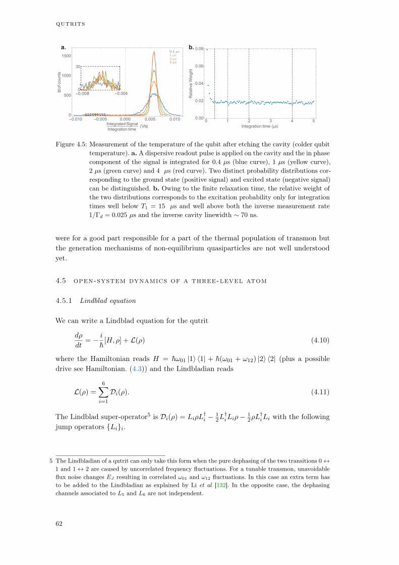
qutrits
-0.010 -0.005 0.000 0.005 0.0100
500
1000
1500
IntegratedSignal
Integration time(V/s)
#ofcounts
-0.008 -0.0040
30
a. b.
0 1 2 3 4 50.00
0.02
0.04
0.06
0.08
Integration time (μs)
Rela
tive
Weig
ht
Figure 4.5: Measurement of the temperature of the qubit after etching the cavity (colder qubit
temperature). a. A dispersive readout pulse is applied on the cavity and the in phase
component of the signal is integrated for 0.4 µs (blue curve), 1 µs (yellow curve),
2 µs (green curve) and 4 µs (red curve). Two distinct probability distributions cor-
responding to the ground state (positive signal) and excited state (negative signal)
can be distinguished. b. Owing to the finite relaxation time, the relative weight of
the two distributions corresponds to the excitation probability only for integration
times well below T1 = 15 µs and well above both the inverse measurement rate
1/Γd = 0.025 µs and the inverse cavity linewidth 70 ns.
were for a good part responsible for a part of the thermal population of transmon butthe generation mechanisms of non-equilibrium quasiparticles are not well understoodyet.
4.5 open-system dynamics of a three-level atom
4.5.1 Lindblad equation
We can write a Lindblad equation for the qutrit
d
dt= i
~[H, ] + L() (4.10)
where the Hamiltonian reads H = ~!01 |1i h1| + ~(!01 + !12) |2i h2| (plus a possibledrive see Hamiltonian. (4.3)) and the Lindbladian reads
L() =
6X
i=1
Di(). (4.11)
The Lindblad super-operator5 is Di() = LiL†i 1
2L†iLi 1
2L†iLi with the following
jump operators Lii.
5 The Lindbladian of a qutrit can only take this form when the pure dephasing of the two transitions 0 $
1 and 1 $ 2 are caused by uncorrelated frequency fluctuations. For a tunable transmon, unavoidableflux noise changes EJ resulting in correlated ω01 and ω12 fluctuations. In this case an extra term hasto be added to the Lindbladian as explained by Li et al [132]. In the opposite case, the dephasingchannels associated to L5 and L6 are not independent.
62

4.5 open-system dynamics of a three-level atom
Symbol Expression Physical meaning
L1
q
Γ01# |0i h1| spontaneous deexcitation 0 ! 1
L2
q
Γ01" |1i h0| spontaneous excitation 1 ! 0
L3
q
Γ12# |1i h2| spontaneous deexcitation 2 ! 1
L4
q
Γ12" |2i h1| spontaneous excitation 1 ! 2
L5
qΓ01φ
2 (|1i h1| |0i h0|) pure dephasing 0 $ 1
L6
qΓ12φ
2 (|2i h2| |1i h1|) pure dephasing 1 $ 2
Table 4.2: List of jump operators of a qutrit. Γij"(#) is the (de)excitation rate of the transition
ij and Γijφ is the random AC Stark shift rate of transition ij, which can be modeled
as fluctuations of !ij . We define the inverse lifetime of the i $ j transition as
Γij1 = Γ
ij# + Γ
ij" .
From the expression of the jump operators 4.2, we can write the Lindbladian explicitlyas follow
L() =1
2
0
BB@
2(Γ01#
ρ11Γ01"
ρ00) (Γ01#
+Γ01"
+Γ12"
+2Γ01φ
+Γ12φ
)ρ01 (Γ01"
+Γ12#
+Γ01φ
+Γ12φ
)ρ02
(Γ01#
+Γ01"
+Γ12"
+2Γ01φ
+Γ12φ
)ρ10 2(Γ01"
ρ00Γ01#
ρ11)+2(Γ12#
ρ22Γ12"
ρ11) (Γ01#
+Γ12#
+Γ12"
+2Γ12φ
+Γ01φ
)ρ12
(Γ01"
+Γ12#
+Γ01φ
+Γ12φ
)ρ20 (Γ01#
+Γ12#
+Γ12"
+2Γ12φ
+Γ01φ
)ρ21 2(Γ12"
ρ11Γ12#
ρ22)
1
CCA
(4.12)
In the following section we will measure the different rates in 4.2 and check that theEq. (4.10) indeed predicts the average evolution of the density matrix of the qutrit.Obviously the qubit case is recovered by setting all the relaxations rates Γi2 and drivesi2 to zero.
4.5.2 Energy relaxation
In this experiment, we first excite the qutrit with two successive drives at !01 and !12
(see Fig. 4.6) and we then monitor the evolution of the populations of the density matrixby tomographic reconstruction [118, 119]. The evolution of the populations reads
8
>>>>><
>>>>>:
d00dt
= Γ01# 11 Γ
01" 00
d11dt
= Γ01" 00 (Γ01
# + Γ12" )11 + Γ
12# 22
d22dt
= Γ12" 11 Γ
12# 22
(4.13)
This measurement allow us to extract the value of the matrix elements (Γ01# )1 =
(12 ± 0.5) µs and (Γ12# )1 = (6 ± 0.5) µs as well as an estimation of the heating rates
(Γ01" )1 80 µs and (Γ12
" )1 > 100 µs. The heating rates can only be estimatedasymptotically on time scales of the order of Γ1 hence the previous estimation for this30 µs long measurement (see previous sections for the temperature measurements witha good accuracy).
63

qutrits
0 5 10 15 20 25 30
0.0
0.2
0.4
0.6
time (μs)
Population
0.3 0.2 -0.1 0.0
-0.3-0.2-0.10.0
0.1
I (mV)
Q(mV)
c.
b.
a.
Figure 4.6: a. Pulse sequence. We successively excite the 0 $ 1 and 1 $ 2 transitions and
then measure the population of the density matrix of the qubit by dispersive mea-
surement. b. Raw signal in the IQ plane for 30 µs of relaxation. We observe a
relaxation from ↵f toward ↵g. The line is curved in the direction of ↵e because the
matrix element Γ02# is absent from (4.13). c. Extracted population as a function of
time. The solid lines are the solution of Eq. (4.13).
4.5.3 Ramsey experiments
Similarly to the previous experiment we can realize any kind of experiment involvinga unitary evolution and Lindbladian (4.12). By analogy with the qubit, we perfomRamsey experiments [118, 119] between the two transitions by imprinting a rotationon the coherences of the density matrix. We initialized the qubit in a superposition of|gi and |ei (Fig. 4.7 a) or |ei and |fi (Fig. 4.7 b) and let the coherences of the densitymatrix rotate in order to measure the coherence times of the qutrit.
The Ramsey like experiments in Fig. 4.7 enable us to determine the decoherencetimes characterizing the qubit as well as the precise values of !01 ans !12 within anaccuracy of few tens of kHz, which is below the typical fluctuation rate of transmonqubits. From Fig. 4.7, we extract the values of the coherence times of our qutrit T 01
2 =
(Γ01# +Γ
01" +Γ
12" +2Γ01
+Γ12 )1 = (10.0± 0.2) µs and T 12
2 = (Γ01# +Γ
12# +Γ
12" +2Γ12
+
Γ01 )1 = (6.05 ± 0.2) µs. Interestingly, we find that T 01
2 (resp. T 122 ) has about the
same value as T 011 (resp. T 12
1 ) indicating that a quantum superposition of |0i and |1i(resp. |1i and |2i) would decohere in twice this amount of time solely because of puredephasing likely originating from residual thermal excitation of the cavity mode [133].
64
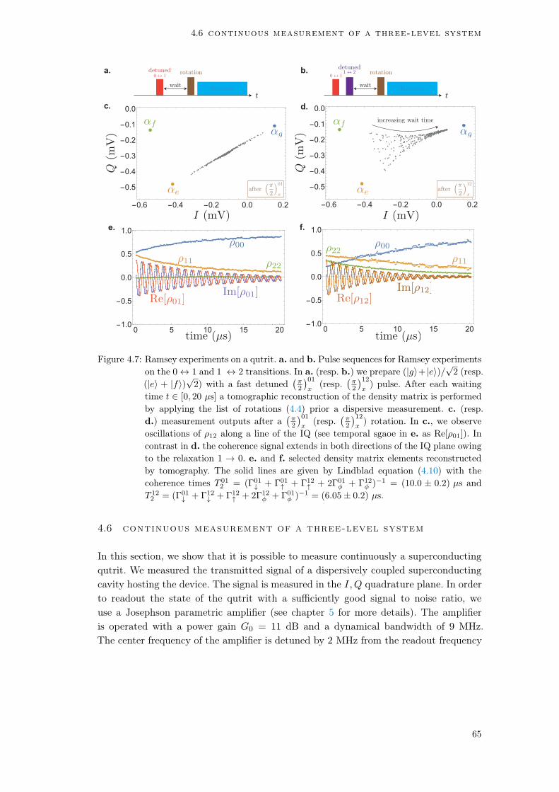
4.6 continuous measurement of a three-level system
0 5 10 15 20-1.0-0.50.0
0.5
1.0f.
0 5 10 15 20-1.0-0.50.0
0.5
1.0e.
-0.6 -0.4 -0.2 0.0 0.2
-0.5-0.4-0.3-0.2-0.10.0d.
-0.6 -0.4 -0.2 0.0 0.2
-0.5-0.4-0.3-0.2-0.10.0
c.
a. b.
Figure 4.7: Ramsey experiments on a qutrit. a. and b. Pulse sequences for Ramsey experiments
on the 0 $ 1 and 1 $ 2 transitions. In a. (resp. b.) we prepare (|gi+ |ei)/p2 (resp.
(|ei + |fi)p2) with a fast detuned
π2
01
x(resp.
π2
12
x) pulse. After each waiting
time t 2 [0, 20 µs] a tomographic reconstruction of the density matrix is performed
by applying the list of rotations (4.4) prior a dispersive measurement. c. (resp.
d.) measurement outputs after aπ2
01
x(resp.
π2
12
x) rotation. In c., we observe
oscillations of 12 along a line of the IQ (see temporal sgaoe in e. as Re[01]). In
contrast in d. the coherence signal extends in both directions of the IQ plane owing
to the relaxation 1 ! 0. e. and f. selected density matrix elements reconstructed
by tomography. The solid lines are given by Lindblad equation (4.10) with the
coherence times T 012 = (Γ01
# + Γ01" + Γ
12" + 2Γ01
φ + Γ12φ )1 = (10.0 ± 0.2) µs and
T 122 = (Γ01
# + Γ12# + Γ
12" + 2Γ12
φ + Γ01φ )1 = (6.05± 0.2) µs.
4.6 continuous measurement of a three-level system
In this section, we show that it is possible to measure continuously a superconductingqutrit. We measured the transmitted signal of a dispersively coupled superconductingcavity hosting the device. The signal is measured in the I,Q quadrature plane. In orderto readout the state of the qutrit with a sufficiently good signal to noise ratio, weuse a Josephson parametric amplifier (see chapter 5 for more details). The amplifieris operated with a power gain G0 = 11 dB and a dynamical bandwidth of 9 MHz.The center frequency of the amplifier is detuned by 2 MHz from the readout frequency
65
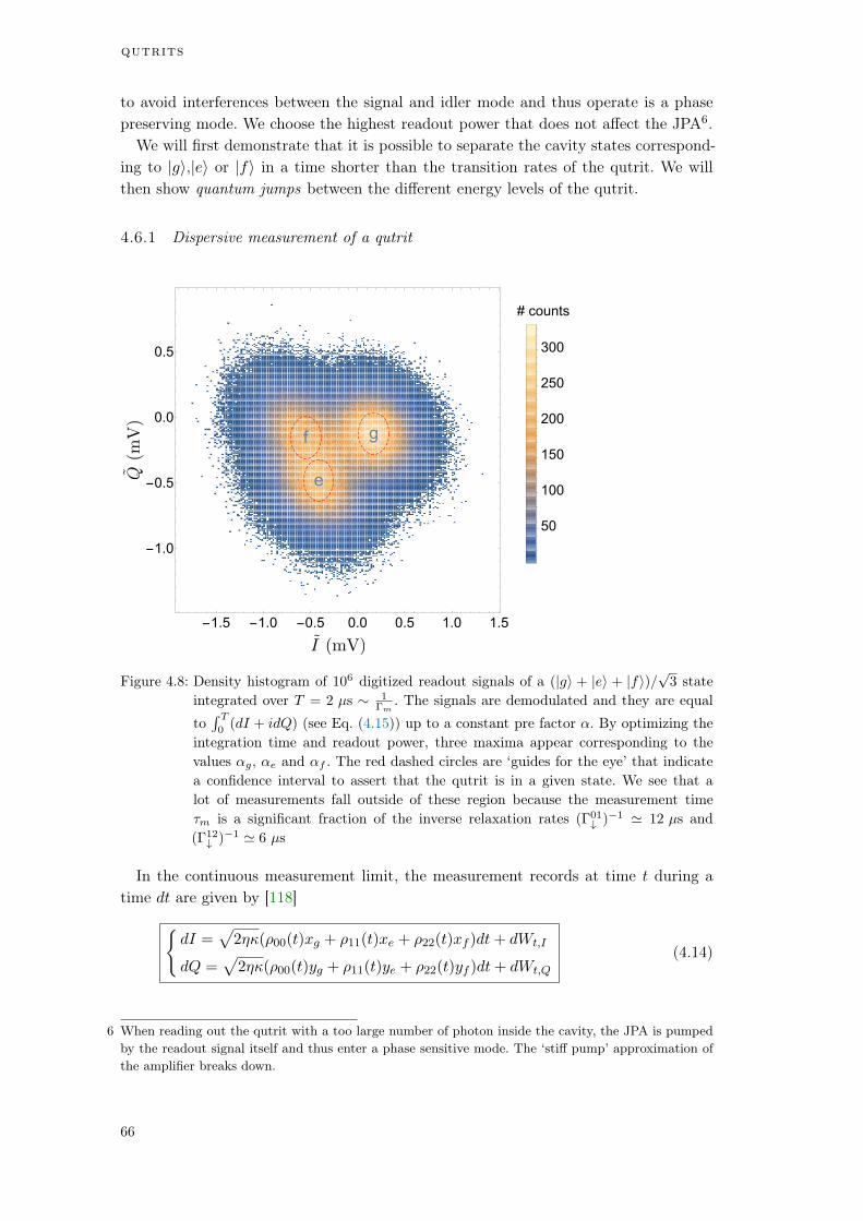
qutrits
to avoid interferences between the signal and idler mode and thus operate is a phasepreserving mode. We choose the highest readout power that does not affect the JPA6.
We will first demonstrate that it is possible to separate the cavity states correspond-ing to |gi,|ei or |fi in a time shorter than the transition rates of the qutrit. We willthen show quantum jumps between the different energy levels of the qutrit.
4.6.1 Dispersive measurement of a qutrit
g
e
f
-1.5 -1.0 -0.5 0.0 0.5 1.0 1.5
-1.0
-0.5
0.0
0.5
50
100
150
200
250
300
# counts
Figure 4.8: Density histogram of 106 digitized readout signals of a (|gi + |ei + |fi)/p3 state
integrated over T = 2 µs 1Γm
. The signals are demodulated and they are equal
toR T
0(dI + idQ) (see Eq. (4.15)) up to a constant pre factor ↵. By optimizing the
integration time and readout power, three maxima appear corresponding to the
values ↵g, ↵e and ↵f . The red dashed circles are ‘guides for the eye’ that indicate
a confidence interval to assert that the qutrit is in a given state. We see that a
lot of measurements fall outside of these region because the measurement time
m is a significant fraction of the inverse relaxation rates (Γ01# )1 ' 12 µs and
(Γ12# )1 ' 6 µs
In the continuous measurement limit, the measurement records at time t during atime dt are given by [118]
(
dI =p
2(00(t)xg + 11(t)xe + 22(t)xf )dt+ dWt,I
dQ =p
2(00(t)yg + 11(t)ye + 22(t)yf )dt+ dWt,Q
(4.14)
6 When reading out the qutrit with a too large number of photon inside the cavity, the JPA is pumpedby the readout signal itself and thus enter a phase sensitive mode. The ‘stiff pump’ approximation ofthe amplifier breaks down.
66
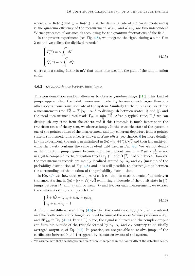
4.6 continuous measurement of a three-level system
where xi = Re(↵i) and yi = Im(↵i), is the damping rate of the cavity mode and
is the quantum efficiency of the measurement. dWt,I and dWt,Q are two independentWiener processes of variance dt accounting for the quantum fluctuations of the field.
In the present experiment (see Fig. 4.8), we integrate the signal during a time T =
2 µs and we collect the digitized records78
>>><
>>>:
I(T ) = ↵
Z T
0dI
Q(T ) = ↵
Z T
0dQ
(4.15)
where ↵ is a scaling factor in mV that takes into account the gain of the amplificationchain.
4.6.2 Quantum jumps between three levels
This non demolition readout allows us to observe quantum jumps [115]. This kind ofjumps appear when the total measurement rate Γm becomes much larger than anyother spontaneous transition rate of the system. Similarly to the qubit case, we definea measurement rate Γ
ijm =
2 |↵i ↵j |2 to distinguish between states |ii and |ji and
the total measurement rate reads Γm = minij
Γijm. After a typical time, Γ
1m we can
distinguish any state from the others and if this timescale is much faster than thetransition rates of the system, we observe jumps. In this case, the state of the system isone of the pointer states of the measurement and any coherent departure from a pointerstate is suppressed. This effect is known as Zeno effect (see chapter 6 for more details).In this experiment, the qutrit in initialized in (|gi+|ei+|fi)/
p3 and then left undriven,
while the cavity contains the same readout field used in Fig. 4.8. We are not deeplyin the ‘quantum jump regime’ because the measurement time T = 2 µs 1
Γmis not
negligible compared to the relaxation times (Γ01# )1 and (Γ12
# )1 of our device. However,the measurement records are mainly localized around ↵g, ↵e and ↵f (maxima of theprobability distribution of Fig. 4.8) and it is still possible to observe jumps betweenthe surroundings of the maxima of the probability distribution.
In Fig. 4.9, we show three examples of such continuous measurements of an undriventransmon starting in (|gi+ |ei+ |fi)/
p3 exhibiting a blockade of the qutrit state in |fi,
jumps between |fi and |ei and between |fi and |gi. For each measurement, we extractthe coefficients cg, ce and cf such that
(
I + iQ = cg↵g + ce↵e + cf↵f
cg + ce + cf = 1. (4.16)
An important difference with Eq. (4.5) is that the condition cg, ce, cf 0 is now relaxedand the coefficients are no longer bounded because of the noisy Wiener processes dWt,I
and dWt,Q in Eq. (4.14). In the IQ plane, the signal is blurred and the complex outputcan fluctuate outside of the triangle formed by ↵g, ↵e and ↵f contrary to an ideallyaveraged output si of Eq. (4.5). In practice, we are yet able to resolve jumps of thecoefficients between 0 and 1 triggered by relaxation events of the system.
7 We assume here that the integration time T is much larger than the bandwidth of the detection setup.
67
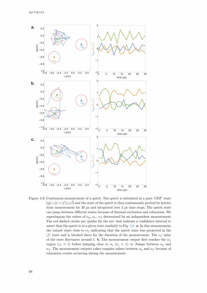
qutrits
-0.8 -0.6 -0.4 -0.2 0.0 0.2 0.41.0
-0.8-0.6-0.4-0.20.0
0.2
I (mV)
Q(mV)
-0.8 -0.6 -0.4 -0.2 0.0 0.2 0.4-1.0-0.8-0.6-0.4-0.20.0
0.2
I (mV)
Q(mV)
-0.8 -0.6 -0.4 -0.2 0.0 0.2 0.41.0
-0.8-0.6-0.4-0.20.0
0.2
I (mV)
Q(mV)
0 5 10 15 20 25 30-2-10
1
2
time (μs)
0 5 10 15 20 25 30-2-10
1
2
time (μs)
a.
b.
c.
0 5 10 15 20 25 30-2-10
1
2
time (μs)
Figure 4.9: Continuous measurement of a qutrit. The qutrit is initialized in a pure ‘GEF’ state
(|gi+|ei+|fi)/p3 and the state of the qutrit is then continuously probed by hetero-
dyne measurement for 30 µs and integrated over 2 µs time steps. The qutrit state
can jump between different states because of thermal excitation and relaxation. We
superimpose the values of ↵g, ↵e, ↵f determined by an independent measurement.
The red dashed circles are ‘guides for the eye’ that indicate a confidence interval to
assert that the qutrit is in a given state similarly to Fig. 4.8. a. In this measurement,
the output stays close to ↵f indicating that the qutrit state was projected in the
|fi state and is blocked there for the duration of the measurement. The cf value
of the state fluctuates around 1. b. The measurement output first reaches the ↵f
region (cf ' 1) before jumping close to ↵e (ce ' 1). c. Jumps between ↵g and
↵f . The measurement outputs takes complex values between ↵g and ↵f because of
relaxation events occurring during the measurement.
68

4.7 conclusion
This measure can be improved by increasing the gain of the quantum amplifier thatwould increase the detection efficiency of the measurement resulting in a stronger separa-tion of ↵g, ↵e and ↵f . The readout power could also be increased and the measurementtime decreased well below the characteristic times of the qutrit by increasing the pumppower of the JPA and thus enforce the stiff pump approximation for the amplifier. How-ever, it was not possible in our case to preserve a sufficient dynamical bandwidth tooperate the JPA as a phase-preserving amplifier.
4.7 conclusion
In this chapter, we demonstrated
• the coherent control of a three level system to prepare arbitrary superpositionsof three quantum states.
• the dispersive measurement of a qutrit in its energy basis.
• the observation of quantum jumps by continuous monitoring of the system.
• a good understanding of decoherence mechanisms of the qutrit.
• a method to estimate the thermal population of a qubit and the gate fidelities ofa qutrit.
These methods can readily be extended to populate and read out more than threelevels of the transmon. Note that the protection of the transmon against charge noiserequires larger and larger EJ/EC as the level number increases. With our transmonEJ/EC = 140 so all levels are addressable up to the 6th level as explained in the supple-mentary material of [105]. The projective tomography method requires 3 measurementsto reconstruct the density matrix of one qubit and 9 measurements for the density ma-trix of one qutrit. A 4 qutrits device has a Hilbert space of dimension N = 34 = 81
and (N 1) + 2N(N1)2 = 6560 real coefficients to determine so the use of higher di-
mensional Hilbert space requires an exponential number of measurements to achievethe full quantum tomography of the system.
We presented only linear readout methods with superconducting amplifiers but ageneralization to higher measurement power is an alternative way to obtain high fidelitysingle-shot measurements.
69


5MICROWAVE AMPL IF IERS
5.1 introduction
In the microwave domain, pumped circuits provide a complete toolbox to amplify sig-nals [134, 135, 136], engineer non classical states of light [137, 138], catch and releasequantum states [139], stabilize quantum states and manifolds [140, 88]. In this thesisI used three kinds of microwave amplifiers based on superconducting circuits namelythe Josephson Parametric Amplifier (JPA), the Josephson Parametric Converter (JPC)and the Josephson Traveling Wave Parametric Amplifier (JTWPA). The following sec-tions describe a general theory of quantum limited amplifiers and explain the operationprinciple of the above-mentioned amplifiers. Finally, we compare the figures of merit ofthe different amplifiers available in our laboratory.
The detailed fabrication processes of the JPA and JPC can be found in appendixB. The JTWPA was provided by the Lincoln Lab [136, 141] in 2017 and it was notused for the continuous time measurement presented in this thesis. At the end of thischapter, we compare the figure of merit of the different amplifiers namely gain, band-width, compression point, quantum efficiency and we explain the requirements for ourexperiments.
5.2 quantum parametric amplification
An amplifier can be modeled as a lumped device connected to two semi-infinite trans-mission lines that converts and amplifies an incoming quantum electromagnetic field aininto an outgoing field aout. Note that we restrict the discussion to scattering amplifiers.The elementary excitations of these fields are the carriers of the information that wewant to acquire. These electromagnetic modes are bosons so they verify the followingcommutation rule
[ain(t), a†in(t
0)] = [aout(t), a†out(t
0)] = (t t0) (5.1)
at all time t and t0. The nature of the amplifier is encoded in the scattering relation be-tween the incoming field and the re-emitted outgoing field. Naively one could think thatthe simplest amplifier would correspond to aout(t) =
pGain(t) but it is incompatible
with (5.1) so it is forbidden by quantum mechanics.
5.2.1 Phase preserving amplification
By introducing an additional operator bin called idler mode, one can write the relation
aout =pGain +
pG 1b†in. (5.2)
71
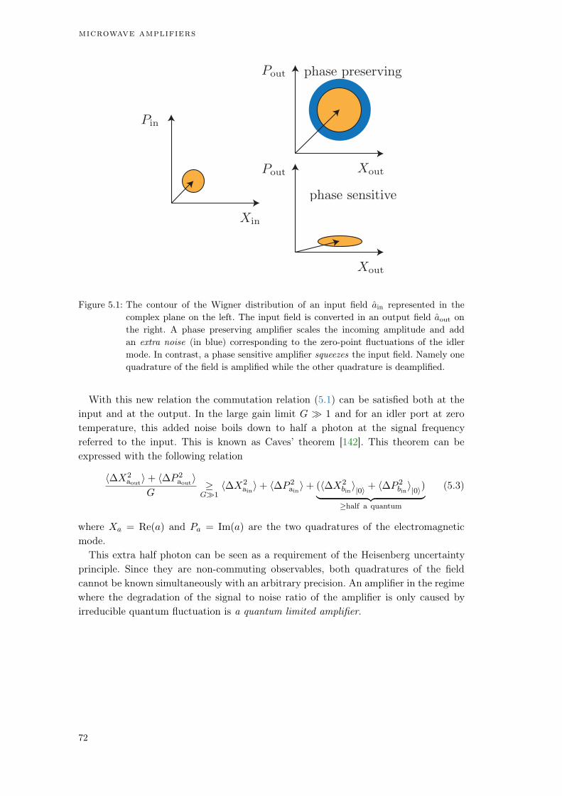
microwave amplifiers
Figure 5.1: The contour of the Wigner distribution of an input field ain represented in the
complex plane on the left. The input field is converted in an output field aout on
the right. A phase preserving amplifier scales the incoming amplitude and add
an extra noise (in blue) corresponding to the zero-point fluctuations of the idler
mode. In contrast, a phase sensitive amplifier squeezes the input field. Namely one
quadrature of the field is amplified while the other quadrature is deamplified.
With this new relation the commutation relation (5.1) can be satisfied both at theinput and at the output. In the large gain limit G 1 and for an idler port at zerotemperature, this added noise boils down to half a photon at the signal frequencyreferred to the input. This is known as Caves’ theorem [142]. This theorem can beexpressed with the following relation
h∆X2aouti+ h∆P 2
aoutiG
G1
h∆X2ain
i+ h∆P 2ain
i+ (h∆X2bini|0i + h∆P 2
bini|0i)
| z
half a quantum
(5.3)
where Xa = Re(a) and Pa = Im(a) are the two quadratures of the electromagneticmode.
This extra half photon can be seen as a requirement of the Heisenberg uncertaintyprinciple. Since they are non-commuting observables, both quadratures of the fieldcannot be known simultaneously with an arbitrary precision. An amplifier in the regimewhere the degradation of the signal to noise ratio of the amplifier is only caused byirreducible quantum fluctuation is a quantum limited amplifier.
72

5.3 josephson parametric amplifier
5.2.2 Phase sensitive amplification
Another way to satisfy the commutation relation (5.1) is to amplify one quadrature ofthe field while the corresponding conjugate quadrature is de-amplified
aout =pGain + ei
pG 1a†in (5.4)
for a given squeezing angle . We can see that in the large gain regime G 1 twoquadratures of the field are given by X
out = 2pGX
in and P out =
12pGP in. If the input
signal only consists in vacuum fluctuations, the amplifier squeezes the fluctuationsmaking the quadrature P less uncertain than the standard quantum limit (half aphoton) while the uncertainty on X is enhanced to preserve the Heisenberg uncertaintyprinciple.
5.3 josephson parametric amplifier
The Josephson Parametric Amplifier (JPA) is a single-mode parametric amplifier con-nected to one transmission line via a non reciprocal device called a circulator [143]. Ithas recently known a strong revival decades after the seminal work of Yurke et al. [32].This kind of device can be made out of a Josephson non linearity embedded into a /2microwave resonator.
a. b.
1 mm
10 μm
Figure 5.2: a. Circuit representation of the device. A SQUID composed of two Josephson junc-
tions is embedded into a /2 resonator coupled to the transmission line via a mi-
crowave circulator. b. Optical image of the device. We evaporated a /2 microstrip
aluminium resonator with a loop of two Josephson junctions forming a SQUID in
its center.
Under the Markov approximation and the rotating-wave approximation, the dynam-ics of the amplifier is governed by the Quantum Langevin Equation (QLE) equation
da
dt=
i
~[H, a]
2a+
pain(t) (5.5)
with H = ~!ra†a + ~K
2 (a†)2(a)2 the lowest order approximation of the Hamiltonian
where a and a† are the ladder operators of the oscillator with [a, a†] = 1, !r is the
73
microwave amplifiers
pulsation of the oscillator, K is the Kerr constant and is the coupling rate to thebath.
Note that,
• The Hamiltonian of the JPA can be found by considering a ‘BBQ’ version of theJPA [144]
H lumpedJPA = ~!0a
†a EJ
X
n>1
('2ZPF)
n
(2n)!(a+ a†)2n (5.6)
with the frequency of the lumped resonator !0 =p8EJEC/~ and 'ZPF =
2p
EC/~! are the reduced zero-point fluctuations of the flux. The transmon qubithas the same Hamiltonian but with a much higher non linearity. By expandingthe Hamiltonian to the first non-linear order, one obtains
H lumpedJPA ' ~!0a
†a EJ'4ZPF
24(a+ a†)4
'RWA
~!ra†a EJ
'4ZPF
4(a†)2(a)2.
(5.7)
This approximation is valid in the regime EC ~!r and the renormalized res-onator frequency is !r = !0EJ
'4ZPF2~ . Placing the junction in a resonator amounts
to replace 'ZPF by the total zero-point fluctuation of the flux but the non linearterm in the expansion (5.6) are of the same form.
• This oscillator is know in classical physics as the Duffing oscillator. It exhibits anabrupt transition when driven above a critical power. The operation principle ofthe Josephson Bifurcation Amplifier [100] relies on this sharp transition.
• The so-called Markov approximation assumes that the environment is ohmic.That means that the density of modes can be considered constant around thetransition frequencies of the circuit.
• The coupling constant to the bath is supposed to be small compared to anytransition frequency in (5.5).
It is possible to integrate the QLE and express the circuit variable a(t) as a functionof ain(t). The output field is obtained via the Input-Output relation
pa(t) = ain(t) + aout(t). (5.8)
Let us introduce the Fourier transformed operator a[!] =R +11 dtei!ta(t).
The QLE (5.5) now reads
i(! !r)
2
a[!] iKa†[!] a[!] a[!] +pain[!] = 0 (5.9)
We assume that the system receives a drive-tone at the input so intense that it canbe modeled by a coherent field of amplitude ↵in. The steady state of the intra-resonatorfield is then given by a coherent field ↵ such that
↵ =ip↵in
i2 + (! !r)K|↵|2
(5.10)
74

5.3 josephson parametric amplifier
7.90 7.92 7.94 7.96 7.98 8.00-3
-2
-1
0
1
2
3
f (GHz)
ph
ase
(ra
d)
X
7.75 7.80 7.85 7.90 7.95 8.00 8.05-60
-50
-40
-30
-20
f (GHz)
inp
ut
po
we
r(dBm
)
-3
-2
-1
0
1
2
3
phase
(rad)
a. b.
Figure 5.3: a. Phase of the reflected signal on an anharmonic oscillator as a function of in-
put power and frequency of the probe drive. A black cross marks the position
of the critical point of the oscillator. b. Horizontal cuts a for an input power
P = (50.5,45.5,40.5,32.5,33.5,33,32.5) dBm from darkblue to light-
blue (power is referred to the input of the dilution refrigerator). The dots are
the measured phases and the solid lines correspond to a fit with equation (5.10)
with !r = 2 7.966 GHz, = 43 MHz and the photon number calibration
K|↵|2 = (50.77(GHz))10P(dBm)/10. The theory developed in the text is consistent
for low powers but we see that the first non-linear order approximation in (5.7) is
not sufficient close to the critical point (lightblue).
The auto-consistent equation (5.10) exhibits a bifurcation at a critical input power|↵in|
2 = 1p27
K . When reaching this power, new solutions of equation (5.10) appear
leading to an instability of the system. The reflection response of a JPA device canbe seen in figure (5.3) where the critical point is marked with a black cross. Cuts ofthe 2D map are compared with the theory obtained by solving (5.10) and (5.8) with agood agreement below the critical point. For this device, internal losses were negligiblecompared to the coupling to the transmission line so all the information is containedin the phase of the outgoing signal.
5.3.1 Different JPAs and different pumping schemes
The denomination Josephson Parametric Amplifier encompasses a lot of different am-plifiers. A JPA can be a lumped non-linear element connected to a transmission line [32,36] or it can be embedded in a CPW or micro-strip resonator [33]. The non-linearitycan be distributed over several elements to increase the dynamical range of the device[37]. The resonator is usually coupled to the rest of the circuitry by a geometric capac-itance or impedance matched to the transmission line to enhance the gain bandwidthproduct of the amplifier [145]. Even for a given circuit design, several pumping schemesare available. The JPA can be pumped on resonance with a monochromatic micro-wavepump, with a bichromatic pump centered on its resonance frequency [35] or with a fluxmodulation at twice its frequency [34].
75

microwave amplifiers
c.
b.
a.
* * ** *
**
0 5 10 15 202
3
4
5
6
7d.
Figure 5.4: Frequency landscape for the differents pumping schemes of the JPA. The dashed
lines represent the response function of the device close to !r. a. First pumping
scheme: A monochromatic current pump (in red) is sent at the resonator frequency.
b. Second pumping scheme: A bichromatic current pump (in red) is centered around
the resonator frequency. c. Third pumping scheme: A monochromatic flux pump (in
orange) is applied at twice the resonator frequency. d. Degradation of the coherence
time of a 3D transmon followed by two isolators (40 dB of isolation) and a JPA
pumped with a monochromatic current pump (pumping scheme a). In this case
the frequency of the amplifier is matched with the frequency of the cavity of the
3D transmon. Increasing the pumping power will increase the amplifier gain but a
fraction of the pump tone unavoidably populates the cavity leading to a reduction
of the coherence time of the qubit by measurement induced dephasing.
Under different assumptions, all the three following pumping schemes lead to aneffective Hamiltonian of the form of a perfect one-mode squeezer
H = ~Ωa†a+~
2a†2 +
~
2a2 (5.11)
where Ω is the frequency of the amplifier in a rotating frame that depends on thepumping scheme and is the strength of the parametric pump. We are now going todetail the derivation of the Hamiltonian (5.11) for the three most common pumpingschemes.
a) Single pump
The first pumping scheme is the current-pumped JPA [33] where a monochromaticpump near resonance with the oscillator is used. Ap denotes the pump amplitude and!p its angular frequency. The pumped Hamiltonian is
H = ~!ra†a+
~K
2a†2a2 + ~Ap(e
i!pta† + ei!pta). (5.12)
In the displaced rotating frame of the pump a ! (a+ ↵)ei!pt, one obtains
H
~= (!r!p+2K|↵|2)a†a+
K
2(↵2a†2+↵2a2)+
K
2a†2a2+K(↵a†2a+↵a†a2) (5.13)
76
5.3 josephson parametric amplifier
under the condition i↵ = Ap+(ΩK|↵|2 i/2)↵ where Ω = !r!p+2K|↵|2, whichis exactly the QLE (5.9) for
pain = Ap. In the limit of small quantum fluctuations
'ZPF 1 and large pump |↵| 1 the two last terms in (5.13) are negligible and onefinds a squeezing Hamiltonian of the form (5.11) with a pumping amplitude = K↵2.
The squeezing Hamiltonian (5.11) is obtained in a displaced rotating frame andthere are tight constraints in order to fully neglect the cubic terms in (5.13). Anotherimportant drawback is that there are no spatial or spectral separation of the signal andthe pump tone. The pump tone can then leak into the rest of the circuit and causeunwanted effect on other devices matched at the same frequency. In figure (5.4d) isan example of the degradation of coherence time of a transmon due to the leakingof a pump tone of a well-isolated amplifier matched at the frequency of the cavityhosting the qubit. A way to circumvent this last difficulty is to cancel the pump toneby destructive interferences but the amplitude and phase of the cancelation tone hasto be recalibrated very often.
b) Bichromatic pump
A second way to obtain parametric amplification is by pumping the device with twosymmetric tones around its resonant frequency. The pump amplitudes are denoted Ai
and their angular frequencies are denoted !i. Similarly to (5.12), the Hamiltonian reads
H = ~!ra†a+
~K
2a†2a2 +
2X
i=1
Ai(ei!ita† + ei!ita). (5.14)
In a displaced rotating frame rotating at Ω12 = (!1+!2)/2 such that a ! aeiΩ12t+
↵1ei!1t + ↵2e
i!2t and under the condition ∆12 K|↵1||↵2|, one obtains
H
~'
RWA(!r+2K(|↵1|
2+ |↵2|2)Ω12)a
†a+K↵1↵2a†2+K↵
1↵2a
2+K
2a†2a2 (5.15)
under the assumption that ↵1 and ↵2 satisfy the coupled equations(
i↵1 = A1 + (!r !1 +K|↵1|2 i/2)↵1 +K(2|↵2|
2 + ↵1↵2e
i∆12t)↵1
i↵2 = A2 + (!r !2 +K|↵2|2 i/2)↵2 +K(2|↵1|
2 + ↵2↵1e
i∆12t)↵2
. (5.16)
In the limit of small quantum fluctuation, the squeezing Hamiltonian (5.11) is recov-ered with Ω = !r + 2K(|↵1|
2 + |↵2|2) Ω12 and = 2K↵1↵2 by neglecting the last
term in (5.15). We see that the cubic corrections in (5.15) are now safely neglected bythe application of the RWA. Moreover the spectral separation of the signal and pumptones allows an efficient filtering of the pump tones without the need of a cancellationscheme.
c) Flux pumping
A third way to obtain parametric amplification with a JPA is by directly modulatingthe inductance of a SQUID, which behaves as a flux-dependent non-linear inductance.This slight modification of the amplifier allows for flux pumping and DC flux biasing
77

microwave amplifiers
of the device in order to adjust its operating frequency as can be seen in figure (5.5 b).Let us start with the Hamiltonian (5.6). Replacing the junction by a SQUID modifiesthe Josephson energy such that
EJ ! EJ cos('ext) (5.17)
where 'ext = Φext2e~
is the reduced magnetic flux. We can decompose the magnetic fluxin (5.17) into the sum of a static component and an oscillatory component at angularvelocity !p 'ext = F + f cos(!pt), with f 1. We then separate the differentharmonics
EJ cos(F + f cos(!pt)) 'f1
EJ cos(F ) EJf sin(F ) cos(!pt)
EJf2 cos(F )
4cos(2!pt) + ...
(5.18)
Let us derive the Hamiltonian of the system at first order in f and fourth order in'ZPF with !p ' 2!0,
H ' ~!0a†a EJf sin(F ) cos(!pt)
'2ZPF
2(a+ a†)2
EJ'4ZPF
4!(a+ a†)4 (cos(F ) f sin(F ) cos(!pt)) + ...
'RWA
~!ra†a+ EJf
'2ZPF
2
a2ei!pt + a†2ei!pt
2 EJ
'4ZPF
4(a†)2(a)2
+ EJ'4ZPF
12(a†a3ei!pt + a†3aei!pt)
. (5.19)
In the limit of small quantum fluctuations, the two last '4 terms in (5.19) can bedropped. In the rotating frame a ! aei!pt/2 rotating at half the pump frequency, theHamiltonian is of the form of (5.11) with Ω = !r!p/2 and = EJf'
2ZPF/4~. A very
interesting point here is that the strength of the drive is in '2ZPF so it does not depend
on the Kerr non linearity of the resonator and in the small flux pump limit f 1, theleading correction are the same than for the bichromatic current pumped JPA. Also inthis last scheme, there is no displacement transformation to obtain (5.19).
d) Summary
Pumping scheme Frame a ! Ω
Single aeiωpt !r!p+2K|↵|2 K↵2
Bichromatic aeiΩ12t+↵1eiω1t+↵2eiω2t !r+2K(|↵1|2+|↵2|2)Ω12 2K↵1↵2
Flux a (lab frame) !rωp2
EJ δfϕ2ZPF
4~
Table 5.1: Comparison of the different pumping scheme of this section. In each case, we specify
the transformation used to obtain the squeezing Hamiltonian (5.11) with the corre-
sponding operating frequency of the amplifier in this frame as well as the strength
of the parametric pump.
In this thesis the second pumping scheme of table 5.1 was used to avoid the need ofa pump cancellation scheme and the addition on a on-chip flux pump.
78

5.3 josephson parametric amplifier
5.3.2 Amplification
All the previous pumping schemes are ways to obtain a squeezing Hamiltonian (5.11)
H = ~Ωa†a+~
2a†2 +
~
2a2 (5.20)
The equation of motion of the intracavity field is given by the QLE (5.5) in the framerotating at the frequency of the oscillator
/2 i! i
i /2 i!
!
a[!]
a†[!]
!
=p
ain[!]
a†in[!]
!
(5.21)
where ! = ! Ω, a[!] =R +11 dtei!ta(t) is the Fourier transformed signal mode and
a†[!] is the corresponding idler mode.By inverting the matrix in (5.21) and using the input-output relation (5.8), the
amplified signal reads
aout[!] = gS,!ain[!] + gI,!a†in[!] (5.22)
where the signal and idler amplitude gains are defined as8
>><
>>:
gS,! =(/2 i!)
(/2 i!)2 ||2 1
gI,! =i
(/2 i!)2 ||2
. (5.23)
The power gain is defined as G = |gS,!|2. In the large gain limit, we can approximate
||2 = 2
4 (1 + x) with x 1. The expression of the gain reads
G[!] =(2/2 + !2)2
(2/4)2x2 + 2!2 + !4. (5.24)
Close to the resonance frequency ! , the gain curve is a Lorentzian function andthe power gain reads
G[!] =G0
1 + (2!/)2(5.25)
where G0 = 4/ x2 is the power gain of the amplifier and the bandwidth of the resonance given by
= x/2 = /p
G0. (5.26)
We notice that with this first order theorypG0 is a constant. It is in fact a general
feature of any parametric amplifier that increasing the gain by increasing the pumppower comes with a reduction of the effective operating bandwidth1. An experimentallymeasured gain curve can be seen on Fig. 5.5. The power gain is G0 = 16 dB over abandwidth of 6.3 MHz leading to a gain-bandwidth product of
pG0 ' 39.8 MHz.
When the pump strength reaches a critical value |crit| =p
!2 + 2/4 the expressionof the amplitude gain gS,! diverges. The amplification of zero-point fluctuations leads to
79

microwave amplifiers
-0.5 0.0 0.57.4
7.6
7.8
8.0
8.2
8.4
a. b.
7.830 7.835 7.840 7.845
6
8
10
12
14
16
Figure 5.5: a. Power gain in reflection measured as a function of frequency. The dots correspond
to gains measured with a Vector Network Analyzer and the red solid line is a
Lorentzian function given by Eq. (5.25). We extract a gain G0 = 16 dB over a
bandwidth of 6.3 MHz from this fitting procedure. The gain-bandwidth product
ispG0 ' 39.8 MHz so the amplifier has a bandwidth of 4 MHz when operated
with a 20 dB power gain. b. Frequency of the resonator of the JPA as a function
of the external magnetic flux applied. The theory given by Eq. (5.30) (green line)
reproduces the experimental values (in blue) with a participation ratio p ' 2 %.
the generation of a large number of photons, this is known as parametric oscillation. Inpractice, the amplitude of the oscillation will be limited by additional extra non-linearterms that were not taken into account in the Hamiltonian (5.11).
An important point is that the Hamiltonian (5.11) corresponds to the case of a degen-erate amplifier for which only one electromagnetic mode is involved. If the measurementbandwith of the detection setup includes both the signal at ! and the idler mode at!, the device operates as a phase-sensitive amplifier [147]. On the contrary if theidler is filtered out, the amplifier is a phase preserving amplifier with power gain |gS,!|
2.This technique was used to implement an heterodyne readout of the state of a qutritin section 4.6.2.
It is also possible to use the same device as a non degenerate amplifier. For instance,pumping a /2-resonator JPA at a frequency close to 3!r/2 leas to amplification be-tween two distinct modes. The signal mode is the first cavity mode whereas the idleris the second harmonic of the resonator.
5.3.3 Frequency tunability
The typical bandwidth of such amplifiers is of the order of a few MHz when operated ata gain of 20 dB. An essential requirement for such a practical amplifier is to be frequencytunable in order to match other frequencies of the setup. In our implementation, thefrequency tunability is achieved by placing a SQUID in the middle of a /2 resonator.The inductance of the symmetric SQUID reads
LJ('ext) =LJ(0)
| cos('ext)|(5.27)
1 It is possible to avoid this constraint using reservoir engineering [146] or impedance matching [145].
80

5.4 josephson parametric converter
where LJ(0) is half of the inductance of a single junction in the SQUID. The JPA iscomposed of two /4 resonators of characteristic impedance Z0 linked by a SQUID. Bysymmetry, the electrical potential in the middle of the SQUID is 0 so the impedanceof the device ZJPA as seen from the transmission line is equal to the impedance ofa /4 resonator terminated by a load ZL = iLJ('ext)!/2 corresponding to half theimpedance of the SQUID [148]
ZJPA = Z0ZL + iZ0 tan(l)
Z0 + iZL tan(l)(5.28)
with = 2/ the angular wave number and l the effective length of the resonatorthat depends on the external flux. In the regime where the frequency of the resonatoris only slightly affected by the SQUID, one can write
!('ext) = !(0) + (!('ext) !(0))| z
!(0)
(5.29)
such that for a /4-resonator l ' 2 +
2!('ext)!(0)
!(0) and tan(l) ' 2!(0)(!('ext)!(0)) .
The resonance frequencies are the poles of the input impedance (5.28)
!r('ext) =!(0)
1 + p/| cos('ext)|, (5.30)
where p = !(0)LJ(0)/Z0 is the participation ratio of the SQUID to the inductanceof the resonator. The measured flux dependence is shown in Fig. 5.5b from which aparticipation ratio of 2% was inferred with a static bandwidth2 of the order of 600 MHz
justifying a posteriori the approximation of Eq. (5.29).
5.4 josephson parametric converter
The Josephson Parametric converter (JPC) was first built at Yale in 2010 [38] as a nondegenerate quantum limited microwave amplifier. The amplifier relies on a non linearelement known as the Josephson ring modulator (JRM) built with 4 Josephson junctionsin a Graetz bridge geometry which was later improved in our group in 2012 [39] byshunting the Josephson ring with linear inductances to increase its static bandwidth.
5.4.1 Josephson ring modulator
The Josephson ring modulator is analog of a Graetz bridge in which diodes are replacedby Josephson junctions. We will first describe the bridge and derive its Hamiltonianand then couple it to resonators to form a Josephson Parametric Converter. The ringis shunted by 4 linear inductances in order to increase the stability frequency range ofthe JRM and avoid phase-slip events. The Hamiltonian of the ring reads [40]
H = EJ(cos('a)+cos('b)+cos('c)+cos('d))+1
2EL('
2↵+'
2 +'
2 +'
2) (5.31)
2 Note that the dynamic bandwidth of the amplifier is the width of the gain curve in Fig. 5.5a whereasthe static bandwidth is the range of frequencies accessible in Fig. 5.5b by changing the operating pointof the amplifier.
81

microwave amplifiers
a. b.
Figure 5.6: Josephson ring modulator. a. Circuit diagram of the Josephson ring modulator
(JRM) consisting in a bridge of four identical junctions shunted by four linear
inductors. b. Optical microscope image of a Josephson ring modulator [40] analog
to the one used in the experiment. The Josephson junctions are marked by the blue
rectangles.
where EL ='20L is the magnetic energy associated to the shunt inductance and EJ
is the Josephson energy of the junctions. By assuming that the shunting inductancesparticipate symmetrically we can write
8
>>>><
>>>>:
'a = '2 '1 + 'ext/4 + 2na
'b = '3 '2 + 'ext/4 + 2nb
'c = '4 '3 + 'ext/4 + 2nc
'd = '1 '4 + 'ext/4 + 2nd
, (5.32)
where 'ext/4 is the reduced magnetic flux threading each sub-loop and (na, nb, nc, nd)
are the number of flux quanta threading the loops.It is then convenient to introduce the normal modes of the ring8
>>><
>>>:
'X = '3 '1
'Y = '4 '2
'Z =1
2('2 + '4 '1 '3)
. (5.33)
The Hamiltonian (5.31) can be rewritten in these new variables as
H = 4EJ cos('X/2) cos('Y /2) cos('Z) cos('ext/4)
4EJ sin('X/2) sin('Y /2) sin('Z) sin('ext/4)
+EL
4('2
X + '2Y + 2'2
Z)
(5.34)
82

5.4 josephson parametric converter
For small applied voltage at the nodes, we can expand the Hamiltonian (5.34) at 3rd
order in the normal modes
H = 4EJ cos('ext/4)
+1
2(EL
2+ EJ cos('ext/4))('
2X + '2
Y ) +1
2(EL + 4EJ cos('ext/4))'
2Z
EJ sin('ext/4)'X'Y 'Z .
(5.35)
The last term is the three wave mixing term that we wanted to generate with theJRM that is used for several application including quantum limited amplification ofmicrowave signals.
Note that a higher order expansion of (5.35) would reveal the following self-Kerr andcross-Kerr terms
H4thorder = EJ
6
'4X + '4
Y
16+ '4
Z
EJ
4
'2X'
2Z + '2
Y '2Z + '2
X'2Y /4
. (5.36)
Similarly to the JPA, the non linear element is inserted in microwave resonators thatare addressable via a 180 hybrid coupler (see Fig 5.8(a) for the actual implementation).The JRM is connected to two resonators that will define 3 spatially separated elec-tromagnetic modes that naturally couple to the modes X,Y and Z. The new modesof the whole circuit are denoted a, b and c and their quadratures are directly propor-tional to the quadratures of the normal modes X,Y and Z [40]. The three wave mixingHamiltonian of the device can be re-expressed as
H = ~!aa†a+ ~!bb
†b+ ~!cc†c+ ~(a+ a†)(b+ b†)(c+ c†). (5.37)
The modes a, b and c interact via higher order non linear terms (5.36), that lead tounwanted effects limiting the ideal behavior of the JPC as a linear amplifier as describedin the following section. It is the starting point of all the applications involving the JPC.
5.4.2 Amplification mode
The JPC is commonly used as an amplifier by applying a stiff classical pump p onthe common mode at a frequency !p = !a + !b, sum of the two non degenerate modefrequencies. The three wave mixing Hamiltonian then becomes
H
~= !aa
†a+ !bb†b+ (p+ p)(a+ a†)(b+ b†). (5.38)
By applying the rotating wave approximation on the Eq. (5.38) with the frequencymatching condition !p = !a + !b the rapidly oscillating term can be neglected so thatthe resulting Hamiltonian reads
H
~= !aa
†a+ !bb†b+ (pab+ pa†b†). (5.39)
The parametric down conversion term pa†b† can be understood as the annihilation ofone pump photon at !p and the creation of two photons at frequencies !a and !b. This
83

microwave amplifiers
8.1 8.2 8.3 8.4 8.5
0
10
20
30
7.9
8.1
8.3
8.5
8.7
-4π-8π 4π 8π0
a.
b.
Figure 5.7: Figure from [39]. a. Measured frequency of the resonator mode at !a as a function
of the external flux applied to the JPC without pump. b. Reflection gain on the
mode a as a function of frequency for various external fluxes encoded by the color
of lines in a.
a. b.
2 mm
Figure 5.8: a. Schematic of a practical implementation of the JPC. A 180 hybrid coupler is
used to excite the common mode with the pump tone and the mode a with the
signal. b. Optical image of a Josephson parametric converter in the microstrip ge-
ometry. The Josephson ring modulator is placed at the center of two /2 resonators
capacitively coupled to transmission lines.
84

5.4 josephson parametric converter
gives rise to the phenomenon of amplification in the JPC. Let us write the QLE formodes a and b
8
>><
>>:
@a
@t=
i
~[H, a] a
2a+
paain
@b
@t=
i
~[H, b] b
2b+
pbbin
, (5.40)
with a and b the coupling rates of modes a and b to the transmission lines. By takingEq. (5.40) to the Fourier domain and with the input-output relations
(paa[!] = ain[!] + aout[!]
pbb[!
0] = bin[!0] + bout[!
0], (5.41)
one obtains the scattering relation [135]
aout[!]
b†out[!0]
!
=
raa sab
sba rbb
!
ain[!]
b†in[!0]
!
(5.42)
where8
>>>>>>>>>>><
>>>>>>>>>>>:
raa =(1 b)(1 a) + ||2
(1 b)(1 + a) ||2
rbb =(1 + b)(1 + a) + ||2
(1 b)(1 + a) ||2
sab =2i
(1 b)(1 + a) ||2
sba =2i
(1 b)(1 + a) ||2
. (5.43)
with = 2p/pab, a = 2i(! !a)/a and b = 2i(!0 !b)/b. We defined the
cooperativity as C = ||2. The gain of the amplifier is defined by G = |raa|2 = |rbb|
2.In the large gain limit, the gain curve is given by a Lorentzian function close to
the frequency of the amplifier. For a detuning ∆! around the central frequency of theamplifier, the gain reads
G[∆!] =G0
1 + (2∆!/)2(5.44)
where G0 is the maximum gain and the bandwidth of the resonance reads
=2p
G0(1/a + 1/b). (5.45)
Measured gain curves are represented on Fig. 5.7(b). We achieved typical values ofG0 = 20 dB for the power gain over dynamical bandwidths of = 3 MHz.
When the pump is driven above the critical value C = 1, the parametric gain over-comes the damping rate of the electromagnetic modes and the oscillator enters theself-oscillation regime [149] similarly to the bifurcation physics of the JPA.
85
microwave amplifiers
5.4.3 Flux tunability
Similarly to the JPA, the operating frequency of the JPC can be tunned by applicationof an external magnetic flux because of the 'ext dependence of Eq. (5.35). This tunabil-ity enable the experimentalist to match the frequency of the system under study. Thefrequencies of modes a and b are adjustable by varying the external applied flux [39]
!a,b('ext) = !0a,b
2La,b/2
2La,b/2 + La,b('ext)(5.46)
where !0a,b is the bare frequency of the /2 resonator of mode a (resp. b) without the
JRM, La,b is its equivalent lumped inductance and La,b('ext) is the JRM inductance.As long as EL/4 + EJ cos('ext) > 0 the JRM inductance reads
La,b('ext) = '20
EL
2+ EJ cos('ext/4)
1
. (5.47)
The flux dependence of mode a can be observed in Fig. 5.7(a). The ‘stable configu-ration’ of the ring EL/4 + EJ cos('ext) > 0 corresponds to the wide arches. For smallshunting inductances 4 < EL/EJ , the stability condition is always met and the narrowarches disappear. The inductance of the ring is then always given by Eq. (5.47).
If we want to work on one of the wide arches and by noticing that a non zero fluxbias is required to obtain amplification3, we can estimate the overall flux tunability ofour amplifiers to be of the order of 300 MHz.
5.5 travelling wave parametric amplifier
The last amplifier that we use in our lab is the Josephson traveling wave parametricamplifier (JTWPA) [150, 151, 152, 136] provided by the Lincoln laboratory (MIT). Inthe section, we describe only briefly its principle of operation since the measurementsthat I performed with this amplifier are not reported in the present manuscript.
5.5.1 Phase matching condition
We saw from Eq. (5.26) and Eq. (5.45) that the gain bandwidth product of our amplifiersare limited by the linewidth of the resonant mode that hosts the non-linearity. In orderto get rid of this constraint, one can replace the stationary resonant mode stored in thecavity by a free propagating mode of a transmission line. However, the participationratio of the non linearity is diluted and the gain of the amplifier vanishes. A way tosolve this issue is to create a very long non linear transmission where the non linearityis distributed all over the line. The signal and a large pump tone are sent in thetransmission line and a four wave mixing process converts pairs of pump photons intoa signal photon and an idler photon. This four-wave mixing process has an hamiltonianof the form aPaPa
†Sa
†I and this process is resonant if and only if the pump and the signal
and idler mode are in phase all along the line. Obtaining this condition is challenging
3 Because of the sin(ϕext/4) dependence of the Hamiltonian (5.35).
86

5.5 travelling wave parametric amplifier
because the presence of a strong co-propagating pump modifies the phase velocitiesthrough self and cross Kerr effects hence generating a phase mismatch and preventingan exponential gain during the propagation. However, if this condition is satisfied, thenon linear transmission line implements the exact microwave analog of the celebratedoptic parametric amplifier [153].
The JTWPA is made of approximately two thousand of periodically repeated sectionscreating a lumped-element transmission line with a Josephson junction as the inductiveelement. In [136], every three unit cells of 16 µm, a lumped resonator is inserted inthe transmission line to ensure the phase-matching condition in agreement with theproposition of O’Brien et al. [152]. Several other attempts were carried out to fulfill thephase-matching condition such as periodic loading of TWPAs based on weak nonlinearkinetic inductance materials [150, 154] but they require a significantly higher pumppower to achieve comparable gains combined with a longer propagation length. Theyare also much more sensitive to backward parametric amplification because the phase-matching direction is satisfied for both directions.
In practice, building such an amplifier is very challenging because of the very largenumber of repeated sections and any impedance mismatch4 along the line or any in-homogeneity in the frequency of the resonators creates standing waves in the systemthat leads to ripples in the transmission signal as a function of frequency and thus afrequency-dependent gain (see Fig. 5.9 b and c).
5.5.2 Amplification performance
Getting rid of the gain-bandwidth constraint leads to remarkable performance as de-picted in the measurement of Greg Calusine in Fig. 5.9. We obtain a 20 dB gain overmore than 3 GHz in the 47 GHz frequency range (Fig. 5.9 c) corresponding to a gainbandwidth product beyond 30 GHz that outperforms our other quantum limited am-plifiers by more than two orders of magnitude. The JTWPA acts as a phase-preservingparametric amplifier because of the large spectral separation of the signal and idlermodes. By probing the unpumped device with a low power tone, the above-mentionedripples are observed as well as a large dip corresponding to a stop-band created by theresonators inserted along the line. The pump tone should be sent in the vicinity of thestop-band so that the phase-matching condition is met (red arrow on Fig. 5.9 b) andthe pump power is adjusted to obtain the desired gain at the frequency of interest. Thisstop-band in the dispersion relation prevents amplification on a 200 MHz window thatcan easily be avoided when designing our experiments. Finally, the amplifier operatesclose to the quantum limit as seen from the SNR improvement of the detection chain(Fig. 5.9 d) and total quantum efficiencies as high as 0.49% were reported in [136] forqubit readout experiments.
4 A special care must be taken to ensure a continuous impedance matching where the lumped filters areinserted by locally adjusting the parameters of the lumped element of the transmission line.
87
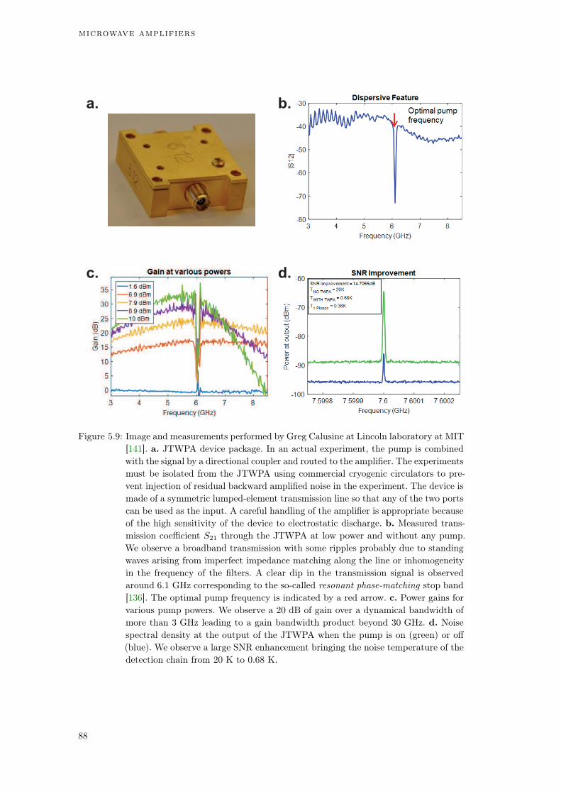
microwave amplifiers
a. b.
c. d.
Figure 5.9: Image and measurements performed by Greg Calusine at Lincoln laboratory at MIT
[141]. a. JTWPA device package. In an actual experiment, the pump is combined
with the signal by a directional coupler and routed to the amplifier. The experiments
must be isolated from the JTWPA using commercial cryogenic circulators to pre-
vent injection of residual backward amplified noise in the experiment. The device is
made of a symmetric lumped-element transmission line so that any of the two ports
can be used as the input. A careful handling of the amplifier is appropriate because
of the high sensitivity of the device to electrostatic discharge. b. Measured trans-
mission coefficient S21 through the JTWPA at low power and without any pump.
We observe a broadband transmission with some ripples probably due to standing
waves arising from imperfect impedance matching along the line or inhomogeneity
in the frequency of the filters. A clear dip in the transmission signal is observed
around 6.1 GHz corresponding to the so-called resonant phase-matching stop band
[136]. The optimal pump frequency is indicated by a red arrow. c. Power gains for
various pump powers. We observe a 20 dB of gain over a dynamical bandwidth of
more than 3 GHz leading to a gain bandwidth product beyond 30 GHz. d. Noise
spectral density at the output of the JTWPA when the pump is on (green) or off
(blue). We observe a large SNR enhancement bringing the noise temperature of the
detection chain from 20 K to 0.68 K.
88

5.6 figures of merit of amplifiers
5.6 figures of merit of amplifiers
In the above sections, we described the amplifiers available in our lab. We saw thatphase preserving amplifiers are suitable for heterodyne measurement of a quantumsignal whereas phase sensitive amplification is the best choice to perform an homodynemeasurement. Several other criteria are important to select the best practical amplifiersfor one given experiment. In this section, we enlighten the relevant figures of merit ofthe amplifiers presented in this chapter and we explain our amplification constraints tocarry out the quantum trajectories experiments described in section 6.2.
5.6.1 Amplifying setup
Our detection setup is composed of a succession of low noise amplifiers amplifiers asdepicted in Fig. 5.10 a that are designed to amplify low level signals with minimaladditive noise. However, the noise is amplified with the same gain as the signal inaddition to any additive noise. Therefore the amplifier cannot increase the signal tonoise ratio (SNR) as the signal level and the noise level rise with the same gain. Inthe case of narrow band amplifiers, the amplifier is able to filter signals that are out ofband but it cannot improve the SNR due to the in-band noise.
a.
b.
Figure 5.10: a. Typical input and output signal of a low noise amplifier. The signal and the
noise floor are amplified by the same gain leading to a similar SNR at the input
and at the ouput. The degradation of the SNR is due to additive noise referred to
the input of the amplifier. b. Amplifying chain composed of N low noise amplifiers
in series that take a low level signal at the input to a detectable voltage at the
end of the chain. Each amplifier has a gain Gi and a noise level Ni. In the large
G1 gain limit, the noise figure of the first amplifier dominates the noise figure of
the entire amplifying chain.
89
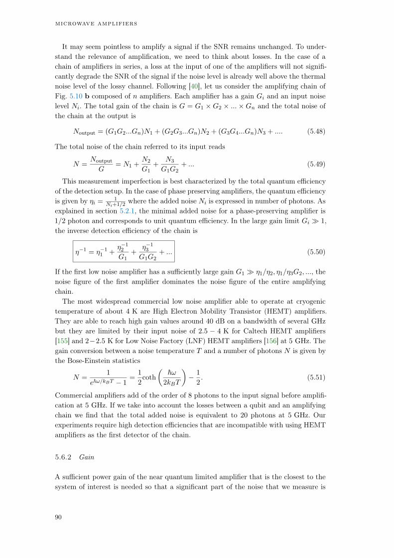
microwave amplifiers
It may seem pointless to amplify a signal if the SNR remains unchanged. To under-stand the relevance of amplification, we need to think about losses. In the case of achain of amplifiers in series, a loss at the input of one of the amplifiers will not signifi-cantly degrade the SNR of the signal if the noise level is already well above the thermalnoise level of the lossy channel. Following [40], let us consider the amplifying chain ofFig. 5.10 b composed of n amplifiers. Each amplifier has a gain Gi and an input noiselevel Ni. The total gain of the chain is G = G1 G2 ... Gn and the total noise ofthe chain at the output is
Noutput = (G1G2...Gn)N1 + (G2G3...Gn)N2 + (G3G4...Gn)N3 + .... (5.48)
The total noise of the chain referred to its input reads
N =Noutput
G= N1 +
N2
G1+
N3
G1G2+ ... (5.49)
This measurement imperfection is best characterized by the total quantum efficiencyof the detection setup. In the case of phase preserving amplifiers, the quantum efficiencyis given by i = 1
Ni+1/2 where the added noise Ni is expressed in number of photons. Asexplained in section 5.2.1, the minimal added noise for a phase-preserving amplifier is1/2 photon and corresponds to unit quantum efficiency. In the large gain limit Gi 1,the inverse detection efficiency of the chain is
1 = 11 +
12
G1+
13
G1G2+ ... (5.50)
If the first low noise amplifier has a sufficiently large gain G1 1/2, 1/3G2, ..., thenoise figure of the first amplifier dominates the noise figure of the entire amplifyingchain.
The most widespread commercial low noise amplifier able to operate at cryogenictemperature of about 4 K are High Electron Mobility Transistor (HEMT) amplifiers.They are able to reach high gain values around 40 dB on a bandwidth of several GHz
but they are limited by their input noise of 2.5 4 K for Caltech HEMT amplifiers[155] and 22.5 K for Low Noise Factory (LNF) HEMT amplifiers [156] at 5 GHz. Thegain conversion between a noise temperature T and a number of photons N is given bythe Bose-Einstein statistics
N =1
e~!/kBT 1=
1
2coth
~!
2kBT
1
2. (5.51)
Commercial amplifiers add of the order of 8 photons to the input signal before amplifi-cation at 5 GHz. If we take into account the losses between a qubit and an amplifyingchain we find that the total added noise is equivalent to 20 photons at 5 GHz. Ourexperiments require high detection efficiencies that are incompatible with using HEMTamplifiers as the first detector of the chain.
5.6.2 Gain
A sufficient power gain of the near quantum limited amplifier that is the closest to thesystem of interest is needed so that a significant part of the noise that we measure is
90

5.6 figures of merit of amplifiers
due to zero-point fluctuations. Operating a quantum limited amplifier with a 20 dB
power gain as the first amplifier of the chain followed by a HEMT brings the noisetemperature of the HEMT to about 0.08 photons at 5 GHz referred to the input of thechain. Roughly speaking, it means that about 16% of the measured noise is technicalnoise coming from the HEMT amplifier and the other 84% comes from zero-pointfluctuations5. In section 6.2, we measure quantum trajectories with a JPA operatedwith a gain of 22 dB and a JPC with a gain of 17 dB to make sure that the efficiencyof the detection chain is mainly limited by the efficiency of the first quantum limitedamplifier and not by the noise temperature of the following HEMT. A gain of 22 dB setan upper bound of 94% on the quantum efficiency of detection of the dispersive signalat 7.8 GHz while a gain of 17 dB set an upper bound of 70% on the quantum efficiencyof detection of fluorescence at 5.3 GHz.
5.6.3 Quantum efficiencies
The signal-to-noise ratio (SNR) of the measurement is limited by unavoidable lossesin the cables, insertion losses at the input of the amplifier in addition to the above-mentioned noise temperature of the HEMT. The losses in the lines and microwavecomponents (diplexer and circulators) before the signal reaches the amplifier are esti-mated to be at least of the order of 1.5 dB which leads to an efficiency cables 0.7.Since the first amplifier is not perfectly quantum limited, the inefficiency of the quan-tum amplifier itself is routinely modeled as a beam splitter with a transmission amplifier
followed by a lossless device. The beam splitter mixes the input signal with an extrachannel, which unavoidably comes with an additional noise. Intrinsic quantum efficien-cies of JPA and JPC can reach 1 in principle but they are often reported to have afinite value greater than 80% [40]. For the fluorescence signal we must introduce anadditional collection efficiency coll =
outtot
' 87% that contains the probability that aqubit emits a photon into the output line during a relaxation event [157]. In practiceour total quantum efficiencies are the product of all the above mentioned efficienciesand they were limited to 34% for the JPA and 14% for the JPC6.
5.6.4 Dynamical bandwidth
In order to measure the real time dynamics of a quantum system continuously, thedynamical bandwidth of the amplifier has to be larger than the typical rates and fre-quency of the evolution of interest. However, amplitude gain of the amplifier is inverselyproportional to the bandwidth of the amplifier (see Eq. (5.26)). The gain-bandwidthproduct of the device being constant, there is a tradeoff between reactivity and gain forour amplifiers. In practice we decided to operate both amplifiers with a bandwidth of4.25 MHz that led to the above-mentioned gains to reach a sampling time of dt = 100 ns
separating two successive independent measurements.
5 We assume in this simplified calculation that there is no extra added noise by the first amplifier of thechain.
6 We also showed by numerical simulation in section 6.4 that the quantum efficiency of the detectionsetup only qualitatively changes the statistics of quantum trajectories for efficiencies up to 75%.
91
microwave amplifiers
5.6.5 Static bandwidth
The frequency tunability of the amplifiers allows to shift the operating frequency ona range called the static bandwidth. It was of the order of 300 MHz for the JPC and500 MHz for the JPA. This figure characterizes our ability to match the center frequencyof each amplifier with either the frequency of the qubit or cavity. In practice it took usseveral tries to get the correct frequency agreement with decent quantum efficienciesbecause of fabrication uncertainties and aging of the junctions that shift the frequenciesfrom one cool-down to another.
5.6.6 Dynamical range
The 1 dB-compression point is defined by the amount of input power beyond whichthe power gain is reduced by 1 dB. The theories described above rely on the first orderexpansion of the cosine of the inductive part of the Hamiltonian. When the number ofphotons inside the amplifier increases this approximation breaks down and the powergain starts to deteriorate7. Higher order non linearities are known to limit not onlythe gain of the amplifiers but the quantum efficiencies and to introduce non gaussiansignatures in the output field [144]. 1 dB-compression points of the order of 120 dBm
are routinely reported for JPAs and JPCs. In our experiments, we operated withinthe single photon limit so the compression of the amplifier gain is negligible for bothmeasurements and this figure of merit is not important.
5.6.7 Comparison between two detection chains and a JTWPA
In the final year of this thesis, we received a JTWPA from Lincoln Labs [141], whichhas incredible performances in term of gain-bandwidth product and a very high 1 dB-compression point8 of 95 dBm when operated with a gain greater than 15 dB. Thisamplifier could have been used as a quantum limited amplifiers for both measurementchannels and total quantum efficiencies has high as 49% are reported for qubit readout[136]. However, using a phase preserving amplifier to perform an homodyne detectionleads to an effective reduction of the quantum efficiency of the chain. In current stateof the art experiments, the JTWPA is placed after JPAs or JPCs pre-amplifiers andimmediately followed by a HEMT amplifier [49] to obtain a maximal quantum efficiency.
7 Note that the 1 dB-compression point of a JPA can be increased by replacing the SQUID with an arrayof M SQUIDS. It changes the inductive energy EJ cos(ϕ) ! MEJ cos(ϕ/M) so the non-linearityis ‘distributed’ over several junctions [158].
8 JTWPA are designed for multiplexed readout of many qubits. A broadband gain combined with a high1 dB-compression point is required for this kind of application.
92

5.7 conclusion
5.7 conclusion
This chapter was dedicated to the operation principle of quantum limited amplifiers.We explained
• the general distinction between phase preserving and phase sensitive amplifica-tion.
• the choice of design and operating principle of the Josephson parametric amplifier(JPA) with a detailed discussion on the different pumping schemes.
• the Josephson ring modulator (JRM) and its use in the Josephson parametricconverter (JPC).
• the figures of merit of the different amplifiers and their optimization for ourexperiments.
The field of superconducting amplifiers in the microwave domain is still a very ac-tive field of research. Recent works are pushing further the limitations mentioned inthis chapter. Roy et al. went beyond the usual gain-bandwidth product by correctlyengineering the input impedance of a JPA [145]. Quantum efficiencies as high as 80%
were reported [159] by placing an artificial atom directly inside a parametric amplifier9.The Josephson junctions can be replaced by a pure three-wave mixing Josephson dipoleelement [160] to reduce the non-linearity of the amplifier. There has been interest is de-veloping quantum limited nonreciprocal devices [161, 162, 163, 146, 164, 165]. The longterm goal is to replace the lossy commercial isolators between the system and the am-plifier by a on-chip nonmagnetic nonreciprocal device compatible with superconductingtechnology.
9 The amplification chain following the device was composed of a JPA, a JTWPA, a HEMT and roomtemperature amplifiers.
93


Part II
MEASUREMENT BACK-ACT ION


6QUANTUM TRAJECTORIES
One of the first non-classical aspects we learn about quantum mechanics is that measur-ing a system affects its state. This measurement back-action can lead to great confusionif one does not recall precisely what is a quantum state. For instance, why would thestate of a system S depend on the fact that an observer recorded the measurementoutcome or not? A quantum state is nothing but an efficient way of encoding anythingone can predict about the statistics of a future measurement on the system. OK butstatistics on what ensemble? The prediction in fact concerns statistics on realizations ofthe experiment with common assumptions. When we say that the measurement affectsthe state of a quantum system, it means that if we do the statistics on realizationswhere that measurement lead to a given outcome, it may differ from the statistics onrealizations where we do not condition on the measurement outcome at all. In a given re-alization of an experiment, several observers may have different quantum states. Thereis no conflict in their predictions as they do not concern identical selections of exper-imental realizations. Simply, the observers that extract more information will be ableto predict better the outcome of a later measurement for a given realization. There-fore, the measurement back-action boils down to calculating conditional probabilitieson quantum systems measurements. The way a quantum measurement modifies a quan-tum state is thus specific to the nature of the measurement and to the outcome thatthe observer records.
This chapter is dedicated to the quantum back-action of continuous measurements ona spin-1/2 with two kinds of detectors by several observers. We were able to reconstructthe modified quantum state of the system as a function of time from the experimentalrecords, from the point of view of three observers. This path in the Hilbert space iscalled a quantum trajectory. The continuous reconstruction of the state of the systemis described by the formalism hereinafter referred to as repeated Kraus operations orquantum Stochastic Master Equation (SME) in the continuous time limit. The conceptof quantum trajectories dates back to the 1990’s, when they were introduced [166, 42,167] as a mathematical trick to reduce the complexity of Monte Carlo simulation ofLindblad equation1. In the case of weak measurements of a quantum system, the statediffuses in the Hilbert space under the stochastic measurement backaction. This diffu-sion was first predicted in 1992 as a mathematical possibility by Gisin and Percival [41]and understood a year later as corresponding to a physical measurement backaction byWiseman and Milburn [168]. Excellent reviews on the subject can be found in [42, 44,45, 46].
Diffusive quantum trajectories were observed in two physical systems until now. Usinga series of propagating Rydberg atoms, it was possible to measure weakly and repeat-edly the state of a microwave cavity and reconstruct its quantum trajectories [43]. This
1 The idea was to replace the open dynamics of an NN density matrix by a collection of pure stochasticwave functions of dimension N .
97
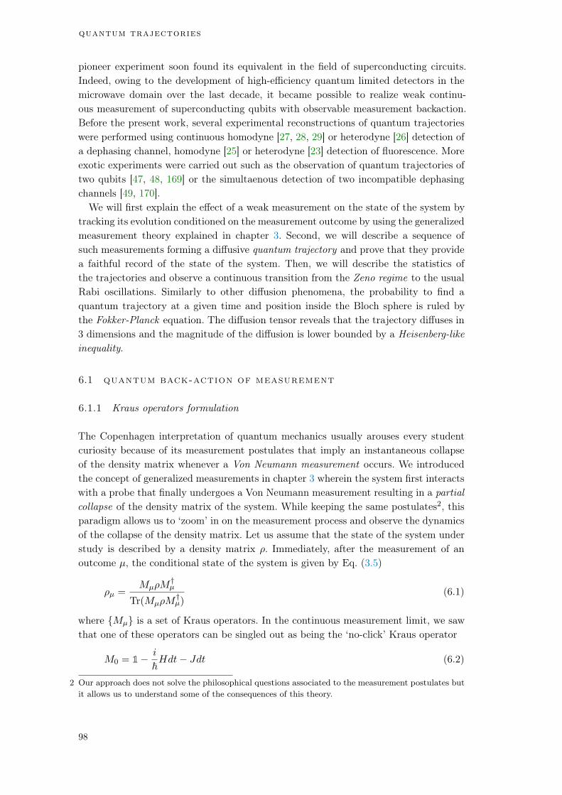
quantum trajectories
pioneer experiment soon found its equivalent in the field of superconducting circuits.Indeed, owing to the development of high-efficiency quantum limited detectors in themicrowave domain over the last decade, it became possible to realize weak continu-ous measurement of superconducting qubits with observable measurement backaction.Before the present work, several experimental reconstructions of quantum trajectorieswere performed using continuous homodyne [27, 28, 29] or heterodyne [26] detection ofa dephasing channel, homodyne [25] or heterodyne [23] detection of fluorescence. Moreexotic experiments were carried out such as the observation of quantum trajectories oftwo qubits [47, 48, 169] or the simultaenous detection of two incompatible dephasingchannels [49, 170].
We will first explain the effect of a weak measurement on the state of the system bytracking its evolution conditioned on the measurement outcome by using the generalizedmeasurement theory explained in chapter 3. Second, we will describe a sequence ofsuch measurements forming a diffusive quantum trajectory and prove that they providea faithful record of the state of the system. Then, we will describe the statistics ofthe trajectories and observe a continuous transition from the Zeno regime to the usualRabi oscillations. Similarly to other diffusion phenomena, the probability to find aquantum trajectory at a given time and position inside the Bloch sphere is ruled bythe Fokker-Planck equation. The diffusion tensor reveals that the trajectory diffuses in3 dimensions and the magnitude of the diffusion is lower bounded by a Heisenberg-likeinequality.
6.1 quantum back-action of measurement
6.1.1 Kraus operators formulation
The Copenhagen interpretation of quantum mechanics usually arouses every studentcuriosity because of its measurement postulates that imply an instantaneous collapseof the density matrix whenever a Von Neumann measurement occurs. We introducedthe concept of generalized measurements in chapter 3 wherein the system first interactswith a probe that finally undergoes a Von Neumann measurement resulting in a partialcollapse of the density matrix of the system. While keeping the same postulates2, thisparadigm allows us to ‘zoom’ in on the measurement process and observe the dynamicsof the collapse of the density matrix. Let us assume that the state of the system understudy is described by a density matrix . Immediately, after the measurement of anoutcome µ, the conditional state of the system is given by Eq. (3.5)
µ =MµM
†µ
Tr(MµM†µ)
(6.1)
where Mµ is a set of Kraus operators. In the continuous measurement limit, we sawthat one of these operators can be singled out as being the ‘no-click’ Kraus operator
M0 = 1 i
~Hdt Jdt (6.2)
2 Our approach does not solve the philosophical questions associated to the measurement postulates butit allows us to understand some of the consequences of this theory.
98
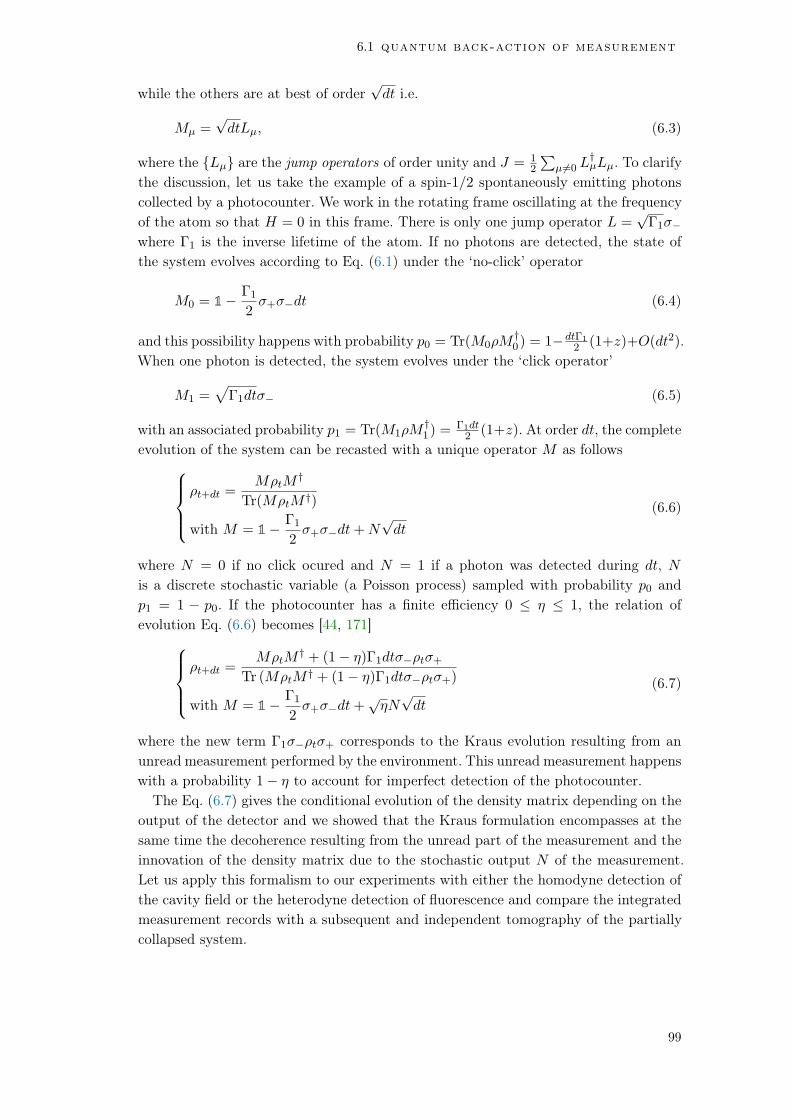
6.1 quantum back-action of measurement
while the others are at best of orderpdt i.e.
Mµ =pdtLµ, (6.3)
where the Lµ are the jump operators of order unity and J = 12
P
µ 6=0 L†µLµ. To clarify
the discussion, let us take the example of a spin-1/2 spontaneously emitting photonscollected by a photocounter. We work in the rotating frame oscillating at the frequencyof the atom so that H = 0 in this frame. There is only one jump operator L =
pΓ1
where Γ1 is the inverse lifetime of the atom. If no photons are detected, the state ofthe system evolves according to Eq. (6.1) under the ‘no-click’ operator
M0 = 1 Γ1
2+dt (6.4)
and this possibility happens with probability p0 = Tr(M0M†0) = 1 dtΓ1
2 (1+z)+O(dt2).When one photon is detected, the system evolves under the ‘click operator’
M1 =p
Γ1dt (6.5)
with an associated probability p1 = Tr(M1M†1) =
Γ1dt2 (1+z). At order dt, the complete
evolution of the system can be recasted with a unique operator M as follows8
>><
>>:
t+dt =MtM
†
Tr(MtM †)
with M = 1 Γ1
2+dt+N
pdt
(6.6)
where N = 0 if no click ocured and N = 1 if a photon was detected during dt, N
is a discrete stochastic variable (a Poisson process) sampled with probability p0 andp1 = 1 p0. If the photocounter has a finite efficiency 0 1, the relation ofevolution Eq. (6.6) becomes [44, 171]
8
>><
>>:
t+dt =MtM
† + (1 )Γ1dtt+Tr (MtM † + (1 )Γ1dtt+)
with M = 1 Γ1
2+dt+
pN
pdt
(6.7)
where the new term Γ1t+ corresponds to the Kraus evolution resulting from anunread measurement performed by the environment. This unread measurement happenswith a probability 1 to account for imperfect detection of the photocounter.
The Eq. (6.7) gives the conditional evolution of the density matrix depending on theoutput of the detector and we showed that the Kraus formulation encompasses at thesame time the decoherence resulting from the unread part of the measurement and theinnovation of the density matrix due to the stochastic output N of the measurement.Let us apply this formalism to our experiments with either the homodyne detection ofthe cavity field or the heterodyne detection of fluorescence and compare the integratedmeasurement records with a subsequent and independent tomography of the partiallycollapsed system.
99
quantum trajectories
6.1.2 Dispersive interaction
In the case of the continuous dispersive measurement, the jump operator is of the form
Lw =q
dΓd
2 z and the evolution of the state is given by the Kraus map8
>>>>>>>>>><
>>>>>>>>>>:
t+dt =K(t)
Tr(K(t))
where K(t) = MM † + (1 d)Γd
2zzdt
and M = 1 i
~H +
Γd
4
dt+
r
dΓd
2zw(t)dt
with the record w(t)dt =p
2dΓdztdt+ dWw(t)
. (6.8)
The expression of the measurement records comes from Eq. (3.23) and zt = Tr(zt) isthe z component of the Bloch vector. Note that we neglected any energy relaxation ofthe qubit and the pure dephasing of the artificial atom so Eq. (6.8) is valid for timesmuch smaller than T1 ' 15 µs and T' = 17.9 µs. In the case of an undriven system,the projections of Eq. (6.8) along the Bloch coordinates in the rotating frame of thequbit read
8
>><
>>:
dxt = Γdxtdtp
2dΓdxtztdWw(t)
dyt = Γdytdtp
2dΓdytztdWw(t)
dzt =p
2dΓd(1 z2t )dWw(t)
. (6.9)
In the actual experiments (Fig. 6.1), we integrate the record w(t)dt of Eq. (6.8)during a time T = 1 µs T1 and we compare it with an independent tomography(see Fig. 6.1 a) similarly to Murch et al. [27]. Owing to the stochastic nature of Eq. (6.9),integration and differentiation require the so-called Ito’s formula.
For a stochastic variable3Ht of the form
dHt = Atdt+BtdWt (6.10)
where dWt is a Brownian motion. The differential of a function f(Ht, t) that dependson the stochastic variable Ht is modified according to Ito’s formula
d(f(Ht, t)) =@f
@t(Ht, t)dt+
@f
@h(Ht, t)dHt +
1
2
@2f
@h2(Ht, t)B
2t dt (6.11)
From Eq. (6.11) we obtain
d(arctanh(zt)) =dzt
1 z2t+ 2ztdΓddt =
p
2dΓdw(t)dt (6.12)
that can be integrated between 0 and T to obtain the evolution of the z component ofthe qubit under measurement as a function of the integrated measurement record
arctanh(zT ) = arctanh(z0) +p
2dΓd
Z T
0w(t)dt. (6.13)
3 In our experiments, dHt plays the role of the increments of the Bloch coordinates (dxt, dyt, dzt).
100

6.1 quantum back-action of measurement
a.
b.
-40 -20 0 20 40
-1.0-0.50.0
0.5
1.0c. d.
Figure 6.1: a. Similarly to section 3.2. We amplify and detect the imaginary quadrature Im[aout]
of the cavity field leading to the measurement record w(t). The signal in the IQ
plane is squeezed along the Q quadrature before mixing with the local oscillator.
The measurement records encode the z component of the qubit state according to
Eq. (6.8). b. Pulse sequence. We initialize the qubit in hxi = 1 with a /2 pulse.
We integrate the measurement records w(t) during T = 1 µs, Q =R T
0w(t)dt. We
then perform a strong tomography of x, y or z at the end of the experiment.
c Back-action of the measurement on a qubit superposition state. The state of
the system is thrust toward |gi (south pole) or |ei (north pole) depending on the
sign and magnitude of the integrated record Q. d. We gather the experimental
realizations yielding the same integrated measurement record Q within ±1 mV and
we average the tomography results over 5 106 realizations. The signal measured
at the output of the refrigerator Q is amplified with a constant (cables attenuation,
LO power, ...) that was calibrated by measuring the output noise of the detection
setup (see section 6.2.3.1). The correlation between the integrated records and the
tomography behaves according to Eq. (6.15) (solid lines) with a quantum efficiency
d = 25% and measurement induced dephasing rate Γd = 0.95 µs in agreement
with independent calibrations. Note that the value of d is smaller than the one
used to unravel quantum trajectories in section 6.2 because the JPA was operated
at a different operating point.
101

quantum trajectories
Moreover we can infer the z component of the qubit because Sarlette and Rouchonshowed [172] that the dynamics of the density matrix is confined to an ellipsoid for thisdetection. The equation of the ellipsoid reads
x2t + y2t + bt(z2t 1) = 0 (6.14)
where = (1d)Γd and bt = b0et with b0 determined by the initial conditions. The
confinement of the dynamics to this manifold can be shown by direct calculation fromEq. (6.11) and a physical explanation is given in section 6.4.
From Eq. (6.13) and Eq. (6.14), we obtain that for a qubit initialized in the purestate |+i = (|gi+ |ei)/
p2 [27],
8
>>><
>>>:
xT =q
1 z2T eT
yT = 0
zT = tanhp
2dΓdQ
(6.15)
where Q =R T0 w(t)dt is the integrated measurement record.
We perform such an experiment in Fig. 6.1 a-b, we recall the detection setup and thepulse sequence for this measurement. The back-action of the weak measurement takesthe state of the qubit away from the equator and brings it toward one of the pointerstates of the measurement |gi or |ei depending on the integrated signal (Fig. 6.1 c).We can check the prediction of Eq. (6.15) to demonstrate that the Kraus operatorformalism (6.8) accurately describes the update of the quantum state conditioned onthe measurement record. This measurement provides a calibration of the quantumefficiency of the detection setup d = 25% in agreement with the method of section 3.2.
We demonstrated that we are able to observe the partial collapse of the wave functionunder the weak measurement of an observable. When the integrated signal is close tozero, no information was extracted on the state of the system. The density matrix staysclose to the equator. When the integrated signal is extremal, the qubit state collapsesin |gi or |ei. Increasing the measurement rate dΓd ! +1, the hyperbolic tangentof Eq. (6.15) can be replaced by a step function. We then recover the case of a VonNeumann measurement.
6.1.3 Measurement along the orthogonal quadrature
By changing the phase of the pump of the JPA, we can tune the squeezed quadrature ofthe amplifier. The information on the qubit state is encoded in the phase of the outgoingsignal that only contributes to the imaginary part of aout. This former quadrature isthus always chosen to readout a qubit. Conversely, the real part of the field does notdepend on the state of the qubit. It is thus discarded when performing a tomography. Inthis section, we demonstrate that the fluctuations of the real quadrature of the signalcarry the information about the back-action of the measurement induced dephasing[27].
102

6.1 quantum back-action of measurement
The jump operator of the problem is Lw0 = iLw = iq
dΓd
2 z. The projected dynamicsreads
8
>><
>>:
dxt = Γdxtdt+p
2dΓdytdWw(t)
dyt = Γdytdt+p
2dΓdxtdWw(t)
dzt = 0
(6.16)
with the measurement record
w0(t)dt = dWw0(t). (6.17)
Note that in this case, the total output signal of the detection setup corresponds toan offset signal
qn
2+2 (projection along the Q axis of the mean of the distributions
in Fig. 6.2 a) with n the average number of photons stored inside the cavity plusthe measurement record (6.17) that contains noise alone. This case is very interestingbecause the measurement record (6.17) does not depend on but still induces a back-action on the qubit state. The integrated record allows us to track the evolution ofthe qubit state according to Eq. (6.16). This measurement leads to a diffusive behaviorof the qubit state along the equator of the Bloch sphere (Fig. 6.2 c). It can even becorrected by feedback if one wants to stabilize a given state [28].
Similarly to the previous case, the state of the qubit is confined to a deterministiccircle [172] at a constant z altitude in the Bloch sphere. Besides,
x2t + y2t = et, (6.18)
where = (1 )Γd is the measurement induced dephasing rate corresponding to theunmonitored part of the cavity field. A physical explanation of this property is givenin section 6.4. Let us use Ito rule (6.11) and differentiate
8
>>><
>>>:
d(arccos(xt)) =dΓdxtdtp
1 x2t
1 y2t1 x2t
p2ΓmytdWw0(t)p
1 x2t
d(arcsin(yt)) = dΓdytdtp
1 y2t
1 x2t1 y2t
p2ΓmxtdWw0(t)p
1 y2t
(6.19)
where xt = etxt and yt = etyt. Using Eq. (6.18), the expression boils down to(
d(arccos(etxt)) = p
2dΓddWw0(t)
d(arcsin(etyt)) =p
2dΓddWw0(t). (6.20)
We obtain the evolution of the Bloch coordinate between 0 and T as a function ofthe integrated measurement record, for a qubit starting in (|gi+ |ei)/
p2
8
<
:
xT = cosp
2dΓdI
eT
yT = sinp
2dΓdI
eT(6.21)
where I =R T0 w0(t)dt is the integrated measurement record.
Histograms of the integrated measurement (Fig. 6.2) records reveal a clear correlationwith the final tomography according to Eq. (6.21). We find a corresponding quantumefficiency of d = 24% with the same operating point as in Fig. 6.1.
103

quantum trajectories
a.
b.
c. d.
-40 -20 0 20 40
-0.4-0.20.0
0.2
0.4
Figure 6.2: a. We amplify and detect the quadrature Re[aout] of the cavity field leading to
the measurement record w0(t). The signal in the IQ plane is squeezed along the
I quadrature before mixing with the local oscillator. The measurement records
do not depend on the qubit state according to Eq. (6.17) but its noise contains
the information on the dephasing of the qubit. Note that we do not take into
consideration the offset signal q
nκκ2+χ2 in the IQ plane so that w0(t) has a zero
average. b. Pulse sequence. We initialize the qubit in hxi = 1 with a /2 pulse.
We integrate the measurement records w0(t) during T = 1 µs, I =R T
0w0(t)dt. We
perform a strong tomography of x, y or z at the end of the experiment. c Back-
action of the measurement on a qubit superposition state. The state of the system
picks up a random phase that depends on the measurement record. d. We gather the
experimental realizations yielding the same integrated measurement record I and
we average the tomography results over 5 106 realizations. The signal measured
at the output of the refrigerator I is amplified by a constant that was calibrated
by measuring the output noise of the detection setup (see section 6.2.3.1). The
correlation between the integrated records and the tomography behaves according
to Eq. (6.21) (solid lines) with a quantum efficiency d = 24% and measurement
induced dephasing rate Γd = 0.95 µs in agreement with independent calibrations.
104

6.1 quantum back-action of measurement
6.1.4 Fluorescence signal
One can also investigate the back-action of the fluorescence measurement. Following[85], we obtain integrable quantities for the monitoring of energy relaxation. In thiscase, the evolution of the density matrix is related to integrated weighted signal andnot to the raw integrated signals. The problem is described by two jump operatorsLu =
p
Γ1/2 and Lv = iLu. Similarly to Eq. (6.8), we can write the incrementalevolution of the density matrix as a function of Kraus operators
8
>>>>><
>>>>>:
t+dt =K(t)
Tr(K(t))
where K(t) = MM † + (1 f )Γ1(+)dt
and M = 1 (i
~H +
Γ1
2+)dt+
r
fΓ1
2(u(t) + iv(t))dt
. (6.22)
with the records8
>><
>>:
u(t)dt =
r
fΓ1
2xtdt+ dWu(t)
v(t)dt =
r
fΓ1
2ytdt+ dWv(t)
. (6.23)
In the case H = 0, projecting Eq. (6.22) along the Bloch coordinates yields
8
>>>>>>><
>>>>>>>:
dxt = Γ1
2xtdt+
r
fΓ1
2
(1 + zt x2t )dWu(t) xtytdWv(t)
dyt = Γ1
2ytdt+
r
fΓ1
2
(1 + zt y2t )dWv(t) xtytdWu(t)
dzt = Γ1(1 + zt)dtr
fΓ1
2(1 + z)(xdWu(t) + ydWv(t))
(6.24)
Remarkably, the dynamics of the quantum state predicted by Eq. (6.24) is restrictedto the surface of a deterministic spheroid going through the south pole of the Blochsphere [23, 172]
ct(x2t + y2t ) + c2t
zt + 1 1
ct
2
= 1 (6.25)
where ct = f+(c(0))eΓ1t and c(0) is determined by the initial condition. We workedin the presence of a parasitic pure dephasing of rate Γ' ' (27 µs)1 that leads to anadditional decoherence dynamics dxt = Γ'xtdt and dyt = Γ'ytdt. Using Ito rule
8
>>><
>>>:
d
xt
1 + zt
=
Γ1
2 Γ'
xt
1 + zt+fΓ1
2xt +
r
fΓ1
2dWu
=
Γ1
2 Γ'
xt
1 + zt+
r
fΓ1
2u(t)dt
. (6.26)
105
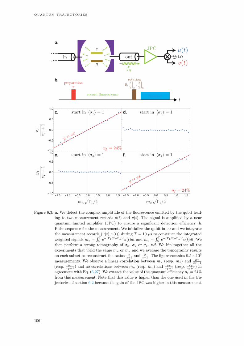
quantum trajectories
a.
-1.0-0.50.0
0.5
1.0
-1.5 -1.0 -0.5 0.0 0.5 1.0 1.5-1.0-0.50.0
0.5
1.0
1.5 -1.0 -0.5 0.0 0.5 1.0 1.5-
c. d.
e. f.
b.
Figure 6.3: a. We detect the complex amplitude of the fluorescence emitted by the qubit lead-
ing to two measurement records u(t) and v(t). The signal is amplified by a near
quantum limited amplifier (JPC) to ensure a significant detection efficiency. b.
Pulse sequence for the measurement. We initialize the qubit in |ei and we integrate
the measurement records (u(t), v(t)) during T = 10 µs to construct the integrated
weighted signals mu =R T
0e(Γ1/2Γϕ)tu(t)dt and mv =
R T
0e(Γ1/2Γϕ)tv(t)dt. We
then perform a strong tomography of x, y or z. c-f. We bin together all the
experiments that yield the same mu or mv and we average the tomography results
on each subset to reconstruct the ratios xz+1 and y
z+1 . The figure contains 9.5 105
measurements. We observe a linear correlation between mu (resp. mv) and xT
zT+1
(resp. yT
zT+1 ) and no correlations between mu (resp. mv) and yT
zT+1 (resp. xT
zT+1 ) in
agreement with Eq. (6.27). We extract the value of the quantum efficiency f = 24%
from this measurement. Note that this value is higher than the one used in the tra-
jectories of section 6.2 because the gain of the JPC was higher in this measurement.
106

6.2 quantum trajectories
The quantity yt/1 + zt can also be differentiated. We obtain the following result fora qubit starting in hzi = 1
8
>>><
>>>:
e(Γ12Γϕ)T x(T )
z(T ) + 1=
r
fΓ1
2mu
e(Γ12Γϕ)T y(T )
z(T ) + 1=
r
fΓ1
2mv
(6.27)
where mu =R T0 e(Γ1/2Γϕ)tu(t)dt and mv =
R T0 e(Γ1/2Γϕ)tv(t)dt are the integrated
weighted signals.The predicted Bloch coordinates xt = Tr[xt], yt = Tr[yt] and zt = Tr[zt] are
not independently measurable in a single realization of an experiment. Let us select aset of trajectories sharing a given mu. Every trajectory k as the same xk
1+zkratio which
is also equal to x1+z where . denotes the average of the set of trajectory of equal mu.
We can thus repeat the experiment and carry alternatively a strong measurement ofeither x, y or z and compute the x
1+z ratio of all trajectories that led to the samemu. In Fig. 6.3, we record the fluorescence signal of a qubit initialized in hxi = 1 forT = 10 µs. We sort the trajectories according to the values of mu and mv calculatedby integration of the measurement records. We observe a linear correlation betweenmu and x
z+1 and between mv and yz+1 validating the Kraus operator formalism to
predict the evolution of a relaxing qubit undergoing an heterodyne measurement. Themeasurement is a calibration of the quantum efficiency of detection, here f = 24%.
6.2 quantum trajectories
6.2.1 Repeated Kraus map and Markov chain
In the previous section, we saw measurement ‘in action’ and we demonstrated thatthe Kraus formalism of equations (6.7,6.8,6.22) faithfully predicts the update of thedensity matrix conditioned to the information written in an observer’s memory duringa single measurement of duration T . Let us extend this formalism to an arbitrary set ofjump operators Lµ associated to the detection efficiencies µ characterizing everydecoherence channel of the system.
The incremental evolution of a quantum state of a monitored open quantum systemreads
8
>>>>>>>>><
>>>>>>>>>:
t+dt =Ky(t)(t)
Tr(Ky(t)(t))
with Ky(t)(t) = My(t)tM†y(t) +
X
µ 6=0
(1 µ)dtLµtL†µ
and My(t) = 1
0
@i
~H +
X
µ 6=0
L†µLµ/2
1
A dt+X
µ 6=0
pµLµyµ(t)dt
(6.28)
The associated measurement records read
yµ(t)dt =pµTr(Lµ+ L†
µ)dt+ dWµ(t). (6.29)
107

quantum trajectories
and y(t) = (yµ(t))µ is the vector of the measurement records at time t. The super-operator K is called a partial4 Kraus map. We recall the properties of the Wienerprocesses Wµ in Ito formalism
(
E[dWµ(t)] = 0
dWµ(t)2 = dt
. (6.30)
Repeating a series of such measurements5 yields a succession of outcomes y(0), y(dt), y(2dt), ...and at each time step the density matrix is updated in agreement with
ndt ! ndt+dt = (n+1)dt =Ky(ndt)(ndt)
Tr(Ky(ndt)(ndt))(6.31)
Under Markov assumption, the successive evolutions (6.31) are independent andstochastic specifying a Markov chain6 on the density matrix called quantum trajec-tory. A quantum trajectory is the time evolution of the density matrix of a systemmonitored by an observer7 conditioned on the realization of the measurement records.
6.2.2 The stochastic master equation
At first order in dt, the partial Kraus map of Eq. (6.28) reads
Ky(t)(t) = t i
~[H, t]dt+
X
µ
dt(LµtL†µ L†
µLµ
2t t
L†µLµ
2)
+X
µ
pµ(Lµt + tL
†µ)yµ(t)dt.
(6.32)
And since Tr(Ky(t)(t)) = 1+P
µpµTr(Lµt+tL
†µ)yµ(t)dt. The normalisation factor
can be approximated at order dt by
1
Tr(Ky(t)(t))= 1
X
µ
pµTr(Lµt+tL
†µ)yµ(t)dt+
X
µ
µTr(Lµt+tL†µ)
2dt. (6.33)
By combining Eq. (7.8) and Eq. (7.9), we obtain the so-called stochastic master equation(SME)
dt = i
~[H, t]dt+
mX
i=1
Di(t)dt+mX
i=1
piMi(t)dWi(t) (6.34)
where the Lindblad super-operator is Di(t) = LitL†i 1
2tL†iLi 1
2L†iLit, the innova-
tion super-operator is Mi(t) = Lit + tL†i Tr(Lit + tL
†i )t and the measurement
records are given by Eq. (6.29).
4 A partial Kraus map is not trace preserving in general Tr(K(ρ)) Tr(ρ) contrary to a Kraus map.5 This formalism can be extended to an arbitrary sequence of measurements of unequal duration
T1, T2, T3, ...
6 See for instance [108, 173] for an introduction on the subject.7 The quantum trajectory is observer-dependent. The dynamics of the system is defined by its Hamilto-
nian, the set of jump operators Lµ and the initial condition. A class of observer is specified by theset of measurement efficiencies ηµ associated to each information channel.
108
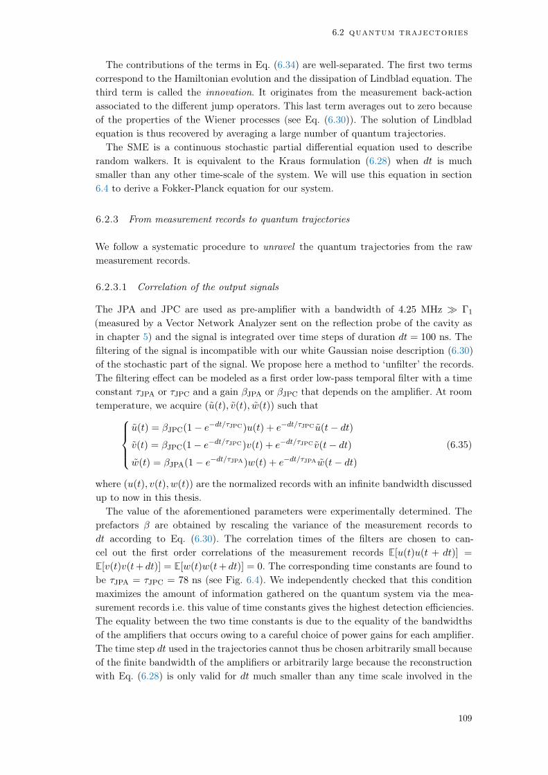
6.2 quantum trajectories
The contributions of the terms in Eq. (6.34) are well-separated. The first two termscorrespond to the Hamiltonian evolution and the dissipation of Lindblad equation. Thethird term is called the innovation. It originates from the measurement back-actionassociated to the different jump operators. This last term averages out to zero becauseof the properties of the Wiener processes (see Eq. (6.30)). The solution of Lindbladequation is thus recovered by averaging a large number of quantum trajectories.
The SME is a continuous stochastic partial differential equation used to describerandom walkers. It is equivalent to the Kraus formulation (6.28) when dt is muchsmaller than any other time-scale of the system. We will use this equation in section6.4 to derive a Fokker-Planck equation for our system.
6.2.3 From measurement records to quantum trajectories
We follow a systematic procedure to unravel the quantum trajectories from the rawmeasurement records.
6.2.3.1 Correlation of the output signals
The JPA and JPC are used as pre-amplifier with a bandwidth of 4.25 MHz Γ1
(measured by a Vector Network Analyzer sent on the reflection probe of the cavity asin chapter 5) and the signal is integrated over time steps of duration dt = 100 ns. Thefiltering of the signal is incompatible with our white Gaussian noise description (6.30)of the stochastic part of the signal. We propose here a method to ‘unfilter’ the records.The filtering effect can be modeled as a first order low-pass temporal filter with a timeconstant JPA or JPC and a gain JPA or JPC that depends on the amplifier. At roomtemperature, we acquire (u(t), v(t), w(t)) such that
8
>><
>>:
u(t) = JPC(1 edt/JPC)u(t) + edt/JPC u(t dt)
v(t) = JPC(1 edt/JPC)v(t) + edt/JPC v(t dt)
w(t) = JPA(1 edt/JPA)w(t) + edt/JPAw(t dt)
(6.35)
where (u(t), v(t), w(t)) are the normalized records with an infinite bandwidth discussedup to now in this thesis.
The value of the aforementioned parameters were experimentally determined. Theprefactors are obtained by rescaling the variance of the measurement records todt according to Eq. (6.30). The correlation times of the filters are chosen to can-cel out the first order correlations of the measurement records E[u(t)u(t + dt)] =
E[v(t)v(t+ dt)] = E[w(t)w(t+ dt)] = 0. The corresponding time constants are found tobe JPA = JPC = 78 ns (see Fig. 6.4). We independently checked that this conditionmaximizes the amount of information gathered on the quantum system via the mea-surement records i.e. this value of time constants gives the highest detection efficiencies.The equality between the two time constants is due to the equality of the bandwidthsof the amplifiers that occurs owing to a careful choice of power gains for each amplifier.The time step dt used in the trajectories cannot thus be chosen arbitrarily small becauseof the finite bandwidth of the amplifiers or arbitrarily large because the reconstructionwith Eq. (6.28) is only valid for dt much smaller than any time scale involved in the
109

quantum trajectories
0
10
-10
-20
-30
-40
-50
50 100 150 2000 78
Figure 6.4: Non normalized experimental correlations between two consecutive unfiltered mea-
surement records before normalizing their variance to dt as a function of the time
scale of Eq. (6.35). The parameters JPA = JPC = 78 ns (green dashed line) were
found to cancel the autocorrelation of the signals induced by the finite bandwidth
of the amplifiers.
experiment. Our choice dt = 100 ns was the smallest achievable time step compatiblewith the bandwidth of the amplifiers. The unfiltered and rescaled measurement recordsare used to reconstruct all the trajectories presented in this thesis.
6.2.3.2 Unravelling the trajectory
We model our system with four jump operators Lu =q
Γ12 , Lv = iLu, Lw =
qdΓd
2 z
and L' =q
Γϕ
2 z. The fourth jump operator takes into account the unread (' = 0)pure dephasing8 of the qubit so that the total decoherence rate of the system is Γ2 =Γ12 + Γ' + Γd. The measurement record-dependent evolution reads
8
>>>>>>><
>>>>>>>:
t+dt =Ky(t)(t)
Tr(Ky(t)(t))
with Ky(t)(t) = My(t)tM†y(t) + (1 f )dtΓ1+ + (1 d)dt
Γd
2zz
and My(t) = 1
iH
~+
Γ1
2+ +
Γd + Γ'
4
dt+
r
fΓ1
2(u(t) + iv(t))dt+
r
dΓd
2zw(t)dt
.
(6.36)
The system is driven by an Hamiltonian of the form H = ~Ω
2 y where Ω is the Rabifrequency. All the parameters that enter Eq. (6.36) are determined by independent
8 Γϕ is the residual dephasing rate of the qubit when the cavity is not populated.
110
6.2 quantum trajectories
measurements and we check that the average evolution9 is faithfully described by theLindblad equation with the corresponding parameters.
1 2 3 4 5-10
-5
0
5
10a. b.
Figure 6.5: A typical 5 µs-long tracking of a quantum state. a. Raw (not normalized) mea-
surement records u(t) (blue), v(t) (red) and w(t) (yellow) as a function of time
for one realization of the experiment. These records feed Eq. (6.36) with the pa-
rameters Γ1 = (15 µs)1, Γd = (0.9 µs)1, Γϕ = (17.9 µs)1, Ω/2 = 5.2 µs and
(f , d) = (14%, 34%). The records are very noisy but Eq. (6.36) acts as a filter that
leads to the trajectory represented in the Bloch sphere in b.
In Fig. 6.5, we give Bloch sphere representation of a 5 µs-long quantum trajectory.The measurement records are dominated by noise but Eq. (6.36) acts as a Bayesianfilter leading to a diffusive trajectory. The trajectory is oscillating around the y axisbecause of the drive described by the Hamiltonian.
6.2.4 Validation by an independent tomography
Quantum trajectories are physically meaningful if and only if they can be used to predictthe distribution of outcomes of any future measurement performed of the system. Thevalidity of the reconstructed trajectories can be tested by post-selecting an ensemble ofrealizations of the experiment for which the trajectory predicts a given value x(T ) =
xtraj at a time T . If the trajectories are valid, then a strong measurement of x at timeT should give xtraj on average on this post-selected ensemble of realizations. In practice,we compare the prediction of the quantum trajectories with a strong measurement byselecting all the trajectories of a large ensemble that ends up in some slice of the Blochsphere (see Fig. 6.6). An example of 4 trajectories ending up with 0.74 < xtraj < 0.76
are depicted on Fig. 6.6 d. Here, the average over the strong x measurement yields avalue ' 0.75.
9 We recall that the raw average of the measurement records is a full quantum tomography of the system(see section 3.4).
111
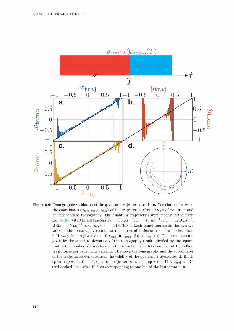
quantum trajectories
a. b.
c. d.
Figure 6.6: Tomographic validation of the quantum trajectories. a. b. c. Correlations between
the coordinates (xtraj, ytraj, ztraj) of the trajectories after 19.8 µs of evolution and
an independent tomography. The quantum trajectories were reconstructed from
Eq. (6.36) with the parameters Γ1 = (15 µs)1, Γd = (5 µs)1, Γϕ = (17.9 µs)1,
Ω/2 = (5 µs)1 and (f , d) = (14%, 34%). Each panel represents the average
value of the tomography results for the subset of trajectories ending up less than
0.01 away from a given value of xtraj (a), ytraj (b) or ztraj (c). The error bars are
given by the standard deviation of the tomography results divided by the square
root of the number of trajectories in the subset out of a total number of 1.5 million
trajectories per panel. The agreement between the tomography and the coordinates
of the trajectories demonstrates the validity of the quantum trajectories. d. Bloch
sphere representation of 4 quantum trajectories that end up with 0.74 < xtraj < 0.76
(red dashed line) after 19.8 µs corresponding to one bin of the histogram in a.
112
6.2 quantum trajectories
We have checked for any value of xtraj (Fig. 6.6 a), ytraj (Fig. 6.6 b) and ztraj (Fig. 6.6c), and for 30 representative values of measurement strength and drive that the trajec-tories predict accurately the tomography results. However, in the presence of a largedrive Ω 1/dt or a large measurement rate Γd 1/dt, the unravelling (6.36) is nolonger valid and large deviations are observed between the reconstructed trajectoriesand the independent tomography.
6.2.5 Parameter estimation
In this section, we show that the parameters of the filter (6.36) can be inferred in aself-consistant manner from the measurement records themselves. It was already demon-strated in our group by Six et al with a maximum likelihood estimation in the frame-work of hidden Markov problems [174]. We propose instead a new empirical methodthat rely on the validation of the trajectories by an independent tomography. We applythe stochastic filter (6.36) for various values of the parameter that we want to esti-mate. Only the correct value provides valid quantum trajectories in agreement witha subsequent tomography. The time constants entering Eq. (6.36) can be estimatedby comparing the average evolution of the system with the solution of the Lindbladequation or by Rabi and Ramsey calibrations, which is not the case for the quantumefficiencies f and d. We thus apply this method to estime them precisely.
In Fig. 6.7, the trajectories are reconstructed for several values of f and d and theircoordinates (xtraj,ytraj,ztraj) are statistically compared to an independent tomography(similarly to Fig. 6.6). The results of the trajectories and the tomography are in agree-ment only for the correct values of the efficiencies. In practice, there exists a correlationbetween the coordinates of the trajectory and the measurement records in the othercases that is approximately linear with a slope different from 1. We extract the slope ofthe correlation histograms by linear regression for the different values of the efficiencies.We find that the agreement is verified for efficiencies f = 0.14 and d = 0.34 withina confidence interval of ±0.01 for any values of the amplitude drive and measurementinduced dephasing rate.
113

quantum trajectories
a1.
-1.0 -0.5 0.0 0.5 1.0-1.0-0.50.0
0.5
1.0-1.0-0.50.0
0.5
1.01.0 -0.5 0.0 0.5 1.0
0.05 0.10 0.15 0.20 0.25
1.0
1.2
1.4
1.6
1.8
slopeoflinearregression
-1.0 -0.5 0.0 0.5 1.0
-0.50.0
0.5
1.0
1.0-
0.8
b1.
c1. d1.
a2. b2.
c2. d2.
-1.0-0.50.0
0.5
1.01.0 -0.5 0.0 0.5 1.0-1.0 -0.5 0.0 0.5 1.0
-0.50.0
0.5
1.0
1.0-
-1.0 -0.5 0.0 0.5 1.0-1.0-0.50.0
0.5
1.0
0.25 0.30 0.35 0.40 0.45
0.85
0.90
0.95
1.00
1.05
1.10
1.15
slopeoflinearregression
Figure 6.7: Correlations between the coordinates (xtraj,ytraj,ztraj) of the trajectories after
19.8 µs of evolution and an independent tomography on the dataset correspond-
ing to Γ1 = (15 µs)1, Γd = (5 µs)1, Γϕ = (17.9 µs)1 and Ω/2 = (2.0 µs)1.
In Fig. a1,b1,c1 the sole output of the fluorescence records is used to reconstruct
the trajectories (d = 0) and f takes 3 different values in Eq. (6.36). Incorrect
values of f lead to a deviation from a slope one line (in black). Similarly f is
set to 0 in a2,b2,c2 and three values of d are tested. Note that because of the
structure of the dispersive measurement back-action, all the dynamics of the qubit
is confined in the x z plane with this sole detection thus ytraj = 0 at all times in
agreement with Fig. 6.1. In Fig. d1 and d2 the slopes of the correlation histograms
are extracted by linear regression for the different values of f and d used each
time in Eq. (6.36). The values f = 0.14 and d = 0.34 (green solid lines) are found
by this method with a precision ±0.01 (green dashed lines).
114
6.3 trajectories statistics
6.3 trajectories statistics
A quantum trajectory is a stochastic process corresponding to a random walk in theBloch sphere. The inherent back-action of a quantum measurement is thus better dis-cussed by representing distributions of states at a given time [27, 175, 176, 23, 24, 49] ordistributions of trajectories for a given duration [175, 177, 25, 169, 178]. Before repre-senting the statistics of our trajectories, we observe the impact of the values of the Rabifrequency and measurement induced dephasing rate on the average trajectory. Then,we compare the statistics obtained by different observers in two characteristic regimes.Finally, we advertise an online animated viewer created for this thesis to observe thetrajectories in all regimes from the viewpoints of the different observers.
6.3.1 Different regimes
By varying the drive amplitudes at the cavity and qubit transition frequencies, weare able to reach a variety of regimes corresponding to different values of Ω/Γ1 andΓd/Γ1. The timescales Γ1
1 and Γ1' are fixed because they characterize the lifetimes of
the energy and coherences of the undriven qubit. The measurement induced dephasingrate Γd can be tuned arbitrarily10 as it is proportional to the drive power at fc. The Rabifrequency Ω is arbitrarily tunable as well as it is proportional to the drive amplitudeat fq.
As we showed in section 3.4, the raw average of the measurement records is a fullquantum tomography of the qubit in time. In this section, we reveal the impact of theconfiguration of parameters on the average trajectory. Let us exemplify the variety ofobtainable regimes with two configurations of the input drive: one in the regime ofunderdamped Rabi oscillations (Fig. 6.8 a) and another one in the regime of strongdispersive measurement rate, the so-called Zeno regime [30, 31] (over-damped oscilla-tions of Fig. 6.8 b). In both cases, the qubit is initialized in the ground state and aRabi rotation around y is applied. The effect of decoherence under a strong Rabi drivecorresponds to an average loss of purity Tr(2) = 1
2(1+ x2 + y2 + z2) that can be seenas a decreasing distance of the mean trajectory from the center of the Bloch spherewhen time increases. In the long time limit, the state converges towards the centerof the Bloch sphere, which is the maximally mixed state or most entropic state of thesphere. In Fig. 6.8 a, the qubit state evolves with underdamped oscillations because thedecoherence rates are much smaller than the Rabi frequency Γ1,Γd Ω
2 . In contrast,in Fig. 6.8 a the qubit state endures over-damped oscillations because Γ1,
Ω
2 Γd.The circular motion is blocked by the presence of a large dephasing channel and theaverage trajectory quickly reaches its steady state.
10 For high values of Γd dt1, Eq. (6.36) is not valid. When reaching a critical number of photons(around 100 photons in our system), the transmon is driven into highly excited states and it is nolonger a qubit. This is the high power readout regime (see introduction of chapter 3).
115

quantum trajectories
a. b.
t t
Figure 6.8: Direct averaging of the three measurement records in the under-damped Rabi
oscillation regime and in the over-damped Zeno regime. a. Dots: Rescaled av-
erage of the measurement records u(t) = u(t)/p
fΓ1/2, v(t) = v(t)/p
fΓ1/2
and w(t) = w(t)/p2dΓd for 1.5 106 realizations of an experiment where the
qubit starts in |gi at time 0 and is driven so that it rotates at a Rabi frequency
Ω/2 = (2 µs)1 around y and endures a measurement induced dephasing rate
Γd = (5 µs)1 . Lines: Calculated coordinates of the Bloch vector x(t), y(t) and
z(t) from the master equation (6.36) with d,f = 0). b. Same figure in the Zeno
regime with a drive such that Ω/2 = (16 µs)1 and Γd = (0.9 µs)1.
116
6.3 trajectories statistics
6.3.2 Zeno dynamics - Interplay between detectors
We first focus on the Zeno regime of Fig. 6.8 b because the competition between theback-action of fluorescence measurement and dispersive measurement can be better ob-served when decoherence dominates the dynamics. We reconstruct an ensemble of 1.5million experiments and obtain the statistics of the trajectories. In Fig. 6.9, we showthe distributions of qubit states in color at a long time = 6.5 µs after which the distri-bution is close to its steady state while the qubit is both Rabi driven and dispersivelymeasured at a strong measurement rate. The average over this set of trajectories givesthe average trajectory (black solid line). The finite spread of the distribution aroundthe average trajectory is only due to the measurement back-action corresponding tothe stochastic term in Eq. (6.34). The trajectories are determined using three sets ofmeasurement records: dispersive only w(t) (Fig. a b c), fluorescence only u(t), v(t)
(Fig. d e f) or both (Fig. g h i). These three cases correspond to three different ob-servers that access different quantum states based on their records during the samerealization of the experiment. The uniqueness of perception of the three observers hasits roots in the records stored in the observer’s memory and it leads to the distinctstatistics of Fig. 6.9. In practice, we retrieve the information from both detectors for ev-ery experiment and we discard a part of this information in hindsight by setting f = 0
or d = 0 in Eq. (6.36) to reconstruct the trajectories, which is exactly equivalent toremoving the unread detector.
The Zeno effect leads to the damping of the Rabi oscillations and the average trajec-tory (solid line) quickly reaches its steady state. The average trajectory is the same forevery observer because it is predicted to be independent of the measurement records(average of Eq. (6.34)). Interestingly, while the average trajectory stays in the x z
plane with hyi = 0 (similarly to Fig. 6.8 b), the back-action of the fluorescence mea-surement leads to a nonzero spread (back-action) in the y direction of the Bloch sphere(Fig. 6.9 d). This is in stark constrast with the dispersive measurement alone that doesnot provide any back-action towards the y direction of the Bloch sphere(Fig. 6.9 a)so that the qubit states keeps a zero y component during its evolution. In the caseof fluorescence, in the long time, the combined action of Rabi drive and fluorescencemeasurement back-action leads to a uniform spread of the qubit state close to the mostentropic state 1/2 at the center of the sphere (Fig. 6.9 d e f). The qubit states spana small Bloch sphere composed of very unpure states revealing only a small amountof information on the state of the system because of the large measurement induceddephasing rate created by the strong dispersive measurement.
When the dispersive measurement is recorded (Fig. 6.9 a b c), a trajectory corre-sponding to a single realization of the experiment experiences a series of stochasticjumps between two areas of the Bloch sphere that are close to the two eigenstatesof the z measurement operator. In the distribution of states, this leads to two areaswith high probability of occupation near the poles of the Bloch sphere. The dispersivemeasurement records can thus reveal that the state of the qubit was either close to|gi or |ei revealing almost one bit of information on the qubit. These two areas canbe interpreted as zones frozen by the Zeno effect. The rest of the Bloch sphere is still
117

quantum trajectories
a. b. c.
d. e. f.
i.h.g.
dispersive measurement
fluorescence measurement
dispersive and fluorescence measurement
# trajectories1 10 100 1000
Figure 6.9: Impact of the type of detector on the distribution of quantum states in the Zeno
regime. a,b,c Marginal distribution in the x y (a), x z (b) and y z (c)
planes of the Bloch sphere of the qubit states τ corresponding to 1.5 millions of
measurement records at the cavity frequency only w(t) from time t between 0 and
= 6.5 µs. The information about u(t), v(t) is here discarded (by setting f = 0).
All panels in the figure correspond to the Zeno regime with Ω/2 = (5.2 µs)1 and
Γd = (0.9 µs)1. The boundary of the Bloch sphere is represented as a black circle
and the average quantum trajectory as a solid line. d,e,f Case where the states
are conditioned on fluorescence records u(t), v(t) instead while discarding the
information on w(t) (d = 0). g,h,i Case where the states are conditioned on
both fluorescence and dispersive measurement records u(t), v(t), w(t).
118
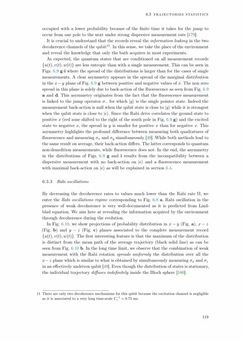
6.3 trajectories statistics
occupied with a lower probability because of the finite time it takes for the jump tooccur from one pole to the next under strong dispersive measurement rate [179].
It is crucial to understand that the records reveal the information leaking in the twodecoherence channels of the qubit11. In this sense, we take the place of the environmentand reveal the knowledge that only the bath acquires in most experiments.
As expected, the quantum states that are conditioned on all measurement recordsu(t), v(t), w(t) are less entropic than with a single measurement. This can be seen inFigs. 6.9 g-i where the spread of the distributions is larger than for the cases of singlemeasurements. A clear asymmetry appears in the spread of the marginal distributionin the xy plane of Fig. 6.9 g between positive and negative values of x. The non zerospread in this plane is solely due to back-action of the fluorescence as seen from Fig. 6.9a and d. This asymmetry originates from the fact that the fluorescence measurementis linked to the jump operator for which |gi is the single pointer state. Indeed themeasurement back-action is null when the qubit state is close to |gi while it is strongestwhen the qubit state is close to |ei. Since the Rabi drive correlates the ground state topositive x (red zone shifted to the right of the south pole in Fig. 6.9 g) and the excitedstate to negative x, the spread in y is smaller for positive x than for negative x. Thisasymmetry highlights the profound difference between measuring both quadratures offluorescence and measuring x and y simultaneously [49]. While both methods lead tothe same result on average, their back-action differs. The latter corresponds to quantumnon-demolition measurements, while fluorescence does not. In the end, the asymmetryin the distributions of Figs. 6.9 g and i results from the incompatibility between adispersive measurement with no back-action on |ei and a fluorescence measurementwith maximal back-action on |ei as will be explained in section 6.4.
6.3.3 Rabi oscillations
By decreasing the decoherence rates to values much lower than the Rabi rate Ω, weenter the Rabi oscillations regime corresponding to Fig. 6.8 a. Rabi oscillation in thepresence of weak decoherence is very well-documented as it is predicted from Lind-blad equation. We aim here at revealing the information acquired by the environmentthrough decoherence during the evolution.
In Fig. 6.10, we show projections of probability distribution in x y (Fig. a), x z
(Fig. b) and y z (Fig. c) planes associated to the complete measurement recordu(t), v(t), w(t). The first interesting feature is that the maximum of the distributionis distinct from the mean path of the average trajectory (black solid line) as can beseen from Fig. 6.10 b. In the long time limit, we observe that the combination of weakmeasurement with the Rabi rotation spreads uniformly the distribution over all thexz plane which is similar to what is obtained by simultaneously measuring x and zin an effectively undriven qubit [49]. Even though the distribution of states is stationary,the individual trajectory diffuses indefinitely inside the Bloch sphere [180].
11 There are only two decoherence mechanisms for this qubit because the excitation channel is negligibleas it is associated to a very long time-scale Γ
1" = 0.75 ms.
119
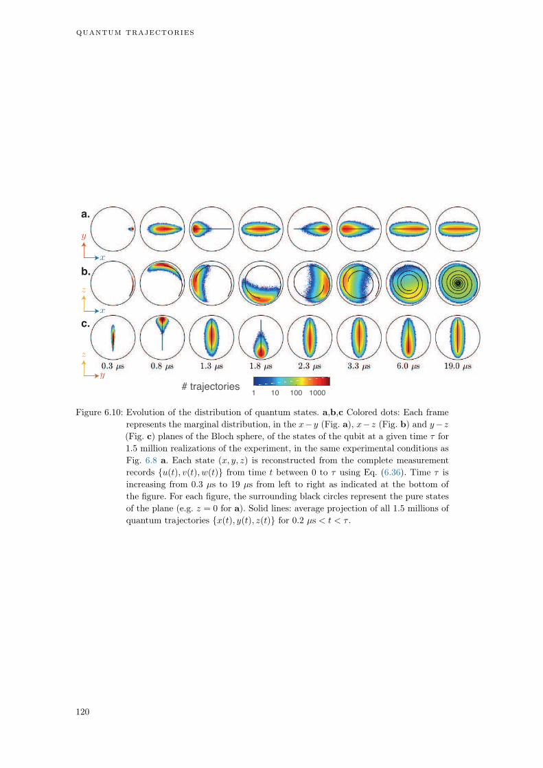
quantum trajectories
a.
b.
c.
# trajectories1 10 100 1000
Figure 6.10: Evolution of the distribution of quantum states. a,b,c Colored dots: Each frame
represents the marginal distribution, in the xy (Fig. a), x z (Fig. b) and y z
(Fig. c) planes of the Bloch sphere, of the states of the qubit at a given time for
1.5 million realizations of the experiment, in the same experimental conditions as
Fig. 6.8 a. Each state (x, y, z) is reconstructed from the complete measurement
records u(t), v(t), w(t) from time t between 0 to using Eq. (6.36). Time is
increasing from 0.3 µs to 19 µs from left to right as indicated at the bottom of
the figure. For each figure, the surrounding black circles represent the pure states
of the plane (e.g. z = 0 for a). Solid lines: average projection of all 1.5 millions of
quantum trajectories x(t), y(t), z(t) for 0.2 µs < t < .
120

6.3 trajectories statistics
6.3.4 Exploration of several regimes
The two regimes presented in the previous discussion are just two examples of manypossible ones. In fact we carried out similar experiments for 30 different regimes (seeFig. 6.12) with (30 µs)1 Γd (0.3 µs)1 and 0 Ω
2 2 µs. All the experimentalresults can be visualized in a small animated application available online12. A typicalvisual of the application is shown in Fig. 6.11. The values of Γd and Ω can be changedin the application thanks to sliders. The measurement can be chosen to take intoaccount the measurement records of the dispersive measurement only, the fluorescencemeasurement only or both. All the movies are also available for download from anonline repository13.
http://www.physinfo.fr/publications/Ficheux1710.htmlhttp://www.physinfo.fr/publications/Ficheux1710.htmlhttp://www.physinfo.fr/publications/Ficheux1710.html
http://www.physinfo.fr/publications/Ficheux1710.htmlhttp://www.physinfo.fr/publications/Ficheux1710.html
a. b. c.
d. e. f.
Figure 6.11: Typical visual of the application available online. Projections of 1.5 million mea-
sured trajectories in the xy (Fig. a), xz (Fig. b) and yz (Fig. c) planes. The
solid black line is the average trajectory, the blue doted line is a randomly cho-
sen trajectory and the color plot is the probability distribution of the trajectories.
d. Histograms of the x, y and z component of the trajectories. e. Bloch sphere
representation of the probability distribution (green dots) and of the particular
trajectory (blue) represented in a, b and c. f. parameters of the experiment.
In Fig. 6.12, we show the xz distribution of trajectories reconstructed from the com-plete record u(t), v(t), w(t) in all 30 reachable configurations. The movie associatedto any of these configurations can be accessed by clicking on the corresponding figure.Note how the ensemble of trajectories can go from uniform for weak measurement inthe presence of a strong Rabi rate Ω/2 Γ1,Γd to localized at the poles for a strongmeasurement rate in the presence of a weak or zero oscillation rate Γd Γ1,Ω/2
(lower left corner).
12 http://www.physinfo.fr/publications/Ficheux1710.html13 https://figshare.com/articles/Supplementary_Videos_for_Dynamics_of_a_qubit_while_ simulta-
neously_monitoring_its_relaxation_and_dephasing_/6127958/1
121

quantum trajectories
https://ndownloader.figshare.com/files/11053940
.mp4]=https
https://ndownloader.figshare.com/files/11053940https://ndownloader.figshare.com/files/11053940https://ndownloader.figshare.com/files/11053940https://ndownloader.figshare.com/files/11053940https://ndownloader.figshare.com/files/11053940
https://ndownloader.figshare.com/files/11053931https://ndownloader.figshare.com/files/11053931https://ndownloader.figshare.com/files/11053931https://ndownloader.figshare.com/files/11053931https://ndownloader.figshare.com/files/11053931https://ndownloader.figshare.com/files/11053931
https://ndownloader.figshare.com/files/11053922https://ndownloader.figshare.com/files/11053922https://ndownloader.figshare.com/files/11053922https://ndownloader.figshare.com/files/11053922https://ndownloader.figshare.com/files/11053922https://ndownloader.figshare.com/files/11053922
https://ndownloader.figshare.com/files/11053913https://ndownloader.figshare.com/files/11053913https://ndownloader.figshare.com/files/11053913https://ndownloader.figshare.com/files/11053913https://ndownloader.figshare.com/files/11053913https://ndownloader.figshare.com/files/11053913
https://ndownloader.figshare.com/files/11054177https://ndownloader.figshare.com/files/11054177https://ndownloader.figshare.com/files/11054177https://ndownloader.figshare.com/files/11054177https://ndownloader.figshare.com/files/11054177https://ndownloader.figshare.com/files/11054177
https://ndownloader.figshare.com/files/11054186https://ndownloader.figshare.com/files/11054186https://ndownloader.figshare.com/files/11054186https://ndownloader.figshare.com/files/11054186https://ndownloader.figshare.com/files/11054186https://ndownloader.figshare.com/files/11054186
https://ndownloader.figshare.com/files/11054195https://ndownloader.figshare.com/files/11054195https://ndownloader.figshare.com/files/11054195https://ndownloader.figshare.com/files/11054195https://ndownloader.figshare.com/files/11054195https://ndownloader.figshare.com/files/11054195
https://ndownloader.figshare.com/files/11053868https://ndownloader.figshare.com/files/11053868https://ndownloader.figshare.com/files/11053868https://ndownloader.figshare.com/files/11053868https://ndownloader.figshare.com/files/11053868https://ndownloader.figshare.com/files/11053868
https://ndownloader.figshare.com/files/11053877https://ndownloader.figshare.com/files/11053877https://ndownloader.figshare.com/files/11053877https://ndownloader.figshare.com/files/11053877https://ndownloader.figshare.com/files/11053877https://ndownloader.figshare.com/files/11053877
https://ndownloader.figshare.com/files/11053886https://ndownloader.figshare.com/files/11053886https://ndownloader.figshare.com/files/11053886https://ndownloader.figshare.com/files/11053886https://ndownloader.figshare.com/files/11053886https://ndownloader.figshare.com/files/11053886
https://ndownloader.figshare.com/files/11053895https://ndownloader.figshare.com/files/11053895https://ndownloader.figshare.com/files/11053895https://ndownloader.figshare.com/files/11053895https://ndownloader.figshare.com/files/11053895https://ndownloader.figshare.com/files/11053895
https://ndownloader.figshare.com/files/11053904https://ndownloader.figshare.com/files/11053904https://ndownloader.figshare.com/files/11053904https://ndownloader.figshare.com/files/11053904https://ndownloader.figshare.com/files/11053904https://ndownloader.figshare.com/files/11053904
https://ndownloader.figshare.com/files/11054060https://ndownloader.figshare.com/files/11054060https://ndownloader.figshare.com/files/11054060https://ndownloader.figshare.com/files/11054060https://ndownloader.figshare.com/files/11054060https://ndownloader.figshare.com/files/11054060
https://ndownloader.figshare.com/files/11053949https://ndownloader.figshare.com/files/11053949https://ndownloader.figshare.com/files/11053949https://ndownloader.figshare.com/files/11053949https://ndownloader.figshare.com/files/11053949https://ndownloader.figshare.com/files/11053949
https://ndownloader.figshare.com/files/11053958https://ndownloader.figshare.com/files/11053958https://ndownloader.figshare.com/files/11053958https://ndownloader.figshare.com/files/11053958https://ndownloader.figshare.com/files/11053958https://ndownloader.figshare.com/files/11053958
https://ndownloader.figshare.com/files/11053967https://ndownloader.figshare.com/files/11053967https://ndownloader.figshare.com/files/11053967https://ndownloader.figshare.com/files/11053967https://ndownloader.figshare.com/files/11053967https://ndownloader.figshare.com/files/11053967
https://ndownloader.figshare.com/files/11053976https://ndownloader.figshare.com/files/11053976https://ndownloader.figshare.com/files/11053976https://ndownloader.figshare.com/files/11053976https://ndownloader.figshare.com/files/11053976https://ndownloader.figshare.com/files/11053976
https://ndownloader.figshare.com/files/11053988https://ndownloader.figshare.com/files/11053988https://ndownloader.figshare.com/files/11053988https://ndownloader.figshare.com/files/11053988https://ndownloader.figshare.com/files/11053988https://ndownloader.figshare.com/files/11053988
https://ndownloader.figshare.com/files/11054006https://ndownloader.figshare.com/files/11054006https://ndownloader.figshare.com/files/11054006https://ndownloader.figshare.com/files/11054006https://ndownloader.figshare.com/files/11054006https://ndownloader.figshare.com/files/11054006
https://ndownloader.figshare.com/files/11054024https://ndownloader.figshare.com/files/11054024https://ndownloader.figshare.com/files/11054024https://ndownloader.figshare.com/files/11054024https://ndownloader.figshare.com/files/11054024https://ndownloader.figshare.com/files/11054024
https://ndownloader.figshare.com/files/11054042https://ndownloader.figshare.com/files/11054042https://ndownloader.figshare.com/files/11054042https://ndownloader.figshare.com/files/11054042https://ndownloader.figshare.com/files/11054042https://ndownloader.figshare.com/files/11054042
https://ndownloader.figshare.com/files/11054051https://ndownloader.figshare.com/files/11054051https://ndownloader.figshare.com/files/11054051https://ndownloader.figshare.com/files/11054051https://ndownloader.figshare.com/files/11054051https://ndownloader.figshare.com/files/11054051
https://ndownloader.figshare.com/files/11054090https://ndownloader.figshare.com/files/11054090https://ndownloader.figshare.com/files/11054090https://ndownloader.figshare.com/files/11054090https://ndownloader.figshare.com/files/11054090https://ndownloader.figshare.com/files/11054090
https://ndownloader.figshare.com/files/11054108https://ndownloader.figshare.com/files/11054108https://ndownloader.figshare.com/files/11054108https://ndownloader.figshare.com/files/11054108https://ndownloader.figshare.com/files/11054108https://ndownloader.figshare.com/files/11054108
https://ndownloader.figshare.com/files/11054123https://ndownloader.figshare.com/files/11054123https://ndownloader.figshare.com/files/11054123https://ndownloader.figshare.com/files/11054123https://ndownloader.figshare.com/files/11054123https://ndownloader.figshare.com/files/11054123
https://ndownloader.figshare.com/files/11054132https://ndownloader.figshare.com/files/11054132https://ndownloader.figshare.com/files/11054132https://ndownloader.figshare.com/files/11054132https://ndownloader.figshare.com/files/11054132https://ndownloader.figshare.com/files/11054132
https://ndownloader.figshare.com/files/11054141https://ndownloader.figshare.com/files/11054141https://ndownloader.figshare.com/files/11054141https://ndownloader.figshare.com/files/11054141https://ndownloader.figshare.com/files/11054141https://ndownloader.figshare.com/files/11054141
https://ndownloader.figshare.com/files/11054150https://ndownloader.figshare.com/files/11054150https://ndownloader.figshare.com/files/11054150https://ndownloader.figshare.com/files/11054150https://ndownloader.figshare.com/files/11054150https://ndownloader.figshare.com/files/11054150
https://ndownloader.figshare.com/files/11054159https://ndownloader.figshare.com/files/11054159https://ndownloader.figshare.com/files/11054159https://ndownloader.figshare.com/files/11054159https://ndownloader.figshare.com/files/11054159https://ndownloader.figshare.com/files/11054159
https://ndownloader.figshare.com/files/11054168https://ndownloader.figshare.com/files/11054168https://ndownloader.figshare.com/files/11054168https://ndownloader.figshare.com/files/11054168https://ndownloader.figshare.com/files/11054168https://ndownloader.figshare.com/files/11054168
Figure 6.12: Distributions of the x z Bloch coordinates for 1.5 million measured trajectories
shown 6 µs after the beginning of the measurement sequence. Each panel repre-
sents a particular choice of Rabi frequency Ω and dispersive measurement rate
Γd. The representation is identical to that of Fig. 6.9 and both fluorescence and
dispersive measurement records are taken into account. The movie of any of these
30 configurations can be accessed by clicking on the figure.
122

6.4 diffusion of quantum trajectories
6.4 diffusion of quantum trajectories
6.4.1 Introduction
We saw in the previous sections that our quantum trajectories diffuse similarly tothe Brownian motion [51] of a particle inside a colloid. Starting from a known initialcondition, the evolution of the probability to find such a particle at a given positionand time is ruled by the so-called Fokker-Planck equation (referred to as FP equation)proposed by Adriaan Fokker in 1913 and Max Planck in 1917. The FP equation isa partial differential equation that found application in all domains of science wherefluctuations are important including physics, chemistry and biology [181].
Following a private discussion with Alain Sarlette and Pierre Rouchon, we introducein this section a Fokker-Planck equation for the quantum state of a qubit undergoingweak measurements. By doing so, we switch to a ‘macroscopic viewpoint’ to describethe evolution of the ensemble of trajectories between t and t + dt. We are thus losingthe ‘microscopic viewpoint’ of individual trajectories. In particular, the FP equationdoes not describe the time-correlations in individual trajectories.
In analogy with Brownian motion, measurement back-action plays the role of theLangevin’s force. The Wiener process is the quantum analog of the noise term resultingfrom thermal collisions with molecules of the solvent. Drives and dissipation enter aconvection term14 analogous to the one resulting from advection flows and transportphenomena in hydrodynamics [182].
First, we derive the Fokker-Plank equation for a monitored qubit and validate itby comparing the trajectory statistics with random walk simulations. We use thesesimulations to explore high detection efficiency regimes that were not achievable in ourexperiment. The Fokker-Planck equation can be re-expressed with a convection and adiffusion term. We gain insight into the physics of diffusion by analyzing these terms.We study the dimensionality of the diffusion and we prove that our experiment is thefirst qubit experiment with a non zero determinant for the diffusion tensor revealinga genuine 3D diffusion. Finally, we show that an Heisenberg-like lower bound on themagnitude of the diffusion of pure states results from the incompatibility of the twomeasurements15.
6.4.2 Fokker-Planck equation
For our system, the stochastic master equation (6.34) can be written in terms of Blochcoordinates as
0
BB@
dxt
dyt
dzt
1
CCA
= A(xt, yt, zt)dt+B(xt, yt, zt).
0
BB@
dWu(t)
dWv(t)
dWw(t)
1
CCA
(6.37)
14 Using this analogy, we talk about convection and advection for a qubit even if there is no medium inwhich the qubit state propagates.
15 We thank Irfan Siddiqi for pointing out this interesting question.
123

quantum trajectories
with the following vector and matrix
A(xt, yt, zt) =
0
BB@
(Γ12 + Γd + Γ')xt Ωzt
(Γ12 + Γd + Γ')yt
Γ1(1 + zt) + Ωxt
1
CCA
,
B(xt, yt, zt) =
0
BBB@
qfΓ1
2 (1 x2t + zt) q
fΓ1
2 xtyt p2dΓdxtzt
q
fΓ1
2 xtyt
qfΓ1
2 (1 y2t + zt) p2dΓdytzt
q
fΓ1
2 (1 + zt)xt q
fΓ1
2 (1 + zt)ytp2dΓd(1 z2t )
1
CCCA
.
(6.38)
Let us introduce p(x, y, z, t) the probability to find a quantum trajectory at position(x, y, z) at time t. Following [183], p is ruled by a Fokker-Planck partial differentialequation of the form
@p
@t=
X
2x,y,z
@(pA)
@+
X
,02x,y,z
@2
@@0 (pD,0) (6.39)
where the diffusion tensor is defined as D = BB†/2. The partial differential equation(6.39) can also be written as a convection-diffusion equation
@p
@t= r.(pC) +r. (Drp) (6.40)
with r =
0
BB@
@@x@@y
@@z
1
CCA
and where the convection velocity is defined by
C(x, y, z) = A(x, y, z) 1
2
0
BB@
P
@Dx,χ
@P
@Dy,χ
@P
@Dz,χ
@
1
CCA
. (6.41)
In practice, the FP equation (6.39) is hard to solve16. We propose instead to performrandom-walk simulation of a particle experiencing a convection velocity C(xt, yt, zt)
and a diffusion tensor D(xt, yt, zt) calculated from the expression of A and B givenby Eq. (6.38). The Fokker-Planck equation (6.39) is associated to the initial conditionp(x, y, z, 0) = (x)(y)(1 + z) corresponding to a qubit initialized in the ground stateat time t = 0 in the experiment. For the simulation, we impose the boundary conditionx2 + y2 + z2 1 implying a zero probability flow outside the boundary of the Blochsphere. In figure 6.13, we observe a good agreement between the experimental statisticsof 1.5 million trajectory and the simulated probabiliy density p(x, y, z, t). We verifiedthat the simulation reproduced the experimental observation at all times and for eachof the 30 configurations of Fig. 6.12 validating the Fokker-Planck equation (6.39) todescribe the evolution of the trajectory statistics.
16 It might be possible to estimate the stationary solution p from the stationary convection-diffusionequation r.(pC) +r.(Drp) = 0.
124
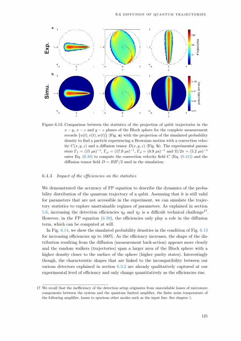
6.4 diffusion of quantum trajectories
a.
b.
Exp.
Simu.
Figure 6.13: Comparison between the statistics of the projection of qubit trajectories in the
x y, x z and y z planes of the Bloch sphere for the complete measurement
records u(t), v(t), w(t) (Fig. a) with the projection of the simulated probability
density to find a particle experiencing a Brownian motion with a convection veloc-
ity C(x, y, z) and a diffusion tensor D(x, y, z) (Fig. b). The experimental param-
eters Γ1 = (15 µs)1, Γϕ = (17.9 µs)1, Γd = (0.9 µs)1 and Ω/2 = (5.2 µs)1
enter Eq. (6.38) to compute the convection velocity field C (Eq. (6.41)) and the
diffusion tensor field D = BB†/2 used in the simulation.
6.4.3 Impact of the efficiencies on the statistics
We demonstrated the accuracy of FP equation to describe the dynamics of the proba-bility distribution of the quantum trajectory of a qubit. Assuming that it is still validfor parameters that are not accessible in the experiment, we can simulate the trajec-tory statistics to explore unattainable regimes of parameters. As explained in section5.6, increasing the detection efficiencies d and f is a difficult technical challenge17.However, in the FP equation (6.39), the efficiencies only play a role in the diffusionterm, which can be computed at will.
In Fig. 6.14, we show the simulated probability densities in the condition of Fig. 6.13for increasing efficiencies up to 100%. As the efficiency increases, the shape of the dis-tribution resulting from the diffusion (measurement back-action) appears more clearlyand the random walkers (trajectories) span a larger area of the Bloch sphere with ahigher density closer to the surface of the sphere (higher purity states). Interestinglythough, the characteristic shapes that are linked to the incompatibility between ourvarious detectors explained in section 6.3.2 are already qualitatively captured at ourexperimental level of efficiency and only change quantitatively as the efficiencies rise.
17 We recall that the inefficiency of the detection setup originates from unavoidable losses of microwavecomponents between the system and the quantum limited amplifier, the finite noise temperature ofthe following amplifier, losses to spurious other modes such as the input line. See chapter 5.
125

quantum trajectories
a.
b.
c.
d.
Figure 6.14: Projections of the simulated probability density on three planes of the Bloch sphere
in the configuration of Fig. 6.9. Fig. a is a simulation with the efficiencies f = 0.14
and d = 0.34 as in the experiment. We increase jointly the efficiencies f,d = 0.5
(Fig. b), f,d = 0.75 (Fig. c), and f,d = 1 (Fig. d). A clear broadening of the
distribution of states occurs for simulated higher detector efficiencies. The shape of
the distribution remains qualitatively the same except for unit efficiencies, which
is out of experimental reach.
126

6.4 diffusion of quantum trajectories
At unit efficiency, the quantum states is confined to a pure wavefunction diffusion onthe surface of the Bloch sphere. The characteristic shape of the projected distributionchanges in the last row of Fig. 6.14 but this situation is unreachable in practice18.
6.4.4 Convection velocity
We can gain insight into the transport phenomena of qubit states by analyzing theconvection velocity C. Using Eq. (6.41), the convection velocity reads
C(xt, yt, zt) =
0
@
Γ2xt Ωzt
Γ2yt
Γ1(1 + zt) + Ωxt
1
A+dΓd
2
0
@
xt(1 6z2t )
yt(1 6z2t )
6zt(1 z2t )
1
A+ fΓ1
0
@
xt(1 + zt 34(x2
t + y2t ))
yt(1 + zt 34(x2
t + y2t ))
14(1 + zt)(1 + zt 3(x2
t + y2t ))
1
A
(6.42)
where the inverse coherence time is Γ2 =Γ12 + Γd + Γ'.
The first term of Eq. (6.42) corresponds to the advection of the probability flow by thecircular motion induced by the Rabi torque and by the damping caused by decoherence.This advection term alone brings the qubit state along the average trajectory depictedin Fig. 6.13. The two other contributions emanate from the diffusive back-action ofthe measurements translated into the finite spread of the probability distribution. Theconvection of the probability flow takes place both by advection and by diffusion19.
a. b. c.
Figure 6.15: Cuts of the convection velocity field (6.42) in the x y (Fig. a), x z (Fig. b)
and y z (Fig. c) planes. The blue arrows correspond to C(xt, yt, zt)dt with
the parameters of Fig. 6.13 Γ1 = (15 µs)1, Γϕ = (17.9 µs)1, Γd = (0.9 µs)1,
Ω/2 = (5.2 µs)1 and dt = 100 ns. The solid black circle represents the pure
state of the plane that is also the rigid boundary condition for the FP equation.
In Fig. 6.15, we show cuts of the convection velocity field. In the plane hzi = 0
(Fig. a), the convection brings the qubit along the z-axis. Away from this plane, theconvection tends to bring quantum states to negative (resp. positive) x for hzi > 0
(resp. hzi < 0) planes (not represented on Fig. 6.15). Interestingly, a cut of the x z
18 At the time of writing this thesis, the highest total detection efficiency reported in the microwavedomain is 80% for a single dispersive channel [159].
19 This situation is reminiscent of convective heat transfer. For instance in fluid dynamics, the apparitionof Rayleigh–Bénard convection originates jointly from the diffusion of heat from the fluids to the platesand advection of heat in the fluid under the action of buoyancy and gravity.
127

quantum trajectories
plane (Fig. b) reveals two regions where the convection tends to vanish correspondingto the two maxima of the probability distribution of Fig. 6.13. The convection velocityin the x z plane is independent of the hyi value. Finally, Fig. c reveals that theconvection flow pushes the probability density toward the pointer states of the z
measurement (the poles) owing to its large measurement rate.
6.4.5 Diffusion tensor
In the Zeno regime, we showed that the general shape of the probability distribution canbe understood from an analysis of the convection velocity field. However, the diffusiontensor alone induces the non-deterministic behavior of the system. The diffusion doesnot depend on the applied drives, nor on unmonitored channels and thus exclusivelycharacterizes the measurement process. We can compute D = BB†/2 from Eq. (6.38).The diffusion can be decomposed into independent contributions20 corresponding tothe Wiener processes Wu, Wv and Ww
D(x, y, z) =1
2B(x, y, z)B(x, y, z)† = Du(x, y, z) +Dv(x, y, z) +Dw(x, y, z) (6.43)
where the independent contributions read
Du(x, y, z) =fΓ1
2
0
@
(1 + z x2)2 (1 + z x2)xy (1 + z)x(1 + z x2)
(1 + z x2)xy x2y2 x2y(1 + z)
x(1 + z)(1 + z x2) x2y(1 + z) x2(1 + z)2
1
A
Dv(x, y, z) =fΓ1
2
0
@
x2y2 (1 + z y2)xy xy2(1 + z)
(1 + z y2)xy (1 + z y2)2 (1 + z)y(1 + z y2)
xy2(1 + z) (1 + z)y(1 + z y2) y2(1 + z)2
1
A
Dw(x, y, z) = 2dΓd
0
@
x2z2 xyz2 (1 z2)xz
xyz2 y2z2 (1 z2)yz
(1 z2)xz (1 z2)yz (1 z2)2
1
A
In contrast to the convection velocity, the diffusion is given by a tensor field, whichcannot be easily represented inside the Bloch sphere. We further improve our under-standing of the diffusion by looking at two invariant quantities of the tensor, its deter-minant and trace.
6.4.6 Dimensionality of the diffusion
The determinant of the diffusion tensor tells whether, the diffusion occurs in all direc-tions or if it is singular and restricted a subspace of the Bloch sphere. If the randomwalk is confined in one direction (resp. two directions), the diffusion tensor will havetwo zero eigenvalues (resp. one zero eigenvalue) and a zero determinant. In this case,the quantum state can still diffuse in the complete Bloch ball if the vector fields of thestochastic Eq. (6.34) satisfy Hörmander’s condition [184]. Let us give a brief analysisto understand the dimensionality of diffusion in experimentally relevant situations.
20 The independence between the contributions to the diffusion tensor is a property of the stochastic
master equation (6.34). For a set of jump operators Lµ acting on a qubit, the diffusion tensor readsDi,j = 1
2
Pk Tr(Mk(ρ)σi)Tr(Mk(ρ)σj) where Mk(ρ) = Lkρ+ ρL†
k Tr(Lkρ+ ρL†k)ρ.
128

6.4 diffusion of quantum trajectories
In the case of a dispersive measurement alone, the only contribution to the diffusiontensor (6.43) is Dw, which has two zero eigenvalues. The diffusion is thus 1-dimensional.This is in agreement with the result of Sarlette and Rouchon [172] who showed that atevery time-step, the diffusion develops on an ellipse that shrinks toward the z axis of theBloch sphere according to Eq. (6.14). A similar result can be obtained when measuringthe orthogonal quadrature of the cavity field. The diffusion occurs on a deterministiccircle given by Eq. (6.18).
For an exclusive fluorescence measurement, the two contributions to the diffusiontensor (6.43) correspond to the Wiener processes Wu and Wv. The diffusion tensorD = Du+Dv has one zero eigenvalue revealing a 2-dimensional diffusion. The randomwalk takes place on the surface of a spheroid [23, 172] given by Eq. (6.25) that goesthrough the south pole of the Bloch sphere.
Recently, Hacohen-Gourgy et al. [49] were able to measure simultaneously two non-commuting observable of a qubit in a rotating frame namely the observables x and y.They observed an isotropic and persistent diffusion in x y plane when the strengthsof the two measurement are balanced. In their case, the diffusion tensor has one zeroeigenvalue revealing that they observed a 2-dimensional diffusion phenomenon in aplane.
By taking into account the outcomes of the two detectors in our experiment, thethree Wiener processes contribute to the diffusion (see Eq. (6.43)). The determinantreads
Det[D(x, y, z)] =dΓdfΓ1
8(1 + z)4
1 x2 y2 z2
2. (6.44)
The determinant annihilates on the surface of the Bloch sphere as it is not possible todiffuse in the direction orthogonal to the boundary. In the bulk of the Bloch ball, thedeterminant (6.44) takes finite values when the two channels are monitored df 6= 0.Our experiment is thus the first qubit experiment with a non zero determinant for thediffusion tensor revealing a genuine 3D diffusion in the volume of the Bloch ball.
6.4.7 Diffusivity
Instead of considering the diffusion along particular coordinates, we consider the ‘overall’diffusion. We express the average diffusivity as follows
d(x, y, z) = Tr[D(x, y, z)]. (6.45)
The diffusivity is a scalar field that represents the magnitude of the back-action at anypoint of the Bloch sphere regardless of the direction of the diffusion. This scalar field isinvariant under rotation around z. In Fig. 6.16, we represent cuts of the diffusivity inthe x z plane. We separate the different contributions coming from the monitoring ofthe cavity field (Fig. a), the monitoring of fluorescence (Fig. b) and the simultaneousmonitoring of both (Fig. c).
Whenever measuring continuously an observable (such as z) or an operator (such as), the quantum back-action stochastically kicks the quantum state to update it basedon the result of the measurement. However, the back-action vanishes when reaching the
129

quantum trajectories
a. b. c.
Figure 6.16: Magnitude of the average diffusivity given by Eq. (6.45) in a hyi = 0 slice of
the Bloch sphere for dispersive measurement (Fig. a), fluorescence measurement
(Fig. b) and both (Fig. c). In Fig. a, the diffusion is symmetric under z ! z. We
use the parameters of Fig. 6.13, Γ1 = (15 µs)1, Γd = (0.9 µs)1 and (f , d) =
(0.14, 0.34). Diffusion vanishes when the quantum state approaches one of the
pointer states of the z measurement (poles of the sphere). Monitoring energy
relaxation (Fig. b) leads to a maximal diffusivity at the north pole of the Bloch
sphere where the quantum state experiences the strongest measurement back-
action and minimal diffusivity in the ground state. The average magnitude of
the diffusion induced by this last measurement is much smaller than the one of
Fig. a because of the measurement rate asymmetryηfΓ1
ηdΓd' 0.025. The resulting
total diffusivity (Fig. c) only vanishes at the south pole of the Bloch sphere.
so-called pointer states of the measurement. In the case of a z measurement, the pointerstates are given by the poles of the Bloch sphere (Fig. 6.16 a). In between, the magnitudeof the coefficient diffusion is maximal near the equator so the qubit state ‘must’ jumpquickly from one region to the other in quantum trajectories. When monitoring , thesouth pole |gi of the Bloch sphere is the only pointer state (Fig. 6.16 b). When the qubitstate is close to the excited state |ei, the energy relaxation probability is maximal andthe back-action of the associated measurement chases the state away from the northpole. Hence, the total diffusivity (Fig. 6.16 c) only goes to zero in the ground state |gi.In the excited state, the diffusion is persistent even if the contribution of the dispersivemeasurement vanishes.
6.4.8 An Heisenberg-like inequality for pure states
We used throughout this thesis the concept of incompatible measurement to describethe quantum back-action of energy relaxation and dispersive measurement. We maywonder if there is an Heisenberg-like inequality for our system. The usual Heisenberg-Roberston uncertainty relation [185] states that the accuracy with which two Von Neu-mann measurements can be performed is limited by the restriction that the product ofthe uncertainties in the two measurements is at least of the order of the commutatorof the associated observables21.
21 In the case of the two conjugate variable X and P describing the free propagation of a particle, werecover the historical Heisenberg inequality σXσP ~/2.
130

6.4 diffusion of quantum trajectories
In the continuous measurement framework, the signature of the incompatibility ofthe measurement is encoded in a lower bound of the diffusion coefficients [186]. Weshow that the Heisenberg inequality finds its correspondence in a lower bound on thetotal diffusivity of pure states. From Eq. (6.37) we notice that Tr[BB†]dt = 2Tr[dd].We link the diffusivity to the incremental evolution of the density matrix22
d(x, y, z) =1
dtTr[dd]. (6.46)
For pure states, the quantity Tr[dd] is known to be related to the sum of the variancesof the measurements [49]. On the surface of the Bloch sphere, we obtain
d(x, y, z) = fΓ1 h(∆+)(∆)i+ dΓd h∆z2i (6.47)
where ∆A = AhAi. A complication arises from the fact that the monitored operator = (xiy)/2 is not hermitian nor skew-hermitian hence the apparition of + =
†.
However, we can develop
h(∆+)(∆)i =1
4
h∆x2i+ h∆y2i i h[x,y]i
. (6.48)
The two first terms are the variances associated to the measurement of the x and y
coordinates of the qubit, the last term shows how the hermitian and skew-hermitianparts interference of the jump operator associated to the energy relaxation channel. Inthe end, we obtain
d(x, y, z) =fΓ1
4h∆x2i+
fΓ1
4h∆y2i+ dΓd h∆z2i
fΓ1
4i h[x,y]i . (6.49)
The diffusivity is thus related to the sum of the variances associated to the measurementof every Pauli observable (plus the previously mentioned correction), and not to theirproduct like in the Heisenberg inequality. In the general case, for a pure state = | i h |and an arbitrary set of jump operators Lk, the diffusivity is linked to jump operatorsby the relation
Tr[dd] = 2X
k
k h |(∆L†k)(∆Lk)| i dt. (6.50)
Our task is thus to find a lower bound on h |(∆L†k)(∆Lk)| i = ||(∆Lk) | i ||2. Such a
lower bound is not unique. For incompatible observable, there always exists a non zerolower bound on the sum of incompatible observable [187]. This statement does not holdin general for operators. We can however give a lower bound on Eq. (6.50) using thegeometrical inequality
| h |L†| ?i |2 ||L | i ||2 (6.51)
valid for | ?i orthogonal to | i. In the end we obtain the following lower bound on thediffusivity
d(x, y, z) (1 + z)
fΓ1
2(1 + z) + dΓd(1 z)
. (6.52)
22 This identity is not specific to our system. It holds for any monitored open quantum system ruled bythe stochastic master equation (6.34).
131
quantum trajectories
In the excited state the diffusion never vanishes as it is lower bounded by the magni-tude of the back-action of energy relaxation 2fΓ1 (see Fig. 6.16). In the ground state,the lower bound vanishes as the back-action goes to zero. However, this is a specialcase for which the lower bound (6.52) is always saturated. The fact that the Heisenberginequality transforms into a lower bound on the diffusion is a signature of the enhance-ment of the diffusion due to the different measurements. Equilibrium points (pointerstates) correspond to where the diffusivity vanishes (see Fig. 6.16 or [49]). We talk abouta persistant diffusion around these points. The contributions of the measurements areindependent in Eq. (6.52). In the spirit of the Heisenberg inequality we ‘mix’ the twocontributions by application of the Cauchy-Schwarz inequality to Eq. (6.47)
d(x, y, z) p
fΓ1dΓd| h |∆+∆z| i |2 =pfΓ1dΓd
4(1 + z)2(x2 + y2) (6.53)
this last bound is similar to the one of [49] but it is weaker than Eq. (6.52) and itvanishes in the excited state.
6.5 conclusion
In this chapter we discussed
• the general framework for measurement back-action with the example of weakmeasurement of the dispersive and energy relaxation channels.
• the formalism of quantum trajectories leading to a stochastic diffusion in theBloch sphere.
• the shape of the trajectory statistics that contains the knowledge of differentobservers about a same quantum system.
• the Fokker-Planck equation revealing a 3-dimensional diffusion, which is charac-teristic of our incompatible measurements.
• an Heisenberg like inequality for continuous measurements of arbitrary operators.
Quantum trajectories have a bright future with numerous applications includingreal-time adaptative measurement [188], quantum parameter estimation with a neuralnetwork [189], the determination of the arrow of time from the irreversibility of quan-tum measurement [190], the observation of spikes in quantum trajectories [191, 192],investigation of chaos [193], the determination of quantum caustics [175, 25, 177] andapplications in single-shot quantum thermodynamics [194, 195, 196].
132

7POST - SELECTED QUANTUM TRAJECTORIES
Our everyday experience teaches us that the future is different from the past so wecan intuitively determine the direction of an arrow of time pointing towards the fu-ture. Time asymmetry arises in classical physics for irreversible evolution of either adissipative system or an out-of-equilibrium closed system with an internal dynamics.In the latter case, the irreversibility of the evolution is formalized by the second law ofthermodynamics, which proclaims that the entropy of an isolated system can never de-crease over time. In the absence of irreversibility, watching a ‘movie’ backwards showsan evolution consistent with the laws of physics.
In quantum mechanics, the Schrödinger equation for isolated system is time sym-metric as is its classical counterpart. In the 50s, von Neumann and Bohm [52, 53]suggested that the irreversible collapse of a wave packet of the state of a system underthe influence of measurement introduces a fundamental time asymmetry at the micro-scopic level. The measurement back-action was thus thought of as a time asymmetricelement in quantum theory. Nevertheless, the symmetry of the rules of quantum me-chanics is fully restored when specifying both the initial state and the final state ofa closed system. The equivalent role of preparation or pre-selection and post-selectionwas enlightened by Aharonov et al. in a seminal paper [54] and gave rise to the two-state vector formalism [197]. Aharonov et al. introduced a retrodiction estimation of aquantum state which was revisited in the case of open systems with the introduction ofan effect matrix [55, 56, 57, 58]. While the density matrix is the quantum state of thesystem conditioned on the past measurement records, the effect matrix is the quantumstate conditioned on the information available in the future. Taking into account theforward and backward estimation of the quantum state at the same time provides aso-called past quantum state that encapsulates all the information available from pastand future measurements.
In 1987, Aharonov noticed [59] that in the presence of both preparation and post-selection, the measured expectation values of the signal can spread outside of the nor-mal eigenvalue range. This anomalous values were called weak values [60]. Thus, on acarefully selected sub-ensemble of realizations of the experiment, the result of a weakmeasurement of a component of a qubit can in principle reach arbitrarily larges val-ues1. In this chapter, we present the results of an experiment illustrating this fact. Bycombining preparation and post-selection, the Bloch vector resulting from the directquantum tomography method exposed in chapter 3 exceeds the boundary of the unitsphere [61, 62, 63, 64].
Weak values were observed for the first time in 1991 [198] and have been shown to leadto a violation of Leggett-Garg inequality [61, 199, 200, 201] and thus to rule out macro-
1 In practice, the magnitude of the weak value is limited by the decoherence between preparation andpost-selection.
133

post-selected quantum trajectories
realistic physical theories2. Weak values are claimed to provide interesting features suchas noiseless amplification [202, 203, 60], a direct measurement of a wavefunction [204]or even to solve quantum ‘paradoxes’ [205]. These anomalous values seem to originatefrom a statistical effect arising from measurement back-action with preparation andpost-selection but this topic is the subject of considerable debates [206, 60, 207, 208,209, 210]. However there is no question that post-selecting realizations is well definedand that one needs the tools to predict the average outcome under post-selection. Thischapter intends to put the formalism to the test and understand its limitations.
Similarly to classical estimation theory, predictions on the outcome of a measurementat time t can be made by filtering given observations before and up to t, by retrodictiongiven the observations after t or by smoothing given observations before and after t.The smoothed estimate conditioned on the complete measurement record is obtainedby filtering and retro-filtering techniques [211, 57]. Using all the information extractedfrom the past and future measurements relative to the time at which an observableis estimated leads to an acausal smoothed estimation of the probability of outcomesassociated to this measurement [212].
First, let us introduce the past quantum state composed of the density matrix andthe effect matrix to describe pre-selected and post-selected trajectories [55, 56, 57, 58].Similarly to the density matrix, the effect matrix evolves according to a stochasticdifferential equation in the continuous times limit. This formalism is then related tothe weak values envisioned by Aharonov. Finally its operational meaning is investigatedby confrontation with our experimental results.
7.1 past quantum state
7.1.1 Prediction and retrodiction
This derivation is based on the work of Gammelmark et al. [58]. We introduce in thissection the effect matrix and the associated past quantum state. A quantum trajectoryis defined as iterated Kraus maps given by Eq. (6.31)
tn+1 =Ky(tn)(tn)
Tr[Ky(tn)(tn)]=
Ky(tn) ... Ky(t0)(0)
Tr[Ky(tn) ... Ky(t0)(0)](7.1)
where we define the discrete times tn = ndt between each time step of the trajectoryfor 0 n N and ytn are the vectors of the measurement records at each time.For a system with a set of jump operators Lµ, the partial Kraus map giving theincremental evolution during dt is given by Eq. (6.28)
8
>>>>><
>>>>>:
Ky(t)(t) = My(t)tM†y(t) +
X
µ 6=0
(1 µ)dtLµtL†µ
with My(t) = 1
0
@i
~H +
X
µ 6=0
L†µLµ/2
1
A dt+X
µ 6=0
pµLµyµ(t)dt
(7.2)
2 under the assumption that the detector does not disturb the system in a classical sense.
134
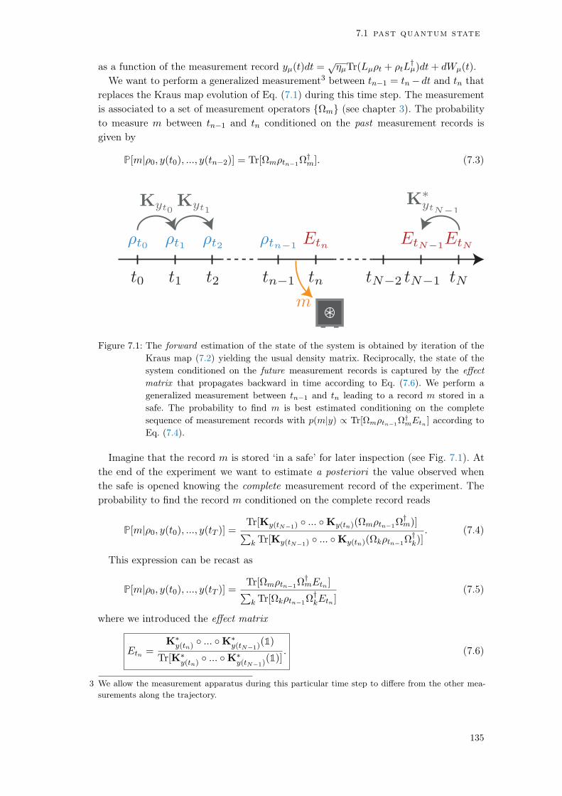
7.1 past quantum state
as a function of the measurement record yµ(t)dt =pµTr(Lµt + tL
†µ)dt+ dWµ(t).
We want to perform a generalized measurement3 between tn1 = tn dt and tn thatreplaces the Kraus map evolution of Eq. (7.1) during this time step. The measurementis associated to a set of measurement operators Ωm (see chapter 3). The probabilityto measure m between tn1 and tn conditioned on the past measurement records isgiven by
P[m|0, y(t0), ..., y(tn2)] = Tr[Ωmtn1Ω†m]. (7.3)
Figure 7.1: The forward estimation of the state of the system is obtained by iteration of the
Kraus map (7.2) yielding the usual density matrix. Reciprocally, the state of the
system conditioned on the future measurement records is captured by the effect
matrix that propagates backward in time according to Eq. (7.6). We perform a
generalized measurement between tn1 and tn leading to a record m stored in a
safe. The probability to find m is best estimated conditioning on the complete
sequence of measurement records with p(m|y) / Tr[Ωmtn−1Ω
†mEtn ] according to
Eq. (7.4).
Imagine that the record m is stored ‘in a safe’ for later inspection (see Fig. 7.1). Atthe end of the experiment we want to estimate a posteriori the value observed whenthe safe is opened knowing the complete measurement record of the experiment. Theprobability to find the record m conditioned on the complete record reads
P[m|0, y(t0), ..., y(tT )] =Tr[Ky(tN1) ... Ky(tn)(Ωmtn1Ω
†m)]
P
k Tr[Ky(tN1) ... Ky(tn)(Ωktn1Ω†k)]
. (7.4)
This expression can be recast as
P[m|0, y(t0), ..., y(tT )] =Tr[Ωmtn1Ω
†mEtn ]
P
k Tr[Ωktn1Ω†kEtn ]
(7.5)
where we introduced the effect matrix
Etn =K
y(tn)
... Ky(tN1)
(1)
Tr[Ky(tn)
... Ky(tN1)
(1)]. (7.6)
3 We allow the measurement apparatus during this particular time step to differe from the other mea-surements along the trajectory.
135
post-selected quantum trajectories
The adjoint4 of the Kraus map is Ky(t)(E) = M †
y(t)EMy(t)+P
µ(1µ)dtL†µELµ. The
effect matrix is an estimation of the state of the qubit conditioned on the informationavailable from the ‘future’5 measurement records of the trajectory. This hermitian ma-trix evolves backward in time by application of the conjugated Kraus maps accordingto the retrodiction formula
Etn =K
y(tn)
(Etn+1)
Tr[Ky(tn)
(Etn+1)]. (7.7)
The time symmetry of the formalism is restored by specifying the final state of theevolution EtN along with the initial condition t0 . Note that in the absence of post-selection after time tN , EtN = 1
2 . In contrast, in the absence of preparation, t0 is in itsequilibrium thermal state.
The pair of matrices Ξtn = (tn1 , Etn) is called the past quantum state in the for-malism of Gammelmark et al. [58]. It contains all the available information to make apredictions about the outcome of a measurement occurring between tn1 and tn thanksto Eq. (7.5). The introduction of an initial (preparation) and final (post-selection) se-lection procedures makes our formalism perfectly time symmetric in the absence ofdissipation.
7.1.2 Continuous time dynamics
In the continuous time limit, the Kraus map defined by Eq. (7.2) reads
Ky(t)(Et+dt) = Et+dt +
i
~[H,Et+dt]dt+
X
µ
dt(L†µEt+dtLµ L†
µLµ
2Et+dt Et+dt
L†µLµ
2)
+X
µ
pµ(L
†µEt+dt + Et+dtLµ)yµ(t)dt.
(7.8)
And since Tr(Ky(t)(Et+dt)) = 1+
P
µpµTr(L
†µEt+dt +Et+dtLµ)yµ(t)dt. The normali-
sation factor can be approximated at order dt by
1
Tr(Ky(t)(Et+dt))
= 1X
µ
pµTr(L
†µEt+dt + Et+dtLµ)yµ(t)dt
+X
µ
µTr(L†µEt+dt + Et+dtLµ)
2dt.(7.9)
At first order in dt, the evolution of the effect matrix is ruled by a stochastic masterequation6
dEt = i
~[H,Et]dt
mX
i=1
Di (Et)dt
mX
i=1
piMi(Et)
yµ(t)dt Tr(L†µEt EtLµ)dt
4 The adjoint of K is defined by Tr[AK(B)] = Tr[K(A)B] for any hermitian operators A,B.5 The notion of future and past is referred to the time tn, at which the record of the generalized
measurement is stored in the safe.6 In [58] they use the backward time definition for the following equation (7.10). We use the forward
time t > 0 instead.
136

7.1 past quantum state
(7.10)
where the adjoint of Lindblad operator reads Di (Et) = L†
iEtLi (L†iLiEtEtL
†iLi)/2,
the innovation super-operator is Mi(Et) = L†iEt + EtLi Tr(L†
iEt + EtLi)Et.
preparation post-selection
prediction retrodiction
Figure 7.2: The state of the system can be predicted conditioned on past measurement records
using the density matrix t provided by the stochastic master equation (see
Eq. (6.34) in chapter 6). Conversely the state of the system can be rectrodicted,
a posteriori, conditioned on the future measurement records by unravelling the ef-
fect matrix Et with Eq. (7.10). The past quantum state (t, Et) uses the complete
measurement records to give an estimate of the distribution of any measurement
performed on the system at time t according to Eq. (7.12).
In the case of unread measurements (i = 0), we obtain the equivalent of the Lindbladequation for the effect matrix with an adjoint Lindblad super-operator
dEt = i
~[H,Et]dt
mX
i=1
Di (Et)dt. (7.11)
When pre and post-selecting the evolution, we average a selected ensemble of realiza-tions of the experiments. The recorded signal is thus impacted. On a large number ofrealizations, the experimentalist acquires a mean smoothed measurement record ySµ (t)
associated to a jump operator Lµ with an efficiency µ instead of the mean of the usualrecord yµ(t). The mean smoothed measurement records in presence of preparation andpost-selection reads [55, 58, 85]
ySµ (t)dt =Tr[Et
pµ(Lµt + tL
†µ)]
Tr[Ett]dt = 2Re[
Tr[pµtEtLµ]
Tr[tEt]] = 2
pRe[hLiw]
(7.12)
where h.iw denotes the expectation value conditioned on the full measurement record.The quantity tEt
Tr[tEt]plays the analog of a density matrix even if it does not define a
quantum state7. Note that it is possible to defined a quantum smoothed state using thecomplete measurement record [213] but we will not need it in the rest of the manuscript.
7 The matrix ρtEt
Tr[ρtEt]is not a density operator because it is not Hermitian or (even if symmetrized)
positive semi-definite.
137

post-selected quantum trajectories
An important feature of the formalism is that Eq. (7.12) is proportional to the realpart of the weak value of the jump operator. The generalized weak value of an operatorA is defined as follows8 [55]
hAiw =Tr[AtEt]
Tr[tEt]. (7.13)
The magnitude of the weak value given by Eq. (7.13) can in principle diverge as thedenominator can be very small and even reaches zero when the past (density matrix)and future (effect matrix) quantum states are orthogonal. The conditioned measuredaverages can lie outside of the unconditioned range. However as we will see, both thedensity matrix and the effect matrix evolve into a statistical mixture between pre andpost selection owing to decoherence preventing a perfect orthogonality of the two states.Therefore, decoherence sets an upper bound on the measured weak value.
This formalism is an extension of chapter 6. Indeed, we can recover the usual casewithout post-selection by setting E = 1/2 in Eq. (7.13) but we can also use exclusivelythe backward estimate by setting = 1/2. Now that we introduced the past quantumstate that uses the whole measurement records, let us confront it with experimentalresults with preparation and post-selection.
7.2 pre and post-selected trajectories
7.2.1 Time symmetric Rabi evolution
In the experiment, our qubit is driven with an Hamiltonian H = ~Ω
2 y. The averageevolution of the density matrix is given by the Lindblad equation (see section 3.4)
dtdt
= i[Ω
2y, t] +
Γd + Γ'
2D[z](t) + Γ1D[](t) (7.14)
where Γ1 is the inverse lifetime of the qubit, Γd is the measurement induced dephasingrate and Γ' is the pure dephasing rate. The Lindblad super-operator is D[L]() =
LL† 12(L
†L + L†L). The qubit is prepared at time t = 0 in a state 0 that givesthe initial condition of Eq. (7.14). Note that we neglected qubit excitation in Eq. (7.14)since the excitation probability of the qubit in thermal equilibrium was measured tobe lower than 2%.
The unmonitored evolution of the effect matrix E evolves backward in time accordingto Eq. (7.11). In our experiments, it reads (in the forward sense)
dEt
dt= i[
Ω
2y, Et]
Γd + Γ'
2D[z](Et) Γ1D
[](Et) (7.15)
where Di (Et) = L†
iEtLi (L†iLiEt EtL
†iLi)/2.
8 This is a generalization to mixed states of the historical weak value hAiw = hψf |A|ψii / hψf |ψii envi-sioned by Aharonov [59].
138

7.2 pre and post-selected trajectories
a.
-1.0-0.50.0
0.5
1.0
0.0
-1.0-0.5
0.5
1.0
0 5 10 15 20 25 30
-1.0-0.50.0
0.5
1.0
0 5 10 15 20 25 300 5 10 15 20 25 30
b. c. d.
e. f. g.
h. i. j.
Figure 7.3: a. Pulse sequence and measurement setup. The qubit is prepared in |gi or in a
statistical mixture of |gi and |ei. During the experiment, the qubit is driven by a
continuous tone at fq. The state of the cavity is concurrently probed by sending
a tone at fc leading to the continuous measurement records w(t) in Eq. (7.16).
The spontaneous emission of the qubit is recorded at the same time yielding to
the records u and v in (7.16). At the end of the experiment we perform a pro-
jective measurement of the spin along a given axis of the bloch sphere. In this
experiment, we pre and post-select only on |gi. b. e. h. Pre-selected trajectory.
The solid line is the solution of the Lindblad equation (7.14) with the parameters
Γ1 = (10.4 µs)1, Γϕ + Γd = (22 µs)1, Ω/2 = (875 ns)1 while the dots are the
measured records u(t), v(t) w(t), here raw averaged on the selected ensemble out
of the 36 million realizations of the experiment. In this case 2Re[hi] = hxiρ and
2Im[hi] = hyiρ corresponds to the Bloch coordinates. d. g. j. Post-selected
trajectory (without pre-selection meaning 0 = 1/2). The lines are the solutions
of the equation (7.15) with the above-mentioned parameters. The average mea-
surements records (dots) are superimposed. In this case, 2Re[hi] = hxiE and
2Im[hi] = hyiE are the Bloch coordinates of the retrodicted quantum state. c.
f. i. Pre and post-selected trajectory. The solid lines are the prediction of Eq. (7.16)
where the density matrix is calculated from the Lindblad equation (7.14) and the
effect matrix is obtained from Eq. (7.15) with the same parameters as in the other
plots. We observe a good agreement between these smoothed measurement records
and the experimental records (dots) raw averaged on the pre and post-selected
ensembles of trajectories.
139
post-selected quantum trajectories
The system is post-selected at time T in a state ET that defines the final conditionof Eq. (7.15). Note that Eq. (7.15) is not the exact time symmetric9 of Eq. (7.14).Although, the decoherence term is symmetric in time D[z](E) = D[z](E), the energydissipation for the effect is D[](E) 6= D[](E). This last term vanishes when E =
1/2 in contrast to the dissipation term of Eq. (7.14) D[]() which cancels for =
|gi hg| [85]. In this section, the Rabi rate Ω of the Hamiltonian evolution dominates thedecoherence rates of the system. The asymmetry induced by dissipation is thereforenot straightforwardly observable.
We can use both the density matrix and the effect matrix to predict the measurementrecords averaged on a pre and post-selected ensemble of trajectories given in Eq. (7.12)
8
>><
>>:
uS(t)dt =p
2fΓ1Re[hiw]dtvS(t)dt =
p
2fΓ1Im[hiw]dtwS(t)dt =
p
2dΓdRe[hziw]dt(7.16)
where the weak value is defined as hAiw = Tr[AE]/Tr[E] (see Eq. (7.13)).A striking feature of the weak values in Eq. (7.16) is that the real and imaginary part
functions do not ‘commute’ with the average h.iw. For instance the real part of hiw isnot hxiw /2 = hRe[]iw because E is not Hermitian. Let us denote p = E/Tr[E],we can write
Re[hiw] =1
2Re[Tr[p(x iy)]]
=1
2Tr[Re[p]x Im[p]y]
6= 1
2Re[Tr[px]]
. (7.17)
In our detection setup (see Fig. 7.3 a), monitoring the fluorescence emitted by a qubitwill no longer be equivalent to obtaining information on x = 2Re[] on one quadra-ture and y = 2Im[] along the other quadrature as it was the case in section 3.3. Apre and post-selected homodyne detection of an electromagnetic wavepacket can thusaccess the properties of both the real and the imaginary part of the field. This fact isthe basis of wavefunction tomography protocols based on weak values [204, 60]. Thepre-selected (resp. post-selected) measurement records can be recovered from Eq. (7.16)by setting E = 1/2 (resp. = 1/2). In this case, u, v and w are proportional to theexpectation values of x, y and z for the quantum state (forward estimation) or E(backward estimation).
Pre-selection (resp. post-selection) is experimentally achieved by performing a projec-tive measurement (see chapter 3) at the beginning (resp. at the end) of the experimentalong a given axis of the Bloch sphere. Trajectories are averaged conditionally on thefinal and initial projective measurement outcome revealing the smoothed measurementrecords (7.16).
In Fig. 7.3, we perform a pre and/or post-selection of a 30 µs long Rabi oscillation.In the pre-selected traces (Fig. 7.3 b e h), the qubit is initialized in |gi and then
9 The two equations are not time symmetric as soon as one of the jump operators is not Hermitian norskew-Hermitian.
140

7.2 pre and post-selected trajectories
experiences usual Rabi oscillations in the presence of weak decoherence. The Blochvector oscillates around the y axis in the xz plane and converges toward the center ofthe Bloch sphere. In the post-selected case (Fig. 7.3 d g j), the qubit state starts10 in1/2 and then experiences time reversed Rabi oscillations before reaching its final stateET = |gi hg|. Finally, when the trajectories are both pre and post-selectioned (Fig. 7.3c f i), the amplitude of the oscillation starts to decrease because of the Lindbladsuper-operator in Eq. (7.14) before increasing again under the action of the adjointLindblad operator in Eq. (7.15). The time t = T/2 defines a plane of symmetry forthe trajectory enlightening the time symmetry of the past quantum state formalismwhen the dynamics is dominated by a fast Hamiltonian evolution. In the middle ofthis pre and post-selected average trace, the amplitude of the oscillation (Fig. 7.3 c
i) is greater than the one for the forward prediction (Fig. 7.3 b h) or the backwardretrodiction (Fig. 7.3 d j). We will demonstrate in the next section that this abnormallyhigh amplitude can even exceed ±1.
7.2.2 "Anomalous" weak values
The denominator of the weak value (7.13) is just the probability for the sequence offuture measurement results
Tr[tEt] = P[yt<<T |t]/Tr[Ky(tn)
... Ky(tN1)
(EtN )]. (7.18)
If the future measurement records y>t are very ‘unlikely’ given the density matrixt at time t, the weak value at this time will be ‘large’ because of the near orthogonalityof t and Et. They can even surpass the extremal eigenvalues of the measured operatorleading to the ‘anomalous’ weak values predicted by Aharonov et al. [59]. The obser-vation of these anomalous values has been claimed to contradict macro-realism whenusing a non-invasive detector11 equivalently to the violation of Leggett-Garg inequality[61, 199, 200, 201]. At a given time t orthogonality of the states t and Et is limitedby the Lindblad terms in Eq. (7.14) and Eq. (7.15) that reduces the purity12 of thestates for lengthy evolution. We thus reduce the duration of the experiment from 30 µs
(Fig. 7.3) to 1.7 µs (Fig. 7.4) to increase the combined effect of pre and post-selectionby reducing the effect of decoherence.
In Fig. 7.4, we pre and post-select a trajectory on a very unlikely future outcome(Fig. 7.4 a). We observe again a good agreement between the calculated smoothedrecords (7.16) and the experimental measurement records averaged conditionally onthe outcomes of pre and post-selection (Fig. 7.4 b d). We emphasize that the measure-ment records do not correspond to the pre and post-selected expectation of the Pauliobservable (see Eq. 7.17) by representing Re[hxiw] as a solid line in Fig. 7.4 b. In con-trast to Fig. 7.3, the measured signal reaches values beyond ±1 that are not permittedfor only pre or post-selected averages. This is an illustration of the amplifying property
10 We artificially prepare an equal statistical mixture of |gi and |ei by averaging with the appropriateweighting coefficients trajectories pre-selected in |gi and in |ei.
11 Our detection setup can be considered as non-invasive as cryogenic circulator isolate the system fromthe detection setup.
12 Only pure states can be perfectly orthogonal in the Bloch sphere.
141

post-selected quantum trajectories
of weak values [202, 203, 60]. In this regions, the sensitivity of our detection on smallvariation of the parameters13 of the system is increased as the weak values are inverselyproportional to the almost vanishing scalar product between t and Et. This feature iseven more salient when the conditioned records are represented in 3D. As explained inchapter 3, raw averaging the unconditioned measurement records amounts to directlyimaging the Bloch vector. When pre and post-selected, the imaged vector norm cannow exceed 1 and thus explore the outside of the unit sphere14 (see Fig. 7.5 a).
0.0 0.5 1.0 1.5-3-2-10
1
2
3
0.0 0.5 1.0 1.5
-3-2-101
2
3
0.0 0.5 1.0 1.5-3-2-10
1
2
3
a. b.
c.d.
Figure 7.4: a. We perform a pre-selection in the ground state 0 = |gi hg| and a post-selection
in an arbitrarily chosen state ET such that (Tr[xET ],Tr[yET ],Tr[zET ]) =
(sin(), 0, cos()) where = 238/180. The pre (dark blue), post (dark yel-
low), pre and post (purple) selected trace are observed through the measurement
records 2Re[hi] (Fig. b), 2Im[hi] (Fig. c) and Re[hzi] (Fig. d). Similarly
to Fig. 7.3, the solid lines are predicted from the smoothed measurement record
(7.16) calculated from the density matrix and effect matrix obtained from Eq. (7.14)
and Eq. (7.15) with the parameters Γ1 = (11 µs)1, Γϕ + Γd = (12.3 µs)1 and
Ω/2 = (850 ns)1. Both Fig. b and d show values that exceed the range of pos-
sible unconditional average values delimited by the green dashed lines. The vector
obtained by raw averaging of the three measurement records lies outside of the
sphere of radius 1. We additionally represent Re[hxiw] as a black line in Fig. b
illustrating the stark difference between this quantity and the measured record
2Re[hiw] = Re[hx iyiw] with pre and post-selection. Note that in the exper-
iment, the pre and post-selected trace exhibit an offset in the v(t) record (Fig. c)
that is not predicted by theory.
13 For instance, a small change in the Rabi rate or in the pre and post-selection fidelities changes dra-matically the amplitude of the weak value.
14 This does not contradict the quantum theory as the pre and post-conditioned imaged vector does notcorrespond to the Bloch vector of a quantum state.
142
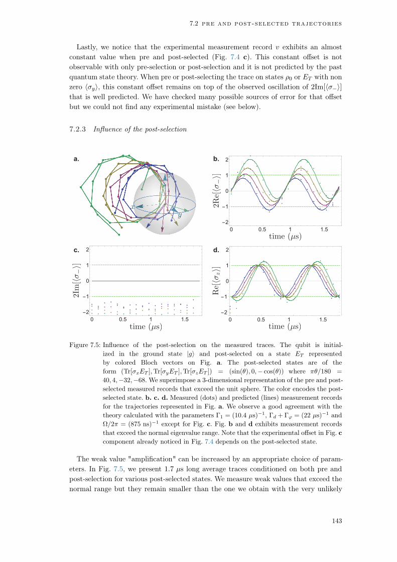
7.2 pre and post-selected trajectories
Lastly, we notice that the experimental measurement record v exhibits an almostconstant value when pre and post-selected (Fig. 7.4 c). This constant offset is notobservable with only pre-selection or post-selection and it is not predicted by the pastquantum state theory. When pre or post-selecting the trace on states 0 or ET with nonzero hyi, this constant offset remains on top of the observed oscillation of 2Im[hi]that is well predicted. We have checked many possible sources of error for that offsetbut we could not find any experimental mistake (see below).
7.2.3 Influence of the post-selection
a. b.
c. d.
0 0.5 1 1.5
-2-10
1
2
0 0.5 1 1.5
-2-10
1
2
0 0.5 1 1.5
-2-10
1
2
Figure 7.5: Influence of the post-selection on the measured traces. The qubit is initial-
ized in the ground state |gi and post-selected on a state ET represented
by colored Bloch vectors on Fig. a. The post-selected states are of the
form (Tr[xET ],Tr[yET ],Tr[zET ]) = (sin(), 0, cos()) where /180 =
40, 4,32,68. We superimpose a 3-dimensional representation of the pre and post-
selected measured records that exceed the unit sphere. The color encodes the post-
selected state. b. c. d. Measured (dots) and predicted (lines) measurement records
for the trajectories represented in Fig. a. We observe a good agreement with the
theory calculated with the parameters Γ1 = (10.4 µs)1, Γd + Γϕ = (22 µs)1 and
Ω/2 = (875 ns)1 except for Fig. c. Fig. b and d exhibits measurement records
that exceed the normal eigenvalue range. Note that the experimental offset in Fig. c
component already noticed in Fig. 7.4 depends on the post-selected state.
The weak value "amplification" can be increased by an appropriate choice of param-eters. In Fig. 7.5, we present 1.7 µs long average traces conditioned on both pre andpost-selection for various post-selected states. We measure weak values that exceed thenormal range but they remain smaller than the one we obtain with the very unlikely
143
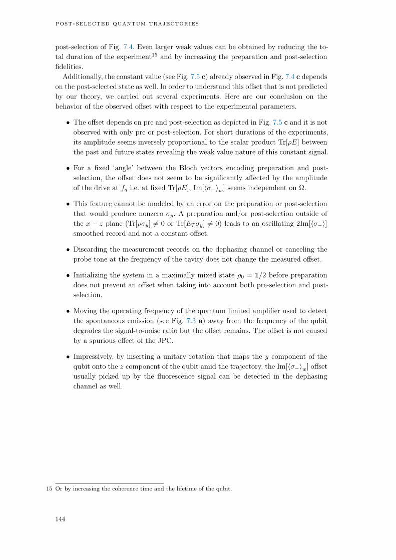
post-selected quantum trajectories
post-selection of Fig. 7.4. Even larger weak values can be obtained by reducing the to-tal duration of the experiment15 and by increasing the preparation and post-selectionfidelities.
Additionally, the constant value (see Fig. 7.5 c) already observed in Fig. 7.4 c dependson the post-selected state as well. In order to understand this offset that is not predictedby our theory, we carried out several experiments. Here are our conclusion on thebehavior of the observed offset with respect to the experimental parameters.
• The offset depends on pre and post-selection as depicted in Fig. 7.5 c and it is notobserved with only pre or post-selection. For short durations of the experiments,its amplitude seems inversely proportional to the scalar product Tr[E] betweenthe past and future states revealing the weak value nature of this constant signal.
• For a fixed ‘angle’ between the Bloch vectors encoding preparation and post-selection, the offset does not seem to be significantly affected by the amplitudeof the drive at fq i.e. at fixed Tr[E], Im[hiw] seems independent on Ω.
• This feature cannot be modeled by an error on the preparation or post-selectionthat would produce nonzero y. A preparation and/or post-selection outside ofthe x z plane (Tr[y] 6= 0 or Tr[ETy] 6= 0) leads to an oscillating 2Im[hi]smoothed record and not a constant offset.
• Discarding the measurement records on the dephasing channel or canceling theprobe tone at the frequency of the cavity does not change the measured offset.
• Initializing the system in a maximally mixed state 0 = 1/2 before preparationdoes not prevent an offset when taking into account both pre-selection and post-selection.
• Moving the operating frequency of the quantum limited amplifier used to detectthe spontaneous emission (see Fig. 7.3 a) away from the frequency of the qubitdegrades the signal-to-noise ratio but the offset remains. The offset is not causedby a spurious effect of the JPC.
• Impressively, by inserting a unitary rotation that maps the y component of thequbit onto the z component of the qubit amid the trajectory, the Im[hiw] offsetusually picked up by the fluorescence signal can be detected in the dephasingchannel as well.
15 Or by increasing the coherence time and the lifetime of the qubit.
144

7.3 conclusion
7.3 conclusion
In this chapter, we demonstrated
• that prediction and retrodiction of the evolution of a qubit that is prepared andpost-selected in chosen states using the past quantum state formalism describeexperimentally relevant situation.
• that our full quantum tomography method can lie outside of the Bloch sphere bycombining preparation and post-selection. This is an observation of a weak value.
• the apparition of an a constant signal on the imaginary quadrature of the fluo-rescence signal when both pre and post-selecting. That offset is not predicted bytheory and it requires further investigation.
Weak values are at the heart of colorful theoretical debate as they are often mis-understood [60]. A way to circumvent this difficulty is to define a smoothed quantumstate [213, 214, 215] using the complete available knowledge a posteriori. This smoothedquantum state belongs to the operator space as opposed to the past quantum ‘state’Ξt = (t, Et) introduced by Gammelmark et al. [58]. Moreover, such a smoothed esti-mate made from incomplete observations are predicted to outperform estimates madeusing full knowledge of the causal quantum state [214]. This might be observed by un-raveling quantum trajectories, not only for the density matrix as in chapter 6, but alsofor the effect matrix [63], for both [64] and for the smoothed quantum state. Manifes-tations of the interference between initial and final states can be revealed through thestatistics of pre and post-selected measurement records such as peaks or dips at half-quantized value of the measurement outputs [216]. Finally, the time asymmetry inducedby dissipation could be studied by comparing the statistics of forward and backwardquantum trajectories. The arrow of time could emerge by comparing the likelihood ofthe forward and backward propagation hypotheses [190].
145


Part III
APPENDIX


ATRANSMON COUPLED TO A TRANSMISS ION L INE
This appendix follows a lecture given by Pierre Rouchon at the CIRM school : Modelingand Control of Open Quantum Systems in April 2018. It gives a prototypical derivationof the dynamics of an open quantum system: a transmon qubit coupled to a trans-mission line modeled as a collection of harmonic oscillators. Special care is given tothe treatment of the Markov approximation to obtain the Langevin equation. We alsobring to light the fact that the non linearity of the junction is distributed among all theelements of the circuit including the coupling capacitance to the transmission line [82].This problem is crucial in this thesis because it takes on the problem of relaxation andmeasurement of an atom by spontaneous emission, which is central for the heterodynemeasurement of the energy relaxation of a transmon qubit in our experiments. We showthat extra higher order terms appear in the derivation of the input-output relation ofan anharmonic oscillator such as the transmon. However, the additional terms give riseto a negligible non linear correction to the dissipation. This effect exactly vanishes fora qubit but it might be of importance for high impedance circuits.
a.1 classical equation of motions
We start by introducing the classical equations of motion of the system depicted inFig (A.1). In this description the transmission line was replaced by an infinite collectionof discrete l∆, c∆ modes at positions x = 0,∆, 2∆, .... We also assume that the couplingcapacitance Cl satisfies Cl C. Together with the Ohmic modeling of the semi-infinitetransmission line, this assumption plays the role of the so-called Markov approximation.
a.1.1 Dynamics of the system
The Lagrangian of the system reads
L =C
2Φ2 +
Cl
2(Φ0 Φ)2 +
X
r0
c∆
2Φ2r + EJ cos(Φ/'0)
X
r0
(Φr+1 Φr)2
2l∆ (A.1)
where the reduced flux quantum is '0 = ~/2e. We have the associated conjugatedvariables
8
>>>>>><
>>>>>>:
Q =@L
@Φ= CΦ+ Cl(Φ Φ0)
q0 =@L
@Φ0
= Cl(Φ0 Φ) + c∆Φ0
qr =@L
@Φr
= c∆Φr
. (A.2)
149

transmon coupled to a transmission line
a. b.
Figure A.1: a. A transmon is capacitively coupled to a transmission line by a capacitor Cl. The
transmon is composed of a Josephson junction of Josephson energy EJ shunted by
a large capacitor C. We neglect the intrinsic capacitance of the junction. We assume
that Cl C to ensure that the system can be treated as a well defined system
coupled to a zero memory bath. b. We decompose the electromagnetic modes of
the transmission line in discrete modes spaced by a distance ∆. We denote by l
and c the inductance and capacitance per unit length of the transmission line. Φ
is the voltage across the junction and Φr is the voltage across the rth capacitance
of the transmission line.
A Legendre transform of the Lagrangian (A.1) gives the Hamiltonian
H(Φ, Q, Φr, qr) =@L
@ΦΦ+
X
r0
@L
@Φr
Φr L
=(Q+ q0)
2
2C+
q202Cl
+(Φ1 Φ0)
2
2Cl EJ cos(Φ/'0)
+X
r1
q2r2c∆
+(Φr+1 Φr)
2
2l∆.
(A.3)
We can then write Hamilton’s equations of motion as8
>>>>>>>>>>>>>>>>>><
>>>>>>>>>>>>>>>>>>:
dΦ
dt=
Q+ q0C
dQ
dt= EJ
'0sin(Φ/'0)
dΦ0
dt=
q0Cl
+Q+ q0
Cdq0dt
=Φ1 Φ0
l∆dΦr
dt=
qrc∆
dqrdt
=Φr+1 2Φr + Φr1
l∆
. (A.4)
By combining two equations of (A.4), we have
d2Φr
dt2=
Φr+1 2Φr + Φr+1
lc∆2. (A.5)
150

A.1 classical equation of motions
In the continuous limit (∆ 1), we can write the flux as a function of positionΦr(t) = Φ(t, r∆) where the function Φ(t, x) satisfies Dalembert’s equation with velocity1/
plc
@2Φ
@t2=
1
lc
@2Φ
@x2. (A.6)
The flux along the transmission line can be decomposed into left and right propagat-ing plane waves Φ(t, x) = Φin(t +
plcx) + Φout(t
plcx) allowing us to recover the
usual input-output relation at x = 0
Φ(t, 0) = Φin(t) + Φout(t) = Φ0(t). (A.7)
The derivative of the input-output relation (A.7) reads
Φin(t) + Φout(t) = Φ0(t) = q0
1
C+
1
Cl
+Q
C. (A.8)
We can approximate the derivative of the charge at position x = 0 by
dq0dt
=Φ1 Φ0
l∆=
Φin(t+plc∆) + Φout(t
plc∆) (Φin(t) Φout(t))
l∆
'r
c
l(Φin(t) Φoutt))
. (A.9)
We end up with the following system of coupled equations8
>>>>>>>>>>><
>>>>>>>>>>>:
Φout(t) = Φin(t) +Q+ q0
C+
q0Cl
dq0dt
=
rc
l
2Φin(t)Q+ q0
C+
q0Cl
dΦ
dt=
Q+ q0C
dQ
dt= EJ
'0sin(Φ)
(A.10)
Let us introduce the small parameter = Cl
C+Cl. We assumed in the situation depicted
on Fig. A.1 that was very small with the so-called Markov approximation. We willexpand the solutions of the problem of Fig. A.1 up to the first non trivial order in .From (A.10), the method of ‘variation of constants’ gives
d(q0(t)ezt/C)
dt= z
2Φin(t)Q(t)
C
ezt/C (A.11)
where z =q
lc is the impedance of the transmission line. An integration between 0 and
+1 leads to
q0(t) = z
Z +1
0dt0
2Φin(t0) Q(t0)
C
ez(tt0)/C
=
Z +1
0e(2CΦin(t )Q(t ))d
(A.12)
where = Cz.
151
transmon coupled to a transmission line
a.1.2 Asymptotic expansion in
first order in
Let us expand Eq. (A.12) with respect to . At first order,
q0(t) = (2CΦin(t)Q(t)). (A.13)
By using this expression with Eq. (A.10), we get
Φout = Φin +q0C
(1 +O()) +Q
C(A.14)
which leads to the trivial input-output relation
Φout(t) = Φin(t). (A.15)
There is no information in the reflected signal at first order in in (A.12), we must goto the second order.
second order in
We can expand Q and Φ in with respect to
Q(t ) = Q(t) Q(t) = Q(t) +EJ
'0sin(Φ(t)/'0 )
Φ in (t) 'Z +1
0e
Φ in (t )d
. (A.16)
The dynamics of the system is governed by8
>><
>>:
dΦ
dt=
(1 )
CQ(t) +
2Φ in (t) EJ
'0sin(Φ(t))
dQ
dt= EJ
'0sin(Φ/'0 )
(A.17)
In the end, the input-output relation now reads
Φout (t) = Φ in (t) EJ
'0Csin(Φ/'0 ). (A.18)
We clearly see that this input-output is non linear and it gives us information on sin(Φ).We will now transpose this equations in the quantum world to recover the input-outputrelation used in our system and study the impact of the non-linearity of this relation.
a.2 quantum description
Following [217], the incoming modes propagating along the transmission line can bedecomposed as
' in (t, x) =1
2
r
1
l
c
1/4 Z 1
0
p!d!
a in (!)ei!(t+
plcx) + h.c.
. (A.19)
152

A.2 quantum description
with the commutation relation [a in (!), a†in (!
0 )] = (! ! 0 ). A difficulty arises inthis description because we cannot simply define the temporal mode operators of thetransmission line to be
b in (t) =1
2
r
1
l
c
1/4 Z 1
0
p!d!(a in (!)e
i! t ) (A.20)
because with this expression the commutation relation is not preserved [bin(t), b†in(t
0)] 6=(t t0). In order to respect the commutation relation and thus to get a Markovianenvironment we need to focus around the resonant frequency of the oscillator ! ' Ω
where Ω =q
EJ
C'20
and discard the rapidly oscillating terms.
linearization of the oscillator
First, we consider the linearized oscillator and we reintroduce the non linearity af-terwards as a perturbation. Let us introduce the variables Φ = ΦZPFX and Q =
QZPFP with the quadratures of the field X = a + a† and P = aa†
i with ΦZPF =q
~Z2 = ~
2
1
EJCe2
1/4, QZPF =
q~
2Z = (e2CEJ)1/4 and the dissipation rate =
Cl
C+Cl
2qlc
qEJ (C+Cl)
'20
Ω. The linearized system behaves like an harmonic oscillatorwith a dissipation rate and a driving field Xin
(
X = ΩP X + 2pXin(t)
P = ΩX. (A.21)
In the rotating frame oscillating at the frequency of the harmonic oscillator a !aeiΩt, the equation of evolution of the modes reads
da
dt=
2a+
pXin(t)e
iΩt (A.22)
with the driving term
Xin(t)eiΩt
Z +1
0d!
0
@ain(!)ei(!Ω)t + a†in(!)e
i(!+Ω)t
| z
rotates fast
1
A
Z +1
Ω
d!0ain(!0 + Ω)ei!0t
Z +1
1d!0ain(!
0 + Ω)ei!0t
(A.23)
where we let the lower bound of the integral go to infinity Ω ! 1 because theintegrand oscillate very fast for these values of !. We finally arrive at the quantumLangevin equation in the RWA of the form
da
dt=
2a+
pbin(t). (A.24)
But now, the commutation relation for the input [bin(t), b†in(t
0)] = (t t0) is preservedby the application of the RWA
bout(t) = bin(t) +pa(t) (A.25)
153

transmon coupled to a transmission line
3rd order expansion
We now expand the sine function at a higher order to see the effect of the first nonlinear term of the sine on the input-output relation sin(Φ/'0) = (Φ/'0) 1
6(Φ/'0)3 =
(Φ/'0)(1 X2) where = 16(ΦZPF/'0)
2. We obtain a modified Langevin equation
da
dt=
2a+
pbin(t) +
2(iΩ )(3a†a+ 2)a (A.26)
and the corresponding input-output relation
bout(t) = bin(t) +p(a+ (3a†a+ 2)a). (A.27)
The jump operator of the problem is L =p(a+(3a†a+2)a) which is non linear in
the number of excitations in the transmon. This non linearity will affect both dissipationand measurement as the measurement records and the measurement innovation arecalculated from the jump operators. In order to evaluate the impact of this term, letus estimate = 1
6(ΦZPF/'0)2 = 1
6'20
~Z2 . The electromagnetic mode of a transmon with
parameters EC h 200 MHz and EJ h 20 GHz has an impedance Z 300Ω
corresponding to a non linear correction of 2.3%. This correction is thus very smallunless if we reach higher impedances. Interestingly in the case of a qubit, this jumpoperator is strictly equivalent to the linear jump operator (a†a2 = 0) so the non lineardissipation only renormalizes the relaxation time of the qubit.
a.3 conclusion
In this appendix, we derived the equation of motion of a transmon coupled to a trans-mission line as well as the input-output relation required to calculate the responsefunction of the system to an external drive. A striking feature is that the non linearityof the junction is distributed over the first modes that compose the transmission line(in the discrete description). The coupling capacitance Cl inherits a part of the non lin-earity of the junction that leads to a negligible non linear dissipation. This extra termdoes not play a role for a qubit but it could be of importance for a high impedancecircuit.
154

BEXPERIMENTAL TECHNIQUES
In this appendix, we detail the fabrication process of the samples used in this thesis.We explain the fabrication of the 2D and 3D transmons introduced in chapter 2 and theJosephson parametric amplifiers JPA and JPC explained in chapter 5. The fabricationprotocol of 3D transmon (resp. JPC) was previously developed in our group by PhilippeCampagne-Ibarcq [85] (resp. Emmanuel Flurin [40]). In a second section, we give detailsabout the measurement setups including the wiring inside the dilution refrigerator.
b.1 fabrication
b.1.1 Fabrication of JPA and JPC
b.1.1.1 Dolan bridges
The samples are made out of thin films of aluminum deposited on 10 7 mm chipsdiced from a wafer of high resistivity silicon of thickness 500 µm. We designed theJPA and JPC amplifiers out of resonators in the so-called microstrip geometry [75]. Weevaporate 500 nm of gold on the back side of the chip that constitutes the ground plane1.The circuit is made of aluminum (Al5N). Its critical temperature TC 1.2 K is wellbelow the operating temperature of the fridge and it is easy to deposit reproducibly.Crucially, aluminum oxide arguably the only material known to create reproducibleinsulating barrier in Josephson junctions.
We prepare a resist mask composed of a tri-layer MAA/MAA/PMMA. We ‘draw’the design of the amplifier with a focused beam of electrons produced by a ScanningElectron Microscope (SEM), which can achieve sub 10 nm resolution. PMMA is apositive electron-sensitive resist (the exposed part is dissolved during development) sowe expose the region of the chip where the aluminum will be deposited. MAA is moresensitive than PMMA so it reacts to most of the back-scattered electrons at the interfacewith the substrate and create an undercut around the exposed areas. This property isused to fabricate a suspended bridge of PMMA with no MAA underneath. This bridgeis instrumental in creating an overlap between two layers of aluminum deposited withdifferent angles. We separate the two layers of aluminum by an oxide barrier made byoxidizing the first layer as depicted on Fig. B.1. This method is known as the Dolanbridge technique [218] or shadow evaporation technique. It is the most commonly usedtechnique to fabricate junction in one evaporation step2.
1 Before this step, we deposit a thin layer of PMMA on the upper surface of the substrate to protect itfrom contamination.
2 Other techniques exist such as the ‘bridge-free’ fabrication [219] but they require a 100 kV e-beamwriter.
155
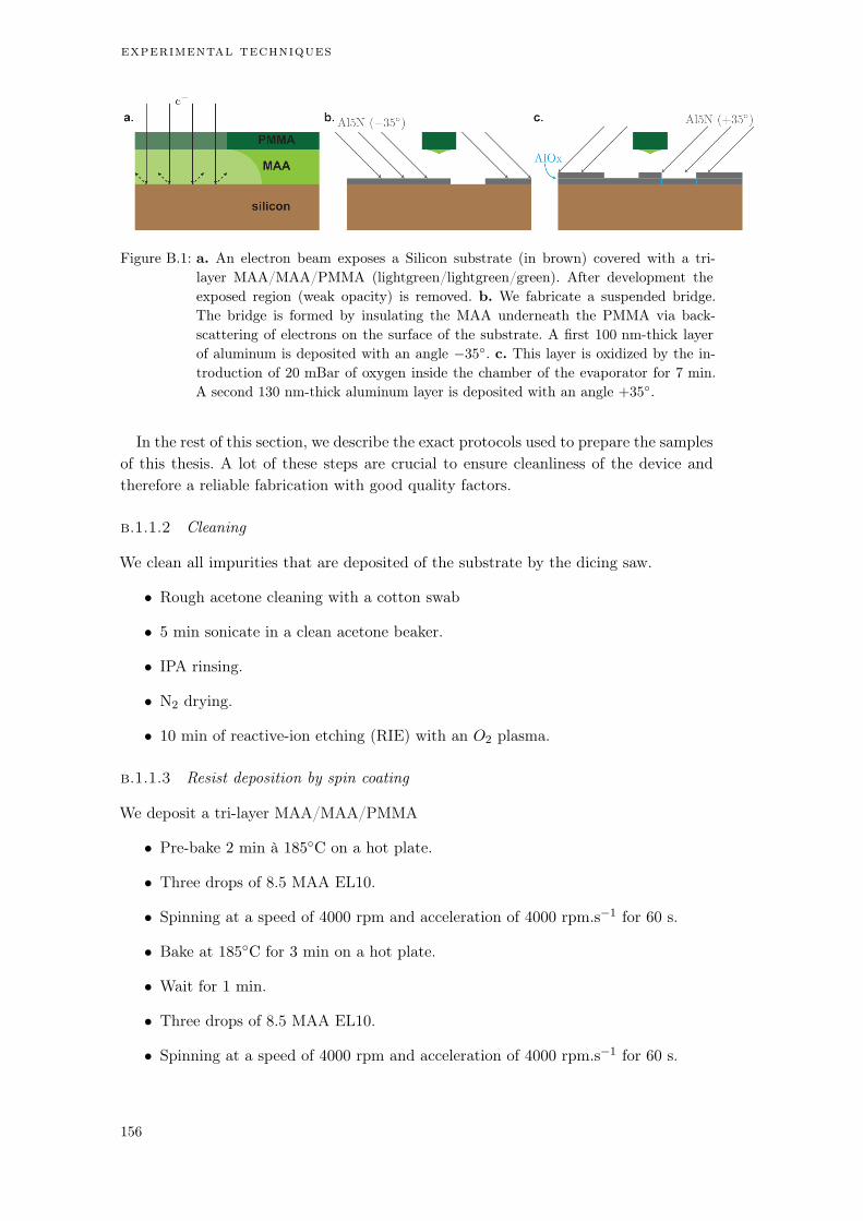
experimental techniques
Figure B.1: a. An electron beam exposes a Silicon substrate (in brown) covered with a tri-
layer MAA/MAA/PMMA (lightgreen/lightgreen/green). After development the
exposed region (weak opacity) is removed. b. We fabricate a suspended bridge.
The bridge is formed by insulating the MAA underneath the PMMA via back-
scattering of electrons on the surface of the substrate. A first 100 nm-thick layer
of aluminum is deposited with an angle 35. c. This layer is oxidized by the in-
troduction of 20 mBar of oxygen inside the chamber of the evaporator for 7 min.
A second 130 nm-thick aluminum layer is deposited with an angle +35.
In the rest of this section, we describe the exact protocols used to prepare the samplesof this thesis. A lot of these steps are crucial to ensure cleanliness of the device andtherefore a reliable fabrication with good quality factors.
b.1.1.2 Cleaning
We clean all impurities that are deposited of the substrate by the dicing saw.
• Rough acetone cleaning with a cotton swab
• 5 min sonicate in a clean acetone beaker.
• IPA rinsing.
• N2 drying.
• 10 min of reactive-ion etching (RIE) with an O2 plasma.
b.1.1.3 Resist deposition by spin coating
We deposit a tri-layer MAA/MAA/PMMA
• Pre-bake 2 min à 185C on a hot plate.
• Three drops of 8.5 MAA EL10.
• Spinning at a speed of 4000 rpm and acceleration of 4000 rpm.s1 for 60 s.
• Bake at 185C for 3 min on a hot plate.
• Wait for 1 min.
• Three drops of 8.5 MAA EL10.
• Spinning at a speed of 4000 rpm and acceleration of 4000 rpm.s1 for 60 s.
156
B.1 fabrication
• Bake at 185C for 3 min on a hot plate.
• Wait for 1 min.
• Three drops of 950 PMMA A6.
• Spinning at a speed of 4000 rpm and acceleration of 4000 rpm.s1 for 60 s.
• Bake at 185C for 3 min on a hot plate.
• Wait for 1 min.
b.1.1.4 E-beam lithography
We realize this crucial step with the Fei Magellan SEM available at ESPCI3. Thecomplete pattern is done in a single step lithography. We use two sets of parameters,the first one is used to write the Josephson junction very precisely and the second oneis used to write the rest of the circuit with a lower precision.
• We write the junction (typically about 500 nm 2 µs in area) with an electriccurrent of 9 pA accelerated by a voltage of 25 kV. The magnification is set to 600
with write fields of 100 µm and the pattern is exposed with a dose of 283 µC/cm2.
• The resonators and coupling capacitances are written with an electric current of23.5 nA accelerated by a voltage of 25 kV. The magnification is chosen to be 75
with write fields of 800 µm and the pattern is exposed with a dose of 283 µC/cm2.
b.1.1.5 Development
The development step aims at removing the exposed resist before an evaporation ofaluminum. A small quantity of resist remaining after development could lead to nonradiative loss in the device. The choice of the solution called developer used for thisstep is thus crucial to prevent residues of resist. On the opposite, if the developer istoo agressive, large undercuts grow, and may jeopardize the robustness of the Dolanbridge.
We used two different developers, a mixture of MIBK and IPA and a mixture of IPAand H2O. The former is the most widespread. It leads to a fast but imperfect removalof the resist (see Fig. B.2). In constrat, IPA/H2O is slow which leads to variation inthe development time and it is also very sensitive to variations of temperature.
development mibk/ipa
• 43 s of stirring in a solvent MIBK:IPA (1:3).
• IPA rinsing.
• N2 drying.
3 École supérieure de physique et de chimie industrielles de la ville de Paris.
157

experimental techniques
a. b.
Figure B.2: a. Optical image of an area with residues of resist after a MIBK/IPA development.
The resist leftovers prevent an homogeneous deposition of aluminum. b. Optical
image of the same area as in a but after a IPA/H2O development. The residues of
resist are gone.
development IPA/H2O
• Between 3 min 30 s et 7 min of stirring in a cold4 solvent IPA : H2O (1:3).
• IPA rinsing.
• N2 drying.
b.1.1.6 Evaporation and lift-off
The shadow evaporation technique enables us to create reproducible Josephson junc-tions by a successive deposition of two aluminum layers (100 nm and 130 nm respec-tively) interleaved by an oxide barrier. We use University Paris-Diderot clean roomfacility (see Fig. B.3 a) to deposit high purity aluminum. The chip edges are protectedwith kapton tape to avoid a direct electrical contact between the aluminum and thegold ground plane.
evaporation
• pumping for 45min to reach an evaporation chamber pressure p 3.106 mbar.
• 2 s of ion etching under 35 (500 V, 100 V, 50 mA, 12 sccn ArO2).
• 2 s of ion etching under +35.
• Evaporation of the first 130 nm-thick layer of aluminum under an angle of 35
at a rate 1 nm/s .
• 7 min of static oxidation in 20 mbar of Ar : O2 (80% Ar 20% O2)
• Evaporation of the second 100 nm-thick layer of aluminum under an angle of+35 at a rate 1 nm/s .
• Introduction of 40 mbar of ArO2 before venting.
4 Ideally, the temperature should be fixed at 4.5C thanks to a temperature controlled water bath.
158

B.1 fabrication
lift-off Finally, we remove the non exposed resist with acetone.
• at least 10 min in an acetone bath at 60C.
• 2 s sonicate in a clean acetone beaker.
• IPA rinsing.
• N2 drying.
a. b.
JJ
Figure B.3: a. Picture of a silicon chip before evaporation in a Plassys machine MEB550S. b.
Electrical scheme of a wafer prober. A ballast resistor of 1 kΩ protects the sample
by limiting the current flowing across the junction. The current is ramped up with
a potentiometer.
b.1.1.7 Wafer probing
The Ambegaokar-Baratoff relation links the normal state resistance of a junction atzero temperature R0
n to the critical current of the junction I0
R0n =
∆
2eI0=∆'0
2eEJ(B.1)
where e is the elementary charge, ∆ is the superconducting gap, '0 = ~/2e is thereduced flux quantum and EJ is the Josephson energy. The superconducting gap isof the order ∆ 180 µeV for thin film of aluminum. We estimate the resistance atzero temperature R0
n to be approximatively 20% smaller than the room temperatureresistance Rn. Measuring the resistance of a Junction at room temperature with thesetup of Fig. B.3 b gives an estimate on the Josephson energy EJ .
The wafer prober is an essential tool to select devices that are not shorted nor open5
and that display the closest EJ to the targeted value6.
5 For a SQUID, measuring twice the expected resistance indicates that one of the junction is an open.6 The Josephson energy plays an important role in the participation ratio of an amplifier (see chapter
5) or the resonant frequency of a transmon (see chapter 2).
159
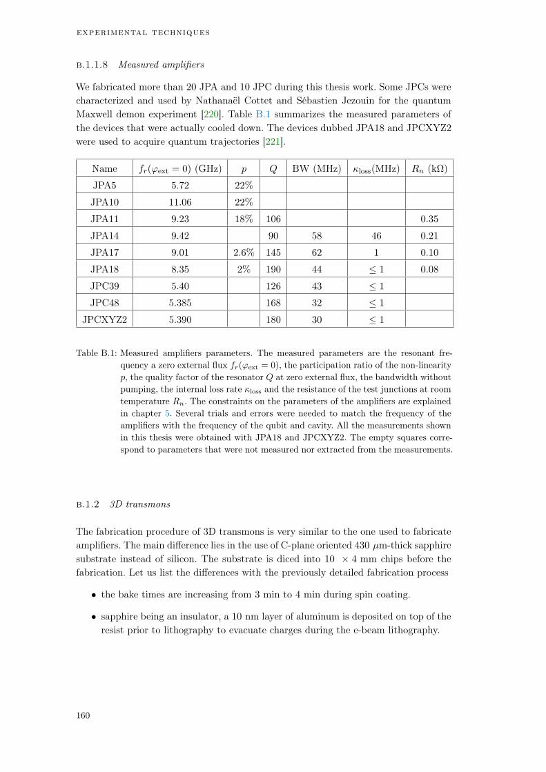
experimental techniques
b.1.1.8 Measured amplifiers
We fabricated more than 20 JPA and 10 JPC during this thesis work. Some JPCs werecharacterized and used by Nathanaël Cottet and Sébastien Jezouin for the quantumMaxwell demon experiment [220]. Table B.1 summarizes the measured parameters ofthe devices that were actually cooled down. The devices dubbed JPA18 and JPCXYZ2were used to acquire quantum trajectories [221].
Name fr('ext = 0) (GHz) p Q BW (MHz) loss(MHz) Rn (kΩ)
JPA5 5.72 22%
JPA10 11.06 22%
JPA11 9.23 18% 106 0.35
JPA14 9.42 90 58 46 0.21
JPA17 9.01 2.6% 145 62 1 0.10
JPA18 8.35 2% 190 44 1 0.08
JPC39 5.40 126 43 1
JPC48 5.385 168 32 1
JPCXYZ2 5.390 180 30 1
Table B.1: Measured amplifiers parameters. The measured parameters are the resonant fre-
quency a zero external flux fr('ext = 0), the participation ratio of the non-linearity
p, the quality factor of the resonator Q at zero external flux, the bandwidth without
pumping, the internal loss rate loss and the resistance of the test junctions at room
temperature Rn. The constraints on the parameters of the amplifiers are explained
in chapter 5. Several trials and errors were needed to match the frequency of the
amplifiers with the frequency of the qubit and cavity. All the measurements shown
in this thesis were obtained with JPA18 and JPCXYZ2. The empty squares corre-
spond to parameters that were not measured nor extracted from the measurements.
b.1.2 3D transmons
The fabrication procedure of 3D transmons is very similar to the one used to fabricateamplifiers. The main difference lies in the use of C-plane oriented 430 µm-thick sapphiresubstrate instead of silicon. The substrate is diced into 10 4 mm chips before thefabrication. Let us list the differences with the previously detailed fabrication process
• the bake times are increasing from 3 min to 4 min during spin coating.
• sapphire being an insulator, a 10 nm layer of aluminum is deposited on top of theresist prior to lithography to evacuate charges during the e-beam lithography.
160

B.1 fabrication
• this thin aluminum layer is removed after e-beam writing and before developmentby immersion of the chip in a KOH solution7.
• we deposit a first layer of 35 nm of aluminum (instead of 100 nm) followed byoxidation and a second layer of 100 nm (instead of 130 nm) of aluminum duringthe evaporation.
The other steps are unchanged. Luckily, the first transmon that we cooled down had suf-ficiently good coherence times for our experiments. It was used for all the measurementspresented in this manuscript.
b.1.3 2D CPW chips
We also used 2D circuits composed of several microwave resonators and qubits. Theresonators and qubits are patterned in the coplanar waveguide geometry. The associatedexperiments are still on-going and the results are not presented in the manuscript.Nevertheless, we describe the fabrication process used to make our 2D chips. Thesechips were fabricated by Théau Peronnin and Raphaël Lescanne at ENS Paris with aprocess developed jointly with Danijela Marković [149].
After cleaning the wafer, a 150 nm layer of of Nb is deposited on the entire uppersurface of the substrate by sputtering. The resonators, geometric inductances and ca-pacitances are patterned by optical lithography with the laser writer available in theclean room at Collège de France. After development, the niobium is dry etched usingSF6 to form the ‘gaps’ of the CPW. Aluminum Josephson junction are written at theend by e-beam lithography. Let us briefly describe the fabrication process.
spin coating
• One drop of S1813.
• Spinning at a speed of 4000 rpm for 60 s.
• Bake at 115C for 1 min on a hot plate.
optical lithography
• We use a microtech LW405-B+ laser writer.
• Exposition at a dose 300 mJ/cm2.
development
• AZ726-MIF for 90 ns
• H2O rinsing.
7 The concentration of the KOH solution (KOH comes as solid pellets) and the immersion time are notcontrolled carefully. We simply wait for the visible dissolution of the aluminum layer.
161
experimental techniques
etching
• Reactive ion etching with SF6 for 2 min.
• Dissolution of the remaining resist in acetone.
• IPA rinsing.
• N2 drying.
Josephson junctions are then written with the exact same protocol as the one usedfor 3D transmons.
b.2 measurement setup
Fig. B.4 is a picture of the inside of the dilution refrigerator used in during this thesis.Our devices are shielded by aluminum foils and placed inside cryoperm boxes. Theyare thermally anchored at the base plate of the dilution refrigerator at a temperatureof 20 mK. The signal coming from room temperature is heavily attenuated at everystage of the refrigerator and filtered by XMA attenuators and home-made eccosorbfilters to prevent any thermal noise from reaching the base plate. A special care istaken to thermally anchor all microwave components at every stage. SuperconductingNbTi coaxial cables are used on the return lines between base temperature and 4 K
to minimize the losses before the HEMT while reducing the heat exchange betweenthese stages. Twisted DC lines are used to current biais coils that are placed above theamplifiers to enable us to match the frequency of the amplifiers with our qubit andcavity.
Fig. B.5 is a diagram of the measurement setup. The qubit-cavity system describedthroughout this thesis is probed via coaxial transmission lines whose central pin plungeinto the 3D cavity. Readout and qubit drive and gate are produced by mixing a fewGHz continuous wave with 50 MHz (readout) and 40 MHz (qubit) modulated pulsesgenerated by a Tektronix AWG8 5014C. At the output of the cavity, a commercial9
frequency diplexer routes output signal in the frequency range DC 7 GHz (includingqubit frequency) toward a Josephson parametric converter (JPC). The signal in thefrequency range 7 GHz 14 GHz is routed toward a Josephson parametric amplifier(JPA). The JPA is double pumped by two side-bands generated by an IQ mixing of thereadout frequency. The two spatially separated detection chains are further amplifiedby a HEMT10 at 4 K and at room temperature before down conversion, digitization byan Alazar 9351 ADC board and numerical demodulation. Several cryogenic circulatorsare used to prevent amplified noise from entering the cavity from the output port andthus degrade the qubit coherence time (see chapter 5).
8 Arbitrary waveform generator.9 TIGER TGF-A4214-001.
10 Low Noise Factory high electron mobility transistor amplifiers.
162

B.2 measurement setup
circulators
a.
b.
850 mK
100 mK
20 mK
4 K
attenuators
cryoperm shieldseccosorb filter
K&L filter
DC lines
Nb-Ti coax
thermalization
copper braid
Figure B.4: Wiring of our BlueFors dilution refrigerator for several experiments. a. Wiring of
the fridge between 4 K and base temperature. The signal coming from room tem-
perature is heavily attenuated and filtered to prevent thermal noise from reaching
the base plate. b. Zoom on the 20 mK stage. Qubits and amplifiers placed inside
cryoperm boxes and thermally anchored to the base plate of the dilution refrigera-
tor with copper braids.
163

experimental techniques
Δ
Σ
3D transmon
4K
70K
RT
50
100mK
850mK
20mK
in out
JPC
JPA
50
-20dB
LPF
Eccosorb
-20dB
-10dB
-20dB
LPF
Eccosorb
-10dB
-10dB
-20dB
LPF
Eccosorb
-20dB
-10dB
-20dB
LPF
Eccosorb-1
0dB
-10dB
50
50
50
50
LNF
+40dB
50
50
50
Diplexer
LNF
+40dB
reflection
probe
Δ
Σ
LPF
Eccosorb
LPF
Eccosorb
50
readout
50
AW
G
SSB
50
50
AD
C
50
50
I Q
AW
G
AW
G
+20dB +20dB
JPC
pump
qubit drive
AW
G
SSB
AD
C
50
50
50
Figure B.5: Schematics of the experimental setup for the quantum trajectories experiment. A
single RF source at fc /2+ 50 MHz is used to readout the cavity by single side
band modulation and to generate a two side-band pump for a JPA. The mixed
readout signal is sent through the input line which is heavily attenuated (XMA at-
tenuators) and filtered with home made ecosorb filters. At the output of the cavity
a commercial frequency diplexer routes the signal toward a Josphson parametric
converter (JPC)(frequencies lower than 7 GHz including fq) or a Josephson para-
metric amplifier (JPA) (frequencies higher than 7 GHz including fc). The readout
pulse is further amplified by a HEMT routed out of the fridge before down con-
version, digitization and numerical demodulation. An additional tone is mixed at
40 MHz and used for qubit rotations and down conversion of the amplified fluores-
cence field at room. The fluorescence signal is also digitized and demodulated to
extract the two associated measurement records.164

Part IV
B IBL IOGRAPHY


BIBL IOGRAPHY
[1] A Pais. “Einstein and the quantum theory.” In: Reviews of Modern Physics 51.4(1979), pp. 863–914. arXiv: 0510180 [quant-ph] (Cited on page 1).
[2] A Einstein, B Podolsky, and N Rosen. “Can Quantum-Mechanical Descriptionof Physical Reality Be Considered Complete?” In: Physical Review 47 (1935),p. 777. arXiv: 0701001 [quant-ph] (Cited on page 1).
[3] David Bohm. “A suggested interpretation of the quantum theory in terms of"hidden" variables. I.” In: Physical Review (1952). arXiv: 0208158 [quant-ph]
(Cited on page 1).
[4] Stuart J Freedman and John F Clauser. “Experimental Test of Local Hidden-Variable Theories.” In: Phys. Rev. Lett. 28.14 (1972), pp. 938–941 (Cited onpage 1).
[5] Alain Aspect, Jean Dalibard, and Gérard Roger. “Experimental Test of Bell’sInequalities Using Time- Varying Analyzers.” In: Physical Review Letters 49.25(1982), pp. 1804–1807 (Cited on page 1).
[6] Erwin Schrödinger. The Present Situation in Quantum Mechanics. 1980. arXiv:1206.6024 (Cited on page 1).
[7] Zurek. “Decoherence, einselection, and the quantum origins of the classical.” In:Reviews of Modern Physics 75.3 (2003), pp. 715–775 (Cited on pages 1, 32).
[8] Max Jammer. The Philosophy of Quantum Mechanics. New York: Wiley, 1974(Cited on page 2).
[9] Lucien Hardy and Robert Spekkens. “Why Physics Needs Quantum Founda-tions.” In: (). arXiv: arXiv:1003.5008v1 (Cited on page 2).
[10] E. Schrödinger. “Are there quantum jumps ?: Part ii.” In: British Journal forthe Philosophy of Science (1952) (Cited on page 2).
[11] Rainer Blatt and David Wineland. Entangled states of trapped atomic ions. 2008(Cited on page 3).
[12] Serge Haroche. “Nobel Lecture: Controlling photons in a box and exploringthe quantum to classical boundary.” In: Reviews of Modern Physics 85 (2013),p. 1083 (Cited on pages 3, 13).
[13] M. H. Devoret et al. “Superconducting circuits for quantum information: An out-look.” In: Science 339.6124 (2013), pp. 1169–1174. arXiv: 0402594 [cond-mat]
(Cited on pages 3, 14).
[14] Leo Kouwenhoven and Charles Marcus. “Quantum dots.” In: Physics World(1998). arXiv: 1412.1667 (Cited on page 3).
[15] Markus Aspelmeyer, Tobias J. Kippenberg, and Florian Marquardt. “Cavityoptomechanics.” In: Reviews of Modern Physics (2014). arXiv: 1303.0733 (Citedon page 3).
167

bibliography
[16] John M. Martinis, Michel H. Devoret, and John Clarke. “Experimental tests forthe quantum behavior of a macroscopic degree of freedom: The phase differenceacross a Josephson junction.” In: Physical Review B (1987) (Cited on page 3).
[17] Y. Nakamura, Yu. a. Pashkin, and J. S. Tsai. “Coherent control of macro-scopic quantum states in a single-Cooper-pair box.” In: Nature 398.6730 (1999),pp. 786–788. arXiv: 9904003 [cond-mat] (Cited on pages 3, 13, 21).
[18] Uri Vool and Michel Devoret. “Introduction to quantum electromagnetic cir-cuits.” In: International Journal of Circuit Theory and Applications. 2017. arXiv:1610.03438 (Cited on page 3).
[19] Jens Koch et al. “Charge-insensitive qubit design derived from the Cooper pairbox.” In: Physical Review A - Atomic, Molecular, and Optical Physics 76.4(2007), p. 042319. arXiv: 0703002 [cond-mat] (Cited on pages 3, 14, 23, 35,40).
[20] J. A. Schreier et al. “Suppressing charge noise decoherence in superconductingcharge qubits.” In: Physical Review B - Condensed Matter and Materials Physics77.18 (2008), p. 180502. arXiv: 0712.3581 (Cited on pages 3, 14, 23).
[21] John M. Martinis. Qubit metrology for building a fault-tolerant quantum com-puter . 2015. arXiv: 1510.01406 (Cited on page 3).
[22] A Wallraff et al. “Strong coupling of a single photon to a superconducting qubitusing circuit quantum electrodynamics.” In: Nature 431 (2004), pp. 162–167(Cited on pages 4, 13).
[23] P Campagne-Ibarcq et al. “Observing quantum state diffusion by heterodynedetection of fluorescence.” In: Physical Review X 6.1 (2016), p. 11002. arXiv:1511.01415 (Cited on pages 4, 6, 45, 98, 105, 115, 129).
[24] M. Naghiloo et al. “Mapping quantum state dynamics in spontaneous emission.”In: Nature Communications 7.May (2016), pp. 1–7. arXiv: 1512.02307 (Citedon pages 4, 115).
[25] M. Naghiloo et al. “Quantum caustics in resonance-fluorescence trajectories.”In: Physical Review A (2017). arXiv: 1612.03189 (Cited on pages 4, 6, 98, 115,132).
[26] M Hatridge et al. “Quantum Back-Action of an Individual Variable-StrengthMeasurement.” In: Science 339.6116 (2013), pp. 178–181 (Cited on pages 4, 6,47, 98).
[27] K W Murch et al. “Observing single quantum trajectories of a superconductingquantum bit.” In: Nature 502.7470 (2013), pp. 211–214. arXiv: 1305.7270 (Citedon pages 4, 6, 98, 100, 102, 115).
[28] G de Lange et al. “Reversing Quantum Trajectories with Analog Feedback.” In:Physical Review Letters 112.8 (2014), p. 80501 (Cited on pages 4, 6, 98, 103).
[29] Steven J Weber et al. “Quantum trajectories of superconducting qubits.” In:Comptes Rendus Physique 17.7 (2016), pp. 766–777 (Cited on pages 4, 6, 98).
[30] P Facchi et al. “Quantum Zeno dynamics.” In: Physics Letters A 275.1-2 (2000),pp. 12–19 (Cited on pages 5, 115).
168

bibliography
[31] J Gough. “Zeno dynamics for open quantum systems.” In: Russian Journal ofMathematical Physics 21.3 (2014), pp. 337–347 (Cited on pages 5, 115).
[32] B Yurke et al. “Observation of parametric amplification and deamplification ina Josephson parametric amplifier.” In: Physical Review A 39.5 (1989), p. 2519(Cited on pages 5, 73, 75).
[33] M A Castellanos-Beltran and K W Lehnert. “Widely tunable parametric ampli-fier based on a superconducting quantum interference device array resonator.”In: Applied Physics Letters 91.8 (2007), p. 83509 (Cited on pages 5, 75, 76).
[34] T Yamamoto et al. “Flux-driven Josephson parametric amplifier.” In: AppliedPhysics Letters 93.4 (2008), p. 42510 (Cited on pages 5, 75).
[35] Archana Kamal, Adam Marblestone, and Michel Devoret. “Signal-to-pump backaction and self-oscillation in double-pump Josephson parametric amplifier.” In:Physical Review B 79.18 (2009), p. 184301. arXiv: 0902.0007 (Cited on pages 5,75).
[36] J Y Mutus et al. “Strong environmental coupling in a Josephson parametricamplifier.” In: Applied Physics Letters 104.26 (2014), p. 263513 (Cited on pages 5,75).
[37] Christopher Eichler and Andreas Wallraff. “Controlling the dynamic range of aJosephson parametric amplifier.” In: EPJ Quantum Technology 1.1 (2014), p. 2(Cited on pages 5, 75).
[38] N Bergeal et al. “Analog information processing at the quantum limit with aJosephson ring modulator.” In: Nature Physics 6.4 (2010), pp. 296–302 (Citedon pages 5, 81).
[39] N. Roch et al. “Widely Tunable, Nondegenerate Three-Wave Mixing MicrowaveDevice Operating near the Quantum Limit.” In: Physical Review Letters 108.14(2012), p. 147701. arXiv: arXiv:1202.1315v1 (Cited on pages 5, 81, 84, 86).
[40] Emmanuel Flurin. “The Josephson Mixer, a Swiss army knife for microwavequantum optics.” Theses. ENS, 2014 (Cited on pages 5, 81–83, 90, 91, 155).
[41] N. Gisin and I. C. Percival. “The quantum-state diffusion model applied to opensystems.” In: Journal of Physics A: General Physics 25.21 (1992), pp. 5677–5691(Cited on pages 6, 97).
[42] H Carmichael. An Open Systems Approach to Quantum Optics . Springer BerlinHeidelberg, 1993 (Cited on pages 6, 97).
[43] Christine Guerlin et al. “Progressive field-state collapse and quantum non-demolitionphoton counting.” In: Nature 448.7156 (2007), pp. 889–893 (Cited on pages 6,97).
[44] Howard M Wiseman and G J Milburn. Quantum Measurement and Control.Cambridge University Press, 2009 (Cited on pages 6, 36, 41, 97, 99).
[45] Alberto Barchielli and Matteo Gregoratti. Quantum Trajectories and Measure-ments in Continuous Time. Vol. 782. Springer-Verlag Berlin Heidelberg, 2009(Cited on pages 6, 97).
169
bibliography
[46] Alexander N Korotkov. “Quantum Bayesian approach to circuit QED mea-surement.” In: Les Houches summer school "Quantum Machines" (2011). 2011.arXiv: 1111.4016 (Cited on pages 6, 97).
[47] D Ristè et al. “Deterministic entanglement of superconducting qubits by paritymeasurement and feedback.” In: Nature 502.7471 (2013), pp. 350–354 (Cited onpages 6, 98).
[48] N. Roch et al. “Observation of measurement-induced entanglement and quan-tum trajectories of remote superconducting qubits.” In: Physical Review Letters112.17 (2014). arXiv: 1402.1868 (Cited on pages 6, 98).
[49] Shay Hacohen-Gourgy et al. “Dynamics of simultaneously measured non-commutingobservables.” In: Nature 538 (2016), p. 491. arXiv: 1608.06652 (Cited on pages 6,8, 92, 98, 115, 119, 129, 131, 132).
[50] Andrew N. Jordan and Markus Báttiker. “Continuous quantum measurementwith independent detector cross correlations.” In: Physical Review Letters (2005)(Cited on page 8).
[51] Michel Bauer, Denis Bernard, and Antoine Tilloy. “The open quantum Brownianmotions.” In: Journal of Statistical Mechanics: Theory and Experiment 2014.9(2014). arXiv: 1312.1600 (Cited on pages 8, 123).
[52] J von Neumann and R T Beyer. Mathematical Foundations of Quantum Me-chanics. Investigations in physics. Princeton University Press, 1996 (Cited onpages 8, 133).
[53] D Bohm. Quantum Theory. Dover books in science and mathematics. DoverPublications, 1989 (Cited on pages 8, 133).
[54] Yakir Aharonov, Peter Bergmann, and Joel Lebowitz. “Time Symmetry in theQuantum Process of Measurement.” In: Physical Review 134.6B (1964), B1410–B1416 (Cited on pages 8, 133).
[55] H. M. Wiseman. “Weak values, quantum trajectories, and the cavity-QED exper-iment on wave-particle correlation.” In: Physical Review A 65.3 (2002), p. 32111.arXiv: 0112116 [quant-ph] (Cited on pages 8, 133, 134, 137, 138).
[56] Mankei Tsang. “Optimal waveform estimation for classical and quantum systemsvia time-symmetric smoothing. II. Applications to atomic magnetometry andHardy’s paradox.” In: Physical Review A 81.3 (2009), p. 33840 (Cited on pages 8,133, 134).
[57] Mankei Tsang. “Time-Symmetric Quantum Theory of Smoothing.” In: PhysicalReview Letters 102.25 (2009), p. 250403 (Cited on pages 8, 133, 134).
[58] Søren Gammelmark, Brian Julsgaard, and Klaus Mølmer. “Past Quantum Statesof a Monitored System.” In: Physical Review Letters 111.16 (2013), p. 160401(Cited on pages 8, 133, 134, 136, 137, 145).
[59] Yakir Aharonov, David Albert, and Lev Vaidman. “How the result of a measure-ment of a component of the spin of a spin-1/2 particle can turn out to be 100.”In: Physical Review Letters 60.14 (1988), pp. 1351–1354 (Cited on pages 9, 133,138, 141).
170
bibliography
[60] Justin Dressel et al. “Colloquium: Understanding quantum weak values: Ba-sics and applications.” In: Reviews of Modern Physics 86.1 (2014), pp. 307–316.arXiv: 1305.7154 (Cited on pages 9, 133, 134, 140, 142, 145).
[61] Nathan Williams and Andrew Jordan. “Weak Values and the Leggett-Garg In-equality in Solid-State Qubits.” In: Physical Review Letters 100.2 (2008), p. 26804(Cited on pages 9, 133, 141).
[62] Philippe Campagne-Ibarcq et al. “Observing interferences between past andfuture quantum states in resonance fluorescence.” In: Physical Review Letters112.18 (2014), pp. 1–5. arXiv: arXiv:1311.5605v1 (Cited on pages 9, 133).
[63] D. Tan et al. “Prediction and retrodiction for a continuously monitored supercon-ducting qubit.” In: Physical Review Letters 114.9 (2015), p. 6. arXiv: 1409.0510(Cited on pages 9, 133, 145).
[64] D. Tan et al. “Homodyne monitoring of postselected decay.” In: Physical ReviewA (2017). arXiv: 1705.04287 (Cited on pages 9, 133, 145).
[65] David J. Wineland. Superposition, entanglement, and raising Schrödinger’s cat .2013 (Cited on page 13).
[66] S Haroche and J Raimond. “Exploring the Quantum: Atoms, Cavities, and Pho-tons.” In: Oxford Graduated Text (2006), p. 616 (Cited on pages 13, 18, 36, 38,47, 48).
[67] Hanhee Paik et al. “Observation of High Coherence in Josephson Junction QubitsMeasured in a Three-Dimensional Circuit QED Architecture.” In: Physical Re-view Letters 107.24 (2011), p. 240501 (Cited on pages 14, 15).
[68] Austin G Fowler et al. “Surface codes: Towards practical large-scale quantumcomputation.” In: Physical Review A 86.3 (2012), p. 32324 (Cited on page 14).
[69] Mazyar Mirrahimi et al. “Dynamically protected cat-qubits: a new paradigmfor universal quantum computation.” In: New Journal of Physics 16.4 (2014),p. 45014. arXiv: arXiv:1312.2017v1 (Cited on page 14).
[70] L. Dicarlo et al. “Demonstration of two-qubit algorithms with a superconductingquantum processor.” In: Nature 460.7252 (2009), pp. 240–244. arXiv: 0903.2030(Cited on page 14).
[71] R Barends et al. “Superconducting quantum circuits at the surface code thresh-old for fault tolerance.” In: Nature 508.7497 (2014), pp. 500–503 (Cited onpages 14, 35).
[72] Matthew Reagor et al. “Reaching 10 ms single photon lifetimes for supercon-ducting aluminum cavities.” In: Applied Physics Letters 102.19 (2013), p. 192604(Cited on page 15).
[73] M Devoret. “Quantum fluctuations in electrical circuits.” In: Les Houches (1995)(Cited on pages 14, 21).
[74] S Girvin. “Circuit QED: superconducting qubits coupled to microwave photons.”In: Quantum Machines: Measurement and Control of Engineered Quantum Sys-tems, Lecture notes of the Les Houches Summer School: volume 96. Ed. by MichelDevoret et al. Oxford University Press, USA, 2014, p. 113 (Cited on page 14).
171
bibliography
[75] D M Pozar. Microwave Engineering. Wiley, 2004 (Cited on pages 14, 155).
[76] Matthew Reagor. “Superconducting Cavities for Circuit Quantum Electrody-namics.” PhD thesis. 2015 (Cited on pages 14, 19).
[77] John Preskill. “Preskills Lectures.” In: Quantum Computing - Physics 219 Lec-ture notes (2001). arXiv: 0101025v2 [arXiv:quant-ph] (Cited on page 18).
[78] Alexandre Blais et al. “Cavity quantum electrodynamics for superconductingelectrical circuits: An architecture for quantum computation.” In: Physical Re-view A 69.6 (2004), p. 062320. arXiv: 0402216 [cond-mat] (Cited on page 19).
[79] S Kuhr et al. “Ultrahigh finesse Fabry-Perot superconducting resonator.” In:Applied Physics Letters 90.16 (2007), p. 164101 (Cited on page 19).
[80] V. Bouchiat et al. “Quantum Coherence with a Single Cooper Pair.” In: PhysicaScripta T76.1 (1998), p. 165 (Cited on page 21).
[81] K. W. Lehnert et al. “Measurement of the Excited-State Lifetime of a Micro-electronic Circuit.” In: Physical Review Letters (2003) (Cited on page 21).
[82] Simon E Nigg et al. “Black-box superconducting circuit quantization.” In: Physi-cal Review Letters 108.24 (2012), p. 240502. arXiv: 1204.0587 (Cited on pages 24,25, 149).
[83] Firat Solgun, David W. Abraham, and David P. Divincenzo. “Blackbox quanti-zation of superconducting circuits using exact impedance synthesis.” In: Phys-ical Review B - Condensed Matter and Materials Physics 90.13 (2014). arXiv:1403.7341 (Cited on page 24).
[84] Moein Malekakhlagh and Hakan E. Türeci. “Origin and implications of an A2-like contribution in the quantization of circuit-QED systems.” In: Physical Re-view A (2016). arXiv: 1506.02773 (Cited on page 24).
[85] Philippe Campagne-Ibarcq. “Measurement back action and feedback in super-conducting circuits.” Thesis. ENS, 2015 (Cited on pages 24, 47, 61, 105, 137,140, 155).
[86] Kurtis Lee Geerlings. “Improving Coherence of Superconducting Qubits andResonators.” PhD thesis (Cited on pages 26, 61).
[87] John David Jackson. Jackson - Classical Electrodynamics (3rd Ed.).pdf . 1962(Cited on page 28).
[88] Z Leghtas et al. “Confining the state of light to a quantum manifold by en-gineered two-photon loss.” In: Science 347.6224 (2015), pp. 853–857. arXiv:1412.4633 (Cited on pages 29, 71).
[89] Z. K. Minev et al. “Planar Multilayer Circuit Quantum Electrodynamics.” In:Physical Review Applied (2016). arXiv: 1509.01619 (Cited on page 29).
[90] S. Touzard et al. “Coherent Oscillations inside a Quantum Manifold Stabilizedby Dissipation.” In: Physical Review X (2018). arXiv: 1705.02401 (Cited onpage 29).
172
bibliography
[91] J.-M. Raimond. “Exploring the quantum world with photons trapped in cavi-ties and Rydberg atoms.” In: Quantum Machines: Measurement and Control ofEngineered Quantum Systems (2014), pp. 395–426 (Cited on page 29).
[92] M. Nielsen and I. L. Chuang. Quantum Computation and Quantum Information:10th Anniversary Edition. 2010. arXiv: arXiv:1011.1669v3 (Cited on pages 31,37).
[93] Nicolas Gisin and Ian C Percival. “The quantum state diffusion picture of phys-ical processes.” In: Journal of Physics A 26 (1993), p. 2245 (Cited on page 32).
[94] David P DiVincenzo. “Fault-tolerant architectures for superconducting qubits.”In: Physica Scripta T137 (2009), p. 14020 (Cited on page 35).
[95] M D Reed et al. “Fast reset and suppressing spontaneous emission of a super-conducting qubit.” In: Applied Physics Letters 96.20 (2010), p. 203110 (Citedon page 35).
[96] T. Walter et al. “Rapid High-Fidelity Single-Shot Dispersive Readout of Super-conducting Qubits.” In: Physical Review Applied (2017). arXiv: 1701.06933
(Cited on page 35).
[97] Johannes Heinsoo et al. “Rapid High-fidelity Multiplexed Readout of Super-conducting Qubits.” In: Physical Review Applied 10.3 (2018), pp. 1–13. arXiv:1801.07904 (Cited on page 35).
[98] T. Picot et al. “Role of relaxation in the quantum measurement of a supercon-ducting qubit using a nonlinear oscillator.” In: Physical Review B - CondensedMatter and Materials Physics (2008). arXiv: 0808.0464 (Cited on page 35).
[99] Daniel Sank et al. “Measurement-Induced State Transitions in a Superconduct-ing Qubit: Beyond the Rotating Wave Approximation.” In: Physical ReviewLetters (2016). arXiv: 1606.05721 (Cited on page 35).
[100] I Siddiqi et al. “RF-Driven Josephson Bifurcation Amplifier for Quantum Mea-surement.” In: Physical Review Letters 93.20 (2004), p. 207002 (Cited on pages 35,74).
[101] F Mallet et al. “Single-shot qubit readout in circuit quantum electrodynamics.”In: Nature Physics 5.11 (2009), pp. 791–795 (Cited on page 35).
[102] M D Reed et al. “High-Fidelity Readout in Circuit Quantum ElectrodynamicsUsing the Jaynes-Cummings Nonlinearity.” In: Physical Review Letters 105.17(2010), p. 173601 (Cited on page 35).
[103] Th K. Mavrogordatos et al. “Simultaneous Bistability of a Qubit and Resonatorin Circuit Quantum Electrodynamics.” In: Physical Review Letters 118.4 (2017),pp. 1–5. arXiv: 1611.10354 (Cited on page 35).
[104] I. Pietikäinen et al. “Multilevel Effects in a Driven Generalized Rabi Model.”In: Journal of Low Temperature Physics 191.5-6 (2018), pp. 354–364. arXiv:1710.00588 (Cited on page 35).
[105] Raphaël Lescanne et al. “Dynamics of an off-resonantly pumped superconductingqubit in a cavity.” In: arXiv:1805.05198 (2018). arXiv: 1805.05198 (Cited onpages 35, 56, 69).
173

bibliography
[106] S. Touzard et al. “Gated conditional displacement readout of superconductingqubits.” In: arXiv:1809.06964 (2018). arXiv: 1809.06964 (Cited on page 35).
[107] Claude Cohen-Tannoudji, Bernard Diu, and Franck Laloe. Quantum Mechanics- Vol 1 - Cohen-Tannoudji.pdf. 2006 (Cited on page 36).
[108] Mazyar Mirrahimi and Pierre Rouchon. “Dynamics and Control of Open Quan-tum Systems.” In: 2015 (Cited on pages 36, 108).
[109] A. Uhlmann. “Relative entropy and the Wigner-Yanase-Dyson-Lieb concavity inan interpolation theory.” In: Communications in Mathematical Physics (1977)(Cited on page 38).
[110] A. Barchielli M. and M. Gregoratti. “Quantum Trajectories and Measurementsin Continuous Time: The Diffusive Case.” In: Springer (2009) (Cited on page 39).
[111] Mark Fox. “Quantum Optics.” In: University of Oxford (2013). arXiv: arXiv:1011.1669v3 (Cited on pages 39, 45).
[112] A. Wallraff et al. “Approaching unit visibility for control of a superconduct-ing qubit with dispersive readout.” In: Physical Review Letters (2005). arXiv:0502645 [cond-mat] (Cited on page 40).
[113] Jay Gambetta et al. “Quantum trajectory approach to circuit QED: Quantumjumps and the Zeno effect.” In: Physical Review A 77.1 (2008), p. 12112. arXiv:0709.4264 (Cited on pages 41, 44, 57).
[114] A. A. Clerk et al. “Introduction to quantum noise, measurement, and ampli-fication.” In: Reviews of Modern Physics 82.2 (2010), pp. 1155–1208. arXiv:0810.4729 (Cited on page 42).
[115] Vijay, Slichter, and Siddiqi. “Observation of Quantum Jumps in a Supercon-ducting Artificial Atom.” In: Physical Review Letters 106.11 (2011), p. 110502(Cited on pages 42, 67).
[116] B Misra and E C G Sudarshan. “The Zeno paradox in quantum theory.” In:Journal of Mathematical Physics 18.4 (1977), p. 756 (Cited on page 42).
[117] H. J. Carmichael. “Quantum trajectory theory for cascaded open systems.” In:Physical Review Letters (1993) (Cited on page 45).
[118] R. Bianchetti et al. “Control and tomography of a three level superconductingartificial atom.” In: Physical Review Letters (2010). arXiv: 1004.5504 (Cited onpages 55, 57, 63, 64, 66).
[119] Michael J. Peterer et al. “Coherence and decay of higher energy levels of asuperconducting transmon qubit.” In: Physical Review Letters (2015). arXiv:1409.6031 (Cited on pages 55, 63, 64).
[120] A B Klimov et al. “Qutrit quantum computer with trapped ions.” In: PhysicalReview A - Atomic, Molecular, and Optical Physics 67.6 (2003), p. 7 (Cited onpage 55).
[121] Helle Bechmann-Pasquinucci and Asher Peres. “Quantum cryptography with 3-state systems.” In: Physical Review Letters (2000). arXiv: 0001083 [quant-ph]
(Cited on page 55).
174

bibliography
[122] Thomas Durt et al. “Security of quantum key distributions with entangled qu-dits.” In: Physical Review A - Atomic, Molecular, and Optical Physics 69.3(2004), pp. 1–11 (Cited on page 55).
[123] M Pechal et al. “Microwave-controlled generation of shaped single photons incircuit quantum electrodynamics.” In: arxiv:1308.4094 (2013). arXiv: 1308.4094(Cited on page 55).
[124] Anatoly Kulikov et al. “Realization of a Quantum Random Generator Certifiedwith the Kochen-Specker Theorem.” In: Physical Review Letters 119.24 (2017),pp. 1–5. arXiv: 1709.03687 (Cited on page 55).
[125] A. A. Abdumalikov et al. “Experimental realization of non-Abelian non-adiabaticgeometric gates.” In: Nature (2013). arXiv: 1304.5186 (Cited on page 55).
[126] Benjamin P. Lanyon et al. “Simplifying quantum logic using higher-dimensionalHilbert spaces.” In: Nature Physics (2009). arXiv: 0804.0272 (Cited on page 55).
[127] Frederick W. Strauch. “Quantum logic gates for superconducting resonator qu-dits.” In: Physical Review A - Atomic, Molecular, and Optical Physics (2011).arXiv: 1108.2984 (Cited on page 55).
[128] Vincent Mourik et al. “Exploring quantum chaos with a single nuclear spin.” In:arXiv:1703.04852 (2017). arXiv: 1703.04852 (Cited on page 55).
[129] A. R. Shlyakhov et al. “Quantum metrology with a transmon qutrit.” In: PhysicalReview A (2018). arXiv: 1711.06172 (Cited on page 55).
[130] J. Wenner et al. “Excitation of superconducting qubits from hot nonequilibriumquasiparticles.” In: Physical Review Letters (2013). arXiv: 1209.1674 (Cited onpage 59).
[131] K. Serniak et al. “Hot non-equilibrium quasiparticles in transmon qubits.” In:arXiv:1803.00476 (2018). arXiv: 1803.00476 (Cited on page 61).
[132] Jian Li et al. “Pure dephasing in a superconducting three-level system.” In:Journal of Physics: Conference Series 400.PART 4 (2012) (Cited on page 62).
[133] Z. Wang et al. “Cavity Attenuators for Superconducting Qubits.” In: arXiv:1807.04849(2018). arXiv: 1807.04849 (Cited on page 64).
[134] M A Castellanos-Beltran et al. “Amplification and squeezing of quantum noisewith a tunable Josephson metamaterial.” In: Nature Physics 4.12 (2008), pp. 929–931 (Cited on page 71).
[135] N Bergeal et al. “Phase-preserving amplification near the quantum limit with aJosephson ring modulator.” In: Nature 465.7294 (2010), p. 64 (Cited on pages 71,85).
[136] C Macklin et al. “A near – quantum-limited Josephson traveling-wave parametricamplifier.” In: Science 350.September (2015), p. 307 (Cited on pages 71, 86–88,92).
[137] E. Flurin et al. “Generating Entangled Microwave Radiation Over Two Trans-mission Lines.” In: Physical Review Letters 109.18 (2012), p. 183901. arXiv:1204.0732 (Cited on page 71).
175

bibliography
[138] M Pechal et al. “Microwave-Controlled Generation of Shaped Single Photonsin Circuit Quantum Electrodynamics.” In: Physical Review X 041010.4 (2014),pp. 1–9 (Cited on page 71).
[139] E Flurin et al. “Superconducting quantum node for entanglement and storageof microwave radiation.” In: Phys. Rev. Lett. 114.Umr 8551 (2014), p. 90503.arXiv: arXiv:1401.5622v1 (Cited on page 71).
[140] K W Murch et al. “Cavity-Assisted Quantum Bath Engineering.” In: PhysicalReview Letters 109.18 (2012), p. 183602 (Cited on page 71).
[141] Greg Calusine. “Private communication: TWPA Data Sheet.” 2017 (Cited onpages 71, 88, 92).
[142] C M Caves. “Quantum limits on noise in linear amplifiers.” In: Physical ReviewD 26 (1982), p. 1817 (Cited on page 72).
[143] Ananda Roy and Michel Devoret. Introduction à l’amplification paramétrique designaux quantiques par les circuits Josephson. 2016 (Cited on page 73).
[144] Samuel Boutin et al. “Effect of Higher-Order Nonlinearities on Amplificationand Squeezing in Josephson Parametric Amplifiers.” In: Physical Review Applied(2017). arXiv: 1708.00020 (Cited on pages 74, 92).
[145] Tanay Roy et al. “Broadband parametric amplification with impedance engineer-ing: Beyond the gain-bandwidth product.” In: Applied Physics Letters 107.26(2015), pp. 1–12. arXiv: 1510.03065 (Cited on pages 75, 80, 93).
[146] A. Metelmann and A. A. Clerk. “Nonreciprocal quantum interactions and de-vices via autonomous feedforward.” In: Physical Review A (2017). arXiv: 1610.06621 (Cited on pages 80, 93).
[147] Christopher Eichler and Andreas Wallraff. “Controlling the dynamic range of ajosephson parametric amplifier.” In: EPJ Quantum Technology 1.1 (2014), pp. 1–10. arXiv: 1305.6583 (Cited on page 80).
[148] A Palacios-Laloy. “Superconducting qubit in a resonator: test of the Leggett-Garg inequality and single-shot readout.” PhD thesis. CEA Saclay: UniversitéPierre et Marie Curie, Paris 6, 2010 (Cited on page 81).
[149] Danijela Marković. “Applications of the Josephson mixer : ultrastrong coupling, quantum node and injection locking.” Theses. ENS, 2018 (Cited on pages 85,161).
[150] Byeong Ho Eom et al. “A wideband, low-noise superconducting amplifier withhigh dynamic range.” In: Nature Physics 8.8 (2012), pp. 623–627. arXiv: 1201.2392 (Cited on pages 86, 87).
[151] O. Yaakobi et al. “Parametric amplification in Josephson junction embeddedtransmission lines.” In: Physical Review B - Condensed Matter and MaterialsPhysics (2013). arXiv: arXiv:1308.2951v1 (Cited on page 86).
[152] K O’Brien et al. “Resonant Phase Matching of Josephson Junction TravelingWave Parametric Amplifiers.” In: Physical Review Letters 113.15 (2014), p. 157001(Cited on pages 86, 87).
176

bibliography
[153] J. A. Armstrong et al. “Interactions between light waves in a nonlinear dielec-tric.” In: Physical Review (1962) (Cited on page 87).
[154] C. Bockstiegel et al. “Development of a broadband NbTiN traveling wave para-metric amplifier for MKID readout.” In: Journal of Low Temperature Physics.2014 (Cited on page 87).
[155] S Weinreb, M W Pospieszalski, and R Norrod. “Cryogenic, HEMT, low-noisereceivers for 1.3 to 43 GHz range.” In: 1988., IEEE MTT-S International Mi-crowave Symposium Digest. IEEE, 1988, pp. 945–948 (Cited on page 90).
[156] Factory Low Noise. LNF-LNC4_8C datasheet (Cited on page 90).
[157] P. Campagne-Ibarcq et al. “Using Spontaneous Emission of a Qubit as a Re-source for Feedback Control.” In: Physical Review Letters 117.6 (2016), pp. 1–6.arXiv: 1602.05479 (Cited on page 91).
[158] X. Zhou et al. “High-gain weakly nonlinear flux-modulated Josephson parametricamplifier using a SQUID array.” In: Physical Review B - Condensed Matter andMaterials Physics (2014). arXiv: 1409.5630 (Cited on page 92).
[159] A. Eddins et al. “High-efficiency measurement of an artificial atom embedded ina parametric amplifier.” In: arXiv:1806.05276 (2018). arXiv: 1806.05276 (Citedon pages 93, 127).
[160] N. E. Frattini et al. “3-wave mixing Josephson dipole element.” In: AppliedPhysics Letters (2017). arXiv: 1702.00869 (Cited on page 93).
[161] Kamal, Clarke, and Devoret. “Noiseless non-reciprocity in a parametric activedevice.” In: Nature Physics 7.4 (2011), pp. 311–315 (Cited on page 93).
[162] Archana Kamal, John Clarke, and Michel H. Devoret. “Gain, directionality, andnoise in microwave SQUID amplifiers: Input-output approach.” In: Physical Re-view B - Condensed Matter and Materials Physics (2012). arXiv: 1206.4706(Cited on page 93).
[163] A. Metelmann and A. A. Clerk. “Nonreciprocal photon transmission and ampli-fication via reservoir engineering.” In: Physical Review X (2015). arXiv: 1502.07274 (Cited on page 93).
[164] G. A. Peterson et al. “Demonstration of efficient nonreciprocity in a microwaveoptomechanical circuit.” In: Physical Review X (2017). arXiv: 1703 . 05269
(Cited on page 93).
[165] Benjamin J. Chapman, Eric I. Rosenthal, and K. W. Lehnert. “Design of an on-chip superconducting microwave circulator with octave bandwidth.” In: arXiv:1809.08747(2018). arXiv: 1809.08747 (Cited on page 93).
[166] Jean Dalibard et al. “Wave-function approach to dissipative processes in quan-tum optics.” In: Phys. Rev. Lett. 68.5 (1992), pp. 580–583 (Cited on page 97).
[167] W G Teich and G Mahler. “Stochastic dynamics of individual quantum systems:Stationary rate equations.” In: Phys. Rev. A 45.5 (1992), pp. 3300–3318 (Citedon page 97).
177
bibliography
[168] H M Wiseman and G J Milburn. “Interpretation of quantum jump and diffusionprocesses illustrated on the Bloch sphere.” In: Physical Review A 47.3 (1993),pp. 1652–1666 (Cited on page 97).
[169] Areeya Chantasri et al. “Quantum trajectories and their statistics for remotelyentangled quantum bits.” In: Physical Review X 6.4 (2016). arXiv: 1603.09623(Cited on pages 98, 115).
[170] Areeya Chantasri et al. “Simultaneous continuous measurement of noncommut-ing observables: Quantum state correlations.” In: Physical Review A (2018)(Cited on page 98).
[171] Pierre Rouchon and Jason F. Ralph. “Efficient quantum filtering for quantumfeedback control.” In: Physical Review A - Atomic, Molecular, and Optical Physics(2015). arXiv: 1410.5345 (Cited on page 99).
[172] Alain Sarlette and Pierre Rouchon. “Deterministic submanifolds and analytic so-lution of the quantum stochastic differential master equation describing a mon-itored qubit.” In: Journal of Mathematical Physics 58.6 (2017). arXiv: 1603.
05402 (Cited on pages 102, 103, 105, 129).
[173] John Gough. “An Introduction to Quantum Filtering.” In: arXiv:1804.09086v1(2018). arXiv: arXiv:1804.09086v1 (Cited on page 108).
[174] P Six et al. “Parameter estimation from measurements along quantum trajecto-ries.” In: Decision and Control (CDC), 2015 IEEE 54th Annual Conference on.IEEE, 2015, pp. 7742–7748 (Cited on page 113).
[175] S. J. Weber et al. “Mapping the optimal route between two quantum states.”In: Nature 511.7511 (2014), pp. 570–573. arXiv: 1403.4992 (Cited on pages 115,132).
[176] Steven J. Weber et al. “Trajectoires quantiques de qubits supraconducteurs.” In:Comptes Rendus Physique 17.7 (2016), pp. 766–777. arXiv: 1506.08165 (Citedon page 115).
[177] Andrew N Jordan et al. “Anatomy of Fluorescence: Quantum trajectory statis-tics from continuously measuring spontaneous emission.” In: Quantum Stud-ies: Mathematics and Foundations (2015), p. 15. arXiv: 1511.06677 (Cited onpages 115, 132).
[178] Philippe Lewalle, Areeya Chantasri, and Andrew N. Jordan. “Prediction andcharacterization of multiple extremal paths in continuously monitored qubits.”In: Physical Review A (2017). arXiv: 1612.07861 (Cited on page 115).
[179] Yunjin Choi and Andrew N. Jordan. “Operational approach to indirectly mea-suring the tunneling time.” In: Physical Review A - Atomic, Molecular, andOptical Physics (2013). arXiv: arXiv:1309.1710v1 (Cited on page 119).
[180] Rusko Ruskov, Alexander N. Korotkov, and Klaus Mølmer. “Qubit state moni-toring by measurement of three complementary observables.” In: Physical ReviewLetters (2010). arXiv: 1006.2013 (Cited on page 119).
[181] N G Van Kampen. Stochastic Processes in Physics and Chemistry. North-HollandPersonal Library. Elsevier Science, 2011 (Cited on page 123).
178

bibliography
[182] E Guyon et al. Physical Hydrodynamics. Physical Hydrodynamics. OUP Oxford,2001 (Cited on page 123).
[183] Crispin W. Gardiner. Handbook of stochastic methods: For Physics, Chemistryand the Natural Sciences . 1996. arXiv: arXiv:1011.1669v3 (Cited on page 124).
[184] Lars Hörmander. “Hypoelliptic second order differential equations.” In: ActaMathematica (1967) (Cited on page 128).
[185] Hp Robertson. “The uncertainty principle.” In: Physical Review (1929) (Citedon page 130).
[186] V B Braginsky et al. Quantum Measurement. Cambridge University Press, 1995(Cited on page 131).
[187] Lorenzo MacCone and Arun K. Pati. “Stronger uncertainty relations for allincompatible observables.” In: Physical Review Letters (2014). arXiv: 1407.0338(Cited on page 131).
[188] H. M. Wiseman. “Adaptive phase measurements of optical modes: Going beyondthe marginal Q distribution.” In: Physical Review Letters 75.25 (1995), pp. 4587–4590 (Cited on page 132).
[189] Eliska Greplova, Christian Kraglund Andersen, and Klaus Mølmer. “Quantumparameter estimation with a neural network.” In: arXiv:1711.05238 (2017). arXiv:1711.05238 (Cited on page 132).
[190] Justin Dressel et al. “Arrow of Time for Continuous Quantum Measurement.” In:Physical Review Letters (2017). arXiv: 1610.03818 (Cited on pages 132, 145).
[191] Antoine Tilloy, Michel Bauer, and Denis Bernard. “Spikes in quantum trajec-tories.” In: Physical Review A - Atomic, Molecular, and Optical Physics 92.5(2015), pp. 1–7. arXiv: 1510.01232 (Cited on page 132).
[192] Michel Bauer, Denis Bernard, and Antoine Tilloy. “Zooming in on quantum tra-jectories.” In: Journal of Physics A: Mathematical and Theoretical 49.10 (2016).arXiv: 1512.02861 (Cited on page 132).
[193] Philippe Lewalle, John Steinmetz, and Andrew N. Jordan. “Chaos in contin-uously monitored quantum systems: An optimal-path approach.” In: PhysicalReview A 98.1 (2018), pp. 1–23. arXiv: 1803.07615 (Cited on page 132).
[194] M. Naghiloo et al. “Thermodynamics along individual trajectories of a quantumbit.” In: arXiv:1703.05885 (2017). arXiv: 1703.05885 (Cited on page 132).
[195] M. Naghiloo et al. “Information Gain and Loss for a Quantum Maxwell’s De-mon.” In: Physical Review Letters 121.3 (2018), pp. 1–6. arXiv: 1802.07205(Cited on page 132).
[196] Cyril Elouard et al. “Stochastic thermodynamics in the quantum regime: Fromquantum measurement to quantum trajectories.” In: arXiv:1603.07266 [cond-mat, physics:quant-ph] (2016), pp. 1–8. arXiv: 1603.07266 (Cited on page 132).
[197] Yakir Aharonov and Lev Vaidman. The two-state vector formalism: An updatedreview . 2007. arXiv: 0105101 [quant-ph] (Cited on page 133).
179

bibliography
[198] N Ritchie, J Story, and Randall Hulet. “Realization of a measurement of aweak value.” In: Physical Review Letters 66.9 (1991), pp. 1107–1110 (Cited onpage 133).
[199] Agustin Palacios-laloy et al. “Experimental violation of a Bell’s inequality in timewith weak measurement.” In: Nature Physics 6.6 (2010), pp. 442–447 (Cited onpages 133, 141).
[200] J P Groen et al. “Partial-Measurement Backaction and Nonclassical Weak Valuesin a Superconducting Circuit.” In: Physical Review Letters 111.9 (2013), p. 90506(Cited on pages 133, 141).
[201] M. E. Goggin et al. “Violation of the Leggett-Garg inequality with weak measure-ments of photons.” In: Proceedings of the National Academy of Sciences 108.4(2011), pp. 1256–1261. arXiv: 1504.02707 (Cited on pages 133, 141).
[202] Onur Hosten and Paul Kwiat. “Observation of the spin hall effect of light viaweak measurements.” In: Science (New York, N.Y.) 319.5864 (2008), pp. 787–790 (Cited on pages 134, 142).
[203] P Dixon et al. “Ultrasensitive Beam Deflection Measurement via InterferometricWeak Value Amplification.” In: Physical Review Letters 102.17 (2009), p. 173601(Cited on pages 134, 142).
[204] Jeff S Lundeen et al. “Direct measurement of the quantum wavefunction.” In:Nature 474.7350 (2011), pp. 188–191 (Cited on pages 134, 140).
[205] Y Aharonov and D Rohrlich. Quantum Paradoxes: Quantum Theory for thePerplexed. Physics textbook. Wiley, 2008 (Cited on page 134).
[206] Yakir Aharonov, Sandu Popescu, and Jeff Tollaksen. “A time-symmetric formu-lation of quantum mechanics.” In: Physics Today 63.11 (2010), p. 27 (Cited onpage 134).
[207] Christopher Ferrie and Joshua Combes. “Weak Value Amplification is Subop-timal for Estimation and Detection.” In: Physical Review Letters 112.4 (2014),p. 40406 (Cited on page 134).
[208] Christopher Ferrie and Joshua Combes. “How the result of a single coin toss canturn out to be 100 heads.” In: Physical Review Letters (2014). arXiv: 1403.2362(Cited on page 134).
[209] Yakir Aharonov and Daniel Rohrlich. “Comment on "How the result of a singlecoin toss can turn out to be 100 heads".” In: Physical Review Letters 113.12(2014), pp. 1–3. arXiv: 1403.2362 (Cited on page 134).
[210] Aharon Brodutch. “Comment on "How the result of a single coin toss can turnout to be 100 heads".” In: Physical Review Letters 113.12 (2014), pp. 1–3. arXiv:1403.2362 (Cited on page 134).
[211] H. L. Van Trees. Detection, Estimation, and Modulation Theory . Vol. 1. Wiley,2001, pp. 1–687 (Cited on page 134).
[212] P Six et al. “Quantum state tomography with noninstantaneous measurements,imperfections, and decoherence.” In: Phys. Rev. A 93.1 (2016), p. 12109 (Citedon page 134).
180

bibliography
[213] Ivonne Guevara and Howard Wiseman. “Quantum State Smoothing.” In: Phys-ical Review Letters (2015). arXiv: 1503.02799 (Cited on pages 137, 145).
[214] Luis Pedro García-Pintos and Justin Dressel. “Past observable dynamics of acontinuously monitored qubit.” In: Physical Review A (2017). arXiv: 1708.04362(Cited on page 145).
[215] Albert Franquet, Yuli V Nazarov, and Hongduo Wei. “Statistics of continuousweak quantum measurement of an arbitrary quantum system with multiple de-tectors.” In: arXiv:1804.07639 (2018). arXiv: 1804.07639 (Cited on page 145).
[216] A Franquet and Yuli V Nazarov. “Probability distributions of continuous mea-surement results for conditioned quantum evolution.” In: Physical Review B 95.8(2017). arXiv: 1708.05662 (Cited on page 145).
[217] Bernard Yurke and John S. Denker. “Quantum network theory.” In: PhysicalReview A (1984) (Cited on page 152).
[218] G. J. Dolan. “Offset masks for lift-off photoprocessing.” In: Applied PhysicsLetters (1977) (Cited on page 155).
[219] Florent Lecocq et al. “Junction fabrication by shadow evaporation without asuspended bridge.” In: Nanotechnology (2011). arXiv: 1101 . 4576 (Cited onpage 155).
[220] Nathanaël Cottet et al. “Observing a quantum Maxwell demon at work.” In:Proceedings of the National Academy of Sciences 114.29 (2017), pp. 7561–7564.arXiv: 1702.05161 (Cited on page 160).
[221] Q Ficheux et al. “Dynamics of a qubit while simultaneously monitoring its re-laxation and dephasing.” In: Nature Communications 9.1 (2018), p. 1926 (Citedon page 160).
181

Résumé
Au contraire de sa version classique, une mesure
quantique perturbe nécessairement l’état du sys-
tème. Ainsi, la mesure projective d’un spin-1/2
selon une direction rend parfaitement aléatoire le
résultat d’une mesure successive de la compo-
sante du même spin le long d’un axe orthogonal.
Dans cette thèse, nous discutons des expériences
basées sur les circuits supraconducteurs qui per-
mettent de mettre en évidence cette action en
retour de la mesure. Nous mesurons en particulier
la dynamique d’un qubit supraconducteur dont on
révèle simultanément les trois composantes de
Bloch x, y et z.
Deux techniques récentes sont utilisées pour réali-
ser ces enregistrements simultanés. Les compo-
santes x et y sont obtenues par la mesure des
deux quadratures du champ de fluorescence émis
par le qubit. La composante z est quant à elle
obtenue en sondant une cavité non résonante
couplée de manière dispersive au qubit. La fré-
quence de la cavité dépend de l’énergie du qubit et
la force de cette dernière mesure peut être ajustée
in situ en faisant varier la puissance de la sonde.
Ces observations sont rendues possibles grâce
aux avancées récentes dans l’amplification ultra-
bas bruit des signaux micro-onde grâce aux circuits
Josephson. Cette thèse détaille toutes ces tech-
niques à la fois théoriquement et expérimentale-
ment et présente différents résultats annexes
inédits.
En présence des mesures simultanées, nous mon-
trons que l’état du système diffuse à l’intérieur de
la sphère de Bloch en suivant une marche aléatoire
dont les pas obéissent aux lois de l’action en retour
de mesures incompatibles. Les trajectoires quan-
tiques associées ont des dynamiques allant du
régime diffusif au régime de blocage de Zénon
soulignant l’interaction non-triviale des actions en
retours des deux mesures incompatibles effec-
tuées. En conditionnant les enregistrements aux
résultats d’une mesure projective finale, nous
mesurons également les valeurs faibles des com-
posantes de notre qubit et démontrons qu’elles
dépassent les valeurs extrémales moyennes. La
thèse discute en détail de la statistique des trajec-
toires obtenues.
Mots Clés
Mécanique quantique, trajectoires quan-
tiques, circuits supraconducteurs
Abstract
In contrast with its classical version, a quantum
measurement necessarily disturbs the state of the
system. The projective measurement of a spin-1/2
in one direction maximally randomizes the outcome
of a following measurement along a perpendicular
direction. In this thesis, we discuss experiments on
superconducting circuits that allow us to investigate
this measurement back-action. In particular, we
measure the dynamics of a superconducting qubit
whose three Bloch x, y and z components are
simultaneously recorded.
Two recent techniques are used to make these
simultaneous recordings. The x and y components
are obtained by measuring the two quadratures of
the fluorescence field emitted by the
qubit. Conversely, the z component is accessed by
probing an off-resonant cavity dispersively coupled
to the qubit. The frequency of the cavity depends
on the energy of the qubit and the strength of this
last measurement can be tuned from weak to
strong in situ by varying the power of the probe.
These observations are enabled by recent advanc-
es in ultra-low noise microwave amplification using
Josephson circuits. This thesis details all these
techniques, both theoretically and experimentally,
and presents various unpublished additional re-
sults.
In the presence of the simultaneous measure-
ments, we show that the state of the system diffus-
es inside the sphere of Bloch by following a ran-
dom walk whose steps obey the laws of the back-
action of incompatible measurements. The associ-
ated quantum trajectories follow a variety of dy-
namics ranging from diffusion to Zeno blockade.
Their peculiar dynamics highlights the non-trivial
interplay between the back-action of the two in-
compatible measurements. By conditioning the
records to the outcome of a final projective meas-
urement, we also measure the weak values of the
components of the qubit state and demonstrate
that they exceed the mean extremal values. The
thesis discusses in detail the statistics of the ob-
tained trajectories.
Keywords
Quantum mechanics, quantum trajectories,
superconducting circuits