Exploring mobile trajectories: - CiteSeerX
191
Exploring mobile trajectories: An investigation of individual spatial behaviour and geographic filters for information retrieval David Michael Mountain Thesis submitted in fulfilment of the requirements for PhD in Information Science City University, London Department of Information Science School of Informatics December 2005
-
Upload
khangminh22 -
Category
Documents
-
view
3 -
download
0
Transcript of Exploring mobile trajectories: - CiteSeerX

Exploring mobile trajectories:
An investigation of individual spatial
behaviour and geographic filters for
information retrieval
David Michael Mountain
Thesis submitted in fulfilment of the requirements for
PhD in Information Science
City University, London
Department of Information Science
School of Informatics
December 2005

Exploring mobile trajectories …
2
Exploring mobile trajectories …
3
Table of Contents
Acknowledgements ................................................................................................................10 Thesis Abstract.......................................................................................................................12
1. Introduction ....................................................................................................................... 13 1.1 Motivation .....................................................................................................................14 1.2 Aims and objectives......................................................................................................16 1.3 Limitations ................................................................................................................... 17 1.4 Potential Applications.................................................................................................. 17
2 Literature Review:..............................................................................................................19 2.1 Geographic concepts and representations of space and time .................................... 20
2.1.1 Digital representations of space and time ......................................................... 22 2.1.2 Atemporal GI Systems........................................................................................ 22 2.1.3 Aspatial temporal systems ................................................................................. 24 2.1.4 Approaches to integrating time into GI Systems................................................25
2.2 Time Geography .......................................................................................................... 29 2.3 Modelling motion patterns ..........................................................................................35
2.3.1 Correlated random walks ....................................................................................35 2.3.2 Circular statistics................................................................................................ 36
2.4 Prediction .................................................................................................................... 38 2.5 GeoVisualization ..........................................................................................................41 2.6 Geographic knowledge discovery................................................................................ 43
2.6.1 Geographic data mining..................................................................................... 44 2.6.2 Integrating Geovisualization and Knowledge Discovery....................................45
2.7 Information Retrieval ................................................................................................. 46 2.7.1 Information retrieval and relevance .................................................................. 46 2.7.2 Geographic Information retrieval ...................................................................... 48
2.8 Mobile computing................................................................................................... 50 2.8.1 Mobile telecommunications infrastructure and hardware................................ 50 2.8.2 Positioning technologies .....................................................................................52 2.8.3 Location-based services ......................................................................................54
3 Methodology...................................................................................................................... 56 3.1 Data collection..............................................................................................................57 3.2 GeoVisualization ......................................................................................................... 59
3.2.1 Representing motion attributes ..........................................................................61 3.2.2 Emphasising the temporal component.............................................................. 63 3.2.3 Spatio-temporal querying .................................................................................. 65 3.2.4 Design and implementation............................................................................... 68

Exploring mobile trajectories …
4
3.3 Mobile platform and testbed .......................................................................................69 3.3.1 The WebPark project, the Camineo spin-off and the Spatial History Explorer
Intellectual Property Rights...............................................................................................70 3.3.2 User needs questionnaire ...................................................................................70 3.3.3 Visitor shadowing ...............................................................................................72
3.4 Geographic filters for information retrieval ................................................................74 3.4.1 Spatial proximity.................................................................................................74 3.4.2 Time Geography and temporal proximity ..........................................................78 3.4.3 Speed-heading predictions .................................................................................85
3.5 Prediction surfaces.......................................................................................................94 3.5.1 Evaluation criteria for prediction surfaces .........................................................96 3.5.2 Evaluation of individual prediction surfaces..................................................... 98 3.5.3 Evaluation of a prediction approach ................................................................100 3.5.4 Prediction approach: evaluation criteria summary.......................................... 103 3.5.5 Implementation of prediction surface tests .....................................................104
3.6 Sorting results using geographic filters ..................................................................... 105 3.6.1 Point features ....................................................................................................106 3.6.2 Line features......................................................................................................106 3.6.3 Area features ..................................................................................................... 107 3.6.4 Geographic Information ranking implementation...........................................108
3.7 Methodology Summary..............................................................................................109 4 Results............................................................................................................................... 111
4.1 Prediction testing framework .....................................................................................112 4.1.1 Behaviour scenarios ...........................................................................................112 4.1.2 Long-term and short-term predictions .............................................................119 4.1.3 Prediction configuration parameters.................................................................119
4.2 Approach characteristics ........................................................................................... 125 4.2.1 Speed-heading prediction surfaces................................................................... 125 4.2.2 Spatial proximity prediction surfaces............................................................... 134 4.2.3 Temporal proximity prediction surfaces ...........................................................141
4.3 Suitability of approaches for scenarios...................................................................... 146 4.3.1 Walking scenario: short-term prediction (t+10mins)...................................... 148 4.3.2 Walking scenario: long-term prediction (t+60mins)....................................... 149 4.3.3 Driving scenario: short-term prediction (t+10mins) ....................................... 149 4.3.4 Driving scenario: long-term prediction (t+60mins) ........................................ 149 4.3.5 Daily migration scenario: short-term prediction (t+10mins).......................... 150
4.4 User evaluation...................................................................................................... 153 5 Discussion ........................................................................................................................ 159
5.1 Geographic context for mobile information retrieval ...............................................160 5.1.1 The “Search around me” filter .......................................................................... 163 5.1.2 The accessibility filter ....................................................................................... 163

Exploring mobile trajectories …
5
5.1.3 The “Search ahead” filter...................................................................................164 5.1.4 The visibility filter .............................................................................................164 5.1.5 Combining filters...............................................................................................165 5.1.6 Mobile information retrieval based upon historical spatial data...........................165
5.2 Geographic filters for prediction................................................................................166 5.2.1 Prediction Evaluation criteria ...........................................................................166 5.2.2 Spatial proximity ............................................................................................... 167 5.2.3 Temporal Proximity ..........................................................................................168 5.2.4 Speed-heading predictions................................................................................169
5.3 GeoVisualization and Interactive Time Geography...................................................170 6. Conclusions ................................................................................................................ 172
6.1 Research aims ............................................................................................................ 173 6.2 Revisiting specific objectives ..................................................................................... 173 6.2 Main findings ............................................................................................................. 175
References................................................................................................................................178 Glossary ...................................................................................................................................187

Exploring mobile trajectories …
6
List of figures
Figure 1: Three different concepts of distance in GI Systems, demonstrated for two
dimensional space (Laurini and Thompson, 1992b) ........................................................23 Figure 2: Schematic representation of the space-time path, after Miller (1991) .....................29 Figure 3: Light Cones and World Lines, after Minkowski (1923) ............................................30 Figure 4: Schematic representation of the space-time prism, after Miller (1991) ................... 31 Figure 5: Isochrones showing travel times for a point location (Laurini and Thompson,
1992b).................................................................................................................................32 Figure 6: An individual’s space-time path as the consumption of space-time. .......................33 Figure 7: Circular statistics, after Brunsdon and Charlton (2003). .........................................37 Figure 8: Dynamic space-time envelopes based upon recent speed and heading, after
Brimicombe and Li (2004). ............................................................................................... 41 Figure 9: The spatial history explorer Map View, Time View and Attribute View ................. 60 Figure 10: Representing motion attributes ..............................................................................62 Figure 11: The ‘temporal view’ with the y-axis representing different temporal measures.....64 Figure 12: Comparing weekday and weekend behaviour .........................................................66 Figure 13: Intention to use a mobile information system ........................................................72 Figure 14: Spatial proximity surfaces .......................................................................................76 Figure 15: Distance decay functions: adapted from Longley et al (2005). .............................. 77 Figure 16: Space-time path created interactively in the spatial history explorer ....................79 Figure 17: Using space-time paths to define a potential path area: ......................................... 81 Figure 18: Alternative approaches to bounding the sections of the mobile trajectory,
accessible with a given time budget...................................................................................83 Figure 19: Isochrones surfaces: regions accessible from Blackfriars bridge in 15 minutes or
less......................................................................................................................................84 Figure 20: A deterministic point prediction using mean speed and heading..........................87 Figure 21: Comparison of sinuosity and heading for three different tracks ........................... 88 Figure 22: Frequency distribution of speed for 9870 GPS points collected in the UK in March
and April 2004................................................................................................................... 91 Figure 23: Generating a surface based upon a series of stochastic predictions.......................93 Figure 24: Evaluation criteria to compare the effectiveness of three individual prediction
surfaces, illustrated using spatial buffers..........................................................................96 Figure 25: Verification value.....................................................................................................99 Figure 26: Geographic relevance scores for point features ....................................................106 Figure 27: Geographic relevance scores for area features...................................................... 107 Figure 28: The bounding box heuristic...................................................................................108 Figure 29: Geographic filters implemented in the WebPark system .....................................109

Exploring mobile trajectories …
7
Figure 30: Walking scenario: Mobile trajectory test set........................................................ 114 Figure 31: Time vs elevation plot for Helvellyn walking behaviour ....................................... 114 Figure 32: Walking scenario parent set .................................................................................. 115 Figure 33: Driving scenario: Mobile trajectory test set ......................................................... 116 Figure 34: Driving scenario test set: characteristics of speed and heading ........................... 117 Figure 35: Driving scenario: Parent mobile trajectory ........................................................... 117 Figure 36: “Daily migration” scenario: parent mobile trajectory........................................... 118 Figure 37: Running prediction surface tests. ..........................................................................120 Figure 38: Median verification value against recent behaviour period for a series of speed-
heading prediction surfaces .............................................................................................126 Figure 39: Median surface area against recent behaviour period for a series of speed-heading
prediction surfaces ........................................................................................................... 127 Figure 40: Speed-heading prediction surfaces: influence of the recent behaviour period....129 Figure 41: Median prediction surface effectiveness against recent behaviour period for a
series of speed-heading prediction surfaces....................................................................130 Figure 42: Speed-heading prediction surfaces, predicting the location of the moving object
displaying walking behaviour, 10 minutes into the future..............................................132 Figure 43: Success rate against recent behaviour period for a series of speed-heading
prediction surfaces ...........................................................................................................133 Figure 44: The effects of the buffer distance on spatial proximity surfaces ..........................134 Figure 45: Median verification value against buffer distance for a series of spatial proximity
prediction surfaces ...........................................................................................................136 Figure 46: Median surface area against buffer distance for a series of spatial proximity
prediction surfaces ........................................................................................................... 137 Figure 47: Median prediction surface effectiveness against buffer distance for a series of
spatial proximity prediction surfaces ..............................................................................139 Figure 48: Success rate against buffer distance for a series of spatial proximity prediction
surfaces.............................................................................................................................140 Figure 49: Temporal proximity predictions for the daily migration scenario .......................142 Figure 50: Temporal proximity prediction surface: convex hull vs buffer.............................143 Figure 51: Temporal proximity prediction surface: influence of the time budget on the surface
area ................................................................................................................................... 145 Figure 52: Successful approaches for the walking scenario ...................................................148 Figure 53: Successful approaches for the driving scenario ....................................................150 Figure 54: Successful approaches for the daily migration scenario ....................................... 152 Figure 55: Relevance of results using different geographic filters ......................................... 154 Figure 56: Perceived benefit of alternative geographic filters................................................ 155 Figure 57: User interface for the trekking application............................................................156 Figure 58: Benefit of the trekking application........................................................................ 157 Figure 59: Accuracy of the trekking application travel time predictions ............................... 157

Exploring mobile trajectories …
8
List of tables
Table 1: Media used when preparing of a visit to the SNP (Krug et al., 2002) ........................ 71 Table 2: Present information provision when hiking through the SNP................................... 71 Table 3: Comparison of different measures of prediction surface effectiveness: .................. 103 Table 4: Temporal weightings and decay functions ................................................................121 Table 5: Situations and configurable parameters for which the speed-heading prediction
surfaces were tested ..........................................................................................................121 Table 6: Distance weightings and decay functions................................................................. 123 Table 7: Scenarios and configurable parameters for which the spatial proximity prediction
surfaces were tested ......................................................................................................... 123 Table 8: Scenarios and configurable parameters for which the temporal proximity prediction
surfaces were tested ......................................................................................................... 124 Table 9: Threshold buffer distances for alternative scenarios and prediction periods ......... 138 Table 10: Most effective configuration for each prediction approach, in each situation....... 147 Table 11: Prediction surface effectiveness (of the most effective configuration) for each
prediction approach, in each situation............................................................................ 147

Exploring mobile trajectories …
9
List of equations
Equation 1: Linear distance decay.............................................................................................77 Equation 2: Negative power distance decay .............................................................................77 Equation 3: Negative exponential distance decay ....................................................................77 Equation 4: Inverse heading spread function.......................................................................... 88 Equation 5: Weighted mean..................................................................................................... 90 Equation 6: Weighted standard deviation ............................................................................... 90 Equation 7: Transforming zed scores....................................................................................... 92 Equation 8: Relative point density........................................................................................... 93 Equation 9: Prediction surface effectiveness ......................................................................... 100 Equation 10: Success rate........................................................................................................ 101

Exploring mobile trajectories …
10
Acknowledgements
First, I would like to express my gratitude to all those who contributed to the discussion that
has helped this thesis come into being. Numerous people within the Department of
Information Science, and in particular the giCentre, have been the source of inspiration over
the last five years and I would like to thank Cristina Arcienegas, Vesna Brujic-Okretic, Jason
Dykes, Peter Fisher, Ian Greatbatch, Anil Gunesh, Fotis Liarokapis, Andy MacFarlane, Steph
Marsh, Jonathan Raper, David Rhind, Vlasios Voudouris and Jo Wood for all of the advice,
suggestions and constructive criticism offered. Much of the work contained within this thesis
was inspired by the WebPark project, which for three years offered an incredibly rewarding
environment in which to work, and I would like to express my gratitude to both to the EU
IST 5th framework who funded the project and the individuals involved. Within the WebPark
team, two groups deserve additional recognition: members of the development team for
dedication to the task in hand and camaraderie during long, frequently dark hours of hard
work, and the Swiss National Park, for their exemplary performance in terms of assessing
user needs, and conducting the user evaluation of the WebPark system.
I would like to thank my supervisors - Jonathan Raper and Jo Wood - for initial inspiration,
continued guidance, and specific comments provided for various drafts, and my external
examiners - Mike Jackson and Jonathan Briggs - for offering further perceptive insight into
the submitted draft. In addition, many new ideas were identified, and the direction of
research steered, as a result of joint publications, for which I would like to thank Jason
Dykes, Fotis Liarokapis, Antonio Goncalves, Katrin Krug, Jonathan Raper and Armanda
Rodrigues. I am also grateful to those who volunteered to collect and share the data used in
the thesis, notably Pete Boyd and Jonathan Raper.
Finally, I owe a huge debt of gratitude to all those who have given me the support and
encouragement to prioritise this research above all other competing demands, and who were
then duly understanding when I was absorbed in my work. To my family, and in particular
my Mum and Dad, I’d like to say thanks for the consistent and unconditional support that
has helped me get to this point. Finally I must thank my partner, Emma, for her love,
patience, understanding, and considered advice; qualities which I look forward to sharing for
many, many years to come.

Exploring mobile trajectories …
11
Declaration on consultation and copying
I grant powers of discretion to the University Librarian to allow this
thesis to be copied in whole or in part without further reference to me.
This permission covers only single copies made for study purposes,
subject to normal conditions of acknowledgement.
David Mountain, Dec 2005
Exploring mobile trajectories …
12
Thesis Abstract
Two recent trends in the field of mobile computing have been location-aware devices, and
the use of handheld devices by mobile users to access information via wireless and
cellular networks. It is proposed that knowing a device owner’s geographical context, as
defined by their present and previous spatial behaviour, could greatly increase the
relevance of the information retrieved by that user by utilising this information to define
the geographic footprint of their query. Existing approaches have considered primarily
spatial proximity relationships between the (mobile) user and information sources. This
thesis considers other approaches to defining the geographic context of mobile
individuals such as accessibility (temporal proximity), likely future locations and
visibility. geoVisualization tools have been developed for the visual analysis of mobile
trajectories, to implement an interactive approach to time geography, and for the
development of geographic filters representing the geographic context of mobile
individuals in different scenarios.
Evaluation is both quantitative, including comparison of the characteristics and
effectiveness of different approaches to prediction, and qualitative, including large-scale
user evaluation of implementations of geographic filters as part of a location-based
service. The results of this study suggest that mobile individuals require geographic
context for information retrieval, and that spatial proximity is useful as a default filter,
but that they are receptive to other notions of geographic context such as temporal
proximity, prediction and visibility. When predicting the future locations of moving point
objects, a time geography approach using temporal proximity prediction surfaces was
found to be the most effective, which analyse a long-term record of previous behaviour.
The next most effective approach applied speed-heading prediction surfaces (which
analyse a short-term record of previous behaviour), followed by spatial proximity
prediction surfaces (which access no record of previous behaviour). This suggests that the
most effective predictions can be derived from data mining behaviour from the long-term
past.
For those readers pushed for time, or who only require an abridged overview of the aims,
context, methodological approach and findings of this study, section abstracts can be
found at the start of each chapter.

Exploring mobile trajectories …
13
1. Introduction
Introduction Abstract
This introductory chapter first describes the motivation for the research: the convergence
of mobile computing, mobile telephony and position determining technology, and
advancement in the field of geographic information retrieval leading to the emergence of
a new field of research - location-based services. Next, the aims and objectives are stated,
including the need to develop geoVisualization software to analyse mobile trajectories, to
develop representation that define the geographic context of the queries made by mobile
individuals based upon their previous behaviour, to develop and evaluate prediction
surfaces, and to test these notions of geographic context with users of a location-based
service. Finally some potential applications for this work are described.

Exploring mobile trajectories …
14
1.1 Motivation The widespread acceptance and use of the Internet has been hailed variously as the “death of
distance” (Cairncross, 1999) and the “death of geography” (Bates, 1999, Bates, 2000) since it
allows individuals to access vast reserves of globally distributed digital information,
regardless of their proximity to individual sources. As a consequence spatial and temporal
constraints upon access to information associated with physical limitations on individual
movement (Kwan, 2000, Lenntorp, 1978) have become less important. As predicted by
Openshaw and Goddard (1987) nearly twenty years ago, you no longer have to travel to an
information source, or wait for it to be sent to you, in order to access it.
Entities and phenomena described within documents however, usually refer to one or more
locations within the physical world since entities tend to be found, and events occur, at
specific locations (Longley et al., 2001). Despite the wealth of geographic context that
appears to be implicitly contained within documents (Silva et al., 2004), current Internet
information retrieval engines do not handle these geographic footprints (Goodchild, 1997)
well since they tend to rely on exact matching between terms in the query and those in
documents. Until recently possible spatial relationships between the query and document,
such as distance and containment have been overlooked (Jones et al., 2002). A field of
research known as geographic information retrieval (GIR) has emerged to tackle the
problems associated with the “spaceless Internet” focusing upon building geographic
ontologies and automated query term expansion to match the spatial properties of
documents to the spatial context of the query. It is generally assumed that the user will
define the spatial footprint for their query explicitly in some way, either using text such as a
city name, address or zip code (Google, 2004) or via map interaction (Jones et al., 2002).
The development of consumer handheld devices such as personal digital assistants (PDAs)
and mobile phones has led to a new computing paradigm, that of mobile computing (Helal et
al., 1999). Mobile computing constraints include limited screen real estate (Brewster, 2002)
and reduced interaction between user and device due to generally less sophisticated input
mechanisms and the distractions of the outside world (Passani, 2002). As a result, mobile
computing use tends to be characterised by short, frequent, task focused sessions (Ostrem,
2002) and these tasks are often of a fundamentally geographic nature such as routing (Kulju
and Kaasinen, 2002), rendezvous (Chincholle et al., 2002), searching around one’s location
(Kjeldskov, 2002), proximity messaging between acquaintances, tracking of dependents,
employees or resources, proximity advertising and location-based tariffs (Brimicombe and
Li, 2004). These tasks belong to the emerging field of location-based services – LBS - (Open
Geospatial Consortium, 2005b), which have been defined as;

Exploring mobile trajectories …
15
“the delivery of data and information services where the content of those services are tailored to the current or some projected location of the user” (Brimicombe and Li, 2004)
The importance of the geographic context of mobile users’, combined with their reduced
ability to interact with a device whilst on the move, makes a strong case for automated
techniques to define the region that is relevant to a user’s query at a given time. Previous
research in this area has generally considered this context to be invariant and a property of
the information sought (Amitay et al., 2004) or space itself (Jose et al., 2003) rather than the
behaviour of the individual. Various geographic filters may be capable of defining this region
that are appropriate in different situations. Such filters could include distance from current
location (spatial proximity), accessibility in terms of travel time (temporal proximity),
predictions of future locations, visibility among others. The application of these geographic
filters offers the potential to reduce the volume of information delivered, and perform
ranking based upon notions of geographic relevance (Raper, 2001). One of the main factors
influencing the utility of location-based services (LBS) is likely to be the fitness-of-purpose of
retrieved information. The existing assumption of spatial proximity is unlikely to satisfy all
contexts in which mobile users access information, and geographic filters offer a potential
solution to filtering information to the task in hand. When considering prediction and
accessibility, the previous spatial behaviour of mobile individuals, as recorded by location-
aware devices, may hold the key to generating geographic filters that attempt to rank
information based upon both the subject sought, and the user’s current situation (Saracevic,
1996a).
Within the discipline of GI science, a unifying theme of much research is the understanding
of geographic entities and phenomena - and many researchers in the field have investigated
individual spatio-temporal constraints (Miller, 1991, Forer, 1998, Miller, 2002, Moore et al.,
2003, Mountain, 2005b) - hence it is perhaps uniquely suited to the study of information
access in mobile environments. There is an opportunity to revisit much existing theory in the
light of recent technological developments, and explore the potential for applying these ideas
to this emerging area of research.
Within GI science, the temporal dimension has thus far been poorly represented and not
used to full potential for analysis (Peuquet, 1999, Imfeld, 2000, Miller, 2003, Laube et al.,
2005, Laube, 2005). This has been due in part to a lack of suitable data for modelling
dynamic entities such as people at an appropriate scale. Technological developments have
led to many new sources of data becoming available such as the Global Navigation Satellite
Systems (GNSS) that have replaced less precise, more cumbersome techniques such as travel
diaries and personal observation (Pospischil et al., 2002). Given this new supply of spatio-
temporal data, there is a need to implement digital representations that allow sophisticated
analysis of the entity or phenomena under analysis. Simple forms of analysis may miss the
clear but complex patterns displayed by dynamic entities due to a failure to utilise the

Exploring mobile trajectories …
16
temporal dimension appropriately, and through the loss of signal through noise in the data
set (Andrienko et al., 2005, Imfeld, 2000). Given the human visual system’s unsurpassed
capacity to detect patterns in such data (Bruijn and Spence, 2000), new interactive
visualization techniques that place equal importance upon spatial and temporal dimensions
represent a critical step towards understanding human behaviour, and the development of
hypotheses. Following from this, novel approaches to defining the geographic context
associated with queries may be developed that may be able to improve the relevance of
information accessed in a mobile computing environment by an individual with spatio-
temporal constraints.
1.2 Aims and objectives
The broad aims of this research are first, to investigate approaches to improve the
understanding of the individual spatial behaviour of people at an appropriate scale of
analysis. Second, to consider approaches to making the information retrieved in a mobile
environment more relevant to the geographic context of the individual making that query.
Third, to test these ideas both through quantitative evaluation, and to generate more
qualitative feedback from end users of a functioning mobile information retrieval system.
More specific objectives include:-
1. The collection of a library of mobile trajectories, recording representative spatial
behaviour for several individuals, collected over a prolonged period of time;
2. The development of new geoVisualization tools for the exploration of the spatial,
temporal and attribute components of those mobile trajectories;
3. The implementation of time geography concepts in this interactive geoVisualization
environment;
4. The development of tools and algorithms that extract - from mobile trajectories -
representations of the geographic context of an individual: for example, the region
of space that is spatially close, accessible, or likely to be visited in the future based
upon previously displayed behaviour;
5. The development of evaluation criteria for surfaces predicting the future location of
moving entities, and the use of these criteria to compare the characteristics and
effectiveness of different approaches in a variety of situations;
6. The implementation of a geographic filter that ranks information by the likelihood of
an individual’s future path coinciding with the geographic footprint associated with
that information, and test this filter in a location-based service with users of that
service;
7. To contrast the mobile and “desktop” Internet, and to get feedback from potential
users of the mobile Internet about their information needs.

Exploring mobile trajectories …
17
1.3 Limitations
This study will consider geographic context in terms of the information that can be extracted
from the previously displayed spatial behaviour of mobile individuals. It will not consider the
use of external data sources such as transportation networks, land-use, surrounding features
and will only discuss (but not implement) the possibility of viewsheds extracted from digital
terrain models as a potential geographic filter.
This thesis is not attempting to solve any of the problems associated with wayfinding, a
discipline concerned with the communication of navigational directions (Nothegger et al.,
2004). The information retrieved using the processes described is intended to provide
spatially relevant information, commentary and service identification as opposed to
orientation or directions.
Issues related to cartographic visualisation on small screen devices will not be considered at
length. The thesis will be concerned primarily with the retrieval of features of interest,
although there are obvious issues related to map generalisation and data conflation when
presenting this information as a two dimensional map on a small screen device (Edwardes,
2004, Edwardes et al., 2003a).
1.4 Potential Applications
The primary application for the research conducted as part of this thesis is the field of
location-based services (LBS): the central aim is to consider alternative approaches to the
“search around me” spatial proximity search that is the current paradigm for such services
(Karimi et al., 2000, Abele et al., 2005). Whilst using distance from present location may be
desirable in many situations, the projected future locations of mobile individuals may be
equally relevant for geographic queries, particularly for faster moving individuals, since the
point at which the query was made may be redundant at the time the information is required
or received. This thesis will consider a range of geographic filters that could be of use for
mobile information retrieval and location-based services, and will attempt to evaluate
different approaches to prediction.
A related area where prediction algorithms could be applied is moving object databases (Xu
and Wolfson, 2003), with utility in fleet management, where a centralised command centre
tracks the location of a large number of moving vehicles. The application of prediction
models has been demonstrated to be a more efficient approach to maintaining a current
database of the location of the fleet, than updates that operate at a predefined frequency, or
spatial resolution (Wolfson and Yin, 2003). One emerging application area for prediction
algorithms developed in the study could be the development of ad hoc mobile networks
(Sharma et al., 2005). The recent trend towards mobile devices with wireless network

Exploring mobile trajectories …
18
connections has been a driver for research into mobile, ad hoc networks. Such networks are
essentially mobile peer-to-peer networks, characterised by non-static, autonomous nodes
that can act as clients or servers as required, where keeping track of the other nodes in the
network is required to maintain a network topology based upon spatial proximity.

Exploring mobile trajectories …
19
2 Literature Review:
Literature review abstract
This section aims to place this research in context and is necessarily broad in scope due to
the multidisciplinary nature of the research conducted. First, the scene is set by
introducing geographic concepts and representations of space and time, prior to
discussing the digital representation of these concepts, and approaches to integrating
time into GI Systems. Given this context, the historical roots are described, and
subsequent developments contrasted, within the field of time geography: a technique for
modelling individual mobility. Next, correlated random walks, used to simulate
movement paths generated by moving objects, are described, along with circular
statistics, required to represent associated motion attributes. Next, the subject of
prediction is considered with emphasis upon predicting the future location of moving
point objects.
GeoVisualization is the next topic covered, as an approach to uncover patterns in large
data sets by visual analysis. GeoVisualization is closely related to (and considered again)
in the next section, geographic knowledge discovery, which describes data mining in
general terms, followed by the specifics of applying these analytical techniques to
geographic information. Next, the subject of information retrieval is described, followed
by consideration of the literature on geographic information retrieval and approaches to
defining geographic footprints for queries and information sources, and techniques to
compare the similarity of the two. Finally, mobile computing is described, as the
technology by which mobile individuals will make information requests.
Exploring mobile trajectories …
20
2.1 Geographic concepts and representations of space
and time
Whilst Geography can be viewed as a distinct academic discipline, geographic concepts relate
to virtually everything we experience in everyday life; Couclelis (1999) suggests that this is
the “great common denominator for all of us living on the surface of the earth”. Human
behaviour is constrained within a geographic framework comprised of space and time
(Parkes and Thrift, 1980) at the mesoscopic scale (Smith and Mark, 1998). The mesoscopic
scale is distinct from the atomic and astronomic levels and is appropriate to the human scale
of analysis, where the physical entities we perceive and define for ourselves can be identified
(Raper, 2000). It is essential for a study of this nature to first investigate geographic
concepts, and the nature and representation of two key geographic components, space and
time, across a range of disciplines prior to looking at how they can be represented digitally.
Couclelis (1999) proposes two categories of universally held geographic concepts within
which human experience of the world can be framed. The first category deals with the
tangible entities and phenomena that can be observed at different geographic scales, and that
can change over time. Geographers regard entities as physical objects that can be identified
at the mesoscopic scale, “a physical entity that is recognized in the user’s definition of reality”
(Lehan, 1986). It is within this class that people as individuals fall, although there is no
constraint that entities must be discrete or singular objects. Geographic phenomena refer to
“things that happen” rather than “things that are” (Couclelis, 1992). Examples of the types of
phenomena relating to mobile individuals include traffic congestion and the migration of
individuals or groups over a range of spatial and temporal scales.
The second category of geographic concepts identified by Couclelis include concepts of space
and time (at different levels of granularity) and the spatial and temporal relationships
between entities and phenomena. Conceptualisations of time and space are generally held to
be different (NCGIA, 1989), although many authors have identified commonalities between
them (Frank, 1998, Raper, 2000). These notions of spatial and temporal dimensions can be
defined in different ways according to the context, different notions may be mutually
exclusive and not all approaches are appropriate in all situations (Raper, 2000). The nature
of space and time has traditionally been the concern of mathematics, physics, philosophy and
geography (Couclelis, 1999). There is strong overlap between disciplines and a brief overview
of the evolution of the conceptualisation of time and space is given here to provide a
framework for discussing the handling of space and time within geographic information
science. The evolution of different representations in different disciplines will first be
considered to ground this research in the broader academic context.

Exploring mobile trajectories …
21
Mathematics provided early perspectives - on space in particular - and a language with which
to describe geographic entities and phenomena (Harvey, 1969). Examples of approaches to
understanding space and time can be seen as far back as ancient Egypt and ancient Greece
and was formalised by mathematicians such as Pythagoras and Euclid (Raper, 2000).
Euclidean geometry remains perhaps the most commonly understood perspective of space,
where measurements between points reflect the absolute distance between them.
Mathematics also introduced topology, relationships that do not represent scale or absolute
distance in the same way as geometry but remain true through a series of transformations.
Where Euclidean geometry can describe absolute distance between physical entities,
topology can answer questions such as whether two entities are adjacent, overlapping or if
one is contained within the other (Alexandroff, 1961).
Physics has offered diverse and often contrary theoretic frameworks with which to describe
space and time; in particular the distinction between absolute and relative space (Jammer,
1964). The absolute approach, a precondition of Newtonian physics, regards space as a
neutral “container of all material things” (Harvey, 1969) and is described by two or three
linear spatial dimensions which can be augmented by the single uni-directional linear
dimension of time (Nagel, 1961). Relative space has no external framework to define
locations or distances and is an emergent property of physical entities and events (Raper,
2000), hence ‘empty space’, which may dominate an absolute model, cannot exist (Couclelis,
1999).
The concept of time has been a particular source of discourse within Physics (Raper, 2000).
Our common perception of time is that of an invariant linear progression, properties
described by Newton in Principia Mathmatica in 1687; “Absolute, true and mathematical
time, of itself and from its own nature, flows equably without relation to anything else”
(Whitrow, 1975). Around the same time as Newton, Barrow considered time to have the same
properties as a line in that it has length (duration), and that linear lengths could be added to
form a longer durations (Child, 1916). Barrow also acknowledged the cyclical property of
time using the example of a circular line. Discrepancies in the Newtonian approach, first
raised by Leibnitz, were given empirical support from James Clerk Maxwell’s electro-
magnetic theory of light. In attempting to reconcile the theory’s findings with Newtonian
physics, Einstein showed that time is not invariant, but “an aspect of the relationship
between the Universe an observer” (Whitrow, 1975).
Whilst the limitations of the Newtonian approach to time have subsequently been identified
for processes that operate on the astronomic (macro) and atomic (micro) scales, this has
minimal implications for the ‘real world’ which geographers aspire to model (Couclelis,
1999). At the mesoscopic scale (Smith and Mark, 1998) of human perception within which
human spatial behaviour takes place (Golledge and Stimson, 1997), time is still generally
considered as a linear, invariant framework that displays circular properties.

Exploring mobile trajectories …
22
2.1.1 Digital representations of space and time
The geographic concepts and notions of space and time described have evolved over
considerable periods of time, however the prevalence of digital computing as a primary form
of analysis is a relatively recent trend that nevertheless has transformed how we go about
representing and analysing data (Longley et al., 1999). The digital representation of space
has long been the primary objective for the developers of what have become known as
geographic information systems (GI Systems) (Burrough, 1994). There are many diverse
examples of digital systems developed for the representation of spatial entities and
phenomena within different disciplines, often in response to a need. Examples of precursors
to modern GI Systems can be found in such diverse fields as cartography, demographics,
architecture, agriculture, meteorology and geology (Longley et al., 1999); as such GI Systems
are firmly rooted in analysis at the mesoscopic scale. The digital representation of time has
its own characteristics and often occurs without reference to space (Peuquet, 1999).
Approaching the debate from the perspective of temporal databases, Snodgrass (1992)
argues that representing temporal dimensions is inherently more complex than representing
spatial ones since they are non-homogenous, although this may be based upon a simplistic
view of the potential representations of space - perhaps that such representations are
confined to Euclidean geometry.
A commonality between digital representations of time and space is that their definition is
often the result of a pragmatic solution to a specific problem (Frank, 1998). Frequently the
conceptualisation of time has evolved out of the necessary functionality of the system.
Designers of pay roll systems, for example, may employ a conceptualisation of time in order
to fulfil this single function with little concern for the broader implications of their
implementation (Frank, 1998). When adopting this pragmatic approach, the representation
is defined by the process rather than vice-versa, however the representations of space and
time adopted can place restrictions on the descriptions and analysis that can be performed.
2.1.2 Atemporal GI Systems
GI systems have been criticised for neglecting the temporal dimension due to their
cartographic inheritance (Couclelis, 1999), the result of them evolving as the digital
counterparts to paper-based maps, that by their very nature are static documents poorly
suited to representing change (Longley et al, 1999). There are many critiques of research that
has failed to challenge this static approach. With respect to modelling individual mobility
and mobile trajectories, Imfeld (2000) has been critical of the field of animal biology for
describing movement using only the shape of a path and neglecting the temporal dimension
(Imfeld, 2000). This section will provide a very brief description of the characteristics of
these traditional ‘atemporal’ GI systems; prior to a discussion later on attempts to construct

Exploring mobile trajectories …
23
models using a spatio-temporal framework, both generally within GI Systems and the
specific issue of modelling individual movement using the time geography approach.
Figure 1: Three different concepts of distance in GI Systems, demonstrated for
two dimensional space (Laurini and Thompson, 1992b)
a: Euclidean distance b: Manhattan distance c: Network distance
There are two main paradigms in GI Systems, object and field representations (Cova and
Goodchild, 2002). Within the object model, objects can be modelled in a number of different
spatial dimensions. In zero-dimensional Euclidean space, an entity can be modelled as a
point and the only information that can be known about that entity is whether it exists or
not. In one-dimensional space, the distance of a point along a single axis can be measured,
for example the distance travelled along a motorway. In two-dimensional space, a point can
be plotted on a plane, this representation is familiar from points rendered on paper or flat
screens. In three-dimensional (volumetric) space, a point’s location can be plotted in terms
of location on the two-dimensional plane with the third dimension representing height. It is
important to distinguish between the dimension of the modelling framework and that of the
entity to be modelled. For example, a point object has zero-dimensions (it either exists or
not) but its location can be modelled in a zero-, one-, two- or three-dimensional spatial
framework. A line object, such as a road, has one dimension (distance along that line) and
can be modelled in a one-dimensional spatial framework or higher. An area object (such as a
administrative region) has two dimensions (often referred to as x and y) and can be modelled
in a planar or volumetric framework. Finally a three-dimensional object, such as an
underground oil reserve, must be modelled in three-dimensional framework (Wood, 2003).
Despite the fact that in reality, people as individuals, along with the majority of moving
objects, occupy a volume in three dimensional space, for the mesoscopic scale of analysis,
they are frequently represented as point objects and hence can be modelled in a zero-, one-,
two- or three dimensional spatial framework. Tracing a line through a series of point
locations creates a representation of where an object has been over a duration in time, which
is often modelled in a two- or three-dimensional spatial framework. As will be described in
Db
Dc
Da
Distance = Da= √ (Db2 + Dc2)
D1
D2
Distance = D1 + D2
D1
D2
D3
Distance = D1 + D2+ D3

Exploring mobile trajectories …
24
later sections, in order to model mobility in a meaningful way, it is necessary to incorporate a
temporal dimension into this framework.
The distance between two spatial locations is a fundamental element of GI Systems. Laurini
and Thompson (1992b) identified many aspects to this fundamental spatial property such as
distance as a metric for measurement, as a type of geometry, the number of dimensions, and
whether the measurement of distance is isotropic or anisotropic. The distance in a two
dimensional isotropic surface is given by the Euclidean distance (Figure 1a). The Manhattan
distance assumes movement is restricted to cardinal directions and hence is the sum of the
lengths of the sides of a right-angled triangle (Figure 1b). Network distances acknowledge
that movement is constrained to transportation networks and calculates the distance
between two points along network edges (Figure 1c).
2.1.3 Aspatial temporal systems
There are many distinct approaches to representing time in a digital environment, however
for all the “different types of time” that will be discussed here (Frank, 1998), the distinctions
are between different conceptual models to represent the temporal dimension as perceived at
the mesoscopic scale. Frank (1998) categorised the types of time used in GI Systems,
however the descriptions are generic enough to offer a classification scheme for all digital
representations of time. First, time can be represented as either a series of events of no
duration, or as the time intervals that occur between events. Langran (1992) used the term
event to identify occurrences that “transform one state into the next”. An interval on the
other hand defines the duration of a state and is represented by two events: a start and an
end (Snodgrass, 1992). Second, time can be considered as ordinal, a series of ordered events,
or as a continuous temporal axis upon which events can be plotted. Third, time can be
subdivided by either linear time where each event follows on from the next, or cyclical, which
takes account of the repetition inherent in many naturally and socially constructed
phenomena. Adopting Frank’s fourth taxonomy, combining two different viewpoints leads to
multiple overlapping perspectives that can be partially ordered or compared with a single
viewpoint where total order is maintained. Each type of time as identified by Frank (1998)
will be considered briefly.
Ordinal time models share the characteristics of the ordinal scale of measurement (Stevens,
1946) and can be represented as a series of time points (Frank, 1998), events in a temporal
sequence. Events can be ordered according to when they occurred or will occur. This defines
a fundamental temporal relation which can be used to identify cause and effect relationships
(Frank, 1998), however the actual times of occurrences remain unknown hence duration
between two events them cannot be derived. Continuous time is analogous to the interval or
ratio scales of measurement and hence can be represented with real or integer values.
Beyond the temporal topology described for ordinal models, the duration between events can

Exploring mobile trajectories …
25
be calculated for continuous time schema (Peuquet, 1999). A model that employs real
numbers can be considered as a continuous stream that is infinitely divisible: time is dense
(Snodgrass, 1992) since another event can always be inserted between two existing events. A
continuous model can be viewed at different resolutions from fractions of seconds to
millennia. The temporal resolution can be defined by a tolerance value that reflects the level
of uncertainty in measurement. For example global positioning system (GPS) receiver clocks
are accurate to 1 part in 1010 offering nanosecond precision (Rizos, 1999) allowing almost all
events to be ordered correctly, whilst fossil records from the field of geology may only be
determined to millennia (Flewelling et al., 1992), hence events several hundred years apart in
a geological record may be indistinguishable.
Both processes and temporal measurements can be cyclical, for example the agricultural
cycle is dependent upon the seasons; it is not possible to say that reaping follows sowing or
Summer follows Winter, the cycle repeats indefinitely. The frequency of cycles can be
dictated by natural events such as daily and annual solar cycles which control, among other
phenomena, animal sleeping habits and growing seasons respectively (Laube, 2001). The
cycles can also be defined by socially constructed frameworks (eg days of the week or hours
of work), dictating individual regimes and having broader implications for the emergent
behaviour of groups of individuals. In many cases the natural and socially constructed cycles
interact, for example the seasonal and diurnal movement patterns of wildlife in National
Parks in response to the volume of visitors (Haller and Filli, 2001).
2.1.4 Approaches to integrating time into GI Systems
The previous sections have described the evolution of notions of geographic entities,
geographic phenomena, concepts of space and time across different disciplines, and
approaches to representing these concepts digitally. Following the previous descriptions of
digital representations of space and time in isolation of each other, this section will discuss
how existing atemporal GI systems, designed primarily for representing spatial dimensions
(Langran, 1992), have been extended to include time.
Much research investigating time in the field of GI systems has taken the approach of adding
a temporal dimension to existing spatial systems. Peuquet (1999) identified two sources of
motivation for the inclusion of time in GI Systems. The first considers the need to model
both phenomena and the evolution of entities through time. This cannot be achieved with GI
Systems that just store static representations of the world as they have a limited capacity for
representing process and change. Second, the more pragmatic issue of updating databases
with current data and what to do with the ‘redundant’ data, a problem encapsulated by the
phrase “the agony of delete” (Copeland, 1982). Imfeld (2000) argues that to be called
temporal GI System, functionality should extend beyond representation to analysis.
Justification for this argument comes from the spatial analogy; a system that simply

Exploring mobile trajectories …
26
represents points, lines and polygons and displays them to screen is not referred to as a GI
System. Similarly without analysis functionality that includes time, a system is not a true
temporal GI System (Imfeld, 2000). A key consideration for integrating time within GI
Systems is the retrieval of information in response to queries (Langran, 1992). A key
distinction between types of query is whether they wish to find the spatial distribution of
some phenomena at a specific instant in time, or changes that occurred over a period of time
(Peuquet, 1999). The first approach is essentially static, answers to queries can be retrieved
from a series of time-stamped “snapshots” (Snodgrass, 1992), however it is harder to retrieve
information about process. Such a query could reveal for example, the extent of a forest at a
certain date. A more dynamic query would consider changes through time, such as areas of
deforestation (or reforestation) over the previous decade.
Dynamic modelling requires a closer look at the nature of change and the rates at which it
can occur. Peuquet (1999) built upon the definition of an event (Mackaness, 1993) to propose
a classification of four types of change based upon the frequency at which change occurs. At
one extreme there is continuous change, an unbroken ‘event’ that occurs constantly. An
element of periodicity is implied by two intermediate types, majorative change (occurring
most of the time) and sporadic change (occurring some of time). Unique changes, at the
other extreme, are those that occur only once. The classification is somewhat subjective and
dependent upon the spatial and temporal granularity at which a phenomenon is viewed.
When viewed as a whole over a period of many years, the sedimentation of a delta could be
viewed as continuous. When considering seasonal variations this may prove to be majorative
or sporadic. However if only considering the impact upon the artificial landscape,
immediately preceding and following a major flood, the sedimentation process may be seen
as a unique event. Events are distinct from the collective term episode, which refers to a
series of events, typically more prolonged over time (Mackaness, 1993).
There are many different approaches to classifying the research conducted into temporal GI
systems. Imfeld (2000) groups research into three topics; database, query and analysis.
Spatio-temporal data can be represented in GI systems according to three perspectives
depending upon whether the data is ordered by location, by time or by the entity itself
(Peuquet, 1999). Location-based representations are closest in nature to traditional GI
systems since they can be implemented by simply appending existing data in a GI System
with a temporal attribute (Cohn and Hazarika, 2001). This avoids the “agony of delete” by
replicating the entire dataset with a temporal attribute to create a series of sequent snapshots
(Halls and Miller, 1996) through time. Whilst a logical progression from traditional GI
Systems this approach has a number of drawbacks. The time of a change can only be
identified as between two adjacent snapshots; the time of the change in the real world, even
if known, is not stored explicitly. Data volume increases enormously due to redundancy since
there is no attempt to identify what has changed between updates; in the extreme case, two
or more snapshots may be identical (Peuquet, 1999). In order to identify changes rather than

Exploring mobile trajectories …
27
simply report upon the state for a given time, two layers must be compared in an inefficient
brute force way. A modification to the raster data model to reduce storage and record the
time and place of changes was suggested by Peuquet and Qian (1996). By allowing a variable
length list of attributes associated with the time, cells of a raster can be updated with new
values whilst retaining the old ones storing the time of the change in the database, hence
cells that have not changed need not be updated.
Entity-based representation adopts the object-orientated paradigm where entities
themselves are encapsulated and amendments recorded for each (Langran, 1992); this
contrasts with the first approach where amendments are stored based upon location. This
form of representation is most suited to the geometric approach of object representations
than the field paradigm; hence it can “track the changes in the geometry of entities through
time” (Peuquet, 1999). Using amendment vectors, changes to existing features can be stored
(Langran, 1992), however this approach has been criticised conceptually for being too
simplistic for entities with complex lifecycles (Halls and Miller, 1996) and in practice can
lead to severe fragmentation. This notion of life cycle also indicates the problems associated
with identity when two existing entities merge or a single one splits.
The third approach to representing spatio-temporal data within GI systems uses time as the
organisational framework, creating a timeline of events that store the changes that have
occurred between successive states (Peuquet, 1999). Whilst this approach is suitable for the
unique, sporadic and majorative forms of change identified previously, it models continuous
change poorly, since continuous phenomena must be broken down into episodes of discrete
events (Mackaness, 1993).
According to Peuquet (1999), analysis of temporal data can take three forms; quantitative,
qualitative and visual. Qualitative approaches have considered temporal logic (Worboys,
1990). Visual analysis has been identified as an essential tool for data exploration, utilising
human vision to interpret patterns in data (MacEachren and Kraak, 2001). This will be
described in detail under the section geoVisualization. Examples of quantitative analysis
include the time geography approaches developed by Hagerstrand (1973) and others
(Lenntorp, 1976, Miller, 1991, Forer, 1998), which will be discussed in detail in the following
section.
For the research into mobile trajectories conducted in this thesis, it is appropriate to model
individuals as moving point objects in a framework of two or three spatial dimensions and a
single temporal dimension. Imfeld (2000), suggests an ontology of point objects based upon
two characteristics of the object type. The first of these is whether the object is static at the
desired temporal scale of analysis (such as a mountain when viewed over a period of a few
years) or mobile (such as an individual’s behaviour over a day). The second characteristic is
the duration of the point object, which is also dependent upon the temporal resolution of

Exploring mobile trajectories …
28
analysis. Static points can exist for an instant then vanish. Both mobile and static points can
exist for a period with defined start and end point (eg an animal over its lifetime), at
intervals with multiple start and end points (eg the repeated journey to work for an
individual), or the duration may be considered infinite at the scale of analysis (eg the location
of a city, for a study of individual mobility that takes place over a period of weeks) (Imfeld,
2000). The temporal resolution of analysis is frequently dictated by the sampling strategy
used for data collection. When considering mobile trajectories, data sources can include
travel diaries (Kwan, 2000), that tend to record the start, end and important ‘via’ points of
journeys, animal observation in wildlife studies (Marell et al., 2002), and automated
positioning systems such as global navigation satellite systems. Most approaches generate a
series of point objects recording at least a two dimensional spatial identifier and time-stamp.
The sampling strategy associated with mobile trajectories is typically non-continuous and
usually a sequence of snapshots recording the location of the object for a specific instant. In
addition the temporal sampling strategy may be regular, for example a point recorded every
second, or the approach may result in an irregular temporal sampling such as a point
recorded when the object moves more than x metres from the previous observation.
Spatial metaphors are frequently used to describe temporal relations, such as referring to
two contemporary events as ‘close’, or a memory from the long-term past as ‘distant’ (Raper,
2000). Language describing movement through space also shares commonalities with that
describing the progression of time, such as locations that are ahead, coming up, or behind
you. When moving, these relations are equivalent, since locations that are in front on you in
space, are also those that you will reach in the course of time. Likewise distances are often
described using temporal metrics when people refer to the spatial separation of two locations
by the time taken to travel between them, for example its 10 minutes away (Forer, 1998).
Parkes and Thrift (1980) noted that “One of the most common relative space measures
combines space with time… Thus in everyday life we consider the time it takes to get
somewhere”. This notion of travel time or accessibility, will be described next.

Exploring mobile trajectories …
29
2.2 Time Geography
All human activities occur coincidentally in time and space (Golledge and Stimson, 1997),
hence a framework of two or three spatial dimensions and a single temporal dimension is
suitable for modelling individual mobility. As discussed previously, at the mesoscopic scale of
analysis it is appropriate to model individual human beings as point objects, although in
reality they occupy a volume in three spatial dimensions. At any given point in time then, an
individual can be modelled as a point object occupying a unique location in space and time
(Snodgrass, 1992). Starting at some spatio-temporal location, such as the place and time at
which it came into existence, an entity’s movement can be realised as the trajectory of a point
through this three-dimensional space-time framework, where a horizontal plane represents
two spatial dimensions and the vertical axis represents time elapsing (Golledge and Stimson,
1997). This results in a space-time path, or mobile trajectory (Smyth, 2000) representing the
unique path followed by that entity; such a trajectory is shown in Figure 2.
Figure 2: Schematic representation of the space-time path, after Miller (1991)
The heavy black line shows the trajectory formed when the movement of a point object is represented in two spatial dimensions (the horizontal plane), and one temporal dimension (the vertical axis).
Many authors have described the use of this space-time framework for modelling individual
accessibility (Hagerstrand, 1973, Kwan, 2000, Lenntorp, 1976, Lenntorp, 1978, Miller, 1991,
Moore et al., 2003). Forer (1998) describes space-time as “a conceptualisation of space (i.e.
separation) and time as part of a 3- or 4-D continuum”: a framework of two or three spatial
dimensions and single temporal one, within which activity can be modelled. Such a
framework has been termed an aquarium (Moore et al., 2003) because of its appearance.
The majority of work in this area has described geometric approaches to combining time and
time
y
x
2D spatial plane

Exploring mobile trajectories …
30
space in the context of modelling everyday human activities (Hagerstrand, 1973, Miller, 1991,
Forer, 1998).
Figure 3: Light Cones and World Lines, after Minkowski (1923)
More recent research attempting to model human behaviour against a spatio-temporal
framework owes much to scientists researching the physics of space and time in the first half
of the twentieth century. Ideas developed by Minkowski (1923) allowed space and time to be
visualised as a light cone. For any location at a specific time, there is a sharply delineated
light cone defining a boundary between the accessible locations for the future (see Figure 3)
which is defined by light emanating from that point at that time. This is the absolute future
for that instance of space-time: all movement must be contained within this light cone since
nothing can travel faster than the speed of light. Extrapolating the cone back in time define
the absolute past for that location. World lines, predecessors of the space time-paths
previously described in this section, can be plotted within the light cone to describe an
object’s movement. The gradient of a line on these plots represents velocity across the 2-
dimensional surface. A vertical line represents no movement and increasingly horizontally
sloped lines show faster velocities. The Lund School of Sweden adapted these earlier ideas to
A World Line: Always contained by the absolute past and absolute future
Present location given by where the light cones meet
time
Future
light cone
Past light
cone
2D
spatial
plane

Exploring mobile trajectories …
31
lay the foundations of time geography by attempting to create a spatio-temporal framework
against which to model human activity. Hagerstrand (1973) of the Lund School developed the
key idea of the space-time path or mobile trajectory for representing movement and activity,
an idea the same in essence to world lines.
Figure 4: Schematic representation of the space-time prism, after Miller (1991)
Whilst the light cone defines the absolute physical limit of accessibility, when modelling
human activity the constraining cones (or prisms) tend to be defined by more mundane
factors. In practice the maximum speed of walking or mechanised transport sets the limit on
the potential past and future physical locations, although they may be able to observe or
interact with more distant locations. Miller (1991) describes the space-time prism as
modelling the ability of individuals to travel to and participate in activities at different
locations. These prisms will always confine the space-time paths (of where you have been)
and define Boolean volumetric regions in space-time indicating places that individuals can
and can’t get to for a given time budget. Beyond physical transportation constraints, the
prisms are defined by the individual’s present location and commitments to be certain places
at certain times in the future. Figure 4 shows a reproduction of Miller’s space-time prism
(1991). It shows the potential path space (PPS) of an individual leaving the spatial location x1,
y1 at time z1 who must return to the same location by time z3. The prism generated describes
the maximum spatial extent the individual can access at any given time (z2); this two-
dimensional spatial extent is referred to as the potential path area (PPA). Speed is a limiting
factor on the size of the PPS and PPA hence increasing the maximum speed at which an
individual can travel increases their accessibility.
The boundary of the PPA can be referred to as a time travel isoline (Laurini and Thompson,
1992b) or isochrone when projected in two dimensions, since it represents the maximum
x Z0
Time
(z)
y
Z1
Z3
yi
xi
3D potential Path Space (PPS)
2D Potential Path Area (PPA)
Z2

Exploring mobile trajectories …
32
distance that can be travelled from starting point, given some time budget. For an isotropic
surface where there is no variation in ease of movement for different locations and
directions, a series of isochrones with increasing time budgets for the same starting point will
form concentric circles around that starting location (Figure 5a). In most real world
situations, there are many other constraints than just maximum speed to consider when
defining space-time prisms. Some spatial locations will be out of bounds either permanently
(such as private land) or intermittently (such as opening hours of facilities) and there will be
constraints imposed by physical capabilities such as the transport network and the terrain
leading to anisotropic space-time prisms and isochrones (Figure 5b).
Figure 5: Isochrones showing travel times for a point location (Laurini and Thompson, 1992b) a: For an isotropic surface. The isochrones are concentric hence accessibility mirrors spatial proximity.
b: In this anisotropic surface, movement is impeded by a river estuary leading to a more complex isochrone pattern.
Lenntorp (1976, 1978) attempted to apply these ideas to measure accessibility in urban
areas. By configuring the locations to be visited, transport restrictions and schedules of
activities, all feasible permutations of the model can be realised. This offers some measure
of accessibility, however at that time, computing restrictions could offer only simplistic
simulations of the real world. Burns (1979) conducted work along similar lines with particular
attention to the variations in accessibility that occur with changes in an individual’s speed,
however this work was purely theoretical and was never applied to the real world.
One approach to moving from simple isotropic space-time prisms and isochrones to more
realistic models of accessibility is to include links and nodes corresponding to transport
infrastructure. Miller (1991) considered approaches to the time geography model, the
“punctiform” version considered locations as points in Euclidean space linked by straight
lines. A network version linked nodes with a series of arcs and associated travel times
corresponding to the transportation network. Although Miller (1991) only implemented this
10
20
30 40
50
60
10
20
30
40
50

Exploring mobile trajectories …
33
second model at the level of a simplistic grid structure, it can be seen how this could be
extended to a transport network where the class (and hence mean speed) of roads is recorded
as an attribute; this allows the development of more complex, and ultimately realistic, space-
time prisms.
Another approach to modelling more realistic travel speeds, which do not include simplistic
assumptions such as homogenous surfaces, is the use of travel geometry for urban modelling
(Hyman and Mayhew, 2004). This approach does not depend upon an accurate or detailed
representation of the road network, but instead is based upon the notion that speed of
movement is dictated by purely geometric factors. Constraints on speed can be dictated by
factors such as the distance from the centre of a city. Template road networks include a Grid
City where movement is constrained to the ordinal directions which bares similarities to
Miller’s model (1991). In Edge City movement is constrained to either radial or orbital roads
which is a good fit for London in the UK, with its major orbital roads such as the M25 and the
North and South Circular. Surf City considers cities where movement in a particular
direction is constrained by a barrier such as the coast. Non-conformal transformations from
the two-dimensional spatial plane associated with these template cities produces time
surfaces, where speed of movement is the same at all points on the surface and in all
directions (Hyman and Mayhew, 2004).
Figure 6: An individual’s space-time path as the consumption of space-time.
Plotted in a discrete model of space-time where mobile entities consume taxels of space-time, after Forer (1998)
time
2D spatial
plane

Exploring mobile trajectories …
34
Forer (1998) considered two general approaches to describing human behaviour using a
space-time framework that attempted to make more realistic assumptions about constraints
on movement. One is on a point node basis where an individual’s difficulty in travelling
between nodes may be used to describe movement. In this case the actual physical distance
and direction of separation of the nodes may not be relevant - it is the travel time between
two nodes that matters. The other approach is to take full account the physical locations of
relevant nodes and describe the physical space in terms of continuous geometry described by
Forer (1998) as using space-time as an activity framework. In both cases, however, flow
between points is of key importance.
An interesting approach relating to the uniqueness of each position in space and time
considers travel to be the consumption of space through time (Forer, 1998). During its
existence, an entity always occupies a unique location in space-time that cannot be shared
with other entities. For modelling and representing individual movement behaviour Forer
(1998) suggested plotting various spatial entities as solid cubic cells occupying space in
spatial and temporal dimensions, rather than modelling individuals as point objects after the
time geography approach (Figure 6). This shows the individual as a consumer of time space,
always occupying some region of space through time. Each cube within the framework is
referred to as a taxel: a three dimensional space-time pixel.
Various entities can be represented in this way. Spatially static entities such as buildings will
always occupy the same two-dimensional space, although access to services offered within
these structures may be continuous (such as one’s own home) or intermittent (such as shops
with specific opening hours). In the first case the taxels will form a continuous column, in the
second these spatial static but temporally dynamic structures will form broken columns.
Mobile entities such as individual people, on the other hand, will form a single wandering
line of taxels that is constant in size but moves in space through time. An individual’s space-
time prism (Miller, 1991) will be represented as collections of taxels emanating from single
taxel at the present time, widening to a maximum, then contracting through time to a
specific spatio-temporal location in the future indicating a commitment to be at that place, at
that time.
This section has demonstrated that time geography can be applied to modelling previously
displayed spatial behaviour, and also offers an approach to predicting future behaviour, since
potential path area is a prediction of the bounds of an individual’s accessible space, for a
given time budget. A great deal of research has taken place in other areas concerned with the
modelling of motion patterns, and the prediction of the future locations of moving point
objects, and these will be reviewed in the following sections.

Exploring mobile trajectories …
35
Research in the area of time geography is very much ongoing. A special issue of Geografiska
Annaler in 2004 had several papers devoted to recent work in this area (Lenntorp, 2004). Of
particular interest was the development of the notion of a pocket of local order (Ellegard and
Vilhelmson, 2004), which extends the idea that resources and opportunities exist in discrete
regions of time and place. Ellegard and Vilhelmson argue that the completion of tasks is
dependent upon the negotiation of the pockets of such resources, some of which individuals
have more control over than others. Making individuals aware of the resources available in
the region of space-time accessible to them is clearly compatible with the aims of this thesis.
Raubal et al (2004) apply the notion of time geography to location-based services (LBS),
pointing out that present LBS do not account for individuals’ preferences or time constraints.
They propose building upon the time geography concept of affordances, which can belong to
the physical, socio-institutional and mental domains. Their “user centred spatio-temporal
theory” approach aims to take more account of individual constraints within the field of LBS,
rather than making simplistic assumptions about the services and information that will be of
relevance or interest to any one individual, an approach which also has very similar ambition
to this thesis.
2.3 Modelling motion patterns
2.3.1 Correlated random walks
The use of correlated random walks (Byers, 2001) is a technique that models the movement
paths generated by moving objects and can be applied to make predictions about the future
location(s) of some entity or phenomenon, based upon statistical distributions for speed and
turning angles (Nams, 1996). The primary application has been simulating the spatial
dispersion of animals over time, but the technique has been applied to model human
behaviour in applications such as crime modelling (CrimeStat, 2001). Most correlated
random walk models take three parameters (Byers, 2001);
• The number of steps that comprise the walk,
• The step size,
• A distribution of turning angles (Byers, 2001), or headings (Nams, 1996)
This model has been very popular in ecology, particularly for modelling foraging patterns of
animals, however it has limitations. First fixing the step size so that the moving point object
always makes a turn every n metres is an unrealistic simplifying assumption that can
generate unnaturally uniform walks. Second, there is no clear consensus about the most
suitable statistical distribution to use for turning angles. A uniform random distribution
assumes a turn direction is equally likely to the left or right, and that there is no bias in turn
magnitude which is equally likely to be any value from 0° indicating no change in heading, to

Exploring mobile trajectories …
36
180° indicating a reversal in heading. Such a model generates Brownian motion (Byers,
2001). A Normal random distribution assumes a bias in the direction and magnitude of turn.
Often a mean value of 0° is used, suggesting that there is no left-right bias, and that small
turns are more likely than large ones (Marell et al., 2002). Imfeld (2000) criticised
approaches that assume that patterns are random – particularly in the field of wildlife
biology. This misconception arises from the inability of simple techniques to identify the
clear but complex patterns that animals exhibit in their movement (Imfeld, 2000). Finally
when using the turning angles approach, correlated random walks are very sensitive to the
initial choice of heading from which the first step in the path will deviate, which can make
the paths poor for prediction. An alternative approach is to use a distribution of headings,
rather than turning angles, so that the heading at each step of a walk projected into the
future is not dependent upon the steps that preceded it.
More recently, random walks have been applied as a means of comparing the relative motion
of groups of entities over space and time (Laube and Purves, 2005). An individual displays a
constancy pattern when it retains the same heading for a period of time. A concurrence
pattern is defined by a number of entities following the same heading. By searching for these
patterns, trend-setters within a group can be identified, those that follow a given heading
and are subsequently joined by other group members. The work has thus far been applied to
the deer herds, and movement of electoral units within a two-dimensional spatialisation
(Fabrikant, 2000) of voting behaviour. Random walks tend not to account for constraints on
movement and work well in some conditions and specific spatial scales, such as the
movement of foraging animals in open space (Marell et al., 2002), but may be less applicable
in highly constrained environments. There is a parallel between the encapsulation of
movement in random walks, and research into agent simulation of individual behaviour
using swarming or flocking behaviour (MacGill and Openshaw, 1998). The correlated
random walk could be used as the rules which dictate the individual spatial behaviour of
agents in a simulation, with applications in a wide range of studies such as crowd control
(Batty et al., 2003).
2.3.2 Circular statistics
Of the multitude of publication on statistics, surprisingly little attention is given to
directional (or circular) data (Brunsdon and Charlton, 2003). Directional data sets defy the
linearity of data assumed by most descriptive statistics models since they can only be
described in two (circular), three (spherical) or more dimensions (Brunsdon and Charlton,
2003). Cyclical data has been discussed from the perspective of temporal cycles that can
recur at different scales, such as daily, weekly, lunar month and solar year cycles (Frank,
1998). Some attributes of the mobile trajectories (Smyth, 2000) display circular properties.
Heading (Pfoser and Theodoridis, 2003) can be defined as the direction of movement of
some moving object; related terms that do not imply movement include bearing between

Exploring mobile trajectories …
37
points (Perkins and Perkins, 1991), orientation of an object (Smyth, 2000) and the
topological relation direction (Mark, 1999). Similarly the vector attribute velocity is
described by (scalar) speed and direction (Duncan, 1990). Such data sets are circular and
have no clear minimum and maximum, a heading of 0 degrees is very similar to 359 degrees,
although these are the extreme values according to linear statistics (Brunsdon and Charlton,
2003), this is shown diagrammatically in Figure 7a.
Figure 7: Circular statistics, after Brunsdon and Charlton (2003).
a: The mean direction and linear mean for a sample of four angles. The diagram shows a sample of four angles, clustered around zero degrees. The linear mean of the sample is 180 degrees, the opposite direction of the required value, given by the directional mean.
b: The mean direction and circular spread for a sample of angles. The mean direction and measure of spread are both calculated by deriving the centroid of the points on the circumference of the circle (representing angles). The mean is the angle of the centroid from the origin. The spread is the (minimum) distance from the centroid to the circumference.
One approach to deriving measures of central tendency and spread for circular data sets is to
treat them as points on the unit circle (Brunsdon and Charlton, 2003), a circle whose radius
is equal to one, centred on the origin. Although plotted in 2D space, the points are confined
to the one-dimensional subset of it defined by this unit circle. Calculating the centroid of
these points reveals a point somewhere within the circle. The mean direction is given by the
angle from the origin to the centroid of the points. A measure of spread is given by the

Exploring mobile trajectories …
38
minimum distance between the centroid and circumference, a value of 0 suggests complete
clustering of all angles upon a single point, a value of one suggests a uniform distribution
(Figure 7b).
There are also a number of statistical approaches to the analysis of directional data (Fisher,
1993) which can offer alternative measures of central tendency and spread. Some linear
distributions have been wrapped (Mardia and Jupp, 1999) to make them suitable for circular
data including the wrapped Normal distribution. Others have been developed specifically for
circular data such as the Von Mises distribution and the Wrapped Cauchy distribution
(Fisher, 1993).
2.4 Prediction
When making predictions, it is typically assumed the present and future will reflect
previously displayed patterns of behaviour: in short “the past is the key to understanding the
future” (Longley et al., 2005). This concept of temporal autocorrelation is in some ways
analogous to spatial autocorrelation; however there are some distinct differences. First time
series data is one-dimensional, whereas space is usually modelled in two or three spatial
dimensions. Crucially, causality is uni-directional, since past events may influence future
event but the opposite is not true. It could be argued that future events effect the present, for
example that you are at a particular location because you are en route to another intended
location in the future. However, until you arrive at that location at a future time it remains an
intention (as opposed to an event that has occurred), based upon a decision that was taken in
the past (J. Wood personal communication, Sept 2005). This uni-directional temporal
constraint is not usually applied when considering spatial autocorrelation (Longley et al.,
2005).
Before considering the literature concerned with prediction for individual point objects
based upon their previous behaviour, it must first be acknowledged that a great deal of
research is, and has been, concerned with modelling and predicting the aggregate daily or
longer-term migration of large numbers of individuals, between competing commercial
centres (Jornsten et al., 2004). This work, with roots in behavioural geography, is often
highly theoretical and has traditionally been based upon gravity models and an assumption
of distance-deterrence, ie that if all other factors are equal, people will travel to the closest
location (Jornsten et al., 2004). Such research has informed urban planning, and assisted
decision making process when considering changes to the transportation infrastructure. The
assumptions and approach of this literature is of limited utility to a study that considers the
movement of individuals, without reference to external factors such as the presence or
absence of towns or transportation links, hence little reference will be made to this body of
work.

Exploring mobile trajectories …
39
When considering the spatial behaviour of individuals, a model of mobility can allow
predictions to be made about the future location of that individual moving object. A great
deal of research has been focussed upon such prediction based upon mobile trajectories
storing a record of known current and previous locations (Schlenoff et al., 2004, Wolfson et
al., 2000). Suggested application areas for moving object prediction have included fleet and
public transport management (Farhan et al., 2002, Xu and Wolfson, 2003), air traffic control
(Tao et al., 2004), collision avoidance for robotics (Elnagar, 1999, Elnagar, 2001, Vasquez
and Fraichard, 2004) and unmanned vehicles (Madhavan and Schlenoff, 2003), mobile ad-
hoc networks (Sharma et al., 2005), and as a filter to increase the relevance of information
for mobile users of personal digital assistants (Brimicombe and Li, 2004, Karimi and Liu,
2003, Wolfson and Yin, 2003).
In the context of the update of a moving objects database, a predictive model has proved to
be far more efficient than those updated at a predefined temporal frequency or spatial
resolution (Wolfson and Yin, 2003). The approach maintains a model of where a moving
object is likely to be at a future time, given its current location, speed and direction, and a
transportation network. A deviation policy controls database update by monitoring the
degree to which the actual location deviated from the predicted location, and performs an
update when some threshold is crossed (Wolfson and Yin, 2003). This model can provide
answers to queries relating to when a moving object will reach a known destination (which
may be a point location or region) (Xu and Wolfson, 2003), but has not been explicitly
designed to provide the possible future locations of a moving point object for a given future
time. A critique of the approach applied by Xu and Wolfson (2003) is that it does not account
for the individual spatial behaviour of moving point objects, but assumes that all objects will
traverse the edges of a transportation network at the same speed; it cannot make predictions
about future locations based upon the previous trajectory path of the moving point object
alone. Furthermore the prediction can only predict as far ahead as the length of each network
edge since there is no approach described to make a decision about which path to take at
nodes in the transportation network. This may be acceptable for networks with long edges
and relatively few nodes (eg motorways), but is ineffective for networks characterised by high
node density, where the prediction model must be updated every time a node is passed.
Another major application area for prediction of future locations, based upon present and
past behaviour, has been the field of robotics, specifically autonomous robotic motion control
(Vasquez and Fraichard, 2004). The location of moving point objects is typically taken from
visual sensors, hence there is overlap with research into video surveillance (Vasquez and
Fraichard, 2004). Motivations include the need for robots and unmanned vehicles to
navigate through a dynamic environment (Elnagar, 1999, Elnagar, 2001, Madhavan and
Schlenoff, 2003) and robotic arms that pick up non–static objects in production line
assembly (Payeur et al., 1995). The prediction is often made relative to the location of a
motion sensor on a ‘robot’, so relative location is usually more important than absolute

Exploring mobile trajectories …
40
location. The sensor itself may be moving, and the aim is often to control the motion of the
robot to either avoid contact (Madhavan and Schlenoff, 2003), or to connect with the
another moving object (Payeur et al., 1995). One technique that has been applied quite
extensively in this field is the Kalman filter. This is a technique that allows predictions of
past, present and future states of an object. Future states are calculated given a current state
(eg location) and control (eg speed and heading). Given these input parameters, an a priori
prediction is made about a location in the future. This prediction can be verified by
measurements to assess the error associated with the prediction: the distance between the
predicted location, and the actual location at the predicted time. This feedback can be
applied to tune the filter to improve future predictions. The Kalman filter, as applied in the
field of robotics, provides a point prediction for a future time, with an uncertainty estimate.
Research in this area is usually concerned with movement over small time-scales, although it
has also been applied to longer-term prediction such as bus travel time prediction (Farhan et
al., 2002). A critique of this work has been its failure to consider the longer-term history of
individual movement, relying instead on very recent behaviour. In addition, the research is
very reliant upon simulated motion data, and very rarely mobile trajectories related to the
spatial behaviour of moving objects in the real world.
One general criticism of existing prediction techniques has been that their reliance on linear
extrapolation based upon a current position, time, velocity (PVT) vector oversimplifies
motion patterns (Tao et al., 2004). This simplification has been justified on the grounds that
a series of straight-line interpolations can approximate curved lines, and that the linear
model avoids the complications of motion patterns and nevertheless allows much interesting
analysis to be performed (Tao et al., 2004). A second criticism has been the cost - in terms of
processing overhead and data transfer - associated with maintaining in a database of moving
objects since an entry must be frequently updated, for example for every change of direction,
speed or when passing a node in transportation network (Wolfson and Yin, 2003). Many of
these approaches concentrate on making point predictions of future locations based upon
linear extrapolation from the current position at a given heading and speed (Xu and Wolfson,
2003). Others have attempted to define the dynamic regions of space associated with clusters
of moving objects by recording a minimum bounding rectangle based upon the speed of
movement of the cluster in cardinal directions (Tao et al., 2004).
A promising geometric approach to prediction, developed specifically for information
filtering for location-based services, has been suggested by Brimicombe and Li (2004). They
suggest the application of dynamic space-time envelopes to define the region of space
relevant to a mobile individual. These space-time envelopes are dependent upon the speed
and heading of the mobile user, hence faster spatial behaviour increases the range of the
envelope, and the direction of movement controls the central axis of the envelope. The space-
time envelope comprises a core (a circle around the moving point object), extension (a
trapezoidal projection in the direction of movement), and limit (cutoff point). The resulting

Exploring mobile trajectories …
41
envelopes resemble torch beams, shining ahead of an individual’s current location (see
Figure 8). One of the main advantages of this approach is that it provides a region (as
opposed to a point) in space, and such a region could be applied for mobile information
retrieval to identify information sources whose geographic footprint is contained within this
region. Whilst this approach is promising, at present it is constrained by some simplistic
assumptions. The measures of speed and heading are based upon a very short-term measure,
calculated by comparison of the present and previous position only. This makes no attempt
to model the distribution of speed and heading over an interval in time, with the result that
the envelope does not distinguish between sinuous behaviour and movement in a straight
line. Further arbitrary parameters are included in the model, such as a default radius of 1km
is used for the radius of the circle, which is unlikely to be appropriate in all situations, and a
‘splay’ of 15 degrees either side of the extension, which again takes no account of the
sinuosity of previous behaviour.
Figure 8: Dynamic space-time envelopes based upon recent speed and heading,
after Brimicombe and Li (2004).
2.5 GeoVisualization
The human visual system is very effective at detecting patterns in large volumes of data, and
separating complex patterns from background “noise” and outliers (Gahegan et al., 2001).
Geovisualization is concerned with the visual representation of geographic information to
take advantage of this property of the human visual system, with end goals including
understanding, the formation of ideas and concepts, and hypothesis formulation (Andrienko
et al., in press) - a process known as ideation. Algorithms that analyse geographic data to
identify patterns or make predictions will typically be based upon various assumptions about
what sort of structures are likely to exist within the dataset. It is therefore of crucial
importance when developing algorithms that new forms of data are thoroughly understood
prior to development, else existing theory developed from analysis of different data sets may
be applied, that is not valid for the particular set in question.
a: Low speed b: High speed

Exploring mobile trajectories …
42
As described in section 2.1.2, traditional Geographic Information (GI) systems have received
criticism for being most suited to an inventory role of objects with a spatial reference at a
fixed moment in time (Langran, 1992, Wang and Cheng, 2001). Accepting that geographic
space is a combination of space, time and attribute (Parkes and Thrift, 1980), then in order
to be more than spatial information systems, GI systems must include the temporal
component and allow the modelling and visualization of dynamic processes. Increasingly the
temporal component is also being included in the geoVisualization processes (Wang and
Cheng, 2001, Andrienko and Andrienko, 1999, Dykes and Mountain, 2003) and the idea pre-
dates the computing era with examples from the nineteenth century on paper (Tufte, 1983)
and on the cusp of the digital age using film (Moellering, 1976). In order to develop effective
on-screen realisations and interact with the temporal component, the nature of the spatio-
temporal processes we aim to represent must be understood.
As discussed in section 2.2, individual spatial behaviour – the focus of this thesis - can be
represented by the movement of a point abstraction (Erwig et al., 1999) since the space
occupied by individuals is negligible for most scales of analysis. Individual mobility is most
suited to representation by stepwise change (defined by Wang and Cheng (2001) as an object
that is sometimes moving and sometimes static) as opposed the discrete change (static with
occasional, instantaneous changes in location) associated with land-use change or
continuous change associated with many natural physical processes (Wang and Cheng,
2001).
A number of ideas have been suggested in the literature and implemented in visualization
software. For example, geographic traces allow users to define sequences of positions for
which local statistics are generated and analysed in geographic data sets (Wills et al., 1989).
Traces can be used to detect the geographic distributions of various attributes according to
physical features such as rivers (Wilhelm and Sander, 1998). The sequences used in traces
can be defined by sections of a mobile trajectory as well as geographic features. Combining
spatio-temporal activity with measurements of independent geographic phenomena in this
way enables analysts to identify the dominant attributes of any routes taken through time
and space. Relationships can be considered, requirements assessed and models generated
from any insights that are achieved. Graphical representations of such statistics can be
implemented through local parallel co-ordinates plots (Dykes, 1998). Each of these
techniques could be used to analyse the variation in attributes across time and space as
defined by a spatio-temporal user-profile.
A relatively recent, novel representation that combines user-centred and spatially distributed
geographic information is the radial distance function (RDF) plot (Imfeld, 2000). The
temporal RDF plots generated from such functions are explicitly designed to focus on
sequences of positions in time and space by representing the variation in measured
phenomena (such as land-use) at a series of distances from successive locations. The two-

Exploring mobile trajectories …
43
dimensional plots use one axis to represent time and another to represent distance depicting
the way in which the environment around a mobile object varies over time. This approach,
developed for the study of animal behaviour, is an effective integration of the temporal
characteristics of geographic information moving away from a purely space-centred method
of analysis. Considerable success is reported in identifying patterns at a range of scales using
temporal RDF plots (Imfeld, 2000), suggesting that they may be useful for a series of
applications outside those relating to the study of wildlife and habitats such as those
associated with mobile trajectories. Present implementations can take several hours to
generate on standard workstations, hence such techniques cannot yet be integrated into real-
time visualization software.
2.6 Geographic knowledge discovery
The field of knowledge discovery is well established with roots in computer science (Ester et
al., 2001), however spatial and temporal dimensions have typically been used in the same
way as any other attribute in the dataset, rather than as an organising framework (Gahegan
et al., 2001). For this reason, specific fields of data mining have developed to tackle
geographic data all of which fall within the realm of geographic data mining (Han, 1999a).
Within this group spatial data mining utilises the (usually 2 or 3 dimensional) spatial
reference system as the framework for analysis. Similarly temporal data mining utilises the
time that events occurred as a framework. Spatio-temporal data mining attempts to use this
combined geographic framework which gives a “when” and “where” by which to analyse real
world entities and processes. One of the ambitions of this thesis in to adopt such an approach
to extract the geographic context of mobile individuals and to increase the relevance of the
information they retrieve. This section will first discuss the general themes of data mining,
followed by some specifics of spatial, temporal and spatio-temporal data mining.
Knowledge discovery process, after Han (1999b)
1. Data cleaning: Handling erroneous, missing or irrelevant data
2. Data integration: Combining heterogenous data sources
3. Data selection: Retrieving the data relevant to the task
4. Data transformation: Into forms suitable for data mining
5. Data mining: Extraction of interesting knowledge
6. Pattern evaluation: Identifying the most significant/interesting results
7. Knowledge presentation: Communicating results
According to Han (Han, 1999b), data mining is one part of the process of knowledge
discovery in databases. The full knowledge discovery process also includes data preparation
and presentation and is described above, however much of the literature considers the data
mining process to include all seven steps.

Exploring mobile trajectories …
44
The data mining process (step 5 above) aims to discover significant, previously unknown
patterns within large volumes of data, and additionally to explain these patterns (Gahegan et
al., 2001). These patterns can then be encapsulated as knowledge in the form of
associations, rules, spatio-temporal distributions and other relevant data structures. Data
mining is a brute force computational technique which can proceed without the initial
development of a hypothesis to test against, as is required for traditional statistical
approaches (Longley, 1998). This inductive process can often be more successful in
revealing trends then testing the validity of existing hypotheses (Openshaw, 1998a).
Data mining tasks can be subdivided into either descriptive (summary and presentation of
trends) or predictive tasks. Prediction is the extrapolation of the data into unknown regions,
for example constructing models to infer possible future states of an entity based upon
previous behaviour. A number of general descriptive data mining tasks have been identified
(Han, 1999a). Class description is the calculation of summary information about a set of data
which can be useful for comparison with other sets; these are are often simple parameters
such as the mean, the count of total observations, the set maximum, minimum, range,
quartiles, variance and standard deviation which may be used as part of more complex
algorithms. Measures of association quantify the degree of correlation between the objects
(observations) or groups of objects or the attributes associated with objects. Classification is
the division of the data into meaningful subsets, either through the use of some classification
rules, possibly derived from a training dataset, or from finding the natural breakpoints
within the set. Time series analysis is the use of the time reference to find interesting
sequences, periodicities or trends. The general descriptive data mining task of clustering is
the classification of a data set into a number of groups according to some algorithm
(Fotheringham et al., 2000). This classification is useful since it gives structure to the
dataset; new observations can be compared to exisiting classes and assigned to one of them.
2.6.1 Geographic data mining
As discussed in section 2.1, geographic information can be described as a combination of
space, time and attribute (Parkes and Thrift, 1980). Geographic data mining refers to
techniques that utilise the spatial and temporal reference framework of a data set as well as
the attribute values. Some techniques have concentrated upon spatial dimensions only (Han
et al., 2001) and others solely upon the temporal dimension (Roddick and Spiliopoulou,
1999), however for the effective analysis and summarisation of real world objects, a
combined spatio-temporal (Yuan, 1998) or geographic (Miller and Han, 1999) approach to
data mining is required. The application of data mining techniques to geographic data has
led to a number of new research areas (Miller and Han, 1999), including the need for better
spatio-temporal representations, new geographic data types, the need to handle large

Exploring mobile trajectories …
45
volumes of geographic data and crucially the utilisation of the derived geographic knowledge
within GIS operations.
Mobile trajectories have specific characteristics that can be exploited by data mining
techniques. Such opportunities include new information types that can be extracted from the
mobile trajectories, the potential to simulate future behaviour given previous trends and
analysis of group dynamics. Developing these opportunities however presents challenges
such as privacy issues (Raper, 2001), and extracting trends from data sets that may be
incomplete, or collected at a coarse spatio-temporal resolution (Smyth, 2000).
2.6.2 Integrating Geovisualization and Knowledge Discovery
The International Cartographic Association research agenda has identified the need for
closer integration between geoVisualization, knowledge discovery in databases and
geocomputation (Gahegan et al., 2001), since the objectives and approaches of these three
disciplines overlap to a large degree. An overriding aim of all three is knowledge
construction, particularly in new or poorly understood datasets, where existing theory and
hypotheses may not be valid (Gahegan et al., 2001). Mobile trajectories are a good example
of such datasets, since they are relatively new and have thus far been poorly handled by
conventional knowledge discovery processes as mentioned in the previous section. Similarly
geocomputation techniques are often atemporal, performed on GI Systems that are burdened
with the cartographic inheritance (Couclelis, 1999) of paper maps. This issue is summarised
by a research question posed the International Cartographic Association, “To what extent,
and for what tasks, must a data mining process consider the spatial and temporal properties
along with the other attributes?” (Gahegan et al., 2001). It is the contention of this thesis that
in order to extract information about dynamic processes, such as the movement of and
interaction between individuals - as recorded in mobile trajectories, the spatial, temporal and
motion properties are of paramount importance.
Knowledge discovery and geoVisualization have been discussed in some depth above,
however it is worth briefly discussing the aims of geocomputation. This discipline shares
some of the objectives of knowledge discovery, such as to uncover previously unknown,
interesting and significant patterns within datasets. An overriding aim is to enrich geography
with a set of tools to model complex, frequently non-deterministic datasets (Gahegan et al.,
2001). However frequently geocomputation techniques aim to provide solutions to known
problems, rather than uncover unknown structure, hence they perform poorly on new data
types.
A question that is being asked increasingly in this research frontier is how geoVisualization
techniques can inform the knowledge discovery process. This process can be seen to utilise
three modes of reasoning at distinctive stages of investigation; abduction, induction and

Exploring mobile trajectories …
46
deduction (Gahegan et al., 2001). Abduction tends to take place at the initial exploratory
stage of scientific investigation where no theory has yet been developed or hypotheses
formed. When the geoVisualization process is applied to abduction the aim is to promote
thinking about the data in order to generate ideas and hypotheses that can be tested later. It
is a very flexible approach since it does not enforce existing structures on the dataset, whose
structure is often poorly understood. Induction requires that some structure has been
identified within a dataset, which may be applied to new instances of similar data types.
Induction is the perhaps the most reliable tool in knowledge discovery (Gahegan et al.,
2001), where often rules of association, classification, dependency and description are
learned from a training dataset, and then applies to new situations. The role of
geoVisualization at this stage is further investigate and develop initial theories, and to
provide a platform upon which hypotheses may be tested and either confirmed or rejected.
Deduction is applied when rules are well established, for example encapsulating the
knowledge and deductive processes of practitioners in expert systems. This is addressed by a
further research question asked by the International Cartographic Association, “What effect
does the visual environment have upon the knowledge discovery process?” (Gahegan et al.,
2001). In the context of this thesis, the visual environment has been important at the
abduction stage of hypothesis formulation, and as an evaluation tool to assess the
effectiveness of predictions based upon knowledge extracted from previous experience and
applied in new situations.
2.7 Information Retrieval
2.7.1 Information retrieval and relevance
Criteria for judging the relevance of information has been central to the discipline of
Information Retrieval (IR) for nearly forty years (Cleverdon and Keen, 1966). The central
aim of IR has been stated as the retrieval of information (such as textual documents or
multimedia) relevant to some query that represents a person’s information needs arising as a
result of some particular task or problem at hand (Spink et al., 1998). Traditionally the
different IR algorithms have been evaluated primarily at a system level with little reference
to the user (Vakkari and Hakala, 2000), however relevance has been acknowledged to be;
• multidimensional, in that it can be measured on a number of different levels (Spink
et al., 1998),
• dynamic, in that a user’s information needs are mental constructs that vary through
time (Ingwersen, 1996), and,
• complex, but inherently measurable (Borlund and Ingwersen, 1997).
This discrepancy has led to criticism of the IR community for relying on traditional relevance
criteria that are solely objective, considering only the relationship between retrieved
documents and the query from a computing perspective, rather than considering subjective

Exploring mobile trajectories …
47
dimensions of relevance related to the person who’s individual information needs led to the
query being conducted (Borlund and Ingwersen, 1997).
A system of five distinct but interrelated manifestations or levels of relevance has been
suggested (Saracevic, 1996b) which aims to integrate the different frameworks for defining
relevance that have emerged in different disciplines. Algorithmic (1) relevance considers the
relationship between the query definition and retrieved information sources based upon a
system’s internal relevance criteria. It can be assessed by a user in terms of the effectiveness
of different algorithms when inferring which documents were relevant. Subject (2) relevance
considers the topic defined by the query and the topic covered by information sources. It can
be assessed in terms of the relationship between the query definition and retrieved
information sources and can be assessed in isolation of a user. In the algorithmic case,
methods make some assumption about what is relevant and are measured by their
effectiveness. For subject relevance, it is assumed that the subjects covered by both the query
and information sources are known. Cognitive (3) relevance (or pertinence) considers the
relationship of the user’s state of knowledge and information needs allowing retrieved
sources to be measured subjectively in terms such as informativeness, novelty and quality.
Situational (4) relevance (or utility) considers the relationship between the user’s context in
terms of task or problem in hand and their situation, such as their activity or environment. It
can be measured in terms of appropriateness (with respect to the user’s problem), usefulness
(in decision making) and reduction in uncertainty. The geographic component of relevance
can be seen as a subset of situational relevance, filtering information according to the
surrounding environment and their relationship to it – ie their geographic context.
Motivational (5) relevance relates the user’s goals and intentions to the retrieved sources and
can be measured in terms of satisfaction and accomplishment (Saracevic, 1996a).
A second related criticism of IR evaluation has been the reliance of a Boolean classification of
relevance (results are either relevant or not) (Spink et al., 1998), in part due to the legacy
from only conducting evaluation IR at a system level. It is increasingly argued that this
Boolean approach is inappropriate for evaluating the complex, multidimensional concept of
relevance and that user relevance judgements should be graded on a continuum (Kekalainen
and Jarvelin, 2003). It has been found that since user’s information needs evolve through
subsequent searches, that sources classified as ‘partially relevant’ are often associated with a
change in the user’s problem definition and subsequent information seeking (Spink et al.,
1998). These ‘fuzzy middle’ sources can therefore have more influence than documents
initially considered highly relevant, which may simply act to confirm, rather than modify or
augment, the user’s current knowledge state.
Exploring mobile trajectories …
48
2.7.2 Geographic Information retrieval
“Geographic information is pervasive on the web” (Silva et al., 2004)
Individuals performing natural language searches of information sources, for example using
a web search engine, often require information that is geographically specific and will include
toponyms (placenames) in the query to define its spatial focus (Sanderson and Kohler,
2004). Traditional approaches to natural language searches focus upon the exact matching of
terms in the query and documents. When applied to geographic query terms, this approach
can only retrieve exact matches and fails to consider documents containing nearby place
names, alternative spellings and names, or placenames that refer to the same location at a
different spatial resolution (Sanderson and Kohler, 2004). Studies suggest that nearly 20
percent of Internet queries contain a geographic term (Sanderson and Kohler, 2004), and to
counter the lack of geographic intelligence of existing search engines, the new research field
of Geographic Information Retrieval has emerged.
In order to ensure that retrieved information is geographically relevant, the geographic
extent of the query and individual records in the dataset must be known. The geographic
extent of the query may be determined by including a toponym in a natural language search
(Nissim et al., 2004), by defining an extent on a map (Gey and Carl, 2004), or by
determining an individual’s current location using some positioning determining technology
(Goker et al., 2004). There are many approaches to determining the geographic extent of the
candidate results of a query, which have developed to take account of the nature of the
individual datasets to be searched. First, many features / points of interest (FOI / POI)
datasets exist, designed to associate some spatial reference with features. Many of these
come from the commercial field, geocoding features – with particular emphasis on services -
by giving them a point reference which can be derived from address fields in a database
(Sagara and Kitsuregawa, 2004). Other examples include content extracted from geographic
databases from which spatially referenced multimedia documents can be created (Edwardes
et al., 2003b). For the majority of natural language documents that comprise the World Wide
Web however, there is no one clear solution to assigning reliable spatial references to
individual sources, and many approaches to extracting geographic information from
unstructured text have been suggested (Hill et al., 2004).
Geographic information is found throughout Internet resources. A study by Silva et al.
(2004) suggests that web documents contain an average 2.17 references to geographic
entities. The first stage of geographic information retrieval – geoparsing - is to recognise
these geographic references or toponyms within the free text. The most commonly accepted
approach is to compare components of the free text to those stored in a gazetteer, which may

Exploring mobile trajectories …
49
additionally store some spatial reference for those terms (Hill et al., 2004). Once relevant
toponyms have been identified, the geographic scope should be expanded beyond the
individual terms. It has been suggested that the link structure between pages could reveal
their geographic scope; since a link between two documents suggests they share a common
theme and possible a geographic location (Silva et al., 2004). Such links can assist in
identifying the true geographic focus of the document, by eliminating spatial locations and
other entities that have the same toponym, such as “London, UK”, London, Otario” and the
author ”Jack London” (Amitay et al., 2004).
Geographic ontologies can be constructed which provide a model of geographic terminology
and structure of space (Jones et al., 2004). Such ontologies can be applied to associate
spatial footprints with individual toponyms, and hence queries and web resources. Once
geographic ontologies have been constructed, geographic knowledge bases can define the
relationships between toponyms, such as whether two locations are adjacent, or one is
contained within the other (Silva et al., 2004). This has been done not only for formal
placenames with known administrative boundaries, but also imprecise regions with no
formally defined spatial extent such as “The Mid-West” or “The Black Country” (Arampatzis
et al., 2004).
Once the geographic extent of both query and records in the dataset have been defined, the
two can be compared to give spatial similarity score that allows records to be ranked
according to their relevance to the query (Larson and Frontiera, 2004). In the simplest case
this may be a Boolean classification, according to whether the extents of query and record
overlap or not. Various authors have attempted definitions of spatial similarity, which is
usually based upon the degree of overlap of two extents and assumes that the spatial extent
of both query and record can be precisely defined (Larson and Frontiera, 2004).
As discussed in the following section, the convergence of computing and mobile telephony is
leading to increasingly sophisticated handheld computers that have wireless network access.
Increasingly these devices are location-aware, utilising terrestrial and satellite-based position
determining technologies (Mountain and Raper, 2001b). This enabling technology is
promoting the growth of context aware computing (Jose and Downes, 2005), and of
particular interest to this thesis, information retrieval systems that are able to take account of
the location and behaviour of the user and apply this as a filter to improve the situational
relevance of the information received by the user. It is within the situational level that
mobile computing may be able to make the greatest contribution by informing the
geographic context of the user and modifying the query using spatial and temporal
parameters. This could take account of the user’s spatial location, the time at which they
conduct the query, the accessibility of the surrounding locations, available means of
transport, level of visibility and likelihood of them visiting different locations in the future
(Brimicombe and Li, 2004).

Exploring mobile trajectories …
50
Several systems have already been developed that are able to filter information according to
the user’s location. A variety of technologies have been employed such as dedicated wireless
hotspots at specified locations, serving information to about local features to suitably
equipped mobile devices in the area (Goker et al., 2004). Other systems have attempted a
more generic solution where location-aware mobile devices access bespoke georeferenced
datasets via a wireless connection and filter information according to the user’s current
context (WebPark, 2003). No systems thus far have succeeded in using the user’s geographic
context to permit the retrieval of geographically relevant information from unstructured web
sources.
2.8 Mobile computing
This section will consider the key characteristics of mobile computing, in particular as an
environment for the mobile Internet, location-based services and mobile GIS. The evolution
of Internet computing had a profound impact upon application development, forcing a
change from a stand-alone desktop architecture, to a more flexible, client-server architecture
(Peng and Tsou, 2003). Developments in mobile computing are currently having a similar
impact, forcing the development of web resources and applications that can be run on a
wider range of devices than traditional desktop machines. According to Peng and Tsou
(2003), mobile computing environment have three defining characteristics:
• mobile clients that have limited processing capacity (personal digital
assistants (PDAs), and smart phones);
• non-stationary users who may use their devices whilst on the move;
• wireless connections that are often more volatile, and have more constrained
bandwidth, compared to the 'fixed' Internet.
2.8.1 Mobile telecommunications infrastructure and
hardware
Wireless networks are comprised of a series of network cells: areas on the ground served by
one single base station (Swedberg, 1999). Widescale (ie nationwide) construction of these
networks of base stations first occurred in the early 1980s, particularly in the USA and
Europe. These first generation (1G) networks characterised by unencrypted analogue signals
broadcasting voice data between the mobile phone and a nearby base station – evolved into
second generation (2G) wireless networks in the late 1980s (IMT-2000, 2005). These 2G
networks transmitted voice data as digital signals and this key distinction saw the
functionality of the phone increase to that of a mobile computer, capable of exchanging and
processing digital data. Devices on 2G networks are characterised by slow network
Exploring mobile trajectories …
51
connections (since they were developed to handle voice data), and very limited processing
capability. It was nevertheless at this stage that there was a mass consumer take-up of mobile
phones, and as a result, the price of devices and call charges dropped significantly.
Second generation networks were the environment in which the first attempts were made to
bring fixed Internet content to mobile device. These mobile web services depended upon
gateway servers, which acted as a bridge between the wireless networks and the fixed
Internet upon which web servers reside. The bandwidth restrictions associated with the 2G
systems were addressed by so called two and half generation (2.5G), networks. The data
transfer rate of 2G systems was typically 9.6 kilobits per second (kbps), which resulted in
long download times for large datasets. 2.5G networks, such as the General Packet Radio
Service (GPRS), have increased data transfer speeds to over 50kbps. The state of the art in
wireless communications, are now third generation (3G) networks, developed to the
International Telecommunication Union's (ITU) standard (IMT-2000, 2005). By 2005,
many mobile operators offer a 3G service. The bandwidth associated with 3G networks (over
300kbps), comparable with a broadband connection to the fixed Internet, makes them highly
suitable for the exchange of digital data. These new networks, combined with modern mobile
devices, offer a very suitable environment in which to deploy location-services processing
and serving GI data. This, combined with the large potential audience of 3G services
compared to the traditional GIS specialist niche market, suggests that mobile GIS
applications, in the form of location-based services, may now be primed for widespread take-
up (Ericsson Mobility World, 2005).
However, despite all these advancements, wireless networks are likely to remain, for the
foreseeable future, a more challenging environment to work in than the fixed Internet.
Specific challenges for mobile GI include dealing with (Peng and Tsou, 2003);
• restricted bandwidth;
• latency in the time taken to transfer content;
• more unstable connections, including variation in bandwidth and dropped
connections.
Hardware clients for mobile GIS form a continuum in terms of the ability to display
information, perform processing tasks, and store and handle large volumes of data (Peng and
Tsou, 2003). At one end of the spectrum, standard mobile phones, and smart phones, have
small screens, typically 208x320 pixels, with limited processing capabilities and data storage.
The user interacts via touch screen or keypad. Personal digital assistants (PDAs), and
handheld computers, tend to have larger screens (up to 640 by 480 pixels), and faster
processors, in the range of 500MHz; most PDAs have touch sensitive screens as the primary
input device. Tablet PCs bridge the gap between PDAs and PCs: they can be as powerful as
laptops, but are smaller and have touch sensitive screens. Finally laptops can be as powerful
as desktop machines with large displays and 10s of gigabytes of storage capacity (Peng and

Exploring mobile trajectories …
52
Tsou, 2003). For this reason, smart phones and PDAs tend to be more suitable for thin client
applications, where application logic and data reside on the server, and tablet PCs and
laptops more suitable for thick client applications, where logic and data are handled on the
client device. However this is not hard and fast rule and careful application design can allow
a smartPhone to act as a thick client (Krug et al., 2003).
2.8.2 Positioning technologies
The hardware and software required to identify the location of a mobile client in real time is
collectively known as the position determining technology component in mobile computing.
This may operate entirely on the mobile client itself, such as the Global Positioning System
(Enge and Misra, 1999), on a wireless network server, such as Cell-ID, or a hybrid client-
server solution, such as network assisted GPS (Ericsson Mobility World, 2005). The
telcommunications literature tends to classify these techniques according to whether
processing takes place on the client device or on the server (Swedberg, 1999), however an
alternative distinction is whether the positioning systems are satellite or terrestrial
(Mountain and Raper, 2001b)
Global Navigation Satellite Systems
The Global Positioning System (GPS) has become synonymous with positioning systems,
however it is in fact a specific type of Global Navigation Satellite System (GNSS). GPS was
developed by the US Dept of Defense (DoD) from 1978 becoming operational in the 1980's
(Enge and Misra, 1999); by the 1990's the price of commercial handheld GPS receivers had
fallen to a level that saw mass consumer take-up as GPS chipsets became small enough to be
installed in a variety of devices such as in-car navigation systems and mobile phones. The
GPS signal is available to anyone for the cost of the receiver alone, but the constellation of
satellites remains the property of the US Military who have in the past chosen to degrade the
accuracy of the signal in the interests of national security (The White House: Office of the
Press Secretary, 2000). The other implemented GNSS system is the Russian Federation's
GLONASS (GLObalnaya Navigatsionnay Sputnikovaya Sistema). This was developed around
the same time as GPS, however in recent years this has declined operationally as failing
satellites have not been maintained or replaced, leading to only about half of 21 operational
satellites functioning at any one time (Börjesson et al., 1999).
Acknowledgement of the global reliance on a single, military-owned system (GPS) has led to
the development of a European Union funded system, Galileo, the first GNSS designed
primarily for civilian use. Galileo is planned to become operational by 2012 (House of
Commons Transport Committee, 2004). Galileo plans to offer five services designed for
different user groups. The two services most relevant for mobile computing and location-
based services are the freely available open service for mass market applications (which will

Exploring mobile trajectories …
53
be comparable to the existing GPS system) and the commercial service, which will target a
similar target audience but offering improved accuracy and a guarantee of service at a cost.
Interoperable receivers capable of calculating position using GPS, GLONASS and Galileo are
expected that will take advantage of the constellation of over 75 satellites eventually planned.
Coverage is likely to likely to improve substantially with this much larger constellation of
satellites.
Terrestrial positioning systems based on the mobile
telecommunications infrastructure
Network positioning systems exploit the existing telecommunications network infrastructure
to calculate the position of a mobile device. There are many different techniques, each with
its own characteristics in terms of accuracy and precision (Mountain and Raper, 2001b).
Some require adjustments to the network whilst others can exploit the network as it stands.
The cell global identity (cell-ID) identifies within which network cell (the area surrounding
one of the base stations that comprise the network) the mobile client is located. This is one of
the most widely available techniques, since it is required for call routing, and also one of the
least precise since this is dictated by the size of network cell (Mountain and Raper, 2001b).
There is variation between urban areas, where the density of base stations is high, and the
size of network cells correspondingly small (perhaps a few hundred metres radius) and rural
area areas where network cells may have a radius of 20km or more. This technique can be
improved using timing advance information, to identify how far (within roughly 500metres)
the device is from a base station (Swedberg, 1999).
By triangulating the signals from multiple base stations, the location of a mobile device may
be narrowed to the much smaller area (Swedberg, 1999). Using the enhanced observed time
difference (E-OTD) approach, a mobile device can calculate its distance from a base
transceiver station from the observed time difference between the transmission and arrival of
information 'bursts', providing an estimation of position to 100 metres accuracy or better
(Cursor, 2005). A similar approach, the uplink time difference of arrival (UL TOA) method
can achieve accuracy of between 50 to 150 metres (Swedberg, 1999), although some have
claimed 5 metre accuracy (Cell-loc, 2005)
Network assisted GPS (A-GPS) is a hybrid approach that improves the time to first fix by
using the telecommunications network to transfer almanac and ephemeris information: the
improvement is die in the main to the relative stability and greater bandwidth of the
network, as opposed to the communications link between satellite and receiver (Swedberg,
1999). Recent improvements in the algorithms that interpret the GPS signal and decrease in
the size and cost of GPS chip sets have made it the preferred technology for mobile
geolocation. This is the system adopted by the 3 locate platform (3, 2005) and it is available
in many consumer PDAa and phones such as the HP ipaq hw6515 and the Panasonic A920.

Exploring mobile trajectories …
54
An additional benefit of A-GPS is that when no GPS signal is available (for example, in
doors), the terminal can fall back on less precise positioning technologies such as cell-ID, to
ensure that some positional information is available.
2.8.3 Location-based services
Within this environment of location-aware mobile computing, a new field of applications
have begun to emerge, commonly referred to location-based services. A classification of
location-based services has been developed by the Open Geospatial Consortium's Open
Location Services initiative (Open Geospatial Consortium, 2005b). Each of the identified
services can take the user location and contextual geographic information as input, and aim
to provide a service either to a user directly, or as input to another process. The definition of
these services is in keeping with the ambition of interoperability in GI Systems more
generally (Open Geospatial Consortium, 2005a) to define standards in the GIS industry that
allow developers to integrate geospatial data and geoprocessing resources into their location
services. Five core services have been defined for mobile users: gateway services, directory
services, route determination services, geocode services and map/feature display services
(Mabrouk et al., 2004).
Location gateway services are utility services designed to act as the interface to the position
determining technology component and are intended for use by other services, rather than
by an end user directly. They are concerned with providing information about the position of
a mobile device to an agreed standard. Geocoding services are also utility services that allow
conversion from toponyms or other textual spatial identifier, to spatial coordinates
(geocoding) and the vice versa (reverse-geocoding) (Mabrouk et al., 2004)
Directory services allow users to find a specific place, product or service according to its
location, from a georeferenced online directory. The user formulates a query by specifying
the spatial and subject criteria in some user friendly way. The spatial criterion may be
specified by the user's current location, as calculated by the position determining technology
component. Alternatively the user may specify the spatial criterion via a visual interface
(such as a map click) or by specifying a placename or other textual description of location.
The subject may be specified by categories, for example a drop-down box or series of "click
through" screens, or a natural language in the same way as Internet search engines (Google,
2005, Yell Group, 2005a).
Route determination services provide navigation assistance to mobile users (Mabrouk et al.,
2004). Given a start and end location, and a specific criterion such as fastest or shortest, a
route can be determined and directions given en route (Vodafone, 2005a). Map and feature
display services render geographic information ready for display on a mobile device. The
service may be used by the end user, or other location services, to create a map of a desired

Exploring mobile trajectories …
55
area (Mabrouk et al., 2004). This map may be raster backdrop map imagery, or be comprised
of a series of feature layers displaying, for example, features of interest, transportation or
utility networks, routes and directions or polygonal geographic features such as water bodies
or land use types.

Exploring mobile trajectories …
56
3 Methodology
Methodology Abstract
This methodology chapter first considers the data collection exercise conducted as part of
this project, where mobile trajectories representing the spatial behaviour of a small
number of volunteers were recorded using global positioning system receivers over
periods of up to one year. The next subject considered is the development and
functionality of a geoVisualization tool (the Spatial History Explorer) written specifically
for this research for the analysis of mobile trajectories, using the java programming
language. The next section describes the mobile platform and test bed that acted as a
driver for some of this research and was the environment in which implemented mobile
information retrieval tools were evaluated with end users.
The subsequent section introduces the concept of geographic filters for information
retrieval as surfaces that in some way encapsulate the region of space that is relevant to
an individual at some time and place. Several geographic filters are described both at the
conceptual and implementation level: these include spatial proximity (closeness in space),
temporal proximity (accessibility in terms of travel time) and predictions based upon
previously exhibited speed and heading.
Following the discussion of geographic filters, the prediction surface is described (which
models the likely future locations of a moving point object), as are generic evaluation
criteria that describe and assess the performance of prediction surfaces by comparison
with a known verification point collected at the predicted time. Finally, the application of
geographic filters to the task of sorting geographic (and georeferenced) information is
discussed, building upon existing literature in this area.

Exploring mobile trajectories …
57
3.1 Data collection
The techniques described later in this chapter rely upon large volumes of data describing the
mobile trajectories of individuals over prolonged periods of time. There are various possible
sources of this data as discussed in section 2.8.2 (Positioning technologies). One possible
source are the records of data exchanged - such as voice calls, SMS texts, data transfer, and
network information such as hand-offs and SIM updates - between phone terminals and base
stations. This would provide a vast and rich dataset, potentially comprising millions of
individuals over a period of months or years (Briggs, 2006). Whilst a dataset of this size is
desirable, it remains unsuitable for a number of reasons. First, this data is stored for the
purposes of billing and network traffic analysis and is not stored in a format suitable for the
extraction of mobile trajectories of individual users (Hulls, 2004). Next, as described in
section 2.8.2, the spatial resolution of this data is very coarse, and does not permit the fine
grained analysis of individual spatial behaviour that is required for a study of this kind. In
addition, the temporal sampling strategy is coarse and ad hoc, occurring when the user
transfers data in some way or crosses the boundary between the regions served by base
stations, which cannot represent individual spatial behaviour at the desired temporal
resolution. Finally, conversations with executives at mobile operators suggested that the
privacy issues surrounding the release of positional information representing the movements
of customers without their explicit consent was an insurmountable barrier to this type of
wide scale analysis at the time of writing (Hulls, 2004). Nevertheless, with the integration of
GPS chipsets into mobile terminals, and an increasing number of mobile services becoming
available, the release of anonymised positional information may be a concession which
customers are prepared to make in future, in return for an improved service or a reduction in
monthly tariff.
Having ruled out the possibility of analysing mobile trajectories derived from the records
stored by the mobile telecommunications operators, a repository of trajectories was
generated by volunteers carrying global positioning system (GPS) receivers describing their
spatial behaviour for periods of up to one year. The three main contributors to this repository
were Pete Boyd, Jonathan Raper and David Mountain, all members of staff at City
University. Various GPS receivers were used for the data collection process including the
Garmin GPS12, the Garmin GPS IIIplus (Garmin, 2005), the emtac BTGPS (Emtac, 2005)
and the pharos iGPS-BT (Pharos Science and Applications, 2005), the latter two connected
to ArcPad installed on a Windows mobile PDA as the data collection tool.
The spatial and temporal resolution of the collected data sets was dependent upon the
configuration of individual units, however the units would either record a point every 10
seconds (ArcPad), or every 20metres, with a higher spatial resolution for sinuous movement,
and lower resolution for relatively straight movement (Garmin devices). The data sets were

Exploring mobile trajectories …
58
collected after May 2000, hence the GPS signal could be assumed to be accurate to
approximately 25 metres (The White House: Office of the Press Secretary, 2000). The data
sets were recorded using the latitude, longitude World Geodetic System 1984 (WGS84)
coordinate system, and subsequently converted to the Ordnance Survey British Grid
coordinate system (OSGB), by applying an appropriate projection and datum conversion
(Ordnance Survey, 2005b).
The data collection exercises attempted to represent all of the movement of the individual
carrying the device for a given period of time. GPS receivers struggle to get a positional fix
indoors, hence there is a bias in the mobile trajectories to recording moving, but not static
behaviour. Tools were developed to interpolate static behaviour, where a mobile trajectory
ceases at a location, then begins again from the same location at a later point, however none
of these interpolated trajectories have been used in this study. The GPS receiver sometimes
had difficulty achieving a positional fix in urban canyons, where tall buildings can shield the
receiver and promote multipath errors (where signals reflect from objects), leading to the
potential for systematic data paucity and errors associated with certain locations. The
receivers also can struggle to achieve a positional fix on certain types of transport, notably
trains due to the reinforced safety glass, leading to some bias in the transport use observed.
In the data collected, there was a systematic attempt to position the receiver to get the best
possible GPS signal.
The stated objective of data collection was to record datasets recording representative
behaviour for participating individuals, however it has been suggested that the very act of
tracking volunteers may modify their behaviour (Briggs, 2006). This could occur in at least
two distinct ways. First, participants may modify their behaviour to present what they
perceive is a better impression of their movements, for example travelling to more wide
ranging locations via a broader choice of routes to suggest variety in their spatial behaviour
(Briggs, 2006), ceasing to visit certain locations that may be regarded as undesirable, or
conversely attending longer hours at locations which they wish to be associated with. The
second influence is that by carrying a positioning system that stores contextual information
such as street data, participating individuals may be encouraged to explore alternative routes
with the aim of discovering new locations or finding shorter or faster routes between
locations. Whilst each of these components may have some influence over individual
behaviour, neither can have any influence over the constraints identified by the Time
Geography School, such as the need to attend certain locations at certain times. Hence the
resulting datasets were found to contain a rich record of spatial behaviour, which can be
considered representative and is suitable for a study of this nature.

Exploring mobile trajectories …
59
3.2 GeoVisualization
This methodology is heavily influenced by the principles of geoVisualization (described in
section 2.5), where the interactive manipulation of graphic realisations of data sets can lead
to the discovery of hidden structure, and ultimately the formation of new idea and concepts -
a process known as ideation (Andrienko et al., 2005). Following the process of data
collection, a highly interactive visual development environment was developed to allow
visual analysis of mobile trajectories. The development process was iterative, with visual
analysis providing insight into the data models that should be developed, methodologies that
would be suitable given the form of the data set, and the algorithms that were developed.
The spatial history explorer (SHE) is an application that has been developed to interpret
spatio-temporal point data representing the movement of individuals or entities across space
through time. It has been designed to be used at the exploration and confirmation stage of
analysis (DiBiase, 1995), thus to promote visual thinking in the private domain
(MacEachren, 1994). Initial objectives of the software include;
• simultaneous on-screen realization of spatial, temporal and attribute dimensions;
• representation of alternative temporal views to consider cyclical trends on a range of
scales;
• facilitate interactive spatio-temporal querying, and
• promote visual thinking about the mobile trajectory in order to conceptualise the
types of information that might be generated from it.
The software provides a traditional planimetric map view (Figure 9a) of the spatial
information contained in a mobile trajectory; alone this approach is inherently static in
nature (Wang and Cheng, 2001). A reciprocal time view (Figure 9b) displays absolute time
plotted along the x-axis, to retain order for the data set, whilst the temporal y-axis can
display different temporal attributes representing cyclical trends for a range of temporal
scales. A third panel, the attribute view, has axes configurable by the user and hence can
display a combination of spatial, temporal and attribute parameters; (Figure 9c) shows the
relationship between speed and acceleration (Mountain, 2005b).

Exploring mobile trajectories …
60
Figure 9: The spatial history explorer Map View, Time View and Attribute View
The data set shown is focused spatially upon South-West tip of Portugal and extends in time over two days in March, 2003. The points are not shaded by any attribute but low speed points (less than 2 metres per second) have been highlighted in the attribute view; the views are linked and the corresponding points are also selected in the spatial and temporal views.
a: Map View (spatial distribution) Although no contextual background data is shown, the data set extends from Monchique in the North, Sagres in the South-West and Lagos (the temporary home location) in the South-East; the view is about 30 km wide. Notable hubs can be detected at the aforementioned locations and also at Aljezur, North of Sagres. These hubs tend to be associated with low-speed behaviour (as indicated by the lighter highlighted shade); the links between them are associated with high-speed behaviour.
b: Time View (temporal distribution) The time view shows absolute time (from 10:32 25 March to 16:23 26 March) on the x-axis and time of day on the y-axis. Each day elapses from midnight (at the bottom of the y axis) to midnight (at the top of the y axis); hence the daily trajectory from the bottom of the graph to the top is repeated every 24 hours. Blank areas represent a lack of data collection associated with a lack of positional fix on the GPS receiver. It can be seen that most time is spent at low speed (the lighter highlighted shade) rather than at higher speeds travelling between destinations.
c: Attribute View (attribute distribution) This view can display a range of attributes on the axes however in this case speed in metres per second is plotted on the x axis and acceleration in metres per second per second on the y axis. The cursor and dragged box indicated that the user has highlighted all points where speed is less than 2 metres per second.

Exploring mobile trajectories …
61
3.2.1 Representing motion attributes
The shading of points in the linked spatial, temporal and attribute views can represent either
spatial and temporal variables or other attributes that can be associated with motion. Speed
can offer an immediate overview of an individual’s mobility at different locations and times
as shown in Figure 10a. Locations associated with low speeds or no movement tend to
highlight destinations, such as places of home, work or leisure pursuits, whereas sections of
the mobile trajectory with higher speeds show the routes between those destinations.
Shading by acceleration offers an opportunity to represent natural breakpoints in an
individual’s spatial history, since the start and end of journeys tend to be associated with
acceleration and deceleration respectively. Acceleration can also display the characteristics of
journeys, whether they are smooth or involve a series of stops and starts, as shown in Figure
10b. Shading by heading (Figure 10c) helps identify ‘to’ and ‘from’ routes and asynchronous
journeys (Mountain, 2005b).
Circular attributes (as described in the Literature Review section 2.3.2) can be represented
either by shading or plotting on circular axes. Figure 10c shows points plotted in the map
view, shaded by heading using a continuous colour wheel to represent the direction of
movement. For large volumes of data this can reveal repeated patterns of behaviour that may
be based upon authority constraints, such as one way streets, or a capability constraints
when traversing a circuit; for example, a journey consisting of leaving home by car, dropping
children at school then travelling on to work, is likely to be a repeated morning pattern for
many parents. Within the spatial history explorer environment, circular attributes can also
be plotted on circular axes in the attribute view as shown in Figure 10d and Figure 10e.
Beyond heading, turning angle (Figure 10e) provides a visual representation of sinuosity and
can give insight into the nature of different activities. For example, motorway driving tends
to be predominantly straight, whilst browsing shops on foot is likely to see far more sharp
turns. Bias in left or right turns can also be revealed. This visual analysis allows various
hypotheses about the attribute signature of different activities to be revealed, and offers an
opportunity for data mining classification rules, based upon the attribute signature of
different activities (Dykes and Mountain, 2003). Shading points by point density allows
magnitude to be added to the display that may be lost from over-plotting; SHE also allows
the generation of point density surfaces for the same purpose. Point density gives an
indication of an individual’s familiarity with specific areas; whether it is their first time in a
specific location, or a well frequented route or destination. Points can also be shaded by
distance from a selected location to show patterns of return periods for that location in the
temporal panel (Mountain, 2005b).

Exploring mobile trajectories …
62
Figure 10: Representing motion attributes The data set shown represents a journey from Nottingham, via the A42 and M42, then past Birmingham on the M6 and South past Bristol, finally following the M5 to Exeter
a – c: Map View: Nottingham is in the North-East, Exeter the South-West
a: Shaded by speed Slower speeds are shown in darker brown, faster speeds in lighter brown. Faster speeds can be seen on sections of motorway, slowing on A-road and around cities.
b: Shaded by acceleration Acceleration is shown in red, deceleration in green, no change in speed is shown in white. Changes in speed can be seen at various points along the route, corresponding to rest stops, and congestion.
c: Shaded by heading Heading is represented as blue (heading North), yellow (South), green (East), and red (West). It can be seen that this journey was from the North-East (Nottingham) to the South-West (Exeter).
d and e: Attribute View
d: Shaded by heading Plotting heading against speed clearly reiterates that heading over the course of this journey was to the South-West
e: Shaded by Turning Angle Plotting turning angle against speed shows that there is little bias in left or right turns. Few U-turns were taken on this journey, and none at high speed.
Data collected by David Mountain, Jun 2004. Images produced using the spatial history explorer.

Exploring mobile trajectories …
63
3.2.2 Emphasising the temporal component
The inescapably linear nature of our experience of time (Hazelton, 1998) is an additional
factor that must be considered for representations of individual spatial behaviour. When
places were visited is important, as prior knowledge affects our behaviour considerably. By
plotting absolute time along the x-axis of the temporal view (Figure 11), the spatial history
explorer allows us to assess the way in which a user’s behaviour changes as their experience
of a new region increases. If detected, such information on changing behaviour could be used
to predict future responses to visiting new areas (which are likely to be locations in which
users have high information needs) and to determine likely information requirements
(Mountain, 2005b).
Beyond representing the ordering of the spatial history by absolute time of collection, further
temporal attributes can be represented to explore cyclical temporal patterns (Hazelton, 1998)
that occur on a range of scales. As mentioned previously, the x-axis of the temporal view
plots absolute time, however the y-axis can represent additional temporal variables such as
time of day (Figure 11a), day of the week (Figure 11b) or the month (Figure 11c) to look for
cyclical patterns at different temporal resolutions. When visualizing time of day, a complete
dataset will show patterns of movement and static periods; the repetition of these patterns
suggests that individual mobility is (to a degree) predictable for single individuals
(Mountain, 2005b).

Exploring mobile trajectories …
64
Figure 11: The ‘temporal view’ with the y-axis representing different temporal measures.
Different temporal measures can be displayed on the y axis of the temporal view. When brushing with linked views this can give insight into differences in behaviour at different times of day, variation on a weekly temporal scale and seasonal patterns. a: Daily distribution - Start of day (midnight) to end of day (midnight) from bottom to top. b: Weekly distribution - Seven discrete categories from Monday (top) to Sunday (bottom). c: Monthly distribution - Twelve discrete categories from January (top) to December (bottom).
Data collected by David Mountain, 2001 - 2002 Images produced using the spatial history explorer.

Exploring mobile trajectories …
65
3.2.3 Spatio-temporal querying
Interactive techniques can be extremely useful in reducing the complete dataset to a
meaningful subset (Becker et al., 1987). In SHE linked brushing between views is supported,
where the interactive selection of objects in one view leads to them changing their visual
characteristics not only in that view (for example, highlighting those objects), but also in
other views (Becker et al., 1987). Views can be re-configured so that a subset can be derived
by interactively selecting either from particular temporal limits (Hornsby, 2001) or defining
a subset from spatial limits. In each case the selection updates the new spatial history for
both spatial and temporal views. This familiar concept of spatial focus or zoom (from a click
and drag operation) can be extended for temporal focusing. Beyond selecting all data
between two absolute start and end times, the y-axis of the temporal view can also be used to
develop a more complex spatio-temporal query that restricts the selection according to the
time of day, day of the week or for a range of months. For example a single interactive click
and drag function return and display the result of the query
SUBSET BETWEEN ‘12:52 29/06/2001’ AND ‘14:43 08/09/2001’ FOR dayOfWeek={”Fri”, “Sat”, “Sun”}
This interactive selection, taking seconds to perform, will return weekend results for the
specified time period. By altering the y-axis parameter the above query can be modified for
selections according to time of day (eg restricting the subset to morning or afternoon
behaviour) or month (eg seasonal distributions) (Mountain, 2005b).

Exploring mobile trajectories …
66
Figure 12: Comparing weekday and weekend behaviour
The image below shows a dataset collected over a period of five weeks by one individual and clipped to central London: the curving banks of the Thames between Westminster and Waterloo can be seen in the centre of the image. In the time view, all weekdays have been selected by brushing; these are highlighted in light blue in both the time view (bottom) and map view (top). It can be seen in the map view that for weekdays, repeated journeys - via slightly different routes between the North and South of the study area - stand out. This corresponds to the commute to and from work. The unselected dark black points represent weekend behaviour. It can be seen that this is unconstrained by the commute of the working week, and is far more likely to be associated with wider ranging, less restricted movement.
Data collected by David Mountain, Aug - Sep 2002. Images produced using the spatial history explorer.

Exploring mobile trajectories …
67
The weekly cycle is a human construct rather than a natural phenomenon but can place
greater constraints than any naturally occurring cycle on individual accessibility. A
comparison of weekdays and weekends reveals that weekdays exhibit a far more restricted
distribution associated with the schedule restrictions enforced by employment (focused upon
the home and work locations and routes between them). Interactive highlighting of the
weekend demonstrates far less restricted movement and more longer distance travel away
from the home location, as shown in Figure 12 (Mountain, 2005b).
Dealing with data interactively in this graphical and user-centred manner allows the analyst
to gain an appreciation of any periodicity or pattern in the data and the temporal and spatial
scales at which these forms occur through a process of visualization. Several subsetting
operations of each type may be required to reduce a large data set in order to extract
significant episodes and higher level information such as familiar and unfamiliar locations,
ranges of movement, repeat and periodic behaviour (Mountain, 2005b).
A subset operation has the disadvantage of not displaying the selected data in the context of
the entire dataset, however the same interactive technique of brushing can be used to
highlight selected points. The views are linked so a simple enclosing rectangle selecting a
(highlighted) set of points in the spatial view will also highlight these points in the temporal
view. Being interactive this technique can select and unselect points by dragging with the
mouse in real time, so can answer queries such as;
• “what was the direction of travel along this route?” (by advancing the selection
through time)
• “when did this individual visit this area” (by making a spatial selection)
• “in what areas does this individual spend their evenings” (by restricted a temporal
selection to a specific time of day)
Beyond allowing the exploration of mobile trajectories, the SHE software has acted as a
development environment, allowing algorithms to be developed and tested, and the results
visualised, prior to implementation in other systems such as the WebPark architecture
(Mountain and Raper, 2002, WebPark, 2005). All of the geographic filters described in the
remainder of this chapter, were developed as part of the SHE software. In particular, it has
allowed an interactive approach to time geography to be developed, as discussed later.

Exploring mobile trajectories …
68
3.2.4 Design and implementation
The spatial history explorer was developed using the standard edition of the java
programming language, J2SE (Sun Microsystems, 2005b). A variety of development
environments were used, notably the open source Eclipse SDK (The Eclipse Foundation,
2005). All development was the work of the author, including the definition of data models,
implementation of algorithms and the front-end to the application that allowed the
considerable visual analysis, configuration and interaction described above. A full list of the
java packages that comprise the software can be found in appendix 2. Appendix 2 also
provides summary java documentation on a small number of these packages and selected
java classes and interfaces. The purpose of this section is to provide a very brief overview of
the class design of the spatial history explorer, as a means of demonstrating how the
geoVisualization described above, and data models and algorithms described in the following
sections, was implemented in the java language.
The classes in the geometry package (edu.cu.gi.dmm.she.geometry) provide the data model
for the representation of multidimensional points, the storage of the mobile trajectory itself,
and the handling of exceptions. The Point3D, Point3DT, and PointID classes extend the
existing java two-dimensional point representation to include (respectively) a third spatial
dimension, time, and a unique identifier. Next, the SpatialHistory class provides a
representation of the mobile trajectory, including the list of time-stamped points that
comprise the trajectory, and associated motion attributes such as speed, acceleration and
heading. Both linear and circular attributes can be stored in the SpatialHistory, using the
LinearAttribute and CircularAttribute classes found in the attribute package
(edu.cu.gi.dmm.she.attribute). The raw values for a particular dataset are stored along with
summary statistics such as measures of central tendency and spread. The main purpose of
the attribute package is to store motion attributes associated with the mobile trajectory,
although the associated classes are not restricted to this use.
The grids package (edu.cu.gi.dmm.she.grids) provides a mechanism for the storage and
analysis of field based representations (Cova and Goodchild, 2002). Of particular relevance
to this thesis is the PredictionGrid class, which is a field-based representation used to store
the likely future locations of an individual at a future time, and is used when adopting the
speed-heading approach to prediction (see section 3.4.3); this class implements the
Prediction interface in the prediction package (edu.cu.gi.dmm.she.prediction). The
Prediction interface has methods for storing the configuration parameters for a prediction,
and the actual location at a predicted time if known, which can act as a verification point (see
section 3.5). The PpaPrediction and SpatialBufferPrediction store the predictions associated
with two other approaches to prediction that are described later in this section (see sections
3.4.1 and 3.4.2).

Exploring mobile trajectories …
69
The time geography package (edu.cu.gi.dmm.she.timeGeog) stores all of the data models for
representing the concepts of the time geography school implemented as part of this research
(as described in section 2.2) using the java language. This included the space-time path
(SpaceTimePath) and potential path area (PotentialPathArea) described in section 2.2. In
addition, further classes extended some of these concepts specifically for the purpose of
generating time geography representations based upon the previously exhibited spatial
behaviour of individuals, as described in the following sections (see section 3.4.2).
There are many more classes that are not described at all in this thesis. This includes 15
packages for the visual representation of mobile trajectories on the screen
(edu.cu.gi.dmm.she.screen.*), including handling user interaction
(edu.cu.gi.dmm.she.screen.interaction), and generating and storing the colours associated
with attribute shading (edu.cu.gi.dmm.she.screen.color). Various other packages were
designed to fulfil specific functions, such as the storage and analysis of sets of points
(edu.cu.gi.dmm.she.sets), handling spatial reference systems and the transformation
between them (edu.cu.gi.dmm.she.srs), and statistical analysis (edu.cu.gi.dmm.she.stats).
The full detailed java documentation for all classes can be found on the attached CD ROM,
and downloaded from the website associated with thesis
(http://www.soi.city.ac.uk/~dmm/phd), (Mountain, 2005a)
3.3 Mobile platform and testbed
Some of the work described in this thesis was either inspired by or developed as part of the
WebPark project, a collaboration of six European partners funded by the EU 5th framework
(WebPark, 2005) whose primary aim was to develop a mobile information system providing
geographically relevant information for visitors to outdoor recreational areas. At the close of
the WebPark project in October 2004, one project member launched a commercial spin-off
company – Camineo (2005) – trading shares in the company for the intellectual properties
rights (IPR) of the other project partners. The links between the WebPark project, Camineo
and the spatial history explorer will be explained in the next section.
The main test-bed for the WebPark project was the Swiss National Park, which hosted user
needs assessments early in the development cycle, and subsequent user evaluation of the
prototypes developed during the project’s three-year lifetime. The user needs studies from
the beginning of the project are of interest at this stage in the thesis since they assisted in
defining the notion of geographically relevant information (Krug et al., 2002). Various user
needs studies were conducted in attempt to discover and categorise the information needs of
mobile individuals. Several strategies were employed including a formal questionnaire with

Exploring mobile trajectories …
70
1600 respondents, and sessions of user shadowing in the field, and these are discussed in the
following sections.
3.3.1 The WebPark project, the Camineo spin-off and the
Spatial History Explorer Intellectual Property Rights
As described in section 3.2, the spatial history explorer was developed as a geoVisualization
tool for the analysis of mobile trajectories. Whilst the spatial history explorer existed as a tool
in its own right prior to the WebPark project, the functionality of SHE evolved during the
course of the project to satisfy the needs of the WebPark project, primarily the development
and evaluation (both visual and quantitative) of geographic filters designed for mobile
information retrieval. As a result, the SHE API also describes data models and algorithms for
the analysis of mobile trajectories (see section 3.2.4). During the development of the
WebPark project, a subset of SHE classes was reengineered to run alongside the WebPark
platform on mobile devices running the personalJava API, part of the Java Micro Edition,
J2ME (Sun Microsystems, 2005a). This reengineered subset of classes was extended to
implement some of the geographic filters – including the “search ahead” algorithm based
upon a speed-heading prediction (see section 3.4.3) – which are described at length in the
later sections of this methodology, within the WebPark architecture.
At the close of the WebPark project in October 2004, the spin-off company, Camineo, was
launched by a project partner based in Toulouse. Camineo bought the intellectual property
rights (IPR) to all of the code required to run the WebPark platform from the five other
partners, trading shares in the company or service contracts, for each partner’s IPR. Thus
some of the geographic filters developed as part of this research are now part of a commercial
location-based service with implementations for clients in the Swiss Alps (The Swiss
National Park), the Dutch Coast (EcoMare) and the French Pyrenees (Pyrenees National
Park).
Camineo has given permission to publish work describing and evaluating the algorithms
developed by the author whose IPR is now owned by Camineo. Furthermore, permission has
been granted to publish the java documentation associated with these algorithms. The only
restriction placed upon the author is that the java code itself should not be published. The
IPR associated with the classes developed for geoVisualization was not transferred, so the
spatial history explorer is not owned by Camineo.
3.3.2 User needs questionnaire
As part of the WebPark project (WebPark, 2005), a user needs study was conducted within
the Swiss National Park. A questionnaire was disseminated by various channels including the
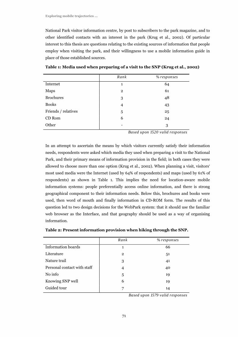
Exploring mobile trajectories …
71
National Park visitor information centre, by post to subscribers to the park magazine, and to
other identified contacts with an interest in the park (Krug et al., 2002). Of particular
interest to this thesis are questions relating to the existing sources of information that people
employ when visiting the park, and their willingness to use a mobile information guide in
place of those established sources.
Table 1: Media used when preparing of a visit to the SNP (Krug et al., 2002)
Rank % responses
Internet 1 64
Maps 2 61
Brochures 3 48
Books 4 43
Friends / relatives 5 25
CD Rom 6 24
Other - 3
Based upon 1520 valid responses
In an attempt to ascertain the means by which visitors currently satisfy their information
needs, respondents were asked which media they used when preparing a visit to the National
Park, and their primary means of information provision in the field; in both cases they were
allowed to choose more than one option (Krug et al., 2002). When planning a visit, visitors‘
most used media were the Internet (used by 64% of respondents) and maps (used by 61% of
respondents) as shown in Table 1. This implies the need for location-aware mobile
information systems: people preferentially access online information, and there is strong
geographical component to their information needs. Below this, brochures and books were
used, then word of mouth and finally information in CD-ROM form. The results of this
question led to two design decisions for the WebPark system: that it should use the familiar
web browser as the Interface, and that geography should be used as a way of organising
information.
Table 2: Present information provision when hiking through the SNP.
Rank % responses
Information boards 1 66
Literature 2 51
Nature trail 3 41
Personal contact with staff 4 40
No info 5 19
Knowing SNP well 6 19
Guided tour 7 14
Based upon 1579 valid responses

Exploring mobile trajectories …
72
When respondents were asked how they accessed information when in the Park, two thirds
used the information boards located in the field (see Table 2). This suggests that visitors
display an interest in information that is relevant to specific locations, and informed another
WebPark design decision, that the system should attempt to provide tools to allow the user to
retrieve information that is geographically relevant. People also relied on literature, nature
trails set up the Park and contact with park staff, suggesting that people prefer authoritative
sources of information (Krug et al., 2002).
Figure 13: Intention to use a mobile information system
Derived from 1597 responses to the WebPark user needs questionnaire (Krug et al., 2002)
0 10 20 30 40
No
Yes: for safety
Yes: withoutrestraint
Difficult to imagine
Other / nostatement
percent responses
Users were asked whether they would use such a system in the field; at this point in the
development cycle, no system had been developed hence the respondents had only
descriptions of how such a system might work. 37% replied with a straight “no”, suggesting
user scepticism could act a barrier to take up of mobile information systems. 44% replied
“yes”, although 24% of these would only use it as a safety feature (see Figure 13). The
remainder either did not reply, or would not express a preference since they could not
imagine such a system, suggesting that the novelty of a system may itself act as a barrier to
take-up.
3.3.3 Visitor shadowing
The second study undertaken to assess user needs comprised two visitor shadowing
exercises. In these exercises, visitors were accompanied on their trip by a member of the
WebPark team who recorded the questions they raised and problems they experienced. They
acted as a “human LBS”, recording and responding to queries, but not prompting the visitor

Exploring mobile trajectories …
73
for information. The intention was to assess mobile information needs and anticipate
potential scenarios of use of the system (Krug et al., 2002).
During the two user shadowing exercises, a total of 90 questions were recorded, of which 53
had some spatial reference related to the question. Of the 53 questions with a spatial
reference, 15 were related to navigation (eg “Where is the trail leading to Munt La Schera”,
“Where are we?”) or landscape (eg “Is this the Lake of Livigno?”). Of the remaining questions
with a spatial reference, 9 were related to park fauna (eg “Are there any marmots here?”), 12
to flora (eg “At what elevation is the timberline? Will we pass it on our way?”), and 8 to the
geomorphology (eg “Is this a moraine?”) (Krug et al., 2002). In many the spatial component
of the query was implicit as the question referred to the current location (eg “... around here
… ”), a visible location (eg “Which mountain is … ”) or a future location on the route (eg
“Will we pass …”). A full list of the 53 questions with a spatial reference can be found in
Appendix 1.
This implication that roughly 60% of queries have a spatial component is an interesting
result that is at odds with existing literature in this area which suggests that only about 20%
of queries have a spatial component (Sanderson and Kohler, 2004, Spink et al., 2002). There
are key differences between this particular user needs study and those in literature: this
study was conducted in an outdoor environment; the participants were mobile unlike those
in the literature; and user needs were recorded from comments and questions made by the
participant, rather formulating queries that were submitted to, and logged by, an Internet
search engine. The limited size of this user needs study means that care must be taken in
interpreting results, however one interpretation is that the discrepancy with the literature
could be due to mobile and outdoor individuals being more likely to have a spatial
component to their query, since their information needs are more likely to be influenced by
their surroundings. An alternative interpretation is that static users of Internet search
engines are as likely to have a spatial component to their information needs, but they do not
include a toponym or spatial relation in the query having learned from experience that this
spatial component is poorly handled by search engines (Sanderson and Kohler, 2004).
It was clear from this study that the information needs of mobile individuals frequently
contained a geographic component, that many queries would be meaningless without this
geographic context, and that the majority of such queries could not be satisfied by existing
information systems. The results of this study led to contemplation about the geographic
filters that could be applied to increase the relevance of retrieved information. It was clear
that users of mobile information systems engage with their surroundings, which provide a
dynamic backdrop likely to prompt questions, far more than their static counterparts whose
backdrop will be a more familiar predictable location, such as a workplace or the home (Krug
et al., 2002).

Exploring mobile trajectories …
74
3.4 Geographic filters for information retrieval
The following sections propose various geographic filters that attempt to increase the
relevance of the information retrieved by users of mobile information systems: this area of
work is closely related to the concept of geographic relevance (Raper et al., 2002). These
measures are represented as surfaces or geographic features that define regions of space that
are relevant for an individual, at some time, based upon some quantifiable geographic
criterion. Various assumptions are made about how information can be processed to be
made more relevant to the geographic context of the user. The first is spatial proximity,
where the closer an information source is to an individual, the more relevant it is. The
concept of spatial proximity can be represented with a (spatial) buffer around a point
location, a bounding box, or by generating a spatial proximity surface which can not only
define a region in space that is relevant, but differentiate within that space, based upon
distance from the user’s position or some other location. A more sophisticated assumption is
that of temporal proximity: regions that can be reached in a shorter period of time are more
relevant than those that are temporally distant. This concept can be defined by time
geography concepts such as potential path areas, and derived surfaces such as accessibility
surfaces. Another related assumption is that information that coincides with an individual’s
likely future locations is more relevant than that located in places they are unlikely to visit.
This can be modelled using speed-heading prediction surfaces, that provide an estimate of
the likelihood of an individual visiting different locations, based upon their recent spatial
behaviour. Other measures of geographic relevance are also suggested but not implemented
including those based upon visibility, making the assumption that people’s information
needs are inspired by what they see around them.
3.4.1 Spatial proximity
Perhaps the simplest and most intuitive measure to consider when attempting to define
geographic relevance is spatial proximity (Laurini and Thompson, 1992a): the key
assumption here is that locations that are closer in space to some feature, are more relevant
than those that are distant. This relates closely to what has been defined as the first law of
Geography, “everything is related to everything else, but near things are more closely related
than distant things” (Tobler, 1970). Different measures of spatial proximity can be defined
with distinct characteristics.
Buffer
A simple and familiar filter for defining a region of space representing an individual’s
geographic context is a buffer, which can be described by a circle of radius r, centred on the
location of an individual at a specific time (see Figure 14a). This buffer can be used within the
field of geographic information retrieval to retrieve all features within a specified distance of
an individual. The spatial buffer is a Boolean representation, where the region inside the

Exploring mobile trajectories …
75
circle is considered to be relevant, and the region outside the circle, not relevant. By
employing this Boolean approach it is not possible to distinguish between results that fall
within the circle; all that can be said is that these results are relevant, not how relevant. The
radius of the circle must be defined accord to some criterion and rules must be defined to
specify how areal features qualify for inclusion in a search. Some geographic search engines
allow people to define this sharp cut-off distance for themselves, for example “search within
500 metres of present location” (WebPark, 2005). A more sophisticated approach is to define
the cut-off automatically, using some criterion related to the user’s behaviour, such as the
present speed.
The minimum bounding rectangle (MBR) is similar to the spatial buffer in that a Boolean
region of space is defined that is deemed to be geographically relevant to a particular point in
space, however for a MBR the region is defined by a specified width and height, rather than a
circle of fixed radius r. An artefact of using a MBR is that two points that are the same
distance from the target location may be classified differently (one relevant, one not).
Nevertheless, the bounding box is frequently used as a heuristic within GIS and for
geographic information retrieval, since candidate features can be assessed to see whether
they are within the bounds very quickly, often prior to a more sophisticated and time
consuming procedure (Jones, 1997).
Spatial proximity surface
Buffers and MBRs both define Boolean regions centred on a point. It is also possible to
define a regular grid of cells (a raster) where values vary across the grid based upon distance
from some focal point, such as the centre: such a raster can be referred to as a spatial
proximity surface (see Figure 14b). This raster grid can also have a cut-off, defined by the
range where it is assumed that further increases in distance will have no further influence
over the values, ie beyond that point, all information is considered to be not relevant
(Burrough and McDonnell, 1998). This distance-weighting requires some decay function to
be applied. A Boolean spatial buffer assumes that no decay has been applied, and all
locations closer than the cut-off distance have the same value (see Figure 15a). Longley et al
(2005) describe three distance decay functions: linear distance decay, negative power
distance decay and negative exponential distance decay (Figure 15b - Figure 15d). Linear
decay is a less extreme decay function, where values on the surface are calculated according
to a linear relationship from the highest at the centre, to zero at and beyond the cut-off
(Figure 15b). The negative power distance decay function can provide a more extreme peak at
the centre of the surface, decaying faster to low values (Figure 15c); the size of the central
peak and rate of decay can be configured by manipulating the exponent, where higher
exponents provide a more extreme peak and faster decay. The negative exponential distance
decay function acts in a similar way to the power function, and can provide a more extreme
peak and faster decay than the linear function (see Figure 15d).

Exploring mobile trajectories …
76
Figure 14: Spatial proximity surfaces
a: Spatial buffer - Boolean surface defined by a circle of radius r, centred on a point
b: Spatial proximity surface - graded surface, with higher values (shown in lighter hues) closer to the centre
c: Offset spatial proximity surface - graded surface, with higher values (shown in lighter hues) closer to a specified distance from the centre
Data collected by David Mountain, Jun 2004 Images produced using the spatial history explorer.

Exploring mobile trajectories …
77
Distance decay functions - from Longley et al (2005)
Equation 1: Linear distance decay
Equation 2: Negative power distance decay
Equation 3: Negative exponential distance decay
W = a – bd W = d-b W = exp(-bd)
Figure 15: Distance decay functions: adapted from Longley et al (2005).
a: No decay b: Linear distance decay
no decay
00
distance
wei
ghtin
g
linear decay
00
distancew
eigh
ting
c: Negative power distance decay d: Negative exponential distance decay
negative power decay
00
distance
wei
ghtin
g
exponential decay
00
distance
wei
ghtin
g
e: Offset linear distance decay
linear decay (offset)
00
distance
wei
ghtin
g

Exploring mobile trajectories …
78
An alternative to the assumption that locations closer to the centre of the circle receive a
higher weighting that those elsewhere within the surface, is to choose some offset distance, at
which the maximum values are found (see Figure 15e). This creates a torus or donut shape;
values increase from a minimum at the centre of the surface to a maximum at the offset
distance, then decrease again to a minimum at the cut-off distance (see Figure 14c). The
same distance decay functions can be applied, for example offset linear distance decay
functions. This surface could be useful for predicting the future locations of moving point
objects when we have some idea of the distance that they are likely to cover, but are unsure
about in which direction they may travel. The spatial proximity surfaces can be normalised
(Sarle, 2002), where each cell value is divided by the mean cell value. Following
normalisation, the mean cell value is 1, with values below 1 reflecting more locations further
from the target, and values greater than 1, close locations.
3.4.2 Time Geography and temporal proximity
“The past is the key to the present” (Longley et al., 2005)
As discussed in the literature review, the emergence of time geography had a profound effect
upon notions of accessibility in the 1970s, placing emphasis upon modelling the behaviour of
individuals rather than groups of people (Hagerstrand, 1973). This approach has offered
considerable insight into the constraints faced in personal accessibility in terms of physical
capabilities, availability (of individuals and services) and authority restrictions. Implemented
models, however, have often made unrealistic simplifying assumptions such as ease of
movement in all directions (Lenntorp, 1976), since they have lacked fine-resolution spatio-
temporal data describing the behaviour of individuals, relying instead on travel diaries
(Kwan, 2000) . The visual representation of time geography concepts has traditionally been a
laborious process often undertaken by a dedicated graphics unit over a period of hours or
days; the final images were intended to communicate ideas to a mass audience, rather than
for exploration of the model or data itself.
Two key technological advancements have allowed time geography concepts to be
implemented in an interactive environment. The first is the increased processing speed and
memory of modern computers (Raymond, 2000), permitting the interactive analysis of large
volumes of quantitative data. The second is the availability of handheld GPS receivers that
can record the mobile trajectories at a much finer spatio-temporal resolution than travel
diaries (see section 3.1). This section describes how time geography techniques have been
implemented in an interactive environment, following this the concept of temporal proximity
will be explained, and how this may represent the geographic context of a mobile individual
in certain circumstances.

Exploring mobile trajectories …
79
The space-time path
Figure 16: Space-time path created interactively in the spatial history explorer
The image below shows a space-time path created interactively using the spatial history explorer software. The black points show the parent dataset from which the space-time path was extracted: one month’s spatial behaviour recorded in central London. The coloured points show the path; the green point represents the start of the path, yellow line shows the path itself and the red point represents the end of the path.
Data collected by David Mountain, Aug - Sep 2002 Images produced using the spatial history explorer.
As described in the Literature review (section 2.2), one of the most fundamental time
geography concepts is that of the space-time path (Miller, 1991) also known as the life path
(Hagerstrand, 1973) or mobile trajectory (Smyth, 2000). Temporal subsets of this complete
path can reveal a moving point object’s spatial behaviour over a week, a day or some other
temporally bounded period. In this section, the conventions will be adopted of using the term
‘mobile trajectory’ to refer to the parent data set, and ‘space-time path’ to refer to temporally
bounded subsets. An interactive approach to the space-time path has been implemented in
the spatial history explorer (SHE) software, where given a temporal duration (or time
budget) and origin (a spatial point location), the corresponding space-time path is rendered
in multiple views that can represent spatial, temporal and attribute dimensions (see Figure
16). The time budget of the space-time path must be specified in advance. The origin point
can be defined by clicking in a panel in SHE and selecting the nearest point in the parent set.
The nearest point may be defined by a spatial, temporal or attribute metric depending upon
the panel in which the click occurred.
The potential path area (PPA) or temporal proximity surface
Any one space-time path reveals the previous behaviour of a single moving point object over
a specific period of time. It is possible to aggregate a number of space-time paths, all of which
came close to the same spatial origin, to reveal the region of space that is accessible for a
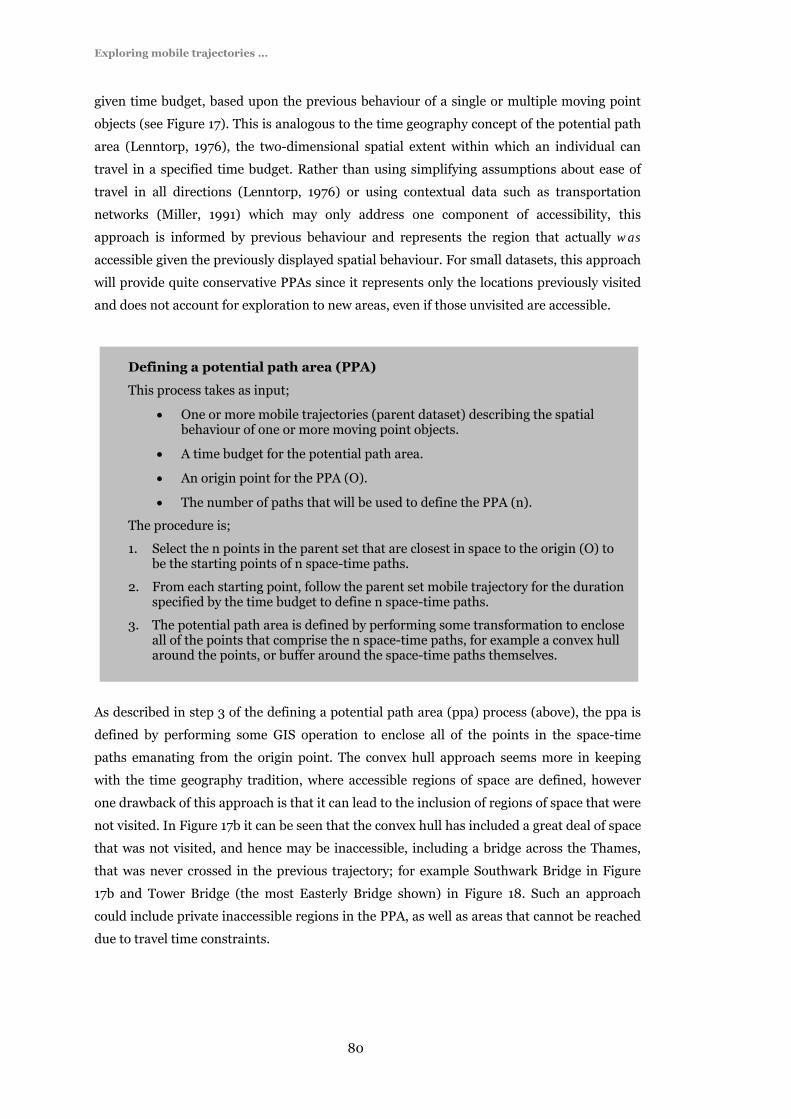
Exploring mobile trajectories …
80
given time budget, based upon the previous behaviour of a single or multiple moving point
objects (see Figure 17). This is analogous to the time geography concept of the potential path
area (Lenntorp, 1976), the two-dimensional spatial extent within which an individual can
travel in a specified time budget. Rather than using simplifying assumptions about ease of
travel in all directions (Lenntorp, 1976) or using contextual data such as transportation
networks (Miller, 1991) which may only address one component of accessibility, this
approach is informed by previous behaviour and represents the region that actually was
accessible given the previously displayed spatial behaviour. For small datasets, this approach
will provide quite conservative PPAs since it represents only the locations previously visited
and does not account for exploration to new areas, even if those unvisited are accessible.
As described in step 3 of the defining a potential path area (ppa) process (above), the ppa is
defined by performing some GIS operation to enclose all of the points in the space-time
paths emanating from the origin point. The convex hull approach seems more in keeping
with the time geography tradition, where accessible regions of space are defined, however
one drawback of this approach is that it can lead to the inclusion of regions of space that were
not visited. In Figure 17b it can be seen that the convex hull has included a great deal of space
that was not visited, and hence may be inaccessible, including a bridge across the Thames,
that was never crossed in the previous trajectory; for example Southwark Bridge in Figure
17b and Tower Bridge (the most Easterly Bridge shown) in Figure 18. Such an approach
could include private inaccessible regions in the PPA, as well as areas that cannot be reached
due to travel time constraints.
Defining a potential path area (PPA)
This process takes as input;
• One or more mobile trajectories (parent dataset) describing the spatial behaviour of one or more moving point objects.
• A time budget for the potential path area.
• An origin point for the PPA (O).
• The number of paths that will be used to define the PPA (n).
The procedure is;
1. Select the n points in the parent set that are closest in space to the origin (O) to be the starting points of n space-time paths.
2. From each starting point, follow the parent set mobile trajectory for the duration specified by the time budget to define n space-time paths.
3. The potential path area is defined by performing some transformation to enclose all of the points that comprise the n space-time paths, for example a convex hull around the points, or buffer around the space-time paths themselves.

Exploring mobile trajectories …
81
Figure 17: Using space-time paths to define a potential path area:
In a, four space-time paths (shown in yellow with green and red endpoints) have been extracted from the parent mobile trajectory (shown as transparent black points), using four origin points close to a user defined starting point; they demonstrate that in the past, movement to the North, South, East and West has been displayed from this location. In b, 12 space-time paths have been enclosed using a convex hull, to define a potential path area representing the region of space accessible within 10 minutes.
a: Four space-time paths: time budget = 10 minutes
b: Potential path area: time budget = 10 minutes
Data collected by David Mountain, Aug - Sep 2002 Images produced using the spatial history explorer.
An alternative approach is to use a buffer around the space-time paths themselves, which
results in a region that is more spatially constrained, and with less opportunity for overlap

Exploring mobile trajectories …
82
into regions that were not visited. An appropriate buffer distance should be selected: for GPS
data the reported accuracy since the ending of deliberate signal degradation due to selective
availability (The White House: Office of the Press Secretary, 2000) is between 10 to 25
metres, depending upon the type of receiver and environmental conditions (Enge and Misra,
1999, Porcino, 2001). Such a small buffer distance may be appropriate if there is sufficient
data density, however for smaller datasets, larger buffer distances may be required to prevent
the potential path areas being unrealistically small. In the study, a buffer distance of 250
metres has been applied around the space-time paths. The resulting regions of space form
accessibility corridors, and are generally more precise than the convex hull approach.
The potential path area is a crisply delineated, homogenous area that defines what region of
space is accessible for a given time budget, no distinction is made about how accessible one
region of the ppa is relative to another. Such information, however, is stored implicitly within
mobile trajectories and the next two sections will consider ways of extracting and
representing accessibility as a phenomenon with indeterminate boundaries. The potential
path area acts as temporal proximity surface, analogous to the spatial proximity surfaces
described in section 3.4.1. Whereas a spatial proximity surface can define the region of space
within x metres of the present location, the potential path area can define the region of space
accessible within t minutes of the present location, based upon previously displayed
behaviour.

Exploring mobile trajectories …
83
Figure 18: Alternative approaches to bounding the sections of the mobile
trajectory, accessible with a given time budget
Based upon the previous behaviour of a single individual in Central London during Dec 2003
a: bounding points with a convex hull b: bounding points with a 250 metre spatial buffer
The hull is shown as a transparent orange region with a red boundary, generated around a series of origin points (in green). The yellow paths show the sections of the mobile trajectory that had been traversed from the origin points, within 5 minutes.
The buffer is shown as a transparent orange region, generated around a series of origin points (in green). The yellow paths show the sections of the track log that had been traversed from the origin points, within 5 minutes. The intensity of the orange colour represents the density of space-time paths, so darker orange regions were visited many times, lighter orange visited infrequently.
Data collected by Pete Boyd, Dec 2003 Images produced using the spatial history explorer.
Isochrone surfaces
An isochrone surface can be derived from a series of potential path areas all of which have
the same origin but different time budgets. It is a graded surface comprised of a series of
concentric polygons, centred on an origin point (see Figure 19). Travel time increases as you
cross a boundary between two polygons, moving away from the origin. This introduces
heterogeneity into the concept of accessibility; some locations within the surface are
temporally closer to the origin than others, which is not the case for locations within the
potential path area.

Exploring mobile trajectories …
84
Figure 19: Isochrones surfaces: regions accessible from Blackfriars bridge in 15
minutes or less.
The spatial behaviour of one individual, recorded over a one month duration and clipped to Central London, has been analysed to generate the isochones shown in the right panel. Each successive red polygon, heading out from the central red point, shows the area accessible within an additional 3 minutes. The largest enclosing red polygon, the 5th isochrones, therefore represents the region accessible within 15 minutes. It can be seen, that for this particular individual, speed of travel is faster in a North-South direction than in an East-West direction.
Data collected by David Mountain, Aug - Sep 2002 Images produced using the spatial history explorer.
Accessibility surfaces
An accessibility surface is a raster grid where each cell represents the travel time from a
spatial location (the origin). Representing accessibility in this way avoids the inclusion of
inaccessible areas and homogeneity that is associated with potential path areas and
isochrones surfaces. Raster modelling does not place the constraint on accessibility that time
travel can only increase with distance from the surface origin as unlike the isochrone surface,
it does not reply upon concentric polygons.
There are many parameters that can influence this surface. The size of cells in the output grid
represents the spatial resolution of the surface. Using a larger grid cell size reduces the
processing time associated with calculating the surface, however the associated decrease in
spatial resolution may lead different components of the transportation network, with very

Exploring mobile trajectories …
85
different characteristics, falling into the same set of cells (for example, a railway line running
alongside a canal). When calculating the travel time to each cell in the raster, a distance
weighted mean can be used, or an alternative is to use the minimum travel time value of
those points that fall within the search buffer since people are often interested in how fast
they can travel to different locations. Accessibility surfaces are similar to the approach of
Forer, who implemented time geography concepts using a raster model of space (see section
2.2).
Temporal Proximity Summary
For this study, the potential path area will be used to model temporal proximity since it is
considered to be the most appropriate representation and conceptually closest to the original
work of the time geography school. The justification for adopting this representation, above
all those described is that, unlike the space-time path, it represents the region of space (areal
representation as described in section 2.1.2 of the Literature Review) associated with a
particular time budget. Furthermore, it is an object (vector) representation as opposed to a
field (raster) representation (this distinction is also described in section 2.1.2). As described
in the Literature Review (section 2.2), the original time geographers applied object
representations of accessible areas and field representations, such as the accessible surface
described above, have accounted for only a small percentage of this research.
3.4.3 Speed-heading predictions
Of the existing approaches for predicting the future locations of moving point objects, many
have been criticised for assuming that those objects move according to simple linear
functions and for failing to capture the complexity of motion patterns (Tao et al., 2004). Of
the methods available for predicting the future location of moving point objects, the idea of
using speed and either turning angle or heading from correlated random walk analysis
(Byers, 2001) was identified as a useful approach, particularly since this has been applied for
modelling the future locations of moving point objects (often animals), based upon their
previous behaviour. As discussed in section 2.3.1 implementations of correlated random
walks frequently lack the volume of data required to generate valid statistical distributions
for input parameters to the model. The spatial and temporal resolution of the data repository
collected as part of this study is sufficiently fine to permit the calculation of statistical
distributions for parameters such as speed, heading, turning angle and step size. The
following sections describe the influence of different parameters when making predictions
about future behaviour, and how the ideas from correlated random walk analysis were
adapted to use a moving point object’s mobile trajectory to create a prediction surface.
Whilst this form of prediction is closely related to correlated random walk analysis, it
considers only heading and not turning angle when predicting future locations. The

Exploring mobile trajectories …
86
justification for this is that we wish to predict the destination of the moving object, rather
than construct a model of recent movement that could describe the motion pattern seen
when travelling to that destination. When making a prediction based upon turning angle, the
initial starting direction used in correlated random walk analysis can be crucial, and may
result in a good model of motion pattern that heads initially in an arbitrary direction. By
using heading, the model of motion is less effective, but the prediction will continue on the
heading described by previous behaviour, and be less affected by very recent deviations away
from the overall direction of movement. For this reason, these predictions will be referred to
as speed-heading predictions, to indicate that they are based upon an extrapolation from the
current location given values to describe speed and heading, and to differentiate this
approach from correlated random walks. This is a new approach to this problem.
Several new terms will be used when discussing predictions. The two- (or three-)
dimensional spatial point location from which the prediction is being made is referred to as
the prediction origin, and the time at which a prediction is being made, the prediction start
time (t) the prediction spatial origin and start time are typically defined by the most recent
point in a mobile trajectory, or the time and place where a mobile user has an information
need and performs a search for geographically relevant information. One issue to consider is
what period into the past should be considered, when predicting a moving object’s future
location. In this discussion, the period of time elapsed since the start time for which a
prediction will be made is referred to as the prediction period: this is the “20 minutes”
parameter predicting where an object will be “20 minutes from now”, hence a long-term
prediction will use a greater value for prediction period than a short-term prediction. In the
context of testing a prediction, a verification point or destination point refers to the actual
known location of the moving point object at the time for which the prediction is made. The
term recent behaviour is used to define the spatial behaviour of a moving point object (as
described by its mobile trajectory) from some specified period of time in the past until the
prediction start time. The principle behind the application of correlated walk analysis in this
context is therefore to predict the future location of some moving point object, from the
analysis of its recent spatial behaviour.
Point predictions
Wolfson and Yin (2003) provide a definition for predicting the future location of a moving
point object, based upon linear extrapolation from a known location along a straight line at a
constant speed. Given these assumptions, a single, future point location can be calculated
using the arithmetic mean of speed and the circular mean of heading for a moving point
object’s recent behaviour. An example of this is shown in Figure 20.
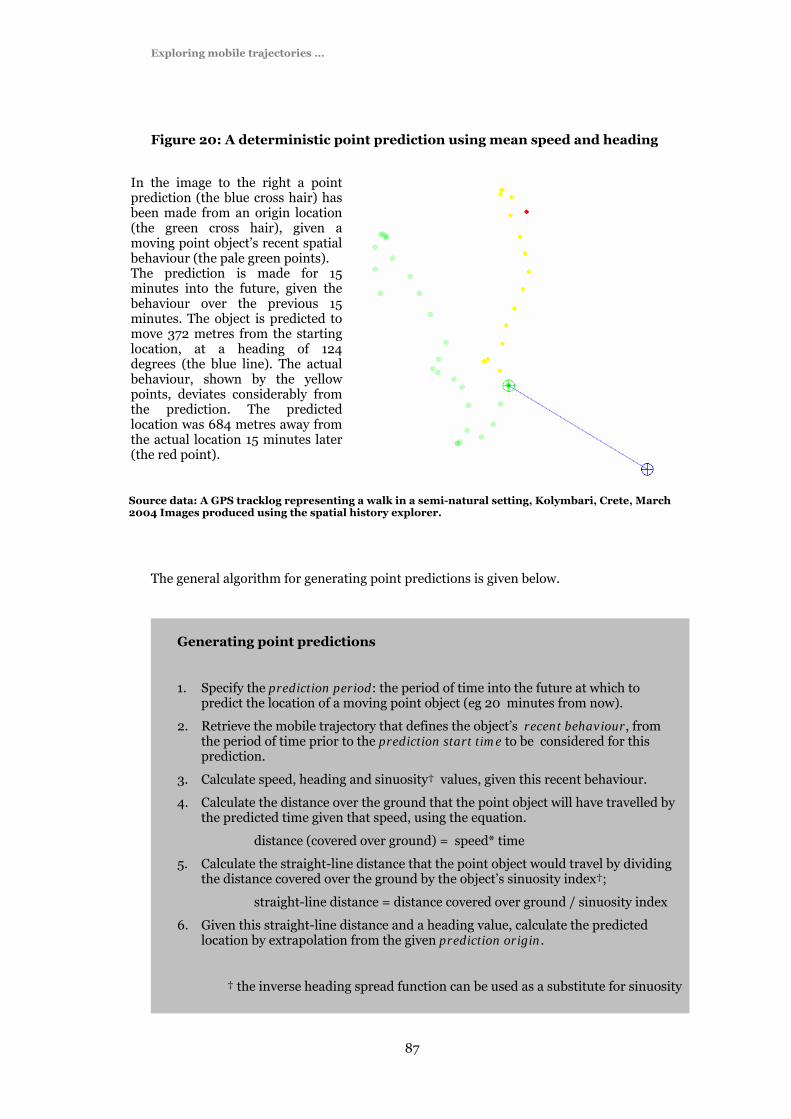
Exploring mobile trajectories …
87
Figure 20: A deterministic point prediction using mean speed and heading
The general algorithm for generating point predictions is given below.
Generating point predictions
1. Specify the prediction period: the period of time into the future at which to predict the location of a moving point object (eg 20 minutes from now).
2. Retrieve the mobile trajectory that defines the object’s recent behaviour, from the period of time prior to the prediction start time to be considered for this prediction.
3. Calculate speed, heading and sinuosity† values, given this recent behaviour.
4. Calculate the distance over the ground that the point object will have travelled by the predicted time given that speed, using the equation.
distance (covered over ground) = speed* time
5. Calculate the straight-line distance that the point object would travel by dividing the distance covered over the ground by the object’s sinuosity index†;
straight-line distance = distance covered over ground / sinuosity index
6. Given this straight-line distance and a heading value, calculate the predicted location by extrapolation from the given prediction origin.
† the inverse heading spread function can be used as a substitute for sinuosity
In the image to the right a point prediction (the blue cross hair) has been made from an origin location (the green cross hair), given a moving point object’s recent spatial behaviour (the pale green points). The prediction is made for 15 minutes into the future, given the behaviour over the previous 15 minutes. The object is predicted to move 372 metres from the starting location, at a heading of 124 degrees (the blue line). The actual behaviour, shown by the yellow points, deviates considerably from the prediction. The predicted location was 684 metres away from the actual location 15 minutes later (the red point).
Source data: A GPS tracklog representing a walk in a semi-natural setting, Kolymbari, Crete, March 2004 Images produced using the spatial history explorer.
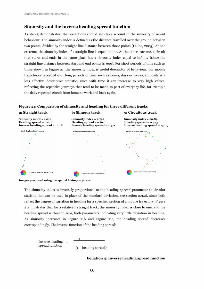
Exploring mobile trajectories …
88
Sinuosity and the inverse heading spread function
As step 5 demonstrates, the predictions should also take account of the sinuosity of recent
behaviour. The sinuosity index is defined as the distance travelled over the ground between
two points, divided by the straight line distance between those points (Laube, 2005). At one
extreme, the sinuosity index of a straight line is equal to one. At the other extreme, a circuit
that starts and ends in the same place has a sinuosity index equal to infinity (since the
straight line distance between start and end points is zero). For short periods of time such as
those shown in Figure 21, the sinuosity index is useful descriptor of behaviour. For mobile
trajectories recorded over long periods of time such as hours, days or weeks, sinuosity is a
less effective descriptive statistic, since with time it can increase to very high values,
reflecting the repetitive journeys that tend to be made as part of everyday life, for example
the daily repeated circuit from home to work and back again.
Figure 21: Comparison of sinuosity and heading for three different tracks
a: Straight track b: Sinuous track c: Circuitous track Sinuosity index = 1.019 Heading spread = 0.018 Inverse heading spread = 1.018
Sinuosity index = 2.792 Heading spread = 0.611 Inverse heading spread = 2.571
Sinuosity index = 20.89 Heading spread = 0.923 Inverse heading spread = 13.09
Images produced using the spatial history explorer
The sinuosity index is inversely proportional to the heading spread parameter (a circular
statistic that can be used in place of the standard deviation, see section 2.3.2), since both
reflect the degree of variation in heading for a specified section of a mobile trajectory. Figure
21a illustrates that for a relatively straight track, the sinuosity index is close to one, and the
heading spread is close to zero, both parameters indicating very little deviation in heading.
As sinuosity increases in Figure 21b and Figure 21c, the heading spread decreases
correspondingly. The inverse function of the heading spread:
Equation 4: Inverse heading spread function
Inverse heading spread function
(1 – heading spread)
1 =
Exploring mobile trajectories …
89
provides a statistic that is similar in magnitude to the sinuosity. It is this parameter that is
used in step 5 of the calculating point prediction process, since whilst sinuosity can only give
a single figure to describe the sinuosity for all spatial behaviour that is defined as recent, the
inverse spread function can be weighted by temporal distance to allow the most recent
behaviour to have a greater influence than that in the more distant past (see Equation 1 -
Equation 3 and Figure 15), a process described in more detail in the following section.
Recent behaviour and time weighted statistics
The problem posed by the increasing sinuosity index raises a wider question of what period
of time should be used to define recent behaviour. Wolfson and Yin (2003) provide a
definition for predicting the future location of a moving point object, based upon linear
extrapolation from a known location along a straight line at a constant speed. Given these
assumptions, a single, future point location can be calculated using the arithmetic mean of
speed and the circular mean of heading for a moving point object’s recent behaviour. An
example of this is shown in Figure 20. In Figure 20, recent is taken to mean all spatial
behaviour displayed over the previous 15 minutes, hence the values for sinuosity (or inverse
heading spread function), mean speed and mean heading used for the prediction are based
upon the previous 15 minutes of the mobile trajectory: the cut-off is sharp between points
that are included in analysis (<15 mins), and those that are not (>15 mins).
Given the assumption that more recent behaviour is more indicative of what an individual
will do in the immediate future, than behaviour in the more distant past, it is appropriate to
calculate a weighted mean for speed and heading in step 3 of the algorithm to generate point
predictions, where greater significance is given to more recent points. This is similar to the
inverse distance-weighted approach described for spatial proximity surfaces, but instead of
using spatial separation to define distance, points are weighted according to their separation
in time from the most recent point in the set. The separation in time for each point in the set
is given by the number of seconds (or some other temporal interval) by which it precedes the
prediction start time. These values are then rescaled in a linear fashion from zero to one so
that the earliest point has the largest ‘distance’ separation (1) and the most recent point the
least (0).
Given these rescaled separation values, different inverse-distance weighted functions can be
applied to provide a weight for each point in the set. Linear distance decay is illustrated in
Figure 15b and is characterised by giving relatively high weightings to the earlier points in
the set. Negative power and negative exponential distance decay give relatively higher
weightings to more recent points in the set, and the rate of decay can be controlled by the
distance-decay parameter, b (see Equation 1, Equation 2 and Equation 3 on p77).

Exploring mobile trajectories …
90
Given these distance decay functions, weighted statistics can be calculated for speed and
heading that are more influenced by the most recent behaviour. The weighted mean is
calculated using the equation;
Equation 5: Weighted mean
Where ∑wx is the sum of all weighted values and ∑w is the sum of all weights (Shaw and
Wheeler, 1985). When calculating speed, the value of x is the speed value itself in metres per
second or some other appropriate measurement unit. In the case of heading, the circular
angle value (in degrees, radians or some other circular measure) cannot be used directly. The
mean for heading is calculated by plotting each point on the unit circle according to its
heading value and calculating the centroid of the points which will always fall on or within
the unit circle (described in section 2.3.2).
The weighted standard deviation for speed can be calculated in a similar way;
Equation 6: Weighted standard deviation
For heading, the weighted spread is used instead of standard deviation (Brunsdon and
Charlton, 2003, Cox, in press, Fisher, 1993, Mardia and Jupp, 1999). Since the spread value
can be weighted, the inverse heading spread function can also be weighted to reflect the
sinuosity of more recent behaviour, and not simply the sinuosity index of the entire mobile
trajectory.
Stochastic predictions
Regardless of whether the mean is weighted or not, a single point prediction is of limited use
for defining the geographic footprint of a query based upon where a moving point object is
likely to be in the future in the context of mobile information retrieval. Retrieved search
results may be ranked by distance from the prediction, but this is not a significant
improvement upon the simple proximity searches that are the current paradigm in location-
based services, such as the “Find nearest” service from UK mobile phone operator Orange
(Orange, 2005) which operates on strict linear distance. Applying a deterministic approach
(Burrough, 1998) that uses only the mean of speed and heading fails to consider the
distribution of the data set that comprises recent behaviour; the prediction will always be in
the same place given the same recent behaviour. One criticism of existing approaches to
Weighted mean
∑wx
∑w =
Weighted standard deviation
∑w(x – xMean)
∑w
= √ ( )

Exploring mobile trajectories …
91
prediction has been the simplification associated with linear extrapolation (Tao et al., 2004).
Such approaches take no account of the complexity or degree of variation in the previous
trajectory used to calculate the speed and heading values.
Figure 22: Frequency distribution of speed for 9870 GPS points collected in the
UK in March and April 2004
Whilst for this dataset, the distribution displays some bimodal characteristics, with peaks at 10 and 27 metres per second suggesting two different primary means of transport, the Normal distribution still provides a reasonable fit for this data set using a mean = 15.2, standard deviation = 11.3.
Knowing the standard deviation of speed and heading, and assuming a Normal distribution
(or a wrapped Normal distribution for heading), a random element can be introduced to
derive a series of non identical point predictions, based upon the same previous behaviour.
Analysis of nearly 10,000 data points collected over one month (Mar – Apr 2004) suggests
that the motion attributes associated with mobile trajectory appear to be Normally
distributed (see Figure 22). You may expect to see bi- or multi-modal distributions for larger
volumes of this kind which reflect the presence of many different examples of activity within
the same data set; for example a peak associated with walking behaviour, another associated
with driving and so on. Such a trend is evident to a certain extent in Figure 22. It is likely that
the Normal distribution will be a better model when a single activity is represented in the
data (for example, just driving behaviour), than when multiple activities are represented.
Using this stochastic approach, the process to calculate the speed and heading values in step
2 of the generating point predictions algorithm is a little more complex. First a pseudo-
random number between zero and one is generated; this number is taken to represent an
area under the Normal curve, between -∞ and some upper zed score. Transforming the
standard (z) score to a value for the data set (x) is a basic statistical technique and can be
achieved by using the equation;

Exploring mobile trajectories …
92
Equation 7: Transforming zed scores
given that the mean (µ) and standard deviation (σ) of the dataset are known. Applying this
technique allows a prediction of a future location to be made, which incorporates a random
element based upon the distribution of speed and heading.
The predictions described above for both the deterministic and stochastic approaches are
modelled as single steps from the origin location to the final predicted destination. This is a
valid heuristic if the intermediate behaviour is not required, and the distance travelled takes
account of the sinuosity of the dataset (step 5 of generating point predictions algorithm). It is
also possible to calculate a multistep prediction by calculating a series of predictions for the
duration of the prediction.
The speed-heading prediction surface
By adopting this stochastic approach (Burrough, 1998) a Monte Carlo simulation
(Openshaw, 1998b) can be run where a number of predictions are made over a range of
locations, which may be more versatile than the single deterministic point prediction for two
main reasons. First, placing a bounding box around the predictions produces an two-
dimensional area footprint, which moves from the simple proximity spatial relation to that of
containment; candidate result features can be examined to see if they fall within the
prediction surface bounding box, not just by measuring their distance from some point
location. Second, creating a point density surface of the point predictions gives variation
within the bounding box; cells with high values represent locations the moving point object is
likely to be, cells with low values are less likely to be visited, based upon the moving point
object’s recent behaviour.
x = (z * σ) + µ

Exploring mobile trajectories …
93
Figure 23: Generating a surface based upon a series of stochastic predictions.
The torus shape in the prediction (b) is determined by the previous behaviour, shown by the pale green points. Previous movement is very sinuous and meanders to the East, however speed is quite consistent suggesting that the object is unlikely to remain in the same location. The surface performs well when compared to the object’s known future location.
a: Multiple point predictions 250 point predictions (the blue crosshairs) of the future location of a moving point object 15 minutes into the future, are shown for the same origin location (the green cross hair). The predictions are based upon the object’s behaviour over the previous 15 minutes.
b: Speed-heading prediction surface A point density surface (720 metres width) generated for the 250 prediction points in a. The surface values have been rescaled to between zero (unlikely to be visited - lighter) and one (most likely to be visited - dark). The red cross hair shows the point object’s actual location 15 minutes later, where the surface has a value of 0.36.
Source data: A GPS tracklog representing a walk in a semi-natural setting, Kolymbari, Crete, March 2004 Images produced using the spatial history explorer.
Differentiation within surfaces
The value of each cell in the grid surface is point density, measured in points per unit area.
By normalising (Sarle, 2002) the cell value by the mean cell value, a relative point density
value is given, where the mean value of all cells is equal to one.
Relative point density = cell point density / mean surface point density
Equation 8: Relative point density
These relative point density cell values offer an effective way of assessing which regions of
the grid are more likely to be visited (greater than one) and which are less likely to be visited
(less than one). The area outside the grid has a value of zero, since point density outside the

Exploring mobile trajectories …
94
grid is zero. Relative point density is a dimensionless measure, since it is the ratio of point
density at a particular location, to the average point density over a region. Such a grid can be
used to rank candidate query results, as discussed later in section 3.6.
Instant vs interval predictions
As discussed in section 2.1.3, there is a distinction between events that occur at some exact
instant in time, and intervals which have a duration in time (Langran, 1992). It is possible to
predict future locations at an instant in time, or for an interval with a specified temporal
duration. Both may be useful in the context for mobile information retrieval. In the first
instance, you may have a need for a specific service at a known time in the future, for
example, a restaurant to stop at a time that is agreeable for lunch. Interval predictions can be
applied to retrieve features that are likely to be passed in the future, for example, an
ornithologist walking in a National Park, wishing to know the locations of rare birds’ habitat
that they are likely to pass over the course of the next hour.
When generating a prediction surface that describes the likely position of a moving point
object at an instant in the future, the prediction period is fixed to the specified value for all
the point predictions that are used to generate the prediction surface. This will tend to
produce prediction surfaces that are smaller and more focussed and, for longer prediction
periods, that are further from the prediction origin. When generating surfaces for an interval,
the prediction period should be varied, through the introduction of a random element, from
0 to twice the prediction period. This tends to produce surfaces that resemble a torch beam
shining out from the prediction origin in the direction of movement as defined by the recent
behaviour.
3.5 Prediction surfaces
In the previous sections, various approaches to defining the geographic context of a mobile
individual have been proposed. In the context of spatial and mobile information retrieval,
these can be seen as geographic filters performing a post query filter, allowing a further
ranking of candidate results identified as being relevant on the subject level (Saracevic,
1996b). The aim of these geographic filters is to include a measure of situational relevance
(Saracevic, 1996b), based upon an individual’s location and previously displayed spatial
behaviour. One key assumption to be investigated is that for mobile individuals, the future
location - as opposed to current location - could be used as an alternative means of assessing
geographic relevance, or as the focus for retrieving location-based information (Brimicombe
and Li, 2004). There are various contexts in which this may true. First, mobile individuals
requesting specific services (such as foods, shops, accommodation, fuel, leisure facilities) or
location-based information (with no assumption that this information must relate to a

Exploring mobile trajectories …
95
specific service) are likely to be more interested in those that are ahead of them than those
around or behind them. This is demonstrated effectively by people requesting current travel
information from a moving car on a motorway. The travel information closest in space may
be behind them, hence no longer relevant to them, or else on surrounding roads, that are
actually quite distant from them in terms of the distance over the transport network and
travel time. In this context, a geographic filter gives a higher ranking to information whose
geographic footprint is related to places that are ahead of the car than that based solely on
spatial proximity. In another context, visitors to an outdoor recreational area such as a
National Park may be interested in the flora and fauna that they are likely to encounter
during a walk. Once the walker has passed a point on a walk, they are less likely to wish to
turn back on themselves to visit it again. Again information related to the areas they are
likely to visit can have greater situational relevance than the past or present location.
Of the three approaches described in section 3.4 (spatial proximity, temporal proximity,
speed-heading predictions), all could be applied to predict the future location of a moving
point object.
• Spatial proximity prediction surfaces: Any of the spatial proximity surfaces
described in section 3.4.1 could be used for prediction, making the assumption that
the current position, or some offset from it, is a good estimate of future location.
• Temporal proximity prediction surfaces: The potential path area described in
section 3.4.2 could be used as temporal proximity surface, predicting future
locations on the assumption that future movement will be subject to the same
authority and capability constraints as that displayed in the past.
• Speed-heading prediction surfaces: These can be used for prediction, on the
basis that immediate future spatial behaviour will be correlated to recent behaviour.
Given these three approaches to prediction we need unbiased evaluation criteria to compare
the performance of these different approaches. We can assume that the each prediction will
be a surface, which may be homogenous within its boundaries (eg spatial buffer, potential
path area), or display internal variation where higher values represent the locations that the
moving point object is more likely to go (eg spatial proximity surface, speed-heading
prediction surface). Each prediction will have an origin (usually the last known position of
the moving point object), a start time (t), and a prediction period. Given these common
characteristics of prediction surfaces, the following section describes the development of
criteria that could evaluate, in an unbiased manner, the effectiveness of different approaches
to prediction.

Exploring mobile trajectories …
96
3.5.1 Evaluation criteria for prediction surfaces
According to Stockwell and Peters (1999) ”there are two main ways of evaluating predictive
modelling systems”: demonstrating validity on a theoretical basis, or the use of “empirical
trials and comparisons with alternative systems”. The mobile trajectories used in this study
are represented by a series of time-stamped point locations, so the future sections of those
mobile trajectories can be used to find the actual destination of a moving point object at the
predicted time, and these verification points used to evaluate the effectiveness of any given
prediction (see Figure 24). The datasets collected as part of this research were recorded at a
sufficiently fine spatio-temporal resolution to allow an empirical approach to be adopted.
This design was intended to test these prediction surfaces against observed reality – the
actual spatial behaviour as displayed by individuals - as opposed to simulations based upon
assumptions about how individuals move over space through time, which will always display
some element of bias and hence the results of which will always be more open to
interpretation. Various approaches to prediction will be tested, and compared using the same
evaluation criteria.
Figure 24: Evaluation criteria to compare the effectiveness of three individual prediction surfaces, illustrated using spatial buffers.
a: 10km buffer predicting location in 10mins (verification point falls outside buffer)
b: 20km buffer predicting location in 10mins (verification point falls inside buffer)
c: 40km buffer predicting location in 10mins (verification point falls inside buffer)
The buffer is shown as a yellow region with a red boundary, generated around an origin point (in green) and compared to a verification point (in red). Extent of images is about 70km width from Plymouth (SW) to Exeter (NE) in the UK. Data collected by David Mountain, 9 Jun 2004 Images produced using the spatial history explorer.
Prediction surface effectiveness criteria
For 10km spatial buffer Verification value = 0 (outside buffer) Surface area = pi * 100002 = 314,159,265 m2
Prediction surface effectiveness = Verification value / surface area = 0
For 20km spatial buffer Verification value = 1 (inside buffer) Surface area = pi * 200002 = 1,256,637,061m2 Prediction surface effectiveness = Verification value / surface area = 8.0*10-10
For 40km spatial buffer Verification value = 1 (inside buffer) Surface area = pi * 400002 = 5,026,548,245 m2
Prediction surface effectiveness = Verification value / surface area = 2.0*10-10

Exploring mobile trajectories …
97
In some situations no verification points may be available, for example when the GPS
receiver loses a positional fix, or when the end of a trajectory is reached. When no
verification points are available, the prediction cannot be evaluated and is excluded from
analysis. The sampling frequency of the positioning system means that there may not always
be a verification point recorded at the exact required instant that coincides with the
prediction time. For this study, the point temporally closest to the prediction time is used for
verification, as long as it occurs within one minute of the predicted time. If there is no
verification point within one minute of the required time, the prediction is again excluded
from analysis. For predictions that estimate the location of a moving point object for an
instant in time (eg exactly 10 minutes from now), a single verification point is used. When
making a prediction over an interval in time (eg during the next 10 minutes), a series of
verification points can be used. For ease of description, the following discussion describes the
case for predictions made for an instant in time, however it should be noted that these
evaluation criteria can be extended to consider predictions made over an interval in time.
Tests that attempt to assess the effectiveness of predictions of future locations of moving
points objects typically measure the distance between the predicted destination, and the
actual destination at the predicted time. Sharma et al (2005) use the term prediction
accuracy, to describe the absolute distance (in two-dimensional space) between the
predicted and actual point location. Vasquez and Fraichard (2004) use the estimation error
to describe the performance of their predictions: this is the measure of the distance between
a predicted and actual trajectory, hence is a measure of dissimilarity. While these definitions
of prediction error and accuracy are useful, they cannot be directly applied to the case where
a surface, representing a region of space, has been used to predict a point location, describing
the future location of a moving object. When considering individual predictions of this kind,
two factors are important: the location of the verification point relative to the prediction
surface, and the area of the prediction surface.
An independent evaluative test is required to compare the effectiveness of different
prediction surfaces in an unbiased manner. For effective prediction surfaces, the verification
point will fall within the surface, and – if the surface is heterogeneous – coincide with cells
that have relatively high values. An added criterion is that these surfaces should be small in
spatial extent, reflecting the fact that they are precise, not “scattergun” predictions that cover
a large area and are therefore much more likely to coincide with the verification point. An
additional requirement is that our evaluation should be able to compare not just individual
prediction surfaces, generated for a single point in time, but how well one approach
performs in comparison to another in different situations. Hence the evaluation criteria
should consider the performance of a particular approach over a period of time where many
prediction surfaces are generated in an iterative manner, one for each point in a mobile
trajectory representing spatial behaviour in some situation.

Exploring mobile trajectories …
98
Given the need to ensure that the evaluation testing is fair and unbiased, the evaluation
criteria themselves have been subjected to a series of tests to assess how they perform in
different situations. It was decided to test the evaluation criteria by using buffers of different
radii (described in section 3.4.1) to assess the characteristics of different candidate
evaluation criteria when comparing individual surfaces, and to see how they perform when
applied iteratively for an entire trajectory. Spatial buffers were chosen as a control since they
are a basic and well-understood transformation within GIS, and since this type of geographic
filter is widely used in LBS when retrieving location-based information.
Normalisation of prediction surfaces
As described in section 3.4.1, buffers are Boolean surfaces, where the area inside the cutoff
can be given a value of one, and the area outside a value of zero. The same principle applies
to the potential path areas (temporal proximity surfaces) described in section 3.4.2. As
mentioned in sections 3.4.1 and 3.4.3, spatial proximity surfaces and speed-heading surfaces
can be normalised (Sarle, 2002), to ensure that the mean value within the surface is one. In
this way we can ensure that there is no systematic variation in the surface values between
approaches, since the mean value within all prediction surfaces is equal to one.
3.5.2 Evaluation of individual prediction surfaces
We will first consider evaluation criteria that allow the characteristics of individual
prediction surfaces to be described, and their effectiveness compared, before moving on to
describe evaluation criteria that describe characteristics and account for the consistency of
an approach in a particular situation, over a series of predictions.
Verification value
The first criterion that can be used for evaluation is the verification value: this is the value of
the surface at the point that coincides with the verification point (the actual destination at
the predicted time). For all surfaces, this value is zero outside the surface bounds. For
Boolean surfaces (buffers, and potential path areas) this verification value will be one if the
point falls within the surface bounds. For continuous surfaces (spatial proximity surfaces and
speed-heading surfaces) the verification value will be the value of the cell that coincides with
the verification point. This value can tell us, therefore, whether the surface coincided with the
actual destination at all, in the first instance, and in the second instance - for continuous
surfaces - whether it coincided with high or low values. Large surfaces will perform well
according to this criterion, since they are more likely to coincide with the actual destination.
Since we do not wish to reward scattergun predictions, that are large in extent, we must also
take account of the surface area.

Exploring mobile trajectories …
99
Figure 25: Verification value
The green point is the prediction origin and the red the verification point. The verification value is given by the value of the cell in which the verification point falls. Where the verification point falls outside the grid, a value of zero is recorded.
Verification value > 1 Verification value ≈ 1
Verification value < 1 Verification value = 0
Images produced using the spatial history explorer
Surface area
This is a measure of the spatial extent of the surface. An assumption is that effective
prediction surfaces will generally be smaller in extent, hence this criterion provides an
opportunity to assess how that extent varies for different approaches in different scenarios.

Exploring mobile trajectories …
100
Prediction surface effectiveness
It is assumed that for effective prediction surfaces:
The verification point will be higher than for ineffective ones
The surface area will be smaller than for ineffective ones.
Hence our measure of the effectiveness for individual prediction surfaces can be given by:
Equation 9: Prediction surface effectiveness
This measure appears upon first consideration to offer a complete approach to assessing the
effectiveness of prediction surfaces, and also the effectiveness of a particular approach over
the course of an entire trajectory. Surfaces where the verification point coincides with high
grid values, and where the overall extent of the surface is small, will perform well according
to this criterion. The units of measurement are m-2, which are the same as the relative point
density (per metre2) measure used for the speed-heading predictions.
When this evaluation criterion is applied to a spatial buffer prediction, for a point on a
mobile trajectory collected in Devon (see Figure 24), the characteristics of this evaluation
criterion can be assessed. For a 10km buffer, the verification point falls outside of the buffer
(a value of zero), so the prediction surface effectiveness will also be zero. For a 20km buffer,
the verification point falls inside the buffer, so the prediction surface effectiveness measure
is 8.0*10-10. For a 40km buffer, the verification point again falls inside the buffer, and the
final prediction surface effectiveness measure is 2.0*10-10. This demonstrates that the
prediction surface effectiveness of the 40km buffer is just ¼ that of the 20km, due to their
relative surface areas. The 10km has a value of zero, as it did not coincide with the
verification point. This approach appears to give a reasonable approach to comparing the
effectiveness of individual surfaces, since it is sensitive to both the value at the verification
point and the surface area.
3.5.3 Evaluation of a prediction approach
Measures are also required that can describe the characteristics and assess the performance
of one prediction approach, where multiple predictions are generated for all the points in a
Prediction surface effectiveness = verification value
surface area

Exploring mobile trajectories …
101
particular mobile trajectory, to get a longer-term view of how it performs in a particular
situation. This is a measure of the consistency of an approach, how effective it was in a
particular scenario over a period of time, as opposed to for a single prediction. Various
potential evaluation criteria were considered. The average (mean or median) verification
value and surface area can be used for description, but for a comparison of effectiveness,
other measures are required.
Success rate
The success rate is a common concept that describes the effectiveness of predictions,
forecasts, and systems generally (Vasquez and Fraichard, 2004), for a series of predictions,
given by the ratio of successes to total attempts made. Xu and Wolfson (2003) use a similar
measure that they refer to as precision - the ratio of correct predictions to the total number of
predictions - to evaluate the effectiveness of their approach. For this study the success rate
will be defined as;
Equation 10: Success rate
A success occurs when the prediction surface overlaps with the verification point, regardless
of where on the surface the point falls. A failure occurs when the point falls outside the
prediction surface. The total number of attempts is given by the total of successes and
failures. A success rate of zero indicates that the surface never coincided with the actual
destination. A success rate of one indicates that it always coincides with the destination. This
measure is closely related to the verification value for comparing individual surfaces. For
Boolean surfaces, the mean verification value will be the same as the success rate (since both
are the ratio of successes to total attempts). It also shares the key drawback of the verification
value, that larger surfaces tend to perform better, since it cannot differentiate between those
appropriately sized surfaces that consistently just coincide with the destination, and those
scattergun approaches that achieve high success rates because the surfaces cover a very large
spatial extent. An approach is required that can reflect the effectiveness of surfaces (in terms
of having a small spatial extent, and having high verification values) and the consistency of
an approach.
n attempts
Success rate =
n successes

Exploring mobile trajectories …
102
Average prediction surface effectiveness
The prediction surface effectiveness (PSE) can assess the effectiveness of a single prediction,
and the success rate can assess the consistency of an approach over a series of prediction
surfaces. Whilst these are both useful measures, a single evaluation criterion is desirable that
can compare how two approaches perform in the same situation. This has led to the
definition of the average prediction surface effectiveness. Two measures of central tendency
are described below, and their strengths and weaknesses contrasted.
Mean prediction surface effectiveness
The first measure that was investigated was to use the mean value over the series of
prediction surfaces: the prediction surface effectiveness is calculated for each prediction in a
particular situation, and the mean used to describe the effectiveness of that approach in that
particular situation. Despite the attractiveness of this method, testing conducted with buffers
was found give counter-intuitive results. A small number of very effective surfaces (buffers
with small surface areas), could skew the overall mean so that very inconsistent approaches
with low success rates appeared to perform well. This can be best illustrated with an
example. This evaluation criterion was tested for a driving journey from St Austell in
Cornwall to St Albans in Hertfordshire (see section 4.1.1 for a full description); several buffer
sizes were tried to see which were effective in predicting location 10 minutes ahead. The
overall result, when applying this evaluation criterion, was that very small spatial buffers that
hardly ever coincided with the verification point performed very well, due to their very small
surface area. However buffers of a size that frequently just coincided with the verification
point, that one would intuitively consider to be the most effective for predicting future
location, performed less well. Of all buffers tested, the most effective according to this
evaluation criterion was the 1000m buffer, however this only coincided with the verification
point 1% of the time over the duration of the journey. The 15km buffer, which coincided with
the verification point 71% of the time, and 20km buffer (coincided 99% of the time) on the
other hand, achieved lower mean prediction surface effectiveness scores.
“Even a stopped clock tells the right time twice a day”
from the film, “Withnail and I” (Robinson, 1987)
These approaches, that achieved high mean prediction surface effectiveness values from the
performance of a small proportion of predictions were labelled “stopped clocks”, since
although they were almost always poor (failing to coincide with the verification point), very
occasionally the approach achieved extremely high prediction surface effectiveness scores. A
stopped clock, by way of analogy, usually tells the wrong time, but twice a day is exactly
correct. A clock that is a few minutes slow, by contrast, always tells approximately the right
time – and most would argue more useful to the wearer - but is never so precisely correct.
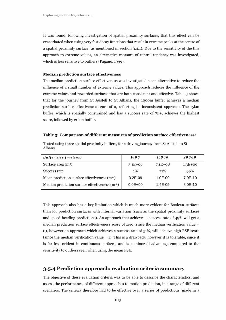
Exploring mobile trajectories …
103
It was found, following investigation of spatial proximity surfaces, that this effect can be
exacerbated when using very fast decay functions that result in extreme peaks at the centre of
a spatial proximity surface (as mentioned in section 3.4.1). Due to the sensitivity of the this
approach to extreme values, an alternative measure of central tendency was investigated,
which is less sensitive to outliers (Pagano, 1999).
Median prediction surface effectiveness
The median prediction surface effectiveness was investigated as an alternative to reduce the
influence of a small number of extreme values. This approach reduces the influence of the
extreme values and rewarded surfaces that are both consistent and effective. Table 3 shows
that for the journey from St Austell to St Albans, the 1000m buffer achieves a median
prediction surface effectiveness score of 0, reflecting its inconsistent approach. The 15km
buffer, which is spatially constrained and has a success rate of 71%, achieves the highest
score, followed by 20km buffer.
Table 3: Comparison of different measures of prediction surface effectiveness:
Tested using three spatial proximity buffers, for a driving journey from St Austell to St Albans. Buffer size (metres) 1000 15000 20000
Surface area (m2) 3.1E+06 7.1E+08 1.3E+09
Success rate 1% 71% 99%
Mean prediction surface effectiveness (m-2) 3.2E-09 1.0E-09 7.9E-10
Median prediction surface effectiveness (m-2) 0.0E+00 1.4E-09 8.0E-10
This approach also has a key limitation which is much more evident for Boolean surfaces
than for prediction surfaces with internal variation (such as the spatial proximity surfaces
and speed-heading predictions). An approach that achieves a success rate of 49% will get a
median prediction surface effectiveness score of zero (since the median verification value =
0), however an approach which achieves a success rate of 51%, will achieve high PSE score
(since the median verification value = 1). This is a drawback, however it is tolerable, since it
is far less evident in continuous surfaces, and is a minor disadvantage compared to the
sensitivity to outliers seen when using the mean PSE.
3.5.4 Prediction approach: evaluation criteria summary
The objective of these evaluation criteria was to be able to describe the characteristics, and
assess the performance, of different approaches to motion prediction, in a range of different
scenarios. The criteria therefore had to be effective over a series of predictions, made in a

Exploring mobile trajectories …
104
particular scenario. It was decided that a combination of evaluation criteria would be useful
in describing the characteristics of prediction surfaces: these are described below. The
median values were used, to reduce the influence of the “stopped clocks” described above.
Median verification value: An assessment of the degree to which the surface coincided
with the actual destination, and whether it coincided with high values on the surface, or low
ones. It is useful as a descriptive statistic, but rewards large surfaces, hence should not be
used as a measure of effectiveness.
Median surface area: The spatial extent of the prediction surface with the assumption
that smaller prediction surfaces are more effective than larger ones.
Median prediction surface effectiveness: A measure of the effectiveness and
consistency of an approach. This value was used to compare the effectiveness of different
approaches.
Success rate: A measure of the consistency of an approach, which tended to reward larger
surfaces. It was found to be useful as a descriptive statistic.
3.5.5 Implementation of prediction surface tests
Within the interactive geoVisualization software application, the spatial history explorer, the
procedures to generate the prediction surfaces described above, and perform the evaluative
tests to assess their performance, have been implemented. Different approaches to
prediction can be applied, including spatial proximity, temporal proximity, and speed-
heading predictions. The tests are described in more detail in the Results section (section 4.1)
however they are based upon the criteria described above, and are performed by proceeding
through a given mobile trajectory in an iterative manner, generating a single prediction
surface for each point in the set, then generating aggregate results for overall performance
over the entire set. Input parameters, such as the period of time to predict into the future, the
period of time to use as “recent behaviour”, and the temporal weighting to be applied, can be
modified for each test. Results include the quantitative evaluation criteria described above,
and qualitative visual output, in the form of an animated film, where each frame of the film
shows the prediction surface generated for a single point in the dataset. Although these
animations, by their very nature, cannot be included in a paper thesis, they communicate
very useful feedback about the conditions in which particular approaches and configurations
perform well or poorly. This information has in turn informed the design process. Selected
animations are available on the CD ROM that accompanies this thesis, and can also be
downloaded from the associated website at http://www.soi.city.ac.uk/~dmm/phd
(Mountain, 2005a).

Exploring mobile trajectories …
105
3.6 Sorting results using geographic filters
Having developed an approach to generate surfaces of values between zero and one that
represents, in some way, the geographic context of a query - such a speed-heading prediction
surface, spatial proximity surface, or temporal proximity surface - results that match the
query at the subject level can also be ranked according to the degree to which they are
relevant geographically. This is an attempt to quantify the situational relevance (Saracevic,
1996a) based upon specific geographic criteria. As part of the WebPark mobile information
system described in section 3.3, a speed-heading prediction filter was implemented that
allowed users of the system to search based upon where they were likely to be in the future:
the tools was referred to as the “search ahead” filter.
In the WebPark implementation, the geographic footprints associated with location-based
information could have point, line or area geometry: these information sources were referred
to as features of interest (FOIs), as opposed to points of interest (POIs), to reflect this. A
process has also been defined that allows a geographic relevance score to be assigned to these
features of interest.
Equation 11 demonstrates that there are two distinct aspects to the score. First, the mean
value of the cells in the geographic filter that intersect with the feature. Second, the degree to
which the feature is contained within the geographic filter, the aim being to improve the
ranking of results that area relevant locally. This is a technique that has been adapted from
Calculating a geographic relevance score for features of interest
This process takes as input;
• a feature with a spatial footprint that represents a candidate query result,
• a geographic filter: a surface of value, scaled between zero and one, that defines in some way the geographic characteristics of the query.
The procedure is;
1. Intersect the feature footprint and geographic filter,
2. Calculate the mean value of the grid cells within the intersect,
3. Weight the mean value given in 2. by the degree to which the feature’s spatial footprint is contained within the geographic filter.
This is summarised in the equation below;
Equation 11: Geographic relevance score
Geographic relevance
score =
Mean cell value in feature-surface
intersect Feature size
Intersect size *

Exploring mobile trajectories …
106
existing measures of spatial similarity (Larson and Frontiera, 2004). The principle behind
this approach is that features with large spatial extents tend to less be relevant in any one
place than features with small, well-defined spatial extents.
3.6.1 Point features
Points represent the simplest case since they have no spatial extent. The first step is to
intersect features with the relevance grid, points will either fall entirely inside the grid and
should be retained, or entirely outside and should be disregarded. The geographic relevance
score is given by the value of the grid cell within which the point feature falls. There is no
need to apply the final weighting since in effect, the feature size and intersect size are the
same.
Figure 26: Geographic relevance scores for point features
In the example shown to the left, five red point features represent five candidate results. The greyscale surface is a rescaled grid that represents the spatial extent of the query, where dark cells are more relevant (close to one) and light cells are less relevant (close to zero). The three red points to the South and South East of the surface can be dismissed since they do not intersect with the grid. Of the two points that fall within the grid, the more central one falls within a cell with a higher value, hence has higher geographic relevance score than the point feature to the West.
3.6.2 Line features
For candidate results represented by a line feature, for example roads, rivers, walking routes
or boundaries, the line should again be intersected with the geographic filter grid and the
mean cell value along the intersection calculated. The mean value of the intersected cells
should then be weighted by the ratio of the length of the intersection to the total length of the
line feature.

Exploring mobile trajectories …
107
3.6.3 Area features
First an intersect operation should be performed for the feature and the geographic filter
grid. If there is no overlap then the result can be disregarded as not geographically relevant
based upon the current criteria. If there is overlap, then the mean value of the cells in the
intersection should be calculated. In the case where the feature is wholly contained within
the geographic filter, this mean cell value is the result. Where the overlap is only partial, it is
weighted by the ratio of the intersect area to the feature area.
Figure 27: Geographic relevance scores for area features
a: Relevance surface (greyscale) and area feature (blue)
b: Intersection (shaded grey scale) and original feature (broken line)
In the above example the feature (a lake shown in blue in the left panel) is intersected with a
surface that defines the geographic footprint of a query; in this case the surface is a
prediction of the places that the individual making the query is likely to be in 30 minutes
time (shown in grey scale in the left panel). The values of cells vary from 0 in light grey (least
likely to be visited) to 1 in black (most likely to be visited); the width of the grid is 3250
metres. The resulting intersection (shown in greyscale to the right) has a mean cell value of
0.097 (≈10%). This should be weighted by the ratio of the intersection area (254679m2) to
the feature area (351233m2). The final geographic relevance of the lake, based upon a
prediction of where the user is likely to be in 30 minutes time, is

Exploring mobile trajectories …
108
Geographic relevance score = mean cell value within intersect * (intersect area/lake
area)
Geographic relevance score = 0.097 * (254679 / 351233)
Geographic relevance score = 0.0703346
Therefore, the geographic relevance score for the lake is 7%
Bounding box heuristic
Figure 28: The bounding box heuristic
Calculating the geographic relevance scores for feature with area and line geometry was
found to be very computationally demanding. A bounding box heuristic was adopted, to
reduce the complexity of the procedure and allow results to be returned in real-time. A
bounding box was place over the features and this box intersected with the query footprint.
Rather than taking the mean of all of the points in the surface, the value of the cell at the
centroid of the intersection was used, and this multiplied by the ratio of the intersection
extent to the feature extent. This offers can approach of scaling this approach to allow large
volumes of results to be ranked according to geographic context.
3.6.4 Geographic Information ranking implementation
These approaches to sorting geographic information based upon geographic filters as
described above have been implemented as part of the WebPark platform, described in
section 3.3. In an implementation developed for the Swiss National Park, three spatial filters
were available. These were:
Search whole park: where no spatial filter was applied;
Areal extent of geographic footprint of feature
Surface representing geographic footprint of query
Value at centre
of intersection

Exploring mobile trajectories …
109
Search around me: where a spatial proximity filter was applied;
Search ahead: where a speed-heading prediction based upon recently observed
behaviour was applied.
The user controlled which filter they wished to apply at the query formulation stage by
selecting the desired filter using a radio button on a web page in browser on the mobile
device. The user could specify the semantic component of the query either by selecting
checkboxes associated with a list of pre-defined topics, or using a natural language search
interface. The interface to this location-based search tool is shown in Figure 29. The results
from user evaluation of these geographic filters are analysed in section 4.4.
Figure 29: Geographic filters implemented in the WebPark system
a: the selection of the filter at the query formulation stage.
b: ranking by the likelihood of an individual coinciding with the geographic footprint associated with each result.
Images generated using the WebPark platform, for a specific implementation in the Swiss National Park
3.7 Methodology Summary
This Methodology section first described the collection of data about the movement of
individuals, and the development of a geoVisualization tool – the spatial history explorer – to
analyse these mobile trajectories. Next a mobile platform and test best were described for a
mobile information retrieval application, built upon the WebPark architecture. The
development of geographic filters for information retrieval then described various
approaches to modelling individual accessibility, and detailed ways in which these concepts
can be applied to generate prediction surfaces of the likely future locations of an individual,

Exploring mobile trajectories …
110
based upon their previous behaviour. The definition of evaluation criteria for these
prediction surfaces were then described, and the implementation of procedures in the spatial
history explorer to generate predictions and evaluative their effectiveness for a larger
number of points. Finally, approaches that apply the surfaces to the task of retrieval
geographic information have been defined.
The next section (Results) will first describe various test scenarios, and test configurations,
before applying the evaluation criteria to both describe and assess the performance of
different approaches in different conditions.

Exploring mobile trajectories …
111
4 Results
Results Abstract
This section presents both quantitative results, related to the performance of prediction
surfaces according to the evaluation criteria described in section 3.5, and qualitative
results, based upon testing geographic filters for information retrieval in an outdoor
mobile computing environment as part of a major user evaluation study in the Swiss
National Park, in the Summer of 2004.
The chapter begins with quantitative evaluation, where three test scenarios are described
(walking, driving and daily migration), followed by a description of the systematic
variation in the temporal component of prediction, designed to compare short-term (10
minutes) and long-term (60 minutes) predictions into future. Next, three geographic
filters described in the methodology are introduced as prediction surfaces. The three
filters are spatial proximity, temporal proximity and speed-heading predictions. For each
approach, the prediction input parameters were varied in a systematic way to uncover the
impact of buffer size and distance decay functions (for spatial proximity prediction
surfaces), the ‘recent behaviour period’, temporal weighting and decay function (for
speed-heading prediction surfaces) and the time budget and enclosing function (for
temporal proximity prediction surfaces). Next, the results are presented and analysed to
describe, explain and contrast the characteristics of each prediction approach. This is
followed by a brief assessment of the suitability of each approach to the scenarios in
which it was tested.
Overall, predictions based upon temporal proximity are found to be more effective than
speed-heading predictions, which in turn out are more effective than predictions based
upon spatial proximity.
Finally, the chapter concludes with the results of the user evaluation study, which
suggests that users of mobile information retrieval tools found the implemented “search
ahead” filter useful, are receptive to the idea of other geographic filters, and benefit from
the use of personalised geographic information with a spatial and temporal component.

Exploring mobile trajectories …
112
4.1 Prediction testing framework
“It is difficult to make predictions, especially about the future"
Unattributed saying, from Wikipedia (2005), variously attributed to Confucius, Mark
Twain, Benjamin Disraeli, Albert Einstein, Sir George Bernard Shaw, Winston
Churchill, Niels Bohr, Cecil B. DeMille, Woody Allen, etc…
As discussed in section 2.4, there are a great many potential approaches for predicting the
future location of moving point objects, and more specifically people. A testing framework
has been devised that allows the characteristics of different approaches to be described, and
assess how each approach performs in different situations, when configuration parameters
are systematically varied. Three approaches to prediction are compared: speed-heading
prediction surfaces, spatial proximity prediction surfaces, and temporal proximity prediction
surfaces. Three different scenarios of human behaviour have been tested: walking, driving,
and a ‘daily migration’ scenario. Both short-term (10 minute) and long-term (60-minute)
predictions have been made for the walking and driving scenarios. Various configuration
parameters have been tested in a systematic and repeatable way, which are described for
each of the three approaches in the following sections. In all, 528 individual tests were run.
The results of all tests are included in tabular form in appendix 3, and graphical
representations of these figures are given within each section.
4.1.1 Behaviour scenarios
It is possible, to some degree, to distinguish classes of human spatial behaviour - such as
sitting, walking, or moving in a vehicle such as a car, bus, train or plane – where each class of
behaviour has distinct characteristics (Golledge and Stimson, 1997). Movement on foot tends
to be relatively unconstrained in the direction of travel, but more constrained in terms of the
distance that can be covered, due to the slow maximum speed of movement. Movement by
mechanised transport tends to be less constrained in terms of speed, but more constrained
by transportation networks which can restrict the freedom to change direction (Dykes and
Mountain, 2003). For these tests three scenarios were tested: a walking scenario, a driving
scenario, and the ‘daily migration’ pattern described by the round trip from home to work
and back. All datasets were derived from GPS data collected as described in section 3.1.
For each scenario, a section of mobile trajectory has been extracted that represents a
particular class of spatial behaviour. As part of the analysis, prediction surfaces will be
generated – and their characteristics described and effectiveness assessed - for each of the n
points that comprise this section of the trajectory; this set of points will be referred to as the

Exploring mobile trajectories …
113
mobile trajectory testing set or the testing set. The testing set for each scenario was
extracted from a longer parent mobile trajectory, which describes the spatial behaviour of
that individual prior and subsequent to the test set. This parent trajectory can provide
verification points, for predictions close to the end of the test trajectory, and can contribute
to the recent behaviour, particularly for points closer to the start of the test trajectory, and
tests that use a long time period to define recent behaviour. The use of the parent set in this
way avoids the ‘edge effects’ apparent at the start of the test, when no or limited previous
behaviour would otherwise be available from which to determine the speed and heading of
predictions, and at the end of the set, when no verification points would be available to assess
the effectiveness of the predictions.
Walking scenario
For the walking scenario, a section of mobile trajectory was extracted that described the
ascent and descent of a mountain (Helvellyn), starting and finishing in Patterdale in the
English Lake District (see Figure 30). The walking scenario test trajectory itself consisted of
226 unique, time-stamped point locations. The walking route took about 4hrs to complete
and was characterised by a slow average speed (2.8 kmph) and highly sinuous behaviour.
The route describes a steep profile ascending 900 metres in height from Patterdale to
Helvellyn, returning by an alternative route to describe a circuit that resembles a figure of
eight. The slope was generally steep and the terrain often rough underfoot, particularly near
the summit. The downhill sections of the mobile trajectory were generally faster than those
ascending and at the summit (see Figure 31). The parent mobile trajectory displays driving
and walking behaviour, as described in Figure 32.

Exploring mobile trajectories …
114
Figure 30: Walking scenario: Mobile trajectory test set
The track log shows a circuitous route around Helvellyn (South West Corner) starting from Patterdale (in the North East). The ascent begins on paths common to ascent and descent before diverging to take a more Northerly course closer to Birkhouse Moor, then heading South West over Grisedale Brow to ascend Helvellyn via Striding Edge. The return route completes the figure of eight, first descending North East via Swirral Edge, before crossing the ascending track at Grisedale Brow to take the more Southerly route before rejoining the path back into Patterdale.
Data collected by David Mountain, 9 Nov 2004, from 10:53 – 14:53 Image produced using the spatial history explorer.
Figure 31: Time vs elevation plot for Helvellyn walking behaviour
The plot below shows the time of day plotted against elevation (using the WGS84 vertical datum), for the track log displayed in Figure 30. The points are shaded using a sequential colour scheme from dark (slow) to light brown (fast) (Brewer, 2005). It can be seen that the slowest section of the route was at the summit, where the terrain is both steep and rough. Downhill and flat sections away from the summit are generally characterised by faster speeds; uphill sections on average show slow speeds. Note the unadjusted height values from the GPS, that describe the vertical height above the WGS84 ellipsoid, not height above sea level in the UK.
Image produced using the spatial history explorer.

Exploring mobile trajectories …
115
Figure 32: Walking scenario parent set
The testing set for the walking scenario was preceded by 2 days of walking in the Scottish Highlands, with travel by car between the walks. The 24 hours immediately preceding the test set is characterised by a walk in the Scottish Highlands the previous day, followed by a drive South to Settle in Yorkshire, an overnight stay, then a 1hr30 drive to Patterdale. Immediately after the test set, the parent set records a period of no movement (resting in a café), followed by a journey South by car. This parent set was used to compare predictions to the actual location at the predicted time and available of a source of ‘recent behaviour’ for speed-heading predictions.
Data collected by David Mountain, 06-10 Nov 2004. Image produced using the spatial history explorer.

Exploring mobile trajectories …
116
Driving scenario
The driving scenario describes a car journey from St Austell in Cornwall, to St Albans in
Hertfordshire, UK, via fast A-roads and motorways (see Figure 33). The journey was a
generally high speed event (mean 80kmph), with slower speeds on the more minor roads at
the start of the journey, and a number of stops for fuel and refreshment. The route is
relatively straight following a heading towards the East-North-East as indicated by both the
sinuosity index (1.16) and the inverse heading spread function (1.15) (Figure 34). The driving
scenario mobile trajectory test set consists of 195 unique, time-stamped point locations. The
parent set contains 4 days of predominantly driving behaviour, with some walking behaviour
displayed.
Figure 33: Driving scenario: Mobile trajectory test set
Car journey from St Austell (South West of the map) to St Albans (North East) driving along A-roads and motorways. Points are shaded by speed from relatively slow (dark brown) to fast (light brown).
Data collected by David Mountain, 9 Jun 2004, from 13:55 – 20:12 Image produced using the spatial history explorer.

Exploring mobile trajectories …
117
Figure 34: Driving scenario test set: characteristics of speed and heading
The mobile trajectory test set describing the car journey from St Austell to St Albans is characterised by generally high speed behaviour (mean 22 m/sec or 80 kmph). There is limited variation in heading, with travel generally heading towards the North East.
Data collected by David Mountain, 9 Jun 2004, from 13:55 – 20:12 Image produced using the spatial history explorer.
Figure 35: Driving scenario: Parent mobile trajectory
The parent set for the driving scenario included journeys by car from St Albans to Nottingham, then on to the South West in the preceding days. The previous 24 hours was characterised by a journey by car from Dartmoor to St Austell, an overnight stay, a short car journey in the morning, followed by the test set itself. The parent set ends at the same time as the test set, hence some of the later predictions in the test set could not be compared to the actual location at the predicted time.
Data collected by David Mountain, 9 Jun 2004, from 05 -09 Jun 2004 Image produced using the spatial history explorer.

Exploring mobile trajectories …
118
Daily migration scenario
Figure 36: “Daily migration” scenario: parent mobile trajectory The parent mobile trajectory for the daily migration scenario was collected over the duration of 5 weeks. It included walking behaviour, cycling, driving, and travel on buses, trains and the London underground. Most time was spent within Greater London, however journeys were also taken to the English Lake District, and Stoke-on-Trent in the Midlands.
a) The full parent set for the daily migration scenario - showing a concentration of behaviour around London, with trips to the North
b) The parent set for the daily migration scenario, zoomed in to Central London - the mobile trajectory representing the daily migration scenario is shown as a yellow space-time path.
c: Temporal distribution - the plot below shows absolute time on the x axis vs day of the week on the y axis. This shows that data was collected almost every day for 5 weeks, and that the majority of movement occurred at low speed (green colours), with infrequent high speed events.
Data collected by David Mountain, 16:56:13 20/08/2002 to 15:27:09 21/09/2002 Image produced using the spatial history explorer.

Exploring mobile trajectories …
119
The daily migration scenario test set consists of 35 points describing two journeys across
central London by bicycle: from home to work in the morning, and the return journey in the
evening (see Figure 36b). The parent mobile trajectory was collected by one individual
between 20 Aug and 21 Sept 2002, and includes movement on foot, by bicycle, by bus,
underground, train and car (see Figure 36a). This previously exhibited spatial behaviour was
available to the temporal proximity algorithm to predict where this individual was likely to
be in the future, based upon the area accessible to them in the past from that location.
4.1.2 Long-term and short-term predictions
In order to test the effectiveness of different approaches at making both long-term
predictions into the distant future, or a short-term predictions into the near future, two
prediction periods have been tested;
t + 10 minutes: to represent a short-term prediction
t + 60 minutes: to represent a long-term prediction
For the walking and driving scenarios, both short-term and long-term predictions have been
made. For the daily migration scenario, only short-term behaviour has been tested, since
sections of the mobile trajectory associated with the journey to work are themselves less than
one hour in duration.
4.1.3 Prediction configuration parameters
Three approaches to prediction were tested in all; speed-heading predictions, spatial
proximity prediction surfaces, and temporal proximity predictions surfaces. Each approach
has configuration parameters which have been varied systematically to assess their influence,
and to see which configurations are suited to which scenarios.
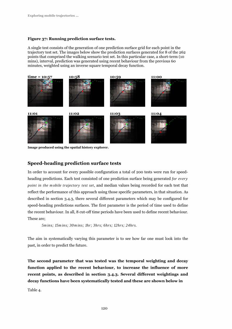
Exploring mobile trajectories …
120
Figure 37: Running prediction surface tests.
A single test consists of the generation of one prediction surface grid for each point in the trajectory test set. The images below show the prediction surfaces generated for 8 of the 262 points that comprised the walking scenario test set. In this particular case, a short-term (10 mins), interval, prediction was generated using recent behaviour from the previous 60 minutes, weighted using an inverse square temporal decay function.
time = 10:57 10:58 10:59 11:00
11:01 11:02 11:03 11:04
Image produced using the spatial history explorer.
Speed-heading prediction surface tests
In order to account for every possible configuration a total of 200 tests were run for speed-
heading predictions. Each test consisted of one prediction surface being generated for every
point in the mobile trajectory test set, and median values being recorded for each test that
reflect the performance of this approach using those specific parameters, in that situation. As
described in section 3.4.3, there several different parameters which may be configured for
speed-heading predictions surfaces. The first parameter is the period of time used to define
the recent behaviour. In all, 8 cut-off time periods have been used to define recent behaviour.
These are;
5mins; 15mins; 30mins; 1hr; 3hrs; 6hrs; 12hrs; 24hrs.
The aim in systematically varying this parameter is to see how far one must look into the
past, in order to predict the future.
The second parameter that was tested was the temporal weighting and decay
function applied to the recent behaviour, to increase the influence of more
recent points, as described in section 3.4.3. Several different weightings and
decay functions have been systematically tested and these are shown below in
Table 4.

Exploring mobile trajectories …
121
Table 4: Temporal weightings and decay functions
Weighting Decay
function
Description
None None All recent behaviour (up to the cut-off) has the same
influence
Temporal Linear Influence of less recent behaviour diminishes by a linear
inverse distance-decay function, up to a cut-off (see
Figure 15: Distance decay functions: adapted from
Longley et al (2005).Figure 15 and Equation 1).
Temporal Negative power Influence of less recent behaviour diminishes by a
negative power decay function, up to a cut-off, where
points cease to have an influence (see Figure 15 and
Equation 2). Temporal decay parameters that have been
tested are 1.5, 2, 3.
For the walking and driving scenarios, a total of 160 tests were run: this accounted for the 2
scenarios, 2 prediction periods, 5 decay functions for temporal decay, and 8 periods of recent
behaviour (see Table 5).
Table 5: Situations and configurable parameters for which the speed-heading
prediction surfaces were tested
Scenario N prediction
periods
N recent
behaviour
periods
N temporal
weightings /
decay
functions
N
configurations
tested
Walking 2 8 5 80
Driving 2 8 5 80
Daily migration 1 8 5 40
Total - - - 200
A further 40 tests were run for the daily migration, where short-term predictions were made,
for the 8 periods of recent behaviour, and 5 temporal weighting and decay functions.
Each prediction surface itself was generated as described in section 3.4.3 by generating 200
random point predictions (based on the distributions for speed and heading), and calculating

Exploring mobile trajectories …
122
the normalised point density for a grid of 32 columns width, placed over the point
predictions. The process of generating a series of prediction surfaces is described in Figure
37. After each test, four values recording the evaluation criteria described in section 3.5.4
were recorded: the median verification value; the median surface area; the median prediction
surface effectiveness; and the success rate.
Spatial proximity prediction surface tests
Whilst this surface was not designed explicitly as a prediction surface, it acts as a useful
control against which to compare the other approaches. The main assumption with this
surface is that where you are now provides a good prediction of where you are likely to be in
the future. In the absence of any further information, this is a reasonable heuristic to adopt
and can reduce a search space from the global (everywhere on earth), to the local (the
immediate vicinity of this individual).
In all, 318 tests were conducted for the spatial proximity prediction surfaces. The tests were
performed for 3 scenarios: walking, driving and daily migration. The first configuration
parameter for spatial proximity prediction surfaces that was systematically tested was the
buffer distance employed. For the walking and daily migration scenarios 11 buffer distances
were tested (distances are in metres);
100; 250; 500; 750; 1,000; 1,500; 2,000; 3,000; 5,000; 7,500; 10,000
For the driving scenario 10 buffer distances were tested;
250; 500; 1,000; 5,000; 10,000; 15,000; 25,000; 50,000; 100,000; 250,000.
It is worthy of note that these distances were selected with the scenario in mind - smaller
buffer distances for walking and commuting behaviour, greater distances for driving - in
order to avoid testing buffer sizes that are very unlikely to be effective, such as a 250km
buffer for short-term walking prediction. The effectiveness of this approach is highly
dependent upon buffer size, and without some information indicating an individual’s spatial
behaviour, such as current speed, wholly inappropriate buffer sizes could be used.
The second parameter that was tested was the distance weighting and decay function
applied. As described in the methodology, this has the effect of producing higher values
around some target point (or points), usually the prediction origin, decreasing as you move
away from the target. Six distance weighting and decay functions were tested: no weighting;
linear decay; linear-offset; power(1.5), power(2) and power(3) - see section 3.4.1 for an
explanation of these decay functions.

Exploring mobile trajectories …
123
Table 6: Distance weightings and decay functions
Weighting Decay
function
Description
None None Surface values are homogenous within the buffer
distance.
Distance Linear Surface values diminish by a linear inverse distance-
decay function. Two approaches were tested: linear and
linear-offset.
Distance Negative power Surface values diminishes by a negative power decay
function. Distance decay parameters that have been
tested are 1.5, 2, 3.
In all 318 spatial proximity surface prediction tests were run for the three different scenarios,
systematically varying the prediction period, buffer size and distance weighting and decay
function.
Table 7: Scenarios and configurable parameters for which the spatial proximity
prediction surfaces were tested
Scenario N prediction
periods
N buffer
sizes
N distance
weightings /
decay
functions
N
configurations
tested
Walking 2 11
6 132
Driving 2 10 6 120
Daily migration 1 11 6 66
Total - - - 318
Each prediction surface was realised as a grid of 32 columns width, where the value of each
cell was calculated using the appropriate function as described in the methodology (see
section 3.4.1). After each test, four values recording the evaluation criteria described in
section 3.5.4 are recorded: the median verification value; the median surface area; the
median prediction surface effectiveness, and the success rate.
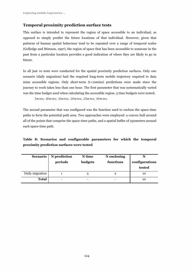
Exploring mobile trajectories …
124
Temporal proximity prediction surface tests
This surface is intended to represent the region of space accessible to an individual, as
opposed to simply predict the future locations of that individual. However, given that
patterns of human spatial behaviour tend to be repeated over a range of temporal scales
(Golledge and Stimson, 1997), the region of space that has been accessible to someone in the
past from a particular location provides a good indication of where they are likely to go in
future.
In all just 10 tests were conducted for the spatial proximity prediction surfaces. Only one
scenario (daily migration) had the required long-term mobile trajectory required to data
mine accessible regions. Only short-term (t+10mins) predictions were made since the
journey to work takes less than one hour. The first parameter that was systematically varied
was the time budget used when calculating the accessible region. 5 time budgets were tested;
5mins; 10mins; 15mins; 20mins; 25mins; 30mins.
The second parameter that was configured was the function used to enclose the space-time
paths to form the potential path area. Two approaches were employed: a convex hull around
all of the points that comprise the space-time paths, and a spatial buffer of 250metres around
each space-time path.
Table 8: Scenarios and configurable parameters for which the temporal
proximity prediction surfaces were tested
Scenario N prediction
periods
N time
budgets
N enclosing
functions
N
configurations
tested
Daily migration 1 5 2 10
Total - - - 10

Exploring mobile trajectories …
125
4.2 Approach characteristics
4.2.1 Speed-heading prediction surfaces
As described in the Speed-heading predictions section in the methodology, these are
generated by selecting a section of mobile trajectory that immediately precedes the time for
which a prediction is made (the recent behaviour period), and using the distribution of speed
and heading within that trajectory to make predictions about the possible future locations of
the moving point object. The controlling factors for this approach are therefore, the period of
time used to define ‘recent’ and whether a temporal weighting has be applied to increase the
influence of more recent points: these parameters are both concerned with the degree to
which one must look to the past when predicting the future. In order to analyse the
characteristics of this type of prediction, and to assess the influence of different
configurations of recent behaviour periods and temporal decay functions, each of the
evaluation criteria will be considered in turn. The characteristics of this approach will be
assessed by considering performance in the walking and driving scenarios.
Median verification value
An immediately obvious trend, evident for both scenarios and long-term and short-term
predictions, is that for very short recent behaviour periods, the median verification value is
very low, typically less than one (see Figure 38a to Figure 38d). By using short periods to
define the recent period, the recent behaviour lacks variation, leading to small, very focussed
surfaces, that are unlikely to coincide with the verification point (see Figure 40). As the
recent behaviour period increases, the median verification value increases, since there is
increased heterogeneity in the recent behaviour, leading to larger, less focussed surfaces.
This increases to a maximum that occurs for a recent behaviour period of about three hours
for both scenarios, and both long-term and short-term predictions. In the case of the walking
scenario, the verification value levels at off at this point and for further increases in the
recent behaviour period there is little change in the verification value. This gives the
impression that in this particular scenario, after three hours, all examples of spatial
behaviour in the parent set have been displayed, hence subsequent increases beyond this
point will have minimal further impact. In the case of the driving scenario, the median
verification value also reaches a maximum for a recent behaviour period of roughly three
hours, but then subsequently declines slightly for further increases in the recent behaviour
period. This is likely to reflect that by extending the recent behaviour period to over three
hours, a different type of behaviour is seen in the parent set, which acts as a poor predictor
for the driving behaviour.

Exploring mobile trajectories …
126
Key to temporal decay functions
Figure 38: Median verification value against recent behaviour period for
a series of speed-heading prediction surfaces
All figures a to d show the median verifiction value for a series of speed-heading prediction surfaces on the y axis, against the period of time used to define the recent behaviour (in minutes) on the x axis. Two scenarios are represented - walking and driving - and both short-term (t + 10 min) and long-term (t + 60 min) predictions have been generated for each scenario. Various approaches to temporal weighting have been tested including no weighting, temporal weighting with linear decay, and temporal weighting with various examples of decay using power functions (1.5, 2 and 3). 018
0
3 6
0
5 4
0
7 2
0
no weight
linear
power (1.5)
power (2)
power (3)
mean
Walking behaviour
a) Short-term (t + 10min) b) Long-term (t + 60min)
Median VV vs recent behaviour period
0.00
4.00
8.00
12.00
0 120 240 360
Median VV vs recent behaviour period
0.00
2.00
4.00
6.00
8.00
10.00
12.00
0 120 240 360
Driving behaviour
c) Short-term (t + 10min) d) Long-term (t + 60min)
Median VV vs recent behaviour period
0.00
0.50
1.00
1.50
2.00
0 180 360 540 720
Median VV vs recent behaviour period
0.00
0.50
1.00
1.50
2.00
2.50
0 360 720 1080 1440
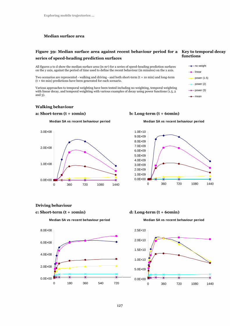
Exploring mobile trajectories …
127
Median surface area
Key to temporal decay functions
Figure 39: Median surface area against recent behaviour period for a
series of speed-heading prediction surfaces
All figures a to d show the median surface area (in m2) for a series of speed-heading prediction surfaces on the y axis, against the period of time used to define the recent behaviour (in minutes) on the x axis. Two scenarios are represented - walking and driving - and both short-term (t + 10 min) and long-term (t + 60 min) predictions have been generated for each scenario. Various approaches to temporal weighting have been tested including no weighting, temporal weighting with linear decay, and temporal weighting with various examples of decay using power functions (1.5, 2 and 3). 018
0
3 6
0
5 4
0
7 2
0
no weight
linear
power (1.5)
power (2)
power (3)
mean
Walking behaviour
a: Short-term (t + 10min) b: Long-term (t + 60min)
Median SA vs recent behaviour period
0.0E+00
1.0E+08
2.0E+08
3.0E+08
0 360 720 1080 1440
Median SA vs recent behaviour period
0.0E+001.0E+092.0E+093.0E+094.0E+095.0E+096.0E+097.0E+098.0E+099.0E+091.0E+10
0 360 720 1080 1440
Driving behaviour
c: Short-term (t + 10min) d: Long-term (t + 60min)
Median SA vs recent behaviour period
0.0E+00
2.0E+08
4.0E+08
6.0E+08
8.0E+08
0 180 360 540 720
Median SA vs recent behaviour period
0.0E+00
5.0E+09
1.0E+10
1.5E+10
2.0E+10
2.5E+10
0 360 720 1080 1440

Exploring mobile trajectories …
128
The trend with median surface area was closely related to that seen for median verification
value. Surface area tends to start low in all cases, associated with the limited heterogeneity in
the recent behaviour, then increase to a maximum between three and twelve hours, when
most examples of spatial behaviour have been exhibited. The median surface area then levels
off (in the case of driving behaviour) or decreases (in the case of walking behaviour) for
subsequent increases in the recent behaviour period. For walking behaviour in particular,
there is a clear and smooth trend of increase to a maximum, associated with a recent
behaviour period between 6 and 12 hours, before beginning to decrease again for further
increases in the period used to define recent behaviour. In this particular example, the
dramatic increase is associated with inclusion of driving behaviour, both on the morning of
the example and the previous day. This rises to a peak once this behaviour has been included,
and then begins to tail off once the recent behaviour period is increased further to include
examples of walking behaviour from the previous day. This has the effect to decrease the
range of the prediction overall, since the recent behaviour is now representing relatively
more walking behaviour, associated with slower speeds, and hence a smaller area that is
likely to be accessible.
It can be seen that the approaches that use no temporal weighting, or a temporal decay
function that results in a slow decrease in the influence of behaviour with time (such as a
linear decay function), are more affected by the trend for surface area to decrease for further
increases in the recent behaviour period. This is as you would expect since for these
approaches, points from the distant past still have considerable influence upon the overall set
(see Figure 39b). For approaches that use faster decay functions – such as negative power
decay functions - surface area tends to level off at the maximum, but not decrease for further
increases in the recent behaviour period. This is since the influence of these points from the
distant past is negligible compared to the influence of more recent points. Generally surface
area is also much greater for approaches that adopt no temporal weighting, or a linear decay
function, than for those points that adopt a faster temporal decay function. This reflects the
rapid temporal decay function providing a similar effect to decreasing the period of time used
to define recent behaviour: by giving very low weights to points from the past, the
heterogeneity of the recent behaviour is decreased resulting in much more focused, smaller
predictions surfaces, based upon the most immediate behaviour. The surface area for driving
behaviour is consistently larger than for walking behaviour, reflecting the increased range of
mechanised transport. The long-term predictions also have larger surface area, since with
more time, there are a greater region of space where you could possibly be.

Exploring mobile trajectories …
129
Figure 40: Speed-heading prediction surfaces: influence of the recent behaviour
period
In the figures below, short-term (t+10min) speed-heading prediction surfaces have been generated for the walking scenario. The prediction origin is shown as a green crosshair, and the actual destination 10 minutes later is shown as a red cross-hair. The points that are included in the recent behaviour period are shown in light green.
a: 5mins recent behaviour period
Using only 5 minutes to define the recent behaviour period, the prediction surface is very focussed in extent and direction. The surface area is very small, hence the surface is unlikely to coincide with the actual destination at the predicted time. For this reason the median verification value (and success rate) will be very low using this approach, resulting in low median prediction surface effectiveness values, despite the small surface area.
b: 24hrs recent behaviour period
Using the last 24 hours to define the recent behaviour period, a scattergun prediction surface results that is sprawling in extent and displays very little directionality. The surface area is very large, and the median verification value (and success rate) for this approach will be high, since the surface coincides consistently with the destination point. The excessively large surface areas result in low median prediction surface effectiveness, despite the high median verification values.
Images produced using the spatial history explorer

Exploring mobile trajectories …
130
Median prediction surface effectiveness
Key to temporal decay functions
Figure 41: Median prediction surface effectiveness against recent
behaviour period for a series of speed-heading prediction surfaces
All figures a to d show the median prediction surface effectiveness for a series of speed-heading prediction surfaces on the y axis, against the period of time used to define the recent behaviour (in minutes) on the x axis. Two scenarios are represented - walking and driving - and both short-term (t + 10 min) and long-term (t + 60 min) predictions have been generated for each scenario. Various approaches to temporal weighting have been tested including no weighting, temporal weighting with linear decay, and temporal weighting with various examples of decay using power functions (1.5, 2 and 3).
018
0
3 6
0
5 4
0
7 2
0
no weight
linear
power (1.5)
power (2)
power (3)
mean
Walking behaviour
a: Short-term (t + 10min) b: Long-term (t + 60min)
Median PSE vs recent behaviour period
0.0E+00
4.0E-07
8.0E-07
1.2E-06
1.6E-06
0 120 240 360
Median PSE vs recent behaviour period
0.0E+00
5.0E-09
1.0E-08
1.5E-08
2.0E-08
0 120 240 360
Driving behaviour
c: Short-term (t + 10min) d: Long-term (t + 60min)
Median PSE recent behaviour period
0.0E+00
1.0E-09
2.0E-09
3.0E-09
4.0E-09
0 180 360 540 720
Median PSE vs recent behaviour period
0.0E+00
2.0E-11
4.0E-11
6.0E-11
8.0E-11
1.0E-10
0 360 720 1080 1440

Exploring mobile trajectories …
131
Prediction surface effectiveness tends to increase with an increasing recent behaviour period
up to some maximum value, then decrease for further increases in the recent behaviour
period. The small, highly focused prediction surfaces associated with very small periods of
recent behaviour tend to only rarely coincide with verification point, leading to very low
median verification values, and hence low median prediction surface effectiveness, despite
the small surface size. The prediction surface effectiveness increases to a peak where the
median verification value is generally higher, but the prediction surface size is still quite
small. For subsequent increases in the recent behaviour period, the prediction surface
effectiveness begins to decrease, since the median verification value levels off, but the surface
area continues to rise, leading to “scattergun” predictions that are less spatially constrained.
For short-term predictions for both walking and driving scenarios, this maximum value
tends to occur after 30-60 minutes. In both scenarios (and notably for the driving example)
the peak in median prediction surface effectiveness occurs for a longer recent behaviour
period than for the long-term then for short-term predictions, suggesting that it may be
appropriate to look to the more distant past when making predictions into the more distant
future.
Approaches that adopted either a slow temporal weighting decay function (eg negative
linear), or no temporal decay at all tend to have a very pronounced peak and subsequent
drop off, hence when employing these approaches, selecting an appropriate recent behaviour
period is very important. Approaches which use a faster temporal decay function (eg negative
power functions), tend to peak later and experience a less dramatic drop off. The late peak
effect is particular evident for the negative power decay when the exponent ‘2’ is used. In this
particular scenario, long recent behaviour periods and the negative square temporal decay
functions appear to act as a very good predictor of future behaviour (see Figure 41). This
approach includes a wide variety of speed values in the recent behaviour and hence to
produce a prediction surface with more variation in the potential distance than could be
covered, leading to more of a “torch-beam” effect emanating from the prediction origin (see
Figure 42a). Another approach that performed well for the short-term walking scenario was
using a 30 minute recent behaviour period with a linear temporal decay function. This
approach tended to result in less variation in the distance that could be covered for each
prediction, leading “crescent moon” predictions, reflecting heterogeneity in the heading in
the recent behaviour, but homogeneity of speed (see Figure 42b).

Exploring mobile trajectories …
132
Figure 42: Speed-heading prediction surfaces, predicting the location of the
moving object displaying walking behaviour, 10 minutes into the future
a: Negative power temporal decay function (exponent = 2), using a recent behaviour period of 6 hours
b: Linear temporal decay function, using a recent behaviour period of 30 minutes
Images produced using the spatial history explorer
Success rate
The overall trend in success rate is to have a lowest success rate for shortest periods of recent
behaviour, with success rate increasing with the recent behaviour period up to some
maximum. For short-term predictions, this levelling off occurs for recent periods of between
30 minutes (for driving) and 60 minutes (for walking). For long-term predictions, the
levelling off in success rate tends to occur for recent behaviour periods of about 60 minutes.
As seen from the median surface area, predictions made using a very short recent behaviour
period have very little heterogeneity in the recent behaviour and tend to be very small and
focused, hence are less likely to coincide with the verification point. By using a longer
duration, there is more heterogeneity in recent behaviour, and the resulting predictions tend
be larger. This trend also impacts upon the success rate: larger surfaces are more likely to
coincide with the verification point. Even though surface area tails off beyond a point for
further increases in the recent behaviour period, the success rate of the prediction remains
level, still capturing the verification point with the same frequency.
Since fast temporal decay functions effectively decrease the heterogeneity of the recent
behaviour, resulting in smaller surfaces, they tend to have lower success rates than slow
temporal decay functions (eg linear), or speed-heading predictions that employ no temporal
weighting at all. It can be seen that this evaluation criterion rewards larger, scattergun
predictions, which are more consistent because their larger size makes them more likely to
coincide with the verification point.

Exploring mobile trajectories …
133
Figure 43: Success rate against recent behaviour period for a series of
speed-heading prediction surfaces
All figures a to d show the success rate for a series of speed-heading prediction surfaces on the y axis, against the period of time used to define the recent behaviour (in minutes) on the x axis. Two scenarios are represented - walking and driving - and both short-term (t + 10 min) and long-term (t + 60 min) predictions have been generated for each scenario. Various approaches to temporal weighting have been tested including no weighting, temporal weighting with linear decay, and temporal weighting with various examples of decay using power functions (1.5, 2 and 3).
Key to temporal decay functions
018
0
3 6
0
5 4
0
7 2
0
no weight
linear
power (1.5)
power (2)
power (3)
mean
Walking behaviour
a: Short-term (t + 10min) b: Long-term (t + 60min)
SR vs recent behaviour period
0.00
0.20
0.40
0.60
0.80
1.00
0 120 240 360
SR vs recent behaviour period
0.00
0.20
0.40
0.60
0.80
1.00
0 120 240 360
Driving behaviour
c: Short-term (t + 10min) d: Long-term (t + 60min)
SR vs recent behaviour period
0.00
0.20
0.40
0.60
0.80
1.00
0 120 240 360 480 600 720
SR vs recent behaviour period
0.00
0.20
0.40
0.60
0.80
1.00
0 60 120 180 240 300 360

Exploring mobile trajectories …
134
4.2.2 Spatial proximity prediction surfaces
These tests systematically vary the buffer distance and distance decay functions, to assess the
characteristics of these prediction surfaces. The characteristics of these spatial proximity
prediction surfaces will be assessed by comparing different configurations for two scenarios
(walking and driving), and for short-term (t + 10min) and long-term (t + 60min) predictions.
The evaluation criteria discussed in section 3.5 will be used to allow the comparison of these
different approaches.
Figure 44: The effects of the buffer distance on spatial proximity surfaces
Six long-term (t + 60min) predictions are shown for the walking scenario. The predictions have been made for three different spatial origins, using two different buffer sizes (2000 metres and 3000 metres). It can be seen that whilst the 2000 metre buffer consistently fails to coincide with the destination point, using the 3000 metre buffer, the surface captures the destination point consistently. This explains the dramatic increase in the median verification value and median prediction surface effectiveness at a threshold buffer size: spatial proximity surfaces that consistently just coincide with the verification point perform well because they are not unnecessarily spatially extensive, but those with a slightly smaller buffer distance can fail to coincide with the destination point at all.
Prediction origin a Prediction origin b Prediction origin c
20
00
m b
uff
er
30
00
m b
uff
er
Images produced using the spatial history explorer
Median verification value
The general trend for the median verification value is to have very low values for very small
buffer distances and to stay low until some threshold buffer distance is crossed. At this point
median verification value increases exponentially for increases in buffer distance. Finally,
with further increases in the buffer distance, the rate of increase of median verification value
either levels off, or decreases. This threshold buffer distance is the distance at which the
spatial proximity surface first begins to coincide with destination point for the given spatial
behaviour: for smaller buffer sizes the surface is too small to consistently “capture” the
verification point. For this threshold buffer size, the median verification point increases
dramatically from values close to zero, the very high values very quickly (Figure 44). For
unweighted spatial proximity surfaces, the median verification value then tails off for

Exploring mobile trajectories …
135
subsequent increases in the buffer distance, since there is no variation in the values within
the buffer. The linear-offset spatial proximity behaviour demonstrates very similar behaviour
to the unweighted spatial proximity surface in all situations.
For spatial proximity prediction surfaces which apply a distance decay function, the median
verification value continues to increase for further increases in the buffer size. This can be
explained by the considering the characteristics of these surfaces: spatial proximity surfaces
that apply rapidly decaying functions are characterised by high peaks at the centre
surrounded by low values as you move to the edge of the surface. As the buffer increases in
size the higher values close to the centre of the surface cover a bigger area, the destination
point is more likely to increase with these points near the centre. For the linear-offset
prediction surface, the maximum values are found in a circle around the centre. For this
decay function, the median verification value increases with increases in buffer size until the
destination is most likely to coincide with high regions on the surface, before decreasing for
subsequent increases in the buffer size, as the destination point is more likely to coincide
with the lower values close to the centre of the prediction surface.

Exploring mobile trajectories …
136
Key to distance decay functions
Figure 45: Median verification value against buffer distance for a series
of spatial proximity prediction surfaces
All figures a to d show the median verification value for a series of spatial proximity prediction surfaces on the y axis, against buffer distance (in metres) on the x axis. Two scenarios are represented - walking and driving - and both short-term (t + 10 min) and long-term (t + 60 min) predictions have been generated for each scenario. Various approaches to distance weighting have been tested including no weighting, distance weighting with linear decay, and distance weighting with various examples of decay using power functions (1.5, 2 and 3).
no w eight
linear
pow er (1.5)
pow er (2)
pow er (3)
linear offset
mean
Walking behaviour
a: Short-term (t + 10min) b: Long-term (t + 60min)
Median VV vs buffer dist
0.00
1.00
2.00
3.00
4.00
0 500 1000 1500 2000
Median VV vs buffer dist
0.00
1.00
2.00
3.00
0 2000 4000 6000 8000 10000
Driving behaviour
c: Short-term (t + 10min) d: Long-term (t + 60min)
Median VV vs buffer distance
0.00
1.00
2.00
3.00
0 10000 20000 30000 40000 50000
Median VV vs buffer distance
0.00
1.00
2.00
3.00
4.00
0 50000 100000 150000 200000 250000
Median surface area
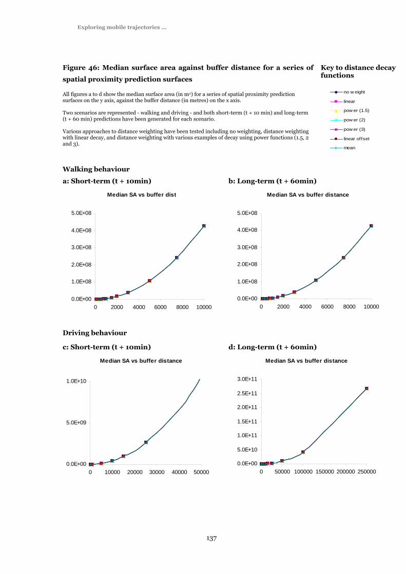
Exploring mobile trajectories …
137
Key to distance decay functions
Figure 46: Median surface area against buffer distance for a series of
spatial proximity prediction surfaces
All figures a to d show the median surface area (in m2) for a series of spatial proximity prediction surfaces on the y axis, against the buffer distance (in metres) on the x axis. Two scenarios are represented - walking and driving - and both short-term (t + 10 min) and long-term (t + 60 min) predictions have been generated for each scenario. Various approaches to distance weighting have been tested including no weighting, distance weighting with linear decay, and distance weighting with various examples of decay using power functions (1.5, 2 and 3).
no w eight
linear
pow er (1.5)
pow er (2)
pow er (3)
linear offset
mean
Walking behaviour
a: Short-term (t + 10min) b: Long-term (t + 60min)
Median SA vs buffer dist
0.0E+00
1.0E+08
2.0E+08
3.0E+08
4.0E+08
5.0E+08
0 2000 4000 6000 8000 10000
Median SA vs buffer distance
0.0E+00
1.0E+08
2.0E+08
3.0E+08
4.0E+08
5.0E+08
0 2000 4000 6000 8000 10000
Driving behaviour
c: Short-term (t + 10min) d: Long-term (t + 60min)
Median SA vs buffer distance
0.0E+00
5.0E+09
1.0E+10
0 10000 20000 30000 40000 50000
Median SA vs buffer distance
0.0E+00
5.0E+10
1.0E+11
1.5E+11
2.0E+11
2.5E+11
3.0E+11
0 50000 100000 150000 200000 250000

Exploring mobile trajectories …
138
The surface area increases exponentially with increases in buffer distance, as dictated by the
equation for the surface area of a circle. The spatial proximity surface places an enclosing
rectangle around the buffer region, however the relationship between buffer size and surface
area follows the same trend. The distance decay function has no impact on median surface
area.
Median prediction surface effectiveness
Median prediction surface effectiveness is low for small buffer sizes, since these small
surfaces do not consistently coincide with the verification point. In most cases there is a
rapid increase in median prediction surface effectiveness for the threshold buffer distance, as
the surface begins to coincide consistently with destination, but surface area is still small.
This threshold value varies depending upon scenario and the length of the prediction period.
Table 9 shows the threshold buffer distances for alternative scenarios and prediction periods.
It can be seen that larger threshold buffer distances are associated with faster moving
transportation, and for longer prediction periods, since both these increase the potential
spatial extent of movement.
Table 9: Threshold buffer distances for alternative scenarios and prediction
periods
Prediction period
t+10 mins t+60 mins
Walking ≈ 0.25 km ≈ 2 km
Sce
na
rio
Driving ≈ 15 km ≈ 100 km
Where extreme decay functions have been applied, a secondary peak can be seen for very
large buffer sizes. The secondary peak reflects the coincidence of the destination with these
very high values close to the centre. Since the surface area increases by an exponent of 2, but
the decay functions can apply an exponent of greater than 2, this can result in a high
prediction surface effectiveness values. This is a limitation of the evaluation criterion that
should be considered when assessing performance and scepticism should be expressed at the
seemingly strong performance of surfaces employing extreme decay functions. Intuitively
these surfaces with very large surface areas are poor predictors of future behaviour, however
applying extreme decay functions can lead to high prediction surface effectiveness values
(see results in appendix 3).

Exploring mobile trajectories …
139
Key to distance decay functions
Figure 47: Median prediction surface effectiveness against buffer
distance for a series of spatial proximity prediction surfaces
All figures a to d show the prediction surface effectiveness for a series of spatial proximity prediction surfaces on the y axis, against buffer distance (in metres) on the x axis. Two scenarios are represented - walking and driving - and both short-term (t + 10 min) and long-term (t + 60 min) predictions have been generated for each scenario. Various approaches to distance weighting have been tested including no weighting, distance weighting with linear decay, and distance weighting with various examples of decay using power functions (1.5, 2 and 3).
no w eight
linear
pow er (1.5)
pow er (2)
pow er (3)
linear offset
mean
Walking behaviour
a: Short-term (t + 10min) b: Long-term (t + 60min)
Median PSE vs buffer distance
0.0E+00
4.0E-07
8.0E-07
1.2E-06
0 2000 4000 6000 8000 10000
Median PSE vs buffer dist
0.0E+00
1.0E-08
2.0E-08
3.0E-08
4.0E-08
0 2000 4000 6000 8000 10000
Driving behaviour
c: Short-term (t + 10min) d: Long-term (t + 60min)
Median PSE vs buffer distance
0.0E+00
5.0E-10
1.0E-09
1.5E-09
0 10000 20000 30000 40000 50000
Median PSE vs buffer distance
0.0E+00
1.0E-11
2.0E-11
3.0E-11
4.0E-11
0 50000 100000 150000 200000 250000

Exploring mobile trajectories …
140
Success rate
Figure 48: Success rate against buffer distance for a series of spatial
proximity prediction surfaces
All figures a to d show the success rate for a series of spatial proximity prediction surfaces on the y axis, against buffer distance (in metres) on the x axis. Two scenarios are represented - walking and driving - and both short-term (t + 10 min) and long-term (t + 60 min) predictions have been generated for each scenario. Various approaches to distance weighting have been tested including no weighting, distance weighting with linear decay, and distance weighting with various examples of decay using power functions (1.5, 2 and 3).
Key to distance decay functions
no w eight
linear
pow er (1.5)
pow er (2)
pow er (3)
linear offset
mean
Walking behaviour
a: Short-term (t + 10min) b: Long-term (t + 60min)
SR vs buffer distance
0.00
0.20
0.40
0.60
0.80
1.00
0 500 1000 1500
SR vs buffer distance
0.00
0.20
0.40
0.60
0.80
1.00
0 1000 2000 3000 4000 5000
Driving behaviour
c: Short-term (t + 10min) d: Long-term (t + 60min)
SR vs buffer distance
0.00
0.20
0.40
0.60
0.80
1.00
0 10000 20000 30000 40000 50000
Median SR vs buffer distance
0.00
0.20
0.40
0.60
0.80
1.00
0 50000 100000 150000 200000 250000
Exploring mobile trajectories …
141
Success rate is only dependent upon buffer size, and not the decay function, since success
rate records simply whether the prediction surface coincides with the destination point, and
is not influenced by the internal variation within the surface. Success rate starts low for small
buffer distances, and increases rapidly as the threshold buffer distance is reached, where the
surface reaches a size where it is likely to overlap with the destination point given the
behaviour and prediction period. For further increases in the buffer size, the success rate
increases rapidly to a maximum of 1, indicating that for these buffer sizes, the surface always
coincides with the destination point.
4.2.3 Temporal proximity prediction surfaces
The temporal proximity prediction surfaces were tested in just one scenario, daily migration,
for a commute to and from work via bicycle. The temporal proximity prediction surfaces
could not be tested in the walking and driving scenarios since they need a mobile trajectory
collected over a long period of time (weeks or more), which can mined to discover which
regions of space are accessible from different locations, based upon repeated behaviour
displayed over the coarse of multiple temporal cycles. These tests systematically varied the
time budget used to calculate the potential path area from a minimum of five minutes to a
maximum of 30 minutes. Two approaches to enclosing the selected space-time paths were
tested: a convex hull and a 250metre buffer around the paths.
Median verification value
The median verification value sees an increase from zero to one between 10 and 20 minutes.
This reflects the poor performance of surfaces with short time budgets, since they have very
constrained spatial extent and are less likely to coincide with the verification value. The jump
from zero to one is a reflection of the median value being used for a Boolean surface (see
section 3.5.3).

Exploring mobile trajectories …
142
Figure 49: Temporal proximity predictions for the daily migration
scenario
Key to space-time path bounding function
buffer (250m)
convex hull
mean
a: Median verification value b: Median surface area
Mean VV vs time budget
0.00
0.20
0.40
0.60
0.80
1.00
0 10 20 30
Mean SA vs time budget
0.0E+00
1.0E+06
2.0E+06
3.0E+06
4.0E+06
5.0E+06
0 10 20 30
c: Median prediction surface effectiveness d: Success rate
Mean PSE vs time budget
0.0E+00
5.0E-07
1.0E-06
1.5E-06
0 10 20 30
Success rate vs time budget
0.00
0.20
0.40
0.60
0.80
1.00
0 10 20 30

Exploring mobile trajectories …
143
Median surface area
The overall trend is for the surface area to increase at a linear rate for increases in the time
budget: given a greater time budget, a greater region of space is accessible to you. It can be
seen that by using the convex hull to enclose the space-time paths, the surface area is up to
four times greater than when the spatial buffer around paths is used. This is since the convex
hull encloses larger regions of space between paths that was actually never visited during the
previous exhibited spatial behaviour. The spatial buffer approach is far more focused, leading
to accessibility corridors that are a better representation of the locations that were accessible
(see Figure 50).
Figure 50: Temporal proximity prediction surface: convex hull vs buffer
Two short-term temporal proximity predictions are shown for the daily migration scenario. For each prediction, the selected space-time paths can be seen (yellow lines bounded by green and red points), as can the actual destination at the predicted time (a red cross hair in the bottom right of both figures). In a, all selected space-time paths are enclosed using a convex hull (bounded by a red edge). In b, the space time paths are enclosed using a 250 metre buffer. It can be seen that the buffer has a smaller surface area, and encloses less unvisited space, notably several bridges across the Thames that are included in the potential path area defined by the convex hull. A further interesting feature is that by buffering beyond the points, the temporal proximity surface defined by the buffer coincides with the destination point (red crosshair), however the convex hull, which provides a tight fit around the points, fails to coincide with the destination point.
a: Convex hull b: 250m buffer
Images produced using the spatial history explorer

Exploring mobile trajectories …
144
The buffer approach also extends the potential path area beyond the space-time paths,
however this only occurs around the points that comprise the space-time paths themselves,
and not the space between space-time paths (see Figure 50). Using both methods, the
potential path area extends beyond the area that was accessible based upon previous
experience, however there is more control over this extrapolation using the buffer than the
convex hull, since the buffer size can be manipulated.
Median prediction surface effectiveness
For both the buffer and convex hull approaches, the median prediction surface effectiveness
is zero for time budgets of less than 10 minutes, reflecting median verification values of zero
for these time budgets. Beyond this point, median PSE tends to increase rapidly for increases
in the time budget, up to some maximum, then decreases for further increases in the time
budget (see Figure 49c). The initial increase is associated with the increase in the mean
verification value as discussed above and seen in Figure 49a. At a threshold value (about 20
minutes), the median verification value levels off, however the surface area continues to rise.
The peak is found just before this point, and for subsequent increases in surface area,
associated with increases in the time budget, the median prediction surface effectiveness
begins to decrease.
In this example, a time budget slightly in excess of the prediction period results in the most
effective temporal proximity prediction surfaces: time budget of 15 and 20 minutes work well
for a prediction of t+10mins. It can be seen that the buffer approach to enclosing the space-
time paths is far more effective than the convex hull approach, due in the main to the smaller
surface area of the resulting surfaces.

Exploring mobile trajectories …
145
Figure 51: Temporal proximity prediction surface: influence of the time budget on
the surface area
Four short-term temporal proximity prediction surfaces are shown below for the daily migration scenario. A 250metre buffer has been used to define the potential path area shown in orange. It can be seen that the surface area increases with the available time budget. The surface does not coincide with the destination for the 5 minute time budget, but does for time budgets 10, 20 and 30 minutes.
a: 5 minute time budget b: 10 minute time budget
c: 20 minute time budget d: 30 minute time budget
Images produced using the spatial history explorer
Success rate
The overall trend here is for the success rate to increase rapidly for increases in the time
budget, then to level off for further increases (see Figure 49d). Using a time budget of less
than the prediction period (eg a time budget of 5 minutes to predict location in 10 minutes),
leads to very low success rates since the surface is unlikely to coincide with the individual’s
actual destination unless they display unusually fast behaviour on that particular day. A
threshold is reached for a time budget of around 20 minutes and success rate begins to level

Exploring mobile trajectories …
146
off, suggesting that a temporal proximity prediction surface using a time budget of 30
minutes is not more likely to coincide with the verification point. This is most evident for the
tests conducted using a 250 metre buffer to enclose the space-time paths, however a similar
result can be seen when a convex hull is used. The increase of surface area for increases in
the time budget is shown in Figure 49b. Using a 250 metre buffer to enclose the space-time
paths results in consistently higher success rates than using a convex hull to enclose the
points. This is since whilst the convex hull fits tightly around all the points that comprise the
space-time paths, the buffer extends a further 250metres at the end of the paths (Figure 50).
4.3 Suitability of approaches for scenarios
Having considered the characteristics of each of the three approaches to prediction, we will
now compare how the different approaches performed in different situations. In all, five
situations are considered: short-term and long-term predictions for the walking scenario,
short-term and long-term predictions for the driving scenario, and short-term predictions for
the daily migration scenario.
Overall, speed-heading predictions outperformed the spatial proximity approach in four of
the five situations in which it was tested (see Table 10). The temporal proximity approach
outperformed both the speed-heading approach and spatial proximity approach in the one
situation in which it was tested.

Exploring mobile trajectories …
147
Table 10: Most effective configuration for each prediction approach, in each
situation.
The most effective approach in each situation is shown in bold
Prediction approach
Speed-heading
(recent behaviour
period, decay
function)
Spatial proximity
(buffer size, decay
function)
Temporal
proximity
(time budget,
bounding function)
Walking:
short-term
6 hours, power (2)
decay 500 metres, no decay -
Walking:
long-term
24 hours, power (2)
decay 3km, no decay -
Driving:
short-term 1hr linear decay 15km, no decay -
Driving:
long-term
3hrs, power (1.5)
decay 100km linear decay - S
itu
ati
on
Daily
migration:
short-term
3 hrs, power (2) decay 3km, no decay
15 (or 20) min time
budget, 250 metre
buffer
Table 11: Prediction surface effectiveness (of the most effective configuration)
for each prediction approach, in each situation.
The most effective approach in each situation is shown in bold
Prediction approach
Speed-
heading
Spatial
proximity
Temporal
proximity
Walking: short-term 1.5*10-06 1.3*10-06 -
Walking: long-term 1.9*10-08 3.6*10-08 -
Driving: short-term 3.4*10-09 1.4*10-09 -
Driving: long-term 9.3*10-11 3.5*10-11 -
Sit
ua
tio
n
Daily migration: short-
term 1.8*10-07 3.6*10-08 1.3*10-06

Exploring mobile trajectories …
148
4.3.1 Walking scenario: short-term prediction (t+10mins)
Only the speed-heading and spatial proximity approaches were tested for this situation.
Figure 52: Successful approaches for the walking scenario
Spatial behaviour was highly sinuous for the walking scenario. For short-term predictions, the speed-heading approach was most effective, since in the short-term, heading is a quite effective predictor of future direction of movement. For long-term predictions, the spatial proximity approach outperformed the speed-heading approach, reflecting the fact that heading is a less effective predictor variable in the long-term for sinuous behaviour.
Short-term prediction (t+10mins) Long-term prediction (t+60mins)
Sp
ee
d-h
ea
din
g a
pp
roa
ch
Sp
ati
al
pro
xim
ity
ap
pro
ach
Images produced using the spatial history explorer
The single most effective approach overall was a speed-heading prediction surface using a
recent behaviour period of 6 hours, and temporal weighting with power (2) decay function,
however less extreme decay functions saw a peak in the prediction surface effectiveness for a
recent behaviour period of about 30 minutes (see Table A1.3 in appendix 3 and Figure 41).
The most effective spatial proximity surface used a 500metre buffer, and no distance
weighting (see Table A1.7 in appendix 3). There is very little difference between the highest
recorded prediction surface effectiveness scores for the speed-heading approach (1.5*10-6)
and the spatial proximity surface (1.3*10-06), suggesting that the speed-heading approach
offers only minor advantages over an appropriate spatial proximity surface in this situation.
This is likely to be due to the highly sinuous nature of this scenario, which describes a figure
of eight over a period of four hours. Nevertheless, when making short-term predictions,

Exploring mobile trajectories …
149
recently exhibited speed and heading can result in a more effective prediction surface than
the most appropriately sized spatial proximity surface (see Figure 52).
4.3.2 Walking scenario: long-term prediction (t+60mins)
Only the speed-heading and spatial proximity approaches were tested for this situation.
The single most effective approach in this situation was a spatial proximity prediction
surface, employing a 3km buffer size with no weighting, suggesting that in this situation, the
speed-heading approach offers no advantage over spatial proximity surface using an
appropriate buffer size. Again the reason for this is likely to be the sinuous nature of the
walking scenario: whilst previous heading was of use as a predictor variable for short-term
(t+10min) predictions, it can tell us little about the direction of movement in the longer-term
(see Figure 52).
It is notably that the spatial proximity surfaces are more sensitive to buffer size, than the
speed-heading prediction surfaces are to recent behaviour period (Figure 52 and Figure 53).
There are very pronounced peaks around the threshold buffer size, for which the spatial
proximity surface begins to consistently coincide with the actual destination at the predicted
time; the spatial buffer sizes were selected with the scenario in mind, whereas the same
recent behaviour periods were tested for all scenarios. This suggests that speed-heading
predictions may be a more robust approach, if the choice of buffer size is not obvious for
spatial proximity prediction surfaces. Alternatively, recently displayed speed could be used to
define the buffer distance for spatial proximity surfaces for highly sinuous behaviour.
4.3.3 Driving scenario: short-term prediction (t+10mins)
Only the speed-heading and spatial proximity approaches were tested for this situation.
In this situation, a speed-heading approach employing a 60min recent behaviour period with
a temporal weighting and linear decay function records the highest prediction surface
effectiveness (PSE) score (PSE = 3.4*10-09). The most effective spatial proximity approach is
a 15km buffer with no spatial weighting (PSE = 1.4*10-09). The success of the speed-heading
approach in this situation is due to the more directed, and less sinuous behaviour displayed
in the driving scenario (see Figure 53); behaviour for which speed and heading act as good
predictor variables in the short-term.
4.3.4 Driving scenario: long-term prediction (t+60mins)
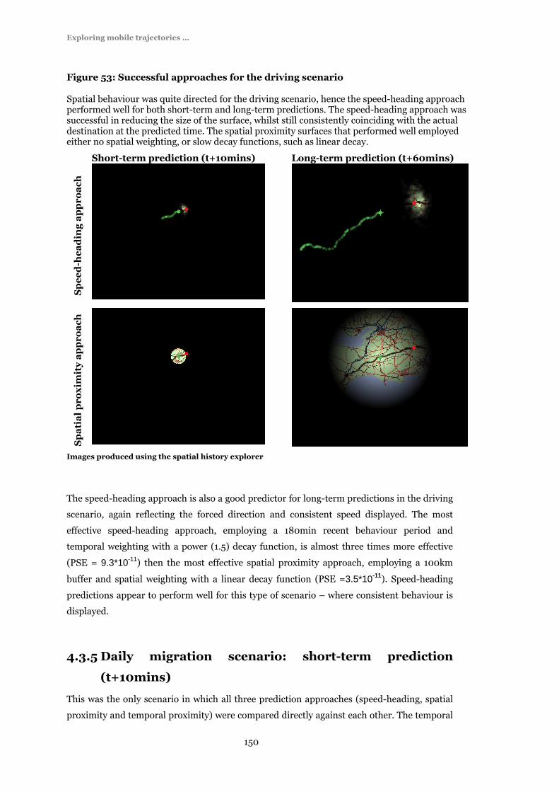
Exploring mobile trajectories …
150
Figure 53: Successful approaches for the driving scenario
Spatial behaviour was quite directed for the driving scenario, hence the speed-heading approach performed well for both short-term and long-term predictions. The speed-heading approach was successful in reducing the size of the surface, whilst still consistently coinciding with the actual destination at the predicted time. The spatial proximity surfaces that performed well employed either no spatial weighting, or slow decay functions, such as linear decay.
Short-term prediction (t+10mins) Long-term prediction (t+60mins)
Sp
ee
d-h
ea
din
g a
pp
roa
ch
Sp
ati
al
pro
xim
ity
ap
pro
ach
Images produced using the spatial history explorer
The speed-heading approach is also a good predictor for long-term predictions in the driving
scenario, again reflecting the forced direction and consistent speed displayed. The most
effective speed-heading approach, employing a 180min recent behaviour period and
temporal weighting with a power (1.5) decay function, is almost three times more effective
(PSE = 9.3*10-11) then the most effective spatial proximity approach, employing a 100km
buffer and spatial weighting with a linear decay function (PSE =3.5*10-11). Speed-heading
predictions appear to perform well for this type of scenario – where consistent behaviour is
displayed.
4.3.5 Daily migration scenario: short-term prediction
(t+10mins)
This was the only scenario in which all three prediction approaches (speed-heading, spatial
proximity and temporal proximity) were compared directly against each other. The temporal

Exploring mobile trajectories …
151
proximity approach was by the far the most effective approach in this situation, followed by
the speed-heading approach, then the spatial proximity approach. The success of the
temporal proximity approach is due to the long-term history of personal data recording the
movements of this individual. Behaviour is clearly cyclical, and many journeys, such as the
journey to work, will take similar routes at similar times. When potential path areas are
generated from this data, they act as exceptionally good predictors of future location. It
should be noted that if potential path areas were generated for aggregate data, ie the area
accessible to a large number of users over the same period, then the surface area of the
potential path area would be much greater, with the result that this approach would have a
smaller prediction surface effectiveness score.
The speed-heading prediction approach also outperforms the spatial proximity approach by
an order of magnitude in this scenario. This is since the journeys to and from work display a
clear directional trend, which can result in more focussed predictions using the speed-
heading approach that consistently coincide with the destination at the predicted time. By
comparison, the spatial proximity surfaces are very large in spatial extent, and perform badly
in this situation. The trend for the temporal proximity approach to outperform the speed-
heading approach, and for both to be more effective than the spatial proximity approach,
implies that in this situation at least, the further into the past that you look, the more
effective the prediction will be.
It is important to keep in mind that these conclusions are based upon a relatively small set of
scenarios and data collected by a small number of individuals, all of whom live and work in,
or close to, London, UK. Whilst it is possible to generalise these findings to a certain degree,
care must be taken in extrapolating these results to the wider population. Future work could
include repeating this analysis for larger datasets, containing the multiple users, to see if the
same results can derived.

Exploring mobile trajectories …
152
Figure 54: Successful approaches for the daily migration scenario
Te
mp
ora
l p
rox
imit
y a
pp
roa
ch
Sp
ee
d-h
ea
din
g a
pp
roa
ch
Sp
ati
al-
pro
xim
ity
ap
pro
ach
For the daily migration scenario, a
temporal proximity prediction surface
using a 15 minute time budget and 250
metre buffer was by far the most effective
approach (PSE = 1.1*10-06). The next
most effective approach was the speed-
heading approach, using a 6hr recent
behaviour period with a power (1.5)
temporal decay function (PSE = 1.8*10-
07). This was an order of magnitude more
effective than the most effective spatial
proximity approach, using a 3km buffer
and no distance weighting (PSE = 3.6*10-
08).
Exploring mobile trajectories …
153
4.4 User evaluation
At the end of the WebPark project, a formal period of user evaluation was conducted using
the Swiss National Park as a testbed. All project members, including the development team
had an input into the user testing strategy, and all (including the author of this thesis)
attended the week-long user test sessions, held annually for three years in the Swiss National
Park. Over 100 individuals participated in these tests and a total of 87 feedback
questionnaires were completed (Krug and Abderhalden, 2004). Test participants were given
a brief introduction to the system at the National Park House, then left to use the device
unaccompanied in the field for the duration of the day. Upon return, they were asked to
complete a feedback questionnaire. In this less formal testing scenario, it could not be
guaranteed that all users would utilise all of the system functionality, hence the response rate
to some questions was low. Questions relevant to this thesis, discussed below, relate to the
performance of alternative geographic filters for mobile information retrieval, and a trekking
application that built on some of the time geography concepts developed in this thesis to
estimate time to completion for known walking routes. The WebPark system allows the user
to specify the subject and geographic component of their query separately. The subject can be
specified either by selecting categories from an ontology specified by the Park managers, or
by a keyword search, similar to Internet search engine. The geographic component can be
specified by selecting one of three options (see Figure 29): search whole park (no geographic
filter), search around me (spatial proximity surface filter), search ahead (speed-heading
prediction surface filter).
For the spatial proximity filter, the buffer size can be specified from a drop down menu. For
the search ahead filter, the time to predict ahead can similarly be specified from a drop down
menu (see Figure 29). This allowed users to tailor the geographic component of their filter
according to their needs. The speed-heading prediction surface employed a 10 minute recent
behaviour period and no temporal weighting, hence the prediction reflects the user’s
behaviour from the recent past. No accessibility or visibility filters were implemented as part
of the WebPark system.
The feedback from users about the geographic filters can be seen in Figure 55. The search
around me filter was considered to provide the most relevant information with two thirds of
the respondents saying that this provided “extremely relevant” results, and over 90%
claiming that results were either “extremely relevant” or “relevant”. The search ahead filter
also performs well, with a similar number (89%) claiming that results were either “extremely
relevant” or “relevant”, and half claiming that the results were “extremely relevant”. The
geographic filters clearly outperform the “search whole park” option, where 43% of
respondents claimed that the information provided using this option was either “less
relevant”, or “not relevant” (Krug and Abderhalden, 2004). Considering the geographic

Exploring mobile trajectories …
154
component of the user questions identified in the visitor shadowing study (see Appendix 1) it
is unsurprising that the spatial proximity filter was considered to provide the most relevant
results, since the majority of the questions referred to the user’s current location for
geographic context. The good performance of the “search ahead” filter suggests that this can
also perform well, and that people are receptive to the idea of alternative notions of
geographic context when making queries from mobile devices.
Figure 55: Relevance of results using different geographic filters
Responses to the question “How relevant did you find the results using the following search functions?”, from WebPark Summer testing 2004, in the Swiss National Park. The questionnaire was completed by 87 respondents.
Visitors were also asked about further geographic filters which were not implemented in the
WebPark system (see Figure 56). These were;
A “visible” filter: retrieving only results which are visible to the user;
A “concealed” filter: retrieving results which are close by, but concealed from view by
the terrain;
A “travel time” filter: ranking results by the time taken to travel to the associated
location, hence results are ranked by temporal proximity, as opposed to spatial proximity.

Exploring mobile trajectories …
155
Figure 56: Perceived benefit of alternative geographic filters
Responses to the question “How beneficial would you find the following search options?” from WebPark Summer testing 2004, in the Swiss National Park. The questionnaire was completed by 87 respondents.
0% 20% 40% 60% 80% 100%
Accessible
Concealed
VisibleNo answer
Useless
Less beneficial
Beneficial
Extremelybeneficial
Responses suggest that the visibility filter would provide the greatest benefit to mobile users,
with one quarter of respondents finding this “extremely beneficial”, and 44% considering it
“extremely beneficial” or “beneficial”. A travel time (temporal proximity) filter is also
considered to be of use, with a similar number (45%) considering this “extremely beneficial”
or “beneficial”, although fewer (16%) chose the top category. The concealed option is
considered to be of the least benefit with only 25% considering this “extremely beneficial” or
“beneficial” and one third thinking it would be “less beneficial” (Krug and Abderhalden,
2004). Interestingly one third of respondents did not answer this question, suggesting that
the use of these geographic filters may still be difficult to imagine, and hence difficult to
express an opinion about.
The final application relevant to this thesis which was evaluated as part of the WebPark
Summer testing 2004 was the trekking application. This application plots the long profile of
known walking routes, with distance along the route on the x-axis against elevation on the y-
axis (see Figure 57a). Anecdotal evidence suggested that this application was extremely
useful, providing an immediate visual representation of the progress through a route in
terms of distance on the ground, and the elevation left to climb. Using the principles of the
time geography school, the time taken to travel along the route was also calculated, making
the assumption that speed along the ground would vary according to the steepness of the
terrain. The first version of the application used speeds dictated by Naismith’s rules (Fritz
and Carver, 1999, Langmuir, 1995, Scarf, 1998). Subsequent versions used the mobile
trajectories collected by previous users to data mine speed rules. As a result estimates could
be provided about the time remaining for the traversal of a route, based upon previous

Exploring mobile trajectories …
156
experience (see Figure 57b), hence this application used the same principle as the
accessibility filter, however it was applied in only one dimension, distance along the route.
Figure 57: User interface for the trekking application
The trekking application was developed as part of the WebPark project, and provided information about progress along a known route in a National Park or outdoor recreational area. The application displays elevation against distance along the route (a), or the travel time along the route (b), based upon established speed rules, or previously displayed behaviour. For the travel time route profile, it can be seen that the uphill sections are more drawn out (reflecting slower ascent), and the downhill sections steeper (reflecting faster descent).
a: Distance along route vs elevation b: Travel time vs elevation

Exploring mobile trajectories …
157
Figure 58: Benefit of the trekking application
Responses to the question “How beneficial did you find the Trekking Application?”, from WebPark Summer testing 2004, in the Swiss National Park. The questionnaire was completed by 87 respondents.
0 20 40 60
No answer
Useless
Less beneficial
Beneficial
Extremely beneficial
percentage
Figure 59: Accuracy of the trekking application travel time predictions
Responses to the question “How did the travel time predictions made by the Trekking Application compare to your progress?”, from WebPark Summer testing 2004, in the Swiss National Park. The questionnaire was completed by 87 respondents.
0 10 20 30 40
No answer
I was slower than predicted
I was faster than predicted
Prediction about right
percentage
Respondents were first asked how beneficial they found the trekking application (Krug and
Abderhalden, 2004). 90% of respondents replied that it was either “extremely beneficial”
(52%), or “beneficial” (43%), suggesting that information related to travel times and
accessibility is of great importance to mobile users. As a follow-up question, users were asked
how their progress compared to the travel time predictions made by the trekking application.
38% of respondents did not answer this question suggesting that they either did not use this
functionality, or did not remember using it. Of the remainder, just under one third (30%)
replied that the prediction was about right, one fifth (20%) replied that they were slower than

Exploring mobile trajectories …
158
the prediction, and about one eighth (12%) said that they were faster than the prediction.
This suggests that whilst there is no systematic error with the travel time predictions in this
particular context, there is a need to personalise the travel times to reflect individual
behaviour, since there is evidently variation in the time taken to complete walking routes.
Data mining personalised speed rules is quite possible, however, it requires a large volume of
data about that individual to be generated, providing examples of walking behaviour in a
variety of different conditions.

Exploring mobile trajectories …
159
5 Discussion
Discussion Abstract
This chapter commences with a discussion of geographic context for mobile information
retrieval, and suggests that by concentrating on providing information related to the
spatial proximity of available services, location-based service providers have missed an
opportunity to consider the more general problem of providing generic information
sources that are geographically relevant (based on a range of criteria) to mobile users of
handheld devices. The contrast between the expected take-up of location-based services
and the current reality is presented as motivation to create more sophisticated mobile
information retrieval tools. The utility of four potential geographic filters, that have been
introduced at various points in this thesis are then discussed: the “search around me”
filter; the accessibility filter; the “search ahead” filter and the visibility filter.
Next, the effectiveness of different geographic filters as prediction surfaces is considered.
The assumptions underlying the evaluation criteria are restated (that effective prediction
surfaces tend to coincide with the verification point, that the surfaces are spatially
constrained, and that they are consistent over a series of predictions). The characteristics
of different prediction approaches are then contrasted.
Next, the utility of geoVisualization and interactive time geography for the exploration
and analysis of mobile trajectories is discussed, and some insights gained from visual
analysis are described.

Exploring mobile trajectories …
160
5.1 Geographic context for mobile information
retrieval
Within the field of mobile telecommunications, the focus for information retrieval on mobile
devices has thus far been the emerging field of location-based services (LBS). LBS are, by
definition, concerned with providing information about the services that are in some way
geographically relevant to your current location: an implication of this approach is that you
wish to purchase some service, be it consumables from a nearby store, or geographically
relevant information from a service provider. In a taxonomy of mobile location services,
Giaglis (2003) identified six broad categories of services: emergency, navigation,
information, advertising, tracking and billing. The commercial aspect of the majority of these
services is clear, even in the need to commodify information services, where the subclasses
“travel services”, “mobile yellow pages” and “infotainment services” were identified. There
has been far less attention to searching for freely available information sources using the
mobile Internet, or attempts to compare the similarity of the geographic footprint of free text
web documents with the geographic footprint associated with a user’s query. This is at odds
with the experience of the “static” Internet, where search engines rank web documents
according to the relevance to the user query: the emphasis here is on providing relevant
information (which may contain information about services), hence people are accustomed
to accessing information sources without the barrier of cost. In the world of mobile
information retrieval, we are in danger of only providing information about this subset of
information – services – and not tackling the larger problem of providing geographically
relevant information from freely available web documents.
There are several possible reasons why mobile information retrieval has thus far been
primarily concerned with services rather than information sources. First, it has proved easier
to identify the geographic footprint of many services than information sources generally: so
called “service-scopes”. Many databases already exist detailing available services, with spatial
information linking that service to an unambiguous location in the physical world
(upmystreet.com, 2005, Yell Group, 2005a, Google, 2005). Many such databases existed in
paper form for decades prior to the existence of the World Wide Web (Yell Group, 2005b), all
requiring a significant investment in terms of initial creation and subsequent maintenance
and curation to ensure the currency and accuracy of the information listed. Established
geocoding processes (Raper et al., 1992) have allowed toponyms and addresses to be
converted into spatial coordinates, creating point of interest databases allowing these
resources to be processed by conventional GI Systems. Usually these services are associated
with a single point location, specified by the address listed for a given service. The availability
of an unambiguous point location associated with every service has made the development of
location-based services much easier. The notion of geographic relevance is then based upon

Exploring mobile trajectories …
161
spatial proximity – which could be Euclidean or network distance - between a point location
defining the user query (for example a toponym or postcode), and the point location
representing the location of the required services (Jones et al., 2004).
Geographic information is also found in web resources: as mentioned in the literature review
(see section 2.7.2) Silva et al (2004), in a study of Portuguese resources, found references to
administrative areas alone could be found with a frequency of over 2 references per
document. The research conducted within the emerging field of Geographic Information
Retrieval suggests that the geographic footprints associated with web resources are far more
ambiguous and complex than those associated with services in point of interest databases.
Web documents may refer to several, geographically distributed, toponymns, identifying the
broad geographic scope that the document may refer to (Silva et al., 2004). Moreover,
toponyms are rarely unique: the word “Newcastle” forms part of at least 12 toponyms in the
UK alone (Ordnance Survey, 2005a). Disambiguating this plethora of spatial information to
identify the geographic focus of a document is a non-trivial procedure, for which research is
ongoing to find a robust solution (Amitay et al., 2004). The application of gazetteers and
construction of geographic ontologies has allowed progress to be made in this area, however
the complexity of the geographic footprint associated with web resources is still likely to be
far more complex than those associated with the services listed in custom FOI databases.
The main reason cited for the complexity of the geographic footprints associated with web
resources is that documents will frequently refer to more than one toponym in the text
(Amitay et al., 2004). Where these multiple toponyms display clustering in space, this may
assist in identifying the geographic focus of these resources, however when they are
geographically distant, the presence of multiple toponyms becomes problematic. A further
complicating factor, that has received less attention amongst the geographic information
retrieval community, is that whilst gazetteers and geocoding tools can assist us in identifying
the locations to which toponyms and addresses refer to in spatial coordinates, many natural
features are not stored in gazetteers and hence cannot be processed in the same way. The
process of identifying the geographic footprint of natural feature is more complex, since
many geographic phenomena, such as mountains and forests, do not have discrete
boundaries but can display the characteristics of continuous phenomena on the one hand, or
there may be no true defensible consensus as to what constitutes certain geographic concepts
on the other (Fisher and Wood, 1998, Fisher et al., 2004). All these factors have made the
identification of the geographic footprint associated with a web document very problematic.
A further reason for the focus of services in mobile information retrieval is likely to be related
to the more commercial nature of mobile telecommunications when compared to the fixed
Internet. The physical infrastructure of the Internet is not owned by any one single
organisation, but is a network of networks, run collaboratively by a large number of public
and private organisations (Berners-Lee and Fischetti, 1999). The majority of mobile

Exploring mobile trajectories …
162
telecommunications networks, however, are designed to run independently and are owned
privately by profit making organisations (3, 2005, O2, 2005, Orange, 2005, T-Mobile, 2005,
Vodafone, 2005b). These organisations have made significant investment in both the
network infrastructure, and the license to build third generation networks (VisionGain,
2003). Given this context it is perhaps unsurprising that the mobile Internet, accessed via
the networks of privately owned organisations, has concentrated on services that can be
purchased at a price, as opposed to information that can be accessed for free.
Nevertheless, this promotion of location-based services has failed to see the take-up
anticipated when they were first proclaimed as the “killer app” of the mobile Internet (Berg
Insight AB, 2005). Various reasons have been suggested as to why these services have failed
to perform as expected, including slow and imprecise positioning technology, and lack of
processing power and functionality in client handsets, however the primary reason for the
slow take up identified in a market report by Berg Insight AB (2005) was:
“… the services offered up until today have simply been too slow and
complicated to use.” (Berg Insight AB, 2005)
Unlike desktop users, who can devote their full attention to a task with limited external
distraction, mobile usage tends to take place in an environment where the cognitive load on
the user from external sources is higher: rather than a blank wall behind their screen there is
a dynamic world, within which they are moving and interacting. Research by Palm (Ostrem,
2002) has suggested distinct differences in usage behaviour between desktop and handheld
computing, with handheld usage being characterised by multiple, short sessions, as opposed,
to the few, long sessions displayed in desktop usage. This suggests that mobile users may be
more in need of filters to ensure the relevance of the information that they receive, than their
static counterparts, since they have neither the time, nor the same level of attention, to
manually refine information searches themselves, in the way that users accessing the
Internet over static desktop devices have become accustomed to. A variety of geographic
filters, deployed in different situations, may assist in increasing the relevance of retrieved
information, and may possibly lead to the anticipated take-up of mobile information retrieval
and mobile location services.
In order to retrieve geographically relevant information, relevance ranking based upon the
similarity of the geographic footprints of Internet resources (or services), and the geographic
footprint associated with a user’s query must occur. Users of static machines, with mouse
interfaces and keyboard interfaces may define the spatial extent of their query in a number of
ways, for example clicking on a map (Jones et al., 2002), or typing a toponym or postcode
(Yell Group, 2005a). Alternatively, a linear feature, such as a road or river, could be selected
from a map – or “heads-up” digitised manually - and used as the geographic footprint of a
query. Finally an areal geographic footprint may be defined, either by specifying a spatial

Exploring mobile trajectories …
163
extent on a map (Google, 2005) , or by entering a toponym associated with an areal feature
(such as “Greater London”, or “England”). Whilst these options are also available to mobile
users, as this thesis has suggested, there may be more automated and intuitive ways of
identifying the geographic extent of their query.
5.1.1 The “Search around me” filter
This is the current paradigm in LBS, where results are ranked according their distance from
the user’s current location. This is a reasonably unsophisticated filter that may not take
account of network distances, speed of travel, or the spatial behaviour of the individual
making the query. Some services allow users to vary to spatial extent of their query by
changing the buffer size (WebPark, 2005)
One usage scenario that is not currently handled is spatial proximity alerts for Internet
resources. A historian, on their day-to-day movements about their home town of London,
may wish to be alerted to resources related to the Great Plague, as they pass the locations
associated with those resources. This requires a dedicated agent working in the background,
searching for resources linked to an individual’s declared interests, filtering those results by
spatial proximity filter (Mountain et al., 2003), and providing an alert when a resource is
identified as being relevant on the subject and situational level (Saracevic, 1996a). Such a
system is likely to require a great deal of tuning, to ensure that it provides novel information,
and that the frequency of information is not too overwhelming on one hand, or too
infrequent on the other. Push services based upon agent technology such as these could offer
one novel approach to accessing resources on the mobile Internet, however the spatial
proximity filter described here is only one of the potential geographic filters that could be
applied to increase the relevance of retrieved information.
5.1.2 The accessibility filter
Whilst the current paradigm of LBS has been proximity in space, we have also considered the
case of proximity in terms of travel time. This is sensitive to that fact that accessibility is
rarely homogenous in all directions; transportation networks, and physical and
administrative barriers, result in a complex geographic footprint for the region of space that
is accessible within 20 minutes. In addition certain regions may be restricted due to
authority constraints (Hagerstrand, 1973), either at specific times or permanently, and these
regions could be masked out. This could include private property, live firing ranges in
outdoor recreational areas (Dartmoor National Park Authority, 2005), or public access land
closed temporarily under a temporary prohibition order from the land owner (1999).
An example of a query using a temporal proximity filter that is currently unsatisfied using
existing search engines might be a parent, searching for child care services within 20 minutes

Exploring mobile trajectories …
164
drive of their home. Such a query requires the geographic location associated with web
documents to be known, and an algorithm to calculate the region of space accessible to a
person, within 20 minutes from a given location. Queries such as these are likely to be of use
to users of both the static and mobile Internet.
5.1.3 The “Search ahead” filter
A problem that has been identified with the spatial proximity “search around me” filters is
that for fast moving mobile users, by the time the results have been received, they are no
longer relevant since the user has moved on. Even at slow speeds, users may wish to receive
information that will be relevant for a longer period of time than the immediate future. One
can imagine at least two scenarios: providing information relevant to where the user will be
at an instant in the future (for example a passenger in a car searching for places to stop and
eat in one hour’s time) and results relevant to an interval in time (in the same scenario,
searching for the restaurants they are likely to pass in the next hour).
One scenario of use can be drawn from the WebPark project (Krug et al., 2003). A visitor to a
National Park may be interested in finding the areas where wild orchids are likely to found
over the course of the next hour of their walk. Such a query requires some prediction
algorithm, to calculate the region of space they are likely to pass during the next hour, and an
approach to defining the geographic footprint associated with the distribution of wild
orchids. In the WebPark project a search ahead algorithm was implemented that allowed the
user to search for results that were ahead of them, and allowed them to specify the cut-off
time period for the prediction. A species application modelled the distribution of different
animal and plant species, based upon elevation and land cover, defining the geographic
footprint associated with each species depending upon their habitat preferences (WebPark,
2005). The combination of these components has allowed such queries to be satisfied for
visitors to the Swiss National Park.
5.1.4 The visibility filter
The final suggested geographic filter is based upon the region visible to an individual, and
can be calculated knowing an individual’s location (and ideally height) with a Digital
Elevation Model in a GI System. Testing in the Swiss National Park has suggested that
mobile users tend to be more engaged in the world around them than static users, and more
inspired by the things they see. In a region of extreme terrain, an individual may be
motivated to find out more about a distinctive distant peak that is omnipresent on the
skyline, and less interested in the closer landforms that are hidden by foreshortening.
In a scenario that combines a visibility filter with newswire resources, an individual may
witness an established fire in a factory from a distance, and wish to search for any up-to-date

Exploring mobile trajectories …
165
news reports that may have already covered this story. This requires a viewshed to be
calculated to refine the search to the region that the user can see, and the geographic
footprint associated with the newswire documents to be extracted, stored and indexed in a
scalable way, to allow relevance ranking to occur on the basis of the query and documents’
footprints.
5.1.5 Combining filters
Beyond the individual application of these filters, there is the possibility of combining them
together, or with external sources of information, to generate yet more sophisticated filters.
For example, an accessibility filter could be combined with a “search ahead” filter to produce
a surface that represented the locations that were both accessible, and likely to be visited.
External sources of information could include network and land-use to model constraints. A
Boolean mask of private land could be used to exclude areas that are known to be
inaccessible. Similarly, network-based routing algorithms, such as the Djikstra shortest path
algorithm, could be combined with these filters as a means of combining the deterministic
network-based routing with more personalised information related to the previous behaviour
of an individual or individuals.
5.1.6 Mobile information retrieval based upon historical
spatial data
One alternative use of positional data not discussed at length in this thesis is to analyse
historical records of spatial behaviour to evaluate how information provision itself
influenced user behaviour, and possibly use this information in ‘page ranking’ algorithms.
There is a clear parallel here with the patent filed by Google Inc - Information retrieval
based on historical data - (Acharya et al., 2003), where the length of time a user visits a
particular page, following a search on the fixed Internet, can be used to assess the relevance
of that page, with one interpretation being that information seekers will dwell for longer on
more relevant results.
In mobile information retrieval, each result has a spatial footprint associated with it.
Following a search for mobile information, the user’s location can be tracked to see which, if
any, of the suggested results were visited and how long was spent at that location, and
whether they subsequently visited further results from the list (Briggs, 2006). This
information could then be used to influence the ‘rank’ of the information sources associated
with those locations. Just as with the fixed Internet case, care must be taken when
interpreting results. In the fixed Internet, a short dwell time does not necessarily imply a less
relevant site – on the contrary it could indicate a well organised page that allows an
information seeker to resolve their anomalous state of knowledge quickly. Similarly, a very

Exploring mobile trajectories …
166
relevant feature in the physical world may not be visited for a long duration, but may provide
an individual with the service or information that they require: an opportunity to buy a
product, a place to park a car, or a successful rendezvous at an agreed location are all
examples where relevant information was provided but an individual need not dwell for long
at the location associated with that information source. Similarly, subsequently visiting other
locations on a list does not imply that the information source associated with previously
visited locations is less relevant or previous information sources failed in themselves to
resolve an anomalous state of knowledge. There is clear opportunity for further research in
this area.
5.2 Geographic filters for prediction
Given the potential for geographic filters for mobile information retrieval, the geographic
filters implemented as part of this study will now be reassessed. A stated objective of this
thesis is to implement a geographic filter that ranks information by the likelihood of an
individual going to the location associated with that information. An interesting counterpoint
to this approach is that relevant information could itself be the motivation to change your
spatial behaviour. For example, discovering that a site of great interest to you is located along
a path that doubles back on your current heading, may be the motivation to take that path.
The geographic context of an individual is complex, dynamic, and inherently uncertain. This
thesis has attempted to widen the scope of what is considered to be “spatially relevant”, and
tailor this context based upon personal spatial behaviour. Three geographic filters have been
developed as part of this thesis (spatial proximity, temporal proximity, speed-heading
prediction) and all have been tested for their ability to predict the future location of moving
point objects. In the following sections, the evaluation criteria used to describe the
characteristics and effectiveness of the prediction surfaces will be assessed. Next each filter
will be discussed in turn, to see how well it met its objectives, and how it could be used for
mobile information retrieval.
5.2.1 Prediction Evaluation criteria
The prediction surfaces evaluation criteria were based upon three key assumptions about
effective prediction surfaces:
1. Effective prediction surfaces coincide with the actual destination at the predicted
time; where a surface has internal variation, the destination point coincides with
high values;
2. Effective prediction surfaces are spatially constrained;
3. Effective prediction surfaces are consistent when making a series of predictions

Exploring mobile trajectories …
167
Based upon these assumptions, four criteria were defined that could describe the
characteristics of the approaches to prediction in different situations. The aim of these
criteria was to be able to describe the characteristics of different approaches to prediction, in
a range of situations, and to allow direct comparison of the effectiveness of these different
approaches in a clear and unbiased manner. Of the four criteria, three were predominantly
descriptive, attempting to assess how changes in input parameters influenced the character
of the resulting surface. Only one of the criteria – prediction surface effectiveness – was used
to compare the effectiveness of different approaches.
Median prediction surface effectiveness
Prediction surface effectiveness (PSE) is defined by verification value divided by surface area,
and used to compare the performance of any two prediction surfaces in the same situation.
Median PSE was used to compare the performance of a particular approach in a particular
situation, measured over a series of predictions. Using the median prediction surface
effectiveness reduced the influence of the small number of surfaces with extreme scores,
which could skew results to give high mean verification values for inconsistent approaches.
Another limitation to using the median value for Boolean surfaces, is that there is the sudden
jump in the median verification value, and hence also the PSE, as described above. When
using this measure with Boolean surfaces, it is wise to also consider the success rate, to
distinguish those approaches which are reasonably consistent (eg 51% success rate) from
those which are very consistent (eg success rate = 100%).
5.2.2 Spatial proximity
This thesis has considered only Euclidean distance, but network distance can also be used
rank information on the basis of proximity. Spatial proximity was included primarily as a
control as a prediction surface: it operates on the assumption your current future location
will be correlated to your current location, which can reduce search spaces down from the
global to the local. The most effective surfaces tended to be those with either no spatial decay
(see Table 10), or slow decay functions. This is unsurprising since all tests were conducted in
scenarios in which the point object was moving, hence a peak in values at the current
location - associated with fast decay functions - is less likely to coincide with the location of
the object in the future. Offset linear spatial proximity functions were developed specifically
to account for anticipated movement from the current location. These offset spatial
proximity surfaces tended to perform better than fast decaying functions, but not as well as
those with no decay.
Spatial proximity surfaces performed much better when highly sinuous behaviour was
displayed - relative to speed-heading predictions - than when continuous movement in a

Exploring mobile trajectories …
168
particular direction was displayed. In the absence of any other information, proximity in
space to the last known position is a reasonably effective approach to predicting future
location, however an appropriately sized cut-off distance should be selected. Such a distance
could be calculated from current speed, but in an absence of this information and choosing
arbitrary buffer distance, the prediction surface is likely to be either much too big (eg for slow
moving objects) incorporating a great deal of space that is unlikely to be visited, or much too
small (eg for fast moving objects), and unlikely to coincide with the actual destination. There
is also no way to prevent the selection of inaccessible and invisible information resources
with this filter, and thus it should best be used with filters to exclude results with subfilters.
5.2.3 Temporal Proximity
Temporal proximity prediction surfaces built directly upon the principles of time geography,
and the potential path area, dictating the region accessible given time restrictions. Increasing
the time budget increases the region of space available to an individual. The most effective
temporal proximity prediction surfaces used a time budget slightly longer than the prediction
period. A buffer around the space-time paths that comprise the potential path area was
found to be a more effective way of defining the surface than a convex hull, which was more
likely to include previously unvisited space. This approach defined accessibility corridors,
based upon previous experience, and was found to be the most effective approach to
predicting future location for the “daily migration” scenario in which it was tested.
Of the measures of temporal proximity developed and described in section 3.4.2, only the
potential path area was used to define temporal proximity; these define the region of space
accessible within a specified time budget, but provide no indication about which is the more
accessible of two locations within the surface boundary. Using isochrone surfaces and graded
accessibility surfaces provides variation within the surface, giving an indication of the degree
of separation in time. This could be a fruitful area for future research. Isochrone surfaces can
be used to create space-time prisms (Forer, 1998, Lenntorp, 1978, Miller, 1991, Mountain et
al., 2003) that are based upon previous experience, rather than simplistic assumptions about
movement.
In this thesis, when defining the region accessible to an individual in a given time budget,
this was always based upon the previous behaviour of that same individual. Forer (1998)
argued that many of the constraints (such as economic or mobility) experienced by
individuals are in fact generic and can be applied to others. By contrast the original
principles of Hagerstrand (1973) considered the movements of individuals and made
conclusions form these. Forer suggested that the anonymous approach is the correct one
since it retains individual privacy. There is the opportunity to data mine the behaviour of
many individuals, to define the region of space accessible in new locations, or using routes
that are unvisited by this individual. Recent technological developments, such as the

Exploring mobile trajectories …
169
convergence of positioning and mobile telephony technologies (Camara, 2003, Goker et al.,
2004, Pinpoint Faraday, 2005, Swedberg, 1999) allow mobile trajectories to be gathered on a
large scale, and this data could be used to define temporal proximity surfaces (Ratti et al.,
2005) based upon such aggregate behaviour.
Given larger volumes of data, there will be an increased need to classify the spatial behaviour
into different categories (Blythe et al., 1999, Laube, 2001). Temporal proximity surfaces
could be defined for different types of transport (eg walking, private car, public bus); an
individual’s current behaviour, or transport preferences, could then be matched to these
classes. As described in section 4.4, work has already been undertaken in developed
personalised speed rules based upon previous experience. This could be extended to develop
personalised accessibility networks, based upon transportation preferences, where travel
times are mined from the aggregate behaviour of large numbers of users. Transportation
networks tend to display diurnal variation in congestion and speed of movement that is to
some degree predictable. Temporal proximity surfaces could be developed, based upon
aggregate behaviour, that model accessibility at different times of day, days of the week, or
for specific events such as sunny bank holidays, or a football match (Ratti et al., 2005). The
aggregate behaviour of large numbers of individuals is also likely to be of interest to urban
planners, who could use information about the numbers of people moving at different times,
and the speed of movement, when planning transportation networks and services (Ratti et
al., 2005). Thus there is the opportunity to filter information based upon personal
experience, the aggregate experience of all other users, or the experience of others who
display similar patterns of spatial behaviour.
5.2.4 Speed-heading predictions
Speed-heading predictions were found to be most effective in situations where movement
was reasonably consistent in terms of speed and heading, such as journeys where the
intention is to travel between two locations by the shortest route, as displayed in the driving
and daily migration scenarios. They performed less well for highly sinuous behaviour, such
as the walking scenario. There is a compromise in specifying a recent behaviour period,
between including too much “irrelevant” behaviour from the distant past, and including
sufficient variation to account for the individual’s unpredictable future behaviour. It was
found that relatively long periods of recent behaviour, with relatively fast decay functions,
were most effective in predicting future location. This appears to offer a compromise
between using appropriate mean values for speed and heading, and ensuring that there is
also sufficient variation displayed.
Predictions may be improved by identifying breakpoints in the mobile trajectory associated
with changes in spatial behaviour, for example getting off a train and onto a bus, or getting
into a car following a walk. One hypothesis that could be tested in the future is that a more
Exploring mobile trajectories …
170
effective prediction may be achieved if only the behaviour after the last breakpoint is
considered. There is inherent uncertainty when making predictions, and this may be best
represented through the inclusion of a noise component to the prediction, to avoid situations
where very uniform previous behaviour leads to very precise predictions. Kalman filters
discussed in section 2.4 use a noise and prediction component, and vary the influence of
noise depending upon feedback from previous predictions (Elnagar, 2001, Vasquez and
Fraichard, 2004). Kalman filters have mostly been applied for prediction periods of a few
seconds (Vasquez and Fraichard, 2004), however some studies have attempted to use them
to predict the future location of moving objects in the longer-term future (Li, 2002). Such an
adaptive approach, that could systematically assess which configurations have been most
effective in the past, could be useful for defining which parameters to apply for subsequent
predictions.
Finally this approach has predicted likely future locations based upon speed and heading: the
distribution of turning angles is not considered in the prediction. Future work could include
modelling spatial behaviour using speed and turning angles. This could be applied to the task
of classifying spatial behaviour (Blythe et al., 1999), identifying breakpoints in the mobile
trajectory, and uncovering relationships between the spatial interactions of two or more
entities (Laube and Purves, 2005).
5.3 GeoVisualization and Interactive Time Geography
Forer (1998) identified two key research questions relevant to time geography: what
approaches, that have been previously constrained by technology, look likely to yield suitable
results, and what existing models of space-time may be suitable for implementing the
concepts developed by time geography. When time geography first emerged, researchers
were more limited in terms of the data and computing resources available. In an attempt to
reassess how these concepts could be applied to real data as part of this thesis, first mobile
trajectories were collected at a fine spatio-temporal resolution, describing the spatial
behaviour of several individuals, over a prolonged period of time, and in a variety of
representative situations. Next, the time geography concepts were implemented in an
interactive environment, the spatial history explorer, which allows space-time paths and
potential path areas to be extracted, that are based on the previous behaviour of mobile
individuals. This development was necessary due to the poor handling of the temporal
dimensions within existing GI Systems (Peuquet, 1999). Analysis of mobile trajectories
within this environment has led to considerable insight into individual patterns of
movement. These insights include:
• Individuals tend to display very repetitive motion patterns, that recur on a variety of
temporal scales;

Exploring mobile trajectories …
171
• Future behaviour is to some degree predictable, based upon short-term and long-
term previous behaviour;
• For the datasets collected, distinct classes of behaviour can be discerned, that reflect
alternative transport preferences and tasks.
These insights led directly to the development of speed-heading prediction and accessibility
filters described in this thesis.
Applying a traditional spatial approach to modelling movement, Forer (1998) has suggested
that distance and travel time are interchangeable entities with travel time often being a more
relevant parameter for modelling human behaviour. By creating potential path areas base in
an interactive environment, the notion of a temporal proximity (eg within 5 mins) could be
contrasted to spatial proximity (eg within 500 metres). This approach has allowed
comparison between the spatial behaviour of different individuals, and the complex temporal
characteristics of temporal proximity which arise as a result of predictable events. Whilst the
distance in space between two locations is a fixed variable, travel time is dynamic, changing
on a range of temporal scales from the short (e.g. daily rush hours) to longer periods of time
(e.g. evolution of the transportation infrastructure).
There is much further research that could be conducted in the area. As mentioned in section
5.2.3, aggregate analysis could yield information that would be extremely useful to those
planning public services such as transportation networks, and used as the geographic context
for mobile information retrieval. Furthermore most researchers have considered the space-
time prism as a Binary region with an infinitely sharp boundary dividing the accessible and
inaccessible. The more realistic case of a graded boundary between the two would add
another level of complexity to the derivation of the spaces and has not been attempted to
date. Isochrone surfaces and accessibility surfaces described in section 4.2.3 demonstrate
how internal variation could be included into the time geography concepts, to describe not
only whether a location was accessible within a given time budget, but how long it would take
to get there.

Exploring mobile trajectories …
172
6. Conclusions
Conclusions Abstract
This section first restates the original aims and objectives, and assesses the degree to
which they have been satisfied. Following this, the main findings of this research are
presented.

Exploring mobile trajectories …
173
6.1 Research aims
One of the broad aims of this thesis has been to consider new approaches to understanding
the individual spatial behaviour of people. This has been approached from the perspective of
geoVisualization, and in particular by bringing some of the ideas of the time geography
school to an interactive environment. The next overriding aim has been to consider ways of
making the information retrieved in a mobile environment more relevant to the geographic
context of the individual making that query. This has been approached from the perspective
of various geographic filters that operate on different assumptions, for example that relevant
information will be that which is closest in space, the most accessible, related to the locations
which an individual is most likely to coincide with in the future, or that which is visible. The
final overriding aim of the thesis was a formal evaluation strategy which took into account
both quantitative testing of prediction surfaces, and the reaction of users of a mobile
information retrieval system which implemented some of the ideas developed as part of this
research.
6.2 Revisiting specific objectives
Given the broad aims and the approaches adopted in tackling them as described above, the
full list of stated objectives from section 1.2 will be revisited to assess the degree to which
each objective has been satisfied.
1. The collection of a library of mobile trajectories, displaying
representative behaviour for several individuals, collected over a
prolonged period of time;
This objective has been satisfied by the data collection process described in the methodology,
section 3.1. Three individuals carried global positioning units recording their spatial
behaviour over periods of up to one year. This has provided a rich data set for exploration,
analysis and testing, upon which many of the remaining objectives have been dependent.
2. The development of new geoVisualization tools for the exploration of the
spatial, temporal and attribute components of those mobile trajectories;
The interactive geoVisualization application, the spatial history explorer (SHE), has been
developed specifically to meet this objective (Mountain, 2005b). As described in detail in
section 3.2, this tool allows the visual exploration of mobile trajectories, and aims to promote
abductive reasoning (Gahegan, 2001), where hypotheses are formulated as a result of

Exploring mobile trajectories …
174
exploration of the data. The restrictive “map view” associated with atemporal GI Systems
(see section 2.1.2) is rigorously avoided, with equal emphasis placed on the spatial, temporal
and attribute components of mobile trajectories. The development of this software has been
a major deliverable in this research, as evidenced by the associated publications in the
academic domain (Mountain and Raper, 2001c, Mountain and Raper, 2001a, Mountain and
Dykes, 2002, Mountain et al., 2003, Dykes and Mountain, 2003, Mountain, 2005b,
Andrienko et al., 2005).
3. The implementation of time geography concepts in this interactive
geoVisualization environment;
The spatial history explorer (SHE) application implements various time geography concepts
as described in sections 3.2 and 3.4.2. First, space-time paths (Hagerstrand, 1973) can be
extracted from a parent mobile trajectory and this path plotted against spatial, temporal and
attribute dimensions (Dykes and Mountain, 2003). Next, the concept of the potential path
area is extended - beyond the simplifying assumption of ease of movement in all directions
associated with the homogenous surface - to generate potential path areas based upon
previously exhibited individual spatial behaviour. Further extensions to the time geography
approach include isochrones surfaces (Laurini and Thompson, 1992b), a series of potential
path areas with varying time budgets, which generate a surface representing travel time from
a particular location, and the accessibility surface, a field-based approach to time geography,
with similarities to Forer (1998).
4. The development of tools and algorithms that extract - from mobile
trajectories - representations of the geographic context of an individual:
for example, the region of space that is spatially close, accessible, or
likely to be visited in the future based upon previous displayed
behaviour;
This objective has been thoroughly investigated in various sections (see sections 3.4, 3.6, 4.3
and 5.1) through the development of geographic filters that attempt to encapsulate the
geographic context of an individual at some point in time based upon various assumptions.
This approach, described in detail in this thesis, has aroused interest in both the academic
and commercial domains. First, the concept has been presented to an academic audience at
conferences (Mountain et al., 2003) and to a technical audience via industry journals (Krug
et al., 2003). The “search ahead” algorithm was implemented in a functioning mobile
information system, which has since launched as a commercial entity (see objective 6 below).
5. The development of evaluation criteria for surfaces predicting the future
location of moving entities, and the use of these criteria to compare the

Exploring mobile trajectories …
175
characteristics and effectiveness of different approaches in a variety of
situations;
The development of evaluation criteria for prediction surfaces is discussed at length in
section 3.5, and results based upon these criteria are described and analysed in sections 4.2
and 4.3. These criteria have allowed different approaches to prediction to be described and
compared, and the effectiveness of different approaches evaluated.
6. The implementation of a geographic filter that ranks information by the
likelihood of an individual’s future path coinciding with the geographic
footprint associated with that information, and test this filter in a
location-based service with users of that service;
The “search ahead” algorithm, a prediction surface based upon recent exhibited speed and
heading (see sections 3.4.3, 4.2.1 and 5.1.3) has been developed by the author as part of this
research, implemented in the WebPark mobile information retrieval system (WebPark,
2005) and subsequently evaluated in a large-scale user study during the Summer of 2004.
Beyond the initial satisfaction of this objective, there has also been interest from the
commercial sector in this new approach to searching for information whilst on the move. As
described in section 3.3.1, in 2005, the Intellectual Property Rights of the java code
associated with the search ahead algorithm were transferred from City University to a
commercial spin-off company – Camineo (2005). The algorithm is now being deployed on
location-based services across Europe, the first of which was a commercial service for visitors
to the Swiss National Park. The implementation of this algorithm, and its transfer to the
commercial sector, can be seen as another major deliverable of this thesis.
7. To contrast the mobile and “desktop” Internet, and to get feedback from
potential users of the mobile Internet about their information needs.
The information needs of mobile individuals were surveyed as part of the WebPark project
and are discussed in section 3.3. The implemented mobile information retrieval system was
tested extensively with end users and the results are discussed and analysed by the author in
section 4.4.
6.2 Main findings
The main findings of this thesis are both qualitative and quantitative, and span a range of
disciplines; the research is likely to be of particular interest within the emerging field of
location-based services and also mobile computing, mobile human computer interaction and
the established discipline of information retrieval. The first main finding is the notion that
there are distinct classes of geographic context associated with the information needs of

Exploring mobile trajectories …
176
mobile individuals. This thesis has built upon this idea and suggests that this context can be
encapsulated by geographic filters, which can then be used to rank georeferenced
information. Four such geographic filters are proposed: the “search around me” filter; the
accessibility filter; the “search ahead” filter and the visibility filter.
The effectiveness of different geographic filters as prediction surfaces has been evaluated.
This first required an investigation into, and subsequent definition of, a range of both
descriptive and evaluative criteria, based upon three central assumptions: that effective
prediction surfaces tend to coincide with the location of a moving point object at the
predicted time; that the surfaces are spatially constrained; and that they are consistent over a
series of predictions. These evaluation criteria have been used to test different approaches to
prediction in different scenarios, using alternative configurations by systematically varying
input parameters to predictions. The main findings in this area are listed below.
- Predictions based upon spatial proximity reduce the size of a prediction from the global
to the local, but take no detailed account of the behaviour of the user, although varying
the radius of the spatial proximity buffer, perhaps to reflect recently displayed speed,
can dramatically improve results. The most effective surfaces tended to employ either
slow distance decay functions, or no decay function at all, and perform best in situations
where highly sinuous behaviour is observed (such as walking).
- Predictions based upon temporal proximity build upon the principles of time geography
and require a long-term history of previous spatial behaviour to be known. This
approach encapsulates the region of space accessible by an individual, for a given time
budget, based upon the locations that have previously been shown to be accessible from
that location given the available time. An approach which encapsulates previously
visited locations using a buffer around paths was found to be more effective than a
convex hull around all visited locations, which tended to enclose a greater proportion of
unvisited, and hence possibly inaccessible, space. This approach was found to be most
effective when predicting the location of individuals based upon their own long-term
previously exhibited behaviour in a region.
- Predictions based upon recently exhibited speed and heading were found to be most
effective in situations where movement was reasonably consistent. When predicting into
the future, a dilemma is faced about how far into the past it is necessary to look in order
to preserve a high degree of diversity within the set, but not include behaviour from the
more distant past which is no longer indicative of current or likely future behaviour.
Using relatively long periods of recent behaviour, but applying fast temporal decay
functions (so recent behaviour has a greater influence over the prediction than spatial
behaviour in the more distant past) was found to be an effective strategy.
The comparison between filters showed that the temporal proximity approach (using a long-
term record of previous behaviour) was the most effective overall, followed by speed-heading

Exploring mobile trajectories …
177
predictions (using a short-term record), followed by spatial proximity predictions (using no
record of previous behaviour). This result suggests that more effective predictions can be
generated by looking further into the past to analyse a larger dataset, which would be a
validation of the inductive approach.
In testing the “search ahead” filter with visitors to the Swiss National Park as part of an
extensive user evaluation study, it was found to perform well when compared to the default
filters, but was not favoured over the more familiar “search around me” filter. Nevertheless
the study suggests that users are receptive to the idea of alternative geographic filters for
mobile information retrieval. More general testing in the user evaluation study corroborates
this general principle, suggesting that mobile users benefit from accessing personalised
geographic information with a spatial and temporal component.

Exploring mobile trajectories …
178
References
Right to Roam Act 1999 (1999) http://www.parliament.the-stationery-office.co.uk/pa/cm199899/cmbills/016/1999016.htm.
3 (2005) Introducing 3 http://www.three.co.uk/aboutus/newkind.omp (visited 28 Jul 2005) Abele S, Fairbairn D and James P (2005) A device independent approach to spatial data
delivery to support mobile location service development. GISRUK, 2005. Acharya A, Cutts M, Dean J, Haahr P, Henzinger M, Hoelzle U, Lawrence S, Pfleger K,
Sercinoglu O and Tong S (2003) In United States Patent ApplicationUnited States. Alexandroff P (1961) Elementary Concepts of Topology, Dover, New York. Amitay E, Har-El N, Sivian R and Soffer A (2004) Finding the geographic focus of web-
pages. Workshop on Geographic Information Retrieval, SIGIR 2004. Andrienko G and Andrienko N (1999) Seasonal migration of white storks, 1998-1999
http://www.ais.fhg.de/and/java/birds/ (visited 03/10/2002) Andrienko G, Andrienko N, Dykes J, Gahegan M, Mountain D, Noy P, Roberts J, Rodgers P
and Theus M (in press) Creating Instruments for Ideation: Software approaches to geovisualization in Exploring GeovisualizationEds AM MacEachren. Elsevier.
Andrienko G, Andrienko N, Dykes JA, Gahegan M, Mountain DM, Noy P, Roberts J, Rodgers P and Theus M (2005) Creating Instruments for Ideation: Software approaches to geovisualization in Exploring GeovisualizationEds JA Dykes, M Kraak and AM MacEachren. Elsevier.
Arampatzis A, Benkert M, Clough P, Joho H, Jones C, Reinbacher I, Sanderson M, Wolff A, Vaid S and van Kreveld M (2004) Web-based delineation of imprecise regions. Workshop on Geographic Information Retrieval, SIGIR 2004.
Bates S (1999) The Death of Geography, the Rise of Anonymity and the Internet. International Information Communication and Education, 18, 2, 261-265.
Bates S (2000) The Death of Geography, The Rise of Anonymity and the Internet. International Information Communication and Education, 19, 1, 122-126.
Batty M, Desyllas J and Duxbury E (2003) Safety in Numbers? Modelling Crowds and Designing Control for the Notting Hill Carnival. Urban Studies, 40, 8, 1573-1590.
Becker RA, Cleveland WS and Wilks AR (1987) Dynamic graphics for data analysis. Statistical science, 2, 4, 355-395.
Berg Insight AB (2005) The Structure Of The European LBS Market 2005, Berg Insight AB. Berners-Lee T and Fischetti M (1999) Weaving the Web: The original design and ultimate
destiny of the World Wide Web, Harper, San Francisco. Blythe PW, Todd PM and Miller GF (1999) How motion reveals intention: Categorizing social
interactions in Simple heuristics that make us smartEds G Gigerenzer and PM Todd. Oxford University Press, Oxford, pp. 257-285.
Börjesson J, Darin F and Johansson J (1999) GLONASS: experiences from the first global campaign. Radio Vetenskap pch Kommunikation 99 (RVK99).
Borlund P and Ingwersen P (1997) The development of a method for the evaluation of interactive information retrieval systems. Journal of Documentation, 53, 3, 225-250.
Brewster S (2002) Overcoming the Lack of Screen Space on Mobile Computers. Personal and Ubiquitous Computing, 6, 3, 188-205.
Briggs J (2006) (Ed, D Mountain) London. Brimicombe A and Li Y (2004) Dynamic Space-Time Envelopes for Location-Based Services.
Visualization and multimedia: Wireless GIS and Location Based Services. Bruijn Od and Spence R (2000) Rapid Serial Visual Presentation: A space-time trade-off in
information presentation. Advanced Visual Interfaces, 189-192. Brunsdon C and Charlton M (2003) Local trend statistics for directional data - a streamlined
approach. GIS Research UK 2003, 11, 213-219.

Exploring mobile trajectories …
179
Burns LD (1979) Transportation, Temporal, and Spatial Components of Accessibility, Lexington, MA.
Burrough P and McDonnell R (1998) Optimal interpolation using geostatistics in Principles of Geographical Information SystemsOxford University Press, Oxford, pp. 132-161.
Burrough PA (1994) Principles of geographical information systems and land resources assessment, Oxford university press, Oxford.
Byers JA (2001) Correlated random walk equations of animal dispersal resolved by simulation. Ecology, 82, 6, 1680-1690.
Cairncross F (1999) The Death of Distance: How the Communication Revolution Will Change Our Lives. American Quarterly, 51, 1, 160.
Camara A (2003) Geographical information and third generation mobile phones in Ciencia y tecnología de la información geográficaEds JLG Cuesta. Editorial Dossoles, Burgos, pp. 85-92.
Camineo (2005) Create your Mobile Multimedia Location Guide http://www.camineo.com (visited 26 Oct 2006)
Cell-loc (2005) Cell-loc homepage http://www.cell-loc.com/main.html (visited 06 Feb 2005)
Child JM (1916) Geometrical Lectures of Isaac Barrow, 1916, Kessinger Publishing Company.
Chincholle D, Goldstein M, Nyberg M and Eriksson M (2002) Lost or Found? A Usability Evaluation of a Mobile Navigation and Location-Based Service. Lecture Notes in Computer Science, 2411, 211-224.
Cleverdon CW and Keen EM (1966) Factors determining the performance of indexing systems, Aslib Cranfield Research Project, Cranfield.
Cohn AG and Hazarika SM (2001) Spatio-temporal continuity in geographic space. The “I” in Geographic Information Science Meeting.
Copeland G (1982) What if mass storage were free? Computer, 15, 27-35. Couclelis H (1992) People manipulate objects (but cultivate fields): beyond the raster-vector
debate in GIS. in Theories and methods of spatio-temporal reasoning in geographic spaceEds AU Frank, I Campari and U Formentini. Springer, Berlin, pp. 65-77.
Couclelis H (1999) Space, Time, Geography in Geographical information systems: Volume 1 - Principles and technical issues Vol. 1 Eds PA Longley, Goodchild, M. F., Maguire D. J. and Rhind D. W. John Wiley and Sons, New York, pp. 29-38.
Cova TJ and Goodchild MF (2002) Extending geographical representation to include fields of spatial objects. International Journal of Geographical Information Science, 16, 6, 509-532.
Cox N (in press) Circular statistics in Stata. CrimeStat (2001) Space-time analysis
http://www.icpsr.umich.edu/NACJD/crimestat2.html (visited 20 January 2003) Cursor (2005) Cursor home page Cursor, http://www.cursor-system.co.uk/ (visited (visited
06 Feb 2005) Dartmoor National Park Authority (2005) Dartmoor National Park: Essential Information
http://www.dartmoor-npa.gov.uk/dnp/info.html (visited 29 Jul 2005) DiBiase D (1995) The New Media Labs Project: Evoking the Visualization Experience in
Computer Assisted Geographic Education. Spatial multimedia and virtual reality: ICSMVR proceedings, 192-199.
Duncan T (1990) Materials and mechanics, John Murray, London. Dykes J (1998) Cartographic visualization: exploratory spatial data analysis with local
indicators of spatial association using Tcl/Tk and cdv. Statistician, 47, 3, 485-498. Dykes JA and Mountain DM (2003) Seeking structure in records of spatio-temporal
behaviour: visualization issues, efforts and applications. Computational Statistics and Data Analysis, 43, 4, 581-603.
Edwardes A (2004) Modelling space for the generalisation of point maps. GIS Research UK. Edwardes A, Burghardt D and Weibel R (2003a) Portrayal and generalisation of point maps
for mobile information services. Edwardes A, Burghardt D and Weibel R (2003b) WebPark - location based services for
species search in recreation areas. 21st International Cartographic Conference & 12th General Assembly of the INTERNATIONAL CARTOGRAPHIC ASSOCIATION.
Ellegard K and Vilhelmson B (2004) Home as a pocket of local order: Everyday activities and the friction of distance. Geografiska Annaler, 86B, 4, 281–296.
Elnagar A (1999) Motion Prediction of Moving Objects. Control and applications, 448-451.

Exploring mobile trajectories …
180
Elnagar A (2001) Prediction of Moving Objects in Dynamic Environments Using Kalman Filters. Computational intelligence in robotics and automation, 414-419.
Emtac (2005) Emtac bluetooth GPS http://www.emtac.com (visited Enge P and Misra P (1999) Special Issue on Global Positioning System. Proceedings of the
IEEE, 87, 1. Ericsson Mobility World (2005) Mobile Positioning Market potential
http://www.ericsson.com/mobilityworld/sub/open/technologies/mobile_positioning/about/mps_market_potential (visited 24 Feb 2005)
Erwig M, Hartmut Gueting R, Schneider M and Vazirgiannis M (1999) Spatio-Temporal Data Types: An Approach to Modeling and Querying Moving Objects in Databases. Geoinformatica, 3, 269-296.
Ester M, Kriegel H-P and Sander J (2001) Algorithms and applications for data mining in Geographic data mining and knowledge discoveryEds H Miller and J Han. Taylor and Francis, London and New York.
Fabrikant S (2000) Spatialized browsing in large data archives. Transactions in GIS, 4, 1, 65-78.
Farhan A, Shalaby A and Sayed T (2002) Bus Travel Time Prediction Using Automatic Vehicle Location (AVL) and Automatic Passenger Counter (APC). Applications of advanced technology in transportation, 616-623.
Fisher NI (1993) Statistical analysis of circular data, Cambridge University Press, Cambridge.
Fisher P and Wood J (1998) What is a Mountain? or the Englishman who Went up a Boolean Geographical Concept but Realised it was Fuzzy. Geography, 83, 360, 247-256.
Fisher P, Wood J and Cheng T (2004) Where is Helvellyn? Fuzziness of multi-scale landscape morphometry. Transactions- Institute of British Geographers, 29, 1, 106-128.
Flewelling DM, Frank AU and Egenhofer MJ (1992) Constructing Geological Cross sections with a chronology of geological events. 5th International Symposium on Spatial Data handling, 544-553.
Forer P (1998) Geometric approaches to the nexus of time, space and microprocess: Implementing a practical model for mundane socio-spatial systems in Spatial and temporal reasoning in geographic information systemsEds EM J. and GR G. Oxford University Press, New York, pp. 171-190.
Fotheringham AS, Charlton M and Brunsdon C (2000) Quantitative geography: perspectives on spatial data analysis, SAGE publications, London.
Frank AU (1998) Different Types of “Times” in GIS in Spatial and Temporal Reasoning in Geographic Information SystemsEds MJEaRG Golledge. Oxford University Press, New York, pp. 40-62.
Fritz S and Carver S (1999) Accessibility as an important wilderness indicator: modelling Naismith’s Rule. GIS Research UK, 6.
Gahegan M (2001) Visual exploration with light in Geographic data mining and knowledge discoveryEds H Miller and J Han. Taylor and Francis, London and New York, pp. 260-287.
Gahegan M, Wachowicz M, Harrower M and Rhyne T-M (2001) The Integration of Geographic Visualization with Knowledge Discovery in Databases and Geocomputation http://www.geovista.psu.edu/sites/icavis/pdf/knowledge0900.pdf (visited 3 September 2004)
Garmin (2005) Garmin GPS http://www.garmin.com (visited Gey FC and Carl K (2004) Geotemporal Access to Multilingual Documents. Workshop on
Geographic Information Retrieval, SIGIR 2004. Giaglis GM (2003) Towards a Classification Framework for Mobile Location Services in
Mobile Commerce: Technology, Theory and ApplicationsEds BE Mennecke and TJ Strader. Idea Group Publishing, pp. 64-81.
Goker A, Cumming H and Myrthaug HI (2004) Content retrieval and mobile users: An outdoor investigation of an ambient travel guide. Workshop on Mobile and Ubiquitous Information Access, Mobile HCI 04.
Golledge RG and Stimson RJ (1997) Spatial behaviour: A geographic perspective, The Guildford Press, New York.
Goodchild MF (1997) Towards a geography of geographic information in a digital world. Computers Environment and Urban Systems, 21, 6, 377-392.
Google (2004) Google local http://www.google.co.uk/lochp (visited 29 Apr 2004)

Exploring mobile trajectories …
181
Google (2005) Google local http://local.google.co.uk/ (visited 28 Apr 2005) Hagerstrand T (1973) What about people in regional science? Papers of the Regional Science
Association, 24, 7-21. Haller R and Filli F (2001) Establishing GPS Technology in the Ungulate Research Project in
the Swiss National Park - First Results. Proceedings of Tracking Animals with GPS: International Conference, 67-68.
Halls PJ and Miller AP (1996) Of todes and worms: an experiment in bringing time to Arc/Info. ESRI European User Conference 1996.
Han J (1999a) An Overview of Methods for Geo-Spatial Data Mining (visited 18 August 2003)
Han J (1999b) What is data mining? in Encyclopedia of Distributed ComputingEds JUaP Dasgupta. Kluwer Academic Publishers.
Han J, Kamber M and Tung A (2001) Spatial clustering methods in data mining in Geographic data mining and knowledge discoveryEds H Miller and J Han. Taylor and Francis, London and New York, pp. 188-217.
Harvey D (1969) Explanation in Geography, Edward Arnold, London. Hazelton NWJ (1998) Some operational requirements for a multi-temporal 4D GIS in
Spatial and temporal reasoning in geographic information systemsEds MJ Egenhofer and RG Golledge. Oxford University Press, New York, pp. 63-73.
Helal A, Haskell B, Carter JL, Brice R, Woelk D and Rusinkiewicz M (1999) Any Time, Anywhere Computing: Mobile Computing Concepts and Technology.
Hill L, Goodchild MF and Janee G (2004) Research directions within the georeferenced IR based on the Alexandria Digital Library Project. Workshop on Geographic Information Retrieval, SIGIR 2004.
Hornsby K (2001) Temporal Zooming. Transactions in GIS, 5, 3, 255-272. House of Commons Transport Committee (2004) Galileo: Eighteenth Report of Session
2003–04, House of Commons. Hulls W (2004) (Ed, D Mountain) London. Hyman G and Mayhew L (2004) Advances in travel geometry and urban modelling.
Geojournal, 59, 3, 191-207. Imfeld S (2000) Time, Points and Space - Towards a better analysis of wildlife data in GIS.
Department of Geography, Universität Zürich IMT-2000 (2005) International Mobile Telecommunications-2000 (IMT-2000)
http://www.itu.int/home/imt.html (visited 23 Feb 2005) Ingwersen P (1996) Cognitive perspectives of information retrieval interaction: elements of a
cognitive IR theory. Journal of Documentation, 52, 1, 3-50. Jammer M (1964) The concept of space in antiquity in Problems of Space and TimeEds J
Smart, J. Macmillan., New York. Jones C (1997) Geographical Information Systems and Computer Cartography, Pearson,
Harlow. Jones CB, Abdelmoty AI, Finch D, Fu G and Vaid S (2004) The SPIRIT Spatial Search
Engine: Architecture, Ontologies and Spatial Indexing. Lecture Notes in Computer Science, 3234, 125-139.
Jones CB, Purves R, Ruas A, Sanderson M, Sester M, van Kreveld M and Weibel R (2002) Spatial information retrieval and geographical ontologies. An overview of the SPIRIT project. SIGIR'02.
Jornsten K, Thorsen I and Uboe J (2004) Replication/prediction problems in the journey to work. Environment and Planning A, 36, 2, 347-364.
Jose J and Downes S (2005) Evaluation of Mobile Information Retrieval Strategies. Proceedings of the 5th ACM/IEEE-CS joint conference on Digital libraries, 411 - 411.
Jose R, Moreira A, Rodrigues H and Davies N (2003) The AROUND Architecture for Dynamic Location-Based Services. Mobile Networks and Applications, 8, 4, 377-387.
Karimi H, A., Krishnamurthy P, Banerjee S and Chrysanthis P, K. (2000) Distributed mobile GIS. GIM International, 14, 9, 80-83.
Karimi HA and Liu X (2003) A Predictive Location Model for Location-Based Services. Advances in geographic information systems, 126-133.
Kekalainen J and Jarvelin K (2003) Using Graded Relevance Assessments in IR Evaluation. Journal- American Society for Information Science and Technology, 53, 13, 1120-1129.

Exploring mobile trajectories …
182
Kjeldskov J (2002) "Just-in-Place" Information for Mobile Device Interfaces. Lecture Notes in Computer Science, 2411, 271-275.
Krug K and Abderhalden W (2004) Report on testing and validation, WebPark, Zurich, pp. 22.
Krug K, Abderhalden W and Haller R (2002) Analysis and definition of user needs report, WebPark, Zurich, pp. 30.
Krug K, Mountain DM and Phan D (2003) WebPark: LBS for mobile users in protected areas. GeoInformatics.
Kulju M and Kaasinen E (2002) Route guidance using a 3D city model on a mobile device. Mobile HCI02 Workshop: Mobile Tourism Support Systems.
Kwan MP (2000) Gender differences in space-time constraints. Area- Institute of British Geographers, 32, 2, 145-156.
Langmuir E (1995) Mountaincraft and Leadership. Third Edition, The Scottish Sports Council and The Mountain Leader Training Board.
Langran G (1992) Time in Geographic Information Systems, Taylor and Francis, London. Larson R and Frontiera P (2004) Ranking and representation for geographic information
retrieval. Workshop on Geographic Information Retrieval, SIGIR 2004. Laube P (2001) A Classification of Analysis Methods for Dynamic Point Objects in
Environmental GIS. 4th AGILE Conference, 121-134. Laube P (2005) Analysing Point Motion - Spatio-Temporal Data Mining of Geospatial
Lifelines. PhD. Geography, University of Zurich-Irchel Laube P, Imfeld S and Weibel R (2005) Discovering relative motion patterns in groups of
moving point objects. International Journal of Geographical Information Science, 19, 639-668.
Laube P and Purves R (2005) Evaluation of an approach to motion pattern detection using random walk analysis. GISRUK, 2005.
Laurini R and Thompson D (1992a) Fundamentals of Spatial Information Systems, Academic Press.
Laurini R and Thompson D (1992b) Geometries in Fundamentals of Spatial Information SystemsAcademic Press Ltd, London.
Lehan TJ (1986) The influence of spatial information on data queries. Proceedings of the ASPRS-ACSM annual convention, 250-257.
Lenntorp B (1976) Paths in space-time environments: A time geographic study of the movement possibilities of individuals. Department of Geography, The Royal University of Lund
Lenntorp B (1978) A time-geographic simulation model of individual activity programmes in Timing Space and Spacing Time Volume 2: Human Activity and Time GeographyEds T. Carlstein, D Parkes and N Thrift.
Edward Arnold, London, pp. 162. Lenntorp B (2004) Path, Prism, Project, Pocket and Population: An Introduction.
Geografiska Annaler, 86B, 4, 223-226. Li S (2002) A Real-Time Bus Travel-Time Prediction Model Based on Kalman Filtering
Theory. Applications of advanced technology in transportation, 918-923. Longley PA (1998) Foundations in Geocomputation: A primerEds B MacMillan. John Wiley
and Sons Ltd, Chichester, pp. 3-16. Longley PA, Goodchild MF, Maguire DJ and Rhind DW (1999) Introduction in Geographical
information systems: Volume 1 - Principles and technical issues Vol. 1 Eds DW Rhind. John Wiley and Sons, New York, pp. 1-28.
Longley PA, Goodchild MF, Maguire DJ and Rhind DW (2001) Systems, Science, and Study in Geographical information systems and scienceEds DW Rhind. John Wiley and Sons, Chichester, pp. 1-26.
Longley PA, Goodchild MF, Maguire DJ and Rhind DW (2005) Geographical information systems and science, John Wiley and Sons, Chichester.
Mabrouk M, Bychowski T, Williams J, Niedzwiadek H, Bishr Y, Gaillet J-F, Crisp N, Wilbrink W, Horhammer M, Roy G and Margoulis S (2004) OpenGIS Location Services (OpenLS): Core Services, Open GIS Consortium, Open GIS Consortium, pp. 155.
MacEachren AM (1994) Visualization in Modern Cartography, Setting the Agenda. in Visualization in Modern CartographyEds AM MacEachren and DR Fraser Taylor. Pergamon.
MacEachren AM and Kraak M-J (2001) Research Challenges in Geovisualization. Cartography and Geographic Information Science, 28, 1.

Exploring mobile trajectories …
183
MacGill J and Openshaw S (1998) Using Flocks to Drive a Geographical Analysis Machine. GeoComputation 1998 (GeoComp'98).
Mackaness W (1993) Events and Episodes - just patterns in time. ICA Conference Proceedings.
Madhavan R and Schlenoff CI (2003) Moving object prediction for off-road autonomous navigation [5083-14]. Unmanned ground vehicle technology, 134-145.
Mardia KV and Jupp PE (1999) Directional statistics, John Wiley and Sons Ltd, Chichester. Marell A, Ball JP and Hofgaard A (2002) Foraging and movement paths of female reindeer:
insights from fractal analysis, correlated random walks, and Levy flights. Canadian Journal of Zoology, 80, 5, 854-865.
Mark DM (1999) Spatial representation: a cognitive view in Geographic Information Systems (second edition)Eds PA Longley, MF Goodchild, MD J. and RD W., pp. 81-89.
Miller H (1991) Modelling accessibility using space-time prism concepts within geographical information systems. International Journal of Geographical Information Systems, 5, 287-303.
Miller H (2002) Accessibility and uncertainty: space-time paths and prisms with perfect and imperfect information. GIScience 2002, 108-110.
Miller H and Han J (1999) Discovering geographic knowledge in data rich environments http://www.geog.utah.edu/~hmiller/papers/GKD_final_report.pdf (visited 18 Aug 2003)
Miller HJ (2003) What about people in geographic information science? Computers Environment and Urban Systems, 27, 5, 447-453.
Minkowski H (1923) Space and Time in Principles of RelativityEds W Perret, and Jeffrey, G.,B. Dover, New York.
Moellering H (1976) The potential uses of a computer animated film in the analysis of geographical patterns of traffic crashes. Accident Analysis & Prevention, 8, 215-227.
Moore A, Whigham P, Holt A, Aldridge C and Hodge K (2003) Sport and Time geography: A good match? Spatial information research centre, 109-115.
Mountain DM (2005a) Exploring mobile trajectories: PhD website http://www.soi.city.ac.uk/~dmm/phd (visited 12 Dec 2005)
Mountain DM (2005b) Visualizing, querying and summarizing individual spatio-temporal behaviour. in Exploring Geovisualization.Eds JA Dykes, MJ Kraak and AM MacEachren. Elsevier, London.
Mountain DM and Dykes JA (2002) What I did on my vacation: spatio-temporal log analysis with interactive graphics and morphometric surface derivatives. GIS Research UK.
Mountain DM, Goncalves A and Rodrigues A (2003) Geographic knowledge discovery and spatial agent interfaces for location-based services. GIS Research UK, 11, 206-209.
Mountain DM and Raper JF (2001a) Modelling human spatio-temporal behaviour: A challenge for location-based services. Geocomputation'2001- 6th International Conference on Geocomputation.
Mountain DM and Raper JF (2001b) Positioning techniques for location-based services: characteristics and limitations of proposed solutions. Aslib Proceedings, 53, 10, 404-412.
Mountain DM and Raper JF (2001c) Spatio-temporal representations of individual human movement for personalising location based services. Gisruk, 579-582.
Mountain DM and Raper JF (2002) Location-based services in remote areas. AGI conference at GeoSolutions 2002, B05.3.
Nagel (1961) Science and Common Sense in The Structure of ScienceHarcourt Brace, New York, pp. 1-14.
Nams VO (1996) The VFractal: a new estimator for fractal dimension of animal movement paths. Landscape Ecology, 11, 5, 289-298.
NCGIA (1989) The research plan of the national center for geographic information and analysis. International journal of geographical information systems, 3, 117-136.
Nissim M, Matheson C and Reid J (2004) Recognising geographic entities in Scottish historical documents. Workshop on Geographic Information Retrieval, SIGIR 2004.
Nothegger C, Winter S and Raubal M (2004) Selection of Salient Features for Route Directions. Spatial Cognition and Computation, 4, 2, 113-136.
O2 (2005) About O2 http://www.o2.co.uk (visited 28 Jul 2005)

Exploring mobile trajectories …
184
Open Geospatial Consortium (2005a) Open Geospatial Consortium homepage http://www.opengeospatial.org (visited 05 January 2005)
Open Geospatial Consortium (2005b) Open Location Services - OpenLS, Open Geospatial Consortium.
Openshaw S (1998a) Building automated geographical analysis and explanation machines in Geocomputation: A primerEds PA Longley, SM Brooks, R McDonnel and B MacMillan. John Wiley and Sons Ltd, Chichester, pp. 95-116.
Openshaw S (1998b) Building Automated Geographical Analysis and Explanation Machines in Geocomputation: A PrimerEds PA Longley, SM Brooks, R McDonnel and B MacMillan. John Wiley and Sons, Chichester, pp. 95-115.
Openshaw S and Goddard J (1987) Some implications of the commodification of information and the emerging information economy for applied geographical analysis in the United Kingdom. Environment and Planning A, 19, 1423- 1439.
Orange (2005) About Orange http://www.orange.co.uk/about/ (visited 28 Jul 2005) Ordnance Survey (2005a) 1:10,000 GB gazetteer Ordnance Survey (2005b) National GPS Network http://www.gps.gov.uk/ (visited 05 Aug
2005) Ostrem J (2002) Palm OS user interface guidelines
http://www.palmos.com/dev/support/docs/ui/uiguide_front.html (visited 29 Jan 2003)
Pagano R (1999) Understanding Statistics in the Behavioral Sciences, West Publishing Company, New York.
Parkes D and Thrift N (1980) Times, Spaces and Places, John Wiley, New York. Passani L (2002) Building Usable Wireless Applications for Mobile Phones. Lecture Notes in
Computer Science, 2411, 9-20. Payeur P, Le-Huy H and Gosselin CM (1995) Trajectory Prediction for Moving Objects Using
Artificial Neural Networks. Ieee Transactions on Industrial Electronics Ie, 42, 2, 147.
Peng Z-R and Tsou M-H (2003) Internet GIS: Distributed Geographic Information Services for the Internet and Wireless Networks, John Wiley and Sons, New York.
Perkins M and Perkins P (1991) Advanced mathematics: a pure course, HarperCollinsPublishers, London.
Peuquet DJ (1999) Time in GIS and geographical databases in Geographic Information Systems (second edition)Eds PA Longley, MF Goodchild, DJ Maguire and DW Rhind. pp. 91-103.
Peuquet DJ and Qian L (1996) An integrated database design for temporal GIS. 7th International Symposium on Spatial Data handling. International Geographical Union.
Pfoser D and Theodoridis Y (2003) Generating semantics-based trajectories of moving objects. Computers Environment and Urban Systems, 27, 3, 243-263.
Pharos Science and Applications (2005) Pharos GPS http://www.pharosgps.com/ (visited 27 April 2005)
Pinpoint Faraday (2005) Time and Position solutions http://www.pinpoint-faraday.org.uk/ (visited 27 April 2005)
Porcino D (2001) Location of Third Generation Mobile Devices: A comparison Between Terrestrial and Satellite Positioning Systems. Ieee Vehicular Technology Conference, 4, 2970-2974.
Pospischil G, Umlauft M and Michlmayr E (2002) Designing Lol@, a Mobile Tourist Guide for UMTS. Lecture Notes in Computer Science, 2411, 140-154.
Raper J (2000) Multidimensional geographic information science, Taylor and Francis, London.
Raper J, Rhind DW and Shepherd J (1992) Postcodes: The New Geography, Longman. Raper JF (2001) Geographic Relevance. Meeting on Fundamental Questions in GIScience. Raper JF, Dykes JA, Wood J, Mountain DM, Krause A and Rhind DW (2002) A framework
for evaluating geographical information. Journal of Information Science, 28, 1, 39-50.
Ratti C, Sevtsuk A, Huang S and Pailer R (2005) Mobile Landscapes: Graz in Real Time. 3rd Symposium on LBS & TeleCartography.
Raubal M, Miller HJ and Bridwell S (2004) User-Centred Time Geography for Location-Based Services. Geografiska Annaler, 86B, 4, 245-265.

Exploring mobile trajectories …
185
Raymond E (2000) Moore's Law http://info.astrian.net/jargon/terms/m/Moore_s_Law.html (visited 27 May 2004)
Rizos C (1999) Modelling GPS Observations in Principles and Practice of GPS SurveyingSchool of Geomatic Engineering
The University of New South Wales. Robinson B (1987) Withnail and I. Directed by B Robinson Roddick JF and Spiliopoulou M (1999) Temporal data mining: survey and issues, School of
Computer and Information Science, University of South Australia. Sagara T and Kitsuregawa M (2004) Yellow page driven method of collecting and scoring
spatial web documents. Workshop on Geographic Information Retrieval, SIGIR 2004.
Sanderson M and Kohler J (2004) Analyzing geographic queries. Workshop on Geographic Information Retrieval, SIGIR 2004.
Saracevic T (1996a) Interactive models in information retrieval (IR): A review and proposal. Proceedings of the 59th Annual Meeting of the American Society for Information Science, 33, 3-9.
Saracevic T (1996b) Relevance reconsidered. Information science: Integration in perspectives. Proceedings of the Second Conference on Conceptions of Library and Information Science (CoLIS 2), 33, 201-218.
Sarle WS (2002) Should I normalize/standardize/rescale the data? http://www.faqs.org/faqs/ai-faq/neural-nets/part2/section-16.html (visited 22 June 2004)
Scarf P (1998) An Empirical Basis for Naismith's Rule. Mathematics Today, 34, 5, 149-152. Schlenoff C, Ajot J and Madhavan R (2004) PRIDE: A Framework for Performance
Evaluation of Intelligent Vehicles in Dynamic, On-Road Environments. Performance Metrics for Intelligent Systems Workshop.
Sharma S, Alatzeth V, Grewal G, Pradhan S and Helmy A (2005) A Comparative Study of Mobility Prediction Schemes for GLS Location Service. Ieee Vehicular Technology Conference, 5, 3125-3129.
Silva MJ, Martins B, Chaves M and Cardoso N (2004) Adding geographic scope to web resources. Workshop on Geographic Information Retrieval, SIGIR 2004.
Smith B and Mark D (1998) Ontology with Human Subjects Testing: An Empirical Investigation of Geographic Categories. Invited symposium on applied ontology in the social sciences, 245-272.
Smyth S (2000) Mining Mobile Trajectories in Geographic data miningEds J Han and H Miller. Taylor and Francis, London.
Snodgrass RT (1992) Temporal databases. Lecture Notes in Computing Science, 639, 22-64. Spink A, Greisdorf H and Bateman J (1998) From highly relevant to not relevant: examining
different regions of relevance. Information Processing and Management, 34, 5, 599-621.
Spink A, Jansen BJ, Wolfram D and Saracevic T (2002) From E-Sex to E-Commerce: Web Search Changes. Computer, 35, 3, 107-109.
Stevens SS (1946) On the Theory of Scales of Measurement. Science, 103, 677-680. Stockwell D and Peters D (1999) The GARP modelling system: problems and solutions to
automated spatial prediction. International Journal of Geographical Information Science, 13, 2, 143-158.
Sun Microsystems (2005a) Java 2 Platform, Micro Edition (J2ME) http://java.sun.com/j2me/index.jsp (visited 12 Dec 2005)
Sun Microsystems (2005b) JSR 184: Mobile 3D Graphics API for J2ME http://www.jcp.org/en/jsr/detail?id=184 (visited 26 Sep 2005)
Swedberg G (1999) Ericsson's Mobile Location Solution. Ericsson Review, 4, 214-221. Tao Y, Faloutsos C, Papadias D and Liu B (2004) Prediction and Indexing of Moving Objects
with Unknown Motion Patterns. Management of data; SIGMOD 2004, 611-622. The Eclipse Foundation (2005) Eclipse homepage http://www.eclipse.org/ (visited 11 Dec
2005) The White House: Office of the Press Secretary (2000) Statement by the President
regarding the United States' decision to stop degrading Global Positioning Accuracy. http://www.navcen.uscg.gov/ (visited 08 July 2005)
T-Mobile (2005) About T-Mobile http://www.t-mobile.co.uk (visited 28 Jul 2005) Tobler W (1970) A computer movie simulating urban growth in the Detroit region. Economic
Geography, 46, 2, Supplement p.236.

Exploring mobile trajectories …
186
Tufte E (1983) The Visual Display of Quantitative Information, Graphics Press, Cheshire. upmystreet.com (2005) upmystreet.com http://www.upmystreet.com (visited 29 Jul 2005) Vakkari P and Hakala N (2000) Changes in relevance criteria and problem stages in task
performance. Journal of Documentation, 56, 5, 540-562. Vasquez D and Fraichard T (2004) Motion Prediction for Moving Objects: a statistical
approach. International conference on robotics and automation; 2004 IEEE, 3931-3936.
VisionGain (2003) 3G Forecasts 2003-2008, VisionGain. Vodafone (2005a) Vodafone live: Hide and Seek http://www.vodafone.co.uk (visited 28 Feb
2005) Vodafone (2005b) Vodafone: The company http://www.vodafone.co.uk (visited 28 Jul
2005) Wang D and Cheng T (2001) A spatio-temporal data model for activity-based transport
demand modelling. International Journal of Geographical Information Science, 15, 6, 561-585.
WebPark (2003) Geographically relevant information for mobile users in protected areas www.webparkservices.info (visited 31 January 2003)
WebPark (2005) Geographically relevant information for mobile users in protected areas http://www.webparkservices.info (visited 27 April 2005)
Whitrow GJ (1975) The nature of time, Penguin, Suffolk. Wikipedia (2005) Prediction http://en.wikipedia.org/wiki/Prediction (visited 01 Aug 2005) Wilhelm A and Sander M (1998) Interactive statistical analysis of dialect features.
Statistician, 47, 3, 445-456. Wills G, Haslett J, Unwin AR and Craig P (1989) Dynamic interactive graphics for spatially
referenced data in Fortschritte der statistik-software 2Eds F Faulbaum. Gustav Fischer Verlag, Stuttgart, pp. 278-287.
Wolfson O, Xu B and Chamberlain S (2000) Location Prediction and Queries for Tracking Moving Objects. Data engineering, 687-688.
Wolfson O and Yin H (2003) Accuracy and Resource Consumption in Tracking and Location Prediction. Advances in spatial and temporal databases, 325-343.
Wood J (2003), Vol. 3 (Ed, I Science) City University, London. Worboys M (1990) Reasoning about GIS using temporal and dynamic logs. Temporal
workshop (NCGIA). Xu B and Wolfson O (2003) Time-Series Prediction with Applications to Traffic and Moving
Objects Databases. Data engineering for wireless and mobile access; MOBIDE 2003, 56-60.
Yell Group (2005a) The UK's local search engine http://www.yell.com (visited 27 April 2005)
Yell Group (2005b) Yellow Pages (visited 29 Jul 2005) Yuan M (1998) Representing Spatiotemporal Processes to Support Knowledge Discovery in
GIS Databases. International symposium on spatial data handling; SDH '98, 431-440.

Exploring mobile trajectories …
187
Glossary
The descriptions in this glossary are the author’s own unless otherwise stated.
2G: Second generation mobile telecommunication systems. These were the first digital
cellular networks introduced in the late 1980s, designed primarily for the exchange of voice
data, and characterised by low bandwidths (IMT-2000, 2005).
2.5G: So called two and half generation mobile telecommunication systems – such as
General Packet Radio Service - the successor to 2G networks with increased data transfer
speeds of over 50kbps (IMT-2000, 2005)
3G: Third generation mobile telecommunication systems, launched in the early 2000s, and
characterised by high bandwidths of over 300kbps, comparable with a high speed connection
to the fixed Internet (IMT-2000, 2005).
Accessibility filter: A specific type of geographic filter that can eliminate, rank or provide
a relevance score for information sources on the basis of the time taken to reach those
sources from a specific location. Such a filter can be based upon a temporal proximity
surface.
Brushing: An interactive visualization term where dragging a cursor on a screen to define a
region leads to all objects within that region changing their visual characteristics in some
way, for example, highlighting those objects (Becker et al., 1987). In applications with linked
views, brushing in one view may highlight the same objects in associated views.
Feature of Interest: some entity with a definable geographic footprint. It is a more
generic term for a point of interest, without the restriction that the entity must adopt a point
representation.
FOI: see feature of interest.
Geographic context: In this thesis, some encapsulation of the region of space and time
that is in some way relevant to an individual. See geographic relevance and geographic
filter.

Exploring mobile trajectories …
188
Geographic filter: A procedure for eliminating, ranking or sorting information retrieved as
the result of a user query, on the basis of some geographic criterion, for example, spatial
proximity, accessibility, features that lie ahead, or those that are visible.
Geographic footprint: An encapsulation of the geographic extent (in space and
additionally in time) of some particular feature (Goodchild, 1997).
Geographic relevance: A measure of the degree to which information is relevant to an
individual given well defined spatial and temporal metrics. For example services that are
close in space and available now may be considered more geographically relevant than those
that are spatially distant and unavailable.
Geographic relevance score: Value that communicates the degree to which some
information source is geographically relevant, according to some criteria. In the context of
this thesis, this score can be calculated on the basis of spatial proximity, temporal
proximity, likelihood of being at a future location (search ahead) or visibility. See
Geographic relevance.
GIS: This can refer to either GI Systems or GI Science depending upon context. To avoid
confusion, in this thesis either one of these terms will be used rather than the potentially
confusing “GIS” acronym.
GI Sci/Science: Geographic (or Geographical) Information Science: The scientific
discipline concerned with research on the generic issues that surround the use of Geographic
Information (from Clarke 1997).
GI Systems: Geographic (or Geographical) Information Systems: Software systems
designed for handling Geographic Information.
GNSS: Global Navigation Satellite System.
GPS: The Global Positioning System, currently the most widely used example of a GNSS.
Inverse heading spread function: A value that can act as proxy for the sinuosity index.
As the name suggests, it is inversely related to the spread parameter.
LBS: See Location-based services
Location-based services (LBS): “the delivery of data and information services where the
content of those services are tailored to the current or some projected location of the user”,
from (Brimicombe and Li, 2004)

Exploring mobile trajectories …
189
Mobile trajectory: Also known as a ‘space-time path’ within time geography, this is some
representation of the movement of some mobile entity through space over time. It can be
represented as a series of time-stamped point locations from which further motion attributes
such as speed, heading and acceleration can be derived.
Mobile trajectory testing set: In the context of this thesis, a relatively short mobile
trajectory that is used to generate predictions of the likely future locations of a moving point
object. This testing set is typically extracted from larger parent mobile trajectory.
Parent mobile trajectory: In the context of this thesis, a more complete mobile
trajectory, describing the spatial behaviour of an individual over a relatively long period of
time. From this parent set, mobile trajectory testing sets may be extracted. The parent set
will often be used to provide verification points, with which to evaluate the effectiveness of
predictions made based upon the testing set.
Parent set: See parent mobile trajectory.
Potential path area: The set of spatial locations accessible to an individual within a given
time budget. The defining work in time geography often modelled the potential path area as
a circle or ellipse (Lenntorp, 1976).
PPA: See potential path area.
Prediction origin: In the context of this thesis, the spatial location – represented as a two-
or three-dimensional point - of a moving point object at the point at which a prediction of
likely future locations is made for that object.
Prediction surface: A continuous surface of some kind (for example a raster grid, surface
based upon a function or isoline) whose values provide an estimation of the likelihood of a
moving point object visiting the locations on that surface at some predicted time in the
future.
Prediction surface effectiveness: A measure developed as part of this thesis which
describes the effectiveness and consistency of a prediction approach. It is defined as the
verification value divided by the surface area of the prediction surface. This value can be
used to compare the effectiveness of different approaches.
Previous behaviour: In the context of this thesis, this refers to the motion patterns of one
or more individuals that can be represented as a mobile trajectory.
Exploring mobile trajectories …
190
Recent behaviour: The most recent period of previous behaviour. In the context of this
thesis it refers to one or more mobile trajectories, from some previous point in time until the
present.
Search ahead filter: A specific type of geographic filter, proposed in this thesis, which
sorts information on the basis of how likely it is that a moving individual will coincide with
the geographic footprint associated with that information, at some defined point in the
future. An implementation of this filter was based upon a speed-heading prediction surface.
Search around me filter: A specific type of geographic filter can sort georeferneced
information on the basis of spatial proximity to an individual.
SHE: See spatial history explorer
Space-time: In time geography, the framework of two or three spatial dimensions and a
single temporal dimension within which individual accessibility can be modelled.
Space-time path: See mobile trajectory. This thesis has adopted the convention of using
the phrase ‘space-time path’ to refer to temporally bounded subsets of a moving point
object’s entire duration. A full mobile trajectory may describe the behaviour of some moving
point object from birth to death; a space-time path extracted from this parent set may
describe behaviour on a single day.
Space-time prism: The region of space-time within which an individual is constrained.
Constraints fall into three categories (Hagerstrand, 1973). The concept of the space-time
prism is from time geography.
Spatial history explorer: Software application developed as part of this research for the
interactive visual analysis of mobile trajectories.
Spatial proximity prediction surface: A specific type of prediction surface for a moving
point object, based upon the spatial proximity from the known location of that point object.
Spatial relevance: A measure of the degree to which information is relevant to an
individual given well defined spatial metrics. For example services that are close in space
may be considered more geographically relevant than those that are spatially distant (see
geographic relevance).
Speed-heading prediction: A (point) prediction of the future location of a moving point
object, given the recently exhibited spatial behaviour of that object.

Exploring mobile trajectories …
191
Speed-heading prediction surfaces: A specific type of prediction surface for a moving
point object, based upon a point density surface generated from a series of speed-heading
predictions based upon the recent exhibited behaviour of that point object.
Spread: A measure of the deviation of circular data. A value of 0 suggest a very clustered
data set, a value of 1 represents an evenly distributed circular distribution (Brunsdon and
Charlton, 2003).
Success rate: Describes the effectiveness of predictions, forecasts, and systems generally
(Vasquez and Fraichard, 2004), for a series of predictions, given by the ratio of successes to
total attempts made.
Temporal proximity prediction surfaces: A specific type of prediction surface for a
moving point object, based upon the accessibility of locations from the known location of
that point object.
Testing set: See mobile trajectory testing set
Time budget: The amount of time that an individual has available to perform some activity.
This is a constraint in time geography, and given this time budget and a spatial origin, a
potential path area can be calculated by mapping the temporal constraints in the spatial
dimension.
Time geography: The field of geography, developed in the second half of the twentieth
century concerned with modelling the accessibility of individuals using a space-time
framework .
Verification point: The point in a mobile trajectory that represents the actual location of a
moving point object at a predicted time (see verification value ).
Verification value: The value of a prediction surface at the point of coincidence with a
verification point. It is used in evaluation criteria that aim to assess the performance of a
particular prediction, or an approach to prediction. The value reports whether or not the
point coincided with a prediction surface, and if so whether it coincided with high values on
the surface, or low ones. It is useful as a descriptive statistic, but rewards large surfaces,
hence should not be used as a measure of effectiveness on its own.
Visibility filter: A specific type of geographic filter, proposed in this thesis, that sorts
information on the basis of how visible it is to an observer.