Quantum process tomography with coherent states

arX

iv:1

009.

3307

v1 [

quan

t-ph

] 17

Sep

201

0 Quantum process tomography with coherent states

Saleh Rahimi-Keshari1, Artur Scherer1, Ady Mann1,2, Ali T.Rezakhani3,4, A. I. Lvovsky1, and Barry C. Sanders11Institute for Quantum Information Science and Department of Physics and Astronomy,University of Calgary, Alberta, Canada T2N 1N42Physics Department, Technion, Haifa 32000, Israel3Department of Chemistry, Center for Quantum Information Science and Technology,University of Southern California, Los Angeles, California 90089, USA4Department of Physics, Sharif University of Technology, P.O. Box 11155-9161, Tehran,Iran

E-mail: [email protected]

Abstract. We develop an enhanced technique for characterizing quantum optical processesbased on probing unknown quantum processes only with coherent states. Our methodsubstantially improves the original proposal [M. Lobino etal., Science322, 563 (2008)], whichuses a filtered Glauber-Sudarshan decomposition to determine the effect of the process on anarbitrary state. We introduce a new relation between the action of a general quantum processon coherent state inputs and its action on an arbitrary quantum state. This relation eliminatesthe need to invoke the Glauber-Sudarshan representation for states; hence it dramaticallysimplifies the task of process identification and removes a potential source of error. The newrelation also enables straightforward extensions of the method to multi-mode and non-trace-preserving processes. We illustrate our formalism with several examples, in which we deriveanalytic representations of several fundamental quantum optical processes in the Fock basis.In particular, we introduce photon-number cutoff as a reasonable physical resource limitationand address resource vs accuracy trade-off in practical applications. We show that the accuracyof process estimation scales inversely with the square rootof photon-number cutoff.

PACS numbers: 03.65.Wj, 42.50.-p, 03.67.-a.

http://arxiv.org/abs/1009.3307v1

Quantum process tomography with coherent states 2

1. Introduction

Assembling a complex quantum optical information processor requires precise knowledge ofthe properties of each of its components, i.e., the ability to predict the effect of the componentson an arbitrary input state. This gives rise to a quantum version of the famous “black boxproblem”, which is addressed by means ofquantum process tomography(QPT) [1, 2, 3]. InQPT, a set of probe states is sent into the black box (here an unknown completely-positive,linear quantum processE over the set of bounded operatorsB(H) on a Hilbert spaceH) andthe output states are measured. From the effect of the process on the probe states it is possibleto predict its effect on any other state within the same Hilbert space.

QPT exploits linearity of quantum process over its density operators. If the effect of theprocessE(ρi) is known for a set of density operators{ρi}, its effect on any linear combinationρ =

∑βiρi equalsE(ρ) =

∑βiE(ρi). Therefore, if{ρi} forms a spanning set within the

spaceL(H) of linear operators over a particular Hilbert spaceH, knowledge of{E(ρi)} issufficient to extract complete information about the quantum process.

However, practical implementations of QPT become demanding especially for systemswith large Hilbert spaces. Fordim(H) = d, dim

(L(H)

)= d2, which implies that at leastd2

unknown operators{E(ρi)}, each withd2 unknown parameters, must be estimated. Thisprocedure requires preparation of at least{ρi}d

2

i=1 states, subjecting each to the unknownprocessE , and determining each element of{E(ρi)}d

2

i=1 through measurement (each withd2 unknown elements), thereby inferring an overall number ofd4 parameters. Furthermore,in order to build up sufficient statistics for reliable estimates of the output states, eachmeasurement should be performed many times on multiple copies of the inputs. Thus, alarge number of realizations and measurements are requiredfor complete tomography ofE .

An additional complication, especially for QPT of quantumoptical processes, isassociated with preparation of the probe states. Typical optical QPT implementations dealwith systems consisting of one or more dual-rail qubits [4, 5, 6], which implies that the probestates are highly nonclassical, hence difficult to generate.

These difficulties have been partially alleviated in the recently proposed scheme of“coherent-state quantum process tomography” (csQPT) [7].This scheme is based on theobservation that the density operatorρ of a generic quantum state of every electromagneticmode can be expressed in theGlauber-Sudarshan representation[8, 9],

ρ =

∫

C

d2α Pρ(α)|α〉〈α|, (1)

wherePρ(α) is a quasi-probability distribution referred to as the quantum state’s “P -function”and integrated over the entire complex plane [10]. Linearity hence implies that measuring

|α〉〈α| 7→ E(α) ≡ E(|α〉〈α|), (2)

i.e., determining the effect of the unknown process onall coherent states enables a predictionof its effect upon any generic stateρ according to

E(ρ) =∫

C

d2α Pρ(α)E(α). (3)


The implementation of csQPT is advantageous because (i) coherent states are readilyavailable from lasers, (ii) coherent states of different amplitudes and phases can beproduced without changing the layout of the experimental apparatus, and (iii) output-statecharacterization can be performed using optical homodyne tomography [11], which obviatesthe need for postselection and provides full information about the process in question.Moreover, csQPT has been tested experimentally on simple single-mode processes, such asthe identity, attenuation, and phase shift operations [7].Furthermore, csQPT has been usedto characterize quantum memory for light based on electromagnetically-induced transparency[12].

An apparent obstacle to csQPT, however, is that theP function for many nonclassicaloptical states exists only in terms of a highly singular generalized function [13, 14]. A remedytherefor is provided by Klauder’s theorem [15], which states that any trace-class operatorρ canbe approximated, to arbitrary accuracy, by a bounded operator ρL ∈ B(H) whose Glauber-Sudarshan functionPL is in the Schwartz class [16], so integration (3) can be performed. TheKlauder approximation can be constructed by low-pass filtering of theP function, i.e., bymultiplying its Fourier transform with an appropriate regularizing function equal to1 overa square domain of sizeL × L and rapidly dropping to zero outside this domain. Ref. [7]employs this method to implement csQPT.

Practical implementation of Klauder’s procedure is however complicated, because itrequires finding the characteristic function of the input state and subsequently its regularizedP function. This function features high-frequency, high-amplitude oscillations that limitthe precision in calculating the output state (3). Furthermore, Klauder’s approximation isambiguous in the choice of the particular filtering functionas well as the cutoff parameterL [7].

Here we improve csQPT to overcome the above problems. Specifically, we developa new method for csQPT that eliminates the explicit use of theGlauber-Sudarshanrepresentation and thus removes the inherent ambiguity associated with employing Klauder’sapproximation for csQPT. In Sec. 2.1, we obtain an expression for the process tensor inthe Fock (photon number) basis that can be directly calculated from the experimental data.Using this tensor, the process output for an arbitrary inputcan be calculated by simplematrix multiplication rather than requiring integration and high-frequency cut-offs. In thisway, transformations between the Fock and Glauber-Sudarshan representations, which werenecessary in Ref. [7], can be sidestepped. Using our new approach, we easily extend csQPTfrom its restrictive single-mode applicability to multi-mode processes and even to non-trace-preserving conditional processes. These extensions are particularly relevant for quantuminformation processing circuits, whose basic components are inherently multi-mode andconditional [17].

Process tomography is successful if, for every input state,the estimate for the processoutput closely approximates the actual process output state, and the worst-case error of thisestimate, given by a distance between the actual and estimated process outputs, is less thana given tolerance. For states over infinite-dimensional Hilbert spaces, this concept of erroris however not meaningful because the finiteness of samplingimplies that the process is


necessarily under-sampled, hence cannot be determined with bounded error. Instead we couldconsider the process estimation restricted to a finite-dimensionalsubsetof B(H). This versionof process tomography can always be successful with a sufficiently large amount of sampling.

Of particular practical interest is the subspaceB(H) defined by an energy cut-off, i.e.,estimating the process without accessing any information about its high-energy behavior. Thisrestriction is naturally consistent with our choice to workin the Fock basis, because thenthe resulting process tensor is of finite size and with many practical settings (e.g. quantum-information processing with photonic qubits). In Sec. 2.2,we provide process error estimatesfor several input state subsets that extend beyondB(H).

Many interesting processes are phase symmetric; that is, anoptical phase shift of theinput state results in the same phase shift of the output. This property dramatically simplifiesthe experiment because one needs to collect data only for coherent states whose amplitudes lieon the real axis rather than the entire complex plane. This prompts us to discuss, in Sec. 3, howto obtain the process tensor for phase-symmetric processes, which we test on the experimentaldata from Ref. [12]. Next, in Sec. 4, we illustrate our methodby analytically deriving thesuperoperators for certain fundamental quantum optical processes using the Fock basis. Thepaper is concluded in Sec. 5 and is supplemented with two appendices.

2. Coherent state quantum process tomography

2.1. Formalism: determining the quantum process matrix

We study general quantum optical processesE acting on quantum states of light and beginwith the simplest case for which only a single electromagnetic field mode is involved. Anarbitrary quantum stateρ can be expressed in the Fock representation as

ρ =

∞∑

m,n=0

ρmn |m〉〈n| . (4)

Subjecting this state to an unknown processE , and imposing linearity, yields

E(ρ) =∞∑

j,k,m,n=0

ρmn Emnjk |j〉〈k|, (5)

whereEmnjk := 〈j|E(|m〉〈n|)|k〉 (6)

is a rank–4 tensor, hereafter referred to as the “process tensor” (superoperator). Thus, byexpressing input and output states in the Fock basis, a quantum process can be uniquelyrepresented and characterized by its rank-4 tensor, which relates the matrix elements of theoutput and input states according to

[E(ρ)]jk =∑

m,n∈N0

Emnjk ρmn, (7)

whereN0 ≡ N ∪ {0}.


Below we show how to estimate process tensor elementsE(|m〉〈n|) for m,n over a finitedomain. Because

〈α| (|m〉〈n|) |α〉 = e−|α|2 αnαm

√m!n!

(8)

is in the Schwartz class, the Glauber-SudarshanP representation

|m〉〈n| =∫

C

d2α Pmn(α)|α〉〈α| (9)

is guaranteed to exist for any operator|m〉〈n| (m,n ∈ N0) [18]. TheP function is

Pmn(α) = (−1)m+n e|α|2

√m!n!

∂mα ∂n

αδ2(α) (10)

for ∂mα := ∂m/∂αm andα and its complex conjugateα treated as independent variables, and

δ2(α) ≡ δ(Re(α)

)δ(Im(α)

). By inserting representation (9) into Eq. (6), and exploiting

linearity of the process, we obtain the process tensor

Emnjk =

∫

C

d2α Pmn(α)〈j|E(α)|k〉. (11)

This expression can be simplified by using Eq. (10) and performing integration by parts:

Emnjk =

∫

C

d2αδ2(α)√m!n!

∂mα ∂n

α

[e|α|

2〈j|E(α)|k〉]

=1√m!n!

∂mα ∂n

α

[e|α|

2〈j|E(α)|k〉]∣∣∣

α=0. (12)

Thus we have eliminated the need to make use of the Glauber-Sudarshan representationfor quantum states. The process tensor is found by taking partial derivatives (with respect toα andα) of the matrix elements ofE(α), which are estimated from experimental data andevaluated atα = 0.

The mathematical procedure defined by Eq. (12) is simpler andcomputationally faster(see Sec. 3) than employing Eq. (11) with a regularized version of PL,mn(α) replacing thetempered distributionPmn(α) described in Refs. [7, 12]. Equation (12) has been usedto determine the fidelity of quantum teleportation of a single-rail optical qubit based onmeasurements performed on coherent states (see supplementary material in Ref. [19]).

Generalization to the multi-mode case is straightforward.In theM-mode case, let usintroduce the notation|n〉 := |n1, n2, . . . , nM〉 (with n ∈ NM

0 ) for multi-mode Fock statesand|α〉 := |α1, α2, . . . , αM〉 (with α ∈ CM ) for multi-mode coherent states. Then the matrixelements of the output and input states with respect to the Fock basis are related to one anotherby the rank–4M tensor

[E(ρ)]jk ≡ 〈j|E(ρ)|k〉 =∑

m,n∈NM0

Emnjk ρmn, (13)

whereEmnjk := 〈j|E(|m〉〈n|)|k〉. (14)


Similarly to the single-mode case, we employ the Glauber-SudarshanP representation for themulti-mode operator|m〉〈n|, with the overallP function being a product of theP functionsfor the constituent modes:

Pmn(α) =M∏

s=1

e|αs|2(−1)ms+ns

√ms!ns!

∂ms

αs∂ns

αsδ2(αs). (15)

Multiple integration by parts yields

Emnjk =

∫

CM

d2Mα

M∏

s=1

δ2(αs)√ms!ns!

∂ms

αs∂ns

αs

[e|αs|2〈j|E(α)|k〉

]

=M∏

s=1

1√ms!ns!

∂ms

αs∂ns

αs

[e|αs|2〈j|E(α)|k〉

] ∣∣∣∣αs=0

, (16)

whereE(α) ≡ E(|α〉〈α|). (17)

Equations (12) and (16) complete our coherent-state tomography formalism and show thatcoherent states provide a complete set of probe states for characterizing quantum opticalprocesses, insofar as the expression forE(α) completely determines the process tensor.

The above formalism is not restricted to trace-preserving quantum processes. Indeed,trace preservation was not required in the derivation of ourresults. Thus, our method isapplicable to all quantum optical processes that are mathematically described by completely-positive maps, but may be trace-preserving, trace-reducing or even trace-increasing. Trace-nonpreserving quantum processes are eitherconditional processesor part of a larger processE = E1 + E2, which is trace-preserving as a whole, but whose componentsE1 and E2may increase or decrease the trace, respectively. A conditional process is a process that isconditioned on a certain probabilistic event; it may be heralded if the event is observed. Oneof the most notable examples of such a process is a probabilistic conditional-NOT gate (CNOT),which forms the basis for the Knill-Laflamme-Milburn linear-optical quantum computingscheme [17]. Other examples are photon-addition and photon-subtraction processes, whosesuperoperators are derived in Sec. 4.

In experimental csQPT, statesE(α) are determined using homodyne tomography [11].It is important to remember, however, that this procedure reconstructs a density matrixnormalized to unity trace:E(α) = E(α)/Tr [E(α)]. When measuring non-trace-preservingprocesses, one must recover the trace information contained in E(α). This is done bymeasuring the probabilitypα(E) = Tr [E(α)] of the process heralding event for allα’s forwhich the measurements are performed. The state to be used inEqs. (12) and (16) in place ofE(α) is then˜E(α)Tr [E(α)].

An interesting feature of Eqs. (12) and (16) is that completeinformation about a quantumoptical process is contained in its action on an infinitesimally small compact set of all probecoherent states in the immediate vicinity of the vacuum state. From a mathematical point ofview, this feature can be understood by realizing that, for any j, k ∈ N0, the matrix element


〈j|E(α)|k〉 is an entire function(see Appendix A), i.e., a complex-valued function in thevariablesα, α that is holomorphic over the whole complex plane, and so is its product with theexponentiale|α|

2

. Hence, each terme|α|2〈j|E(α)|k〉 is infinitely differentiable over the whole

complex plane and is identical to its Taylor series expansion in any point ofC. Moreover,Eq. (12) implies that the process tensor is determined by thecorresponding Taylor coefficientsatα = 0. The same conclusion applies to the multi-mode case, in which we deal with entirefunctions onCM .

2.2. Energy cutoff and estimation of the error of approximation

As discussed in Sec. 1, the incompleteness of the information acquired in the experiment isaccommodated in csQPT by evaluating the process tensor overa restricted finite-dimensionalsubspaceH of the Hilbert spaceH with a fixed maximum numberN of photons. The incurredexpense is that, through this reduced tomography, only approximate information about theprocess will be inferred: for a given input stateρ, the predicted output is notE(ρ), but ratherE(ρ), where

ρ =ΠρΠ

Tr[ρΠ](18)

is the trace-normalized projection ofρ ontoB(H) and

E(ρ) = ΠE(ρ)Π (19)

is the predicted output of the reconstructed process for input stateρ. In Eqs. (18) and (19),Πis the projection operator ontoH.

If the input stateρ is outsideB(H), the process output estimation error‖E(ρ)− E(ρ )‖1(where‖ρ‖1 = Tr

√ρ†ρ is the trace norm) is generally unbounded. However, it is possible to

bound the error for certain practically important classes of input states and processes.For example, all linear-optical processes involving only linear-optical elements

(interferometers, attenuators, conditional measurements) do not generate additional photons,and thus mapB(H) onto itself, soE(ρ) = E(ρ). For such processes, the error for a particularinputρ can be estimated according to‖E(ρ)−E(ρ)‖1 ≤ ‖E‖ ‖ρ− ρ ‖1, with the superoperatornorm defined as‖E‖ ≡ sup{‖E(B)‖1 : B ∈ B(H) , ‖B‖1 ≤ 1} [20]. If the process is knownto be trace-nonincreasing, we have‖E‖ ≤ 1 [21] so the error is bounded from above by

‖E(ρ)− E(ρ )‖1 ≤ ‖ρ− ρ ‖1. (20)

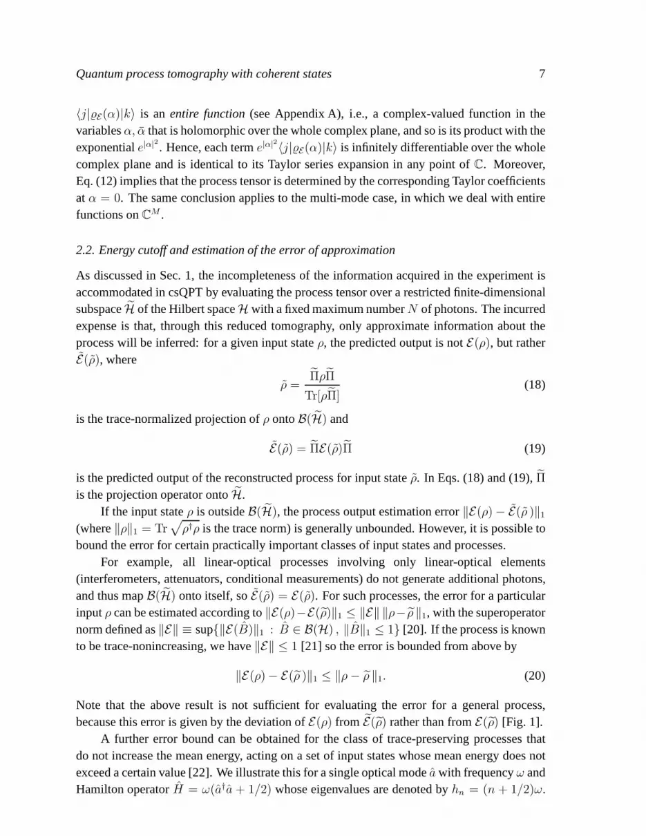
Note that the above result is not sufficient for evaluating the error for a general process,because this error is given by the deviation ofE(ρ) from E(ρ) rather than fromE(ρ) [Fig. 1].

A further error bound can be obtained for the class of trace-preserving processes thatdo not increase the mean energy, acting on a set of input states whose mean energy does notexceed a certain value [22]. We illustrate this for a single optical modea with frequencyω andHamilton operatorH = ω(a†a + 1/2) whose eigenvalues are denoted byhn = (n + 1/2)ω.


!~

)( E

)~( E

)~(~ E

)(HB

)(HB

)~

(HB )~

(HB

Figure 1. Errors associated with photon number cutoff. RestrictingB(H) to B(H) results inapproximationρ of the input stateρ. If the error of this approximation‖ρ − ρ ‖1 is known,the error of the images‖E(ρ)− E(ρ )‖1 can be estimated according to Eq. (20). However, thedifference betweenE(ρ) andE(ρ) in the cutoff space remains generally unknown.

Suppose that the quantum statesρ of interest satisfyTr[ρH ] ≤ U . According to Ref. [22], ifwe choose the cutoff dimensiondim(H) = N + 1 such thatU/hN+1 ≤ γ for some (small)γ > 0, the reconstructed process output errors are bounded from above as

∥∥∥∥∥E(ρ)−E(ρ)

Tr E(ρ)

∥∥∥∥∥1

≤ 2ǫ, (21)

whereǫ = 2

√γ + γ/(1− γ). (22)

Conversely, if we want to achieve a certain upper boundǫ on the error of approximation(which corresponds to a lower bound on the desired accuracy of the process characterization),we first solve Eq. (22) forγ = γ(ǫ), and then find the minimumNγ ∈ N such thatU/hNγ+1 ≤ γ. Any cutoff dimensionN + 1 > Nγ is then sufficient for our purpose. Forγ ≪ 1, ǫ ≈ 2

√γ, which yields

ǫ = O(1/√N). (23)

This implies that the error of approximation scales as1/√N with the cutoff dimensionN+1.

For example, in order to achieve a 10% error in Eq. (21), we need ǫ = 0.05 and thusγ ≈ 0.0006. For the input mean energy bound corresponding to one photon(U = 3/2ω), therequired cutoff isN ≈ U/γ ≈ 250. This calculation shows that the above error estimate isextremely conservative.

3. Phase-invariant processes

Many practically relevant processes, including the single-mode processes studied in Sec. 4,exhibit phase invariance. If two input states are identicalup to a shift by an optical phaseφ,


the process outputs for these states differ by the same phaseshift:

E [einφρe−inφ] = einφE(ρ)e−inφ. (24)

For such processes, it is convenient to express the probe coherent states in polar coordinates:|α〉 =

∣∣reiθ⟩= einθ |r〉. Specifically, in these coordinates, we have [9]

Pmn(r, θ) =

√m!n!

(m+ n)!er

2+iθ(n−m)(−1)m+n dm+n

drm+nδ(r), (25)

and accordingly

Emnjk =

√m!n!

(m+ n)!

dm+n

drm+n

[∫ 2π

0

dθ2π

er2+iθ(n−m) 〈j| E(r, θ) |k〉

] ∣∣∣∣r=0

. (26)

Hence Eq. (24) can be expressed as

〈j| E(|α〉〈α|) |k〉 = eiθ(j−k) 〈j| E(|r〉〈r|) |k〉 , (27)

and the superoperatorE [Eq. (26)] has the following explicit representation:

Emnjk =

√m!n!

(m+ n)!

dm+n

drm+n

[er

2 〈j| E(|r〉〈r|) |k〉] ∣∣∣∣

r=0

δm−j,n−k. (28)

In experimental tomography of phase-invariant processes [7, 12], it is sufficient tomeasure the process output for a discrete set of coherent states{|ri〉} on the real axis of thephase space. The matrix elements of the output states can then be interpolated as polynomialfunctions

〈j| E(|r〉〈r|) |k〉 =Q∑

l=0

Cl(j, k)rl, (29)

whereQ is the degree of the polynomial (which depends on the dimension of the truncatedHilbert space) andCl(j, k) are its coefficients. Furthermore, from Eq. (A.3) together withEq. (28), it follows that, for phase-symmetric processes, when j − k is even or odd,〈j| E(|r〉〈r|) |k〉 and its analytic extension to negative values ofr are even or odd functionsof r, respectively. By taking into account the symmetric or antisymmetric property of thisfunction, we have additional information to be used in the interpolation procedure; theconstructed polynomial has to contain only even or odd powers of r, respectively. In thisway the precision of process estimation from the experimental data is substantially increased.

With the knowledge of the coefficientsCl(j, k), Eq. (28) is further simplified to:

Emnjk =

√m!n!

(m+ n)!

dm+n

drm+n

[∞∑

s=0

r2s

s!

Q∑

l=0

Cl(j, k)rl

] ∣∣∣∣∣r=0

δm−j,n−k

=

√m!n!

(m+ n)!

∞∑

s=0

Q∑

l=0

δm+n,2s+l(m+ n)!

s!Cl(j, k)δm−j,n−k

=√m!n!

⌊(m+n)⌋/2∑

s=0

Cm+n−2s(j, k)

s!δm−j,n−k . (30)


The last result is significant in that one can obtain the process tensor directly from theexperimentally reconstructed output states through simple summation. Moreover, if thedimension of the truncated Hilbert space isd = N + 1, from Eq. (30) it follows that onlyterms of powerl ≤ 2N of the interpolation polynomial (29) contribute to the process tensor.We have tested this procedure on experimental data [12] and calculated the process tensor in afew microseconds, which is a dramatic improvement in comparison to several hours requiredfor the original procedure [7, 12].

4. Examples: superoperators of important quantum optical processes

In this section, we illustrate our new method by applying it to some fundamental quantumoptical processes, whose effects on coherent states are known. Specifically, using Eqs. (12) or(16), we analytically derive corresponding superoperatortensorsEmn

jk in the Fock basis. Theresults are summarized in Table 1.

4.1. Identity

For the identity process (Eid), Eid(α) = |α〉〈α|, the matrix elements of the output states are

〈j| Eid(α) |k〉 = e−|α|2 αjαk

√j!k!

. (31)

Inserting these elements into Eq. (12) yieldsEmnjk = δmjδnk, as expected.

4.2. Attenuation and lossy channel

For attenuation of light fields (Eatt), the process’s effect on single-mode coherent states is givenby Eatt(α) = |ηα〉〈ηα|, where0 ≤ η < 1. The matrix elements in the Fock basis are

〈j| Eatt(α) |k〉 = e−η2|α|2 ηj+kαjαk

√j!k!

. (32)

From Eq. (12), we obtain

Emnjk =

ηj+k

√m!n!j!k!

∂mα ∂n

α

[e|α|

2(1−η2)αjαk] ∣∣∣

α,α=0

=ηj+k

√m!n!j!k!

∂mα ∂n

α

∞∑

l=0

(1− η2)lαj+lαk+l

l!

∣∣∣α,α=0

=

√m!n!

j!k!

ηj+k(1− η2)m−j

(m− j)!δm−j,n−k , (33)

which depends explicitly onη.


a)

b)

single-photon

detector low-reflectivity

beam splitter

idler

signalparametric

down-conversion

pump

beam

†ˆˆ aa

aa ˆˆ†

Figure 2. Experimental realizations of (a) photon subtraction and (b) photon addition. Theprocess is heralded by single-photon detection events.

4.3. Photon subtraction and addition

Photon subtraction is defined as a process that removes a single photon from the lightfield, whereas photon addition adds a single photon. Photon subtraction has been used byOurjoumtsev et al. [23] to generate optical Schrodinger kittens (coherent superpositions oflow-amplitude coherent states) from squeezed vacuum states for the purpose of quantuminformation processing. Single-photon-added coherent states can be regarded as the resultof the most elementary amplification process of classical light fields by a single quantum ofexcitation; being intermediate between single-photon Fock states (fully quantum-mechanical)and coherent (classical) ones, these states have been demonstrated to be suited for the studyof smooth transition between the particle-like and the wavelike behavior of light [24].

Here we discuss idealized single-mode photon subtraction and photon addition. Bothprocesses are non-trace-preserving. For example, photon subtraction can be approximatelyrealized [23] by a highly-transmissive beam splitter, whose reflected mode is directed to adetector and whose transmitted mode constitutes the output, respectively, as illustrated inFig. 2a. Any click in a detector implies extraction of photon(s) from the input mode bythe beam splitter. As the beam splitter has low reflectivity,here single-photon extractionevents are more likely than multi-photon events. An approximate experimental realization ofphoton addition is illustrated in Fig. 2b. The input quantumstateρ enters the signal channelof a parametric down-conversion setup. Provided that detector dark counts are neglected, aphoton detection in the idler mode heralds photon addition to the signal mode, which containsthe output state of the process.

The effect of photon subtraction (Esub) and addition (Eadd) on coherent states is given byEsub(α) = a|α〉〈α|a† andEadd(α) = a†|α〉〈α|a, respectively, wherea and a† are the photonannihilation and photon creation operators of a single mode, respectively. The matrix elements


of the output states in the Fock basis are

〈j| Esub(α) |k〉 = e−|α|2αj+1αk+1

√j!k!

, (34)

〈j| Eadd(α) |k〉 = e−|α|2√kj

αj−1αk−1

√(j − 1)!(k − 1)!

. (35)

The process tensor is found to be

Emnjk =

{ √(j + 1)(k + 1)δm,j+1δn,k+1, for photon subtraction,√kjδm,j−1δn,k−1, for photon addition,

(36)

where we have employed Eq. (12).

4.4. Schrodinger cat generation

The unitary evolution according toUKerr(χ) ≡ exp[−iχ

(a†a

)2]for χ = π/2, if applied to

coherent states, generates Schrodinger cat states (hereafter denoted asEcat) [25, 26]

Ecat(α) = UKerr(π

2) |α〉〈α| U †

Kerr(π

2)

=1

2(|α〉+ i |−α〉)(〈α| − i 〈−α|), (37)

with matrix elements

〈j| Ecat(α) |k〉 =e−|α|2αjαk

2√j!k!

[1 + (−1)j+k + i(−1)j − i(−1)k

]. (38)

The superoperator tensor for this non-Gaussian unitary process obtained via Eq. (12) is

Emnjk = e−iπ

2(j2−k2)δmjδnk . (39)

Interestingly, this process does not change the total particle number of any input state.

4.5. Beam splitter

Now let us consider the beam splitter as an example of a two-mode process. The unitary beamsplitter transformation is given by [27]

B(Θ) = eΘ

2(a†

2a1−a†

1a2), (40)

whereΘ is the parameter identifying how the beam splitter transmits or reflects beams.Specifically, its action on coherent state inputs|α1〉 and|α2〉 is given as

EB(α1, α2) =EB(|α1, α2〉〈α1, α2|)

=B†(Θ)(|α1, α2〉〈α1, α2|)B(Θ)

=|Tα1 −Rα2, Rα1 + Tα2〉〈Tα1 − Rα2, Rα1 + Tα2|, (41)


with T ≡ cos(Θ/2) and R ≡ sin(−Θ/2) being the transmissivity and reflectivity,respectively. By knowing the effect of the process on two-mode coherent states, we cancalculate the corresponding tensor using Eq. (16), which yields

Em1m2n1n2

j1j2k1k2=

√m1!m2!n1!n2!

j1!j2!k1!k2!

j1∑

p=0

k1∑

q=0

(j1p

)(j2

m1 − p

)(k1q

)

×(

k2n1 − q

)T 2p+2q+j2+k2−m1−n1

× (−1)j1+k1−p−qRj1+k1+m1+n1−2p−2q

× δm1+m2,j1+j2δn1+n2,k1+k2, (42)

as an explicit function ofT andR.

4.6. Parametric down-conversion

Another two-mode process of interest is parametric down-conversion (PDC). In PDC, a crystalwith an appreciably large second-order non-linearity is pumped by a laser field. Each ofthe pump photons can spontaneously decay into a pair of identical (degenerate PDC) ornonidentical photons (nondegenerate PDC). Here we consider a nondegenerate PDC processEPDC induced by the transformation [27]

S2(r) = er(a1a2−a†1a†2). (43)

The effect of this unitary process on a two-mode coherent state is given by

EPDC(α1, α2) = EPDC(|α1, α2〉〈α1, α2|)= S2(r) |α1, α2〉〈α1, α2| S†

2(r). (44)

In Appendix B, we derive the process tensor in the Fock basis.The result can be expressedas:

Em1m2n1n2

j1j2k1k2=

√n1!m1!m2!n2!

j1!k1!k2!j2!

(tanh r)m1+n1−j1−k1

(m1 − j1)! (n1 − k1)! (cosh r)j2+k2−j1−k1+2

× 2F1

(−j1, m2 + 1;m1 − j1 + 1; tanh2 r

)

× 2F1

(−k1, n2 + 1;n1 − k1 + 1; tanh2 r

)

× δm2−m1,j2−j1 δn2−n1,k2−k1 , (45)

with

2F1(α, β; γ; z) := 1 +

∞∑

n=1

(α)n(β)n(γ)n

zn

n!, (46)

the hypergeometric function,(x)n := Γ(x + n)/Γ(x) the Pochhammer symbol andΓ(·) theGamma function [28].


Table 1. Process tensorEmnjk for some quantum optical processes.

OperationE E(α) Process tensorEmnjk

Identity (Eid) |α〉〈α| δmjδnk

Attenuation (Eatt) |ηα〉〈ηα|√

m!n!j!k!

ηj+k(1−η2)m−j

(m−j)! δm−j,n−k

Photon addition (Eadd) a†|α〉〈α|a√kjδm,j−1δn,k−1

Photon subtraction (Esub) a|α〉〈α|a†√(j + 1)(k + 1)δm,j+1δn,k+1

Cat generation (Ecat) 12 (|α〉+ i |−α〉) e−iπ

2(j2−k2)δmjδnk

×(〈α| − i 〈−α|)

Beam splitter (EB) |Tα1 −Rα2, Rα1 + Tα2〉√

m1!m2!n1!n2!j1!j2!k1!k2!

∑j1p=0

∑k1

q=0(−1)j1+k1−p−q

×〈Tα1 −Rα2, Rα1 + Tα2| ×(j1p

)(j2

m1−p

)(k1

q

)(k2

n1−q

)

×T 2p+2q+j2+k2−m1−n1

×Rj1+k1+m1+n1−2p−2q

×δm1+m2,j1+j2δn1+n2,k1+k2

Parametric down- er(a1a2−a†1a†2) |α1, α2〉

√m1!m2!n1!n2!j1!j2!k1!k2!

conversion (EPDC) ×〈α1, α2| er(a†1a†2−a1a2) × (tanh r)m1+n1−j1−k1

(m1−j1)! (n1−k1)! (cosh r)j2+k2−j1−k1+2

× 2F1

(−j1,m2 + 1;m1 − j1 + 1; tanh2 r

)

× 2F1

(−k1, n2 + 1;n1 − k1 + 1; tanh2 r

)

× δm2−m1,j2−j1δn2−n1,k2−k1

5. Conclusions

Coherent states are easily generated probe states for tomography of unknown quantum-optical processes. Here, we have presented a new, more efficient data processing techniquefor estimating a quantum process from similar experimentalprocedure of Ref. [7]. Theoriginal formulation was based on regularization and filtering of the Glauber-Sudarshanrepresentations for quantum states, which are cumbersome to implement numerically.Furthermore, Ref. [7] introduces additional errors associated with regularization of thePfunction. In contrast, our new method to determine the process superoperator [Eq. (12) orEq. (16)] is mathematically simpler, computationally faster and unique up to the choice ofthe energy cutoff. Moreover, we presented straightforwardgeneralizations of coherent statequantum process tomography to multi-mode and non-trace-preserving conditional processes.

We have illustrated the new framework through several examples (summarized inTable 1). We have shown that it is straightforward to derive analytically exact and uniqueclosed-form expressions for the superoperators for quantum optical processes whose effect


on coherent states is known. For phase-invariant unknown processes, the formula to find theprocess tensor reduces to a simple summation of coefficientsof a polynomial obtained fromthe experimentally reconstructed output states via interpolation.

An interesting consequence implied by our formulation [in particular, Eqs. (12) and (16)]is that complete information about a quantum optical process is entirely captured by its effecton a compact set of all coherent states|α〉 in the immediate vicinity of the vacuum state.This is due to the entireness property of the image of processes on coherent states. It thusappears sufficient to perform tomography experiments only for a range of coherent stateswhose mean photon number is much smaller than that required for the method of Ref. [7] (seethe suppl. material therein). However, coherent state quantum process tomography relies onthe ability to approximately determine all the derivativesof a function which is obtained byinterpolation from measured experimental data. Minimization of errors associated with thiscalculation imposes a lower bound on the phase space region over which the measurementsneed to be performed. For the time being, we have provided an evaluation of the error in theprocess estimation by introducing a truncation of the Fock space. For the class of processesrespecting a certain energy constraint (which includes allprocesses that do not amplify theenergy), we have determined (i) the cutoff dimension that issufficient in order to achievea certain degree of approximation accuracy, as well as (ii) the upper bound on the error ofestimation for a given cutoff dimension.

Acknowledgments:We acknowledge financial support by NSERC,iCORE, MITACS, QuantumWorks and

General Dynamics Canada. AIL is a CIFAR Scholar, and BCS is a CIFAR Fellow. We wouldalso like to thank Connor Kupchak for helpful discussions.

Appendix A. Proof that 〈j| E(α) |k〉 is an entire function

According to Eq. (12), by knowing the complex-valued function 〈j| E(α) |k〉 (of the variableα) for anyj andk, one can determine the process tensorEmn

jk . Here we show that this functionis anentire functionso it can be represented as a power series that converges uniformly onany compact domain.

As a completely-positive quantum operation,E possesses a Kraus decompositionE(ρ) =∑Li=1 Ki ρ K

†i , whereL ≤ dim(H)2 andKi are some Kraus operators onH (whose explicit

form is not needed for our purpose). Hence we can rewrite the matrix elements of the outputstate as

〈j| E(α) |k〉 =L∑

i=1

〈j| Ki |α〉〈α| K†i |k〉

=

L∑

i=1

〈α| K†i |k〉〈j| Ki |α〉

= 〈α| E∗(|k〉〈j|) |α〉 , (A.1)


where

E∗ : B(H) → B(H) , B 7→L∑

i=1

K†i B Ki, (A.2)

is the dual or adjoint map [29]. The complex-valued function〈α| A |α〉 (referred to as Husimifunction if A is a density operator)—whereA is any bounded operator onH—is an entirefunction of the two variablesα andα [13, 30]. Hence the right hand side of Eq. (A.1) impliesthat the function〈j| E(α) |k〉 is an entire function. By representing the coherent states inEq. (A.1) in the Fock basis and using Eq. (6), we obtain

〈j| E(α) |k〉 = e−|α|2∞∑

n=0

∞∑

m=0

αnαm

√n!m!

Enmjk , (A.3)

which is a power series of the complex variablesα and α, hence convergent everywhere[13, 30].

Appendix B. Process tensor for parametric down-conversion

To obtain the Fock representation of the PDC process, we firstfind the matrix elements of theoutput states in the Fock basis:

〈j1, j2| EPDC(α1, α2) |k1, k2〉 = 〈j1, j2| S2(r) |α1, α2〉〈α1, α2| S†2(r) |k1, k2〉

= I × J , (B.1)

whereI := 〈α1, α2| S†2(r) |k1, k2〉 andJ := 〈α1, α2| S†

2(r) |j1, j2〉. Employing the relations

S†2(r) |0, 0〉 =

1

cosh r

∞∑

l=0

(tanh r)l |l, l〉 , (B.2)

S†2(r)a1S2(r) = a1 cosh r − a†2 sinh r, (B.3)

S†2(r)a2S2(r) = a2 cosh r − a†1 sinh r, (B.4)

and the binomial expansion, we have:

I = 〈α1, α2| S†2(r)

(a†1)k1

√k1!

(a†2)k2

√k2!

S2(r)S†2(r) |0, 0〉

=1

cosh r√k1!k2!

∞∑

l=0

(tanh r)l 〈α1α2|k1∑

p=0

(k1p

)(a†1 cosh r)

k1−p(−a2 sinh r)p

×k2∑

q=0

(k2q

)(a†2 cosh r)

k2−q(−a1 sinh r)q |l, l〉 . (B.5)


Usingax |l〉 =√

l!/(l − x)! |l − x〉 and(a†)y |l〉 =√

(l + y)!/l! |l + y〉 we obtain:

I =1

cosh r√k1!k2!

∞∑

l=0

(tanh r)lk1∑

p=0

(k1p

)(cosh r)k1−p(− sinh r)p

×k2∑

q=0

(k2q

)(cosh r)k2−q(− sinh r)qe−|α1|2/2−|α2|2/2

× αl+k1−q−p1 αl+k2−q−p

2

(l + k2 − q)!

(l − q)!(l + k2 − q − p)!. (B.6)

From the symmetry betweenI andJ , and by replacingk1 andk2 by j1 andj2, respectively,we also find:

J =1

cosh r√j1!j2!

∞∑

l′=0

(tanh r)l′

j1∑

u=0

(j1u

)(cosh r)j1−u(− sinh r)u

×j2∑

v=0

(j2v

)(cosh r)j2−v(− sinh r)v e−|α1|2/2−|α2|2/2

× αl′+j1−u−v1 αl′+j2−u−v

2

(l′ + j2 − v)!

(l′ − v)! (l′ + j2 − u− v)!. (B.7)

The Fock representation of the superoperator for the PDC process is then given by

Em1m2n1n2

j1j2k1k2=

1√m1!m2!n1!n2!

∂m1

α1∂n1

α1∂m2

α2∂n2

α2

(e|α1|2+|α2|2I × J

) ∣∣∣∣α1,α2=0

=

√n1!m1!

n2!m2!

1

cosh r2√j1!j2!k1!k2!

k1∑

p=0

(k1p

)(cosh r)k1−p(− sinh r)p

× (tanh r)n1−k1+p (n1 − k1 + k2 + p)!

(n1 − k1 + p)!δn1−n2,k2−k2

×k2∑

q=0

(k2q

)(cosh r)k2−q(− sinh r tanh r)q

×j1∑

u=0

(j1u

)(cosh r)j1−u(− sinh r)u(tanh r)m1−j1+u (m1 − j1 + j2 + u)!

(m1 − j1 + u)!

× δm2−m1,j2−j1

j2∑

v=0

(j2v

)(cosh r)j2−v(− sinh r tanh r)v

=

√n1!m1!k1!j1!

n2!m2!k2!j2!

(tanh r)n1+m1

(cosh r)k2+j2+2

×k1∑

p=0

j1∑

u=0

( cosh rtanh r

)k1+j1−p−u (− sinh r)p+u

p! (k1 − p)! u! (j1 − u)!

× (n2 + p)! (m2 + u)!

(n1 − k1 + p)! (m1 − j1 + u)!δn2−n1,k2−k1 δm2−m1,j2−j1 , (B.8)


which can also be expressed in terms of a product of values of the hypergeometric function

2F1, as given by Eq. (45).

References

[1] J. F. Poyatos, J. I. Cirac, and P. Zoller, Phys. Rev. Lett.78, 390 (1997).[2] G. M. D’Ariano and P. Lo Presti, Phys. Rev. Lett.86, 4195 (2001).[3] M. Mohseni, A. T. Rezakhani, and D. A. Lidar, Phys. Rev. A77, 032322 (2008).[4] J. L. O’Brien, G. J. Pryde, A. Gilchrist, D. F. V. James, N.K. Langford, T. C. Ralph, and A. G. White,

Phys. Rev. Lett.93, 080502 (2004).[5] A. M. Childs, I. L. Chuang, and D. W. Lueng, Phys. Rev. A64, 012314 (2001).[6] M. W. Mitchell, C. W. Ellenor, S. Schneider, and A. M. Steinberg, Phys. Rev. Lett.91, 120402 (2003).[7] M. Lobino, D. Korystov, C. Kupchak, E. Figueroa, B. C. Sanders, and A. I. Lvovsky, Science322, 563

(2008).[8] R. J. Glauber, Phys. Rev. Lett.10, 84 (1963).[9] E. C. G. Sudarshan, Phys. Rev. Lett.10, 277 (1963).

[10] We adopt[x, p] = i for the position and momentum quadratures [~ ≡ 1], whenceα = (x+ ip)/√2.

[11] A. I. Lvovsky and M. G. Raymer, Rev. Mod. Phys.81, 299 (2009).[12] M. Lobino, C. Kupchak, E. Figueroa, and A. I. Lvovsky, Phys. Rev. Lett.102, 203601 (2009).[13] K. E. Cahill, Phys. Rev.138, B1566 (1965).[14] K. E. Cahill, Phys. Rev.180, 1239 (1969).[15] J. R. Klauder, Phys. Rev. Lett.16, 534 (1966).[16] I. M. Gel’fand and G. E. Shilov,Generalized Functions, Vol. 1(Academic Press, New York, 1964).[17] E. Knill, R. Laflamme, and G. J. Milburn, Nature409, 46 (2001).[18] K. E. Cahill, Phys. Rev.180, 1244 (1969).[19] J. F. Scherson, H. Krauter, R. K. Olsson, B. Julsgaard, K. Hammerer, I. Cirac, and E. S. Polzik, Nature443,

557 (2006).[20] A. Yu. Kitaev, Russ. Math. Surv.52, 1191 (1997).[21] M. A. Nielsen and I. L. Chuang,Quantum Computation and Quantum Information(Cambridge University

Press, Cambridge, England, 2000).[22] G. M. D’Ariano, D. Kretschmann, D. Schlingemann, and R.F. Werner, Phys. Rev. A76, 032328 (2007).[23] A. Ourjoumtsev, R. Tualle-Brouri, J. Laurat, and P. Grangier, Science312, 83 (2006).[24] A. Zavatta, S. Viciani, and M. Bellini, Science306, 660 (2004).[25] G. J. Milburn, Phys. Rev. A33, 674 (1986).[26] B. Yurke and D. Stoler, Phys. Rev. Let.57, 13 (1986).[27] B. Yurke, S. L. McCall, and J. R. Klauder, Phys. Rev. A33, 4033 (1986).[28] M. Abramowitz and I. A. Stegun,Handbook of Mathematical Functions with Formulas, Graphs,and

Mathematical Tables(Dover, New York, 1972).[29] D. Kretschmann, D. Schlingemann, and R. F. Werner, IEEETrans. Inf. Theory54, 1708 (2008).[30] L. Mandel and E. Wolf,Optical Coherence and Quantum Optics(Cambridge University Press, New York,

1995).

Quantum process tomography with coherent states

Documents

Transcript of Quantum process tomography with coherent states