Learning vector quantization for (dis-)similarities

Barbara Hammer, Daniela Hofmann, Frank-Michael Schleif, Xibin Zhu

CITEC center of excellence, Bielefeld University, Germany

March 5, 2013

Abstract

Prototype-based methods often display very intuitive classificationand learning rules. However, popular prototype based classifiers suchas learning vector quantization (LVQ) are restricted to vectorial dataonly. In this contribution, we discuss techniques how to extend LVQalgorithms to more general data characterized by pairwise similaritiesor dissimilarities only. We propose a general framework how the meth-ods can be combined based on the background of a pseudo-Euclideanembedding of the data. This covers the existing approaches kernelgeneralized relevance LVQ and relational generalized relevance LVQ,and it opens the way towards two novel approach, kernel robust softLVQ and relational robust soft LVQ. Interestingly, also unsupervisedprototype based techniques which are based on a cost function canbe put into this framework including kernel and relational neural gasand kernel and relational self-organizing maps (based on Heskes’ costfunction). We demonstrate the performance of the LVQ techniques forsimilarity or dissimilarity data in several benchmarks, reaching stateof the art results.

1 Introduction

Since electronic data sets increase rapidly with respect to size and com-plexity, humans have to rely on automated methods to access relevant in-formation from such data. Apart from classical statistical tools, machinelearning has become a major technique in the context of data processingsince it offers a wide variety of inference methods. Today, a major part ofapplications is concerned with the inference of a function or classificationprescription based on a given set of examples, accompanied by data miningtasks in unsupervised machine learning scenarios and more general settings

1

as tackled e.g. in the frame of autonomous learning. In this contribution,we focus on classification problems.

There exist many different classification techniques in the context ofmachine learning ranging from symbolic methods such as decision trees tostatistical methods such as Bayes classifiers. Because of its often excellentclassification and generalization performance, the support vector machine(SVM) constitutes one of the current flagships in this context, having itsroots in learning theoretical principles as introduced by Vapnik and col-leagues [4]. Due to its inherent regularization of the result, it is particularlysuited if high dimensional data are dealt with. Further, the interface to thedata is given by a kernel matrix such that, rather than relying on vectorialrepresentations, the availability of the Gram matrix is sufficient to applythis technique.

With machine learning techniques becoming more and more popular indiverse application domains and the tasks becoming more and more complex,there is an increasing need for models which can easily be interpreted bypractitioners: for complex tasks, often, practitioners do not only apply amachine learning technique but also inspect and interpret the result suchthat a specification of the tackled problem or an improvement of the modelbecomes possible [40]. In this setting, a severe drawback of many state-of-the-art machine learning tools such as the SVM occurs: they act as black-boxes. In consequence, practitioners cannot easily inspect the results and itis hardly possible to change the functionality or assumptions of the modelbased on the result of the classifier.

Prototype-based methods enjoy a wide popularity in various applicationdomains due to their very intuitive and simple behavior: they represent theirdecisions in terms of typical representatives contained in the input spaceand a classification is based on the distance of data as compared to theseprototypes [19]. Thus, models can be directly inspected by experts sinceprototypes can be treated in the same way as data. Popular techniques inthis context include standard learning vector quantization (LVQ) schemesand extensions to more powerful settings such as variants based on costfunctions or metric learners such as robust soft LVQ (RSLVQ) or generalizedLVQ (GLVQ), for example [32, 37, 38, 36]. These approaches are based onthe notion of margin optimization similar to SVM in case of GLVQ [37], orbased on a likelihood ratio maximization in case of RSLVQ, respectively [38].For GLVQ and RSLVQ, a behavior which closely resembles standard LVQ2.1results in limit cases. The limit case of RSLVQ does not necessarily achieveoptimum behavior already in simple model situations similar to LVQ2.1,as has been investigated in the context of the theory of online learning

2

[2]. Nevertheless, it displays excellent generalization ability in the standardintermediate case, see e.g. [36] for an extensive comparison of the techniques.

With data sets becoming more and more complex, input data are oftenno longer given as simple Euclidean vectors, rather structured data or ded-icated formats can be observed such as sequences, graphs, tree structures,time series data, functional data, relational data etc. as occurs in bioinfor-matics, linguistics, or diverse heterogeneous databases. Several techniquesextend statistical machine learning tools towards non-vectorial data: kernelmethods such as SVM using structure kernels, recursive and graph networks,functional methods, relational approaches, and similar [9, 33, 11, 31, 14].

Recently, popular prototype-based algorithms have also been extendedto deal with more general data. Several techniques rely on a characterizationof the data by means of a matrix of pairwise similarities or dissimilaritiesonly rather than explicit feature vectors. In this setting, median clusteringas provided by median self-organizing maps, median neural gas, or affinitypropagation characterizes clusters in terms of typical exemplars [10, 20, 8].More general smooth adaptation is offered by relational extensions suchas relational neural gas or relational learning vector quantization [13]. Afurther possibility is offered by kernelization such as proposed for neural gas,self-organizing maps, or different variants of learning vector quantization[29, 41, 30]. By formalizing the interface to the data as a general similarity ordissimilarity matrix, complex structures can be easily dealt with: structurekernels for graphs, trees, alignment distances, string distances, etc. open theway towards these general data structures [27, 11].

In this contribution, we consider the question how to extend cost func-tion based LVQ variants such as RSLVQ (11) or GLVQ (2) to similarityor dissimilarity data, respectively. We propose a general way based on animplicit pseudo-Euclidean embedding of the data, and we discuss in how farinstantiations of this framework differ from each other. Using this frame-work, we cover existing techniques such as kernel GLVQ [30] and relationalGLVQ [15], and investigate novel possibilities such as kernel and relationalRSLVQ. These techniques offer valid classifiers and training methods for anarbitrary symmetric similarity or dissimilarity. Some mathematical proper-ties, however, such as an interpretation via a likelihood ratio or interpre-tation of learning as exact gradient, are only guaranteed in the Euclideancase for some of the possible choices, as we will discuss in this article. Inthis context, we investigate the effect of corrections of the matrix to makedata Euclidean. The effectivity of the novel techniques is demonstrated ina couple of benchmarks.

Now, we first introduce standard LVQ for Euclidean vectors, in partic-

3

ular the two cost-function based variants GLVQ and RSLVQ. Afterwards,we review facts about similarity and dissimilarity data and their pseudo-Euclidean embedding. Based on this embedding, kernel and relational vari-ants of LVQ can be introduced for similarities or dissimilarities, respectively.Training can take place essentially in two ways, mimicking the correspond-ing Euclidean counterparts or via direct gradients, respectively, whereby thesame local optima of the cost function are present in the Euclidean case, buta numerical scaling of the gradients is observed. We exemplarily derive newmodels, kernel RSLVQ and relational RSLVQ in this framework. Experi-ments are based on the setting as proposed in [6], investigating the effectof different preprocessing steps and learning techniques in comparison tothe results of SVM and a k-nearest neighbor classifier. We conclude with adiscussion.

2 Learning vector quantization

Learning vector quantization (LVQ) constitutes a very popular class of intu-itive prototype based learning algorithms with successful applications rang-ing from telecommunications to robotics [19]. Basic algorithms as proposedby Kohonen include LVQ1 which is directly based on Hebbian learning,and improvements such as LVQ2.1, LVQ3, or OLVQ which aim at a higherconvergence speed or better approximation of the Bayesian borders. Thesetypes of LVQ schemes have in common that their learning rule is essentiallyheuristically motivated and a valid cost function does not exist [3]. Oneof the first attempts to derive LVQ from a cost function can be found in[32] with an exact computation of the validity at class boundaries in [36].Later, a very elegant LVQ scheme which is based on a probabilistic modeland which can be seen as a more robust probabilistic extension of LVQ2.1has been proposed in [38]. We shortly review these two proposals.

2.1 Generalized learning vector quantization

Assume data ξi ∈ Rn with i = 1, . . . , N are labeled yi where labels stem from

a finite number of different classes. A GLVQ network is characterized bym prototypes wj ∈ R

n with priorly fixed labels c(wj). Classification takesplace by a winner takes all scheme:

ξ 7→ c(wj) where d(ξ, wj) is minimum (1)

with squared Euclidean distance d(ξ, wj) = ‖ξ − wj‖2, breaking ties arbi-

trarily.

4

For training, it is usually assumed that the number and classes of pro-totypes are fixed. In practice, these are often determined using cross-validation, or a further wrapper technique is added to obtain model flex-ibility. Training aims at finding positions of the prototypes such that theclassification accuracy of the training set is optimized. GLVQ also takes thegeneralization ability into account, using the costs

∑

i

d(ξi, w+)− d(ξi, w

−)

d(ξi, w+) + d(ξi, w−)(2)

where w+ constitutes the closest prototype with the same label as ξi and w−

constitutes the closest prototype with a different label than ξi. The nomi-nator is negative iff ξi is classified correctly, thus GLVQ tries to maximizethe number of correct classifications. In addition, it aims at an optimiza-tion of the hypothesis margin d(ξi, w

−) − d(ξi, w+) which determines the

generalization ability of the method [37].Training takes place by a simple stochastic gradient descent, i.e. given a

data point ξi, adaptation takes place via

∆w+ ∼ −2 · d(ξi, w

−)

(d(ξi, w+) + d(ξi, w−))2·∂d(ξi, w

+)

∂w+(3)

∆w− ∼2 · d(ξi, w

+)

(d(ξi, w+) + d(ξi, w−))2·∂d(ξi, w

−)

∂w−(4)

From an abstract point of view, we can characterize GLVQ as a classifier,which classification rule is based on a number of quantities

D(ξ, w) := (d(ξi, wj))i=1,...,N,j=1,...,m (5)

Training aims at an optimization of a cost function of the form

f(D(ξ, w)) (6)

by means of the gradients

∂f(D(ξ, w))

∂wj=

m∑

i=1

∂f(D(ξ, w))

∂d(ξi, wj)·∂d(ξi, wj)

∂wj(7)

with respect to the prototypes wj or the corresponding stochastic gradientsfor one point ξi.

5

2.2 Robust soft learning vector quantization

Robust soft LVQ (RSLVQ) models data by a mixture of Gaussians andderives learning rules as a maximization of the log likelihood ratio of thegiven data. In the limit of small bandwidth σ, a learning rule which issimilar to LVQ2.1 but which performs adaptation in case of misclassificationonly, is obtained [38].

Here, we restrict to the standard model which assumes equal prior andbandwidth of the modes. Mixture component j defines the probability

p(ξ|j) = (2πσ2)−n/2 · exp(−d(ξ, wj)/σ2) (8)

This induces the probability of an unlabeled data point

p(ξ|W ) =1

m·∑

j

p(ξ|j) (9)

with parameters W of the model. The probability of a labeled data point is

p(ξ, y|W ) =1

m·

∑

j : c(wj)=y

p(ξ|j) . (10)

Learning aims at an optimization of the log likelihood ratio

L =∑

i

logp(ξi, yi|W )

p(ξi|W ). (11)

A stochastic gradient ascent yields the following update rules, given datapoint ξi with label yi:

∆wj ∼

{

−(Py(j|ξi)− P (j|ξi)) · ∂d(ξi, wj)/∂wj if c(wj) = yiP (j|ξi) · ∂d(ξi, wj)/∂wj if c(wj) 6= yk

(12)

with the probabilities

Py(j|ξi) =exp(−d(ξi, wj)/σ

2)∑

j:c(wj)=yiexp(−d(ξi, wj)/σ2)

(13)

and

P (j|ξi) =exp(−d(ξi, wj)/σ

2)∑

j exp(−d(ξi, wj)/σ2))(14)

With small bandwidth, a learning rule similar to LVQ2.1, learning frommistakes, results thereof.

6

Given a novel data point ξ, its class label can be determined by meansof the most likely label y corresponding to a maximum value p(y|ξ,W ) ∼p(ξ, y|W ). For typical settings, this rule can usually be approximated by asimple winner takes all rule as in GLVQ (1). It has been shown in [38], forexample, that RSLVQ often yields excellent results while preserving inter-pretability of the model due to prototypical representatives of the classes interms of the parameters wj .

Note that the objective of RSLVQ and GLVQ training is in both casesa function of the form f(D(ξ, w)). Similarly, the classification depends onthe vector D(ξ, w) only.

3 Extensions to dis-/similarity data

In modern applications, data are often no longer vectorial. Rather, complexstructures are dealt with for which a problem specific similarity or dissim-ilarity measure has been designed. Examples include biological sequences,mass spectra, or metabolic networks, where complex alignment techniques,background information, or general information theoretical principles, forexample, drive the comparison of data points [28, 22, 18]. In these settings,it is possible to compute pairwise similarities or dissimilarities of the datarather than to arrive at an explicit vectorial representation.

The question occurs how LVQ algorithms can be extended to this setting.Two different principles have been proposed in the literature: kernel GLVQassumes a valid Gram matrix and extends GLVQ by means of kernelization,see [30]. In contrast, relational GLVQ assumes the more general settingof possibly non-Euclidean dissimilarities, and extends GLVQ to this settingby an alternative expression of distances based on the given dissimilaritydata [15]. We will argue that both instances can be unified as LVQ variantsreferring to the pseudo-Euclidean embedding of similarity or dissimilaritydata, respectively.

3.1 Pseudo-Euclidean embedding

Assume data are characterized by pairwise similarities sij = s(ξi, ξj) ordissimilarities dij = d(ξi, ξj) only, referring to the corresponding matrices asS and D, respectively. Here, we do not have any prior information aboutthe shape of ξi, in particular, it is not necessarily represented in vectorialform. We assume symmetry, i.e. S = St and D = Dt as well as zero diagonalin D, i.e. dii = 0. The first question is how these two representations D andS are related.

7

How to turn similarities into dissimilarities and vice versa?

There exist classical methods to turn similarities to dissimilarities and viceversa, see e.g.[27]: given a similarity, a dissimilarity is obtained by the trans-formation

Φ : S → D, dij = sii − 2sij + sjj (15)

while the converse is obtained by double centering

Ψ : D → S, sij = −1

2

dij −1

N

∑

i

dij −1

N

∑

j

dij +1

N2

∑

i,j

dij

(16)

While it holds that the composition of these two transforms Ψ ◦ Φ = I, Ibeing the identity, the converse, Φ◦Ψ yields the identity iff data are centered,since offsets of data which are characterized by dissimilarities are arbitraryand hence not reconstructable from D. That means, if S is generated fromvectors via some quadratic form, the vectors should be centered in the origin.So essentially, for techniques which rely on dissimilarities of data, we cantreat similarities or dissimilarities as identical via these transformations.The same holds for similarity based approaches only if data are centered.

How to represent data in vectorial form?

The key observation is that every finite data set which is characterized bypairwise similarities or dissimilarities can be embedded in a so-called pseudo-Euclidean vector space. Essentially, this is a finite dimensional real-vectorspace of dimensionality N , characterized by the signature (p, q,N − p− q),which captures the degree up to which elements are Euclidean. Distancesalong the first p dimensions are Euclidean whereas the next q dimensionsserve as correction factors to account for the non-Euclidean elements of thedissimilarity d. In the following, we follow the excellent presentation ofpseudo-Euclidean spaces as derived in [27].

Assume a similarity matrix S or corresponding dissimilarity matrix D isgiven. Since S is symmetric, a decomposition

S = QΛQt = Q|Λ|1/2Ipq|Λ|1/2Qt (17)

with diagonal matrix Λ and orthonormal columns in the matrix Q can befound. Ipq denotes the diagonal matrix with the first p elements 1, the nextq elements −1, and N − p− q elements 0. By means of this representation,the number of positive and negative eigenvalues of S is made explicit as p

8

and q, respectively. We set ξi =√

|Λii|qi, qi being column i of Q. Further,we define the quadratic form

〈u, v〉pq = u1v1 + . . .+ upvp − up+1vp+1 − . . .− up+qvp+q (18)

Then we findsij = 〈ξi, ξj〉p,q (19)

For a given dissimilarity matrix, we can consider the matrix Ψ(D) ob-tained by double centering (16). This similarity matrix can be treated inthe same way as S leading to vectors ξi such that

dij = ‖ξi − ξj‖2p,q (20)

where the symmetric bilinear form is associated to the quadratic form (18)

‖u−v‖2pq = |u1−v1|2+. . .+|up−vp|

2−|up+1−vp+1|2−. . .−|up+q−vp+q|

2 (21)

Thus, in both cases, vectors in a vector space can be found which inducethe similarity or dissimilarity, respectively. The quadratic form in this vectorspace, however, is not positive definite. Rather, the first p componentscan be considered as standard Euclidean contribution whereas the next qcomponents serve as a correction. This vector space is referred to as pseudo-Euclidean space with its characteristic signature (p, q,N − p− q).

Note that dissimilarities defined via ‖u− v‖2pq or similarities defined via〈u, v〉pq can become negative, albeit, often, the negative part is not large inpractical applications. Similarities or dissimilarities stem from a Euclideanvector space iff q = 0 holds.

3.2 LVQ for (dis-)similarities

The pseudo-Euclidean embedding allows us to transfer LVQ based classi-fiers to similarity or dissimilarity data. Essentially, we embed data andprototypes in pseudo-Euclidean space and we instantiate the squared ‘dis-tance’ d(ξi, wj) used in LVQ algorithms by the pseudo-Euclidean dissimilar-ity ‖ξi−wj‖

2pq. Albeit this is no longer a ‘distance’ strictly speaking, we will

address this quantity as such in the following.

Distance computation in LVQ for (dis-)similarities

In principle, this procedure already provides a valid classifier. However, acouple of questions arise in this context which will yield to relational orkernel LVQ schemes as used in practical applications, respectively:

9

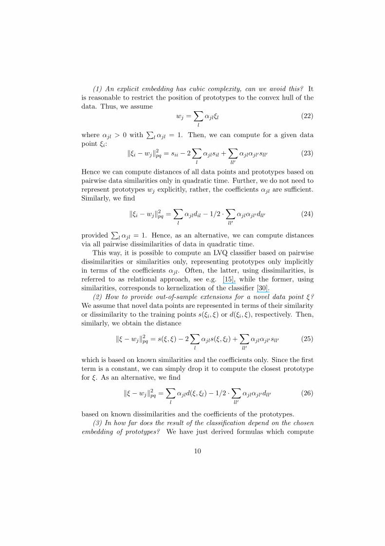
(1) An explicit embedding has cubic complexity, can we avoid this? Itis reasonable to restrict the position of prototypes to the convex hull of thedata. Thus, we assume

wj =∑

l

αjlξl (22)

where αjl > 0 with∑

l αjl = 1. Then, we can compute for a given datapoint ξi:

‖ξi − wj‖2pq = sii − 2

∑

l

αjlsil +∑

ll′

αjlαjl′sll′ (23)

Hence we can compute distances of all data points and prototypes based onpairwise data similarities only in quadratic time. Further, we do not need torepresent prototypes wj explicitly, rather, the coefficients αjl are sufficient.Similarly, we find

‖ξi − wj‖2pq =

∑

l

αjldil − 1/2 ·∑

ll′

αjlαjl′dll′ (24)

provided∑

l αjl = 1. Hence, as an alternative, we can compute distancesvia all pairwise dissimilarities of data in quadratic time.

This way, it is possible to compute an LVQ classifier based on pairwisedissimilarities or similarities only, representing prototypes only implicitlyin terms of the coefficients αjl. Often, the latter, using dissimilarities, isreferred to as relational approach, see e.g. [15], while the former, usingsimilarities, corresponds to kernelization of the classifier [30].

(2) How to provide out-of-sample extensions for a novel data point ξ?We assume that novel data points are represented in terms of their similarityor dissimilarity to the training points s(ξi, ξ) or d(ξi, ξ), respectively. Then,similarly, we obtain the distance

‖ξ − wj‖2pq = s(ξ, ξ)− 2

∑

l

αjls(ξ, ξl) +∑

ll′

αjlαjl′sll′ (25)

which is based on known similarities and the coefficients only. Since the firstterm is a constant, we can simply drop it to compute the closest prototypefor ξ. As an alternative, we find

‖ξ − wj‖2pq =

∑

l

αjld(ξ, ξl)− 1/2 ·∑

ll′

αjlαjl′dll′ (26)

based on known dissimilarities and the coefficients of the prototypes.(3) In how far does the result of the classification depend on the chosen

embedding of prototypes? We have just derived formulas which compute

10

distances in terms of the similarities/dissimilarities only. Hence the resultof the classification is entirely independent of the chosen embedding, anyother embedding which yields the same similarities/dissimilarities will givethe same result. Further, we can even ensure that the training process isindependent of the concrete embedding, provided that learning rules areexpressed in a similar way in terms of similarities or dissimilarities only.Thus, we now turn to possible training algorithms for these classifiers.

Training LVQ for (dis-)similarities

The principled way how to train such LVQ classifiers is essentially indepen-dent of the precise form of the cost function. For similarity or dissimilaritydata, there exist two different possibilities to arrive at valid training rules,concrete instances of which can be found in [30, 15]. Here, we give a morefundamental view on these two possibilities and their differences.

(1) Optimization of the cost function by computing a stochastic gradientwith respect to αjl: The cost function of both, GLVQ (2) and RSLVQ (11)has the form f(D(ξ, w)) with D(ξ, w) = (d(ξi, wj))i=1,...,N,j=1,...,m whichbecomes

f

(

sii − 2∑

l

αjlsil +∑

ll′

αjlαjl′sll′

)

i=1,...,N,j=1,...,m

(27)

for similarities or

f

(

∑

l

αjldil − 1/2 ·∑

ll′

αjlαjl′dll′

)

i=1,...,N,j=1,...,m

(28)

for dissimilarities. We can smoothly vary wj in pseudo-Euclidean spaceby adapting the coefficients αjl. The latter can be adapted by a standardgradient technique. A gradient method with respect to αjl is driven by theterm

∂f

∂αjl=∑

i

∂f((D(ξ, w))

∂d(ξi, wj)· (−2sil + 2

∑

l′

αjlsll′) (29)

if similarities are considered or by the term

∂f

∂αjl=∑

i

∂f(D(ξ, w))

∂d(ξi, wj)· (dil −

∑

l′

αjldll′) (30)

for dissimilarities, providing adaptation rules for both cost functions bymeans of a gradient descent or ascent. We can, of course, use only one

11

term corresponding to ξi in case of a stochastic gradient technique. In theserules, only pairwise similarities or dissimilarities of data are required.

As an example, the corresponding adaptation rule of RSLVQ (12) fordissimilarities, which we will refer to as relational RSLVQ in the following,yields the update rule, given a data point ξi:

∆αjl ∼

{

−(Py(j|ξi)− P (j|ξi)) · (dil −∑

l′ αjldll′) if c(wj) = yiP (j|ξi) · (dil −

∑

l′ αjldll′) if c(wj) 6= yk(31)

where the probabilities are computed as before based on the dissimilaritiesd(ξi, wj) which are expressed via dij .

Note that the parameters αjl are not yet normalized. This can beachieved in different ways, e.g. by explicit normalization after every adapta-tion step, or by the inclusion of corresponding barrier functions in the costfunction, which yields additional regularizing terms of the adaptation. Wewill use an explicit normalization in the following, i.e. after every adaptationstep, we divide the vector of coefficients by its component-wise sum.

(2) Optimization of the cost function by stochastic gradient techniqueswith respect to wj: The gradient of the cost function with respect to wj

yields∑

i

∂f((D(ξ, w))

∂d(ξi, wj)·∂d(ξi, wj)

∂wj(32)

The dissimilarity d is defined in pseudo-Euclidean space as d(ξi, wj) = (ξ −wj)

t · Ipq · (ξ − wj) where Ipq is the diagonal matrix with p entries 1 and qentries −1 as before. Thus, we obtain ∂d(ξi, wj)/∂wj = −2 · Ipq(ξi − wj).Thus, we obtain the update in a stochastic gradient method, provided onedata point ξi is chosen:

∆wj ∼ −∂f((d(ξi, wj))i,j)

∂d(ξi, wj)· Ipq

(

ξi −∑

l

αjlξl

)

(33)

The idea of the learning rule as proposed in kernel GLVQ [30] is todecompose this update into the contributions of the coefficients αjl. This ispossible iff the update rule decomposes into a sum of the form

∑

l ∆αjlξl.In this case, an update of the coefficients which is proportional to the terms∆αjl of this decomposition exactly mimics the effect of a stochastic gradientfor the prototype wj .

This decomposition, however, is usually not possible: While most com-ponents of (33) obey this form since they do not refer to components of thevector ξi, the ingredient Ipq refers to a vectorial operation which depends

12

on the pseudo-Euclidean embedding. Thus, it is in general not possible toturn this adaptation rule into a rule which can be done implicitly withoutexplicit reference to the pseudo-Euclidean embedding.

In one very relevant special case, however, it is possible: assume data areEuclidean, i.e. q = 0. In this case, we can assume without loss of generalitythat p equals the dimensionality of the vectors ξi, since components beyondp do not contribute to the distance measure in the embedding. Thus, (33)becomes

∆wj ∼∂f((d(ξi, wj))i,j)

∂d(ξi, wj)·

(

∑

l

(αjl − δil)ξl

)

(34)

with Kronecker symbol δil. Hence we obtain the update

∆αjl ∼

∂f((d(ξi,wj))i,j)∂d(ξi,wj)

· αjl if l 6= i

∂f((d(ξi,wj))i,j)∂d(ξi,wj)

· (αjl − 1) if l = i(35)

As an example, the update rule of RSLVQ (12) becomes

∆αjl ∼

−(Py(j|ξi)− P (j|ξi))αjl if l 6= i, c(wj) = yi(Py(j|ξi)− P (j|ξi))(1 − αjl) if l = i, c(wj) = yiP (j|ξi)αjl if l 6= i, c(wj) 6= yi−P (j|ξi)(1 − αjl) if l = i, c(wj) 6= yi

(36)

We refer to this update rule as kernel RSLVQ, assumed similarities are usedto compute the probabilities.

Note that this update constitutes a gradient technique only for Euclideandata. One can nevertheless apply it also for non-Euclidean settings, wherethe update step often at least improves the model since the positive partsof the pseudo-Euclidean space are usually dominant. Note that, again, nor-malization of the coefficients has to take place via direct normalization orbarrier functions, for example.

(3) How are these update rules related? The most obvious differenceof these two ways to update the coefficients consists in the fact that up-dates with respect to the coefficients follow a gradient technique whereasupdates with respect to the weights, if done implicitly without explicit ref-erence to the embedding, constitute a valid gradient method only if data areEuclidean.

But also in the Euclidean case where both updates follow a gradienttechnique, differences of the two update rules are observed. Prototypesdepend linearly on the coefficients. Hence every local optimum of the cost

13

function with respect to the weights corresponds to a local optimum withrespect to the coefficients and vice versa. As a consequence, the solutionswhich can be found by these two update rules coincide as regards the entireset of possible solutions provided the gradient techniques are designed insuch a way that local optima are reached.

However, the single update steps of the two techniques are not identical,since taking the gradient does not commute with linear operations. Thus,it is possible that different local optima are reached in a single run even ifthe methods are started from the same initial condition.

Do mathematical guarantees such as the generalization ability

transfer to the pseudo-Euclidean space?

We have already observed that one of the adaptation rules as proposed inthe literature constitutes a valid gradient technique iff data are Euclidean.There are more severe reasons why it constitutes a desired property of thedata to be Euclidean if referring to the theoretical motivation of the methodin case of RSLVQ.

RSLVQ is derived as a likelihood ratio optimization technique. Sincedistances in pseudo-Euclidean space can become negative, a Gaussian dis-tribution based on these distances does no longer constitute a valid prob-ability distribution. Thus, Euclidean data are required to preserve themathematical motivation of RSLVQ schemes as a likelihood optimizationfor (dis-)similarities.

GLVQ, in contrast, relies on the idea to optimize the hypothesis mar-gin. Generalization bounds which depend on this hypothesis margin can befound which are based on the so-called Rademacher complexity of the func-tion class induced by prototype based methods. Essentially, wide parts ofthe argumentation as given in [37] can be directly transferred to the pseudo-Euclidean setting (the situation might be more difficult if the rank of thespace is not limited and Krein spaces come into the play.) The article [37]considers the more general setting where, in addition to adaptive prototypes,the quadratic form can be learned. Here, we consider the more simple func-tion associated to GLVQ networks. Thereby, we restrict to the classificationproblems incorporating two classes 0 and 1 only, similar to [37].

In our case, the classification is based on the real-valued function

ξ 7→

(

minwi : c(wi)=0

‖wi − ξ‖2pq − minwi : c(wi)=1

‖wi − ξ‖2pq

)

(37)

the sign of which determines the output class, and the size of which de-

14

termines the hypothesis margin. This function class is equivalent to theform

ξ 7→

(

minwi : c(wi)=0

(

‖wi‖2pq − 2〈wi, ξ〉pq

)

− minwi : c(wi)=1

(

‖wi‖2pq − 2〈wi, ξ〉pq

)

)

(38)It is necessary to estimate the so-called Rademacher complexity of this func-tion class relying on techniques as introduced e.g. in [1]. Since we do notrefer to specifics of the definition of the Rademacher complexity, rather werefer to well-known structural results only, we do not introduce a precisedefinition at this place. Essentially, the complexity measures the amount ofsurprise in LVQ networks by taking the worst case correlation to randomvectors.

As in [37] a structural decomposition can take place: this function canbe decomposed into the linear combination of a composition of a Lipschitz-continuous function (min) and the function ‖wi‖

2pq − 2〈wi, ξ〉pq. We can

realize the bias ‖wi‖2pq as additional weight if we enlarge every input vector

by a constant component 1. Further, the sign of the components of wi

can be arbitrary, thus the signs in this bilinear form are not relevant andcan be simulated by appropriate weights. Thus, we need to consider alinear function in the standard Euclidean vector space. As shown in [1] itsRademacher complexity can be bounded by a term which depends on themaximum Euclidean length of ξ and wi and the square root of the numberof samples for the evaluation of Rademacher complexity. The Euclideanlengths ξ and wi can be limited in terms of the a priorly given similaritiesor dissimilarities: the vectorial representation of ξ corresponds to a columnof Q|Λ|1/2 with unitary Q and diagonal matrix of eigenvalues Λ. Thus, theEuclidean length of this vector is limited in terms of the largest eigenvalueof the similarity matrix S (or Ψ(D)). Since wi is described as a convexcombination, the same holds for wi.

As a consequence, the argumentation of [37] can be transferred imme-diately to the given setting, i.e. large margin generalization bounds holdfor GLVQ networks also in the pseudo-Euclidean setting. Since only theform of the classifier is relevant for this argumentation, but not the trainingtechnique itself, the same argumentation also holds for a classifier obtainedusing the RSLVQ cost function (11) in pseudo-Euclidean space, and it holdsfor both training schemes as introduced above.

15

How to enforce that data are Euclidean?

Albeit large margin generalization bounds transfer to the pseudo-Euclideansetting, it might be beneficial for the training prescription to transform datato obtain a purely Euclidean similarity or dissimilarity. How can data betransferred in such a way? There exist two prominent approaches, see e.g.[6, 27]:

1. clip: set all negative eigenvalues of the matrix Λ associated to thesimilarities to 0, i.e. use only the positive dimensions of the pseudo-Euclidean embedding. The corresponding matrix is referred to as Λclip.This preprocessing corresponds to the linear transformation QΛclipQ

t

of the data. The assumption underlying this transformation is thatnegative eigenvalues are caused by noise in the data, and the givenmatrix should be substituted by the nearest positive semidefinite one.

2. flip: take |Λ| instead of the matrix Λ, i.e. use the standard Euclideannorm in pseudo-Euclidean space. This corresponds to the linear trans-form Q|Λ|Qt of the similarity matrix. The motivation behind this pro-cedure is the assumption that the negative directions contain relevantinformation. Hence the simple Euclidean norm is used instead of thepseudo-Euclidean one.

Since both corrections correspond to linear transformations, their out-of-sample extension is immediate. It has already been tested in the context ofsupport vector machines (SVM) in [6] in how fare these preprocessing stepsyield reasonable results, in some cases greatly enhancing the performance.

In summary, when extending LVQ schemes to general similarities ordissimilarities, we have the choices as described in Tab. 1. These yield toeight different possible combinations. In addition, we can further preprocessdata into Euclidean form using e.g. clip or flip. Additional preprocessingsteps have been summarized in [6], for example.

As explained above, the different design decision to arrive at LVQ for(dis-)similarities differ in the following sense:

• The cost functions of RSLVQ (11) and GLVQ (2) obey different prin-ciples, relevant differences being observable already in the Euclideansetting [36]. The motivation of RSLVQ as likelihood transfers to theEuclidean setting only, while large margin bounds of GLVQ can betransferred to the pseudo-Euclidean case.

16

cost function data representation training technique

GLVQ similarity gradient w.r.t. αjl

RSLVQ dissimilarity gradient w.r.t. wj

Table 1: Different possible choices when applying LVQ schemes for (dis-)similarity data

• When turning dissimilarities into dissimilarities and backwards, theidentity is reached. When starting at similarities, however, data arecentered using this transformation.

• Training can take place as gradient w.r.t the parameters αjl or theprototypes wj. The latter constitutes a valid gradient only if dataare Euclidean, while the former follows a gradient also in the pseudo-Euclidean setting. In the Euclidean setting, the same set of localoptima is valid for both methods, but the numerical update steps canbe different resulting in different local optima in single runs.

We would like to point out that this argumentation is not restricted toLVQ schemes, rather it transfers to all prototype-based techniques providedthat the model is based on distances of the form D(ξ, w) and training takesplace by an optimization of costs of the form f(D(ξ, w)). This holds alsofor the unsupervised prototype based clustering schemes neural gas and self-organizing maps (in the form as proposed by Heskes) [23, 16] and, indeed, anextension to kernel or relational approaches is possible [29, 41, 26], wherebythe latter are often realized in form of batch updates which are particu-larly efficient for unsupervised scenarios due to closed form solutions of therespective optima [13, 5].

How to interpret prototypes for relational or kernel LVQ schemes?

One of the benefits of LVQ techniques consists in the fact that solutions arerepresented by a small number of representative prototypes which constitutemembers of the input space. In consequence, prototypes can be inspectedin the same way as data in the vectorial setting. Since the dimensionalityof points ξ is typically high, this inspection is often problem dependent:images, for example, lend itself to a direct visualization, oscillations canbe addressed via sonification, spectra can be inspected as a graph whichdisplays frequency versus intensity. Moreover, a low-dimensional projectionof the data and prototypes by means of a nonlinear dimensionality reduction

17

technique offers the possibility to inspect the overall shape of the data setand classifier independent of the application domain.

Prototypes in relational or kernel settings correspond to positions inpseudo-Euclidean space which are representative for the classes if measuredaccording to the given similarity/dissimilarity measure. Thus, prototype in-spection faces two problems: (i) the pseudo-Euclidean embedding is usuallyonly implicit, (ii) it is not clear whether dimensions in this embedding carryany semantic information. Thus, albeit prototypes are represented as linearcombinations of data also in the pseudo-Euclidean setting, it is not clearwhether these linear combinations correspond to a semantic meaning.

One approach which is taken in this context is to approximate a proto-type by one or several exemplars, i.e. members of the data set, which areclose by [17]. Thereby, the approximation can be improved if sparsity con-straints for the prototypes are integrated while training. This way, everyprototype is represented by a small number of exemplars which can be in-spected like data. Another possibility is to visualize data and prototypesusing some nonlinear dimensionality reduction technique. This enables aninvestigation of the overall shape of the classifier just as in the standardvectorial setting. Naturally, both techniques, a representation of prototypesby few exemplars as well as a projection to low dimensions incorporate er-rors depending on the dimensionality of the pseudo-Euclidean space and itsdeviation from the Euclidean norm.

4 Experiments

We test the various LVQ variants including two novel techniques which arisefrom these different combinations: relational RSLVQ trained using dissimi-larities and gradients w.r.t. αjl and kernel RSLVQ trained based on similari-ties and gradients w.r.t. wj. In the literature, the corresponding settings forGLVQ can be found [30, 15]. We compare the methods to the support vectormachine (SVM) and a k-nearest neighbor classifier (k-NN) on a variety ofbenchmarks as introduced in [6].

The data sets represent a variety of similarity matrices which are, ingeneral, non-Euclidean. It is standard to symmetrize the matrices by takingthe average of the matrix and its transposed. Further, the substitution of agiven similarity by its normalized variant constitutes a standard preprocess-ing step, arriving at diagonal entries 1. Even in symmetrized and normalizedform, the matrices do not necessarily provide a valid kernel. Hence, we alsotest the preprocessing steps clip and flip in comparison to a direct applica-

18

tion of the methods for the original data. We also report the signatures ofthe data whereby a cutoff at 0.0001 is made to account for numerical errorsof the eigenvalue solver. We also report the number of used prototypes,which is chosen as a small multiple of the number of classes. Typically,overfitting does hardly occur in LVQ settings such that the sensitivity of theresult on the number of prototypes is low, provided a sufficient flexibility ispresent.

• Amazon47 : This data set consists of 204 books written by four dif-ferent authors. The similarity is determined as the percentage of cus-tomers who purchase book j after looking at book i. This matrixis fairly sparse and mildly non-Euclidean with signature (192, 1, 11).Class labeling of a book is given by the author. The number of proto-types which is chosen in all LVQ settings is 94.

• Aural Sonar : This data set consists of 100 wide band solar signalscorresponding to two classes, observations of interest versus clutter.Similarities are determined based on human perception, averaging over5 random probands for each signal pair. The signature is (61, 38, 1).Class labeling is given by the two classes: target of interest versusclutter. The number of prototypes chosen in LVQ scenarios is 10.

• Face Rec: 945 images of faces of 139 different persons are recorded.Images are compared using the cosine-distance of integral invariantsignatures based on surface curves of the 3D faces. The signature isgiven by (45, 0, 900). The labeling corresponds to the 139 differentpersons. The number of prototypes is 139.

• Patrol : 241 samples representing persons in seven different patrol unitsare contained in this data set. Similarities are based on responses ofpersons in the units about other members of their groups. The sig-nature is (54, 66, 121). Class labeling corresponds to the seven patrolunits. The number of prototypes is 24.

• Protein: 213 proteins are compared based on evolutionary distancescomprising four different classes according to different globin families.The signature is (169, 38, 6). Labeling is given by four classes corre-sponding to globin families. The number of prototypes is 20.

• Voting : Voting contains 435 samples with categorical data comparedby means of the value difference metric. Class labeling into two classes

19

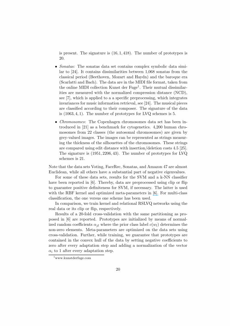
is present. The signature is (16, 1, 418). The number of prototypes is20.

• Sonatas: The sonatas data set contains complex symbolic data simi-lar to [24]. It contains dissimilarities between 1,068 sonatas from theclassical period (Beethoven, Mozart and Haydn) and the baroque era(Scarlatti and Bach). The data are in the MIDI file format, taken fromthe online MIDI collection Kunst der Fuge1. Their mutual dissimilar-ities are measured with the normalized compression distance (NCD),see [7], which is applied to a a specific preprocessing, which integratesinvariances for music information retrieval, see [24]. The musical piecesare classified according to their composer. The signature of the datais (1063, 4, 1). The number of prototypes for LVQ schemes is 5.

• Chromosomes: The Copenhagen chromosomes data set has been in-troduced in [21] as a benchmark for cytogenetics. 4,200 human chro-mosomes from 22 classes (the autosomal chromosomes) are given bygrey-valued images. The images can be represented as strings measur-ing the thickness of the silhouettes of the chromosomes. These stringsare compared using edit distance with insertion/deletion costs 4.5 [25].The signature is (1951, 2206, 43). The number of prototypes for LVQschemes is 21.

Note that the data sets Voting, FaceRec, Sonatas, and Amazon 47 are almostEuclidean, while all others have a substantial part of negative eigenvalues.

For some of these data sets, results for the SVM and a k-NN classifierhave been reported in [6]. Thereby, data are preprocessed using clip or flipto guarantee positive definiteness for SVM, if necessary. The latter is usedwith the RBF kernel and optimized meta-parameters in [6]. For multi-classclassification, the one versus one scheme has been used.

In comparison, we train kernel and relational RSLVQ networks using thereal data or its clip or flip, respectively.

Results of a 20-fold cross-validation with the same partitioning as pro-posed in [6] are reported. Prototypes are initialized by means of normal-ized random coefficients αjl where the prior class label c(wl) determines thenon-zero elements. Meta-parameters are optimized on the data sets usingcross-validation. Further, while training, we guarantee that prototypes arecontained in the convex hull of the data by setting negative coefficients tozero after every adaptation step and adding a normalization of the vectorαi to 1 after every adaptation step.

1www.kunstderfuge.com

20

k-NN SVM KGLVQ RGLVQ KRSLVQ RRSLVQ

Amayon47 28.54 (0.83) 21.46 (5.74) 22.80 (5.38) 18.17 (5.39) 15.37 (0.36) 22.44 (5.16)clip 28.78 (0.74) 21.22 (5.49) 21.95 (5.65) 23.78 (7.20) 15.37 (0.41) 25.98 (7.48)flip 28.90 (0.68) 22.07 (6.25) 23.17 (6.10) 20.85 (4.58) 16.34 (0.42) 22.80 (4.96)

Aural Sonar 14.75 (0.49) 12.25 (7.16) 13.00 (7.70) 13.50 (5.87) 11.50 (0.37) 13.00 (7.50)clip 17.00 (0.51) 12.00 (5.94) 14.50 (8.30) 13.00 (6.96) 11.25 (0.39) 13.25 (7.12)flip 17.00 (0.93) 12.25 (6.97) 12.30 (5.50) 13.00 (6.96) 11.75 (0.35) 13.50 (7.63)

Face Rec 7.46 (0.04) 3.73 (1.32) 3.35 (1.29) 3.47 (1.33) 3.78 (0.02) 7.50 (1.49)clip 7.35 (0.04) 3.84 (1.16) 3.70 (1.35) 3.81 (1.67) 3.84 (0.02) 7.08 (1.62)flip 7.78 (0.04) 3.89 (1.19) 3.63 (1.16) 3.78 (1.48) 3.60 (0.02) 7.67 (2.21)

Patrol 22.71 (0.33) 15.52 (4.02) 11.67 (4.60) 18.02 (4.65) 17.50 (0.25) 17.71 (4.24)clip 9.90 (0.16) 13.85 (4.39) 8.96 (3.90) 17.29 (3.45) 17.40 (0.29) 21.77 (7.10)flip 10.31 (0.16) 12.92 (5.09) 9.74 (4.90) 18.23 (5.10) 19.48 (0.34) 20.94 (4.51)

Protein 51.28 (0.77) 30.93 (6.79) 27.79 (7.60) 28.72 (5.24) 26.98 (0.37) 5.58 (3.49)clip 25.00 (0.74) 12.56 (5.46) 1.63 (2.10) 12.79 (5.36) 4.88 (0.17) 11.51 (5.03)flip 7.79 (0.18) 1.98 (2.85) 12.33 (6.10) 3.49 (3.42) 1.40 (0.05) 4.42 (3.77)

Voting 5.00 (0.01) 5.06 (1.84) 6.55 (1.90) 9.14 (2.10) 5.46 (0.04) 11.26 (2.23)clip 4.83 (0.02) 5.00 (1.84) 6.55 (1.90) 9.37 (2.02) 5.34 (0.04) 11.32 (2.31)flip 4.66 (0.02) 4.89 (1.78) 6.49 (1.90) 9.14 (2.22) 5.34 (0.03) 11.26 (2.43)

Sonatas 11.52 (0.20) 13.11 (2.82) 39.35 (3.17) 16.11 (3.77) 16.01 (0.11) 21.54 (4.38)clip 10.49 (0.19) 10.86 (3.74) 37.04 (4.54) 16.20 (3.73) 15.82 (0.17) 23.23 (4.41)flip 10.58 (0.25) 11.06 (3.68) 37.04 (6.41) 16.29 (3.63) 15.07 (0.12) 21.91 (4.41)

Chromosom 3.93 (0.01) 2.93 (1.07) 5.48 (0.34) 8.31 (1.84) 7.14 (0.02) 38.51 (3.61)clip 3.81 (0.01) 2.81 (1.14) 4.76 (0.00) 8.50 (1.71) 6.86 (0.02) 36.67 (3.63)flip 3.79 (0.01) 2.45 (0.98) 4.29 (0.00) 8.38 (1.76) 7.52 (0.01) 34.76 (3.20)

Table 2: Misclassification error of different dissimilarity classifiers for benchmark data as reported in [6]. Standarddeviations are given in parenthesis.

21

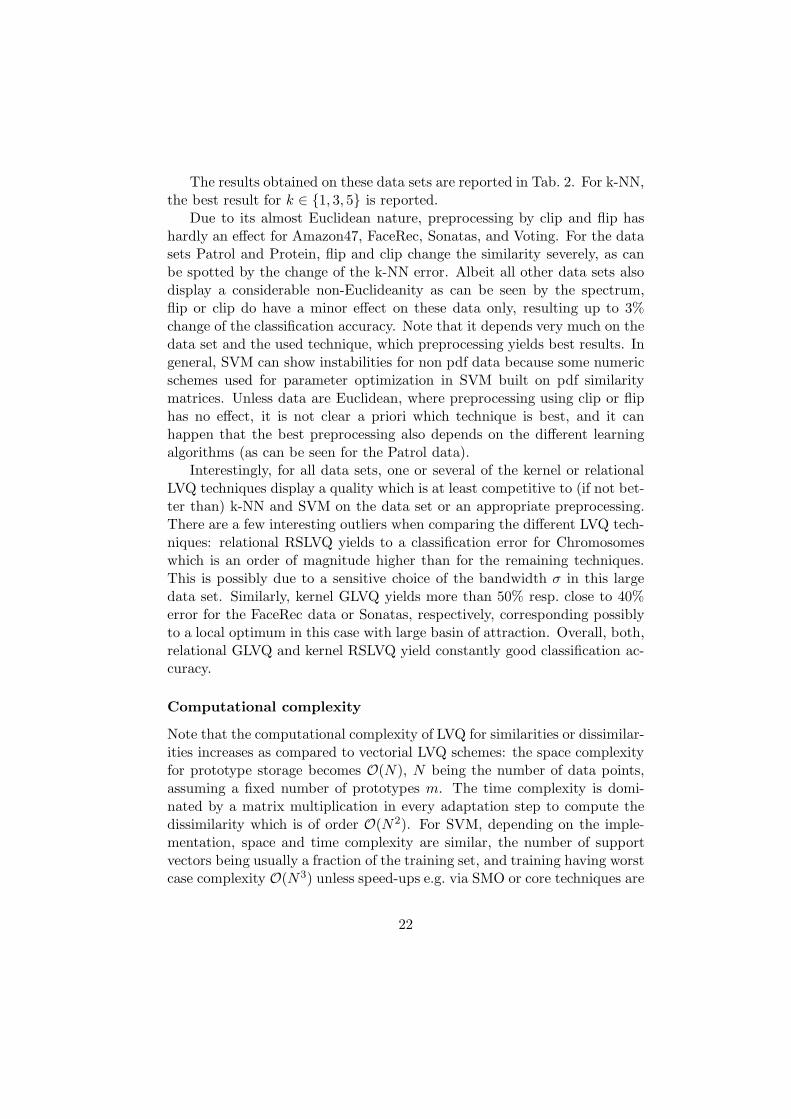
The results obtained on these data sets are reported in Tab. 2. For k-NN,the best result for k ∈ {1, 3, 5} is reported.

Due to its almost Euclidean nature, preprocessing by clip and flip hashardly an effect for Amazon47, FaceRec, Sonatas, and Voting. For the datasets Patrol and Protein, flip and clip change the similarity severely, as canbe spotted by the change of the k-NN error. Albeit all other data sets alsodisplay a considerable non-Euclideanity as can be seen by the spectrum,flip or clip do have a minor effect on these data only, resulting up to 3%change of the classification accuracy. Note that it depends very much on thedata set and the used technique, which preprocessing yields best results. Ingeneral, SVM can show instabilities for non pdf data because some numericschemes used for parameter optimization in SVM built on pdf similaritymatrices. Unless data are Euclidean, where preprocessing using clip or fliphas no effect, it is not clear a priori which technique is best, and it canhappen that the best preprocessing also depends on the different learningalgorithms (as can be seen for the Patrol data).

Interestingly, for all data sets, one or several of the kernel or relationalLVQ techniques display a quality which is at least competitive to (if not bet-ter than) k-NN and SVM on the data set or an appropriate preprocessing.There are a few interesting outliers when comparing the different LVQ tech-niques: relational RSLVQ yields to a classification error for Chromosomeswhich is an order of magnitude higher than for the remaining techniques.This is possibly due to a sensitive choice of the bandwidth σ in this largedata set. Similarly, kernel GLVQ yields more than 50% resp. close to 40%error for the FaceRec data or Sonatas, respectively, corresponding possiblyto a local optimum in this case with large basin of attraction. Overall, both,relational GLVQ and kernel RSLVQ yield constantly good classification ac-curacy.

Computational complexity

Note that the computational complexity of LVQ for similarities or dissimilar-ities increases as compared to vectorial LVQ schemes: the space complexityfor prototype storage becomes O(N), N being the number of data points,assuming a fixed number of prototypes m. The time complexity is domi-nated by a matrix multiplication in every adaptation step to compute thedissimilarity which is of order O(N2). For SVM, depending on the imple-mentation, space and time complexity are similar, the number of supportvectors being usually a fraction of the training set, and training having worstcase complexity O(N3) unless speed-ups e.g. via SMO or core techniques are

22

used.For the largest data set which we investigated (Chromosomes with 4.200

points), training one LVQ network for similarities or dissimilarities tookapproximately 15 minutes using a Matlab implementation on a powerfuldesktop computer (two six-core Xeon-processors, clocked at 3.5GHz). Withcurrent desktop computers, usually the storage of the distance matrix con-stitutes the main bottleneck concerning space (with approximately 30.000data points just fitting into current standard memory of 8 GB) - albeit thefinal classifier requires linear space only, the matrix required to representthe training data is quadratic. Such data sets would require about a daytraining time.

Thus, one the limit lies at about 30.000 data points when training theproposes LVQ techniques with current desktop computers. Similar to ap-proximation techniques for kernel methods, however, one can use approxi-mation techniques such as the Nystrom method to decrease the complexityto a linear size training set and training time, sparse approximation on theα-vectors to limit memory consumption and simplify the interpretation ofthe final prototypes, or by active learning strategies using the margin cri-terion to speed-up the learning for the online algorithms [12, 34, 35]. Thiscan extend the size of feasible data sets by one to two orders of magnitude.

5 Discussion

We have discussed different possibilities to extend LVQ classifiers to simi-larity or dissimilarity data, thereby specifying different ways how to choosethe cost function, how to include the data representation, how to train themapping, and its mutual differences. This general treatment covers severalexisting approaches in the literature and suggests a couple of new combi-nations. By relying on pseudo-Euclidean embeddings, we have developed ageneral approach how to smoothly adapt prototypes in this setting, result-ing in a well defined method for most of the techniques. Interestingly, whilegeneralization bounds can be transferred to the pseudo-Euclidean setting,a probabilistic interpretation is lost in general. Similarly, gradients withrespect to prototypes result in valid gradient techniques only in Euclideansettings, gradients with respect to coefficients can always be determined.We have evaluated the technique in a variety of benchmarks, showing sur-prisingly good classification results in several settings, albeit the underlyingtheory does not necessarily support this specific design choice as the onewith most theoretical guarantees. A more specific investigation in how far

23

non-Euclidean data are present in such situations leading e.g. to possiblynegative dissimilarities as regards prototypes will be the subject of futurework.

Acknowledgement

This work has been supported by the DFG under grants number HA2719/6-1 and HA2719/7-1 and by the CITEC center of excellence. Further, thisresearch and development project is funded by the German Federal Min-istry of Education and Research (BMBF) within the Leading-Edge ClusterCompetition and managed by the Project Management Agency Karlsruhe(PTKA). The authors are responsible for the contents of this publication.

References

[1] P. L. Bartlett, S. Mendelson. Rademacher and Gaussian Complexities:Risk Bounds and Structural Results. Journal of Machine LearningResearch, 3:463–4982, 2002.

[2] M. Biehl, A. Ghosh, and B. Hammer. Dynamics and generalization abil-ity of LVQ algorithms. Journal of Machine Learning Research, 8:323–360, 2007.

[3] M. Biehl, B. Hammer, M. Verleysen, and T. Villmann, editors. Simi-larity Based Clustering. Springer Lecture Notes Artificial IntelligenceVol. 5400/2009. Springer, 2009.

[4] C. Bishop. Pattern Recognition and Machine Learning. Springer, 2006.

[5] R. Boulet, B. Jouve, F. Rossi, and N. Villa. Batch kernel SOM andrelated Laplacian methods for social network analysis. Neurocomputing71(7-9):1257–1273. 2008.

[6] Y. Chen, E. K. Garcia, M. R. Gupta, A. Rahimi, and L. Caz-zanti. Similarity-based classification: Concepts and algorithms. JMLR,10:747–776, June 2009.

[7] R. Cilibrasi and M. B. Vitanyi. Clustering by compression. IEEETransactions on Information Theory 51(4):1523–1545, 2005.

[8] M. Cottrell, B. Hammer, A. Hasenfuss, and T. Villmann. Batch andmedian neural gas. Neural Networks, 19:762–771, 2006.

24

[9] P. Frasconi, M. Gori, and A. Sperduti. A general framework for adaptiveprocessing of data structures. IEEE TNN, 9(5):768–786, 1998.

[10] B. J. Frey and D. Dueck. Clustering by passing messages between datapoints. Science, 315:972–976, 2007.

[11] T. Gartner. Kernels for Structured Data. PhD thesis, Univ. Bonn,2005.

[12] A. Gisbrecht, B. Mokbel, F.-M. Schleif, X. Zhu, and B. Hammer. LinearTime Relational Prototype Based Learning. Int. J. Neural Syst, 22(5),2012.

[13] B. Hammer and A. Hasenfuss. Topographic mapping of large dissimi-larity datasets. Neural Computation, 22(9):2229–2284, 2010.

[14] B. Hammer, A. Micheli, and A. Sperduti. Universal approximationcapability of cascade correlation for structures. Neural Computation,17:1109–1159, 2005.

[15] B. Hammer, B. Mokbel, F.-M. Schleif, and X. Zhu. Prototype basedclassification of dissimilarity data. IDA, 2011.

[16] T. Heskes. Energy Functions for Self-Organizing Maps. In Oja, Erkki;and Kaski, Samuel (Eds.), Kohonen Maps, Elsevier, 1999.

[17] D. Hofmann and B. Hammer. Sparse approximations for kernel learningvector quantization. ESANN, 2013.

[18] P. J. Ingram, M. P. H. Stumpf, and J. Stark. Network motifs: structuredoes not determine function. BMC Genomics 7, 108, 2006.

[19] T. Kohonen. Self-Oganizing Maps. Springer, 3rd edition, 2000.

[20] T. Kohonen and P. Somervuo. How to make large self-organizing mapsfor nonvectorial data. Neural Networks 15(8-9): 945–952. 2002.

[21] C. Lundsteen, J. Phillip, and E. Granum. Quantitative analysis of 6985digitized trypsin g-banded human metaphase chromosomes. ClinicalGenetics 18(5):355–370, 1980.

[22] T. Maier, S. Klebel, U. Renner, and M. Kostrzewa. Fast and reliablemaldi-tof ms–based microorganism identification. Nature Methods, 3,2006.

25

[23] T. Martinetz, S. Berkovich, and K. Schulten. ”Neural-gas” Networkfor Vector Quantization and its Application to Time-Series Prediction.IEEE-Transactions on Neural Networks 4(4):558–569, 1993.

[24] B. Mokbel, A. Hasenfuss, and B. Hammer Graph-Based Representationof Symbolic Musical Data. GbRPR 42–51, 2009.

[25] M. Neuhaus and H. Bunke. Edit distance based kernel functions forstructural pattern classification. Pattern Recognition 39(10):1852–1863,2006.

[26] M. Olteanu, N. Villa-Vialaneix, and M. Cottrell. On-line relationalSOM for dissimilarity data. CoRR abs/1212.6316 (2012).

[27] E. Pekalska and R. P. Duin. The Dissimilarity Representation for Pat-tern Recognition. Foundations and Applications. World Scientific, 2005.

[28] O. Penner, P. Grassberger, and M. Paczuski. Sequence Alignment,Mutual Information, and Dissimilarity Measures for Constructing Phy-logenies. PLOS ONE 6(1), 2011.

[29] A. K. Qin and P. N. Suganthan. Kernel neural gas algorithms withapplication to cluster analysis. In Proc. of the 17th International Con-ference on Pattern Recognition, (ICPR ’04), 617–620, 2004.

[30] A. K. Qin and P. N. Suganthan. A novel kernel prototype-based learningalgorithm. In Proc. of the 17th International Conference on PatternRecognition (ICPR ’04), 2004.

[31] F. Rossi and N. Villa-Vialaneix. Consistency of functional learningmethods based on derivatives. Pat. Rec. Letters, 32(8):1197–1209, 2011.

[32] A. Sato and K. Yamada. Generalized Learning Vector Quantization.In NIPS 1995.

[33] F. Scarselli, M. Gori, A. C. Tsoi, M. Hagenbuchner, and G. Monfar-dini. Computational capabilities of graph neural networks. IEEE TNN,20(1):81–102, 2009.

[34] F.-M. Schleif, B. Hammer, and T. Villmann. Margin-based active learn-ing for LVQ networks. Neurocomputing 70(7-9): 1215–1224, 2007.

[35] F.-M. Schleif, T. Villmann, B. Hammer, and P. Schneider. EfficientKernelized Prototype Based Classification. Int. J. Neural Syst. 21(6):443–457, 2011.

26

[36] P. Schneider, M. Biehl, and B. Hammer. Distance learning in discrim-inative vector quantization. Neural Computation, 21:2942–2969, 2009.

[37] P. Schneider, M. Biehl, and B. Hammer. Adaptive relevance matrices inlearning vector quantization. Neural Computation, 21:3532–3561, 2009.

[38] S. Seo and K. Obermayer. Soft learning vector quantization. NeuralComput., 15:1589–1604, 2003.

[39] L. van der Maaten and G. Hinton. Visualizing high-dimensional datausing t-SNE. JMLR, 9:2579–2605, 2008.

[40] A. Vellido, J.D. Martin-Guerroro, and P. Lisboa. Making machinelearning models interpretable. In ESANN’12. 2012.

[41] Hujun Yin: On the equivalence between kernel self-organising mapsand self-organising mixture density networks. Neural Networks 19(6-7):780-784 (2006).

27