arX

iv:h

ep-t

h/94

0412

1v1

20

Apr

199

4

OPTICS, MECHANICS AND QUANTIZATION OF

REPARAMETRIZATION INVARIANT SYSTEMS †

Miguel Navarro1,2,3, Julio Guerrero2,4,and Vıctor Aldaya2,3

February 1, 2008

1.- The Blackett Laboratory, Imperial College, Prince Consort Road, LondonSW7 2BZ; United Kingdom.2.- Instituto Carlos I de Fısica Teorica y Computacional, Facultad de Ciencias,Universidad de Granada, Campus de Fuentenueva, 18002. Granada.3.- IFIC, Centro Mixto Universidad de Valencia-CSIC, Burjassot 46100-Valencia,Spain.4.- Departamento de Fısica Teorica y del Cosmos, Facultad de Ciencias, Univer-sidad de Granada, Campus de Fuentenueva, 18002. Granada.

Abstract

In this paper we regard the dynamics obtained from the Fermat principleas being the classical theory of light. We (first-)quantize the action and showhow close we can get to the Maxwell theory. We show that quantum GeometricOptics is not a theory of fields in curved space. Considering Classical Mechanicsto be on the same footing, we show the parallelism between Quantum Mechanicsand Quantum Geometric Optics. We show that, due to the reparametrizationinvariance of the classical theories, the dynamics of the quantum theories is givenby a Hamiltonian constraint. Some implications of the above analogy in thequantization of true reparametrization-invariant theories are discussed.

† Work partially supported by the D.G.I.C.Y.T.

1 Introduction.

The theory that can be properly identified with a classical theory of Optics isGeometric Optics, which is obtained from the requirement for light paths to beof extremal optical length [1]. This theory was used to describe successfully thedynamics of light until Electrodynamics were formulated and the relationshipbetween this theory and light discovered. Since then, Optics has been treatedas a chapter of Electrodynamics and its quantization has been achieved as abyproduct of Quantum Electrodynamics. Hence, the history of Optics has beenquite different from that of Mechanics, despite the close points of departure (aclassical action in both cases) and the common point of arrival (Quantum Elec-trodynamics in both cases). This paper is meant to be a small step in filling thisgap. In fact, the basics of this paper are similar to the ones that motivated theintroduction of Quantum Mechanics on the grounds of its analogy to wave optics.Nevertheless, to our knowledge, no development similar to the present one hasbeen made before.

In this paper we study firstly (Sec. 3) the theory obtained by (canonically)quantizing Geometric Optics as given by the Fermat principle†.

We shall consider two distinct interpretations of Geometric Optics: it de-scribes a particle with constant mass moving in a curved Euclidean 3+0-dimensionalspace(-time) or a particle moving in flat Euclidean 3+0-dimensional space(-time)but with a site-dependent mass. We show that, although both interpretations canbe given to the same classical dynamics, they lead to different quantum theories.In fact, quantizing the classical theory a la Proca we find that the good interpre-tation, i.e. the one that approximates Maxwell theory, is the theory of a particlewith site-dependent mass. Hence we find that, in contradiction with naıve expec-tations, Quantum Geometric Optics cannot be identified with a theory of fieldsin curved space.

The above discussion leads us naturally to discuss the case of mechanicalsystems. In Sec. 4 we discuss the optical analogy of Classical Mechanics. Weshow that a complete parallelism can be established between Geometric Opticsand “time-independent” Classical Mechanics, an analogy which can be carriedthroughout the quantization procedure, to the quantum theory. We show thatGeometric Optics and the optical “image” of Classical Mechanics are describedby reparametrization-invariant systems. Hence their quantum dynamics are tiedto a Hamiltonian constraint. As a consequence, Classical Mechanics or Geomet-ric Optics describes systems with Hamiltonian constraints whose good order isknown, as well as the physical interpretation of the associated quantum theories.In Sec. 5 we discuss some implications of these results in the quantization of true

†In some literature on the topic, the procedure that we call “quantization” is referred to as“wavization” [see for instance Ref. [2] and references therein].

1

reparametrization-invariant systems, such as gravity theories.Before pursuing the central aims of this paper we will describe briefly, in Sec.

2, the classical dynamics of (Geometric) Optics.

2 The classical dynamics of Optics.

The classical action of Optics, i.e., the action which gives the dynamics of theso-called Geometric Optics, is given by [1]:

S =∫

n(x)d s =∫

n√

x2d τ (1)

where τ parametrizes the trajectory. In this action n, the refraction index, isphysically identified with the quotient c/v where c (v) is the speed of light inthe vacuum (medium). However, unlike the mechanical case, v (n) is not adegree of freedom but a datum which must be given in advance. Since v is theonly reference to the physical time which appears in the action (1), it can besaid that the action (1) corresponds to a frozen theory, i.e., a theory withouttime. The action (1) is invariant under reparametrization: τ → τ(ξ), and thus,the study of its classical dynamics can proceed in two differents ways: a) Anon-reparametrization-invariant study which begins by fixing the parametrizationof the trajectory and b) a reparametrization-invariant, or manifestly covariant,approach which does not require such a choice.

2.1 Non-explicitly covariant approach.

Let us choose as “time”, or preferred direction of motion, the co-ordinate z. Theaction (1) takes the form

S =∫

Ld z =∫

d zn(x, y, z)√

1 + x2 + y2 (2)

The phase space is given by the co-ordinates x, y and the momenta

Px =∂L

∂x=

n2x

n√

1 + x2 + y2(3)

Py =∂L

∂y=

n2y

n√

1 + x2 + y2(4)

The Hamiltonian H takes the form

H = Pxx + Py y − L = −√

n2(x, y, z) − P 2x − P 2

y (5)

The equations of motion for any function F on the phase space are given, asusual, by

2

d F

d z= {F,H} , (6)

where the Poisson bracket is determined by the symplectic form ω, which in thecoordinates defined above has a Darboux form:

ω = d Px ∧ d x + dPy ∧ d y . (7)

2.2 Manifestly covariant description.

The action (1) has dimensions of length. In order to get an action with theadequate dimensions, it is convenient to multiply it by a factor h/λ and take

S =h

λ

∫

n(x)d s =h

λ

∫

n√

x2d τ (8)

Here h is Plank’s constant and λ should be identified with the wavelength oflight. The particular form of this factor clearly indicates that the theory we arestudying describes only light with a definite wavelength or frequency. Hence,in the present theory, photons with different wavelengths will behave as differentparticles and will not interact at all with photons with a different wavelength. Forthe same reason, the interaction with the medium, as described by the presenttheory, will preserve the wavelength of light.

The action (8) essentially admits two different interpretations, which we willrefer to in the sequel as first and second interpretations:1) It can be interpreted as a theory of a particle with site-dependent mass h

λn

evolving in a flat Euclidean 3 + 0-dimensional space(-time).2) If we introduce in (8) the refraction index into the square root we get theaction of a particle with mass h/λ moving in an euclidean 3 + 0 dimensionalspace(-time) with a conformally flat metric

d s2 = n2(dx2 + d y2 + d z2) . (9)

This analogy, together with the fact that in Electrodynamics in material mediaa tensor appears, the dielectric tensor ǫij having the form ǫij = n2δij for isotropicmedia, leads us to generalize and interpret Geometric Optics as the dynamics ofa particle with constant mass h

λmoving in a curved (Euclidean) 3+0 dimensional

space(-time).We shall study both interpretations at the same time by considering the action

of a particle with site-dependent mass hλm moving in a curved 3 + 0-dimensional

space(-time) with metric Nij . Its action is

S =h

λ

∫

md s =h

λ

∫

d τm√

Nij xixj (10)

3

The interpretation in 1) is recovered by putting m = n , Nij = δij . Theinterpretation in 2) requires m = 1 , Nij = ǫij or Nij = n2δij if the medium isisotropic.

Once the latter identifications have been made, everything proceeds as in thecase of a massive particle in a 3+1 dimensional curved space-time. The momentaare given by

pi =h

λm

Nij xj

√

Nijxixj(11)

The invariance under reparametrization of the action (10) gives rise to a con-straint:

p2 =h2

λ2m2 ⇔ N ijpipj −

h2

λ2m2 = 0 (12)

It is interesting to point out that the constraint above completely describesthe classical dynamics. In fact, following Landau [5] we can replace pi in (12) by∂S∂xi and obtain a Hamilton-Jacobi-like equation

N ij∂iS∂jS − h2

λ2m2 = 0 , (13)

for which the general solution contains all the information about the classicaldynamics of the system [4].

Obviously, equation (13) leads to the same dynamics irrespective of the inter-pretation one gives to the classical theory. In the next section we shall see thatthis is no longer the case in the quantum theory. Different interpretations of thesame classical equations lead to different quantum theories. In the present caseonly the interpretation in 1) leads to the correct quantum theory.

3 Quantization.

In this section we quantize Geometric Optics in two different ways resorting to amassive Klein-Gordon field and a Proca field, respectively [the Dirac field is notconsidered here; the interested reader can find the relevant expressions in Ref.[6]]. The two different interpretations of the classical theory discussed above lead,as we shall see, to different quantum theories. We show that only one of these canbe interpreted as the correct stationary Maxwell theory. As stated above we willdeal with both interpretations at the same time by considering the more generalcase of a particle with site-dependent mass and moving in a curved space(-time).In this and next section, indices are raised and lowered with the metric Nij .

4

3.1 Quantization as a scalar field.

As is well known, to quantize the system in (10) a la Klein-Gordon one introducesa complex scalar field φ and makes use, in eq. (12), of the basic quantizationrules: pi → −i∇i to obtain for φ the equation of motion

− h2⊔⊓φ − h2

λ2m2φ − h2αRφ = 0 (14)

or

[⊔⊓ +m2

λ2+ αR]φ = 0 . (15)

Here α is a, in principle unknown, dimensionless constant; R is the scalar curva-ture, and ⊔⊓ the Laplacian operator associated to the metric Nij ,

⊔⊓ ≡ ∇i∇i =1√N

∂i

(

N ij√

N∂j

)

, (16)

N being the determinant of the metric.The equation of motion (15) can be obtained from the action

SKG =∫

d 3x√

N

[

−N ij∂iφ∂jφ∗ +

m2

λ2φφ∗ + αRφφ∗

]

. (17)

Note that Plank’s constant has disappeared from the quantum equation ofmotion (15) for φ. Unlike the mechanical case, quantizing Geometric Opticsdoes not require the introduction of the Plank constant but another parameterλ which apparently plays a quite different role. (In the following, we shall dropthe parameter h from the “mass” h

λm).

3.2 Quantization as a Proca field.

The action of a Proca field Ai, with mass mλ, in a curved space with metric Nij

is given by [6, 7]:

SP =∫

d 3x√

N

[

−1

4F ijFij +

1

2

m2

λ2AiAi +

1

2κRAiAi +

1

2γRijA

iAj

]

(18)

whereFij = ∂iAj − ∂jAi = ∇iAj −∇jAi , (19)

and Rij , R are respectively the Ricci tensor and the scalar curvature associatedto the metric Nij. As in the scalar case, the dimensionless constants κ and γ

5

which appear in these terms are, in principle, undetermined. The equations ofmotion are easily obtained with the result

∂i

√NF ij +

√N(

m2

λ2δj

k + κRδjk + γRj

k)Ak = 0 (20)

or, what is equivalent,

∇iFij + (

m2

λ2δj

k + κRδjk + γRj

k)Ak = 0 (21)

Eq. (21) implies the following equations of motion for the basic field Ai

⊔⊓Aj −∇j(∇kAk) − Rj

kAk + (

m2

λ2δj

k + κRδjk + γRj

k)Ak = 0 . (22)

Equation (20) implies in addition

∂j(√

N(m2

λ2δj

k + κRδjk + γRj

k)Ak) = 0 ⇔ ∇j((

m2

λ2δj

k + κRδjk + γRj

k)Ak) = 0

(23)

4 Physical interpretation.

In this section we shall compare the quantum theories constructed above with theMaxwell theory. We will see that only the first interpretation of the classical the-ory gives the correct quantum one, which coincides with the stationary Maxwelltheory in a material medium. On the contrary, the interpretation of light raysas massive particles moving in a curved space does not lead to the correct wavetheory.

Maxwell equations in material media without sources read [8]:

rot E = −1

c

∂B

∂t, div B = 0 , (24)

div D = 0, rot H =1

c

∂D

∂t, (25)

which must be completed with the constitutive relations

Di =∑

j

ǫijEj , Bi =

∑

j

µijHj . (26)

In most material media the relevant constants are ǫij since µij ≈ 1. This isthe only case that we will consider in this paper.

6

The stationary equations are obtained by replacing ∂c∂t

everywhere with −iλ

,and are given by:

i

λB = rot E , rot H = − i

λD (27)

Let us consider the action

SMaxwell =∫

d 4x{−1

4FµνF

µν} , (28)

where indices are raised and lowered with the metric

d s2 =c2

n2d t2 − d r2 = v2d t2 − d r2 . (29)

With the identifications

Fµν =

0 Ex Ey Ez

−Ex 0 −Bz By

−Ey Bz 0 −Bx

−Ez −By Bz 0

, F µν =

0 −Dx −Dy −Dz

Dx 0 −Hz Hy

Dy Hz 0 −Hx

Dz −Hy Hz 0

,

(30)we get the correct Maxwell equations (24,25) (and constitutive relations (26)) inan isotropic medium with ǫ = n2 and µ = 1.

The action in (28) differs from Maxwell action in a curved space-time in thevolume element only. If we restrict the action in (28) to the stationary case,

∂2

c2∂t2≡ − 1

λ2 , and fix the gauge by putting A0 = 0, we obtain the action in (18)with a flat metric Nij = δij , and a “mass” m = n

λ. We see then that the first

interpretation of the classical theory of light, when quantized, leads to the correctquantum theory which is the stationary Maxwell theory in a material medium.

The identities in (30) imply the identifications

Di = − i

λn2Ai , (31)

Ei = − i

λAi , (32)

Bi =1

2

∑

jk

ǫijkFjk = (rot A)i , (33)

H i =1

2

∑

jk

ǫijkF jk , (34)

which give, of course, the stationary Maxwell equations in an isotropic medium(27), together with the expected constitutive relations (µ = 1),

7

D = n2E , B = H . (35)

Another proof of the equivalence above can be obtained by eliminating in (27)the magnetic field B. We are led this way to a equation of motion for E ∝ A,that coincides with eq. (22) with a flat metric and mass m = n/λ:

∇2Ei − ∂i(∂jEj) +

n2

λ2Ei = 0 . (36)

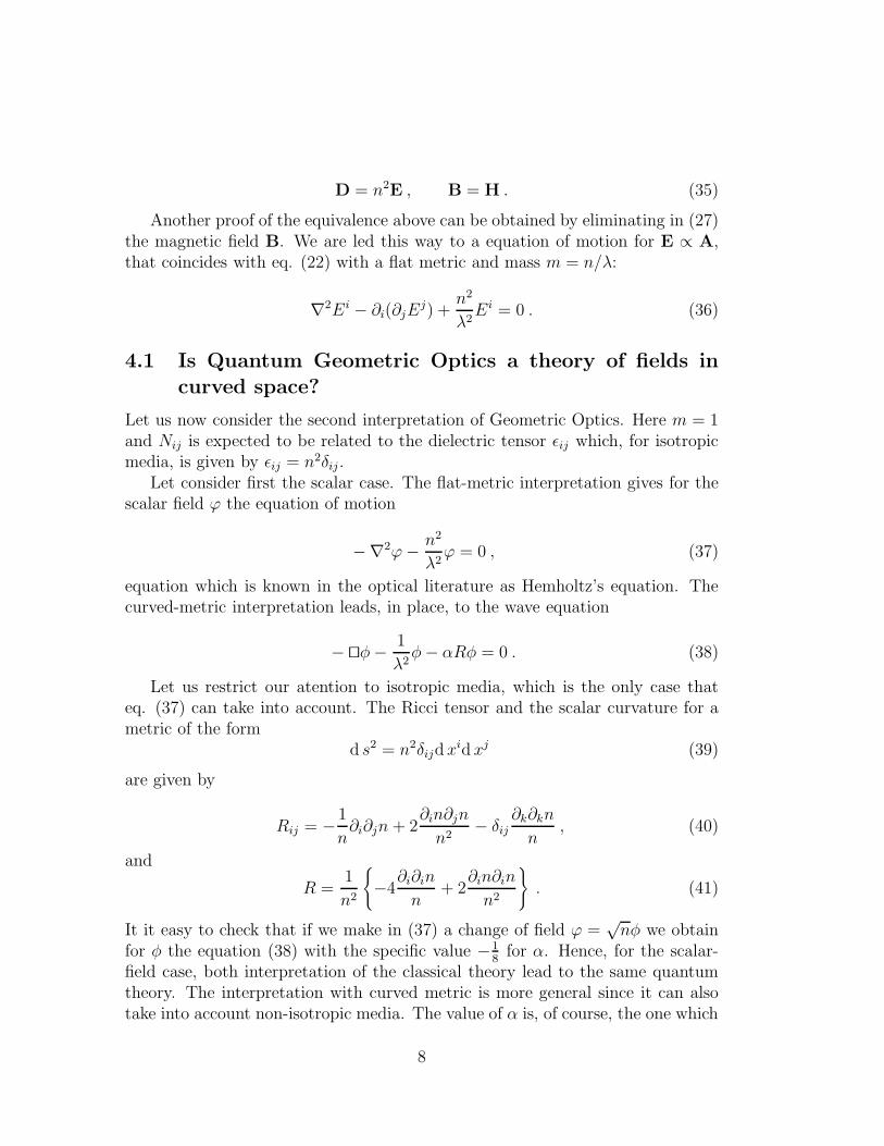
4.1 Is Quantum Geometric Optics a theory of fields in

curved space?

Let us now consider the second interpretation of Geometric Optics. Here m = 1and Nij is expected to be related to the dielectric tensor ǫij which, for isotropicmedia, is given by ǫij = n2δij .

Let consider first the scalar case. The flat-metric interpretation gives for thescalar field ϕ the equation of motion

−∇2ϕ − n2

λ2ϕ = 0 , (37)

equation which is known in the optical literature as Hemholtz’s equation. Thecurved-metric interpretation leads, in place, to the wave equation

− ⊔⊓φ − 1

λ2φ − αRφ = 0 . (38)

Let us restrict our atention to isotropic media, which is the only case thateq. (37) can take into account. The Ricci tensor and the scalar curvature for ametric of the form

d s2 = n2δijd xid xj (39)

are given by

Rij = −1

n∂i∂jn + 2

∂in∂jn

n2− δij

∂k∂kn

n, (40)

and

R =1

n2

{

−4∂i∂in

n+ 2

∂in∂in

n2

}

. (41)

It it easy to check that if we make in (37) a change of field ϕ =√

nφ we obtainfor φ the equation (38) with the specific value −1

8for α. Hence, for the scalar-

field case, both interpretation of the classical theory lead to the same quantumtheory. The interpretation with curved metric is more general since it can alsotake into account non-isotropic media. The value of α is, of course, the one which

8

corresponds, for massless scalar fields, to a conformally invariant coupling withthe metric [6]. This way of proceeding can serve as a guide to deal with the Procafield.

The flat-metric equations of motion for the Proca field are (in the followingrepeated indices are summed over except indicated otherwise):

∂iFij +n2

λ2Ai = 0 ; ∂i(n

2Ai) = 0 . (42)

In the isotropic case, the equations of motion for the curved-space Proca fieldare (Gij = ∂iCj − ∂jCi):

0 = ∂iGij −∂in

nGij +

n2

λ2Cj

+κ

{

−41

n∂i∂in + 2

∂in∂in

n2

}

Cj (43)

+γ

{

−1

n∂i∂jn + 2

∂in∂jn

n2− δij

∂k∂kn

n

}

Ci .

Let us make in (42) a change of fields Ai = nsCi. We obtain

0 = ∂iGij + s∂in

nGij +

n2

λ2Cj

+s

{

∂in

n∂iCj −

∂jn

n∂iCi

}

(44)

+s(s − 1)∂in

n

{

∂in

nCj −

∂jn

nCi

}

+ s

{

∂i∂in

nCj −

∂i∂jn

nCi

}

,

and

0 = ∂iCi + (s + 2)∂in

nCi . (45)

It is easy to check that no choice of κ, γ and s can make the wave equations (43)and (44) to coincide.

In conclusion, we can state that Quantum Geometric Optics is not a theoryof fields in curved space.

We should point out here that the conclusion above is not in contradictionwith the result obtained by Plebanski [9]. He showed that Maxwell theory in acurved space-time can be identified with the same theory in a flat space-time butevolving in a material medium. The latter identification requires, nevertheless,constitutive relations that are different from the ones we have been dealing within this paper: Di = ǫijE

j and H = B.

9

5 The optical analogy of Classical Mechanics.

As is well known [4], the trajectories with fixed energy E for a time-independentmechanical system with kinetic energy T = 1

2Mij(q)q

iqj and potential V can beobtained from the action

S = 2∫ √

E − V√

Td τ . (46)

The parameter τ has no physical relevance, since the action in (46) is reparame-trization invariant. This principle, which we shall refer to as the Maupertuisprinciple, is the mechanical analogue of the Fermat principle. Here

√E − V

plays the role of the refraction index.Let us consider a mechanical system for which Mij = mδij with m constant

(the mass of the particle). We shall see that canonical quantization of the actionin (46) gives the right time-independent Schrodinger equation.

The canonical momenta are given by

pi =

√

(E − V )√

Tmqi . (47)

The constraint associated with the reparametrization invariance of the action is

∑

i

pipi = 2m(E − V ) . (48)

If we apply the basic quantization rules pi → −ih ∂∂xi to eq. (48) we find the

stationary Schrodinger equation

− h2∇2Ψ − 2m(E − V )Ψ = 0 . (49)

We see then that the exact analogue of the time-independent Schrodingerequation for Optics is eq. (15), the Hemholtz equation, which can be written inanother way:

− λ2∇2φ − n2φ = 0 . (50)

Since n2 is always positive, the solutions of eq. (50) belong to the continuousspectrum, that is to say, they are scattering solutions and hence not normalizable.

There is a simple procedure to go from the usual Hamilton Principle to theMaupertuis Principle and vice versa. Let us start with the action in the formthat is required by the Hamilton Principle:

S =∫

d t{

1

2Mij q

iqj − (V − E)}

, (51)

10

where we have added a convenient total derivative ddt

Et to the usual Lagrangian.Let us now introduce an arbitrary parameter τ to describe the trajectories of thesystem. We have t = t(τ), d t = t′d τ (prime indicates derivative with respect tothe parameter τ). The action (51) takes the form

S =∫

d τ

{

1

2

Mijq′iq′j

t′− t′(V − E)

}

. (52)

In order to obtain a reparametrization-invariant system we now hide the relation-ship between τ and t by replacing t′ with a new quantity, the vielbein or einvein

e. We obtain

S =∫

d τ

{

1

2

Mijq′iq′j

e− e(V − E)

}

. (53)

The physical meaning of e is that of volume (length), or metric, along the tra-jectories: d t2 = e2d τ 2.

The action in (53) is, in fact, equivalent to the action that appears in theformulation of the Maupertuis principle. The quantity e plays the role of aLagrangian multiplier, and can be eliminated by using its equation of motion:

0 =δL

δe= −T

e2− (V − E) ⇒ e =

√

T

E − V(54)

If we replace in (53) e by its value in (54) we obtain the action in (46).

6 The case of true reparametrization-invariant

systems.

The procedure scketched in the previous section to obtain a reparametrization-invariant system from a mechanical one can be applied the other way round.However, the procedure when applied in this direction, is not well defined: itdoes not lead to a unique result. The reason for this ambiguity is that the samereparametrization-invariant action can be obtained from different mechanicalones. This problem can be traced back to the fact that in the reparametrization-invariant action (46) there is no way of distinguishing between kinetic and po-tential energy.

In order to ilustrate these points, let us consider, very briefly, 2-dimensionalinduced gravity which is a true reparametrization-invariant system. The action,after being restricted to the spatially homogeneous minisuperspace, reads [10]:

S =∫

d τ

[

1

2

a

eΦ′2 + 2

a′Φ′

e+

Λ

2ea

]

. (55)

11

Nevertheless, as stated above, this action is not unique: the same dynamics canbe obtained from other actions related to (55) by a redefinition of e. If we getrid of the Lagrange multiplier e we obtain

S = 2∫

d τ

√

Λ

2a

√

1

2aΦ′2 + 2a′Φ′ . (56)

The Hamiltonian constraint obtained from (55) can be written as∗

− 1

8ap2

a +1

2papΦ − Λ

2a = 0 . (57)

However, since there is no preferred choice of e here, the Hamiltonian constraintcan be written in different forms, for instance,

− 1

8(apa)

2 +1

2apapΦ − Λ

2a2 = 0 . (58)

In fact, there are physical reasons which make this latter form of the constraintpreferable [10, 11].

For Geometric Optics there are also a series of actions involving a Lagrangemultiplier (einvein) e which are equivalent to the Fermat action (1). Here, asit happens for mechanical systems, there is a prefered choice of parametrization,τ = x0, begin x0 the physical time, which obeys

x2 =1

n2. (59)

This preferred choice of parametrization singularizes, among all possible ac-tions, the one for which the interval d s2 = e2d τ 2 has the meaning of physicaltime:

d s2 ≡ d (x0)2 . (60)

This preferred action is

S =h

λ

∫

d τ

{

n2x2

e+ e

}

. (61)

However, the existence of this singularized action does not help us since it doesnot distinguish between the two interpretation of the classical theory studiedabove. In fact, it point to the wrong direction since it seems to indicate that thegood interpretation is the curved-metric one.

To summarize, we can say that the existence of a true time enables us todistinguish kinetic energy from potential energy in the classical action. This

∗Note that in the literature of Quantum Cosmology what we call quantum Hamiltonianconstraint is named Wheeler-DeWitt equation.

12

fact provides a preferred form of the classical Hamiltonian constraint which, ingeneral, makes the ordering problem of its quantum counterpart, the Schrodingerequation, less poisonous, even though the problem is not completely solved.

7 Final remarks.

The structure of the present paper have been somewhat circular: we began byconsidering Geometric Optics from the point of view of Mechanics and found theanalogy fruitful (Sections 2, 3 and 4). Then, in Sec. 5, we considered Mechanicsfrom the point of view of Geometric Optics and again found the analogy fruitful.As a result, we have studied in depth the classical and quantum dynamics ofGeometric Optics along with their relationship with Mechanics. We have widelyshown that there is a close analogy between Optics and Mechanics and thatbetween them, at a certain level, a complete isomorphism can be established.This explains the success of mechanical techniques when applied to Optics [2, 3].

The present paper ilustrates both the power and the weakness of the quantumtheory in its present form. For instance, we can obtain the stationary Maxwelltheory from the Fermat principle. However, the Fermat principle, together withthe canonical quantization procedure in its present form, does not indicate clearlywhich is the correct quantum theory. The same situation appears in connectionwith the Maupertuis principle and the time-independent Schrodinger equation.We need some information, a great amount of information indeed, that is pro-vided neither by the classical theory nor the quantization procedure. Theseexamples clearly ilustrate the difficulties which appear when quantizing truereparametrization-invariant systems such as gravity theories [12]. In fact, thequantization procedure provides neither the correct equations of the quantumtheory nor the physical interpretation we should give to it if we were able some-how to obtain these equations.

Acknowledgements. M. Navarro is grateful to the Spanish MEC for a post-doctoral FPU grant. J. Guerrero thanks the Spanish MEC for a FPU grant. M.Navarro is grateful to J. Navarro-Salas for very useful comments and suggestions.

References

[1] M. Born and E. Wolf, Principles of Optics, Pergamon, l970.

[2] T. Sekiguchi and K.B. Wolf, Am.J.Phys. 55(9)1987. K.B. Wolf, J. Math.

Phys. 33(7) 1992.

13

[3] V. Guillemin and S. Sternberg, Symplectic Techniques in Physics, CambridgeUniversity Press, 1991.

[4] H. Goldstein, Classical Mechanics 2nd edition, Addison-Wesley, Reading,Massachusetts, U.S.A.

[5] L.D. Landau and E.M. Lifshitz, The Classical Theory of Fields, PergamonPress, Oxford, 1975.

[6] N.D. Birrell and P.C.W. Davies, Quantum Fields in Curved Space, Cam-bridge University Press, 1992.

[7] L.H. Ryder, Quantum Field Theory, Cambridge University Press, 1985.

[8] L.D. Landau and E.M. Lifshitz, Electrodinamica de los Medios Continuos,Reverte, Barcelona 1975.

[9] J. Plebanski, Phys. Rev. 118, 5 (1990)1396 (See also B. Mashhoon, Phys.

Rev. D, 8, (1973)4297).

[10] J. Navarro-Salas, M. Navarro and V. Aldaya, Phys. Lett. B318 (1993).

[11] C. Teitelboim, in Quantum Theory of Gravity, ed. S. Christensen (AdamHilger, Bristol, 1984) p. 327.

[12] C.J. Isham, Conceptual and Geometrical Problems in Quantum Gravity,Imperial-TP/90-91/14.

14