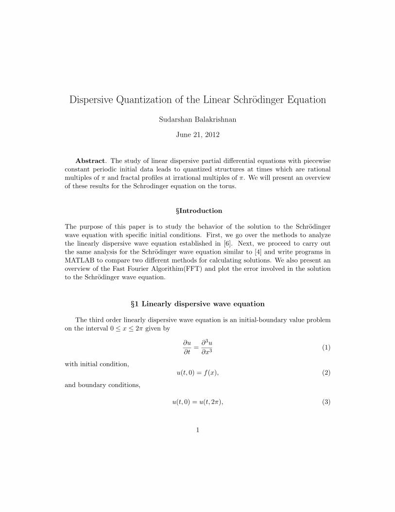
Dispersive Quantization of the Linear Schrodinger Equation

Sudarshan Balakrishnan

June 21, 2012

Abstract. The study of linear dispersive partial di↵erential equations with piecewiseconstant periodic initial data leads to quantized structures at times which are rationalmultiples of ⇡ and fractal profiles at irrational multiples of ⇡. We will present an overviewof these results for the Schrodinger equation on the torus.

§Introduction

The purpose of this paper is to study the behavior of the solution to the Schrodingerwave equation with specific initial conditions. First, we go over the methods to analyzethe linearly dispersive wave equation established in [6]. Next, we proceed to carry outthe same analysis for the Schrodinger wave equation similar to [4] and write programs inMATLAB to compare two di↵erent methods for calculating solutions. We also present anoverview of the Fast Fourier Algorithim(FFT) and plot the error involved in the solutionto the Schrodinger wave equation.

§1 Linearly dispersive wave equation

The third order linearly dispersive wave equation is an initial-boundary value problemon the interval 0 x 2⇡ given by

@u

@t=

@3u

@x3(1)

with initial condition,u(t, 0) = f(x), (2)

and boundary conditions,

u(t, 0) = u(t, 2⇡), (3)

1

@u

@x(t, 0) =

@u

@x(t, 2⇡), (4)

@2u

@x2(t, 0) =

@2u

@x2(t, 2⇡). (5)

First, we take the initial data as a unit step function

f(x) = �(x) =⇢

0 , 0 < x < ⇡;1 , ⇡ < x < 2⇡. (6)

The precise values assigned at its discontinuities are important when the problem isdiscretized, although choosing f(x) = 1

2 at x = 0, ⇡, 2⇡ is consistent with Fourier analysis.The boundary conditions allow us to extend the initial data and solution to be 2⇡ periodicfunctions in x.

In order to construct the solution, let us consider a time-dependent Fourier Series

u(t, x) ⇠1X

k=�1bk

(t)eikx. (7)

As we substitute (7) in equation (1) we get bk

(t) will satisfy the elementary linearordinary di↵erential equation:

dbk

dt= ik3b

k

(t). (8)

Then, we get:bk

(t) = bk

(0)eik

3t. (9)

Re-substituting (9) in (7), we get :

u(t, x) ⇠1X

k=�1bk

(0)ei(kx�k

3t). (10)

Observe that the solution (10) is 2⇡ periodic in both t and x. Moreover, since thek-th summand is a function of, periodic waves of frequency k move with wave speed k2ie.,!(k) = �k2, thereby justifying the dispersive nature of the system. As we solve for theinitial value problem, we note the initial condition for the Fourier series given by:

f(x) ⇠1X

k=�1ck

eikx. (11)

where we have :

ck

=12⇡

Z 2⇡

0f(x)e�ikxdx. (12)

2

Now, when we equate u(0, x) = f(x), we see that bk

(0) = ck

which will be the Fouriercoe�cients of the initial data. The step function (6), has fourier coe�cients :

bk

(0) =

8<

:

0 , k even,6= 0;i

⇡k

, k odd ;12⇡

, k= 0.(13)

Now, when we combine this with (10), we get that the solution to the linearly dispersivewave equation is given by :

u(t, x) ⇠ 12� 2

⇡

1X

j=0

sin((2j + 1)x� (2j + 1)3t)2j + 1

. (14)

§1.1 Plots

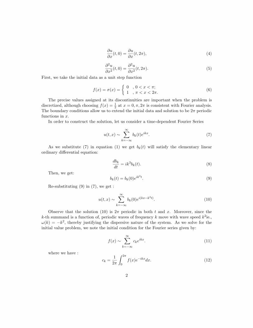
We plot the solution (14) at time t = .5⇡ and t =p

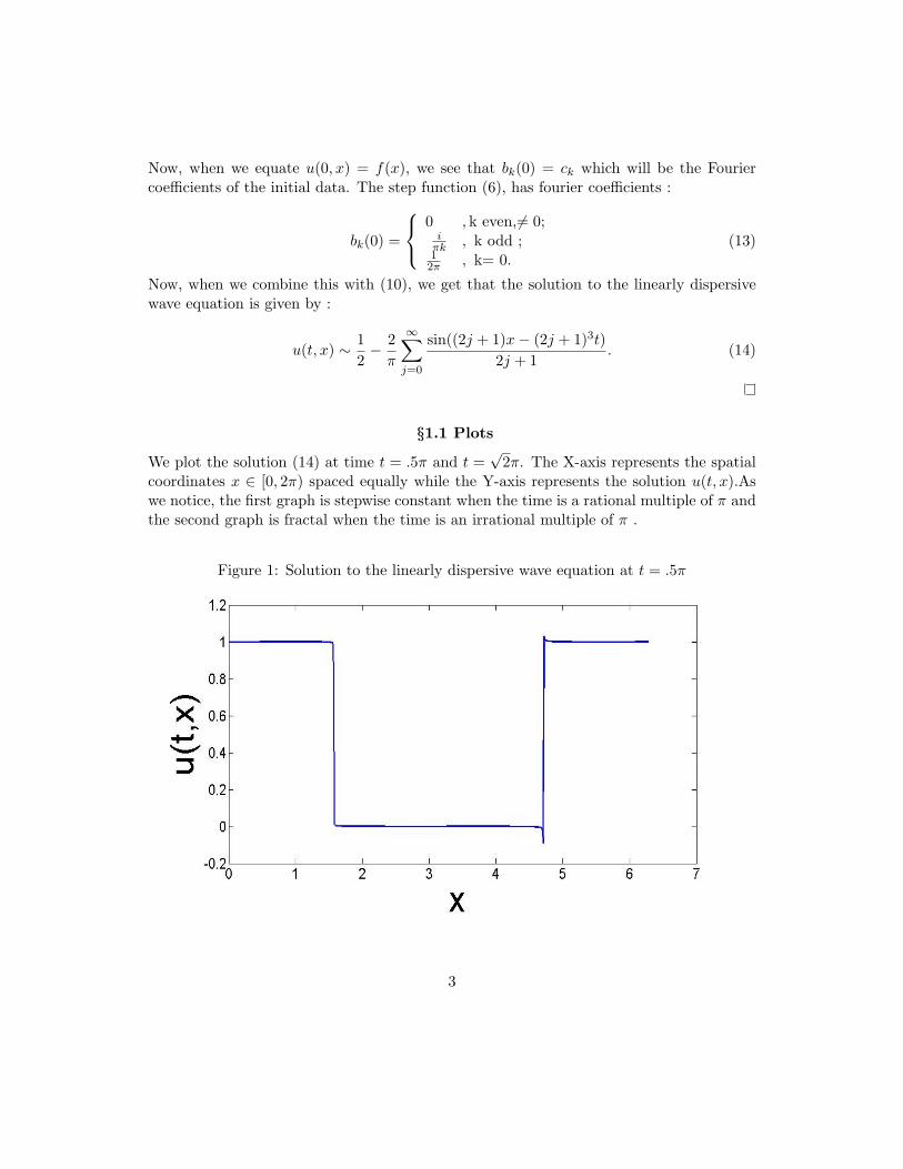
2⇡. The X-axis represents the spatialcoordinates x 2 [0, 2⇡) spaced equally while the Y-axis represents the solution u(t, x).Aswe notice, the first graph is stepwise constant when the time is a rational multiple of ⇡ andthe second graph is fractal when the time is an irrational multiple of ⇡ .

Figure 1: Solution to the linearly dispersive wave equation at t = .5⇡

3

Figure 2: Solution to the linearly dispersive wave equation at t =p

2⇡

§2. Schrodinger wave equation

The time-dependent Schrodinger equation in one dimension is:

h2

2m

@2( (x, t))@x2

+ U(x, t) (x, t) = ih@ (x, t)@t

. (15)

Here, we consider h, m both be equal to one and U(x, t) = 0. For our periodic domain0 x 2⇡ we have:

i@ (t, x)@t

=@2 (t, x)@x2

. (16)

With initial data:

(0, x) = f(x),

and boundary conditions:

(t, 0) = (t, 2⇡), (17)

x

(t, 0) = x

(t, 2⇡). (18)

We take the initial data as a unit step function:

4

f(x) = ⇣(x) =⇢�1 , 0 < x < ⇡;1 , ⇡ < x < 2⇡. (19)

Note that the boundary conditions allow us to extend the initial data and solution to be 2⇡periodic functions in x. In order to construct the solution, we have to first have to expressit as a time-dependent(complex) Fourier series:

(t, x) ⇠1X

k=�1a

k

(t)eikx (20)

where, we use ⇠ rather than = to indicate that the Fourier series is formal and, withoutadditional assumptions or analysis, its convergence is not guaranteed.As we substitute (20)in (??) to get:

eikx

da

k

dt

�=

⇥ik2a

k

(t)⇤eikx (21)

After equating the coe�cients of the individual exponentials on both sides, we noticethat a

k

(t) satisfies an elementary linear ordinary di↵erential equation:

dak

dt= ik2a

k

(t), (22)

Now, solving (22) using the separation of variables we get:

ak

(t) = ak

(0)eik

2t, (23)

and after substituting (23) in (20), the solution is:

(t, x) =1X

k=�1a

k

(0)eik

2t+ikx (24)

Observe that the solution (24) is 2⇡ periodic in both t and x. We note the Fourier seriesexpansion of the initial condition is given by:

f(x) =1X

k=�1bk

eikx (25)

In order to compute the coe�cients of this Fourier series, we note that in {eikx} is anorthonormal basis for the initial data.We will use this property in our computation[2], fork, l 2 N we have:

Z 2⇡

0eikxe�ilxdx =

⇢2⇡ , k = l;0 , k 6= l. (26)

5

Multiplying (25) by e�ilx on both sides, we notice:

f(x)e�ilx =

( 1X

k=�1bk

eikx

)e�ilx (27)

Integrating both sides from 0 to 2⇡ we get:

Z 2⇡

0f(x)e�ilxdx =

Z 2⇡

0{1X

k=�1bk

eikx}e�ilxdx. (28)

Z 2⇡

0f(x)e�ilxdx =

Z 2⇡

0bl

eikx�ilxdx. (29)

bk

=12⇡

Z 2⇡

0f(x)e�ikxdx. (30)

Equating (0, x) = f(x), we notice that ak

(0) = bk

are the Fourier coe�cients of the giveninitial data. Evaluating this integral:

bk

=12⇡

Z 2⇡

0f(x)e�ikxdx =

12⇡

Z⇡

0e�ikxdx (31)

bk

=12⇡

e�ikx

�ik

���⇡

0(32)

In order to integrate the expression e�ciently, we use Euler’s identity

ei⇡ = �1 (33)

eki⇡ =⇢�1 k odd ;+1 k even.

(34)

Our integral evaluates to:

bk

= ak

(0) =⇢ �

1⇡ik

�k odd ;

0 k even.(35)

Note, here that when k=0, we have that ak

(0) equals zero. Now, when we combine thiswith (24), we get the solution to the Schrodinger equation is given by :

(t, x) =1⇡i

1X

k=�1

ei((2k+1)2t+(2k+1)x)

2k + 1(36)

6

§2.1 Plots

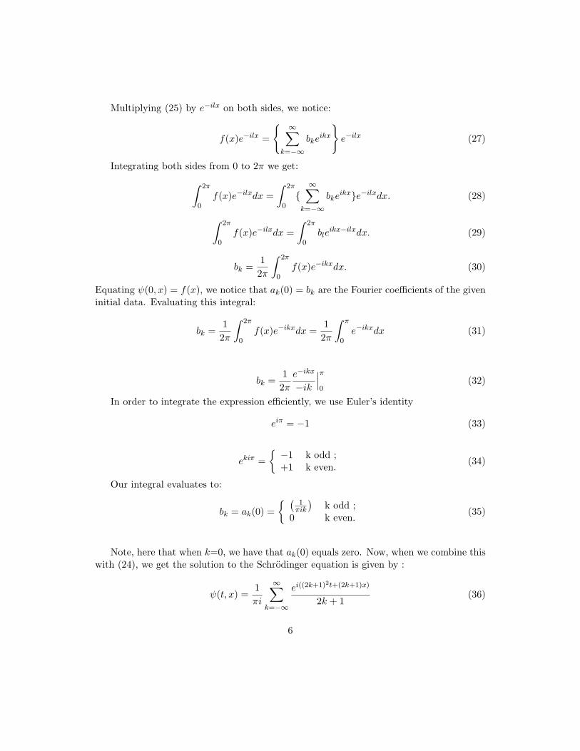
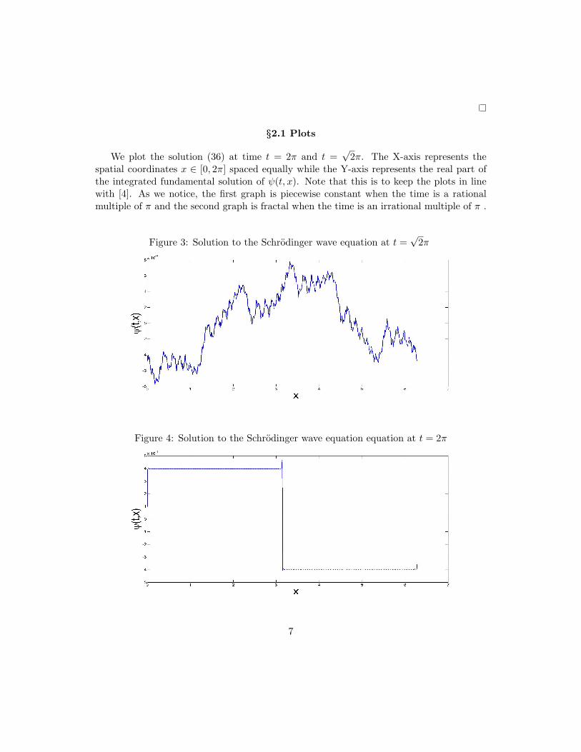
We plot the solution (36) at time t = 2⇡ and t =p

2⇡. The X-axis represents thespatial coordinates x 2 [0, 2⇡] spaced equally while the Y-axis represents the real part ofthe integrated fundamental solution of (t, x). Note that this is to keep the plots in linewith [4]. As we notice, the first graph is piecewise constant when the time is a rationalmultiple of ⇡ and the second graph is fractal when the time is an irrational multiple of ⇡ .

Figure 3: Solution to the Schrodinger wave equation at t =p

2⇡

Figure 4: Solution to the Schrodinger wave equation equation at t = 2⇡

7

§3 Quantization on a periodic domain

Similar to [6] and [4], the following theorem establishes the behavior of the solution tothe Schrodinger equation at subintervals of rational multiples of ⇡

Let

p

q

2 Q be a rational number. Then the solution (t, x) = 1⇡i

P1j=�1

e

i((2j+1)2t+(2j+1)x)

2j+1

to the Schrodinger equation at time t = p⇡

q

is constant on every subinterval

⇡j

q

< x < ⇡(j+1)q

for j = 0, ..., 2q � 1.

Proof

A function h(x) which satisfies the above theorem is a linear combination

h(x) =2q�1X

j=0

aj

�j,q(x). (37)

Where �j,q(x) represents the compressed box functions:

�j,q(x) =

(1, ⇡j

q

< x < ⇡(j+1)q

, 0 j 2q � 1.

0, otherwise.(38)

The box function (37) has Fourier coe�cients:

cj,q

k

=12⇡

Z 2⇡

0�j,q(x)e�ikxdx =

12⇡

Z ⇡(j+1)q

⇡j

q

e�ikxdx =12⇡

e�ikx

�ik

���⇡(j+1)

q

⇡j

q

(39)

=

(i(e�i⇡k/q�1)e�i⇡jk/q

2⇡k

, k 6= 0,12q

, k = 0.(40)

The Fourier coe�cients of (37) are a linear combination of the individual Fourier coef-ficients (40)

ck

=2q�1X

j=0

aj

cj,q

k

. (41)

Note that, k takes values {�q . . . q � 1} and given c�q

. . . cq�1 and (27) corresponds

to the indices k = {�q . . . q � 1}. This forms a system of 2q linear equations for the 2qunknown coe�cients a0, ..., a2q�1.

ck

=2q�1X

j=0

aj

cj,q

k

. (42)

8

Let ck

denote the rescaled Fourier coe�cients. Observe that they satisfy:

ck

=12q

2q�1X

j=0

aj

e�i⇡jk/q. (43)

First, when k = 0, we have that

ck

=12q

2q�1X

j=0

aj

e�i⇡jk/q =12q

2q�1X

j=0

aj

=2q�1X

j=0

12q

aj

= c0. (44)

Next, when 0 6= k ⌘ 0 mod 2q, observe that from (39) cj,q

k

= 0 and consequently by(41) c

k

= 0. This implies that the rescaled coe�cients are also correspondingly zero.Now, when k 6⌘ 0 mod 2q by (41) and (40)(mere rearrangement of terms), we have

that:

ck

=⇡kc

k

iq(e�i⇡k/q � 1)(45)

In e↵ect, we have:

ck

=

8><

>:

ck

= 0, 0 6= k ⌘ 0 mod 2q,⇡k

iq(e�i⇡k/q)�1ck

, k 6⌘ 0 mod 2q,ck

= c0, k = 0(46)

Now, we know that {ei⇡jl/q} is orthonormal and it satisfies:

2q�1X

j=0

ei⇡jl/qe�i⇡j

0l/q =

⇢2q, j = j

0 0 j 2q � 1.

0, j 6= j0,

(47)

Multiplying both sides by ei⇡j

0l/q in (43)

cl

ei⇡j

0/q =

0

@ 12q

2q�1X

j=0

aj

e�i⇡jl/q

1

A ei⇡j

0l/q (48)

Taking the sum from l = �q to l = q � 1 in (48), we get:

q�1X

l=�q

cl

ei⇡j

0/q =

q�1X

l=�q

0

@ 12q

2q�1X

j=0

aj

e�i⇡jl/q

1

A ei⇡j

0l/q (49)

By (47), we have that only the j0-th summand remains:

9

q�1X

l=�q

cl

ei⇡j

0/q =

q�1X

l=�q

12q

(aj

0 ) (50)

q�1X

l=�q

cl

ei⇡j

0/q = a

j

0 (51)

Therefore, 2q rescaled coe�cients ˆc�q

, ..., ˆcq�1 will satisfy the discrete Fourier Transform

of a0, ..., a2q�1 [3] and by reconstruction we have that:

aj

=q�1X

l=�q

cl

ei⇡ljk/q, j = 0, ..., 2q � 1. (52)

Hence, by (40), the rescaled Fourier coe�cients (46) will satisfy

ck

= cl

, k ⌘ l 6⌘ 0mod2q (53)

and

ck

= 0, 0 6= k ⌘ l ⌘ 0mod2q (54)

This shows us that the function that is constant on every subinterval ⇡j

q

< x < ⇡(j+1)q

if the Fourier coe�cients satisfy (46). The Fourier coe�cients of the solution (36) at thetime t = ⇡p

q

are:

ck

= ak

✓⇡p

q

◆= a

k

(0)eik

2 ⇡p

q (55)

If k ⌘ l mod 2q, then k3 ⌘ l3 mod 2q and

eik

2⇡

p

q = eil

2⇡

p

q (56)

Notice that (56) implies that the rescaled Fourier coe�cients (46) will be piecewiseconstant. This proves the theorem.

§4 Quantization with Delta functions

The Fourier coe�cients of a function f(x) are q-periodic in their indices, so ck+q

= ck

for all k, if and only if the series represents a linear combination of q(periodically extended)

10

delta functions concentrated at the nodes which are rational multiples of ⇡, xj

= 2⇡j/q for

j = 0, 1, ..., q � 1:

f(x) =q�1X

j=0

aj

�(x� 2⇡j/q)

Proof

First, we have that the series represents a linear combination of q delta functions con-centrated at the rational nodes x

j

= 2⇡j/q for j = 0, 1, ..., q � 1. Now, to justify theintegrability of the delta function, let us construct our delta function as follows:

�(x) = lim✏!0

12✏

e�x

2

✏ . (57)

Now, for points xj

= 2⇡j/q :

�(x� 2⇡j/q) = lim✏!0

12✏

e�(x�2⇡j/q)2

✏ . (58)

Constructing the Fourier coe�cients similar to §3 we have that,

cj,q

k

=12⇡

Z 2⇡

0�(x� 2⇡j/q)e�ikxdx. (59)

We will simplify (59), using the following lemma:

§4.1 Lemma

For a given Dirac delta function �(x) and a continuous function f(x) at x0:

f(x0) =Z +1

�1�(x� x0)f(x)dx. (60)

Proof

First, consider an ✏ interval of x0, for this interval notice that f(x0) is approximatelyconstant. So, we have:

Zx0+✏

x0�✏

�(x�x0)f(x)dx =Z

x0+✏

x0�✏

�(x�x0)f(x0)dx = f(x0)Z

x0+✏

x0�✏

�(x�x0) = f(x0). (61)

Note thatR

x0+✏

x0�✏

�(x�x0) = 1, follows from the definition of the delta function. In (59),we have that:

11

cj,q

k

=12⇡

Z 2⇡

0�(x� 2⇡j/q)e�ikxdx = e�ik(2⇡j/q). (62)

Now, let us compute cj,q

k+q

:

cj,q

k+q

= e�ik+q(2⇡j/q) = e�ik(2⇡j/q)+q(2⇡j) = e�ik(2⇡j/q) = cj,q

k

(63)

Note, that the last relation in (63) is true by Euler’s Identity.The Fourier coe�cients are a linear combination of (63) ie:

ck

=q�1X

j=0

aj

cj,q

k

(64)

Since,cj,q

k+q

= cj,q

k

, we have that:

ck

=q�1X

j=0

aj

cj,q

k

=q�1X

j=0

aj

cj,q

k+q

= ck+q

(65)

§5 Quantization with the fundamental solution

As we saw in the previous section, the periodicity with respect to the Fourier coe�cientsimplies the delta functions are concentrated at certain rational nodes. We observe the samewith the fundamental solution to the Schrodinger wave equation.

Suppose t = ⇡p/q is a rational multiple of ⇡. Then the fundamental solution to the

Schrodinger wave equation is a linear combination of periodically extended delta functions.

When p is odd, the 2q delta functions are concentrated at the rational nodes xj

= ⇡j/q for

j = 0, ..., 2q � 1, whereas for p even, the q delta functions are concentrated at xj

= 2⇡j/qfor j = 0, ..., q � 1.

Proof

We know that the fundamental solution to the initial boundary value problem on a periodicdomain is given by:

F (t, x) ⇠ 12⇡i

1X

k=�1

(�1)k

kei(kx+k

2t). (66)

As we have studied previously, we know that the solution is given by a complex Fourierseries:

12

F (t, x) ⇠1X

k=�1bk

(t)eikx. (67)

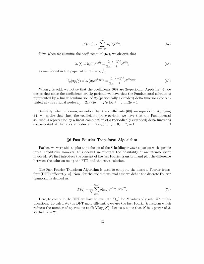
Now, when we examine the coe�cients of (67), we observe that

bk

(t) = bk

(0)eik

2t =

12⇡i

(�1)k

keik

2t, (68)

as mentioned in the paper at time t = ⇡p/q:

bk

(⇡p/q) = bk

(0)eik

2⇡p/q =

12⇡i

(�1)k

keik

2⇡p/q. (69)

When p is odd, we notice that the coe�cients (69) are 2q-periodic. Applying §4, wenotice that since the coe�cients are 2q periodic we have that the Fundamental solution isrepresented by a linear combination of 2q-(periodically extended) delta functions concen-trated at the rational nodes x

j

= 2⇡j/2q = ⇡j/q for j = 0, ..., 2q � 1

Similarly, when p is even, we notice that the coe�cients (69) are q-periodic. Applying§4, we notice that since the coe�cients are q-periodic we have that the Fundamentalsolution is represented by a linear combination of q-(periodically extended) delta functionsconcentrated at the rational nodes x

j

= 2⇡j/q for j = 0, ..., 2q � 1

§6 Fast Fourier Transform Algorithm

Earlier, we were able to plot the solution of the Schrodinger wave equation with specificinitial conditions, however, this doesn’t incorporate the possibility of an intrinsic errorinvolved. We first introduce the concept of the fast Fourier transform and plot the di↵erencebetween the solution using the FFT and the exact solution.

The Fast Fourier Transform Algorithm is used to compute the discrete Fourier trans-form(DFT) e�ciently [5]. Now, for the one dimensional case we define the discrete Fouriertransform is defined as:

F (y) =1N

N�1X

x=0

�(xn

)e�2⇡ix

n

y

n

/N . (70)

Here, to compute the DFT we have to evaluate F (y) for N values of y with N2 multi-plications. To calculate the DFT more e�ciently, we use the fast Fourier transform whichreduces the number of operations to O(N log2 N). Let us assume that N is a power of 2,so that N = 2n.

13

We define !N

to be the N th root of unity given by !N

= e2⇡i/N and with L = N

2 andwe have:

F (y) =1

2L

2L�1X

x=0

f(x)!xy

2L

. (71)

Splitting (70), we get:

F (y) =12

1L

L�1X

x=0

f(2x)!(2x)y2L

+1L

L�1X

x=0

f(2x + 1)!(2x+1)y2L

!. (72)

In (72), since the square of a 2Lth root of unity is also an Lth root of unity, we havethat !

(2x)y2L

= !xy

L

and thereby:

F (y) =12

1L

L�1X

x=0

f(2x)!xy

L

+1L

L�1X

x=0

f(2x + 1)!xy

L

!y

2L

!. (73)

Now, we can represent F (y) by:

F (y) =12�F

e

(y) + Fo

(y)!y

2L

�, (74)

where Fe

(y) and Fo

(y) represent the former and latter sums in (73). Both, Fe

(y) andF

o

(y) are discrete Fourier transforms over L = N

2 points.Now, with

!L+y

L

= !y

L

!L+y

2L

= �!y

2L

, (75)

we have that:

F (y + L) =12�F

e

(y)� Fo

(y)!y

2L

�. (76)

Now,we can compute the discrete Fourier transform with N -points by dividing F (y) fory = 0, ..., L�1 for the first sum and the second sum can be computed for y = M, ..., 2M�1.

Now, let g(n) denote the time take to perform compute a transform of size N = 2n,measured by the number of multiplications and additions carried out. From the above, wenotice that:

g(n) = 2g(n� 1) + 2n�1. (77)

In order to compute the inverse discrete Fourier transform, we first have that:

F (y) =1N

N�1X

x=0

f(x)e�2⇡ixy/N . (78)

14

It’s inverse is given by,

f(x) =N�1X

x=0

F (y)e2⇡ixy/N . (79)

Taking the complex conjugate of (79), we get:

ˆf(x) =N�1X

x=0

ˆF (y)e�2⇡ixy/N . (80)

As we notice (80) looks like the Discrete fourier transform, the same algorithm toapplied to the Discrete fourier transform can now be applied.

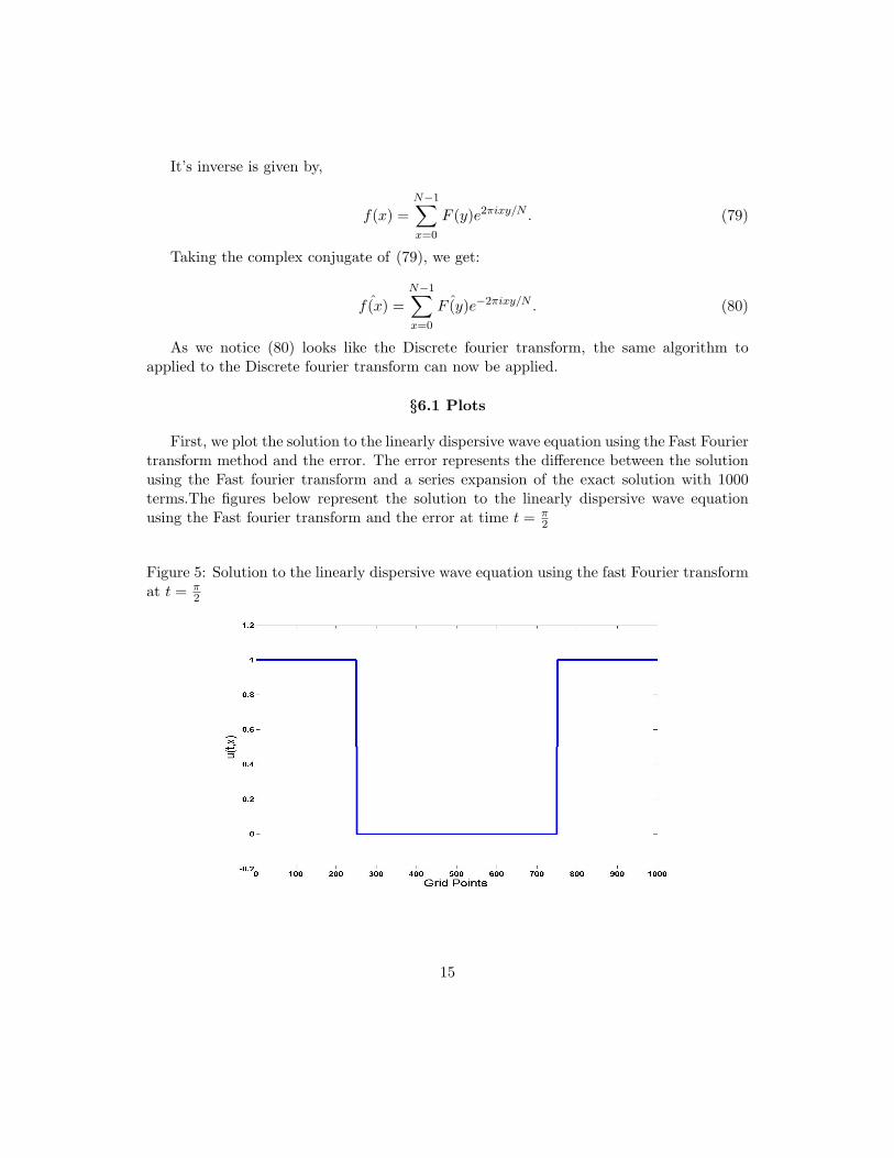
§6.1 Plots

First, we plot the solution to the linearly dispersive wave equation using the Fast Fouriertransform method and the error. The error represents the di↵erence between the solutionusing the Fast fourier transform and a series expansion of the exact solution with 1000terms.The figures below represent the solution to the linearly dispersive wave equationusing the Fast fourier transform and the error at time t = ⇡

2

Figure 5: Solution to the linearly dispersive wave equation using the fast Fourier transformat t = ⇡

2

15

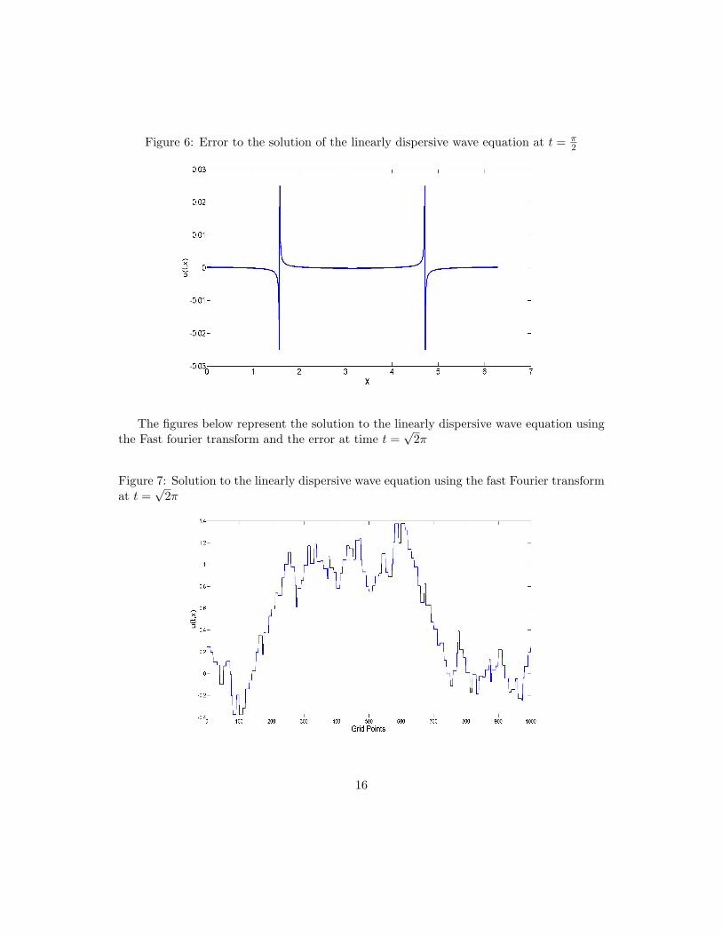
Figure 6: Error to the solution of the linearly dispersive wave equation at t = ⇡

2

The figures below represent the solution to the linearly dispersive wave equation usingthe Fast fourier transform and the error at time t =

p2⇡

Figure 7: Solution to the linearly dispersive wave equation using the fast Fourier transformat t =

p2⇡

16

Figure 8: Error to the solution of the linearly dispersive wave equation at t =p

2⇡

As we observe there is a visible di↵erence between both solutions. It is at presentunclear which expression is more accurate. We leave this as the subject of future research.

§Conclusion

This paper establishes a foundation for further work on extending the properties of Schrodingerwave equation. This can be any of the following:1. To study the invariance properties of dispersive wave equations that lead to novel reci-procity relations and other identities for the associated number-theoretic Weyl exponentialsums.2.The Talbot e↵ect has been experimentally observed in both optics and atoms. Can onedesign experiments that exhibit such behavior in other dispersive media? [1]

§Acknowledgements

First, I would like to thank Benson Muite for his patient and meticulous advice. I amalso deeply indebted to the Undergraduate Research Opportunity Program(UROP) andthe Research Experience for Undergraduates(REU) for their generous funding. I wouldalso like to thank Gong Chen for his help as well as Brandon Cloutier and Paul Rigge fortheir feedback. Finally, I’d like to thank the Brian Hall, Arlo Cain, Will Kirwin and PeterMiller from the Notre Dame summer school for quantization for their help.

17

References

[1] M.V Berry. Quantum carpets, carpets of light. Physics World, 60:39–44, 2001.

[2] R. Bracewell. The Fourier Transform and Its applications. Prentice Hall, 1992.

[3] J.O Smith III. Mathematics of the Discrete Fourier Transform. W3K Publishing, 2007.

[4] Oskolov K.I. Schrodinger equation and oscillatory Hilbert transforms of second degree.Fourier Anal. Appl, 4:341–356, 1998.

[5] Dave Marshall. Fast Fourier Transform, 1997.

[6] P.J. Olver. Dispersive quantization. Amer. Math. Monthly, 117:599–610, 2010.

§Appendix

MATLAB program to plot the linearly dispersive wave equation

% This function plots the solution to the linearlydispersive wave equation. First, save the file in asuitable folder and change the matlab environment to thatparticular folder. One can call the function by giving asuitable value for the time and position, note here thatthe position is an array of numbers.function [result] = qd(t,x) %Name of the function.dmn = size(x);%Size of the position array.x_d = dmn(2);result = zeros(size(x));%Providing the size of result.sum_t = zeros(size(x));%Providing the size of sum_t%For loop to recursively compute the solution.%For loop to recursively compute the solution.for i = 1:x_d

for j = 0:x_dsum_t(i) = sum_t(i) + (sin(((2*j+1)*x(i))-((2*j+1)^3)*t)/(2*j+1));

endtend%For loop to compute the final solution.for k = 1:x_d

result(k) = .5 - (2/pi)*sum_t(k);

18

endplot(x,result); % Plot the solutionxlabel(’x ’,’FontSize’,14); % Labeling the x axisylabel(’u(t,x)’,’FontSize’,14); % Labeling the y axistitle(’Solution to the linearly dispersive waveequation’,’FontSize’,14);% Providing the title to thegraph.

MATLAB program to plot the Schrodinger wave equation

%This function plots the solution to the Schr\{o}dingerwave equation. First, save the file in a suitable folderand change the matlab environment to that particularfolder. One can call the function by giving a suitablevalue for the time and position, note here that theposition is an array of numbers.function [ result ] = schrqd( t,x )%Name of the function.

dmn = size(x);%Size of the position array.x_d = dmn(2);result = zeros(size(x));%Providing the size of result.sum_t = zeros(size(x));%Providing the size of sum_t%For loop to recursively compute the solution.for i = 1:x_dfor j = 0:1000

sum_t(i) = sum_t(i) + (sin(((2*j+1)*x(i))+((2*j+1)^2)*t)/(2*j+1));endend%For loop to compute the final solution.for k = 1:x_dresult(k) = (2/(pi*i))*sum_t(k);end

plot(x,real(result)); % Plot the real part of solutionxlabel(’x ’,’FontSize’,14); % Labeling the x axisylabel(’u(t,x)’,’FontSize’,14); % Labeling the y axistitle(’Solution to the Schrodinger wave equation at t = 2\pi’,’FontSize’,14); ;% Providing the title to the graph.

19

end

MATLAB program to plot the solution using the fast Fourier transform

%This program computes the solution to the linearly dispersivewave equation using the fast fourier transform.N = 1000; %Number of grid points.h = 2*pi/N; %Defining the size of each grid.x = h*(1:N); %Defining the variable x as an array.t = .05*pi; %Defining the variable t as a rational multiple of \pi.dt = .001; % Defining an appropriate time step.u0 = zeros(1,N); %Defining the initial datau0(N/2+1:N)= ones(1,N/2); % Defining the initial datak=(1i*[0:N/2-1 0 -N/2+1:-1]);k3=k.^3;u=ifft(exp(k3*t).*fft(u0));%Solution to the Linearly dispersive wave equation.plot(u)%Command to plot the solution

MATLAB program to plot errror to the solution to the linearly dispersive

wave equation

%This program computes the error to the solution to thelinearly dispersive wave equationN = 1000; %Number of stepsh = 2*pi/N; %step sizex = h*(1:N);t = sqrt(2)*pi;u0(1) = .0; % Setting the initial values for the discontinuitiesu0(2:N/2 -1) = 0;u0(N/2) = 0.5;u0(N/2 +1:N-1) = 1;u0(N)=0.5;k=(i*[0:N/2-1 0 -N/2+1:-1]);k3=k.^3;u=ifft(exp(k3*t).*fft(u0));plot(x, qd(t,x)-u);xlabel(’x ’,’FontSize’,14);ylabel(’u(t,x)’,’FontSize’,14);title(’Error at time .5 *\pi’,’FontSize’,14);

20