VQQL. Applying Vector Quantization toReinforcement Learning

Fernando Fernandez and Daniel Borrajo

Universidad Carlos III de MadridAvda. de la Universidad, 30

28912 Leganes. Madrid (Spain)ffernand@scalab.uc3m.es, dborrajo@ia.uc3m.es

http://scalab.uc3m.es/∼ffernand, http://scalab.uc3m.es/∼dborrajo

Abstract Reinforcement learning has proven to be a set of success-ful techniques for finding optimal policies on uncertain and/or dynamicdomains, such as the RoboCup. One of the problems on using such tech-niques appears with large state and action spaces, as it is the case ofinput information coming from the Robosoccer simulator. In this paper,we describe a new mechanism for solving the states generalization prob-lem in reinforcement learning algorithms. This clustering mechanism isbased on the vector quantization technique for signal analog-to-digitalconversion and compression, and on the Generalized Lloyd Algorithmfor the design of vector quantizers. Furthermore, we present the VQQLmodel, that integrates Q-Learning as reinforcement learning techniqueand vector quantization as state generalization technique. We show someresults on applying this model to learning the interception task skill forRobosoccer agents.

1 Introduction

Real world for autonomous robots is dynamic and unpredictable. Thus, for mostrobotic tasks, having a perfect domain theory (model) of how the actions ofthe robot affect the environment is usually an ideal. There are two ways ofproviding such models to robotic controllers: by careful and painstaking “ad-hoc” manual design of skills; or by automatically acquiring such skills. Therehave been already many different approaches for learning skills in robotic tasks,such as genetic algorithms [6], or neural networks and EBL [13].

Among them, reinforcement learning techniques have proven to be veryuseful when modeling the robot worlds as MDP or POMDP problems [1, 12,17]. However, when using reinforcement learning techniques with large stateand/or action spaces, two efficiency problems appear: the size of the state-actiontables and the correct use of the experience. Current solutions to this problemrely on applying generalization techniques to the states and/or actions. Somesystems have used decision trees [3], neural networks [9], or variable resolutiondynamic programming [14].

1

In this paper, we present an approach to solve the generalization problemthat uses a numerical clustering method: the generalized Lloyd algorithm forthe design of vector quantizers [10]. This technique is extensively employed forsignal analog-to-digital conversion and compression, which have common char-acteristics to MDP problems. We have used Q-Learning [18] as reinforcementlearning algorithm, integrating it with vector quantization techniques in theVQQL model.

We have applied this model for compacting the set of states that a Robosoc-cer agent perceives, thus dramatically reducing the reinforcement table size. Inparticular, we have used the combination of vector quantization and reinforce-ment learning for acquiring the ball interception skill for agents playing in theRobosoccer simulator [16].

We introduce the reinforcement learning and the Q-learning algorithm insection 2. Then, the vector quantization technique and the generalized Lloydalgorithm are described in section 3. Section 4 describes how vector quantizationis used to solve the generalization problem in the model VQQL, and in sections 5and 6, the experiments performed to verify the utility of the model and the resultsare shown. Finally, the related work and conclusions are discussed.

2 Reinforcement Learning

The main objective of reinforcement learning is to automatically acquire knowl-edge to better decide what action an agent should perform at any moment tooptimally achieve a goal. Among many different reinforcement learning tech-niques, Q-learning has been very widely used [18]. The Q-learning algorithm fornon deterministic Markov decision processes is described in table 1 (executionof the same action from the same state by an agent arrives to different states, sodifferent rewards could be obtained). It needs a definition of the possible states,S, the actions that the agent can perform in the environment,A, and the rewardsthat it receives at any moment for the states it arrives to after applying eachaction, r. It dynamically generates a reinforcement table Q(s, a) (using equa-tion 1) that allows it to follow a potentially optimal policy. Parameter γ controlsthe relative importance of future actions rewards with respect to immediate re-wards. Parameter α refers to the probabilities involved, and it is computed usingequation 2.

Qn(s, a)← (1− αn)Qn−1(s, a) + αn{r + γ maxa′

Qn−1(s′, a′)} (1)

αn ← 1

1 + visitsn(s, a)(2)

where visitsn(s, a) is the total number of times that the state-action entryhas been visited.

2

Q-learning algorithm (S,A)For each pair (s ∈ S, a ∈ A), initialize the table entry Q(s, a) to 0.Observe the current state sDo forever– Select an action a and execute it– Receive immediate reward r– Observe the new state s′

– Update the table entry for Q(s, a) using equation 1– Set s to s′

Table1. Q-learning algorithm.

3 Vector Quantization (VQ)

Vector quantization appeared as an appropriate way of reducing the number ofbits needed to represent and transmit information [7]. In the case of large statespaces in reinforcement learning, the problem is analogous: how can we compactlyrepresent a huge number of states with very few information? In order to applyvector quantization to the reinforcement learning problem, we will provide firstsome definitions.

3.1 Definitions

Since our goal is to reduce the size of the reinforcement table, we have to find outa more compact representation of the states.1 If we have K attributes describingthe states, and each attribute ai can have values(ai) different values, where thisnumber is usually big (in most cases infinite, since they are represented with realnumbers), then the number of potential states can be computed as:

S =K∏

i=1

values(ai) (3)

Since this can be a huge number, the goal is to reduce it to N � S new states.These N states have to be able to approximately capture the same informationas the S states; that is, all similar states in the previous representation, belongto the same new state in the new representation. The first definition takes thisinto account.

Definition 1. A vector quantizer Q of dimension K and size N is a mappingfrom a vector (or a “point”) in the K-dimensional Euclidean space, RK , intoa finite set C containing N output or reproduction points, called code vectors,codewords, or codebook. Thus,

Q : RK −→ C

where C = (y1, y2, . . . , yN), yi ∈ RK .

1 We will refer indistinctly to vectors and states.

3

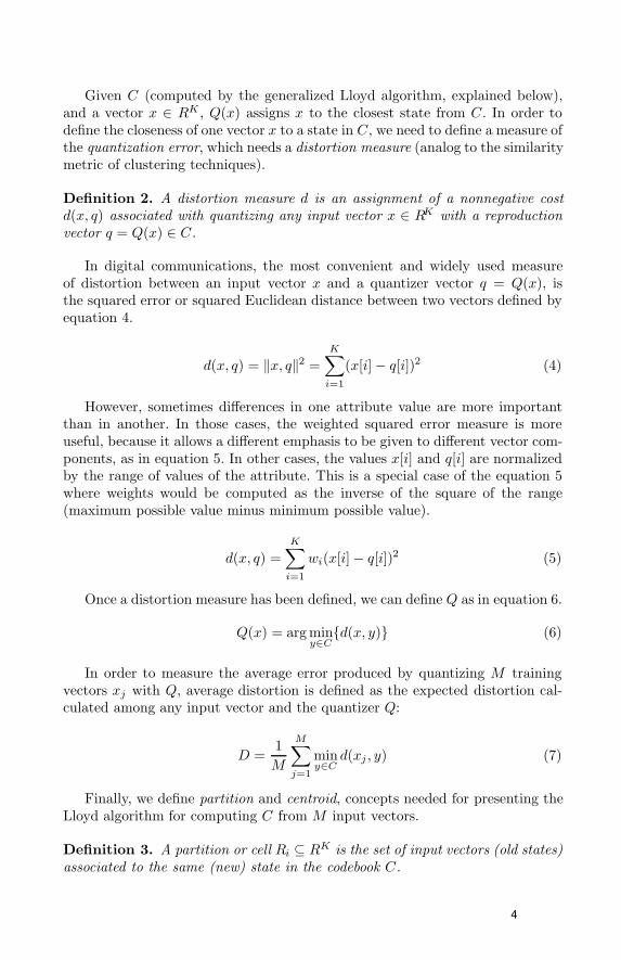
Given C (computed by the generalized Lloyd algorithm, explained below),and a vector x ∈ RK , Q(x) assigns x to the closest state from C. In order todefine the closeness of one vector x to a state in C, we need to define a measure ofthe quantization error, which needs a distortion measure (analog to the similaritymetric of clustering techniques).

Definition 2. A distortion measure d is an assignment of a nonnegative costd(x, q) associated with quantizing any input vector x ∈ RK with a reproductionvector q = Q(x) ∈ C.

In digital communications, the most convenient and widely used measureof distortion between an input vector x and a quantizer vector q = Q(x), isthe squared error or squared Euclidean distance between two vectors defined byequation 4.

d(x, q) = ‖x, q‖2 =K∑

i=1

(x[i]− q[i])2 (4)

However, sometimes differences in one attribute value are more importantthan in another. In those cases, the weighted squared error measure is moreuseful, because it allows a different emphasis to be given to different vector com-ponents, as in equation 5. In other cases, the values x[i] and q[i] are normalizedby the range of values of the attribute. This is a special case of the equation 5where weights would be computed as the inverse of the square of the range(maximum possible value minus minimum possible value).

d(x, q) =K∑

i=1

wi(x[i]− q[i])2 (5)

Once a distortion measure has been defined, we can define Q as in equation 6.

Q(x) = arg miny∈C{d(x, y)} (6)

In order to measure the average error produced by quantizing M trainingvectors xj with Q, average distortion is defined as the expected distortion cal-culated among any input vector and the quantizer Q:

D =1

M

M∑

j=1

miny∈C

d(xj , y) (7)

Finally, we define partition and centroid, concepts needed for presenting theLloyd algorithm for computing C from M input vectors.

Definition 3. A partition or cell Ri ⊆ RK is the set of input vectors (old states)associated to the same (new) state in the codebook C.

4

Definition 4. We define the centroid, cent(R), of any set R ⊆ RK as thatvector y ∈ RK that minimizes the distortion between any point x in R and y:

cent(R) = {y ∈ RK | E[d(x, y)] ≤ E[d(x, y′)], ∀x ∈ R, y′ ∈ RK} (8)

where E[z] is the expected value of z.

A common formula to calculate each component i of the centroid of a parti-tion is given by equation 9.

cent(R)[i] =1

‖R‖‖R‖∑

j=1

xj [i] (9)

where xj ∈ R, xj [i] is the value of component (attribute) i of vector xj , and‖R‖ is the cardinality of R.

3.2 Generalized Lloyd Algorithm (GLA)

The generalized Lloyd algorithm is a clustering technique, extension of the scalarcase [11]. It consists of a number of iterations, each one recomputing the set ofmore appropriate partitions of the input states (vectors), and their centroids.The algorithm is shown in table 2. It takes as input a set T of M input states,and generates as output the set C of N new states (quantization levels).

Generalized Lloyd algorithm (T,N)1. Begin with an initial codebook C1.2. Repeat

(a) Given a codebook (set of clusters defined by their centroids) Cm ={yi; i = 1, . . . , N}, redistribute each vector (state) x ∈ T into one ofthe clusters in Cm by selecting the one whose centroid is closer to x.

(b) Recompute the centroids for each cluster just created, using the cen-troid definition in equation 9 to obtain the new codebook Cm+1.

(c) If an empty cell (cluster) was generated in the previous step, an alter-native code vector assignment is made (instead of the centroid com-putation).

(d) Compute the average distortion for Cm+1, Dm+1

Until the distortion has only changed by a small enough amount since lastiteration.

Table2. The generalized Lloyd algorithm.

There are three design decisions to be made when using such technique:

Stopping criterion Usually, average distortion of codebook at cycle m, Dm,is computed and compared to a threshold θ (0 ≤ θ ≤ 1) as in equation 10.

5

(Dm −Dm+1)/Dm < θ (10)

Empty cells One of the most used mechanisms consists of splitting other par-titions, and reassigning the new partition to the empty one. All empty cellsgenerated by the GLA are changed in each iteration by another cell. To de-fine the new one, another non-empty cell with big average distortion y, issplitted in two:

y1 = {y[1]− ε, . . . , y[K]− ε}, and

y2 = {y[1] + ε, . . . , y[K] + ε}Initial codebook generation We have used a version of the GLA as explained

in table 3, that requires a partition split mechanism as the one describedabove inserted into the GLA in table 2.

GLA with Splitting (T )1. Begin with an initial codebook C1 with N (number of levels of the code-

book) set to 1. The only level of the codebook is the centroid of the input.2. Repeat

(a) Set N to N ∗ 2(b) Generate a new codebook Cm+1 with N levels that includes the code-

book Cm. The rest N undefined levels can be initialized to 0(c) Execute the GLA algorithm in table 2 with the splitting mechanism

with parameters (T,N) over the codebook obtained in previous stepUntil N is the desired level

Table3. A version of the generalized Lloyd algorithm that solves the initial codebookand empty cell problems.

4 Application of VQ to Q-learning. VQQL

The use of vector quantization and the generalized Lloyd algorithm to solvethe generalization problem in reinforcement learning algorithms requires twoconsecutive phases:

Learn the quantizer. Or to design the N -levels vector quantizer from inputdata obtained from the environment.

Learn the Q function. Once the vector quantizer is designed (we have clus-tered the environment in N different states), it is needed to learn the Qfunction, generating the Q table, that will be composed of N rows, and acolumn for each action (one could also use the same algorithm for quantizingactions).

We have two ways of unifying both phases:

6

Off-line mode. We could obtain the information required to learn the quan-tizer and the Q function, and, later, learn both.

On-line mode. We could obtain data to generate only the vector quantizer,and, later, the Q function is learned by the interaction of the agent with theenvironment, using the previously designed quantizer.

The advantages of the first one are that it allows to use the same informationseveral times, and the quantizer and the Q table are learned with the same data.The second one allows the agent to use greedy strategies in order to increase thelearning rate (exploration versus exploitation).

In both cases, the behavior of the agent, once the quantizer and the Q func-tion are learned, is the same; a loop that:

– Receives the current state, s, from the environment.– Obtains the quantization level, s′, or state to which the current state belongs.– Obtains the action, a, from the Q table with bigger Q value for s′.– Executes action a.

5 The Robosoccer domain

In order to verify the usefulness of the vector quantization technique to solve thegeneralization problem in reinforcement learning algorithms, we have selected arobotic soccer domain that presents us all the problems that we have defined inprevious sections. The RoboCup, and its Soccer Server Simulator, gives us theneeded support [16].

The Soccer Server provides an environment to confront two teams of players(agents). Each agent perceives at any moment two types of information: visualand auditorial [16]. Visual information describes a player what it sees in the field.For example, an agent sees other agents, field marks such as the center of thefield or the goals, and the ball. Auditorial information describes a player what ithears in the field. A player can hear messages from the referee, from its coach, orfrom other players. Any agent (player) can execute actions such as run (dash),turn (turn), send messages (say), kick the ball (kick), catch the ball (catch), etc.

One of the more basic skills a soccer player must have is ball interception. Theimportance of this skill comes from the dependency that other basic skills, suchas kick or catch the ball, have with this one. Furthermore, ball interception ispresented as one of the more difficult tasks to solve in the Robosoccer simulator,and it has been studied in depth by other authors [17]. In the case of Stone’swork, neural networks were used to solve the ball interception problem posed asa supervised learning task.

The essential difficulties of this skill come from the visual limitations of theagent, as well as from the noise that the simulator includes in movements ofobjects. In order to intercept the ball, our agents parse the visual informationthat they receive from the simulator, and obtain the following information:2

2 The Robosoccer simulator protocol version 4.21 has been used for training. In otherversions of the simulator, other information could be obtained.

7

– Relative Distance from the ball to the player.– Relative Direction from the ball to the player.– Distance Change, gives an idea of how Distance is changing.– Direction Change, gives an idea of how Direction is changing.

In order to intercept the ball, after knowing the values of these parameters,each player can execute several actions:

Turn changing the direction of the player according to a moment between -180and 180 degrees.

Dash increasing the velocity of the player in the direction it is facing with apower between -30 and 100.

To reduce the number of possible actions that an agent can perform (gener-alization over actions problem), we have used macro-actions defined as follows.Macro-actions are composed of two consecutive actions: turn(T ), and dash(D),resulting in turn-dash(T,D). We have selected D = 100, and T is computedaccording to A+∆A, where A is the angle between the agent and the ball, and∆A can be: +45,+10,0,-10,-45. Therefore, we have reduced the set of actions tofive actions.

6 Results

In this section, the results of using the VQQL model for learning the ball inter-ception skill in the Robosoccer domain are shown. In order to test the perfor-mance of the Lloyd algorithm, we generated a training set of 94.852 states withthe following iterative process, similar to the one used in [17]:

– The goalie starts at a distance of four meters in front of the center of thegoal, facing directly away from the goal.

– The ball and the shooter are placed randomly at a distance between 15 and25 from the defender.

– For each training example, the shooter kicks the ball towards the center ofthe goal with a maximum power (100), and an angle in the range (−20, 20).

– The defender goal is to catch the ball. It waits until the ball is at a distanceless or equal than 14, and starts to execute actions defined in section 5,while the goal is not in the catchable area [16]. Currently, we are only givingpositive rewards. Therefore, if the ball is in the catchable area, the goalietries to catch the ball, and if it succeeds, a positive reward is given to thelast decision. If the goalie does not catch the ball, it can execute new actions.Finally, if the shooter goals, or the ball goes out of the field, it receives areward of 0.

Then, we used the algorithm described in Section 3 with different numberof quantization levels (new states). Figure 1 shows the evolution of the aver-age distortion of the training sequence. The x-axis shows the logarithm of the

8

number of quantization levels, i.e. the number of different states what will beused afterwards by the reinforcement learning algorithm and the y-axis showsthe average distortion obtained by GLA. The distortion measure used has beenthe quadratic error, as shown in equation 4. As it can be seen, when using 26 to28 quantization levels, the distortion becomes practically 0.

0

200

400

600

800

1000

1200

0 2 4 6 8 10 12 14

Dis

tort

ion

log2 N

Distortion Evolution

Figure1. Average distortion evolution depending on the number of states in the code-book.

To solve the state generalization problem, a single mechanism could be used,such as a typical scalar quantization on each parameter. In this case, the averagequantization error, following the error quadratic distortion measure defined inequation 4, could be calculated as follows. The Distance parameter range isusually in (0.9,17.3). Thus, if we allow 0.5 as the maximum quantization error,we need around 17 levels. Direction is in the (-179,179) range, so, if we allow aquantization error of 2, 90 levels will be needed. Distance Change parameter isusually in (-1.9,1), so we need close to 15 levels, allowing an error of 0.1, andDirection Change is usually in (-170,170), so we need 85 levels, allowing an errorof 2. Then, following equation 3 we need 17∗90∗15∗85 = 1, 950, 750 states!!! Thisis a huge size for a reinforcement learning approach. Also, the average distortionthat is obtained according to equation 4 is:

(0.5

2)2 + (

2

2)2 + (

0.1

2)2 + (

2

2)2 = 2.7

given that the quantization error on each quantization is half of the maximumpossible error. Instead, using the generalized Lloyd algorithm, with many lessstates, 2048, the average distortion goes under 2.0. So, it reduces both the numberof states to be represented, and the average quantization error.

Why is this reduction possible on the quantization error? The answer is givenby the statistical advantages that the vector quantization provides over the scalarquantization. These advantages can be seen in Figure 2. In Figure 2(a), onlythe pairs of Distance and Direction that appeared in the training vectors havebeen plotted. As we can see, only some regions of the bidimensional space havevalues, showing that not all combinations of the possible values of the Distanceand Direction parameters exist in the training set of input states. Therefore, the

9

reinforcement tables do not have to consider all possible combinations of thesetwo parameters. Precisely, this is what vector quantization does. Figure 2(b)shows the points considered by 1024 states quantization. As it can be seen, itonly generates states that represent minimally the states in the training set. Thefact that there are parts of the space that are not covered by the quantizationis due to the importance of the other two factors not considered in the figure(change in distance and direction).

-200

-150

-100

-50

0

50

100

150

200

0 2 4 6 8 10 12 14 16 18 20

Dire

ctio

n

Distance

Parameters (Distance Direction)

-200

-150

-100

-50

0

50

100

150

200

0 2 4 6 8 10 12 14 16 18

Dire

ctio

n

Distance

Parametres (Distance Direction)

(a) (b)

Figure2. Distance and Direction parameters from (a) original data, and (b) a codebookobtained by the GLA.

In order to test what the best number of quantization levels is, we havevaried that number, and learned a Q table per obtained quantizer. We measuredsuccessful performance as the percentage of kicks of a new set of 100 testingproblems that go towards the goal, and are catched by the goalie. The resultsof these experiments are shown in Figure 3. In that figure the performance ofthe goalie is shown, depending of the size of the Q table. As a reference, arandom goalie would only achieve a 20% of success, and a goalie with the mostused heuristic of always go towards the ball achieves only a 25% of successfulbehavior. As it can be seen, Q table sizes less than 128 obtain a quasi-randombehavior. From sizes of the Q table from 128 to 1024, the performance increasesuntil the maximum performance obtained, which is close to 60%. From 4096states and up, the performance decreases. That might be the effect of obtainingagain a very large domain (huge number of state).

7 Related Work

Other models to solve the generalization problem in reinforcement learning usedecision trees as in the G-learning algorithm [3], and kd-trees (similar to a deci-sion tree) in the VRDP algorithm [14]. Another solution is Moore’s PartiGamealgorithm [15] or neural networks [9]. One advantage of vector quantization isthat it allows to easily define control parameters for obtaining different behaviorsof the reinforcement learning technique. The main two parameters that have tobe defined are number of quantization levels, and average distortion (similarity

10

0.25

0.3

0.35

0.4

0.45

0.5

0.55

0.6

0.65

4 5 6 7 8 9 10 11 12 13go

als(

%)

log2 N

Learning Performance

Figure3. Learning performance depending on the number of states in the codebook.

metric). Other approaches to this problem were proposed in [5] and [2] wherebayesian networks are used. Similar ideas to our approach to Vector Quantiza-tion have been used by other researchers, as in [4] where Q-Learning is used asin this paper, using LVQ [8]. Again, it is easier for VQ to define its learningparameters than it is for neural networks based systems.

8 Conclusions and Future Work

In this paper, we have shown that the use of vector quantization for the gen-eralization problem of reinforcement learning techniques provides a solution tohow to partition a continuous environment into regions of states that can beconsidered the same for the purposes of learning and generating actions. It alsosolves the problem of knowing what granularity or placement of partitions ismore appropriate.

However, this mechanism introduces a set of open questions that we expectto tackle next. As we explained above, the GL algorithm allows us to generatecodebooks or sets of states of different sizes, each of them giving us differentquantization errors. So, an important question is the relation between the num-ber of quantization levels and the performance of the reinforcement learningalgorithm. Another important issue relates to whether this technique can beapplied not only to the state generalization problem, but also to actions gen-eralization. We are also currently exploring the influence of providing negativerewards to the reinforcement learning technique. Finally, in the short term weintend to compare it against using decision trees and LVQ.

References

1. Jacky Baltes and Yuming Lin. Path-tracking control of non-holonomic car-likerobot with reinforcement learning. In Manuela Veloso, editor, Working notes ofthe IJCAI’99 Third International Workshop on Robocup, pages 17–21, Stockholm,Sweden, July-August 1999. IJCAI Press.

11

2. Craig Boutilier, Richard Dearden, and Moises Goldszmidt. Exploiting structurein policy construction. In Proceedings of the Fourteenth International Joint Con-ference on Artificial Intelligence (IJCAI-95), pages 1104–1111, Montreal, Quebec,Canada, August 1995. Morgan Kaufmann.

3. David Chapman and Leslie P. Kaelbling. Input generalization in delayed rein-forcement learning: An algorithm and performance comparisons. Proceedings ofthe International Joint Conference on Artificial Intelligence, 1991.

4. C. Claussen, S. Gutta, and H. Wechsler. Reinforcement learning using funtionalapproximation for generalization and their application to cart centering and frac-tal compression. In Thomas Dean, editor, Proceedings of Sixteenth InternationalJoint Coference on Artificial Intelligence, volume 2, pages 1362–1367, Stockholm,Sweden, August 1999.

5. Thomas Dean and Robert Givan. Model minimization in markov decision pro-cesses. In Proceedings of the American Association of Artificial Intelligence (AAAI-97). AAAI Press, 1997.

6. Marco Dorigo. Message-based bucket brigade: An algorithm for the appointment ofcredit problem. In Yves Kodratoff, editor, Machine Learning. European Workshopon Machine Learning, LNAI 482, pages 235–244. Springer-Verlag, 1991.

7. Allen Gersho and Robert M. Gray. Vector Quantization and Signal Compression.Kluwer Academic Publishers, 1992.

8. T. Kohonen. The self-organizing map. In Proceedings of IEEE, volume 2, pages1464–1480, 1990.

9. Long-Ji Lin. Scaling-up reinforcement learning for robot control. In Proceedings ofthe Tenth International Conference on Machine Learning, pages 182–189, Amherst,MA, June 1993. Morgan Kaufman.

10. Yoseph Linde, Andre Buzo, and Robet M. Gray. An algorithm for vector quantizerdesign. In IEEE Transactions on Communications, Vol1. Com-28, No 1, pages 84–95, 1980.

11. S. P. Lloyd. Least squares quantization in pcm. In IEEE Transactions on Infor-mation Theory, number 28 in IT, pages 127–135, March 1982.

12. S. Mahavedan and J. Connell. Automatic programming of behavior-based robotsusing reinforcement learning. Artificial Intelligence, 55:311–365, 1992.

13. Tom M. Mitchell and Sebastian B. Thrun. Explanation based learning: A com-parison of symbolic and neural network approaches. In Proceedings of the TenthInternational Conference on Machine Learning, pages 197–204, University of Mas-sachusetts, Amherts, MA, USA, 1993. Morgan Kaufmann.

14. Andrew W. Moore. Variable resolution dynamic programming: Efficiently learningaction maps in multivariate real-valued spaces. Proceedings in Eighth InternationalMachine Learning Workshop, 1991.

15. Andrew W. Moore. The party-game algorithm for variable resolution reinforce-ment learning in multidimensional state-spaces. In J.D. Cowan, G. Tesauro, andJ. Alspector, editors, Advances in Neural Information Processing Systems, pages711–718, San Mateo, CA, 1994. Morgan Kaufmann.

16. Itsuki Noda. Soccer Server Manual, version 4.02 edition, January 1999.17. Peter Stone and Manuela Veloso. Team-partitioned, opaque-transition reinforce-

ment learning. In M. Asada and H. Kitano, editors, RoboCup-98: Robot SoccerWorld Cup II, Berlin, 1999. Springer Verlag.

18. C. J. C. H. Watkins and P. Dayan. Technical note: Q-learning. Machine Learning,8(3/4):279–292, May 1992.

12