Reinforcement Learning: The Multi-Player Case
187
HAL Id: tel-01820700 https://tel.archives-ouvertes.fr/tel-01820700 Submitted on 6 Jul 2018 HAL is a multi-disciplinary open access archive for the deposit and dissemination of sci- entific research documents, whether they are pub- lished or not. The documents may come from teaching and research institutions in France or abroad, or from public or private research centers. L’archive ouverte pluridisciplinaire HAL, est destinée au dépôt et à la diffusion de documents scientifiques de niveau recherche, publiés ou non, émanant des établissements d’enseignement et de recherche français ou étrangers, des laboratoires publics ou privés. Reinforcement Learning: The Multi-Player Case Julien Pérolat To cite this version: Julien Pérolat. Reinforcement Learning: The Multi-Player Case. Artificial Intelligence [cs.AI]. Uni- versité de Lille 1 - Sciences et Technologies, 2017. English. tel-01820700
-
Upload
khangminh22 -
Category
Documents
-
view
0 -
download
0
Transcript of Reinforcement Learning: The Multi-Player Case

HAL Id: tel-01820700https://tel.archives-ouvertes.fr/tel-01820700
Submitted on 6 Jul 2018
HAL is a multi-disciplinary open accessarchive for the deposit and dissemination of sci-entific research documents, whether they are pub-lished or not. The documents may come fromteaching and research institutions in France orabroad, or from public or private research centers.
L’archive ouverte pluridisciplinaire HAL, estdestinée au dépôt et à la diffusion de documentsscientifiques de niveau recherche, publiés ou non,émanant des établissements d’enseignement et derecherche français ou étrangers, des laboratoirespublics ou privés.
Reinforcement Learning: The Multi-Player CaseJulien Pérolat
To cite this version:Julien Pérolat. Reinforcement Learning: The Multi-Player Case. Artificial Intelligence [cs.AI]. Uni-versité de Lille 1 - Sciences et Technologies, 2017. English. tel-01820700

Université des Sciences et des Technologies de LilleÉcole Doctorale Sciences Pour l’Ingénieur
Thèse de Doctorat
préparée au sein du laboratoire CRIStAL, UMR 9189 Lille 1/CNRS
Spécialité : Informatique
présentée parJulien PEROLAT
Reinforcement Learning:The Multi-Player Case
sous la direction de Olivier PIETQUIN
Soutenue publiquement à Villeneuve d’Ascq, le 18 decembre 2017 devant le jury composé de :
D. ERNST Université de Liège RapporteurD. PRECUP Université McGill RapporteurO. PIETQUIN DeepMind DirecteurL. DUCHIEN Université de Lille ExaminateurR. ORTNER Université de Leoben ExaminateurB. PIOT DeepMind ExaminateurB. SCHERRER Inria ExaminateurK. TUYLS Université de Liverpool Examinateur


English title: Reinforcement Learning : The Multi-Player Case
Mots clés: apprentissage automatique, algorithmes, intelligence artificielle, appren-tissage par renforcement, théorie des jeux, apprentissage multi-agent.
Key words: machine learning, algorithm, artificial intelligence, reinforcement learn-ing, game theory, multi-agent learning.


Acknowledgement &Remerciements
Ce manuscrit de thèse a vu le jour grâce à l’aide de nombreuses personnes que jetiens à remercier. En premier lieu, je remercie mon directeur de thèse Olivier Pietquinqui m’a accompagné durant ces trois années. Je tiens aussi à remercier Bilal Piot etBruno Scherrer pour leur soutien dès le premier jour. Je n’oublie pas Marie-Annick etHugh Gash qui ont relu et corrigé une grande partie de ce manuscrit. Cette thèse doitaussi beaucoup à l’environnement qu’est l’équipe SequeL dirigé par Philippe Preux. Jesouhaite bien sur remercier les permanents de cette équipe: Michal, Emilie, Odalric,Romaric, Jérémie, Alessandro, Danil ainsi que les doctorants avec qui j’ai partagé unepartie de cette thèse Florian, Alexandre, Daniele, Marc, Merwan, Pratik, Frederic,Tomas, Hadrien, Marta, Lilian, Nicolas, Ronan, Jean-Bastien, Guillaume et Romainpour les tous les bons moments passés ensemble. Cette thèse m’a permis d’effectuer unstage à DeepMind où j’ai eu l’opportunité de travailler dans l’équipe de Thore Graepelque je tiens à remercier ainsi que les chercheurs et ingénieurs avec qui j’ai pu travaillerJoel, Karl, Marc et Vinicius. Je terminerai en remerciant ma famille pour la constancede son soutien tout au long de ces longues années d’étude.


Abstract.
This thesis mainly focuses on learning from historical data in a sequential multi-agentenvironment. We studied the problem of batch learning in Markov games (MGs).Markov games are a generalization of Markov decision processes (MDPs) to the multi-agent setting. Our approach was to propose learning algorithms to find equilibria ingames where the knowledge of the game is limited to interaction samples (also namedbatch data). To achieve this task, we explore two main approaches.
The first approach explored in this thesis is to study approximate dynamic pro-gramming techniques. We generalize several batch algorithms from MDPs to zero-sumtwo-player MGs. This part of our work generalizes several approximate dynamic pro-gramming bounds from a L∞-norm to a Lp-norm. Then we describe, test and comparealgorithms based on those dynamic programming schemes. But these algorithms arehighly sensitive to the discount factor (a parameter that controls the time horizon ofthe problem). To improve those algorithms, we studied many non-stationary variantsof approximate dynamic methods to the zero sum two player case. In the end, weshow that using non-stationary strategies can be used in general sum games. However,the resulting guarantees are very loose compared to the one on MDPs or zero-sumtwo-player MGs.
The second approach studied in this manuscript is the Bellman residual approach.This approach reduces the problem of learning from batch data to the minimization ofa loss function. In a zero-sum two-player MG, we prove that using a Newton’s methodon some Bellman residuals is either equivalent to the Least Squares Policy Iteration(LSPI) algorithm or to the Bellman Residual Minimizing Policy Iteration (BRMPI)algorithm. We leverage this link to address the oscillation of LSPI in MDPs and inMGs. Then we show that a Bellman residual approach could be used to learn frombatch data in general-sum MGs.
Finally in the last part of this dissertation, we study multi-agent independent learn-ing in Multi-Stage Games (MSGs). We provide an actor-critic independent learningalgorithm that provably converges in zero-sum two-player MSGs and in cooperativeMSGs and empirically converges using function approximation on the game of Alesia.


Contents
1 Summary of the Notations . . . . . . . . . . . . . . . . . . . . . . . . . 1
Part I. Introduction, Background, and Related Work 3
Chapter 1 Introduction 5
1 Structure of the dissertation . . . . . . . . . . . . . . . . . . . . . . . . 72 Contributions . . . . . . . . . . . . . . . . . . . . . . . . . . . . . . . . 8
Chapter 2 Background and Related Work 11
1 Markov Decision Processes . . . . . . . . . . . . . . . . . . . . . . . . . 111.1 Exact Algorithms . . . . . . . . . . . . . . . . . . . . . . . . . . 15
1.1.1 Value Iteration . . . . . . . . . . . . . . . . . . . . . . 151.1.2 Policy Iteration . . . . . . . . . . . . . . . . . . . . . . 151.1.3 Modified Policy Iteration . . . . . . . . . . . . . . . . 161.1.4 Minimization of the Bellman Residual . . . . . . . . . 16
1.2 Batch Algorithms . . . . . . . . . . . . . . . . . . . . . . . . . . 171.2.1 Fitted-Q iteration and Neural Fitted-Q . . . . . . . . . 171.2.2 Least Squares Policy Iteration and Bellman Residual
Minimizing Policy Iteration . . . . . . . . . . . . . . . 181.2.3 Approximate Modified Policy Iteration . . . . . . . . . 211.2.4 Bellman Residual Minimization . . . . . . . . . . . . . 23
1.3 Online Learning in MDPs . . . . . . . . . . . . . . . . . . . . . 241.3.1 Q-learning . . . . . . . . . . . . . . . . . . . . . . . . . 241.3.2 SARSA . . . . . . . . . . . . . . . . . . . . . . . . . . 25
2 Normal-Form Games . . . . . . . . . . . . . . . . . . . . . . . . . . . . 252.1 Nash equilibrium: . . . . . . . . . . . . . . . . . . . . . . . . . . 262.2 Zero-Sum Normal-Form Games . . . . . . . . . . . . . . . . . . 26
3 General-Sum Markov Games . . . . . . . . . . . . . . . . . . . . . . . . 273.1 Nash Equilibrium ε-Nash Equilibrium . . . . . . . . . . . . . . . 293.2 Bellman Operator in General-Sum Games . . . . . . . . . . . . 303.3 Zero-Sum Two-Player Markov Games . . . . . . . . . . . . . . . 303.4 Exact Algorithms for Zero-Sum Two-Player Markov-Games . . . 32
3.4.1 Value Iteration . . . . . . . . . . . . . . . . . . . . . . 323.4.2 Policy Iteration by Hoffman and Karp . . . . . . . . . 333.4.3 The Algorithm of Pollatschek and Avi-Itzhak . . . . . 343.4.4 Generalized Policy Iteration . . . . . . . . . . . . . . . 34

VIII Contents
3.4.5 Minimizing the Bellman Residual: Filar and Tolwin-ski’s Algorithm . . . . . . . . . . . . . . . . . . . . . . 35
3.5 Batch Algorithms for Zero-Sum Two-Player Markov-Games . . . 363.5.1 Least-Squares Policy Iteration . . . . . . . . . . . . . . 36
3.6 Exact Algorithms for General-Sum Markov-Games . . . . . . . 373.7 Independent Reinforcement Learning for Markov Games . . . . 38
3.7.1 Q-Learning Like Algorithms . . . . . . . . . . . . . . . 393.7.2 Independent Policy Gradient . . . . . . . . . . . . . . 393.7.3 Fictitious Play . . . . . . . . . . . . . . . . . . . . . . 39
Part II. Approximate Dynamic Programming in Zero-SumTwo-Player Markov Games 41
Chapter 3 Approximate Dynamic Programming in Games 43
1 Approximate Dynamic Programming: A Unified Scheme . . . . . . . . 431.1 Approximate Generalized Policy Iteration . . . . . . . . . . . . 441.2 Error Propagation . . . . . . . . . . . . . . . . . . . . . . . . . 44
2 Empirical Evaluation . . . . . . . . . . . . . . . . . . . . . . . . . . . . 492.1 Algorithm . . . . . . . . . . . . . . . . . . . . . . . . . . . . . . 492.2 Analysis . . . . . . . . . . . . . . . . . . . . . . . . . . . . . . . 502.3 Complexity analysis . . . . . . . . . . . . . . . . . . . . . . . . 512.4 The Game of Alesia . . . . . . . . . . . . . . . . . . . . . . . . . 51
3 Conclusion and Perspectives . . . . . . . . . . . . . . . . . . . . . . . . 534 Appendix: Demonstration of Lemma 3.2 . . . . . . . . . . . . . . . . . 55
4.1 Demonstration of Theorem 3.1 . . . . . . . . . . . . . . . . . . . 585 Appendix: Bound for AGPI-Q . . . . . . . . . . . . . . . . . . . . . . . 606 Appendix: Experiments . . . . . . . . . . . . . . . . . . . . . . . . . . 61
6.1 Mean square error between approximate value and exact value . 616.2 Exact value function, approximate value function and error for
N = 10000 . . . . . . . . . . . . . . . . . . . . . . . . . . . . . . 61
Chapter 4 Improved Approximate Dynamic Programming Algorithmsusing non-stationary Strategies 63
1 Non-Stationary Strategy in Zero-Sum Two-Player Markov Games . . . 632 Algorithms . . . . . . . . . . . . . . . . . . . . . . . . . . . . . . . . . . 66
2.1 Value Iteration and Non-Stationary Value Iteration . . . . . . . 662.2 Policy Search by Dynamic Programming (PSDP) . . . . . . . . 682.3 Non Stationary Policy Iteration (NSPI(m)) . . . . . . . . . . . . 70

Contents IX
2.4 Summary . . . . . . . . . . . . . . . . . . . . . . . . . . . . . . 713 Empirical Evaluation . . . . . . . . . . . . . . . . . . . . . . . . . . . . 714 A Comparison . . . . . . . . . . . . . . . . . . . . . . . . . . . . . . . . 765 Conclusion . . . . . . . . . . . . . . . . . . . . . . . . . . . . . . . . . . 786 Appendix: NSVI . . . . . . . . . . . . . . . . . . . . . . . . . . . . . . 797 Appendix: PSDP . . . . . . . . . . . . . . . . . . . . . . . . . . . . . . 82
7.1 Appendix: PSDP2 . . . . . . . . . . . . . . . . . . . . . . . . . 837.2 Appendix: PSDP1 . . . . . . . . . . . . . . . . . . . . . . . . . 84
8 Appendix: NSPI . . . . . . . . . . . . . . . . . . . . . . . . . . . . . . 859 Appendix: Figures . . . . . . . . . . . . . . . . . . . . . . . . . . . . . 87
Chapter 5 On the use of non-stationary strategies 91
1 Background on Cyclic Strategies and Nash Equilibrium . . . . . . . . . 922 The Value Iteration Algorithm for General-Sum MGs . . . . . . . . . . 933 Illustrating example of lower bound . . . . . . . . . . . . . . . . . . . . 944 Approximate Value Iteration . . . . . . . . . . . . . . . . . . . . . . . . 965 Experiments . . . . . . . . . . . . . . . . . . . . . . . . . . . . . . . . . 976 Conclusion . . . . . . . . . . . . . . . . . . . . . . . . . . . . . . . . . . 997 Proof of Theorem 5.1 . . . . . . . . . . . . . . . . . . . . . . . . . . . . 1008 Proof of Theorem 5.2 . . . . . . . . . . . . . . . . . . . . . . . . . . . . 100
Part III. Learning in Games : A Bellman Residual Ap-proach 103
Chapter 6 Bellman Residual Minimization in Zero-Sum Games 105
1 Background . . . . . . . . . . . . . . . . . . . . . . . . . . . . . . . . . 1062 Newton’s Method on the OBR with Linear Function Approximation . . 107
2.1 Newton’s Method on the POBR . . . . . . . . . . . . . . . . . . 1082.2 Newton’s Method on the OBR . . . . . . . . . . . . . . . . . . . 1092.3 Comparison of BRMPI and Newton-LSPI . . . . . . . . . . . . 110
3 Batch Learning in Games . . . . . . . . . . . . . . . . . . . . . . . . . 1103.1 Newton-LSPI with Batch Data . . . . . . . . . . . . . . . . . . 1113.2 BRMPI with Batch Data . . . . . . . . . . . . . . . . . . . . . . 111
4 Quasi-Newton’s Method on the OBR and on the POBR . . . . . . . . . 1115 Experiments . . . . . . . . . . . . . . . . . . . . . . . . . . . . . . . . . 113
5.1 Experiments on Markov Decision Processes . . . . . . . . . . . . 1145.2 Experiments on Markov Games . . . . . . . . . . . . . . . . . . 115

X Contents
6 Conclusion . . . . . . . . . . . . . . . . . . . . . . . . . . . . . . . . . . 1157 Appendix . . . . . . . . . . . . . . . . . . . . . . . . . . . . . . . . . . 118
7.1 Remark . . . . . . . . . . . . . . . . . . . . . . . . . . . . . . . 1187.2 Proof of Theorem 6.1 . . . . . . . . . . . . . . . . . . . . . . . . 1197.3 Proof of Theorem 6.2 . . . . . . . . . . . . . . . . . . . . . . . . 120
8 Computation of the Gradient and of the Hessian . . . . . . . . . . . . . 121
Chapter 7 Bellman Residual Minimization in General-Sum Games 123
1 Nash, ε-Nash and Weak ε-Nash Equilibrium . . . . . . . . . . . . . . . 1232 Bellman Residual Minimization in MGs . . . . . . . . . . . . . . . . . . 1253 The Batch Scenario . . . . . . . . . . . . . . . . . . . . . . . . . . . . . 1264 Neural Network Architecture . . . . . . . . . . . . . . . . . . . . . . . . 1285 Experiments . . . . . . . . . . . . . . . . . . . . . . . . . . . . . . . . . 1286 Conclusion . . . . . . . . . . . . . . . . . . . . . . . . . . . . . . . . . . 1327 Proof of the Equivalence of Definition 2.4 and 7.1 . . . . . . . . . . . . 1348 Proof of Theorem 7.1 . . . . . . . . . . . . . . . . . . . . . . . . . . . . 1349 Additional curves . . . . . . . . . . . . . . . . . . . . . . . . . . . . . . 135
Part IV. Independent Learning in Games 139
Chapter 8 Actor-Critic Fictitious Play 141
1 Specific Background . . . . . . . . . . . . . . . . . . . . . . . . . . . . 1412 Actor-Critic Fictitious Play . . . . . . . . . . . . . . . . . . . . . . . . 1443 Fictitious play in Markov Games . . . . . . . . . . . . . . . . . . . . . 1454 Stochastic Approximation with Two-Timescale . . . . . . . . . . . . . . 1485 Experiment on Alesia . . . . . . . . . . . . . . . . . . . . . . . . . . . . 1506 Conclusion . . . . . . . . . . . . . . . . . . . . . . . . . . . . . . . . . . 1527 Proof of Lemma 8.2 . . . . . . . . . . . . . . . . . . . . . . . . . . . . . 1538 Proof of Theorem 8.1 . . . . . . . . . . . . . . . . . . . . . . . . . . . . 1539 Convergence in Cooperative Multistage Games . . . . . . . . . . . . . . 15510 Proof of proposition 1 . . . . . . . . . . . . . . . . . . . . . . . . . . . 15511 Proof of Proposition 2 . . . . . . . . . . . . . . . . . . . . . . . . . . . 15612 Proof of Proposition 3 . . . . . . . . . . . . . . . . . . . . . . . . . . . 15613 Analysis of Actor-Critic Fictitious Play . . . . . . . . . . . . . . . . . . 15614 On the Guarantees of Convergence of OFF-SGSP and ON-SGSP . . . . 157
Part V. Conclusions and Future Work 159

Contents XI
1 Conclusion . . . . . . . . . . . . . . . . . . . . . . . . . . . . . . . . . . 1612 Future Work . . . . . . . . . . . . . . . . . . . . . . . . . . . . . . . . . 162
Bibliography 165


Summary of the Notations
1 Summary of the NotationsThis section we will summarize the definitions and notations introduced in this chapter.It provides a recapitulation of all general notations and a table comparing the cases ofMDPs, zero-sum two-player MGs and general-sum MGs.
1.1 General Notations• the set ∆A is the set of the probability distributions on A,
• N the set of integer 0, 1, 2, . . .,
• R the set of real numbers,
• |S| the cardinal of set S,
• 1s is the function defined on S, such that 1s(s) = 1 if s = s and 0 otherwise,
• the L+∞-norm is defined as ‖f‖+∞ = supx∈X
f(x),
• I is the identity,
• the Lp-norm of the function f (written ‖f‖p) is ‖f‖pp = ∑x∈X
f(x)p
• The Lρ,p of function f is ‖f‖ρ,p is defined here as ‖f‖pρ,p = ∑x∈X
ρ(x)f(x)p
• a ∼ π means that a is a random variable drawn according to the law π
1.2 Statistic:• Unbiased estimator: an estimator θn of the quantity θ is said to be unbiased ifE[θn]− θ = 0.
• Consistent estimator: an estimator is said to be consistent if limn→+∞
θn − θ inprobability.
1.3 Reinforcement Learning and Multi-Agent ReinforcementLearning Notations

2 Contents
Table 1 – Reinforcement Learning and Multi-Agent Reinforcement Learning Notations
MDP zero-sum two-player MGs general-sum MGsState space S S S
Number of player 1 2 N
Action space A A1, A2 Aii∈1,...,Nreward r(s, a) r(s, a1, a2) r(s,a)policy π(a|s) µ(a1|s), ν(a2|s) πi(a|s)i∈1,...,Nkernel p(s′|s, a) p(s′|s, a1, a2) p(s′|s,a)
reward averaged rπ(s) rµ,ν(s) riπ(s)i∈1,...,Nkernel averaged Pπ(s′|s) Pµ,ν(s′|s) Pπ(s′|s)kernel Q-function Pπ(s′, a|s) Pµ,ν(s′, b1, b2|s, a1, a2) Pπ(s′, b|s,a)value function vπ = (I − γPπ)−1 rπ vµ,ν = (I − γPµ,ν)−1 rµ,ν viπ = (I − γPπ)−1 riπQ-function Qπ = (I − γPπ)−1 r Qµ,ν = (I − γPµ,ν)−1 r Qi
π = (I − γPπ)−1 ri

Part I
Introduction, Background, andRelated Work


Chapter 1
Introduction
In many areas of research and industry, interaction data are collected. For example,many databases record professional games of chess, checkers or go. In many areas ofindustry, records of interactions between humans or between human and machines arelogged. These data demonstrate an empirical knowledge of the rules of an interactionthat can’t necessarily be explained. For example, it can be hard to program a machineto interact with a human. We intend to study whether or not it is possible to learnan interaction strategy from these data. We will take a machine learning perspectiveon this problem. We will design and evaluate algorithms to learn interaction strategiesfrom data without prior knowledge.
This document is devoted to the study of reinforcement learning methods inmulti-agent environments. In reinforcement learning, machines are not explicitly pro-grammed to perform a task but have to learn through a numerical reward to performwell. From a single agent environment to multi-agent environments, a large amount ofproblems can be studied and many agendas can be followed. The range of problemsarising in multi-agent systems goes from the study of communication to the emer-gence of coordination and includes game theoretic equilibrium computation. There isa trove of scientifically relevant problems that are worth studying in multi-agent sys-tems. First, we shall specify the agenda this work contributes to. In this thesis, wetake a game theoretic approach to multi-agent learning. In classical game theory, eachgame player is supposed to know the rules of the game and is aware of the strategieseach player can play and of their pay-off. This thesis shows that a machine can learnequilibria in games if the knowledge of the game is limited to samples.
In the single agent case, it is fairly straightforward to define what should be learnt.A single agent should learn how to behave in order to collect maximum rewards. In themulti-agent case, the optimal behaviour of a player must take into account the otherplayers. If one agent changes its strategy, the others must adapt to this new strategicinteraction. Co-adaptation is the reason why multi-agent systems are fundamentallydifferent from single-agent systems. Despite the fact that players can adapt to changesof their opponents, one can still define stable strategic interaction called equilibriumin game theory. An equilibrium is a solution concept where players do not have anincentive to vary their current strategy even if they could. Equilibria have played acentral role in the development of game theory and this thesis will study two formsof equilibria i.e., the minimax solution and the Nash equilibrium. In zero-sum games,the canonical solution concept is the minimax strategy which guarantees a minimalpay-off to a player whatever the opponent does. It also stands that if both players playtheir counterpart of the equilibrium, none of them will have an incentive to shift from

6 Chapter 1. Introduction
their current strategy. However, interactions are not necessarily purely adversarial in acomplex multi-agent systems, players might pursue similar objectives in some situationsand might have opposed ones in others. When no reward structure is assumed, the gameis called a general-sum game as opposed to zero-sum two-player games. In general-sumgames, when players choose their strategy secretly and independently the solutionconcept that is considered is the Nash equilibrium. Again, in a Nash equilibrium, noplayer has an incentive to switch from their current strategy but the goal is not toexploit the strategy of the others. Our aim is to find a strategy for each player suchthat none of them have an incentive to switch. However, in general sum games, playinga Nash equilibrium does not guarantee a minimal pay-off but it makes cooperationpossible where the minimax solution explicitly prevents it by considering a worst casescenario.
Markov Games
MarkovDecisionProcesses
Multistagegame
NormalformGames
Figure 1.1 – Representation of the class ofmodel we consider
However, one major drawback of clas-sical game theory is that one needs tohave a perfect knowledge of the interac-tion between all players. In a general-sumgame, all players must know their own re-ward and the reward of the opponents tofind a Nash equilibrium. But, in manysituations this knowledge is not availableand can only be observed through pastinteractions or while playing the game.The first case is named the batch scenarioand is the focus of the main part of thisdissertation. The second case is the on-line scenario and is explored later. In thebatch scenario, the only information onthe game available to learn a strategy forall players are historical interaction databetween players. For example, the usualway to teach chess is to first explain therules of the game and then to give a fewbasic strategies. However, we won’t teachthe machine that way since this method
is game specific and since it uses game specific knowledge. As a comparison, instead ofgiving the machine the rules of the game, we give it details of several games and theiroutcome. The class of algorithms studied here leverage this historical information tolearn an optimal strategy without being told the rules of the game. The second casestudied in this thesis is independent reinforcement learning. In this setting agents nolonger have access to historical data and must learn their strategy online while inter-acting with other learning agents. Agents are blind to each other’s actions and onlyreceive their own reward signal.
In the end, since the knowledge of the system in which players interact is limited to

1. Structure of the dissertation 7
samples of interaction, finding an exact Nash equilibrium or an exact minimax solutionof the game will not be possible. We will learn these equilibria from interaction samples.To understand to what extent this can be done, we will need to analyse the impactthis approximate knowledge of the game has on the solution.
1 Structure of the dissertationThe next chapter (Chapter 2) introduces the necessary background to game theory,reinforcement learning, and machine learning used in the dissertation. We provide anhistorical overview of the existing Dynamic Programming (DP) techniques to solveMarkov Decision Processes (MDPs) and zero-sum two-player MGs. We also exhibitlinks between Bellman residual minimization and DP. Finally, we provide an overviewof independent RL in games. The rest of the document is organized in three parts andsix chapters.
The second part (Part II) of this manuscript is dedicated to the study of Ap-proximate Dynamic Programming (ADP) techniques to learn from batch data. InChapter 3 we introduce a novel family of batch algorithms based on a generic ADPscheme Approximate Generalized Policy Iteration (AGPI) that includes ApproximateValue Iteration (AVI) and Approximate Policy Iteration (API). These algorithms areapproximate since our knowledge of the game is limited to samples. These errors accu-mulate from one iteration to an other and have an impact on the accuracy of the finalsolution of the algorithm. We provide a unified sensitivity analysis of these algorithmsto errors and provide an empirical evaluation of the algorithm on the game of Alesia.Chapter 4 explores the use of non-stationary (cyclic) strategies to reduce the sensitivityof the error on the final solution. We show that there is an explicit trade-off betweenthe size of the cycle and the quality of the final solution. Finally, in Chapter 5, westudy to which extend using non stationary strategies can be used to solve general-sumMGs. In this case the size of the cyclic strategy is the only factor that improves thesolution. Whilst in MDPs and in zero-sum two player MGs the number of iterationswas improving the solution, this is not the case for general-sum MGs.
The third part of this dissertation (Part III) studies a Bellman residual approach tolearn from batch data. In zero-sum two-player MGs (Chapter 6) we draw connectionsbetween an existing and unstable algorithm LSPI and Newton’s method on the Bellmanresidual. We leverage this connection to improve these algorithms and provide twostable and efficient algorithms. Then, in Chapter 7, we propose a Bellman residualapproach to learn stationary Nash equilibria from batch data in general-sum MGs(whilst Chapter 5 only provides a method to learn a non-stationary strategy).
Although this thesis mainly treat the batch scenario, we also are interested inhow agents can reach an equilibrium while acting independently and online. Findingindependent learning algorithms for cooperative and competitive scenarios is usuallytreated as a separate agenda in multi-agent RL and we propose in Part IV a unifiedlearning rule that applies in both cooperative multi-stage games and in competitivemulti-stage games.

8 Chapter 1. Introduction
2 Contributions
The mathematical model we consider to study multi-agent interaction is a Markov game(or stochastic game). It generalizes MDPs to multi-agent systems. A Markov Game(MG) is a temporally and spatially extended model of interaction betweenN players. Itis composed of a state space S which contains all the states s in which agents can be. Inevery state s, players simultaneously take an action ai in a set Ai(s). As a result of thisjoint action (a1, . . . , aN), each player receives a reward ri(s, a1, . . . , aN) and the systemmoves to the following state s′ with a probability defined by the transition kernelp(s′|s, a1, . . . , aN). Usually in these settings, each player’s goal is to find a strategyπi(.|s) to maximize a long term objective. The long term objective studied in thisthesis is the expected sum of γ discounted rewards (γ ∈ [0, 1[). Reinforcement learningis usually studied with a single agent using MDPs as a model while the canonicalmodel used in standard game theory focuses on normal form games which is an MGwith a single state. An-other common model studied in game theory are tree structuredgames named here multi-stage games. Multi-stage games are MGs with a probabilitytransition function that forbids to visiting the same state twice. As an example, anMDP can model single agent problems such as Atari games, normal form games canmodel games such as rock-paper-scissors or the prisoner dilemma, and a multi-stagegame can model the game of Alesia (also known as Oshi-zumo).
The rest of this section sums up the contributions of this thesis. Most of this workis published or under review.
Approximate Dynamic Programming for Zero-Sum Two-Player MarkovGames: Chapter 3 provides an analysis of error propagation in ApproximateDynamic Programming applied to zero-sum two-player Stochastic Games. We providea novel and unified error propagation analysis in Lp-norm of three well-knownalgorithms adapted to Stochastic Games (namely Approximate Value Iteration,Approximate Policy Iteration and Approximate Generalized Policy Iteration). Weanalyse it’s sensitivity to value function approximation error and greedy error on thefinal solution. In addition, we provide a practical algorithm (AGPI-Q) to solve infinitehorizon γ-discounted two-player zero-sum Stochastic Games in a batch setting. Thisis an extension of the Fitted-Q algorithm (which solves Markov Decisions Processesfrom data) and can be non-parametric. Finally, we demonstrate experimentally theperformance of AGPI-Q on a simultaneous two-player game, namely Alesia.
Pérolat, J. Scherrer, B. Piot, B. Pietquin, O, Approximate Dynamic Programmingfor Two-Player Zero-Sum Markov Games. In Proceedings of ICML (2015)
Improved Error Propagation Bounds Using Non-Stationary Strategies:Chapter 4 extends several non-stationary Reinforcement Learning (RL) algorithmsand their theoretical guarantees to the case of γ-discounted zero-sum Markov Games(MGs). As in the case of Markov Decision Processes (MDPs), non-stationary algo-

2. Contributions 9
rithms are shown to exhibit better performance bounds compared to their stationarycounterparts. This chapter empirically demonstrates, on generic MGs (called Garnets),that non-stationary algorithms outperform their stationary counterparts. In addition,we show that performance mostly depends on the nature of the propagation error.Indeed, algorithms where the error is due to the evaluation of a best-response arepenalized (such as policy iteration like algorithms) compared to those suffering froma regression error (such as value iteration like algorithms) even if they exhibit betterconcentrability coefficients and dependencies on γ.
Pérolat, J. Piot, B. Scherrer, B. Pietquin, O, On the Use of Non-Stationary Strate-gies for Solving Two-Player Zero-Sum Markov Games. In Proceedings of AISTATS(2016)
Non-Stationary Strategies in general sum Markov Games: In Chapter 5we analyse the use of non-stationary strategies in general sum MGs. The valueiteration algorithm is known, in the context of Markov Decision Processes (MDPs)and zero-sum two-player MGs, to iteratively build a sequence of stationary strategiesconverging toward an optimal one. Usually, only the last strategy is used to behave bythe agents. However, in general-sum MGs, running this stationary strategy does notguarantee convergence to a Nash equilibrium. We show that, if one runs the m laststrategies in a cycle, there is convergence to an ε-Nash equilibrium where ε dependson the size of the cycle. This bound compares poorly with the MDPs case and thezero-sum two-player MG case since it does not improve with the number of itera-tions of the algorithm. This result is tight up to a constant and thus can’t be improved.
Pérolat, J. Piot, B. Pietquin, O., A Study of Value Iteration with Non-StationaryStrategies in General Sum Markov Games. Learning, Inference and Control of Multi-Agent Systems. NIPS workshop (2016)
Bellman Residual in Zero-Sum Two-Player Markov Games: Chapter 6reports theoretical and empirical investigations on the use of quasi-Newton methodson two kinds of Bellman residual. First, we demonstrate that existing approximatepolicy iteration algorithms for MGs and MDPs are Newton’s method on differentkinds of Bellman residual. Consequently, new algorithms are proposed, making useof quasi-Newton methods to minimize the Optimal Bellman Residual (OBR) and theProjected OBR (POBR) so as to benefit from enhanced empirical performances at lowcost. Indeed, using a quasi-Newton method approach introduces slight modificationsin terms of coding on those policy iteration algorithms and improves significantlyboth their stability and their performance. These phenomena are illustrated in anexperiment conducted on artificially constructed games called Garnets.
Pérolat, J. Piot, B. Geist, M. Scherrer, B. Pietquin, O., Softened ApproximatePolicy Iteration for Markov Games. In Proceedings of ICML (2016)

10 Chapter 1. Introduction
Learning Nash Equilibrium in Markov Games: Chapter 7 reports a methodto learn a Nash equilibrium in γ-discounted multiplayer general-sum Markov Games(MGs) in a batch setting. We introduce a new definition of the ε-Nash equilibriumin MGs which grasps the strategy’s quality for multiplayer games. We prove thatminimizing the norm of two Bellman-like residuals implies learning such an ε-Nashequilibrium. Then, we show that minimizing an empirical estimate of the Lp norm ofthese Bellman-like residuals allows learning for general-sum games within the batchsetting. Finally, we introduce a neural network architecture that successfully learns aNash equilibrium in generic multiplayer general-sum turn-based MGs. This work wasdone with Florian Strub who focused on the empirical evaluation of the method.
Pérolat, J. Strub, F. Piot, B. Pietquin, O.,Learning Nash Equilibrium for General-Sum Markov Games from Batch Data. In Proceedings of AISTATS (2017)
Actor-Critic Fictitious Play: Finally, Chapter 8 makes contributions to indepen-dent learning in games. We propose an actor-critic algorithm based on the Fictitious-play process. Our work defines a novel actor-critic method that provably converges inboth zero-sum two-player and cooperative multi-stage games. This work is currentlyunder review.

Chapter 2
Background and Related Work
Markov Games (MGs) introduced by Shapley (Shapley, 1953) are a generalization ofMarkov Decision Processes (MDPs) introduced by Bellman (Bellman, 1957). As manyof the algorithms employed to solve MGs are either a generalization of algorithms forMDPs or rely on algorithms for MDPs, the first section (Section 1) of this chapterwill attempt to sum up existing work in the reinforcement learning community. Thispart will mostly focus on batch and on online learning algorithms. Then, in Section 2,normal-form games are described. This section introduces basic techniques to solvezero-sum two-player normal-form games which will be used as a subroutine in somealgorithms for zero-sum two-player MGs. In Section 3, we introduce general-sum MGs.This section will emphasize the special case of zero-sum two-player MGs and introducespecific notation as it is the focus of Chapters 3, 4 and 6.
1 Markov Decision ProcessesAMarkov Decision Process (MDP) is the canonical model of sequential decision makingunder uncertainty as it is a temporally and spatially extended single-agent process. Thesituation is the following, an agent lies in a state space S (here we only consider discretestate spaces). At time t, the agent is in state s = st and has to choose an action a = atin the finite set A of possible actions in state s. As a result, the agent receives a rewardrt = r(st, at) and the state moves to state st+1 with the probability p(.|st, at). Thismodel is a reductionist interaction model in multiple ways: first it assumes that theenvironment is stationary (i.e. the reward function r(s, a) and the transition kernelp(.|s, a) do not depend on the time t), second it assumes that no information is hiddenfrom the agent (i.e. the agent completely knows the state of the environment). Finally,γ ∈ [0, 1[ is the discount factor of the MDP, it controls the horizon of the agent 1
1−γ (i.e.which is the horizon at which the agent will attempt to accumulate the maximum sumof rewards). In the end, an MDP M is fully represented by a tuple < S,A, r, p, γ >.
In such an environment, the goal of each agent is to find a policy. This is a decisionrule an agent will apply in an MDP. This rule may depend on time, on the history ofstates, on the history of actions and on the history of rewards. It might be deterministicor stochastic. In an MDP, since the dynamics and the reward are Markovian (i.e. theyonly depend on the current state and action), the policy does not need to be historydependent (Puterman, 1994). In technical terms, a policy πt(.|s)t∈N (here a non-stationary policy) is (for a fixed t) a mapping from a state to a distribution on theaction space S → ∆A (where ∆A is the set of distributions over A and N is the setof positive integers 0, 1, 2, . . .). The situation is the following: the process starts at

12 Chapter 2. Background and Related Work
state s0 and the agent chooses an action a0 with probability π0(.|s0). The agent receivesa reward r0 = r(s0, a0) and the environment moves to a next state s1. This process isrepeated sequentially and produces a sequence of states s0, s1, s2, . . . , st, . . . , a sequenceof actions a0, a1, a2, . . . , at, . . . and a sequence of rewards r0, r1, r2, . . . , rt, . . . . The goalof the agent is to cumulate a maximum amount of rewards over time. The criterion wewill study in this dissertation is the expected γ-discounted sum of rewards written asvπtt∈N(s) where πtt∈N is the policy of the agent (in the following expression a ∼ π
means that a is a random variable that behaves according to the law π).
vπtt∈N(s) = E
[+∞∑t=0
γtr(st, at)|s0 = s, at ∼ πt(.|st), st+1 ∼ p(.|st, at)]. (2.1)
The goal of an agent is to find a policy πtt∈N that maximizes the value functionvπtt∈N . A policy that satisfies that condition is said to be optimal. The set of optimalpolicies is not empty and contains at least one stationary policy (i.e., that does notdepend on time) (Puterman, 1994). Usually, the purpose of an agent is to find astationary policy π since it is easier to store a time independent policy rather thana non-stationary one. However, it might be easier to find a good policy in the set ofnon-stationary policies rather than in the set of stationary ones (Scherrer and Lesner,2012). In the case of a stationary policy, the value function is defined as follows:
vπ(s) = E
[+∞∑t=0
γtr(st, at)|s0 = s, at ∼ π(.|st), st+1 ∼ p(.|st, at)]. (2.2)
The value function achieved by an optimal policy is called the optimal value functionand is defined as follows:
v∗(s) = maxπtt∈N
vπtt∈N(s) = maxπ
vπ(s). (2.3)
In addition to the value function, one usually defines the state-action value functionor Q-function written Qπ(s, a) for a stationary policy π. The Q-function Qπ(s, a)corresponds to the expected γ-discounted return starting from state s if the agenttakes a as the first action and then selects his next action according to the policy π.
Qπ(s, a) = E
[+∞∑t=0
γtr(st, at)|s0 = s, a0 = a, at ∼ π(.|st), st+1 ∼ p(.|st, at)], (2.4)
= r(s, a) + γ∑s′∈S
p(s′|s, a)vπ(s′). (2.5)
One can also define an optimal state-action value function as follow:
Q∗(s, a) = maxπ
Qπ(s, a), (2.6)
= r(s, a) + γ∑s′∈S
p(s′|s, a)v∗(s′). (2.7)
Note that several policies might achieve such an optimal value function or Q-function. We will often write an optimal policy π∗.

1. Markov Decision Processes 13
Stochastic Matrices and Linear Algebra: To ease the notations and to simplifythe proofs, we will see the value function as a vector of R|S| in the canonical basis1ss∈S (R is the set of real numbers, |X| is the cardinal of the set X and 1s isthe function such that 1s(s) = 1 and ∀s 6= s, 1s(s) = 0). These notations willbe introduced using a linear kernel for the sake of generality. Obviously, the vectorvπ = ∑
s∈S1svπ(s). In this vector space, the vector rπ = ∑
s∈S1sEa∼π(.|s) [r(s, a)]. The
probability transition kernel Pπ is the stochastic matrix that defines the followinglinear transformation:
Pπv =∑s∈S
1s∑s′∈S
Ea∼π(.|s) [p(s′|s, a)] v(s′). (2.8)
Furthermore, we will define ra = ∑s∈S
1sr(s, a) and Pav = ∑s∈S
1s∑s′∈S
p(s′|s, a)v(s′)and pπ(s′|s) = Ea∼π(.|s) [p(s′|s, a)]. With these notations we can define the value func-tion as follows:
vπ = (I − γPπ)−1 rπ, where I is the identity application. (2.9)
This property is a direct consequence of eq. 2.13 defined below.
Bellman Operator: The key tools of dynamic programming are the so called Bell-man operators. The first Bellman operator depends on a policy π and can be thoughtof as the solution to a one-step evaluation problem. Its application on the value vproduces the value function [Tπv] which is the expected return of the following game:the agent chooses an action a with probability π(.|s) and receives the random pay-offr(s, a) + γv(s′) (where s′ ∼ p(.|s, a)). It is a linear operator and is defined as follows:
[Tπv] (s) = rπ(s) + γ∑s′∈S
pπ(s′|s)v(s′). (2.10)
Since this operator is linear in the value function, it can be written with the toolsdefined in the previous paragraph:
[Tπv] = rπ + γPπv. (2.11)
The second Bellman operator is non-linear. Its value [T ∗v] for the value function vis the optimal return the agent can get in the game described above. It is often calledthe optimal Bellman operator and is defined as follows:
[T ∗v] (s) = maxa
r(s, a) + γ∑s′∈S
p(s′|s, a)v(s′) . (2.12)
These two operators are γ-contractions with respect to the L+∞-norm. Here theL+∞-norm of function f : X → R is defined as ‖f‖+∞ = sup
x∈Xf(x). This property
of the optimal Bellman operator is leveraged in the value iteration algorithm (seeSection 1.1.1). Thus, each of these two operators admits a unique fixed point. The

14 Chapter 2. Background and Related Work
fixed point of Tπ is vπ and the fixed point of T ∗ is v∗. Meaning we have the twofollowing identities:
Tπvπ = vπ, (2.13)T ∗v∗ = v∗. (2.14)
In addition to these two Bellman operators, we will define [Tav] (s) = r(s, a) +γ∑s∈S
p(s′|s, a)v(s′). From this definition, we can redefine the Q-function as Qπ(s, a) =Tavπ(s) and the optimal Q-function as Q∗(s, a) = Tav∗(s).
Respectively, one can define operators on Q-functions as follow:
[BπQ] (s, a) = r(s, a) + γ∑s′∈S
p(s′|s, a)Ea∼π(.|s′) [Q(s′, a)] , (2.15)
[B∗Q] (s, a) = r(s, a) + γ∑s′∈S
p(s′|s, a) maxa
[Q(s′, a)] . (2.16)
These operators are also γ-contractions and their respective fixed points are Qπ (foroperator 2.15) and Q∗ (for 2.16). The linear Bellman operator on a Q-function can beexpressed using linear transformations. Let’s write the state-action transition kernel:
PπQ =∑
s,a∈S×A1s,a
∑s′,b∈S×A
π(b|s′)p(s′|s, a)Q(s′, b). (2.17)
Then, the linear Bellman operator of 2.15 can be expressed as follow:
BπQ = r + γPπQ. (2.18)
Greedy Policy: When given a value function vπ, there is a simple way to retrievea policy performing at least as well as π. The idea is to act greedily with respect tothe value function vπ. A policy π is said to be greedy with respect to a value functionv if Tπv = T ∗v. In this case, we say that π ∈ G(v). A policy π is said to be greedywith respect to a Q-function Q if for all s in S the relation holds Ea∼π(.|s) [Q(s, a)] =maxa
Q(s, a). Again, we will say that π ∈ G(Q) if a policy π is greedy with respect toQ . One can prove the two following results:
Theorem 2.1. A policy π is optimal if and only if it is greedy with respect to it’s valuevπ.
vπ = v∗ if and only if π ∈ G(vπ). (2.19)
This first theorem proves that to find an optimal policy, it is sufficient to find anoptimal value. This theorem will be extended for zero-sum two-player Markov-Gamesbut has no extensions to general sum MGs.
Theorem 2.2. If π′ is greedy with respect to the value vπ of policy π, then vπ′ ≥ vπ
This second theorem proves that a simple way to improve a policy π is to play thegreedy policy π′ with respect to the value vπ. This theorem will be the basis of thePolicy iteration algorithm (Section 1.1.2). These two theorems are standard in ADPand are proven in (Puterman, 1994).

1. Markov Decision Processes 15
1.1 Exact Algorithms
This section intends to give an overview of the common algorithms used to solve MDPs.The first family of algorithms are dynamic programming algorithms (Section 1.1.1,1.1.2, 1.1.3), the second directly minimize the Bellman residual (sec 1.1.4).
1.1.1 Value Iteration
The Value Iteration (VI) algorithm (Puterman, 1994) is based on the γ-contractionproperty of the optimal Bellman operator. It repetitively applies the optimal BellmanOperator on a value function starting from an arbitrary value v0 = 0.
Algorithm 1 Value IterationInput: An MDP M , a value v0 = 0 and a maximum number of iterations K.for k=1,2,...,K-1 dofor all s compute vk(s) = max
ar(s, a) + γ
∑s′∈S
p(s′|s, a)vk−1(s′) (or vk = T ∗vk−1)end forfor all s, a compute QK(s) = r(s, a) +γ
∑s′∈S
p(s′|s, a)vK−1(s′) and find πK ∈ G(QK)(or find πK ∈ G(vK) where vK = T ∗vK−1)Output: πK
The performance of policy πK can be expressed as a distance between vπ andthe value of an optimal strategy v∗. The proof of the following result can be foundin (Puterman, 1994):
‖vπK − v∗‖+∞ ≤2γK1− γ ‖v
∗ − v0‖+∞. (2.20)
This algorithm performs iterations at a low computational cost but is slow to con-verge (in the number of iterations) compared to Policy Iteration.
1.1.2 Policy Iteration
The second iterative algorithm presented here is the Policy Iteration (PI) algorithm.It starts from an arbitrary value v0 and proceeds in two steps. At iteration k it findsa greedy policy πk with respect to the value vk−1 and then computes the value of thatpolicy. Finally, it returns πK after K iterations.
This algorithm produces an increasing sequence of values vk. This property isimplied by theorem 2.2. Furthermore, this algorithm is guaranteed to converge in afinite number of iterations.
Again, one can prove the following result on the performance of policy πK :
‖vπK − v∗‖+∞ ≤2γK1− γ ‖v
∗ − v0‖+∞. (2.21)

16 Chapter 2. Background and Related Work
Algorithm 2 Policy IterationInput: An MDP M , a value v0 = 0 and a maximum number of iterations K.for k=1,2,...,K dofind πk ∈ G(vk−1)compute vk = vπk = (I − γPπk)
−1 rπkend forOutput: πK
The policy iteration is guaranteed to converge in a finite number of steps and itscomplexity is polynomial in the size of the state space and of the action space for afixed γ (Hansen et al., 2013a, Scherrer, 2016). In the end the Policy Iteration algorithmperforms updates that are heavier VI’s one. This is because the value update is requiredto solve a linear system. But PI converges faster in terms of the number of iterationscompared to VI.
1.1.3 Modified Policy Iteration
Modified Policy Iteration (MPI) is an algorithm that bridges the gap between VI andPI by introducing a parameter m. The parameter m controls the cost of each iteration.This algorithm reduces to VI if m = 1 and to PI if m = +∞. Indeed, in Algorithm 3 ifm = +∞, the value vk will be the fixed point of Tπk (i.e. the value vπk). And if m = 1,since πk ∈ G(vk−1) we have T ∗vk−1 = Tπkvk−1 and finally vk = Tπkvk−1 = T ∗vk−1.Again, this algorithm enjoys the same guarantees of convergence as PI and VI andsurprisingly the performance policy πk does not depends on m.
‖vπK − v∗‖+∞ ≤2γK1− γ ‖v
∗ − v0‖+∞. (2.22)
This algorithm also enjoys a lower bound of complexity which is detailed in (Lesnerand Scherrer, 2015) for a generalized algorithm.
Algorithm 3 Modified Policy IterationInput: An MDP M , a value v0 = 0, a maximum number of iterations K and aparameter m.for k=1,2,...,K dofind πk ∈ G(vk−1)compute vk = (Tπk)
m vk−1end forOutput: πK
1.1.4 Minimization of the Bellman Residual
The last method we will present here is the direct minimization of the Bellman residual.Indeed, solving an MDP means finding the fixed point of the operator T ∗. This means

1. Markov Decision Processes 17
that we have to find a value v such that v = T ∗v. The idea is thus to minimize the normof the Bellman residual v − T ∗v with some optimization method (Baird et al., 1995).For example, the minimization of the L2-norm of the Bellman residual with Newton’smethod is in fact the policy iteration algorithm Puterman (1994) (the Lp-norm of thefunction f (written ‖f‖p) is ‖f‖pp = ∑
x∈Xf(x)p).
1.2 Batch Algorithms
The previous section (Section 1.1) detailed several algorithms to exactly solve MDPs.These algorithms are based on the value function and proceed iteratively in two steps.The first step is a greedy step and requires knowing the model of the MDP (sincefor a given value v we need to find a policy π such that T ∗v = Tπv). This sectionis devoted to batch algorithms and thus we will need to perform this step withoutknowledge of the model. That is why all the algorithms presented in this sectionperform iterations on the Q-function instead of the value function. The second step inthese algorithms also requires the model and performs a linear transformation on thecurrent value v. Again, since we don’t have access to the model, we will replace thatstep with a supervised learning step. The underlying idea is that unbiased estimatorsof the Bellman operator can be built with samples. The algorithms introduced inSection 1.2.1 are an adaptation of the value iteration algorithm for the batch setting.In Section 1.2.2 we will present an adaptation of policy iteration and in Section 1.2.3we will show how errors are propagated through iterations of modified policy iteration.Finally, we will show how to adapt the Bellman residual minimization approach to theBatch setting.
Remark 2.1. An estimator θn of the quantity θ is said to be unbiased if E[θn]−θ = 0
and it is said to be consistent if limn→+∞
θn − θ = 0 in probability.
1.2.1 Fitted-Q iteration and Neural Fitted-Q
These algorithms are value iteration like algorithms. Instead of performing an exactupdate Qk = B∗Qk−1 as the VI algorithm on Q-function would, it performs an ap-proximate update Qk ' B∗Qk−1. Any batch algorithm requires as inputs a set ofdata Dn = (sj, aj, rj, s′j)j=1,...,n where for all j, the reward rj = r(sj, aj) and wheres′j ∼ p(.|sj, aj). At iteration k, the VI algorithm on Q-functions would perform thefollowing step:
∀s, a ∈ S × A, Qk(s, a) = r(s, a) + γ∑s′∈S
p(s′|s, a) maxbQk−1(s′, b). (2.23)
But since batch algorithms do not have access to the model, they will approximatethat step with a regression. First, they will build a dataset (xj, yj)j=1,...,n wherexj = (sj, aj) and yj = rj + γmaxaQk−1(s′j, a) and then find a best fit in an hypothesis

18 Chapter 2. Background and Related Work
space F . This means finding Qk ∈ F such that:
Qk ∈ argminf∈F
n∑j=1
l(f(xj), yj). (2.24)
This approach was first studied by Bellman (Bellman et al., 1963) with polynomialapproximations. Fitted-Q (Ernst et al., 2005) iteration considers extra-trees for theregression method while Neural fitted-Q (Riedmiller, 2005) considers neural networks.The sample efficiency of this method is analysed in (Antos et al., 2008a).
Algorithm 4 Fitted - Q & Neural fitted-QInput: Dn = (sj, aj, rj, s′j)j=1,...,n some samples, q0 = 0 a Q-function, F anhypothesis space and a number of iterations K.for k=1,2,...,K dofor all j doqj = r(sj, aj) + γmaxa qk−1(s′j, a)
end forqk = argminq∈F
n∑j=1
l(q(sj, aj), qj) where l is a loss function.end forOutput: qK
As a remark, Ernst (Ernst et al., 2005) also uses his algorithm for continuousaction spaces. The only problem is that it is cumbersome to find the maximum ofthe Q-function over the actions. Thus, in their experiment they discretize the actionspace to approximate the maximum step. This example emphasizes the necessity ofanalysing approximations in the greedy step in approximate dynamic programmingalgorithms (Section 1.2.3).
1.2.2 Least Squares Policy Iteration and Bellman Residual MinimizingPolicy Iteration
The Least Squares Policy Iteration (LSPI) algorithm (Lagoudakis and Parr, 2003) andthe Bellman Residual Minimizing Policy Iteration (BRMPI) algorithms are approxi-mate PI algorithms. They will perform two steps as PI, and both approximate thepolicy evaluation steps of PI. Again, as we work with batch data, LSPI and BRMPIwill perform their iterations on the Q-function instead of the value function. At iter-ation k, the PI algorithm’s evaluation step computes the state-action value functionQk = Qπk . In the case of LSPI and BRMPI, the Q-function are lying in a d dimen-sional linear function space FΦ = Φω, ω ∈ Rd. The features Φ = [φ1, . . . , φd] arelinearly independent functions from S × A → R and can be thought of as vectors ofsize |S|× |A| in the vector space of canonical basis 1s,as,a∈S×A. The feature Φ can beseen as a matrix of size (|S| × |A|)× d and ω a vector of size d. Furthermore, let ρ bea probability distribution over the state-action space S × A and we will write ∆ρ thediagonal application that maps 1s,a to ρ(s, a)1s,a. Finally, the orthogonal projection

1. Markov Decision Processes 19
onto FΦ with respect to the Lρ,2-norm is the application Φ(Φ>∆ρΦ)−1Φ>∆ρ = Πρ,Φ.The Lρ,p of function f is defined here as ‖f‖pρ,p = ∑
x∈Xρ(x)f(x)p.
Least Squares Policy Iteration: At each iterations for a policy π, the PI algorithmfinds Q satisfying Q = TπQ. Instead, LSPI finds ω satisfying the projected fixed pointequation:
Φω = Πρ,ΦTπΦω. (2.25)
The solution for ω of this equality is given by:
ω = A−1ρ,Φ,πbρ,Φ, (2.26)
where Aρ,Φ,π = Φ>∆ρ(Φ− γPπΦ), (2.27)and bρ,Φ = Φ∆ρr. (2.28)
Given a batch of data Dn = (sj, aj, rj, s′j)j=1,...,n, the matrix Aρ,Φ,π and the vectorbρ,Φ can be estimated as follow:
AΦ,π,Dn = 1n
n∑j=1
Φ(sj, aj)(
Φ(sj, aj)− γ∑a∈A
π(a|s′j)Φ(s′j, a)), (2.29)
bΦ,Dn = 1n
n∑j=1
Φ(sj, aj)r(sj, aj). (2.30)
If the data in Dn are independent and distributed according the distribution ρ, AΦ,π,Dnand bΦ,Dn are consistent estimators of Aρ,Φ,π and bρ,Φ. Furthermore, A−1
Φ,π,Dn can be beefficiently computed with the Scherman-Morison formula which provides an optimizedversion of the algorithm. The algorithm in its most simple version is presented inAlgorithm 5.
Algorithm 5 Least Squares Policy Iteration (LSPI)Input: A batch Dn = (sj, aj, rj, s′j)j=1,...,n, a feature space Φ, an initialparametrization ω0 = 0 and a number of iterations K.for k=1,2,...,K dofind πk ∈ G(Φωk−1)compute AΦ,πk,Dn and bΦ,Dn as in formula 2.96 and 2.97.compute ωk = A−1
Φ,πk,Dn bΦ,Dnend forOutput: πK
Bellman Residual Minimizing Policy Iteration: This second algorithm is lesspopular that LSPI. It is roughly sketched in (Lagoudakis and Parr, 2003). We providedetails here as it will be improved in Chapter 6 and since it illustrates bias issues in the

20 Chapter 2. Background and Related Work
estimation of the Bellman residual. These bias issues will be encountered in Chapter 6and in Chapter 7.
Instead of finding the fixed point of the projected Bellman operator to approximateQπ, BRMPI finds ω that minimizes the Bellman residual ‖Φω−TπΦω‖ρ,2. The solutionto this minimization problem is:
ω = C−1ρ,Φ,πdρ,Φ, (2.31)
where Cρ,Φ,π = Φ>(I − γPπ)>∆ρ(I − γPπ)Φ, (2.32)and bρ,Φ,π = Φ>(I − γPπ)>∆ρr. (2.33)
This approach can also be implemented with batch data but the resulting solu-tion for this estimation proposed by Lagoudakis and Parr is a biased and inconsistentestimator of Cρ,Φ,π. The following estimators CΦ,π,Dn and bΦ,π,Dn of Cρ,Φ,π and bρ,Φ,πare:
CΦ,π,Dn = 1n
n∑j=1
(Φ(sj, aj)− γ
∑a∈A
π(a|s′j)Φ(s′j, a))(
Φ(sj, aj)− γ∑a∈A
π(a|s′j)Φ(s′j, a))>
,
(2.34)
dΦ,π,Dn = 1n
n∑j=1
(Φ(sj, aj)− γ
∑a∈A
π(a|s′j)Φ(s′j, a))>
r(sj, aj). (2.35)
Algorithm 6 Bellman Residual Minimizing Policy Iteration (BRMPI)Input: A batch Dn = (sj, aj, rj, s′j)j=1,...,n, a feature space Φ, an initialparametrization ω0 = 0 and a number of iterations K.for k=1,2,...,K dofind πk ∈ G(Φωk−1)compute AΦ,πk,Dn and bΦ,Dn as in formula 2.34 and 2.35.compute ωk = A−1
Φ,πk,Dn bΦ,Dnend forOutput: πK
As described in (Lagoudakis and Parr, 2003) the BRMPI algorithm would be asin Algorithm 6. The bias of the estimator can be solved with a generative modelof the MDP. If, for each sample of the bacth, the next state can be sampled twotimes independently (i.e. the batch would be Dn = (sj, aj, rj, s′j, s′′j )j=1,...,n wheres′′j ∼ p(.|sj, aj)), one can get the following unbiased estimator from the batch:
CΦ,π,Dn = 1n
n∑j=1
(Φ(sj, aj)− γ
∑a∈A
π(a|s′j)Φ(s′j, a))(
Φ(sj, aj)− γ∑a∈A
π(a|s′j)Φ(s′′j , a))>
.
(2.36)
This presentation of LSPI and BRMPI sums up useful background for this disserta-tion. These algorithms have been extensively studied in the literature. Although LSPI

1. Markov Decision Processes 21
is a batch algorithm, it has been adapted to the online setting (Buşoniu et al., 2010,Li et al., 2009). The sample complexity of LSPI has been analysed by Lazaric et al.(2012) and the one of BRMPI by Antos et al. (2008b). The sample-complexity of pol-icy evaluation through Bellman residual minimization has been analysed in (Maillardet al., 2010).
1.2.3 Approximate Modified Policy Iteration
In the two previous sections (Section 1.2.1 and 1.2.2) we introduced approximations ofVI and PI. These approximations are made in the evaluation step (i.e. vk = Tπkvk−1for VI and vk = (Tπk)
+∞ vk−1 for PI). In this section, we present results that shed lighton the robustness of these algorithms to errors. Imagine that instead of performingthe iteration vk = Tπkvk−1 (where πk ∈ G(vk−1)), the update of vk is made up to anerror εk such that vk = Tπkvk−1 + εk. But approximations can also occur in the greedystep (Gabillon et al., 2011, Scherrer et al., 2012) as discussed in Section 1.2.1 and,instead of taking a greedy action, some algorithms select suboptimal actions in somestates. We shall write π ∈ Gε′(v) if T ∗v ≤ Tπv+ ε′. In this section we provide the stateof the art sensitivity analysis of Approximate Modified Policy Iteration (AMPI) likealgorithms. The generic scheme studied is described in Algorithm 7 and applies to allalgorithms described in Section 1.2.1 and in Section 1.2.2.
Algorithm 7 Approximate Modified Policy IterationInput: An MDP M , a value v0 = 0, a maximum number of iterations K and aparameter m.for k=1,2,...,K dofind πk ∈ Gε′
k(vk−1)
compute vk = (Tπk)m vk−1 + εk
end forOutput: πK
The following analysis is standard in approximate dynamic programming algo-rithms. As this kind of analysis will be done for several algorithms in Part II wedetail here the case of AMPI of Scherrer et al. (2012). These bounds are decomposedin a sum of 3 terms: the value update error, the greedy error and a concentration term.Each of these terms is decomposed in a product of 3 quantities. All these terms canbe controlled: the first one can be controlled by the accuracy of the value functionupdate, the second one can be controlled making small approximation on the greedystep and the last one by the number of iterations of the algorithm. These analysis wereperformed in L∞-norm and then were performed in Lp-norm (Farahmand et al., 2010,Antos et al., 2008a, Munos, 2007).
The performance of AMPI after k-iterations measures in Lρ,p-norm the distancebetween vπk and v∗. The measure ρ specifies the distribution over the state space onwhich the performance needs to be accurate. Thus, we will bound the norm ‖v∗ −vπk‖ρ,p. Since our method performs approximations at each iteration, our bound will

22 Chapter 2. Background and Related Work
depend on ε1, . . . , εk−1 and ε′1, . . . , ε′k. These errors are supposed to be controlled in
Lσ,pq′-norm where σ is the distribution on which the estimation is supposed to beaccurate. For instance in Fitted-Q iteration, εj, j ≤ k the error of the regression atiteration j. In that case, σ is the distribution of the data and d = 2 (since the L2 lossis often used for trees). Theorem 2.3 shows the impact of the approximation on thefinal solution.
Theorem 2.3. Let ρ and σ be distributions over states. Let p, q and q’ be such that1q
+ 1q′
= 1. Then, after k iterations, we have:
‖v∗ − vπk‖ρ,p ≤2(γ − γk)(C1,k,0
q )1p
(1− γ)2 sup1≤j≤k−1
‖εj‖σ,pq′︸ ︷︷ ︸value update error
+(1− γk)(C0,k,0
q )1p
(1− γ)2 sup1≤j≤k
‖ε′j‖σ,pq′︸ ︷︷ ︸greedy error
,
(2.37)
+ 2γk1− γ (Ck,k+1,0
q )1p min (‖v∗ − v0‖σ,pq′ , ‖v0 − Tπ1v0‖σ,pq′)︸ ︷︷ ︸
contraction term
. (2.38)
where
Cl,k,dq = (1− γ)2
γl − γkk−1∑i=l
∞∑j=i
γjcq(j + d), (2.39)
with the following norm of a Radon-Nikodym derivative:
cq(j) = supπ1,...,πj
∥∥∥∥∥d(ρPπ1 ...Pπj)dσ
∥∥∥∥∥q,σ
. (2.40)
The contribution of the value update error can be divided in three parts:
2(γ − γk)(C1,k,0q )
1p
(1− γ)2 sup1≤j≤k−1
‖εj‖σ,pq′︸ ︷︷ ︸value update error
= 2(γ − γk)(1− γ)2︸ ︷︷ ︸γ-sensitivity
(C1,k,0q )
1p︸ ︷︷ ︸
concentrability coeficient
sup1≤j≤k−1
‖εj‖σ,pq′︸ ︷︷ ︸ε-error
.
(2.41)
The sensitivity to γ is of the order of the square of the horizon 11−γ . The sensitivity
to the error ε depends on the maximum of the norm of the errors. The concentrabilitycoefficient (C1,k,0
q )1p measures the impact of controlling the error with respect to measure
σ and guaranteeing a performance on measure ρ. It is a discounted sum of the norm ofthe Radon-Nikodym derivative cq(j) (in discrete actions spaces, this derivative is theratio of ρPπ1 ...Pπj and σ). The larger j is the more cq(j) is discounted in the coefficientCl,k,dq . Indeed, if we only have access to samples to control the regression error of a partof the state-action space that is never visited from the part of the state-action space onwhich we want to give guarantees, then the concentrability coefficient will be infinite.As an example, the concentrability coefficient will always be finite if the measure σ is

1. Markov Decision Processes 23
uniform. The reader can find in (Scherrer, 2014) a detailed and meticulous comparisonof the different concentrability coefficients.
The greedy error term can be decomposed in the same way and is comparable tothe value update error term:
(1− γk)(C0,k,0q )
1p
(1− γ)2 sup1≤j≤k
‖ε′j‖σ,pq′︸ ︷︷ ︸greedy error
= (1− γk)(1− γ)2︸ ︷︷ ︸γ-sensitivity
(C0,k,0q )
1p︸ ︷︷ ︸
concentrability coeficient
sup1≤j≤k
‖ε′j‖σ,pq′︸ ︷︷ ︸ε-error
. (2.42)
Finally, the last term of that sum is the contraction term and can be decomposedin three terms:
2γk1− γ (Ck,k+1,0
q )1p min (‖v∗ − v0‖σ,pq′ , ‖v0 − Tπ1v0‖σ,pq′)︸ ︷︷ ︸
contraction term
= (2.43)
2γk1− γ︸ ︷︷ ︸
γ-contraction
(Ck,k+1,0q )
1p︸ ︷︷ ︸
concentrability coeficient
min (‖v∗ − v0‖σ,pq′ , ‖v0 − Tπ1v0‖σ,pq′)︸ ︷︷ ︸error initial value
. (2.44)
This last term converges to zero at a geometrical rate (since the γ-contraction termis O(γk)). It also depends on a concentrability coefficient (Ck,k+1,0
q )1p and on a term
that reflects how close the initial solution v0 is from the optimal solution v∗.
Non-Stationary Policies in MDPs: As described in this section, the sensitivity toγ is one of the strongest drawbacks of AMPI algorithms. One way to reduce this depen-dency is to use a non-stationary policy. In (Scherrer and Lesner, 2012), Scherrer showsthat using cyclic policies reduces the dependency on γ. In this paper, they prove thatplaying the m last policies given by approximate value iterations (instead of playing πKat each time step, they play the cyclical policy πK , πK−1, . . . , πK−m+1, πK , πK−1, . . . ).In the case of cyclical policies, the γ-sensitivity of approximate value iteration is
2(γ−γk)(1−γ)(1−γm) instead of 2(γ−γk)
(1−γ)2 for the value update error and 1−γk(1−γ)(1−γm) instead of 1−γk
(1−γ)2
for the greedy error term. The AMPI algorithm was adapted to use non-stationarystrategies and analysed in (Lesner and Scherrer, 2015).
1.2.4 Bellman Residual Minimization
This section on Bellman residual minimization introduces an approach existing inMDPs that we will study in MGs (part III).
Finding an optimal policy can be achieved in MDPs if one finds the optimal Q-function Q∗. This can be achieved by the minimization of the Optimal Bellman Resid-ual (OBR) ‖Q − B∗Q‖ρ,2. If π is greedy with respect to any Q the following boundson ‖Q∗ −Qπ‖ρ,2 stands (Piot et al., 2014a)
‖Q∗ −Qπ‖ρ,2 ≤2
1− γ
(C2(ρ, π) + C2(ρ, π∗)
2
) 12
‖B∗Q−Q‖ρ,2. (2.45)

24 Chapter 2. Background and Related Work
with C2(ρ, π) = ||∂ρ>(1−γ)(I−γPπ)−1
∂ρ>||2,ρ the Radon-Nikodym derivative of the Kernel
(1− γ)(I − γPπ)−1.The optimal Bellman residual minimization approach is to use a batch of data
Dn = (sj, aj, rj, s′j)j=1,...,n to estimate the OBR. In (Piot et al., 2014a), the followingestimator is proposed:
JOBR(Q) =n∑j=1
(Q(sj, aj)− rj − γmax
aQ(s′j, a)
)2. (2.46)
The goal is now to minimize a loss where Q ∈ F with any relevant optimizationtechnique:
Q = argminQ∈F
JOBR(Q). (2.47)
This estimator is biased and not consistent (Piot et al., 2014b,a) in the case of astochastic dynamic. Many techniques have been developed to improve the estimationof the OBR including (Grunewalder et al., 2012, Taylor and Parr, 2012, Maillard et al.,2010).
1.3 Online Learning in MDPs
The last part of this dissertation will study independent learning in multi-stage games.As independent learning is a generalization to MGs of online learning in MDPs, webriefly introduce here two basic algorithms.
Whilst batch algorithms were designed to learn a near optimal behaviour withoutbeing able to access the environment, online algorithms were designed to learn a policyin interaction with the environment. At time t, the agent is in state st and takes anaction at. With the reward rt collected, the agent will perform an update.
1.3.1 Q-learning
The Q-learning algorithm (Watkins and Dayan, 1992) learns the optimal Q-function.This algorithm is an off-policy algorithm (there is a fixed policy used to behave whichis different from the learnt policy). At each step the algorithm updates the Q-functionin order to estimate the optimal Q-function Q∗. For the on-policy version of the Q-learning algorithm, the policy to select the action at at time t is usually an ε-greedypolicy with respect to the current estimate of the Q-function.

2. Normal-Form Games 25
Algorithm 8 Q-learningInput: An MDP M , a Q-value Q0 = 0, an initial state s0 and a number ofiterations T .for t=0,1,2,...,T-1 dotake action at according to an exploration policy (usually ε greedy policy),collect reward rt ∼ r(st, at) and move to state st+1 ∼ p(.|st, at),update Qt+1: Qt+1(st, at) = Qt(st, at) + αt
(rt + γmax
aQt(st+1, a)−Qt(st, at)
)end forOutput: QT
1.3.2 SARSA
The SARSA algorithm will instead update the value according to the so called "Tem-poral difference" error. For a given behavioural policy π, the Q-learning algorithm willlearn the optimal Q-function whilst SARSA will learn the Q-function associated withthe behaved policy Qπ.
Algorithm 9 SARSAInput: An MDP M , a Q-value Q0 = 0, an initial state s0 and a number ofiterations T .for t=1,2,...,T dotake action at according to an exploration policy (usually the ε greedy policy),collect reward rt ∼ r(st, at) and move to state st+1 ∼ p(.|st, at),Qt+1(st, at) = Qt(st, at) + αt (rt + γQt(st+1, at+1)−Qt(st, at))
end forOutput: QT
2 Normal-Form Games
Before introducing Markov Games (MGs), we will first shortly introduce Normal FormGames (NFGs) which is a stateless MG. In MDPs or in single agent problems, there isonly a single way to define an optimal policy. In a multi-agent system, many solutionscan be studied. In this section, we will introduce two of them: the minimax solutionand the Nash equilibrium. These two notions will be generalized in the next section toMarkov games.
In an N -player NFG, each player chooses actions ai in a finite set Ai of availableactions. Each player receives an individual reward ri(a1, . . . , aN) ∈ R. For the sakeof simplicity, we will write the joint action a = (a1, . . . , aN) = (ai,a-i) where a-i isthe joint action of every player except player i. The goal of each player is to find astrategy πi ∈ ∆(Ai). If every player plays his strategy, player i receives the averagereward Ea∼π [ri(a)]. Again, the joint policy of all players is π and the joint policy

26 Chapter 2. Background and Related Work
of every player except player i is π-i. Finally, an NFG can be represented as a tuple< Aii∈1,...,N, ri(a)i∈1,...,N >.
In an NFG, the equivalent of a value function for player i would be riπ = Ea∼π [ri(a)]and the equivalent of a Q-function would be riπ-i(ai) = Ea-i∼π-i
[ri(ai,a-i)
]
2.1 Nash equilibrium:This thesis will focus on Nash equilibrium as a solution concept. In a Nash equilibrium,no player has an incentive to switch from his current strategy if other players stick totheir own. The common way to define a Nash equilibrium is the following:
Definition 2.1. A strategy π is a Nash equilibrium if:
∀i ∈ 1, . . . , N, riπ = maxai
riπ-i(ai). (2.48)
This definition can also be rewritten in reinforcement learning language as follows:
Definition 2.2. A strategy π is a Nash equilibrium if:
∀i ∈ 1, . . . , N, πi ∈ G(riπ-i), (2.49)
As in the previous section, G(riπ-i) = π| Eai∼π[riπ-i(ai)] = maxai
riπ-i(ai)
Finding a Nash equilibrium in Normal form games is considered as a hard algo-rithmic problem (Daskalakis et al., 2009). Several algorithms can be used to solve thisproblem such as the Lemke Howson algorithm or searching in the support space forthe two-player case (Shoham and Leyton-Brown, 2008). The problem is considered tobe "hopelessly impractical to solve exactly" for more than two players (Shoham andLeyton-Brown, 2008). These algorithms will not be presented in details here as thesemethods will not be used in this thesis(see (Nisan et al., 2007, Shoham and Leyton-Brown, 2008) for more involved explanations).
2.2 Zero-Sum Normal-Form GamesZero-sum two-player NFG is one of the class of NFGs where a Nash equilibrium can befound in a reasonable time. A zero-sum two-player NFG is an NFG where N = 2 andwhere for all a1, a2 ∈ A1 ×A2, r1(a1, a2) = −r2(a1, a2) = r(a1, a2). In that case, player1 will attempt to maximize his expected outcome while the second player’s goal is tominimize it. In that case, the concept of a Nash equilibrium and the minimax solutionare equivalent. In the specific case of zero-sum two-player games we will define µ thepolicy of player 1 and ν the policy of player 2.
Definition 2.3. A pair of strategies (µ, ν) is a Nash equilibrium if:
µ ∈ argmaxµ∈∆(A1)
mina2
Ea1∼µ[r(a1, a2)], (2.50)
ν ∈ argminν∈∆(A2)
maxa1
Ea2∼ν [r(a1, a2)]. (2.51)

3. General-Sum Markov Games 27
Furthermore, all Nash equilibria in zero-sum two-player NFGs achieve the same value:
v∗ = maxµ∈∆(A1)
mina2
Ea1∼µ[r(a1, a2)] = minν∈∆(A2)
maxa1
Ea2∼ν [r(a1, a2)]. (2.52)
In a zero-sum two-player game, the minimax strategy can be found in the set ofstochastic strategies. That’s why in equation (2.50), the policy µ needs to be found inthe set of distributions over A1. But a best response of player 2 against µ can alwaysbe found in the set of deterministic strategies. That’s why in equation (2.50), a2 islocated in the set of deterministic strategies even if ν (defined in (2.51)) would be avalid best response.
This optimal value v∗ is the solution of two dual linear programs. The first linearprogram involves the strategy of player 1 (µ) and finds the value that maximizes overµ the minimum over a2 of Ea1∼µ[r(a1, a2)]:
max v∗
Subject to∑a1∈A1
r(a1, a2)µ(a1) ≥ v∗, ∀a2 ∈ A2
∑a1∈A1
µ(a1) = 1
µ(a1) ≥ 0, a1 ∈ A1
It’s dual involves the strategy of player 2 ν and finds the value that minimizes overν the maximum over a2 of Ea2∼ν [r(a1, a2)]:
min v∗
Subject to∑a2∈A2
r(a1, a2)ν(a2) ≤ v∗, ∀a1 ∈ A1
∑a2∈A2
ν(a2) = 1
ν(a2) ≥ 0, a2 ∈ A2
These two programs can be solved with any linear programming algorithms such asthe simplex method or the interior point method. The complexity of a linear programdepends on the number of constrains c = |A1|+ |A2|+ 1 or in the number of variables|A1| for the first linear program and |A2| the number of variables for the second one.For instance, the complexity of the simplex method is exponential in c in the worstcase (for both linear programs) while the complexity of the interior point method isO(|A1|3.5) for the first linear program and O(|A2|3.5) for the second one (Karmarkar,1984). Linear programming was adapted to solve large turn taking partial informationgames (Koller et al., 1994). It was the state of the art technique to solve poker beforeCounter Factual Regret minimization (CFR) (Zinkevich et al., 2008).
3 General-Sum Markov GamesGeneral-sum Markov Games (MG) are a generalization of MDPs for the multi-playerscenario and a generalization of NFGs to environments where the interactions also

28 Chapter 2. Background and Related Work
depend on state. In an MG, N players evolve in a discrete state space S. As in MDPs,the interaction is sequential and at time t, players belong to state st. In that state,they all simultaneously choose an action ait in the action space Ai (ait is the actionof player i at time t) and receive a reward ri(st, a1
t , . . . , aNt ). Again, we will write
a = (a1, . . . , aN) = (ai,a-i) where a-i is the joint action of every player except playeri. Then, the state changes to state st+1 ∼ p(.|st, a1
t , . . . , aNt ) where p(.|s, a1, . . . , aN) is
the transition kernel of the MG. The constant γ ∈ [0, 1] is the discount factor of theMG. Finally, an MG is a tuple < S, Aii∈1,...,N, rii∈1,...,N, p, γ >.
In an MG, each player’s goal is to find a strategy πitt∈R. The strategy πit attime t is a mapping from the state space to the a distribution over the action space(i.e. πit ∈ ∆AS). These strategies are independent and actions are supposed to bechosen simultaneously. Again, we will define πtt∈N as the joint strategy of all playersand π-i
t t∈N as the strategy of every player except i. If the strategy is stationary, itwill be written πi, π and π-i. Furthermore, we will often use short notations suchas π(b|s) = π1(b1|s) × · · · × πN(bN |s) or π-i(b-i|s) = π1(b1|s) × · · · × πi−1(bi−1|s) ×πi+1(bi+1|s)× · · · × πN(bN |s)
The value for player i in state s is his expected γ discounted sum of rewards startingfrom state s when all players play their part of the joint policy πtt∈N:
viπtt∈N(s) = E
[+∞∑t=0
γtri(st,at)|s0 = s, at ∼ πt(.|st), st+1 ∼ p(.|st,at)]. (2.53)
When this strategy is stationary, the value function of player i is defined as:
viπ(s) = E
[+∞∑t=0
γtri(st,at)|s0 = s, at ∼ π(.|st), st+1 ∼ p(.|st,at)]. (2.54)
In the case of stationary strategies, if every player except player i sticks to hisstrategy π-i the value the best response player i can achieve is:
v∗iπ-i(s) = maxπi
E
[+∞∑t=0
γtri(st,at)|s0 = s, at ∼ π(.|st), st+1 ∼ p(.|st,at)]. (2.55)
This value exists since when the strategy of the opponents π-i is fixed, the modelreduces to an MDP for player i. This value of the best response is the optimal valueof that MDP. The following Q-function can be defined:
Qiπ(s,a) = E
[+∞∑t=0
γtri(st,at)|s0 = s, a0 = a, at ∼ π(.|st), st+1 ∼ p(.|st,at)], (2.56)
= ri(s,a) + γ∑s′∈S
p(s′|s,a)viπ(s′). (2.57)
One can also define the Q-function for player i of the best response:
Q∗iπ-i(s,a) = maxπi
Qiπ(s,a), (2.58)
= ri(s,a) + γ∑s′∈S
p(s′|s,a)vi∗π-i(s′). (2.59)

3. General-Sum Markov Games 29
These Q-functions are respectively the value for player i in state s if all playersstart from action a when they play the joint strategy π and when player i plays a bestresponse to policy π-i.
Stochastic Matrices and Linear Algebra: As for MDPs, we can define the linearoperator as the transition kernel. The probability transition kernel Pπ is the stochasticmatrix that defines the following linear transformation:
Pπv =∑s∈S
1s∑s′∈S
Ea∼π(.|s) [p(s′|s,a)] v(s′). (2.60)
Furthermore, we will define riπ = ∑s∈S
1sEa∼π[ri(s,a)] and pπ(s′|s) =Ea∼π(.|s) [p(s′|s,a)]. With these notations we can rewrite the value function as fol-lows:
viπ = (I − γPπ)−1 riπ (2.61)
The linear Bellman operator on Q-function can be expressed with linear operators.Let’s define the state-action transition kernel:
PπQ =∑
s,a∈S×A1s,a
∑s′,b∈S×A
π(b|s′)p(s′|s,a)Q(s′, b), (2.62)
and the reward:
ri =∑
s,a∈S×A1s,ari(s,a). (2.63)
with these definitions, we have:
Qiπ = (I − γPπ)−1 ri. (2.64)
3.1 Nash Equilibrium ε-Nash EquilibriumA Nash equilibrium is a game theoretic solution concept. In a Nash equilibrium, noplayer can improve his own value by changing his strategy if the other players stick totheir strategies (Filar and Vrieze, 2012). In Markov games, this definition must standin all states:
Definition 2.4. In an MG, a strategy π is a Nash equilibrium if: ∀i ∈ 1, ..., N, viπ =v∗iπ-i .
In an MDP, a Nash equilibrium is simply the optimal strategy. An ε-Nash equilib-rium is a relaxed solution concept in game theory. When all players play an ε-Nashequilibrium the value they receive is at most ε sub-optimal compared to a best response.Formally (Filar and Vrieze, 2012):
Definition 2.5. In an MG, a strategy π is an ε-Nash equilibrium if:∀i ∈ 1, ..., N, viπ + ε ≥ v∗iπ-i

30 Chapter 2. Background and Related Work
3.2 Bellman Operator in General-Sum Games
As explained above, when the strategy of all opponents is fixed, the problem reducesto an MDP. Thus, two Bellman operator can be defined per player.[
T iπv]
(s) = riπ(s) + γ∑s′∈S
pπ(s′|s)v(s′) (2.65)[T iπv
]= riπ + γPπv (2.66)
The Bellman operator of the best response of player i to strategy π-i:
[T ∗iπ-iv
](s) = max
πi
riπi,π−i + γ∑s′∈S
pπi,π−i(s′|s)v(s′) (2.67)
Respectively, one can define operators on Q-functions as follow:[BiπQ
](s,a) = ri(s,a) + γ
∑s′∈S
p(s′|s,a)Eb∼π(.|s′) [Q(s′, b)] (2.68)
= r + γPπQ (2.69)[B∗iπQ
](s,a) = ri(s,a) + γ
∑s′∈S
p(s′|s,a) maxbi
Eb-i∼π-i(.|s′) [Q(s′, b)] (2.70)
Again, the fixed point of T iπ is viπ, the fixed point of T ∗iπ-i is v∗iπ-i , the fixed point ofBiπ is Qi
π and the fixed point of B∗iπ is Q∗iπ .
3.3 Zero-Sum Two-Player Markov Games
As for NFGs we will introduce specific notations and highlight the properties specificto zero-sum two-player MGs. In a zero-sum two-player MG the reward of Player 1is the loss of Player 2. Thus, for all s, a1, a2 ∈ S × A1 × A2 we have r1(s, a1, a2) =−r2(s, a1, a2) = r(s, a1, a2). In this setting, player 1 will attempt to maximize hisrewards while player 2 will attempt to minimize his losses. In this specific setting, wewill define the strategy of player 1 (µ) instead of π1 and the strategy of player 2 (ν)instead of π2. The value of the joint policy (µ, ν) is:
vµ,ν = v1µ,ν = v1
π1,π2 . (2.71)
The value of the best response of player 2 to the strategy of player 1 µ is:
vµ = minνvµ,ν = −v∗2µ . (2.72)
In an MG, there exists a unique value for all Nash equilibrium:
v∗ = minν
maxµ
vµ,ν = maxµ
minνvµ,ν . (2.73)

3. General-Sum Markov Games 31
Bellman Operator: In zero-sum two-player MGs, five Bellman Operator can bedescribed. Three of them correspond to the Bellman operators for general sum MGs(i.e. the Bellman operators introduced in eq. 2.74, eq. 2.75 and eq. 2.77).
Tµ,νv = rµ,ν + γPµ,νv (2.74)
Tµv = minνTµ,νv (2.75)
T v = maxµTµv (2.76)
Tνv = maxµTµ,νv (2.77)
T v = minνTνv (2.78)
The operator Tµ,ν is either T 1µ,ν or v → −T 2
µ,ν(−v). The operator Tµ is v → −T ∗2µ (−v)and Tν is T ∗1ν . However, operator T and T have no equivalent in general-sum games.These two operators are equivalent (Patek, 1997) and are γ-contractions. The fixedpoint of T and T is v∗.
Q-Functions and Operators on the Q-Functions: These five operators have theircounterparts for Q-functions. For the sake of completeness, we briefly define them inthis paragraph. The linear operator Bµ,ν is equal to B1
µ,ν and equal to Q→ −B2µ,ν(−Q).
The operator Bµ is v → −B∗2µ (−v) and the operator Bν is T ∗1ν . Finally, the equivalentsof T and T are:
[BQ] (s, a1, a2) = r(s, a1, a2) + γ∑s′∈S
p(s′|s, a1, a2) maxµ∈∆A1
minν∈∆A2
Eb1∼µ,b2∼ν [Q(s′, b1, b2)],
(2.79)[BQ
](s, a1, a2) = r(s, a1, a2) + γ
∑s′∈S
p(s′|s, a1, a2) minν∈∆A2
maxµ∈∆A1
Eb1∼µ,b2∼ν [Q(s′, b1, b2)].
(2.80)
The fixed point of Bµ,ν is the state-action value function of the joint strategy µ, νand will be written Qµ,ν = Q1
µ,ν = −Q2µ,ν . The fixed point of Bµ is the Q-function of
the best response of player 2 to the strategy µ and will be written Qµ = −Q∗2µ . Theminimax state-action value function is Q∗ and is the fixed point of B or B.
Greedy Strategy in Zero-Sum Two-Player Markov Games: The notion ofgreedy strategy in zero-sum two-player MGs is slightly different from the case of MDPs.In zero-sum two-player MGs we need to take the point of view of one player (player 1or player 2). The canonical way to do it is to take the point of view of player 1 but thetwo point of view are dual. A strategy µ is said to be greedy with respect to a valuefunction v if Tµv = T v and we will define G(v) = µ| Tµv = T v. A strategy µ is greedywith respect to a Q-function if for all s we have min
ν∈∆A2maxµ∈∆A1
Ea1∼µ,a2∼ν [Q(s, a1, a2)] =minν∈∆A2
Ea1∼µ(.|s),a2∼ν [Q(s, a1, a2)] and we will define it µ ∈ G(Q). We choose this defini-tion of a greedy strategy with the intention to build policy iteration algorithms thatconverges to the minimax value v∗ but others operators could be considered if theproblem was to find a best response to some strategy. Again, two results similar to thecase of MDPs and can be found:

32 Chapter 2. Background and Related Work
Theorem 2.4. A strategy µ is optimal if and only if it is greedy with respect to it’svalue vµ.
vµ = v∗ if and only if µ ∈ G(vµ) (2.81)
This first theorem implies that the optimal policy can be retrieved from the optimalvalue.
Theorem 2.5. If µ′ is greedy with respect to the value vµ of strategy µ, then vµ′ ≥ vµ
This second theorem proves that a simple way to improve a strategy π is to playthe greedy strategy π′ with respect to the value vπ. This theorem will be the basis ofthe Policy Iteration algorithm for zero-sum two-player MGs (Section 3.4.2). These twotheorems can be deduced from (Patek, 1997).
3.4 Exact Algorithms for Zero-Sum Two-Player Markov-Games
The Value Iteration (VI) algorithm for zero-sum two-player MGs (Shapley, 1953) willbe detailed in Section 3.4.1 and is a generalization of the VI algorithm for MDPs (Sec-tion 1.1.1). As in MDPs, VI is relatively slow at the beginning even if iterations arecomputationally cheap. This motivates the use of algorithms that have more com-putationally intensive iterations such as the Policy Iteration algorithm. Howard’s PIalgorithm for MDPs (detailed in sec 1.1.2) has two extensions to zero-sum two-playerMGs. The first one is Hoffman and Karp’s Policy Iteration Hoffman and Karp (1966).This algorithm is cumbersome since it requires solving an MDP as a subroutine (seeSection 3.4.2). To address this issue, Pollatschek and Avi-Itzhak (Pollatschek and Avi-Itzhak, 1969) proposed their own generalization of the Howard PI algorithm that onlyrequires a joint strategy evaluation subroutine (see Section 3.4.3). Despite being effi-cient in practice, this algorithm was not proven to converge in all zero-sum two-playerMGs. In fact, less than 10 years later Van Der Wal presented a simple counterex-ample (Van Der Wal, 1978) on which the Pollatschek and Avi-Itzhak’s algorithm wasoscillating. In the same paper, he presented his own improvement of the Hoffmanand Karp’s PI algorithm named the Generalized Policy Iteration (GPI) (detailed inSection 3.4.4). This algorithm is a generalization to zero-sum two-player MGs of MPI(Section 1.1.3). More than 10 year later, Filar and Tolwinski revisited the Pollatschekand Avi-Itzhak’s algorithm. They proved that this algorithm was in fact a Newton’smethod and the L2-norm of the Optimal Bellman Residual (OBR). Furthermore, af-ter showing that every local minimum of the OBR is in fact a global minimum, theysuggest the use of a quasi-Newton method on the OBR instead of a Newton’s method.This last method is detailed in 3.4.5.
3.4.1 Value Iteration
The value iteration algorithm (see Algorithm 10) was proposed by Shapley in the samepaper introducing MGs (Shapley, 1953). It iteratively applies the Bellman operator

3. General-Sum Markov Games 33
T at each iteration. This algorithm produces a sequence of values vk and an implicitsequence of greedy strategies µk with respect to vk. Each iteration’s cost is |S| timesthe cost of solving a minimax problem. This cost thus depends on the choice of thealgorithm for the minimax problem(see Section 2.2).
Algorithm 10 Value IterationInput: An zero-sum two-player MG MG, a value v0 = 0 and a maximum numberof iterations K.for k=1,2,...,K-1 dovk = T vk−1
end forfind µK ∈ G(vK−1)Output: µK
The performance of µK is usually determined as the norm of the difference betweenvµK and the minimax value v∗. The prof of the following result can be found in (Patek,1997):
‖vµK − v∗‖+∞ ≤2γK1− γ ‖v
∗ − v0‖+∞. (2.82)
As for MDPs, the cost of each iteration is relatively low compared to other methodsbut the convergence of this method is slow in the number of iterations.
3.4.2 Policy Iteration by Hoffman and Karp
Hoffman and Karp’s PI has two steps per iteration. Suppose we are at iteration k.The first step is to find a greedy strategy µk with respect to the previous value vk−1.This greedy step requires solving a minimax problem per state. The second step of thisprocess is to find the value of a best response to µk. This step requires building theMDP of the kernel Ea1∼µ(.|s)[p(.|s, a1, a2)] and of the reward Ea1∼µ(.|s)[r(s, a1, a2)] andto solve it by minimizing the sum of rewards instead of maximizing them. This secondstep computes vµk . Any algorithm solving an MDP can be selected for this second stepand the complexity of the overall method will depend on the algorithm selected. Thisalgorithm reduces to policy iteration in the case the MG is an MDP (i.e. in the case|A2| = 1).
This algorithm produces an increasing sequence of values vk. This property isimplied by theorem 2.5.
Again, one can prove the following result on the performance of policy πK :
‖vµK − v∗‖+∞ ≤2γK1− γ ‖v
∗ − v0‖+∞. (2.83)
This bound shows the same asymptotic performance as the one of Value Itera-tion. But in practice, PI for zero-sum two-player MGs converges faster than VI (Van

34 Chapter 2. Background and Related Work
Algorithm 11 Policy IterationInput: An zero-sum two-player MG MG, a value v0 = 0 and a maximum numberof iterations K.for k=1,2,...,K dofind µk ∈ G(vk−1) (min max step)compute vk = vµk (solving an MDP)
end forOutput: µK
Der Wal, 1978). Further results can be proven on the number of iterations of PI forturn taking games (Hansen et al., 2013b). However, to the best of our knowledge, nobetter convergence guarantees exist in the case of simultaneous move games.
3.4.3 The Algorithm of Pollatschek and Avi-Itzhak
As described in the previous section, Hoffman and Karp’s PI algorithm is cumbersomesince it requires solving an MDP at each iteration. Pollatschek and Avi-Itzhak’s algo-rithm (Algorithm 12) is an attempt to address this issue by changing the second stepof the algorithm. Instead of solving an MDP at the second step of the iteration, thisalgorithm evaluates the joint strategy µk, νk. Pollatschek and Avi-Itzhak’s algorithm issaid to be efficient in practice (Van Der Wal, 1978) but lacks theoretical guarantees ofconvergence to a minimax solution. In fact, Van Der Wal proved that it was oscillatingin certain cases.
Algorithm 12 Algorithm of Pollatschek and Avi-ItzhakInput: An zero-sum two-player MG MG, a value v0 = 0 and a maximum numberof iterations K.for k=1,2,...,K dofind µk, νk such that Tµk,νkvk−1 = Tµkvk−1 = Tνkvk−1 = T vk−1compute vk = vµk,νk = (I − γPµk,νk)−1rµk,νk
end forOutput: µK
3.4.4 Generalized Policy Iteration
In the same paper proving the flaws of Pollatschek and Avi-Itzhak’s algorithm (VanDer Wal, 1978), Van Der Wal gave his own solution to the Hoffman and Karp’s PIproblem. He introduces the Generalize Policy Iteration algorithm (GPI) that general-izes the MPI (Section 1.1.3) to MGs. GPI also introduces a parameter m that controlsthe cost of each iteration. This algorithm also reduces to VI if m = 1 and also reducesto Hoffman and Karp’ PI if m = +∞. Indeed, in Algorithm 13 if m = +∞, thevalue vk is the value vµk . If m = 1, since µk ∈ G(vk−1) we have T vk−1 = Tµkvk−1 and

3. General-Sum Markov Games 35
finally vk = Tµkvk−1 = T vk−1. Again, this algorithm enjoys the same guarantees ofconvergence as PI and VI and again the performance policy µk does not depend on m.
‖vµK − v∗‖+∞ ≤2γK1− γ ‖v
∗ − v0‖+∞. (2.84)
But as shown by in (Van Der Wal, 1978), this algorithm converges faster than VI.And its cost per iteration is lower than the PI by Hoffman and Karp.
Algorithm 13 Generalized Policy IterationInput: An MDP M , a value v0 = 0, a maximum number of iterations K and aparameter m.for k=1,2,...,K dofind µk ∈ G(vk−1)compute vk = (Tµk)
m vk−1end forOutput: µK
3.4.5 Minimizing the Bellman Residual: Filar and Tolwinski’s Algorithm
We will take extra care to detail this algorithm as it inspired the work detailed inChapter 6.
In an enlightening paper, Filar and Tolwinski prove that the Pollatschek and Avi-Itzhak algorithm is a Newton’s method on the L2-norm of the Optimal BellmanResidual (OBR) JOBR(v) = ‖v − T v‖2 = (v − T v)> (v − T v). Indeed, the gra-dient of JOBR(v) is ∇JOBR(v) = (I − γPµ,ν)>(v − T v) and the Hessian matrix isHJOBR(v) = (I−γPµ,ν)>(I−γPµ,ν) where µ, ν are such that Tµ,νv = Tµv = Tνv = T v.From value vk, the update vk+1 of the Newton’s method is
vk+1 = vk − (HJOBR(vk))−1∇JOBR(vk), (2.85)
= vk −((I − γPµk,νk)>(I − γPµk,νk)
)−1(I − γPµk,νk)>(vk − T vk), (2.86)
= vk − (I − γPµk,νk)−1(vk − Tµk,νkvk), (2.87)= vk − (I − γPµk,νk)−1((I − γPµk,νk)vk − rµk,νk), (2.88)= vk − vk + (I − γPµk,νk)−1rµk,νk , (2.89)= (I − γPµk,νk)−1rµk,νk = vµk,νk . (2.90)
Thus, the idea of Filar and Tolwinski is to make the use of a quasi-Newton methodinstead of Newton’s method. At each iteration, they introduce a step size αk chosenby line search (Amijo’s rule (Filar and Tolwinski, 1991)) instead of using a step size of1. The update becomes:
vk+1 = (1− αk)vk + αkvµk,νk . (2.91)

36 Chapter 2. Background and Related Work
Furthermore, they notice that the gradient of JOBR(v) is null if and only if v−T v =0. Thus every local minimum of the OBR is a global minimum. Thus, they claimthat their algorithm converges to a global minimum. The algorithm is described inAlgorithm 14.
Algorithm 14 Filar and Tolwinski’s AlgorithmInput: An zero-sum two-player MG MG, a value v0 = 0 and a maximum numberof iterations K.for k=1,2,...,K dofind µk, νk such that Tµk,νkvk−1 = Tµkvk−1 = Tνkvk−1 = T vk−1compute vµk,νk = (I − γPµk,νk)−1rµk,νkfind αk according to Amijo’s rule for the function JOBRupdate vk+1 = (1− αk)vk + αkvµk,νk
end forOutput: µK
3.5 Batch Algorithms for Zero-Sum Two-Player Markov-Games
Even if many batch algorithms were developed for MDPs, this topic remains superfi-cially explored in Markov Games. The only algorithm handling batch data is LSPI forzero-sum two-player MGs (Lagoudakis and Parr, 2002) is a generalization of the LSPIalgorithm from MDPs to zero-sum two-player MGs. Again, as any batch algorithmLSPI will perform its iterations on the Q-function and will take as input a batch ofdata Dn = (sj, aj, rj, s′j)j=1,...,n where for all j, the reward rj = r(sj, aj) and wheres′j ∼ p(.|sj, aj)
3.5.1 Least-Squares Policy Iteration
The LSPI algorithm for MGs (Lagoudakis and Parr, 2002) is a batch version of thealgorithm of Pollatschek and Avi-Itzhak algorithm. The first step of the iteration of thealgorithm is the greedy part. This part is similar to the LSPI algorithm for MDPs butinstead of finding an argmax, it will find a minimax solution. The second step of aniteration of LSPI finds an approximation of the Q-function of the joint policy found atthe previous iteration. This approximation of the value function lies in a feature spaceFΦ = Φω, ω ∈ Rd where Φ = [φ1, . . . , φd] are linearly independent functions fromS ×A1 ×A2 → R. These features can be thought of as vectors of an |S| × |A1| × |A2|-dimensional vector space. We will define ρ as a distribution of the state-action spaceand ∆ρ the diagonal application that maps 1s,a1,a2 to ρ(s, a1, a2)1s,a1,a2 and finally, theprojection on the feature space FΦ with respect to the Lρ,2 is Πρ,Φ.
Instead, LSPI finds ω satisfying the projected fixed point equation:
Φω = Πρ,ΦBµ,νΦω. (2.92)

3. General-Sum Markov Games 37
The solution for ω of this equality is given by:
ω = A−1ρ,Φ,µ,νbρ,Φ, (2.93)
where Aρ,Φ,µ,ν = Φ>∆ρ(Φ− γPµ,νΦ), (2.94)and bρ,Φ = Φ∆ρr. (2.95)
Given a batch of data Dn = (sj, a1j , a
2j , rj, s
′j)j=1,...,n, the matrix Aρ,Φ,µ,ν and the
vector bρ,Φ can be estimated as follow:
AΦ,µ,ν,Dn = 1n
n∑j=1
Φ(sj, a1j , a
2j)Φ(sj, a1
j , a2j)− γ
∑a1,a2∈A1×A2
µ(a1|s′j)ν(a2|s′j)Φ(s′j, a1, a2) ,
(2.96)
bΦ,Dn = 1n
n∑j=1
Φ(sj, a1j , a
2j)r(sj, a1
j , a2j). (2.97)
If the data in Dn are independent and distributed according the distribution ρ,AΦ,µ,ν,Dn and bΦ,Dn are consistent estimators of Aρ,Φ,µ,ν and bρ,Φ. Furthermore, A−1
Φ,µ,ν,Dncan be be efficiently computed with the Scherman-Morison formula which providesan optimized version of the algorithm. The algorithm in it’s most simple version ispresented in Algorithm 15.
Algorithm 15 Least Squares Policy Iteration for MGs(LSPI)Input: A batch Dn = (sj, a1
j , a2j , rj, s
′j)j=1,...,n, a feature space Φ, an initial
parametrization ω0 = 0 and a number of iterations K.for k=1,2,...,K dofind µk, νk such that µk ∈ G(Φωk−1) and νk is a policy such thatEa1∼µ(.|s), a2∼ν(.|s)[Φωk−1(a1, a2, s)] = min
a2Ea1∼µ(.|s)[Φωk−1(a1, a2, s)]
compute AΦ,µk,νk,Dn and bΦ,Dn as in formula 2.96 and 2.97.compute ωk = A−1
Φ,µk,νk,Dn bΦ,Dnend forOutput: µK
3.6 Exact Algorithms for General-Sum Markov-GamesThere is a trove of approaches to solve general sum MGs. This section will provide anoverview of those methods with an emphasis on independent reinforcement learningmethods.
Multi Objective Linear Programming and Homotopy: One way to solve MGsis to generalize the homotopy method. This method was studied widely in the twolast decades and is model based (Herings and Peeters, 2004, 2010, Borkovsky et al.,2010). Like many algorithms to solve MGs, it scales poorly with the number of players

38 Chapter 2. Background and Related Work
(the homotopy method scales exponentially). Multi Objective Linear Programmingwas studied in (Dermed and Isbell, 2009). These two methods are only tractable forsmall size problems (as reported in (Prasad et al., 2015))
Rational Learning: Rational learning is guaranteed to converge to a Nash equi-librium (Kalai and Lehrer, 1993) but is not an independent learning procedure. Ina Bayesian manner, players maintain a prior on the strategy of the opponents. Thisalgorithm is only guaranteed to converge in repeated games.
Evolutionary Game Theory: In (Akchurina, 2009), an evolutionary game theoreticapproach is generalized to Markov games. This work uses numerical methods to findrest points of the replicator dynamic equation. This procedure is also model-based andhardly scale to large state spaces and large action spaces. Furthermore, no guaranteeon the accuracy of the approximation is provided.
Two-timescale algorithms in MGs: Two-timescale algorithms have been the sub-ject of a wide literature in MDPs that starts from the seminal work of Borkar (1997a).These works mainly analyze the use of linear function approximations. However, whenapplied independently in a multiagent setting, those algorithms no longer have con-vergence guarantees (even without function approximation). In (Prasad et al., 2015),the authors attempt to provide an on-line model-free algorithm with guarantees. Thisapproach requires each player to observe the rewards of the others. The authors claimthat their algorithm is guaranteed to converge to a Nash equilibrium but the proof ofthis algorithm is broken (details in App. 14).
Sampling Based Algorithms in MSGs and Conterfactual Regret Minimiza-tion Algorithms (CFR): A trove variety of algorithms exists to compute Nashequilibria in MSGs. A review of those algorithms can be found in (Bošanský et al.,2016). Those algorithms require that one can query the model at each stage of thegame but they do not belong to the family of independent RL methods. Another fam-ily of algorithms related to our work are the CFR algorithms and their wide numberof variations. Even if these algorithms have sample-based variations (Lanctot et al.,2009), none of those variations are based on independent learning rules.
3.7 Independent Reinforcement Learning for Markov GamesSeveral major issues prevent direct use of standard RL algorithms with multi-agentsystems. First, blindly applying single agent RL in a decentralized fashion impliesthat, from each agent’s point of view, the other agents are part of the environment.Such an hypothesis breaks a crucial RL assumption that the environment is (at leastalmost) stationary (Laurent et al., 2011). Second, it introduces partial observability aseach agent’s knowledge is restricted to its own actions and rewards while its behaviorshould depend on others’ strategies.

3. General-Sum Markov Games 39
Independent reinforcement learning in games has been studied widely in the case ofnormal form games and include regret minimization approaches (Bubeck and Cesa-Bianchi, 2012, Cesa-Bianchi and Lugosi, 2006) or stochastic approximation algo-rithms (Leslie and Collins, 2006). However, to our knowledge, none of the previousmethods have been extended to independent reinforcement learning in Markov Gamesor any intermediate models such as MSGs with guarantees of convergence both forcooperative and zero-sum cases. Addressing both cases are still treated as separateagendas since the seminal paper by Shoham et al. (2007).
3.7.1 Q-Learning Like Algorithms
On-line algorithms like Q-learning (Watkins and Dayan, 1992) are often used in co-operative multi-agent learning environments but fail to learn a stationary strategy insimultaneous zero-sum two-player games. They fail in this setting because, in simulta-neous zero-sum two-player games, it is not sufficient to use a greedy strategy to learna Nash equilibrium. In (Littman, 1994), the Q-learning method is adapted to guaran-tee convergence to zero-sum two-player MGs. Other adaptations to N -player gameswere developed (Hu and Wellman, 2003, Greenwald et al., 2003). However, all thesemethods require the observation of the opponents’ action and the two last ones areguaranteed to converge only under very conservative hypotheses. Moreover, these arenot independent methods as each player needs to observe the rewards of the others.
3.7.2 Independent Policy Gradient
In MGs and in NFGs, previous work on decentralized learning includes the study ofpolicy hill climbing (Bowling and Veloso, 2001). In this approach, each agent follows agradient ascent on his expected outcome. This method enjoys limited guarantees andfails to converge in zero-sum games. The behavior of this algorithm can be improvedusing heuristics on the learning rate as reported in (Bowling and Veloso, 2001). Itcan also scale up using function approximation as in (Banerjee and Peng, 2003) whichresults in an actor-critic like method and fits in our setting.
3.7.3 Fictitious Play
Fictitious play is a model-based process that learns Nash equilibria in some subclassnormal form games. It has been widely studied and required assumptions were weak-ened over time (Leslie and Collins, 2006, Hofbauer and Sandholm, 2002) since theoriginal article by Robinson Robinson (1951). It has been extended to extensive formgames (game trees) and, to a lesser extent, to function approximation (Heinrich et al.,2015). However, theoretical work on this process is neither on-line nor decentralizedexcept from Leslie and Collins (2006) work which focus on NFGs. Fictitious play en-joys several convergence guarantees (Hofbauer and Sandholm, 2002) which makes it agood candidate for learning in simultaneous multi-stage games. The original fictitiousplay creates a sequence of policies πn. At each iteration n, players play their best

40 Chapter 2. Background and Related Work
response against the average policy played by the opponent until iteration n. Thisaverage policy per players evolve as follows:
πin+1 =(
1− 1n
)πin+1 + 1
nB(riπ-i
n
)Where B
(riπ-i
n
)is a greedy policy of with respect to the reward riπ-i
n(formally we have
B(riπ-i
n
)∈ G(riπ-i
n)).
This process is often studied as a continuous time process formalized as a differen-tial inclusion. This continuous time process follows the following differential inclusionequation:
πit ∈ G(riπ-i
t
)− πit (2.98)
The process defined in Equation (2.99) has been weakened to allow the use ofapproximate best responses. In Hofbauer and Sandholm (2002), the approximate bestresponse is defined in a generalized manner but can be thought as a softmax overthe reward function. The differential inclusion defined above becomes a differentialequation:
πit ∈ Bσ
(riπ-i
t
)− πit (2.99)
This process will be generalized to multi stage games in Chapter 8.

Part II
Approximate DynamicProgramming in Zero-SumTwo-Player Markov Games


Chapter 3
Approximate DynamicProgramming in Games : A Unified
Analysis
This chapter details the contributions of (Perolat et al., 2015). The first part of thischapter reports a unified analysis of several approximate dynamic programming algo-rithms for MGs comparable to the one of section 1.2.3 on MDP. The second part ofthis chapter proposes a batch algorithm based on generalized policy iteration (Sec-tion 3.4.4). First we briefly recall the VI algorithm, the PI algorithm and the GPIalgorithm. Then we present the scheme of approximation and analyse it. Finally, wepropose our novel Batch algorithm for MGs and report its empirical evaluation.
1 Approximate Dynamic Programming: A UnifiedScheme
The three algorithms we intend to analyse are VI, PI and GPI. Each iteration of thesealgorithms can be decomposed in two steps. The greedy step is common to all ofthem and the evaluation step implements a different strategy for each of them. Eachiteration of the VI algorithm can be written as follows:
vk+1 = T vk.
This can equivalently be written in two steps as follows:
µk+1 = G(vk),vk+1 = Tµk+1vk.
This two-step decomposition of these algorithms is straightforward for PI and GPI.Indeed, each iterations of PI can be written as:
µk+1 = G(vk),vk+1 = vµk+1 = (Tµk+1)+∞vk.

44 Chapter 3. Approximate Dynamic Programming in Games
Finally, GPI bridges the gap between PI and VI:
µk+1 = G(vk),vk+1 = (Tµk+1)mvk.
It is clear that GPI generalizes VI and PI. In particular, an error propagation boundfor VI (when m = 1) and PI (when m = ∞) will follow from the analysis we shallprovide for GPI. Thus, only an approximate version of GPI will be analysed. Thisanalysis will give insights on the VI and PI algorithms as they are limit cases.
Remark 3.1. In turn-based games, each state is controlled by a single player. Inthe zero-sum two-player MGs framework, they can be seen as a game where ∀s ∈S, card(A1(s)) = 1 or card(A2(s)) = 1. In this special case, optimal strategies aredeterministic (Hansen et al., 2013b). Furthermore, and as we already mentioned, thegreedy step (see definition in Section 2) reduces to finding a maximum rather than aminimax equilibrium and is thus significantly simpler. Furthermore, one can see anMDP as a zero-sum two-player MG where one player has no influence on both thereward and the dynamics. Therefore, our analysis should be consistent with previousMDP analyses.
1.1 Approximate Generalized Policy IterationAs its exact counterpart, Approximate Generalized Policy Iteration (AGPI) proceedsin two steps (Algorithm 16). Unlike GPI, each steps of AGPI accounts for errorsin each step of the iteration. The greedy step can select a strategy that is not aminimax strategy. At iteration k, this strategy can be ε′k suboptimal and we shallwrite µk ← Gε′
k(vk−1) for:
T vk−1 ≤ Tµkvk−1 + ε′k (3.1)or, ∀µ′ Tµ′vk−1 ≤ Tµkvk−1 + ε′k. (3.2)
In other words, the strategy µ is not necessarily the best strategy, but it must beguaranteed to be ε′ away from the best strategy in the worst case.
At iteration k the evaluation step may have an additive error εk:
vk = (Tµk)mvk−1 + εk. (3.3)
In the evaluation step the strategy µk is fixed and the operator Tµk · = minν Tµk,ν · isapplied m times. From the point of view of the minimizer, this step finds an optimalvalue for a γ-discounted m-horizon problem.
1.2 Error PropagationThe goal of our analysis is to report the impact of previous errors εii∈1,...,k−1 andε′ii∈1,...,k on the current strategy µk. Thus, we are interested in bounding the dif-ference
lk = v∗ − vµk ≥ 0,

1. Approximate Dynamic Programming: A Unified Scheme 45
Algorithm 16 Approximate Generalized Policy IterationInput: An MDP M , a value v0 = 0, a maximum number of iterations K and aparameter m.for k=1,2,...,K dofind µk ∈ Gε′
k(vk−1)
compute vk = (Tµk)m vk−1 + εk
end forOutput: µK
where v∗ is the minimax value of the game (obtained when both players play the Nashequilibrium µ∗ and ν∗) and where vµk is the value when the maximizer plays µk andthe minimizer plays the optimal counter-strategy against µk. This is a natural measureof quality for the strategy µk that would be output by the approximate algorithm.
The following elements will be key properties in our analysis. By definition, wehave:
∀ν,∀v, Tµv ≤ Tµ,νv. (3.4)
In addition, we shall consider a few notations. The minimizer policies νik, νk, νkand νk are policies that respectively satisfy:
(Tµk)i+1vk−1 = Tµk,νik ...Tµk,ν1kTµkvk−1. (3.5)
The strategy νik is an argmin strategy of Player 2 when Player 1 plays the strategy µkwith respect to the value Tµk)ivk−1. The strategy νk is is an argmin strategy for Player2 when Player 1 chooses the strategy µ∗ with respect to the value vk:
Tµ∗vk = Tµ∗,νkvk. (3.6)
The strategy νk (respectively νk) is also an argmin strategy for Player 2 when Player1 chooses the strategy µk with respect to the value vk (respectively vµk).
Tµkvk = Tµk,νkvk, (3.7)
Tµkvµk = Tµk,νkvµk . (3.8)
In order to bound lk, we will study the following quantities similar to those introducedby Scherrer et al. (2012) (recall that Tµ and Tµ,ν are defined in Section 3.3 and thestochastic kernel is defined in Section 2.62):
dk = v∗ − (Tµk)mvk−1 = v∗ − (vk − εk), (3.9)sk = (Tµk)mvk−1 − vµk = (vk − εk)− vµk , (3.10)bk = vk − Tµk+1vk, (3.11)xk = (I − γPµk,νk)εk + ε′k+1, (3.12)yk = −γPµ∗,νkεk + ε′k+1. (3.13)
Notice that lk = dk + sk. We shall prove the following relations, similar to the oneproved in Scherrer et al. (2012).

46 Chapter 3. Approximate Dynamic Programming in Games
Lemma 3.1. The following linear relations hold:
bk ≤ γPµk,νkγPµk,νm−1k
...γPµk,ν1kbk−1 + xk, (3.14)
dk+1 ≤ γPµ∗,νkdk + yk +m−1∑j=1
γPµk,νjk...γPµk,ν1
kbk, (3.15)
sk ≤ (γPµk,νk)m(∞∑i=1
γPµk,νik ...γPµk,ν1kbk−1). (3.16)
Contrary to the analysis of Scherrer et al. (2012) for MDPs in which the operatorTµ is affine, it is in our case non-linear. The proof that we now develop is thus moretechnical.
Proof. Let us start with bk:
bk = vk − Tµk+1vk,
= vk − Tµkvk + Tµkvk − Tµk+1vk.
From equation (3.2) we have Tµkvk ≤ Tµk+1vk + ε′k+1 (since µk+1 ∈ Gε′k+1
(vk)) then:
bk ≤ vk − Tµkvk + ε′k+1,
= vk − εk − Tµkvk︸ ︷︷ ︸=Tµk,νkvk
+γPµk,νkεk + εk − γPµk,νkεk + ε′k+1,
= vk − εk − Tµk,νk(vk − εk)︸ ︷︷ ︸Tµk,νk is affine
+(I − γPµk,νk)εk + ε′k+1.
From Equation (3.3), we have vk − εk = (Tµk)mvk−1. Thus,
bk ≤ (Tµk)mvk−1 − Tµk,νk(Tµk)mvk−1 + xk (Eq. (3.5)) ,= (Tµk)mvk−1 − Tµk,νkTµk,νm−1
k...Tµk,ν1
k(Tµkvk−1) + xk (Eq. (3.5)),
≤ Tµk,νkTµk,νm−1k
...Tµk,ν1kvk−1 − Tµk,νkTµk,νm−1
k...Tµk,ν1
k(Tµkvk−1) + xk (Eq. (3.4)),
= γPµk,νkγPµk,νm−1k
...γPµk,ν1k(vk−1 − Tµkvk−1) + xk,
≤ γPµk,νkγPµk,νm−1k
...γPµk,ν1kbk−1 + xk.
To bound dk+1, we decompose it in the three following terms:
dk+1 = v∗ − (Tµk+1)mvk,= Tµ∗v∗ − Tµ∗vk︸ ︷︷ ︸
1©+ Tµ∗vk − Tµk+1vk︸ ︷︷ ︸
2©+ Tµk+1vk − (Tµk+1)mvk︸ ︷︷ ︸
3©.

1. Approximate Dynamic Programming: A Unified Scheme 47
In this equation, term 1© can be upper-bounded as follows:
Tµ∗v∗ − Tµ∗vk= Tµ∗v∗ − Tµ∗,νkvk with νk defined in Eq. (3.6),≤ Tµ∗,νkv∗ − Tµ∗,νkvk since ∀ν, Tµ∗ . ≤ Tµ∗,ν .= γPµ∗,νk(v∗ − vk).
By definition 2© is bounded by the greedy error:
Tµ∗vk − Tµk+1vk ≤ ε′k+1(3.2) with µ← µ∗, k ← k + 1
Finally, bounding term 3© involves the bk quantity:
Tµk+1vk − (Tµk+1)mvk,
=m−1∑j=1
(Tµk+1)jvk − (Tµk+1)j+1vk,
=m−1∑j=1
(Tµk+1)jvk − Tµk+1,νjk+1...Tµk+1,ν
1k+1Tµk+1vk,
≤m−1∑j=1
[Tµk+1,νjk+1...Tµk+1,ν
1k+1vk − Tµk+1,ν
jk+1...Tµk+1,ν
1k+1Tµk+1vk] see (3.4),
=m−1∑j=1
γPµk+1,νjk+1...γPµk+1,ν
1k+1
(vk − Tµk+1vk),
=m−1∑j=1
γPµk+1,νjk+1...γPµk+1,ν
1k+1bk.
Then dk+1 becomes:
dk+1 ≤ γPµ∗,νk(v∗ − vk) + ε′k+1 +m−1∑j=1
γPµk+1,νjk+1...γPµk+1,ν
1k+1bk,
≤ γPµ∗,νk(v∗ − vk) + γPµ∗,νkεk − Pµ∗,νkεk + ε′k+1 +m−1∑j=1
γPµk+1,νjk+1...γPµk+1,ν
1k+1bk,
≤ γPµ∗,νk(v∗ − ( vk − εk︸ ︷︷ ︸(Tµk )mvk−1
))−Pµ∗,νkεk + ε′k+1︸ ︷︷ ︸yk
+m−1∑j=1
γPµk+1,νjk+1...γPµk+1,ν
1k+1bk,
≤ γPµ∗,νkdk + yk +m−1∑j=1
γPµk+1,νjk+1...γPµk+1,ν
1k+1bk.

48 Chapter 3. Approximate Dynamic Programming in Games
Let us finally bound sk:
sk = (Tµk)mvk−1 − vµk ,= (Tµk)mvk−1 − (Tµk)∞vk−1,
= (Tµk)mvk−1 − (Tµk)m(Tµk)∞vk−1,
= (Tµk)mvk−1 − (Tµk,νk)m(Tµk)∞vk−1, with νk defined in (3.8)≤ (Tµk,νk)mvk−1 − (Tµk,νk)m(Tµk)∞vk−1 since (3.4),= (γPµk,νk)m(vk−1 − (Tµk)∞vk−1),
= (γPµk,νk)m(∞∑i=0
(Tµk)ivk−1 − (Tµk)i(Tµkvk−1)),
≤ (γPµk,νk)m∞∑i=0
γPµk,νik...γPµk,ν1
k(vk−1 − Tµkvk−1),
≤ (γPµk,νk)m∞∑i=0
γPµk,νik...γPµk,ν1
kbk−1.
From linear recursive relations of the kind of Lemma 3.1, Scherrer et al. (2012) showhow to deduce a bound on the Lp-norm of lk. This part of the proof being identical tothat of Scherrer et al. (2012), we do not develop it here. For completeness however, weinclude it in Appendix 4.1 of this chapter.
Theorem 3.1. Let ρ and σ be distributions over states. Let p, q and q’ be such that1q
+ 1q′
= 1. Then, after k iterations, we have:
‖lk‖p,ρ ≤2(γ − γk)(C1,k,0
q )1p
(1− γ)2 sup1≤j≤k−1
‖εj‖pq′,σ︸ ︷︷ ︸value update error
+(1− γk)(C0,k,0
q )1p
(1− γ)2 sup1≤j≤k
∥∥∥ε′j∥∥∥pq′,σ︸ ︷︷ ︸greedy error
,
+ 2γk1− γ (Ck,k+1,0
q )1p min(‖d0‖pq′,σ , ‖b0‖pq′,σ)︸ ︷︷ ︸
contraction term
.
where
Cl,k,dq = (1− γ)2
γl − γkk−1∑i=l
∞∑j=i
γjcq(j + d), (3.17)
with the following norm of a Radon-Nikodym derivative:
cq(j) = supµ1,ν1,...,µj ,νj
∥∥∥∥∥d(ρPµ1,ν1 ...Pµj ,νj)dσ
∥∥∥∥∥q,σ
. (3.18)
This bound is again similar to the one of Section 1.2.3. It involves three termssimilar to the one of theorem 2.3. The value update error, the greedy error and theconcentration are comparable to the previous terms of theorem 2.3. The only majordifference is the definition of the concentrability coeficient which generalizes the one

2. Empirical Evaluation 49
for MDPs to zero-sum two-player MGs. The bound is consistent with previous analysison MDPs (Section 1.2.3). Furthermore, if player 2 has no influence on the MG, thebound of theorem 3.1 is the one theorem 2.3. In addition, when p tends to infinity, thebound becomes:
lim infk→+∞
‖lk‖∞ ≤2γ
(1− γ)2 ε+ 1(1− γ)2 ε
′,
where ε and ε′ are respectively the sup of errors at the evaluation step and the sup oferrors at the greedy step in ∞-norm. We thus recover the bounds computed by Patek(1997).
Remark 3.2. In the case of an MG with no discount factor but with an absorbingstate the expression given in lemma 3.1 is still valid. Instead of having a γ-discountedtransition kernel we would have a simple transition kernel. And if this transition kernelhas the following property
∃l, supµ0,ν0,...,µl,νl
|∥∥∥∥∥
l∏i=0
Pµi,νi
∥∥∥∥∥∞≤ γ < 1,
we could still have an upper bounds on the propagation of errors.
2 Empirical EvaluationThe analysis of error propagation presented in Section 1.2 is general enough to developseveral implementations. From the moment one can control the error made at eachiteration step, the bound presented in Theorem 3.1 applies.
2.1 AlgorithmIn this section, we present the Approximate Generalized Policy Iteration-Q (AGPI-Q)algorithm which is an extension to MG of Fitted-Q. This algorithm is offline and usesthe so-called state-action value function Q. The state-action value function extendsthe value function by adding two degrees of freedom for the first action of each player.More formally, the state-action value function Qµ,ν(s, a, b) is defined as
Qµ,ν(s, a1, a2) = E[r(s, a1, a2)] +∑s′∈S
p(s′|s, a1, a2)vµ,ν(s′).
We assume we are given some samples ((sj, a1j , a
2j), rj, s′j)j=1,...,N and an initial Q-
function (here we chose the null function). As it is an instance of AGPI, each iterationof this algorithm is made of a greedy step and an estimation step. The algorithm isprecisely described in Algorithm 17.
For the greedy step, the minimax policy for the maximizer on each matrix gamedefined by (qk(s′j, a1, a2))a1,a2 . In general, this step involves solving N linear programs;recall that in the case of a turn-based game this step reduces to finding a maximum.

50 Chapter 3. Approximate Dynamic Programming in Games
Algorithm 17 AGPI - Q for Batch sampleInput: ((sj, a1
j , a2j), rj, x′j)j=1,...,N some samples,
q0 = 0 a Q-function,F an hypothesis spacefor k=1,2,...,K do
Greedy step:for all j doa1j = argmaxa minb qk−1(s′j, a, b) (solving a matrix game)
end forEvaluation step:qk,0 = qk−1for i=1,...,m dofor all j doqj = r(sj, a1
j , a2j) + γminb qk,i−1(s′j, a1
j , b)end forqk,i = argminq∈F
N∑j=1
l(q(sj, a1j , a
2j), qj)
Where l is a loss function.qk = qk,m
end forend for
The evaluation step involves solving the MDP with an horizon m for the minimizer.This part is similar to fitted-Q iteration. At each step, we try to find the best fit overour hypothesis space for the next Q-function according to some loss function l(x, y)(often, l(x, y) = |x− y|2).
2.2 Analysis
For this algorithm, we have ε′k = 0 and εk the error made on qk at each iteration. Letus note εk,i the error for fitting the Q-function on the feature space.
We have qk,i+1 = Bµkqk,i + εi. Let us define νk,i such as Bmµkqk,0 =Bµk,νk,m−1 ...Bµk,νk,0qk,0. Furthermore we have qk,i+1 ≤ Bµk,νk,iqk,i + εk,i. On the onehand, we have:
εk = qk,m − Bmµkqk,0, (3.19)
≤ Bµk,νk,m−1 ...Bµk,νk,0qk,0 +m−1∑i=0Pµk,νk,m−1 ...Pµk,νk,i+1εk,i − Bµk,νk,m−1 ...Bµk,νk,0qk,0,
(3.20)
≤m−1∑i=0Pµk,νk,m−1 ...Pµk,νk,i+1εk,i. (3.21)

2. Empirical Evaluation 51
On the other hand (with νk,i as qk,i+1 = Bµk,νk,iqk,i + εk,i), we have:
εk = qk,m − Bmµkqk,0, (3.22)
≥ Bµk,νk,m−1 ...Bµk,νk,0qk,0 +m−1∑i=0Pµk,νk,m−1 ...Pµk,νk,i+1εk,i − Bµk,νk,m−1 ...Bµk,νk,0qk,0,
(3.23)
≥m−1∑i=0Pµk,νk,m−1 ...Pµk,νk,i+1εk,i. (3.24)
From these inequalities, we can provide the following bound (the proof is given inAppendix 5):
‖lk‖p,ρ ≤2(γ − γk)(1− γm)
(1− γ)3 (C1,k,0,m,0q )
1p sup
i,l‖εi,l‖pq′,σ (3.25)
+ 2γk1− γ (Ck,k+1,0
q )1p min(‖d0‖pq′,σ , ‖b0‖pq′,σ), (3.26)
with
Cl,k,l′,k′,dq = (3.27)(1− γ)3
(γl − γk)(γl′ − γk′)
k−1∑i=l
k′−1∑i′=l′
∞∑j=i+i′
γjcq(j + d). (3.28)
2.3 Complexity analysisAt the greedy step, the algorithm solves N minimax equilibria for a zero-sum matrixgame. This is usually done by linear programming (Section 2.2). For state s, thecomplexity of such an operation is the complexity of solving a linear program withcs = 1 + card(A1(s)) + card(A2(s)) constrains and with card(A1(s)) variables. Let usnote L(cs, card(A1(s))) this complexity. Then, the complexity of this step is boundedby NL(c, a) (with c = sup
s∈x′1,...,x′Ncs and a = sup
s∈x′1,...,x′Ncard(A1(s))). Using the
simplex method, L(c, a) may grow exponentially with c while with the interior pointmethod, L(c, a) is O(a3.5) (Karmarkar, 1984). The time to compute qj in the evaluationstep depends on finding a maximum over A2(x′j). And the regression complexity to findqk,i depends on the regression technique. Let us note this complexity R(N). Finally,the complexity of this step is mR(N).
The overall complexity of an iteration is thus O(NL(c, a) + mR(N)); in general,the complexity of solving the linear program will be the limiting factor for games witha large amount of actions.
2.4 The Game of AlesiaAlesia (Perolat et al., 2015, Meyer et al., 1997), which resembles the Oshi-Zumo gamein (Buro, 2004, Bošanský et al., 2016) (meaning "the pushing sumo"), is a two-player

52 Chapter 3. Approximate Dynamic Programming in Games
board game where each player starts with N coins. They are positioned in the middleof a board with 2K + 1 different positions (see Figure 3.1). At each round, eachplayer chooses secretly a certain amount of coins to bid (let’s say (a0, a1)). If theplayer’s budget is not null, he has to bet at least one coin. If player 1’s bid is larger(respectively smaller) than the one of player 2, player 1 (respectively player 1) movestoward his side of the board. If the bids are equal, then players will stay on theircurrent position. In all cases, all bets is discounted from the budget. This processcontinues until players have no coins left or until one player reaches one side of theboard. The final position determines the winner. The game ends with a draw if no onesucceeded to reach his side of the board. If player 2 (respectively player 1) reaches hisside of the board, the reward is (−1, 1) (respectively (1,−1)).
5 4 3 2 1
5 4 3 2 1
(N ,N)
(N−a0,N − a1)
a0 < a1
Figure 3.1 – Alesia rules for K = 2.
We perform the evaluation of AGPI-Q on the Alesia game described above. Weassume that both players start with a budget N = 20 et K = 2. As a baseline, weuse the exact solution of the problem provided by VI. We have run the algorithmfor k = 10 iterations and for m ∈ 1, 2, 3, 4, 5 evaluation steps. We have considereddifferent sample set sizes, n = 2500, 5000, 10000. Each experiment is repeated 20 times.First, we generate n uniform samples (sj) over the state space. Then, for each state, wedraw uniformly the actions of each player in the set of their own action space in thatstate a1
j , a2j , rj = r(sj, a1
j , a2j) and compute the next state s′j. As hypothesis space, we
use CART trees (Breiman et al., 1984) which exemplifies the non-parametric propertyof the algorithm.
The performance of the algorithm is measured as the mean-squared error betweenthe value function vk(s) = minb maxa qk(s, a, b) where qk is the output of the algorithmAGPI-Q and the actual value function computed via VI. Figure 3.2 shows the evolutionof performance along iterations for n = 10000 for the different values of the parameterm. Figure 3.3 shows the exact value function (Fig. 3.3(a)) and the approximated onevk (Fig. 3.3(b)). The complete list of experiments results can be found in the appendix,especially for different size of sample set n = 2500 and n = 5000.
For each size of sample set, the asymptotic convergence is better for small valuesof m. This conforms to Eq. (3.26), in which the term 2(γ−γk)(1−γm)
(1−γ)3 increases with m.However, for small values of k, the mean-squared error is reducing whenm is increasing.This is consistent with experimental results when using MPI for MDP: the bigger m,the higher the convergence rate. The price to pay for this acceleration of convergencetowards the optimal value is an heavier evaluation step. This is similar to results in

3. Conclusion and Perspectives 53
the exact case (Puterman, 1994). Overall, this suggests using large values of m at thebeginning of the algorithm and reducing the values of m as k grows to get a smallerasymptotic error.
Figure 3.2 – Mean-squared error (y-axis) between the estimated value function and thetrue value function at step k (x-axis). For N = 20 and n = 10000
3 Conclusion and Perspectives
This work provides a novel and unified error propagation analysis in Lp-norm of well-known algorithms (API, AVI and AGPI) for zero-sum two-player MGs. It extends theerror propagation analyses of Scherrer et al. (2012) for MDPs to zero-sum two-playerMGs and of Patek (1997) which is an L∞-norm analysis for only API. In addition,we provide a practical algorithm (AGPI-Q) which learns a good approximation of theNash Equilibrium from batch data provided in the form of transitions sampled fromactual games (the dynamics is not known). This algorithm is an extension of Fitted-Qfor zero-sum two-player MGs and can thus be non-parametric. No features need to beprovided or hand-crafted for each different application which is a significant advantage.

54 Chapter 3. Approximate Dynamic Programming in Games
(a) Exact value for the Alesia game for player’sbudget 0...20 and for token position 3
(b) Value computed by AGPI-Q for the gameof Alesia for player’s budget 0...20 and for to-ken position 3
Figure 3.3 – Value functions at token position 3
Finally, we empirically demonstrate that AGPI-Q performs well on a simultaneous two-player game, namely Alesia.
It appears that the provided bound is highly sensitive to γ (which is a commonproblem of ADP). This is critical and further work should concentrate on reducing theimpact of γ in the final error bound. One solution explored in the next chapter is theuse of non stationary strategies as they reduce the γ-sensitivity in the case of MDPs.

4. Appendix: Demonstration of Lemma 3.2 55
4 Appendix: Demonstration of Lemma 3.2
The following proof is similar to the one for MDP Scherrer et al. (2012) we write itfor the sake of completeness. Furthermore, equation (3.34) is the starting point of theproof of (3.26).
We will use the same abusive but simplifying notation as in (Scherrer et al., 2012).We will note Γn any product of n discounted transition Kernel. Then Γn represents theset γPµ1,ν1 , ... , γPµn,νn , with µi, νi random strategies. Then Γn is the represent aclass of discounted stochastic matrix. One should read Γn as there exists γP1, ..., γPnsuch as Γn represents the product γP1...γPn. For example we have the followingproperty:
α1Γiα2Γj + α3Γk = α1α2Γi+j + α3Γk.
We can rewrite Lemma 3.1 in this Simple way:
bk ≤ Γmbk−1 + xk, (3.29)
dk+1 ≤ Γdk + yk +m−1∑j=1
Γjbk, (3.30)
sk ≤ Γm(∞∑i=1
Γibk−1). (3.31)
We prove these three inequalities:
bk ≤k∑i=1
Γm(k−i)xk + Γmkb0
dk ≤k∑i=1
Γi−1yk−i +k−1∑i=1
mi−1∑j=i
Γjxk−i +mk−1∑i=k
Γib0 + Γkd0︸ ︷︷ ︸zk
sk ≤k−1∑i=1
∞∑j=mi
Γj+m(k−i)xi + (∞∑
j=mkΓj)b0︸ ︷︷ ︸
z′k
First inequality. After expanding (3.29) we get:
bk ≤k∑i=1
Γm(k−i)xk + Γmkb0 (3.32)

56 Chapter 3. Approximate Dynamic Programming in Games
Second inequality :
dk ≤ Γkd0 +k−1∑j=0
Γk−1−j(yj + (m−1∑l=1
Γl)bj)
≤ Γkd0 +k−1∑j=0
Γk−1−j[yj + (m−1∑l=1
Γl)(j∑i=1
Γm(j−i)xi + Γmjb0)]
=k∑i=1
Γi−1yk−i +k−1∑j=0
m−1∑l=1
j∑i=1
Γk−1−j+l+m(j−i)xi + zk
=k∑i=1
Γi−1yk−i +k−1∑i=1
k−1∑j=i
m−1∑l=1
Γk−1+l+j(m−1)−mixi + zk
=k∑i=1
Γi−1yk−i +k−1∑i=1
m(k−i)−1∑j=k−i
Γjxi + zk
=k∑i=1
Γi−1yk−i +k−1∑i=1
mi−1∑j=i
Γjxk−i + zk
With zk:
zk =k−1∑j=0
m−1∑l=1
Γk−1−j+l+mjb0 + Γkd0
=mk−1∑i=k
Γib0 + Γkd0
last inequality (we replace bk−1 with it’s expression (3.32)):
sk ≤k−1∑i=1
∞∑j=mi
Γj+m(k−i)xi + (∞∑
j=mkΓj)b0︸ ︷︷ ︸
z′k
And finally bounding lk
lk = dk + sk (3.33)
≤k∑i=1
Γi−1yk−i +k−1∑i=1
∞∑j=i
Γjxk−i︸ ︷︷ ︸Depend on errors
+ zk + z′k︸ ︷︷ ︸Depend on initial condition
(3.34)
ηk = zk + z′k =∞∑i=k
Γib0 + Γkd0
Then we prove the following lemma which is similar to that for MDP given byScherrer et al. (2012):

4. Appendix: Demonstration of Lemma 3.2 57
Lemma 3.2. ∀k ≥ 1
|lk| ≤2k−1∑i=1
∞∑j=i
Γj |εk−i|+k−1∑i=0
∞∑j=i
Γj∣∣∣ε′k−i∣∣∣+ h(k), (3.35)
with h(k) = 2∞∑i=k
Γi |b0| or 2∞∑i=k
Γi |d0| . (3.36)
Relation between b0 and d0:
b0 = v0 − Tµ1v0
= v0 − v∗ + Tµ∗v∗ − Tµ∗v0 + Tµ∗v0 − Tµ1v0
≤ −d0 + γPµ∗,ν0d0 + ε′1
≤ (I − γPµ∗,ν0)(−d0) + ε′1
d0 ≤ (I − γPµ∗,ν0)−1(ε′1 − b0)
One should notice that in a discrete state space Pµ,ν is a stochastic matrix. ThenI − γPµ∗,ν0 is invertible since γPµ∗,ν0 has a spectral radius < 1.
then:
|ηk| ≤∞∑i=k
Γi((I − γPµ∗,ν0) |d0|+ |ε′1|) + Γk |d0|
≤∞∑i=k
Γi((I + Γ) |d0|+ |ε′1|) + Γk |d0|
≤ 2∞∑i=k
Γi |d0|+∞∑i=k
Γi |ε′1|
and also:
|ηk| ≤∞∑i=k
Γi |b0|+ Γk(I − γPµ∗,ν0)−1(|ε′1|+ |b0|)
≤∞∑i=k
Γi |b0|+ Γk∞∑i=0
Γ(|ε′1|+ |b0|)
≤ 2∞∑i=k
Γi |b0|+∞∑i=k
Γi |ε′1|
because lk is positive we have then:

58 Chapter 3. Approximate Dynamic Programming in Games
|lk| ≤k∑i=1
Γi−1 |yk−i|+k−1∑i=1
∞∑j=i
Γj |xk−i|+ |ηk|
≤k∑i=1
Γi−1(Γ |εk−i|+∣∣∣ε′k+1−i
∣∣∣) +k−1∑i=1
∞∑j=i
Γj((I + Γ) |εk−i|+∣∣∣ε′k+1−i
∣∣∣) + |ηk| note that ε0 = 0
≤k−1∑i=1
(Γi +∞∑j=i
(Γj + Γj+1)) |εk−i|+k−1∑i=1
(Γi−1 +∞∑j=i
Γj)∣∣∣ε′k+1−i
∣∣∣+ Γk−1 |ε′1|+∞∑i=k
Γi |ε′1|+ h(k)
≤ 2k−1∑i=1
∞∑j=i
Γj |εk−i|+k−1∑i=0
∞∑j=i
Γj∣∣∣ε′k−i∣∣∣+ h(k) with h(k) = 2
∞∑i=k
Γi |b0| or 2∞∑i=k
Γi |d0|
(3.37)
4.1 Demonstration of Theorem 3.1
Let us recall Scherrer’s lemma (demonstration can be found in Scherrer et al. (2012)).
Lemma 3.3. Let I and (Ji)i∈I be a sets of positive integers, I1, ... , In a partitionof I. Let f and (gi)i∈I be function such as:
|f | ≤∑i∈I
∑j∈Ji
Γj |gi| =n∑l=1
∑i∈Il
∑j∈Ji
Γj |gi| .
Then for all p, q and q′ such as 1q
+ 1q′
= 1 and for all distribution ρ and σ we have
‖f‖p,ρ ≤n∑l=1
(Cq(l))1p supi∈Il‖gi‖pq′,σ
∑i∈Il
∑j∈Ji
γj.
with the concentrability coefficient written:
Cq(l) =
∑i∈Il
∑j∈Ji
γjcq(j)∑i∈Il
∑j∈Ji
γj.
Theorem 3.1 can be proven by applying lemma 4.2 with:
I = 1, ..., 2kI = I1, I2, I3, I1 = 1, 2, ..., k − 1, I2 = k, ..., 2k − 1, I3 = 2k

4. Appendix: Demonstration of Lemma 3.2 59
∀i ∈ I1
gi = 2εk−iJi = i, i+ 1, ...
∀i ∈ I2
gi = ε′k−(i−k)
Ji = i− k, i− k + 1, ...
∀i ∈ I3
gi = 2d0 or 2b0
Ji = k, k + 1, ...

60 Chapter 3. Approximate Dynamic Programming in Games
5 Appendix: Bound for AGPI-QFrom (3.34) and with xk = (I − Γ)εk and yk = −Γεk we can compute:
lk = dk + sk (3.38)
≤k∑i=1
Γi−1Γ(−εk−i) +k−1∑i=1
∞∑j=i
Γj(I − Γ)εk−i + zk + z′k (3.39)
≤k∑i=1
Γi−1Γ[m−1∑l=0
Γm−l−1(−εk−i,l)]
+k−1∑i=1
∞∑j=i
Γj(I − Γ)[m−1∑l=0
Γm−l−1εk−i,l
]+ zk + z′k
(3.40)
In (3.39) we use (3.24) to bound −εk−i and (3.21) to bound εk−i Since lk ≥ 0:
|lk| ≤k∑i=1
Γi[m−1∑l=0
Γm−l−1 |εk−i,l|]
+k−1∑i=1
∞∑j=i
Γj(I + Γ)[m−1∑l=0
Γm−l−1 |εk−i,l|]
+ h(k) with ε0,l = 0
(3.41)
≤ 2k−1∑i=1
∞∑j=i
Γj[m−1∑l=0
Γl |εk−i,m−l−1|]
+ h(k) (3.42)
≤ 2k−1∑i=1
m−1∑l=0
∞∑j=i+l
Γj |εk−i,m−l−1|+ h(k) (3.43)
with lemma 4.2 applied to:
I = 1, ..., (k − 1)m+ 1I = I1, I2, I1 = 1, 2, ..., (k − 1)m, I2 = (k − 1)m+ 1
∀ξ ∈ I1, ξ = i+ (k − 1)lgξ = 2εk−i,m−l−1
Jξ = i+ l, i+ l + 1, ...
∀i ∈ I2
gi = 2d0 or 2b0
Ji = k, k + 1, ...
The result is:
‖lk‖p,ρ ≤2(γ − γk)(1− γm)
(1− γ)3 (C1,k,0,m,0q )
1p sup
i,l‖εi,l‖pq′,σ + 2γk
1− γ (Ck,k+1,0q )
1p min(‖d0‖pq′,σ , ‖b0‖pq′,σ).
With:
Cl,k,l′,k′,dq = (1− γ)3
(γl − γk)(γl′ − γk′)
k−1∑i=l
k′−1∑i′=l′
∞∑j=i+i′
γjcq(j + d). (3.44)

6. Appendix: Experiments 61
6 Appendix: Experiments
Results for experiments for N = 2500 (Figure 3.4(a)) and N = 5000 (Figure 3.4(b))
6.1 Mean square error between approximate value and exactvalue
1 2 3 4 5 6 7 8 9 10Iterations
0.0
0.1
0.2
0.3
0.4
0.5
0.6
Aver
age
erro
r
m=1m=2m=3m=4m=5
(a) Mean square error (y-axis) between theestimated value function and the true valuefunction at step k (x-axis). For n = 20 andN = 2500
1 2 3 4 5 6 7 8 9 10Iterations
0.0
0.1
0.2
0.3
0.4
0.5
0.6
Aver
age
erro
r
m=1m=2m=3m=4m=5
(b) Mean square error (y-axis) between theestimated value function and the true valuefunction at step k (x-axis). For n = 20 andN = 5000
6.2 Exact value function, approximate value function and er-ror for N = 10000
0 5 10 150
5
10
15
1.0
0.8
0.6
0.4
0.2
0.0
0.2
0.4
0.6
0.8
1.0
0 5 10 150
5
10
15
1.0
0.8
0.6
0.4
0.2
0.0
0.2
0.4
0.6
0.8
1.0
0 5 10 150
5
10
15
1.0
0.8
0.6
0.4
0.2
0.0
0.2
0.4
0.6
0.8
1.0
0 5 10 150
5
10
15
1.0
0.8
0.6
0.4
0.2
0.0
0.2
0.4
0.6
0.8
1.0
0 5 10 150
5
10
15
1.0
0.8
0.6
0.4
0.2
0.0
0.2
0.4
0.6
0.8
1.0
Figure 3.4 – Exact value for the game of ALESIA. From left to right the value of thegame (for player’s budget = 0...20) for token’s position 5 to 1

62 Chapter 3. Approximate Dynamic Programming in Games
0 5 10 150
5
10
15
1.00
0.75
0.50
0.25
0.00
0.25
0.50
0.75
1.00
0 5 10 150
5
10
15
1.00
0.75
0.50
0.25
0.00
0.25
0.50
0.75
1.00
0 5 10 150
5
10
15
1.00
0.75
0.50
0.25
0.00
0.25
0.50
0.75
1.00
0 5 10 150
5
10
15
1.00
0.75
0.50
0.25
0.00
0.25
0.50
0.75
1.00
0 5 10 150
5
10
15
1.00
0.75
0.50
0.25
0.00
0.25
0.50
0.75
1.00
Figure 3.5 – Value computed by AGPI-Q for the game of ALESIA. From left to rightthe approximate value of the game (for player’s budget = 0...20) for token’s position 5to 1
0 5 10 150
5
10
15
0.00
0.08
0.16
0.24
0.32
0.40
0.48
0.56
0.64
0.72
0 5 10 150
5
10
15
0.00
0.08
0.16
0.24
0.32
0.40
0.48
0.56
0.64
0 5 10 150
5
10
15
0.00
0.08
0.16
0.24
0.32
0.40
0.48
0.56
0.64
0 5 10 150
5
10
15
0.00
0.08
0.16
0.24
0.32
0.40
0.48
0.56
0.64
0.72
0 5 10 150
5
10
15
0.0
0.1
0.2
0.3
0.4
0.5
0.6
0.7
0.8
Figure 3.6 – Absolute difference between value computed by AGPI-Q and the exactvalue. From left to right the error of the game (for player’s budget = 0...20) for token’sposition 5 to 1

Chapter 4
Improved bounds usingnon-stationary Strategies
In this chapter, we explore a solution to decrease the γ-sensitivity of classical ADPalgorithms (Perolat et al., 2016). Section 1.2.3 describes how the use of non-stationarypolicies can be leveraged in MDPs to reduce the γ-sensitivity from 2(γ−γk)
(1−γ)2 to 2(γ−γk)(1−γ)(1−γm)
or to improve the concentrability coefficient. In that section, we explore how similartechniques can be used in zero-sum two-player MGs. From the point of view of player1, the principle is the same. Instead of playing a stationary strategy µK given by somealgorithm, the player will play a cyclic strategy (µK , µK−1, . . . , µK−m+1, µK , µK−1, . . . ).To ease the notations, we will write such a strategy µK , µK−1, . . . , µK−m+1 = µk,m.Using cyclic strategies in zero-sum two-player MGs provides a similar reduction in theγ-sensitivity of the algorithm as the one existing for MDPs. This chapter is organized inthree parts. First, it provides definitions and properties required for this chapter. Then,we will present four ADP schemes using non-stationary strategies and provide theirsensitivity analysis. Finally, an empirical evaluation of most algorithms is conductedin the last part of this chapter.
1 Non-Stationary Strategy in Zero-Sum Two-Player Markov Games
The value of a joint non-stationary strategy was defined in 2.53. If player 1 plays a non-stationary strategy of lengthM (a tuple (µ0, µ1, . . . , µM−1)), the value (vµ0,µ1,...,µM−1) ofthis non-stationary strategy is the expected cumulative γ-discounted reward the playergets when his adversary plays the optimal counter strategy. Formally:
vµ0,µ1,...,µM−1(s) = min(νt)t∈N
E
[+∞∑t=0
γtrµi,νt(st)|s0 = s, st+1 ∼ Pµi,νt(.|st), i = t mod(M)].
(4.1)
In other words, the strategy used in state s and at time t will depend on t. Insteadof always following a single strategy the player will follow a cyclic strategy. At timet = 0 the player will play µ0, at time t = 1 he will play µ1 and at time t = Mj + i
(∀i ∈ 0, . . . ,M − 1, ∀j ∈ N) he will play strategy µi. This value is the fixed point of

64Chapter 4. Improved Approximate Dynamic Programming Algorithms
using non-stationary Strategies
the operator Tµ0 . . . TµM−1 . Thus, we have:
vµ0,µ1,...,µM−1 = Tµ0 . . . TµM−1vµ0,µ1,...,µM−1 . (4.2)
Proof. This property might appear intuitive but its proof remains technical. We wantto show:
vµ0,µ1,...,µM−1(s) = min(νt)t∈N
E
[+∞∑t=0
γtrµi,νt(st)|s0 = s, st+1 ∼ Pµi,νt(.|st), i = t [M ]].
Is the fixed point of operator Tµ0 . . . TµM−1 .This property seems intuitive. However, it’s demonstration is non standard. First
we build an MDP with a state space of size M × |S|. Then we prove the value we areinterested in is a sub-vector of the optimal value of the large MDP. Finally we provethe sub-vector is a fixed point of Tµ0 . . . TµM−1 .
Let us define the following MDP with the same γ:S = S × 0, . . . ,M − 1.For (s, i) ∈ S we have A((s, i)) = A(s)× i.
p((s′, i)|(s, j), (a2, j)) = δi=j+1[M ]∑
a1∈A1(s)µj(a1|s)p(s′|s, a1, a2) (4.3)
r((s, j), (a2, j)) =∑
a1∈A1(s)µj(a1|s)r(s, a1, a2) (4.4)
The Kernel and reward are defined as follow:
Pν((s′, i)|(s, j)) = Ea2∼ν(.|(s,j))[p((s′, i)|(s, j), (a2, j))]
One should notice that (s′, i) ∼ Pν(.|(s, j)) then i = j + 1[M ] (obvious consequence of(4.3))
rν((s, j)) = Ea2∼ν(.|(s,j))[r((s, j), (a2, j))]
Instead of trying to maximize we will try to minimize the cumulated γ-discountedreward. Let v∗ be the optimal value of that MDP:
v∗(s) = min(νt)t∈N
E[+∞∑t=0
γtrνt(st)|s0 = s, st+1 ∼ Pνt(.|st)] (4.5)

1. Non-Stationary Strategy in Zero-Sum Two-Player Markov Games 65
then:
v∗((s, 0)) (4.6)
= min(νt)t∈N
E[+∞∑t=0
γtrνt(st)|s0 = (s, 0), st+1 ∼ Pνt(.|st)], (4.7)
= min(νt)t∈N
E[+∞∑t=0
γtrνt((st, i))|s0 = (s, 0), st+1 ∼ Pνt(.|(st, i)), i = t [M ]], (4.8)
= min(νt)t∈N
E[+∞∑t=0
γtrνt((st, i))|s0 = (s, 0), st+1 ∼ Pµi,νt(.|st), i = t [M ], νt(.|s) = νt(.|(s, j))],
(4.9)
= min(νt)t∈N
E[+∞∑t=0
γtrµi,νt(st)|s0 = (s, 0), st+1 ∼ Pµi,νt(.|st), i = t [M ], νt(.|s) = νt(.|(s, j))],
(4.10)
= min(νt)t∈N
E[+∞∑t=0
γtrµi,νt(st)|s0 = s, st+1 ∼ Pµi,νt(.|st), i = t [M ]], (4.11)
= vµ0,µ1,...,µM−1(s). (4.12)
Let v be a value function and let vi, i ∈ 0, . . . ,M − 1 be the restriction to S×iof v.
From (4.3) we also have: Bν v = rν + Pν v =
Tµ0,ν0 v1Tµ1,ν1 v2
...TµM−2,νM−2 vM−1TµM−1,νM−1 v0
where νj(.|s) ∼
ν(.|(s, j)) thus, we have: Bv = minν(rν + Pν v) =
Tµ0 v1Tµ1 v2...
TµM−2 vM−1TµM−1 v0
But from basic property of dynamic programming we have:
BM v∗ = v∗
and finally, from the definition of B and from (4.12) we have:
(Tµ0 . . . TµM−1 v0)((s, 0)) = v0((s, 0)) = vµ0,µ1,...,µM−1(s)
This property is a key of our analysis. It becomes now possible to use similar prooftechniques as the ones used in previous chapter.

66Chapter 4. Improved Approximate Dynamic Programming Algorithms
using non-stationary Strategies
2 AlgorithmsThis section presents extensions to two-player zero-sum MGs of three non-stationaryalgorithms, namely Policy Search by Dynamic Programming (PSDP), Non-StationaryValue Iteration (NSVI) and Non-Stationary Policy Iteration (NSPI), known for improv-ing the error bounds for MDPs. For MDPs, PSDP is known to have the best concen-trability coefficient (Scherrer, 2014), while NSVI and NSPI have a reduced dependencyover γ compared to their stationary counterparts. Here, in addition to defining theextensions of those algorithms, we also prove theoretical guarantees of performance.
2.1 Value Iteration and Non-Stationary Value Iteration
The structure of the NSVI algorithm and of the VI algorithm are very similar. As areminder, the VI algorithm proceeds in two steps. The first step of each iterations isthe greedy step and the second step is an evaluation step. We consider the case where,at iteration k, the greedy step picks an ε′k-greedy strategy (i.e. µk ∈ Gε′
k(vk−1)) and
the evaluation step is made up to an evaluation error εk. Iteration k can be formallydescribed as follow:
T vk−1 ≤ Tµkvk−1 + ε′k, (approximate greedy step)
vk = Tµkvk−1 + εk. (approximate evaluation step)
As in the previous chapter, we consider that those errors propagate from one iterationto the next, and we will analyse how far the final strategy may be from optimal. Again,to measure the performance of such an algorithm, we will bound (according to somenorm) the distance between the optimal value and the value of the final strategy whenthe opponent is playing optimally.
The VI algorithm presented above produces a sequence of values v0, . . . , vk and, im-plicitly, strategies µ0, . . . , µk. The non-stationary variation of VI for MGs, NSVI (Al-gorithm 18), simply consists in playing the m last strategies generated by VI for MGs.As described in the introduction, this strategy is written µk,m = µk, µk−1, . . . , µk−m+1.In the following, we provide a bound in Lp-norm for NSVI in the framework of zero-sumtwo-player MGs. The goal is to bound the difference between the optimal value v∗ andthe value vµk,m = vµk,µk−1,...,µk−m+1 of the m last strategies generated by VI.
Algorithm 18 Non-Stationary Value IterationInput: An zero-sum two-player MG MG, a value v0 = 0 and a maximum numberof iterations K.for k=1,2,...,K dofind µk ∈ Gε′
k(vk−1)
vk = Tµkvk−1 + εkend forOutput: µK,m = (µK , µK−1, . . . , µK−m+1)

2. Algorithms 67
Usually, one is only able to control ε and ε′ according to some norm ‖.‖pq′,σ andwants to control the difference of value functions according to some other norm ‖.‖p,ρ(this is explained in 1.2.3 for MDPs and in the previous chapter for zero-sum two-playerMGs). The following theorem provides a performance guarantee in Lp-norm:
Theorem 4.1. Let ρ and σ be distributions over states. Let p,q and q′ be positive realssuch that 1
q+ 1
q′= 1, then for a non-stationary policy of size m and after k iterations
we have:∥∥∥v∗ − vµk,m∥∥∥p,ρ ≤ 2(γ − γk)(C1,k,0,mq )
1p
(1− γ)(1− γm) sup1≤j≤k−1
‖εj‖pq′,σ︸ ︷︷ ︸value update error
+(1− γk)(C0,k,0,m
q )1p
(1− γ)(1− γm) sup1≤j≤k
∥∥∥ε′j∥∥∥pq′,σ︸ ︷︷ ︸greedy error
(4.13)
+ 2γk1− γm (Ck,k+1,0,m
q )1p ‖v∗ − v0‖pq′,σ︸ ︷︷ ︸
contraction term
, (4.14)
With:Cl,k,d,mq = (1− γ)(1− γm)
γl − γkk−1∑i=l
∞∑j=0
γi+jmcq(i+ jm+ d)
and where:cq(j) = sup
µ1,ν1,...,µj ,νj
∥∥∥∥∥d(ρPµ1,ν1 . . . Pµj ,νj)dσ
∥∥∥∥∥q,σ
.
Proof. The full proof is left in appendix 6. Techniques used for the previous bound aresimilar to the ones used to analyse AGPI.
Each term of this bound is decomposed in three elements. The contraction term isessentially equivalent to the one of VI. The γ-contraction term 2γk
1−γm (instead of 2γk1−γ )
is slightly improved and converges to zero at a geometrical rate. The concentrabilitycoefficient is improved in some sense (Scherrer, 2014) (if it is infinite, it implies thatthe one of VI is infinite). Finally, the error on the initial value is slightly worse butwe believe that extra care in the analysis would provide the same dependency on theinitial value.
As for the error propagation bounds, the difference between VI and NSVI is waymore significant (here we analyse both the value update error and the greedy error).Whilst the γ-sensitivity of VI is of the order of 1
(1−γ)2 , the γ-sensitivity of VI is of theorder of 1
(1−γ)(1−γm) . For instance, if γ = 0.99 (which is a typical choice in applications)we have 1
(1−γ)2 = 10000 for VI and 1(1−γ)(1−γm) if of the order of 5000 for m = 2, 2000
for m = 5 and 1000 for m = 10. Again, the concentrability coefficient is improved andthe ε-error remains the same in both cases.
From an implementation point of view, this technique introduces an explicit trade-off between memory and error. Indeed, m strategies have to be stored instead of 1 todecrease the value function approximation error from 2γε
(1−γ)2 to 2γε(1−γ)(1−γm) . Moreover,
a benefit of the use of a non-stationary strategy in VI is that it comes from a knownalgorithm and thus needs very little implementation effort.

68Chapter 4. Improved Approximate Dynamic Programming Algorithms
using non-stationary Strategies
Remark 4.1. We can notice the full bound matches the bound on stationary strategiesin Lp-norm of the previous chapter for the first and second terms. It also matches theone in L∞-norm for non-stationary policies of Scherrer and Lesner (2012) in the caseof MDPs.
2.2 Policy Search by Dynamic Programming (PSDP)PSDP was first introduced by Bagnell et al. (2003) for solving undiscounted MDPs andundiscounted Partially Observable MDPs (POMDPs), but a natural variant using non-stationary strategies can be used for the discounted case (Scherrer, 2014). When ap-plied to MDPs, this algorithm enjoys the best concentrability coefficient among severalalgorithms based on policy iteration, namely Non-stationary Policy Iteration (NSPI),Conservative Policy Iteration (CPI), Approximate Policy Iteration (API) and NSPI(m)(see Scherrer (2014) for more details). In this section, we describe two extensions ofPSDP (PSDP1 and PSDP2) to two-player zero-sum MGs. Both algorithms reduce toPSDP in the case of MDPs but only one of them can be practically implemented in thecase of a MG (PSDP2). Still, we present PSDP1 since its concentrability coefficient isclose to the one given by Scherrer for PSDP in MDPs. The main difference betweenthose two schemes is that PSDP1 involves the non-linear operator Tµ whilst PSDP2involves operator Tµ,ν
Algorithm 19 PSDP1Input: An zero-sum two-player MG MG, a value v0 = 0 and a maximum numberof iterations K.for k=1,2,...,K dofind µk ∈ G(vσk−1),vσk−1 = Tµk−1 . . . Tµ00 + εk−1
end forOutput: µK,K+1 = (µK , µK−1, . . . , µ0)
PSDP1: A first natural extension of PSDP in the case of γ-discounted Markov gamesis the following. At each step the algorithm returns a strategy µk for the maximizer,such that T vσk−1 = Tµkvσk−1 where vσk−1 = Tµk−1 . . . Tµ00 + εk−1. Following any non-stationary strategy that uses σk (= µk, . . . , µ0) for the k + 1 first steps, we have thefollowing performance guarantee:
Theorem 4.2. Let ρ and σ be distributions over states. Let p,q and q′ be positive realssuch that 1
q+ 1
q′= 1, then we have:
∥∥∥v∗ − vµk,k+1
∥∥∥p,ρ≤
2(C1,k,0µ∗,q )
1p
1− γ sup0≤j≤k
‖εj‖pq′,σ
+ o(γk), (4.15)

2. Algorithms 69
with:Cl,k,dµ∗,q = 1− γ
γl − γkk−1∑i=l
γicµ∗,q(i+ d)
and where:cµ∗,q(j) = sup
ν1,...,νj ,µj
∥∥∥∥∥d(ρPµ∗,ν1 . . . Pµ∗,νj−1Pµj ,νj)dσ
∥∥∥∥∥q,σ
.
Proof. The full proof is left in appendix 7.2.
The concentrability coefficient of this algorithm is similar to the one of its MDPcounterpart: with respect to the first player, it has the advantage of depending mostlyon the optimal strategy µ∗. However, estimating at each iteration Tµk−1 . . . Tµ00 requiressolving a control problem and thus might be computationally prohibitive. Therefore,we introduce a second version of PSDP for games, which does not require to solve acontrol problem at each iteration.
Algorithm 20 PSDP2Input: An zero-sum two-player MG MG, a value v0 = 0 and a maximum numberof iterations K.for k=1,2,...,K dofind (µk, νk) such that T vσk−1 = Tµkvσk−1 and Tµkvσk−1 = Tµk,νkvσk−1 ,vσk−1 = Tµk−1,νk−1 . . . Tµ0,ν00 + εk
end forOutput: µK,K+1 = (µK , µK−1, . . . , µ0)
PSDP2: This algorithm creates a sequence of strategies ((µk, νk),. . . ,(µ0, ν0)). Ateach step k the algorithm returns a pair of strategies (µk, νk) such that T vσk−1 =Tµkvσk−1 and Tµkvσk−1 = Tµk,νkvσk−1 (where vσk−1 = Tµk−1,νk−1 . . . Tµ0,ν00+εk). To analyzehow the error propagates through iterations, we will compare the value of the non-stationary strategy µk,k+1 (=µk,. . . ,µ0) against the value of best response to the optimalstrategy.
Theorem 4.3. Let ρ and σ be distributions over states. Let p,q and q′ be positive realssuch that 1
q+ 1
q′= 1, then we have:
∥∥∥v∗ − vµk,k+1
∥∥∥p,ρ≤
4(C1,k,0q )
1p
1− γ sup0≤j≤k
‖εj‖pq′,σ
+ o(γk), (4.16)
with:Cl,k,dq = 1− γ
γl − γkk−1∑i=l
γicq(i+ d).
Proof. The full proof is left in appendix 7.1.

70Chapter 4. Improved Approximate Dynamic Programming Algorithms
using non-stationary Strategies
PSDP1 and PSDP2 are different algorithms since one requires to solve a finitehorizon γ-discounted MDP (PSDP1) as a subroutine whilst the second one (PSDP2)only requires to evaluate a joint strategy. Thus, the error term εk in PSDP1 is an errordue to solving a control problem, while the error term εk in PSDP2 comes from a pureestimation error.
However, both algorithms share the same issue. Both algorithms require the storageof all strategies from the very first iteration. The algorithm PSDP1 needs to store kstrategies at iteration k while PSDP2 needs 2k at the same stage. However PSDP2alleviates a major constraint of PSDP1: it doesn’t need an optimization subroutine ateach iteration. The price to pay for that simplicity is to store 2k strategies and a worseconcentrability coefficient.
Indeed, one can notice that ∀j ∈ N cµ∗,q(j) ≤ cq(j) and thus Cl,k,dµ∗,q ≤ Cl,k,dq .And thus, the concentrability coefficient of PSDP2 is worse than PSDP1’s. More-over, Cl,k,d,mq = (1 − γm)Cl,k,dq + γmCl,k,d+m,m
q meaning intuitively that Cl,k,dq is Cl,k,d,mq
when m goes to infinity. This also means that if Cl,k,dq =∞, then we have Cl,k,d,mq =∞.In that sense, one can argue that PSDP2 offers a better concentrability coefficient thanNSVI. Finally, PSDP1 and PSDP2 enjoy a better γ-sensitivity than NSVI for the valueupdate error ( 4
1−γ instead of 2(γ−γk)(1−γ)(1−γm))
2.3 Non Stationary Policy Iteration (NSPI(m))
The approximate version of PI has the same guarantees in terms of greedy error andapproximation error as VI. Like VI, there exists a non-stationary version of policyiteration that was originally designed for MDPs by Scherrer and Lesner (2012). Insteadof estimating the value of the current policy at each iteration, it estimates the value ofthe non-stationary policy formed by the last m policies. Generalized to MGs, NSPI(m)estimates the value of the best response to the last m strategies.
Algorithm 21 NSPIInput: An zero-sum two-player MG MG, a value v0 = 0 and a maximum numberof iterations K.for k=1,2,...,K dofind µk ∈ G(vk−1),vk = vµk,m + εk
end forOutput: µK,m = (µK , µK−1, . . . , µK−m+1)
Doing so, the algorithm NSPI(m) tackles the memory issue of PSDP. It allowscontroling the size of the stored non-stationary strategy. NSPI(m) proceeds in twosteps. First, it computes an approximation vk of vµk,m (vk = vµk,m + εk). Here, vµk,mis the value of the best response of the minimizer to strategy µk,m = µk, . . . , µk−m+1(defined in Section 1). Then it moves to a new strategy µk+1 satisfying T vk = Tµk+1vk.

3. Empirical Evaluation 71
Theorem 4.4. Let ρ and σ be distributions over states. Let p,q and q′ be positive realssuch that 1
q+ 1
q′= 1, then for a non-stationary policy of size m and after k iterations
we have:
∥∥∥v∗ − vµk,m∥∥∥p,ρ ≤2γ(C1,k−m+2,0,mq )
1p
(1− γ)(1− γm) supm≤j≤k−1
‖εj‖pq′,σ
+ o(γk). (4.17)
Proof. The full proof is left in appendix 8.
The NSPI dependency over γ and the concentrability coefficient involved in theNSPI bound are similar to those found for NSVI. However, in the MDP case the policyevaluation error is responsible for the error εk and in the MG case the error comes fromsolving a full control problem.
2.4 SummaryTo sum up, both NSVI and NSPI enjoy a reduced dependency over γ (i.e. 1
(1−γ)(1−γm))when considering non-stationary strategies. They exhibit similar concentrability co-efficients but the origin of the error is different (a regression for NSVI and a policyevaluation or a control problem for NSPI). PSDP1 and PSDP2 enjoys an even betterdependency on γ (i.e. 1
1−γ ). The concentrability coefficient of PSDP1 is better thanthat of PSDP2 which is better than those of NSVI and NSPI. However, the error in-volved in the analysis of PSDP1 is caused by solving a full control problem (whichmakes this algorithm impractical) while the error in PSDP2 comes from a simple re-gression.
3 Empirical EvaluationThe previous section provided, for each new algorithm, a performance bound thatassumes a worst case error propagation. Examples suggesting the bound is tight wereprovided by Scherrer and Lesner (2012) for MDPs in the case of L∞ analysis (p =∞).Since those examples apply on MDPs, they also apply to MGs. Those specific examplesare pathological problems and, in practice, the bounds will generally be conservative.Furthermore, our analysis of the term εk somehow hides the sources of errors that mayvary a lot among the different algorithms. To ensure these techniques are relevant inpractice and to go beyond the theoretical analysis, we tested them on synthetic MDPsand turn-based MGs, named Garnets (Archibald et al., 1995).
Garnets for MDPs: A Garnet is originally an abstract class of MDPs. It is gener-ated according to three parameters (NS,NA,NB). Parameters NS and NA are respec-tively the number of states and the number of actions. Parameter NB is the branchingfactor defining the number of possible next states for any state-action pair. The pro-cedure to generate the transition kernel p(s′|s, a) is the following. First, one should

72Chapter 4. Improved Approximate Dynamic Programming Algorithms
using non-stationary Strategies
draw a partition of [0, 1] by drawing NB − 1 cutting points uniformly over [0, 1] noted(pi)1≤i≤NB−1 and sorted in increasing order (let us note p0 = 0 and pNB = 1). Then,one draws a subset s1, . . . , sNB of size NB of the state space S. This can be done bydrawing without replacement NB states from the state space S. Finally, one assignsp(s′i|s, a) according to the following rule: ∀i ∈ 1, . . . , NB, p(si|s, a) = pi − pi−1. Thereward function r(s) depends on the experiment.
Garnet for two-player turn-based MGs We are interested in a special kind ofMGs, namely turn-based games. Here, turn-based games are two-player zero-sumMGs where, at each state, only one player has the control on the game. The gener-ating process for this kind of Garnet is the same as the one for MDPs. Then we willindependently decide for each state which player has the control over the state. Theprobability of state s to be controlled by player 1 is 1
2 .
Experiments In the two categories of Garnets described previously we ran testson Garnets of size NS = 100, with NA ∈ 2, 5, 8 and NB ∈ 1, 2, 5. The experi-ment aims at analyzing the impact of the use of non-stationary strategies consideringdifferent amounts of samples at each iteration for each algorithm. Here, the rewardfor each state-action couple is null except for a given proportion (named the sparsity∈ 0.05, 0.1, 0.5) drawn according to a normal distribution of mean 0 and of vari-ance 1. Algorithms are based on the state-actions value function (defined in 3.3):Qµ,ν(s, a1, a2) = r(s, a1, a2) + ∑
s′∈Sp(s′|s, a1, a2)vµ,ν(s′).
The analysis of previous section still holds since one can consider an equivalent (butlarger) MG whose state space is composed of state-action pairs. Moreover, each evalua-tion step consists in approximating the state-action(s) value function. We approximatethe value function by minimizing a L2 norm on a tabular basis with a regularizationalso in L2 norm. All the following considers simultaneous MGs. To retrieve algorithmsfor MDPs, consider that the minimizer always has a single action. To retrieve algo-rithms for turn-based MGs, consider that at each state only a single player has morethan one action.
Experiments are limited to finite states MGs. Moreover, Garnets have an erraticdynamic since next states are drawn without replacement within the set of states,thus the dynamic is not regular in any sens. Garnets are thus tough to optimize.Experiments on simultaneous games are not provided due to difficulties encounteredto optimize such games. We believe Garnets are too hard to optimize when it comesto simultaneous games.
In all presented graphs, the performance of a strategy µ (which might be stationaryor not) is measured as ‖v
∗−vµ‖u,2‖v∗‖u,2
where u is the uniform measure over the state-action(s)space. The value vµ is computed exactly with the policy iteration algorithm. In everycurve, the confidence interval is proportional to the standard deviation. To comparealgorithms on a fair basis, their implementation relies on a sample-based approximationinvolving an equivalent number of samples. In all tests, we could not notice a significant

3. Empirical Evaluation 73
influence of NA. Moreover the sparsity only influences the amount of samples neededto solve the MG.
NSVI The NSVI algorithm starts with a null Q-functions Q0(s, a1, a2). At eachiteration we draw uniformly over the state-actions space (si, a1
i , a2i ) then we compute
ri = r(si, a1i , a
2i ) and draw s′i ∼ p(.|si, a1
i , a2i ) for i ∈ 1, . . . , Nk. Then we compute
qi = ri+γmina2 Ea1∼µk(.|s′i)[Qk(s′i, a1, a2)]. The next state-actions value function Qk+1is the best fit over the training dataset (si, a1
i , a2i ), qii∈1,...,Nk. In all experiments
on NSVI, all samples are refreshed after each iteration. The first advantage of using
0 10 20 30 40 500.0
0.5
1.0
1.5
2.0 NSVI1
0 10 20 30 40 500.0
0.5
1.0
1.5
2.0 NSVI10
0 10 20 30 40 500.0
0.5
1.0
1.5
2.0 NSVI1
0 10 20 30 40 500.0
0.5
1.0
1.5
2.0 NSVI10
Figure 4.1 – Performance (y-axis) of the strategy at step k (x-axis) for NSVI for astrategy of length 10 (right) and length 1 (left). Results are averaged over 70 GarnetsNS = 100 , NA = 5, NB = 1 (top) and NB = 2 (bottom). All Garnets have a sparsityof 0.5 and γ = 0.9. Each step of the algorithm uses 2.25×NA ×NS samples.
non-stationary strategies in VI is the reduction of the standard deviation of the valuevµk,...,µk−m+1 . Figure 4.1 shows the reduction of the variance when running a non-stationary strategy. Intuitively one can think of it as a way of averaging over the lastm strategies the resulting value. Moreover, the larger m is the more the performanceconcentrates (the parameter m is varied in figure 4.1, 4.4, 4.5, 4.6 and 4.7). A second

74Chapter 4. Improved Approximate Dynamic Programming Algorithms
using non-stationary Strategies
advantage is the improvement of the average performance when NB (the branchingfactor of the problem) is low. One the negative side, since we are mixing last mstrategies, the asymptotic performance is reached after more iterations (see Figure4.1).
PSDP2 In practice PSDP2 builds Nk rollout (indexed by j)(si,j, a1
i,j, a2i,j, ri,j)i∈0,...,k+1 at iteration k. Where (s0,j, a
10,j, a
20,j) are drawn uniformly
over the state-actions space and where si+1,j ∼ p(.|si,j, a1i,j, a
2i,j), a1
i+1,j ∼ µk−i(.|si+1,j),a2i+1,j ∼ νk−i(.|si+1,j) and ri+1,j = r(si+1,j, a
1i+1,j, a
2i+1,j). Then we build the dataset
(s0,j, a10,j, a
20,j),
k+1∑i=0
γiri,jj∈0,...,Nk. The state-actions value function Qk+1 is the bestfit over the training dataset. Strategies µk+1 and νk+1 are the exact minmax strategieswith respect to Qk+1.
From an implementation point of view, PSDP2 uses (k + 2)×Nk samples at eachiteration (parameterNk is varied in the figures 4.2 and 4.7). Furthermore, the algorithmuses rollouts of increasing size. As a side effect, the variance of
k+1∑i=0
γiri,j increaseswith iterations for non-deterministic MDPs and MGs. This makes the regression ofQk+1 less practical. To tackle this issue, we use a procedure, named resampling, thatconsists in averaging the cumulative γ-discounted reward
k+1∑i=0
γiri,j over different rolloutslaunched from the same state-actions triplet (s0,j, a
10,j, a
20,j). In figure 4.2 the two top
curves display the performance of PSDP2 with (on the right) and without (on theleft) resampling trajectories on deterministic MGs. The two figures on the bottom arehowever obtained on non-deterministic MGs. One can notice a significant improvementof the algorithm when using resampling on non-deterministic MGs illustrating thevariance issue raised in the foregoing paragraph.
PSDP1 We do not provide experiments within the PSDP1 scheme. Each iterationof PSDP1 consists in solving a finite horizon control problem (i.e. approximatingvσk = Tµk . . . Tµ00). The problem of estimating vσk reduces to solving a finite horizonMDP with non stationary dynamics. To do so, one should either use Fitted-Q iterationsor PSDP for MDPs. In the first case, one would not see the benefit of such a schemecompared to the use NSVI. Indeed, each iterations of PSDP1 would be as heavy in termof computation as NSVI. In the second case, one would not see the benefit comparedPSDP2 since each iterations would be as heavy as PSDP2.
NSPI(m) At iteration k, NSPI(m) approximates the best response of the non-stationary strategy µk, . . . , µk−m+1. In the case of an MDP, this results in evaluatinga policy. The evaluation of a stationary policy is done by an approximate iteration ofTµ. This procedure can be done by a procedure close to Fitted-Q iteration in whichthe strategy µ is used at each iteration instead of the greedy policy. The evaluation ofthe non-stationary policy µk, . . . , µk−m+1 is done by approximately applying in a cycleTµk , . . . , Tµk−m+1 . For MG, the subroutine will contain l ×m iterations. At iteration

3. Empirical Evaluation 75
0 10 20 30 40 500.0
0.5
1.0
1.5
2.0 PSDP2
0 10 20 30 40 500.0
0.5
1.0
1.5
2.0 PSDP2 with resampling
0 10 20 30 40 500.0
0.5
1.0
1.5
2.0 PSDP2
0 10 20 30 40 500.0
0.5
1.0
1.5
2.0 PSDP2 with resampling
Figure 4.2 – Performance (y-axis) of the strategy of length k + 1 at step k (x-axis)for PSDP2 without resampling (left) with a 10 times resampling (right). Results areaveraged over 70 Garnets NS = 100 , NA = 5, NB = 1 (top) and NB = 2 (bottom).All Garnets have a sparsity of 0.5 and γ = 0.9. Each step of the algorithm uses2.25×NA ×NS rollouts.
p ∈ 1, . . . , l×m the subroutine computes one step of Fitted-Q iteration consideringthe maximizer’s strategy is fixed and of value µk−m+(p−1 mod(m))+1 and taking the greedyaction for the minimizer. In this subroutine the dataset is fixed (it is only refreshedat each iteration of the overall NSPI(m) procedure). The parameter l is chosen largeenough to achieve a given level of accuracy, that is having γm×l below a given threshold.Note that for small values of k (i.e. k < m) this implementation of the algorithm findsan approximate best response of the non-stationary strategy µk, . . . , µ1 (of size k andnot m). As for VI, the use of non-stationary strategies reduces the standard deviationof the performance as m grows. Figure 4.3 shows also an improvement of the averageperformance as m grows.

76Chapter 4. Improved Approximate Dynamic Programming Algorithms
using non-stationary Strategies
0 10 20 30 40 500.0
0.5
1.0
1.5
2.0 NSPI10
0 10 20 30 40 500.0
0.5
1.0
1.5
2.0 NSPI30
0 10 20 30 40 500.0
0.5
1.0
1.5
2.0 NSPI10
0 10 20 30 40 500.0
0.5
1.0
1.5
2.0 NSPI30
Figure 4.3 – Performance (y-axis) of the strategy at step k (x-axis) for NSPI for astrategy of length 10 (left) and 30 (right). results are averaged over 70 Garnets NS =100 , NA = 8, NB = 1 (top) and NB = 2 (bottom). All Garnets have a sparsity of 0.5and γ = 0.9. Each step of the algorithm uses 2.25×NA ×NS samples.
4 A Comparison
From the theoretical analysis, one may conclude that PSDP1 is the best scheme tosolve MGs. It’s dependency over γ is the lowest among the analyzed algorithms and itexhibits the best concentrability coefficient. However, from the implementation point ofview this scheme is a very cumbersome since it implies solving a finite horizon controlproblem of increasing size, meaning using an algorithm like Fitted-Q or PSDP as asubroutine at each iteration. PSDP2 tackles the main issue of PSDP1. This algorithmdoesn’t need to solve a control problem as a subroutine but a simple supervised learningstep is enough. The price to pay is a worst bound and the storage of 2× k instead ofk strategies.
As in PSDP1, the NSPI algorithm needs to solve a control problem as a subroutinebut it only considers a constant number of strategies. Thus NSPI solves the memoryissue of PSDP1 and PSDP2. The γ-sensitivity of the error bound is reduced from

4. A Comparison 77
roughly 1(1−γ)2 to 1
(1−γ)(1−γm) where m is the length of the non-stationary strategyconsidered. Nevertheless, the error term of PSDP2 derives from a supervised learningproblem while it comes from a control problem in NSPI. Thus, controlling the error ofPSDP2 might be easier than controlling the error of NSPI.
0 10 20 30 40 500.0
0.5
1.0
1.5
2.0 NSVI1
0 10 20 30 40 500.0
0.5
1.0
1.5
2.0 NSVI5
0 10 20 30 40 500.0
0.5
1.0
1.5
2.0 NSVI10
0 10 20 30 40 500.0
0.5
1.0
1.5
2.0 PSDP
0 10 20 30 40 500.0
0.5
1.0
1.5
2.0 NSPI10
0 10 20 30 40 500.0
0.5
1.0
1.5
2.0 NSPI30
Figure 4.4 – Performance (y-axis) of the strategy at step k (x-axis) for NSVI, PSDP andNSPI. Results are averaged over 70 Garnets NS = 100 , NA = 8, NB = 1. All Garnetshave a sparsity of 0.5 and γ = 0.9. Each step of NSPI and NSVI uses 2.25×NA ×NS
samples. Each step of PSDP2 uses 2.25×NA ×NS rollouts.
The NSVI algorithm enjoys an error propagation bound similar to the NSPI one.However the error of NSVI derives from a simple supervised learning problem instead ofa full control problem as for NSPI. Figure 4.4 compares NSPI and NSVI with the samenumber of samples at each iteration. It clearly shows NSVI performs better in averageperformance and regarding the standard deviation of the performance. For turn-basedMGs the NSVI algorithm performs better than NSPI on Garnets. Furthermore oneiteration of NSPI costs significantly more than an iteration of NSVI. Figure 4.4 alsocompares PSDP2 and NSVI. Even if PSDP2 uses k times more samples than NSVIat iteration k, it barely achieves the same performance as NSVI (in the case of anon-deterministic game this is not even the case, see Figure 4.6 in the appendix).

78Chapter 4. Improved Approximate Dynamic Programming Algorithms
using non-stationary Strategies
5 ConclusionIn this chapter, we explored the generalization of different techniques known for MDPsto zero-sum two-player MGs. These techniques make the use of non-stationary strate-gies to improve the error propagation bounds of several known dynamic program-ming algorithms. The theoretical analysis shows a reduced dependency over γ of non-stationary algorithms. For instance NSVI and NSPI have a dependency of 2γ
(1−γ)(1−γm)instead of 2γ
(1−γ)2 for the corresponding stationary algorithm. PSDP2 has a dependencyof 2
(1−γ) over γ and it enjoys a better concentrability constant than NSPI and NSVI.The empirical study shows the dependency on the error is the main factor when com-paring algorithms with the same budget of samples. The nature of the error seems tobe crucial. NSVI outperforms NSPI since a simple regression produces less error thana policy evaluation or even a full control problem. NSVI outperforms PSDP2 since itis more thrifty in terms of samples per iteration.
One of the downside of this analysis is that it is limited to zero-sum two-playerMGs whilst the use of cyclic strategies was suggested in general-sum games (Zinkevichet al., 2006). In the next chapter we will explore to which extent it is easier to findcyclic equilibria in general-sum MGs instead of a stationary one for the VI algorithm.

6. Appendix: NSVI 79
6 Appendix: NSVIFirst, let us define a (somehow abusive) simplifying notation. Γn will representsany products of n discounted transition kernels. Then, Γn represents the classγPµ1,ν1 . . . . .γPµn,νn , with µi, νi random strategies. For example, the following prop-erty holds aΓibΓj + cΓk = abΓi+j + cΓk.
NSVI with a greedy and an evaluation error:
T vk−1 ≤ Tµkvk−1 + ε′k, (approximate greedy step)
vk = Tµkvk−1 + εk. (approximate evaluation step)The following lemma shows how errors propagate through iterations.
Lemma 4.1. ∀M < k:∣∣∣v∗ − vµk,M ∣∣∣ ≤ ∞∑j=0
ΓMj
[2Γk |v∗ − v0|+ 2
k−1∑i=1
Γi |εk−i|+k−1∑i=0
Γi∣∣∣ε′k−i∣∣∣
]. (4.18)
Proof. We will bound the error made while running the non-stationary strategy(µk, . . . , µk−M+1) rather than the optimal strategy. This means bounding the followingpositive quantity:v∗ − vµk,M
To do so let us first bound the following quantity:
Tµkvk−1 − vµk,M (4.19)= Tµkvk−1 − Tµk . . . Tµk−M+1vµk,M , (with (4.2)) (4.20)= Tµkvk−1 − Tµk,νk . . . Tµk−M+1,νk−M+1vµk,M , (4.21)
Where νk−i such as Tµk−i,νk−i . . . Tµk−M+1,νk−M+1vµk,M = Tµk−i . . . Tµk−M+1vµk,M
≤ Tµk,νk . . . Tµk−M+1,νk−M+1vk−M +i=M−1∑i=1
γPµk,νk . . . γPµk−i+1,νk−i+1εk−i
− Tµk,νk . . . Tµk−M+1,νk−M+1vµk,M , (4.22)since vi = Tµivi−1 + εi, ∀vTµkv ≤ Tµk,νkv and since Tµk,νk is affine≤ γPµk,νk . . . γPµk−M+1,νk−M+1(vk−M − vµk,M )
+i=M−1∑i=1
γPµk,νk . . . γPµk−i+1,νk−i+1εk−i. (4.23)
We also have:
v∗ − vk = T v∗ − T vk−1 + T vk−1 − vk, (4.24)≤ Tµ∗v∗ − Tµ∗vk−1 − εk + ε′k, (4.25)
(since Tµ∗vk−1 ≤ T vk−1 and Tµ∗v∗ = T v∗)≤ Tµ∗,νk−1v
∗ − Tµ∗,νk−1vk−1 − εk + ε′k, (4.26)(with Tµ∗,νk−1vk−1 = Tµ∗vk−1 and Tµ∗v∗ ≤ Tµ∗,νk−1v
∗)≤ γPµ∗,νk−1(v∗ − vk−1)− εk + ε′k. (4.27)

80Chapter 4. Improved Approximate Dynamic Programming Algorithms
using non-stationary Strategies
And we have:
v∗ − vk = T v∗ − Tµkvk−1 + Tµkvk−1 − vk, (4.28)≥ Tµkv∗ − Tµkvk−1 − εk, (4.29)
(since Tµkv∗ ≤ T v∗)≥ Tµk,ν∗kv
∗ − Tµk,ν∗kvk−1 − εk, (4.30)(where Tµk,ν∗kv
∗ = Tµkv∗ and since Tµkvk−1 ≤ Tµk,ν∗kvk−1)≥ γPµk,ν∗k (v∗ − vk−1)− εk. (4.31)
(4.32)
which can also be written:
vk − v∗ ≤ γPµk,ν∗k (vk−1 − v∗) + εk.
Using the Γn notation .
v∗ − vk ≤ Γk(v∗ − v0)−k−1∑i=0
Γiεk−i +k−1∑i=0
Γiε′k−i, (4.33)
vk − v∗ ≤ Γk(v0 − v∗) +k−1∑i=0
Γiεk−i. (4.34)
v∗ − vµk,M = T v∗ − T vk−1 + T vk−1 − vµk,M , (4.35)≤ Tµ∗v∗ − Tµ∗vk−1 + T vk−1 − vµk,M , (4.36)(since Tµ∗vk−1 ≤ T vk−1)≤ Tµ∗,νk−1v
∗ − Tµ∗,νk−1vk−1 + T vk−1 − vµk,M , (4.37)with νk−1 defined in (4.26)≤ γPµ∗,νk−1(v∗ − vk−1) + Tµkvk−1 − vµk,M + ε′k, (4.38)
≤ Γ(v∗ − vk−1) + ΓM(vk−M − vµk,M ) +M−1∑i=1
Γiεk−i + ε′k,With (4.23) (4.39)
≤ Γ(v∗ − vk−1) + ΓM(vk−M − v∗) + ΓM(v∗ − vµk,M )
+M−1∑i=1
Γiεk−i + ε′k. (4.40)
Then combining (4.33), (4.34) and (4.40):
v∗ − vµk,M ≤ Γk(v∗ − v0)−k−1∑i=1
Γiεk−i +k−1∑i=1
Γiε′k−i + Γk(v0 − v∗)
+ ΓMk−M−1∑i=0
Γiεk−M−i +M−1∑i=1
Γiεk−i + ε′k + ΓM(v∗ − vµk,M ), (4.41)
∣∣∣v∗ − vµk,M ∣∣∣ ≤ 2Γk |v∗ − v0|+ 2k−1∑i=1
Γi |εk−i|+k−1∑i=0
Γi∣∣∣ε′k−i∣∣∣+ ΓM
∣∣∣v∗ − vµk,M ∣∣∣ . (4.42)
(4.43)

6. Appendix: NSVI 81
And finally:
∣∣∣v∗ − vµk,M ∣∣∣ ≤ ∞∑j=0
ΓMj[2Γk |v∗ − v0|+ 2k−1∑i=1
Γi |εk−i|+k−1∑i=0
Γi∣∣∣ε′k−i∣∣∣]. (4.44)
Full analysis of NSVI Usually, one is only able to control the ε and ε′ according tosome norm ‖.‖q,µ and wants to control the difference of value according to some other
norm ‖.‖p,ρ where ‖f‖p,σ =(∑s∈S|f(s)|pσ(s)
) 1p
. Then the following theorem controls
the convergence in Lp-norm:
Theorem 4.5. Let ρ and σ be distributions over states. Let p,q and q′ be positive realssuch that 1
q+ 1
q′= 1, then for a non-stationary policy of size M and after k iterations
we have:
∥∥∥v∗ − vµk,M∥∥∥p,ρ ≤ 2(γ − γk)(C1,k,0,Mq )
1p
(1− γ)(1− γM) sup1≤j≤k−1
‖εj‖pq′,σ
+(1− γk)(C0,k,0,M
q )1p
(1− γ)(1− γM) sup1≤j≤k
∥∥∥ε′j∥∥∥pq′,σ+ 2γk
1− γM (Ck,k+1,0,Mq )
1p ‖v∗ − v0‖pq′,σ , (4.45)
With:Cl,k,d,Mq = (1− γ)(1− γM)
γl − γkk−1∑i=l
∞∑j=0
γi+jMcq(i+ jM + d)
and where:cq(j) = sup
µ1,ν1,...,µj ,νj
∥∥∥∥∥d(ρPµ1,ν1 . . . Pµj ,νj)dσ
∥∥∥∥∥q,σ
.
Proof. The full proof uses standard techniques of ADP analysis. It involves a standardlemma of ADP analysis. Let us recall it (demonstration can be found in Scherrer et al.(2012)).
Lemma 4.2. Let I and (Ji)i∈I be a sets of positive integers, I1, . . . , In a partitionof I. Let f and (gi)i∈I be function such as:
|f | ≤∑i∈I
∑j∈Ji
Γj |gi| =n∑l=1
∑i∈Il
∑j∈Ji
Γj |gi| .
Then for all p, q and q′ such as 1q
+ 1q′
= 1 and for all distribution ρ and σ we have
‖f‖p,ρ ≤n∑l=1
(Cq(l))1p supi∈Il‖gi‖pq′,σ
∑i∈Il
∑j∈Ji
γj.

82Chapter 4. Improved Approximate Dynamic Programming Algorithms
using non-stationary Strategies
with the concentrability coefficient written:
Cq(l) =
∑i∈Il
∑j∈Ji
γjcq(j)∑i∈Il
∑j∈Ji
γj.
Theorem 4.5 can be proven by applying lemma 4.2 with:
I = 1, . . . , 2kI = I1, I2, I3, I1 = 1, 2, . . . , k − 1, I2 = k, . . . , 2k − 1, I3 = 2k
∀i ∈ I1
gi = 2εk−iJi = i, i+M, i+ 2M, . . .
∀i ∈ I2
gi = ε′k−(i−k)
Ji = i− k, i− k +M, i− k + 2M, . . .
∀i ∈ I3
gi = |v∗ − v0|Ji = k, k +M,k + 2M, . . .
With lemma 3 of Scherrer et al. (2012). we have:
∥∥∥v∗ − vµk,M∥∥∥p,ρ ≤ 2(γ − γk)(C1,k,0,Mq )
1p
(1− γ)(1− γM) sup1≤j≤k−1
‖εj‖pq′,µ
+(1− γk)(C0,k,0,M
q )1p
(1− γ)(1− γM) sup1≤j≤k
∥∥∥ε′j∥∥∥pq′,µ+ 2γk
1− γM (Ck,k+1,0,Mq )
1p ‖v∗ − v0‖pq′,µ . (4.46)
7 Appendix: PSDP
In this section we prove the two theorems for PSDP schemes (theorem 4.2) and 4.3).

7. Appendix: PSDP 83
7.1 Appendix: PSDP2First let us remind the PSDP1 algorithm.
vσk = Tµk,νk . . . Tµ0,ν00 + εk (4.47)T vσk = Tµk+1vσk and Tµk+1vσk = Tµk+1,νk+1vσk (4.48)
Let’s note vµk,k+1 = Tµk . . . Tµ0vµk,k+1 and only in this section vµ′k,k−i
=Tµk−i . . . Tµ0vµk,k+1 .
To prove theorem 4.2 we will first prove the following lemma:
Lemma 4.3. ∀k > 0:
0 ≤ vµ∗ − vµk,k+1 ≤Γk+1µ∗ v
∗ + Γµ∗Γkvµk,k+1 +k∑i=1
Γiµ∗ε′k−i +k∑i=1
Γµ∗Γi−1ε′k−i (4.49)
With ε′k = Γεk−1 − εk
Proof.
v∗ − vµk,k+1 = Tµ∗v∗ − Tµ∗vσk−1 + Tµ∗vσk−1 − Tµkvµ′k,k−1(4.50)
≤ γPµ∗,νk(v∗ − vσk−1) + Tµ∗vσk−1 − Tµ∗vµ′k,k−1(4.51)
≤ γPµ∗,νk(v∗ − vσk−1) + γPµ∗,νk(vσk−1 − vµ′k,k−1) (4.52)
≤ Γµ∗ (v∗ − vσk−1)︸ ︷︷ ︸(1)
+Γµ∗ (vσk−1 − vµ′k,k−1)︸ ︷︷ ︸
(2)
(4.53)
To prove (1):
v∗ − vσk = Tµ∗v∗ − Tµk,νk(vσk−1 − εk−1)− εk, (4.54)= Tµ∗v∗ − Tµk,νkvσk−1 + γPµk,νkεk−1 − εk, (4.55)= Tµ∗v∗ − Tµkvσk−1 + γPµk,νkεk−1 − εk, (4.56)= Tµ∗v∗ − Tµ∗vσk−1 + Tµ∗vσk−1 − Tµkvσk−1 + γPµk,νkεk−1 − εk, (4.57)≤ Tµ∗v∗ − Tµ∗,νkvσk−1 + T vσk−1 − Tµkvσk−1︸ ︷︷ ︸
= 0
+γPµk,νkεk−1 − εk, (4.58)
≤ Tµ∗,νkv∗ − Tµ∗,νkvσk−1 + γPµk,νkεk−1 − εk︸ ︷︷ ︸= ε′k
, (4.59)
≤ γPµ∗,νk(v∗ − vσk−1) + ε′k, (4.60)
≤ γPµ∗,νk . . . γPµ∗,ν0(v∗) +k−1∑i=0
γPµ∗,νk . . . γPµ∗,νk−i+1ε′k−i, (4.61)
≤ Γk+1µ∗ (vµ∗)−
k−1∑i=0
Γiµ∗εk−i +k−1∑i=0
Γiµ∗Γεk−i−1. (4.62)

84Chapter 4. Improved Approximate Dynamic Programming Algorithms
using non-stationary Strategies
To prove (2):vσk−1 − vµ′k,k−1
= vσk−1 − Tµk−1 . . . Tµ0vµk,k+1 , (4.63)= Tµk−1,νk−1(vσk−2 − εk−2) + εk−1 − Tµk−1 . . . Tµ0vµk,k+1 , (4.64)= Tµk−1,νk−1vσk−2 − Pµk−1,νk−1εk−2 + εk−1 − Tµk−1 . . . Tµ0vµk,k+1 , (4.65)= Tµk−1vσk−2 − Tµk−1 . . . Tµ0vµk,k+1 − ε′k−1, (4.66)= Tµk−1vσk−2 − Tµk−1,νk−1 . . . Tµ0vµk,k+1 − ε′k−1, (4.67)= Tµk−1vσk−2 − Tµk−1,νk−1 . . . Tµ0vµk,k+1 − ε′k−1, (4.68)≤ Tµk−1,νk−1vσk−2 − Tµk−1,νk−1 . . . Tµ0vµk,k+1 − ε′k−1, (4.69)≤ γPµk−1,νk−1(vσk−2 − vµ′k,k−2
)− ε′k−1, (4.70)≤ γPµk−1,νk−1 . . . γPµ0,ν0(0− vµk,k+1)
−k∑i=1
γPµk−1,νk−1 . . . γPµk−i+1,νk−i+1ε′k−i, (4.71)
≤ Γkvµk,k+1 −k∑i=1
Γi−1ε′k−i. (4.72)
Finally:v∗ − vµk,k+1 ≤ Γµ∗(v∗ − vσk−1) + Γµ∗(vσk−1 − vµ′k,k−1
) (4.73)
≤ Γk+1µ∗ v
∗ +k−1∑i=0
Γi+1µ∗ ε
′k−1−i + Γµ∗Γkvµk,k+1 −
k∑i=1
Γµ∗Γi−1ε′k−i (4.74)
≤ Γk+1µ∗ v
∗ + Γµ∗Γkvµk,k+1 +k∑i=1
Γiµ∗ε′k−i −k∑i=1
Γµ∗Γi−1ε′k−i (4.75)
Finally, noticing v∗ and vµk,k+1 ≤ Vmax we have:
0 ≤ vµ∗ − vµk,k+1 ≤ Γk+1µ∗ v
∗ + Γµ∗Γkvµk,k+1 +k∑i=1
Γiµ∗ε′k−i +k∑i=1
Γµ∗Γi−1ε′k−i (4.76)
≤ 2γk+1Vmax +k∑i=1
Γiµ∗(Γεk−i−1 − εk−i) +k∑i=1
Γµ∗Γi−1(Γεk−i−1 − εk−i)
(4.77)∣∣∣vµ∗ − vµk,k+1
∣∣∣ ≤ 2γk+1Vmax + 4k∑i=0
Γi |εk−i| (4.78)
Lemma 4.2 concludes the proof of theorem 4.2.
7.2 Appendix: PSDP1Below is reminded the scheme of PSDP1
vσk = Tµk . . . Tµ00 + εk (4.79)T vσk = Tµk+1vσk and Tµk+1vσk = Tµk+1,νk+1vσk (4.80)

8. Appendix: NSPI 85
First we will prove the following lemma:
Lemma 4.4. ∀k > 0:
vµ∗ − vσk ≤Γk+1µ∗ v
∗ +k∑i=1
Γiµ∗ε′k−i (4.81)
With Γnµ∗ representing the class of kernel productsγPµ∗,ν1 . . . . .γPµ∗,νn , with µi, νi random strategies. And with ε′k = Γεk−1 − εk
Proof. The proof comes from previous section. It is the bound of (1).
Noticing vµk,k+1 ≥ vσk − γk+1Vmax and v∗ ≤ Vmax we have:
0 ≤ vµ∗ − vµk,k+1 ≤2γk+1Vmax + 2k∑i=0
Γi−1µ∗ Γεk−i (4.82)
Lemma 4.2 concludes the proof of theorem 4.3. However one has to do the proof withcµ∗,q(j) instead of cq(j).
8 Appendix: NSPI
We remind the non-stationary strategy of length m µk, . . . , µk−m+1 is written µk,mand in this section µ′k,m = µk−m+1, µk, . . . , µk−m+1, µk, . . . . Let also note Tµk,m =Tµk . . . Tµk−m+1 . Then we will have vµk,m = Tµk,mvµk,m and vµ′
k,m= Tµk−m+1vµk,m .
NSPI:
vk = vµk,m + εk (4.83)T vk = Tµk+1vk (4.84)
First let’s prove the following lemma.
Lemma 4.5. ∀k ≥ m:
0 ≤ v∗ − vµk+1,m ≤Γk−m+1µ∗ (v∗ − vµm,m) + 2
k−m∑j=0
Γjµ∗Γ(+∞∑i=0
Γim)εk−j (4.85)

86Chapter 4. Improved Approximate Dynamic Programming Algorithms
using non-stationary Strategies
Proof. First we need an upper bound for:
vµ′k,m− vµµk+1,m
= Tµk−m+1vµk,m − vµk+1,m (4.86)≤ Tµk−m+1,νk−m+1vµk,m − vµk+1,m (4.87)
with Tµk−m+1,νk−m+1vk = Tµk−m+1vk
≤ Tµk−m+1,νk−m+1(vk − εk)− vµk+1,m (4.88)≤ Tµk−m+1,νk−m+1vk − γPµk−m+1,νk−m+1εk − vµk+1,m (4.89)≤ Tµk−m+1vk − vµk+1,m − γPµk−m+1,νk−m+1εk (4.90)≤ Tµk+1vk − vµk+1,m − γPµk−m+1,νk−m+1εk (4.91)≤ Tµk+1(vµk,m + εk)− vµk+1,m − γPµk−m+1,νk−m+1εk (4.92)≤ Tµk+1,νk+1vµk,m − vµk+1,m + γ(Pµk+1,νk+1 − Pµk−m+1,νk−m+1)εk (4.93)
with Tµk+1,νk+1vµk,m = Tµk+1vµk,m
≤ Tµk+1vµk,m − vµk+1,m + γ(Pµk+1,νk+1 − Pµk−m+1,νk−m+1)εk (4.94)= Tµk+1 . . . Tµk−m+1vµk,m − Tµk+1 . . . Tµk−m+2vµk+1,m
+ γ(Pµk+1,νk+1 − Pµk−m+1,νk−m+1)εk (4.95)= Tµk+1 . . . Tµk−m+1vµk,m − Tµk+1,νk+1 . . . Tµk−m+2,νk−m+2vµk+1,m
+ γ(Pµk+1,νk+1 − Pµk−m+1,νk−m+1)εk (4.96)with Tµk+1,νk+1 . . . Tµk−m+2,νk−m+2vµk+1,m = Tµk+1 . . . Tµk−m+2vµk+1,m
≤ γPµk+1,νk+1 . . . γPµk−m+2,νk−m+2︸ ︷︷ ︸Γk+1,m
(Tµk−m+1vµk,m︸ ︷︷ ︸vµ′k,m
−vµk+1,m)
+ γ(Pµk+1,νk+1 − Pµk−m+1,νk−m+1)εk (4.97)Then: (4.98)
≤ (I − Γk+1,m)−1γ(Pµk+1,νk+1 − Pµk−m+1,νk−m+1)εk (4.99)
Proof of the lemma:
v∗ − vµk+1,m = Tµ∗v∗ − Tµk+1,mvµk+1,m (4.100)= Tµ∗v∗ − Tµ∗vµk,m + Tµ∗vµk,m − Tµk+1,m+1vµk,m
+ Tµk+1,m+1vµk,m − Tµk+1,mvµk+1,m (4.101)≤ γPµ∗,ν∗
k,m(v∗ − vµk,m) + Γk+1,m(Tµk−m+1vµk,m − vµk+1,m)
+ Tµ∗vµk,m − Tµk+1vµk,m︸ ︷︷ ︸(1)
(4.102)
Where Tµ∗vµk,m = Tµ∗,ν∗k,mvµk,m (4.103)
(1):
Tµ∗vµk,m − Tµk+1vµk,m = Tµ∗vµk,m − Tµ∗vk + Tµ∗vk − Tµk+1vk︸ ︷︷ ︸≤0
+ Tµk+1vk − Tµk+1vµk,m (4.104)

9. Appendix: Figures 87
≤ γPµ∗,ν∗k+1
(vµk,m − vk) + γPµk+1,νk+1(vk − vµk,m) (4.105)with Tµ∗vk = Tµ∗,ν∗
k+1vk
≤ γ(Pµk+1,νk+1 − Pµ∗,ν∗k+1)εk (4.106)
And finally:
v∗ − vµk+1,m ≤ Γµ∗(v∗ − vµk,m) + γ(Pµk+1,νk+1 − Pµ∗,ν∗k+1)εk (4.107)
+ Γk+1,m(I − Γk+1,m)−1γ(Pµk+1,νk+1 − Pµk−m+1,νk−m+1)εk (4.108)
≤ Γµ∗(v∗ − vµk,m) + 2Γ(+∞∑i=0
Γim)εk (4.109)
≤ Γk−m+1µ∗ (v∗ − vµm,m) + 2
k−m∑j=0
Γjµ∗Γ(+∞∑i=0
Γim)εk−j (4.110)
Theorem 4.6. Let ρ and σ be distributions over states. Let p,q and q′ be positive realssuch that 1
q+ 1
q′= 1, then for a non-stationary policy of size M and after k iterations
we have:
∥∥∥v∗ − vµk,m∥∥∥p,ρ ≤ 2(γ − γk−m+2)(C1,k−m+2,0,mq )
1p
(1− γ)(1− γm) supm≤j≤k−1
‖εj‖pq′,σ
+ γk−m(cq(k −m))1p
∥∥∥v∗ − vµm,m∥∥∥pq′,σ , (4.111)
Proof. The proof of the theorem 4.6 is done by applying lemma 4.2
Then theorem 4.4 falls using theorem 4.6.
9 Appendix: Figures

88Chapter 4. Improved Approximate Dynamic Programming Algorithms
using non-stationary Strategies
0 10 20 30 40 500.0
0.5
1.0
1.5
2.0 NSVI1
0 10 20 30 40 500.0
0.5
1.0
1.5
2.0 NSVI2
0 10 20 30 40 500.0
0.5
1.0
1.5
2.0 NSVI5
0 10 20 30 40 500.0
0.5
1.0
1.5
2.0 NSVI10
0 10 20 30 40 500.0
0.5
1.0
1.5
2.0 NSVI1
0 10 20 30 40 500.0
0.5
1.0
1.5
2.0 NSVI2
0 10 20 30 40 500.0
0.5
1.0
1.5
2.0 NSVI5
0 10 20 30 40 500.0
0.5
1.0
1.5
2.0 NSVI10
Figure 4.5 – Performance (y-axis) of the strategy at step k (x-axis) for NSVI for astrategy of length 10,5,2 and 1 from right to left. Those curves are averaged over 70Garnet NS = 100 , NA = 5, NB = 1 ( for the two curves on the top) and NB = 2(for the two curves on the bottom). All curves have a sparsity of 0.5. Each step of thealgorithm uses 2.25×NA ×NS samples.

9. Appendix: Figures 89
0 10 20 30 40 500.0
0.5
1.0
1.5
2.0 NSVI1
0 10 20 30 40 500.0
0.5
1.0
1.5
2.0 NSVI5
0 10 20 30 40 500.0
0.5
1.0
1.5
2.0 NSVI10
0 10 20 30 40 500.0
0.5
1.0
1.5
2.0 PSDP
0 10 20 30 40 500.0
0.5
1.0
1.5
2.0 NSPI10
0 10 20 30 40 500.0
0.5
1.0
1.5
2.0 NSPI30
Figure 4.6 – Performance (y-axis) of the strategy at step k (x-axis) for NSVI, PSDPand NSPI. Those curves are averaged over 70 Garnet NS = 100 , NA = 8, NB = 2.All garnet have a sparsity of 0.5 and γ = 0.9. Each step of NSPI and NSVI uses2.25×NA×NS samples at each step. Each step of PSDP2 uses 2.25×NA×NS rolloutat each step.

90Chapter 4. Improved Approximate Dynamic Programming Algorithms
using non-stationary Strategies
0 10 20 30 40 50 60 70 800.0
0.5
1.0
1.5
2.0 NSVI1
0 10 20 30 40 50 60 70 800.0
0.5
1.0
1.5
2.0 NSVI2
0 10 20 30 40 50 60 70 800.0
0.5
1.0
1.5
2.0 NSVI5
0 10 20 30 40 50 60 70 800.0
0.5
1.0
1.5
2.0 NSVI10
0 10 20 30 40 50 60 70 800.0
0.5
1.0
1.5
2.0 PSDP
0 10 20 30 40 50 60 70 800.0
0.5
1.0
1.5
2.0 NSPI
0 10 20 30 40 50 60 70 800.0
0.5
1.0
1.5
2.0 NSPI10
0 10 20 30 40 50 60 70 800.0
0.5
1.0
1.5
2.0 NSPI30
Figure 4.7 – Performance (y-axis) of the strategy at step k (x-axis) for NSVI, PSDPand NSPI. Those curves are averaged over 40 Garnet NS = 100 , NA = 5, NB = 1. Allgarnet have a sparsity of 0.5 and γ = 0.9. Each step of NSPI, NSVI and PSDP uses0.75× k ×NA ×NS samples at step k.

Chapter 5
Non-Stationary Startegies inGeneral-Sum Markov Games
This chapter focuses on the use of non-stationary strategies in general-sum MGs. Ingeneral sum games, two key properties that exist in zero-sum two-player MGs aremissing. Those two properties are: i) the optimal Bellman operator is a γ-contraction(which guarantees the convergence toward the optimal value) and ii) acting greedilywith respect to the optimal value generates the optimal strategy. In general-sum MGs,the first property does not hold since there is no known Bellman operator convergingto the value of a Nash equilibrium (there is no known equivalent of T ∗ and T ). Theexistence of such an operator is unlikely since there is not a unique Nash equilibriumin general sum MGs. In addition, the existence of turn-based games with a uniquestochastic Nash equilibrium contradicts the second property (Zinkevich et al., 2006).Indeed, acting greedily in that turn-based case would lead to a deterministic strategywhich is not the unique stochastic Nash equilibrium we are looking for. Thereforeand more generally, Zinkevich’s example implies that no algorithm based on the valuefunction would lead to a stationary Nash equilibrium in the case of general-sum MGs.
This is unfortunate since value function based algorithms, such as VI, benefit froma wide literature from MDPs and zero-sum two-player MGs. As described in the twoprevious chapters, these algorithms can handle value functions approximation as wellas errors in the greedy step. It also holds in a wide range of practical scenarios such aswhen the dynamic is known, when only a simulator is available or when only a batch ofdata is provided (Perolat et al., 2015, Ernst et al., 2005, Munos, 2007, Bertsekas, 1995).But, even if VI does not converge, it seems, as mentioned by (Zinkevich et al., 2006),that VI cycles after a certain number of iterations. Thus, as suggested in (Zinkevichet al., 2006), it is worth studying to what extent the use of non-stationary (cyclic)strategies gives some guarantees of convergence to a Nash equilibrium. Loose guaran-tees of convergence under very strong hypotheses and under a constrained definition ofan ε-correlated equilibrium are given in (Zinkevich et al., 2006). Even if their work fo-cuses on correlated equilibrium (which is not the case here), two questions arise: i) howlong would it take to converge to an ε-equilibrium (for a given ε), ii) how long shouldbe the cycle for a given ε? In this chapter, we explore to which extent the techniquespresented in the previous chapter can be used in general sum games. We first showthat the non-stationary strategy found by the VI algorithm is an ε-Nash equilibriumwhere ε is only controlled by the length of the cycle and not by the number of itera-tions (which answers the two questions) contrary to MDPs. More precisely, we providean upper bound of convergence O( γm1−γ ) where m is the length of the cycle whereas in

92 Chapter 5. On the use of non-stationary strategies
MDPs the upper bound is O( γk
(1−γ)(1−γm)) where k is the number of iterations. Second,we providing an example where the bound is tight up to a multiplicative constant.This example demonstrates that using value iteration with non-stationary strategiesprovides no better guarantees than approximating the infinite horizon γ-discountedproblem with a finite horizon problem (of horizon m). In other words, playing thecyclic strategy (of VI) gives no better guarantee than playing first the m strategies ofVI and then any arbitrary strategy.
1 Background on Cyclic Strategies and Nash Equi-librium
A cyclic strategy πcycle,M = (π0, . . . ,πM−1) is a joint strategy where each player willplay at time t the strategy πj where j ≡ t (mod M). The value of such a strategy isthe following:
viπcycle,M (s) = E
[+∞∑t=0
γtriπj (st)|s0 = s, st+1 ∼ Pπj (.|st), j ≡ t (mod M)]. (5.1)
This value is the fixed point of the operator T iπ0 . . . T iπM−1. The best response of player
i against the cyclic strategy of all other players π-icycle,M is the following:
v∗iπ-icycle,M
(s) = maxπit,t∈N
E
[+∞∑t=0
γtriπit,π-ij
(st)|s0 = s, st+1 ∼ Pπit,π-ij
(.|st), j ≡ t (mod M)]. (5.2)
This value is the fixed point of operator T ∗iπ-i0. . . T ∗iπ-i
M−1. The demonstration of this
property was done in the context of zero-sum games in the previous chapter.
Nash and ε-Nash Equilibrium in N-Player MGs: A canonical definition of aNash equilibrium for a cyclic strategy is the following: if everyone commits to play thecyclic strategy, no players has an incentive to deviate unilaterally from his strategy.And, in an ε-Nash equilibrium, no player has more than an ε incentive to deviateunilaterally from their own strategy. Formally:
Definition 5.1. In a MG a cyclic strategy πcycle,M is a Nash equilibrium if ∀i:viπcycle,M
= v∗iπ-icycle,M
.
Definition 5.2. In a MG, a cyclic strategy πcycle,M is an ε-Nash equilibrium if:‖‖viπcycle,M
− v∗iπ-icycle,M
‖s,∞‖i,∞ ≤ ε.
Remark 5.1. This definition of a cyclic Nash equilibrium is consistent with the oneof (Scherrer and Lesner, 2012) when reduced to an MDP. However, the definition of(Zinkevich et al., 2006) is stronger when reduced to Nash equilibrium. It requires thedefinition 5.2 to be valid for every cyclic permutation of the cyclic strategy.

2. The Value Iteration Algorithm for General-Sum MGs 93
2 The Value Iteration Algorithm for General-SumMGs
In this section, we define the VI algorithm for general-sum MGs. Then, we prove abound of performance of 4γm
1−γwhich is rather poor compared to the bound for MDPs andzero-sum two-player MGs ( 2γk
1−γm ). However, this bound is tight up to a multiplicativeconstant as shown in App. 3. Finally, we empirically illustrate the use of non-stationarystrategies in general-sum games.
The VI algorithm is a popular method used to find optimal or near optimal strate-gies for MDPs (Bertsekas, 1995) or zero-sum two-player MGs (Shapley, 1953, Perolatet al., 2015). However, it is known not to converge toward a Nash equilibrium forgeneral-sum MGs. (Zinkevich et al., 2006) suggest to look for cyclic strategies insteadof stationary strategies. Here, we present a non-stationary version of the VI algorithmfor general-sum MGs (a stationary version is described in (Kearns et al., 2000)).
Algorithm 22 Non-Stationary Value IterationInput: constant m, k and (v1
0, . . . , vN0 ) = (0, . . . , 0)
for l = 1 to k do1© Find πl such as ∀i ∈ 1, . . . , N,T iπlv
il−1 = T ∗iπ-i
lvil−1 (Computing a Nash equilib-
rium in each state).2© ∀i ∈ 1, . . . , N, compute vil = T iπlv
il−1 (Applying the Bellman operator)
end forReturn: (πk, . . . ,πk−m+1)
Theorem 5.1. The NSVI algorithm produces a strategy πk,m = (πk, . . . ,πk−m+1)which is a 4γmRmax
1−γ -Nash equilibrium.
Proof. The proof is left in Appendix 7
The performance of the non-stationary VI algorithm for MDPs is 2Rmaxγk
(1−γ)(1−γm) whichis way better than the bound for general-sum MGs since the number of iterations kcomes into account. In MDPs the number of iterations controls the quality of thestrategy. In MGs, if we define the performance criterion as the norm of Def. 5.2, thecorresponding bound is 4γmRmax
1−γ (cf. Th. 5.1). Thus, in the general-sum case, thequality of the joint non-stationary strategy only depends on the length of the cycle. Asa comparison, the guarantee would be the same if one would play first the m strategies(πk, . . . ,πk−m+1) and then an arbitrary strategy. This bound seems limited since itmeans that we can do no better than planning m steps forward with the VI algorithm.We show in Section 3 that for all k in N and for all m in 1, . . . , k there exists an MGsuch that ‖‖viπk,m − v
∗iπ-ik,m‖s,∞‖i,∞ ≥ γm
1−γ (with Rmax = 1). This example shows thatour bound is tight up to a multiplicative constant. Still, Theorem 5.1 shows that onecan compute a cyclic Nash equilibrium from value functions which is not the case of astationary Nash equilibrium (Zinkevich et al., 2006).

94 Chapter 5. On the use of non-stationary strategies
3 Illustrating example of lower bound
−k · · · −2 −1 0 1 · · · k − 1
b a
0 0 0 0 d
0 h
0 d
0 h
0 0
1
0 0
(a) Reward of Player 1.
−k · · · −2 −1 0 1 · · · k − 1
b a
0 0 0 0 d
0 h
1 d
0 h
1 1
1
0 0
(b) Reward of Player 2.
Figure 5.1 – Example of game matching the lower bound. Actions are in blue andRewards in red
In this section, we build an artificial example of a general-sum MG for which theperformance criterion (cf Def. 5.2) matches, up to a multiplicative constant, the upperbound of Th. 5.1. The example is shown in Fig. 5.1. It is a turn-based two-playergeneral-sum MG with state space S = a, b,−k,−k + 1, . . . , k − 2, k − 1. In everystate only one action is available to players but two states 0, 1 where each player hastwo actions. The rewards depend on the state and on the action. In state 0, Player 1(Fig. 5.1(a)) has two actions A1(0) = h, d. In state −1, Player 2 (Fig. 5.1(b)) hasalso two actions A2(−1) = h, d.
Since the game is turn-based, the greedy step which implies computing a Nashequilibrium in each state reduces to finding an argmax. When the argmax is notunique, we always choose action h over action d. As the greedy strategy is deter-ministic, instead of writing π = (π2(.| − 1), π1(.|0)) for the sake of clarity we writeπ = (a2, a1) with π2(a2| − 1) = 1 and π1(a1|0) = 1. The value function will be written(v(a), v(b), v(−k), . . . , v(k − 1)).
VI instantiation The VI algorithm produces the following sequence of values andstrategies: Obviously v1
0 = v20 = (0, . . . , 0) Then, for 0 < l < k we have:

3. Illustrating example of lower bound 95
πl = (h, h) (5.3)
v1l = (0, 0, 0, . . . , v1
l (k − l) = γl−1 − γl
1− γ , . . . ,γ0 − γl
1− γ ), (5.4)
v2l = (0, 0, 0, . . . , v2
l (1) = γ0 − γl
1− γ , . . . ,γ0 − γl
1− γ ). (5.5)
And for l = k, Player 1 has an incentive to switch from action h to action d. Thus, wehave:
πk = (h, d) (5.6)
v1l = (0, 0, 0, . . . , v1
l (0) = γk−1 − γk
1− γ , . . . ,γ0 − γk
1− γ ), (5.7)
v2l = (0, 0, 0, . . . , v2
l (0) = γ0 − γk
1− γ , . . . ,γ0 − γk
1− γ ). (5.8)
Values, and Values of Bests Responses: Let’s compute the performance criterionof Def. 5.2 for l in 1, . . . , k.
If l < k we have:
v1πl,m
= (0, 0, 0, . . . , 0, γk−2
1− γ , . . . ,1
1− γ ), (5.9)
v∗1π-1l,m
= (0, 0, 0, . . . , 0, γk−1
1− γ , . . . ,1
1− γ ), (5.10)
v2πl,m
= (0, 0, 0, . . . , 0, v1πl,m
(1) = 11− γ , . . . ,
11− γ ), (5.11)
v∗2π-2l,m
= (0, 0, 0, . . . , 0, v∗2π-2l,m
(1) = 11− γ , . . . ,
11− γ ). (5.12)
When l < k, the cyclic joint strategy is in fact a stationary one (h, h). Then, the jointstrategy when Player 1 plays his best response is (h, d) and is (h, h) when Player 2plays his best response (since both actions are equivalent for him).
Therefore, the performance criterion is:
∀l < k,
∥∥∥∥∥∥∥∥∥viπl,m − v∗iπ-i
l,m
∥∥∥∥s,∞
∥∥∥∥∥i,∞
= γk−1
1− γ .
When l = k:

96 Chapter 5. On the use of non-stationary strategies
v1πl,m
= (0, 0, 0, . . . , 0, γk−1
1− γ , . . . ,1
1− γ ), (5.13)
v∗1π-1l,m
= (0, 0, 0, . . . , 0, γk−1
1− γ , . . . ,1
1− γ ), (5.14)
v2πl,m
= (0, 0, 0, . . . , 0, v1πl,m
(0) = 11− γ , . . . ,
11− γ ), (5.15)
v∗2π-2l,m
= (0, 0, 0, . . . 0, v∗2π-2l,m
(−m) = γm
1− γ , 0, . . . , . . . , 0, v∗2π-2l,m
(0) = 11− γ , . . . ,
11− γ ), (5.16)
∀i ∈ N, v∗2π-2l,m
(−im) = γim
1− γ . (5.17)
In this case, the cyclic joint strategy is πl,m = ((h, d), (h, h), . . . , (h, h)). The Player1’s best response is the joint strategy ((h, d), . . . , (h, d)) and the Player 2’ best is thejoint strategy ((d, d), (d, h), . . . , (d, h)).
When l = k the performance criterion is:∥∥∥∥∥∥∥∥∥viπl,m − v∗iπ-i
l,m
∥∥∥∥s,∞
∥∥∥∥∥i,∞
= γm
1− γ .
Then ∀k ∈ N, ∀m ∈ 1, . . . , k, there exists an MG (our example for instance) suchthat: ∥∥∥∥∥
∥∥∥∥viπk,m − v∗iπ-ik,m
∥∥∥∥s,∞
∥∥∥∥∥i,∞≥ γm
1− γ .
Remark 5.2. The reader should notice that the size of the example matters. Indeed,if one runs the VI algorithm for l > k, one would find a Nash equilibrium of the MG(i.e. (d, d)).
The reason why this example gives the proper lower bound is that Player 1’s actionscontrol Player 2’s rewards (in state 0). Thus, one can design an MG where the VIalgorithm takes an arbitrary long time until Player 1 changes his action (that is therole played by states 1, . . . , k − 1). Until Player 1 switch from action h to action d
in state 0 (as we said before this time can be arbitrarily long) Player 2 does not seethe difference between action h and action d in state 1. That is why the number ofiterations k does not come into account in the bound.
4 Approximate Value IterationIn this section, we consider the same approach as in previous chapters to analyse theimpact of such an approximation on the performance is to consider two sources oferrors arising at each step of VI as illustrated in Algorithm 23.Theorem 5.2. The approximate NSVI algorithm produces a strategy πk,m which is anε-Nash equilibrium. Where:
ε =4γmRmax1− γ + 1− γk
1− γ supl∈0,...,k−1
‖ε′ik−l‖i,∞ + 2γ − γk
1− γ supl∈1,...,k−1
‖εik−l‖i,∞. (5.18)

5. Experiments 97
Algorithm 23 Non Stationary Approximate Value IterationInput: constant m,K and (v1
0, . . . , vN0 ) = (0, . . . , 0)
for k = 1 to K do1© Find πk such as ∀i ∈ 1, . . . , N,T iπkv
ik−1 + ε′ik ≥ T ∗iπ-i
kvik−1.
2© ∀i ∈ 1, . . . , N, compute vik = T iπkvik−1 + εik
end forReturn: (πK , . . . ,πK−m+1)
Proof. The proof is left in Appendix 8.
5 Experiments
We empirically illustrate the previous theoretical results on Garnets (Chapter 4). Theyare randomly generated synthetic MGs with three parameters (NS, NA, NB). The pa-rameter NS is the number of states, NA is the number of actions and NB is a parametercontrolling the branching factor of the MDP. The process to generate a Garnet is thesame as the one for two player zero-sum MGs except for the reward. Here, rewardfunction only depends on the state and is drawn according to a centered normal lawof variance 1. Only a given ratio (the sparsity) of rewards are non-null.
Figure 5.2(a) and 5.2(b) show ‖v∗iπ-ik,m− viπk,m‖2\‖v∗iπ-i
k,m‖2 according to k. It is a nor-
malized way to quantify what a player could win by switching his strategy unilaterally.From now on, we will refer to this quantity as the performance of the algorithm eventhough the lower the better. The envelope in figures 5.2(a) and 5.2(b) are proportionalto the standard deviation of the performance measure.
The bound of theorem 5.1 does guarantee to improve the performance as m grows.Figure 5.2(a) shows the performance of the stationary strategy πk of Players 1 and2 according to the number of iterations. One can notice that, in the beginning, theperformance seems to decrease exponentially toward a asymptotic regime. Then there isno more improvement. Figure 5.2(b) presents the performance for the cyclic strategy oflength 10 (πk, . . . ,πk−9) at iteration k. For the non-stationary strategy the performancestill converges toward some stationary regime but the performance on that regime isimproved.
Then we compare the performance with respect to m while varying γ. Accordingto the bound of Theorem 5.1, ‖v∗iπ-i
k,m− viπk,m‖2 should be lower than 4γmRmax
1−γ . Fig-ure 5.3(a) reports an experiment where VI is ran with k = 200. It shows the logarithmof the expected performance of the cyclic strategy πk,m for m ∈ 5, 10, 15, . . . , 100 andγ ∈ 0.9, 0.95, 0.99 for Player 1. In the worst case, the logarithm of the expected per-formance should decrease as m log(γ). This is confirmed even in the case of randomlygenerated MGs.
We applied approximate VI on Garnets to illustrate the empirical validity of thebound of Theorem 5.2. To do so, in Algorithm 23, we consider step 1© as exact,

98 Chapter 5. On the use of non-stationary strategies
(a) Stationary VI (b) Non-Stationary VI
Figure 5.2 – Performance (y-axis) as a function of k (x-axis) for VI with a stationarystrategy 5.2(a) and a cyclic strategy of length 10 5.2(b). Results are averaged over 100Garnets NS = 100 , NA = 10, NB = 2. All Garnets have a sparsity of 0.2 and γ = 0.99.
(a) Non-Stationary VI (b) Approximate Non-Stationary VI
Figure 5.3 – Log of the expected performance (y-axis) as a function of m (x-axis) forNSVI with k = 200 for different value of γ (γ ∈ 0.9, 0.95, 0.99). Results are averagedover 160 Garnets NS = 100, NA = 10, NB = 8. All Garnets have a sparsity of 0.7.
but in step 2© we introduce an error εik generated according to a centered Gaussiandistribution of standard deviation σ = 0.1. For small lengths of the non-stationarystrategy, the performance is lower when γ is small. For small cyclic strategies, theterm 4γmRmax
1−γ is dominant and it seems that the behavior of the algorithm is the sameas the one on Fig. 5.3(a). Then, in Fig. 5.3(b) the performance seems to saturate forlong cycles. Indeed, for large m the dominant term is 2γ−γ
k
1−γ supl∈1,...,k−1 ‖εik−l‖i,∞ +1−γk1−γ supl∈0,...,k−1 ‖ε′
ik−l‖i,∞while the performance is normalized by the norm of v∗iπ-i
k,m
(which is proportional to 11−γ ). Thus the sensitivity to γ is reduced for large m and all
curves converge toward the same value.

6. Conclusion 99
6 ConclusionThe use of cyclic strategies has been the focus of recent works in approximate DynamicProgramming (DP) on MDPs (Scherrer and Lesner, 2012) and in zero-sum two-playerMGs (see the previous chapter). However, these work concentrate on reducing thesensitivity to the error propagated through iterations. In this chapter, we highlighttheir use in exact DP for general-sum MGs.
Our main contribution is to show that Value Iteration (VI) can still be used to solvegeneral-sum MGs when considering non-stationary strategies. Our approach relies onthe fact that an infinite horizon γ-discounted MG can be well approximated by a finitehorizon γ-discounted MG. We solve am-finite horizon γ-discounted MG with somewhatsimilar techniques as in (Kearns et al., 2000) (which gives us a non-stationary strategy).Then, we show that playing this strategy in a cycle gives a satisfactory non-stationarysolution to the infinite horizon γ-discounted problem. Finally, we exhibit an exampleshowing that this guarantee can only be improved by a multiplicative constant. Thisexample emphasizes a strong limitation of the use of cyclic strategies in VI for general-sum games. Indeed, the lower bound demonstrates that playing a cyclic strategy doesnot grant better guarantees than playing first the m strategies of VI and then playingany random strategy.

100 Chapter 5. On the use of non-stationary strategies
7 Proof of Theorem 5.1From definition 5.2, we know that we should bound the following L∞-norm∥∥∥∥∥∥∥∥∥viπk,m − v∗iπ-i
k,m
∥∥∥∥s,∞
∥∥∥∥∥i,∞
.
In other words, we want to compare ∀i ∈ 1, . . . , N the value of πk,m (i.e. viπk,m =T iπk . . . T
iπk−m+1
viπk,m) with the value of the best response of player i to others’ jointstrategy π-i
k,m = (π-ik , . . . ,π
-ik−m+1) (i.e. v∗iπ-i
k,m= T ∗iπ-i
k. . . T ∗iπ-i
k−m+1v∗iπ-i
k,m). Let’s define πil
the strategy such as T iπik,π-ik. . . T iπi
k−m+1,π-ik−m+1
v∗iπ-ik,m
= T ∗iπ-ik. . . T ∗iπ-i
k−m+1v∗iπ-i
k,m. Then ∀i ∈
1, . . . , N we have:
0 ≤v∗iπ-ik,m− viπk,m (5.19)
= T ∗iπ-ik. . . T ∗iπ-i
k−m+1v∗iπ-i
k,m− T iπk . . . T
iπk−m+1
viπk,m , (5.20)
= T ∗iπ-ik. . . T ∗iπ-i
k−m+1v∗iπ-i
k,m− T ∗iπ-i
k. . . T ∗iπ-i
k−m+1vik−m
+ T iπk . . . Tiπk−m+1
vik−m − T iπk . . . Tiπk−m+1
viπk,m , (5.21)
= γPπk . . . γPπk−m+1(vik−m − viπk,m)
+ T iπik,π-ik. . . T iπi
k−m+1,π-ik−m+1
v∗iπ-ik,m− T ∗iπ-i
k. . . T ∗iπ-i
k−m+1vik−m, (5.22)
≤ γPπk . . . γPπk−m+1(vik−m − viπk,m) + T iπik,π-ik. . . T iπi
k−m+1,π-ik−m+1
v∗iπ-ik,m
− T iπik,π-ik. . . T iπi
k−m+1,π-ik−m+1
vik−m, (5.23)
≤ γPπk . . . γPπk−m+1(vik−m − viπk,m)
+ γPπik,π-ik. . . γPπi
k−m+1,π-ik−m+1
(v∗iπ-ik,m− vik−m). (5.24)
Finally, ∀i ∈ 1, . . . , N (noticing that the three quantities v∗iπ-ik,m
, vik−m and viπk,m aresmaller than Rmax
1−γ ):
v∗iπ-ik,m− viπk,m ≤
4γmRmax
1− γ . (5.25)
8 Proof of Theorem 5.2Here we write (πik, . . . , πi1) such as T ∗iπ-i
k. . . T ∗iπ-i
1vi0 = T iπi
k,π-ik. . . T iπi1,π-i
1vi0.
0 ≤ v∗iπ-ik,m− viπk,m ≤ v∗iπ-i
k,m− T iπkv
ik−1 + T iπkv
ik−1 − viπk,m , (5.26)
≤ v∗iπ-ik,m− T ∗iπ-i
kvik−1 + ε′ik + T iπkv
ik−1 − viπk,m , (5.27)
≤ v∗iπ-ik,m− T iπi
k,π-ikvik−1 + ε′ik + T iπkv
ik−1 − viπk,m . (5.28)
With vik−1 = T iπk−1vik−2 + εik−1, with T iπkv
ik−1 ≥ T ∗iπ-i
kvik−1 − ε′
ik and noticing that for all
v ≤ v′ and for all π we have T iπv ≤ T iπv′, then:

8. Proof of Theorem 5.2 101
v∗iπ-ik,m− viπk,m ≤ v
∗iπ-ik,m− T iπi
k,π-ikT ∗iπ-i
k−1vik−2 + T iπkT
iπk−1
vik−2 − viπk,m + ε′ik
+ γPπik,π-ikε′ik−1 − γPπi
k,π-ikεik−1 + γPπkε
ik−1, (5.29)
≤ v∗iπ-ik,m− T iπi
k,π-ikT iπi
k−1,π-ik−1
vik−2 + T iπkTiπk−1
vik−2 − viπk,m + ε′ik
+ γPπik,π-ikε′ik−1 − γPπi
k,π-ikεik−1 + γPπkε
ik−1, (5.30)
≤ v∗iπ-ik,m− T iπi
k,π-ik. . . T iπi1,π-i
1vi0 + T iπk . . . T
iπ1v
i0 − viπk,m (5.31)
+k−1∑j=0
γPπik,π-ik. . . γPπi
k−j+1,π-ik−j+1
ε′ik−j (5.32)
−k−1∑j=1
γPπik,π-ik. . . γPπi
k−j+1,π-ik−j+1
εik−j (5.33)
+k−1∑j=1
γPπk . . . γPπk−j+1εik−j . (5.34)
With vik−m = T iπk−m. . . T iπ1
vi0, with vik−m = T iπik−m,π
-ik−m
. . . T iπi1,π-i1vi0, noticing
vik−m and vik−m ≤ 11−γ and from the proof of Th. 5.1 we have:
v∗iπ-ik,m− T iπi
k,π-ik. . . T iπi
k−m+1,π-ik−m+1
. . . T iπi1,π-i1vi0 + T iπk . . . T
iπk−m+1
. . . T iπ1vi0 − viπk,m (5.35)
= T ∗iπ-ik. . . T ∗iπ-i
k−m+1v∗iπ-i
k,m− T ∗iπ-i
k. . . T ∗iπ-i
k−m+1vik−m
+ T iπk . . . Tiπk−m+1
vik−m − T iπk . . . Tiπk−m+1
viπk,m , (5.36)
≤ 4γmRmax
1− γ . (5.37)
And the three sums (5.32), (5.33) and (5.34) are bounded by:
2γ − γk
1− γ supl∈1,...,k−1
‖εik−l‖i,∞ + 1− γk1− γ sup
l∈0,...,k−1‖ε′ik−l‖i,∞, (5.38)
which concludes the proof.


Part III
Learning in Games : A BellmanResidual Approach


Chapter 6
Bellman Residual Minimization inZero-Sum Games
The first part of this dissertation explored how ADP methods could be used to producesample based algorithms for games. In MDPs, the Policy Iteration (PI) algorithm canalso be seen as a Newton’s method on the Optimal Bellman Residual (OBR) ‖v−T ∗v‖2.However, in zero-sum two player MGs, the Newton’s method on the OBR (Pollatschekand Avi-Itzhak’s algorithm) does not reduce to the policy iteration for zero-sum two-player MGs (Hoffman and Karp’s algorithm). In a nutshell, this chapter shows thattwo sample-based approximate PI algorithms for MDPs (Least-Squares Policy Iteration(LSPI) and Bellman Residual Minimizing Policy Iteration (BRMPI)) and one algorithmfor two player MGs (LSPI for MGs) can be seen as Newton’s methods on some formof the OBR.
This simple observation leads to several novel contributions. First it reveals thatthe LSPI algorithm for zero-sum two-player MGs (which is a sample-based algorithmusing function approximation) is the Pollatschek and Avi-Itzhak’s algorithm when themodel is known and when no function approximation is used. Thus, the LSPI algorithmfor MGs does not converge even when the model is known since the Pollatschek andAvi-Itzhak’s algorithm can oscillate. All these algorithms (LSPI and BRMPI) suffersfrom oscillation issues. Our second set of contributions is to consider the use of thequasi-Newton methods instead of Newton’s method to address this oscillation problem.This solution was introduced to solve the oscillation issue of the (Pollatschek andAvi-Itzhak’s algorithm in (Filar and Tolwinski, 1991). The modification of Filar andTolwinski amounts to use a quasi-Newton method on the L2-norm of the OBR insteadof a Newton’s Method. Their proof of convergence is based on the assumption that theL2-norm of the OBR is smooth, which is untrue in general (as we show at the end ofSection 1). Indeed, the derivative of the L2-norm of the OBR might be discontinuousand thus a quasi-Newton method is not anymore guaranteed to converge to a localminimum (counterexamples exist Lewis and Overton (2013)). But, in practice (Lewisand Overton, 2013), using quasi-Newton methods often leads to pretty good solutionseven in the non-smooth case.
The resulting algorithms are more thrifty than other approximate PI like algorithmsand do not suffer from the oscillation problem.

106 Chapter 6. Bellman Residual Minimization in Zero-Sum Games
1 Background
First let us recall quickly the PI algorithm for MDP and the (Pollatschek and Avi-Itzhak’s algorithm. The two algorithms perform similar updates are detailed in thefollowing table (table 6.1):
Table 6.1 – Policy Iteration and (Pollatschek and Avi-Itzhak’s algorithm
Policy Iteration Pollatschek and Avi-Itzhakπk such as Tπkvk−1 = T ∗vk−1 µk, νk such as T vk−1 = Tµkvk−1 = Tµk,νkvk−1 = Tνkvk−1
vk = vπk vk = vµk,νk
The algorithm of Pollatschek and Avi-Itzhak does not compute the best responseat each iteration as the PI algorithm of Hoffman and Karp. Instead, it computes thevalue of a joint strategy. The complexity of computing the fixed point of Tµk+1,νk+1 isjust inverting a matrix of size card(S) instead of solving an MDP (as in the algorithmof Hoffman and Karp). However, this scheme doesn’t work in general (Van Der Wal,1978).
Let us recall some part of the related work described in Section 3.4. Van Der Wal(1978) shows that Shapley’s algorithm is slower in practice than the (Pollatschek andAvi-Itzhak’s algorithm and the Hoffman and Karp’s PI. It thus motivates the use of PIschemes. Between the two extensions of PI to games, the Pollatschek and Avi-Itzhak’salgorithm is the less computationally intensive. In (Filar and Tolwinski, 1991), thisalgorithm is slightly modified to introduce a learning rate. The update is vk+1 =αvµk+1,νk+1 + (1−α)vk where α is chosen according to Armijo’s Rule. This comes fromthe fact that the Pollatschek and Avi-Itzhak’s algorithm is a Newton’s method on theL2-norm of the Bellman residual ||v − T ∗v||22 (proof in Section 3.4.5). The adaptationof the Pollatschek and Avi-Itzhak’s algorithm introduced by Filar and Tolwinski (1991)uses a quasi-Newton method instead of a Newton’s method on the objective J (v) =||v−T ∗v||22. To argue for the convergence of their algorithm towards the optimal valueof the game, Filar and Tolwinski show first that a local minimum of the objective is alsoa global minimum and then they assure that their quasi-Newton method converges toa local minimum. However, they use a version of the Zoutendijk theorem Nocedal andWright (2006) to prove the convergence to a local minimum. This theorem requiresthe gradient of the objective function (L2-norm of the Bellman residual) to exists (inthe Fréchet sense) and to be a Lipschitz function. This assumption does not hold inthe case of MDPs or MGs because of the max and minmax operators respectively. Thequestion whether there is convergence to a local minimum or not when the gradientis not Lipschitz is still an open problem in optimization. However, empirical evidencesuggests quasi-Newton methods always converge to a Clarke stationary point even whenthe gradient is not Lipschitz Lewis and Overton (2009, 2013). This means that, despitePollatschek and Avi-Itzhak’s proof does not stand, there is good evidence that usingquasi-Newton methods will empirically perform well. Again, there are no theoreticalguarantees that quasi-Newton methods converge to a local optimum in the case of

2. Newton’s Method on the OBR with Linear Function Approximation107
non-convex and non-smooth functions Lewis and Overton (2013) (which is the case ofthe Bellman residual). But, as written by Lemaréchal it can be "good practice to use aquasi-Newton method in nonsmooth optimization" in his opinion it "is essentially dueto the fact that inaccurate line-searches are made". He also indicates that there are "notheoretical possibility to prove convergence to the right point (in fact counterexamplesexist)" (see Lewis and Overton (2009)).
Newton’s method and quasi-Newton methods: Newton’s method is an opti-mization technique aiming at minimizing a function f : Rn → R. Starting fromx0 ∈ Rn, it computes the sequence (xn)n∈N such that:
xn+1 = xn − [Hf(xn)]−1∇f(xn), (6.1)
where Hf(xn) and ∇f(xn) are respectively the Hessian matrix and the gradient inxn. This method might be unstable Nocedal and Wright (2006) and one way to softenit is to introduce a learning rate αk meeting the Wolf conditions and to compute thesequence:
xn+1 = xn − αk[Hf(xn)]−1∇f(xn). (6.2)
This is a quasi-Newton method. When the function f is not differentiable (in theclassical Fréchet sense), one can use more general definitions of differential (or gradient)such as the Clarke differential cla for instance. In Section 2, we discuss our choice ofdifferential for our specific objectives which are not differentiable everywhere due tothe use of the minmax operator.
2 Newton’s Method on the OBR with Linear Func-tion Approximation
As in Section 3.5.1 and in Section 1.2.2, in Chapter 2 Q-functions are representedas a linear combination of d linear independent features Φ = [φ1, φ2, ..., φd], whereφi ∈ RS×A2 . Thus, for each ω ∈ Rd, we can define a Q-function Qω = ∑d
i=1 ωiφi = Φω.We also define the linear span corresponding to Φ as Span(Φ) = Qωω∈Rd . Moreover,it is usual to see Φ as a matrix where Φ[(s, a, b), i] = φi(s, a, b). Thus, we haveQω = Φω.In addition, we recall that for any element Q of RS×A2 , its orthogonal projection Πρ,ΦQ
under a non-null measure ρ over S × A2 is defined as:
Πρ,ΦQ = argminu∈Span(Φ)
‖Q− u‖2,ρ = Φ(Φ>∆ρΦ)−1Φ>∆ρQ, (6.3)
Two canonical objectives to minimize can be defined in order to search for a Q-function within Span(Φ): the OBR JOBR(ω) and the POBR JPOBR(ω):
JOBR(ω) = 12 ||Φω − T
∗Φω||22,ρ, (6.4)
JPOBR(ω) = 12 ||Φω − Πρ,ΦT ∗Φω||22,ρ, (6.5)
= 12 ||Φ
>(Φ>∆ρΦ)−1Φ>∆ρ(Φω − T ∗Φω)||22,ρ. (6.6)

108 Chapter 6. Bellman Residual Minimization in Zero-Sum Games
Notice that explicit minimization of the OBR through gradient descent is not new (Piotet al., 2014a, Baird et al., 1995), as for the POBR with approximate stochastic gradientdescent (Maei et al., 2010). However, few works, at our knowledge, focus on the useof Newton’s or quasi-Newton techniques to minimize those objectives. The Newton’smethod requires computing a gradient and a Hessian matrix. This means that oneneeds to compute the derivative of T ∗Φω with respect to ω.
Computing the gradient of T ∗Φω with respect to ω As shown by Correa andSeeger (1985), when for a fixed ω, there exists a unique pair of strategies (µω, νω) suchthat T ∗Φω = Tµω ,νωΦω = TµωΦω = TνωΦω, the gradient of T ∗Φ on ω, is simply thegradient of the linearized operator Tµω ,νωΦ = r+ γPµω ,νωΦ. From now on, we will notePµω ,νω = Pω and Tµω ,νω = Tω.
When there exist Uω and Vω such that, for all µ in Uω and for all ν in Vω, T ∗Φω =Tµ,νΦω = TµΦω = TνΦω, then the directional derivative of T ∗Φω (written ∂dT ∗Φω)is minν∈Vω maxµ∈Uω ∂dTµ,νΦ (Correa and Seeger, 1985). In practice, when the minmaxis not unique, a pair of strategies (µω, νω) is chosen in Uω × Vω and T ∗Φ is linearizedwith TωΦ to compute the gradient: ∇T ∗Φω = ∇TωΦω = γPωΦ.
For example, in the Pollatschek and Avi-Itzhak’s algorithm (Φ = I), a couple(µω, νω) is chosen such that T ∗Φω = TωΦω = TµωΦω = TνωΦω which is the pair ofstrategies for which the chosen gradient is γPωΦ. In LSPI for games, the gradientis not the gradient of the linearized operator Tω. Rather, they choose Tµ,ν such thatT ∗Φω = Tµ,νΦω = TµΦω and with ν a deterministic strategy. Thus, the LSPI algorithmas it has been described by Lagoudakis and Parr (2002) does not follow the gradientγPωΦ. From now, we will call the Newton-LSPI algorithm the one with the Newton’sgradient γPωΦ. The reader should notice that this difference only appears when itcomes to MGs and that Newton-LSPI is exactly LSPI when applied to MDPs sinceν is not considered in MDPs. This also proves that LSPI for MGs is almost the(Pollatschek and Avi-Itzhak’s algorithm when Φ = I as it almost perform the samegreedy step. Interestingly, the example of Van Der Wal also applies and thus LSPI isnot guaranteed to converge in MGs whether the function approximation is stable ornot.
2.1 Newton’s Method on the POBRAs mentioned in the previous section, the Newton’s method on the POBR reducesto the LSPI algorithm but with a slightly different choice of the gradient. Here, wewill consider the POBR with the linearized gradient (∇T ∗Φω = ∇TωΦω = γPωΦ)described previously. Let’s write Aω = Φ>∆ρ(I − γPωk)Φ and b = Φ>∆ρr
The POBR gradient is (for details see appendix 8):
∇JPOBR(ω) = A>ω (Φ>∆ρΦ)−1(Aωω − b). (6.7)
The Hessian matrix is (for details see appendix 8):
HJPOBR(ω) = A>ω (Φ>∆ρΦ)−1Aω. (6.8)

2. Newton’s Method on the OBR with Linear Function Approximation109
If the matrix Aω is invertible and if ρ is a non-null measure on S × A2, the Newton’smethod direction is:
[HJPOBR(ω)]−1∇JPOBR(ω) = (Aω)−1(Aωω − b). (6.9)
The update of ωk of the Newton’s method is thus:
ωk+1 = ωk − (Aωk)−1(Aωkωk − b) = (Aωk)−1b,
which is the update of the Newton-LSPI algorithm (Lagoudakis and Parr, 2003). TheNewton-LSPI algorithm optimizes JPOBR(ω) as a cost function, which might neverbe zero (see Remark 7.1 below). Moreover, to our knowledge, controlling the POBRdoes not allow controlling the quality of the final policy. The main benefit of theNewton-LSPI algorithm is that the matrix Aωk is easy to estimate from batch datawhether the state space is continuous or not. This makes Newton-LSPI a very practicalalgorithm Lagoudakis and Parr (2002).
It is well known that, for a fixed policy, the minimum of the projected Bellmanresidual 1
2 ||Φ>(Φ>∆ρΦ)−1Φ>∆ρ(Φω − TπΦω)||22,ρ is equal to 0 Koller and Parr (2000)
for all but finitely many number of γ. Nonetheless, we can show that it is not the casefor the POBR. In other words, the minimum of 1
2 ||Φ>(Φ>∆ρΦ)−1Φ>∆ρ(Φω−T ∗Φω)||22,ρ
might be positive for a continuous interval of γ (see appendix 7.1).
2.2 Newton’s Method on the OBRHere we will note Cω = Φ>(I − γPω)>∆ρ(I − γPω)Φ and eω = Φ>(I − γPω)>∆ρr.Applying the Newton’s method to the residual JOBR(ω) gives the following algorithm:
ω0 = 0, (6.10)ωk+1 = ωk + (HJOBR(ωk))−1∇JOBR(ωk). (6.11)
The gradient is (for details see appendix 8):
∇JOBR(ω) = Cωω − eω.
The Hessian matrix is (for details see appendix 8):
HJOBR(ω) = Cω.
The update of ωk of the Newton’s method is:
ωk+1 = ωk − (Cωk)−1(Cωωk − eωk),= (Cωk)−1eωk .
Lagoudakis and Parr (2003) propose this algorithm as an alternative method tolearn an optimal policy in MDPs and call it Bellman Residual Minimization PolicyIteration (BRMPI). Extension to games is easy as shown previously.

110 Chapter 6. Bellman Residual Minimization in Zero-Sum Games
2.3 Comparison of BRMPI and Newton-LSPIIn MGs, the two algorithms previously described derive from the Pollatschek and Avi-Itzhak algorithm and are thus not guaranteed to converge (Van Der Wal, 1978). Theyboth follow the Newton’s direction of either JOBR or JPOBR. On the one hand, the costfunction JOBR(ω) controls the norm ||Q∗ − Qµ||2 where µ is the maximizer’s greedystrategy with respect to Φω and Qµ the fixed point of Tµ (see Piot et al. (2014a) in thecase of an MDP). In consequence, minimizing the OBR gives a nearly optimal strategy.However, there are no easy ways to estimate the matrix Cω and the vector eω fromdata, especially when the state space is continuous. One possible way to obtain suchestimates is to use embeddings in RKHS (Grunewalder et al., 2012).
Theorem 6.1. Let Q be a value function and let µ be a greedy strategy on Q (i.e.T ∗Q = TµQ). Then we have:
||Q∗ −Qµ||2,ρ ≤2
1− γ
(C2(ρ, µ, ν) + C2(ρ, µ∗, ν)
2
) 12
||T ∗Q−Q||2,ρ
with µ, ν, µ∗ and ν strategies such that T ∗Q∗ = Tµ∗Q∗, Tµ∗,νQ = Tµ∗Q, Tµ,νQµ = TµQµ
and Tµ,νQ = TµQ. And with C2(ρ, µ, ν) = ||∂ρ>(1−γ)(I−γPµ,ν)−1
∂ρ>||2,ρ L∈-norm of the
Radon-Nikodym derivative of the Kernel (1− γ)(I − γPµ,ν)−1.
Proof. Proof in appendix 7.
On the other hand, applying the Newton’s method to JPOBR(ω) is easy. Estimat-ing Aω and bω is computationally cheap. However, minimizing JPOBR(ω) does notguarantee to find a good strategy.
Concerning the stability, Newton-LSPI is clearly the less stable one. The Hessianmatrix HJPOBR(ω) might not even be invertible since Aω is not invertible for a finitenumber of values of γ (Koller and Parr, 2000). For BRMPI however the HessianHJOBR(ω) is always invertible and the cosine between the Newton’s update and thegradient is bounded away from zero.
Theorem 6.2. For an MG with finite state space, there exists δ > 0 such that:
− JOBR(ω)>(HJOBR(ω))−1JOBR(ω)||JOBR(ω)||2||(HJOBR(ω))−1JOBR(ω)||2
≤ −δ.
Proof. Proof in appendix 7
This means that, when on a point ω where the derivative is well defined, the New-ton’s update is guaranteed to decrease the OBR in a neighborhood of ω.
3 Batch Learning in GamesIn the batch scenario, the dynamics and the reward function are known only throughlogs of interactions between the two players and the environment. These logs are a

4. Quasi-Newton’s Method on the OBR and on the POBR 111
collection of tuple (si, a1i , a
2i , ri, s
′i)i∈1,...,N where (si, a1
i , a2i ) is drawn from a distri-
bution ρ where ri = r(si, a1i , a
2i ) and where s′i ∼ p(.|si, a1
i , a2i ). Thus, at each iteration
of Newton-LSPI or of BRMPI, the objective will be to estimate one matrix and onevector.
3.1 Newton-LSPI with Batch DataNewton-LSPI with batch data proceeds as follows. The goal is to estimate the ma-trix Aω and the vector b (the estimates will be noted Aω and b). The procedure isdescribed in Algorithm 24 where µω and νω are the minmax strategies with respect tothe approximate Q-function Φω.
The update of Aω is convenient since it allows computing (Aω)−1 very effi-ciently (Lagoudakis and Parr, 2003) with the Sherman–Morrison formula. Then doingNewton-LSPI with batch data corresponds simply in updating our parameter ω asfollows:
ωk+1 = (Aωk)−1b. (6.12)
Algorithm 24 LSPI-Matrix updateInput: DN = ((xj, a1
j , a2j), rj, x′j)j=1,...,N some samples, Φ a d dimensional feature
space and ω.for i ∈ 1, ..., N doAω+ = φ(si, a1
i , a2i )[φ(si, a1
i , a2i )−γ
∑b1∈A1(s′i)
∑b2∈A2(s′i)
µω(s′i, b1)νω(s′i, b2)φ(s′i, b1, b2)]>
b + = φ(si, a1i , a
2i )ri
end foroutput: Aω, b
3.2 BRMPI with Batch DataA natural extension of BRMPI to batch data when the state space is finite is to findestimates of Cω and eω. To do so we first estimate (I − γPω) (noted Bω) and r (notedr). The procedure is described in Algorithm-25.
Then, estimates of Cω and eω would be respectively Cω = Φ>B>ω BωΦ and eω =Φ>B>ω r. Those estimates are clearly biased estimates of Cω and eω. Thus, the Newton’supdate is:
ωk+1 = (Cωk)−1eωk . (6.13)
4 Quasi-Newton’s Method on the OBR and on thePOBR
In this section, a quasi-Newton’s method is applied to the norm of the OBR and of thePORBR. This corresponds to the introduction of a learning rate in Newton-LSPI and

112 Chapter 6. Bellman Residual Minimization in Zero-Sum Games
Algorithm 25 BRMPI-Matrix updateInput: DN = ((xj, a1
j , a2j), rj, x′j)j=1,...,N some samples, Φ a d dimensional feature
space and ω.for i ∈ 1, ..., N doBω(si, a1
i , a2i , si, a
1i , a
2i ) + = 1
for b1 ∈ A1(s′i) and b2 ∈ A2(s′i) doBω(si, a1
i , a2i , s′i, b
1, b2)+ = −γµω(s′i, b1)νω(s′i, b2)end forr(si, a1
i , a2i )← r(si, a1
i , a2i ) + ri
end for
BRMPI and their batch versions described in the herein-before section. In (Filar andTolwinski, 1991) the learning rate is chosen to verify Amijo’s rule for the exact case(Amijo’s rule is satisfied when the first Wolf condition is satisfied eq. (6.14)). We chooseto use a learning rate according to the Wolf conditions for the case with linear functionapproximation. There exist theorems to guarantee convergence to a local minimumwhen the gradient is a Lipschitz function which is not the case here. However, thereare empirical evidences that using inexact line search improves convergence to a localminimum of the objective function (Lewis and Overton, 2009).
In both Newton-LSPI and BRMPI, when the dynamics is known and in the batchscenario, the update takes the following shape:
ωk+1 = (Ξωk)−1ψωk
and the objective is to minimize a L2 norm of the following shape (the correspondingnotations is given in table 6.2):
f(ω) = ‖Ψωω − υ‖ρ,2.
Let’s note the Newton’s update:
gωk = (Ξωk)−1ψωk − ωk,
The quasi-Newton method will instead perform the following update:
ωk+1 = (1− αk)ωk + αk(Ξωk)−1ψωk ,
where the learning rate α is chosen to satisfy the Wolf conditions (0 < c1 < c2 < 1):
f(ω + αgω) ≤ f(ω) + c1αg>ω .∇f(ω) (6.14)
f(ω + αgω) ≥ f(ω) + c2αg>ω .∇f(ω) (6.15)
Constants c1 is typically chosen around 10−4 and c2 is usually chosen close to 0.9.Condition (6.14) ensures that the learning rate is not too large whereas condition (6.15)guarantees a large enough learning rate.

5. Experiments 113
Table 6.2 – Parameters for LSPI, BRMPI and their Batch version
LSPI BRMPI Batch LSPI Batch BRMPIΞωk Aωk Cω = Φ>B>ωBωΦ Aωk Cω = Φ>B>ω BωΦψωk b eω = Φ>B>ω r b eω = Φ>B>ω rΨω Φ(Φ>∆ρΦ)−1Aω BωΦ Aω BωΦυ Φ(Φ>∆ρΦ)−1b r b r
ρ ρ ρ uniform uniform
5 Experiments
To empirically illustrate the application of quasi-Newton methods to both MDPs andMGs, we ran experiments on Garnets (defined in Chapter 4). A Garnet is an abstractclass of MDPs. It is described by a triplet (NS, NA, NB). The parameter NB, thebranching factor, denotes the number of reachable states from any state-action pair.In one of our experiment, we enforced some regularity in the dynamics. Usually (asdescribed in Chapter 4), for all (s, a) we generate the following transition distributionp(.|s, a) according to the following procedure: first one draws uniformly NB − 1 pointsover [0, 1]. Let’s note those numbers (pi)1≤i≤NB−1 (in increasing order) and p0 = 0 andpNB = 1. Then we draw a subset of size NB of 1, ..., NS written s′1, ..., s′NB. Thesecond type of Garnet, s′1, ..., s′NB is drawn in a subset of 1, ..., NS centered arounds (meaning we will draw states s′ such that |s − s′| ≤ ζ in the experiment ζ = NB).Finally, we define the kernel as follows, ∀i ∈ 1, ..., NB, p(s′i|s, a) = pi − pi−1. Thereward function will depend on the experiment.
For simultaneous two-player zero-sum MGs the NA parameter will describe thenumber of actions both players will be allowed to play at each state in the MG. Thekernel p(.|a1, a2, s) is generated according to the same procedure as for MDPs.
Results always show the performance of the strategy with respect to the iterationnumber. The performance of a strategy µ is quantified as the following ratio: ||Q
∗−Qµ||2||Q∗||2 .
This is the normalized norm of the difference between the optimal Q-function of theMG and the Q-function of strategy µ considering the opponent plays his best response.Results are averaged over experiments and the envelope is proportional to the standarddeviation.
The main purpose of the two following subsections is to emphasize the effects ofquasi-Newton methods both on the stability and on the performance of the algorithms.In those experiments, we can notice the importance of tuning constants c1 and c2 fromequations (6.14) and (6.15). Here, c1 = 10−4 and c2 = 0.9. We performed the linesearch as follows: if condition (6.14) was not checked we decreased the learning rategeometrically αk ← η × αk and, if condition (6.15) was not checked, we increased itgeometrically αk ← 1
η×αk (η = 0.9). This was done until both conditions were checked.

114 Chapter 6. Bellman Residual Minimization in Zero-Sum Games
Algorithm 26 quasi-Newton LSPIInput: DN = ((xj, a1
j , a2j), rj, x′j)j=1,...,N some samples, Φ a d dimensional feature
space and ω0 = 0. Constants c1(= 10−4),c2(= 0.9), η(= 0.9), α0 = 1, αmin(= 10−10)and αmin(= 1.0).let’s suppose there is an algorithm f such that Aω, b = f(DN , ω,Φ) (the procedureis described in Section 3.1)for k=1,2,...,K doAωk , b = f(DN , ωk,Φ)gωk = (Aωk)−1b− ωkpωk = A>ωk(Aωkωk − b)αk = αk−1lωk = ||Aωkωk − b||22Aωk+αkgωk , b = f(DN , ωk + αkgωk ,Φ)l = ||Aωk+αkgωk (ωk + αkgωk)− b||22if l > lωk + c1αkg
>ωkpωk then
while l > lωk + c1αkg>ωkpωk and αk ≥ αmin do
αk ← αk × ηAωk+αkgωk , b = f(DN , ωk + αkgωk ,Φ)l = ||Aωk+αkgωk (ωk + αkgωk)− b||22
end whileend ifif l < lωk + c1αkg
>ωkpωk then
while l < lωk + c1αkg>ωkpωk and αk ≤ αmax do
αk ← αkη
Aωk+αkgωk , b = f(DN , ωk + αkgωk ,Φ)l = ||Aωk+αkgωk (ωk + αkgωk)− b||22
end whileend ifωk+1 = ωk + αkgωk
end foroutput: ΦωK+1
5.1 Experiments on Markov Decision Processes
The PI algorithm for MDPs is known to converge because it builds a sequence ofincreasing values while searching in an underlying finite policy space Puterman (1994).This does not stand anymore when it comes to function approximation, since theargument of increasing values is not verified. As a result, the LSPI algorithm is notproven to converge in general for MDPs.
We ran experiments on Garnets to compare LSPI and BRMPI (Newton’s meth-ods) with their quasi-Newton counterparts (Softened LSPI described in Algorithm-26).Here, the reward function depends on states and actions, and only a ratio of the rewards

6. Conclusion 115
were non-zero (this ratio is called the sparsity). Experiments of figure 6.1 was done ontype 2 Garnets (with a regular dynamic). The feature space Φ has d = 0.2×NS ×NA
features. Those d features are vectors randomly generated according to a Gaussianlaw.
First, one can notice that quasi-Newton version of LSPI and respectively BRMPIdid not under-perform LSPI and respectively BRMPI. Figure 6.1 illustrates that quasi-Newton methods do not under perform their respective counterparts. We noticed thatthe BRMPI algorithm often oscillates from one iteration to another. The use of quasi-Newton method usually eliminates that instability.
In Figure 6.1 the Garnet is drawn with NB = 10. Usually, MDPs with high branch-ing factors are easier to optimize since a high branching factor has a tendency tosmooth the optimal value function. Figure 6.1 shows the effect of the learning rate onthe learning curve. Especially in the case of Newton-LSPI, introducing a learning rateimproves both the stability and the performance of the algorithm. Also, we can noticethat the BRMPI algorithm oscillates on MDPs.
5.2 Experiments on Markov GamesWe ran experiments on MG Garnets to compare Newton’s method and quasi-Newtonmethod. In the hereafter experiment, the reward function only depends on the state.Only a ratio of rewards are non-zero and are drawn according to a normal law. Again,we compared Newton-LSPI and BRMPI with their quasi-Newton counterparts. Thefeature space is also randomly generated according to a Gaussian law. But, we neededmore features compared to the MDP case to learn a strategy. In the following experi-ment, we used d = 0.8×NA ×NA ×NS features.
Compared to experiments on MDPs, one can notice that the variance of the perfor-mance is higher even if we use more features, more samples on MGs with less actions.We do not fully understand why it is significantly harder to learn a good strategy in anMG compared to an MDP. The reason might be that simultaneous games are simplymore complex to optimize or that comparing with the value of a best response is tooconservative. Anyway, the use of quasi-Newton method appears to be useful even withthis conservative performance criterion.
Here again, one can notice that quasi-Newton methods did not under-perform theircounterparts. Although, we could not notice huge gaps in the performance (Figure 6.2and 6.3) as in experiments on MDPs, quasi-Newton methods did reduce the unstablebehavior of the strategy (Figure 6.2).
6 ConclusionTo sum up this chapter, we first pointed out the fact that the proof of convergenceof Filar and Tolwinski’s algorithm is based on assumptions that do not hold. Second,we found out that, as a consequence of the instability of the Pollatschek and Avi-Itzhak algorithm, LSPI for games does not converge whether the linear approximation

116 Chapter 6. Bellman Residual Minimization in Zero-Sum Games
0 5 10 15 200.0
0.5
1.0
1.5
2.0LSPI
0 5 10 15 200.0
0.5
1.0
1.5
2.0Softened LSPI
0 5 10 15 200.0
0.5
1.0
1.5
2.0BRMPI
0 5 10 15 200.0
0.5
1.0
1.5
2.0Softened BRMPI
Figure 6.1 – Performance (y-axis) of the strategy at step k (x-axis) for LSPI, BRMPIand the corresponding quasi-Newton method. Results are averaged over 50 GarnetsNS = 100, NA = 8, NB = 10. All Garnets have a sparsity of 0.5 and γ = 0.99. Thenumber of batch samples used is 0.5×NA ×NS.
is stable or not. Third, we showed that LSPI and BRMPI can be regarded as Newton’smethods. Fourth, this naturally led to the use of quasi-Newton methods instead ofNewton’s method as they result in more stable solutions. And, finally, these slightmodifications on algorithms for games dramatically improve the stability of one ofthe most popular model-free algorithms to solve MDPs on synthetic problems, namelyLSPI. We make novel connections between approximate policy iteration schemes onboth MDPs and MGs and optimization methods. It describes three algorithms asNewton’s method on different Bellman residuals. This unified picture of three popularalgorithms naturally led to the use of quasi-Newton methods which is believed, in theoptimization community, to be steady and to perform better in practice (Nocedal andWright, 2006).
Yet, this chapter rises three open questions: first, since LSPI and BRMPI withbatch data are minimizing some empirical residual, a natural question is whether thoseestimators are good estimators of the residual or not. Few works exist on direct min-

6. Conclusion 117
0 5 10 15 200.0
0.5
1.0
1.5
2.0LSPI
0 5 10 15 200.0
0.5
1.0
1.5
2.0Softened LSPI
0 5 10 15 200.0
0.5
1.0
1.5
2.0BRMPI
0 5 10 15 200.0
0.5
1.0
1.5
2.0Softened BRMPI
Figure 6.2 – Performance (y-axis) of the strategy at step k (x-axis) for Newton-LSPI,BRMPI and the corresponding quasi-Newton method. Results are averaged over 50Garnets NS = 50, NA = 2, NB = 1. All Garnets have a sparsity of 0.3 and γ = 0.9.The number of batch samples used is 1.0×NA ×NA ×NS.
imization of the OBR (Baird et al., 1995, Piot et al., 2014a). Piot et al. proved thatminimizing a specific estimate of the Optimal Bellman residual on MDPs is consistentin the Vapnik sense. A second question is whether it makes sense theoretically to min-imize the POBR or not. Little is known on the quality of the solution given by theminimum of the POBR and research should be conducted in that sense. Finally, sincethe goal is to minimize some Bellman residual, a third question is whether there existsmarter methods than quasi-Newton ones to minimize the considered residual. Thereexists a trove of Newton-like methods that are known to perform well on non-smoothfunctions. One interesting perspective would be to study how the BFGS method (No-cedal and Wright, 2006, Lewis and Overton, 2013) would perform, as it does not requireto compute and invert the Hessian matrix at each iteration.
But in the end, minimizing the Bellman residual can only be used in zero-sumgames as there exists no known Bellman operator for general sum MGs and as novalue function based method can find a Nash equilibrium Zinkevich et al. (2006).

118 Chapter 6. Bellman Residual Minimization in Zero-Sum Games
0 5 10 15 200.0
0.5
1.0
1.5
2.0LSPI
0 5 10 15 200.0
0.5
1.0
1.5
2.0Softened LSPI
0 5 10 15 200.0
0.5
1.0
1.5
2.0BRMPI
0 5 10 15 200.0
0.5
1.0
1.5
2.0Softened BRMPI
Figure 6.3 – Performance (y-axis) of the strategy at step k (x-axis) for Newton-LSPI,BRMPI and the corresponding quasi-Newton method. Results are averaged over 50Garnets NS = 50 , NA = 2, NB = 4. All Garnets have a sparsity of 0.3 and γ = 0.9.The number of batch samples used is 2.0×NA ×NA ×NS.
7 Appendix
7.1 RemarkThe minimum of POBR JPOBR(ω) might not be 0. Indeed, let us consider the followingsimple example on an MDP with only two actions:
r =(
01
), Pa1 =
(12
12
0 1
), Pa2 =
(12
12
1 0
),Φ =
(12
)
One can notice that, if ω ≥ 0, then a1 is greedy with respect to Φω. If ω ≤ 0, then a2is greedy with respect to Φω.
(Φ>Φ)−1Φ>(Ta1Φω − Φω) = 15(2 + (5.5γ − 5)ω)
(Φ>Φ)−1Φ>(Ta2Φω − Φω) = 15(2 + (3.5γ − 5)ω)

7. Appendix 119
Then, for γ ∈ [1011 , 1], the value of (Φ>Φ)−1Φ>(T ∗Φω−Φω) is a piecewise linear function.
It is decreasing when ω ≤ 0 and increasing when ω ≥ 0. For ω = 0 it is equal to 25 .
Thus JPOBR(ω) is positive (JPOBR(ω) ≥ 425).
7.2 Proof of Theorem 6.1Let us recall theorem 6.1
Let Q be a value function and let µ be a greedy strategy on v (meaning T ∗v = Tµv).Then we have:
||Q∗ −Qµ||2 ≤C
1− γ ||Q− T∗Q||2
Proof.
Q∗ −Qµ = T ∗Q∗ − T ∗Q+ TµQ− TµQµ (6.16)≤ Tµ∗Q∗ − Tµ∗Q+ Tµ,νQ− Tµ,νQµ (6.17)≤ Tµ∗,νQ∗ − Tµ∗,νQ+ Tµ,νQ− Tµ,νQµ (6.18)
(6.19)
with T ∗Q∗ = Tµ∗Q∗, Tµ∗,νQ = Tµ∗Q and Tµ,νQµ = TµQµ. We will note µ the strategysuch that Tµ,νQ = TµQ
(I − γPµ∗,ν)(Q∗ −Qµ) ≤ (γPµ∗,ν − γPµ,ν)(Q−Qµ) (6.20)
Now let’s bound Q−Qµ
Q−Qµ = Q−Qµ,ν = Q− (I − γPµ,ν)−1r (6.21)= (I − γPµ,ν)−1(Q− γPµ,νQ− r) (6.22)= (I − γPµ,ν)−1(Q− Tµ,νQ) (6.23)≤ (I − γPµ,ν)−1(Q− TµQ) (6.24)≤ (I − γPµ,ν)−1(Q− T ∗Q) (6.25)
and:
Qµ −Q ≤ Qµ,ν −Q ≤ (I − γPµ,ν)−1(Tµ,νQ−Q) (6.26)≤ (I − γPµ,ν)−1(T ∗Q−Q) (6.27)
Finally:Q∗ −Qµ ≤ [(I − γPµ,ν)−1 + (I − γPµ∗,ν)−1]|T ∗Q−Q|
with C2(ρ, µ, ν) = ||∂ρ>(1−γ)(I−γPµ,ν)−1
∂ρ>||2,ρ the Radon-Nikodym derivative of the
Kernel (1− γ)(I − γPµ,ν)−1.Then we have:||Q∗ −Qµ||2,ρ ≤ 2
1−γ
(C2(ρ,µ,ν)+C2(ρ,µ∗,ν)
2
) 12 ||T ∗Q−Q||2,ρ

120 Chapter 6. Bellman Residual Minimization in Zero-Sum Games
7.3 Proof of Theorem 6.2Let us recall theorem 6.2:
For a MG with a finite state space, there exists δ > 0 such that:
− JOBR(ω)>(HJOBR(ω))−1JOBR(ω)||JOBR(ω)||2||(HJOBR(ω))−1JOBR(ω)||2
≤ −δ
Proof. If γ ∈ [0, 1[, then HJ (ω) is invertible and thus it is a definite positive symmet-ric matrix. Let’s note L
12ω the root square of (HJOBR(ω))−1 (then (HJOBR(ω))−1 =
L12ωL
12ω = Lω). Then:
− JOBR(ω)>(HJOBR(ω))−1JOBR(ω)||JOBR(ω)||2||(HJOBR(ω))−1JOBR(ω)||2
= − ||L12ωJOBR(ω)||22
||JOBR(ω)||2||LωJOBR(ω)||2(6.28)
We have:
||JOBR(ω)||2 = ||L−12
ω L12ωJOBR(ω)||2 ≤ ||L
− 12
ω ||2||L12ωJOBR(ω)||2 (6.29)
And:
||LωJOBR(ω)||2 = ||L12ωL
12ωJOBR(ω)||2 ≤ ||L
12ω ||2||L
12ωJOBR(ω)||2 (6.30)
Then:
− ||L12ωJOBR(ω)||22
||JOBR(ω)||2||LωJOBR(ω)||2≤ −1||L
12ω ||2||L
− 12
ω ||2
Furthermore with ||.||2 ≤ c1||.||∞ (here c1 = 2√|S| × |A|2) and with noticing 1 − γ ≤
||(I − γPω)||∞ ≤ 1 + γ:
||L−12
ω ||2 = ||∆12ρ (I − γPω)Φ||2 ≤ ||∆
12ρ ||2||(I − γPω)||2||Φ||2 ≤ c1(1 + γ) 2
√ρmaxλΦ
max
Where λΦmax is the largest eigenvalue of Φ>Φ, and ρmax is the maximum of ρ
||L12ω ||2 = sup
ω
√ω>(Φ>(I − γPω)>∆ρ(I − γPω)Φ)−1ω
ω>ω= 1
infω√
ω>Φ>(I−γPω)>∆ρ(I−γPω)Φωω>ω
But:
infω
√ω>Φ>(I − γPω)>∆ρ(I − γPω)Φω
ω>ω≥ inf
X
√X>(I − γPω)>∆ρ(I − γPω)X
X>Xinfω
√ω>Φ>Φωω>ω
≥ 1||(∆
12ρ (I − γPω))−1||2
2√λΦmin
WithFilar and Tolwinski (1991) we have that ||∆−12
ρ (I − γPω)−1||2 ≤ c1(1−γ) 2√ρmin

8. Computation of the Gradient and of the Hessian 121
Then:||L
12ω ||2 ≤
c1(1− γ) 2
√ρminλΦ
min
Finally we have:
− JOBR(ω)>(HJOBR(ω))−1JOBR(ω)||JOBR(ω)||2||(HJOBR(ω))−1JOBR(ω)||2
≤ − 1− γc2
1(1 + γ)2
√√√√ ρminλΦmin
ρmaxλΦmax
8 Computation of the Gradient and of the HessianLet’s remind the reader:
JOBR(ω) = 12 ||Φω − T
∗Φω||22,ρ, (6.31)
= 12(Φω − T ∗Φω)>∆ρ(Φω − T ∗Φω), (6.32)
JPOBR(ω) = 12 ||Φω − Πρ,ΦT ∗Φω||22,ρ, (6.33)
= 12 ||Φ(Φ>∆ρΦ)−1Φ>∆ρ(Φω − T ∗Φω)||22,ρ, (6.34)
= 12[Φ(Φ>∆ρΦ)−1∆ρΦ>∆ρ(Φω − T ∗Φω)
]>∆ρΦ(Φ>∆ρΦ)−1Φ>∆ρ(Φω − T ∗Φω)
(6.35)
∇JPOBR(ω) = ∂
∂ω
[Φ(Φ>∆ρΦ)−1∆ρΦ>∆ρ(Φω − T ∗Φω)
]>∆ρΦ(Φ>∆ρΦ)−1Φ>∆ρ(Φω − T ∗Φω)
(6.36)= Φ>(I − γPω)>∆ρΦ(Φ>∆ρΦ)−1Φ>∆ρΦ(Φ>∆ρΦ)−1Φ>∆ρ(Φω − T ∗Φω)
(6.37)= Φ>(I − γPω)>∆ρΦ(Φ>∆ρΦ)−1Φ>∆ρ(Φω − T ∗Φω) (6.38)= Φ>(I − γPω)>∆ρΦ(Φ>∆ρΦ)−1Φ>∆ρ(Φω − TωΦω) (6.39)= Φ>(I − γPω)>∆ρΦ(Φ>∆ρΦ)−1Φ>∆ρ((I − γPω)Φω − r) (6.40)
Then obviously:
HJPOBR(ω) = ∂
∂ω>Φ>(I − γPω)>∆ρΦ(Φ>∆ρΦ)−1Φ>∆ρ(Φω − T ∗Φω) (6.41)
= Φ>(I − γPω)>∆ρΦ(Φ>∆ρΦ)−1Φ>∆ρ(I − γPω)Φ (6.42)
And for JOBR
∇JOBR(ω) = ∂
∂ω[Φω − T ∗Φω]>∆ρ(Φω − T ∗Φω) (6.43)
= Φ>(I − γPω)>∆ρ(Φω − T ∗Φω) (6.44)= Φ>(I − γPω)>∆ρ((I − γPω)Φω − r) (6.45)

122 Chapter 6. Bellman Residual Minimization in Zero-Sum Games
Then obviously:
HJOBR(ω) = ∂
∂ω>Φ>(I − γPω)>∆ρ(Φω − T ∗Φω) (6.46)
= Φ>(I − γPω)>∆ρ(I − γPω)Φ (6.47)

Chapter 7
Bellman Residual Minimization inGeneral-Sum Games
None of the approaches described in the last four chapters are meant to find a sta-tionary Nash equilibrium in general-sum MGs. The very reason why all the previousapproaches can’t find a stationary Nash equilibrium is that they are all value functionbased methods. Approximate dynamic programming algorithms iterate over a valuefunction or a state-action value function and the Bellman residual approach developedin the previous chapter also estimates a value function. In all these methods, the policyis implicitly defined by the value function. In general-sum MGs, value function basedmethods can’t find a stationary Nash equilibrium. Zinkevich et al. found an exampleof turn-taking general-sum MGs for which no value function based method can find astationary Nash equilibrium.
Exact methods to solve general-sum MGs have been developed in the past twodecades. These methods are generally hopelessly difficult when more than two playersare interacting. Thus, extending exact algorithms to the batch scenario and to func-tion approximation seems to be a risky path as all exact algorithms require too muchcomputation. Our approach is to reduce the problem to the minimization of a lossfunction over the polices and over the state action value functions. This loss is a sumover players of two Bellman residuals. This loss is non convex and thus, the method isnot guaranteed to converge when the model is known and when no function approxi-mations are used. However, our method can be efficiently estimated with samples andsupport approximation both on the policy and on the state-actions value function.
The first key ingredient of our method is to define as a norm a weaker notionof an ε-Nash equilibrium than the one in 3.1. Since this norm can not be directlyoptimized and estimated with batch data, we define a surrogate loss (a sum of Bellmanresiduals) that can be estimated with batch data and supports function approximation.As there are no theoretical guarantees of convergence of these methods, we evaluateits soundness on randomly generated MDPs and general-sum MGs.
1 Nash, ε-Nash and Weak ε-Nash EquilibriumWe have defined the Notion of Nash equilibrium in Section 3.1. It states that oneplayer cannot improve his own value by switching his strategy if the other players do

124 Chapter 7. Bellman Residual Minimization in General-Sum Games
not vary their own one Filar and Vrieze (2012). The goal here is to find one strategy forplayers which is as close as possible to a Nash equilibrium. The definition of Section 3.1definition can be rewritten with Bellman operators:
Definition 7.1. In an MG, a strategy π is a Nash equilibrium if ∃v such as ∀i ∈1, ..., N, T iπvi = vi and T ∗iπ-ivi = vi.
Proof. The proof is left in appendix 7.
We will use the definition of ε-Nash equilibrium in to quantify the performance of ajoint strategy in MGs. As in MDP the criterion to evaluate a policy is the distance ofit’s value vπ to the optimal value v∗, in MGs, we will use the maximum over player ofthe distance between a joint value viπ to the value of a best response v∗iπ-i . In the caseof a single player MG (or MDP), a Nash equilibrium is simply the optimal strategy.Formally Filar and Vrieze (2012):
Definition 7.2. In an MG, a strategy π is an ε-Nash equilibrium if:∀i ∈ 1, ..., N, viπ + ε ≥ v∗iπ-i
or ∀i ∈ 1, ..., N, v∗iπ-i − viπ ≤ ε,
which is equivalent to:∥∥∥∥∥∥∥v∗iπ-i − viπ
∥∥∥s,∞
∥∥∥∥i,∞≤ ε.
An ε-Nash equilibrium is a relaxed solution concept in game theory. When allplayers play an ε-Nash equilibrium the value they will receive is at most ε sub-optimalcompared to a best response. Interestingly, when considering an MDP, the defini-tion of an ε-Nash equilibrium is reduced to control the L+∞-norm between the valueof the players’ strategy and the optimal value. However, it is known that approx-imate dynamic programming algorithms do not control a L+∞-norm but rather anLp-norm Munos and Szepesvári (2008) (we take the definition of the Lp-norm of Piotet al. (2014a)). Using Lp-norm is necessary for approximate dynamic programmingalgorithms to use complexity bounds from learning theory Piot et al. (2014a). Theconvergence of these algorithms was analyzed using supervised learning bounds in Lp-norm and thus guaranties are given in Lp-norm Scherrer et al. (2012). In addition,Bellman residual approaches on MDPs also give guaranties in Lp-norm Maillard et al.(2010), Piot et al. (2014a). Thus, we define a natural relaxation of the previous defini-tion of the ε-Nash equilibrium in Lp-norm which is consistent with the existing workon MDPs.
Definition 7.3. In an MG, π is a weak ε-Nash equilibrium if:∥∥∥∥∥∥∥v∗iπ-i − viπ
∥∥∥µ(s),p
∥∥∥∥ρ(i),p
≤ε.
One should notice that an ε-Nash equilibrium is a weak ε-Nash equilibrium (as anL+∞-norm is an upper bound of any Lp-norm with respect to any probability measure).Conversely, a weak ε-Nash equilibrium is not always an ε-Nash equilibrium. Further-more, both ε do not need to be equal. The notion of weak ε-Nash equilibrium definesa performance criterion to evaluate a strategy while seeking for a Nash equilibrium.Thus, this definition has the great advantage to provide a convincing way to evaluate

2. Bellman Residual Minimization in MGs 125
the final strategy. In the case of an MDP, it states that a weak ε-Nash equilibriumonly consists in controlling the difference in Lp-norm between the optimal value andthe value of the learned strategy. For an MG, this criterion is an Lp-norm over players(i ∈ 1, . . . , N) of an Lp-norm over states (s ∈ S) of the difference between the valueof the joint strategy π for player i in state s and of his best response against the jointstrategy π-i. In the following, we consider that learning a Nash equilibrium shouldresult in minimizing the loss
∥∥∥∥∥∥∥v∗iπ-i − viπ∥∥∥µ(s),p
∥∥∥∥ρ(i),p
. For each player, we want to mini-
mize the difference between the value of his strategy and a best response consideringthe strategy of the other players is fixed. However, a direct minimization of that normis not possible in the batch setting even for MDPs. Indeed, v∗iπ-i cannot be directlyobserved and be used as a target. A common strategy to alleviate this problem is tominimize a surrogate loss. In MDPs, a possible surrogate loss is the optimal Bellmanresidual ‖v− T ∗v‖µ,p (where µ is a distribution over states and T ∗ is the optimal Bell-man operator for MDPs) Piot et al. (2014a), Baird et al. (1995). The optimal policy isthen extracted from the learnt optimal value (or Q-value in general). In the followingsection, we extend this Bellman residual approach to MGs.
2 Bellman Residual Minimization in MGsOptimal Bellman residual minimization can’t be generalized to general-sum MGs as itis because multi-player strategies cannot be directly extracted from value functions asshown in (Zinkevich et al., 2006). Yet, from Definition 7.1, we know that a joint strategyπ is a Nash equilibrium if there exists v such that, for any player i, vi is the value ofthe joint strategy π for player i (i.e. T iπvi = vi) and vi is the value of the best responseplayer i can achieve regarding the opponent’s strategy π-i (i.e. T ∗iπ-ivi = vi). We thuspropose to build a second Bellman-like residual optimizing over the set of strategiesso as to directly learn a weak ε-Nash equilibrium. The first (traditional) residual (i.e.∥∥∥T ∗iπ-ivi − vi
∥∥∥ρ(i),p
) forces the value of each player to be close to their respective bestresponse to every other player while the second residual (i.e. ‖T iπvi − vi‖ρ(i),p) willforce every player to play the strategy corresponding to that value.
One can thus wonder how close from a Nash-Equilibrium π would be if there existedv such that T ∗iπ-ivi ≈ vi and T iπvi ≈ vi. In this section, we prove that, if we areable to control over (v,π) a sum of the Lp-norm of the associated Bellman residuals(∥∥∥T ∗iπ-iv
i − vi∥∥∥µ,p
and∥∥T iπvi − vi∥∥µ,p), then we are able to control
∥∥∥∥∥∥∥v∗iπ-i − viπ∥∥∥µ(s),p
∥∥∥∥ρ(i),p
.
Theorem 7.1. ∀p, p′ positive reals such that 1p
+ 1p′
= 1 and ∀(v1, . . . , vN):
∥∥∥∥∥∥∥v∗iπ-i − viπ∥∥∥µ(s),p
∥∥∥∥ρ(i),p
≤21p′C∞(µ, ν)
1p
1− γ (7.1)
×[N∑i=1
ρ(i)(∥∥∥T ∗iπ-iv
i − vi∥∥∥pν,p
+∥∥∥T iπvi − vi∥∥∥p
ν,p
)] 1p
, (7.2)

126 Chapter 7. Bellman Residual Minimization in General-Sum Games
with the following concentrability coefficient (the norm of a Radon-Nikodym derivative).C∞(µ, ν, πi,π-i) =
∥∥∥∥∂µT (1−γ)(I−γPπi,π-i )−1
∂νT
∥∥∥∥ν,∞
and C∞(µ, ν) = supπ C∞(µ, ν, πi,π-i).
Proof. The proof is left in appendix 8.
This theorem shows that an ε-Nash equilibrium can be controlled by the sum overthe players of the sum of the norm of two Bellman-like residuals: the Bellman Residualof the best response of each player and the Bellman residual of the joint strategy. Ifthe residual of the best response of player i (
∥∥∥T ∗iπ-ivi − vi∥∥∥pν,p) is small, then the value
vi is close to the value of the best response v∗iπ-i and if the Bellman residual of the jointstrategy ‖T iπvi − vi‖
pν,p for player i is small, then vi is close to viπ. In the end, if all
those residuals are small, the joint strategy is an ε-Nash equilibrium with ε small sincev∗iπ-i ' vi ' viπ.
Theorem 7.1 also emphasizes the necessity of a weakened notion of an ε-Nash equi-librium. It is much easier to control a Lp-norm than a L∞-norm with samples. In thefollowing, the weighted sum of the norms of the two Bellman residuals will be notedas: fν,ρ,p(π,v) =
N∑i=1
ρ(i)(∥∥∥T ∗iπ-iv
i − vi∥∥∥pν,p
+∥∥T iπvi − vi∥∥pν,p).
Finding a Nash equilibrium is then reduced to a non-convex optimization prob-lem. If we can find a (π,v) such that fν,ρ,p(π,v) = 0, then the joint strategy πis a Nash equilibrium. This procedure relies on a search over the joint value func-tion space and the joint strategy space. Besides, if the state space or the number ofjoint actions is too large, the search over values and strategies might be intractable.We addressed the issue by making use of approximate value functions and strategies.Actually, Theorem 7.1 can be extended with function approximation. A good jointstrategy πθ within an approximate strategy space Π can still be found by computingπθ,vη ∈ argmin
θ, ηfν,ρ,p(πθ,vη) (where θ and η respectively parameterize πθ,vη). Even
with function approximation, the learned joint strategy πθ would be at least a weak
ε-Nash equilibrium (with ε ≤ 21p′ C∞(µ,ν)
1p
1−γ fν,ρ,p(πθ,vη)). This is, to our knowledge, thefirst approach to solve MGs within an approximate strategy space and an approximatevalue function space in the batch setting.
3 The Batch ScenarioIn this section, we explain how to learn a weak ε-Nash equilibrium from Theorem 7.1with approximate strategies and an approximate value functions. As said previously,we will focus on the batch setting where only a finite number of historical data sampledfrom an MG are available. As for previous batch algorithms, we will work on state-actions value functions (the definition of the Q-function can be found in Section 3 andthe one of Bellman operators can be found in Section 3.2).
Thus, we will have to minimize the following function depending on strategies andQ-functions:

3. The Batch Scenario 127
f(Q,π) =N∑i=1
ρ(i)(∥∥∥B∗iπ-iQ
i −Qi∥∥∥pν,p
+∥∥∥BiπQi −Qi∥∥∥p
ν,p
)(7.3)
The batch scenario consists in having a set of k samples(sj, (a1
j , ..., aNj ), (r1
j , ..., rNj ), s′j)j∈1,...,k where rij = ri(sj, a1
j , ..., aNj ) and where the
next state is sampled according to p(.|sj, a1j , ..., a
Nj ). From Equation (7.3), we can
minimize the empirical-norm by using the k samples to obtain the empirical estimatorof the Bellman residual error.
fk(Q,π) =k∑j=1
N∑i=1
ρ(i)[ ∣∣∣B∗iπ-iQ
i(sj ,aj)−Qi(sj ,aj)∣∣∣p +
∣∣∣BiπQi(sj ,aj)−Qi(sj ,aj)∣∣∣p], (7.4)
For more details, an extensive analysis beyond the minimization of the Bellman residualin MDPs can be found in Piot et al. (2014a). In the following we discuss the estimationof the two Bellman residuals
∣∣∣B∗iπ-iQi(sj ,aj)−Qi(sj ,aj)
∣∣∣pand ∣∣BiπQi(sj ,aj)−Qi(sj ,aj)∣∣pindifferent cases.
Deterministic Dynamics: With deterministic dynamics, the estimation is straight-forward. We estimate BiπQi(sj ,aj) with rij + γEb∼π[Qi(s′j ,b)] and B∗i
π-iQi(sj ,aj) with
rij + γmaxbi
[Eb-i∼π-i [Qi(s′j , bi, b-i)]
], where the expectation are:
Eb∼π[Qi(s′,b)] =∑b1∈A1
. . .∑
bN∈ANπ1(b1|s′) . . . πN (bN |s′)Qi(s′, b1, . . . , bN )
and where
Eb-i∼π-i [Qi(s′, bi, b-i)] =∑b1∈A1
. . .∑
bi−1∈Ai−1
∑bi+1∈Ai+1
. . .∑
bN∈ANπ1(b1|s′) . . .
. . . πi−1(bi−1|s′)πi+1(bi+1|s′) . . . πN (bN |s′)Qi(s′, b1, . . . , bN )
Note that this computation can be turned into tensor operations as described inAppendix-9 and thus the architecture can be implemented using relevant libraries.
Stochastic Dynamics: In the case of stochastic dynamics, the previous estima-tor (7.3) is known to be biased Maillard et al. (2010), Piot et al. (2014a). If thedynamic is known, one can use the following unbiased estimator: BiπQi(sj ,aj) isestimated with rij + γ
∑s′∈S
p(s′|sj ,aj)Eb∼π[Qi(s′,b)] and B∗iπ-iQ
i(sj ,aj) with rij +
γ∑s′∈S
p(s′|sj ,aj) maxbi
[Eb-i∼π-i [Qi(s′, bi, b-i)]
].
If the dynamic of the game is not known (e.g. batch scenario), the unbiased es-timator cannot be used since the kernel of the MG is required and other techniquesmust be applied. One idea would be to first learn an approximation of this kernel.For instance, one could extend the MDP techniques to MGs such as embedding a ker-nel in a Reproducing Kernel Hilbert Space (RKHS) Grunewalder et al. (2012), Piot
128 Chapter 7. Bellman Residual Minimization in General-Sum Games
et al. (2014b,a) or using kernel estimators Taylor and Parr (2012), Piot et al. (2014a).Therefore, p(s′|sj,aj) would be replaced by an estimator of the dynamics p(s′|sj,aj)in the previous equation. If a generative model is available, the issue can be addressedwith double sampling as discussed in (Maillard et al., 2010, Piot et al., 2014a).
4 Neural Network ArchitectureMinimizing the sum of Bellman residuals is a challenging problem as the objectivefunction is not convex. It is all the more difficult as both the Q-function and thestrategy of every player must be learned independently. Nevertheless, neural networkshave been able to provide good solutions to problems that require minimizing non-convex objective such as image classification or speech recognition LeCun et al. (2015).Furthermore, neural networks were successfully applied to reinforcement learning toapproximate the Q-function Mnih et al. (2015) in one agent MGs with eclectic staterepresentation.
Here, we introduce a novel neural architecture1 that implements our Bellman resid-ual approach. For every player, a two-fold network is defined: the Q-network thatlearns a Q-function and a π-network that learns the stochastic strategy of the players.The Q-network is a multilayer perceptron which takes the state representation as input.It outputs the predicted Q-values of the individual action such as the network usedby Mnih et al. (2015). Identically, the π-network is also a multilayer perceptron whichtakes the state representation as input. It outputs a probability distribution over theaction space by using a softmax. We then compute the two Bellman residuals for everyplayer following Equation 7.5. Finally, we back-propagate the error by using classicgradient descent operations.
In our experiments, we focus on deterministic turn-based games. It entails a specificneural architecture that is fully described in Figure 7.6. During the training phase, allthe Q-networks and the π-networks of the players are used to minimize the Bellmanresidual. Once the training is over, only the π-network is kept to retrieve the strategyof each player. Note that this architecture differs from classic actor-critic networks Lil-licrap et al. (2016) for several reasons. Although Q-network is an intermediate supportto the computation of π-network, neither policy gradient nor advantage functions areused in our model. Besides, the Q-network is simply discarded at the end of the train-ing. Our method directly searches in the strategy space by minimizing the Bellmanresidual.
5 ExperimentsIn this section, we report an empirical evaluation of our method on randomly generatedMGs. This class of problems has been first described by Archibald et al. (1995) forMDPs and has been studied for the minimization of the optimal Bellman residual Piot
1https://github.com/fstrub95/nash_network

5. Experiments 129
et al. (2014a) and in zero-sum two-player MGs Perolat et al. (2016). First, we extendthe class of randomly generated MDPs to general-sum MGs, then we describe thetraining setting, finally we analyze the results. Without loss of generality we focuson deterministic turn-based MGs for practical reasons. Indeed, in simultaneous gamesthe complexity of the state actions space grows exponentially with the number ofplayer whereas in turn-based MGs it only grows linearly. Besides, as in the case ofsimultaneous actions, a Nash equilibrium in a turn-based MG (even deterministic)might be a stochastic strategy Zinkevich et al. (2006). In a turn-based MG, onlyone player can choose an action in each state. Finally, we run our experiments ondeterministic MGs to avoid bias in the estimator as discussed in Section 3.
To sum up, we use turn-based games to avoid the exponential growth of the numberof actions and deterministic games to avoid bias in the estimator. The techniques de-scribed in Section 3 could be implemented with a slight modification of the architecturedescribed in Section 4.
Benchmark: Again we use artificially generated MGs to test our approach. Thegeneral procedure to generate a Garnet is described in Chapter 4. We chose thisbenchmark for two reasons. First, we chose them for the repeatability of our resulton several instances of the same class of MGs. Second, the underlying model of thedynamics of the Garnet is fully known. Thus, it is possible to investigate whether anε-Nash equilibrium have been reached during the training and to quantify the ε. Itwould have been impossible to do so with more complex games. We only investigateNB = 1 to avoid the bias issue and the dynamics is defined as follow. For each stateand action (s, a), we randomly pick the next state s′ in the neighbourhood of indices ofs where s′ follow a rounded normal distribution N (s, σs′). We then build the transitionmatrix such as p(s′|s, a) = 1. Next, we enforce an arbitrary reward structure into theGarnet to enable the emergence of a Nash equilibrium. Each player i has a randomcritical state si and the reward of this player linearly decreases by the distance (encodedby indices) to his critical state. Therefore, the goal of the player is to get as close aspossible from his critical state. Some players may have close critical states and mayact together while other players have to follow opposite directions. A Gaussian noiseof standard deviation σnoise is added to the reward, then we sparsify it with a ratiomnoise to harden the task. Finally, a player is selected uniformly over 1, . . . , N forevery state once for all. The resulting vector vc encodes which player plays at eachstate as it is a turn-based game. Concretely, a Garnet works as follows: Given a states, a player is first selected according the vector vc(s). This player then chooses anaction according its strategy πi. Once the action is picked, every player i receives itsindividual reward ri(s, a). Finally, the game moves to a new state according p(s′|s, a)and a new state’s player (vc(s′)). Again, the goal of each player is to move as closeas possible to its critical state. Thus, players benefit from choosing the action thatmaximizes its cumulative reward and leads to a state controlled by a non-adversarialplayer.
Finally, samples (s, (a1, . . . , aN), (r1, . . . , rN), s′) are generated by randomly select-
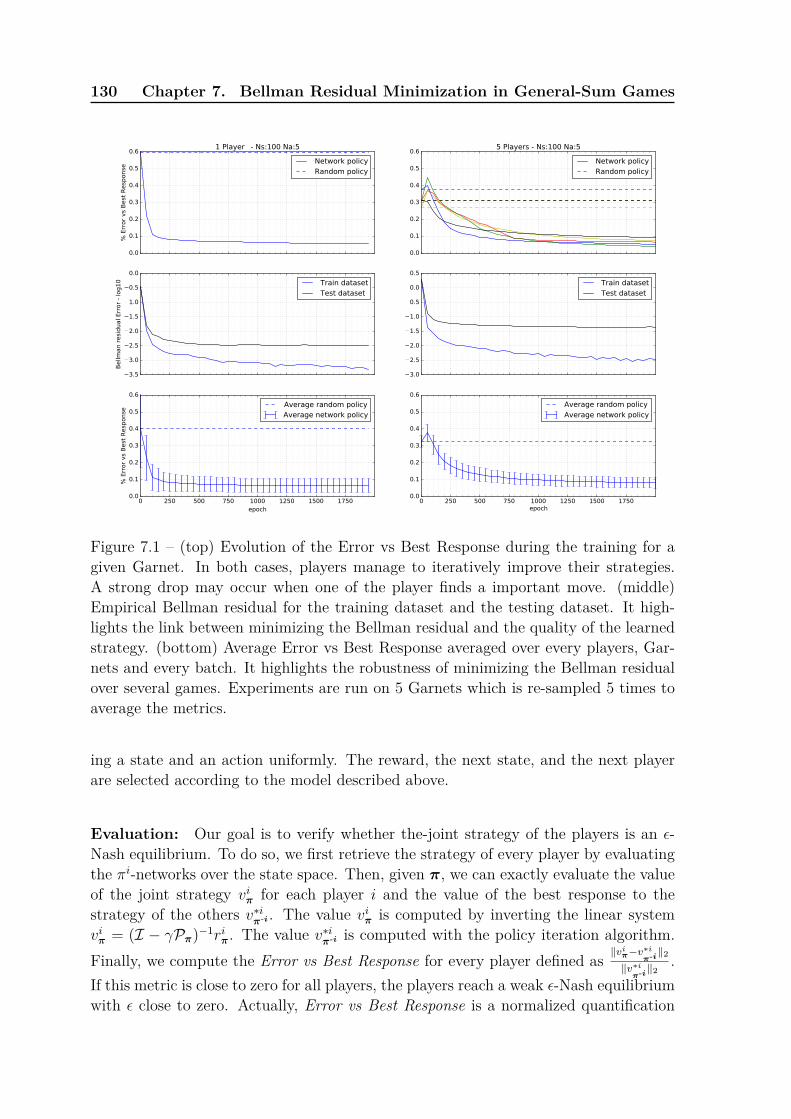
130 Chapter 7. Bellman Residual Minimization in General-Sum Games
0.0
0.1
0.2
0.3
0.4
0.5
0.6
% E
rror
vs
Best
Resp
onse
1 Player - Ns:100 Na:5
Network policyRandom policy
0.0
0.1
0.2
0.3
0.4
0.5
0.65 Players - Ns:100 Na:5
Network policyRandom policy
3.5
3.0
2.5
2.0
1.5
1.0
0.5
0.0
Bellm
an r
esi
dual Err
or
- lo
g1
0 Train datasetTest dataset
3.0
2.5
2.0
1.5
1.0
0.5
0.0
0.5
Train datasetTest dataset
0 250 500 750 1000 1250 1500 1750epoch epoch
0.0
0.1
0.2
0.3
0.4
0.5
0.6
% E
rror
vs
Best
Resp
onse Average network policy
Average random policy
0 250 500 750 1000 1250 1500 17500.0
0.1
0.2
0.3
0.4
0.5
0.6
Average network policyAverage random policy
Figure 7.1 – (top) Evolution of the Error vs Best Response during the training for agiven Garnet. In both cases, players manage to iteratively improve their strategies.A strong drop may occur when one of the player finds a important move. (middle)Empirical Bellman residual for the training dataset and the testing dataset. It high-lights the link between minimizing the Bellman residual and the quality of the learnedstrategy. (bottom) Average Error vs Best Response averaged over every players, Gar-nets and every batch. It highlights the robustness of minimizing the Bellman residualover several games. Experiments are run on 5 Garnets which is re-sampled 5 times toaverage the metrics.
ing a state and an action uniformly. The reward, the next state, and the next playerare selected according to the model described above.
Evaluation: Our goal is to verify whether the-joint strategy of the players is an ε-Nash equilibrium. To do so, we first retrieve the strategy of every player by evaluatingthe πi-networks over the state space. Then, given π, we can exactly evaluate the valueof the joint strategy viπ for each player i and the value of the best response to thestrategy of the others v∗iπ-i . The value viπ is computed by inverting the linear systemviπ = (I − γPπ)−1riπ. The value v∗iπ-i is computed with the policy iteration algorithm.Finally, we compute the Error vs Best Response for every player defined as ‖v
iπ−v∗iπ-i‖2
‖v∗iπ-i‖2
.If this metric is close to zero for all players, the players reach a weak ε-Nash equilibriumwith ε close to zero. Actually, Error vs Best Response is a normalized quantification

5. Experiments 131
of how sub-optimal the player’s strategy is compared to his best response. It indicatesthe sub-optimality margin of the policy of a player compared to his best response whileother players keep playing the same strategies. If this metric is close to zero for allplayers, then they have little incentive to switch from their current strategy. It is anε-Nash equilibrium. In addition, we keep track of the empirical norm of the Bellmanresidual on both the training dataset and the test dataset as it is our training objective.
Training parameters: We use N -player Garnet with 1, 2 or 5 players. The statespace and the action space are respectively of size 100 and 5. The state is encoded bya binary vector. The transition kernel is built with a standard deviation σs′ of 1. Thereward function is ri(s) = 2 min(|s−si|,NS)−|s−si|)
NS(it is a circular reward function). The
reward sparsity mnoise is set to 0.5 and the reward white noise σnoise has a standarddeviation of 0.05. The discount factor γ is set to 0.9. The Q-networks and π-networkshave one hidden layers of size 80 with RELUs Goodfellow et al. (2016). Q-networks haveno output transfer function while π-networks have a softmax. The gradient descentis performed with AdamGrad Goodfellow et al. (2016) with an initial learning rate of1e-3 for the Q-network and 5e-5 for the π-networks. We use a weight decay of 1e-6.The training set is composed of 5NSNA samples split into random minibatch of size 20while the testing dataset contains NSNA samples. The neural network is implementedby using the python framework Tensorflow Abadi et al. (2015). The source code isavailable on Github (Hidden for blind review) to run the experiments.
Results: Results for 1 player (MDP) and 5 players are reported in Figure 7.1. Ad-ditional settings are reported in the Appendix-9 such as the two-player case and thetabular cases. In those scenarios, the quality of the learned strategies converges inparallel with the empirical Bellman residual. Once the training is over, the players canincrease their cumulative reward by no more than 8% on average over the state space.Therefore, neural networks succeed in learning a weak ε-Nash equilibrium. Note thatit is impossible to reach a zero error as (i) we are in the batch setting, (ii) we use func-tion approximation and (iii) we only control a weak ε-Nash equilibrium. Moreover, thequality of the strategies are well-balanced among the players as the standard deviationis below 5 points.
Our neural architecture has good scaling properties. First, scaling from 2 playersto 5 results in the same strategy quality. Furthermore, it can be adapted to a widevariety of problems by only changing the bottom of each network to fit with the staterepresentation of the problem.
Discussions: The neural architecture faces some over-fitting issues. It requires ahigh number of samples to converge as described on Figure 7.2. Lillicrap et al. (2016)introduces several tricks that may improve the training. Furthermore, we run addi-tional experiments on non-deterministic Garnets but the result remains less conclusive.Indeed, the estimators of the Bellman residuals are biased for stochastic dynamics. Asdiscussed, embedding the kernel or using kernel estimators may help to estimate prop-

132 Chapter 7. Bellman Residual Minimization in General-Sum Games
0 1 2 3 4 5 6Sampling coefficient : alpha
0.0
0.1
0.2
0.3
0.4
0.5%
Erro
r vs B
est R
espo
nse
2 Players - Ns:100 Na:5Average NetworkAverage Random
Figure 7.2 – Impact of the number of samples on the quality of the learned strategy.The number of samples per batch is computed by Nsamples = αNANS. Experimentsare run on 3 different Garnets which are re-sampled 3 times to average the metrics.
erly the cost function (Equation (7.4)). Finally, our algorithm only seeks for a singleNash-Equilibrium when several equilibria might exist. Finding a specific equilibriumamong others is out of the scope of this thesis.
6 Conclusion
In this chapter, we present a novel approach to learn a Nash equilibrium in MGs.The contributions are both theoretical and empirical. First, we define a new (weaker)concept of an ε-Nash equilibrium. We prove that minimizing the sum of differentBellman residuals is sufficient to learn a weak ε-Nash equilibrium. From this result, weprovide empirical estimators of these Bellman residuals with batch data. Finally, wedescribe a novel neural network architecture to learn a Nash equilibrium from batchdata. This architecture does not rely on a specific MG. It also scales to a high numberof players for turn taking games. Thus it can be applied to a trove of applications.
This chapter concludes this part on Bellman residual minimization. Whilst approx-imate dynamic programming was not a convincing approach to learn Nash equilibria,Bellman residual minimization seems to be a reasonable approach for general sum

6. Conclusion 133
MGs. This approach does not reduce to the existing ones in MDPs and in zero-sumtwo-player MGs. Indeed, general-sum MGs lack key properties of MDPs and zero-sumtwo-player MGs. In MDPs and in zero-sum two-player MGs only require finding thesolution of a single fixed point equation whilst an N -player general sum MG requiressolving 2N fixed point equations simultaneously.

134 Chapter 7. Bellman Residual Minimization in General-Sum Games
7 Proof of the Equivalence of Definition 2.4 and 7.1Proof of the equivalence between definition 7.1 and 2.4.
(7.1) ⇒ (2.4):If ∃v such as ∀i ∈ 1, ..., N, T iπvi = vi and T ∗iπ-ivi = vi, then ∀i ∈ 1, ..., N,
vi = viπi,π-i and vi = maxπi
viπi,π-i .
(2.4) ⇒ (7.1):if ∀i ∈ 1, ..., N, viπi,π-i = max
πiviπi,π-i ., then ∀i ∈ 1, ..., N, the value vi = viπi,π-i is
such as T iπvi = vi and T ∗iπ-ivi = vi.
8 Proof of Theorem 7.1First we will prove the following lemma. The proof is strongly inspired by previouswork on the minimization of the Bellman residual for MDPs Piot et al. (2014a).
Lemma 7.1. let p and p′ be a real numbers such that 1p
+ 1p′
= 1, then ∀v,π and∀i ∈ 1, ..., N:∥∥∥viπi∗,π-i − viπi,π-i
∥∥∥µ,p
(7.5)
≤ 11− γ
(C∞(µ, ν, πi∗,π-i)
p′p + C∞(µ, ν, πi,π-i)
p′p
) 1p′[∥∥∥T ∗iπ-iv
i − vi∥∥∥pµ,p
+∥∥∥T iπvi − vi∥∥∥p
µ,p
] 1p
,
(7.6)
where πi∗ is the best response to π-i. Meaning viπi∗,π-i is the fixed point of T ∗iπ-i. And with
the following concentrability coefficient C∞(µ, ν, πi,π-i) =∥∥∥∥∂µT (1−γ)(I−γP
πi,π-i )−1
∂νT
∥∥∥∥ν,∞
.
Proof. The proof uses similar techniques as in Piot et al. (2014a). First we have:
viπi,π-i − vi = (I − γPπi,π-i)−1(riπi,π-i − (I − γPπi,π-i)vi), (7.7)= (I − γPπi,π-i)−1(T iπi,π-ivi − vi). (7.8)
But we also have:
viπi∗,π-i − vi = (I − γPπi∗,π-i)−1(T iπi∗,π-ivi − vi),
then:
viπi∗,π-i − viπi,π-i = viπi∗,π-i − vi + vi − viπi,π-i , (7.9)= (I − γPπi∗,π-i)−1(T iπi∗,π-iv
i − vi)− (I − γPπi,π-i)−1(T iπi,π-ivi − vi),(7.10)
≤ (I − γPπi∗,π-i)−1(T ∗iπ-ivi − vi)− (I − γPπi,π-i)−1(T iπi,π-ivi − vi),(7.11)
≤ (I − γPπi∗,π-i)−1∣∣∣T ∗iπ-ivi − vi
∣∣∣+ (I − γPπi,π-i)−1∣∣∣T iπi,π-ivi − vi
∣∣∣ .(7.12)

9. Additional curves 135
Finally, using the same technique as the one in Piot et al. (2014a), we get:∥∥∥viπi∗,π-i − viπi,π-i
∥∥∥µ,p
(7.13)
≤∥∥∥(I − γPπi∗,π-i)−1
∣∣∣T ∗iπ-ivi − vi∣∣∣∥∥∥µ,p
+∥∥∥(I − γPπi,π-i)−1
∣∣∣T iπi,π-ivi − vi∣∣∣∥∥∥µ,p, (7.14)
≤ 11− γ
[C∞(µ, ν, πi∗,π-i)
1p
∥∥∥T ∗iπ-ivi − vi∥∥∥ν,p
+ C∞(µ, ν, πi,π-i)1p
∥∥∥T ∗iπ-ivi − vi∥∥∥ν,p
],
(7.15)
≤ 11− γ
(C∞(µ, ν, πi∗,π-i)
p′p + C∞(µ, ν, πi,π-i)
p′p
) 1p′[∥∥∥T ∗iπ-ivi − vi
∥∥∥pν,p
+∥∥∥T iπvi − vi∥∥∥pν,p
] 1p
.
(7.16)
Theorem 7.1 falls in two steps:∥∥∥∥∥∥∥∥∥max
πivπi,π-i − viπ
∥∥∥∥µ(s),p
∥∥∥∥∥ρ(i),p
≤ 11− γ
[max
i∈1,...,N
(C∞(µ, ν, πi∗,π-i)
p′p + C∞(µ, ν, πi,π-i)
p′p
) 1p′]
(7.17)
×[N∑i=1
ρ(i)(∥∥∥T ∗iπ-iv
i − vi∥∥∥pν,p
+∥∥∥T iπvi − vi∥∥∥p
ν,p
)] 1p
, (7.18)
≤ 21p′C∞(µ, ν)
1p
1− γ
[N∑i=1
ρ(i)(∥∥∥T ∗iπ-iv
i − vi∥∥∥pν,p
+∥∥∥T iπvi − vi∥∥∥p
ν,p
)] 1p
,
(7.19)
with C∞(µ, ν) =(
supπi,π-i
C∞(µ, ν, πi,π-i))
The first inequality is proven using lemma 1 and Holder inequality. The secondinequality falls noticing ∀πi,π-i, C∞(µ, ν, πi,π-i) ≤ sup
πi,π-iC∞(µ, ν, πi,π-i).
9 Additional curvesThis section provides additional curves regarding the training of the Network.

136 Chapter 7. Bellman Residual Minimization in General-Sum Games
0.0
0.1
0.2
0.3
0.4
0.5
0.6
% E
rror v
s Bes
t Res
pons
e
2 Players - Ns:100 Na:5Network policyRandom policy
0.0
0.1
0.2
0.3
0.4
0.5
0.6 5 Players - Ns:100 Na:5Network policyRandom policy
3.5
3.0
2.5
2.0
1.5
1.0
0.5
0.0
Bellm
an re
sidua
l Erro
r - lo
g10 Train dataset
Test dataset
3.0
2.5
2.0
1.5
1.0
0.5
0.0
0.5Train datasetTest dataset
0 250 500 750 1000 1250 1500 1750epoch
0.0
0.1
0.2
0.3
0.4
0.5
0.6
% E
rror v
s Bes
t Res
pons
e Average network policyAverage random policy
0 250 500 750 1000 1250 1500 1750epoch
0.0
0.1
0.2
0.3
0.4
0.5
0.6Average network policyAverage random policy
Figure 7.3 – (top) Evolution of the Error vs Best Response during the training for agiven Garnet. (middle) Empirical Bellman residual for the training dataset and thetesting dataset. (bottom) Average Error vs Best Response averaged over every players,Garnets and every batch. Experiments are run on 5 Garnets which is re-sampled 5times to average the metrics.

9. Additional curves 137
0.0
0.1
0.2
0.3
0.4
0.5
0.6
% E
rror v
s Bes
t Res
pons
e
1 Players - Ns:100 Na:5Random policyNetwork policy
0.0
0.1
0.2
0.3
0.4
0.5
0.6 2 Players - Ns:100 Na:5Random policyNetwork policy
0.0
0.1
0.2
0.3
0.4
0.5
0.6 5 Players - Ns:100 Na:5Random policyNetwork policy
3.5
3.0
2.5
2.0
1.5
1.0
0.5
0.0
Bellm
an re
sidua
l Erro
r - lo
g10 Train dataset
Test dataset
3.0
2.5
2.0
1.5
1.0
0.5
0.0Train datasetTest dataset
2.5
2.0
1.5
1.0
0.5
0.0
0.5Train datasetTest dataset
0 250 500 750 1000 1250 1500 1750epoch
0.0
0.1
0.2
0.3
0.4
0.5
0.6
% E
rror v
s Bes
t Res
pons
e Average random policyAverage network policy
0 250 500 750 1000 1250 1500 1750epoch
0.0
0.1
0.2
0.3
0.4
0.5
0.6Average random policyAverage network policy
0 250 500 750 1000 1250 1500 1750epoch
0.0
0.1
0.2
0.3
0.4
0.5
0.6Average random policyAverage network policy
Figure 7.4 – Tabular basis. One may notice that the tabular case works well for a 1player game (MDP). Yet, the more players there are, the worth it performs. Experi-ments are run on 5 Garnets which is re-sampled 5 times to average the metrics.
0 250 500 750 1000 1250 1500 1750epoch
0.00
0.05
0.10
0.15
0.20
0.25
0.30
0.35
0.40
% E
rror v
s Bes
t Res
pons
e
Network policyRandom policy
0 250 500 750 1000 1250 1500 1750epoch
0.10
0.15
0.20
0.25
0.30
0.35
0.40
Dist
ribut
ion
over
act
ion
Action 0Action 1Action 2Action 3Action 4
Figure 7.5 – (left)Evolution of the Error vs Best Response during the training for a givenGarnet. When the Garnet has a complex structure or the batch is badly distributed,one player sometimes fails to learn a good strategy. (right) Distribution of actions inthe strategy among the players with the highest probability. This plots highlights thatπ-networks do modify the strategy during the training

138 Chapter 7. Bellman Residual Minimization in General-Sum Games
Shared weights
SelectSelect
𝜋𝜃 𝑠′𝑆 → 𝐴
max
−γ ×
+
+
action
next player
𝑄𝜃 𝑠, 𝑎𝑆 → 𝐴
𝑄𝜃 𝑠′, 𝑏𝑆 → 𝐴
reward
state next state next state
next player
Matrices: 𝐽 x 1
Matrices: 𝐽 x 𝐴
Dot product
+× Sum, product
terms by terms
Multiplexer
B
pAY
𝑌 = 𝐴 𝑖 𝑖𝑓 𝑖 ≠ 𝑝
𝐵 𝑖(A.0) (B)
(D)
(C.1)
(E)
(H)
(G)−γ ×
(F)reward
(A.1)
(C.0)
(C.2)
Figure 7.6 – This scheme summarizes the neural architecture that learns a Nashequilibrium by minimizing the Bellman residual for turn-based games. Each playerhas two networks : a Q-network that learns a state-action value function and a π-network that learns the strategy of the player. The final loss is an empirical esti-mate of the sum of Bellman residuals given a batch of data of the following shape(s, (a1, . . . , aN), (r1, . . . , rN), s′). The equation (7.4) can be divided into key opera-tions that are described below. For each player i : first of all, in (A.0) we computeQi(s, a1, . . . , aN) by computing the tensor Qi(s,a) and then by selecting the value ofQi(s,a) (A.1) given the action of the batch. Step (B) computes the tensor Qi(s′, b)and step (C.0) computes the strategy πi(.|s′). In all Bellman residuals we need toaverage over the strategy of players Qi(s′, b). Since we focus on turn-based MGs, wewill only average over the strategy of the player controlling next state s′ (in the fol-lowing, this player is called the next player). In (C.1) we select the strategy π(.|s′)of the next player given the batch. In (C.2) we duplicate the strategy of the nextplayer for all other players. In (D) we compute the dot product between the Qi(s′, b)and the strategy of the next player to obtain Eb∼π[Qi(s′,b)] and in (E) we pickthe highest expected rewards and obtain max
bQi(s′, b). Step (F) aims at computing
maxbi
[Eb-i∼π-i [Qi(s′, bi, b-i)]
]and, since we deal with a turn-based MG, we need to select
between the output of (D) or (E) according to the next player. For all i, we either selectthe one coming from (E) if the next player is i or the one from (D) otherwise. In (G)we compute the error between the reward ri to Qi(s, a)−γmax
bi
[Eb-i∼π-i [Qi(s′, bi, b-i)]
]and in (H) between ri and γEb∼π[Qi(s′,b)]−Qi(s, a). The final loss is the sum of allthe residuals.

Part IV
Independent Learning in Games


Chapter 8
Actor-Critic Fictitious Play
This chapter contributes to filling a gap in the MARL literature by providing twoonline independent RL algorithms converging to a Nash equilibrium in multi-stagegames both in the cooperative case and the zero-sum two-player case. Those two casesused to be treated as different agendas since the seminal paper of Shoham et al. (2007)and we expect our work to serve as a milestone to reconcile them going further thannormal form games (Leslie and Collins, 2006, Hofbauer and Sandholm, 2002).
We proposed two novel on-line and decentralized algorithms inspired by actor-criticarchitectures for Markov Games, each of them working on two time-scales. Those twoalgorithms perform the same actors’ update but use different methods for the critic.The first one performs an off-policy control step whilst the second relies on a policyevaluation step. Although the actor-critic architecture is popular for its success insolving continuous action RL domains, we chose this architecture for a different reason.Our framework requires handling non-stationarity (because of adaptation of the otherplayers) which is another nice property of actor-critic architectures. Our algorithms arestochastic approximations of two dynamical systems that generalize the work of Leslieand Collins (2006) and Hofbauer and Sandholm (2002) on the fictitious play processfrom normal form games to multistage games Bošanský et al. (2016).
In the following, we first describe the necessary background in both game theoryand RL (Section 1) to introduce our first contribution, the two-timescale algorithms(Section 2). These algorithms are stochastic approximations of two continuous-timeprocesses defined in Section 3. Then, we study (in Section 3) the asymptotic behavior ofthese continuous-time processes and show, as a second contribution, that they convergein self-play in cooperative games and in zero-sum two-player games. In Section 4, ourthird contribution proves that the algorithms are stochastic approximations of the twocontinuous-time processes. Finally, we perform an empirical evaluation (in Section 5).
1 Specific BackgroundMultistage Game: We consider games that can be modeled as trees (see Fig. 8.1 inappendix). The state s is the root of the game tree and each state can be reached withsome non-zero probability with at least a deterministic joint strategy. Furthermore,we enforce the fact that once a state is visited, it can never be visited again exceptstate Ω, the end of the game. Formally, a multistage game is an MG with an initial

142 Chapter 8. Actor-Critic Fictitious Play
state s ∈ S and an absorbing state Ω ∈ S. To enforce that a state can be only visitedonce, we define an ordering bijection φ : S → 1, . . . , |S| where |S| is the cardinalof S, φ(s) = |S|, φ(Ω) = 1 and such that ∀s, s′ ∈ S × S\(Ω,Ω), φ(s) ≤ φ(s′) ⇒∀π, Pπ(s′|s) = 0. Moreover the reward in state Ω is null (meaning r(Ω, .) = 0) andno player has more than one action available in that absorbing state. Furthermore, forany state s ∈ S\s,Ω there exists a deterministic strategy π and a time t ≤ |S| suchthat P tπ(s|s) > 0. This condition means that every states can be reached from state swith at least a deterministic strategy.
12
-1
max
min
... ... ... ...
(ai,a-i)
s′ ∼ p(.|s,a)
Ω
s
Figure 8.1 – Example of a two-player zero-sum multistage game with deterministicdynamics.
1.1 Specific Operators and Value FunctionsWe define here specific best responses operators and values. Instead of using argmaxas a greedy strategy, we will use a smooth version of the argmax (i.e. a Logit choicefunction). In this subsection, we review notations introduced in Chapter 2 and defineones specific to this chapter.
Value Function and State-Action Value Function: In a γ-discounted multistagegame, (with γ ∈ (0, 1)), the value is defined as in MGs (see Section 3 of Chapter 2):
viπ(s) = E[+∞∑t=0
γtriπ(st)|s0 = s, st+1 ∼ Pπ(.|st)],
=(I + γPπ + · · ·+ γ|S|P |S|π
)riπ.

1. Specific Background 143
Note that for a multistage game, the value function is well defined even for γ = 1since the process has an absorbing state Ω where the reward function is null. Fort > |S|, we have that P tπriπ = 0 since after |S| steps (at most) the process ends upin the absorbing state Ω. We can also define a state-action value function per player,that is the value of performing action ai in state s and then following its strategy:Qiπ(s, ai) = riπ-i(s, ai) + γ
∑s′pπ-i(s′|s, ai)viπ(s′) (8.1).
Logit Choice Function: when given a choice between actions a ∈ A based onan expected value Q(a) (in the following Q(a) will be the state-action value functionQiπ(s, ai) or Q∗iσ,π-i(s, ai) defined below), it is common not to take the action that max-
imizes Q(a) but to choose suboptimal actions so as to favor exploration. One commonchoice of suboptimal actions is to pick them according to the logit choice functionBη(Q)(a) = exp(η-1Q(a))∑
aexp(η-1Q(a)) . We will write Cη(Q) = ∑
a∈AQ(a)Bη(Q)(a) the expectedoutcome if actions are taken according to the logit choice function. This definitioncan be generalized to the notion of choice probability function (see remark 8.1) andwill be written Bσ(Q) and Cσ(Q) where σ is a function in R∆A. Here ∆A is the setof distributions over actions. In the case of the logit choice function, η is linked to σthrough the following formula σ(π) = ∑
a ηπ(a) ln(π(a)).
Best Responses: If the strategy π-i of all opponents is fixed, the value of the bestresponse is v∗iσ,π-i and is recursively defined as follows (starting from Ω and going inincreasing order with respect to φ): v∗i
σ,π-i(s) = Cσ(riπ-i(s, ai)+
∑s′∈S pπ-i(s′|s, ai)v∗iσ,π-i(s′)).
From the definition of that value function, we define the corresponding Q-function:Q∗iσ,π-i(s, ai) = ri
π-i(s, ai) + γ∑s′ pπ-i(s′|s, ai)v∗iσ,π-i(s′). (8.2)
Bellman Operators: We define the two following Bellman operators on theQ-function: [
T iπQi](s, ai) = ri
π-i(s, ai) + γ∑s′ pπ-i(s′|s, ai)Ebi∼πi(.|s′)
[Qi(s′, bi)
], and
[T ∗iσ,π-iQ
i](s, ai) = riπ-i(s, ai) + γ
∑s′ pπ-i(s′|s, ai)Cσ
(Qi(s′, .)
). The value Qi
π is the fixedpoint of the operator T iπ and Q∗iσ,π-i is the fixed point of the operator T ∗iσ,π-i . Further-more, a strategy πi is greedy with respect to a Q-function Qi if T ∗iσ,π-iQi = T iπi,π-iQi.
Operators on the Value Function: we define the counterparts of those operatorson value functions as follows: [T iπvi] (s) = riπ(s) + γ
∑s′ pπ(s′|s)vi(s′) , [T iπvi] = riπ +
γPπvi and [T ∗iσ,π-iv
i] = Cσ(riπ-i(s, .) + γ
∑s′ pπ-i(s′|s, .)vi(s′)). (8.3) From these definitions,
we have the two following value functions: v∗iσ,π-i(s) = Cσ(Q∗iσ,π-i(s, .)) and viπ(s) =Ebi∼πi(.|s) [Qi
π(s, bi)].
Smooth Nash Equilibrium: The goal in this setting is to find a strategy πi for eachplayer that recursively (in increasing order with respect to function φ(.)) fulfills thefollowing condition: ∀i, Eai∼πi(.|s)
[Qiπ(s, .)
]= Cσ(Qiσ,π(s, .)). As a consequence, we have
that Q∗iσ,π-i = Qiπ and viπ = v∗iσ,π-i . Furthermore, in the case of a zero-sum two-player
game, we have viπ = −v-iπ (where v-iπ is the value function of the opponent)

144 Chapter 8. Actor-Critic Fictitious Play
2 Actor-Critic Fictitious Play
We present here our first contribution: the actor-critic fictitious play algorithm forMGs. This is an on-line and decentralized process. At each time-step n, all playersare in state sn, players choose independently an action ain according to their currentstrategy πin(.|sn) and observe independently one from another a reward signal rin =ri(sn,an). The process is decentralized, meaning players do not observe others’ actionsnor their rewards. Then, the game moves to the following state sn+1. If the processreaches the absorbing state Ω, we simply restart from the beginning (s).
Algorithm 27 On-line Actor Critic Fictitious PlayInput: An initial strategy πi0 and an initial value vi0 = 0. Two learning ratesαnn≥0, βnn≥0 satisfying assumption A 3 and an initial state s0 = s.for n=1,2,... doAgent i draws action ain ∼ πi(.|sn).Agent i observes reward rin = ri(sn,an).Every player observes the next state sn+1 ∼ p(.|sn,an).actor stepπin+1(sn, .) = (1− βn)πin(sn, .) + βnBσ(Qin(sn, .))critic stepEither an off-policy control step:Qin+1(sn, ain) = (1− αn)Qin(sn, ain) + αn
(rin + Cσ
(Qin(sn+1, .)
))Or a policy evaluation step:Qin+1(sn, ain) = (1− αn)Qin(sn, ain) + αn
(rin + Eb∼πin(.|sn+1)
(Qin(sn+1, b)
))if sn+1 = Ω thensn+1 = s.
end ifend forReturn The joint strategy π and values vi for all i.
The learning algorithm performs two updates. First, it updates the players’ strategy(actors’ update). The strategy πin+1 is a mixture between the current strategy πin andeither a local best response Bσ(Qi
πn(sn, .)) or a global best response Bσ(Q∗iσ,π-in
(sn, .)).The actors’ update is performed according to a slow timescale βn. Second, it performsthe critics’ update which evaluates the current strategy. It happens on a fast timescaleαn on which we can consider that the strategy of every player is stationary. If at theactors’ step we want to act according to a local best response dynamics, the critic stepwill perform a policy evaluation step. If we want to perform a global best responsedynamics, the critic will perform an off-policy evaluation step. Thus, at the slowtimescale, the Q-function Qi
n has almost converged to Q∗iσ,π-inor to Qi
πn . Therefore, weobtain canonically two algorithms.
In the next section, as a second contribution, we introduce the two dynamicalprocesses corresponding to these algorithms and we prove that they possess desirable

3. Fictitious play in Markov Games 145
properties (i.e. rationality and convergence in self play for zero-sum two-player andcooperative games). The proofs rely non trivial techniques to propagate the Lyapunovstability property of the Fictitious play process of these ODE on the tree structure ofthe multistage games. Then in Section 4, as a third contribution, we show formally thatthese two algorithms (Algorithm 27) are stochastic approximations of those dynamicalprocesses. This is again non-trivial as we need to prove the convergence of a two-timescale discrete scheme depending on a Markov chain.
Remark 8.1. In the previous section, we defined the logit choice function. Onecan generalize this notion with the concept of choice probability function (see Hof-bauer and Sandholm (2002)). Imagine a player is given a choice of an action a ∈ Abased on the outcome Q(a). Instead of choosing based on the outcome Q(a), healso obtains an additive random payoff εa and chooses with respect to Q(a) + εa.The vector (εa)a∈A is a positive random variable taking it’s value in R|A| and doesnot depend on Q(a). These choice probability functions allow us to get smoothBellman operators and ease the analysis of our algorithms. A choice probabilityfunction is defined as follows: Bσ(Q)(a) = P (argmaxa∈A[Q(a) + εa] = a). This defi-nition is equivalent to the following one where σ(.) is a deterministic perturbation:Bσ(Q) = argmaxπ∈∆(A)[Ea∼π[Q(a)] − σ(π)]. The function Cσ(Q) is the average valueconsidering the choice probability function Bσ(Q): Cσ(Q) =
∑a∈AQ(a)Bσ(Q)(a). This
perturbation is said admissible Hofbauer and Sandholm (2002) if for all y, ∇2σ(y) ispositive definite on R0 = z ∈ Rn : ∑j zj = 0, and if ‖∇σ(y)‖ goes to infinity as yapproaches the boundary of ∆A. For example, Bσ(Q)(a) = exp(η-1Q(a))∑
aexp(η-1Q(a)) if the σ(.)
perturbation is defined as σ(π) = ∑a ηπ(a) ln(π(a)). In that case, the noise εa follows
a Gumbel distribution. From now on, we consider that σ(.) is fixed.
3 Fictitious play in Markov GamesIn this section, we propose novel definitions for two perturbed best response dynamics inthe case of MGs. These dynamics are defined as a set of Ordinary Differential Equations(ODE) that generalizes the continuous time Fictitious play process to MSGs Hofbauerand Sandholm (2002). Then, we prove the convergence of these processes in multistagegames. To do so, we build on the work of Hofbauer and Sandholm (2002) on thestability of the Fictitious play process in normal form games. By induction on the treestructure of multistage games, we prove that our processes have stable attractors inzero-sum two-player and in cooperative multistage games. Later in Section 4, we willprove that our actor-critic algorithms track the solutions of that ODE and thus areguaranteed to converge in both settings. The first one considers a local best responsedynamics: πit(.|s) = dπt(s)[Bσ(Qi
πt(s, .))− πit(.|s)] (8.4)The second process considers a global best response:
πit(.|s) = dπt(s)[Bσ(Q∗iσ,π-i
t(s, .))− πit(.|s)] (8.5)
Remark 8.2. The distribution dπ is the stationary distribution of the Markov processdefined by s′ ∼ pπ(.|s) and if s′ = Ω, we restart the process from s. One can show that

146 Chapter 8. Actor-Critic Fictitious Play
if we start the process with a strategy π0 that gives a non-null probability for eachaction and each player, the distribution over states dπt(s) is never null since we considerthat there is at least a deterministic strategy that reaches any state. Furthermore, sincewe consider smooth best response dynamics, the smooth best response will assign toeach action some probability which is bounded away from zero (since the Q-functionare bounded). Thus, we can always consider that we will visit each state with someminimal probability (i.e. dπt(s) ≥ δ > 0).
Two properties are usually desirable for such a stochastic process which are ratio-nality and convergence in self-play Bowling and Veloso (2001). Rationality implies thatif other players converge to a stationary strategy, the learning algorithm will convergeto a best response strategy. The convergence property received many definitions in theMARL literature and usually ensures convergence of the algorithm against a class ofother algorithms or convergence in self-play. Here, we choose the later.
Rationality: For the rest of this paragraph, let us study a fixed player i. First, ifwe consider the case where other players are stationary (i.e. π-i
t = π-i), the strat-egy of player i will converge to Bσ(Q∗iσ,π-i(s, .)) for the second process Eq. (8.5) (sinceBσ(Q∗i
σ,π-i(s, .))does not depend on πit the solution of the second process converges expo-nentially toward the best response strategy). For the first process, let us show that ifthe strategy πi follows the dynamics described by (8.4), it converges to a best responsestrategy. The proof of this property requires the following two technical lemmas.
(T, δ)-perturbation: Let us consider the following ODE where h(.) : Rn → Rn is aLipschitz continuous function: z(t) = h(z(t)) (8.6)
We consider the case where ODE (8.6) has an asymptotically stable attractor setJ . A bounded measurable function y(.) : R+ → RN is a (T, δ)-perturbation of (8.6)(T, δ > 0) if there exist 0 = T0 < T1 < T2 < · · · < Tn with Ti+1 − Ti ≥ T and solutionszj(t), t ∈ [Tj, Tj+1] of (8.6) for all j ≥ 0 such that sup
t∈[Tj ,Tj+1]‖zj(t) − y(t)‖ < δ. The
following technical lemma can be proved Borkar (1997b).
Lemma 8.1. Given ε, T > 0, there exists a δ > 0 such that for δ ∈ (0, δ), every(T, δ)-perturbation of Eq. (8.6) converges to J ε (def: the ε-neighborhood of J).
The next lemma is used all over this section. It proves that if, instead of followinga given process x(t) = f (x(t)), one follows a perturbed version of that process y(t) =ft (y(t)) one converges to the set of stable equilibria of the unperturbed process if ft(.)converges toward f(.).
Lemma 8.2. Let’s study the two following ODE x(t) = f (x(t)) and y(t) = ft (y(t))and let’s assume that lim sup ‖f(.)− ft(.)‖ → 0 uniformly. Furthermore, let’s assumethat f is Lipschitz continuous. Then, any bounded solution of y(t) = ft (y(t)) convergesto the set of attractors of x(t) = f (x(t)).

3. Fictitious play in Markov Games 147
Proof. The full proof of this lemma is left in appendix 7. It shows that all boundedsolutions of the time dependent ODE is a (T, δ)-perturbation of the other ODE.
Now, we show that if player i follows the direction given by the local best responsedynamics Eq. (8.4), it converges to a best response to π-i.
Proposition 1. In any game, if the strategy π-i of the opponents is fixed, the pro-cess (8.4) converges to a best response.
Proof. The proof of that property is left in appendix 10
Now, let’s consider the case where the strategy of other players π-it converges to a
stationary strategy π-i. In that case, one can show that, for a fixed i, the solutions ofODE (8.4) and (8.5) are the same as if π-i
t was fixed.
Proposition 2. If π-it → π-i, then the solutions of ODE (8.4) and (8.5) are the same
as the one of:
πit(.|s) = dπit,π-i(s)[Bσ(Qiπit,π-i(s, .))− πit(.|s)] and πit(.|s) = dπit,π-i(s)[Bσ(Q∗iσ,π-i(s, .))− πit(.|s)]
Proof. The proof of that property is left in appendix 11
Thus, if all other players converge to a stationary strategy, the strategy of player iconverges to a best response to π-i.
Convergence in Multistage Games: Concerning the convergence in self-play ofthose two fictitious play processes, one must first be aware that they will not convergein all multistage games. Even in normal form games, the fictitious play process isknown to be unstable in some cases. For example, the fictitious play process is knownto oscillate in some two-player games Shapley (1964). More surprisingly, Hart and Mas-Colell (2003) proved in the case of normal form games that there exists no uncoupleddynamics which guarantees Nash convergence. In their paper, they consider dynamicsfor each player which only depends on its own reward and possibly on the strategy ofall players. They present an example in which this class of dynamical systems has nostable equilibrium. We were able to prove the convergence of our process in the caseof zero-sum two-player and cooperative multistage games.
Proposition 3. In a zero-sum two player multistage game, the process (8.4) and theprocess (8.5) converge to a smooth Nash equilibrium π.
Proof. The proof of that property is left in appendix 12
Remark 8.3. Proposition 3 can be adapted to study the cooperative case (i.e. whenplayers receive the same reward ∀i, j ri(s,a) = rj(s,a)). The proof in the cooperativecase also works by induction. The corresponding proposition and proof can be foundin the appendix 9.

148 Chapter 8. Actor-Critic Fictitious Play
4 Stochastic Approximation with Two-TimescaleIn this section, we provide a novel stochastic approximation theorem taking advantageof two independent techniques. First, we use two timescales because the process weare studying (defined on the strategy of each player called the actor) has a complexdependency on the strategy of all players through the Q-function (the critic). In anon-line setting, one can’t have access to the Q-function of a given strategy (either Qi
π
or Q∗iσ,π-i) as it is an asymptotic solution of the critic process. Thus formally, we lookfor an asymptotically stable solution of y(t) = g(µ(y(t)), y(t)) (actors’ update) whereµ(y) is the stable solution of another process x(t) = f(x(t), y)(critics’ update). Inour case µ(y) is either Qi
π or Q∗iσ,π-i , y is the strategy and x the action-value function.Instead of waiting until the subroutine converges (the critic part) to iterate over themain routine (the actor part), Borkar (1997b) gives an elegant solution to that classof problems by using two timescales to update simultaneously xn and yn. The processxn will be updated according to a "fast" timescale αn. On that timescale, yn behavesas if it was stationary and thus, xn is an estimate of µ(yn) (i.e. ‖µ(yn) − xn‖ → 0).The process yn will move on a "slower" timescale βn. On that slower timescale, onecan treat the process xn as µ(yn) and thus, yn will converge to a stable solution ofy(t) = g(µ(y(t)), y(t)).
Second we use an averaging technique. Our process is on-line and follows a Marko-vian dynamics controlled by the policy πn. All policies and Q-functions are onlyupdated on state sn. Thus, the two processes xn and yn also depend on a Markovprocess Zn controlled by yn. Again, Borkar (2006) shows that, in the case of a simpletimescale, the process yn+1 = yn+αnf(yn, Zn) tracks the solution of y(t) = f(y(t), dy(t))where f(y(t), dy(t)) is the average of f over the stationary distribution of Zn (the dis-tribution dy). Formally, f(y, dy) = ∑
z∈Z f(y, z)dy(z). In our case, we need to studythe following recursion:
xn+1 = xn + αnf(xn, yn, Zn), (8.7)yn+1 = yn + βng(xn, yn, Zn), (8.8)
Where:
Assumption 1. Functions f and g are jointly continuous in their arguments andLipschitz in their two first arguments uniformly with respect to the third.
Assumption 2. The controlled Markov process Zn takes its value in a discrete spaceZ controlled by variable yn. The variable Zn+1 follows the kernel p(.|Zn, yn) which isuniformly continuous in yn. Furthermore, let us suppose that if yn = y, the Markovchain Zn has a unique invariant distribution dy(.).
We note f(x, y, dy) = ∑z∈Z f(x, y, z)dy(z) the function f averaged over the station-
ary distribution of the Markov chain defined in the previous assumption. Similarly,g(x, y, dy) = ∑
z∈Z g(x, y, z)dy(z).

4. Stochastic Approximation with Two-Timescale 149
Assumption 3. The sequences αnn≥0 and βnn≥0 are two positives decreasing step-size sequences satisfying: ∑
n≥0αn = ∑
n≥0βn = ∞, ∑
n≥0α2n < ∞, ∑
n≥0β2n < ∞ and βn =
o(αn)
Assumption 4. We need supn‖xn‖ <∞ and sup
n‖yn‖ <∞
Assumption 5. For any constant y, the ODE: x(t) = f(x(t), y, dy), has a globallyasymptotically stable equilibrium µ(y). That stable equilibrium µ(.) is a Lipschitz con-tinuous function.
Assumption 6. The ODE y(t) = g(µ (y(t)) , y(t), dy(t)
)has a globally asymptotically
stable equilibrium y∗
Theorem 8.1. (xn, yn)→ (µ(y∗), y∗) almost surely (a.s.).
Analysis of Actor-Critic Fictitious Play: The analysis of our two algorithms isa direct application of the previous theorem and is left in appendix (App. 13). In anutshell, the critic Qn is updated on a fast timescale (i.e. xn) and we will prove that it’srecursion satisfy assumption A 1, A 2, A 3, A 4, and A 5. The actor πn is updated on aslow timescale (i.e. yn) and satisfy assumption A 1, A 2, A 3, A 4, and A 6. Thanks tothe use of choice probability function, assumption A 1 is satisfied on the slow timescalesince a choice probability function is lipschitz with respect to the Q-function. Thetwo on-line algorithms we present here (Algo 27) are stochastic approximations of thetwo dynamical systems (8.4) and (8.5). In an on-line setting, the interaction betweenplayers proceeds as follows. At a step n, players are in state sn and individually take anaction ain ∼ πin(.|sn). Each of them receives a reward ri(sn, a1
n, . . . , aNn ) and the process
moves from state sn to state sn+1 ∼ p(.|sn, a1n, . . . , a
Nn ). In addition, we consider the
controlled Markov process Zn = (sn, a1n, . . . , a
Nn , sn+1) (controlled by the strategy πn).
Finally, if sn+1 = Ω, we restart from state s and Zn+1 = (s, . . . ). We define thefollowing two-timescale processes (with αn and βn defined as in A 3):
πin+1 = πin + βn1sn1>sn[Bσ(Qin(sn, .))− πin(.|sn)
](8.9)
And:
Qin+1 = Qin + αn1(sn,ain)1>(sn,ain)
[ri(sn,an) + Cσ
(Qin(sn+1, .)
)−Qin(sn, ain)
](8.10)
Or:
Qin+1 = Qin + αn1(sn,ain)1>(sn,ain)
[ri(sn,an) + Ebi∼πi(.|sn+1)
(Qin(sn+1, b
i))−Qin(sn, ain)
](8.11)
Assumption A 1 and assumption A 2 are verified. Regarding assumption A 4, thestrategy πin is obviously bounded since it remains in the simplex. If Qi
0 = 0, the state-action value function is bounded as follows ‖Qi
n(s, a)‖ ≤ φ(s)Rmax (this can be shownby recursion). The two faster processes(Eq. (8.22) and (8.23)) track the two followingODE:
Qit(s, ai) = dπ(s)πi(.|s)([T ∗iσ,π-iQ
it
](s, ai)−Qit(s, ai)
)

150 Chapter 8. Actor-Critic Fictitious Play
AndQit(s, ai) = dπ(s)πi(.|s)
([T iπQ
it
](s, ai)−Qit(s, ai)
)Those two equations admit as an attractor Q∗iσ,π-i and Qi
π. Then, the strategy recur-sion follows either ODE (8.4) (if the subroutine is defined by Eq. (8.23)) or ODE (8.5)(if the subroutine is defined by (8.22)).
5 Experiment on AlesiaThe game of Alesia is described in Chapter 3. This game is challenging in manyaspects. First, rewards are sparse and are received at the end of the game. Furthermore,strategies need to be stochastic Buro (2004), Bošanský et al. (2016). The performancecriterion used to compare algorithms is the difference of the value of the joint strategyviπ(s) and the value of the best response vi0,π-i(s) without any perturbation σ (i.e.σ = 0)
0 500000 1000000 1500000 2000000 2500000Iterations
0.0
0.2
0.4
0.6
0.8
1.0
Per
form
ance
ACFP control player 0
ACFP control player 1
ACFP evaluation player 1
ACFP evaluation player 0
Figure 8.2 – Performance of the strategy πi (y-axis) along iterations (x-axis).
We ran experiments for a game with learning rates of the form αn = α0aαaα+nbα and
βn = β0aβ
aβ+nbβ. We used a logit choice function with η decaying with the number of
iterations ηn = η0aηaη+n . The two step-sizes αn and βn were chosen to satisfy the conditions
of Theorem 8.1. The experiments were ran with an initial budget of N = 10 and aboard of size K = 3. The step-size parameters were (α0, aα, bα) = (0.1, 104, 0.8),

5. Experiment on Alesia 151
0.0 0.2 0.4 0.6 0.8 1.0 1.2 1.4Iterations 1e7
0.0
0.2
0.4
0.6
0.8
1.0P
erfo
rman
ce
ACFP control player 0
ACFP control player 1
Figure 8.3 – Performance of the strategy πi (y-axis) along iterations (x-axis).
(β0, aβ, bβ) = (0.01, 104, 1.0) and (η0, aη) = (0.1, 106). The results are displayed infigure 8.2 and shows that both algorithms learn a strategy that tend to be closerto its own best response over learning (meaning that both algorithms learn a Nashequilibrium). An empirical finding is that ACFP with a control critic converges fasterthan the one with a policy evaluation critic on that game.
Function approximation: We also ran these experiments with function approx-imations both on the strategy and on the Q-function. The main issue in Alesia isthat the number of actions available to each player depends on the remaining bud-get of the player. For each player, we aggregated states for which the budget of theplayer is fixed. The aggregated states are consecutive states with respect to the bud-get of the other players’. The results reported in Figure 8.3 show that our methodis robust to this form of function approximation. We ran experiment with an initialbudget of N = 15 on which the algorithm was able to learn a minimax strategy. Thestep-size parameters were (α0, aα, bα) = (0.1, 105, 0.9), (β0, aβ, bβ) = (0.01, 105, 1.0) and(η0, aη) = (0.05, 108).

152 Chapter 8. Actor-Critic Fictitious Play
6 ConclusionThis chapter explores two independent RL algorithms that provably converge to Nashequilibria in zero-sum MSGs and in cooperative MSGs. This work studies extensions ofthe Fictitious play process from normal form games to MSGs. Compared to previousfamilies of methods (Bowling and Veloso, 2001, Littman, 1994), these algorithms canbe applied to a larger number of settings without heuristics and without knowing theopponents actions. The main contributions were algorithmic and theoretical but wealso proposed an empirical evaluation that provides good evidence that our methodsare applicable to real problems and could scale up thanks to function approximation.
Several interesting research paths remain to be explored. The first is the studyof the stability of the two dynamical processes in MGs. The proof given for MSGspropagates the convergence property from the end of the game to the initial state.Since MGs have a graph structure, this technique can’t be applied. Thus, other stabilityarguments must be found to ensure convergence in MGs. The second research pathcould be to further study the use of function approximation. Whilst there is a wideliterature dealing with the off-policy evaluation part or the off-policy control (Watkinsand Dayan, 1992), the update of the strategy using general function approximationremains challenging. The main issue is that the strategy space should support convexcombination with a best response. The convex combination of the strategy and thebest response could be fitted at each iteration using a classification neural network.

7. Proof of Lemma 8.2 153
7 Proof of Lemma 8.2Lemma 8.2: Let’s study the two following ODE x(t) = f (x(t)) and y(t) = ft (y(t))and let’s assume that lim sup ‖f(.)− ft(.)‖ → 0 uniformly. Furthermore, let’s assumethat f is Lipschitz continuous. Then, any solution of y(t) = ft (y(t)) converges to theset of attractors of x(t) = f (x(t)).
Proof. let us fix t such as for all T > 0, ‖f(.)− ft+T (.)‖ ≤ ε. if x(t) = y(t), then:
x(t+ T )− y(t+ T ) =t+T∫t
[f(x(τ))− f(y(τ))] dτ +t+T∫t
[f(y(τ))− fτ (y(τ))] dτ (8.12)
‖(x− y)(t+ T )‖ ≤t+T∫t
‖f(x(τ))− f(y(τ))‖dτ +t+T∫t
‖f(y(τ))− fτ (y(τ))‖dτ (8.13)
≤ Kt+T∫t
‖(x− y)(τ)‖dτ + Tε (8.14)
Let’s write g(T ) = ‖(x− y)(t+ T )‖. We have g(T ) ≤ KT∫0g(τ)dτ + Tε
Let’s write h(T ) = Tε+KT∫0g(τ)dτ+ ε
Kand h′(T ) = ε+Kg(T ) ≤ ε+K(h(T )− ε
K) ≤
Kh(T )With the differential form of the Grönwall lemma:
h(δ) ≤ h(0) exp(KT ) = ε
Kexp(KT )
And we have ‖(x− y)(t+ T )‖ = g(T ) ≤ εK (exp(KT )− 1)
This inequality means that, given T , for all δ we can choose t0 large enough suchthat any trajectory of y(t) = ft0+t (y(t)) is a (T, δ)-perturbation of x(t) = f (x(t)).Then, lemma 8.1 concludes the proof.
8 Proof of Theorem 8.1
xn+1 = xn + αnf(xn, yn, Zn), (8.15)yn+1 = yn + βng(xn, yn, Zn), (8.16)
Where:A 1. Functions f and g are jointly continuous in their arguments and Lipschitz in
their two first arguments uniformly with respect to the third,A 2. The controlled Markov process Zn takes its value in a discrete space Z con-
trolled by variable yn. The variable Zn+1 follows the transition kernel p(.|Zn, yn) whichis uniformly continuous in yn. Furthermore, let us suppose that if yn = y, the Markovchain Zn has a unique invariant distribution dy(.).

154 Chapter 8. Actor-Critic Fictitious Play
From now on, we define f(x, y, dy) = ∑z∈Z
f(x, y, z)dy(z) which is the function f
averaged over the stationary distribution of the Markov chain defined in the previousassumption. Similarly, g(x, y, dy) = ∑
z∈Zg(x, y, z)dy(z).
A 3. The sequences αnn≥0 and βnn≥0 are two positives decreasing step-sizesequences satisfying: ∑
n≥0αn = ∑
n≥0βn =∞, ∑
n≥0α2n <∞, ∑
n≥0β2n <∞ and βn = o(αn)
A 4. We need supn‖xn‖ <∞ and sup
n‖yn‖ <∞
A 5. For any constant y, the ODE:
dx(t)dt
= f(x(t), y, dy), (8.17)
has a globally asymptotically stable equilibrium µ(y). That stable equilibrium µ(.) is aLipschitz continuous function.
A 6. The ODE:
dy(t)dt
= g(µ (y(t)) , y(t), dy(t)
)(8.18)
has a globally asymptotically stable equilibrium y∗
Theorem 8.1. (xn, yn)→ (µ(y∗), y∗) almost surely (a.s.).
Proof. First, rewrite Eq. (8.8) as:
yn+1 = yn + αn
[βnαng(xn, yn, Zn)
].
Since the function g is Lipschitz in the two first arguments (A 1), since Z is discrete(A 2) and since xn and yn are bounded (A 4), then we have that βn
αng(xn, yn, Zn) → 0
a.s.. Then from corollary 81 of chapter 6.3 of Borkar (2009) (first presented in (Borkar,2006)) it follows that (xn, yn) converges to an internally chain transitive invariant setof the ODE y(t) = 0 and x(t) = f(x(t), y(t), dy(t)). In other words, ‖xn − µ(yn)‖ → 0a.s..
Second, let’s write (8.8) as:
yn+1 = yn + αn[g(µ(yn), yn, Zn) + (g(xn, yn, Zn)− g(µ(yn), yn, Zn))
]. (8.19)
Since g(., ., .) is Lipschitz in the two first variables uniformly with respect to the thirdone, we have that ‖g(xn, yn, Zn) − g(µ(yn), yn, Zn)‖ ≤ K‖xn − µ(yn)‖ (for some K).Then Eq. (8.8) can be rewritten as:
yn+1 = yn + αn[g(µ(yn), yn, Zn) + εn
], (8.20)
where εn → 0 a.s.. Again, from corollary 8 of chapter 6.3 of Borkar (2009), we havethat yn → y∗ and xn → µ(y∗)
1As written in chapter 2 Borkar (2009) in all stochastic approximation scheme studied in the book(except those in chapter 9) can be added a noise εn that converges to 0 a.s.

9. Convergence in Cooperative Multistage Games 155
9 Convergence in Cooperative Multistage Games
In a cooperative game (as defined in (Busoniu et al., 2008)), the reward signal is asfollows: ∀s, i, j ri(s,a) = rj(s,a)). Thus we have the property that ∀s, i, j viπ(s) =vjπ(s)
Proposition 4. In a cooperative two player multistage game, the process (8.4) andthe process (8.5) converge to a smooth Nash equilibrium π.
Proof. The proof of this result works again by induction on the set Sn = s ∈ S|φ(s) ≤n. Let’s suppose that for all states s in Sn, the process converges to a smooth Nashequilibrium. This means that for all states in s ∈ Sn and for all players i, the strategiesπit(.|s) converge to πi(.|s) such as viπ(s) = v∗iσ,π-i(s). We also have that ∀i, j viπ(s) =vjπ(s).
Let s be the state such that φ(s) = n+ 1. Then, we define:
M i(s, ai,a-i) = ri(s, ai,a-i) +∑s′∈S
p(s′|s, ai,a-i)viπ(s′)
M it (s, ai,a-i) = ri(s, ai,a-i) +
∑s′∈S
p(s′|s, ai,a-i)viπt(s′)
And:M∗it (s, ai,a-i) = ri(s, ai,a-i) +
∑s′∈S
p(s′|s, ai,a-i)v∗iσ,π-i
t(s′)
Since the strategy πit(.|s) converges to πi(.|s), we have viπt(s) and v∗iσ,π-i
t(s) that con-
verges to viπ(s) for all s ∈ Sn and finally M it (s, ai,a-i) and M∗i
t (s, ai,a-i) converges toM i(s, ai,a-i). Then, lemma 8.2 and results of convergence of stochastic fictitious playfor N -player potential games from Hofbauer and Sandholm (2002) guarantees that theprocess in state s will converge to a smooth Nash equilibrium of the normal form gamedefined by M i(s, ai,a-i). Finally, we have viπ(s) = v∗iσ,π-i(s) and ∀i, j viπ(s) = vjπ(s).
10 Proof of proposition 1
Proof. We prove the result by induction on the set Sn = s ∈ S|φ(s) ≤ n. First,the property is true in state Ω since by definition, there is only one action availableper player. Suppose that for all s ∈ Sn, the process converges to a best response (i.e.viπ(s) = v∗iσ,π-i). Let s be the state of order n+1 (i.e. φ(s) = n+1). From the definitionof the Q-function (Eq. (8.1) and (8.2)), we have that in s the Qi
πit,π-i(s, .) converges to
Qiπ(s, .) uniformly over the actions. Moreover, since for all s ∈ Sn, viπ(s) = v∗iσ,π-i we
have that Qiπ(s, .) = Q∗iσ,π-i(s, .). From lemma 8.2, we get the convergence of πi(.|s) to
a best response if the distribution dπ is non-null in all states (see remark 8.2).

156 Chapter 8. Actor-Critic Fictitious Play
11 Proof of Proposition 2
Proof. The proof comes from the fact that Bσ
(Qiπi,π-i
t(s, .)
)converges to
Bσ
(Qiπi,π-i(s, .)
)uniformly with respect to πi (since the Q-function is polynomial in
π and Bσ (.) is Lipschitz with respect to the Q-function. Moreover, since the statespace is finite, simple convergence imply the uniform convergence) and the fact thatBσ
(Qiπi,π-i(s, .)
)is Lipschitz with respect to πi.
12 Proof of Proposition 3Proof. The proof of this result works by induction on the set Sn = s ∈ S|φ(s) ≤ n.Again, the property is true in state Ω. Let’s suppose that for all states s in Sn, theprocess converges to a smooth Nash equilibrium. This means that for all states ins ∈ Sn and for all players i, the strategies πit(.|s) converge to πi(.|s) such as viπ(s) =v∗iσ,π-i(s). We also have that viπ(s) = −v-iπ(s).
Let s be the state such that φ(s) = n+ 1. Then, we define:
M i(s, ai,a-i) = ri(s, ai,a-i) +∑s′∈S
p(s′|s, ai,a-i)viπ(s′)
M it (s, ai,a-i) = ri(s, ai,a-i) +
∑s′∈S
p(s′|s, ai,a-i)viπt(s′)
And:M∗it (s, ai,a-i) = ri(s, ai,a-i) +
∑s′∈S
p(s′|s, ai,a-i)v∗iσ,π-i
t(s′)
Since the strategy πit(.|s) converges to πi(.|s), we have viπt(s) and v∗iσ,π-i
t(s) that con-
verges to viπ(s) for all s ∈ Sn and finally M it (s, ai, a-) and M∗i
t (s, ai, a-) converges toM i(s, ai, a-). Then, lemma 8.2 and results of convergence of stochastic fictitious playfrom Hofbauer and Sandholm (2002) guarantees that the process in state s will con-verge to a smooth Nash equilibrium of the normal form game defined by M i(s, ai,a-i).Finally, we have viπ(s) = v∗iσ,π-i(s) and viπ(s) = −v-iπ(s).
13 Analysis of Actor-Critic Fictitious PlayThe two on-line algorithms we present here (Algo 27) are stochastic approximationsof the two dynamical systems (8.4) and (8.5). In an on-line setting, the interactionbetween players proceeds as follows. At a step n, players are in state sn and individuallytake an action ain ∼ πin(.|sn). Each of them receives a reward ri(sn, a1
n, . . . , aNn ) and
the process moves from state sn to state sn+1 ∼ p(.|sn, a1n, . . . , a
Nn ). In addition, we
consider the controlled Markov process Zn = (sn, a1n, . . . , a
Nn , sn+1) (controlled by the
strategy πn). Finally, if sn+1 = Ω, we restart from state s and Zn+1 = (s, . . . ). Wedefine the following two-timescale processes (with αn and βn defined as in A 3):
πin+1 = πin + βn1sn1>sn[Bσ(Qin(sn, .))− πin(.|sn)
](8.21)

14. On the Guarantees of Convergence of OFF-SGSP and ON-SGSP 157
And:
Qin+1 = Qin + αn1(sn,ain)1>(sn,ain)
[ri(sn,an) + Cσ
(Qin(sn+1, .)
)−Qin(sn, ain)
](8.22)
Or:
Qin+1 = Qin + αn1(sn,ain)1>(sn,ain)
[ri(sn,an) + Ebi∼πi(.|sn+1)
(Qin(sn+1, b
i))−Qin(sn, ain)
](8.23)
Assumption A 1 and assumption A 2 are verified. Regarding assumption A 4, thestrategy πin is obviously bounded since it remains in the simplex. If Qi
0 = 0, the state-action value function is bounded as follows ‖Qi
n(s, a)‖ ≤ φ(s)Rmax (this can be shownby recursion). The two faster processes(Eq. (8.22) and (8.23)) track the two followingODE:
Qit(s, ai) = dπ(s)πi(.|s)([T ∗iσ,π-iQ
it
](s, ai)−Qit(s, ai)
)And
Qit(s, ai) = dπ(s)πi(.|s)([T iπQ
it
](s, ai)−Qit(s, ai)
)Those two equations admit as an attractor Q∗iσ,π-i and Qi
π. Then, the strategy recur-sion follows either ODE (8.4) (if the subroutine is defined by Eq. (8.23)) or ODE (8.5)(if the subroutine is defined by (8.22)).
14 On the Guarantees of Convergence of OFF-SGSP and ON-SGSP
The main contribution to the field of MARL related to our work is the paper of Prasad& al Prasad et al. (2015). These algorithms are not decentralized but one of them,ON-SGSP, is an on-line and model-free algorithm. This paper proposes two algorithmsOFF-SGSP and ON-SGSP which are stochastic approximations of a dynamical systemdescribed in section 8. The authors claims that these algorithms converges to a Nashequilibrium of the game. The proof of the stability given in lemma 11 is wrong. In thefollowing we point out the issue with this proof.
Using their notations:
• G is the set of Nash equilibrium (the feasible set of the optimization problem),
• K is the limit set of the dynamical system (and G ⊂ K)
• K1 is the set of limits points of the dynamical system which are Nash equilibriumK ∩G
• K2 is the complementary of K1 in K (i.e. K2 = K\K2)

158 Chapter 8. Actor-Critic Fictitious Play
Lemma 11 shows that K2 contains only unstable equilibrium and conclude that bothprocesses converges to K1 and thus to a Nash equilibrium since K1 is not empty (thisfact is proven early in the paper).
Unfortunately, that proof contains a mistake. The proof proceeds as follows: Theyshow that if π∗ ∈ K2 then there exists ai,x and i such that gix,ai(viπ, π−i) > 0 andthey conclude that consequently ∂f(vπ ,π)
∂πi< 0. However, there is no direct link between
the sine of gix,ai(viπ, π−i) and∂f(vπ ,π)∂πi
since f(vπ, π) =N∑i=1
∑x∈S
∑z∈Ai(x)
πi(x, z)gix,z(viπ, π−i).
This imply that both processes might converge in K2 (i.e. not to a Nash equilibrium).

Part V
Conclusions and Future Work


1. Conclusion 161
1 Conclusion
This thesis is devoted to the study of learning in games from interaction data. Weconsider that the interaction can be modelled as a Markov Game (MG). This modelis a generalization of the Markov Decision Process to the multi-agent setting and ageneralization of normal form games to multi-state models. We studied two kinds ofproblems. The first one is the problem of learning from batch data, meaning thatthere is no way to collect new interaction data from the model. The second one isindependent reinforcement learning where each agent plays independently one from another without knowing the others behaviour.
In part II, we extend several ADP techniques from MDPs to zero-sum two-playerMGs. In Chapter 3 we extend known ADP bounds for zero-sum two-player MGsfrom the L+∞-norm to the Lp-norm. Those ADP bounds are consistent with previousanalysis of modified policy iteration in MDP. Based on these results, we propose anon-parametric batch algorithm to learn Nash equilibria in zero-sum two-player MGs.We tested this approach on the game of Alesia and Chapter 4 explores the use ofnon-stationary strategies to improve the guarantees of Chapter 3. To do so, we de-fined extensions of most ADP algorithms for zero-sum two-player MGs to the use ofnon-stationary strategies. These non-stationary algorithms improve both theoreticallyand empirically their stationary counterpart. The main improvement is to reduce theγ-sensitivity of the contribution of the error from O
(1
(1−γ)2
)to O
(1
(1−γ)(1−γm)
). Fur-
thermore, whilst the value iteration algorithm enjoys the worst guarantees, it is the onethat performs the best in practice on randomly generated zero-sum two-player MGs.Chapter 5 investigates the use of non-stationary strategies in general-sum MGs as wassuggested in previous work (Zinkevich et al., 2006). We prove that the γ-sensitivity ofvalue iteration in general-sum MGs is improved by the use of non-stationary strategiesbut that it can’t match the performance of value iteration in MDPs or in zero-sumtwo-player MGS. In the case of general-sum games, the only factor that counts is thelength of the cycle and not the number of iterations.
Part III explores the Bellman residual approach to solve MDPs, zero-sum two-player MGs and general-sum MGs. In Chapter 6, we proved that a lot of existingbatch algorithms to solve MDPs and zero-sum two player MGs could be seen as aNewton’s method on some Bellman residuals. We leveraged this link and proposedthe use of quasi-Newton methods to improve convergence at a small computation cost.Empirical evaluation on randomly generated MDPs and zero-sum two-player MGs showimprovement both in stability and performance of our method compared to existingones. However, this method can’t be applied directly to general sum games. The nextchapter (Chapter 7) generalizes this Bellman residual approach to general-sum MGs.This method relies on the minimization of two Bellman residuals per player and doesnot reduce to the one for MDPs and zero-sum two-player MGs. The minimizationof the Bellman residual is not guaranteed. However, having a small Bellman residualguarantees having an ε-Nash equilibrium. This approach was empirically investigatedon randomly generated MGs and shows promising results.

162
Part IV (Chapter 8) studies another scenario. Instead of being given a fixed amountof data we study an online learning problem. Here players must learn while they playin an independent manner. We proposed an independent RL algorithm that provablyconverges to zero-sum two-player Multi-Stage Games (MSGs) and cooperative MSGsand tested with function approximation.
2 Future WorkThis thesis mainly contributes to the problem of learning from batch data and thealgorithms we created and studied are based on Approximate Dynamic Programmingand Bellman Residual Minimization. These approaches could be extended in othersettings as in the MDP literature.
The first part of this dissertation studies batch learning using Approximate dynamicprogramming. But when a generative model of the game is provided, many otherapproaches can be used to perform each iteration of the inner loop of AGPI-Q. Thisinner loop is required to provide an approximate solution of a finite horizon MDP oflength m. Using batch data restricts the number of possible methods (we only usedapproximate value iteration to solve that part). When a generative model of the gameis provided, one can use a vast amount of methods. For instance, one could use MonteCarlo tree search to evaluate the best response of the computation.
We have seen in Chapter 3 that the use of value iteration gave the best asymp-totic performance but that early convergence could be improved using large m. In thatchapter, we suggest using large m at the beginning and reducing it after a while. Chap-ter 4 suggests using non-stationary strategies to improve the asymptotic performance ofADP methods. The value iteration algorithm using non-stationary strategies that hadthe best asymptotic performance but the early convergence is slowed down comparedto stationary algorithms. Adapting AGPI-Q to the use of non-stationary strategiescould improve early convergence while getting the same asymptotic performance.
In Chapter 6 we propose using a Bellman residual approach to learn from batchdata. We proved that using quasi Newton methods on a Bellman residual is more stableand more accurate than using LSPI or BRMPI. These methods are hardly comparableto approximate dynamic programming methods in theory but an exhaustive empiricalcomparison can still be done and building a large benchmark of simultaneous moveMGs where using stochastic strategies is compulsory, would definitely be a valuablecontribution to that field of research.
We proved that LSPI could be improved using quasi Newton methods. And LSPIhas been adapted to the online setting. In MDPs and in zero-sum two-player MGs,it could be interesting to investigate whether or not the use of second order methodscould be used online to solve MGs. Many advances in stochastic second order methodshave been made in recent years and it could be interesting to investigate its applicationto online learning in MDPs and in zero-sum two-player MGs.
In Chapter 7 we have generalized the Bellman residual approach to general-sumMGs but this method hardly scales when the actions are taken simultaneously. Future

2. Future Work 163
work in this direction should focus on whether or not it is possible to only get adependency on the action of one player instead of the joint action. One idea could beto use importance sampling if the policy used to collect the data is known.
Finally, the last part of this dissertation focused on independent learning in MultiStage Games (MSGs). We could provide an algorithm that is guaranteed to convergeto a smooth Nash equilibrium in the case of a zero-sum two-player MSG and in thecase of a cooperative MSG. In future work, we plan to investigate whether or not,this process converges in MGs (without assuming a tree structure). Another way toimprove that work would be to propose different kinds of algorithms using more generalfunction approximations than state aggregation.
As a long term perspective, many areas of MARL remain to explore. In this thesiswe assumed that the reward function was a parameter of the problem but this assump-tion is not always realistic. In RL, this problem is addressed with different approachessuch as inverse reinforcement learning , imitation learning or apprenticeship learning.These three approaches remain superficially explored in the MARL literature comparedto the state of the art in RL. In this manuscript, we only studied the batch case and theonline learning case. We could explore how to leverage batch data or demonstrationsof an optimal policy to accelerate the learning process.


Bibliography
Optimization and Nonsmooth Analysis. (→ page 107.)
M. Abadi, A. Agarwal, P. Barham, E. Brevdo, Z. Chen, C. Citro, G. S. Corrado,A. Davis, J. Dean, M. Devin, S. Ghemawat, I. Goodfellow, A. Harp, G. Irving, M. Is-ard, Y. Jia, R. Jozefowicz, L. Kaiser, M. Kudlur, J. Levenberg, D. Mané, R. Monga,S. Moore, D. Murray, C. Olah, M. Schuster, J. Shlens, B. Steiner, I. Sutskever,K. Talwar, P. Tucker, V. Vanhoucke, V. Vasudevan, F. Viégas, O. Vinyals, P. War-den, M. Wattenberg, M. Wicke, Y. Yu, and X. Zheng. TensorFlow: Large-scalemachine learning on heterogeneous systems, 2015. URL http://tensorflow.org/.Software available from tensorflow.org. (→ page 131.)
N. Akchurina. Multiagent Reinforcement Learning: Algorithm Converging to NashEquilibrium in General-Sum Discounted Stochastic Games. In Proc. of AAMAS,2009. (→ page 38.)
A. Antos, C. Szepesvári, and R. Munos. Fitted-Q Iteration in Continuous Action-SpaceMDPs. In Proc. of NIPS, 2008a. (→ pages 18 and 21.)
A. Antos, C. Szepesvári, and R. Munos. Learning near-optimal policies with bellman-residual minimization based fitted policy iteration and a single sample path. MachineLearning, 71, 2008b. (→ page 21.)
T. Archibald, K. McKinnon, and L. Thomas. On the Generation of Markov De-cision Processes. Journal of the Operational Research Society, 46:354–361, 1995.(→ pages 71 and 128.)
J. A. Bagnell, S. M. Kakade, J. G. Schneider, and A. Y. Ng. Policy Search by DynamicProgramming. In Proc. of NIPS, page None, 2003. (→ page 68.)
L. Baird et al. Residual Algorithms: Reinforcement Learning with Function Approxi-mation. In Proc. of ICML, 1995. (→ pages 17, 108, 117, and 125.)
B. Banerjee and J. Peng. Adaptive policy gradient in multiagent learning. In Proc.AAMAS. ACM, 2003. (→ page 39.)
R. Bellman. Dynamic Programming. Princeton University Press, 1957. (→ page 11.)
R. Bellman, R. Kalaba, and B. Kotkin. Polynomial approximation–a new computa-tional technique in dynamic programming: Allocation processes. Mathematics ofComputation, 17, 1963. (→ page 18.)
D. P. Bertsekas. Dynamic Programming and Optimal Control, volume 1. AthenaScientific Belmont, MA, 1995. (→ pages 91 and 93.)

166 Bibliography
V. Borkar. Stochastic Approximation with Two Time Scales. Systems & ControlLetters, 29(5):291–294, 1997a. (→ page 38.)
V. Borkar. Stochastic approximation with two time scales. Systems & Control Letters,1997b. (→ pages 146 and 148.)
V. S. Borkar. Stochastic approximation with ‘controlled markov’noise. Systems &control letters, 2006. (→ pages 148 and 154.)
V. S. Borkar. Stochastic Approximation: A Dynamical Systems Viewpoint. 2009.(→ page 154.)
R. N. Borkovsky, U. Doraszelski, and Y. Kryukov. A user’s guide to solving dy-namic stochastic games using the homotopy method. Operations Research, 58, 2010.(→ page 37.)
B. Bošanský, V. Lisý, M. Lanctot, J. Čermák, and M. Winands. Algorithms for com-puting strategies in two-player simultaneous move games. Artificial Intelligence, 237:1 – 40, 2016. (→ pages 38, 51, 141, and 150.)
M. Bowling and M. Veloso. Rational and Convergent Learning in Stochastic Games.In Proc. of IJCAI, 2001. (→ pages 39, 146, and 152.)
L. Breiman, J. Friedman, C. J. Stone, and R. A. Olshen. Classification and RegressionTrees. CRC press, 1984. (→ page 52.)
S. Bubeck and N. Cesa-Bianchi. Regret analysis of stochastic and nonstochastic multi-armed bandit problems. Foundations and Trends R© in Machine Learning, 5(1):1–122,2012. (→ page 39.)
M. Buro. Solving the Oshi-Zumo Game, pages 361–366. Springer US, 2004. (→ pages 51and 150.)
L. Busoniu, R. Babuska, and B. De Schutter. A Comprehensive Survey of MultiagentReinforcement Learning. IEEE Transactions on Systems, Man, and Cybernetics,Part C: Applications and Reviews, 2008. (→ page 155.)
L. Buşoniu, D. Ernst, B. De Schutter, and R. Babuška. Online least-squares policyiteration for reinforcement learning control. In American Control Conference (ACC),2010, 2010. (→ page 21.)
N. Cesa-Bianchi and G. Lugosi. Prediction, Learning, and Games. Cambridge Univer-sity Press, New York, NY, USA, 2006. (→ page 39.)
R. Correa and A. Seeger. Directional Derivative of a Minimax Function. NonlinearAnalysis: Theory, Methods & Applications, 9(1):13–22, 1985. (→ page 108.)
C. Daskalakis, P. W. Goldberg, and C. H. Papadimitriou. The complexity of computinga Nash equilibrium. SIAM Journal on Computing, 39(1):195–259, 2009. (→ page 26.)

Bibliography 167
L. M. Dermed and C. L. Isbell. Solving stochastic games. In Advances in NeuralInformation Processing Systems, 2009. (→ page 38.)
D. Ernst, P. Geurts, and L. Wehenkel. Tree-Based Batch Mode Reinforcement Learn-ing. In Journal of Machine Learning Research, pages 503–556, 2005. (→ pages 18and 91.)
A.-M. Farahmand, C. Szepesvári, and R. Munos. Error Propagation for ApproximatePolicy and Value Iteration. In Proc. of NIPS, 2010. (→ page 21.)
J. Filar and K. Vrieze. Competitive Markov Decision Processes. Springer Science &Business Media, 2012. (→ pages 29 and 124.)
J. A. Filar and B. Tolwinski. On the Algorithm of Pollatschek and Avi-ltzhak. Springer,1991. (→ pages 32, 35, 105, 106, 112, and 120.)
V. Gabillon, A. Lazaric, M. Ghavamzadeh, and B. Scherrer. Classification-Based PolicyIteration with a Critic. In Proc. of ICML, pages 1049–1056, 2011. (→ page 21.)
I. Goodfellow, Y. Bengio, and A. Courville. Deep Learning. Book in preparation forMIT Press, 2016. (→ page 131.)
A. Greenwald, K. Hall, and R. Serrano. Correlated Q-learning. In Proc. of ICML,2003. (→ page 39.)
S. Grunewalder, G. Lever, L. Baldassarre, M. Pontil, and A. Gretton. ModellingTransition Dynamics in MDPs With RKHS Embeddings. In Proc. of ICML, 2012.(→ pages 24, 110, and 127.)
T. D. Hansen, P. B. Miltersen, and U. Zwick. Strategy iteration is strongly polynomialfor 2-player turn-based stochastic games with a constant discount factor. J. ACM,60(1), 2013a. (→ page 16.)
T. D. Hansen, P. B. Miltersen, and U. Zwick. Strategy Iteration is Strongly Polynomialfor 2-Player Turn-Based Stochastic Games with a Constant Discount Factor. JACM,60(1):1, 2013b. (→ pages 34 and 44.)
S. Hart and A. Mas-Colell. Uncoupled dynamics do not lead to nash equilibrium. TheAmerican Economic Review, 2003. (→ page 147.)
J. Heinrich, M. Lanctot, and D. Silver. Fictitious self-play in extensive-form games. InProc. of ICML, 2015. (→ page 39.)
J.-J. Herings and R. J. Peeters. Stationary equilibria in stochastic games: Structure,selection, and computation. Journal of Economic Theory, 118, 2004. (→ page 37.)
P. J.-J. Herings and R. Peeters. Homotopy methods to compute equilibria in gametheory. Economic Theory, 42, 2010. (→ page 37.)

168 Bibliography
J. Hofbauer and W. Sandholm. On the global convergence of stochastic fictitious play.Econometrica, 70(6):2265–2294, 2002. (→ pages 39, 40, 141, 145, 155, and 156.)
A. J. Hoffman and R. M. Karp. On nonterminating stochastic games. ManagementScience, 12(5):359–370, 1966. (→ page 32.)
J. Hu and M. P. Wellman. Nash Q-Learning for General-Sum Stochastic Games.Journal of Machine Learning Research, 4:1039–1069, 2003. (→ page 39.)
E. Kalai and E. Lehrer. Rational learning leads to nash equilibrium. Econometrica:Journal of the Econometric Society, 1993. (→ page 38.)
N. Karmarkar. A New Polynomial-time Algorithm for Linear Programming. In Proc.of ACM Symposium on Theory of Computing, 1984. (→ pages 27 and 51.)
M. Kearns, Y. Mansour, and S. Singh. Fast Planning in Stochastic Games. In Proc.of UAI, 2000. (→ pages 93 and 99.)
D. Koller and R. Parr. Policy Iteration for Factored MDPs. In Proc. of UAI, pages326–334, 2000. (→ pages 109 and 110.)
D. Koller, N. Megiddo, and B. Von Stengel. Fast algorithms for finding randomizedstrategies in game trees. In Proc. of STOC. ACM, 1994. (→ page 27.)
M. G. Lagoudakis and R. Parr. Value Function Approximation in Zero-Sum MarkovGames. In Proc. of UAI, 2002. (→ pages 36, 108, and 109.)
M. G. Lagoudakis and R. Parr. Least-Squares Policy Iteration. Journal of MachineLearning Research, pages 1107–1149, 2003. (→ pages 18, 19, 20, 109, and 111.)
M. Lanctot, K. Waugh, M. Zinkevich, and M. Bowling. Monte carlo sampling for regretminimization in extensive games. In Proc. of NIPS, 2009. (→ page 38.)
G. J. Laurent, L. Matignon, and N. Le Fort-Piat. The world of Independent learnersis not Markovian. International Journal of Knowledge-Based and Intelligent Engi-neering Systems, 2011. (→ page 38.)
A. Lazaric, M. Ghavamzadeh, and R. Munos. Finite-sample analysis of least-squarespolicy iteration. Journal of Machine Learning Research, 13, 2012. (→ page 21.)
Y. LeCun, Y. Bengio, and G. Hinton. Deep Learning. Nature, 521:436–444, 2015.(→ page 128.)
D. Leslie and E. Collins. Generalised weakened fictitious play. Games and EconomicBehavior, 56(2):285–298, 2006. (→ pages 39 and 141.)
B. Lesner and B. Scherrer. Non-stationary approximate modified policy iteration. 2015.(→ pages 16 and 23.)

Bibliography 169
A. S. Lewis and M. L. Overton. Nonsmooth Optimization via BFGS. Submitted toSIAM J. Optimiz, 2009. (→ pages 106, 107, and 112.)
A. S. Lewis and M. L. Overton. Nonsmooth Optimization via Quasi-Newton Meth-ods. Mathematical Programming, 141(1-2):135–163, 2013. (→ pages 105, 106, 107,and 117.)
L. Li, M. L. Littman, and C. R. Mansley. Online exploration in least-squares policyiteration. In Proc. of AAMAS, 2009. (→ page 21.)
T. P. Lillicrap, J. J. Hunt, A. Pritzel, N. Heess, T. Erez, Y. Tassa, D. Silver, andD. Wierstra. Continuous Control with Deep Reinforcement Learning. In Proc. ofICLR, 2016. (→ pages 128 and 131.)
M. L. Littman. Markov Games as a Framework for Multi-Agent Reinforcement Learn-ing. In Proc. of ICML, 1994. (→ pages 39 and 152.)
H. R. Maei, C. Szepesvári, S. Bhatnagar, and R. S. Sutton. Toward Off-Policy LearningControl with Function Approximation. In Proc. of ICML, pages 719–726, 2010.(→ page 108.)
O.-A. Maillard, R. Munos, A. Lazaric, and M. Ghavamzadeh. Finite-Sample Analysisof Bellman Residual Minimization. In Proc. of ACML, 2010. (→ pages 21, 24, 124,127, and 128.)
C. Meyer, J. Ganascia, and J. Zucker. Learning Strategies in Games by Anticipa-tion. In Proc. of IJCAI 97, August 23-29, 1997, 2 Volumes, pages 698–707, 1997.(→ page 51.)
V. Mnih, K. Kavukcuoglu, D. Silver, A. A. Rusu, J. Veness, M. G. Bellemare, A. Graves,M. Riedmiller, A. K. Fidjeland, G. Ostrovski, et al. Human-Level Control ThroughDeep Reinforcement Learning. Nature, 518:529–533, 2015. (→ page 128.)
R. Munos. Performance Bounds in Lp-norm for Approximate Value Iteration. SIAMJournal on Control and Optimization, 46(2):541–561, 2007. (→ pages 21 and 91.)
R. Munos and C. Szepesvári. Finite-Time Bounds for Fitted Value Iteration. TheJournal of Machine Learning Research, 9:815–857, 2008. (→ page 124.)
N. Nisan, T. Roughgarden, E. Tardos, and V. V. Vazirani. Algorithmic Game Theory,volume 1. Cambridge University Press Cambridge, 2007. (→ page 26.)
J. Nocedal and S. Wright. Numerical Optimization. Springer Science & Business Media,2006. (→ pages 106, 107, 116, and 117.)
S. D. Patek. Stochastic Shortest Path Games: Theory and Algorithms. PhD the-sis, Massachusetts Institute of Technology, Laboratory for Information and DecisionSystems, 1997. (→ pages 31, 32, 33, 49, and 53.)

170 Bibliography
J. Perolat, B. Scherrer, B. Piot, and O. Pietquin. Approximate Dynamic Programmingfor Two-Player Zero-Sum Markov Games. In Proc. of ICML, 2015. (→ pages 43, 51,91, and 93.)
J. Perolat, B. Piot, B. Scherrer, and O. Pietquin. On the use of non-stationary strate-gies for solving two-player zero-sum markov games. In Proc. of AISTATS, 2016.(→ pages 63 and 129.)
B. Piot, M. Geist, and O. Pietquin. Difference of convex functions programming forreinforcement learning. In Proc. of NIPS, 2014a. (→ pages 23, 24, 108, 110, 117,124, 125, 127, 128, 134, and 135.)
B. Piot, M. Geist, and O. Pietquin. Boosted Bellman Residual Minimization HandlingExpert Demonstrations. In Proc. of ECML, 2014b. (→ pages 24 and 127.)
M. Pollatschek and B. Avi-Itzhak. Algorithms for Stochastic Games with GeometricalInterpretation. Management Science, 15(7):399–415, 1969. (→ page 32.)
H. Prasad, P. LA, and S. Bhatnagar. Two-Timescale Algorithms for Learning NashEquilibria in General-Sum Stochastic Games. In Proc. of AAMAS, 2015. (→ pages 38and 157.)
M. L. Puterman. Markov Decision Processes: Discrete Stochastic Dynamic Program-ming. John Wiley & Sons, 1994. (→ pages 11, 12, 14, 15, 17, 53, and 114.)
M. Riedmiller. Neural Fitted Q Iteration–First Experiences with a Data EfficientNeural Reinforcement Learning Method. In Proc. of ECML. 2005. (→ page 18.)
J. Robinson. An iterative method of solving a game. Annals of mathematics, pages296–301, 1951. (→ page 39.)
B. Scherrer. Approximate Policy Iteration Schemes: A Comparison. In Proc. of ICML,2014. (→ pages 23, 66, 67, and 68.)
B. Scherrer. Improved and generalized upper bounds on the complexity of policyiteration. Mathematics of Operations Research, 41(3), 2016. (→ page 16.)
B. Scherrer and B. Lesner. On the Use of Non-Stationary Policies for StationaryInfinite-Horizon Markov Decision Processes. In Proc. of NIPS, 2012. (→ pages 12,23, 68, 70, 71, 92, and 99.)
B. Scherrer, M. Ghavamzadeh, V. Gabillon, and M. Geist. Approximate ModifiedPolicy Iteration. In Proc. of ICML, 2012. (→ pages 21, 45, 46, 48, 53, 55, 56, 58,81, 82, and 124.)
L. S. Shapley. Stochastic Games. In Proc. of the National Academy of Sciences of theUnited States of America, 1953. (→ pages 11, 32, and 93.)

Bibliography 171
L. S. Shapley. Some topics in two-person games. Advances in game theory, 1964.(→ page 147.)
Y. Shoham and K. Leyton-Brown. Multiagent systems: Algorithmic, game-theoretic,and logical foundations. Cambridge University Press, 2008. (→ page 26.)
Y. Shoham, R. Powers, and T. Grenager. If multi-agent learning is the answer, what isthe question? Artificial Intelligence, 171(7):365 – 377, 2007. (→ pages 39 and 141.)
G. Taylor and R. Parr. Value Function Approximation in Noisy Environments UsingLocally Smoothed Regularized Approximate Linear Programs. In Proc. of UAI, 2012.(→ pages 24 and 128.)
J. Van Der Wal. Discounted Markov Games: Generalized Policy Iteration Method.Journal of Optimization Theory and Applications, 25(1):125–138, 1978. (→ pages 32,33, 34, 35, 106, and 110.)
C. J. C. H. Watkins and P. Dayan. Q-learning. Machine Learning, 8(3):279–292, 1992.(→ pages 24, 39, and 152.)
M. Zinkevich, A. Greenwald, and M. Littman. Cyclic Equilibria in Markov Games. InProc. of NIPS, 2006. (→ pages 78, 91, 92, 93, 117, 123, 125, 129, and 161.)
M. Zinkevich, M. Johanson, M. Bowling, and C. Piccione. Regret minimization ingames with incomplete information. In Proc. of NIPS, 2008. (→ page 27.)

172 Bibliography