arX

iv:h

ep-t

h/06

1132

8v2

28

May

200

8

hep-th/0611328

DIAS-STP-06-21

Quantization of Flag Manifolds

and their Supersymmetric Extensions

Sean Murray1,2 and Christian Samann1

1 School of Theoretical Physics

Dublin Institute for Advanced Studies

10 Burlington Road, Dublin 4, Ireland

2 Department of Mathematical Physics

NUI Maynooth

Maynooth, Co. Kildare, Ireland

Email: smury, csamann@stp.dias.ie

Abstract

We first review the description of flag manifolds in terms of Plucker coordinates

and coherent states. Using this description, we construct fuzzy versions of the

algebra of functions on these spaces in both operatorial and star product lan-

guage. Our main focus is here on flag manifolds appearing in the double fibra-

tion underlying the most common twistor correspondences. After extending the

Plucker description to certain supersymmetric cases, we also obtain the appro-

priate deformed algebra of functions on a number of fuzzy flag supermanifolds.

In particular, fuzzy versions of Calabi-Yau supermanifolds are found.

Contents

1. Introduction and results 2

2. Plucker coordinates and the geometry of flag manifolds 4

2.1. Flag manifolds of U(4) . . . . . . . . . . . . . . . . . . . . . . . . . . . . . . . 4

2.2. Description of CP 3 . . . . . . . . . . . . . . . . . . . . . . . . . . . . . . . . . 5

2.3. Plucker coordinates and projectors describing irreducible flag manifolds . . . 6

2.4. The description of reducible flag manifolds . . . . . . . . . . . . . . . . . . . . 9

2.5. Geometric structures on the flag manifolds . . . . . . . . . . . . . . . . . . . . 11

2.6. Spherical functions on the flag manifolds . . . . . . . . . . . . . . . . . . . . . 14

3. Flag manifolds and coherent states 15

3.1. Representations of SU(n) and coherent states . . . . . . . . . . . . . . . . . . 15

3.2. Examples for SU(3) . . . . . . . . . . . . . . . . . . . . . . . . . . . . . . . . . 17

3.3. The flags in C4 . . . . . . . . . . . . . . . . . . . . . . . . . . . . . . . . . . . 18

4. Fuzzification of the flag manifolds 19

4.1. Fuzzification . . . . . . . . . . . . . . . . . . . . . . . . . . . . . . . . . . . . . 19

4.2. The fuzzy complex projective space CP 3F . . . . . . . . . . . . . . . . . . . . 20

4.3. The fuzzy Graßmannian GF2;4 . . . . . . . . . . . . . . . . . . . . . . . . . . . 23

4.4. The fuzzy dual complex projective space FF3;4 . . . . . . . . . . . . . . . . . . 25

4.5. The fuzzy reducible flag manifold FF12;4 . . . . . . . . . . . . . . . . . . . . . . 27

4.6. The fuzzy reducible flag manifolds FF23;4, F

F13;4 and FF

123;4 . . . . . . . . . . . . 28

4.7. Continuous limits of the fuzzy flag manifolds . . . . . . . . . . . . . . . . . . 29

5. Super Plucker embeddings and flag supermanifolds 30

5.1. Flag supermanifolds of U(4|n) . . . . . . . . . . . . . . . . . . . . . . . . . . . 30

5.2. The Plucker and super Plucker embeddings . . . . . . . . . . . . . . . . . . . 32

5.3. Plucker coordinates and projector description of irreducible flag supermanifolds 34

5.4. The reducible flag supermanifolds . . . . . . . . . . . . . . . . . . . . . . . . . 37

5.5. Geometric structures on the flag supermanifolds . . . . . . . . . . . . . . . . 37

6. Fuzzy flag supermanifolds 38

6.1. Supercoherent states . . . . . . . . . . . . . . . . . . . . . . . . . . . . . . . . 38

6.2. The fuzzy complex projective superspace CP 3|4F . . . . . . . . . . . . . . . . . 39

6.3. The remaining fuzzy Graßmannian supermanifolds . . . . . . . . . . . . . . . 41

6.4. The fuzzy reducible flag supermanifolds . . . . . . . . . . . . . . . . . . . . . 41

6.5. Fuzzy Calabi-Yau supermanifolds . . . . . . . . . . . . . . . . . . . . . . . . . 42

Acknowledgements 42

Appendices

A. Supermathematics, conventions and definitions . . . . . . . . . . . . . . . . . 42

B. Representations of su(4) and u(4|4) . . . . . . . . . . . . . . . . . . . . . . . . 45

1

1. Introduction and results

Quite often in physics, approximation methods like perturbation theory are necessary for

explicit computations. In particular, non-perturbative methods, which typically involve the

reduction of the field theory to a model with a finite number of degrees of freedom, are

required to access the physics of field theories in the strong coupling regime. The standard

method of this type is lattice field theory. It has been very successful in the study of confine-

ment in quantum chromodynamics and for non-perturbative regularization of quantum field

theories.

Lattice discretizations do have some disadvantages, however. They do not retain the

symmetries of the exact theory except in some rough sense. By limiting the couplings to

nearest neighbor, the topology and differential geometry of the underlying manifolds are

treated only indirectly. Furthermore, the description of fermions in this context leads to the

well-known fermion doubling problem.

Fortunately, the lattice is not the only method of reducing a field theory to a finite

number of degrees of freedom. An alternative is what has become known as the fuzzy

approach [1, 2, 3, 8, 4, 5, 6, 7, 9, 10], see [11] for a detailed review. The basic idea is here to

take a classical phase space of finite volume, quantize it and thus obtain a space carrying a

function algebra with a finite number of degrees of freedom. There are certain limitations to

this approach, such as the even dimensionality of the parent manifold, that can be avoided

when the phase space is a co-adjoint orbit of a Lie group. The functions on the resultant

fuzzy spaces are described by linear operators on irreducible representations of the group.

The simplest such example is the two sphere S2, with the resulting phase space known as the

fuzzy sphere [1]. Field theory models on the fuzzy sphere then possess only a finite number

of modes. The simplest such field theory with φ4 interaction was proposed in [3].

There are other reasons to consider fuzzy spaces. They lead to matrix models, which have

seen much interest by string theorists especially in describing D-branes: When considering

D-branes on group manifolds [12], turning on background fields can render the target space

geometry fuzzy [13]. Similarly, a system of D0-branes in a nontrivial background can form

the fuzzy sphere [14]; see also [15].

The spaces we chose for deformation play a prominent role in various geometrical ar-

eas. Flag manifolds, i.e. the spaces of sequences of nested subvector spaces in a given vector

space, are generalizations of Graßmannians (and thus of complex projective spaces) and serve

as non-trivial examples in algebraic geometry. They are special cases of coset spaces, and

in particular coset superspaces received growing attention recently [16, 17]. Moreover, flag

manifolds arise naturally in the theory of characteristic classes of vector bundles, in represen-

tation theory, in mirror symmetry and in twistor theory. It is therefore clear that studying

fuzzy versions of flag manifolds may lead to a deeper understanding of both differential and

algebraic geometry on fuzzy spaces. Although the results presented in this paper generalize

to arbitrary flag manifolds, we will restrict our attention to those which appear naturally in

the double fibrations of twistor theory described e.g. in [18].

We start our discussion by giving a detailed description of flag manifolds in terms of

Plucker coordinates and the geometric structures on these spaces. The latter is induced

from a canonical embedding of the flag manifolds into Euclidean space. We continue with

2

the description of the correspondence between flag manifolds and coherent states in various

representations of the Lie group SU(n). In particular, a relationship between the patches

covering a flag manifold and dominant weight states in the corresponding representation is

established.

With the appropriate representations found in the coherent state picture together with

the Plucker description, the discussion of fuzzy flag manifolds is rather straightforward. We

present the matrix algebras corresponding to the algebra of functions on these spaces together

with the equivalent star product picture. The latter is used to translate derivatives, which

contain information about the geometry of the flag manifolds, into the operator language.

In particular, the Laplacian turns into the second order Casimir operator in the considered

representation. It is also shown that the constructed matrix algebras converge towards the

algebra of continuous functions on flag manifolds in the limit of infinite-dimensional repre-

sentations.

To prepare the fuzzification of flag supermanifolds, we develop the superanalogue to the

Plucker embedding, which is novel, as far as we know. Also, the embedding of these flag

supermanifolds into Euclidean superspaces is discussed. A relation between supercoherent

states and points on flag supermanifolds is found, which is closely related to the correspond-

ing picture in the case of ordinary flag manifolds. The fuzzification can then be obtained in a

rather straightforward way. We give a series of matrix algebras, which approximate functions

on the flag supermanifolds and present the equivalent star product formulation. All deriva-

tives can again be translated into the operator language and encode geometric information

about the spaces.

The results we obtain may find several applications. First, it is desirable to see whether

the Penrose-Ward transform (see e.g. [19] for a review) can be carried over to an analo-

gous construction built on a double fibration of fuzzy spaces. This, however, would demand

a clearer understanding of the various gauge theories (i.e. holomorphic Chern-Simons and

Yang-Mills theory) on the involved fuzzy geometries together with an explicit notion of holo-

morphic vector bundles over fuzzy spaces, see [20] for progress in this direction. Second,

the Graßmannian G2;4 is the conformal compactification of complex Minkowski space and

after imposing reality conditions, one arrives at the compactified form of four-dimensional

space-times with all possible signatures. Fuzzy versions of these spaces would certainly be

very useful; unfortunately, it is not clear, how to impose the corresponding reality conditions

in the fuzzy case. The main purpose of constructing fuzzy flag manifolds and in particular

their supersymmetric counterparts is, however, to have at hand fuzzy versions of Calabi-Yau

supermanifolds. These spaces, as e.g. the fuzzy version of the complex projective superspaceCP 3|4 discussed in this paper, might be used for the construction of first examples of in-

teracting supersymmetric field theories on fuzzy spaces that can be simulated numerically.

Furthermore, there is a conjectured mirror symmetry [21] between two of the flag super-

manifolds we describe in this paper (CP 3|4 and F(1|0)(3|3);4|3), and trying to understand this

mirror symmetry in terms of fuzzy spaces seems very promising.

3

2. Plucker coordinates and the geometry of flag manifolds

2.1. Flag manifolds of U(4)

Consider the vector space Cn. A flag fk1...kr;n in Cn is a sequence of nested vector subspaces

Vk1( . . . ( Vkr

⊂ Cn such that dimC Vj = j. A flag manifold Fk1...kr ;n is the set of all flags

fk1...kr ;n.

The simplest example of a flag manifold is F1;n, which is the complex projective spaceCPn−1. Furthermore, the Graßmannian Gk;n, the space of k-dimensional vector subspaces

of Cn, is the flag manifold Fk;n. A flag fk;n = Vk is obviously invariant under the subgroup

H = U(n− k)×U(k) ⊂ U(n), as the elements of U(n− k) do not change vectors in Vk, while

the elements of U(k) are just the unitary maps Vk → Vk. Therefore, the group H defines

(maximal) equivalence classes of flags in U(n) and we can write Fk;n = U(n)/H. This can be

generalized to

Fk1...kr ;n = U(n)/(U(n− kr)× U(kr − kr−1) . . .× U(k1))

= SU(n)/S(U(n− kr)× U(kr − kr−1) . . .× U(k1)) ,(2.1)

and thus the dimension of this flag manifold is n2 − (n − kr)2 − (kr − kr−1)

2 − . . . − (k1)2.

Note that the above equation cannot be used as a defining relation, as the embedding of the

subgroup factored out is not specified. The flag manifolds of SU(4) can also be obtained as

coset spaces of SL(4,C), the complexification of SU(4), see e.g. [22]. Here, one factors out the

group of certain upper block triangular matrices and from this complexified description it

follows that flag manifolds are complex manifolds. They are in fact Kahler manifolds and we

will construct their Kahler structure explicitly later on. We will also see that flag manifolds

are adjoint orbits gPg−1|g ∈ SU(4) of certain projectors P and therefore carry a natural

symplectic structure. Furthermore, a flag manifold is a homogeneous space.

The flag manifolds of U(n) split naturally into irreducible and reducible ones, where the

irreducible flag manifolds are the Graßmannians Fk1;n = Gk1;n. In their case, the compact

subgroup H consists of two factors. These flag manifolds form hermitian symmetric spaces,

i.e. the commutators of two elements of u(n)/(u(n− k1)× u(k1)) is an element of u(n− k1)×u(k1).

In the following, we will be exclusively interested1 in flag manifolds of U(4), which natu-

rally appear in the double fibrations underlying the most important twistor correspondences,

see e.g. [18]. These fibrations are obtained by truncating the flags in an obvious manner,

e.g. there is a projection F12;4 → F2;4. All the twistor double fibrations are included in the

following diagram:

F1;4

F123;4

F23;4

F2;4

F12;4

F3;4

F13;4

6

?

*HHY

HHj

6 6*HHY

HHj

HHj

HHj

(2.2)

1Nevertheless, all of our discussion trivially translates into the case of flag manifolds of U(n).

4

In the twistor context, the space F2;4 is the conformal compactification of complexified

Minkowski space M and the spaces F1;4, F3;4, F13;4 are the spaces of self-dual null planes in

M (twistor space), anti-self-dual null planes in M (dual twistor space) and null geodesics in

M (a thickening of which is the ambitwistor space), respectively. One can also consider affine

(non-compact) subspaces of all the above spaces and the corresponding double fibrations. For

more details on this point, see [19].

The dimensions of the involved spaces are easily calculated from the formula given below

the defining equation (2.1). The minimal number of patches in a covering of the flag manifolds

can be calculated inductively in the following way. The minimal number of patches covering

all of Gk;n is(nk

); in particular, we have n as the minimal number of patches for CPn−1. The

number of patches needed for a flag manifold is then obtained by multiplying the patches of

the contained subflags. For example, to cover F12;4, one needs at least 6 for F2;4 times 2 for

F1;2 equals 12 patches. We summarize the results of these calculations in the following table:

Flag manifold F1;4 F2;4 F3;4 F12;4 F13;4 F23;4 F123;4

complex dimension 3 4 3 5 5 5 6

minimal # patches 4 6 4 12 12 12 24

2.2. Description of CP 3

There are various aspects of the classical description of flag manifolds that we will use for

their fuzzification. In particular, we need a description in terms of homogeneous coordinates,

a description in terms of projectors and the link between both of them. We will first discuss

the simple example of F1;4 = CP 3 = U(4)/(U(3) × U(1)) in detail before going over to the

more complicated spaces.

A normalized vector in C4 clearly spans a one-dimensional vector subspace of C4 and

thus corresponds to a flag f1;4. There is, however, a redundancy in the total phase of the

vector, which needs to be factored out. One is thus naturally led to consider the generalized

Hopf fibration defined by the short exact sequence

1 −→ U(1) −→ S2n−1 −→ CPn−1 −→ 1 (2.3)

for the case n = 4. In coordinates ai on C4, the projection down to S7 amounts to imposing

the condition aiajδij = 1 and the subsequent projection down to CP 3 is performed by

considering the auxiliary coordinates

xa1;4 := aiλa

ijaj , (2.4)

where λaij, a = 1, . . . , 15 are the Gell-Mann matrices2 of SU(4). These coordinates describe

an embedding of CP 3 in R15. Note that we factored out only the U(1) (internal) part from

the invariance group of the flag f1;4 acting non-trivially on the one-dimensional subspace of

2We shall adopt the following convention throughout:

tr (λaλ

b) = δab

, [λa, λ

b] =√

2ifabcλ

c.

5

C4 spanned by the vector a. The remaining U(3) (external) part acts orthogonally to this

vector and therefore leaves it invariant. In an equivalent construction [20], the action of this

external group appears more explicitly.

The homogeneous coordinates ai are a special case of the so-called Plucker coordinates,

which we will discuss in the next section. Before, however, let us give a second description

of CP 3 in terms of projectors, see e.g. [5].

A projector P is a hermitian 4×4 matrix satisfying P2 = P. The rank of the projector P,

tr (P), is equal to the dimension of the subspace it projects onto. It is therefore evident that

every point on an irreducible flag manifold Fk;4 corresponds to a rank k projector Pk;4(x);

in particular, CP 3 is isomorphic to the space of rank one projectors P1;4(x).

The space of projectors acting on C4 is spanned by the Gell-Mann matrices of SU(4) and

the identity. We can write

P = xaλa = x0λ0 + xaλa , (2.5)

where a = 0, . . . , 15 and a = 1, . . . , 15. We use λ0 = 1/√4, which implies that x0 =

tr (P)/√

4 and

λaλb =δab√

4λ0 +

1√2(dab

c + ifabc)λc , (2.6)

where dabc and fab

c are the (traceless) symmetric invariant tensor and the structure constants

of SU(4), respectively. Recall that the Lie algebra indices are raised and lowered with the

Killing metric δab.

As stated above, the irreducible flag manifolds Fk;4 correspond to the space of projector

Pk;4 of rank k and the condition (Pk;4)2 = Pk;4 defines a set of quadratic constraints, embed-

ding the flag manifolds in R16 (or R15, if one considers x0k;4 already fixed by the condition

on the trace of Pk;4). Explicitly, they read as

xak;4x

ak;4 =

4k − k2

4and xa

k;4xbk;4dab

c =√

24− 2k

4xc

k;4 . (2.7)

Given a projector P0k;4 of rank k, all of the space Fk;4 is obtained by its orbit gP0

k;4g−1,

g ∈ U(4). However, two elements g and g′ related by g = g′h, where h ∈ H = U(4−k)×U(k),

will rotate to the same element gP0k;4g

−1 = g′P0k;4g

′−1. This simply reflects the definition

(2.1) of Fk;4 as a coset space.

There is evidently a relation between F1;4 and F3;4 since the coordinates xa1;4 of a projector

P1;4 yield the coordinates of a projector P3;4 by xa3;4 = −xa

1;4, as one easily checks using

(2.7). Furthermore, the coordinates xa2;4 of a projector P2;4 yield a second projector P2;4

with coordinates xa2;4 = −xa

2;4. The meaning of these dualities will become clear in the next

section.

ForCP 3 = F1;4, the projector is obtained by extending the definition (2.4) of the auxiliary

coordinates to xa1;4 = aiλa

ijaj , which satisfy the constraints (2.7). Due to λa

ijλakl = δilδkj, the

resulting projector is then explicitly given by the matrix P1;4 = aaT and one easily verifies

(P1;4)2 = P1;4.

2.3. Plucker coordinates and projectors describing irreducible flag manifolds

To define a two-plane in C4, we can use two normalized vectors a, b ∈ C4 antisymmetrized

to A2 := a ∧ b = 12 (a⊗ b− b⊗ a) = (Aij

2 ) := a[ibj]. As one easily observes, the antisym-

6

metrization projects on the mutually orthogonal components of a and b. The Aij2 are so-called

Plucker coordinates on F2;4 = U(4)/(U(2) × U(2)) and satisfy by construction the identity

εijklAij2 A

kl2 = 0 . (2.8)

As there are six projective Plucker coordinates, we learn that the Graßmannian F2;4 is a

quadric in CP 5, the so-called Klein quadric, see e.g. [23]. Equation (2.8) is an example of

the Plucker relations, which describe an embedding of a Graßmannian Gk;n in P(ΛkCn).

Although the Plucker relation is straightforward in the present case of F2;4 = G2;4, we will

need more nontrivial such relations when discussing flag supermanifold and we will present a

more explicit discussion in section 5.2. There are certainly other approaches to coordinatizing

flag manifolds; see e.g. [22] for “Bruhat coordinates” and more background material on flag

manifolds.

Let us now consider the space of hyperplanes in C4, i.e. F3;4 = U(4)/(U(1) × U(3)).

Analogous to the case of the two-plane, a three-plane is spanned by three antisymmetrized

vectors a ∧ b ∧ c, which are naturally dual to a single vector d = (di) = (εijklajbkcl), which

in turn spans the orthogonal complement to the hyperplane. However, the non-dualized

picture will be useful later on and therefore let us also introduce the Plucker coordinates

Aijk3 = a[ibjck].

We can contract these new Plucker coordinates with tensor products of the Gell-Mann

matrices, which yields auxiliary coordinates describing an embedding of the Graßmannians

in Euclidean space. In the case of F2;4, we have

xab2;4 = Ai1i2

2 (λa ∧ λb)i1i2,j1j2Aj1j22 (2.9)

with the antisymmetrized tensor product ∧ defined in components as

(A ∧B)ij;kl = 14 (AikBjl −AjkBil −AilBjk +AjlBik) . (2.10)

The choice of this contraction, which again factors out a phase, will become obvious after

discussing the description of F2;4 in terms of projectors. Note that xab2;4 is symmetric in its

indices. The above contraction is in agreement with the generalized Hopf fibration3

1 −→ U(2) −→ S7 × S5 −→ F2;4 = G2;4 −→ 1 . (2.11)

As before, a normalized complex vector in C4 defines a point on S7, and we choose a to

be this point. In the combination A2 = a ∧ b, the component of b parallel to a vanishes

trivially, and thus the relevant component of b is a point on S5. Factoring out the internal

U(2) which describes rotations in the plane a ∧ b, one obtains G2;4. The other U(2) factor

is again trivially factored out, since it does not affect Aij2 . To see that the contraction (2.9)

indeed factors out an U(2), note that the action(a1 . . . a4

b1 . . . b4

)7→ g

(a1 . . . a4

b1 . . . b4

)with g ∈ U(2) , (2.12)

3After imposing a certain reality condition, this fibration reduces naturally to

1 → S1 × S

1 → S3 × S

3 → S2 × S

2 ∼= GR2;4 → 1 .

7

leaves invariant both Aij2 and Akl

2 up to a phase and therefore (2.9) is indeed invariant.

Correspondingly, one can discuss the isotropy groups for all the flag manifolds we construct

in the following. We refrain from doing this, but present a more detailed discussion in the

quantized picture.

In the case of F3;4, we choose the auxiliary coordinates

xabc3;4 = Ai1i2i3

3 (λa ∧ λb ∧ λc)i1i2i3,j1j2j3Aj1j2j33 . (2.13)

In the dual picture, this corresponds to

xa3;4 = ¯dkλa

kldl with λa

kl ∼ εki1i2i3εlj1j2j3(λb ∧ λc ∧ λd)i1i2i3,j1j2j3 , (2.14)

and the implied map of the Lie algebra indices (bcd) 7→ a can easily be calculated. This

contraction corresponds to the generalized Hopf fibration

1 −→ U(3) −→ S7 × S5 × S3 −→ F3;4 −→ 1 . (2.15)

Although we already gave a description of the Graßmannians Fk;4 in terms of projectors

in the previous section, it will be more convenient to switch to certain rank 1 projectors

Pk;4 acting on the representation spaces of the 6 and 4 of4 u(4) in the cases F2;4 and F3;4,

respectively. This can be done in three equivalent ways. In the first one, one chooses two or

three rank one projectors and antisymmetrizes them

P2;4 = 2P1 ∧ P2 and P3;4 = 3P1 ∧ P2 ∧ P3 , (2.16)

where Pr = xarλa are some rank one projectors. Besides the usual conditions (2.7) on rank one

projectors, additional conditions between the coordinate vectors xr and xs arise to guarantee

that P2;4 and P3;4 are projectors. These conditions state, e.g. for P2;4 that P1 + P2 is

again a projector, which amounts to P1P2 + P2P1 = 0. In terms of coordinates, the first

projector is constructed from a complex vector ai by xa1;4 = aiλa

ijaj , while the second one is

constructed from an orthonormalized vector bi⊥ with bi⊥ ∼ bi − (ajbj)ai by xa2;4 = bi⊥λ

aijb

j⊥.

The sum of these two rank one projectors will automatically yield a rank two projector.

Alternatively, we can also antisymmetrize our previous rank two and rank three projectors

P2;4 and P3;4

P′2;4 = P2;4 ∧ P2;4 and P

′3;4 = P3;4 ∧ P3;4 ∧ P3;4 , (2.17)

as discussed in [7]. Note that both approaches are equivalent, the latter, however, is slightly

more economical in the use of parameters. Furthermore, due to the formula

tr (A ∧B) = 12( tr (A) tr (B)− tr (AB)) , (2.18)

which is easily verified using (2.10), and a similar one for the antisymmetrization of three

projectors, all of the above projectors have unit trace and therefore indeed rank 1.

Here, we choose to work in the first approach, embedding the Graßmannians in the space

of symmetrized products of vectors in R16. This will eventually lead to simpler expressions

4Recall that these representations carry two and three antisymmetrized indices of the fundamental of u(4),

respectively.

8

for the star product on all the Graßmannians. It is also linked to the contractions we obtained

from the various Hopf fibrations in the previous section. Let us first introduce the shorthand

notation

λa1...an = λa1 ∧ . . . ∧ λan . (2.19)

Recall that λa1...an turns out to be totally symmetric in its indices. Using this notation, we

can easily define the appropriate projectors in the 6 and 4 of u(4) as

P2;4 = 2x(ab)2;4 λ

ab with x(ab)2;4 = ai1 bi2(λab)i1i2,j1j2a

j1bj2 ,

P3;4 = 3x(abc)3;4 λabc with x

(abc)3;4 = ai1 bi2 ci3(λabc)i1i2i3,j1j2j3a

j1bj2cj3 .(2.20)

Here, the subspaces are spanned by complex vectors a, b and a, b, c, respectively, and x(ab)2;4 and

x(abc)3;4 describe embeddings of F2;4 and F3;4 in R16·17/2−1 and R16·17·18/(2·3)−1, respectively.

Note that the coordinates x002;4 and x000

3;4 are fixed by the ranks of the projectors P2;4 and

P3;4.

To check that these operators are indeed projectors, one uses identities like

(A ∧B)(C ∧D) = 12((AC ∧BD) + (AD ∧BC)) (2.21)

yielding the Fierz identities discussed in appendix B. For example, P2;4 can be shown to

read as

(P2;4)ij;kl = a[ibj]a[kbl] , (2.22)

where we have chosen a and b orthogonal to each other. It then follows immediately that

(P2;4)ij;kl(P2;4)kl;mn = (P2;4)ij;mn . (2.23)

Note that the naıve contraction to obtain the auxiliary coordinates for F2;4

xa2;4 = Aij

2 (λa ∧ 1)ij,klAkl2 (2.24)

does not yield a projector since xa2;4(λ

a ∧ 1)ij,kl is not idemquadratic.

2.4. The description of reducible flag manifolds

The construction of the Plucker coordinates for the reducible flag manifolds is performed in

successive steps. For the complete flag manifold5 F123;4 = U(4)/(U(1))4, we start from the

Plucker coordinates for a line in C4, ai, and add a plane containing this line, Aij2 = a[ibj] as

well as a hyperplane containing this plane, Aijk3 = a[ibjck]. We arrive at the set of coordinates

a[ibjck] , a[ibj] , ai , (2.25)

from which we can construct the auxiliary coordinates

xw1...w6

123;4 = a[i1 bi2 ci3](λw1w2w3)i1i2i3,j1j2j3a[j1bj2cj3]×

× a[i4 bi5](λw4w5)i4i5,j4j5a[j4bj5] ai6(λw6)i6j6a

j6 .(2.26)

5The manifolds consisting of non-maximal flags are called partial flag manifolds.

9

The Hopf fibration underlying this contraction reads as

1 −→ U(1)× U(1)× U(1) −→ S7 × S5 × S3 −→ F123;4 −→ 1 , (2.27)

and the three U(1) factors leave invariant the three factors in xw1...w6

123;4 .

On the remaining flag manifolds, the Plucker coordinates are given by subsets of the

coordinates for F123;4. For example, on F12;4 = U(4)/(U(2) × U(1) × U(1)), we have the

Plucker coordinates

a[ibj] , ai (2.28)

with obvious auxiliary coordinates. The Hopf fibration reads as

1 −→ U(1)× U(1) −→ S7 × S5 −→ F12;4 −→ 1 . (2.29a)

This fibration is a reduction of the Hopf fibration for F2;4 to the case in which the (internal)

isotropy group of the flags is merely U(1)× U(1).

The construction of F13;4 = U(4)/(U(1) × U(2)× U(1)) and F23;4 = U(4)/(U(1) × U(1)×U(2)) follows the same line of argument, and the two Hopf fibrations read as

1 −→ U(1)× U(2) −→ S7 × S5 × S3 −→ F13;4 −→ 1 , (2.29b)

1 −→ U(2)× U(1) −→ S7 × S5 × S3 −→ F23;4 −→ 1 , (2.29c)

respectively. In particular, the flag manifold F13;4 is described by the set of Plucker coordi-

nates (a[ibjck], ai). In twistor theory, the common description of this space is in terms of a

quadric in the space CP 3×CP 3∗ with coordinates ai and a∗i . The quadric condition reads as

aia∗i = 0 and with the identification a∗i = εijklajbkcl, its relation to the Plucker description

becomes clear.

Also the reducible flag manifolds can be mapped to the space of certain tensor products

of projectors. For example in the case F12;4, we combine P2;4 = P11;4∧P2

1;4 with an additional

rank one projector P31;4 given by a linear combination of P1

1;4 and P21;4:

P31;4 = αP1

1;4 + βP21;4 , α2 + β2 = 1. (2.30)

Thus, P31;4 projects onto a one-dimensional subspace of the plane which P2;4 projects onto.

The definition of P31;4 implies that the coordinates are linear combinations:

xa3 = αxa

1 + βxa2 , (2.31)

and together with the constraints on the projectors and the antisymmetrization of P11;4 and

P21;4 in P2;4, this equation describes an embedding of the flag manifold F12;4 in Euclidean

space.

For the complete flag manifold F123;4, we use altogether six rank one projectors, combined

in P1233;4 , P45

2;4 and P61;4, each satisfying equation (2.7) and furthermore fulfilling conditions

corresponding to (2.31). The coordinates xabc123, x

ab45 and xa

6 form an over-complete set of

coordinates on F123;4, and the restrictions we impose are an embedding of F123;4 in Euclidean

space.

10

All of the reducible flag manifolds can again be described in terms of rank one projectors

P. Explicitly, these projectors read as:

P12;4 = xw1w2w3λw1w2 ⊗ λw3 ,

P13;4 = xw1...w4λw1...w3 ⊗ λw4 ,

P23;4 = xw1...w5λw1...w3 ⊗ λw4w5 ,

P123;4 = xw1...w6λw1...w3 ⊗ λw4w5 ⊗ λw6 ,

(2.32)

where the xw1...wk are the auxiliary coordinates constructed from the (independent) Plucker

coordinates on the various flag manifolds. Note that in all cases the number of generators

in the projector corresponds to the sum of the dimensions of the nested vector spaces in

the flag. Even though this description contains a vast redundancy, it turns out to be rather

convenient for describing the geometric structures on the flag manifolds inherited from the

embedding in Euclidean space, which is the purpose of the next section.

2.5. Geometric structures on the flag manifolds

In this section, we will develop expressions for the complex structure, the metric and the

symplectic structure on the flag manifolds introduced above, following closely [5]. Given

a projector P0, which describes a point on the flag manifold M = Fi1...ik;4, all of M is

obtained by an appropriate action of U(4) on P0. That is, the tangent directions are given

by infinitesimal actions of U(4) and thus the space of tangent vectors is

TP0M = R(Λ)P0|Λ ∈ su(4) . (2.33)

Here, we have to distinguish the different representations R of Λ for the different projectors

P0 used for the various flag manifolds. For projectors consisting of k-fold antisymmetric

combinations of rank 1 projectors, R(Λ) is the sum of a k-fold tensor product with all entries1 but one, which is adΛ := i[Λ, ·]. In particular, we have

R(Λ) := adΛ for P1;4 ,

R(Λ) := adΛ ⊗ 1+ 1⊗ adΛ for P2;4 ,

R(Λ) := adΛ ⊗ 1⊗ 1+ 1⊗ adΛ ⊗ 1+ 1⊗ 1⊗ adΛ for P3;4 .

(2.34)

for the irreducible flag manifolds. The representations in the case of reducible flag manifolds

are constructed in an obvious manner, and one has e.g.

R(Λ) := adΛ ⊗ 1⊗ adΛ + 1⊗ adΛ⊗ 1 for P12;4 ,

R(Λ) := adΛ ⊗ 1⊗ 1⊗ adΛ + 1⊗ adΛ ⊗ 1⊗ 1+ 1⊗ 1⊗ adΛ ⊗ 1 for P13;4 .(2.35)

If and only if Λ is a generator of H, R(Λ)P0 vanishes and therefore TP0M is of the same

dimension as M . By construction, we have for an element V ∈ TP0M :

V † = V , P0, V = V , trV = 0 . (2.36)

The orthogonal complement of TP0M in the embedding space is spanned by all other

actions of U(4) onto P0. In particular for CP 3, the generators κa of the stabilizer subgroup

11

H = U(3)×U(1) of P0 span the orthogonal complement of TP0M in the embedding space R16

as they satisfy by definition [P0, κa] = 0 and therefore they are orthogonal to any element of

TP0M : i tr (κa[Λ,P0]) = 0.

To define a complex structure I, we start from such a structure on the embedding

space, which in turn induces a complex structure on the tangent space at P0. Consider

the generators λa of u(4). We can pair them into (λ2p, λ2p+1), p = 0 . . . 7 and define

I(λ2p, λ2p+1) = (−λ2p+1, λ2p), which amounts to the canonical complex structure on R16.

This translates into a complex structure on any general embedding space and the pairing

together with the projection onto TP0M is performed by taking the commutator with P0:

IV = −i[P0, V ] with V ∈ TP0M . (2.37)

One easily checks that I2 = −1 and IW = 0 for W ∈ T⊥P0M . This definition extends from

TP0M to the full tangent bundle and yields an almost complex structure on M , which turns

out to be integrable.

Also the metric is induced from the one on the embedding space, which is the Euclidean

(Killing) metric and, after translation into matrices, simply given by the trace. To incorporate

the projection onto TP0M , we can multiply each vector in TP0M by the complex structure

before taking the trace which yields the hermitian metric

g(V1, V2) = tr (IV1IV2) = − tr([P0, V1][P0, V2]

), (2.38)

as for elements V1, V2 ∈ TP0M , we have g(V1, V2) = g(IV1, IV2). The continuation of this

metric to all of M is evident. There is furthermore a symplectic structure defined as

Ω(V1, V2) := g(IV1, V2) , (2.39)

which we can combine as usually with the metric into the Kahler structure J defined as

J(V1, V2) := 12 (g(V1, V2) + iΩ(V1, V2)) = tr (P0V1(1− P0)V2) , (2.40)

which also extends globally.

Note that the projectors we use in the description of flag manifolds are of rank one and

therefore, the above formula simplifies to

J(V1, V2) = tr (P0V1V2)− tr (P0V1) tr (P0V2) . (2.41)

OnCP 3, Λ is a generator of the fundamental representation of SU(4) and we can introduce

the components Ωab1;4 = Ω(λa, λb) as well as J ab

1;4 = J(λa, λb). For these, we have the useful

identities

Ωab1;4 =

√2fab

cxc (2.42)

andJ ab

1;4λb = tr(P0λa(1− P0)λb

)λb = P0λa(1− P0) ,

λaJab1;4 = λa tr

(P0λa(1− P0)λb

)= (1− P0)λbP0 .

(2.43)

In deriving these identities, one needs the relation

tr (λbλa)λa = λb for λa, λb ∈ u(4) , (2.44)

12

cf. formulæ (B.23). Due to (P0)2 = P0, the relations (2.43) remain valid after omitting the

hats over the indices.

Let us briefly comment on the explicit form of the structures obtained in the above

discussion for the various flag manifolds. We start with the Graßmannians. These spaces are

described by rank one projectors in the representation R, which is here the previously defined

k-fold ∧-product of the fundamental one. The tangent directions are given by infinitesimal

actions of elements of U(4):

TP02;4F2;4 =

(adΛ ⊗ 1+ 1⊗ adΛ)P0

2;4|Λ ∈ su(4),

TP03;4F3;4 =

(adΛ ⊗ 1⊗ 1+ 1⊗ adΛ ⊗ 1+ 1⊗ 1⊗ adΛ)P0

3;4|Λ ∈ su(4).

(2.45)

Note that the most general action e.g. on the projector P02;4 is given by Adg1

⊗Adg2. Since

P02;4 is the sum of antisymmetrized tensor products of the form λa∧λb, only the symmetrized

form of Adg1⊗Adg2

is relevant, which is 12((Adg1

+ Adg2)⊗ (Adg1

+ Adg2)). At infinitesimal

level, this yields the action adΛ ⊗ 1+ 1⊗ adΛ.

All the properties (2.36) are easily verified to hold also for the tangent vectors of all the

Graßmannians. Furthermore, the definitions of the complex structure, the metric and the

Kahler structure is done in a straightforward manner, since the only essential aspect in their

definition on CP 3 was that P0 is a projector.

Using again the shorthand notation (2.19), the appropriate components of the symplectic

and the Kahler structure are given by

Ωab,cd2;4 = Ω(λab, λcd) and Ωabc,def

3;4 = Ω(λabc, λdef ) ,

J ab,cd2;4 = J(λab, λcd) and J abc,def

3;4 = J(λabc, λdef ) .(2.46)

The corresponding versions of the identities (2.42), (2.43) read as

Ωa0,cd2;4 = (cd)

√2facbxbd and Ωa00,def

3;4 = (def)

√2fadbxbef , (2.47)

where these relations only hold for the components symmetric in (cd) and (def), respectively,

and

J ab,cd2;4 λcd = tr (P0λab(1⊗ 1− P0)λcd)λcd = P0λab(1⊗ 1− P0) ,

J abc,def3;4 λdef = tr (P0λabc(1⊗ 1⊗ 1− P0)λdef )λdef = P0λabc(1⊗ 1⊗ 1− P0) ,

(2.48)

which follow from the relations in (B.23).

To describe the tangent space to the reducible flag manifolds M = Fk1k2;4 at a point

P0k1k2;4 = P0

k2⊗ P0

k1(k2);4, one proceeds completely analogously to above and defines

TP0k1k2;4

M := (adΛ⊗1⊗ . . .+1⊗ adΛ⊗ . . .+ . . .⊗1⊗ adΛ)(P0k2;4⊗P0

k1(k2);4)|Λ ∈ su(4) .

(2.49)

It immediately follows that the elements of TP0k1k2;4

M all satisfy (2.36). The stabilizer sub-

group H of P0k1k2;4

is indeed U(4− k2)× U(k2 − k1)× U(k1).

The definition of the complex structure, the metric, the symplectic and the Kahler struc-

ture are again straightforward. For the latter, we introduce components, e.g. for F12;4:

J ab,cd;ef12;4 = J ab,cd

2;4 ⊗ J ef1;4 , (2.50)

and one has again obvious identities corresponding to (2.43).

13

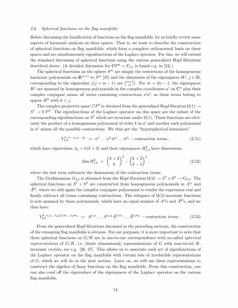
2.6. Spherical functions on the flag manifolds

Before discussing the fuzzification of functions on the flag manifolds, let us briefly review some

aspects of harmonic analysis on these spaces. That is, we want to describe the construction

of spherical functions on flag manifolds, which form a complete orthonormal basis on these

spaces and are simultaneously eigenfunctions of the Laplace operator. For this, we will extend

the standard discussion of spherical functions using the various generalized Hopf fibrations

described above. (A detailed discussion for CPn = F1;n is found e.g. in [24].)

The spherical functions on the sphere Sm are simply the restrictions of the homogeneous

harmonic polynomials on Rm+1 to Sm [25] and the dimension of the eigenspaces Hj, j ∈ N,

corresponding to the eigenvalue j(j + m − 1) are(m+j

m

). For m = 2n − 1, the eigenspaces

Hj are spanned by homogeneous polynomials in the complex coordinates ai on Cn plus their

complex conjugate minus all terms containing contractions aiai, as these terms belong to

spaces Hk with k < j.

The complex projective spaceCP 3 is obtained from the generalized Hopf fibration U(1)→S7 → CP 3. The eigenfunctions of the Laplace operator on this space are the subset of the

corresponding eigenfunctions on S7 which are invariant under U(1). These functions are obvi-

ously the product of a homogeneous polynomial of order k in ai and another such polynomial

in aj minus all the possible contractions. We thus get the “hyperspherical harmonics”

Y k1;4

i1...ikj1...jk := ai1 . . . aik aj1 . . . ajk − contraction terms , (2.51)

which have eigenvalues λk = k(k + 3) and their eigenspaces Hk1;4 have dimensions

dimHk1;4 =

(k + 3

k

)2

−(k + 2

k − 1

)2

, (2.52)

where the last term subtracts the dimensions of the contraction terms.

The Graßmannian G2;4 is obtained from the Hopf fibration U(2)→ S7×S5 → G2;4. The

spherical functions on S7 × S5 are constructed from homogeneous polynomials in Aij and

Akl, where we add again the complex conjugate polynomial to render the expression real and

finally subtract all terms containing contractions. The subspace of U(2)-invariant functions

is now spanned by those polynomials, which have an equal number of Aijs and Akls, and we

thus have:

Y k2;4

i1j1...ikjkl1m1...lkmk := Ai1j1 . . . AikjkAl1m1 . . . Alkmk − contraction terms . (2.53)

From the generalized Hopf fibrations discussed in the preceding sections, the construction

of the remaining flag manifolds is obvious. For our purposes, it is more important to note that

these spherical functions on G/H are in one-to-one correspondence with so-called spherical

representations of G/H, i.e. (finite dimensional) representations of G with non-trivial H-

invariant vectors, see e.g. [26, 27]. This allows us to associate each set of eigenfunctions of

the Laplace operator on the flag manifolds with certain sets of irreducible representations

of G, which we will do in the next section. Later on, we will use these representations to

construct the algebra of fuzzy functions on the flag manifolds. From this construction, one

can also read off the eigenvalues of the eigenspaces of the Laplace operator on the various

flag manifolds.

14

3. Flag manifolds and coherent states

To quantize the flag manifolds, we would like to connect every point on these spaces to a

state in a Hilbert space. A function then automatically becomes an operator on this space.

To establish this connection, recall that every point on a flag manifold which is a coset space

of G = U(n) is in one-to-one correspondence to a generalized coherent state in a specific

representation of G. We will review this relation in the next section and partly follow the

discussion of Perelomov [28], see [29, 15] for quantization using coherent states.

3.1. Representations of SU(n) and coherent states

Consider the Dynkin diagram of SU(n) for simple roots α1, . . . , αn−1

i i . . . ia1 a2 an−1

α1 α2 αn−1(3.1)

An irreducible representation TΛ with highest weight Λ can be labeled by the Dynkin

indices6 a1, . . . , an−1. In the representation (Hilbert) space H Λ, there is a corresponding

highest weight vector |Λ〉 and H Λ has a basis of weight vectors7 |µ〉 i.e. Hj|µ〉 = µj |µ〉.The isotropy subgroup Hµ for any weight vector |µ〉 contains the Cartan subgroup H of

SU(n), which is isomorphic to the maximal torus T n−1 = U(1)×n−1 = U(1)×. . .×U(1) and for

general weight vectors the subgroup Hµ coincides with T n−1. For degenerate representation,

where the highest weight Λ is orthogonal to some simple root αi, i.e.

(Λ, αi) = 0 = ai , (3.2)

the isotropy subgroup Hµ may be larger than T n−1 for some weight vectors. This is evident

since, as explained in appendix B, the ai indicate the highest power of E−α, whose action is

still nontrivial on |Λ〉.A helpful picture arises, when enlarging SU(n) to U(n). The Cartan subalgebra consists

now of n factors of U(1), which one can imagine sitting around the ai. Every ai which is zero

combines the U(m1) left of it with the U(m2) right to it to a U(m1 + m2). This allows us

to construct all the isotropy groups one encounters in flag manifolds, and we will be more

explicit in the next section.

To construct a coherent state system, one has to choose an initial vector |ψ0〉 in H Λ. Then

the system of states |ψg〉 = TΛ(g)|ψ0〉 is called the coherent state system TΛ, |ψ0〉. Let

H0 be the isotropy subgroup for the state |ψ0〉. Then a coherent state |ψg〉 is determined by a

point x = x(g) in the coset space G/H0, corresponding to the element g by |ψg〉 = exp(iα)|x〉up to a phase, |ψ0〉 = |0〉. The isotropy subgroup for a linear combination of weight vectors is,

in general, a subgroup of the Cartan subgroup. Therefore it is convenient to choose a weight

vector |µ〉 as an initial state. For non-degenerate representations, the isotropy subgroup Hµ

is isomorphic to the Cartan subgroup H, and the coherent state |x〉 is characterized by a

point of G/H, or equivalently by a point of the orbit of the adjoint representation

H ′j|x〉 = T (g)HjT

−1(g)|x〉, |x〉 = T (g)|µ〉 . (3.3)

6See appendix B for more details.7which can be chosen to be orthonormal

15

In a representation with some Dynkin labels vanishing, the isotropy subgroup Hµ is larger

than H for some weight vectors |µ〉, in which case the orbit may be degenerate.

There is considerable choice in the selection of the initial state |0〉, even on restriction to

weight vectors. Perelomov [30] has shown that the state |0〉must be |µ〉, where µ is a dominant

weight, if it is to be closest to classical. That is, |µ〉 is obtained from the highest weight by the

Weyl reflection group. Then the coherent states minimize the invariant uncertainty relation

∆C2 = min , (3.4)

where

C2 =∑

j

(Hj)2 +

∑

α∈Σ+

(EαE−α + E−αEα) (3.5)

is the quadratic Casimir operator and

∆C2 = 〈C2〉 −

∑

j

〈Hj〉2 + 2∑

α∈Σ+

〈Eα〉〈E−α〉

. (3.6)

Let us take the initial state to be the highest weight vector |Λ〉. The coherent state system

is then more explicitly defined by

|a〉 = N TΛ(g)|Λ〉 , N−2 = 〈Λ|TΛ(g)|Λ〉 , (3.7)

|a〉 = N exp

∑

α∈Σ+

a−αE−α

exp (hiHi) exp

∑

α∈Σ+

a+αEα

|Λ〉

= N exp

∑

α∈Σ+

a−αE−α

|Λ〉 , (3.8)

where we have restricted ourselves to elements of G which have a Gaußian decomposition.

Note that if some of the Dynkin labels ai vanish (degenerate representations), then the

corresponding coordinates a−α (and possible some others, see the appendix) are no longer

independent and can be eliminated from the definition of the group element g and thus the

coherent states correspond to points on various flag manifolds. The number of independent

coordinates a−α gives the (complex) dimension of the flag manifold.

Note that our construction of coherent states yields merely one patch of the covering of

the flag manifolds. Starting from a different dominant weight state corresponds to working

on a different patch, as the state |w(Λ)〉, where w is an element of the Weyl group W , is

not contained in the set of the coherent states |a〉 constructed from |Λ〉. This is because

we have restricted ourselves to group elements that have a Gaußian decomposition. We can

assume all the weight states to be orthogonal. In particular, two states |Λ〉 and |w(Λ)〉 have

no overlap, i.e. 〈Λ|w(Λ)〉 = 0. Consider now the coherent state |a〉 as constructed above,

|a〉 = N

1 +∞∑

n=1

1

n!

∑

α∈Σ+

a−αE−α

n

|Λ〉 . (3.9)

As E−α contains only lowering operators, we have 〈Λ|E−α|Λ〉 = 0, which implies

〈Λ|a−〉 = 〈Λ|N |Λ〉 + 0 = N . (3.10)

16

It is thus clear that all |a〉 have a component parallel to |Λ〉 and therefore |a〉 never equals

|w(Λ)〉, which we wanted to prove.

The number of such dominant weight states from which we can start and thus the number

of patches is evidently given by the dimension of w(Λ), w ∈W or equivalently the number

of corners of the convex hull of the states in the weight diagram of the representation. This

number is just the rank of the Weyl group modulo group elements acting trivially in a

certain representation. As the Weyl group for SU(n) is essentially the permutation group of

n elements with rank n!, the minimal number of patches covering the complete flag manifold

F123...n−1;n is given by n!, while the number of patches for all other flag manifolds of SU(n)

is smaller. The reason for this is simply that for other flag manifolds, certain Dynkin labels

ai are zero, which implies that the corresponding Weyl reflections

|SαiΛ〉 = |Λ− 2 (αi, Λ)

(αi, αi)αi〉 , (3.11)

act trivially on the highest weight state.

To clarify the above construction, we will first discuss the simple case of flags in SU(3),

whose weight diagrams are two-dimensional, before presenting the construction for the flag

manifolds of SU(4).

3.2. Examples for SU(3)

There are two flag manifolds which arise as coset spaces of SU(3): The complex projective

space CP 2 = F1;3∼= F2;3 = CP 2

∗ ∼= SU(3)U(2) and the reducible flag manifold F12;3 = SU(3)

U(1)×U(1) .

The representations 3, 3 and 6 of SU(3), corresponding to the diagrams

i i1 0

= , i i0 1

= , i i2 0

= , (3.12)

all have dominant weight states with isotropy group U(2). Thus, the coherent states con-

structed from these representations are in one-to-one correspondence with points on CP 2.

The adjoint representation 8 as well as the 27 corresponding to the diagrams

i i1 1

= , i i2 1

= (3.13)

have dominant weight states, whose isotropy group is only the maximal torus U(1) × U(1)

and therefore the derived coherent states are in one-to-one correspondence with points on the

flag manifold F12;3. Recall that the number of patches is found to be the number of corners

in (the convex hulls of) the weight diagrams. Consider e.g. the diagrams

.

. .

.

.

.

.

. .

.

.

.

.

. .

corresponding to the representations with Dynkin labels (1, 0), (1, 1) and (2, 1), respectively.

We see that the complex projective space CP 2 is covered by at least three patches, while the

flag manifold F12;3 requires a minimum of six patches.

17

3.3. The flags in C4

Let us now come to the coherent states which correspond to points on flag manifolds of

SU(4). For these, the choice of representations as well as the Dynkin diagrams are given in

Table 1.

Note that the representations for the reducible flag manifolds are not unique at level L.

One can choose any representation (a1(L), a2(L), a3(L)); however, for considering the limit

L→∞, the functions ai should be polynomials of the same order in L.

The minimal numbers of patches for the various flag manifolds are again the numbers of

corners in the weight diagrams for the various representations. For example, consider the

weight diagrams of the representations (1, 0, 0), (1, 0, 1), (1, 1, 1),

.

..

.

.

.

.

..

.

..

.

.

..

.

.

..

..

.

..

.

..

.

.

.

.

.

.

..

.

...

which yield coherent states corresponding to CP 3, F13;4 and F123;4 with minimal coverings

of 4, 12 and 24 patches, respectively.

dimC patches isotropy group in U(4) Dynkin labels Young diagrams

F1;4 3 4 U(1)× U(3) (L, 0, 0)

L︷ ︸︸ ︷

F2;4 4 6 U(2)× U(2) (0, L, 0)

L︷ ︸︸ ︷

F3;4 3 4 U(3)× U(1) (0, 0, L)

L︷ ︸︸ ︷

F12;4 5 12 U(1)× U(1)× U(2) (L,L, 0)

L+L︷ ︸︸ ︷

F13;4 5 12 U(1)× U(2)× U(1) (L, 0, L)

L+L︷ ︸︸ ︷

F23;4 5 12 U(2)× U(1)× U(1) (0, L, L)

L+L︷ ︸︸ ︷

F123;4 6 24 U(1)× U(1)× U(1)× U(1) (L,L,L)

L+L+L︷ ︸︸ ︷

Table 1: Representations of SU(4) related to the flag manifolds in C4.

18

4. Fuzzification of the flag manifolds

Combining the description of the flag manifolds in terms of Plucker coordinates which we

developed in section 2 with the correspondence to coherent states in the previous section,

we have an obvious way in which one can truncate the algebra of functions on these spaces

to obtain the latter’s fuzzy versions. Before we describe the construction of the fuzzy flag

manifolds in detail, let us briefly recall the underlying principles.

4.1. Fuzzification

By fuzzy geometry, we mean a truncation of the algebra of functions on a compact space such

that the coordinates become noncommutative while all isometries are manifestly preserved.

Given a compact Riemannian manifold M without boundary, the spectrum of the Laplace

operator is discrete and the eigenfunctions form an orthogonal basis B of L2(M). A naıve

guess for a discretization would be to truncate the expansion of a function by using only a

finite subset BL of elements in B. Multiplication of functions, however, clearly necessitates a

subsequent projection back on to BL, which in turn will render the product non-associative

in general.

If the manifold M = G/H is a coadjoint orbit of a Lie group G, we can easily circumvent

this problem: we can map functions to operators acting as automorphisms8 on the represen-

tation space of some representation R of G which admits singlets under H and replace the

product between functions by the operator product. In the previous section, we described

which representations R are suitable for the various flag manifolds of SU(4). We will see that

the choice of R corresponds to a choice of the truncation and the closure of multiplication is

trivially given.

Using a projector ρR(x) = |x〉〈x| which corresponds to a point x ∈ G/H and acts on the

representation space of R, we can establish a map between operators and functions on the

coset space by the formula

fR(x) = tr(ρR(x)f

). (4.1)

The operator product then induces a star product via

(fR ⋆ gR)(x) = tr(ρR(x)f g

). (4.2)

In general, there is an infinite sequence of suitable representations Ri for any coset space and

for each of these representations, the star product is different. Choosing higher-dimensional

representations amounts to a better approximation of the functions by operators, and there

is usually a well-defined limit, in which the complete set of functions on the coset together

with the ordinary product is reproduced.

Let us return to equation (4.1). To each operator f representing a function on MR, assign

a corresponding symbol f(g), g ∈ G by [7]

f(g) = nR tr(DR(g−1)f

), (4.3)

8That is, they can be represented by square matrices.

19

where DR(g) is the group element g acting in the representation R. The normalization

constant nR is defined by∫

dµ(g)DR(g−1)ijDR(g)kl =

1

nRδilδjk (4.4)

with dµ(g) being the Haar measure on G. Inversely, the operator f corresponding to the

symbol f is therefore obtained from

f =

∫dµ(g)f(g)DR(g) . (4.5)

From the symbol f of an operator f , we can easily calculate the function defined in (4.1)

using

fR(x) =

∫dµ(g)ωR(x, g)f (g) with ωR(x, g) := tr

(ρR(x)DR(g)

). (4.6)

In the definition of the star product (4.2), this translates into

(fR ⋆ gR)(x) =

∫dµ(g)

∫dµ(g′)ωR(x, gg′)f(g)g(g′) , (4.7)

and it is for this formula that we will find explicit expressions for all the flag manifolds later

on.

In the discussion of fuzzy flag manifolds using star products, we can use both of the two

equivalent descriptions: either real coordinates describing an embedding of the coset space

into flat Euclidean space or the complex homogeneous or Plucker coordinates. In the latter

coordinates the star product can be shown to simplify considerably. Moreover, they allow

for a direct translation to the operator picture.

Note that so far, we only arrived at an algebra of functions on a topological space. The

explicit geometry of this space, i.e. its metric structure, has not been described yet. In

noncommutative geometry, this information is encoded in a Dirac operator, or – in a slightly

weaker way – in a Laplacian. Using the above mentioned embedding, we obtain a canonical

metric on the coset space and can show that the Laplace operator naturally translates into

the second order Casimir in the representation R.

For more details on the principle underlying fuzzification, see also [5].

4.2. The fuzzy complex projective space CP 3F

The fuzzification of F1;4 (and therefore also that of its dual F3;4) is well-known [5], and we

follow the usual discussion of the procedure for CPN . That is, we promote the vector a and

its complex conjugate a to a four-tuple of annihilation and creation operators satisfying the

algebra [ai, aj†] = δij . The auxiliary coordinates defined in (2.4) also become operators

xa :=1

ak†alδklai†λa

ij aj , (4.8)

which evidently commute with the number operator N = ak†alδkl. Therefore, we can restrict

the algebra of functions to the subspace of the Fock space, on which N = L. This subspace

is spanned by1C a

i1† . . . aiL†|0〉 with C =√n1!n2!n3!n4! , (4.9)

20

where the ni are the number of indices being i. The truncated algebra of functions AL on

this space is the algebra of operators with basis

ai1† · · · aiL†|0〉〈0|aj1 · · · ajL . (4.10)

It is immediately obvious that these operators will commute with the number operator N ,

which amounts to factoring out a U(1) as implied in the definition of any flag manifold. The

coefficients of the expansion of an operator in terms of the basis (4.10) form square matrices

of dimension(

(3+L)!3!L!

)2[5], and in terms of Young diagrams of SU(4), we have

L︷ ︸︸ ︷⊗

L︷ ︸︸ ︷=

L︷ ︸︸ ︷⊗

L︷ ︸︸ ︷. (4.11)

To expose the underlying SU(4) structure and to construct the polarization tensors, we can

contract indices from the creation operators with indices from the annihilation operators using

the 15 generators λaij of SU(4). A contraction with λ0

ij ∼ δij yields the embedded subalgebra

truncated at level L − 1, since the trace over a fundamental and an antifundamental index

corresponds to the determinant over four indices in either the fundamental or antifundamental

representation and thus to a column of 4 boxes in a Young diagram, which is cancelled. The

tensor product expansion looks as

L︷ ︸︸ ︷⊗

L︷ ︸︸ ︷= 1 ⊕ ⊕ ⊕ . . . ⊕

2L︷ ︸︸ ︷. (4.12)

A representation of the Lie algebra of SU(4) is given by the Schwinger construction and

we can write

La = ai†λaij a

j . (4.13)

One can easily verify the algebra [La, Lb] = i√

2fabcL

c using [ai, aj†] = δij .

In the representations R = R(L) introduced above, the projector corresponding in the

case L = 1 to P1;4 = P(x1;4), which describes the embedding of CP 3 in R15, is simply the

L-fold symmetrized tensor product ρL1;4 = ρL(x1;4) = P(x1;4)⊗ . . .⊗P(x1;4), and we can map

any operator f in the algebra AL to a corresponding function fL on the embedding of CP 3

in R15 by

fL(x1;4) = tr (ρL(x1;4)f) . (4.14)

Furthermore, this map induces a star product on CP 3 defined as

(fL ⋆ gL)(x1;4) = fL(x1;4) ⋆ gL(x1;4) = tr (ρL(x1;4)f g) , (4.15)

where fL and gL are the functions corresponding to the operators f and g, respectively.

To make the star product more explicit, we calculate ωL(x1;4, gg′) for the fundamental

representation L = 1:

ωL(x1;4, gg′) = tr (P1;4gg

′) = tr (P1;4gP1;4g′) + tr (P1;4g(1− P1;4)g

′) . (4.16)

Since P1;4 is a rank one projector, we have

tr (P1;4gP1;4g′) = tr (P1;4g) tr (P1;4g

′) = ωL(x1;4, g)ωL(x1;4, g

′) (4.17)

21

and with the identities (2.43), it follows immediately that

tr (P1;4g(1− P1;4)g′) = tr (λag) tr (P1;4λ

a(1− P1;4)g′)

=

(∂

∂xaω(x1;4, g)

)Jab

(∂

∂xbω(x1;4, g

′)

).

(4.18)

For the representations with L > 1, we can simply take the L-fold tensor product of ω1(x1;4, g)

[7]:

ωL(x1;4, g) =(ω1(x1;4, g)

)⊗L, (4.19)

and the total star product reads as [5]

(fL ⋆ gL)(x1;4) =

L∑

l=0

(L− l)!L!l!

(∂a1...alfL(x1;4)) J

a1b11;4 . . . Jalbl

1;4 (∂b1...blgL(x1;4)) . (4.20)

In the homogeneous coordinates ai, ai on CP 3, the space of functions is spanned by homo-

geneous polynomials of the form

ai1 . . . aiLaj1 . . . ajL , (4.21)

which correspond to the operators (4.10) under the map (4.14). In these coordinates, the

star product simplifies to [31]

(f ⋆ g) = µ

[1

L!

∂

∂aα1. . .

∂

∂aαL⊗ 1

L!

∂

∂aα1. . .

∂

∂aαL(f ⊗ g)

], (4.22)

where µ(a⊗ b) = a · b. Note that this construction of a star product generalizes in a rather

straightforward way to other spaces, as soon as we have a suitable projector ρL(x) at hand.

To relate the given matrix algebra to the space CP 3, we need some additional structure

to encode the geometry of this space. For this, consider the vector fields on CP 3 from the

perspective of the embedding space R16:

La = −√

2fabcxb ∂

∂xc, [La,Lb] = i

√2fab

cLc , (4.23)

where fabc are the structure constants of SU(4). Note here that in the limit L → ∞, the

fuzzy derivatives approach the ones from the continuum in an obvious way. It is now rather

straightforward to show that [5]

LafL(x) =√

2Ωab ∂

∂xbfL(x) =

L√2(xa⋆fL(x)−fL(x)⋆xa) = tr

(ρL(x1;4)[L

a, f ]), (4.24)

where [La, ·] are the generators of SU(4) in the representation (L, 0, 0)⊗(0, 0, L). It is therefore

also clear that the Laplace operator on CP 3, ∆ = LaLbδab, is mapped to the second order

Casimir in the adjoint representation (L, 0, 0) ⊗ (0, 0, L):

∆1;4f = [La, [Lb, f ]]δab . (4.25)

22

4.3. The fuzzy Graßmannian GF2;4

We proceed analogously to the case of CP 3, which leads to the results presented in [7] in a

somewhat simpler form. That is, we take the Plucker description discussed in section 2.3.

and promote the vector components to creation and annihilation operators ai, ai†, bi, bi†. We

thus arrive at the algebra

[ai, aj†] = [bi, bj†] = δij , (4.26)

and all other commutators vanish. From these operators, we construct the composite creation

and annihilation operators

Aij2 = a[ibj] and Aij†

2 = a[i†bj]† , (4.27)

which satisfy

[Aij2 , A

kl†2 ] =

(δikδjl + δjlak†ai + δik bl†bj

)

[ij][kl], (4.28)

where (·)[ij][kl] denotes antisymmetrization of the enclosed components, as well as

[[Aij2 , A

kl†2 ], Amn†

2 ] =(2δjlδimAkn†

2

)

[ij][kl][mn]. (4.29)

We can now use Amn†2 to build an L-particle9 Hilbert space H L

2;4. This space is spanned by

1C A

i1j1†2 · · · AiLjL†

2 |0〉 , (4.30)

where C is the norm of the state. Acting with Amn2 on such a state yields a state in H

L−12;4

due to (4.28) and (4.29). Recall that in the Plucker description of G2;4, we constructed the

plane by antisymmetrizing two vectors, which could be chosen orthogonal such that aibi = 0.

On the operator level, this translates into

[ai†bi, Akl†2 ] = 0 , [aibi†, Akl†

2 ] = 0 , [ai†bi, Akl2 ] = 0 and [aibi†, Akl

2 ] = 0 , (4.31)

and therefore the action of ai†bi on any state in H L2;4 vanishes. This implies that we can

introduce the number operator

N = ai†ajδij = bi†bjδij = L (4.32)

and

Aij†2 Akl

2 δikδjl = 2N(N − 1) = 2L(L+ 1) , (4.33)

where the equalities hold only after restriction to H L2;4. Thus, H L

2;4 is indeed an L-particle

Hilbert space. We already know from the discussion in the previous section that the states

(4.30) are invariant under S(U(2)×U(2)). Let us nevertheless be more explicit on the action

of the internal SU(2), which acts nontrivially on both ai and bi. Its generators Lrint act

according to

Lrint = ad

(ai†

p λrpqa

iq

), (4.34)

9Note that a particle is here a composite object consisting of two excitations.

23

where ai1 = ai, ai

2 = bi and λrpq, p, q = 1, 2, r = 1, 2, 3 are the Gell-Mann matrices of SU(2).

The combinations Aij2 and Aij†

2 are now invariant under this action due to the general formula

[ai†p λ

rpqa

iq, a

[j1†1 . . . a

jk]†k ] = 0 , (4.35)

where p = 1, . . . , k and i, jp = 1, . . . , n; see appendix B for a proof.

The truncated algebra of functions AL is the algebra of operators spanned by

Ai1j1†2 · · · AiLjL†|0〉〈0|Ak1 l1 · · · AkLlL

2 , (4.36)

and the coefficients in an expansion in terms of these operators are square matrices of size(3+L)!(2+L)!3!L!2!(L+1)! . Note that these operators again commute with the number operator N and in

terms of Young diagrams, we have here

L︷ ︸︸ ︷⊗

L︷ ︸︸ ︷=

L︷ ︸︸ ︷⊗

L︷ ︸︸ ︷. (4.37)

Again, each of the tensor product decompositions at level L contains the tensor product

decomposition at lower levels:

L︷ ︸︸ ︷⊗

L︷ ︸︸ ︷= 1 ⊕ ⊕ ⊕ ⊕ ⊕ ⊕ . . . (4.38)

Contrary to the case of CP 3, where increasing the level L by one yielded precisely one new

type of Young tableau in the sum, we here obtain L + 1 new diagrams in each step, which

consist of three rows with a + b + a, a + b and a boxes respectively. The new diagrams at

level L are the ones for which a = n and b = 2L− 2n for n = 1 . . . L.

All these notions readily translate for arbitrary Graßmannians.

To find a representation of the Lie algebra of SU(4), we use a generalized Schwinger

construction

La =1

N + 1Aij†

2 ΛaijklA

kl2 with Λa

ijkl = (λa ∧ 1)ijkl . (4.39)

It is important to stress that the La by themselves do not form a representation of SU(4),

but again after having them act on a state in H L2;4, they do. This is simply due to the fact

that because of (4.31), La reduces when acting on a state in H L2;4 to

La = ai†λaij a

j + bi†λaij b

j . (4.40)

The projector yielding a star product on this space is the symmetrized L-fold tensor

product ρL2;4 = ρL(x2;4) = P2;4 ⊗ . . . ⊗P2;4. Proceeding precisely along the lines of the

discussion of the star product on CP 3, we find that

ω1(xab, gg′) = ω1(x, g)(1 +←−∂ abJ

ab,cd−→∂ cd

)ω1(x, g′) , (4.41)

where at least one of the indices in each ab or cd is nonzero. That is, the component x00

plays a similar role to the component x0 in the case of CP 3. Furthermore, one should stress

that as usual for the derivatives on spaces with symmetrized tensors as coordinates, one has

∂ab =

∂

∂xabfor a = b 6= 0

12

∂

∂xabfor a 6= b

. (4.42)

24

It is then quite obvious that the star product is given by

(fL ⋆ gL)(x2;4) =

L∑

l=0

(L− l)!L!l!

(∂(a1 b1)...(al bl)

fL(x2;4))J a1 b1;c1d1

2;4 . . .

J albl;cldl

2;4

(∂(c1d1)...(cldl)

gL(x2;4)),

(4.43)

where ∂(a1 b1)...(al bl):= ∂a1 b1

. . . ∂al bl. Note that our choice of embedding F2;4 in R16·17/2−1

yielded a slightly simpler expression for the star product on this space than the one in [7],

which used an embedding in R15.

The expression for the star product further simplifies, if we switch again to complex

coordinates a[ibj] on C4 ∧C4. The functions corresponding to the operators (4.36) read as

a[i1 bj1] . . . a[iL bjL]a[k1bl1] . . . a[kLblL] (4.44)

and the star product is here defined as

(f ⋆ g) = µ

[1

L!L!

∂

∂a[i1

∂

∂bj1]. . .

∂

∂a[iL

∂

∂bjL]⊗ 1

L!L!

∂

∂a[i1

∂

∂bj1]. . .

∂

∂a[iL

∂

∂bjL](f ⊗ g)

].

The natural Laplacian on H L2;4 encoding the geometry of G2;4 is derived from the embed-

ding of G2;4 in R16·17/2−1. In terms of Plucker coordinates, the generators read as

La = aiλaij∂

∂aj+ biλa

ij∂

∂bj− ajλa

ij∂

∂ai− bjλa

ij∂

∂bi. (4.45)

From this expression and equation (2.9), we obtain the following expression in terms of the

embedding coordinates:

La = −i√

2fabcxbd ∂

∂xcd, (4.46)

which satisfies the algebra [La,Lb] = i√

2fabcLc, as is easily verified. Using the first relation

in (2.47), we can write

LafL(x) =√

2Ia0,cd ∂

∂xcdfL(x) = xa0 ⋆ fL − fL ⋆ x

a0 = −i tr (ρL(x2;4)[La, fL]) . (4.47)

We thus see again that all the derivatives are mapped to the generators of SU(4) acting in the

adjoint and therefore the Laplacian is given by the second order Casimir of this representation

of SU(4),

∆2;4 = adLaadLbδab . (4.48)

This observation from the cases CP 3 and G2;4 translates to all flag manifolds and we suppress

this calculation in the remaining cases. For the discussion of the eigenvalues of these Casimirs,

see appendix B.

4.4. The fuzzy dual complex projective space FF3;4

One can infer the fuzzification of F3;4 in a straightforward manner from the ones of F1;4

and F2;4. We start from the Plucker description and promote the vectors a, b, c to a triple

25

of four-tuples of oscillators with creation and annihilation operators ai, ai†, bi, bi†, ci, ci†. We

furthermore introduce the composite operators

Aijk3 = a[ibj ck] and Aijk†

3 = a[i† bj†ck]† , (4.49)

satisfying the commutation relations

[˜di,

˜d†m] := εijklεmnrs[A

jkl3 , Anrs

3 ]

= δim + εijklεmnrs

(an†ajδrkδsl + δnj br†bkδsl + δnjδrk cs†cl+

an†aj br†bkδsl + an†ajδrk cs†cl + δjnbr†bk cs†cl).

(4.50)

The expression for [[[˜di,

˜d†j ]

˜d†k]

˜d†l ] contains only the combination

˜d†m = εmnrsA

nrs†3 .

The L-particle Fock space H L3;4 is evidently spanned by the states

Ai1j1k1†3 . . . AiLjLkL†

3 |0〉 , (4.51)

and this space forms the representation (0, 0, L) of SU(4). The isotropy subgroup of any state

in this representation is thus S(U(3)×U(1)), and the internal SU(3) action, affecting all the

elementary oscillators a, b, c is given by

Lrint = ad

(ai†

p λrpqa

iq

), (4.52)

where ai1, a

i2, a

i3 stand for ai, bi, ci, respectively, and λr are the Gell-Mann matrices of SU(3).

Invariance of the operators Aijk3 and Aijk†

3 follows from equation (4.35). It is this represen-

tation which underlies the construction of vector bundles over CP 3F [20].

The algebra of functions truncated at level L is again constructed from two copies of the

Fock space and their SU(4) transformation property is captured by the diagrams

L︷ ︸︸ ︷⊗

L︷ ︸︸ ︷=

L︷ ︸︸ ︷ ⊗

L︷ ︸︸ ︷. (4.53)

We clearly see that this algebra is dual to (4.11), i.e. that of FF1;4. For this reason, we will

not go into any further details.

The definition of a star product is obvious. The projector in the symmetrized L-fold

tensor product reads as ρL3;4(x3;4) = P3;4 ⊗ . . .⊗P3;4 and yields

(fL ⋆ gL)(x3;4) =

L∑

l=0

(L− l)!L!l!

(∂(a1 b1c1)...(al blcl)

fL(x3;4))J a1 b1c1;d1e1f1

3;4 . . .

J albl cl;dlelfl

3;4

(∂(d1 e1f1)...(dl elfl)

gL(x3;4)),

(4.54)

where again the components x000 are dropped in the formula and

∂abc =

∂∂xabc for a = b = c 6= 012

∂

∂xabcfor a = b 6= c etc.

16

∂

∂xabcfor a 6= b 6= c 6= a

. (4.55)

26

The discussion of the star product formalism in the complex coordinates a[ibjck] on C4 ∧C4 ∧C4 is trivially deduced from the cases CP 3F and GF

2 . The star product here reads as

(f ⋆ g) = µ[ 1

L!L!L!

∂

∂a[i1

∂

∂bj1∂

∂ck1]. . .

∂

∂a[iL

∂

∂bjL

∂

∂ckL]⊗

⊗ 1

L!L!L!

∂

∂a[i1

∂

∂bj1∂

∂ck1]. . .

∂

∂a[iL

∂

∂bjL

∂

∂ckL](f ⊗ g)

].

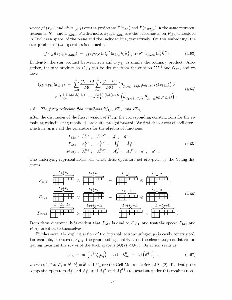
4.5. The fuzzy reducible flag manifold FF12;4

In the case of the reducible flag manifolds, one needs a set of composite creation and annihi-

lation operators. These sets are in one-to-one correspondence with the Plucker coordinates.

For FF12;4 we thus have

Aij2 , Aij†

2 and ai , ai† . (4.56)

The missing commutation relations are easily found from (4.28) and (4.29), e.g.

[ai, Ajk†2 ] = δi[j bk]† (4.57)

and the (L1, L2)-particle Hilbert spaces are now constructed as

Ai1j1†2 . . . A

iL1jL1

†2 ak1† . . . akL2

†|0〉 . (4.58)

The corresponding operators

Ai1j1†2 . . . A

iL1jL1

†2 ak1† . . . akL2

†|0〉〈0|Am1n1

2 . . . AmL1

nL1

2 al1 . . . alL2 (4.59)

evidently form a closed algebra and act on the representation space of the representation

given in terms of Young diagrams by

L1+L2︷ ︸︸ ︷⊗

L1+L2︷ ︸︸ ︷=

L2+L1︷ ︸︸ ︷⊗

L1+L2︷ ︸︸ ︷(4.60)

The internal isotropy subgroup here is U(1)×U(1), which follows from the discussion of the

underlying coherent states. The explicit action of this subgroup on the elementary oscillators

is given by the number operators for ai and bi.

Note that the full algebra of functions on the flag manifold is obtained from the Hilbert

space, which is the sum of all representations with L1 + L2 = L for some fixed L. This is

somewhat evident as the algebra of functions on FF12;4 should contain both the algebra of

functions of FF1;4 and FF

2;4 at level L.

To define a star product on this space, recall that we could describe the flag manifold

F12;4 in terms of two rank one projectors P2 and P1 satisfying P2P1P2 = P1. Furthermore,

note that we can split every operator f in this representation as

f = fIJ hI2 ⊗ hJ

1 with hI2 ∈

L1︷ ︸︸ ︷⊗

L1︷ ︸︸ ︷and hJ

1 ∈

L2︷ ︸︸ ︷⊗

L2︷ ︸︸ ︷, (4.61)

where I and J are multi-indices. To such an operator, a truncated function is assigned by

f(x2;4, x1(2);4) = fIJ tr (ρL(x2;4)hI2) tr (ρL(x1(2);4)h

J1 ) , (4.62)

27

where ρL(x2;4) and ρL(x1(2);4) are the projectors P(x2;4) and P(x1(2);4) in the same represen-

tations as hI1,2 and x1(2);4. Furthermore, x2;4, x1(2);4 are the coordinates on F12;4 embedded

in Euclidean space, of the plane and the included line, respectively. On this embedding, the

star product of two operators is defined as

(f ⋆ g)(x2;4, x1(2);4) = fIJ gMN tr (ρL(x2;4)hI2h

M2 ) tr (ρL(x1(2);4)h

J1 h

N1 ) . (4.63)

Evidently, the star product between x2;4 and x1(2);4 is simply the ordinary product. Alto-

gether, the star product on F12;4 can be derived from the ones on CP 3 and G2;4, and we

have

(fL ⋆ gL)(x12;4) =L∑

l=0

(L− l)!L!l!

L∑

k=0

(L− k)!L!k!

(∂(a1 b1)...(al bl)

∂e1...ekfL(x12;4)

)×

× J (a1 b1),(c1d1);e1f1

12;4 . . . J(al bl),(cldl);ekfk

12;4

(∂(c1d1)...(cldl)

∂f1...fkgL(x12;4)

).

(4.64)

4.6. The fuzzy reducible flag manifolds FF23;4, F

F13;4 and FF

123;4

After the discussion of the fuzzy version of F12;4, the corresponding constructions for the re-

maining reducible flag manifolds are quite straightforward. We first choose sets of oscillators,

which in turn yield the generators for the algebra of functions:

F13;4 : Aijk3 , Aijk†

3 , ai , ai† ,

F23;4 : Aijk3 , Aijk†

3 , Aij2 , Aij†

2 ,

F123;4 : Aijk3 , Aijk†

3 , Aij2 , Aij†

2 , ai , ai† .

(4.65)

The underlying representations, on which these operators act are given by the Young dia-

grams

F13;4 :

L1+L2︷ ︸︸ ︷⊗

L1+L2︷ ︸︸ ︷=

L2+L1︷ ︸︸ ︷⊗

L1+L2︷ ︸︸ ︷,

F23;4 :

L1+L2︷ ︸︸ ︷⊗

L1+L2︷ ︸︸ ︷=

L2+L1︷ ︸︸ ︷⊗

L1+L2︷ ︸︸ ︷,

F123;4 :

L1+L2+L3︷ ︸︸ ︷⊗

L1+L2+L3︷ ︸︸ ︷=

L3+L2+L1︷ ︸︸ ︷⊗

L1+L2+L3︷ ︸︸ ︷.

(4.66)

From these diagrams, it is evident that F23;4 is dual to F12;4, and that the spaces F13;4 and

F123;4 are dual to themselves.

Furthermore, the explicit action of the internal isotropy subgroups is easily constructed.

For example, in the case F23;4, the group acting nontrivial on the elementary oscillators but

leaving invariant the states of the Fock space is SU(2)× U(1). Its action reads as

Lrint = ad

(ai†

p λrpqa

iq

)and L0

int = ad(ci†ci

), (4.67)

where as before ai1 = ai, ai

2 = bi and λrpq are the Gell-Mann matrices of SU(2). Evidently, the

composite operators Aij2 and Aij†

2 and Aijk3 and Aijk†

3 are invariant under this combination.

28

The definition of a star product is performed analogously to the case of F12;4. We de-

compose an operator f representing a function on a fuzzy flag manifold into

f = fIJ hIk1⊗ hJ

k2and f = fIJKh

I3 ⊗ hJ

2 ⊗ hJ1 (4.68)

for Fk1k2;4 and F123;4, respectively. The map from operators to functions reads as

f(xk2;4, xk1(k2);4) = fIJ tr (ρL1(xk2;4)hIk2

) tr (ρL2(xk1(k2);4)hJk1

) (4.69)

and

f(x3;4, x2(3);4, x1(23);4) = fIJK tr (ρL1(x3;4)hI3) tr (ρL2(x2(3);4)h

J2 ) tr (ρL3(x1(23);4)h

J1 ) ,

(4.70)

which naturally induces a star product via the usual formula. The explicit form of the star

products are then obtained from the obvious sums over the differential operators

F13;4 :←−∂ (a1 b1c1)...(al blcl)

←−∂ g1...gk

J(a1 b1c1),(d1e1f1);g1h1

13;4 . . .

J(al bl cl),(dl elfl);gkhk

13;4

−→∂ (d1e1f1)...(dl elfl)

−→∂ h1...hk

,

F23;4 :←−∂ (a1 b1c1)...(al blcl)

←−∂ (g1h1)...(gkhk)J

(a1 b1c1),(d1 e1f1);(g1h1),(m1n1)23;4 . . .

J(al bl cl),(dl elfl);(gkhk),(mknk)23;4

−→∂ (d1e1f1)...(dl elfl)

−→∂ (m1n1)...(mknk) ,

F123;4 :←−∂ (a1 b1c1)...(al blcl)

←−∂ (g1h1)...(gkhk)

←−∂ p1...pr

J(a1 b1c1),(d1 e1f1);(g1h1),(m1n1);p1q1

123;4 . . .

J(al bl cl),(dl elfl);(gkhk),(mknk);pr qr

123;4

−→∂ (d1e1f1)...(dl elfl)

−→∂ (m1n1)...(mknk)

−→∂ q1...qr

.

4.7. Continuous limits of the fuzzy flag manifolds

As a consistency check, one can calculate the dimension of the continuous flag manifolds from

considering the L→∞ limit of the various representations used in describing the fuzzy alge-

bra of functions on them. The underlying idea is simply that given a cutoff L, the number of

eigenvalues should be proportional to Ld on a d-dimensional manifold. The number of degrees

of freedom in the matrix algebras was the square of the dimension d(a1(L), a2(L), a3(L)) of

the representation (a1(L), a2(L), a3(L)), and we can thus deduce that

d = limL→∞

ln(d(a1(L), a2(L), a3(L)))

lnL. (4.71)

A trivial calculation shows that the representations and the matrix algebras we have chosen

in the previous sections indeed reproduce the right dimensions for the various flag manifolds:

Flag manifold F1;4 F2;4 F3;4 F12;4 F13;4 F23;4 F123;4

representations (L, 0, 0) (0, L, 0) (0, 0, L) (L,L, 0) (L, 0, L) (0, L, L) (L,L,L)

real dimension 6 8 6 10 10 10 12

Considering the expressions for the star products on the various flag manifolds found in

the previous sections, it is also evident that the star or operator product will go over to the

commutative product in the limit L → ∞. As discussed in [31], this limit is, however, not

clearly observable in the simplified formulæ using the complex coordinates ai, bi, ci. Further-

more, the derivatives in the fuzzy case containing the geometric information are evidently

approaching the derivatives in the continuum for L→∞.

29

5. Super Plucker embeddings and flag supermanifolds

5.1. Flag supermanifolds of U(4|n)

Flag supermanifolds can be defined analogously to bosonic flag manifolds by considering the

supervector space Cm|n [18]; see also appendix A for more details. A superflag is a sequence

of superspaces VD1( . . . ( VDk

⊂ Cm|n such that dimC VD = D = d|δ. Note that inclusion

requires that di ≤ dj and δi ≤ δj for i < j with at least one inequality being strict. A flag

supermanifold FD1...Dk;m|n is correspondingly the set of all superflags fD1...Dk;m|n. One can

again write a flag supermanifold as a coset space:

FD1...Dk;m|n = U(m|n)/(U(m− dk|n− δk)× . . .× U(d1|δ1)) . (5.1)

The special unitary supergroups SU(m|n) are not useful here, as for m = n, one has to

exclude the identity matrix, which is a central element in this case, from the set of generators

of su(m|n). See appendix A for more details on this point.

As before, we will be interested in the flag manifolds arising naturally in the double

fibration underlying well-known supertwistor correspondences. These spaces are flags in the

superspace C4|n, and because there are again natural projections, they fit into the following

diagram:

F(1|0);(4|n)

F(1|0)(2|0)(2|n)(3|n);(4|n)

F(2|0)(2|n)(3|n);(4|n)

F(2|0)(2|n);(4|n)

F(1|0)(2|0)(2|n);(4|n)

F(3|n);(4|n)

F(1|0)(3|n);(4|n)

6

?

:XXXXy

XXXXz9

6 6:XXXXy

XXXXz

9XXXXz

9XXXXz

(5.2)

Here, F(1|0);(4|n) is the superspace CP 3|n and F(2|0)(2|n);(4|n) is the conformal compactifica-

tion of super Minkowski space with n = N being the number of supersymmetries. Note

that F(2|0)(2|n);(4|n) contains the left chiral superspace F(2|0);(4|n) as well as the right chiral

superspace F(2|n);(4|n) [18]. Since in the twistor correspondences involving F(1|0);(4|n) and

F(3|n);(4|n), only these chiral subspaces play a role, we will also restrict the correspondence

spaces and only consider F(1|0)(2|0);(4|n) and F(2|n)(3|n);(4|n) instead of F(1|0)(2|0)(2|n);(4|n) and

F(2|0)(2|n)(3|n);(4|n).

To get a reliable handle on the geometry of the flag supermanifolds, it is useful to introduce

local coordinates. For simplicity, we will first consider the ordinary Graßmannians and then

discuss the super case. The extension to reducible flag supermanifolds will be straightforward.

On a Graßmannian Gk;n, a patch corresponds to a subset I ⊂ 1, . . . , n with k elements,

which selects k columns of a k×n matrix Z. We identify these columns with the columns of a

k× k unit matrix; they fix parts of the vectors spanning the k-dimensional vector subspaces.

The remaining columns are filled by the local coordinates on the patch I. As an example,

consider CP 2 = G1;3, where there are three patches

Z1 = (1 z11 z

21) , Z2 = (z1

2 1 z22) and Z3 = (z1

3 z23 1) . (5.3)

Transition functions are elements of a finite subgroup of GL(n,C), permuting the k× k unit

30

matrix to different columns. We also see that on every patch we have the U(k)×U(n− k) ⊂U(n) invariance manifest.

For a super GraßmannianGk|κ;n|ν, we consider a (k|κ)×(k+(n−k)|κ+(ν−κ))-dimensional

supermatrix ZI , into which we insert the columns of the k|κ× k|κ-dimensional unit matrix,

preserving the grading of the matrix. The set I of the columns which we selected corresponds

again to a patch. The discussion of the transition functions is the same as in the bosonic

case and the symmetries factored out are again manifest.

A first observation is that for the super Graßmannians we are interested in, the fermionic

dimension of the subspace is always either maximal or minimal. This leads e.g. to matrices

ZI

G2|0;4|4 : Z34|· =(x2×2 12×2 ξ2×4

),

G2|0;2|4 : Z12|· =( 12×2 ξ2×4

),

G2|4;4|4 : Z34|1234 =

(x2×2 12×2 02×4

ξ4×2 04×2 14×4

),

(5.4)

where the lines indicate the boundaries of the four canonical blocks in the supermatrix

Z. The first and the third space are the compactified, complexified chiral and anti-chiral

N = 4 superspaces, respectively. It is easy to convince oneself that (the bosonic part of)

the transition functions are the same as in the purely bosonic case. Therefore, the super

Graßmannian (and also the flag supermanifolds) we are dealing with are simply certain

fermionic vector bundles over their bodies, i.e. the embedded ordinary flag manifolds. As an

explicit example, consider the space CP 1|2. Following our discussion of local coordinates, we

introduce the two patches U±, corresponding to the matrices

Z+ = (z+ 1 ζ1+ ζ2

+) and Z− = (1 z− ζ1− ζ2

−) . (5.5)

The transition function between both patches is evidently f+− = z+ and therefore we have

ζ1,2+ = z+ζ

1,2− . Thus, the space CP 1|2 is the total space of the rank 0|2 vector bundle

ΠO(1)⊕ΠO(1) → CP 1 . (5.6)

For more details on the definition of super Graßmannians and flag supermanifolds, see [32].

For simplicity, we restrict our attention to the case n = N = 4 in the following. Using

the description of super Graßmannians given above, it is easy to determine the dimensions

of the various flag supermanifolds in (5.2) for n = 4. We have

F(1|0);(4|4) : 3|4 F(2|0);(4|4) : 4|8F(2|4);(4|4) : 4|8 F(2|0)(2|4);(4|4) : 4|16

F(1|0)(2|0);(4|4) : 5|8 F(3|4);(4|4) : 3|4F(2|4)(3|4);(4|4) : 5|8 F(1|0)(3|4);(4|4) : 5|16

F(1|0)(2|0)(2|4)(3|4);(4|4) : 6|16 .

(5.7)

The minimal numbers of patches covering the flag supermanifolds are the same as the ones

for their bodies.

31

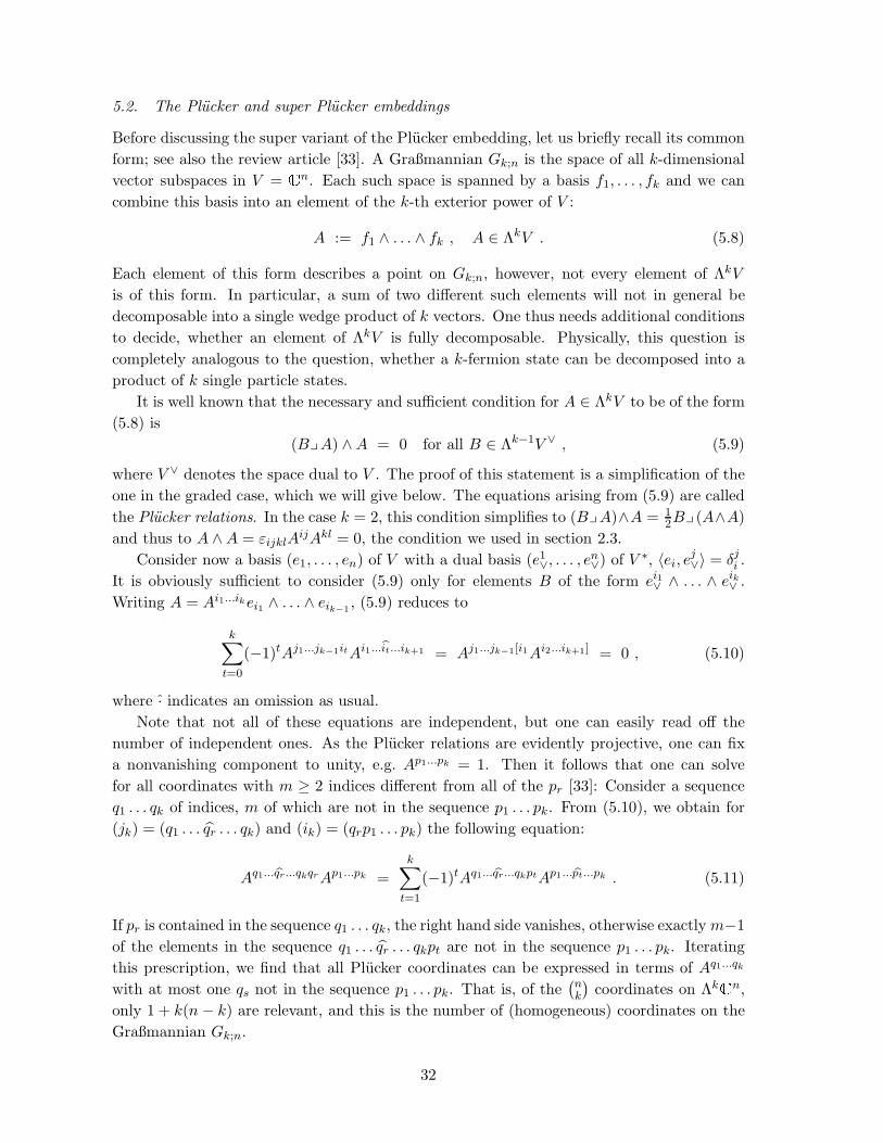
5.2. The Plucker and super Plucker embeddings

Before discussing the super variant of the Plucker embedding, let us briefly recall its common

form; see also the review article [33]. A Graßmannian Gk;n is the space of all k-dimensional

vector subspaces in V = Cn. Each such space is spanned by a basis f1, . . . , fk and we can

combine this basis into an element of the k-th exterior power of V :

A := f1 ∧ . . . ∧ fk , A ∈ ΛkV . (5.8)

Each element of this form describes a point on Gk;n, however, not every element of ΛkV

is of this form. In particular, a sum of two different such elements will not in general be

decomposable into a single wedge product of k vectors. One thus needs additional conditions

to decide, whether an element of ΛkV is fully decomposable. Physically, this question is

completely analogous to the question, whether a k-fermion state can be decomposed into a

product of k single particle states.

It is well known that the necessary and sufficient condition for A ∈ ΛkV to be of the form

(5.8) is

(ByA) ∧A = 0 for all B ∈ Λk−1V ∨ , (5.9)

where V ∨ denotes the space dual to V . The proof of this statement is a simplification of the

one in the graded case, which we will give below. The equations arising from (5.9) are called

the Plucker relations. In the case k = 2, this condition simplifies to (ByA)∧A = 12By (A∧A)

and thus to A ∧A = εijklAijAkl = 0, the condition we used in section 2.3.

Consider now a basis (e1, . . . , en) of V with a dual basis (e1∨, . . . , en∨) of V ∗, 〈ei, ej∨〉 = δj

i .

It is obviously sufficient to consider (5.9) only for elements B of the form ei1∨ ∧ . . . ∧ eik∨ .

Writing A = Ai1...ikei1 ∧ . . . ∧ eik−1, (5.9) reduces to

k∑

t=0

(−1)tAj1...jk−1itAi1...bit...ik+1 = Aj1...jk−1[i1Ai2...ik+1] = 0 , (5.10)

where · indicates an omission as usual.

Note that not all of these equations are independent, but one can easily read off the

number of independent ones. As the Plucker relations are evidently projective, one can fix

a nonvanishing component to unity, e.g. Ap1...pk = 1. Then it follows that one can solve

for all coordinates with m ≥ 2 indices different from all of the pr [33]: Consider a sequence

q1 . . . qk of indices, m of which are not in the sequence p1 . . . pk. From (5.10), we obtain for

(jk) = (q1 . . . qr . . . qk) and (ik) = (qrp1 . . . pk) the following equation:

Aq1... bqr...qkqrAp1...pk =

k∑

t=1

(−1)tAq1... bqr...qkptAp1... bpt...pk . (5.11)

If pr is contained in the sequence q1 . . . qk, the right hand side vanishes, otherwise exactly m−1

of the elements in the sequence q1 . . . qr . . . qkpt are not in the sequence p1 . . . pk. Iterating

this prescription, we find that all Plucker coordinates can be expressed in terms of Aq1...qk

with at most one qs not in the sequence p1 . . . pk. That is, of the(nk

)coordinates on ΛkCn,

only 1 + k(n − k) are relevant, and this is the number of (homogeneous) coordinates on the

Graßmannian Gk;n.

32

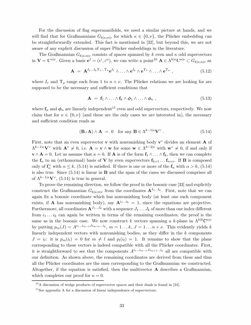
For the discussion of flag supermanifolds, we need a similar picture at hands, and we

will find that for Graßmannians Gk|κ;n|ν for which κ ∈ 0, ν, the Plucker embedding can

be straightforwardly extended. This fact is mentioned in [32], but beyond this, we are not

aware of any explicit discussion of super Plucker embeddings in the literature.

The Graßmannian Gk|κ;n|ν consists of spaces spanned by k even and κ odd supervectors

in V = Cn|ν. Given a basis eI = (ei, εα), we can write a point10 A ∈ Λk|κCn|ν ⊂ Gk|κ;n|ν as

A = AI1...IkΥ1...ΥκeI1 ∧ . . . ∧ eIk ∧ eΥ1 ∧ . . . ∧ eΥκ , (5.12)

where Ir and Υρ range each from 1 to n + ν. The Plucker relations we are looking for are

supposed to be the necessary and sufficient conditions that

A = f1 ∧ . . . ∧ fk ∧ φ1 ∧ . . . ∧φκ , (5.13)

where fα and φα are linearly independent11 even and odd supervectors, respectively. We now

claim that for κ ∈ 0, ν (and these are the only cases we are interested in), the necessary

and sufficient condition reads as

(ByA) ∧A = 0 for any B ∈ Λk−1|κV∨ . (5.14)

First, note that an even supervector v with nonvanishing body v divides an element A of

Λk−1|κV∨ with A 6= 0, i.e. A = v ∧ w for some w ∈ Λk−2|κ with w 6= 0, if and only if

v ∧A = 0. Let us assume that κ = 0. If A is of the form f1 ∧ . . . ∧ fk, then we can complete

the fα to an (orthonormal) basis of V by even supervectors fk+1 . . . fn+ν . If B is composed

only of f∨α with α ≤ k, (5.14) is satisfied. If there is one or more of the fα with α > k, (5.14)

is also true. Since (5.14) is linear in B and the span of the cases we discussed comprises all

of Λk−1|κV∨, (5.14) is true in general.

To prove the remaining direction, we follow the proof in the bosonic case [33] and explicitly

construct the Graßmannian Gk|κ;n|ν from the coordinates AI1...Ik . First, note that we can

again fix a bosonic coordinate which has nonvanishing body (at least one such component

exists, if A has nonvanishing body), say Ai1...ik = 1, since the equations are projective.

Furthermore, all coordinates AJ1...Jk with a sequence J1 . . . Jk of more than one index different

from i1 . . . ik can again be written in terms of the remaining coordinates; the proof is the

same as in the bosonic case. We now construct k vectors spanning a k-plane in Λk|0Cn|ν

by putting pm(J) = Ai1...im−1Jim+1...ik , m = 1 . . . k, J = 1 . . . n + ν. This evidently yields k

linearly independent vectors with nonvanishing bodies, as they differ in the k components

J = il: it is pm(il) = 0 for m 6= l and pl(il) = 1. It remains to show that the plane

corresponding to these vectors is indeed compatible with all the Plucker coordinates. First,

it is straightforward to see that the components Ai1...im−1Jim+1...ik all are compatible with

our definition. As shown above, the remaining coordinates are derived from these and thus

all the Plucker coordinates are the ones corresponding to the Graßmannian we constructed.

Altogether, if the equation is satisfied, then the multivector A describes a Graßmannian,

which completes our proof for κ = 0.

10A discussion of wedge products of supervector spaces and their duals is found in [34].11See appendix A for a discussion of linear independence of supervectors.

33

For κ = ν, it is sufficient to note that the wedge product of the ν odd supervectors in A

either vanishes, if they are linearly dependent, or spans all of the odd supspace. Therefore,

it suffices again to focus on the even supervectors in A, which is done by contracting with a

dual multivector B ∈ Λk−1|νV∨, and there is nothing left to prove.

5.3. Plucker coordinates and projector description of irreducible flag supermanifolds

From the discussion in section 5.1., the description of CP 3|4 is evident: homogeneous coor-

dinates on CP 3|4 are provided by the components of an even supervector (normalized and in

a representation of type I, i.e. in a pure even basis) aI = (ai, ηα). From the discussion above,

we know that the space CP 3|4 is the fermionic rank 4 vector bundleC4 ⊗ΠO(1) → CP 3 , (5.15)

and its sections are given by homogeneous polynomials of degree one in the coordinates onCP 3. We can therefore rewrite the fermionic components of the even supervector aI as

ηα = ηαi a

i with ηαi ∈ C0|8 . (5.16)

In the following, however, we will not be interested in sections of this bundle but rather in

the algebra of functions on its total space.

We therefore continue along the lines of the bosonic case and construct a projector using

the supervector a according to

P1|0 = aaT . (5.17)

Note that the description of a flag manifold using projectors trivially generalizes to the

supercase. First of all, the bodies of even and odd supervectors of dimension 4|4 have non-

zero components in the first and the last four components, respectively. This property is

preserved by the action of U(4|4). Thus, given a projector

P =

(PA PB

PC PD

), (5.18)

we can read off the dimension k|κ of the subspace of C4|4 onto which it projects to be

tr (PA)| tr (P

D), where · denotes the body of the projector. We will define the rank of such

a projector to be k|κ.Also, there is a subgroup U(4− k|4 − κ) of U(4|4), which leaves invariant a projector of

rank k|κ. This is easily seen by the usual identification of u(4|4) with u(4+4) after combining

the odd generators with an odd parameter and the fact that the rank of a projector is left

invariant by the action of U(4|4).For P1|0 to be a projector, we have to demand that

(a,a) = aa = aiai + iηαηα = 1 , (5.19)

see appendix A for a definition of the scalar product of complex supervectors. This condition

can also be understood from the construction of CPn|n+1 viaCn+1|n+1 → S2n+1|2n+2 → CPn|n+1 , (5.20)

34

as the first projection, see also [35]. We can in fact introduce coordinates xA = aIλAIJa

J in the

superspace R32|32, where the λA are the generators of U(4|4) as described in the appendix.

The coordinates xA describe an embedding of CP 3|4 in R32|32 and due to λAIJλB

KLgAB =

δILδJK , we have

P1|0 = xAλBgAB = aaT . (5.21)

Underlying this construction is again a generalized Hopf fibration

1 −→ U(1) −→ S2n+1|2n+2 −→ CPn|n+1 −→ 1 . (5.22)

Let us now turn to the Graßmannians, whose description is rather straightforward using

the super Plucker embedding. We start with G2|0;4|4, and the Plucker coordinates are given

by

A[IJ ]2|0 = a[IbJ ] = aIbJ − (−1)I JaJbI = aIbJ − bIaJ , (5.23)

where a = (a, η) and b = (b, ζ) are two even supervectors, [·, ·] is the supercommutator and

I denotes the parity of the corresponding index. That is, i = 0 and α = 1, plus the parity of

the supervector under consideration, modulo 2. In more detail, we have

Aij2|0 = a[ibj] , Aiα

2|0 = −Aαi2|0 = 1

2

(aiζα − ηαbi

)and A

αβ2|0 = ηαζβ , (5.24)

where · denotes symmetrization, in particular of Graßmann-odd quantities. Note that this

super-antisymmetrized combination of a and b indeed eliminates all components of b parallel

to a and in the following, we will assume that b and a are perpendicular:

aIbI = aibi + iζαηα = 0 . (5.25)

Together with a 6= 0 6= b, this equation implies that both supervectors are linearly inde-

pendent. The (internal) stabilizer subgroup of U(4|4) leaving AIJ2|0 invariant is U(2|0), which

rotates the supervector a into b and vice versa; see the discussion of the fuzzy case for more

details.

We observed before that the Plucker coordinates Aij2 on G2;4 contain some redundancy:

first there is a scaling, which renders them effectively coordinates on CP 5, and second, there

is the identity εijklAij2 A

kl2 = 0. In the present case, the redundancy is somewhat larger, but

from the discussion of the super Plucker embedding, we can be specific about the number of

redundant coordinates. First of all, we have 16 even and 16 odd homogeneous coordinates

and thus we are using a Plucker embedding into CP 15|16. Assuming that A122|0 = 1 fixes the

scaling, only the coordinates

A132|0 A14

2|0 A152|0 . . . A18

2|0A23

2|0 A242|0 A25

2|0 . . . A282|0

(5.26)

are independent and we thus arrive at a 4|8-dimensional space, G2|0;4|4.From the bi-supervector A2|0, one can again construct a projector:

(P2|0;4|4)IJ ;KL = AIJ

2|0AKL2|0 (5.27)

35

and with our choice and the orthonormality of a and b, P2|0;4|4 satisfies indeed (P2|0;4|4)2 =

P2|0;4|4. Underlying the construction of this projector is again a generalized Hopf fibration,

which is evidently a superextension of the one for G2;4:

1 −→ U(2|0) −→ S7|8 × S5|8 −→ F2|0;4|4 −→ 1 . (5.28)

It is now necessary to introduce a super-antisymmetrized tensor product defined as

(A ⋓ B)IJ ;KL := 14

(AIKBJL − (−1)I JAJKBIL−

(−1)KLAILBJK + (−1)I J(−1)KLAJLBIK

).

(5.29)

As in the case of the antisymmetric product of the generators of U(4), we also have here

various Fierz identities, see appendix A. Using one of these identities, we can introduce the

projector

(P2|0;4|4)IJ ;KL = AKL2|0 AIJ

2|0

= AK ′L′

2|0 (λA⋓ λB)K ′L′I′J ′AI′J ′

2|0 (λC⋓ λD)IJ ;KL gAC gBD

=: xAB(λC⋓ λD)IJ ;KL gAC gBD .

(5.30)

The next Graßmannian to be described is the space G2|4;4|4. This space is certainly

“dual” to G2|0;4|4, as one easily guesses from the description in terms of coordinate matrices

ZI given in the previous section. To describe this space, one needs to take two even and

four odd normalized supervectors and then super-antisymmetrize them. A short remark is

in order to show that super-antisymmetrizing indeed yields a projection on their mutually

orthogonal components. We saw above that this is true for two even supervectors. Since

the bodies of normalized even and odd supervectors are non-vanishing exactly in the even

and odd indices, respectively, a pair of an even and an odd normalized supervector are

always linearly independent; antisupersymmetrization just eliminates redundancies in the

description of 1|1-dimensional subspaces via Plucker relations. Given two odd supervectors,

super-antisymmetrization has the same effect on the even and odd components as it had on

two even supervectors and thus projects out non-orthogonal components.

Altogether, we have Plucker coordinates

AIJΥ1...Υ4

2|4 = a[IbJηΥ1 . . .ηΥ4] , (5.31)

where aI ,bI and ηΥ are even and odd supervectors, respectively. We assume that A12456782|4 =

1 to fix the scale. From the discussion of the super Plucker embedding, it then follows that

the independent coordinates here are given by

A1356782|4 A145678

2|4 A1556782|4 . . . A185678

2|4A235678

2|4 A2456782|4 A255678

2|4 . . . A2856782|4

. (5.32)

In the case of the dual complex projective superspace CP 3|4∗ , we add to this picture

another even supervector cI and obtain the Plucker coordinates

AIJKΥ1...Υ4

2|4 = a[IbJcKηΥ1 . . .ηΥ4] , (5.33)

36

where aI ,bI and ηΥ are even and odd supervectors, respectively. We fix the scale by

A123456783|4 = 1 and the remaining independent coordinates here are

A12456783|4 A1345678

3|4 A23456783|4 A155678

3|4 . . . A1856782|4 . (5.34)

We refrain from going into any further detail at this point and refer to the discussion of the

fuzzy pictures of these super Graßmannians.

5.4. The reducible flag supermanifolds

As in the bosonic case, the description of the reducible flag supermanifolds is merely a

combination of the underlying “elementary” Graßmannians.

The complexified, compactified super Minkowski space F(2|0)(2|4);(4|4) is a reducible flag su-

permanifold, although its body is an irreducible flag manifold. Combining the sets of Plucker

coordinates on G2|0;4|4 and G2|4;4|4 and factoring out redundancies arising from the fact that

the even supervectors in both cases are the same, one arrives at the Plucker coordinates on

the space F(2|0)(2|4);4|4, which is of superdimension 4|16.Similarly, the remaining flag supermanifolds are constructed by combining the coordinates

of the Graßmannians corresponding to the various subflags. Again, a more detailed discussion

will be presented, when we develop the fuzzy versions of these spaces.

5.5. Geometric structures on the flag supermanifolds

The description of the flag supermanifolds in terms of projectors allows us to proceed similarly

to the case of ordinary flag manifolds in the description of their geometry. That is, we describe

a point on a flag supermanifold M again by a projector P0, and the action of G = U(4|4)on this point produces all of M. The coordinates xA provide an embedding of M in Rm|n

(e.g. CP 3|4 is embedded in R32|32). The tangent vectors at P0 are naturally obtained from

an appropriate action R(Λ) on P0 and we define analogously to the bosonic case

TP0M = R(Λ)P0|Λ ∈ u(4|4) . (5.35)

The generators of the subgroup H in M = G/H will leave P0 invariant, and thus TP0M is of

the same dimension as M. In the case of CP 3|4, R(Λ) is the superadjoint action, and since

P0 is an even supermatrix, it is thus clear that a vector V ∈ TP0M satisfies

P0,V = V and strV = 0 . (5.36)

From this point, it is rather obvious that we can proceed with the definition of the complex

structure, the metric, as well as the Kahler structure exactly as in the bosonic case. We

thus go over to an arbitrary projector P describing any point on M and define the complex

structure as

IV := −i[P,V] = −i[P,V] , (5.37)

which trivially satisfies I2 = −1 and the hermitian supermetric as

g(V1,V2) = − str (IV1IV2) , (5.38)

37

which satisfies g(IV1, IV2) = g(V1,V2), is invariant under the action of U(4|4) on the vectors

V1 and V2 and defines a supersymmetric even tensor: g(V1,V2) = (−1)V1V2g(V2,V1).

Evidently, there is the supersymplectic structure

Ω(V1,V2) = g(IV1,V2) , (5.39)

satisfying Ω(V1,V2) = −(−1)V1V2Ω(V2,V1), from which we obtain the super Kahler struc-

ture J as

J(V1,V2) = 12(g(V1,V2) + iΩ(V1,V2)) = str (PV1(1− P)V2) . (5.40)

Note that for any normalized supervector a, there is a transformation g ∈ U(4|4) map-

ping it to the vector a′ = (1, 0, . . .)T . This implies that by an appropriate action of g,

one can turn P into diag(1, 0, . . .) and therefore we have again the formula str (PAPB) =

str (PA) str (PB) , which allows us to write

J(V1,V2) = str (PV1V2)− str (PV1) str (PV2) . (5.41)

Furthermore, we introduce the obvious components JAB = J(λA,λB) etc., for which we have

e.g. the identity

JABλB = str (PλA(1− P)λB)λB = PλA(1− P) . (5.42)

Note that a projection onto the body of all the structures introduced in this section

naturally reduces them to their ordinary counterparts on bosonic flag manifolds. These

geometric structures are thus (unique) supersymmetric extensions. Furthermore, the above

discussion naturally extends to the case of all other flag supermanifolds involving super-

antisymmetrized tensor products of the type λA⋓ λB

⋓ . . ..

6. Fuzzy flag supermanifolds

Having a description of flag supermanifolds using the Plucker embedding, we obtain quite

straightforwardly the description of fuzzy flag supermanifolds. We will be rather concise and

essentially stress the differences with the bosonic case. For earlier accounts of quantizingCP 1|2, see e.g. [36].

6.1. Supercoherent states

The discussion of supercoherent states is done in close analogy to the case of bosonic coherent

states. Consider the generators of the supergroup U(4|4). After taking out the matrix

diag(14,−14), we are left with 31 bosonic and 32 fermionic generators. There are seven

generators of the Cartan subalgebra: the six Cartan generators of the two SU(4)s contained

in U(4|4) together with 18. We pair the remaining 24 bosonic and 30 fermionic generators

into raising and lowering operators. Seven of them are fundamental, the remaining ones are

generated by supercommutators of these. All of the fundamental and Cartan generators are

38

of the form

Hi =

. . . 0 0 0

0 1 0 0

0 0 −1 0

0 0 0. . .

, E+

i =

. . . 0 0 0

0 0 1 0

0 0 0 0

0 0 0. . .

, E−

i =

. . . 0 0 0

0 0 0 0

0 1 0 0

0 0 0. . .

,

except for the following three:

H4 =

. . . 0 0 0

0 1 0 0

0 0 1 0

0 0 0. . .

, E+

4 =

. . . 0 0 0

0 0 1 0

0 0 0 0

0 0 0. . .

, E−

4 =

. . . 0 0 0

0 0 0 0

0 1 0 0

0 0 0. . .

.

The lines mark the boundaries between the four blocks of the supermatrices.

Correspondingly, we can introduce a super Dynkin diagram of the form

i i i i i i ia1 a2 a3 q0

×a4 a5 a6

(6.1)

where the Dynkin labels indicate again the number of nontrivial actions of E−i on a highest

weight state. Setting these labels to zero, we evidently enlarge the isotropy group of the

highest weight states in the same way as in the bosonic case. That is, the highest weight

state in the representation (L, 0, 0, 0, 0, 0, 0) has isotropy group SU(3|4), while the highest

weight state in the representation (0, L, 0, 0, 0, 0, 0) has isotropy group SU(2)×SU(2|4). These

are thus the representations, in which the coherent states correspond to points on the flag

supermanifolds F1|0;4|4 and F2|0;4|4.The remaining representations for the flag manifolds F3|4;4|4 and F2|4;4|4 are given by repre-

sentations with the Dynkin labels (0, 0, 0, 0, 0, 0, L) and (0, 0, 0, 0, 0, L, 0). The representations

corresponding to flag manifolds are derived by choosing the Dynkin labels corresponding to

all the contained Graßmannians to be non-vanishing.

The further discussion of the construction of coherent states as well as the treatment

of the various patches (choosing dominant weight states instead of highest weight states) is

evident. Instead of going into details, we continue directly with the construction of fuzzy

matrix algebras on the flag supermanifolds in the next section.

6.2. The fuzzy complex projective superspace CP 3|4F

The fuzzification of CP 3|4 is obtained by promoting its homogeneous coordinates to creation

and annihilation operators of bosonic and fermionic harmonic oscillators:

aI = (ai, ηα) → aI = (ai, ηα) with [aI ,aJ†] = δIJ . (6.2)

The total number operator reads then as N = aI†aI = ai†ai + ηα†ηα, and commutes with

the auxiliary coordinate operator

xA :=1

NaI†λA

IJ aJ . (6.3)

39

We can thus restrict the algebra of functions to the L-particle Hilbert space H F1|0;4|4 spanned

by the states

aI1† . . . aIL†|0〉 or ai1† . . . aiL−k ηα1† . . . ηαk†|0〉 , (6.4)

where, evidently, k ≤ 4. Using the Schwinger construction for Lie superalgebras, we can

define an action of u(4|4) on this space:

LA = aI†λAIJ a

J . (6.5)

In the standard notation12 for Young supertableaux, the representations space H F1|0;4|4 cor-

responds toL︷ ︸︸ ︷

• • • • . (6.6)

The algebra of functions on CP 3|4 is given by the matrix algebra

aI1† . . . aIL†|0〉〈0|aJ1 . . . aJL , (6.7)

which corresponds to the tensor product

L︷ ︸︸ ︷• • • • ⊗

L︷ ︸︸ ︷ , (6.8)

where stands for the dual (contragredient) representation of • .

For simplicity, let us give the star product on this space only for the complex coordinates

aI = (ai, ηα). The algebra of functions is spanned by the monomials

aI1 . . . aILaJ1 . . . aJL , (6.9)

and the star product is defined as

(f ⋆ g) = µ

[1

L!

∂

∂aI1. . .

∂

∂aIL⊗ 1

L!

∂

∂aI1. . .

∂

∂aIL(f ⊗ g)

]. (6.10)

Although the second order Casimir still labels representations to some extend, the Lapla-

cian in the continuum does not have any immediate meaning. We are thus more interested

in translating all the various derivatives, written in terms of the embedding coordinates to

the fuzzy picture. This is easily done using the generators LA described in appendix B. One

can show in complete analogy to the case of CP 3 that

LAfL(x) =L√2

(xA ⋆ fL(x)− (−1)A

ffLfL(x) ⋆ xA

)= tr

(ρL(x1|0;4|4)[LA, f ]

). (6.11)

Together with the Killing metric gAB , this sufficiently describes the geometry on fuzzy CP 3|4

embedded in R32|32.

12see e.g. [37, 38]

40

6.3. The remaining fuzzy Graßmannian supermanifolds

The next flag manifold in our list is G2|0;4|4, which is of complex dimension 4|8. From the

super Plucker embedding of this space into Λ2|0C4|4, the fuzzification is immediately obvious.

We start from two sets of supersymmetric oscillators

[aI , aJ†] = δIJ , [bI , bJ†] = δIJ (6.12)

with components aI = (ai, ηα) and bI = (bi, θα). From these, we construct the composite

annihilation and creation operators

AIJ2|0 := a[I bJ ] , A

IJ†2|0 := a[I†bJ ]† , (6.13)

or, in more detail,

Aij2|0 = a[ibj] , Aiα

2|0 = aiθα − ηαbi , Aαi2|0 = −Aiα

2|0 , Aαβ2|0 := ηαθβ , (6.14)

together with their hermitian conjugates. The construction of the usual L-particle Hilbert

space is now again straightforward and this space forms a representation of U(4|4). Combining

this Hilbert space with a dual copy, we obtain the algebra of functions on GF2|0;4|4 as a matrix

algebra of the formL︷ ︸︸ ︷

• • • •• • • • ⊗

L︷ ︸︸ ︷

(6.15)

From this construction, the deformed algebra of functions on G2|0;4|4 together with the

star product are also obvious.

The construction for the remaining two Graßmannians G2|4;4|4 and G3|4;4|4 = CP 3|4∗ uses

composite creation and annihilation operators obtained from super-antisymmetrizing 2 even

and 4 odd, and 3 even and 4 odd sets of superoscillators, respectively:

AIJΥ1...Υ4

2|4 = a[I bJ ηΥ1

1 . . . ηΥ4]4 and A

IJKΥ1...Υ4

3|4 = a[I bJ cK ηΥ1

1 . . . ηΥ4]4 , (6.16)

where the ηΥ = (ηi, aα) are sets of odd annihilation operators satisfying with their hermitian

conjugate the algebra

[ηΥ1 , ηΥ2†] = δΥ1Υ2 . (6.17)

From the discussion above, the representations are clear.

6.4. The fuzzy reducible flag supermanifolds

The discussion of the fuzzy reducible flag supermanifolds is now completely obvious. By

combining sets of oscillators from the various super Graßmannians, we obtain the appropriate

sets of oscillators (and thus the relevant Fock spaces from which the algebras of functions

are constructed) for the flag supermanifolds naturally projecting on these Graßmannians.

Instead of repeating the discussion for all the flag supermanifolds, let us merely study the

example of F(1|0)(2|0);4|4.For this flag supermanifold, we need the oscillators of G1|0;4|4 = CP 3|4 together with the

ones of G2|0;4|4:

aI , aI† , AIJ2|0 = a[I bJ ] , A

IJ†2|0 = a[I†bJ ]† . (6.18)

41

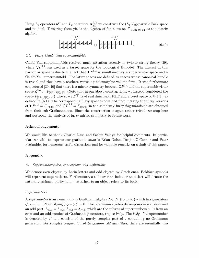
Using L1 operators aI† and L2 operators AIJ†2|0 we construct the (L1, L2)-particle Fock space

and its dual. Tensoring them yields the algebra of functions on F(1|0)(2|0);4|4 as the matrix

algebraL2+L1︷ ︸︸ ︷

• • • • • • • •• • • • ⊗

L2+L1︷ ︸︸ ︷

. (6.19)

6.5. Fuzzy Calabi-Yau supermanifolds

Calabi-Yau supermanifolds received much attention recently in twistor string theory [39],

where CP 3|4 was used as a target space for the topological B-model. The interest in this

particular space is due to the fact that CP 3|4 is simultaneously a supertwistor space and a

Calabi-Yau supermanifold. The latter spaces are defined as spaces whose canonical bundle

is trivial and thus have a nowhere vanishing holomorphic volume form. It was furthermore

conjectured [39, 40] that there is a mirror symmetry between CP 3|4 and the superambitwistor

space L5|6 := F(1|0)(3|3);4|3. (Note that in our above constructions, we instead considered the

space F(1|0)(3|4);4|4.) The space L5|6 is of real dimension 10|12 and a coset space of U(4|3), as

defined in (5.1). The corresponding fuzzy space is obtained from merging the fuzzy versions

of CP 3|3 = F1|0;4|3 and CP 3|3∗ = F3|3;4|3 in the same way fuzzy flag manifolds are obtained

from their sub-Graßmannians. Since the construction is again rather trivial, we stop here

and postpone the analysis of fuzzy mirror symmetry to future work.

Acknowledgements

We would like to thank Charles Nash and Sachin Vaidya for helpful comments. In partic-

ular, we wish to express our gratitude towards Brian Dolan, Denjoe O’Connor and Peter

Presnajder for numerous useful discussions and for valuable remarks on a draft of this paper.

Appendix

A. Supermathematics, conventions and definitions

We denote even objects by Latin letters and odd objects by Greek ones. Boldface symbols

will represent superobjects. Furthermore, a tilde over an index or an object will denote the

naturally assigned parity, and · attached to an object refers to its body.

Supernumbers

A supernumber is an element of the Graßmann algebra ΛN , N ∈ N∪∞which has generators

ξi, i = 1, . . . N satisfying ξiξj+ξjξi = 0. The Graßmann algebra decomposes into an even and

an odd part, ΛN,0 = ΛN,c, ΛN,1 = ΛN,a, which are the subsets of supernumbers built from an

even and an odd number of Graßmann generators, respectively. The body of a supernumber

is denoted by z and consists of the purely complex part of z containing no Graßmann

generator. For complex conjugation of Graßmann odd quantities, there are essentially two

42

conventions used throughout the literature. First, and most commonly, there is

(θ1θ2)∗ = θ2θ1 = −θ1θ2 , (A.1)

which is used e.g. in [38, 41]. Second, there is

(θ1θ2)∗ = −θ2θ1 = +θ1θ2 , (A.2)

which is used in [34, 42]. The latter convention respects the sign rule that interchanging two

Graßmann-odd objects in a monomial should always be accompanied by an additional sign.

There is a discussion of this issue in [42]. Manin in his book [32] also discusses all of these

conventions. In this paper, we use the second convention.

Supervectors

A supervector space is a free module over a supercommutative ring. We restrict our consid-

erations to supervector spaces which are endowed with a so-called pure basis. In particular,

consider a supervector space V with a so-called class I (even) basis (eA) of n even and ν

odd elements: (eA) = (e1, . . . , en, ε1, . . . , εν). The supervector space V is then said to be of

dimension n|ν.A n|ν-dimensional supervector consists of n+ ν components. If the first n of the compo-

nents of a supervector are even and the remaining ν odd, the supervector is called even. If

the inverse statement is true, the supervector is said to be odd:

x = xaea + ξαεα ⇒ x = 0 and x = ξaea + xαεα ⇒ x = 1 , (A.3)

where xi and ξi are complex even and odd supernumbers, respectively. If the supervector is

neither odd nor even, it is of mixed parity.

We will also allow for class II bases, in which the parity of the even and odd basis

elements is interchanged: (eA) = (ε1, . . . , εn, e1, . . . , eν). Here, the dependence of the parity

of a supervector on the parity of its components is evidently inverted.

Two supervectors (eA1 ), (eA

2 ) are called linearly independent, if and only if

αeA1 + βeA

2 = 0 ⇒ α = β = 0 , (A.4)

where α, β ∈ ΛN . This is equivalent to their bodies e1, e2 being linearly independent. A

scalar product between two complex supervectors is supposed to be graded antilinear, i.e.

(a,b) = (−1)ab(b,a)∗ . (A.5)

For even supervectors with components a = (ai, ηα) and b = (bi, ζα), where ai, bi ∈ ΛN,c and

ηα, ζα ∈ ΛN,a, we can thus define

(a,b) := a†b := aibi + iηαζα . (A.6)

Two supervectors are perpendicular, if they have nonvanishing bodies and the scalar product

between them vanishes. It follows that they are linearly independent.

43

A general supermatrix acting on the elements of an n|ν-dimensional supervector space is

of the block form

M =

(A B

C D

)

, (A.7)

where A is of dimension n×n and D of dimension ν× ν. The supermatrix M is called even,

if A and D have only even components and B and C consist only of odd components; it thus

preserves the parity of any supervector it acts on. Furthermore, if it inverts the parity of the

supervector, it is called odd.

Note that the space Cn|ν is defined in two different ways throughout the literature. Most

commonly, it denotes a space described by a set of coordinates consisting of n even and com-

plex numbers and ν complex Graßmann variables. On the other hand, it is a n|ν-dimensional

supervector space over a complex supercommutative ring, as e.g. the ring of complex super-

numbers. For the description of flag supermanifolds, we need the latter definition.

The supergroup U(4|4)

In our conventions for supergroups, we follow essentially [38], see also [43]. The Lie superal-

gebra u(n|ν) is given by block supermatrices of the form (A.7), where A and D are elements

of u(n) and u(ν), respectively, while B and C are hermitian conjugates of each other. This

algebra is generated by n2 + ν2 generators for the components A and C, which are even

supermatrices, as well as 2nν generators for the components B and C, which are odd su-

permatrices. Exponentiating these generators with even and odd parameters, respectively,

yields the supergroup U(n|ν). To obtain the superanalogue of su(n|ν), one linearly combines

the identities λ0n and λ0

ν of u(n) and u(ν) into

(1√n1n 0

0 1√ν1ν

)

and

(1√n1n 0

0 − 1√ν1ν

)

. (A.8)

Imposing the condition str (·) = 0 on the generators, eliminates the second generator. For

n 6= ν, this yields a semisimple super Lie algebra su(n|ν). For n = ν, however, the first factor

becomes 1n12n and generates an invariant Abelian subgroup. For this reason, one excludes

this generator and arrives at psu(n|n). However, the lowest dimensional representation is the

adjoint, see e.g. [38, 41] for more details. To avoid these complications, we choose to work

with u(4|4).The Killing form for u(n|n) is easily evaluated to be

gAB := str (λAλB) =

1n 0 0

0 1ν

−σ2 0 0

0 0 −σ2 0

0 0. . .

AB

, (A.9)

and we also define gAB with gABgBC = δC

A. The Killing form is furthermore supersymmetric,

i.e. gAB = (−1)˜A

˜BgBA and non-degenerate.

44

Supermanifolds

We define a (complex) supermanifold as a topological space X together with a sheaf ON ofZ2-graded supercommutative rings on X, satisfying the following two conditions

(i) There is a projection on the “body” of X, which is an ordinary complex manifold

of dimension m. More explicitly, consider the reduced structure sheaf O := ON/I,where I is the ideal of nilpotent elements in ON . We demand that (X,O) is a complex

manifold of dimension m.

(ii) Locally, the structure sheaf is the structure sheaf of the body with values in a Graßmann

algebra. That is, for every point x in X, there is an open neighborhood U such that

ON |U ∼= Ored|U (Λ∗Cn) . (A.10)

We will define the dimension of such a supermanifold to be m|n. For more details on super-

manifolds, see [32, 34, 41].

Riemannian supergeometry

A supermetric on a (real) supermanifold M := (M,ON ) is an ON -linear, even map g :

TM⊗ONTM satisfying the following properties:

(i) g is supersymmetric: g(X ⊗ Y ) = (−1)XY g(Y ⊗X).

(ii) g induces a Riemannian metric on (M,O).

(iii) g induces a symplectic form on the fermionic tangent directions of TM.

An almost complex structure on a (real) supermanifold M := (M,ON ) is an even, smooth

map I : TM → TM, which satisfies I2 = −1. As in ordinary complex geometry, a real

supermanifold underlying a complex supermanifold has a natural almost complex structure.

A hermitian supermetric on a supermanifold M := (M,ON ) with almost complex struc-

ture I is a supermetric g which satisfies g(IX ⊗ IY ) = g(X ⊗ Y ) for all vector fields X,Y in

TM. A Kahler supermetric is a supermetric, the derived Kahler form J(X,Y ) = g(X, IY )

of which is closed: dJ = 0. As an example of a Kahler supermanifold see the discussion of

the space CP 3|4 in section 5.5. For more details on supergeometry, see e.g. [44].

B. Representations of su(4) and u(4|4)

In this appendix, we briefly recall a few facts on the representation theory of su(4) and give

the necessary background on the superalgebra u(4|4) and its subalgebra su(4).

Representation of su(4) in terms of Plucker and embedding coordinates

Consider the case CP 3 ∼= SU(4)/U(3) ⊂ R16. A representation of SU(4) acting on functions

written in terms of complex Plucker coordinates ai ∈ C4 is given by

La = aiλaij

∂

∂aj− ajλa

ij

∂

∂ai, (B.1)

45

where λaij are again the Gell-Mann matrices of SU(4) together with the identity. One easily

verifies that [La,Lb] = i√

2fabcLc, where fab

c are the structure constants of SU(4). In terms

of the real coordinates

xa = aiλaija

j (B.2)

describing the canonical embedding of CP 3 in R16, the above generators read as

La = −i√

2fabcxb∂

∂xc, L0 ∼ xa ∂

∂xa. (B.3)

as one easily verifies. The representations in terms of the embedding coordinates for G2;4 is

given in the text, from which also the remaining cases follow.

Dynkin and Young diagrams for su(4)

The 15 generators of su(4) split into three generators of the Cartan subalgebraHi, i = 1, . . . , 3

and 12 raising and lowering operators E±~αj, j = 1, . . . 6 satisfying the commutation relations

[Hi,Hj ] = 0 , [Hi,E~α] = αiE~α ,

[E~α, E−~α] =∑

i

αiHi , [Eα, Eβ ] = NαβEα+β .(B.4)

Here, ~αj are the six three-dimensional positive root vectors, Σ+, three of which are simple.

The irreducible representations of su(4) can be labeled by the three eigenvalues µi of a highest

weight state |µ〉 under the action of the Hi. Equally well, one can label them by three integers

ai, the Dynkin labels, which are given by

ai = 2(~µ, ~αi)

(~αi, ~αi), (B.5)

where ~αi are the three simple roots. The Dynkin diagram labeling irreducible representations

of su(4) is then

i i ia1 a2 a3

(B.6)

and these representation are of dimension

d =a1 + 1

1

a2 + 1

1

a3 + 1

1

a1 + a2 + 2

2

a2 + a3 + 2

2

a1 + a2 + a3 + 3

3. (B.7)

The Dynkin labels indicate, how often one can act with a lowering operator on the highest

weight state without obtaining a trivial state:

(E−~αi)ai |µ〉 6= 0 , (E−~αi

)ai+1|µ〉 = 0 . (B.8)

On the other hand, the Dynkin labels appear naturally in the Young diagrams of the

representation (a1, a2, a3):a3+a2+a1︷ ︸︸ ︷

, (B.9)

and ai counts the number of columns with i boxes.

Due to the existence of the ε-tensor, which is invariant under SU(4), four antisymmetrized

boxes combine to a singlet. Furthermore, this tensor provides a duality between three anti-

symmetrized indices and one index as well as two antisymmetric ones and their complement:

φi = εijklφjkl and φij = 1

2εijklφkl . (B.10)

46

Schwinger construction for Lie superalgebras

Consider a Lie superalgebra having the even generators λa and the odd generators λα satis-

fying the commutation relations

[λa,λb] = fabcλ

c , [λa,λα] = faαβλβ , λα,λβ = fαβ

aλa . (B.11)

We summarize the generators into λA = (λa,λα) and the commutation relations to

[λA,λB ] = fABCλC , (B.12)

where [·] denotes the supercommutator. Assume furthermore that the generators are in a

representation acting on an (m|n)-dimensional supervector space. After introducing a set

of m bosonic and n fermionic oscillators together with the corresponding annihilation and

creation operators

aI = (ai, ηα) and aI† = (ai†, ηα†) , (B.13)

the Schwinger construction yields a representation of the Lie superalgebra by

LA = aI†λAIJ a

J . (B.14)

Representation of u(4|4) in terms of Plucker and embedding coordinates

Completely analogously to the representations of u(4) in terms of coordinates describingCP 3, one finds a representation of u(4|4) in terms of coordinates describing CP 3|4. We have

LA = aIλAIJ

∂

∂aJ− aJλA

IJ

∂

∂aI, (B.15)

where aI = (ai, ηα) ∈ C4|4 and in terms of the real coordinates

xA = aIλAIJa

J (B.16)

describing the embedding of CP 3|4 in R32|32, the above generators read as

LA = −i√

2fABCxB∂

∂xC, L0 ∼ xA ∂

∂xA. (B.17)

Representations and Dynkin diagrams for psu(4|4)

The representations of supergroups are divided into two classes. In the first class, the repre-

sentation space is spanned by an even basis, while in the second one, the basis is odd and they

can be regarded as dual to each other. Representations are again labelled by highest weights,

which are the eigenvalues of the generators of the Cartan subalgebra. The latter is generated

by two copies of the Cartan subalgebra of su(4) as well as H4 := diag(0, 0, 0, 1, 1, 0, 0, 0), cf.

section 6.1. Accordingly, the Dynkin diagram has seven nodes:

i i i i i i ia1 a2 a3 q0

×a4 a5 a6

(B.18)

It is now evident that a class I representation is dual to a class II representation provided

that

aIi = aII

7−i and qI0 = qII

0 . (B.19)

47

Since the superdeterminant is no longer a polynomial of finite degree, there is no invariant

totally antisymmetric ε-tensor for the SU(m|n) supergroups. However, the duality between

class I and II representation takes over the role of the duality between the representation and

the corresponding conjugate representation. The latter arises from the interchange between

covariant and contravariant indices corresponding to a contraction with an ε-tensor in the

SU(4) picture, as we saw above.

The second order Casimir operator on irreducible representations of su(4)

We constructed the algebra of functions on the fuzzy flag manifolds from spherical represen-

tations of the groups underlying the flag manifolds. These representations are described by

Young diagrams, and given such a Young diagram with m ≤ 4 rows of n1 ≥ . . . ≥ nm ≥ 0

boxes, the eigenvalue of the second order Casimir operator on these representations reads

as13

1

2

(

4

m∑

i=1

ni +

m∑

i=1

ni(ni + 1− 2i)− (∑m

i=1 ni)2

4

)

. (B.20)

We will be mostly interested in the representations consisting of a row of 2L boxes and 2

rows of L boxes. For these diagrams, the above formula reduces to L(L + 3). The other

type of diagrams we will encounter consist of three rows with a+ b + a, a+ b and a boxes,

respectively. For them, the above formula reduces to a2 + a(3 + b) + 12b(4 + b).

The second order Casimir operator on representations of u(n|n)

We can write the second order Casimir operator acting on the Hilbert space H F1|0;4|4 of CP 3|4

F

in terms of one set of oscillators using the Schwinger construction:

C2 = gABLALB

=n− 1

nNb(Nb + n) +

1

nN2

b −n+ 1

nNf (n− Nf )− 1

nN2

f + (2NbNf + nNf − nNb)

=1

2N(N− 1) ,

where Nb = ai†ai and Nf = ηα†ηα. For the other flag supermanifold we require more than

one set of oscillators and the calculation is more complicated.

Fierz and super Fierz identities

Consider the Gell-Mann matrices λa, a = 1, . . . , 15 of su(4) and extend them to the generators

λa of u(4) by adding λ0 = 1/√4. We have the Fierz identity

λaijλ

akl = δilδjk , (B.21)

which trivially extends in the case of the antisymmetric tensor products λab... := λa∧λb∧ . . .we defined in section 2.3 to

(λab)ij;kl(λab)mn;pq = (δipδkmδjqδln)[ij][kl][mn][pq] ,

(λabc)ijk;lmn(λabc)pqr;stu = (δisδlpδjtδmqδkuδnr)[ijk][lmn][pqr][stu] .(B.22)

13This formula is given, e.g., in [45] with a different normalization of the Lie algebra generators.

48

Moreover, we can write

tr (A1λa)λa = A1 and tr (A1λ

a)λa = A1 − 14 tr (A1)1 (B.23a)

for any hermitian matrix A1 ∈Mat4 as well as

tr (A2λab)λab = A2

tr (A3λabc)λabc = A3

(B.23b)

for hermitian matrices A2 ∈Mat4 ∧Mat4 and A3 ∈Mat4 ∧Mat4 ∧Mat4.

We can use the Killing form on U(4|4) to establish the following super Fierz identity:

gABλIJA

λKLB

= δILδJK . (B.24)

To prove this formula quickly, one can e.g. extend the one for SU(n|n) given in [38]. From

this Fierz identity, we can, as in the purely bosonic case, immediately derive the further

identities

(λAB)IJ ;KL(λAB)MN ;PQ = (δIP δKMδJQδLN )[IJ ][KL][MN ][PQ] ,

(λABC)IJK;LMN(λABC)PQR;STU = (δISδLP δJT δMQδKUδNR)[IJK][LMN ][PQR][STU ] ,

where λAB denotes again the graded antisymmetric tensor product

λAB = λA⋓ λB (B.25)

introduced in section 5.3.

Oscillator representation of internal isotropy subgroups

In the description of the various Graßmannians, we needed the following formula to describe

the action of the internal part of the isotropy subgroup acting on the states of certain Fock

spaces:

[(aip)

†λApqa

iq, a

[j1†1 . . . a

jk]†k ] = 0 . (B.26)

To prove this formula, consider the following form of the generators Lpq of U(k):

Lpq = ai†p a

iq , (B.27)

where i is summed over. The composite creation operators relevant in the description of Gk;n

can be written as

Ai1···ik†k =

1

k!ǫp1···pk

a[i1†p1· · · aik]†

pk. (B.28)

Then

[Lpq, Ai1···ik†k ] =

1

k!ǫp1···pk

ai†p [ai

q, a[i1†p1· · · aik]†

pk]

=1

k!

k∑

j=1

ǫp1···pkai†

p a[i1†p1· · · δiijδqpj

· · · aik]†pk

=k

k!ǫqp2···pk

a[i1†p ai2†

p2· · · aik]†

pk

= δpqAi1···ik†k ,

49

and thus the (traceless) generators of SU(k) leave the composite creation operators invariant.

In the supersymmetric case, the same statement holds. Here, the creation and annihila-

tion operators satisfy

[aIp,a

J†q ] = δpqδ

IJ . (B.29)

Using the relations

[a,bc] = [a,b]c + (−1)abb[a, c] ,[ab, c] = a[bc] + (−1)bc[a, c]b ,

(B.30)

we obtain

[aIp, A

JK†2|0 ] = [aI

p,aJ†1 ]aK†

2 + (−1)I JaJ†1 [aI

p,aK†2 ] − (−1)J K(J ↔ K)

= δp1δIJa

K†2 + δp2(−1)I JδIKa

J†1 − (−1)J K(J ↔ K) .

(B.31)

With this relation, we can conclude that

[aI†p aI

q ,AJK†2|0 ] = aI†

p [aIq ,A

JK†2|0 ]

= δq1(aJ†p a

K†2 − (−1)J KaK†

p aJ†2 ) + δq2((−1)KJaK†

p aJ†1 − aJ†

p aK†1 )

= δp1δq1AJK†2|0 + δp2δq2A

JK†2|0

= δpqAJK†2|0 .

(B.32)

Similar relations can also be proven for the remaining cases of A2|4 and A3|4 by observing

that, for example,

AJKL†3|0 = A

JK†2|0 a

L†3 − (−1)KLA

JL†2|0 a

K†3 + (−1)J K+JLA

KL†2|0 a

J†3 (B.33)

and

[aI†p aI

q ,AJK†2|0 a

L†3 ] = [aI†

p aIq ,A

JK†2|0 ]aL†

3 + AJK†2|0 [aI†

p aIq ,a

L†3 ] (B.34)

= (δpq − δp3δq3)AJK†2|0 a

L†3 + δq3A

JK†2|0 aL†

p . (B.35)

Hence,

[aI†p aI

q ,AJKL†3|0 ] = δpqA

JKL†3|0 . (B.36)

References

[1] J. Madore, The fuzzy sphere, Class. Quant. Grav. 9 (1992) 69;

[2] J. Hoppe, Quantum theory of a massless relativistic surface and a two-dimensional bound

state problem, PhD Thesis, MIT, 1982, http://www.aei.mpg.de/∼hoppe/; A. P. Bal-

achandran, Quantum spacetimes in the year 1, Pramana 59 (2002) 359 [hep-th/0203259].

[3] H. Grosse, C. Klimcik, and P. Presnajder, Towards finite quantum field theory in non-

commutative geometry, Int. J. Theor. Phys. 35 (1996) 231 [hep-th/9505175]; H. Grosse

and A. Strohmaier, Noncommutative geometry and the regularization problem of 4D

quantum field theory, Lett. Math. Phys. 48 (1999) 163 [hep-th/9902138]; B. P. Dolan,

D. O’Connor, and P. Presnajder, Matrix φ4 models on the fuzzy sphere and their con-

tinuum limits, JHEP 03 (2002) 013 [hep-th/0109084].

50

[4] A. P. Balachandran, X. Martin, and D. O’Connor, Fuzzy actions and their continuum

limits, Int. J. Mod. Phys. A 16 (2001) 2577 [hep-th/0007030].

[5] A. P. Balachandran, B. P. Dolan, J.-H. Lee, X. Martin, and D. O’Connor, Fuzzy complex

projective spaces and their star-products, J. Geom. Phys. 43 (2002) 184 [hep-th/0107099].

[6] B. Ydri, Fuzzy physics, hep-th/0110006.

[7] B. P. Dolan and O. Jahn, Fuzzy complex Grassmannian spaces and their star products,

Int. J. Mod. Phys. A 18 (2003) 1935 [hep-th/0111020].

[8] S. Baez, A. P. Balachandran, B. Ydri, and S. Vaidya, Monopoles and solitons in fuzzy

physics, Commun. Math. Phys. 208 (2000) 787 [hep-th/9811169]; A. P. Balachandran

and S. Vaidya, Instantons and chiral anomaly in fuzzy physics, Int. J. Mod. Phys. A

16 (2001) 17 [hep-th/9910129]; G. Alexanian, A. P. Balachandran, G. Immirzi, and

B. Ydri, Fuzzy CP 2, J. Geom. Phys. 42 (2002) 28 [hep-th/0103023]; B. P. Dolan and

C. Nash, Chiral fermions and Spin(C) structures on matrix approximations to manifolds,

JHEP 07 (2002) 057 [hep-th/0207007].

[9] S. Vaidya, Perturbative dynamics on fuzzy S2 and RP 2, Phys. Lett. B 512 (2001) 403

[hep-th/0102212]; H. Grosse, C. Klimcik, and P. Presnajder, Finite quantum field theory

in noncommutative geometry, Commun. Math. Phys. 180 (1996) 429 [hep-th/9602115].

[10] S. Ramgoolam, On spherical harmonics for fuzzy spheres in diverse dimensions, Nucl.

Phys. B 610 (2001) 461 [hep-th/0105006]; Y. Kimura, Noncommutative gauge theory

on fuzzy four-sphere and matrix model, Nucl. Phys. B 637 (2002) 177 [hep-th/0204256];

B. P. Dolan and D. O’Connor, A fuzzy three sphere and fuzzy tori, JHEP 10 (2003) 060

[hep-th/0306231]; B. P. Dolan, D. O’Connor, and P. Presnajder, Fuzzy complex quadrics

and spheres, JHEP 02 (2004) 055 [hep-th/0312190].

[11] A. P. Balachandran, S. Kurkcuoglu, and S. Vaidya, Lectures on fuzzy and fuzzy SUSY

physics, hep-th/0511114.

[12] C. Klimcik and P. Severa, Open strings and D-branes in WZNW models, Nucl. Phys.

B 488 (1997) 653 [hep-th/9609112]; H. Garcia-Compean and J. F. Plebanski, D-

branes on group manifolds and deformation quantization, Nucl. Phys. B 618 (2001)

81 [hep-th/9907183].

[13] A. Y. Alekseev, A. Recknagel, and V. Schomerus, Non-commutative world-volume ge-

ometries: Branes on SU(2) and fuzzy spheres, JHEP 09 (1999) 023 [hep-th/9908040].

[14] R. C. Myers, Dielectric-branes, JHEP 12 (1999) 022 [hep-th/9910053].

[15] S. P. Trivedi and S. Vaidya, Fuzzy cosets and their gravity duals, JHEP 09 (2000) 041

[hep-th/0007011]; S. R. Das, S. P. Trivedi, and S. Vaidya, Magnetic moments of branes

and giant gravitons, JHEP 10 (2000) 037 [hep-th/0008203].

51

[16] A. F. Kleppe and C. Wainwright, Super coset space geometry, hep-th/0610039.

[17] G. Gotz, T. Quella, and V. Schomerus, The WZNW model on PSU(1, 1|2),hep-th/0610070.

[18] P. S. Howe and G. G. Hartwell, A superspace survey, Class. Quant. Grav. 12 (1995)

1823.

[19] A. D. Popov and C. Saemann, On supertwistors, the Penrose-Ward transform and N = 4

super Yang-Mills theory, Adv. Theor. Math. Phys. 9 (2005) 931 [hep-th/0405123].

[20] Brian P. Dolan, I. Huet, S. Murray and D. O’Connor, “Noncommutative vector

bundles over fuzzy CP(N) and their covariant derivatives,” JHEP 07 (2007) 007

[hep-th/0611209].

[21] M. Aganagic and C. Vafa, Mirror symmetry and supermanifolds, hep-th/0403192;

S. P. Kumar and G. Policastro, Strings in twistor superspace and mirror symmetry,

Phys. Lett. B 619 (2005) 163 [hep-th/0405236].

[22] R. F. Picken, The Duistermaat-Heckman integration formula on flag manifolds, J. Math.

Phys. 31 (1990) 616.

[23] L. J. Mason and N. M. J. Woodhouse, Integrability, self-duality, and twistor theory,

Clarendon, Oxford (1996).

[24] A. Cucchieri, T. Mendes, and A. Pelissetto, Pseudo-character expansions for U(N)-

invariant spin models on CPN−1, Ann. Comb. 3 (1999) 287 [hep-lat/9810027].

[25] P. B. Gilkey, J. V. Leahy, and J. Park, Spinors, spectral geometry and Riemannian

submersions, Global Analysis Research Center of Seoul National University (1998).

[26] S. Helgason, Groups and geometric analysis, Acad. Press (1984).

[27] M. S. Dijkhuizen, Some remarks on the construction of quantum symmetric spaces,

math.QA/9512225.

[28] A. M. Perelomov, Generalized coherent states and their applications, Springer, Berlin

(1986).

[29] M. Chaichian, D. Ellinas, and P. Presnajder, Path integrals and supercoherent states,

J. Math. Phys. 32 (1991) 3381. H. Grosse and P. Presnajder, The construction on

noncommutative manifolds using coherent states, Lett. Math. Phys. 28 (1993) 239.

[30] A. M. Perelomov, Description of generalized coherent states closest to classical states

(in Russian), Yad. Fiz. 29 (1979) 1688.

[31] S. Kurkcuoglu and C. Saemann, “Drinfeld twist and general relativity with fuzzy spaces,”

Class. Quant. Grav. 24 (2007) 291 [hep-th/0606197].

52

[32] Y. I. Manin, Gauge field theory and complex geometry, Grundlehren der mathematischen

Wissenschaften, 289, Springer (1988).

[33] S. Kleiman and D. Laksov, Schubert Calculus, Amer. Math. Monthly 79 (1972) 1061.

[34] P. Cartier, C. DeWitt-Morette, M. Ihl, C. Saemann, and M. E. Bell, Supermanifolds -

Application To Supersymmetry, math-ph/0202026. in: “Multiple facets of quantization

and supersymmetry: Michael Marinov memorial volume”, Eds. M. Olshanetsky and

A. Vainshtein, World Scientific (2002).

[35] C. Klimcik, An extended fuzzy supersphere and twisted chiral superfields, Commun.

Math. Phys. 206 (1999) 587 [hep-th/9903202].

[36] E. Ivanov, L. Mezincescu and Paul K. Townsend, “Fuzzy CP (n|m) as a quantum su-

perspace,” hep-th/0311159; “A super-flag Landau model,” hep-th/0404108; “Planar

super-Landau models,” JHEP 01 (2006) 143 [hep-th/0510019].

[37] I. Bars, B. Morel, and H. Ruegg, Kac-Dynkin diagrams and supertableaux, J. Math.

Phys. 24 (1983) 2253.

[38] I. Bars, Supergroups and their representations, Lectures Appl. Math. 21 (1983) 17.

[39] E. Witten, Perturbative gauge theory as a string theory in twistor space, Commun. Math.

Phys. 252 (2004) 189 [hep-th/0312171].

[40] M. Aganagic and C. Vafa, Mirror symmetry, D-branes and counting holomorphic discs,

hep-th/0012041.

[41] B. S. DeWitt, Supermanifolds, 2nd ed., Cambridge University Press, Cambridge (1992).

[42] P. Deligne, P. Etingof, D. Freed, L. Jeffrey, D. Kazhdan, J. Morgan, D. Morrison, and

E. Witten, Quantum fields and strings: A course for mathematicians, AMS, Providence

(1999).

[43] V. G. Kac, Representations of classical Lie superalgebras, in: “Differential Geometrical

Methods in Mathematical Physics II”, Lectures Notes in Mathematics 676, Springer

(1978).

[44] S. Varsaie, Kahlerian supermanifolds, Journal of Mathematical Physics 40 (1999) 6701.

[45] D. J. Gross, Two-dimensional QCD as a string theory, Nucl. Phys. B 400 (1993) 161

[hep-th/9212149].

53