higher fano manifolds - INMABB

REVISTA DE LA UNION MATEMATICA ARGENTINAVol. 64, No. 1, 2022, Pages 103–125Published online: May 10, 2022https://doi.org/10.33044/revuma.2921

HIGHER FANO MANIFOLDS

CAROLINA ARAUJO, ROYA BEHESHTI, ANA-MARIA CASTRAVET,KELLY JABBUSCH, SVETLANA MAKAROVA, ENRICA MAZZON, LIBBY TAYLOR,

AND NIVEDITA VISWANATHAN

Abstract. We address in this paper Fano manifolds with positive higherChern characters, which are expected to enjoy stronger versions of several ofthe nice properties of Fano manifolds. For instance, they should be coveredby higher dimensional rational varieties, and families of higher Fano manifoldsover higher dimensional bases should admit meromorphic sections (modulothe Brauer obstruction). Aiming at finding new examples of higher Fanomanifolds, we investigate positivity of higher Chern characters of rationalhomogeneous spaces. We determine which rational homogeneous spaces ofPicard rank 1 have positive second Chern character, and show that the onlyrational homogeneous spaces of Picard rank 1 having positive second andthird Chern characters are projective spaces and quadric hypersurfaces. Wealso classify Fano manifolds of large index having positive second and thirdChern characters. We conclude by discussing conjectural characterizations ofprojective spaces and complete intersections in terms of these higher Fanoconditions.

1. Introduction

Fano manifolds are complex projective manifolds having positive first Chernclass c1(TX). Examples of Fano manifolds include projective spaces, smooth com-plete intersections of low degree in projective spaces, and rational homogeneousspaces. The positivity condition on the first Chern class has far reaching geometricand arithmetic implications, making Fano manifolds a central subject in algebraicgeometry. To illustrate the special role played by Fano manifolds, we briefly discusssome of their nice properties.

Hypersurfaces of low degree in projective spaces provide basic examples of Fanomanifolds. The first Chern class of a smooth hypersurface Xd ⊂ Pn+1 of degreed ≥ 1 is given by

c1(TXd) = c1

(OXd

(n+ 2− d)).

Therefore, Xd ⊂ Pn+1 is Fano if and only if d ≤ n+ 1. One can easily check that ifd ≤ n, then Xd is covered by lines, and if d = n+ 1, then Xd is covered by conics.

2020 Mathematics Subject Classification. 14M17.

103

https://doi.org/10.33044/revuma.2921

104 CAROLINA ARAUJO ET AL.

In contrast, if d ≥ n+ 2, then through a general point of Xd there are no rationalcurves. Hence, for smooth hypersurfaces in projective spaces:

Xd ⊂ Pn+1 is Fano ⇐⇒ d ≤ n+ 1 ⇐⇒ Xd is covered by rational curves.In the landmark paper [32], Mori showed that any Fano manifold is covered by

rational curves. Since then, rational curves have become a fundamental tool in thestudy of Fano manifolds. Later, it was proved in [25] and [6] that a much strongerproperty holds: any Fano manifold X is rationally connected, i.e., there are rationalcurves connecting any two points of X.

Fano hypersurfaces also satisfy special arithmetic properties, as illustrated bythe classical Tsen’s theorem, which states that a hypersurface X ⊂ Pn+1

K of degreed ≤ n+ 1 over the function field K of a curve always has a K-point. In geometricterms, Tsen’s theorem says that families of hypersurfaces of degree d ≤ n + 1 inPn+1 over one dimensional bases always admit holomorphic sections. This resulthas been greatly generalized by Graber, Harris and Starr in [17]. They showedthat proper families of rationally connected varieties over curves always admitholomorphic sections.

In [29], Lang provided a version of Tsen’s theorem for function fields of higherdimensional varieties.Theorem (Tsen–Lang Theorem). Let K be the function field of a variety of di-mension r ≥ 1. If X ⊂ Pn+1

K is a hypersurface of degree d with dr ≤ n+ 1, then Xhas a K-point.

As before, this statement can be interpreted as saying that families of hyper-surfaces of degree d in Pn+1 over r-dimensional bases always admit meromorphicsections provided that dr ≤ n + 1. A natural problem consists in finding naturalgeometric conditions on general fibers of a fibration π : X → B over a higher di-mensional base under which the conclusion on the Tsen–Lang theorem holds. Wenote, however, that over higher dimensional bases, in addition to conditions on thefibers of the family, one must observe the existence of Brauer obstruction on thebase. We do not address the latter here, and refer to [41] for a discussion on theBrauer obstruction in connection with the Tsen–Lang theorem.

In recent years, there has been great effort towards defining suitable higheranalogues of the Fano condition. Higher Fano manifolds are expected to enjoystronger versions of several of the nice properties of Fano manifolds.Problem 1.1. Find natural geometric conditions Rr on a manifold X such that:

- for hypersurfaces Xd ⊂ Pn+1, the condition Rr is equivalent to dr ≤ n+ 1;- if a complex projective manifold satisfies Rr, then X is covered by rational

varieties of dimension r; and- families of projective manifolds satisfying Rr over r-dimensional bases al-

ways admit meromorphic sections (modulo Brauer obstruction).For r = 1, it follows from the previous discussion that the condition R1 can

be taken to be “X is rationally connected,” or, more restrictively, “X is a Fanomanifold.”

Rev. Un. Mat. Argentina, Vol. 64, No. 1 (2022)

HIGHER FANO MANIFOLDS 105

In a series of papers, De Jong and Starr introduce and investigate possiblecandidates for the condition R2 ([40], [11], [12], [13], [10]). They present somenotions of rationally simple connectedness, inspired by the natural analogue ofProblem 1.1 in topology. Namely, let π : M → B be a fibration of CW complexeswith typical fiber F over an r-dimensional base B. If F is (r − 1)-connected,then π admits a continuous section s : B → M . If one draws a parallel betweentopology and algebraic geometry, interpreting a loop as a rational curve, one getsthat the solution of the problem for r = 1 in topology, namely F is path-connected,translates precisely into the condition that the general fiber of the fibration π : X →B is rationally connected. For r > 1, this analogy has limitations, and De Jongand Starr’s notions of rationally simple connectedness are technical and hard tocheck in practice. Roughly speaking, and at the very least, one asks that a suitableirreducible component of the scheme of rational curves through two general pointsof X is itself rationally connected. This notion led to a version of the Tsen–Lang theorem for fibrations by rationally simply connected manifolds over surfacesin [10]. More recently, other notions of rationally simple connectedness have beeninvestigated, for example in [14].

In [11], De Jong and Starr introduced 2-Fano manifolds as an alternative can-didate to the condition R2. A projective manifold X is said to be 2-Fano if it isFano and the second Chern character ch2(TX) = 1

2c1(TX)2 − c2(TX) is positive,i.e., ch2(TX) · S > 0 for every surface S in X. This condition conjecturally impliesrationally simple connectedness, but it is much easier to check. In [13], it is shownthat 2-Fano manifolds satisfying some mild assumptions are covered by rationalsurfaces.

In [2], Araujo and Castravet introduced a new approach to study 2-Fano mani-folds, via polarized minimal families of rational curves (Hx, Lx). For a Fano mani-fold X and a point x ∈ X, let Hx be a proper irreducible component of the schemeRatCurvesn(X,x), parametrizing rational curves on X through x having minimalanti-canonical degree. If x is a general point of X, then every such componentis smooth and comes with a finite and birational morphism τx : Hx → P(TxX∗),mapping a point parametrizing a smooth curve at x to its tangent direction at x.Consider the polarization Lx := τ∗xO(1) on Hx. Then [2, Proposition 1.3] gives aformula for all Chern characters of Hx in terms of the Chern characters of X andc1(Lx). As a consequence, if X is 2-Fano and dim(Hx) ≥ 1, then Hx is Fano. Ifmoreover ch3(X) > 0 and dim(Hx) ≥ 2, then Hx is 2-Fano. This motivates thefollowing definition.Definition 1.2. We say that a Fano manifold X satisfies the condition Fr if itsChern characters chi(X) are positive for all 1 ≤ i ≤ r. This positivity conditionmeans that chi(TX) · Z > 0 for every effective i-cycle Z in X.

Given a Fano manifold X satisfying condition Fr and a polarized minimal familyof rational curves (Hx, Lx) on it, one can ask whether Hx satisfies condition Fr−1.We note the analogy with the higher notions of connectedness in topology: if apath-connected topological space M is r-connected, then its loop spaces (with thecompact-open topology) are (r − 1)-connected.



The inductive approach introduced in [2] was further explored in [42] and [33]to show that, under some extra assumptions, Fano manifolds satisfying conditionFr are covered by rational r-folds.

Despite these recent developments, few examples of higher Fano manifolds areknown. The strong restrictions on (Hx, Lx) imposed by the 2-Fano condition ex-plain why examples are difficult to find, but they also suggest where to look forthem. Following this trail, new examples of 2-Fano manifolds were described in [2],including several homogeneous and quasi-homogeneous spaces. A few more exam-ples were presented in [3], where Araujo and Castravet classified 2-Fano manifoldswith large index.

The present paper addresses the problem of finding new examples of higherFano manifolds. We start by investigating rational homogeneous spaces, for whichthe polarized minimal families of rational curves are well described in [27]. Thissearch provides new examples of 2-Fano manifolds of exceptional type E and F(see Section 3 for the notation regarding rational homogeneous spaces), and yieldsthe following classification of 2-Fano rational homogeneous spaces of Picard rank 1.Rational homogeneous spaces of higher Picard rank will be addressed in a forth-coming paper.Theorem 1.3. The following is the complete list of rational homogeneous spacesof Picard rank 1 satisfying the condition F2:

- An/P k, for k = 1, n and for n = 2k − 1, 2k when 2 ≤ k ≤ n+12 ;

- Bn/P k, for k = 1, n and for 2n = 3k + 1 when 2 ≤ k ≤ n− 1;- Cn/P k, for k = 1, n and for 2n = 3k − 2 when 2 ≤ k ≤ n− 1;- Dn/P

k, for k = 1, n− 1, n and for 2n = 3k + 2 when 2 ≤ k < n− 1;- En/P k, for n = 6, 7, 8 and k = 1, 2, n;- F4/P

4;- G2/P

k, for k = 1, 2.

However, we get no new examples of Fano manifolds satisfying F3:Theorem 1.4. The only rational homogeneous spaces of Picard rank 1 satisfyingF3 are projective spaces Pn, n ≥ 3, and quadric hypersurfaces Qn ⊂ Pn+1, n ≥ 7.

Next we go through the list of 2-Fano manifolds with large index in [3] and checkthe F3 condition for those. We obtain the following classification.Theorem 1.5. Let X be a Fano manifold of dimension n ≥ 3 and index iX ≥ n−2.If X satisfies F3, then X is isomorphic to one of the following:

• Pn.• Complete intersections in projective spaces:

- Quadric hypersurfaces Qn ⊂ Pn+1 with n > 6;- Complete intersections of quadrics X2·2 ⊂ Pn+2 with n > 13;- Cubic hypersurfaces X3 ⊂ Pn+1 with n > 25;- Quartic hypersurfaces in Pn+1 with n > 62;- Complete intersections X2·3 ⊂ Pn+2 with n > 32;- Complete intersections X2·2·2 ⊂ Pn+3 with n > 20.



• Complete intersections in weighted projective spaces:- Degree 4 hypersurfaces in P(2, 1, . . . , 1) with n > 55;- Degree 6 hypersurfaces in P(3, 2, 1, . . . , 1) with n > 181;- Degree 6 hypersurfaces in P(3, 1, . . . , 1) with n > 188;- Complete intersections of two quadrics in P(2, 1, . . . , 1) with n > 6.

So the following remains an open problem.

Problem 1.6. Find examples of Fano manifolds satisfying condition F3 other thancomplete intersections in weighted projective spaces.

Our results show that conditions Fr for r ≥ 3 are extremely restrictive, and leadto conjectural characterizations of projective spaces and complete intersections interms of positivity of Chern characters. It has already been asked in [2] whetherthe only n-dimensional Fano manifold satisfying Fn is the projective space Pn. Webelieve that a much stronger statement holds.

Conjecture 1.7. If X is an n-dimensional Fano manifold satisfying condition Fk,with k = dlog2(n+ 1)e, then X ∼= Pn.

Problem 1.8. For fixed n, find the smallest integer k = k(n) such that the fol-lowing holds. If X is an n-dimensional Fano manifold satisfying condition Fk, thenX is a complete intersection in a weighted projective space. Can this integer k bechosen independently of n?

Throughout this paper we work over C.The paper is organized as follows. In Section 2, we review the basic theory of

minimal families of rational curves on Fano manifolds, and discuss their specialproperties when the ambient space satisfies higher Fano conditions. In Section 3,we provide a background on rational homogeneous spaces. In Sections 4 and 5,we go through the classification of rational homogeneous spaces of classical andexceptional types, and check conditions F2 and F3. This case-by-case analysis willprove Theorems 1.3 and 1.4. In Section 6, we prove Theorem 1.5.

Acknowledgements. This paper anchors the invited lecture of Carolina Araujoat the Mathematical Congress of the Americas 2021. She thanks the MathematicalCouncil of the Americas and the organizers of the congress for the opportunity.This work grew from the “Women in Algebraic Geometry Collaborative ResearchWorkshop”, a working group at the ICERM, in July 2020. We thank ICERM for thesupport and opportunity to start this research collaboration. We have also beenfunded by the NSF-ADVANCE Grant 150048, Career Advancement for Womenthrough Research-focused Networks. We thank AWM for this support. CarolinaAraujo was partially supported by CNPq and Faperj Research Fellowships. Ana-Maria Castravet was partially supported by the grant ANR-20-CE40-0023. EnricaMazzon was partially supported by the Max Planck Institute for Mathematics. Theauthors thank Aravind Asok, Laurent Manivel, Mirko Mauri, and Nicolas Perrinfor several enlightening discussions and comments.



2. Minimal rational curves on higher Fano manifolds

In this section, we discuss special properties of minimal families of rationalcurves on higher Fano manifolds. We start by reviewing the basic properties ofminimal families of rational curves. We refer to [24, Chapters I and II] for thebasic theory of rational curves on complex projective varieties.

LetX be a Fano manifold and x ∈ X a point. There is a scheme RatCurvesn(X,x)that parametrizes rational curves on X through x. It can be constructed asthe normalization of a certain subscheme of the Chow variety Chow(X), whichparametrizes effective 1-cycles on X (see [24, II.2.11]). The superscript n inRatCurvesn(X,x) stands for the normalization. Let Hx be a proper irreduciblecomponent of RatCurvesn(X,x). We call it a minimal family of rational curvesthrough x. For instance, one can take Hx to be an irreducible component ofRatCurvesn(X,x) parametrizing rational curves through x, having minimal de-gree with respect to −KX . If x ∈ X is a general point, then Hx is smooth. Fromthe universal properties of Chow(X), we get the universal family diagram

Ux X,

Hx

ev

π

where π is a P1-bundle.The variety Hx comes with a natural finite morphism τx : Hx → P(TxX∗)

sending a curve that is smooth at x to its tangent direction at x (see [23, Theorems3.3 and 3.4]). The morphism τx is also birational by [21]. Set Lx := τ∗xO(1). Thepair (Hx, Lx) is called a polarized minimal family of rational curves through x.

In [2], Araujo and Castravet computed all the Chern characters of Hx in termsof the Chern characters of X and c1(Lx). In order to state the result, first wedefine, for any k ≥ 1:

T := π∗ev∗ : Nk(X)R → Nk−1(Hx)R.

By [2, Proposition 1.3],

chk(Hx) =k∑j=0

Ajc1(Lx)j · T (chk+1−j(X))− 1k!c1(Lx)k, (2.1)

where Aj = (−1)jBj

j! and the Bj ’s are the Bernoulli numbers.Set d := dim(Hx) and η := T (ch2(X))− Lx

2 . Then, for 1 ≤ k ≤ 3, (2.1) becomes:

c1(Hx) = T (ch2(X)) + d

2 c1(Lx)

ch2(Hx) = T (ch3(X)) + 12

(c1(Hx)− d

2 c1(Lx))Lx + d− 4

12 L2x (2.2)



ch3(Hx) = T (ch4(X)) + 12T (ch3(X)) · Lx + 1

12T (ch2(X)) · L2x −

16L

3x

= T (ch4(X)) + 12T (ch3(X)) · Lx + L2

x

12

(η − 3

2Lx).

(2.3)

Using the fact that the map T : Nk(X)R → Nk−1(Hx)R preserves positivity fork − 1 ≤ d ([2, Lemma 2.7]), it is possible to show an inductive structure on theclass of higher Fano manifolds.

Theorem 2.1. Let X be a Fano manifold, and (Hx, Lx) a polarized minimal familyof rational curves through a general point x ∈ X.

(1) ([2, Theorem 1.4 (2)]) If X satisfies F2 and d ≥ 1, then Hx satisfies F1(i.e., it is a Fano manifold).

(2) ([2, Theorem 1.4 (3)]) If X satisfies F3 and d ≥ 2, then Hx satisfies F2 andρ(Hx) = 1.

(3) If X satisfies F4, d ≥ 3 and η ≥ 32Lx, then Hx satisfies F3 and ρ(Hx) = 1.

Proof of (3). Suppose that the Fano manifold X satisfies F4, d ≥ 3 and η ≥ 32Lx.

We know from (2) that Hx is a Fano manifold satisfying F2 and ρ(Hx) = 1. Usingthe fact that the map T : Nk(X)R → Nk−1(Hx)R preserves positivity for k−1 ≤ d,it follows from (2.3) that ch3(Hx) > 0, and thus Hx satisfies F3. �

Remark 2.2. Let the assumptions be as in Theorem 2.1 (3). By [2, Proof ofTheorem 1.4, p. 99], the class η is nef. Since both 2η and 2 · ch2(X) are integralclasses, the assumption η ≥ 3

2Lx is satisfied, except if η = 0, 12Lx, Lx.

We end this section with the description of (Hx, Lx) when X is a Fano manifoldsatisfying F2.

Theorem 2.3 ([2, Theorem 1.4 (2)]). Let X be a Fano manifold, (Hx, Lx) a po-larized minimal family of rational curves through a general point x ∈ X, and setd = dimHx.

(1) If X is 2-Fano, then Hx is a Fano manifold with Pic(Hx) = Z · [Lx], exceptif (Hx, Lx) is isomorphic to one of the following:(a)

(Pm × Pm, p∗

1O(1)⊗ p∗

2O(1)

), with d = 2m,

(b)(Pm+1 × Pm, p∗

1O(1)⊗ p∗

2O(1)

), with d = 2m+ 1,

(c)(PPm+1

(O(2)⊕O(1)⊕m

),OP(1)

), with d = 2m+ 1,

(d)(Pm ×Qm+1, p∗

1O(1)⊗ p∗

2O(1)

), with d = 2m+ 1,

(e)(PPm+1

(TPm+1

),OP(1)

), with d = 2m+ 1,

(f)(Pd,O(2)

), or

(g)(P1,O(3)

).

(2) Suppose that b4(X) = 1. Then X is 2-Fano if and only if −2KHx− dLx is

ample.



3. Background on homogeneous spaces

In order to investigate the conditions F2 and F3 on rational homogeneous spaces,we start with a brief recollection of definitions and properties from the theory ofhomogeneous varieties. We refer to [5, 16, 19, 31, 39] for the basics on algebraicgroups and Lie algebras.

An algebraic variety is called homogeneous if there is an algebraic group actingtransitively on it. A classical theorem by Borel and Remmert (see [1, p. 101])asserts that if X is a projective homogeneous variety, then it is isomorphic to aproduct,

X ∼= Alb(X)×X ′,where Alb(X) is the Albanese variety of X and X ′ is a projective rational homo-geneous space. The latter can in turn be written as a product,

X ′ ∼= G1/P1 × · · · ×Gl/Pl,for some simple algebraic groups Gi and parabolic subgroups Pi. Next we explainhow to encode the properties of Gi/Pi in a marked Dynkin diagram.

3.1. Semisimple algebraic groups and Dynkin diagrams. Given a semisim-ple algebraic group G, we can choose a Borel subgroup B ⊂ G (a maximal closedand connected solvable algebraic subgroup) and a maximal torus T ⊂ B ⊂ G. Forexample, when G = SLn we can choose B to be the subgroup of lower-triangularmatrices and T ∼= Gn−1

m to be the group of all diagonal matrices. Define thecharacter lattice

X∗(T ) = Hom(T,Gm) ∼= Zl.Let g and t denote the Lie algebras of the groups G and T , respectively. Basechanging X∗(T ) to the complex numbers yields a complex vector space that isnaturally isomorphic to the dual t∨, so we can consider the character lattice as asubset

X∗(T ) ⊂ t∨.

By considering g as a T -representation under the adjoint action, we can writeits weight decomposition. Moreover, factoring out the subrepresentation t whoseweights are zero, we define a finite subset Φ ⊂ X∗(T ) \ {0} of roots, so that wehave the following form of the weight decomposition:

g = t⊕⊕α∈Φ

gα.

For each α, the weight space gα is 1-dimensional. Moreover, the set Φ forms aso-called root system. Taking a generic hyperplane

H ⊂ X∗(T )R,we can divide X∗(T )R into two half-spaces: positive and negative. The roots in thepositive half-space will be called positive roots, the set of which is denoted by Φ+.Similarly we define the set of negative roots Φ−. Inside Φ+, we can choose a set ofsimple roots

{α1, . . . , αl} ⊂ Φ+



that satisfy the following conditions: first, they form an R-basis for X∗(T )R; andsecond, none of them is a non-negative linear combination of other positive roots.It turns out that these conditions, together with the axioms of root systems, implythat the possible angles between the αi (with respect to a scalar product invariantunder the normalizer of the fixed maximal torus) are 90◦, 120◦, 135◦, 150◦. If wemark points on a plane labeled by the simple roots, we can connect them to eachother with a number of lines that depends on the angle. For the angles listed above,we draw 0, 1, 2 and 3 lines, respectively. Moreover, for double and triple bonds wedraw an arrow from the node marking the longer simple root to the shorter simpleroot. Nodes connected with just one line correspond to simple roots of the samelength.

This procedure results in a Dynkin diagram corresponding to the root system.For example, for G = SL3, the torus is of rank two, the root system has six vectorspointing at vertices of a regular hexagon, and the two simple roots have angle 120◦,so the corresponding Dynkin diagram is A2:

SL3 A2.

We recall all possible connected Dynkin diagrams one can obtain; our conventionis to use the ordering of roots as in Bourbaki [5].

An Bn Cn Dn

1 2 n 1 2 n 1 2 n 1 2

n− 1

n

E6 E7 E8 F4 G2

1

2

3 4 5 6 1

2

3 4 5 6 7 1

2

3 4 5 6 7 8 1 2 3 4 12

3.2. Parabolic subgroups. Let B ⊂ G be a fixed Borel subgroup as above; weassume that its Lie algebra has non-positive weights. A parabolic subgroup P of Gis a connected subgroup that contains some Borel subgroup; up to conjugation,we may assume that P contains B. For example, B and G are trivially parabolicsubgroups. To a fixed set of nodes in the Dynkin diagram, we can assign a parabolicsubgroup of G as follows. Choose a subset I ⊂ {1, . . . , l} of labels. Let Φ+

I denotethe set of positive roots generated (under taking non-negative linear combinations)by

{αi | i ∈ I}.Consider the following subspace pI ⊂ g, which one can verify forms a Lie subalge-bra:

pI = t⊕⊕α∈Φ−

gα⊕α∈Φ+

I

gα.



Then the parabolic group PI corresponding to I will be the subgroup of G thatcontains B and whose tangent space at the identity element is pI ⊂ g.

The assignment of PI to each I classifies parabolic subgroups of G up to conju-gation, i.e., G-equivalence classes of parabolic subgroups of G are in bijection withsubsets of nodes in the Dynkin diagram. If the subset I is empty, then PI = B; ifI = {1, . . . , l}, then PI = G. If the complement {1, . . . , l} \ I = {k} is of cardinal-ity one, we write PI = P k and this is a maximal parabolic subgroup, i.e., maximalamong those not equal to the whole G.

3.3. Rational homogeneous spaces. A projective rational homogeneous space isa quotient of a semisimple algebraic group by a parabolic subgroup. The quotientis a rational projective variety, and its geometry is heavily controlled by combina-torics. For instance, by Section 3.2 a rational homogeneous space G/P correspondsto the datum of a marked Dynkin diagram (possibly not connected).

The spaces G/PI are Fano manifolds of dimensiondimG/PI = dimG− dimPI = |Φ+ \ Φ+

I |,computed by subtracting dimensions of tangent spaces at the identity element,and of Picard rank l − |I| (see for example [35, Prop. 1.20], [38, Prop. 6.5 andThm. 9.5]). In particular, when G is simple, the quotients by maximal parabolicsubgroups X = G/P k are Fano varieties of Picard rank one. In this case, the amplegenerator OX(1) of the Picard group gives the smallest G-equivariant embeddingof X in a projective space.

The Weyl group W = NG(T )/ZG(T ) is defined as the quotient of the normalizerof the fixed maximal torus T ⊂ G by its centralizer. It is a finite group that actsfaithfully on X∗(T ) and permutes the roots Φ; see [39, §7.1.4]. As in Section 3.1,fix an NG(T )-invariant scalar product ( , ) on X∗(T )R — it will naturally be Weylgroup invariant for the induced action of W . For a root α ∈ Φ, one can define areflection:

sα(x) = x− 2 · (x, α)(α, α) · α.

The Weyl group W is generated by si — reflections with respect to simple roots αi.The length l(w) of an element w ∈ W is the smallest integer r ≥ 0 such that wis a product of r simple reflections si; a reduced decomposition of w is a sequence(si1 , . . . , sir ) such that w = si1 · . . . · sir and with r = l(w).

Let I ⊂ {1, . . . , l} and let P = PI . We denote by WP the subgroup of Wgenerated by reflections si, for all the simple roots αi with i ∈ I. In each coset ofW/WP , there exists a unique representative w of minimal length [4, Proposition5.1 (iii)]. We denote by WP ⊆ W the set of such representatives. We can identifythe elements of WP as the elements w ∈ W for which any reduced decomposition(si1 , . . . , sir ) of w has ir /∈ I (see [4, Proposition 5.1 (iii)] and [18, p. 50, lastCorollary]). In particular, there is a bijection between WP and the quotient groupW/WP .

The Chow group A∗(G/P ) is generated by the classes of Schubert subvarietiesX(w), for all w ∈ WP ; the classes of Schubert subvarieties form an additive basis



for A∗(G/P ) ∼= H∗(G/P ;Z) (see for example [7, Section 2.2], [38, Section 3]). Forall j ≥ 0, the Betti number b2j(G/P ) equals the number of elements in WP oflength j since dimX(w) = 2l(w); see [4, Proposition 5.1].

As an application of the above discussion, we get the following lemma.

Lemma 3.1. When G is simple and P = P k, we have b2(G/P k) = 1 and b4(G/P k)equals the number of simple roots adjacent to αk.

Proof. Recall that P k = PI for I = {1, . . . , l} \ {k}. From the above descriptionof WP , the only length one element w ∈ WP is w = sk, hence b2(G/P k) = 1. Forb4(G/P k), length two elements w ∈ WP are of the form w = si · sk with i 6= k.Using the fact that sα · sβ = sβ · sα for non-adjacent (hence orthogonal) simpleroots α and β, we can see that for non-adjacent i and k the reduced decompositionw = si·sk cannot be of minimal length in [w] ∈W/WP , because [w] = [sk ·si] = [sk].So b4(G/P k) is the number of simple roots adjacent to αk. �

For G simple and a parabolic subgroup P = P k corresponding to a non-shortroot αk, i.e., a root such that no arrows in the diagram point in the direction ofthe corresponding node, Landsberg and Manivel describe the minimal family ofrational curves Hx through a point of X = G/P k:

Theorem 3.2 ([27, Theorem 4.8]; see also [28, Theorem 2.5] and the subsequentparagraph). Let X = G/P k be a rational homogeneous variety such that αk is notshort. Then Hx is homogeneous and the associated marked diagram is determinedas follows: remove the node corresponding to k and mark the nodes adjacent to k.Moreover, the embedding of Hx in P(TxX) is minimal if and only if the Dynkindiagram of G is simply laced, i.e., without multiple edges.

Example 3.3.

X = E8/P6 Hx = Seg(OG+(5, 10)× P2)

1

2

3 4 5 6 7 8 1 23

4

5 1 2

In Sections 4 and 5, we study rational homogeneous spaces of Picard rank one.We do a type-by-type analysis, which yields a proof of our main results Theorem 1.3and Theorem 1.4.

4. Rational homogeneous varieties of classical type

In this section we consider rational homogeneous spaces constructed from Dynkindiagrams of type A, B, C and D as quotients by a maximal parabolic subgroup P k.These give rise to the following varieties (see [30, §1.1] for a reference):



An1 2 n

An/Pk = Gr(k, n+ 1)

Bn1 2 n

for k < n: Bn/Pk = OG(k, 2n+ 1)

for k = n: Bn/Pn = OG+(n+ 1, 2(n+ 1))

Cn1 2 n

Cn/Pk = SG(k, 2n)

Dn1 2

n− 1

nfor k < n− 1: Dn/P

k = OG(k, 2n)

for k ∈ {n− 1, n}: Dn/Pn−1 ∼= Dn/P

n = OG+(n, 2n)

We explain the notation in the table. We denote by Gr(k, n) the Grassman-nian of k-dimensional linear subspaces of an n-dimensional vector space V . Whenn 6= 2k, OG(k, n) is the subvariety of the Grassmannian Gr(k, n) parametrizinglinear subspaces of V that are isotropic with respect to a non-degenerate symmet-ric bilinear form Q. If n = 2k, OG(k, n) has two isomorphic disjoint componentsOG±(k, 2k) such that OG+(k, 2k) ∼= OG−(k, 2k) ∼= OG(k − 1, 2k − 1). Finally,observe that for n = 2k + 1 we have OG(k, 2k + 1) ∼= OG+(k + 1, 2(k + 1)). Wedenote by SG(k, n) the subvariety of the Grassmannian Gr(k, n) parameterizinglinear subspaces of V that are isotropic with respect to a non-degenerate antisym-metric bilinear form ω. Whenever we refer to SG(k, n) we will assume that n iseven. In all cases except the case of the spinor variety OG+(k, 2k) (i.e., Bk−1/P

k−1,Dk/P

k−1, Dk/Pk), the ample generator OX(1) of the Picard group of X = G/P

is the restriction of the corresponding Plucker embedding polarization.

Remark 4.1. The integral cohomology of Gr(k, n) admits a basis of Schubertcycles indexed by Young diagrams that fit into a rectangle k × (n − k). Givena diagram λ, the codimension of the cycle σλ corresponding to λ is equal to thenumber of boxes. The intersection of two Schubert cycles is calculated by theLittlewood–Richardson rule, and for some special cycles this is also known as thePieri rule. For further facts and proofs, see Fulton’s classical textbook [15, §9.4].

We recall in a table results from [2, §5] and [3, §6.2] on the condition F2for homogeneous spaces of classical type. Note that we have Gr(1, n) ∼= Pn−1,SG(1, n) ∼= Pn−1 (n even) and OG(1, n) = Qn−2.

dim F2 is satisfied ⇐⇒

for 2 ≤ k ≤ n2 Gr(k, n) k(n− k) n ∈ {2k, 2k + 1}

for 2 ≤ k < n2 − 1 OG(k, n) k(2n−3k−1)

2 n = 3k + 2

OG+(k, 2k) k(k−1)2 ∀k

for 2 ≤ k ≤ n2 SG(k, n) k(2n−3k+1)

2 n = 3k − 2

SG(k, 2k) k(k+1)2 ∀k



We continue the previous table, collecting the results on (Hx, Lx) from [2, §5]and Theorem 3.2:

(Hx, Lx)

for 2 ≤ k ≤ n2 Gr(k, n)

(Pk−1 × Pn−k−1, p∗

1O(1)⊗ p∗

2O(1)

)for 2 ≤ k < n

2 − 1 OG(k, n)(Pk−1 ×Qn−2k−2, p∗

1O(1)⊗ p∗

2O(1)

)OG+(k, 2k) (Gr(2, k), H)

for 2 ≤ k ≤ n2 SG(k, n)

(PPk−1

(O(2)⊕O(1)n−2k

),OP(1)

)SG(k, 2k) (Pk−1,O(2))

where H is a hyperplane class under the Plucker embedding.

4.1. Type A: Grassmannians.

Proposition 4.2. For 2 ≤ k ≤ n− 2, Gr(k, n) does not satisfy the condition F3.

Proof. Let X = Gr(k, n). As Hx∼= Pk−1 × Pn−k−1 is a product, by [11, §3.3] it

does not satisfy F2. By Theorem 2.1 it follows that X does not satisfy F3. �

4.2. Types B and D: orthogonal Grassmannians.

Proposition 4.3. For 2 ≤ k < n2 − 1, OG(k, n) does not satisfy the condition F3.

Proof. Let X = OG(k, n). As Hx is a product, by [11, §3.3] it does not satisfy F2.By Theorem 2.1 it follows that X does not satisfy F3. �

Now we consider OG+(k, 2k), whose family of minimal rational curves through ageneral point is Hx

∼= Gr(2, k), by Theorem 3.2. We have that Gr(2, k) satisfies F2if and only if 4 ≤ k ≤ 5 by [2, §5.2]. Thus, by Theorem 2.1 the condition k ∈ {4, 5}is necessary for OG+(k, 2k) to satisfy the condition F3. However, we show thatOG+(k, 2k) does not satisfy F3 by considering a 3-cycle whose intersection withch3(OG+(k, 2k)) is non-positive. To this end, we start by recalling a result byCoskun about restriction of the Schubert cycles from Gr(k, n) to OG+(k, n).Proposition 4.4 ([8, Proposition 6.2]). Let j : OG(k, n) ↪→ Gr(k, n) be the naturalinclusion, and σλ1,...,λk

a Schubert cycle in Gr(k, n). Then(1) j∗σλ1,...,λk

= 0 unless n− k − i ≥ λi for all i with 1 ≤ i ≤ k.(2) Suppose that n− k − i > λi for all 1 ≤ i ≤ k. Then j∗σλ1,...,λk

is effectiveand nonzero.

(3) Suppose that n = 2k and k − i = λi for all 1 ≤ i ≤ k. Then j∗σλ1,...,λkis

2k−1 times the Poincare dual of a point.

We recall from [3, §6.2] the expression of the third Chern character in terms ofrestrictions of Schubert cycles from Gr(k, 2k):

ch3(OG+(k, 2k)) = −k + 76 j∗σ3 + k + 4

6 j∗σ2,1 −k + 1

6 j∗σ1,1,1.



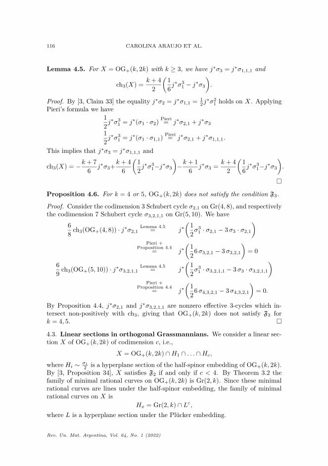
Lemma 4.5. For X = OG+(k, 2k) with k ≥ 3, we have j∗σ3 = j∗σ1,1,1 and

ch3(X) = k + 42

(16j∗σ3

1 − j∗σ3

).

Proof. By [3, Claim 33] the equality j∗σ2 = j∗σ1,1 = 12j∗σ2

1 holds on X. ApplyingPieri’s formula we have

12j∗σ3

1 = j∗(σ1 · σ2) Pieri= j∗σ2,1 + j∗σ3

12j∗σ3

1 = j∗(σ1 · σ1,1) Pieri= j∗σ2,1 + j∗σ1,1,1.

This implies that j∗σ3 = j∗σ1,1,1 and

ch3(X) = −k + 76 j∗σ3+k + 4

6

(12j∗σ3

1−j∗σ3

)−k + 1

6 j∗σ3 = k + 42

(16j∗σ3

1−j∗σ3

).

�

Proposition 4.6. For k = 4 or 5, OG+(k, 2k) does not satisfy the condition F3.

Proof. Consider the codimension 3 Schubert cycle σ2,1 on Gr(4, 8), and respectivelythe codimension 7 Schubert cycle σ3,2,1,1 on Gr(5, 10). We have

68 ch3(OG+(4, 8)) · j∗σ2,1

Lemma 4.5= j∗(

12σ

31 · σ2,1 − 3σ3 · σ2,1

)Pieri +

Proposition 4.4= j∗(

126σ3,2,1 − 3σ3,2,1

)= 0

69 ch3(OG+(5, 10)) · j∗σ3,2,1,1

Lemma 4.5= j∗(

12σ

31 · σ3,2,1,1 − 3σ3 · σ3,2,1,1

)Pieri +

Proposition 4.4= j∗(

126σ4,3,2,1 − 3σ4,3,2,1

)= 0.

By Proposition 4.4, j∗σ2,1 and j∗σ3,2,1,1 are nonzero effective 3-cycles which in-tersect non-positively with ch3, giving that OG+(k, 2k) does not satisfy F3 fork = 4, 5. �

4.3. Linear sections in orthogonal Grassmannians. We consider a linear sec-tion X of OG+(k, 2k) of codimension c, i.e.,

X = OG+(k, 2k) ∩H1 ∩ . . . ∩Hc,

where Hi ∼ σ12 is a hyperplane section of the half-spinor embedding of OG+(k, 2k).

By [3, Proposition 34], X satisfies F2 if and only if c < 4. By Theorem 3.2 thefamily of minimal rational curves on OG+(k, 2k) is Gr(2, k). Since these minimalrational curves are lines under the half-spinor embedding, the family of minimalrational curves on X is

Hx = Gr(2, k) ∩ Lc,where L is a hyperplane section under the Plucker embedding.



Proposition 4.7. For k = 5 and c < 4, OG+(5, 10) ∩ Hc does not satisfy thecondition F3.

Proof. This follows from Theorem 2.1 as Hx = Gr(2, 5)∩Lc does not satisfy F2 by[3, Proposition 32 (iv)]. �

4.4. Type C: symplectic Grassmannian.

Proposition 4.8. For 2 ≤ k < n2 , SG(k, n) does not satisfy the condition F3.

Proof. Let X = SG(k, n). By Theorem 2.1 X does not satisfy F3 as ρ(Hx) > 1. �

Now we consider SG(k, 2k) and show that in fact this also fails to satisfy thecondition F3. First, we consider the following result by Coskun.

Proposition 4.9 ([9, Corollary 3.38]). Let i : SG(k, 2k) ↪→ Gr(k, 2k) be the naturalinclusion, and σλ1,...,λj

a Schubert cycle in Gr(k, 2k). Then i∗σλ1,...,λj= 0 unless

k + 1− j ≥ λj for all j with 1 ≤ j ≤ k.

Corollary 4.10. i∗σk,k−1,...,2,1 6= 0.

Proof. By Proposition 4.9, the condition for a Schubert cycle to be nonzero onSG(k, 2k) is that k ≥ λ1, k−1 ≥ λ2, . . . , 2 ≥ λk−1, 1 ≥ λk. Therefore the only codi-mension k(k+1)

2 Schubert cycle whose restriction could be nonzero is σk,k−1,...,2,1.By non-degeneracy of the intersection pairing in cohomology on Gr(k, 2k), we havenecessarily that i∗σk,k−1,...,2,1 6= 0. �

We recall from [3, §6.3] the expression of the third Chern character in terms ofrestrictions of Schubert cycles from Gr(k, 2k):

ch3(SG(k, 2k)) = −k + 16 i∗σ3 −

−k + 46 i∗σ2,1 + −k + 7

6 i∗σ1,1,1.

Lemma 4.11. For X = SG(k, 2k) with k ≥ 3, we have i∗σ3 = i∗σ1,1,1 and

ch3(X) = −k + 42 i∗

(σ3 −

16σ

31

).

Proof. By [3, Claim 35] the equality i∗σ2 = i∗σ1,1 = i∗ 12σ

21 holds on X. Applying

Pieri’s formula we have12 i∗σ3

1 = i∗(σ1 · σ2) Pieri= i∗σ2,1 + i∗σ3

12 i∗σ3

1 = i∗(σ1 · σ1,1) Pieri= i∗σ2,1 + i∗σ1,1,1.

This implies that i∗σ3 = i∗σ1,1,1 and

ch3(X) = −k + 16 i∗σ3−

−k + 46 i∗

(12σ

31−σ3

)+−k + 7

6 i∗σ3 = −k + 42 i∗

(σ3−

16σ

31

).

�



Proposition 4.12. SG(k, 2k) does not satisfy the condition F3.

Proof. We consider the cycle ρ := σk−1,k−2,k−3,k−3,k−4,...,2,1 on Gr(k, 2k): it hascodimension k(k+1)

2 − 3 and its restriction i∗ρ to SG(k, 2k) is effective as it is anon-negative linear combination of effective cycles on SG(k, 2k) by [37, §1]. By thePieri rule and Proposition 4.9 we have

i∗(σ3 · ρ) = i∗σk,k−1,...,2,1, i∗(σ31 · ρ) = 6 · i∗σk,k−1,...,2,1.

It follows that i∗ρ 6= 0 as i∗σk,k−1,...,2,1 6= 0 by Corollary 4.10, and

ch3(SG(k, 2k)) · i∗ρ Lemma 4.11= −k + 42

(σ3 −

16σ

31

)· i∗ρ

= −k + 42 i∗

(σk,k−1,...,2,1 −

166 · σk,k−1,...,2,1

)= 0.

Therefore SG(k, 2k) does not satisfy F3. �

5. Rational homogeneous varieties of exceptional type

In this section, we show that none of the exceptional groups, when quotientedby a maximal parabolic subgroup, satisfies the condition F3, and we study whenthe condition F2 is satisfied. We recall the Dynkin diagrams of exceptional typeand mark in black the short roots, i.e., the roots such that there is an arrow in thediagram pointing in their direction.

E6 E7 E8 F4 G2

1

2

3 4 5 6 1

2

3 4 5 6 7 1

2

3 4 5 6 7 8 1 2 3 4 12

Proposition 5.1. En/Pα with α 6= 1, 2, n and F4/P2 do not satisfy F2.

Proof. Let X be one of the homogeneous spaces in the statement. By Theorem 3.2,Hx is a product and thus has Picard rank > 1. To show that X does not satisfyF2, we check that the polarized variety (Hx, Lx) is not isomorphic to any of theexceptional pairs (a)–(e) from the list in Theorem 2.3:

- For X = En/Pα and α = 3, 5, we have Hx

∼= Gr(2, k) × Pl, for somek = 5, 6, 7 and l = 1, 2, 3.

- For X = En/P4, we have Hx

∼= P2 × P1 × Pn−4.- For X = En/P

6, n = 7, 8, we have Hx∼= D5/P

5 × Pn−6 ∼= OG+(5, 10) ×Pn−6.

- For X = E8/P7, we have Hx

∼= E6/P6 × P1.

- For X = F4/P2, we have Hx

∼= P1 × P2. By Theorem 3.2, the embeddingof Hx in P(TxX) is not minimal, and thus Lx 6= O(1, 1).

Thus, X does not satisfy F2. �



5.1. Type E.

5.1.1. Parabolic groups P 1, P 2.

Proposition 5.2. En/P 1 satisfies the condition F2 but not F3 for n = 6, 7, 8.

Proof. Let X = En/P1. By Theorem 3.2 we have that Hx = Dn−1/P

n−1 =OG+(n− 1, 2(n− 1)) and Lx is a generator of Pic(Hx). Write k = n− 1. We haved = dim(Hx) = k(k−1)

2 and σ12 ∼ Lx, as Pic(Hx) = Z[σ1

2 ], where we denote by thesame symbol the Schubert cycle σ1 in Gr(k, 2k) and its restriction to OG+(k, 2k).

As b4(X) = 1 by Lemma 3.1, we apply Theorem 2.3 and conclude that X satisfiesF2 as

−2KHx − dLx = 2 · 2(k − 1)Lx −k(k − 1)

2 Lx = (k − 1)(8− k)2 Lx

is ample. We compute

T (ch3(X)) (2.2)= ch2(Hx)− 12

(c1(Hx)− d

2 c1(Lx))Lx −

d− 412 L2

x

= 2L2x −

12

(2(k − 1)− k(k − 1)

4

)L2x −

k(k − 1)− 824 L2

x

= (k − 5)(k − 8)12 L2

x,

which implies that ch3(X) is not positive, so X does not satisfy F3. �

Remark 5.3. As E6/P6 ∼= E6/P

1, Proposition 5.2 holds for E6/P6 as well.

Proposition 5.4. En/P 2 satisfies the condition F2 but not F3 for n = 6, 7, 8.

Proof. Let X = En/P2. By Theorem 3.2 we have Hx = An−1/P

3 = Gr(3, n) andLx is a generator of Pic(Hx), therefore d = dim(Hx) = 3(n− 3) and σ1 ∼ Lx. Asb4(X) = 1 by Lemma 3.1, we apply Theorem 2.3 and conclude that X satisfies F2as −2KHx − dLx = 2nLx − 3(n− 3)Lx = (9− n)Lx is ample.

For n = 8, Hx does not satisfy F2, hence X does not satisfy F3 by Theorem 2.1.From now on we assume that n = 6, 7. We have

T (ch3(X)) (2.2)= ch2(Hx)− 12

(c1(Hx)− d

2 c1(Lx))Lx −

d− 412 L2

x

= n− 42 σ2 −

n− 82 σ1,1 −

12

(n− 3(n− 3)

2

)σ2

1 −3n− 13

12 σ21

Pieri=(n− 4

2 − n

2 + 3(n− 3)4 − 3n− 13

12

)σ2

1 −(n− 8

2 + n− 42

)σ1,1

= −19 + 3n6 σ2

1 − (n− 6)σ1,1.

If n = 6 we have T (ch3(X)) < 0, and if n = 7 we have T (ch3(X)) · σ4,3,3 =− 2

3 < 0. In both cases, this implies that ch3(X) is not positive, hence X does notsatisfy F3. �



5.1.2. Freudenthal variety. The homogeneous variety E7/P7 is also known as the

Freudenthal variety G(O3,O6); it has dimension 27 and index 18. We refer forinstance to [7, §2.1 and §2.3] for more details on the geometry of E7/P

7.

Proposition 5.5. E7/P7 satisfies the condition F2 but not F3.

Proof. Let X = E7/P7. By Theorem 3.2 we have Hx = E6/P

6 and Lx is agenerator of Pic(Hx), therefore d = dim(Hx) = 16 and Lx ∼ H, as the hyperplanesection H in Hx is a generator of Pic(Hx) by [22, Proposition 5.1]. By Lemma 3.1b4(X) = 1, hence we apply Theorem 2.3 and obtain that X satisfies F2 as

2T (ch2(Hx)) = −2KHx− dLx = 24H − 16H = 8H

is ample. We apply Eq. (2.1) to compute:

T (ch3(X)) (2.2)= ch2(Hx)− 12

(c1(Hx)− d

2 c1(Lx))· Lx −

d− 412 L2

x

Lemma 5.6= 3H2 − 124H2 −H2 = 0.

We conclude that X does not satisfy F3. �

Lemma 5.6. ch2(E6/P6) = 3H2 and ch3(E6/P

6) = 0.

Proof. Let X = E6/P1 = E6/P

6; as described for instance in [22], X admits anembedding in P26. Denote by N the normal bundle of X in PV ∼= P26; by [22,Proposition 7.1] we have c1(N ) = 15H, c2(N ) = 102H2, and c3(N ) = 414H3,where H denotes a hyperplane section. Then we obtain

ch2(X) = ch2(P26)|X − ch2(N ) = 3H2,

ch3(X) = ch3(P26)|X − ch3(N ) = 0. �

Proposition 5.7. E8/P8 satisfies the condition F2 but not F3.

Proof. Let X = E8/P8. By Theorem 3.2 we have H1 := Hx = E7/P

7 the Freuden-thal variety, whose corresponding minimal family of rational curves through a gen-eral point is H2 = E6/P

6. Thus, we have d = dim(H1) = 27, c1(H1) = 18L1and by [7, §2.3] Pic(Hi) = Z[hi], where hi denotes a hyperplane class on Hi; byTheorem 3.2, hi ∼ Li.

We have b4(X) = 1 by Lemma 3.1; hence we apply Theorem 2.3 and obtain thatX satisfies F2 as −2KH1 − dL1 = 36L1 − 27L1 = 9L1 is ample. We compute

T (ch3(X)) (2.2)= ch2(H1)− 12

(c1(H1)− d

2 c1(L1))L1 −

d− 412 L2

1

= ch2(H1)− 94L

21 −

2312L

21 = ch2(H1)− 25

6 L21

T ◦ T (ch3(X)) = T (ch2(H1))− 256 T (L2

1) Prop 5.5= 4L2 −256 T (L2

1)

≤ 4L2 −256 L2 = −1

6L2,



where the last inequality holds by [2, Lemma 2.7 (1)]. We conclude that X doesnot satisfy F3. �

5.2. Type F.

Proposition 5.8. F4/P1 does not satisfy the condition F2.

Proof. Let X = F4/P1. By Theorem 3.2 we have Hx = C3/P

3 = SG(3, 6), and theembedding of Hx in P(TxX) is not minimal. Therefore Pic(Hx) is not generatedby [Lx]. Since this pair (Hx, Lx) is not in the exceptional list of Theorem 2.3, weconclude that X does not satisfy F2. �

Proposition 5.9. F4/P3 does not satisfy the condition F2.

Proof. Let X = F4/P3. By [27, Proposition 6.9] Hx is a nontrivial Q4-bundle over

P1, in particular ρ(Hx) 6= 1. Note that none of the exceptional pairs (Hx, Lx) inTheorem 2.3 admit a nontrivial Q4-fibration. We conclude that X does not satisfyF2. �

Proposition 5.10. F4/P4 satisfies the condition F2 but not F3.

Proof. By [27, proof of Proposition 6.5] F4/P4 is the generic hyperplane section of

E6/P6. We write X = E6/P

6 ∩ H, Y = E6/P6 and recall that Pic(X) = Z[H].

From Lemma 5.6 and Eq. (6.1), we obtain

ch2(X) =(

ch2(Y )− 12H

2)|Y

=(

3H2 − 12H

2)|Y

= 52H

2|x

ch3(X) =(

ch3(Y )− 16H

3)|Y

= −16H

3|X .

This implies that X = F4/P4 satisfies F2 but not F3. �

5.3. Type G.

Proposition 5.11. G2/P1 satisfies the condition F2 but not F3.

Proof. By [27, §6.1], we have that G2/P1 = Q5 ⊂ P6. Applying Theorem 6.1 and

Eq. (6.1), we conclude that G2/P1 satisfies F2 but not F3. �

Proposition 5.12. G2/P2 satisfies the condition F2 but not F3.

Proof. Let X = G2/P2. Then X satisfies F2 by Theorem 6.1. Moreover, we have

6 · ch3(X) · c21 = (c31 − 3 c1 c2 + 3 c3) · c21 = c51 − 3 c31 c2 + 3 c3 c21= 4374− 3 · 2106 + 3 · 594 = −162,

where the Chern numbers are computed in [26, Table 1]. As c21

27 is an integral classby [26, §2], we obtain ch3(X) · c

21

27 = −1, so that X does not satisfy F3. �



6. Higher Fano manifolds with high index

In [3] Araujo and Castravet classify 2-Fano manifolds of high index. We notethat there are inaccuracies in the dimension bounds in the original statement of [3,Theorem 3]. We state their classification with the correct bounds.

Theorem 6.1 ([3, Theorem 3]). Let X be a Fano manifold of dimension n ≥ 3 andindex iX ≥ n− 2. If X satisfies F2, then X is isomorphic to one of the following:

• Pn.• Complete intersections in projective spaces:

- Quadric hypersurfaces Qn ⊂ Pn+1 with n > 2;- Complete intersections of quadrics X2·2 ⊂ Pn+2 with n > 5;- Cubic hypersurfaces X3 ⊂ Pn+1 with n > 7;- Quartic hypersurfaces in Pn+1 with n > 14;- Complete intersections X2·3 ⊂ Pn+2 with n > 10;- Complete intersections X2·2·2 ⊂ Pn+3 with n > 8.

• Complete intersections in weighted projective spaces:- Degree 4 hypersurfaces in P(2, 1, . . . , 1) with n > 11;- Degree 6 hypersurfaces in P(3, 2, 1, . . . , 1) with n > 23;- Degree 6 hypersurfaces in P(3, 1, . . . , 1) with n > 26;- Complete intersections of two quadrics in P(2, 1, . . . , 1) with n > 2.

• Gr(2, 5).• OG+(5, 10) and its linear sections of codimension c < 4.• SG(3, 6).• G2/P

2.

We recall that by [3, Lemma 8], if Y is a smooth variety and X is a smoothcomplete intersection of divisors D1, . . . , Dc in Y , then

chk(X) =(

chk(Y )− 1k!

c∑i=1

Dki

)|X

. (6.1)

In particular, let X be a smooth complete intersection of hypersurfaces of degreesd1, . . . , dc in Pn and denote by h := c1(OPn(1)) the hyperplane class in Pn. Then

chk(X) = 1k!

((n+ 1)−

∑dki

)hk|X ,

and therefore X satisfies Fk if and only if∑dki ≤ n.

Let P(a0, . . . , an) denote the weighted projective space with gcd(a0, . . . , an) = 1,and let H be the effective generator of its class group. Let X be a completeintersection of hypersurfaces in P(a0, . . . , an) with classes d1H, . . . , dcH. Assumethat X is smooth, and contained in the smooth locus of P(a0, . . . , an). Then

chk(X) = ak0 + · · ·+ akn −∑dki

k! c1(H|X)k;

it follows that X satisfies Fk if and only if∑ci=1 d

ki <

∑nj=0 a

kj .



Proof of Theorem 1.5. The list in the theorem is obtained starting from Theo-rem 6.1 and studying the positivity of the third Chern character case by case. Forcomplete intersections we apply Eq. (6.1) and we determine sharp bounds on n.The remaining 2-Fano manifolds do not satisfy the condition F3 by Propositions 4.2,4.6, 4.7, 4.12 and 5.12. �

References[1] D. N. Akhiezer, Lie Group Actions in Complex Analysis, Aspects of Mathematics, E27,

Friedr. Vieweg & Sohn, Braunschweig, 1995. MR 1334091.[2] C. Araujo and A.-M. Castravet, Polarized minimal families of rational curves and higher

Fano manifolds, Amer. J. Math. 134 (2012), no. 1, 87–107. MR 2876140.[3] C. Araujo and A.-M. Castravet, Classification of 2-Fano manifolds with high index, in A Cel-

ebration of Algebraic Geometry, 1–36, Clay Math. Proc., 18, Amer. Math. Soc., Providence,RI, 2013. MR 3114934.

[4] I. N. Bernsteın, I. M. Gel′fand and S. I. Gel′fand, Schubert cells, and the cohomology of thespaces G/P , Uspehi Mat. Nauk 28 (1973), no. 3(171), 3–26. MR 0429933.

[5] N. Bourbaki, Elements de mathematique. Fasc. XXXIV. Groupes et algebres de Lie. ChapitreIV: Groupes de Coxeter et systemes de Tits. Chapitre V: Groupes engendres par desreflexions. Chapitre VI: Systemes de racines, Actualites Scientifiques et Industrielles, No.1337, Hermann, Paris, 1968. MR 0240238.

[6] F. Campana, Connexite rationnelle des varietes de Fano, Ann. Sci. Ecole Norm. Sup. (4) 25(1992), no. 5, 539–545. MR 1191735.

[7] P. E. Chaput, L. Manivel and N. Perrin, Quantum cohomology of minuscule homogeneousspaces, Transform. Groups 13 (2008), no. 1, 47–89. MR 2421317.

[8] I. Coskun, Restriction varieties and geometric branching rules, Adv. Math. 228 (2011), no. 4,2441–2502. MR 2836127.

[9] I. Coskun, Symplectic restriction varieties and geometric branching rules, in A Celebrationof Algebraic Geometry, 205–239, Clay Math. Proc., 18, Amer. Math. Soc., Providence, RI,2013. MR 3114942.

[10] A. J. de Jong, X. He and J. M. Starr, Families of rationally simply connected varieties oversurfaces and torsors for semisimple groups, Publ. Math. Inst. Hautes Etudes Sci. No. 114(2011), 1–85. MR 2854858.

[11] A. J. de Jong and J. M. Starr, A note on Fano manifolds whose second Chern character ispositive, https://arxiv.org/abs/math/0602644v1 [math.AG], 2006.

[12] A. J. de Jong and J. M. Starr, Low degree complete intersections are rationally simplyconnected, https://www.math.stonybrook.edu/∼jstarr/papers/nk1006g.pdf, 2006.

[13] A. J. de Jong and J. Starr, Higher Fano manifolds and rational surfaces, Duke Math. J. 139(2007), no. 1, 173–183. MR 2322679.

[14] A. Fanelli, L. Gruson and N. Perrin, Rational curves on V5 and rational simple connectedness,https://arxiv.org/abs/1901.06930 [math.AG], 2019.

[15] W. Fulton, Young Tableaux, London Mathematical Society Student Texts, 35, CambridgeUniversity Press, Cambridge, 1997. MR 1464693.

[16] W. Fulton and J. Harris, Representation Theory, Graduate Texts in Mathematics, 129,Springer-Verlag, New York, 1991. MR 1153249.

[17] T. Graber, J. Harris and J. Starr, Families of rationally connected varieties, J. Amer. Math.Soc. 16 (2003), no. 1, 57–67. MR 1937199.


https://mathscinet.ams.org/mathscinet-getitem?mr=1334091










https://arxiv.org/abs/math/0602644v1

https://www.math.stonybrook.edu/~jstarr/papers/nk1006g.pdf


https://arxiv.org/abs/1901.06930





[18] J. E. Humphreys, Introduction to Lie Algebras and Representation Theory, Graduate Textsin Mathematics, Vol. 9, Springer-Verlag, New York, 1972. MR 0323842.

[19] J. E. Humphreys, Linear Algebraic Groups, Graduate Texts in Mathematics, No. 21,Springer-Verlag, New York, 1975. MR 0396773.

[20] J.-M. Hwang, Geometry of minimal rational curves on Fano manifolds, in School on VanishingTheorems and Effective Results in Algebraic Geometry (Trieste, 2000), 335–393, ICTP Lect.Notes, 6, Abdus Salam Int. Cent. Theoret. Phys., Trieste, 2001. MR 1919462.

[21] J.-M. Hwang and N. Mok, Birationality of the tangent map for minimal rational curves,Asian J. Math. 8 (2004), no. 1, 51–63. MR 2128297.

[22] A. Iliev and L. Manivel, The Chow ring of the Cayley plane, Compos. Math. 141 (2005),no. 1, 146–160. MR 2099773.

[23] S. Kebekus, Families of singular rational curves, J. Algebraic Geom. 11 (2002), no. 2, 245–256. MR 1874114.

[24] J. Kollar, Rational curves on algebraic varieties, Ergebnisse der Mathematik und ihrer Gren-zgebiete. 3. Folge. A Series of Modern Surveys in Mathematics, 32, Springer-Verlag, Berlin,1996. MR 1440180.

[25] J. Kollar, Y. Miyaoka and S. Mori, Rational connectedness and boundedness of Fano mani-folds, J. Differential Geom. 36 (1992), no. 3, 765–779. MR 1189503.

[26] D. Kotschick and D. K. Thung, The complex geometry of two exceptional flag manifolds,Ann. Mat. Pura Appl. (4) 199 (2020), no. 6, 2227–2241. MR 4165679.

[27] J. M. Landsberg and L. Manivel, On the projective geometry of rational homogeneous vari-eties, Comment. Math. Helv. 78 (2003), no. 1, 65–100. MR 1966752.

[28] J. M. Landsberg and L. Manivel, Representation theory and projective geometry, in Alge-braic transformation groups and algebraic varieties, 71–122, Encyclopaedia Math. Sci., 132,Invariant Theory Algebr. Transform. Groups, III, Springer, Berlin, 2004. MR 2090671.

[29] S. Lang, On quasi algebraic closure, Ann. of Math. (2) 55 (1952), 373–390. MR 0046388.[30] L. Manivel, Topics on the geometry of rational homogeneous spaces, Acta Math. Sin. (Engl.

Ser.) 36 (2020), no. 8, 851–872. MR 4129512.[31] J. S. Milne, Lie Algebras, Algebraic Groups, and Lie Groups, 2013. Available at https://

www.jmilne.org/math/CourseNotes/LAG.pdf.[32] S. Mori, Projective manifolds with ample tangent bundles, Ann. of Math. (2) 110 (1979),

no. 3, 593–606. MR 0554387.[33] T. Nagaoka, On a sufficient condition for a Fano manifold to be covered by rational N -folds,

J. Pure Appl. Algebra 223 (2019), no. 11, 4677–4688. MR 3955036.[34] J. Nagel, Cohomology of quadric bundles, Habilitation thesis, Universite Lille 1, 2006. Avail-

able at http://nagel49.perso.math.cnrs.fr/habilitation.pdf.[35] B. Pasquier, Introduction to Spherical Varieties and Description of Special Classes of Spher-

ical Varieties, 2009. Available at http://www-math.sp2mi.univ-poitiers.fr/∼bpasquie/KIAS.pdf.

[36] P. Pragacz, A generalization of the Macdonald–You formula, J. Algebra 204 (1998), no. 2,573–587. MR 1624487.

[37] P. Pragacz, Addendum: “A generalization of the Macdonald–You formula”, J. Algebra 226(2000), no. 1, 639–648. MR 1749909.

[38] D. Snow, Homogeneous Vector Bundles. Available at https://www3.nd.edu/∼snow/Papers/HomogVB.pdf.

[39] T. A. Springer, Linear Algebraic Groups, second edition, Progress in Mathematics, 9,Birkhauser Boston, 1998. MR 1642713.















https://www.jmilne.org/math/CourseNotes/LAG.pdf

https://www.jmilne.org/math/CourseNotes/LAG.pdf



http://nagel49.perso.math.cnrs.fr/habilitation.pdf

http://www-math.sp2mi.univ-poitiers.fr/~bpasquie/KIAS.pdf

http://www-math.sp2mi.univ-poitiers.fr/~bpasquie/KIAS.pdf



https://www3.nd.edu/~snow/Papers/HomogVB.pdf

https://www3.nd.edu/~snow/Papers/HomogVB.pdf



[40] J. M. Starr, Hypersurfaces of low degree are rationally simply-connected, https://arxiv.org/abs/math/0602641 [math.AG], 2006.

[41] J. M. Starr, Brauer Groups and Galois Cohomology of Function Fields of Varieties, Pub-licacoes Matematicas do IMPA, Instituto Nacional de Matematica Pura e Aplicada (IMPA),Rio de Janeiro, 2008. MR 2440271.

[42] T. Suzuki, Higher order minimal families of rational curves and Fano manifolds with nefChern characters, J. Math. Soc. Japan 73 (2021), no. 3, 949–964. MR 4291439.

Carolina AraujoB

IMPA, Estrada Dona Castorina 110, 22460-320 Rio de Janeiro, [email protected]

Roya BeheshtiDepartment of Mathematics & Statistics, Washington University in St. Louis, St. Louis,MO 63130, [email protected]

Ana-Maria CastravetUniversite Paris-Saclay, UVSQ, Laboratoire de Mathematiques de Versailles, 78000, Versailles,[email protected]

Kelly JabbuschDepartment of Mathematics & Statistics, University of Michigan–Dearborn, 4901 Evergreen Rd,Dearborn, MI 48128, [email protected]

Svetlana MakarovaDepartment of Mathematics, University of Pennsylvania, 209 S 33rd St, Philadelphia, PA 19104,[email protected]

Enrica MazzonMax-Planck-Institut fur Mathematik, Vivatsgasse 7, 53111, Bonn, [email protected]

Libby TaylorStanford University, 380 Serra Mall, Stanford, CA 94305, [email protected]

Nivedita ViswanathanSchool of Mathematics, The University of Edinburgh, Edinburgh, EH9 3FD, [email protected]

Received: June 10, 2021Accepted: July 19, 2021


https://arxiv.org/abs/math/0602641

https://arxiv.org/abs/math/0602641



higher fano manifolds - INMABB

Documents

Transcript of higher fano manifolds - INMABB