8-bit optimizers via block-wise quantization - arXiv

Published as a conference paper at ICLR 2022

8-BIT OPTIMIZERS VIA BLOCK-WISE QUANTIZATION

Tim Dettmers∗‡ Mike Lewis∗ Sam Shleifer∗ Luke Zettlemoyer∗‡Facebook AI Research∗, mikelewis,[email protected] of Washington‡, dettmers,[email protected]

ABSTRACT

Stateful optimizers maintain gradient statistics over time, e.g., the exponentiallysmoothed sum (SGD with momentum) or squared sum (Adam) of past gradi-ent values. This state can be used to accelerate optimization compared to plainstochastic gradient descent but uses memory that might otherwise be allocated tomodel parameters, thereby limiting the maximum size of models trained in prac-tice. In this paper, we develop the first optimizers that use 8-bit statistics whilemaintaining the performance levels of using 32-bit optimizer states. To overcomethe resulting computational, quantization, and stability challenges, we developblock-wise dynamic quantization. Block-wise quantization divides input tensorsinto smaller blocks that are independently quantized. Each block is processed inparallel across cores, yielding faster optimization and high precision quantization.To maintain stability and performance, we combine block-wise quantization withtwo additional changes: (1) dynamic quantization, a form of non-linear optimiza-tion that is precise for both large and small magnitude values, and (2) a stable em-bedding layer to reduce gradient variance that comes from the highly non-uniformdistribution of input tokens in language models. As a result, our 8-bit optimizersmaintain 32-bit performance with a small fraction of the memory footprint ona range of tasks, including 1.5B parameter language modeling, GLUE finetun-ing, ImageNet classification, WMT’14 machine translation, MoCo v2 contrastiveImageNet pretraining+finetuning, and RoBERTa pretraining, without changes tothe original optimizer hyperparameters. We open-sourceour 8-bit optimizers as adrop-in replacement that only requires a two-line code change.

Increasing model size is an effective way to achieve better performance for given resources (Kaplanet al., 2020; Henighan et al., 2020; Raffel et al., 2019; Lewis et al., 2021). However, training suchlarge models requires storing the model, gradient, and state of the optimizer (e.g., exponentiallysmoothed sum and squared sum of previous gradients for Adam), all in a fixed amount of availablememory. Although significant research has focused on enabling larger model training by reducing orefficiently distributing the memory required for the model parameters (Shoeybi et al., 2019; Lepikhinet al., 2020; Fedus et al., 2021; Brown et al., 2020; Rajbhandari et al., 2020), reducing the memoryfootprint of optimizer gradient statistics is much less studied. This is a significant missed opportunitysince these optimizer states use 33-75% of the total memory footprint during training. For example,the Adam optimizer states for the largest GPT-2 (Radford et al., 2019) and T5 (Raffel et al., 2019)models are 11 GB and 41 GB in size. In this paper, we develop a fast, high-precision non-linearquantization method – block-wise dynamic quantization – that enables stable 8-bit optimizers (e.g.,Adam, AdamW, and Momentum) which maintain 32-bit performance at a fraction of the memoryfootprint and without any changes to the original hyperparameters.1

While most current work uses 32-bit optimizer states, recent high-profile efforts to use 16-bit opti-mizers report difficultly for large models with more than 1B parameters (Ramesh et al., 2021). Goingfrom 16-bit optimizers to 8-bit optimizers reduces the range of possible values from 216 = 65536values to just 28 = 256. To our knowledge, this has not been attempted before.

Effectively using this very limited range is challenging for three reasons: quantization accuracy,computational efficiency, and large-scale stability. To maintain accuracy, it is critical to introducesome form of non-linear quantization to reduce errors for both common small magnitude values

1We study 8-bit optimization with current best practice model and gradient representations (typically 16-bitmixed precision), to isolate optimization challenges. Future work could explore further compressing all three.

1

arX

iv:2

110.

0286

1v2

[cs

.LG

] 2

0 Ju

n 20

22

mikelewis,[email protected]

dettmers,[email protected]


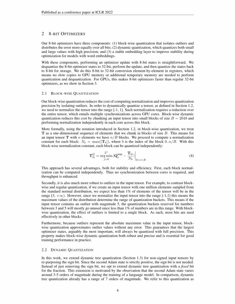
-3.1 0.1 -0.03 1.2

-1.0 0.032 -0.025 1.0

3.1 1.2

-1.0 0.0329 -0.0242 1.0

0 170 80 255

-1.0*3.1 0.0329*3.1 -0.0242*1.2 1.0*1.2

-3.1 0.102 -0.029 1.2

0 170 80 255

-1.0 0.0329 -0.0242 1.0

Quantization Dequantization

Optimizer State

Chunk into blocks

Find block-wise absmax

Normalize with absmax

Find closest 8-bit value

-3.1 0.1 -0.03 1.2

Find corresponding index

Store index values

Load Index values

Index

Lookup values

Denormalize by absmax

Dequantized optimizer states

Updated optimizer states

Update optimizer states

Figure 1: Schematic of 8-bit optimizers via block-wise dynamic quantization, see Section 2 for moredetails. After the optimizer update is performed in 32-bit, the state tensor is chunked into blocks,normalized by the absolute maximum value of each block. Then dynamic quantization is performed,and the index is stored. For dequantization, a lookup in the index is performed, with subsequent de-normalization by multiplication with the block-wise absolute maximum value. Outliers are confinedto a single block through block-wise quantization, and their effect on normalization is limited.

and rare large ones. However, to be practical, 8-bit optimizers need to be fast enough to not slowdown training, which is especially difficult for non-linear methods that require more complex datastructures to maintain the quantization buckets. Finally, to maintain stability with huge modelsbeyond 1B parameters, a quantization method needs to not only have a good mean error but excellentworse case performance since a single large quantization error can cause the entire training run todiverge.

We introduce a new block-wise quantization approach that addresses all three of these challenges.Block-wise quantization splits input tensors into blocks and performs quantization on each block in-dependently. This block-wise division reduces the effect of outliers on the quantization process sincethey are isolated to particular blocks, thereby improving stability and performance, especially forlarge-scale models. Block-wise processing also allows for high optimizer throughput since each nor-malization can be computed independently in each core. This contrasts with tensor-wide normaliza-tion, which requires slow cross-core synchronization that is highly dependent on task-core schedul-ing. We combine block-wise quantization with two novel methods for stable, high-performance 8-bitoptimizers: dynamic quantization and a stable embedding layer. Dynamic quantization is an exten-sion of dynamic tree quantization for unsigned input data. The stable embedding layer is a variationof a standard word embedding layer that supports more aggressive quantization by normalizing thehighly non-uniform distribution of inputs to avoid extreme gradient variation.

Our 8-bit optimizers maintain 32-bit performance at a fraction of the original memory footprint.We show this for a broad range of tasks: 1.5B and 355M parameter language modeling, GLUEfinetuning, ImageNet classification, WMT’14+WMT’16 machine translation, MoCo v2 contrastiveimage pretraining+finetuning, and RoBERTa pretraining. We also report additional ablations andsensitivity analysis showing that all components – block-wise quantization, dynamic quantization,and stable embedding layer – are crucial for these results and that 8-bit Adam can be used as a simpledrop-in replacement for 32-bit Adam, with no hyperparameter changes. We open-source our customCUDA kernels and provide a PyTorch implementation that enables 8-bit optimization by changingtwo lines of code.

1 BACKGROUND

1.1 STATEFUL OPTIMIZERS

An optimizer updates the parameters w of a neural network by using the gradient of the loss withrespect to the weight gt = ∂L

∂w at update iteration t. Stateful optimizers compute statistics of thegradient with respect to each parameter over time for accelerated optimization. Two of the most

2


commonly used stateful optimizers are Adam (Kingma and Ba, 2014), and SGD with momentum(Qian, 1999) – or Momentum for short. Without damping and scaling constants, the update rules ofthese optimizers are given by:

Momentum(gt,wt−1,mt−1) =

m0 = g0 Initializationmt = β1mt−1 + gt State 1 updatewt = wt−1 − α ·mt Weight update

(1)

Adam(gt,wt−1,mt−1, rt−1) =

r0 = m0 = 0 Initializationmt = β1mt−1 + (1− β1)gt State 1 updatert = β2rt−1 + (1− β2)g2

t State 2 updatewt = wt−1 − α · mt√

rt+εWeight update,

(2)

where β1 and β2 are smoothing constants, ε is a small constant, and α is the learning rate.

For 32-bit states, Momentum and Adam consume 4 and 8 bytes per parameter. That is 4 GB and 8GB for a 1B parameter model. Our 8-bit non-linear quantization reduces these costs to 1 GB and 2GB.

1.2 NON-LINEAR QUANTIZATION

Quantization compresses numeric representations to save space at the cost of precision. Quanti-zation is the mapping of a k-bit integer to a real element in D, that is, Qmap : [0, 2k − 1] 7→ D.For example, the IEEE 32-bit floating point data type maps the indices 0...232 − 1 to the do-main [-3.4e38, +3.4e38]. We use the following notation: Qmap(i) = Qmap

i = qi, for exampleQmap(231 + 131072) = 2.03125, for the IEEE 32-bit floating point data type.

To perform general quantization from one data type into another we require three steps. (1) Computea normalization constant N that transforms the input tensor T into the range of the domain D of thetarget quantization data type Qmap, (2) for each element of T/N find the closest corresponding valueqi in the domain D, (3) store the index i corresponding to qi in the quantized output tensor TQ. Toreceive the dequantized tensor TD we look up the index and denormalize: TD

i = Qmap(TQi ) ·N .

To perform this procedure for dynamic quantization we first normalize into the range [-1, 1] throughdivision by the absolute maximum value: N = max(|T|).Then we find the closest values via a binary search:

TQi =

2n

argminj=0

|Qmapj − Ti

N| (3)

1.3 DYNAMIC TREE QUANTIZATION

Figure 2: Dynamic tree quantization.

Dynamic Tree quantization (Dettmers, 2016) is a methodthat yields low quantization error for both small and largemagnitude values. Unlike data types with fixed exponentand fraction, dynamic tree quantization uses a datatypewith a dynamic exponent and fraction that can changewith each number. It is made up of four parts, as seen inFigure 2: (1) The first bit of the data type is reserved fora sign. (2) The number of subsequent zero bits indicatesthe magnitude of the exponent. (3) The first bit that is setto one indicates that all following values are reserved for(4) linear quantization. By moving the indicator bit, num-bers can have a large exponent 10−7 or precision as high as 1/63. Compared to linear quantization,dynamic tree quantization has better absolute and relative quantization errors for non-uniform dis-tributions. Dynamic tree quantization is strictly defined to quantize numbers in the range [-1.0, 1.0],which is ensured by performing tensor-level absolute max normalization.

3


2 8-BIT OPTIMIZERS

Our 8-bit optimizers have three components: (1) block-wise quantization that isolates outliers anddistributes the error more equally over all bits; (2) dynamic quantization, which quantizes both smalland large values with high precision; and (3) a stable embedding layer to improve stability duringoptimization for models with word embeddings.

With these components, performing an optimizer update with 8-bit states is straightforward. Wedequantize the 8-bit optimizer states to 32-bit, perform the update, and then quantize the states backto 8-bit for storage. We do this 8-bit to 32-bit conversion element-by-element in registers, whichmeans no slow copies to GPU memory or additional temporary memory are needed to performquantization and dequantization. For GPUs, this makes 8-bit optimizers faster than regular 32-bitoptimizers, as we show in Section 3.

2.1 BLOCK-WISE QUANTIZATION

Our block-wise quantization reduces the cost of computing normalization and improves quantizationprecision by isolating outliers. In order to dynamically quantize a tensor, as defined in Section 1.2,we need to normalize the tensor into the range [-1, 1]. Such normalization requires a reduction overthe entire tensor, which entails multiple synchronizations across GPU cores. Block-wise dynamicquantization reduces this cost by chunking an input tensor into small blocks of size B = 2048 andperforming normalization independently in each core across this block.

More formally, using the notation introduced in Section 1.2, in block-wise quantization, we treatT as a one-dimensional sequence of elements that we chunk in blocks of size B. This means foran input tensor T with n elements we have n/B blocks. We proceed to compute a normalizationconstant for each block: Nb = max(|Tb|), where b is the index of the block 0..n/B. With thisblock-wise normalization constant, each block can be quantized independently:

TQbi =

2n

argminj=0

|Qmapj − Tbi

Nb|∣∣∣∣0<i<B

(4)

This approach has several advantages, both for stability and efficiency. First, each block normal-ization can be computed independently. Thus no synchronization between cores is required, andthroughput is enhanced.

Secondly, it is also much more robust to outliers in the input tensor. For example, to contrast block-wise and regular quantization, if we create an input tensor with one million elements sampled fromthe standard normal distribution, we expect less than 1% of elements of the tensor will be in therange [3, +∞). However, since we normalize the input tensor into the range [-1,1] this means themaximum values of the distribution determine the range of quantization buckets. This means if theinput tensor contains an outlier with magnitude 5, the quantization buckets reserved for numbersbetween 3 and 5 will mostly go unused since less than 1% of numbers are in this range. With block-wise quantization, the effect of outliers is limited to a single block. As such, most bits are usedeffectively in other blocks.

Furthermore, because outliers represent the absolute maximum value in the input tensor, block-wise quantization approximates outlier values without any error. This guarantees that the largestoptimizer states, arguably the most important, will always be quantized with full precision. Thisproperty makes block-wise dynamic quantization both robust and precise and is essential for goodtraining performance in practice.

2.2 DYNAMIC QUANTIZATION

In this work, we extend dynamic tree quantization (Section 1.3) for non-signed input tensors byre-purposing the sign bit. Since the second Adam state is strictly positive, the sign bit is not needed.Instead of just removing the sign bit, we opt to extend dynamic tree quantization with a fixed bitfor the fraction. This extension is motivated by the observation that the second Adam state variesaround 3-5 orders of magnitude during the training of a language model. In comparison, dynamictree quantization already has a range of 7 orders of magnitude. We refer to this quantization as

4


dynamic quantization to distinguish it from dynamic tree quantization in our experiments. A studyof additional quantization data types and their performance is detailed in Appendix F.

2.3 STABLE EMBEDDING LAYER

Our stable embedding layer is a standard word embedding layer variation (Devlin et al., 2019)designed to ensure stable training for NLP tasks. This embedding layer supports more aggressivequantization by normalizing the highly non-uniform distribution of inputs to avoid extreme gradientvariation. See Appendix C for a discussion of why commonly adopted embedding layers (Ott et al.,2019) are so unstable.

We initialize the Stable Embedding Layer with Xavier uniform initialization (Glorot and Bengio,2010) and apply layer normalization (Ba et al., 2016) before adding position embeddings. Thismethod maintains a variance of roughly one both at initialization and during training. Additionally,the uniform distribution initialization has less extreme values than a normal distribution, reducingmaximum gradient size. Like Ramesh et al. (2021), we find that the stability of training improvessignificantly if we use 32-bit optimizer states for the embedding layers. This is the only layer thatuses 32-bit optimizer states. We still use the standard precision for weights and gradients for theembedding layers – usually 16-bit. We show in our Ablation Analysis in Section 4 that the StableEmbedding Layer is required for stable training. See ablations for the Xavier initialization, layernorm, and 32-bit state components of the Stable Embedding Layer in Appendix I.

3 8-BIT VS 32-BIT OPTIMIZER PERFORMANCE FOR COMMON BENCHMARKS

Experimental Setup We compare the performance of 8-bit optimizers to their 32-bit counterpartson a range of challenging public benchmarks. These benchmarks either use Adam (Kingma and Ba,2014), AdamW (Loshchilov and Hutter, 2018), or Momentum (Qian, 1999).

We do not change any hyperparameters or precision of weights, gradients, and activations/input gra-dients for each experimental setting compared to the public baseline– the only change is to replace32-bit optimizers with 8-bit optimizers. This means that for most experiments, we train in 16-bitmixed-precision (Micikevicius et al., 2017). We also compare with Adafactor (Shazeer and Stern,2018), with the time-independent formulation for β2 (Shazeer and Stern, 2018) – which is the sameformulation used in Adam. We also do not change any hyperparameters for Adafactor.

We report on benchmarks in neural machine translation (Ott et al., 2018)2 trained on WMT’16(Sennrich et al., 2016) and evaluated on en-de WMT’14 (Machacek and Bojar, 2014), large-scalelanguage modeling (Lewis et al., 2021; Brown et al., 2020) and RoBERTa pretraining (Liu et al.,2019) on English CC-100 + RoBERTa corpus (Nagel, 2016; Gokaslan and Cohen, 2019; Zhu et al.,2015; Wenzek et al., 2020), finetuning the pretrained masked language model RoBERTa (Liu et al.,2019)3 on GLUE (Wang et al., 2018a), ResNet-50 v1.5 image classification (He et al., 2016)4 onImageNet-1k (Deng et al., 2009), and Moco v2 contrastive image pretraining and linear finetuning(Chen et al., 2020b)5 on ImageNet-1k (Deng et al., 2009).

We use the stable embedding layer for all NLP tasks except for finetuning on GLUE. Beyond this, wefollow the exact experimental setup outlined in the referenced papers and codebases. We consistentlyreport replication results for each benchmark with public codebases and report median accuracy,perplexity, or BLEU over ten random seeds for GLUE, three random seeds for others tasks, anda single random seed for large scale language modeling. While it is standard to report means andstandard errors on some tasks, others use median performance. We opted to report medians for alltasks for consistency.

Results In Table 1, we see that 8-bit optimizers match replicated 32-bit performance for all tasks.While Adafactor is competitive with 8-bit Adam, 8-bit Adam uses less memory and provides fasteroptimization. Our 8-bit optimizers save up to 8.5 GB of GPU memory for our largest 1.5B pa-

2https://github.com/pytorch/fairseq/tiny/master/examples/scaling_nmt/README.md

3https://github.com/pytorch/fairseq/blob/master/examples/roberta/README.glue.md

4https://github.com/NVIDIA/DeepLearningExamples/tree/master/PyTorch/Classification/ConvNets/

5https://github.com/facebookresearch/moco

5

https://github.com/pytorch/fairseq/tiny/master/examples/scaling_nmt/README.md

https://github.com/pytorch/fairseq/blob/master/examples/roberta/README.glue.md

https://github.com/NVIDIA/DeepLearningExamples/tree/master/PyTorch/Classification/ConvNets/

https://github.com/facebookresearch/moco


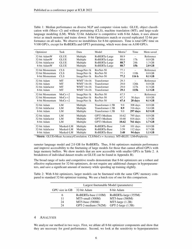
Table 1: Median performance on diverse NLP and computer vision tasks: GLUE, object classifi-cation with (Moco v2) and without pretraining (CLS), machine translation (MT), and large-scalelanguage modeling (LM). While 32-bit Adafactor is competitive with 8-bit Adam, it uses almosttwice as much memory and trains slower. 8-bit Optimizers match or exceed replicated 32-bit per-formance on all tasks. We observe no instabilities for 8-bit optimizers. Time is total GPU time onV100 GPUs, except for RoBERTa and GPT3 pretraining, which were done on A100 GPUs.

Optimizer Task Data Model Metric† Time Mem saved

32-bit AdamW GLUE Multiple RoBERTa-Large 88.9 – Reference32-bit AdamW GLUE Multiple RoBERTa-Large 88.6 17h 0.0 GB32-bit Adafactor GLUE Multiple RoBERTa-Large 88.7 24h 1.3 GB8-bit AdamW GLUE Multiple RoBERTa-Large 88.7 15h 2.0 GB

32-bit Momentum CLS ImageNet-1k ResNet-50 77.1 – Reference32-bit Momentum CLS ImageNet-1k ResNet-50 77.1 118h 0.0 GB8-bit Momentum CLS ImageNet-1k ResNet-50 77.2 116 h 0.1 GB

32-bit Adam MT WMT’14+16 Transformer 29.3 – Reference32-bit Adam MT WMT’14+16 Transformer 29.0 126h 0.0 GB32-bit Adafactor MT WMT’14+16 Transformer 29.0 127h 0.3 GB8-bit Adam MT WMT’14+16 Transformer 29.1 115h 1.1 GB

32-bit Momentum MoCo v2 ImageNet-1k ResNet-50 67.5 – Reference32-bit Momentum MoCo v2 ImageNet-1k ResNet-50 67.3 30 days 0.0 GB8-bit Momentum MoCo v2 ImageNet-1k ResNet-50 67.4 28 days 0.1 GB

32-bit Adam LM Multiple Transformer-1.5B 9.0 308 days 0.0 GB32-bit Adafactor LM Multiple Transformer-1.5B 8.9 316 days 5.6 GB8-bit Adam LM Multiple Transformer-1.5B 9.0 297 days 8.5 GB

32-bit Adam LM Multiple GPT3-Medium 10.62 795 days 0.0 GB32-bit Adafactor LM Multiple GPT3-Medium 10.68 816 days 1.5 GB8-bit Adam LM Multiple GPT3-Medium 10.62 761 days 1.7 GB

32-bit Adam Masked-LM Multiple RoBERTa-Base 3.49 101 days 0.0 GB32-bit Adafactor Masked-LM Multiple RoBERTa-Base 3.59 112 days 0.7 GB8-bit Adam Masked-LM Multiple RoBERTa-Base 3.48 94 days 1.1 GB†Metric: GLUE=Mean Accuracy/Correlation. CLS/MoCo = Accuracy. MT=BLEU. LM=Perplexity.

rameter language model and 2.0 GB for RoBERTa. Thus, 8-bit optimizers maintain performanceand improve accessibility to the finetuning of large models for those that cannot afford GPUs withlarge memory buffers. We show models that are now accessible with smaller GPUs in Table 2. Abreakdown of individual dataset results on GLUE can be found in Appendix B).

The broad range of tasks and competitive results demonstrate that 8-bit optimizers are a robust andeffective replacement for 32-bit optimizers, do not require any additional changes in hyperparame-ters, and save a significant amount of memory while speeding up training slightly.

Table 2: With 8-bit optimizers, larger models can be finetuned with the same GPU memory com-pared to standard 32-bit optimizer training. We use a batch size of one for this comparison.

Largest finetunable Model (parameters)

GPU size in GB 32-bit Adam 8-bit Adam

6 RoBERTa-base (110M) RoBERTa-large (355M)11 MT5-small (300M) MT5-base (580M)24 MT5-base (580M) MT5-large (1.2B)24 GPT-2-medium (762M) GPT-2-large (1.5B)

4 ANALYSIS

We analyze our method in two ways. First, we ablate all 8-bit optimizer components and show thatthey are necessary for good performance. Second, we look at the sensitivity to hyperparameters

6


compared to 32-bit Adam and show that 8-bit Adam with block-wise dynamic quantization is areliable replacement that does not require further hyperparameter tuning.

Experimental Setup We perform our analysis on a strong 32-bit Adam baseline for languagemodeling with transformers (Vaswani et al., 2017). We subsample from the RoBERTa corpus (Liuet al., 2019) which consists of the English sub-datasets: Books (Zhu et al., 2015), Stories (Trinh andLe, 2018), OpenWebText-1 (Gokaslan and Cohen, 2019), Wikipedia, and CC-News (Nagel, 2016).We use a 50k token BPE encoded vocabulary (Sennrich et al., 2015). We find the best 2-GPU-daytransformer baseline for 32-bit Adam with multiple hyperparameter searches that take in a totalof 440 GPU days. Key hyperparameters include 10 layers with a model dimension of 1024, a fullyconnected hidden dimension of 8192, 16 heads, and input sub-sequences with a length of 512 tokenseach. The final model has 209m parameters.

Table 3: Ablation analysis of 8-bit Adam for small (2 GPU days) and large-scale (≈1 GPU year)transformer language models on the RoBERTa corpus. The runs without dynamic quantization uselinear quantization. The percentage of unstable runs indicates either divergence or crashed trainingdue to exploding gradients. We report median perplexity for successful runs. We can see thatdynamic quantization is critical for general stability and block-wise quantization is critical for large-scale stability. The stable embedding layer is useful for both 8-bit and 32-bit Adam and enhancesstability to some degree.

Parameters Optimizer Dynamic Block-wise Stable Emb Unstable (%) Perplexity

209M

32-bit Adam 0 16.732-bit Adam X 0 16.38-bit Adam 90 253.08-bit Adam X 50 194.48-bit Adam X 10 18.68-bit Adam X X 0 17.78-bit Adam X X 0 16.88-bit Adam X X X 0 16.4

1.3B 32-bit Adam 0 10.41.3B 8-bit Adam X 100 N/A1.3B 8-bit Adam X X 80 10.9

1.5B 32-bit Adam 0 9.01.5B 8-bit Adam X X X 0 9.0

Ablation Analysis For the ablation analysis, we compare small and large-scale language model-ing perplexity and training stability against a 32-bit Adam baseline. We ablate components individ-ually and include combinations of methods that highlight their interactions. The baseline methoduses linear quantization, and we add dynamic quantization, block-wise quantization, and the stableembedding layer to demonstrate their effect. To test optimization stability for small-scale languagemodeling, we run each setting with different hyperparameters and report median performance acrossall successful runs. A successful run is a run that does not crash due to exploding gradients or di-verges in the loss. We use the hyperparameters ε 1e-8, 1e-7, 1e-6, β1 0.90, 0.87, 0.93, β20.999, 0.99, 0.98 and small changes in learning rates. We also include some partial ablations forlarge-scale models beyond 1B parameters. In the large-scale setting, we run several seeds with thesame hyperparameters. We use a single seed for 32-bit Adam, five seeds for 8-bit Adam at 1.3Bparameters, and a single seed for 8-bit Adam at 1.5B parameters.6 Results are shown in Table 3.

The Ablations show that dynamic quantization, block-wise quantization, and the stable embeddinglayer are critical for either performance or stability. In addition, block-wise quantization is criticalfor large-scale language model stability.

Sensitivity Analysis We compare the perplexity of 32-bit Adam vs 8-bit Adam + Stable Embed-ding as we change the optimizer hyperparameters: learning rate, betas, and ε. We change each hyper-parameter individually from the baseline hyperparameters β1=0.9, β2=0.995, ε=1e-7, and lr=0.0163

6We chose not to do the full ablations with such large models because each training run takes one GPU year.

7


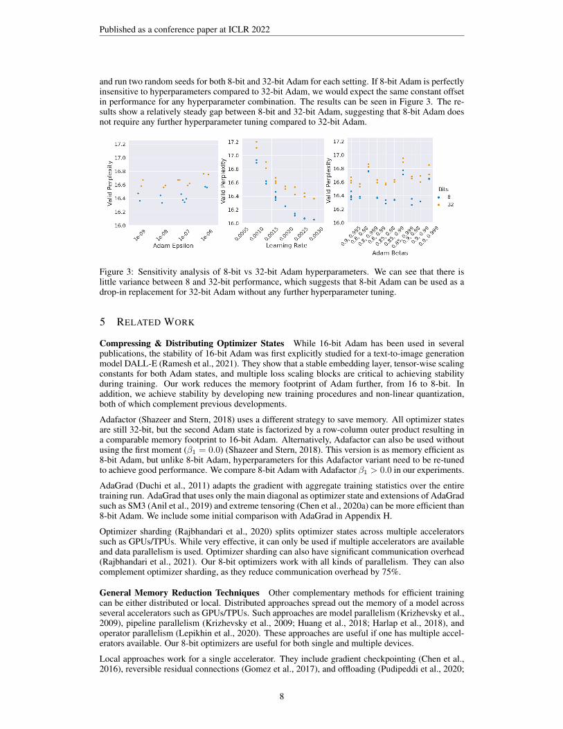
and run two random seeds for both 8-bit and 32-bit Adam for each setting. If 8-bit Adam is perfectlyinsensitive to hyperparameters compared to 32-bit Adam, we would expect the same constant offsetin performance for any hyperparameter combination. The results can be seen in Figure 3. The re-sults show a relatively steady gap between 8-bit and 32-bit Adam, suggesting that 8-bit Adam doesnot require any further hyperparameter tuning compared to 32-bit Adam.

Figure 3: Sensitivity analysis of 8-bit vs 32-bit Adam hyperparameters. We can see that there islittle variance between 8 and 32-bit performance, which suggests that 8-bit Adam can be used as adrop-in replacement for 32-bit Adam without any further hyperparameter tuning.

5 RELATED WORK

Compressing & Distributing Optimizer States While 16-bit Adam has been used in severalpublications, the stability of 16-bit Adam was first explicitly studied for a text-to-image generationmodel DALL-E (Ramesh et al., 2021). They show that a stable embedding layer, tensor-wise scalingconstants for both Adam states, and multiple loss scaling blocks are critical to achieving stabilityduring training. Our work reduces the memory footprint of Adam further, from 16 to 8-bit. Inaddition, we achieve stability by developing new training procedures and non-linear quantization,both of which complement previous developments.

Adafactor (Shazeer and Stern, 2018) uses a different strategy to save memory. All optimizer statesare still 32-bit, but the second Adam state is factorized by a row-column outer product resulting ina comparable memory footprint to 16-bit Adam. Alternatively, Adafactor can also be used withoutusing the first moment (β1 = 0.0) (Shazeer and Stern, 2018). This version is as memory efficient as8-bit Adam, but unlike 8-bit Adam, hyperparameters for this Adafactor variant need to be re-tunedto achieve good performance. We compare 8-bit Adam with Adafactor β1 > 0.0 in our experiments.

AdaGrad (Duchi et al., 2011) adapts the gradient with aggregate training statistics over the entiretraining run. AdaGrad that uses only the main diagonal as optimizer state and extensions of AdaGradsuch as SM3 (Anil et al., 2019) and extreme tensoring (Chen et al., 2020a) can be more efficient than8-bit Adam. We include some initial comparison with AdaGrad in Appendix H.

Optimizer sharding (Rajbhandari et al., 2020) splits optimizer states across multiple acceleratorssuch as GPUs/TPUs. While very effective, it can only be used if multiple accelerators are availableand data parallelism is used. Optimizer sharding can also have significant communication overhead(Rajbhandari et al., 2021). Our 8-bit optimizers work with all kinds of parallelism. They can alsocomplement optimizer sharding, as they reduce communication overhead by 75%.

General Memory Reduction Techniques Other complementary methods for efficient trainingcan be either distributed or local. Distributed approaches spread out the memory of a model acrossseveral accelerators such as GPUs/TPUs. Such approaches are model parallelism (Krizhevsky et al.,2009), pipeline parallelism (Krizhevsky et al., 2009; Huang et al., 2018; Harlap et al., 2018), andoperator parallelism (Lepikhin et al., 2020). These approaches are useful if one has multiple accel-erators available. Our 8-bit optimizers are useful for both single and multiple devices.

Local approaches work for a single accelerator. They include gradient checkpointing (Chen et al.,2016), reversible residual connections (Gomez et al., 2017), and offloading (Pudipeddi et al., 2020;

8


Rajbhandari et al., 2021). All these methods save memory at the cost of increased computationalor communication costs. Our 8-bit optimizers reduce the memory footprint of the model whilemaintaining 32-bit training speed.

Quantization Methods and Data Types While our work is the first to apply 8-bit quantization tooptimizer statistics, quantization for neural network model compression, training, and inference arewell-studied problems. One of the most common formats of 8-bit quantization is to use data typescomposed of static sign, exponent, and fraction bits. The most common combination is 5 bits forthe exponent and 2 bits for the fraction (Wang et al., 2018b; Sun et al., 2019; Cambier et al., 2020;Mellempudi et al., 2019) with either no normalization or min-max normalization. These data typesoffer high precision for small magnitude values but have large errors for large magnitude valuessince only 2 bits are assigned to the fraction. Other methods improve quantization through softconstraints (Li et al., 2021) or more general uniform affine quantizations (Pappalardo, 2021).

Data types lower than 8-bit are usually used to prepare a model for deployment, and the main focusis on improving network inference speed and memory footprint rather than maintaining accuracy.There are methods that use 1-bit (Courbariaux and Bengio, 2016; Rastegari et al., 2016; Courbariauxet al., 2015), 2-bit/3 values (Zhu et al., 2017; Choi et al., 2019), 4-bits (Li et al., 2019), more bits(Courbariaux et al., 2014), or a variable amount of bits (Gong et al., 2019). See also Qin et al.(2020) for a survey on binary neural networks. While these low-bit quantization techniques allowfor efficient storage, they likely lead to instability when used for optimizer states.

The work most similar to our block-wise quantization is work on Hybrid Block Floating Point(HBFP) (Drumond et al., 2018) which uses a 24-bit fraction data type with a separate exponent foreach tile in matrix multiplication to perform 24-bit matrix multiplication. However, unlike HBFP,block-wise dynamic quantization has the advantage of having both block-wise normalization and adynamic exponent for each number. This allows for a much broader range of important values sinceoptimizer state values vary by about 5 orders of magnitude. Furthermore, unlike HBFP, block-wisequantization approximates the maximum magnitude values within each block without any quantiza-tion error, which is critical for optimization stability, particularly for large networks.

6 DISCUSSION & LIMITATIONSHere we have shown that high precision quantization can yield 8-bit optimizers that maintain 32-bitoptimizer performance without requiring any change in hyperparameters. One of the main limita-tions of our work is that 8-bit optimizers for natural language tasks require a stable embedding layerto be trained to 32-bit performance. On the other hand, we show that 32-bit optimizers also benefitfrom a stable embedding layer. As such, the stable embedding layer could be seen as a generalreplacement for other embedding layers.

We show that 8-bit optimizers reduce the memory footprint and accelerate optimization on a widerange of tasks. However, since 8-bit optimizers reduce only the memory footprint proportional to thenumber of parameters, models that use large amounts of activation memory, such as convolutionalnetworks, have few benefits from using 8-bit optimizers. Thus, 8-bit optimizers are most beneficialfor training or finetuning models with many parameters on highly memory-constrained GPUs.

Furthermore, there remain sources of instability that, to our knowledge, are not well understood. Forexample, we observed that models with over 1B parameters often have hard systemic divergence,where many parameters simultaneously cause exploding gradients. In other cases, a single parameteramong those 1B parameters assumed a value too large, caused an exploding gradient, and led to acascade of instability. It might be that this rare cascading instability is related to the phenomenawhere instability disappears after reloading a model checkpoint and rolling a new random seed –a method standard for training huge models. Cascading instability might also be related to theobservation that the larger a model is, the more unstable it becomes. For 8-bit optimizers, handlingoutliers through block-wise quantization and the stable embedding layer was key for stability. Wehypothesize that that extreme outliers are related to cascading instability. If such phenomena werebetter understood, it could lead to better 8-bit optimizers and stable training in general.

ACKNOWLEDGEMENTSWe thank Sam Ainsworth, Ari Holtzman, Gabriel Ilharco, Aditya Kusupati, Ofir Press, and MitchellWortsman for their valuable feedback.

9


REFERENCES

Anil, R., Gupta, V., Koren, T., and Singer, Y. (2019). Memory efficient adaptive optimization. InWallach, H. M., Larochelle, H., Beygelzimer, A., d’Alche-Buc, F., Fox, E. B., and Garnett, R.,editors, Advances in Neural Information Processing Systems 32: Annual Conference on NeuralInformation Processing Systems 2019, NeurIPS 2019, December 8-14, 2019, Vancouver, BC,Canada, pages 9746–9755.

Ba, J. L., Kiros, J. R., and Hinton, G. E. (2016). Layer normalization. arXiv preprintarXiv:1607.06450.

Brown, T. B., Mann, B., Ryder, N., Subbiah, M., Kaplan, J., Dhariwal, P., Neelakantan, A., Shyam,P., Sastry, G., Askell, A., et al. (2020). Language models are few-shot learners. arXiv preprintarXiv:2005.14165.

Cambier, L., Bhiwandiwalla, A., Gong, T., Elibol, O. H., Nekuii, M., and Tang, H. (2020). Shiftedand squeezed 8-bit floating point format for low-precision training of deep neural networks. In8th International Conference on Learning Representations, ICLR 2020, Addis Ababa, Ethiopia,April 26-30, 2020. OpenReview.net.

Chen, E. J. and Kelton, W. D. (2001). Quantile and histogram estimation. In Proceeding of the 2001Winter Simulation Conference (Cat. No. 01CH37304), volume 1, pages 451–459. IEEE.

Chen, T., Xu, B., Zhang, C., and Guestrin, C. (2016). Training deep nets with sublinear memorycost. arXiv preprint arXiv:1604.06174.

Chen, X., Agarwal, N., Hazan, E., Zhang, C., and Zhang, Y. (2020a). Extreme tensoring for low-memory preconditioning. In 8th International Conference on Learning Representations, ICLR2020, Addis Ababa, Ethiopia, April 26-30, 2020. OpenReview.net.

Chen, X., Fan, H., Girshick, R., and He, K. (2020b). Improved baselines with momentum contrastivelearning. arXiv preprint arXiv:2003.04297.

Choi, J., Venkataramani, S., Srinivasan, V., Gopalakrishnan, K., Wang, Z., and Chuang, P. (2019).Accurate and efficient 2-bit quantized neural networks. In Talwalkar, A., Smith, V., and Zaharia,M., editors, Proceedings of Machine Learning and Systems 2019, MLSys 2019, Stanford, CA,USA, March 31 - April 2, 2019. mlsys.org.

Courbariaux, M. and Bengio, Y. (2016). Binarynet: Training deep neural networks with weights andactivations constrained to +1 or -1. CoRR, abs/1602.02830.

Courbariaux, M., Bengio, Y., and David, J. (2015). Binaryconnect: Training deep neural networkswith binary weights during propagations. In Cortes, C., Lawrence, N. D., Lee, D. D., Sugiyama,M., and Garnett, R., editors, Advances in Neural Information Processing Systems 28: AnnualConference on Neural Information Processing Systems 2015, December 7-12, 2015, Montreal,Quebec, Canada, pages 3123–3131.

Courbariaux, M., Bengio, Y., and David, J.-P. (2014). Training deep neural networks with lowprecision multiplications. arXiv preprint arXiv:1412.7024.

Deng, J., Dong, W., Socher, R., Li, L.-J., Li, K., and Fei-Fei, L. (2009). Imagenet: A large-scale hi-erarchical image database. In 2009 IEEE conference on computer vision and pattern recognition,pages 248–255. Ieee.

Dettmers, T. (2016). 8-bit approximations for parallelism in deep learning. International Conferenceon Learning Representations (ICLR).

Devlin, J., Chang, M., Lee, K., and Toutanova, K. (2019). BERT: pre-training of deep bidirectionaltransformers for language understanding. In Burstein, J., Doran, C., and Solorio, T., editors,Proceedings of the 2019 Conference of the North American Chapter of the Association for Com-putational Linguistics: Human Language Technologies, NAACL-HLT 2019, Minneapolis, MN,USA, June 2-7, 2019, Volume 1 (Long and Short Papers), pages 4171–4186. Association forComputational Linguistics.

10


Drumond, M., Lin, T., Jaggi, M., and Falsafi, B. (2018). Training dnns with hybrid block float-ing point. In Bengio, S., Wallach, H. M., Larochelle, H., Grauman, K., Cesa-Bianchi, N., andGarnett, R., editors, Advances in Neural Information Processing Systems 31: Annual Conferenceon Neural Information Processing Systems 2018, NeurIPS 2018, December 3-8, 2018, Montreal,Canada, pages 451–461.

Duchi, J., Hazan, E., and Singer, Y. (2011). Adaptive subgradient methods for online learning andstochastic optimization. Journal of machine learning research, 12(7).

Dunning, T. and Ertl, O. (2019). Computing extremely accurate quantiles using t-digests. arXivpreprint arXiv:1902.04023.

Fedus, W., Zoph, B., and Shazeer, N. (2021). Switch transformers: Scaling to trillion parametermodels with simple and efficient sparsity. arXiv preprint arXiv:2101.03961.

Glorot, X. and Bengio, Y. (2010). Understanding the difficulty of training deep feedforward neuralnetworks. In Proceedings of the thirteenth international conference on artificial intelligence andstatistics, pages 249–256. JMLR Workshop and Conference Proceedings.

Gokaslan, A. and Cohen, V. (2019). Openwebtext corpus.

Gomez, A. N., Ren, M., Urtasun, R., and Grosse, R. B. (2017). The reversible residual network:Backpropagation without storing activations. arXiv preprint arXiv:1707.04585.

Gong, R., Liu, X., Jiang, S., Li, T., Hu, P., Lin, J., Yu, F., and Yan, J. (2019). Differentiable softquantization: Bridging full-precision and low-bit neural networks. In 2019 IEEE/CVF Interna-tional Conference on Computer Vision, ICCV 2019, Seoul, Korea (South), October 27 - November2, 2019, pages 4851–4860. IEEE.

Govindaraju, N. K., Raghuvanshi, N., and Manocha, D. (2005). Fast and approximate stream miningof quantiles and frequencies using graphics processors. In Proceedings of the 2005 ACM SIGMODinternational conference on Management of data, pages 611–622.

Greenwald, M. and Khanna, S. (2001). Space-efficient online computation of quantile summaries.ACM SIGMOD Record, 30(2):58–66.

Harlap, A., Narayanan, D., Phanishayee, A., Seshadri, V., Devanur, N., Ganger, G., and Gib-bons, P. (2018). Pipedream: Fast and efficient pipeline parallel dnn training. arXiv preprintarXiv:1806.03377.

He, K., Zhang, X., Ren, S., and Sun, J. (2016). Deep residual learning for image recognition. InProceedings of the IEEE conference on computer vision and pattern recognition, pages 770–778.

Henighan, T., Kaplan, J., Katz, M., Chen, M., Hesse, C., Jackson, J., Jun, H., Brown, T. B., Dhariwal,P., Gray, S., et al. (2020). Scaling laws for autoregressive generative modeling. arXiv preprintarXiv:2010.14701.

Huang, Y., Cheng, Y., Bapna, A., Firat, O., Chen, M. X., Chen, D., Lee, H., Ngiam, J., Le, Q. V.,Wu, Y., et al. (2018). Gpipe: Efficient training of giant neural networks using pipeline parallelism.arXiv preprint arXiv:1811.06965.

Kaplan, J., McCandlish, S., Henighan, T., Brown, T. B., Chess, B., Child, R., Gray, S., Radford,A., Wu, J., and Amodei, D. (2020). Scaling laws for neural language models. arXiv preprintarXiv:2001.08361.

Keskar, N. S., McCann, B., Varshney, L. R., Xiong, C., and Socher, R. (2019). CTRL: A conditionaltransformer language model for controllable generation. CoRR, abs/1909.05858.

Kingma, D. P. and Ba, J. (2014). Adam: A method for stochastic optimization. arXiv preprintarXiv:1412.6980.

Krizhevsky, A., Hinton, G., et al. (2009). Learning multiple layers of features from tiny images.

11


Lepikhin, D., Lee, H., Xu, Y., Chen, D., Firat, O., Huang, Y., Krikun, M., Shazeer, N., and Chen,Z. (2020). Gshard: Scaling giant models with conditional computation and automatic sharding.arXiv preprint arXiv:2006.16668.

Lewis, M., Bhosale, S., Dettmers, T., Goyal, N., and Zettlemoyer, L. (2021). Base layers: Simplify-ing training of large, sparse models. arXiv preprint arXiv:2103.16716.

Lewis, M., Liu, Y., Goyal, N., Ghazvininejad, M., Mohamed, A., Levy, O., Stoyanov, V., and Zettle-moyer, L. (2020). BART: denoising sequence-to-sequence pre-training for natural language gen-eration, translation, and comprehension. In Jurafsky, D., Chai, J., Schluter, N., and Tetreault,J. R., editors, Proceedings of the 58th Annual Meeting of the Association for Computational Lin-guistics, ACL 2020, Online, July 5-10, 2020, pages 7871–7880. Association for ComputationalLinguistics.

Li, J. B., Qu, S., Li, X., Strubell, E., and Metze, F. (2021). End-to-end quantized training vialog-barrier extensions.

Li, R., Wang, Y., Liang, F., Qin, H., Yan, J., and Fan, R. (2019). Fully quantized network for objectdetection. In IEEE Conference on Computer Vision and Pattern Recognition, CVPR 2019, LongBeach, CA, USA, June 16-20, 2019, pages 2810–2819. Computer Vision Foundation / IEEE.

Liu, Y., Ott, M., Goyal, N., Du, J., Joshi, M., Chen, D., Levy, O., Lewis, M., Zettlemoyer, L., andStoyanov, V. (2019). Roberta: A robustly optimized bert pretraining approach. arXiv preprintarXiv:1907.11692.

Loshchilov, I. and Hutter, F. (2018). Fixing weight decay regularization in adam.

Machacek, M. and Bojar, O. (2014). Results of the wmt14 metrics shared task. In Proceedings ofthe Ninth Workshop on Statistical Machine Translation, pages 293–301.

Mellempudi, N., Srinivasan, S., Das, D., and Kaul, B. (2019). Mixed precision training with 8-bitfloating point. CoRR, abs/1905.12334.

Micikevicius, P., Narang, S., Alben, J., Diamos, G., Elsen, E., Garcia, D., Ginsburg, B., Hous-ton, M., Kuchaiev, O., Venkatesh, G., et al. (2017). Mixed precision training. arXiv preprintarXiv:1710.03740.

Nagel, S. (2016). Cc-news.

Ott, M., Edunov, S., Baevski, A., Fan, A., Gross, S., Ng, N., Grangier, D., and Auli, M. (2019).fairseq: A fast, extensible toolkit for sequence modeling. arXiv preprint arXiv:1904.01038.

Ott, M., Edunov, S., Grangier, D., and Auli, M. (2018). Scaling neural machine translation. arXivpreprint arXiv:1806.00187.

Pappalardo, A. (2021). Xilinx/brevitas.

Pudipeddi, B., Mesmakhosroshahi, M., Xi, J., and Bharadwaj, S. (2020). Training large neural net-works with constant memory using a new execution algorithm. arXiv preprint arXiv:2002.05645.

Qian, N. (1999). On the momentum term in gradient descent learning algorithms. Neural networks: the official journal of the International Neural Network Society, 12 1:145–151.

Qin, H., Gong, R., Liu, X., Bai, X., Song, J., and Sebe, N. (2020). Binary neural networks: A survey.CoRR, abs/2004.03333.

Radford, A., Wu, J., Child, R., Luan, D., Amodei, D., and Sutskever, I. (2019). Language modelsare unsupervised multitask learners. OpenAI blog, 1(8):9.

Raffel, C., Shazeer, N., Roberts, A., Lee, K., Narang, S., Matena, M., Zhou, Y., Li, W., and Liu,P. J. (2019). Exploring the limits of transfer learning with a unified text-to-text transformer. arXivpreprint arXiv:1910.10683.

12


Rajbhandari, S., Rasley, J., Ruwase, O., and He, Y. (2020). Zero: Memory optimizations towardtraining trillion parameter models. In SC20: International Conference for High PerformanceComputing, Networking, Storage and Analysis, pages 1–16. IEEE.

Rajbhandari, S., Ruwase, O., Rasley, J., Smith, S., and He, Y. (2021). Zero-infinity: Breaking thegpu memory wall for extreme scale deep learning. arXiv preprint arXiv:2104.07857.

Ramesh, A., Pavlov, M., Goh, G., Gray, S., Voss, C., Radford, A., Chen, M., and Sutskever, I.(2021). Zero-shot text-to-image generation. arXiv preprint arXiv:2102.12092.

Rastegari, M., Ordonez, V., Redmon, J., and Farhadi, A. (2016). Xnor-net: Imagenet classificationusing binary convolutional neural networks. In Leibe, B., Matas, J., Sebe, N., and Welling, M.,editors, Computer Vision - ECCV 2016 - 14th European Conference, Amsterdam, The Nether-lands, October 11-14, 2016, Proceedings, Part IV, volume 9908 of Lecture Notes in ComputerScience, pages 525–542. Springer.

Sennrich, R., Haddow, B., and Birch, A. (2015). Neural machine translation of rare words withsubword units. arXiv preprint arXiv:1508.07909.

Sennrich, R., Haddow, B., and Birch, A. (2016). Edinburgh neural machine translation systems forwmt 16. arXiv preprint arXiv:1606.02891.

Shazeer, N. and Stern, M. (2018). Adafactor: Adaptive learning rates with sublinear memory cost.In International Conference on Machine Learning, pages 4596–4604. PMLR.

Shoeybi, M., Patwary, M., Puri, R., LeGresley, P., Casper, J., and Catanzaro, B. (2019). Megatron-lm: Training multi-billion parameter language models using model parallelism. arXiv preprintarXiv:1909.08053.

Sun, X., Choi, J., Chen, C., Wang, N., Venkataramani, S., Srinivasan, V., Cui, X., Zhang, W., andGopalakrishnan, K. (2019). Hybrid 8-bit floating point (HFP8) training and inference for deepneural networks. In Wallach, H. M., Larochelle, H., Beygelzimer, A., d’Alche-Buc, F., Fox,E. B., and Garnett, R., editors, Advances in Neural Information Processing Systems 32: AnnualConference on Neural Information Processing Systems 2019, NeurIPS 2019, December 8-14,2019, Vancouver, BC, Canada, pages 4901–4910.

Trinh, T. H. and Le, Q. V. (2018). A simple method for commonsense reasoning. arXiv preprintarXiv:1806.02847.

Vaswani, A., Shazeer, N., Parmar, N., Uszkoreit, J., Jones, L., Gomez, A. N., Kaiser, L., and Polo-sukhin, I. (2017). Attention is all you need. arXiv preprint arXiv:1706.03762.

Wang, A., Singh, A., Michael, J., Hill, F., Levy, O., and Bowman, S. R. (2018a). Glue: Amulti-task benchmark and analysis platform for natural language understanding. arXiv preprintarXiv:1804.07461.

Wang, N., Choi, J., Brand, D., Chen, C., and Gopalakrishnan, K. (2018b). Training deep neuralnetworks with 8-bit floating point numbers. In Bengio, S., Wallach, H. M., Larochelle, H., Grau-man, K., Cesa-Bianchi, N., and Garnett, R., editors, Advances in Neural Information ProcessingSystems 31: Annual Conference on Neural Information Processing Systems 2018, NeurIPS 2018,December 3-8, 2018, Montreal, Canada, pages 7686–7695.

Wenzek, G., Lachaux, M.-A., Conneau, A., Chaudhary, V., Guzman, F., Joulin, A., and Grave, E.(2020). CCNet: Extracting high quality monolingual datasets from web crawl data. In Proceed-ings of the 12th Language Resources and Evaluation Conference, pages 4003–4012, Marseille,France. European Language Resources Association.

Zhu, C., Han, S., Mao, H., and Dally, W. J. (2017). Trained ternary quantization. In 5th Interna-tional Conference on Learning Representations, ICLR 2017, Toulon, France, April 24-26, 2017,Conference Track Proceedings. OpenReview.net.

Zhu, Y., Kiros, R., Zemel, R., Salakhutdinov, R., Urtasun, R., Torralba, A., and Fidler, S. (2015).Aligning books and movies: Towards story-like visual explanations by watching movies andreading books. In Proceedings of the IEEE international conference on computer vision, pages19–27.

13


A BROADER IMPACT

Our 8-bit optimizers enable training models that previously could not be trained on various GPUs,as shown in Table 2. Furthermore, while many options exist to reduce the memory footprint viaparallelism (Rajbhandari et al., 2020; Lepikhin et al., 2020) our 8-bit optimizers are one of thefew options that can reduce the optimizer memory footprint significantly for single devices withoutdegrading performance. Therefore, it is likely that our 8-bit optimizers will improve access to largermodels – especially for the users that have the least resources.

B GLUE SCORE BREAKDOWN

Table 4 contains the breakdown of individual scores on the GLUE datasets.

Table 4: Breakdown of GLUE scores. Each column is the median of 10 random seeds. The mean isthe mean over medians.

Model MNLI QNLI QQP RTE SST-2 MRPC CoLA STS-B Mean

32-bit Adam 90.40 94.85 92.2 84.5 96.40 90.1 67.41 93.03 88.6132-bit Adafactor 90.35 94.70 92.2 85.4 96.45 90.0 67.63 92.91 88.718-bit Adam 90.30 94.70 92.2 85.9 96.40 90.3 67.20 92.87 88.73

C STABILITY OF EMBEDDING LAYERS

Highly variable gradients can lead to unpredictable optimization behavior and instability that man-ifests as divergence or exploding gradients. Low precision optimziers can amplify variance of gra-dient updates due to the noise introduced during quantization. While our 8-bit optimizers appear tobe stable for convolutional networks, similar to Ramesh et al. (2021), we find that word embeddinglayers are a major source of instability.

The main instability from the word embedding layer comes from the fact that it is a sparse layerwith non-uniform distribution of inputs which can produce maximum gradient magnitudes 100xlarger than other layers. For dense layers, if given n samples arranged into k mini-batches thesum of gradients of all mini-batches is always the same independent of how the n samples arearranged into k mini-batches. For embedding gradients, this depends on the arrangement of samplesinto mini-batches. This is because most deep learning frameworks normalize the gradient by thenumber of total tokens in the mini-batch, rather than the frequency of each individual token. Thisapproximation allows stable learning with a single learning rate rather than variable learning ratesthat depend on token frequency in each individual mini-batch. However a side-effect of this methodis that the magnitude of gradients for a particular token can vary widely with batch sizes and betweendifferent mini-batches.

There are multiple recipes for initialization word embedding layers. One of the most commonrecipes used in all models trained with fairseq (Ott et al., 2019) such as RoBERTa (Liu et al., 2019),BART (Lewis et al., 2020), large NMT models (Ott et al., 2018), and sparse expert models (Lewiset al., 2021), is the following: Initialize the word embedding layer with N(0, 1/

√k) where k is the

embedding size of the embedding layer and to scale the outputs by√k. This scheme has a variance

of one at the start of training for the output distribution to ensure good gradient flow.

We find this approach to induce some instability for 8-bit optimizers. We develop the stable embed-ding layer to solve this instability problem.

While the full recipe for our stable embedding layer is new, components of it has been used before.The layer norm after the embedding has been used before in work such as Devlin et al. (2019) andRadford et al. (2019) and enhanced precision for this particular layer was used in Ramesh et al.(2021). As pointed out above, these elements are not standard and the stable embedding layercombines three aspects that are all important: (1) enhanced precision, (2) layer norm, and (3) Xavierinitialization.

14


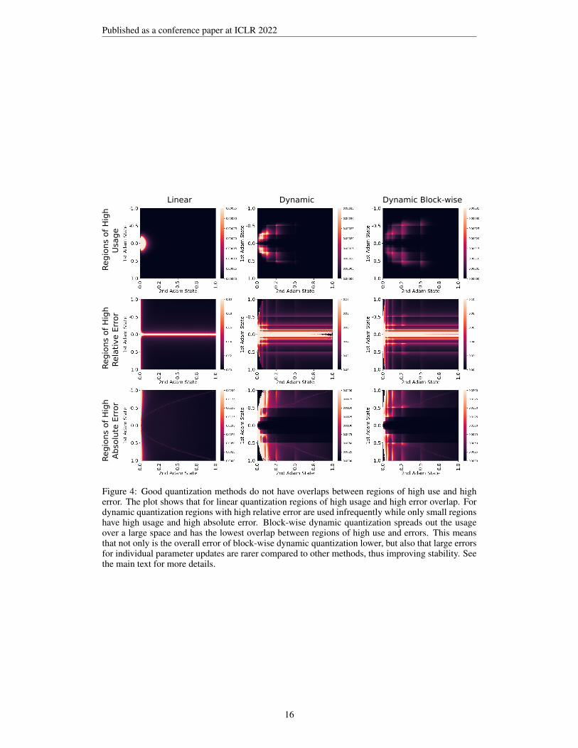
D QUANTIZATION ERROR ANALYSIS

To gain more insights into why block-wise dynamic quantization works so well and how it could beimproved, we performed a quantization error analysis of Adam quantization errors during languagemodel training. Adam quantization errors are the deviations between the quantized 8-bit Adamupdate and the 32-bit Adam updates: |u8 − u16|, where uk = sk1/s

k2 for k bits. See Background

Section 1.1 for details on Adam.

A good 8-bit quantization has the property that, for a given input distribution, the inputs are onlyrarely quantized into intervals with high quantization error and most often quantized into intervalswith low error.

In 8-bit, there are 255×256 possible 8-bit Adam updates, 256 possible values for the first and 256for the second Adam state. We look at the average quantization error of each of these possibleupdates to see where the largest errors are and we plot histograms to see how often do these valueswith high error occur. Taken together, these two perspectives give a detailed view of the magnitudeof deviations and how often large deviations occur.

We study these questions by looking at how often each of the 256 values for both Adam statesare used during language model training. We also analyze the average error for each of the inputsquantized to each of the 256 values. With this analysis it is easy to find regions of high use and higherror, and visualize their overlap. An overlap of these regions is associated with large frequent errorsthat cause unstable training. The quantization error analysis is shown in Figure 4.

The plots show two things: (1) The region of high usage (histogram) shows how often each com-bination of 256×256 bit values is used for the first Adam state s1 (exponentially smoothed runningsum) and the second Adam state s2 (exponentially smoothed running squared sum). (2) The errorplots show for k-bit Adam updates uk = s1/(

√s2 + ε) the mean absolute Adam error |u32 − u8|

and the relative Adam error |u32 − u8|/|u32| averaged over each bit combination. In conjunctionthese plots show which bits have the highest error per use and how often each bit is used. The x-axis/y-axis represents the quantization type range which means the largest positive/negative Adamstates per block/tensor take the values 1.0/-1.0.

We can see that block-wise dynamic quantization has the smallest overlap between regions of highuse and high error. While the absolute Adam quantization error of block-wise dynamic quantizationis 0.0061, which is not much lower than that of dynamic quantization with 0.0067, the plots can alsobe interpreted as block-wise dynamic having rarer large errors that likely contribute to improvedstability during optimization.

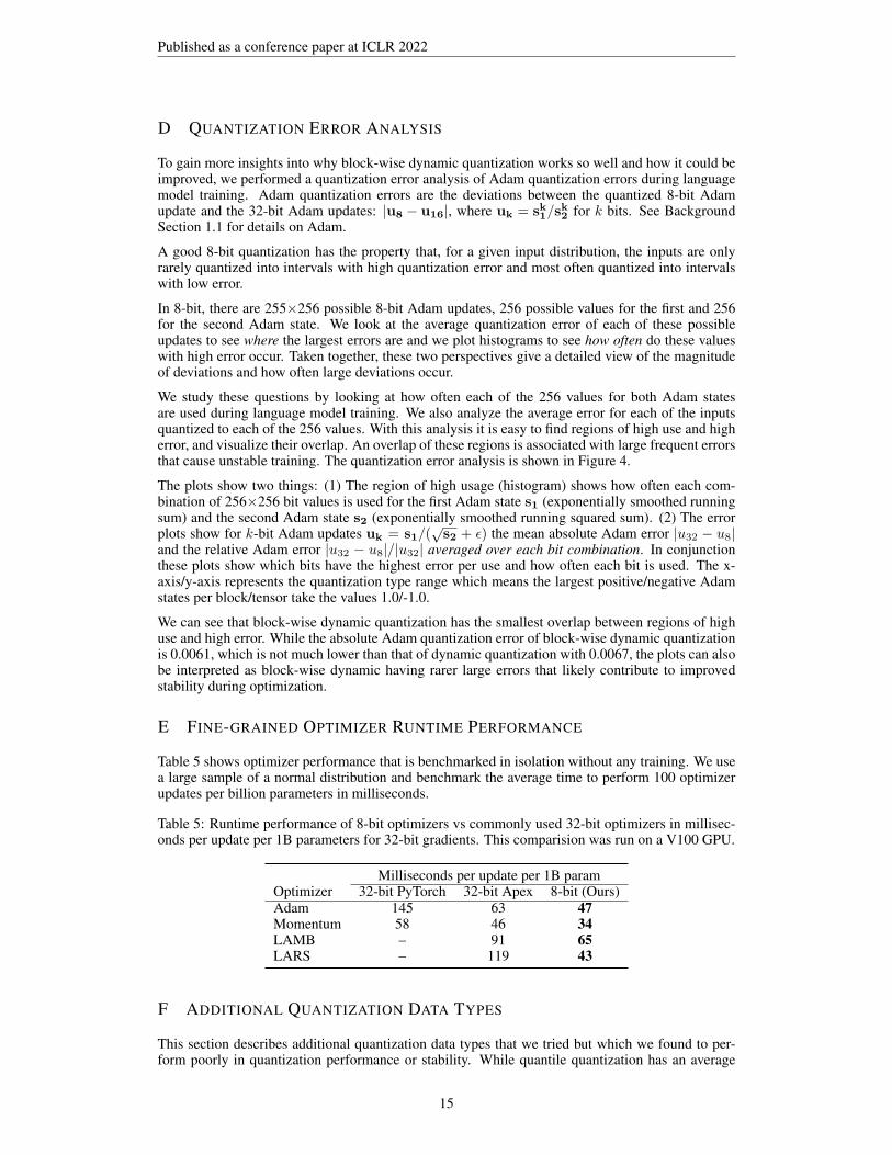
E FINE-GRAINED OPTIMIZER RUNTIME PERFORMANCE

Table 5 shows optimizer performance that is benchmarked in isolation without any training. We usea large sample of a normal distribution and benchmark the average time to perform 100 optimizerupdates per billion parameters in milliseconds.

Table 5: Runtime performance of 8-bit optimizers vs commonly used 32-bit optimizers in millisec-onds per update per 1B parameters for 32-bit gradients. This comparision was run on a V100 GPU.

Milliseconds per update per 1B paramOptimizer 32-bit PyTorch 32-bit Apex 8-bit (Ours)Adam 145 63 47Momentum 58 46 34LAMB – 91 65LARS – 119 43

F ADDITIONAL QUANTIZATION DATA TYPES

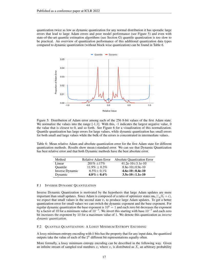
This section describes additional quantization data types that we tried but which we found to per-form poorly in quantization performance or stability. While quantile quantization has an average

15


Dynamic Dynamic Block-wiseLinear

Regio

ns

of

Hig

h U

sage

Regio

ns

of

Hig

h R

ela

tive E

rror

Regio

ns

of

Hig

h A

bso

lute

Err

or

Figure 4: Good quantization methods do not have overlaps between regions of high use and higherror. The plot shows that for linear quantization regions of high usage and high error overlap. Fordynamic quantization regions with high relative error are used infrequently while only small regionshave high usage and high absolute error. Block-wise dynamic quantization spreads out the usageover a large space and has the lowest overlap between regions of high use and errors. This meansthat not only is the overall error of block-wise dynamic quantization lower, but also that large errorsfor individual parameter updates are rarer compared to other methods, thus improving stability. Seethe main text for more details.

16


quantization twice as low as dynamic quantization for any normal distribution it has sporadic largeerrors that lead to large Adam errors and poor model performance (see Figure 5) and even withstate-of-the-art quantile estimation algorithms (see Section G) quantile quantization is too slow tobe practical. An overview of quantization performance of this additional quantization data typescompared to dynamic quantization (without block-wise quantization) can be found in Table 6.

Figure 5: Distribution of Adam error among each of the 256 8-bit values of the first Adam state.We normalize the values into the range [-1,1]. With this, -1 indicates the largest negative value, 0the value that is closest to 0, and so forth. See Figure 6 for a visualization of this normalization.Quantile quantization has large errors for large values, while dynamic quantization has small errorsfor both small and large values while the bulk of the errors is concentrated in intermediate values.

Table 6: Mean relative Adam and absolute quantization error for the first Adam state for differentquantization methods. Results show mean±standard error. We can see that Dynamic Quantizationhas best relative error and that both Dynamic methods have the best absolute error.

Method Relative Adam Error Absolute Quantization ErrorLinear 201% ±17% 41.2e-10±3.1e-10Quantile 11.9% ± 0.3% 8.8e-10±0.9e-10Inverse Dynamic 6.5%± 0.1% 4.6e-10±0.4e-10Dynamic 4.8%± 0.4% 3.5e-10±1.1e-10

F.1 INVERSE DYNAMIC QUANTIZATION

Inverse Dynamic Quantization is motivated by the hypothesis that large Adam updates are moreimportant than small updates. Since Adam is composed of a ratio of optimizer states mt/(

√rt+ ε),

we expect that small values in the second state rt to produce large Adam updates. To get a betterquantization error for small values we can switch the dynamic exponent and the base exponent. Forregular dynamic quantization the base exponent is 100 = 1 and each zero bit decreases the exponentby a factor of 10 for a minimum value of 10−7. We invert this starting with base 10−7 and each zerobit increases the exponent by 10 for a maximum value of 1. We denote this quantization as inversedynamic quantization.

F.2 QUANTILE QUANTIZATION: A LOSSY MINIMUM ENTROPY ENCODING

A lossy minimum entropy encoding with k bits has the property that for any input data, the quantizedoutputs take the value of each of the 2k different bit representations equally often.

More formally, a lossy minimum entropy encoding can be described in the following way. Givenan infinite stream of sampled real numbers xi where xi is distributed as X , an arbitrary probability

17


distribution, a lossy minimum entropy encoding is given by the k-bit quantization map Qmap ∈ R2k

which maps values q ∈ R2k to indices 0, 1, . . . 2k which has the property that if any number ofelements xi from the stream are quantized to xqi we do not gain any information which is predictiveof future xqj>i.

One way to fulfill this property for arbitrary probability distributions X , is to divide the probabilitydistribution function fX into 2k bins where each bin has equal area and the mid-points of these binsare values q of the quantization map Qmap. Empirically, this is equivalent to a histogram with 2k

bins where each bin contains equal number of values.

How do we find the mid-points for each histogram bin? This is equivalent to finding the 2k non-overlapping values x for the cumulative distribution function FX with equal probability mass. Thesevalues can most easily be found by using its inverse function, the quantile function QX = F−1X . Wecan find the mid-points of each of the histogram bins by using the mid-points between 2k+1 equallyspaced quantiles over the range of probabilities [0, 1]:

qi =QX

(i

2k+1

)+QX

(i+12k+1

)2

, (5)

To find q empirically, we can estimate sample quantiles for a tensor T with unknown distribution Xby finding the 2k equally spaced sample quantiles via T’s empirical cumulative distribution function.We refer to this quantization as quantile quantization.

To estimate sample quantiles efficiently, we devise a specialized approximate quantile estimationalgorithm, SRAM-Quantiles, which is more than 75x faster than other approximate quantile esti-mation approaches (Govindaraju et al., 2005; Dunning and Ertl, 2019). SRAM-Quantiles uses adivide-and-conquer strategy to perform sorting solely in fast SRAM. More details on this algorithmcan be found in the Appendix Section G.

F.3 VISUALIZATION: DYNAMIC VS LINEAR QUANTIZATION VS QUANTILE QUANTIZATION

Figure 6 shows the mapping from each to the 255 values of the 8-bit data types to their valuenormalized in the range [-1, 1]. We can see that most bits in dynamic quantization are allocated forlarge and small values. Quantile quantization is introduced in Appendix F.2.

Figure 6: Visualization of the quantization maps for the linear, dynamic and quantile quantization.For quantile quantization we use values from the standard normal distribution and normalize theminto the range [-1, 1].

18


G SRAM-QUANTILES: A FAST QUANTILE ESTIMATION ALGORITHM

To estimate sample quantiles of a tensor one needs to determine the empirical cumulative distributionfunction (eCDF) of that tensor. The easiest way to find the eCDF is to sort a given tensor. Oncesorted, the quantiles can be found by using the value at index i = q × n where i is the index intothe sorted array, q is the desired quantile and n is the total elements in the tensor. While simple,this process of estimating quantiles is computationally expensive and would render training withquantile quantization too slow to be useful.

Similar to other quantile estimation approaches, our GPU algorithm, SRAM-Quantiles, uses a slid-ing windows over the data for fast, approximate quantile estimation with minimal resources. Green-wald and Khanna (2001)’s quantile estimation algorithm uses dynamic bin histograms over slidingwindows to estimate quantiles. Extensions of this algorithm accelerate estimation by using more ef-ficient data structures and estimation algorithms (Dunning and Ertl, 2019) or by using GPUs (Govin-daraju et al., 2005). The main difference between this work an ours is that we only compute a limitset of quantiles that are known a priori – 256, to be exact – while previous work focuses on generalstatistics which help to produce any quantile a posteriori. Thus we can devise a highly specializedalgorithm which offers faster estimation.

The idea behind our algorithm comes from the fact that sorting is slow because it involves repeatedloads and stores from main memory (DRAM) when executing divide-and-conquer sorting algo-rithms. We can significantly improve performance of quantile estimation if we restructure quantileestimation to respect memory hierarchies of the device on which the algorithm is executed.

On a GPU, programmable SRAM – known as shared memory – is 15x faster than DRAM but hasa limit size of around 64 kb per core. The SRAM-Quantiles algorithm is simple. Instead of findingthe full eCDF we find the eCDF for a subset of values of the tensor that fits into SRAM (about 409632-bit values). Once we found the quantiles for each subset, we average the quantiles atomically inDRAM.

This algorithm works, because the arithmetic mean is an unbiased estimator for the population meanand samples quantiles estimated via eCDFs are asymptotically unbiased estimators of the populationquantile (Chen and Kelton, 2001). Thus the more subset quantiles we average, the better the estimateof the tensor-wide quantiles.

For estimating 256 quantiles on a large stream of numbers, our algorithm takes on average 0.064ns to process one element in the stream, whereas the fastest general algorithms take 300 ns (Govin-daraju et al., 2005) and 5 ns (Dunning and Ertl, 2019).

H ADAGRAD COMPARISONS

While the main aim in this work is to investigate how the most commonly used optimizers, such asAdam (Kingma and Ba, 2014) and Momentum (Qian, 1999), can be used as 8-bit variants withoutany further hyperparameter tuning, it can be of interest to consider the behavior of our 8-bit methodsunder different scenarios. For example, one difference between Adam/Momentum and AdaGrad(Duchi et al., 2011) is that AdaGrad accumulates gradients statistics over the entire course of trainingwhile Adam/Momentum use a smoothed exponential decay over time. As such, this could lead tovery different 8-bit quantization behavior where there are large difference between the magnitude ofdifferent optimizer states. Such large differences could induce a large quantization error and degradeperformance of 8-bit optimizers.

To investigate this, we train small 209M parameter language models on the RoBERTa corpus (Liuet al., 2019). We use the AdaGrad hyperparameters introduced by Keskar et al. (2019). Results areshown in Table 7. From the results we can see that our 8-bit methods do not work as well for Ada-Grad. One hypothesis is that this is due to the the wide range of gradient statistics of AdaGrad whichcomes from averaging the gradient over the entire course of training. To prevent poor quantizationin such scenarios, stochastic rounding proved to be very effective from our initial experiments withother 8-bit optimizer. While we abandoned stochastic rounding because we did not see any benefitsfor Adam and Momentum, it could be an effective solution for AdaGrad. We leave such improved8-bit quantization methods for AdaGrad to future work.

19


While AdaGrad falls short in this experiments in terms of perplexity compared to Adam, AdaGrad’sperformance might be improved by adding a momentum term. We leave such improvements forfuture work.

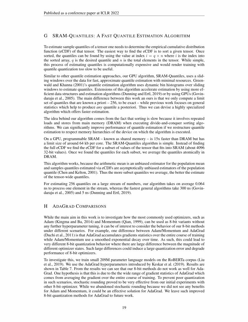
Table 7: AdaGrad compared to Adam performance for a 209M parameter language model on theRoBERTa corpus. The 8-bit methods use stable embedding layer. AdaGrad hyperparamters aretaken from (Keskar et al., 2019).

Optimizer Valid Perplexity

32-bit Adam 16.78-bit Adam 16.4

32-bit AdaGrad 19.48-bit AdaGrad 19.7

I STABLE EMBEDDING LAYER ABLATIONS

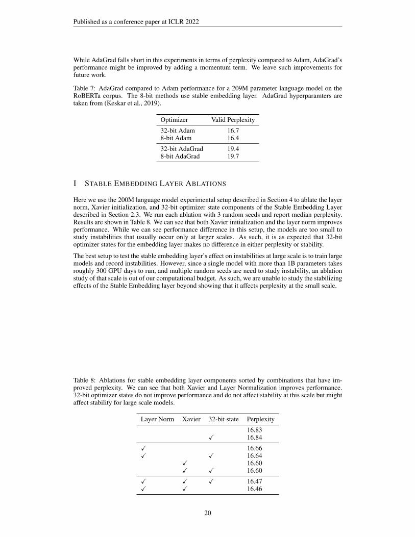
Here we use the 200M language model experimental setup described in Section 4 to ablate the layernorm, Xavier initialization, and 32-bit optimizer state components of the Stable Embedding Layerdescribed in Section 2.3. We run each ablation with 3 random seeds and report median perplexity.Results are shown in Table 8. We can see that both Xavier initialization and the layer norm improvesperformance. While we can see performance difference in this setup, the models are too small tostudy instabilities that usually occur only at larger scales. As such, it is as expected that 32-bitoptimizer states for the embedding layer makes no difference in either perplexity or stability.

The best setup to test the stable embedding layer’s effect on instabilities at large scale is to train largemodels and record instabilities. However, since a single model with more than 1B parameters takesroughly 300 GPU days to run, and multiple random seeds are need to study instability, an ablationstudy of that scale is out of our computational budget. As such, we are unable to study the stabilizingeffects of the Stable Embedding layer beyond showing that it affects perplexity at the small scale.

Table 8: Ablations for stable embedding layer components sorted by combinations that have im-proved perplexity. We can see that both Xavier and Layer Normalization improves performance.32-bit optimizer states do not improve performance and do not affect stability at this scale but mightaffect stability for large scale models.

Layer Norm Xavier 32-bit state Perplexity

16.83X 16.84

X 16.66X X 16.64

X 16.60X X 16.60

X X X 16.47X X 16.46

20

8-bit optimizers via block-wise quantization - arXiv

Documents

Transcript of 8-bit optimizers via block-wise quantization - arXiv