Melbourne, Australia

20 March 2006

Fundamentals of Quantization

Robert M. GrayDept of Electrical Engineering

Stanford, CA 94305

rmgray@stanford.edu http://ee.stanford.edu/˜gray/

The author’s research in the subject matter of these slides was partially supported by the National ScienceFoundation, Norsk Electro-Optikk, and Hewlett Packard.

A pdf of these slides may be found at http://ee.stanford.edu/~gray/shortcourse.pdf

Quantization 1

Introduction

continuous world

discrete representations��

����

@@

@@@R

encoder α

011100100 · · ·

13HH

HHHHj

decoder β

“Picture of a privateer”

������*decoder β

How well can you do it?

What do you mean by “well”?

How do you do it?

Quantization 2

The dictionary (Random House) definition of quantization:

. . . the division of a quantity into a discrete number

of small parts, often assumed to be integral multiples of a

common quantity.

In general, The mapping of a continuous quantity into a

discrete one.

The discrete representation of a signal might be used for

storage in or transmission through a digital link, rendering,

printing, classification, decisions, estimation, prediction, . . .

Discrete points in space might be the location of sensors,

repeaters, resources, Starbucks, mailboxes, fire hydrants, . . .

Quantization 3

Many different kinds of images

Quantization 4

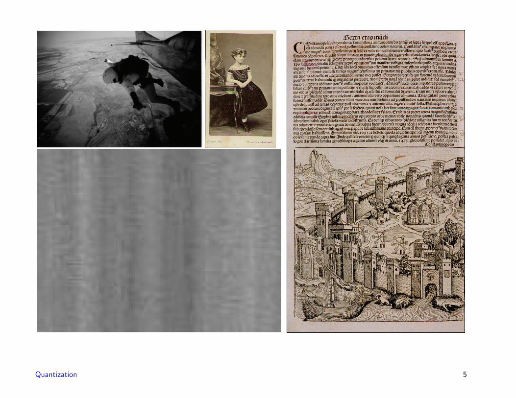
Quantization 5

Images easy to show, but also many other signal types:

• hyperspectral images

• video

• speech

• audio

• sensor data (temperature, precipitation, birdcalls, EKG)

Most are analog of continuous in nature, but need discrete

representation or approximation for digital communication and

storage, classification, recognition, decisions . . .

Quantization 6

Shannon Model of a Communications System

InputSignal

- Encoder - Channel - Decoder -

ReconstructedSignal

Figure 1

Classic Shannon model of point-to-point communication

system

General Goal: Given the signal and the channel, find

an encoder and decoder which give the “best possible”

reconstruction.

Quantization 7

To formulate as precise problem, need

• probabilistic descriptions of signal and channel

(parametric model or sample training data)

• possible structural constraints on form of codes

(scalar, block, sliding block, recursive, predictive)

• quantifiable notion of what “good” or “bad” reconstruction is

(MSE, perceptually weighted distortion, Pe, Bayes risk)

Quantization 8

Mathematical: Quantify what “best” or optimal achievable

performance is.

Practical: How do you build systems that are good, if not

optimal? Theory can provide guidelines for design.

How measure performance?

— SNR, MSE, Pe, bit rates, complexity, cost

Quantization 9

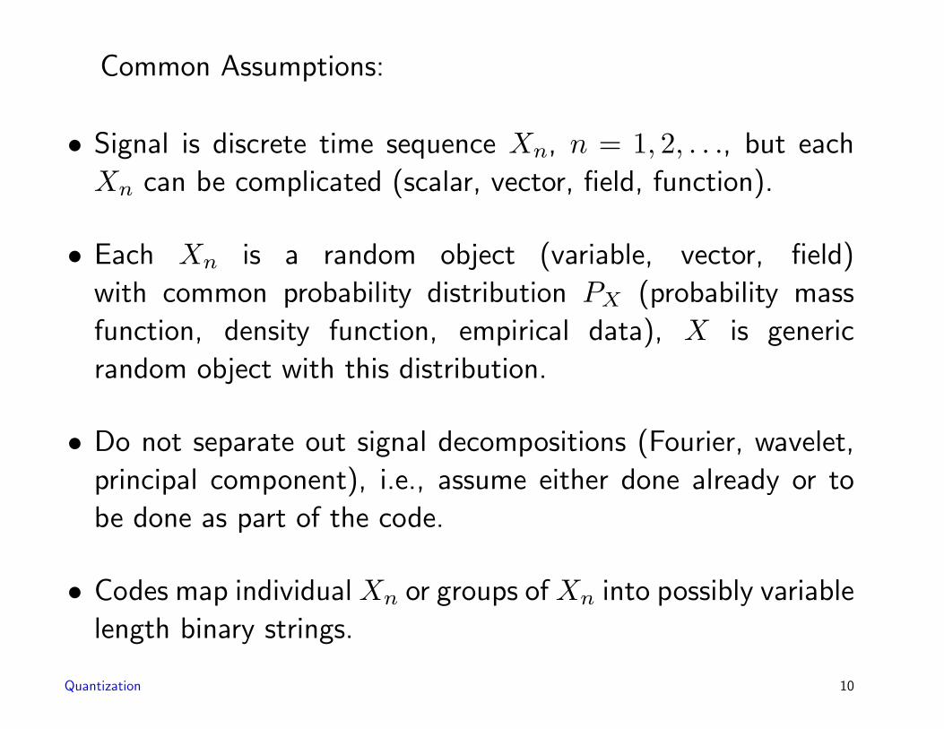
Common Assumptions:

• Signal is discrete time sequence Xn, n = 1, 2, . . ., but each

Xn can be complicated (scalar, vector, field, function).

• Each Xn is a random object (variable, vector, field)

with common probability distribution PX (probability mass

function, density function, empirical data), X is generic

random object with this distribution.

• Do not separate out signal decompositions (Fourier, wavelet,

principal component), i.e., assume either done already or to

be done as part of the code.

• Codes map individualXn or groups ofXn into possibly variable

length binary strings.

Quantization 10

• Binary strings are communicated without further error to

receiver.

These lectures: Survey of fundamentals of quantization:

theories, optimization, algorithms, applications.

Quantization 11

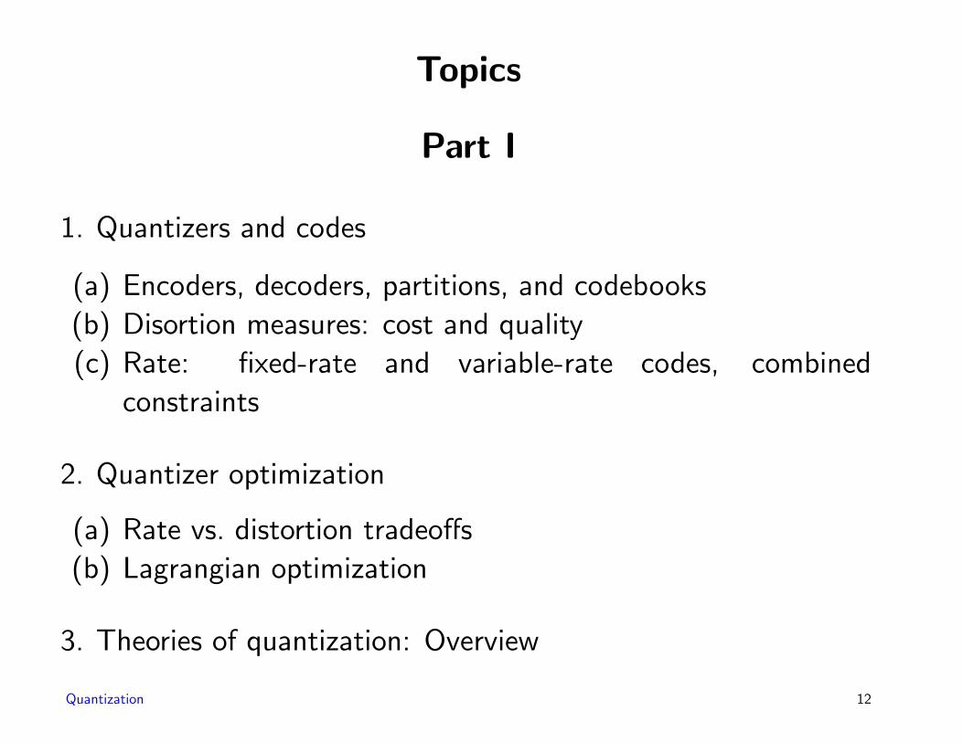
Topics

Part I

1. Quantizers and codes

(a) Encoders, decoders, partitions, and codebooks

(b) Disortion measures: cost and quality

(c) Rate: fixed-rate and variable-rate codes, combined

constraints

2. Quantizer optimization

(a) Rate vs. distortion tradeoffs

(b) Lagrangian optimization

3. Theories of quantization: Overview

Quantization 12

4. Optimality properties and the Lloyd algorithm

(a) Necessary conditions for optimal codes

(b) The Lloyd algorithm: statistical clustering

(c) Variations: Tree-structured quantization, lattice

quantization, transform coding, classified (switched,

composite) quantization, multistage quantization, Gain-

shape quantization

Part II

5. High rate/resolution quantization theory

(a) Uniform scalar quantization

i. Bennett’s classic result, the 6 dB per bit rule

ii. Quantization error and noise, linear “models”

(b) Vector quantization

i. Gersho’s heuristic derivation for vector quantization:

Quantization 13

assumptions and approximations

ii. Quantization point density functions

iii. Fixed-rate, variable-rate, and combined constraints

iv. Survey of rigorous results and a comparison with the

heuristics

v. Asymptotically optimal quantizers

6. Quantizer mismatch, robust codes

7. Gauss mixture modeling

(a) Learning Gauss mixture models as a quantization problem

(b) Quantization, modeling, and statistical classification

(c) Quantization and the Baum-Welch/EM algorithm

8. Closing thoughts

Quantization 14

Part I

Quantization 15

Quantization

Old example: Round off real numbers to nearest integer:

Estimate probability densities by histograms [Sheppard (1898)]

- input

output︸ ︷︷ ︸︸ ︷︷ ︸︸ ︷︷ ︸︸ ︷︷ ︸︸ ︷︷ ︸︸ ︷︷ ︸︸ ︷︷ ︸︸ ︷︷ ︸︸ ︷︷ ︸−4 −3 −2 −1 0 1 2 3 4

In general: a quantizer

• maps each point x in an input space (like the real line, the

plane, Euclidean vector space, function space) into an integer

index i = α(x) (encoder)

• then maps each index into an output β(i) (decoder)

Quantization 16

- input xencoding

decoding

︸ ︷︷ ︸︸ ︷︷ ︸︸ ︷︷ ︸︸ ︷︷ ︸︸ ︷︷ ︸︸ ︷︷ ︸︸ ︷︷ ︸︸ ︷︷ ︸︸ ︷︷ ︸1 2 3 4 5 6 7 8 9 index α(x)↓ ↓ ↓ ↓ ↓ ↓ ↓ ↓ ↓−4 −3 −2 −1 0 1 2 3 4 output β(α(x))

Useful concepts:

• Encoder α⇔ partition of the input space into separate indexed

pieces Si = {x : α(x) = i} partition S = {Si; i ∈ I}.

• Decoder ⇔ reproduction codebook C = {β(i)}

Quantization 17

Everything works if input x is a vector, for example,

• 100 samples of a speech waveform,

• a collection of measurements from a sensor (heat, pressure,

rainfall),

• a 8× 8 block of pixels from a rasterized image

ENCODER

β(1)β(2) β(N)

. . .

x

α(x) = i- -

DECODER

β(1)β(2) β(N)

. . . x = β(i)- -

Encoder is a search Decoder is a table lookup

Computationally intense Simple

Quantization 18

Examples

A scalar quantizer:

- x

codewords

partition cells/atoms

︸ ︷︷ ︸S0

︸ ︷︷ ︸S1

︸ ︷︷ ︸S2

︸︷︷︸S3

︸ ︷︷ ︸S4

β(0)∗

β(1)∗

β(2)∗

β(3)∗

β(4)∗

Two dimensional example

a centroidal Voronoi diagram

(to be explained)

E.g., nearest mailboxes, sensors,

repeaters, stores, facilities

Quantization 19

territories of the male Tilapia

mossambica [G. W. Barlow,

Hexagonal Territories, Animal

Behavior, Volume 22, 1974]

Three dimensions: Voronoi

partition around spheres

http://www-

math.mit.edu/dryfluids/gallery/

Quantization 20

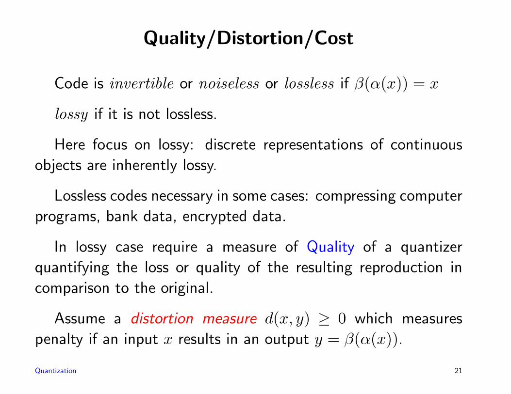
Quality/Distortion/Cost

Code is invertible or noiseless or lossless if β(α(x)) = x

lossy if it is not lossless.

Here focus on lossy: discrete representations of continuous

objects are inherently lossy.

Lossless codes necessary in some cases: compressing computer

programs, bank data, encrypted data.

In lossy case require a measure of Quality of a quantizer

quantifying the loss or quality of the resulting reproduction in

comparison to the original.

Assume a distortion measure d(x, y) ≥ 0 which measures

penalty if an input x results in an output y = β(α(x)).

Quantization 21

Small (large) distortion ⇔ good (bad) quality

To be useful, d should be

• easy to compute

• tractable for analysis

• meaningful for perception or application.

System quality measured by average distortion wrt PX:

D(q) = D(α, β) = E[d(X,β(α(X))] =∫d(X,β(α(X)) dPX(x)

Quantization 22

Examples of distortion measures

• Mean squared error (MSE) d(x, y) = ||x−y||2 =∑k

i=1 |xi−yi|2

• Input or output weighted quadratic, Bx positive definite matrix:

d(x, y) = (x− y)tBx(x− y) or (x− y)tBy(x− y)Used in perceptual coding, statistical classification.

Quantization 23

• X is observation, but unseen Y is desired information

“Sensor” described by PX|Y , e.g., X = Y +W .

Quantize x, reconstruct y = κ(i). Bayes risk C(y, y).

d(x, i) = E[C(Y, κ(i))|X = x]

E[d(X,κ(α(X))] = E[C(Y, κ(α(X)))]

Y -

SENSOR

PX|Y -X -

ENCODER

α - α(X) = i

DECODER

-κ -

β -

Y = κ(i)X = β(i)

Y discrete ⇒ classification, detection

Y continuous ⇒ estimation, regression

Problem: Need to know or estimate PY |X

Quantization 24

Want average distortion small, which can do with bigcodebooks and small cells, but . . .

. . . there is usually a cost r(i) of choosing index i in terms

of storage or transmission capacity or computational capacity —

more cells imply more memory, more time, more bits.

For example,

Quantization 25

• r(i) = ln |C|, All codewords have equal cost. Fixed-rate, classic

quantization.

• r(i) = `(i) — a length function satisfying∑

i e−`(i) ≤ 1

Kraft inequality ⇔ uniquely decodable lossless code exists with

lengths `(i). # of bits required to communicate/store index.

• r(i) = `(i) = − ln Pr(α(X) = i), Shannon codelengths,

E(`(α(X))) = H(α(X)), Shannon entropy. Optimal choice

of ` satisfying Kraft. Optimal lossless compression of α(X).Minimizes required channel capacity for communication.

• r(i) = (1 − η)`(i) + η ln |C|, η ∈ [0, 1] Combined transmission

length and memory constraint.

Average rate R(α) = E[r(α(X))] =∑

i r(i) Pr(α(X) = i)

Quantization 26

Variable vs. fixed rate

• Variable rate codes may require data buffering, expensive and

can overflow and underflow

• Harder to synchronize variable-rate codes. Channel bit errors

can have catastrophic effects.

But variable rate codes can provide superior rate/distortion

tradeoffs.

E.g., in image compression can use more bits for edges, fewer

for flat areas. In voice compression, more bits for plosives, fewer

for vowels.

Quantization 27

Issues

If know distributions,

What is optimal tradeoff of distortion vs. rate?

want both small! theory

How design good codes? (for transmission, storage,

classification, retrieval, segmentation, . . . )

algorithms

If do not know distributions, how use training/learning data

to estimate tradeoffs and design good codes?

statistical or machine learning

Quantization 28

Applications

•

Communications & signal processing:

A/D conversion, data compression.

Compression required for efficient

transmission• send more data in available

bandwidth

• send the same data in less bandwidth

• more users on same bandwidth

and storage• can store more data• can compress for local storage, put

details on cheaper media

Graphic courtesy of Jim Storer.

Quantization 29

• Statistical clustering: grouping bird songs, designing Mao

suites, grouping gene features, taxonomy.

• Placing points in space: mailboxes, recycling centers, wireless

repeaters, wireless sensors

• How best approximate continuous probability distributions by

discrete ones? Quantize space of distributions.

• Estimating local precipitation: g(x) denotes precipitation at

x. Want to estimate total precipitation∫g(x) dx by a sum∑

i∈I g(xi)V (Si), where V (Si) is the area of a region Si.

How best choose the points xi and cells Si? (numerical

integration and optimal quadrature rules)

• Pick best Gauss mixture model from a finite collection.

Quantization 30

• Statistical classification

Microcalcifications in mammograms

Lung nodules in lung CT scans

Quantization 31

Manmade vs. natural200

400

600

800

1000

1200

200

400

600

800

1000

1200

200

400

600

800

1000

1200

Photo vs. not photo

Quantization 32

50

100

150

200

50

100

150

200

50

100

150

200

Text or not text

normal pipeline image field joint longitudinal weld

which is which???

Quantization 33

•Content addressable browsing

Query

Quantization 34

All of these are examples of quantization, but the signals,

distortion measures, and rate definitions can differ widely.

Explore general fundamentals and specific examples ranging

from classic uniform quantization to machine learning.

Quantization 35

Rate vs. distortion

-

6

Average Distortion

.5 1 1.5 2 2.5 3.0Average Rate

vvv

v

f

hhhhhhhhhPPPPPPPPP@@

@@

@@

LL

LL

LL

LL

LL

LL

LLL

vv

vvv

vvvvv

vvv

v

vvv

Every code yields point

in distortion/rate plane:

(R,D).D(α, β) and R(α) measure

costs, want to minimize

both ⇔ Tradeoff

Quantization 36

Optimization problems:

Find Q minimizing D(Q) for constraint R(Q) ≤ R : δ(R)

operational distortion-rate function

Find Q minimizing R(Q) for constraint D(Q) ≤ D : r(D)

operational rate-distortion function

Find Q minimizing unconstrained D(Q) + λR(Q),

Lagrange multiplier λ > 0

Quantization 37

Theories of Quantization

Information Theory Shannon distortion-rate function

D(R)≤ δ(R), achievable in asymptopia of large dimension k

and fixed rate R. [Shannon (1949, 1959), Gallager (1978)]

? Nonasymptotic (Exact) results Necessary conditions for

optimal codes ⇒ iterative design algorithms

⇔ statistical clustering [Steinhaus (1956), Lloyd (1957)]

(Later rediscovered as k-means [MacQueen (1967)])

? High rate theory Optimal performance in asymptopia of fixed

dimension k and large rate R . [Bennett (1948), Lloyd

(1957), Zador (1963), Gersho (1979), Bucklew, Wise (1982)]

Quantization 38

Extreme Points

As λ→ 0, bits are cheap so that R →∞ and D → 0. High

rate theory will describe how rate and distortion trade off in this

case. border between analog and digital

As λ→∞: bits cost far more than distortion

Rate goes to zero, what is best distortion?

Useless in practice, but provides key ideas for general case in

very simple setting.

Only parameter: decoder

Optimal peformance: δ(0) = infy∈AE[d(X, y)]

achieved by codebook with single word argminy∈AE[d(X, y)]

Quantization 39

Example: A = A = <k, squared error distortion, i.e.,

d(x, y) = ||x− y||2 = (x− y)t(x− y)

Then δ(0) = infyE[||X − y||2] achieved by

argminy

E[||X − y||2] = E(X)

Center of mass or centroid.

Example: input-weighted squared error

d(X, X) = (X − X)∗BX(X − X)

centroid is E[BX]−1E[BXX].

Quantization 40

Empirical Distributions

“Training set” or “learning set” L = {xi; i = 0, 1, . . . , L−1}

Empirical distribution is

PL(F ) =#i : xi ∈ F

L=

1L

L−1∑i=0

1F (xi)

Find the vector y that minimizes

E[(X − y)2] =1L

L−1∑n=0

||X − y||2.

Quantization 41

Answer = expectation

y =1L

L−1∑n=0

xi,

the Euclidean center of gravity of the collection of vectors in L.

the sample mean or empirical mean.

Quantization 42

For usual case of fixed λ: Can apply 0 rate result to each

quantizer cell to get optimal decoder.

Since overall goal is to minimize average distortion, optimal

encoder is minimum distortion mapping (“nearest neighbor”):

Given x, choose i to minimize d(x, β(i)) + λr(i).

Add Shannon lossless coding + a pruning rule, get Lloyd

optimality conditions — necessary conditions for a quantizer to

be optimal.

Quantization 43

Lloyd Optimality Properties: Q = (α, β, r, d)

Any component can be optimized for the others.

Encoder α(x) = argmini

(d(x, β(i)) + λr(i)) Minimum distortion

Decoder β(i) = argminy

E(d(X, y)|α(X) = i) Lloyd centroid

Length Function `(i) = − lnPf(α(X) = i) Shannon codelength

Pruning remove any codewords if the pruned code α′, β′, r′ satisfies

D(α′, β′) + λR(α′, r′) ≤ D(α, β) + λR(α, `).E.g., remove i if Pr(α(X) = i) = 0 Pruning

Necessary (but not sufficient) conditions for optimality.

If squared error distortion — decoder is conditional mean

E[X|α(X) = i]: optimal nonlinear estimate of X given α(X)

If empirical distribution — conditional sample average

Quantization 44

For more general input-weighted squared error:

β(i) = E[BX|α(X) = i]−1E[BXX|α(X) = i].

Iteratively optimize each component for the others

⇒ Lloyd clustering algorithm, (k-means, grouped coordinate

descent, alternating optimization, principal points)

Classic case of fixed length, squared error =⇒Voronoi partition (Dirichlet tesselation, Theissen polygons,

Wigner-Seitz zones, medial axis transforms), centroidal

codebook. Centroidal Voronoi partition

Can add constraints, e.g., constrain encoder structure or use

suboptimal search.

Quantization 45

Lloyd Algorithm Examples

Fixed-rate:

Training Sequence & Initial Code Book Centroidal Voronoi

-

6

1-1

1

-1

v1

v2

v4

v3

x

x

x

xx

x

x

x

x

xx

x

S1S4

S2S3

-

6

1-1

1

-1

v1

v2

v4

v3

((((((((((AAAAAAAAAAA

((((((((((

LL

LL

LL

LLL

x

x

x

xx

x

x

x

x

xx

x

S1S4

S2S3

Quantization 46

Variable-rate:

Centroidal Voronoi

diagram for 2D code for

uniform distribution.

x denotes centroid,

o denotes initial

codewords.

Voronoi diagrams common in many fields including biology,

cartography, crystallography, chemistry, physics, astronomy,

meteorology, geography, anthropology, computational geometry.

Quantization 47

Scott Snibbe’s

Boundary Functions

http://www.snibbe.com/scott/bf/

The Voronoi game: Competitive facility

location

http://www.voronoigame.com

Quantization 48

Voronoi DB structure for North American population density.

from http://publib.boulder.ibm.com/infocenter/

Quantization 49

Variations

Problem with general codes satisfying Lloyd conditions is

complexity: minimum distortion encoder requires computation

of distortion between input and output(s) for all codewords.

Exponentially growing computations and memory.

Partial solutions:

Allow suboptimal, but good, components. Decrease in

performance may be compensated by decrease in complexity

or memory. May actually yield a better code in practice.

E.g., by simplifying search and decreasing storage, might be able

to implement an otherwise unimplemental dimension for a fixed

rate R.

Quantization 50

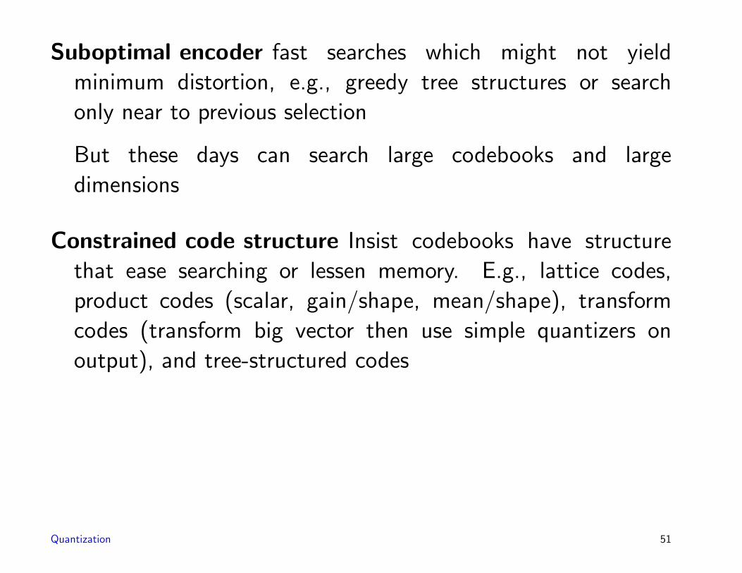
Suboptimal encoder fast searches which might not yield

minimum distortion, e.g., greedy tree structures or search

only near to previous selection

But these days can search large codebooks and large

dimensions

Constrained code structure Insist codebooks have structure

that ease searching or lessen memory. E.g., lattice codes,

product codes (scalar, gain/shape, mean/shape), transform

codes (transform big vector then use simple quantizers on

output), and tree-structured codes

Quantization 51

Tree-structured codes

}-root node �����������

1

label@

@@R

}���

���1}��

����1}������1 } 1111XXXXXX0 } 1110

HHHH

HH0 } 110@

@@

@@@

0 } 10� codeword

terminal node�

���

AAAAAAAAAAA

0

branch�

���

}���

���1}������1} 011

HHHHHH0 }������1 } 0101

XXXXXX0 } 0100@

@@

@@@

0 }�

���

parent

������1}������1 } 0011XXXXXX0 } 0010

HHHH

HH0 }�

��*

child������1 } 0001XXXXXX0 } 0000

siblings

6

?

Quantization 52

Can view each codeword as pathmap through the tree.

Can make code progressive and embedded by producing

reproductions with each bit. Optimally done by centroid of

node, conditional expectation of input given pathmap to that

node.

Suggests suboptimal “greedy” encoder: Instead of finding

best terminal node in tree (full-search), advance through the

tree one node at a time, performing at each node a binary search

involving only two children nodes.

Provides an approximate but fast search of the reproduction

codebook: tree-structured vector quantization (TSVQ)

Quantization 53

BFOS TSVQ design algorithm

Basic idea is taken from methods in statistics for designing

decision trees: (See, e.g., Classification and Regression Treesby Breiman, Friedman, Olshen, & Stone)

• first grow a tree,

• then prune it.

trade off average distortion and average rate.

By first growing and then pruning back can get optimalsubtrees of good trees.

Quantization 54

Growing

Step 0 Begin with optimal 0 rate tree.

Step 1 “Split” node to form rate 1 bit per vector tree.

Step 2 Run Lloyd.

Step 3 If desired rate achieved, stop. Else either

• Split all terminal nodes (balanced tree), or

• Split “worst” terminal node, or

• split in a greedy tradeoff fashion: maximize

λ(t) = | change in distortion if split node t

change in rate if split node t|.

Step 4 Run Lloyd.

Quantization 55

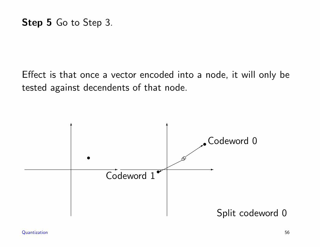
Step 5 Go to Step 3.

Effect is that once a vector encoded into a node, it will only be

tested against decendents of that node.

6

-

v

6

-

ff��

���3

v���

����v

Codeword 0

Codeword 1

Split codeword 0

Quantization 56

6

-

ffAAAK

vAAAUv

v

Only trainingvectors mappedinto codeword 0

are used

�������

HHHHHHj

0 1

�������

HHHHHHj

�

JJ

JJJ

0 1

0 1

Quantization 57

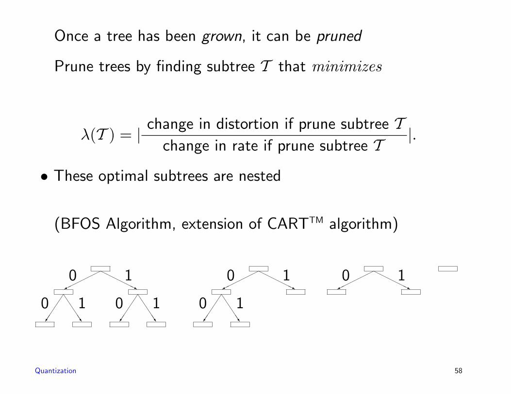
Once a tree has been grown, it can be pruned

Prune trees by finding subtree T that minimizes

λ(T ) = | change in distortion if prune subtree Tchange in rate if prune subtree T

|.

• These optimal subtrees are nested

(BFOS Algorithm, extension of CARTTM algorithm)

�������

HHHHHHj

�

JJ

JJJ

�

JJ

JJJ

0 1

0 1 0 1

�������

HHHHHHj

�

JJ

JJJ

0 1

0 1

�������

HHHHHHj

0 1

Quantization 58

-

6

Average Distortion

.5 1 1.5 2 2.5 3.0Average Rate

vvv

v

f

hhhhhhhhhPPPPPPPPP@@

@@

@@

LL

LL

LL

LL

LL

LL

LLL

vv

vvv

vvvvv

vvv

v

vvv

BFOS finds codes on lower convex hull

Quantization 59

TSVQ Summary: balanced vs. unbalanced, fixed-rate vs.

variable rate

�������

HHHHHHj

�

JJ

JJJ

0 1

0 1

0 1

�

JJ

JJJ

0 1

�

JJ

JJJ

�������

HHHHHHj

�

JJ

JJJ

0 1

0 1 0 1

�

JJ

JJJ

• Sequence of binary decisions. (Each node labeled, do pairwise

minimum distortion.)

• Search is linear in bit rate (not exponential).

• Increased storage, possible performance loss

Quantization 60

• Code is successive approximation (progressive, embedded)

• Table lookup decoder (simple, cheap, software)

• Fixed or variable rate

Quantization 61

Structured VQ

Lattice VQ

Codebook is subset of a regular lattice.

A lattice L in <k is the set of all vectors of the form∑ni=1miui, where the mi are integers and the ui are linearly

independent (usually nondegenerate, i.e., n = k).

E.g., a uniform scalar quantizer (all bin widths equal) is a

lattice quantizer. A product of k uniform quantizers is a lattice

quantizer.

E.g., hexagonal lattice in 2D, E8 in 8D.

Quantization 62

Multidimensional generalization of uniform quantization.

(Rectangular lattice corresponds to scalar uniform quantization.)

Advantages:

• Parameters: scale and support region.

• Fast nearest neighbor algorithms known.

• Good theoretical approximations for performance (special case

of high rate theory)

• Approximately optimal if used with entropy coding: For high

rate uniform quantization approximately minimizes average

distortion subject to an entropy constraint.

Quantization 63

Classified VQ

Switched or composite VQ: Separate quantizer qm =(αm, βm, `m) for each input class (e.g., active, inactive, textured,

background, edge with orientation)

-x VQqm

- i Codeword Index?

Classifier -

m@

@@@R

����! - m Codebook Index

q1 q2 · · · qk

h h h

Decoder: βm(i)

Quantization 64

Transform Coding

X

X1

X2

Xk

-

-

...

-

T

Y

-

-

-

q1

q2

...

qk

Y

-

-

-

T−1

-

-

...

-

X1

X2

Xk

X

Quantization 65

Multistage VQ

X -"!# +

+

−- Q1

X1

6

-E2

Q2-

E2

"!# +

+

+ 6

X1

- X

2-Stage Encoder

X - Q1

- I1X1

-����+−+ 6

X

-

E2Q2

- I2

-

E2

����+−+ 6

E2

-

E3Q3

- I3

-

E3

����+−+ 6

E3

- E4· · ·

Multistage Encoder

Quantization 66

I3

I2

I1

-

-

-

D3

D2

D1

-

E3

E2

X1

?

6"!# + - X

3-stage Decoder

Multistage a special case of TSVQ with a single codebook for

each level.

See also residual VQ where allow smarter searches.

Quantization 67

Shape/Gain VQ (a Product Code)

?

Shape CodebookCs =

{Sj; j = 1, · · · , Ns}Shape/Gain Encoder

X -MaximizeXtSj

- j

?

-Minimize

[g −XtSj)]2- i

Gain CodebookCg =

{gi; i = 1, · · · , Ng}

6

Quantization 68

(i, j) - ROM6

?

Sj

gi

����× - X

Shape/Gain Decoder

Note: Do not normalize input, real-time division a bad idea.

No need, maximum correlation provides minimum MSE.

Two step encoding is optimal! yields best reconstruction.

Overall scheme is suboptimal because of constrained code

structure, but better in practice because allows higher

dimensional VQ for shape.

(Included in LPC and derivative speech coding standards.)

Quantization 69

Part II

Quantization 70

High Rate Theory

High rate quantization theory considers case k fixed and

R→∞

Classic work by Bennett(1948) (also Oliver, Pierce and

Shannon (1948) and Panter and Dite (1951)) (scalar), Zador

(1963), Gersho (1979), Bucklew and Wise (1982) (vectors)

First consider simple uniform scalar quantization. Then

extensions to vector quantization.

In scalar case can do some exact analysis without

approximations, provides insight on common “models” of

quantization error.

Quantization 71

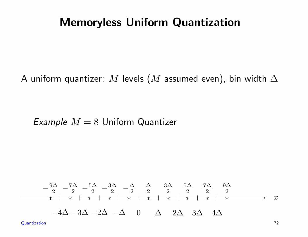
Memoryless Uniform Quantization

A uniform quantizer: M levels (M assumed even), bin width ∆

Example M = 8 Uniform Quantizer

- x∗ ∗ ∗ ∗ ∗ ∗ ∗ ∗ ∗ ∗

−4∆ −3∆ −2∆ −∆ 0 ∆ 2∆ 3∆ 4∆

−9∆2 −7∆

2 −5∆2 −3∆

2 −∆2

∆2

3∆2

5∆2

7∆2

9∆2

Quantization 72

6

- x

q(x)

−4∆−3∆−2∆ ∆ 2∆ 3∆ 4∆

−5∆

−4∆

−3∆

−2∆

−∆

∆

2∆

3∆

4∆

5∆

Quantization 73

q(x) =

quantization levels quantization cells

yM−1 = (M2 −

12)∆; u ∈ RM−1 = [(M

2 − 1)∆,∞)

yk = (−M2 + k + 1

2)∆; u ∈ Rk =

[(−M2 + k)∆, (−M

2 + k + 1)∆)

k = 0, · · · ,M2 − 1

y0 = (−M2 + 1

2)∆; u ∈ R0 = (−∞, (−M2 + 1)∆)

Quantization 74

Quantizer covers no-overload range (no saturation) [−b, b]with M bins of equal width ∆:

b =M

2∆

An input within bin =⇒ midpoint of bin is output. Inputs within

a bin yield an error ≤ ∆2 .

Overload range: Inputs not within a bin cause quantizer overload

(saturation), an error of greater than ∆/2.

Quantization 75

Quantization Noise

Quantizer error ε = q(X)−X so that q(X) = ε+ x.

If input sequence is un, error sequence is

εn = q(Xn)−Xn.

⇒ additive noise “model” of a quantizer:

xn -����+

?

εn

- q(xn)

Quantizer

Quantization 76

Picture is accurate, but further assumptions/approximations

often used in used in communications/signal processing system

analysis and design:

1. εn is independent of the input signal un.

2. εn is uniformly distributed in [−∆/2,∆/2].

3. εn is white, that is, has a flat power spectral density.

If true, uniformly distributed quantization error implies that

the SNR of uniform quantization increases 6 dB for each one bit

increase of rate, (“6 dB per bit rule”)

Quantization 77

Are these reasonable assumptions?

Why Care?If approximations true, approximation permits linearization

of system analysis, can use linear systems techniques to study

overall average distortion, overall quantization noise spectra,

and overall SQNR. Can handle noise and signal terms separately

because linear system, “noise shaping” makes sense. But,

unfortunately

Assumption 1 is ALWAYS false:

The quantization error is a deterministic function of the input.

The two may, however, be uncorrelated:

E[εnXk] = 0 all k, n.

Quantization 78

Approximations (2) and (3) are true exactly if the input signal

is itself memoryless and is uniform over [−b, b]. But (1) not true

even in weak sense: Can show in this case

E(Xnq(Xn)) = −σ2ε . (1)

Quantization 79

More generally, Bennett showed that approximations (2) and

(3) are reasonable if

1. The input is in no-overload region,

2. M asymptotically large,

3. ∆ asymptotically small, and

4. The joint density of input signal is smooth.

Asymptotic (large M , small ∆) or high rate/resolution

quantization theory for uniform quantization. Here give simple

proof of a special case of Bennett’s approximation.

Basic idea: Mean value theorem of Riemann calculus.

Quantization 80

Good News: These assumptions are often reasonable, e.g.,

high rate quantizer of well behaved signal with limited amplitude

range.

Bad News:: Assumptions (2)–(3) are violated in most

systems where the quantizer is inside a feedback loop, e.g., Σ∆modulation, ∆-modulation, and predictive quantization systems.

Assumption (1) is often violated in practice

AND

even if assumptions were reasonable, the Bennett approximations

imply that the signal and quantization error are correlated, not

independent as usually assumed!

Quantization 81

Proof (handwaving) of Bennett’s theorem: First consider

marginal distribution: cdf

Fεn(α) = Pr(εn ≤ α); α ∈ (−∆/2,∆/2)

and pdf

fεn(α) =dFεn(α)dα

.

Then

Pr(εn ≤ α) =M−1∑k=0

Pr(εn ≤ α and Xn ∈ Rk)

Since pdf smooth, mean value theorem of calculus ⇒

Pr(εn ≤ α and Xn ∈ Rk) =∫ −M/2+k∆+α

−M/2+k∆

fXn(β) dβ ≈ fXn(yk)α

Quantization 82

Thus

Pr(εn ≤ α) ≈ α

∆

M−1∑k=0

fXn(yk)∆ ≈ α

∆,

(Riemann sum approximation to integral). Thus

fεn(α) ≈ 1∆

for α ∈ (−∆2,∆2

).

Quantization 83

Multidimensional version same idea:

Pr(εl ≤ αl; l = n, . . . , n+ k − 1) =∑i1,...,ik

Pr(εl ≤ αl and Xl ∈ Ril; l = n, . . . , n+ k − 1),

For αl ∈ (−∆/2,∆/2), l = 1, . . . , k

Pr(εl ≤ αl and Xl ∈ Ril; l = n, . . . , n+ k − 1) =∫ −M/2+k∆+α1

−M/2+k∆

· · ·∫ −M/2+k∆+αk

−M/2+k∆

fXn,...,Xn+k−1(β1, . . . , βk) dβ1 · · · dβk

≈ fXn,...,Xn+k−1(yi1, . . . , yik)α1 · · ·αk

whence

fεn,...,εn+k−1(α1, . . . , αk) ≈

1∆k

.

Quantization 84

Implications:

E[εn] = 0; σ2εn

=∆2

12.

Rε(n, k) = E[εnεk] = σ2εδn−k

fεn|Xl∈Ril; l=n−m,...,n+k(α) =

1∆

for α ∈ (−∆2,∆2

)

Since {q(Xn) = yl} = {Xn ∈ Rl}, ⇒

Rq,ε(n, k) = E[q(Xn)εk]

Quantization 85

=M−1∑l=0

ylE[εk|q(Xn) = yk] Pr(q(Xn) = yk) = 0.

⇒Ru,ε(n, k) = E[Xnεk] = E[(q(Xn)− εn)εk]

= E[q(Xn)εk]−Rε(n, k) = −Rε(n, k),

i.e.,

Ru,ε(n, k) = −σ2εδn−k.

Not uncorrelated! Error uncorrelated with quantizer output, not

with input.

——————-

Quantization 86

In theory, can do second order analysis for any linear system

containing a quantizer using these approximations.

BUT

Problems:

1. Often not known whether or not quantizer can overload (“no-

overload stability” question). Especially true inside feedback

loop.

2. In feedback quantization M is small, typically 2, and ∆ is

not small ⇒ required assumptions for approximations do not

hold!!

Quantization 87

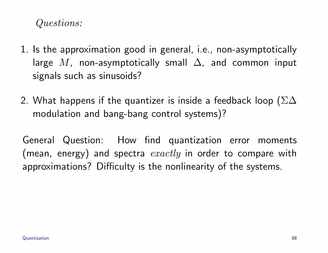
Questions:

1. Is the approximation good in general, i.e., non-asymptotically

large M , non-asymptotically small ∆, and common input

signals such as sinusoids?

2. What happens if the quantizer is inside a feedback loop (Σ∆modulation and bang-bang control systems)?

General Question: How find quantization error moments

(mean, energy) and spectra exactly in order to compare with

approximations? Difficulty is the nonlinearity of the systems.

Quantization 88

Traditional Approaches:

1. The white noise approximation (most common in

communications system design, PCM and Σ∆).

2. Describing function analysis (common in control applications):

Replace nonlinearity by a linearity chosen to minimize MSE

between output of linear and nonlinear systems for a specificinput signal.

3. Use describing function approach, but add white noise to

model error caused by linearization. (Booton applied to Σ∆,

Ardalan and Paulos)

4. Simulation

Quantization 89

5. “Randomize” the quantizer noise by adding a dither signal.

(Roberts, Schuchman, Brinton, Stockham, Lifshitz for PCM)

Fascinating theoretical and practical study, but beware of

published erroneous results (e.g., Jayant and Noll book)

All of the above approaches attempt to linearize the nonlinear

system to permit ordinary linear systems techniques to apply.

The approximations may, however, be bad.

Quantization 90

6. Series expansions of nonlinearity.

6-A. Improve on linearization by adding a few higher order

terms. Hermite polynomials. Can be horrendously

complicated (Arnstein, Slepian for ∆-modulation and

predictive quantization).

6-B. Fourier series of quantizer error. (Example of Rice’s

“Characteristic Function” method (1944) and “transform

method” of Davenport and Root) for memoryless

nonlinearities: Clavier, Panter, Grieg for PCM (1947);

Further contributions by Widrow (1960) and Sripad &

Snyder (1977). Iwersen for ∆ modulation and simplest

Σ∆ modulator. ??

Quantization 91

Characteristic function method has been successful in

analyzing simple systems including uniform quantization of

sinusoids and sums of sinusoids, simple idealized Σ∆ and ∆modulation.

Often shows behavior wildly different from what is predicted

by “theory” using additive noise “model.” E.g., tones in single-

loop Σ∆ modulation or PCM of a sinusoid.

Beware of any analysis based on the assumption of a signal-

independent additive noise model for quantization, it linearizes

a highly nonlinear system. The analysis is simplified, but can

produce garbage results.

Quantization 92

High rate quantization theory: vectors

Traditional form (Zador, Gersho, Bucklew, Wise): pdf f ,

MSE

limR→∞

e2kRδ(R) =

ak||f || kk+2

fixed-rate (R = lnN)

bke2kh(f) variable-rate (R = H), where

h(f) = −∫

dxf(x) ln f(x), ||f ||k/(k+2) =(∫

x

f(x)k

k+2 dx

)k+2k

ak ≥ bk are Zador constants (depend on k and d, not f !)

a1 = b1 =112, a2 =

518√

3, b2 = ?, ak, bk = ? for k ≥ 3

limk→∞

ak = limk→∞

bk = 1/2πe

Quantization 93

Rigorous proofs of traditional cases painfully tedious, but

follow Zador’s original approach:

Step 1 Prove the result for a uniform density on a cube.

Step 2 Prove the result for a pdf that is piecewise constant on

disjoint cubes of equal volume.

Step 3 Prove the result for a general pdf on a cube by

approximating it by a piecewise constant pdf on small cubes.

Step 4 Extend the result for a general pdf on the cube to general

pdfs on <k by limiting arguments.

Quantization 94

Heuristic proofs developed by Gersho: Assume existence of

quantizer point density function Λ(x) for sequence of codebooks

of size N

limN→∞

1N× ( # reproduction vectors in a set S)

=∫

S

Λ(x) dx; all S,

where∫<k Λ(x) dx = 1.

Assume fX(x) smooth,N large, and minimum distortion

quantizer has cells Si locally ≈ scaled, rotated, and translated

copies of convex polytope S∗ achieving

ck = mintesselating convex polytopes S

M(S).

Quantization 95

M(S) =1

kV (S)2/k

∫S

||x− centroid(S)||2

V (S)dx

where define volume V (S) of set S:

V (S) =∫

S

dx

Assumptions + handwaving leads to approximate relationships

among D, H, and N .

Since fX is smooth, the cells are small, and yi ∈ Si,

fX(x) ≈ fX(yi); x ∈ Si

From the mean value theorem of calculus

Quantization 96

PX(Si) =∫

Si

fX(x) dx ≈ V (Si)fX(yi)

hence

fX(yi) ≈PX(Si)V (Si)

.

⇓

D ≈ 1k

N∑i=1

PX(Si)∫

Si

||x− yi||2

V (Si)dx

Quantization 97

For each i, yi is the centroid of Si and hence∫Si

||x− yi||2

V (Si)dx

= minimum MSE for a 0 bit code for a uniformly distributed

random variable on Si = moment of inertia of the region Si

about its centroid

Convenient to use normalized moments of inertia so that

they are invariant to scale.

Define

M(S) =1

kV (S)2/k

∫S

||x− y(S)||2

V (S)dx

where y(S) denotes the centroid of S.

Quantization 98

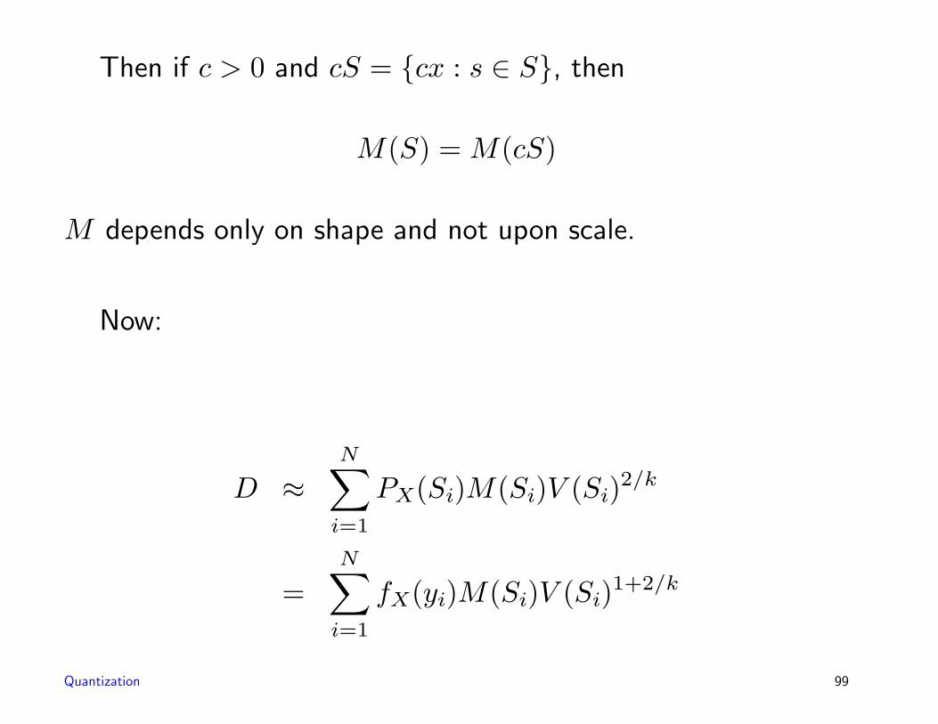
Then if c > 0 and cS = {cx : s ∈ S}, then

M(S) = M(cS)

M depends only on shape and not upon scale.

Now:

D ≈N∑

i=1

PX(Si)M(Si)V (Si)2/k

=N∑

i=1

fX(yi)M(Si)V (Si)1+2/k

Quantization 99

By assumption, there exists a point density function Λ(x):

1N× ( # reproduction vectors in a set S) →

∫S

Λ(x) dx; all S.

∫<k

Λ(x) dx = 1

Then

V (Si) ≈1

λ(yi)

Quantization 100

For large N by Gersho’s assumption M(Si) = ck for all i,

hence

D ≈ ckE[Λ(X)−2/k]N−2/k

This is “Bennett’s integral” or the Bennett approximation.

• Bennett: m = 1/12, k = 1

• Gersho: k ≥ 1

Quantization 101

Entropy of the quantized vector is given by

H = H(α(X)) = −N∑

i=1

PX(Si) logPX(Si),

where PX(Si) =∫

SifX(x) dx.

Again make approximation that

PX(Si) ≈ fX(yi)/(NΛ(yi)) = fX(yi)V (Si)

⇓

H ≈ h(X)− E(log1

NΛ(X)),

where h(X) is the differential entropy.

Quantization 102

Thus for large N

H(α(X)) ≈ h(X)− E(log1

NΛ(X)).

Connection between differential entropy and Shannon entropy

of quantizer output!

Can use to evaluate scalar and vector quantizers, transform

coders, tree-structured quantizers. Can provide bounds.

Used to derive a variety of approximations in compression,

e.g., bit allocation and “optimal” transform codes.

Quantization 103

To summarize:

Df(q) ≈ ckEf

((

1N(q)Λ(X)

)2/k

)Hf(q(X)) ≈ h(X)− E

(log(

1N(q)Λ(X)

))

= lnN(q)−H(f ||Λ),

where

H(f ||Λ) =∫f(x) ln

f(x)Λ(x)

dx

is the relative entropy or Kullback-Leibler number between the

densities f and Λ

Optimizing over Λ using Holder’s inequality or Jensen’s

inequality yields classic fixed-rate and variable-rate results.

Quantization 104

In variable rate case, optimal Λ is uniform, which suggests

lattice codes are very nearly optimal (but need to entropy code

to attain performance).

Note: Gersho’s development ⇒

• For the fixed rate case, cells should have roughly equal partial

distortion.

• For the variable rate case, cells should have roughly equal

volume.

In neither case should you try to make cells have equal

probability (maximum entropy). (Papers extolling “maximum

entropy quantization” have it backwards!)

Quantization 105

Yet oddly enough, Gersho approach implies that optimal fixed

rate quantizers have nearly maximal entropy.

Quantization 106

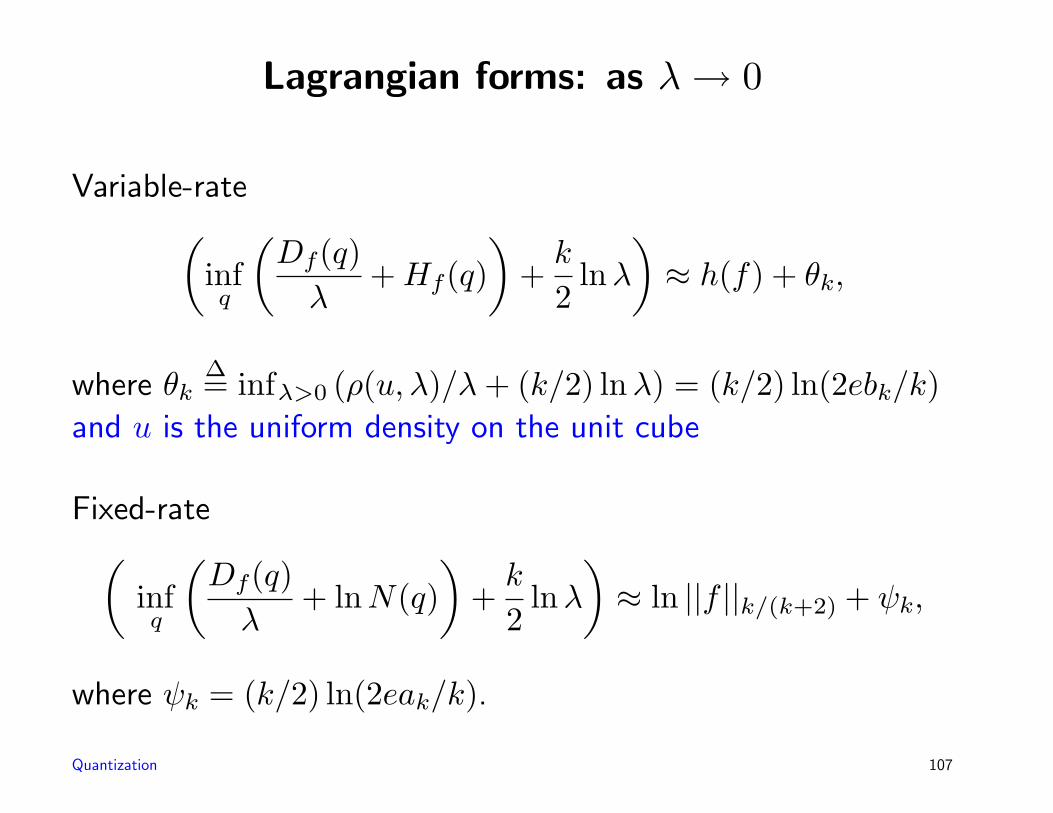
Lagrangian forms: as λ→ 0

Variable-rate(infq

(Df(q)λ

+Hf(q))

+k

2lnλ

)≈ h(f) + θk,

where θk∆= infλ>0 (ρ(u, λ)/λ+ (k/2) lnλ) = (k/2) ln(2ebk/k)

and u is the uniform density on the unit cube

Fixed-rate(infq

(Df(q)λ

+ lnN(q))

+k

2lnλ

)≈ ln ||f ||k/(k+2) + ψk,

where ψk = (k/2) ln(2eak/k).

Quantization 107

Variable-rate: Asymptotically OptimalQuantizers

Theorem ⇒ for λn ↓ 0 there is a λn-asymptotically optimalsequence of quantizers qn = (αn, βn, `n):

limn→∞

(Ef [d(X,βn(αn(X)))]

λn+ Ef`n(αn(X)) +

k

2lnλn

)= θk +h(f)

Worst case: Asymptotic performance depends on f only through

h(f) ⇒ worst case source given constraints is max h source,

e.g., given m and K, worst case is Gaussian.

Quantization 108

Variable-rate codes: Mismatch

What if we design a.o. sequence of quantizers qn for pdf g,

but apply it to f? ⇒ mismatch

Theorem. If qn is λn-a.o. for g, then

limn→∞

Df(qn)λn

+Ef`n(αn(X)) +k

2lnλn = h(f) + θk +H(f ||g).

Quantization 109

if g Gaussian ⇒ limn→∞

(ρ(f, λn, 0, qn)

λn− ρ(g, λn, 0, qn)

λn

)=

−(k/2)+(1/2)Trace(K−1

g Kf + (µf − µg)tK−1g (µf − µg)

)= 0

if µf = µg and Kf = Kg, ⇒ the performance of the code

designed for g asymptotically equals that when the code is

applied to f , a robust code!

Robust and worst-case code ⇒ H(f‖g) measures mismatch

distance from f to Gaussian g with same second-order moments.

Quantization 110

Classified Codes and Mixture Models

Problem with single worst case: too conservative.

Alternative idea, fit a different Gauss source to distinct groups

of inputs instead of the entire collection of inputs. Robust codes

for local behavior.

Given a partition S = {Sm; m = 1, . . . ,M} of <k and a

collection of Gaussian pdfs gm = N (µm,Km), construct an

optimal quantizer qm for each gm.

Two-step (classified) quantizer:

If input vector x ∈ Sm, quantize x using qm.

Encoder sends codeword index along with codebook index m to

decoder.

Quantization 111

Define fm(x) =

{f(x)/pm x ∈ Sm

0 otherwise; pm =

∫Sm

dxf(x)

High rate erformance is

Df(q)λ

+Ef`(α(X)) +k

2lnλ ≈ θk + h(f)+

∑m

pmH(fm||gm)︸ ︷︷ ︸mismatch distortion

What is best (smallest) can make this over all partitions

S = {Sm; m ∈ I} and collections G = {gm, pm; m ∈ I}?⇔ Quantize space of Gauss models using quantizer mismatch

distortion

dQM(x,m) = − ln pm +12

ln (|Km|) +12(x− µm)tK−1

m (x− µm)

Quantization 112

Can use Lloyd algorithm to optimize. Outcome of optimization

is a Gauss mixture.

Alternative to Baum-Welch/EM algorithm.

Lloyd conditions applied to quantizer mismatch distortion:

Encoder (partition) α(x) = argminm dQM(x,m)

Decoder (centroid) gm = argming∈M

H(fm||g) = N (µm,Km).

Length Function L(m) = − ln pm.

Gauss mixture vector quantization (GMVQ)

Quantization 113

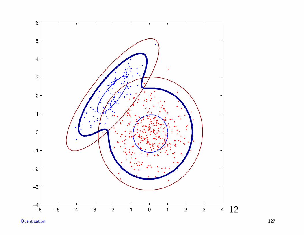
Toy example: Gauss Mixture Design

m1 = (0, 0)t, K1 =[

1 00 1

], p1 = 0.8

m2 = (−2, 2)t, K2 =[

1 11 1.5

], p2 = 0.2

−6 −5 −4 −3 −2 −1 0 1 2 3 4−4

−3

−2

−1

0

1

2

3

4

5

6

−6 −5 −4 −3 −2 −1 0 1 2 3 4−4

−3

−2

−1

0

1

2

3

4

5

6

Quantization 114

Data and Initialization:

−6 −5 −4 −3 −2 −1 0 1 2 3 4−4

−3

−2

−1

0

1

2

3

4

5

6

−6 −5 −4 −3 −2 −1 0 1 2 3 4−4

−3

−2

−1

0

1

2

3

4

5

6

−6 −5 −4 −3 −2 −1 0 1 2 3 4−4

−3

−2

−1

0

1

2

3

4

5

6

Data True pdf superimposed on data Initial code

Quantization 115

−6 −5 −4 −3 −2 −1 0 1 2 3 4−4

−3

−2

−1

0

1

2

3

4

5

6

1Quantization 116

−6 −5 −4 −3 −2 −1 0 1 2 3 4−4

−3

−2

−1

0

1

2

3

4

5

6

2Quantization 117

−6 −5 −4 −3 −2 −1 0 1 2 3 4−4

−3

−2

−1

0

1

2

3

4

5

6

3Quantization 118

−6 −5 −4 −3 −2 −1 0 1 2 3 4−4

−3

−2

−1

0

1

2

3

4

5

6

4Quantization 119

−6 −5 −4 −3 −2 −1 0 1 2 3 4−4

−3

−2

−1

0

1

2

3

4

5

6

5Quantization 120

−6 −5 −4 −3 −2 −1 0 1 2 3 4−4

−3

−2

−1

0

1

2

3

4

5

6

6Quantization 121

−6 −5 −4 −3 −2 −1 0 1 2 3 4−4

−3

−2

−1

0

1

2

3

4

5

6

7Quantization 122

−6 −5 −4 −3 −2 −1 0 1 2 3 4−4

−3

−2

−1

0

1

2

3

4

5

6

8Quantization 123

−6 −5 −4 −3 −2 −1 0 1 2 3 4−4

−3

−2

−1

0

1

2

3

4

5

6

9Quantization 124

−6 −5 −4 −3 −2 −1 0 1 2 3 4−4

−3

−2

−1

0

1

2

3

4

5

6

10Quantization 125

−6 −5 −4 −3 −2 −1 0 1 2 3 4−4

−3

−2

−1

0

1

2

3

4

5

6

11Quantization 126

−6 −5 −4 −3 −2 −1 0 1 2 3 4−4

−3

−2

−1

0

1

2

3

4

5

6

12Quantization 127

−6 −5 −4 −3 −2 −1 0 1 2 3 4−4

−3

−2

−1

0

1

2

3

4

5

6

Converged!Quantization 128

−6 −5 −4 −3 −2 −1 0 1 2 3 4−4

−3

−2

−1

0

1

2

3

4

5

6

−6 −5 −4 −3 −2 −1 0 1 2 3 4−4

−3

−2

−1

0

1

2

3

4

5

6

True source Data driven model

Quantization 129

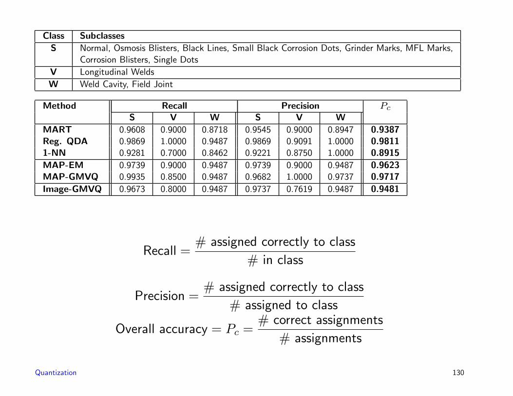
Class Subclasses

S Normal, Osmosis Blisters, Black Lines, Small Black Corrosion Dots, Grinder Marks, MFL Marks,Corrosion Blisters, Single Dots

V Longitudinal Welds

W Weld Cavity, Field Joint

Method Recall Precision Pc

S V W S V W

MART 0.9608 0.9000 0.8718 0.9545 0.9000 0.8947 0.9387Reg. QDA 0.9869 1.0000 0.9487 0.9869 0.9091 1.0000 0.98111-NN 0.9281 0.7000 0.8462 0.9221 0.8750 1.0000 0.8915

MAP-EM 0.9739 0.9000 0.9487 0.9739 0.9000 0.9487 0.9623MAP-GMVQ 0.9935 0.8500 0.9487 0.9682 1.0000 0.9737 0.9717

Image-GMVQ 0.9673 0.8000 0.9487 0.9737 0.7619 0.9487 0.9481

Recall =# assigned correctly to class

# in class

Precision =# assigned correctly to class

# assigned to class

Overall accuracy = Pc =# correct assignments

# assignments

Quantization 130

Parting Thoughts

• Quantization ideas useful for A/D, compression, classification,

detection, and modeling. Alternative to EM for Gauss mixture

design.

• Connections with Gersho’s conjucture on asymptotic optimal

cell shapes (and its implications)

Gersho’s approach provides intuitive, but nonrigorous, proofs

of high rate results based on conjectured geometry of optimal

cell shapes.

Conjecture has many interesting implications that have never

been proved.

Quantization 131

Current research: Find a rigorous development of a variation

on Gersho’s conjecture and use it to prove or disprove several

“folk theorems,” e.g., that ak = bk and optimal fixed rate-

codes have maximal entropy.

• Quantization ideas with weighted quadratic distortion

measures have applications outside of traditional data

compression, especially to statistical classification, clustering,

and machine learning.

Quantization 132