Differences and similarities in work absence behavior

Differences and similaritiesin work absence behavior

Empirical evidence from micro data

Acta Wexionensia No 65/2005 Economics

Differences and similaritiesin work absence behavior

Empirical evidence from micro data

Maria Nilsson

Växjö University Press

Differences and similarities in work absence behavior. Empirical evidence from micro data. Thesis for the degree of Doctor of Philosophy, Växjö University, Sweden 2005

Series editors: Tommy Book and Kerstin Brodén ISSN: 1404-4307 ISBN: 91-7636-462-3 Printed by: Intellecta Docusys, Göteborg 2005

AbstractNilsson, Maria (2005). Differences and similarities in work absence behavior. Empirical evidence from micro data. Acta Wexionensia No. 65/2005. ISSN: 1404-4307, ISBN: 91-7636-462-3. Written in English.

This thesis consists of three self-contained essays about absenteeism. Essay I analyzes if the design of the insurance system affects work absence,

i.e. the classic insurance problem of moral hazard. Several reforms of the sick-ness insurance system were implemented during the period 1991-1996. Using Negative binomial models with fixed effects, the analysis show that both work-ers and employers changed their behavior due to the reforms. We also find that the extent of moral hazard varies depending on work contract structures. The re-forms reducing the compensation levels decreased workers’ absence, both the number of absent days and the number of absence spells. The reform in 1992, in-troducing sick pay paid by the employers, also decreased absence levels, which probably can be explained by changes in personnel policy such as increased use of monitoring and screening of workers.

Essay II examines the background to gender differences in work absence. Women are found, as in many earlier studies, to have higher absence levels than men. Our analysis, using finite mixture models, reveals that there are a group of women, comprised of about 41% of the women in our sample, that have a high average demand of absence. Among men, the high demand group is smaller con-sisting of about 36% of the male sample. The absence behavior differs as much between groups within gender as it does between men and women. The access to panel data covering the period 1971-1991 enables an analysis of the increased gender gap over time. Our analysis shows that the increased gender gap can be attributed to changes in behavior rather than in observable characteristics.

Essay III analyzes the difference in work absence between natives and im-migrants. Immigrants are found to have higher absence than natives when meas-ured as the number of absent days. For the number of absence spells, the pattern for immigrants and natives is about the same. The analysis, using panel data and count data models, show that natives and immigrants have different characteris-tics concerning family situation, work conditions and health. We also find that natives and immigrants respond differently to these characteristics. We find, for example, that the absence of natives and immigrants are differently related to both economic incentives and work environment. Finally, our analysis shows that differences in work conditions and work environment only can explain a minor part of the ethnic differences in absence during the 1980’s.

Keywords: moral hazard, gender difference, immigrants, panel data, count data models, fixed effects, finite mixture models

i

Table of contents Acknowledgements....................................................................................... iii

Introduction....................................................................................................v References ...................................................................................................... ix

Essay I: Work absence and moral hazard – reforms of the Swedish sickness insurance system

1 Introduction ............................................................................................ 1

2 Moral hazard and contract structures...................................................... 4

3 Data and measurement ........................................................................... 8 3.1 Independent variables ....................................................................... 9 3.2 Dependent variables ....................................................................... 13

4 Empirical specification......................................................................... 17

5 Results .................................................................................................. 20 5.1 The baseline model......................................................................... 20

5.1.1 Econometric modeling .......................................................... 20 5.1.2 Estimation results .................................................................. 21

5.2 The extended model........................................................................ 24 5.2.1 Econometric modeling .......................................................... 24 5.2.2 Estimation results .................................................................. 25

6 Conclusions .......................................................................................... 30

References ..................................................................................................... 32

Essay II: Explaining the gender gap in work absence behavior

1 Introduction .......................................................................................... 35

2 Empirical specification......................................................................... 38 2.1 Count data models.......................................................................... 38 2.2 Dealing with heterogeneity ............................................................ 39

2.2.1 Finite mixture models............................................................ 40 2.2.2 Models with fixed and random effects .................................. 41

3 Data ...................................................................................................... 43 3.1 Sampling procedure........................................................................ 43 3.2 Work absence measure................................................................... 43 3.3 Independent variables..................................................................... 45

4 Results .................................................................................................. 49 4.1 Gender differences in absence levels.............................................. 49

4.1.1 Model selection..................................................................... 49 4.1.2 Empirical results ................................................................... 50

4.2 Analyzing the increased gender gap............................................... 54 4.2.1 Model selection ..................................................................... 54

ii

4.2.2 Estimation results .................................................................. 54

5 Conclusions .......................................................................................... 58

References ..................................................................................................... 60 Appendix ....................................................................................................... 63

Essay III: Immigrants in the Swedish sickness insurance system –

ethnic differences in work absence behavior

1 Introduction .......................................................................................... 65

2 The Swedish sickness insurance system............................................... 67

3 Modeling work absence behavior ......................................................... 69

4 Data and empirical specification .......................................................... 74 4.1 Sampling procedure........................................................................ 74 4.2 Work absence measures ................................................................. 75 4.3 Empirical specification................................................................... 77 4.4 Independent variables..................................................................... 80

5 Empirical results................................................................................... 82 5.1 Ethnic differences in factors explaining absence behavior ............. 82

5.1.1 Model selection ..................................................................... 82 5.1.2 Estimation results .................................................................. 84

5.2 Ethnic differences in predicted number of absent days................... 87

6 Concluding remarks.............................................................................. 88

References ..................................................................................................... 90 Appendix A.................................................................................................... 95 Appendix B.................................................................................................... 96 Appendix C.................................................................................................... 97 Appendix D.................................................................................................... 98

iii

AcknowledgementsAfter being a part of my life for such a long time, this thesis has finally come to an end. Fortunately, my subject of academic interest, absenteeism, has become more and more relevant over the years. But not only has time improved my the-sis; the support of the people around me has helped as well. First, I’d like to thank my two advisors, so different from each other, yet both so valuable. Mårten Palme, my advisor for the last three years, has contributed to the progress of my work through his vast knowledge of work absence research and his econometric skills. Thank you so much for your confidence in me. Your friendly encouragement during my periods of doubt has been invaluable. Your enormous optimism and your countless suggestions have always brought the work a step further. Inga Person, my first advisor, introduced me to absenteeism by putting me in touch with Malmöhus läns landsting. The project developed into my licen-tiate thesis through Inga’s tremendous support. I will always be indebted to you, Inga, for your support of my efforts to combine writing with the other parts of life.

Lennart Flood was the discussant for my licentiate thesis and also for the final seminar for this thesis. Your suggestions and challenging questions strongly con-tributed to my work – thank you!

During the work with my licentiate thesis, David Edgerton and Curt Wells offered valuable econometric advice. Agneta Kruse contributed her enthusiasm for research on social securities and careful reading of manuscripts. Thanks for all of your help.

Jonas Månsson was the one who convinced me to attend the PhD program. Thank you for always taking the time to help, whatever the problem. Lennart De-lander has read several versions of my manuscript and I am grateful for all the excellent comments. We are so lucky that you still want to work for CAFO when you could spend your time fishing. There are many other colleagues who have read this and commented on it throughout the years and even more who have contributed to the warm atmosphere at Växjö University – thanks to you all!

Mimi Möller helped me correct the English language. Thanks for your excellent suggestions; now are all the remaining errors my own responsibility.

Financial support from Växjö University, Lund University, Malmöhus läns landsting, KEFU and HSF is gratefully acknowledged.

Växjö, April 2005

Maria Nilsson

v

Introduction

In Sweden, work absence due to personal illness is covered by a separate public sickness insurance system. This system was introduced in 1955 and has been re-formed several times since then. Its intention is to support individuals by replac-ing lost labor earnings when work capacity is temporarily prevented due to ill-ness. The sickness insurance system is one of the greatest welfare programs in Sweden. In 2002, the total cost for public sickness benefits was about 2% of GDP (Palmer, 2003).

Throughout the years, the utilization of the sickness insurance system has fluctu-ated remarkably. The fluctuations are greater than what can be entitled to varia-tion in health status. Earlier research has shown that the utilization of the sick-ness insurance system varies with the utilization of other income security pro-grams and with labor market conditions in general. Several studies have shown that work absence is related to unemployment rates and compensation levels within the insurance system (Johansson & Palme, 1996, 2002; Johansson & Brännäs, 1998; Henrekson & Persson, 2004). Research on work absence behav-ior is of special importance since the absence levels have increased dramatically in the last decade. Sweden is today one of the countries possessing the highest absence rates (Nyman et. al., 2002). The high levels of absence have major im-plications for the absent individuals, their employers, and society. Not only would it be financially positive if the absence rates decreased, but as number of people of working age shrinks, all contributions of worked hours are of impor-tance to society. As such, there is a broader motivation do conduct research con-cerning work absence behavior than just the strict medical justification.

This thesis consists of three self-contained essays about absenteeism. Although I have chosen not to integrate them into one framework, they never-the-less share some common features. Work absence is defined in all three as time away from work that is not anticipated or scheduled and where the reason is said to be per-sonal illness. The eligibility for compensation only requires the individuals’ own perception of their health such as it prohibits them from performing their regular work. After a week of absence, a doctor’s certificate is needed for extension of the benefit period. Illness can be seen as a continuum and the ability to attend work gradually decreases with health deficiencies. As such, the choice of whether or not to go to work is not only a medical decision but also an individual decision based on how trying it is to attend work. Just how trying it is depends on both the ability and motivation to attend (Steers & Rhodes, 1984). Ability is based on perceived health such as it makes working possible. Health is incorpo-rated in the analysis through the inclusion of health indicators and through con-sidering that health status is one of the main sources of unobserved heterogene-ity. Turning to the factor of motivation to attend work, we find separate explana-tions. In Essay I, absence is analyzed within a moral hazard perspective and the importance of economic incentives for attending work is scrutinized. Motivation

vi

level is also influenced by the essential components of the occupation held. Both work pleasure and position in the hierarchy can be expected to affect motivation to attend work. The relation between characteristics of the work contract held and work absence is another important focus of the first essay.

The analyses in Essays II and III depart from labor supply theory and focus on other aspects of motivation. In analyzing gender and ethnic differences in ab-sence behavior, the role of family responsibility is examined by the inclusion of information on family situation. Work environment affects motivation as well. Poor working environments increase the risk of health problems, thus decreases ability to attend work while also decreasing the motivation to attend. A risk- averse person would try to minimize exposure to unhealthy environments. To consider the influence of work environment several indicators are included in the analyses.

The empirical orientation provides another common feature; the three essays are all based on panel micro data. The data used in Essay I is especially collected for the study and consists of personnel records from a large public employer. The data cover the period 1991-1996, a period for which it is impossible to procure official register data on absence. From 1992 onwards, employers became respon-sible for sickness benefits for short-term absences, therefore there are no official figures covering these absences. The other two essays are based on data from the Swedish Level of Living Surveys combined with register data from the National Social Insurance Board and cover the period 1971-1991. The entire period is used in Essay II to study gender differences in work absence, while Essay III, which analyzes ethnic differences in absence, is based on data from the later part of the period.

A special feature of Essay I is the access to several different measures of absence that cover short as well as long-term absences and duration as well as incidence. Even though the other two essays do not have the same rich information on dif-ferent absence measures, the dependent variables in the three essays are all non-negative integer values. I thus base all my analyses on count data models as us-ing models based on continuous distributions would be inappropriate (Cameron & Trivedi, 1986).

Moral hazard and the sickness insurance system

The sickness insurance system forms part of the work contract between worker and employer. In Essay I, analyses are made to reveal if the design of the insur-ance system affects work absence, i.e., the classic insurance problem of moral hazard. The reforms of the sickness insurance system during the period studied (1991-96) are expected to affect the incentives for reducing absence for both workers and employers. Reforms affecting compensation rules serve as exoge-nous variation in the cost of absence and are thus possible to use for analyzing the extent of moral hazard by the workers. In addition, I analyze if the extent of moral hazard differs due to other work contract characteristics. As the data are

vii

personnel records I have information of the work contract structure for each in-dividual and can analyze if workers with different kinds of contracts act differ-ently in the face of the reforms. The reform of 1992 that made employers respon-sible for sick pay can be expected to affect employer behavior, as their cost of absence increased. Thus, that reform can be analyzed from a moral hazard per-spective as well.

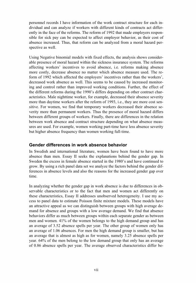
Using Negative binomial models with fixed effects, the analysis shows consider-able presence of moral hazard within the sickness insurance system. The reforms affecting workers’ incentives to avoid absence, i.e. reforms making absence more costly, decrease absence no matter which absence measure used. The re-form of 1992 which affected the employers’ incentives rather than the workers’, decreased work absence as well. This seems to be caused by increased monitor-ing and control rather than improved working conditions. Further, the effect of the different reforms during the 1990’s differs depending on other contract char-acteristics. Male nighttime worker, for example, decreased their absence severity more than daytime workers after the reform of 1993, i.e., they are more cost sen-sitive. For women, we find that temporary workers decreased their absence se-verity more than permanent workers. Thus the presence of moral hazard differs between different groups of workers. Finally, there are differences in the relation between work absence and contract structure depending on what absence meas-ures are used. For example, women working part-time have less absence severity but higher absence frequency than women working full-time.

Gender differences in work absence behavior

In Swedish and international literature, women have been found to have more absence than men. Essay II seeks the explanations behind the gender gap. In Sweden the excess in female absence started in the 1980’s and have continued to grow. By using a rich panel data set we analyze the factors behind the gender dif-ferences in absence levels and also the reasons for the increased gender gap over time.

In analyzing whether the gender gap in work absence is due to differences in ob-servable characteristics or to the fact that men and women act differently on these characteristics, Essay II addresses unobserved heterogeneity. I use my ac-cess to panel data to estimate Poisson finite mixture models. These models have an attractive appeal as we can distinguish between groups with high average de-mand for absence and groups with a low average demand. We find that absence behaviors differ as much between groups within each separate gender as between men and women. 41% of the women belongs to the high demand group and has an average of 3.52 absence spells per year. The other group of women only has an average of 1.06 absences. For men the high demand group is smaller, but has an average that is almost as high as for women, namely 3.25 absence spells per year. 64% of the men belong to the low demand group that only has an average of 0.86 absence spells per year. The average observed characteristics differ be-

viii

tween the low and high absence demand groups, but so do the response to differ-ent characteristics.

Using Negative binomial model with fixed effects we find that absence patterns have changed during the period studied. For example, during the 1980’s small children did not have such a positive relation to male absence as it had during the 1970’s. Women with small children on the other hand, had even less absence during the later part of the period. The increased gender gap over time can be at-tributed to changed behavior rather than changed observable characteristics. One possible explanation to changed behavior is that new groups of women have en-tered the labor market; groups with observed and unobserved characteristics re-sembling the ones of the high absence demand group in our sample.

Ethnic differences in work absence

Today, ten percent of the Swedish population is comprised of first-generation immigrants. Earlier studies show great integration problems regarding the prob-ability of acquiring a job, income development and inclusion in the social secu-rity systems (Hansen & Löfström, 2000; Hammarstedt, 2001). It is also known that immigrants have higher absence levels compared to natives, though rela-tively few studies have been made (Kindlund, 1995; Akhavan & Bildt, 2004; Gustavsson & Österberg, 2004). The cause of these higher levels, according to most explanations, is that many immigrants are found in occupations with poor work environment. Immigrants have problems getting a job and when they fi-nally acquire one, they are absent from work more than natives. These high ab-sence rates make the process of integration even more difficult.

My analysis shows interesting ethnical differences in work absence. In applying Negative binomial models with fixed effects, I find that diverse factors affect work absence for natives and immigrants and that natives and immigrants act on these factors differently. I find that economic incentives play a larger role in ex-plaining work absence behavior for immigrant women than for native women. For men, I find that a poor working environment affects immigrants and natives in opposite directions. For women, I find support for the hypothesis that speciali-zation within the household affects work absence behavior.

Decomposition of the ethnic differences in work absence reinforces earlier find-ings that differences in work environment are one important explanation. But our main result is that there are intrinsic ethnic differences in work absence that can-not be explained by differences in the observed characteristics. Although the rich data enables inclusion of, for work absence studies, unusually many observed characteristics; we can only explain a small part of the discrepancy in work ab-sence. Thus there are rather differences in unobserved heterogeneity that can ex-plain ethnic differences in work absence.

ix

ReferencesAkhavan, S & Bildt, C (2004). Arbetsvillkor, hälsa och sjukfrånvaro bland invandrade

kvinnor, Arbetslivsrapport, 2004:21, Arbetslivsinstitutet.

Cameron , A C & Trivedi, P K (1986). “Econometric Models Based on Count Data: Comparisons and Applications of Some Estimators and Tests”. Journal of Applied

Econometrics, vol 1, issue 1, p 29-53.

Gustavsson, B & Österberg, T (2004). “Ursprung och förtidspension” i Ekberg, J (red) Egenförsörjning eller bidragsförsörjning. Invandrare, arbetsmarknad och välfärdssta-

ten, antologi utgiven av integrationspolitiska maktutredningen, SOU 2004:21.

Hammarstedt, M (2001). Making a living in a new country. Doctoral thesis, Växjö Uni-versity Press, Växjö.

Hansen, J & Löfström, M (2000). “Immigrant assimilation and welfare participation: Do immigrants assimilate into or out-of welfare?”. Journal of Human Resources, vol 38:1, p 74-98.

Henrekson, J & Persson, M (2004). “The Effects on Sick Leave of Changes in the Sick-ness Insurance System”. Journal of Labor Economics, vol 22, no 1, p 87-114.

Johansson, P & Brännäs, K (1998). “A household model for work absence”. Applied Eco-

nomics, vol 30, p 1493-1503.

Johansson, P & Palme, M (1996). “Do economic incentives affect work absence? Empiri-cal evidence using Swedish micro data”. Journal of Public Economics, vol 59, p 195-218.

Johansson, P & Palme, M (2002). “Assessing the effect of public policy on worker absen-teeism”. The Journal of Human Resources, vol 37:2, p 281-409.

Kindlund, H (1995). “Förtidspensionering och sjukfrånvaro 1990 bland invandrare och svenskar” in Invandrares hälsa och sociala förhållanden. SoS-rapport 1995:5, Social-styrelsen, Stockholm.

Nyman, K, Bergendorff, S & Palmer, E (2002). Den svenska sjukan: sjukfrånvaron i åtta

länder, Rapport till Expertgruppen för studier i offentlig ekonomi, ESO, Finansdepar-tementet, Regeringskansliet, Stockholm.

Palmer, E (2003). “Svensk sjukskrivning i ett internationellt perspektiv” in Swedenborg, B (red) Varför är svenskarna så sjuka?, SNS Förlag, Stockholm.

Steers, R & Rhodes, S (1978). “Major Influences on Employee Attendance: A Process Model”. Journal of Applied Psychology, vol 63, no 4, p 391-407.

Essay I

Essay I

Work absence and moral hazard – reforms of the Swedish sickness insurance system

1 Introduction In Sweden, as in many other countries, work absence due to illness is covered by a public sickness insurance system. The intention is to support individuals when work capacity is temporary lost due to illness by replacing forgone labor earn-ings. The absence levels have though steadily increased for almost a decade and in year 2002, the total cost for public sickness benefits reached almost 2% of GDP (Palmer, 2003). During the first three years of the new century, the number of days covered by benefits from either sickness insurance or early retirement scheme, recounted as number of full-year workers, corresponded to about 14 per-cent of the population, aged 20-64 years (Högstedt et. al., 2004). As is true for all insurances, the sickness insurance system is characterized by problems of asym-metric information. The problems of adverse selection are solved in Sweden by making the system compulsory and thus include both high and low risk groups. It is possible to report personal sickness for seven days on the basis of personal assessment. Eligibility for compensation only requires the individuals’ percep-tions of their personal health to render them unfit for regular work. First on the eighth day of absence is a doctor’s certificate required. As such, it is reasonable to expect presence of moral hazard within the Swedish sickness insurance sys-tem, i.e. that the compensation level affects the utilization of the insurance.

During the first part of the 1990’s, several reforms were implemented in the Swedish sickness insurance system. First, reforms that changed the individual’s incentive for not being absent by changing the share of lost earnings not covered by the insurance. Second, reforms that gave the individual employer incentives to reduce work absence by moving the financial responsibility for replacing for-gone earnings to the employer. As both workers’ and employers’ incentives to avoid absence are changed due to the reforms, we can expect moral hazard from both sides. The reforms of the early 1990’s have rarely been thoroughly ana-lyzed; the reform of 1992, when the financial responsibility was moved to the employer, has not been analyzed at all. One of the main reasons to the few

1

2

evaluations of the reforms is the lack of data. From 1992, the first two weeks in each absence spell are no longer included in official data on work absence.1

The data used in this study include absence information for more than 23,000 workers employed at a large Swedish public health care organization at the be-ginning of 1991. These workers are followed each year until the end of 1996. Each time a worker is absent from work, the employer registers it. Our access to these personnel records, in contrast to official data, gives us the possibility of analyzing both long-term and short-term work absence during the first half of the 1990’s. Personnel records also minimize measurement errors common in self-reported absence data.

The data allows for analyzing several aspects of work absence behavior. First, we analyze if the design of the public sickness insurance system affects work ab-sence, i.e. the classical insurance problem of moral hazard. The reforms that changed the compensation rules within the sickness insurance system serve as exogenous variation in the workers’ cost of absence. We can thus analyze whether the workers exhibit moral hazard. Due to the reform in 1992, the em-ployers’ cost of absence increased and they received increased incentives to im-prove working conditions as well as to increase their monitoring and control of the workers’ absence behavior. Thus, this reform serves as exogenous change in the employer’s incentives to avoid absence and we can analyze whether the em-ployers exhibit moral hazard as well.

Reforms of the sickness insurance system can be viewed as changes in the work contract – the agreement between the employer and the worker on what is to be done and at what compensation. The occupation, the number of working hours, the work schedule, the work conditions as well as the wage, fringe benefits, and social security benefits are all parts of the work contract. Our data includes in-formation of work contract characteristics as if a person works part or full time, if the contract is permanent or temporary and what kind of occupation a person has. Secondly, we analyze if the reforms of the sickness insurance system have different effects on absence depending on these other contract characteristics. We thus analyze if different groups of workers respond differently to the re-forms, i.e. if the extent of moral hazard differ depending on the work contract structure.

The present study broadens several aspects of the previous literature on work ab-sence and public policy. The impact of some of the reforms has been analyzed before but then using aggregate data. In contrast to Henrekson & Persson (2004), our use of micro data allow us to analyze the effects of the reforms on individual

––––––––– 1 Since then the length of employers responsibility has changed several times, but during the period

studied the number of days was 14.

2

3

absence behavior.2 The importance of work contract structures has also been ana-lyzed earlier using aggregate data. Arai & Skogman Thourise (2005) found a negative correlation between sick rates and the share of temporary workers. Our data allows for an extended analysis of differences in absence behavior between permanent and temporary workers as we can analyze whether workers with per-manent and temporary contracts act differently on the reforms, i.e. if they exhibit differences in moral hazard.

An additional extension of earlier studies is that the data allows us to consider different aspects of absence through the use of several different absence meas-ures. We define work absence as time spent away from work that is not antici-pated or scheduled and where the cause is said to be personal illness.3 Based on earlier findings, we then use a categorization into four different measures of ab-sence: total number of absent days (absence severity), total number of absence spells (absence frequency), frequency of 1-day absences (attitudinal absence) and finally frequency of absences of 3 days or longer (medical absence). The four measures are all on an annual basis and are not distinct separate measures with strict dividing lines between them. They are rather non-exclusive measures that together cover different absence characteristics. We expect presence of moral hazard to affect the different absence measures in different ways. Spell measures are found to be better measures of voluntary absence or related to discretionary reasons for absence while day measures emphasize long-term absence or absence more likely caused by serious illness (Gellatly, 1995; Scott & McLelland, 1990).

All of our absence measures can only take nonnegative integer values which lead us to count data models. Our use of panel data, in contrast to cross-sectional data used in many earlier studies, enables estimation methods that can handle the un-observed heterogeneity likely to be found in absence data. Such unobserved het-erogeneity would imply correlation over time between the absences of a specific individual and neglecting the correlation would bias our estimates. Unobserved heterogeneity may also cause problems with endogeneity. It is reasonable to ex-pect several of the unobserved individual specific effects to be correlated, not only with absence, but with our independent variables as well. To be able to con-sider such dependence we estimate Negative binomial models with fixed as well as random effects. The reforms of the sickness insurance system are though strictly exogenous why we are able to analyze their causal effect on absence.

The analysis shows clear evidence of moral hazard within the Swedish sickness insurance system. The reforms of 1993 and 1996, reducing the compensation

––––––––– 2 Henrekson & Persson (2004) used grouped data and tried to correct the underreported official ab-

sence figures by adding the average number of days absent in spells shorter than 14 days found in a survey of private establishments.

3 In Sweden, social security is divided into two parts when it comes to illness; one part covers lost earnings due to personal illness and the other part covers lost earnings due to absence for taking care of sick children. This also means that in the employer’s register of absence the two different grounds for absence are kept separate.

3

4

levels, decreased absence, no matter which absence measure used. Our findings are thus a reinforcement of the study by Henrekson & Persson (2004). A more austere sickness insurance system decreases work absence. The reform in 1992, which affected the employers’ incentives rather than the workers’, decreased work absence as well, i.e. the employers exhibit moral hazard as well. It seems as it was rather due to increased monitoring and control than due to improved work conditions. Further, the effect of the different reforms during the 1990’s differs depending on other contract characteristics. Male nighttime workers, for example, decreased their absence severity more than daytime workers after the reform in 1993. For women, we find that temporary workers decreased their ab-sence severity more than permanent workers. Thus the presence of moral hazard differs between different groups of workers. Finally, there are differences in the relation between work absence and contract structure depending on what absence measure used. For example, women working part-time have less absence sever-ity but higher absence frequency compared to women working full-time.

The paper is organized as follows: In Section 2 there is a theoretical discussion of expected relations between moral hazard and contract structures. Section 3 presents the data and variables used. The econometric specification is discussed in Section 4 while the estimation results are presented in Section 5. Finally, con-clusions are discussed in Section 6.

2 Moral hazard and contract structures

Illness is a continuum and in many cases the individual can use his or her discre-tion whether to go to work or not. In Sweden it is possible to report in sick for seven days on the basis of a personal health assessment. From the eighth day of absence a doctor’s certificate is required.4 Thus the choice of whether or not to attend work is not only a medical decision but also an individual decision based on how trying it would be to attend work.

The primary cost of absence is forgone earnings not covered by sickness bene-fits.5 The impact of a sickness benefit system is unambiguous as the existence of a sickness benefit system lowers the cost of absence, i.e. the benefits lower the economic incentives to avoid absence. Table 1 shows the contents of the reforms of the Swedish sickness insurance system during the period studied. The begin-ning of the 1990’s was characterized by cutbacks in most of the Swedish social security systems as a response to public deficits. Sickness benefits were signifi-cantly changed several times. As can be seen in Table 1, the replacement rate in 1991 was cut to 65% for the first three days of sick leave, and to 80% between

––––––––– 4 In rare cases, after repeated absence, the employer can ask for a doctor’s certificate earlier. But this

can only be done after an agreement with the union representative. 5 Normally, lost earnings are only replaced up to an income ceiling. In the organization studied, how-

ever, those with an income above the ceiling receive additional replacement.

4

days 4 and 90. In 1992 the responsibility for the first fourteen days of sick leave was, as already mentioned, moved from the public authorities to the employers. In 1993 one qualification day (with 0% benefits) was introduced and later in the same year the replacement rate for spells longer than one year was cut to 70%. In 1996 the replacement rate was fixed at 75% regardless of the duration of the ab-sence spell.

Table 1. The sickness benefit system in Sweden. Replacement rates in percentage of the daily wage (RFV,1995, 1997). Day December 1, 1987 March 1, 1991 January 1, 1992 in – – – sick leave February 30, 1991 December 31, 1991 March 31, 1993 Sickness benefit Sickness benefit Sick pay Sickness benefit 1 90 + 10a 65 + 10 75 65 + 10 2–3 90 + 10 65 + 10 75 65 + 10 4–14 90 + 10 80 + 10 90 80 + 10 15–90 90 + 10 80 + 10 80 + 10 91–365 90 + 5 90 90 366– 90 + 5 90 90

Day April 1, 1993 July 1, 1993 January 1, 1996 in – – – sick leave June 30, 1993 December 31, 1995 December 31, 1996 Sick pay Sickness Sick pay Sickness Sick pay Sickness benefit benefit benefit 1 0 0 0 0 0 0 2–3 75 65 + 10 75 65 + 10 75 75 4–14 90 80 + 10 90 80 + 10 75 75 15–90 80 + 10 80 + 10 75 + 10 91–365 80 80 75 + 10 366– 80 70(80)b 75 a) + 10% from collective agreements, for salaried employees. b) 80% in some cases if the person is in a rehabilitation program

The reforms of the sickness benefit system in 1991, 1993 and 1996 all increased the individual’s cost of absence, thus we can expect a decline in absence. We ex-pect, above all, absences of short duration, i.e. those that the individual decides upon personally, to decrease when the cost of absence increases. In particular, we expect attitudinal absence (1-day absences) to decline after 1993 since the re-placement for such absences is non-existent from then on. Earlier studies have found a strong relationship between absence and the cost of absence (Barmby, Orme & Treble, 1991, 1995; Drago & Wooden, 1992; Johansson & Palme, 1996, 2002; Johansson & Brännäs, 1998; Henrekson & Persson, 2004).

There are other costs of absence than those of forgone earnings. Sickleave may be penalized in the form of decreased probability of receiving promotions or merit wage increases and/or an increased likelihood of being dismissed. The pos-sible existence of a penalty for absence, in the form of risk of being dismissed, may act as a disciplinary effect in line with the efficiency wage theory (Shapiro & Stiglitz, 1984). It is reasonable to expect the disciplinary effect to be greater for temporary workers than for permanent workers. High absence rates decrease

5

6

the probability of receiving an extended contract, thus we expect temporary workers to have less absence.6 We can expect increased ”absence” screening of presumptive workers after the reform of 1992 since the employer’s cost for ab-sence then increased. It might then follow that people on temporary contracts find it harder to procure permanent contracts which could affect their absence behavior. A negative relation between temporary work contracts and absence has been found in several earlier studies (Edgerton, Kruse & Wells, 1996; Arai & Skogman Thoursie, 2005).

Penalties for work absence are likely to be more severe if unemployment is high, since the cost of losing a job is higher as it is more difficult to find new employ-ment. This means that we would expect work absence to decrease with rising un-employment. This is in line with explanations based on discipline effects (Arai & Skogman Thoursie, 2005; Henrekson & Persson, 2004; Lantto, 1991). There are also so-called composition theories (Leigh, 1985; Bäckman, 1998; Vogel, Kind-lund & Diderichsen, 1992), which state that in hard times, it is the individuals with poor health that have problems getting and keeping a job. This speaks for fewer absences of long durations when unemployment is high. But it is not un-reasonable to assume that there could also be effects in the opposite direction. High unemployment can in itself cause poor health, both for the unemployed and for the employed that are worried about losing their jobs (Bäckman, 1992; Östlin et al., 1996). So, theoretically we cannot say whether unemployment increases or decreases absence, but most empirical findings show a negative relation (for ex-ample Henrekson, Lantto & Persson, 1992; Henrekson & Persson, 2004).

The employer can further try to reduce absence by controlling workers by using different kinds of monitoring devices.7 The reform introducing sick pay in 1992 could therefore be expected to result in increased monitoring. The employer’s cost of absence differs depending on the nature of the job. In occupations where workers are easily replaced or where tasks can be accumulated, the employer’s costs may be lower. Such occupations might therefore not be as intensely moni-tored and the penalties for absence might be fewer. On the other hand, if a person is not replaced and tasks are accumulated during absence, the cost of absence is higher for the absent person. So even if these occupations are less monitored, they may still induce less absence as absence are more costly for the individual worker. There might also be other occupational differences in the cost of absence in the form of loss of on-the-job training or possibilities of advancement.

The organization in focus for this study is strictly hierarchic and a worker’s posi-tion in this hierarchy probably affects his/her work attitudes. If persons consider themselves an integral part of the production process, they probably have higher

––––––––– 6 Repeated temporary contract are very common in the Swedish public health care system. It does not

only have to be the case of a contract being prolonged or not; it might also be whether or not it is possible to receive good references for future employments.

7 This can be difficult since illness to a great extent is private information.

6

7

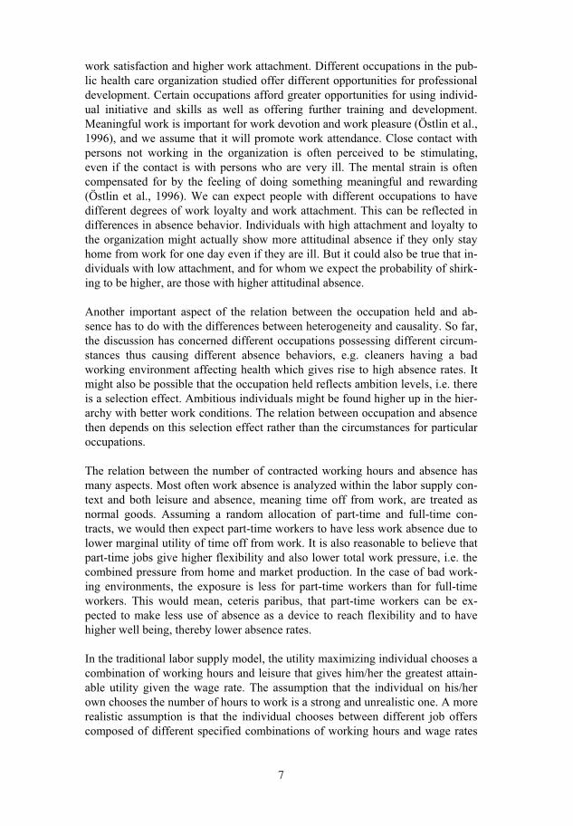
work satisfaction and higher work attachment. Different occupations in the pub-lic health care organization studied offer different opportunities for professional development. Certain occupations afford greater opportunities for using individ-ual initiative and skills as well as offering further training and development. Meaningful work is important for work devotion and work pleasure (Östlin et al., 1996), and we assume that it will promote work attendance. Close contact with persons not working in the organization is often perceived to be stimulating, even if the contact is with persons who are very ill. The mental strain is often compensated for by the feeling of doing something meaningful and rewarding (Östlin et al., 1996). We can expect people with different occupations to have different degrees of work loyalty and work attachment. This can be reflected in differences in absence behavior. Individuals with high attachment and loyalty to the organization might actually show more attitudinal absence if they only stay home from work for one day even if they are ill. But it could also be true that in-dividuals with low attachment, and for whom we expect the probability of shirk-ing to be higher, are those with higher attitudinal absence.

Another important aspect of the relation between the occupation held and ab-sence has to do with the differences between heterogeneity and causality. So far, the discussion has concerned different occupations possessing different circum-stances thus causing different absence behaviors, e.g. cleaners having a bad working environment affecting health which gives rise to high absence rates. It might also be possible that the occupation held reflects ambition levels, i.e. there is a selection effect. Ambitious individuals might be found higher up in the hier-archy with better work conditions. The relation between occupation and absence then depends on this selection effect rather than the circumstances for particular occupations.

The relation between the number of contracted working hours and absence has many aspects. Most often work absence is analyzed within the labor supply con-text and both leisure and absence, meaning time off from work, are treated as normal goods. Assuming a random allocation of part-time and full-time con-tracts, we would then expect part-time workers to have less work absence due to lower marginal utility of time off from work. It is also reasonable to believe that part-time jobs give higher flexibility and also lower total work pressure, i.e. the combined pressure from home and market production. In the case of bad work-ing environments, the exposure is less for part-time workers than for full-time workers. This would mean, ceteris paribus, that part-time workers can be ex-pected to make less use of absence as a device to reach flexibility and to have higher well being, thereby lower absence rates.

In the traditional labor supply model, the utility maximizing individual chooses a combination of working hours and leisure that gives him/her the greatest attain-able utility given the wage rate. The assumption that the individual on his/her own chooses the number of hours to work is a strong and unrealistic one. A more realistic assumption is that the individual chooses between different job offers composed of different specified combinations of working hours and wage rates

7

8

(Dickens & Lundberg 1993). Contract structures, concerning the number of con-tracted working hours, are a result of the employers’ response to the nature of their production technology and the characteristics of the labor force. If the workers are only offered certain kinds of contracts, they are forced into certain time allocation combinations that may not guarantee that their chosen contractual hours equal their desired working hours. If the contractual working hours are more than the desired, workers may use absence in order to reach their optimal time allocation (Dunn & Youngblood, 1986). If the contractual number of work-ing hours on the other hand is less than desired, it is reasonable to assume that the marginal utility of absence is less than otherwise.

If there are young children in the family many women choose part-time con-tracts. If a person without children chooses to work part-time, it could be due to some other reason to the high valuing of time off from work. In Sweden, with high replacement rates in case of absence, it is though hard to see why a person would choose a part-time contract because of bad health–it would be much better to get a full-time contract and receive sickness benefits when ill. It is more rea-sonable to believe that employers only offer part-time contracts to individuals with bad health. No matter how the process leading to a part-time contract works, we see that selection effects can be of importance when evaluating the re-lation between work contracts and absence. Selection effects may actually lead to higher absence among part-time workers. In earlier studies, part-time work has though most often been found to decrease absence (Edgerton, Kruse & Wells, 1996; Chaudhury & Ng, 1992; Drago & Wooden, 1992).

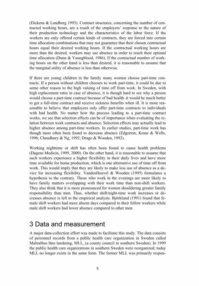
Working nighttime or shift has often been found to cause health problems (Dagens Medicin, 1999, 2000). On the other hand, it is reasonable to assume that such workers experience a higher flexibility in their daily lives and have more time available for home production, which is one alternative use of time off from work. This would imply that they are likely to make less use of absence as a de-vice for increasing flexibility. VandenHeuvel & Wooden (1995) formulates a hypothesis to the contrary. Those who work in the evenings are more likely to have family matters overlapping with their work time than non-shift workers. They also think that it is more pronounced for women shouldering greater family responsibility than men. Thus, whether shift/night-time work increases or de-creases absence is left to the empirical analysis. Björklund (1991) found that fe-male shift workers had more absent days compared to their fellow workers while male shift workers had lower absence compared to other men.

3 Data and measurement

A major data-collection effort was made to facilitate this study. The data consists of personnel records from a public health care organization in Sweden called Malmöhus läns landsting, MLL, (a county council in southern Sweden). In 1999 the public health care organizations in southern Sweden were reorganized; today MLL no longer exists in the same form. The former MLL was primarily respon-

8

9

sible for health care (including dental care), in a broad sense. Since it was such a large organization, however, administration and other service departments were also quite extensive. MLL also engaged in health care education as well, both at the high school and university/college levels.

In January 1991, MLL employed 23,654 persons, of whom approximately 80% were women. The personnel records from 1991 to 1996 were used to construct the variables presented below. Some of the employees had miscoded variables and/or missing values which is why the panel data consists of 19,139 observa-tions for the first year of the study. The number of employees at MLL declined rapidly during the first half of the 1990’s due to budget cuts within the public sector in Sweden.8 The panel is, therefore, unbalanced and many persons em-ployed in January 1991 quit before the end of December 1996; we are left with 10,941 individuals still employed in December 1996.9

3.1 Independent variables

Since one of the main focuses of this study is whether moral hazard is related to different aspects of the work contract, several variables describing the work con-tract have been constructed (see Table 2). For every year of the study we have individual information on the contracts held on 30 June. We have to make the as-sumption that the same contract characteristics hold for the entire year. The vari-able temp reflects whether the contract is temporary or permanent, part reflects whether a person works part-time or full-time and night reflects whether it is night time or day time work. To cover the work situation aspect of the contract, the variable occ is included. There are a vast number of occupations within the organization studied. To make data tractable, we had to combine and reduce them into six occupational variables. We have aggregated occupations that re-quire about the same amount of education and/or where the work situations could be considered to be about the same. Unfortunately we have no information regarding wages, but the way the variable occ is constructed makes it a proxy not only for the work situation but also for wages.

The reforms in the sickness benefit system are included as dummy variables. We decided, after thorough consideration, only to include the reforms of 1992, 1993 (the first of the two) and 1996 (ref92, ref93 and ref96). The other reforms during the period studied are minor and probably not well acknowledged by the work-ers. Unfortunately the reform of 1991 which increased the cost of absence cannot

––––––––– 8 In 1992 there was also a major reform, which shifted the responsibility for the care of the elderly

from the regional to the municipality level. This accounts for some of the huge drop in number of employees for the period studied.

9 Attrition will not be a problem as long as the reason for leaving MLL is uncorrelated with any un-observed variables affecting absence. This is probably a reasonable assumption since when the public sector makes cuts in numbers of employees it is done according to tenure.The only reason why tenure would be correlated in any way to absence would be if work attachment or loyalty were correlated with tenure. We here assume that this is not the case.

9

10

be analyzed since we do not have any data before 1991.10 Earlier studies have shown that the reform of 1991 reduced absence (Henrekson & Persson, 2004; Johansson & Palme, 2002).

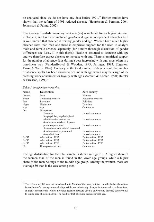
The average Swedish unemployment rate (ue) is included for each year. As seen in Table 2, we have also included gender and age as independent variables as it is well known that absence differs by gender and age. Women have much higher absence rates than men and there is empirical support for the need to analyze male and female absence separately (for a more thorough discussion of gender differences see Essay II in this thesis). Health is assumed to decrease with age and we therefore expect absence to increase with age. There is empirical support for the number of absence days during a year increasing with age, most often in a non-linear way (VandenHeuvel & Wooden, 1995; Paringer, 1983; Edgerton, Kruse & Wells, 1996). Contrary to the total number of days absent, the number of absence spells has been shown to decline with age which may be a sign of in-creasing work attachment or loyalty with age (Mathieu & Kohler, 1990; Hetzler & Ericsson, 1991).11

Table 2. Independent variables.

Name Description Zero dummy Gender Man Woman Temp Temporary contract Permanent contract Part Part-time Full-time Night Night-time Day-time Age Age Continuous Occ Occupation 2 – nurse 1– assistant nurse 3 – physician, psychologist & administrative executives 1– assistant nurse 4 – cleaners, washers & transportation personnel 1– assistant nurse 5 – teachers, educational personnel & administrative personnel 1– assistant nurse 6 – technicians 1– assistant nurse Ref92 After reform 1992 Before reform 1992 Ref93 After reform 1993 Before reform 1993 Ref96 After reform 1996 Before reform 1996 Ue Unemployment rate Continuous

The age distribution for the total sample is shown in Figure 1. A higher share of the women than of the men is found in the lower age groups, while a higher share of the men belongs to the middle age group. Among the women, more are over age 50 than is the case among men.

––––––––– 10 The reform in 1991 was not introduced until March of that year, but, two months before the reform

is too short of a time span to make it possible to evaluate any changes in absence due to the reform. 11 In many international studies the exact absence measure used is unclear and absence could be due

to taking care of sick children. The need for that of course decreases with age.

10

11

Figure 1. Age distribution.

0

5

10

15

20

25

30

35

40

-19 20-29 30-39 40-49 50-59 60-

Age

%

Women

Men

Figure 2 shows the distribution over different occupations for men and women. As we can see the distribution is quite different for men and women.

Figure 2. The distribution over different occupations—see Table 2 for description of the

different occupation categories.

0

5

10

15

20

25

30

35

40

45

1 2 3 4 5 6

Occupation

%

Women

Men

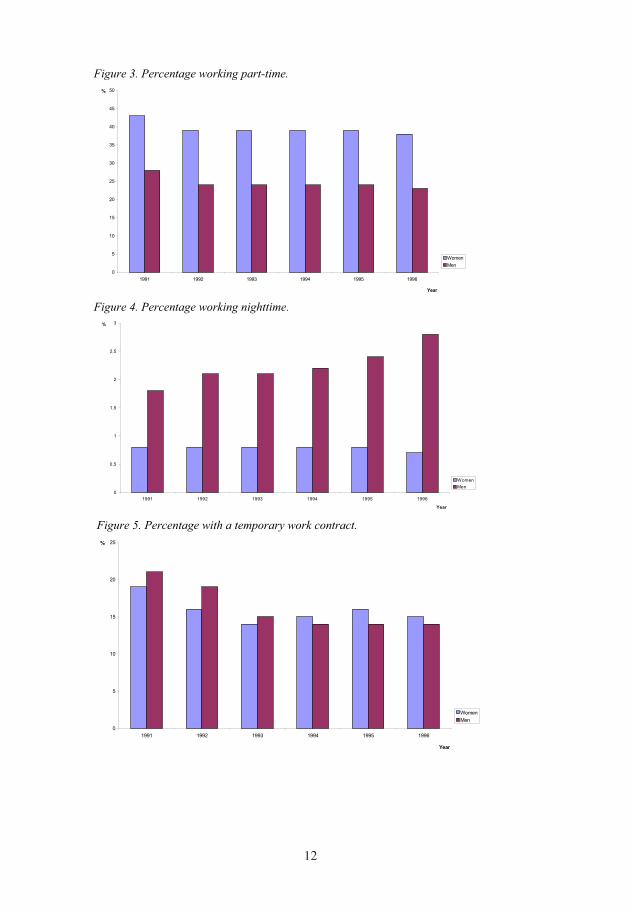
Men and women not only have different occupations within the health care or-ganization but other aspects of the work contract differ as well. Women work part-time to a greater extent than men do (Figure 3), while men more often work nighttime (Figure 4). In the beginning of the 1990’s, men were more often on a temporary contract but this changed during the period studied so that at the end of the period, temporary contracts were more common among the women. (Fig-ure 5).

11

12

Figure 3. Percentage working part-time.

0

5

10

15

20

25

30

35

40

45

50

1991 1992 1993 1994 1995 1996

Year

%

Women

Men

Figure 4. Percentage working nighttime.

0

0,5

1

1,5

2

2,5

3

1991 1992 1993 1994 1995 1996

Year

%

Women

Men

Figure 5. Percentage with a temporary work contract.

0

5

10

15

20

25

1991 1992 1993 1994 1995 1996

Year

%

Women

Men

12

13

3.2 Dependent variables

From the employer’s register we obtain information on every individual absence spell for each worker for all years studied. From this data we construct measures that cover our four dimensions of absence. The measures used are all on an an-nual basis:

Absence severity: total number of days absent ( number of days scope)12

Absence frequency: total number of absence spells with a scope of 100%

Attitudinal absence: frequency of 1-day absences (of scope 100%)

Medical absence: 1) frequency of absences of 3-7 days (scope 100%)

2) frequency of absences of 8 days or longer (scope 100%)13

The reason for splitting the medical absence into two separate measures is due to the Swedish sickness benefit rules. It is not until the 8th day in a sick leave that the worker needs a certificate from a doctor. Thus we could expect different ef-fects on medical absence depending on which of the two measures, short or long medical absence, that we analyze.

As Table 3 shows, in the total sample, women have higher levels for all absence measures except short medical absence.

Table 3. Descriptive statistics. Means with standard deviations in parentheses.

Women Men

Absence measure

Absence severity 17.17 (47.60) 15.00 (44.83)

Absence frequency 1.43 (2.15) 1.37 (2.14)

Attitudinal absence 0.42 (0.96) 0.39 (0.98)

Short medical absence 0.39 (0.83) 0.39 (0.84)

Long medical absence 0.30 (0.71) 0.27 (0.67)

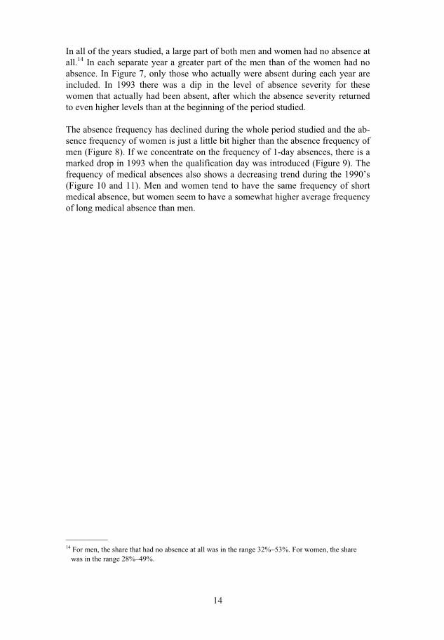
Figure 6 to 11 presents the development of absence for the years studied. Figure 8 shows a decreasing trend in absence severity for men while the trend for women decreases until 1993 and then flattens out. Women have higher absence severity than men for all years studied, although in 1993 the average number of absent days was nearly the same for men as for women.

––––––––– 12 We know how many days every spell lasted and also its scope (in Sweden one can be on sick leave

part-time e.g. 25%, 50% or some other percentage). 13 This should actually be all absences with spells of 8 days or longer whatever their scope. One

weakness of the data, however, is that it is impossible to distinguish spells of lower scope than 100%. It is possible to have a sick spell for 25 days with a scope of 50%. If the person gets the flu for five days during that same period, it is registered as an additional spell of 5 days with a scope of 50%.

13

14

In all of the years studied, a large part of both men and women had no absence at all.14 In each separate year a greater part of the men than of the women had no absence. In Figure 7, only those who actually were absent during each year are included. In 1993 there was a dip in the level of absence severity for these women that actually had been absent, after which the absence severity returned to even higher levels than at the beginning of the period studied.

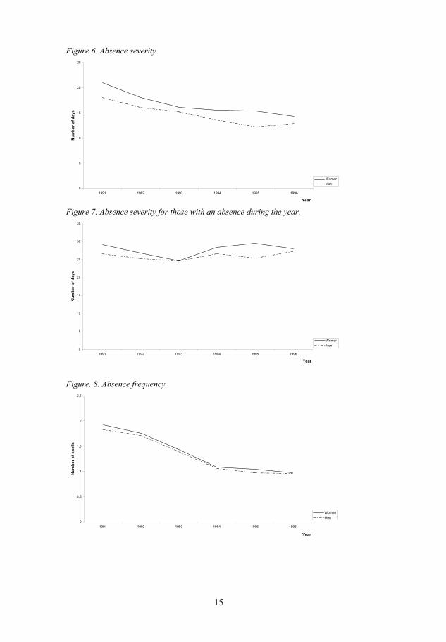
The absence frequency has declined during the whole period studied and the ab-sence frequency of women is just a little bit higher than the absence frequency of men (Figure 8). If we concentrate on the frequency of 1-day absences, there is a marked drop in 1993 when the qualification day was introduced (Figure 9). The frequency of medical absences also shows a decreasing trend during the 1990’s (Figure 10 and 11). Men and women tend to have the same frequency of short medical absence, but women seem to have a somewhat higher average frequency of long medical absence than men.

––––––––– 14 For men, the share that had no absence at all was in the range 32%–53%. For women, the share

was in the range 28%–49%.

14

15

Figure 6. Absence severity.

0

5

10

15

20

25

1991 1992 1993 1994 1995 1996

Year

Nu

mb

er

of

da

ys

Women

Men

Figure 7. Absence severity for those with an absence during the year.

0

5

10

15

20

25

30

35

1991 1992 1993 1994 1995 1996

Year

Nu

mb

er

of

da

ys

Women

Men

Figure. 8. Absence frequency.

0

0,5

1

1,5

2

2,5

1991 1992 1993 1994 1995 1996

Year

Nu

mb

er

of

sp

ell

s

Women

Men

15

16

Figure 9. Average frequency of attitudinal absence.

0

0,1

0,2

0,3

0,4

0,5

0,6

0,7

1991 1992 1993 1994 1995 1996

Year

Nu

mb

er

of

sp

ell

s

Women

Men

Figure 10. Average frequency of short medical absence.

0

0,1

0,2

0,3

0,4

0,5

0,6

1991 1992 1993 1994 1995 1996

Year

Nu

mb

er

of

sp

ell

s

Women

Men

Figure 11. Average frequency of long medical absence.

0

0,05

0,1

0,15

0,2

0,25

0,3

0,35

0,4

0,45

1991 1992 1993 1994 1995 1996

Year

Nu

mb

er

of

sp

ell

s

Women

Men

16

17

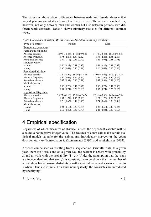
The diagrams above show differences between male and female absence that vary depending on what measure of absence is used. The absence levels differ, however, not only between men and women but also between persons with dif-ferent work contracts. Table 4 shows summary statistics for different contract types.

Table 4. Summary statistics. Means with standard deviations in parentheses.

Type of contract Women Men Temporary contracts/ Permanent contracts Absence severity 12.93 (32.85) / 17.98 (49.88) 11.10 (32.45) / 15.78 (46.88) Absence frequency 1.75 (2.29) / 1.37 (2.12) 1.53 (2.21) / 1.35 (2.13) Attitudinal absence 0.57 (1.12) / 0.39 (0.92) 0.46 (0.98) / 0.38 (0.98) Medical absence: - short 0.46 (0.87) / 0.38 (0.82) 0.41 (0.86) / 0.39 (0.83) - long 0.30 (0.67) / 0.30 (0.71) 0.26 (0.69) / 0.27 (0.67) Part-time/Full-time Absence severity 18.38 (51.96) / 16.36 (44.44) 17.00 (48.62) / 14.33 (43.47) Absence frequency 1.49 (2.02) / 1.40 (2.24) 1.47 (1.99) / 1.35 (2.19) Attitudinal absence 0.43 (0.94) / 0.40 (0.98) 0.43 (0.91) / 0.38 (1.00) Medical absence: - short 0.36 (0.76) / 0.41 (0.87) 0.36 (0.75) / 0.41 (0.86) - long 0.34 (0.74) / 0.28 (0.68) 0.33 (0.74) / 0.25 (0.65) Night-time/Day-time Absence severity 28.77 (61.10) / 17.08 (47.47) 17.51 (47.96) / 14.94 (44.75) Absence frequency 1.37 (1.71) / 1.43 (2.16) 1.27 (1.70) / 1.38 (2.15) Attitudinal absence 0.28 (0.62) / 0.42 (0.96) 0.24 (0.61) / 0.39 (0.99) Medical absence: - short 0.24 (0.57) / 0.39 (0.83) 0.32 (0.66) / 0.40 (0.84) - long 0.52 (0.89) / 0.30 (0.70) 0.41 (0.83) / 0.27 (0.67)

4 Empirical specification

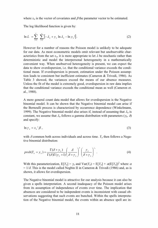
Regardless of which measures of absence is used, the dependent variable will be a count; a nonnegative integer value. The features of count data make certain sta-tistical models suitable for the estimations. Introductory surveys of the count data literature are Winkelmann & Zimmermann (1995) and Winkelmann (2003).

Absence can be seen as resulting from a sequence of Bernoulli trials. In a given year, there are n trials and on a given day, the worker is absent with probability pi and at work with the probability (1 - pi). Under the assumption that the trials are independent and that pi= it/n is constant, it can be shown that the number of absent days has a Poisson distribution with expected value and variance equal to

when n tends to infinity. To ensure nonnegativity, the covariates are introduced by specifying:

'lnitit

x , (1)

17

18

where xit is the vector of covariates and the parameter vector to be estimated.

The log likelihood function is given by:

n

i

itititit

T

t

yyL11

!lnlnln . (2)

However for a number of reasons the Poisson model is unlikely to be adequate for our data. As most econometric models omit relevant but unobservable char-acteristics from the set xit, it is more appropriate to let be stochastic rather than deterministic and model the interpersonal heterogeneity in a mathematically convenient way. When unobserved heterogeneity is present, we can expect the data to show overdispersion, i.e. that the conditional variance exceeds the condi-tional mean. If overdispersion is present, estimation under the Poisson assump-tion leads to consistent but inefficient estimates (Cameron & Trivedi, 1986). As Table 3 showed, the variances exceed the means of our absence measures. Unless the fit of the model is extremely good, overdispersion in raw data implies that the conditional variance exceeds the conditional mean as well (Cameron et. al., 1988).

A more general count data model that allows for overdispersion is the Negative binomial model. It can be shown that the Negative binomial model can arise if the Bernoulli process is characterized by occurrence dependence (Winkelmann, 1999). The Negative binomial model also arises if, instead of assuming that it is constant, we assume that it follows a gamma distribution with parameters ( it, )and specify:

'lnitit

x , (3)

with common both across individuals and across time. Yit then follows a Nega-tive binomial distribution:

ity

it

it

itit

it

itity

yyYprob

)1()(

)()( . (4)

With this parameterization, E[Yit] = it and Var(Yit) = E[Yit] + (E[Yit])2 where

= 1/ . This is the model called Negbin II in Cameron & Trivedi (1986) and, as is shown, it allows for overdispersion.

The Negative binomial model is attractive for our analysis because it can also be given a spells interpretation. A second inadequacy of the Poisson model arises from its assumption of independence of events over time. The implication that absences are considered to be independent events is inconsistent with casual ob-servations suggesting that such events are bunched. Within the spells interpreta-tion of the Negative binomial model, the events within an absence spell are in-

18

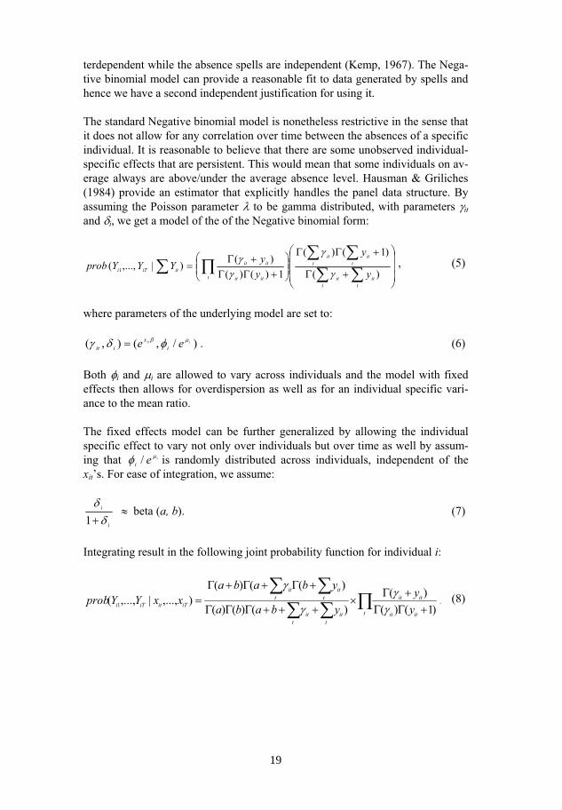
terdependent while the absence spells are independent (Kemp, 1967). The Nega-tive binomial model can provide a reasonable fit to data generated by spells and hence we have a second independent justification for using it.

The standard Negative binomial model is nonetheless restrictive in the sense that it does not allow for any correlation over time between the absences of a specific individual. It is reasonable to believe that there are some unobserved individual-specific effects that are persistent. This would mean that some individuals on av-erage always are above/under the average absence level. Hausman & Griliches (1984) provide an estimator that explicitly handles the panel data structure. By assuming the Poisson parameter to be gamma distributed, with parameters itand i, we get a model of the of the Negative binomial form:

t titit

t titit

t itit

itititiTi y

y

yyYYYprob

)(

)1()(

1)()()()|,...,( 1

, (5)

where parameters of the underlying model are set to:

)/,(),( iit ee ix

iit . (6)

Both i and i are allowed to vary across individuals and the model with fixed effects then allows for overdispersion as well as for an individual specific vari-ance to the mean ratio.

The fixed effects model can be further generalized by allowing the individual specific effect to vary not only over individuals but over time as well by assum-ing that iei / is randomly distributed across individuals, independent of the xit’s. For ease of integration, we assume:

i

i

1 beta (a, b). (7)

Integrating result in the following joint probability function for individual i:

t itit

itit

t titit

t titit

iTitiTi yy

ybaba

ybabaxxYYprob

)1()()(

)()()(

)(()(),...,|,...,( 1 . (8)

19

20

5 Results

We separate our analysis into two parts. First, we estimate a baseline model with only age, the reform dummies and unemployment as explanatory variables. We then add on the contract perspective and include not only the original variables, but also interactions between the reform dummies and the other contract vari-ables. This allows us to see whether the effects of the different reforms differ ac-cording to other aspects of the contract. Since earlier studies (VandenHeuvel & Wooden, 1995; Vistnes, 1997; Paringer, 1983) and our descriptive statistics show gender differences in absence, we estimate separate models for men and women.15

5.1 The baseline model

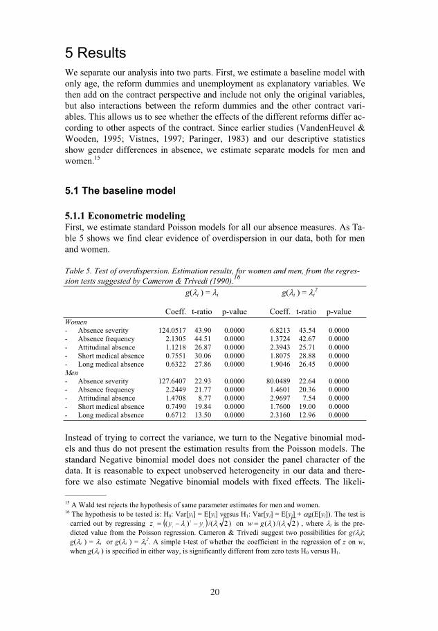
5.1.1 Econometric modeling First, we estimate standard Poisson models for all our absence measures. As Ta-ble 5 shows we find clear evidence of overdispersion in our data, both for men and women.

Table 5. Test of overdispersion. Estimation results, for women and men, from the regres-

sion tests suggested by Cameron & Trivedi (1990).16

g( i ) = i g( i ) = i2

Coeff. t-ratio p-value Coeff. t-ratio p-value Women

- Absence severity 124.0517 43.90 0.0000 6.8213 43.54 0.0000 - Absence frequency 2.1305 44.51 0.0000 1.3724 42.67 0.0000 - Attitudinal absence 1.1218 26.87 0.0000 2.3943 25.71 0.0000 - Short medical absence 0.7551 30.06 0.0000 1.8075 28.88 0.0000 - Long medical absence 0.6322 27.86 0.0000 1.9046 26.45 0.0000 Men

- Absence severity 127.6407 22.93 0.0000 80.0489 22.64 0.0000 - Absence frequency 2.2449 21.77 0.0000 1.4601 20.36 0.0000 - Attitudinal absence 1.4708 8.77 0.0000 2.9697 7.54 0.0000 - Short medical absence 0.7490 19.84 0.0000 1.7600 19.00 0.0000 - Long medical absence 0.6712 13.50 0.0000 2.3160 12.96 0.0000

Instead of trying to correct the variance, we turn to the Negative binomial mod-els and thus do not present the estimation results from the Poisson models. The standard Negative binomial model does not consider the panel character of the data. It is reasonable to expect unobserved heterogeneity in our data and there-fore we also estimate Negative binomial models with fixed effects. The likeli-

––––––––– 15 A Wald test rejects the hypothesis of same parameter estimates for men and women. 16 The hypothesis to be tested is: H0: Var[yi] = E[yi] versus H1: Var[yi] = E[yi] + g(E[yi]). The test is

carried out by regressing )2/()( 2

iiiiiyyz on )2/()(

iigw , where i is the pre-

dicted value from the Poisson regression. Cameron & Trivedi suggest two possibilities for g( i);g( i ) = i or g( i ) = i

2. A simple t-test of whether the coefficient in the regression of z on w,when g( i ) is specified in either way, is significantly different from zero tests H0 versus H1.

20

21

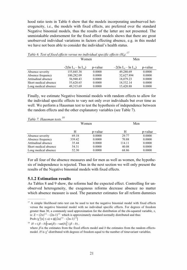
hood ratio tests in Table 6 show that the models incorporating unobserved het-erogeneity, i.e., the models with fixed effects, are preferred over the standard Negative binomial models, thus the results of the latter are not presented. The unmistakable endorsement for the fixed effect models shows that there are great unobserved individual variations in factors effecting absence, e.g. in this model we have not been able to consider the individual’s health status.

Table 6. Test of fixed effects versus no individual specific effects (H0).17

Women Men

-2(ln Lr – ln Lu) p-value –2(ln Lr – ln Lu) p-valueAbsence severity 155,845.38 0.0000 49,280.69 0.0000 Absence frequency 100,282.09 0.0000 32,627.894 0.0000 Attitudinal absence 56,940.43 0.0000 18,079.23 0.0000 Short medical absence 55,628.65 0.0000 18,532.14 0.0000 Long medical absence 49,315.69 0.0000 15,420.88 0.0000

Finally, we estimate Negative binomial models with random effects to allow for the individual specific effects to vary not only over individuals but over time as well. We perform a Hausman test to test the hypothesis of independence between the random effects and the other explanatory variables (see Table 7).

Table 7. Hausman tests.18

Women Men

H p-value H p-value Absence severity 69.18 0.0000 29.77 0.0000 Absence frequency 339.42 0.0000 70.88 0.0000 Attitudinal absence 35.44 0.0000 114.11 0.0000 Short medical absence 54.31 0.0000 40.08 0.0000 Long medical absence 52.30 0.0000 68.86 0.0000

For all four of the absence measures and for men as well as women, the hypothe-sis of independence is rejected. Thus in the next section we will only present the results of the Negative binomial models with fixed effects.

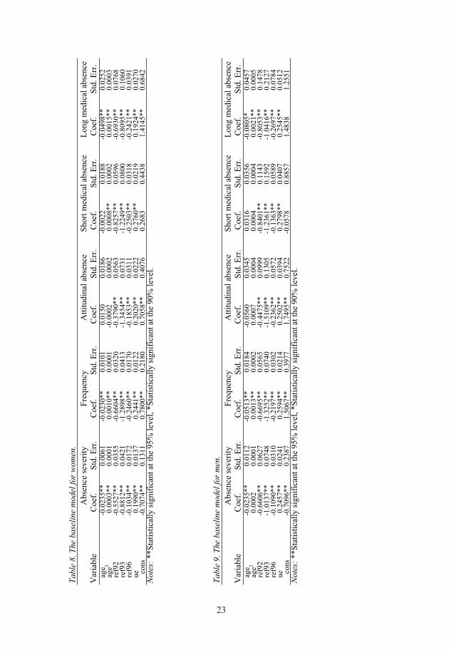
5.1.2 Estimation results As Tables 8 and 9 show, the reforms had the expected effect. Controlling for un-observed heterogeneity, the exogenous reforms decrease absence no matter which absence measure is used. The parameter estimates for all reform dummies

––––––––– 17 A simple likelihood ratio test can be used to test the negative binomial model with fixed effects

versus the negative binomial model with no individual specific effects. For degrees of freedom greater than 30, a commonly used approximation for the distribution of the chi-squared variable, x,is: Z = (2x)1/2 – (2n-1)1/2 which is approximately standard normally distributed and thus Prob ( 2[n] a) [(2a)1/2 – (2n-1)1/2]

18 )()var()var()(1

bbbH ,

where is the estimates from the fixed effects model and b the estimates from the random effects-model. H is 2-distributed with degrees of freedom equal to the number of timevariant variables.

21

22

are strongly significant for all absence measures. Despite the strong significance, some caution is recommended in evaluating the results. Three reforms in six years means that obtaining accurate estimates of the effects of the separate re-forms can be difficult (also discussed in Henrekson & Persson, 2004). It might rather be the case that the reform dummies together with the variable for the un-employment rate measure some other kind of a time factor. To be able to inter-pret the results we have to make the assumption that the only thing that changes over time is the sickness insurance system and the unemployment rate, i.e. that there are no other time factors that affect absence.19

To ensure that the reform dummies not only measure a time factor indicating that those workers with high rates of absence are those leaving the organization, we made a re-estimation only including those who remain in the organization for the entire period studied. We still obtain a clearly significant negative effect of the reforms on all absence measures. Our results are a reinforcement of the findings in Henrekson & Persson (2004). They also found a significant negative effect of the reforms that made the sickness insurance system more austere. Notably, all of the reforms also affect long medical absence. The explanation for this may be that the reforms imply cost increases for returning to work due to the possibility of returning to a new absence spell (Johansson & Palme, 2003).

In contrast to studies made on grouped data, we found a significant positive rela-tion between absence and the unemployment rate. Such a positive relation was also found in Johansson & Palme (2002). In our re-estimation of the models for only those employed in the organization for the entire period studied, we still ob-tain a significant positive effect of unemployment. This weakens the explanation for a counter-cyclical relation between absence and unemployment based on dis-cipline effects. Theorell et al. (2004) wrote that cuts in organizations have been found to increase illness. In the public health care organization in focus for our study, the beginning of the 1990’s was characterized by major cuts. It is possible that the unemployment rate variable serves as an indicator of the cuts and there-fore shows a positive relation to absence.

––––––––– 19 We have tried estimations with several different combinations of reform dummies without obtain-

ing any major differences in the estimates of the other parameters.

22

Table

8.

The

base

line

model

for

wom

en.

Abs

ence

sev

erit

y

Fre

quen

cy

A

ttit

udin

al a

bsen

ce

S

hort

med

ical

abs

ence

L

ong

med

ical

abs

ence

Var

iabl

e

Coe

f.

S

td. E

rr.

Coe

f.

Std

. Err

. C

oef.

S

td. E

rr.

C

oef.

S

td. E

rr.

Coe

f.

S

td. E

rr.

age

-0

.023

5**

0.00

61

-0

.023

0**

0.

0101

0.01

50

0.

0186

-

0.00

22

0.

0188

-

0.04

98**

0.02

52

ag

e2

0.00

03**

0.

0001

0.00

10**

0.00

01

-0

.000

2

0.00

02

0.

0008

**

0.

0002

0.00

15**

0.00

03

ref9

2-0

.552

7**

0.03

55

-0

.660

4**

0.

0320

-0.3

790*

*

0.0

563

-0

.825

7**

0.

0596

-0.6

930*

*

0.07

68

re

f93

-0.8

812*

* 0.

0421

-1.2

898*

*

0.04

13

-1

.345

4**

0.

0731

-1.2

249*

*

0.08

00

-0

.809

5**

0.

1060

ref9

6-0

.103

4**

0.01

72

-0

.246

0**

0.

0170

-0.1

853*

*

0.03

11

-0

.250

3**

0.

0318

-0.2

421*

*

0.03

91

ue

0.19

90**

0.

0137

0.2

441*

*

0.01

22

0.

2020

**

0.02

22

0.

2760

**

0.

0219

0.19

24**

0.

0270

_con

s

-0.7

074*

* 0.

1311

0.78

00**

0.21

80

0.

7058

**

0.4

076

0.26

83

0.

4438

1.41

45**

0.68

42

Note

s: *

*Sta

tist

ical

ly s

igni

fica

nt a

t the

95%

lev

el, *

Sta

tist

ical

ly s

igni

fica

nt a

t th

e 90

% l

evel

.

Table

9.

The

base

line

model

for

men

.

Abs

ence

sev

erit

y

Fre

quen

cy

A

ttit

udin

al a

bsen

ce

S

hort

med

ical

abs

ence

L

ong

med

ical

abs

ence

Var

iabl

e

Coe

f.

S

td. E

rr.

Coe

f.

Std

. Err

. C

oef.

S

td. E

rr.

C

oef.

S

td. E

rr.

Coe

f.

S

td. E

rr.

ag

e

-0.

0235

**

0.

0112

-0.0

513*

*

0.01

84

-0

.056

0

0.03

45

0.0

316

0.

0356

-0.0

805*

0.04

57

ag

e2

0.0

002

0.

0001

0.00

13**

0.00

02

0.

0007

0.00

04

0.

0004

0.00

04

0.

0021

**

0.

0005

ref9

2 -

0.66

06**

0.06

27

-0

.669

5**

0.

0565

-0.4

475*

*

0.09

99

-0.8

401*

*

0.11

43

-0

.805

3**

0.

1478

ref9

3

-1.

0137

**

0.

0748

-1.3

252*

*

0.07

40

-1

.510

9**

0.

1305

-1

.236

1**

0.

1592

-1.0

416*

*

0.21

27

re

f96

-

0.10

90**

0.03

10

-0

.219

7**

0.

0302

-0.2

362*

*

0.05

72

-0.1

363*

*

0.05

89

-0

.269

7**

0.

0784

ue

0.2

457*

*

0.02

41

0.

2594

**

0.

0214

0.25

02**

0.03

94

0.

2798

**

0.

0407

0.

2545

**

0.

0512

_con

s

-0.

7096

**

0.

2387

1.50

67**

0.39

77

1.

7495

**

0.

7522

-0

.057

8

0.88

57

1.

4838

1.25

51

Note

s: *

*Sta

tist

ical

ly s

igni

fica

nt a

t the

95%

lev

el, *

Sta

tist

ical

ly s

igni

fica

nt a

t th

e 90

% l

evel

.

23

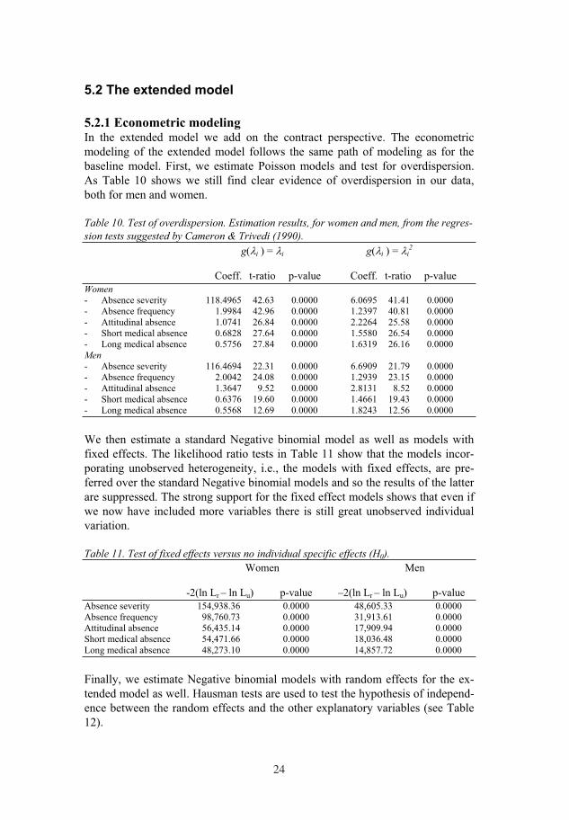
24

5.2 The extended model

5.2.1 Econometric modeling In the extended model we add on the contract perspective. The econometric modeling of the extended model follows the same path of modeling as for the baseline model. First, we estimate Poisson models and test for overdispersion. As Table 10 shows we still find clear evidence of overdispersion in our data, both for men and women.


sion tests suggested by Cameron & Trivedi (1990).

g( i ) = i g( i ) = i2

Coeff. t-ratio p-value Coeff. t-ratio p-value Women

- Absence severity 118.4965 42.63 0.0000 6.0695 41.41 0.0000 - Absence frequency 1.9984 42.96 0.0000 1.2397 40.81 0.0000 - Attitudinal absence 1.0741 26.84 0.0000 2.2264 25.58 0.0000 - Short medical absence 0.6828 27.64 0.0000 1.5580 26.54 0.0000 - Long medical absence 0.5756 27.84 0.0000 1.6319 26.16 0.0000 Men

- Absence severity 116.4694 22.31 0.0000 6.6909 21.79 0.0000 - Absence frequency 2.0042 24.08 0.0000 1.2939 23.15 0.0000 - Attitudinal absence 1.3647 9.52 0.0000 2.8131 8.52 0.0000 - Short medical absence 0.6376 19.60 0.0000 1.4661 19.43 0.0000 - Long medical absence 0.5568 12.69 0.0000 1.8243 12.56 0.0000

We then estimate a standard Negative binomial model as well as models with fixed effects. The likelihood ratio tests in Table 11 show that the models incor-porating unobserved heterogeneity, i.e., the models with fixed effects, are pre-ferred over the standard Negative binomial models and so the results of the latter are suppressed. The strong support for the fixed effect models shows that even if we now have included more variables there is still great unobserved individual variation.

Table 11. Test of fixed effects versus no individual specific effects (H0).

Women Men

-2(ln Lr – ln Lu) p-value –2(ln Lr – ln Lu) p-valueAbsence severity 154,938.36 0.0000 48,605.33 0.0000 Absence frequency 98,760.73 0.0000 31,913.61 0.0000 Attitudinal absence 56,435.14 0.0000 17,909.94 0.0000 Short medical absence 54,471.66 0.0000 18,036.48 0.0000 Long medical absence 48,273.10 0.0000 14,857.72 0.0000

Finally, we estimate Negative binomial models with random effects for the ex-tended model as well. Hausman tests are used to test the hypothesis of independ-ence between the random effects and the other explanatory variables (see Table 12).

24

25

Table 12. Hausman tests.

Women Men

H p-value H p-value Absence severity 281.47 0.0000 211.59 0.0000 Absence frequency 369.76 0.0000 100.46 0.0000 Attitudinal absence 125.85 0.0000 34.00 0.6104 Short medical absence 167.28 0.0000 75.45 0.0002 Long medical absence 155.01 0.0000 42.63 0.2416

For women, the hypothesis of independence is rejected for all five of the absence measures. For men, on the other hand, the hypothesis can only be rejected for ab-sence severity, absence frequency and short medical absence. In the following section, the results from the fixed effects model are presented for those absence measures where the hypothesis has been rejected. For the measures for which the hypothesis cannot be rejected, we present the results from the random effects models.

5.2.2 Estimation results For the fixed effects models, those individuals observed only once do not con-tribute to the estimates. Yet another drawback of using fixed effects specifica-tions is that the estimation algorithm excludes individuals whose dependent vari-able never changes. As such, those individuals who are never absent do not con-tribute to the likelihood function. The random effects specification does not suf-fer from these deficiencies but unfortunately we could only use such specifica-tions for some of the dependent variables due to the rejection of the hypothesis of independence. Unlike linear models, fixed effects Negative binomial models are conditioned on the individual heterogeneity rather than the individual mean, hence it is possible to get parameter estimates for time invariant variables. We can therefore include both a constant and time invariant variables in all our esti-mations.

The results, in Table 13 and 14, show interesting differences between the various absence measures. Workers with part-time contracts have higher absence fre-quency compared to full-time workers. Women working part-time also have higher attitudinal absence but, on the other hand, less absence severity. One pos-sible explanation for the relation between working part-time and absence is that individuals choose to work part-time because of other commitments, a situation correlated with a lower degree of loyalty to the work place. This might then re-sult in repeated absence spells.

Workers on temporary contracts are found to have higher absence, considering all measures except male short and female long medical absence, which is the same result found in Barmby & Treble (1989). This result contradicts the result of Arai & Skogman Thoursie (2005), who suggest that there is a discipline effect of temporary contracts. In the organization studied, many of the temporary con-tracts stem from leaves of absence due to pregnancy and taking care of small children. This means that the owner of the contract knows for certain that the

25

26

contract will end, which may imply less loyalty. Shapiro & Stiglitz (1984, p. 436) writes, ”if one is going to have to leave the firm anyway, one might as well cheat on the firm”. Another possible explanation for higher absence among tem-porary workers might be if unhealthy workers were the ones receiving temporary contracts, i.e. some kind of selection effect. If there were such a selection effect, we would expect to find more long medical absences among temporary workers. This is only the case for men in our analysis.

It is also interesting to note that women working at night have less attitudinal ab-sence and more long medical absence. The latter could probably be explained by the poorer health often present with persons working nighttime. Nighttime work-ers having less attitudinal absence might have to do with less need for using ab-sence as a flexibility device. Working nighttime involves working fewer nights compared to the number of days a daytime worker works. In other words, night-time workers are more often off work compared to their daytime colleagues.

The age pattern seems to be about the same for both men and women. The effect is non-linear and the pattern begins with decreasing absence, but after reaching a certain age absence starts to increase. For female absence frequency and male long medical absence, the path turns early and absence increases with age. For female attitudinal absence and male absence severity we find no significant age effects.

When we add the contract perspective, the sign of the unemployment parameter estimate changes for both male and female attitudinal absence and female ab-sence frequency but not for the other absence measures. If we re-estimate the ex-tended model for just those who are employed the whole period we do not get this sign change. Thus, our findings do not support the disciplining effect as an explanation of a negative relation between unemployment and absence.

We can see from the tables that the exogenous reforms affected absence differ-ently depending on other contract characteristics. For women, for example, ab-sence severity declined more for those with temporary contracts after the reform in 1993 than for those with permanent contracts. Thus it seems that female tem-porary workers are more cost-sensitive than permanent workers, i.e. exhibit greater extent of moral hazard. For men we find a reversed relation. Men on tem-porary contracts are less cost-sensitive than men with permanent contracts. Male nighttime workers on the other hand seem to be more cost-sensitive than male daytime workers. We can see that after the reform in 1992, attitudinal absence increases for female temporary workers. This might be explained by a stronger absence control from the employer. Thus temporary workers only stay home for one day and then gets back to work in a greater extent than earlier. For men with temporary contracts, there is a decrease in long medial absence after the reform in 1992. This would be the result if the employer uses absence screening before prolonging the temporary contract.

26

27

Persons with different occupations also reacted differently to the reforms during the 1990’s. It seems, for example, that female cleaners, washers and transporta-tion personnel (occ4) are not as effected by the reforms as women with other oc-cupations. For all other occupations, absence severity declined significantly after the reforms in 1992, 1993 and 1996. After the reform of 1992, all occupations, except male doctors and male technicians, increased their attitudinal absence. In-creased attitudinal absence might reflect it being more important to show loyalty after the reform since the employers monitoring can be expected to have in-creased. When ill, workers only take one day off and then return to work. This is in line with earlier studies showing increased illness attendance at work during the 1990’s. Male doctors, however, are the only group of men for whom absence frequency decreased after the reform in 1992. Female doctors do not show the same pattern, though other groups of women do.

Finally, we can see that for all occupations, except for female technicians, both absence frequency and attitudinal absence decrease after the reform of 1993 where the qualification day was introduced. The many non-significant estimates for female technicians might have to do with few observations (524 in the total sample).

27

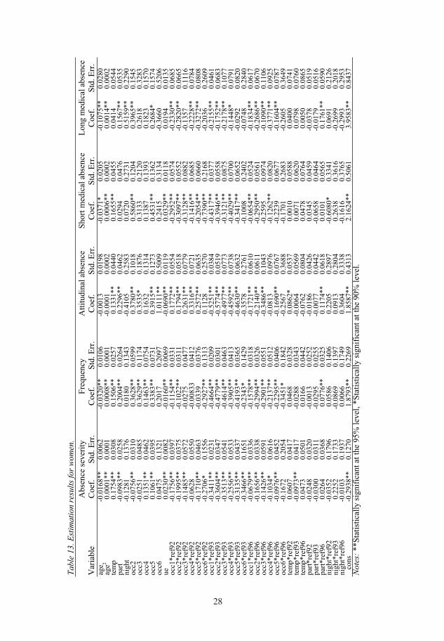
Table

13.E

stim

ati

on r

esult

s fo

r w

om

en.

Abs

ence

sev

erit

y

Fre

quen

cy

A

ttit

udin

al a

bsen

ce

S

hort

med

ical

abs

ence

L

ong

med

ical

abs

ence

Var

iabl

e

Coe

f.

S

td. E

rr.

Coe

f.

Std

. Err

. C

oef.

S

td. E

rr.

C

oef.

S

td. E

rr.

Coe

f.

S

td. E

rr.

age

-0

.016

8**

0.00

62

-0

.032

0**

0.

0106

-0.0

013

0.

0198

-0.0

371*

0.

0205

-0

.107

5**

0.

0280

ag

e2

0.0

001*

*

0.00

01

0.0

008*

*

0.00

01

-0

.000

1

0.00

02

0.

0006

**

0.00

02

0.00

14**

0.

0002

te

mp

0.17

54**

0.

0308

0.15

06**

0.02

57

0.

1331

**

0.04

40

0.

1655

**

0.04

55

0.04

14

0.05

44

part

-0

.098

3**

0.

0258

0.20

04**

0.02

64

0.

2296

**

0.04

62

0.

0294

0.

0476

0.

1567

**

0.05

35

nigh

t -

0.12

81

0.13

76

0.

0180

0.13

43

-0.4

105

0.

2583

0.07

20

0.27

31

0.51

59**

0.

2290

oc

c2-0

.075

6**

0.

0310

0.36

28**

0.05

99

0.37

80**

0.

1018

0.58

60**

0.

1204

0.

3965

**

0.15

45

occ3

-0.0

251

0.

0485

0.36

29**

0.11

74

0.35

35*

0.

1876

0.31

33

0.21

20

0.26

18

0.32

83

occ4

0.13

51**

0.

0462

0.14

63**

0.07

54

0.

1632

0.

1314

0.13

87

0.13

93

0.18

23

0.15

70

occ5

0.10

61**

0.

0395

0.33

83**

0.07

31

0.

3915

**

0.12

73

0.

4531

**

0.13

62

0.26

84*

0.

1574

oc

c60.

0475

0.

1321

0.20

17

0.

2097

1.01

11**

0.

5009

0.24

15

0.31

34

-0.3

660

0.

5206

ue

0

.023

0**

0.

0082

-0.0

160*

*

0.00

69

-0.0

690*

*

0.01

19

0.

0329

**

0.01

18

0.01

94

0.01

35

occ1

*ref

92

-0.

1756

**

0.03

97

-0

.115

4**

0.

0331

0.17

72**

0.

0554

-0.2

952*

*

0.05

74

-0.2

330*

*

0.06

85

occ2

*ref

92

-0.1

995*

*

0.03

75

-0

.102

2**

0.

0311

0.17

94**

0.

0518

-0.3

097*

*

0.05

52

-0.2

820*

*

0.06

65

occ3

*ref

92

-0

.148

5**

0.

0572

-0.0

275

0.

0477

0.

2631

**

0.07

79

-0

.312

8**

0.

0882

-0

.135

7

0.11

16

occ4

*ref

92

-0

.062

8

0.05

50

-0

.008

33

0.04

12

0.

3316

**

0.07

21

-0

.141

6**

0.

0685

-0

.222

8**

0.

0784

oc

c5*r

ef92

-0

.171

0**

0.

0463

-0.0

339

0.

0376

0.

2572

**

0.06

35

-0

.205

4**

0.

0660

-0

.327

2**

0.

0808

oc

c6*r

ef92

-0

.270

6*

0.15

56

-0

.292

7**

0.

1313

0.

1128

0.

2570

-0.7

390*

*

0.21

68

-0.2

036

0.

2609

oc

c1*r

ef93

-0.3

411*

*

0.02

31

-0

.466

4**

0.

0209

-0

.525

1**

0.

0384

-0

.431

7**

0.

0377

-0

.215

5**

0.

0461

oc

c2*r

ef93

-

0.36

04**

0.

0347

-0.4

779*

*

0.03

01

-0.5

774*

*

0.05

19

-0.3

946*

*

0.05

58

-0.1

752*

*

0.06

83

occ3

*ref

93

-0.

3513

**

0.05

41

-0

.461

4**

0.

0463

-0.4

977*

*

0.07

73

-0

.312

1**

0.

0875

-0

.217

8**

0.

1077

oc

c4*r

ef93

-

0.25

56**

0.

0533

-0.3

905*

*

0.04

13

-0.4

592*

*

0.07

38

-0

.402

9**

0.

0700

-0

.144

8*

0.07

91

occ5

*ref

93

-0.

3135

**

0.04

37

-0

.419

3**

0.

0365

-0

.463

0**

0.

0632

-0.3

417*

*

0.06

52

-0.0

292

0.

0820

oc

c6*r

ef93

-

0.34

66**

0.

1651

-0.2

343*

0.14

29

-0

.357

8

0.27

61

-0

.100

8

0.24

02

-0.0

748

0.

2840

oc

c1*r

ef96

-

0.06

79**

0.

0336

-0.1

578*

*

0.03

18

-0.1

721*

*

0.06

10

-0

.065

4**

0.

0524

-0

.183

4**

0.

0617

oc

c2*r

ef96

-0

.165

6**

0.

0338

-0

.299

4**

0.

0326

-0

.214

0**

0.

0611

-0.2

950*

*

0.05

61

-0.2

686*

*

0.06

70

occ3

*ref

96

-0.1

426*

*

0.05

91

-0

.290

1**

0.

0551

-0

.348

6**

0.

1043

-0.2

595

0.

0974

-0

.109

0**

0.

1106

oc

c4*r

ef96

-0

.103

4*

0.06

16

-0

.213

7**

0.

0512

-0

.081

3

0.09

76

-0.1

262*

*

0.08

20

-0.3

771*

*

0.09

25

occ5

*ref

96

-0.0

976*

*

0.04

52

-0

.229

5**

0.

0406

-0

.169

0**

0.

0767

-0

.223

9

0.06

77

-0.1

604*

*

0.07

87

occ6

*ref

96

-0.1

672

0.

2054

-0.3

451*

0.18

42

-0.2

567

0.

3688

-0

.170

1

0.26

83

-0.2

605

0.

3649

te

mp*

ref9

2 0

.060

7

0.04

17

0.

0468

0.03

28

0.

0862

*

0.05

37

0.

0010

0.

0588

0.

0400

0.

0741

te

mp*

ref9

3

-0.0

973*

*

0.04

17

-0

.028

8

0.03

43

-0.0

064

0.

0569

0.00

71

0.06

20

0.07

98

0.07

60

tem

p*re

f96

0.

0473

0.

0501

0.01

66

0.

0442

-0

.076

2

0.08

04

0.

0478

0.

0764

0.

0050

0.

0865

pa

rt*r

ef92

-0.0

248

0.

0320

-0.0

013

0.

0252

-0

.018

6

0.04

26

0.

0345

0.

0459

-0

.037

8

0.05

19

part

*ref

93

-0

.030

0

0.03

11

-0

.029

5

0.02

55

-0.0

077

0.

0442

-0.0

658

0.

0464

-0

.017

9

0.05

16

part

*ref

96

0.0

264

0.

0368

0.07

76**

0.

0325

0.

1174

**

0.06

18

0.

0101

0.

0565

0.

1761

**

0.05

90

nigh

t*re

f92

-0.0

352

0.

1796

0.

0586

0.14

06

0.22

05

0.28

97

-0

.608

0*

0.33

41

0.06

91

0.21

26

nigh

t*re

f93

0

.225

2

0.17

33

-0

.086

9

0.13

97

0.09

13

0.28

04

0.

2638

0.

3616

-0

.269

9

0.20

18

nigh

t*re

f96

-0

.010

3

0.19

37

0.

0066

0.17

49

0.36

04

0.33

38

-0

.161

6

0.37

65

-0.2

993

0.

2953

_

cons

-0.

2938

**

0.12

70

1.

8793

**

0.

2269

1.

8587

**

0.43

13

2.

1624

**

0.50

61

3.95

83**

0.

8437

N

ote

s: *

*Sta

tist

ical

ly s

igni

fica

nt a

t the

95%

lev

el, *

Sta

tist

ical

ly s

igni

fica

nt a

t th

e 90

% l

evel

.

28

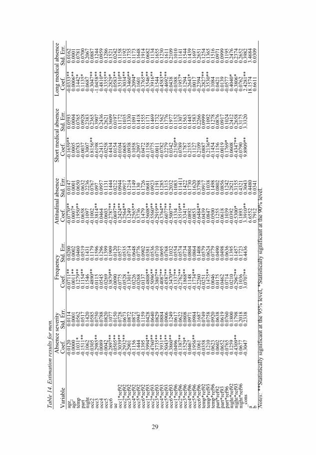
Table

14.E

stim

ati

on r

esult

s fo

r m

en.

Abs

ence

sev

erit

y

Fre

quen

cy

A

ttit

udin

al a

bsen

ce

S

hort

med

ical

abs

ence

L

ong

med

ical

abs

ence

V

aria

ble

C

oef.

Std

. Err

. C

oef.

S

td. E

rr.

Coe

f.

Std

. Err

.

Coe

f.

Std

. Err

. C

oef.

Std

. Err

. ag

e

-0.0

120

0.

0114

-0.0

711*

*

0.02

00

-0.

0770

**

0.01

47

-0.

1659

**

0.05

93

-0.

0333

**

0.

0162

ag

e2

0.0

000

0.

0001

0.00

11**

0.

0002

0.

0007

* 0.

0001

0.00

05

0.00

04

0.00

06**

0.00

01

tem

p

0.1

031*

0.

0562

0.12

79**

0.

0460

0.

1950

**

0.06

50

0.

0783

0.

0765

0.

1442

*

0.07

81

part

-0

.151

1**

0.

0517

0.11

54**

0.

0519

0.

0658

0.

0632

-0.0

037

0.

0928

0.

1135

*

0.07

00

nigh

t

-0.1

062

0.

1420

0.15

46

0.14

31

-0.1

097

0.

2236

0.30

07

0.23

83

0.06

87

0.

2067

oc

c2

-0.0

305

0.

0585

0.

4890

**

0.

1179

-0

.100

2

0.07

67

0.

8156

**

0.23

65

-0.3

047*

*

0.08

87

occ3

-0

.298

5**

0.

0750

-0

.011

5

0.15

96

-0.3

814*

*

0.09

7

-0.6

198

0.

3907

-1

.045

8**

0.

1244

oc

c4

0.0

089

0.

0788

0.

0545

0.

1296

0.

0464

0.

0957

-0

.241

3

0.24

36

0.48

10**

0.

0959

oc

c5

-0.0

042

0.

0820

-0

.026

9

0.13

99

-0.0

603

0.

1131

-0.0

258

0.

2621

-0

.335

5**

0.

1286

oc

c6

-0.2

897*

*

0.10

77

0.38

79**

0.

1909

-0

.278

7**

0.

1444

0.44

34

0.36

09

-0.2

829*

0.15

21

ue

0.0

505*

*

0.01

50

-0

.009

0

0.01

20

-0.0

697*

*

0.02

12

0.01

54

0.01

97

0.05

83**

0.02

42

occ1

*ref

92

-0.3

039*

*

0.07

28

-0

.077

5

0.05

77

0.24

24**

0.

0944

-0

.010

4

0.11

72

-0.3

510*

*

0.11

58

occ2

*ref

92

-0.

2932

**

0.06

73

-0

.052

8

0.05

35

0.25

64**

0.

0917

-0

.068

5

0.10

35

-0.3

034*

* 0.

1192

oc

c3*r

ef92

-0.2

901

0.

0872

-0.1

301*

0.

0714

0.

1249

0.

1214

-0

.093

8

0.13

30

-0.

3460

**

0.17

35

occ4

*ref

92

-0

.115

6

0.08

72

0.

0226

0.

0648

0.

2565

**

0.11

49

0.

1058

0.10

91

-0.2

094*

0.11

73

occ5

*ref

92

-0.1

444

0.

0947

-0.0

268

0.

0776

0.37

36

0.

130

-0

.209

7

0.14

18

-0.1

601

0.

1648

oc

c6*r

ef92

-0

.139

5

0.11

59

-0

.013

7

0.09

02

0.14

79

0.17

26

0.

0472

0.15

55

-0.3

765*

*

0.19

14

occ1

*ref

93

-0.3

994*

*

0.04

28

-0

.480

8**

0.

0381

-0

.560

8**

0.

0681

-0

.115

8

0.11

71

-0.3

546*

*

0.06

82

occ2

*ref

93

-0

.476

0**

0.

0640

-0.5

096*

*

0.05

36

-0.5

560*

*

0.09

23

-0.0

775

0.

1469

-0

.391

6**

0.

1134

oc

c3*r

ef93

-0.3

735*

*

0.08

29

-0

.380

7**

0.

0710

-0

.291

9**

0.

1191

-0

.001

1

0.17

32

-0.1

544

0.

1655

oc

c4*r

ef93

-0.3

931*

*

0.08

84

-0

.408

7**

0.

0695

-0

.376

4**

0.

1285

-0

.078

2

0.15

62

-0.4

583*

*

0.12

30

occ5

*ref

93

-

0.50

43**

0.

0906

-0.4

587*

*

0.07

68

-0.6

077*

*

0.13

15

0.

2279

0.

1776

-

0.46

92**

0.

1611

oc

c6*r

ef93

-0

.386

0**

0.

1249

-0.3

470*

*

0.10

32

-0.5

007*

*

0.20

32

0.

0342

0.

1977

-0

.043

8

0.21

09

occ1

*ref

96

-0

.049

6

0.06

17

-0

.133

7**

0.

0554

-0

.133

4

0.10

83

0.

2150

**

0.11

52

-0.0

388

0.

1010

oc

c2*r

ef96

-0.1

387*

*

0.06

22

-0

.276

2**

0.

0574

-0

.351

9**

0.

1141

1

0.07

89

0.13

07

-0.1

957*

0.11

41

occ3

*ref

96

-

0.15

29*

0.

0808

-0.1

868*

*

0.07

34

-0.3

341*

*

0.14

22

0.17

87

0.15

63

-0.1

294

0.

1544

oc

c4*r

ef96

0.0

467

0.

0971

-0.1

148

0.

0804

-0

.089

2

0.17

30

0.21

55

0.14

45

-0.2

643*

0.14

39

occ5

*ref

96

-0.1

956*

*

0.09

84

-0

.173

4**

0.

0864

-0

.085

3

0.16

20

0.11

27

0.15

83

0.00

17

0.

1697

oc

c6*r

ef96

-0.

1061

0.

1687

-0.2

260

0.

1408

-0

.648

4**

0.

3798

0.

2109

0.

2266

-0

.239

4

0.26

51

tem

p*re

f92

-

0.03

58

0.07

49

-0

.025

1

0.05

79

-0.0

439

0.

0917

-0

.088

7

0.09

99

-0.2

827*

*

0.12

54

tem

p*re

f93

0

.121

0

0.07

58

0.

1475

**

0.06

24

0.08

47

0.10

38

0.21

36**

0.

1092

0.

3530

**

0.

1365

te

mp*

ref9

6

0.0

623

0.

0920

0.00

46

0.07

79

-0.0

500

0.

1498

-0

.145

4

0.12

78

0.10

84

0.

1516

pa

rt*r

ef92

0

.060

2

0.06

38

0.

0175

0.

0490

0.

1255

0.

0802

-0

.115

6

0.08

76

0.04

21

0.

0971

pa

rt*r

ef93

-

0.06

52

0.06

19

-0

.046

2 0.

0498

-0

.061

8

0.08

56

-0.0

019

0.

0917

0

.013

9

0.09

99

part

*ref

96

-0

.076

5

0.07

60

0.

0714

0.

0636

0.

1039

0.

1242

0.

1769

*

0.10

24

-0.0

577

0.

1195

ni

ght*

ref9

2

0.1

259

0.

1800

0.02

10

0.13

95

-0.0

392

0.

2821

0.

0608

0.

2412

0.

4040

*

0.24

76

nigh

t*re

f93

-0

.430

9**

0.

1798

-0.2

967*

*

0.14

57

-0.5

300*

0.

3155

-0

.434

7**

0.

2658

-0

.380

6*

0.

2374

ni

ght*

ref9

6

0.

0677

0.

2018

0.10

36

0.17

23

0.18

93

0.43

21

-0.0

790

0.

3175

0

.076

2

0.26

52

_co

ns

-0

.304

7

0.23

38

3.

0707

**

0.44

36

3.

3910

**

0.30

43

9.89

09**

3.

3320

2.

4281

**

0.39

82

a

6.

6552

0.

4480

18

.157

4

3.46

84

b

0.

7912

0.

0341

0.66

11

0.03

09

Note

s: *

*Sta

tist

ical

ly s

igni

fica

nt a

t the

95%

lev

el, *

Sta

tist

ical

ly s

igni

fica

nt a

t th

e 90

% l

evel

.

29

30

6 Conclusions

There are three main conclusions from this study. First, we find presence of moral hazard in the Swedish sickness insurance system. The reforms of 1993 and 1996 increased the cost of absence for the workers and we find significant nega-tive effects on all absence measures of these reforms. We thus obtain the same result as Henrekson & Persson (2004), i.e., a more austere insurance system re-duces absence. Not only workers exhibit moral hazard, so do the employers. The reform of 1992 (where the responsibility for sick pay was transferred to the em-ployers) had the desired effect - it decreased absence. This can probably be ex-plained by increased monitoring rather than improvements in work environment.

Second, our expectations about differences in the relation between absence and work contract characteristics, depending on what measure of absence is used, turn out to be valid. For example, we found that women working part-time have less absence when measured as the total number of absent days per year. When we instead analyzed the total number of absence spells we found that they are more frequent for men and women working part-time than for full-time workers. These results show how important it is to be observant of what measures of ab-sence are actually used in different studies. Differences in comparisons of earlier studies may sometimes just be due to different absence measures having been used.

The reforms of the sickness benefit system should actually be seen as changes in the work contract. Our third conclusion is that these changes affected work ab-sence differently depending on other contract characteristics, i.e. moral hazard differs depending on work contract structure. We found for example, that work-ers with certain occupations were less cost-sensitive than others. We also found gender differences in this respect. Absence severity for male nighttime workers decreased more after the reform of 1993 than it did for daytime workers. For women, we found no such significant difference. Absence severity decreased more for women with temporary contracts compared to those with permanent contracts. For men on the other hand, absence severity fell less for temporary workers than for permanent workers. Our estimations showed that also the re-form of 1992 affected some groups different from others. Cleaners, washers and transportation personnel seem not to have been affected at all, while male doc-tors are the only ones with reduced absence frequency as a result of the reform. Female temporary workers increased their one-day absences while male tempo-rary workers had less long medical absence after the reform in 1992. The de-creases in some absence measures and the increases in others can probably be in-terpreted as resulting from increased use of absence monitoring and screening by the employer. The increased costs of absence for the employers give them incen-tives to use screening of presumptive workers. Our results show that this proba-bly has affected the absence behavior of workers with temporary contracts.

30

31

The working situation deteriorated during the 1990’s, primarily due to staff cut-backs. From 1991 to 1996 the number of employees was reduced from over 23,000 to around 14,000 and workplace stress increased. Increased monitoring by employers is found to decrease absence, but monitoring by other workers in the work group, i.e. what Gellalty (1995) called social or group monitoring, would give the same result. The reduced number of workers might have led to stronger social monitoring alongside the increased monitoring by the employers.

31

32

ReferencesArai, M & Skogman Thoursie, P (2005). “Incentives and Selection in Cyclical Absentee-

ism”. Labour Economics, vol 12 issue 2, p 269-280.

Barmby, T A & Treble, J G (1989). “A Note on Absenteeism”. British Journal of Indus-trial Relations. vol 27:1, p 155-158.

Barmby, T, Orme, C & Treble, J (1991). “Worker absenteeism: an analysis using micro-data”. The Economic Journal, vol 101, p 214-229.

Barmby, T, Orme, C & Treble, J B (1995). “Worker absence histories: a panel study”. Labour Economics, 2, p 53-65.

Björklund, A (1991). “Vem får sjukpenning? En empirisk analys av sjukfrånvarons be-stämningsfaktorer”. I Arbetskraft, arbetsmarknad och produktivitet, Expertrapport nr 4 till Produktivitetsdelegationen.

Brown, S & Sessions, J G (1994). The Economics of Absence: Theory and Evidence. De-partment of Economics, Loughborough University of Technology, Leicestershire, Eng-land.

Bäckman, O (1992). “Abetslöshet och sjukfrånvaro - samband eller skensamband?”. So-

ciologisk Forskning, nr 4, p 38-49.

Bäckman, O (1998). Longitudinal Studies on Sickness Absence in Sweden. Swedish Insi-tute for Social Research, Dissertation Series, no 34.



Cameron, A C, Trivedi, P K, Milne, F and Piggott, J (1988) “A Microeconometric Model of the Demand for Health Care and Health Insurance in Australia”. The Review of Economic Studies, vol 55, issue 1, p 85-106.

Cameron, A C & Trivedi, P K (1990). “Regression based tests for overdispersion in the Poisson Model”. Journal of Econometrics, no 46, p 341-364.

Chaudhury, M & Ng, I (1992). “Asenteeism predictors: least squares, rank regression, and del selection results”. Canadian Journal of Economics, no 3, p 615-635.

Dagens Medicin (1999). “Kroppstemperaturen avslöjar patienternas sömnproblem”. 19990601, Stockholm.

Dagens Medicin (2000). “Ökad risk för arbetsskador och hjärtsjukdomar bland nattjobba-re”. 20000516, Stockholm.

Drago, R & Wooden, M (1992). “The determinants of labor absence: Economic factors and work group norms across countries”. Industrial and Labor Relations Review, vol 45, p 764-778.

32

33

Dunn, L F & Youngblood S A (1986). “Absenteeism as a Mechanism for Approaching an Optimal Labor Market Equilibrium: An Empirical Study”. The Review of Economics and Statistics, vol 68, no 4, p 668-674.

Edgerton, D, Kruse, A, & Wells, C (1996). Besparingsåtgärder på socialförsäkringsom-

rådet. En utvärdering av förändringar i sjukpenningförsäkringen. Slutrapport till Riksdagens Revisorer, 1996-09-13, Stockholm.

Gellalty, I R (1995). “Individual and group determinants of employee absenteeism: test of a causal model”. Journal of organizational behavior, vol 16, p 469-485.

Hausman, J, Hall, B H & Griliches, Z (1984). “Econometric models for count data with an application to the patents-R&D relationship”. Econometrica, vol 52, no 4, p 909-938.

Henrekson, J, Lantto, K & Persson, M (1992). Bruk och missbruk av sjukförsäkringen.SNS Förlag.


Hetzler, A & Eriksson, K E (1991). Den ersatta sjukfrånvaron: en studie av sjukskriv-

ningsmönstret. Studier i välfärdssamhälle, socialförsäkring och arbetsliv, Bokbox, Lund.

Högstedt, C et al. (red) (2004). Den höga sjukfrånvaron – sanning och konsekvens. Sta-tens folkhälsoinstitut, Stockholm.


nomics, vol 30, p 1493-1503.



Johansson, P & Palme, M (2003). Moral hazard and sickness insurance: Empirical evi-

dence from a sickness insurance reform in Sweden. Working paper 2004:10, IFAU In-stitute for Labour Market Policy Evaluation, Uppsala. Forthcoming in Journal of Pub-lic Economics.

Kemp, C D (1967). “On a contagious distribution suggested for accident data”. Biomet-rics, vol 23, no 2 (june), p 241-55.

Lantto, K (1991). Optimal Deterrents to Malingerence. Ph.D. Thesis, Department of Eco-nomics, Stockholm University.

Leigh, J P (1985). “The effects of Unemployment and the Business Cycle on Absentee-ism”. Journal of Economics and Business, vol 37:2, p 159-171.

Mathieu, J & Kohler, S (1990). “A Cross-Level Examination of Group Absence Influ-ences on Individual Absence”. Journal of Applied Psychology, vol 75, no 2, p 217-220.

33

34

Palmer, E (2003). “Svensk sjukskrivning i ett internationellt perspektiv” in Swedenborg, B (red) Varför är svenskarna så sjuka?, SNS Förlag, Stockholm.

Paringer, L (1983). “Women and Absenteeism: Health or Economics”. The American Economic Review, Papers and Proceedings of the Ninety-Fifth Annual Meeting of the American Economic Association, New York, New York, December 29-30, 1982, p 123-27.

Prop 1990/91:181: Regeringens proposition 1990/91:181 om sjuklön, m.m.

RFV (1995). Socialförsäkringsstatistik. Fakta 1995. Riksförsäkringsverket, Stockholm.


Rosen, S (1986). “The theory of equalizing differences” in Ashenfelter, O & Layard, R. (ed) Handbook of Labor Economics, vol 1, p 641-692, North Holland, Amsterdam.

Scott, K D & McClelland, E L (1990). “Gender differences in absenteeism”. Public Per-sonnel Management, vol 19, no 2, p 229-253.

Shapiro, C & Stiglitz, J E (1984). “Equilibrium unemployment as a worker discipline de-vice”. The American Economic Review, vol 77, p 433-444.

Theorell, T, Oxenstierna, G & Westerlund, H (2004). “Ju färre vi är tillsammans... sjuk-skrivningsmönster vid strukturella förändringar” i Högstedt et al. Den höga sjukfrån-varon – sanning och konsekvens. Folkhälsoinstitutet, Stockholm.

VandenHeuvel, A & Wooden, M (1995). “Do explanations of absenteeism differ for men and women?”. Human Relations, vol 48, no 11, p 1309-1329.

Vistnes, J P (1997). “Gender differences in days lost from work due to illness”. Industrial and Labor Relations Review, vol 50, no 2, p 304-323.

Vogel, J, Kindlund, H & Diderichsen, F (1992). Arbetsförhållanden, ohälsa och sjukfrån-

varo 1975-1989. SCB Levnadsförhållanden, rapport nr. 78.

Winkelmann, R (1999). “Wages, firm size and absenteeism”. Applied Economics Letters,vol 6, p 337-341.

Winkelmann, R (2003). Econometric Analysis of Count Data. 4 ed., Springer, Berlin.

Winkelmann, R & Zimmermann K.F (1995). “Recent developments in count data model-ing: theory and application”. Journal of Economic Surveys, vol 9, p 1-24.

Östlin, P et al. (1996). Kön och ohälsa - en antologi om könsskillnader ur ett folkhälso-perspektiv. Studentlitteratur, Lund.

34

Essay II

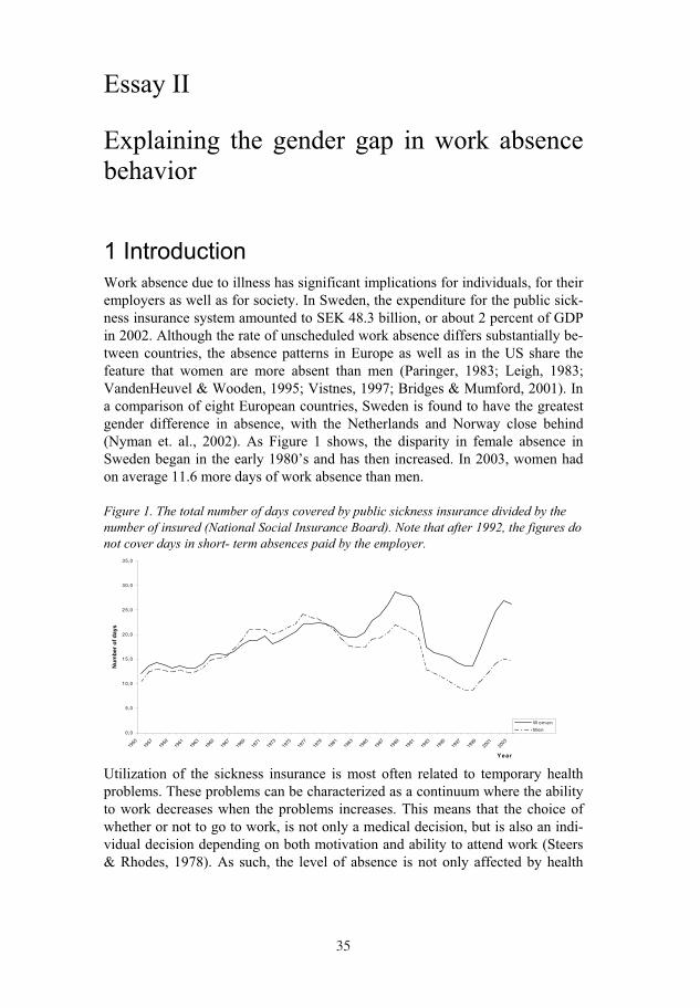
35

Essay II

Explaining the gender gap in work absence behavior

1 Introduction

Work absence due to illness has significant implications for individuals, for their employers as well as for society. In Sweden, the expenditure for the public sick-ness insurance system amounted to SEK 48.3 billion, or about 2 percent of GDP in 2002. Although the rate of unscheduled work absence differs substantially be-tween countries, the absence patterns in Europe as well as in the US share the feature that women are more absent than men (Paringer, 1983; Leigh, 1983; VandenHeuvel & Wooden, 1995; Vistnes, 1997; Bridges & Mumford, 2001). In a comparison of eight European countries, Sweden is found to have the greatest gender difference in absence, with the Netherlands and Norway close behind (Nyman et. al., 2002). As Figure 1 shows, the disparity in female absence in Sweden began in the early 1980’s and has then increased. In 2003, women had on average 11.6 more days of work absence than men.

Figure 1. The total number of days covered by public sickness insurance divided by the

number of insured (National Social Insurance Board). Note that after 1992, the figures do

not cover days in short- term absences paid by the employer.

0,0

5,0

10,0

15,0

20,0

25,0

30,0

35,0

1955

1957

1959

1961

1963

1965

1967

1969

1971

1973

1975

1977

1979

1981

1983

1985

1987

1989

1991

1993

1995

1997

1999

2001

2003

Year

Nu

mb

er

of

days

W om en

M en

Utilization of the sickness insurance is most often related to temporary health problems. These problems can be characterized as a continuum where the ability to work decreases when the problems increases. This means that the choice of whether or not to go to work, is not only a medical decision, but is also an indi-vidual decision depending on both motivation and ability to attend work (Steers & Rhodes, 1978). As such, the level of absence is not only affected by health

35

36

status, but also by observable factors such as work environment and economic incentives.

Recent studies have shown that certain observable characteristics are not only more prevalent among women, but that women also seem to act on some factors differently than men. Bridges & Mumford (2001) found, for example, that chil-dren below the age of 2 have a major impact on female absence, while men are affected more by the presence of older children. Age has been found to have a stronger effect on male absence than on female absence (Bridges & Mumford, 2001; Paringer, 1983). There are also findings of gender differences in the im-portance of economic incentives (Broström et al., 2004).

In this study we first analyze the background to the gender difference in absence levels and, secondly, why the gender gap has increased over the years. Detailed information on observable individual characteristics from the Swedish Level of Living Surveys is matched with register data from the National Social Insurance Board consisting of information on all transactions from the public sickness in-surance system. The register data covers every year from 1971 to 1991, thus we have access to individual panel data on work absence covering an extraordinarily long time period.1 The survey data includes detailed information on personal characteristics, family responsibilities, economic situation, working conditions, health status as well as physical and mental work environment. Our access to ex-ceptionally rich data gives us the possibility to extend earlier studies in several ways. We can in one single analysis of work absence include several different groups of observable characteristics of which one or more have been missing in earlier studies (Bridges & Mumford, 2001, for example have no information on work environment).

We not only analyze whether men and women have different observable charac-teristics, but following previous studies, also whether they act differently on these characteristics. To study the increased gender gap over time we consider that both characteristics and behavior may have changed during the years. There might be important sources of unobserved heterogeneity due to unobserved health status and/or motivation levels. As Figure 1 shows, the gender gap in work absence started in the beginning of the 1980’s–a decade characterized by increasing female labor market participation rate and especially longer working hours for women compared to the 1970’s. When more women enter the labor market and spend more time there, it is reasonable to expect observable as well as unobservable average characteristics to change. Our use of panel data is an ex-tension of earlier studies, often based on cross-sectional data, since it allows es-timation methods that can handle the possibility of unobserved heterogeneity.

––––––––– 1 About 97 percent of all work absences are covered by public sickness insurance (SAF, 1986), which

means that the official statistics are a good measure of work absence.

36

37

The empirical analysis is based on a work absence demand function derived from standard economic utility theory. Instead of modeling the daily decision of work attendance we analyze the annual number of work absence spells. Consid-ering the non-negative integer properties of the dependent variable leads us to the use of count data models. The unobserved heterogeneity may cause problems with endogeniety. It is reasonable to expect several of the unobserved individual specific effects to be correlated, not only with absence, but with our independent variables as well. To be able to consider such dependence between the individual specific effects and the independent variables, we estimate models with fixed rather than random effects. In an attempt to explore the nature of the heterogene-ity, we also estimate finite mixture models. Instead of capturing heterogeneity through an intercept that varies across every individual in the sample as with fixed effects models, the finite mixture models account for heterogeneity both in the base mean event rate and in the regression coefficients. To the best of our knowledge, no application of finite mixture models of the sort we use exists in work absence research. By a thorough model selection process, we finally choose to use a Poisson finite mixture model with two latent classes to analyze gender differences in absence levels. To analyze the development of gender dif-ferences over time, we use the Negative binomial model with fixed effects. The standard Negative binomial model is then used to decompose the explanations behind the increased gender gap into changes in observed characteristics and changes in behavior.

The results support the hypothesis of gender differences not only in the level of work absence, but also in the way men and women act on different observable characteristics. An attractive feature of the finite mixture model is that we can distinguish between groups with high average demand for absence and groups with a low average demand. We find that absence behaviors differ as much in between groups within each separate gender as male and female absence behav-ior differ. 41% of the women belongs to the high demand group and has an aver-age of 3.52 absence spells per year. The other group of women only has an aver-age of 1.06 absences. For men the high demand group is smaller, but has an av-erage that is almost as high as for women, namely 3.25 absence spells per year. 64% of the men belong to the low demand group that only has an average of 0.86 absence spells per year. Our analysis also shows that absence patterns have changed during the period studied. For example, during the 1980’s small chil-dren did not have such a positive relation to male absence as it had during the 1970’s. Women with small children on the other hand, had even less absence during the later part of the period. The increased gender gap over time can be at-tributed to changed behavior rather than changed observable characteristics. One possible explanation to changed behavior is that new groups of women have en-tered the labor market; groups with observed and unobserved characteristics re-sembling the ones of the high absence demand group in our sample.

The paper is organized as follows. Section 2 presents the empirical specification and Section 3 describes the data and variables. The results are presented and dis-cussed in Section 4 and Section 5 concludes.

37

38

2 Empirical specification

Following earlier studies of absenteeism, we analyze work absence within a mo-dified labor supply model (Allen, 1981). First, an individual is assumed to cho-ose between different job offers composed of different specific combinations of working hours and wage rates, rather than choosing the number of hours to work (Dickens & Lundberg, 1993). When ill, the individual has to deduct the absence time from the given amount of contracted working time. Thus the individual chooses absence time to maximize his/her utility and working time actually be-comes a residual (Wells et. al., 2004). The sickness insurance system replaces forgone earnings to a certain extent and maximizing a given utility function, un-der budget and time constraints, gives a demand function for absence:

);,,( sycHll caa , 0c

a

H

l, 0

c

l a

, 0y

l a

(1)

where Hc is the number of working hours, c the cost of absence (a function of the length of absence, the wage and the replacement rate in the sickness insurance system), y is the virtual income when absent and s is a set of socio-economic characteristics. How the socio-economic characteristics are expected to affect the demand for absence may be difficult to say a priori. But everything that increases the utility of time off from work can be expected to increase absence. Without knowing the specific form of the utility function, following Johansson & Palme (2002) we can use a linear approximation of the demand function.

The individual daily demand for absence is not known empirically. Every day individuals have to make the decision, given health status and contracted work-ing hours, whether to go to work or not. Sometimes it is impossible, but many times the individuals have the discretion to choose by themselves. Given that the demand for absence exceeds a certain threshold, the demand result in a day ab-sent from work. Instead of using the total number of absent days, i.e. the total number of days that the demand of absence has passed the threshold, we use the annual number of absence spells, regardless of the number of days in each spell. This measure, absence frequency, tends to place greater weight on short-term rather than long-term absences. It is reasonable to believe that spell measures are better measures of voluntary absence or related to discretionary reasons for ab-sence while day measures would emphasize long-term absences or those more likely caused by serious illnesses (Scott & McClellan, 1990).

2.1 Count data models

Since the dependent variable (absence frequency) can be seen as a count vari-able, i.e. a variable taking only nonnegative integer values, using continuous dis-tributions for the estimations would be inappropriate, especially since the event is rare and thus the distribution is highly skewed. The most suitable solution is instead to use count data models.

38

39

The simplest and probably most common count data model is the Poisson model. The model specifies the number of occurrences of an event in a given period of time, assuming that events occur independently over time. Let the dependent variable, absence frequency, be denoted Yit. If the dependent variable follows a Poisson distribution, with expected value and variance equal to it, the probabil-ity that the number of absence spells is equal to yit, can be written as:

!)(

it

y

it

ity

eyYprob

itit

, where yit = 0,1,2,3…. (2)

Instead of directly estimating the linear approximation of the demand function (1), we linearize the logarithm of the expected number of absence spells, it, to ensure non-negativity:

'lnitit

x (3)

where xit are the specified variables in the absence demand function and the pa-rameter vector to be estimated.

The Poisson model is restrictive in several ways. First, it relies on the assumption of independence, i.e. the probability of absence in time period (t) does not de-pend on whether or not the person was absent in (t - 1). Several studies (for ex-ample Barmby, Orme & Treble, 1991; Barmby, Orme & Treble, 1995) show evidence of dependence when analyzing absence empirically. Second, the Pois-son model postulates that all factors relevant for establishing the expected num-ber of absence spells are controlled for, i.e. there is no unobserved heterogeneity. Violations of both these assumptions lead to problems with overdispersion. Overdispersion denotes a situation in which the variance exceeds the mean, i.e. a violation of the Poisson variance assumption, and is common in absence data (Johansson & Brännäs, 1998).

2

2.2 Dealing with heterogeneity

Our access to rich survey data enables inclusion of a broad variation of observed heterogeneity. But still, it is reasonable to believe that there is considerable un-observed heterogeneity that is related to absence. One main source of unobserved heterogeneity is the individual long-term health status. Proxy variables as self-perceived health or chronic health conditions may not accurately serve as good indicators of an individual’s health. As absence is the result of both the ability and the motivation to attend work, individual motivation levels is another impor-tant source of unobserved heterogeneity.

––––––––– 2 It is possible to test for overdispersion in several ways. Greene (2003) suggests a test using the mo-

ments conditions while Cameron & Trivedi (1990) describes a regression-based test.

39

40

2.2.1 Finite mixture models One possible methodology to handle the extent of latent heterogeneity is to apply finite mixture models. These models assume the observations to be drawn from a finite mixture of Poisson distributions where the distributions differ in the inter-cept and the coefficients of the explanatory variables in the regression compo-nent of the model (Wedel et al., 1993). The finite mixture model thus accounts for heterogeneity both in the base mean event rate and in the regression coeffi-cients. The use of the mixed Poisson model requires no specific parametric as-sumption about how the hidden heterogeneity is distributed throughout the popu-lation. Rather, it is approximated semi parametrically.

To assess the impact of the independent variables on work absence, we specify a Poisson regression model where the intercept and the coefficients of the covari-ates vary across the sample according to some distribution. The unobserved mix-ing distribution is assumed to be discrete which results in a finite mixture model. The point masses of the distribution can, due to the assumption of discrete mix-ture distribution for the intercept and coefficient, be interpreted as latent classes which differ in the relationship of the number of absence spells to the covariates. We assume that the discrete mixture distribution consists of S unknown latent classes. An individual can only belong to one single class, which is not known in advance but has to be estimated. For each class of the discrete mixing distribu-tion, the point-masses are denoted by s, where:

S

s

s

1

1 , 0 < s < 1. (4)

The point-masses can be interpreted as the unconditional probability that an in-dividual belongs to class s. We set the probability of observing yit, conditional on that individual i belongs to class s:

)|()|( |sitititityYprobsyP , (5)

where the right hand side follows equation (2) with it|s specific to class s.

We specify (and for convenience, suppressing the t index):

L

l

lsilssix

1

0|ln (6)

where ls is the impact of the lth explanatory variable on the mean event rate in class s and 0s the base mean event rate in class s.

Considering the observed frequencies as arising from a mixture of S unobserved Poisson distributions gives the unconditional probability:

40

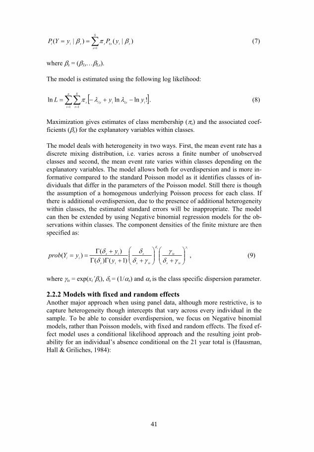
S

ssisissii yPyYP

1| )|()|( (7)

where s = ( 1s… Ls).

The model is estimated using the following log likelihood:

n

i

S

sisiisis yyL

1 1|| !lnlnln . (8)

Maximization gives estimates of class membership ( s) and the associated coef-ficients ( s) for the explanatory variables within classes.

The model deals with heterogeneity in two ways. First, the mean event rate has a discrete mixing distribution, i.e. varies across a finite number of unobserved classes and second, the mean event rate varies within classes depending on the explanatory variables. The model allows both for overdispersion and is more in-formative compared to the standard Poisson model as it identifies classes of in-dividuals that differ in the parameters of the Poisson model. Still there is though the assumption of a homogenous underlying Poisson process for each class. If there is additional overdispersion, due to the presence of additional heterogeneity within classes, the estimated standard errors will be inappropriate. The model can then be extended by using Negative binomial regression models for the ob-servations within classes. The component densities of the finite mixture are then specified as:

is y

iss

is

iss

s

is

isii y

yyYprob)1()(

)()( , (9)

where is = exp(xi’ s), s = (1/ s) and s is the class specific dispersion parameter.

2.2.2 Models with fixed and random effects Another major approach when using panel data, although more restrictive, is to capture heterogeneity though intercepts that vary across every individual in the sample. To be able to consider overdispersion, we focus on Negative binomial models, rather than Poisson models, with fixed and random effects. The fixed ef-fect model uses a conditional likelihood approach and the resulting joint prob-ability for an individual’s absence conditional on the 21 year total is (Hausman, Hall & Griliches, 1984):

41

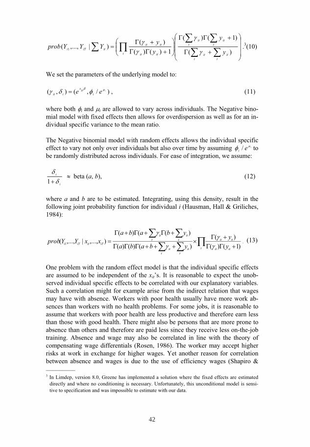
t titit

t titit

t itit

itititiTi y

y

yy

YYYprob)(

)1()(

1)()()(

)|,...,( 1 .3(10)

We set the parameters of the underlying model to:

)/,(),( iee iitx

iit , (11)

where both i and i are allowed to vary across individuals. The Negative bino-mial model with fixed effects then allows for overdispersion as well as for an in-dividual specific variance to the mean ratio.

The Negative binomial model with random effects allows the individual specific effect to vary not only over individuals but also over time by assuming iei / tobe randomly distributed across individuals. For ease of integration, we assume:

i

i

1 beta (a, b), (12)

where a and b are to be estimated. Integrating, using this density, result in the following joint probability function for individual i (Hausman, Hall & Griliches, 1984):

t itit

itit

t titit

t titit

iTitiTi yy

ybaba

ybabaxxYYprob

)1()()(

)()()(

)(()(),...,|,...,( 1 . (13)

One problem with the random effect model is that the individual specific effects are assumed to be independent of the xit’s. It is reasonable to expect the unob-served individual specific effects to be correlated with our explanatory variables. Such a correlation might for example arise from the indirect relation that wages may have with absence. Workers with poor health usually have more work ab-sences than workers with no health problems. For some jobs, it is reasonable to assume that workers with poor health are less productive and therefore earn less than those with good health. There might also be persons that are more prone to absence than others and therefore are paid less since they receive less on-the-job training. Absence and wage may also be correlated in line with the theory of compensating wage differentials (Rosen, 1986). The worker may accept higher risks at work in exchange for higher wages. Yet another reason for correlation between absence and wages is due to the use of efficiency wages (Shapiro & ––––––––– 3 In Limdep, version 8.0, Greene has implemented a solution where the fixed effects are estimated

directly and where no conditioning is necessary. Unfortunately, this unconditional model is sensi-tive to specification and was impossible to estimate with our data.

42

43

Stiglitz, 1984). By paying higher wages, employers may encourage workers to attend work. If any of these arguments apply, not controlling for unobserved het-erogeneity create a spurious relation between the wage variable, the error terms and the work absence since workers with higher wage rates, on average, have higher costs of being absent from work. The Negative binomial model with fixed effects allows for such correlation between the fixed effects and the explanatory variables.

3 Data

We use survey data from the Swedish Level of Living Survey (SLLS) combined with register data from the National Social Insurance Board (NSIB). SLLS is a survey that covers a random sample of approximately 6,000 individuals, aged be-tween 16 and 74. The surveys have been undertaken repeatedly during the last five decades and consists of interviews about the respondents’ working situation as well as personal characteristics and economic resources (See Fritzell & Lundberg, 1994, for a detailed description of the surveys). We use information from the surveys undertaken in 1974, 1981 and 1991.4

3.1 Sampling procedure

Our data has a panel structure where 6,711 individuals were interviewed in 1974, 6,985 individuals in 1981 and 6,773 in 1991. In total there are 9,079 individuals interviewed in one or several of these surveys. We focus on absence in the sense of being absent from work which is why we concentrate on people of working age (aged 20 to 64). Since one of the aspects we want to analyze is the effect of the working situation on work absence, we want to ensure that the sampled indi-viduals actually have jobs. Thus we exclude those who do not have a part-time or a full-time job at the time of the surveys. This sampling procedure leaves us with an unbalanced panel of 5,493 individuals.

3.2 Work absence measure

The absence measure used in the analysis, absence frequency, is taken from the registers at the NSIB. The absence register data includes information about all transactions made from the public sickness insurance system. As most work ab-sence are covered by public sickness insurance in Sweden, official figures are a good measure of absence and we do not have to consider the kind of bias com-mon to self-reported absence data. We have information on the annual number of absence spells during the period 1971-1991 for all the 5,493 individuals in our sample.

––––––––– 4 There is a later version of SLLS but unfortunately there is no reliable official data on absence after

1992 when the employers were made responsible for sick pay for shorter absence spells.

43

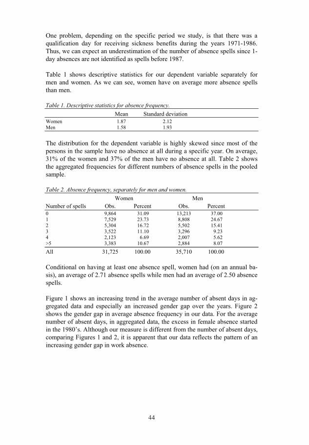
One problem, depending on the specific period we study, is that there was a qualification day for receiving sickness benefits during the years 1971-1986. Thus, we can expect an underestimation of the number of absence spells since 1-day absences are not identified as spells before 1987.

Table 1 shows descriptive statistics for our dependent variable separately for men and women. As we can see, women have on average more absence spells than men.

Table 1. Descriptive statistics for absence frequency. Mean Standard deviation Women 1.87 2.12 Men 1.58 1.93

The distribution for the dependent variable is highly skewed since most of the persons in the sample have no absence at all during a specific year. On average, 31% of the women and 37% of the men have no absence at all. Table 2 shows the aggregated frequencies for different numbers of absence spells in the pooled sample.

Table 2. Absence frequency, separately for men and women. Women Men Number of spells Obs. Percent Obs. Percent 0 9,864 31.09 13,213 37.00 1 7,529 23.73 8,808 24.67 2 5,304 16.72 5,502 15.41 3 3,522 11.10 3,296 9.23 4 2,123 6.69 2,007 5.62 >5 3,383 10.67 2,884 8.07

All 31,725 100.00 35,710 100.00

Conditional on having at least one absence spell, women had (on an annual ba-sis), an average of 2.71 absence spells while men had an average of 2.50 absence spells.

Figure 1 shows an increasing trend in the average number of absent days in ag-gregated data and especially an increased gender gap over the years. Figure 2 shows the gender gap in average absence frequency in our data. For the average number of absent days, in aggregated data, the excess in female absence started in the 1980’s. Although our measure is different from the number of absent days, comparing Figures 1 and 2, it is apparent that our data reflects the pattern of an increasing gender gap in work absence.

44

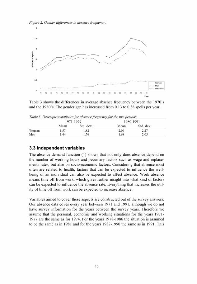
45

Figure 2. Gender differences in absence frequency.

0

0,5

1

1,5

2

2,5

3

71 72 73 74 75 76 77 78 79 80 81 82 83 84 85 86 87 88 89 90 91

Year

Nu

mb

er

of

sp

ells

Women

Men

Difference

Table 3 shows the differences in average absence frequency between the 1970’s and the 1980’s. The gender gap has increased from 0.13 to 0.38 spells per year.

Table 3. Descriptive statistics for absence frequency for the two periods.

1971-1979 1980-1991 Mean Std. dev. Mean Std. dev. Women 1.57 1.82 2.06 2.27 Men 1.44 1.76 1.68 2.05


The absence demand function (1) shows that not only does absence depend on the number of working hours and pecuniary factors such as wage and replace-ments rates, but also on socio-economic factors. Considering that absence most often are related to health, factors that can be expected to influence the well-being of an individual can also be expected to affect absence. Work absence means time off from work, which gives further insight into what kind of factors can be expected to influence the absence rate. Everything that increases the util-ity of time off from work can be expected to increase absence.

Variables aimed to cover these aspects are constructed out of the survey answers. Our absence data coves every year between 1971 and 1991, although we do not have survey information for the years between the survey years. Therefore we assume that the personal, economic and working situations for the years 1971-1977 are the same as for 1974. For the years 1978-1986 the situation is assumed to be the same as in 1981 and for the years 1987-1990 the same as in 1991. This

45

46

is a fairly strong assumption but to be able to use the rich data on annual work absence it is the only available solution.5

The variables used in the analysis are summarized in Table 4 where the descrip-tive statistics have been calculated separately for the 1970’s and the 1980’s. Sin-

gle, kids and small kids are all dummy variables. They indicate whether a person is single, has older children living at home or has small children (< 6 years old) living at home. The pressure of family responsibility is of course even greater if the individual is a lone parent, which is why in our models we will include inter-actions of the variables single and kids.

We include the education variables high school and university in our analysis in-dicating whether the highest level of education is a high school degree or a uni-versity degree. The standard human capital variable “education” is suggested as an appropriate measure and empirically found by Grossman (1972) to increase health productivity.

Wage is measured as the hourly wage rate, deflated by the Consumer Price Index with 1980 as the base year. The reform dummies, ref74, ref87 and ref91, are in-cluded in the analysis to reflect changes in the sickness insurance system and thus changes in the cost of absence. Before 1974 there was a qualification day for which no benefit was paid. Between 1974 and 1987 this qualification day could be avoided by reporting sick (to an answering machine) before midnight the preceding day. In 1987 the qualification was abolished and all sick spells were covered no matter how short. In addition, before 1974 the compensation was untaxed and could vary depending on what day of the week it was or on the insured person’s family characteristics. Our reform dummy (ref74) indicates that the overall level of compensation from the sickness benefit system was substan-tially raised in 1974. The level was then made uniform and raised to 90 % for everybody in 1987. Note that the dummy for the reform of 1987 also indicates that the official statistics of work absence from 1987 and onward include the first day of a sickness spell; the statistics did not always show this before the reform. The reform in 1991, on the other hand, increased the cost of absence, especially for absences of shorter duration as the replacement rate was cut.

Due to measurement problems we have no variable measuring virtual income. However, previous studies have also reported problems with measuring income and received relatively low precision in their estimates (Johansson & Palme, 2002).

Part-time is a dummy variable included as a proxy for contracted working hours and shift indicates whether a person works shift or not. Shorter is a dummy vari-

––––––––– 5 All of our estimations have been done on data only covering the three survey years as well. The

main results remain essentially the same although there are slightly fewer significant parameter es-timates.

46

47

able indicating if the person desires fewer working hours and serve as an indica-tor for the use of absence as a measure for reaching the optimal work–leisure combination (Dunn & Youngblood, 1986).

One important element of the socio-economic variables is of course health status. The SLLS surveys contain several questions concerning health. We use 14 of these for which a physician has most likely made a diagnosis, and which are primarily not affected by poor working conditions. We are interested in control-ling for differences in health status rather than analyzing the impact of specific health deficiencies, which is why we then further reduce the health variables by a principal component (PC) analysis (see Appendix). In the following analysis the five first PC’s, H1-H5, are included, accounting for nearly 50 percent of the variation in the health related variables.

The SLLS surveys also include several questions concerning working environ-ment. Many of these variables have the same expected influence on work ab-sence and are highly correlated, therefore we reduce them by performing another PC analysis (see Appendix). From the 12 working environment variables we ex-tracted four PC’s, W1-W4, covering about 55 percent of the variation in these variables.6

Since absence imposes costs and uncertainty on employers, it might serve the employer to check on the employees through different kinds of monitoring de-vices. We have included two variables, imptime (important to be on time) and punch (the use of a time-clock at the work place), to measure the level of moni-toring (following Johansson & Palme, 1996; 2002 and Johansson & Brännäs, 1998).

Unemployment, ue, measured as the annual average unemployment rate for each year is included in the analysis since absence can be expected to be correlated with the level of unemployment (Leigh, 1985; Arai & Skogman Thoursie, 2004).

––––––––– 6 Estimations have been made using all the original health and working conditions variables as well,

but the results remain essentially unchanged.

47

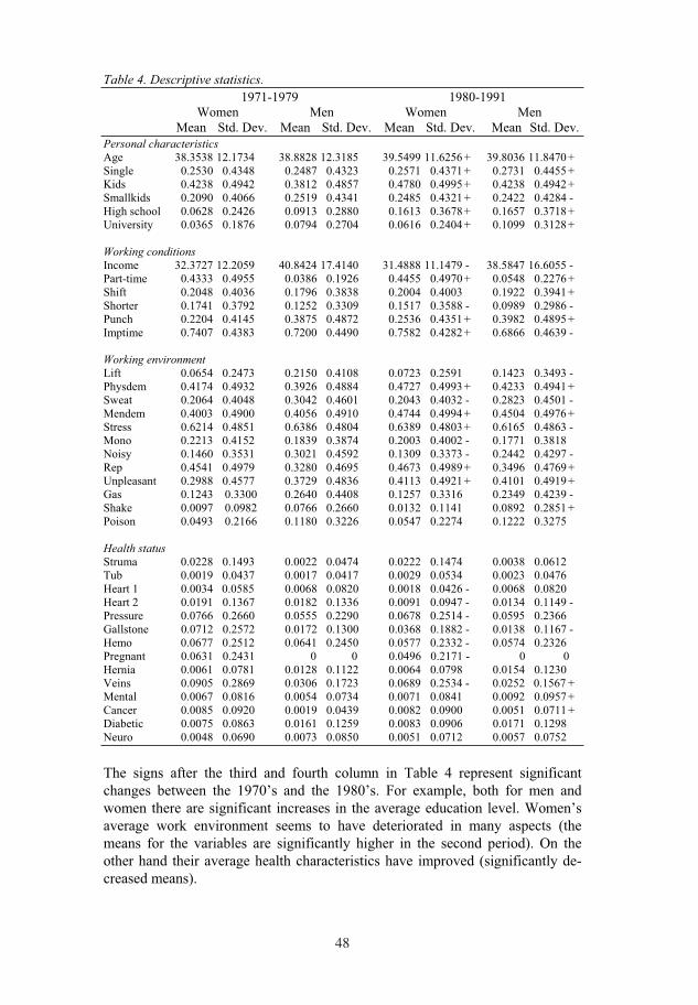
48

Table 4. Descriptive statistics.

1971-1979 1980-1991 Women Men Women Men Mean Std. Dev. Mean Std. Dev. Mean Std. Dev. Mean Std. Dev. Personal characteristics

Age 38.3538 12.1734 38.8828 12.3185 39.5499 11.6256 + 39.8036 11.8470 + Single 0.2530 0.4348 0.2487 0.4323 0.2571 0.4371 + 0.2731 0.4455 + Kids 0.4238 0.4942 0.3812 0.4857 0.4780 0.4995 + 0.4238 0.4942 + Smallkids 0.2090 0.4066 0.2519 0.4341 0.2485 0.4321 + 0.2422 0.4284 - High school 0.0628 0.2426 0.0913 0.2880 0.1613 0.3678 + 0.1657 0.3718 + University 0.0365 0.1876 0.0794 0.2704 0.0616 0.2404 + 0.1099 0.3128 +

Working conditions

Income 32.3727 12.2059 40.8424 17.4140 31.4888 11.1479 - 38.5847 16.6055 - Part-time 0.4333 0.4955 0.0386 0.1926 0.4455 0.4970 + 0.0548 0.2276 + Shift 0.2048 0.4036 0.1796 0.3838 0.2004 0.4003 0.1922 0.3941 + Shorter 0.1741 0.3792 0.1252 0.3309 0.1517 0.3588 - 0.0989 0.2986 - Punch 0.2204 0.4145 0.3875 0.4872 0.2536 0.4351 + 0.3982 0.4895 + Imptime 0.7407 0.4383 0.7200 0.4490 0.7582 0.4282 + 0.6866 0.4639 -

Working environment

Lift 0.0654 0.2473 0.2150 0.4108 0.0723 0.2591 0.1423 0.3493 - Physdem 0.4174 0.4932 0.3926 0.4884 0.4727 0.4993 + 0.4233 0.4941 + Sweat 0.2064 0.4048 0.3042 0.4601 0.2043 0.4032 - 0.2823 0.4501 - Mendem 0.4003 0.4900 0.4056 0.4910 0.4744 0.4994 + 0.4504 0.4976 + Stress 0.6214 0.4851 0.6386 0.4804 0.6389 0.4803 + 0.6165 0.4863 - Mono 0.2213 0.4152 0.1839 0.3874 0.2003 0.4002 - 0.1771 0.3818 Noisy 0.1460 0.3531 0.3021 0.4592 0.1309 0.3373 - 0.2442 0.4297 - Rep 0.4541 0.4979 0.3280 0.4695 0.4673 0.4989 + 0.3496 0.4769 + Unpleasant 0.2988 0.4577 0.3729 0.4836 0.4113 0.4921 + 0.4101 0.4919 + Gas 0.1243 0.3300 0.2640 0.4408 0.1257 0.3316 0.2349 0.4239 - Shake 0.0097 0.0982 0.0766 0.2660 0.0132 0.1141 0.0892 0.2851 + Poison 0.0493 0.2166 0.1180 0.3226 0.0547 0.2274 0.1222 0.3275

Health status

Struma 0.0228 0.1493 0.0022 0.0474 0.0222 0.1474 0.0038 0.0612 Tub 0.0019 0.0437 0.0017 0.0417 0.0029 0.0534 0.0023 0.0476 Heart 1 0.0034 0.0585 0.0068 0.0820 0.0018 0.0426 - 0.0068 0.0820 Heart 2 0.0191 0.1367 0.0182 0.1336 0.0091 0.0947 - 0.0134 0.1149 - Pressure 0.0766 0.2660 0.0555 0.2290 0.0678 0.2514 - 0.0595 0.2366 Gallstone 0.0712 0.2572 0.0172 0.1300 0.0368 0.1882 - 0.0138 0.1167 - Hemo 0.0677 0.2512 0.0641 0.2450 0.0577 0.2332 - 0.0574 0.2326 Pregnant 0.0631 0.2431 0 0 0.0496 0.2171 - 0 0 Hernia 0.0061 0.0781 0.0128 0.1122 0.0064 0.0798 0.0154 0.1230 Veins 0.0905 0.2869 0.0306 0.1723 0.0689 0.2534 - 0.0252 0.1567 + Mental 0.0067 0.0816 0.0054 0.0734 0.0071 0.0841 0.0092 0.0957 + Cancer 0.0085 0.0920 0.0019 0.0439 0.0082 0.0900 0.0051 0.0711 + Diabetic 0.0075 0.0863 0.0161 0.1259 0.0083 0.0906 0.0171 0.1298 Neuro 0.0048 0.0690 0.0073 0.0850 0.0051 0.0712 0.0057 0.0752

The signs after the third and fourth column in Table 4 represent significant changes between the 1970’s and the 1980’s. For example, both for men and women there are significant increases in the average education level. Women’s average work environment seems to have deteriorated in many aspects (the means for the variables are significantly higher in the second period). On the other hand their average health characteristics have improved (significantly de-creased means).

48

49

4 Results

The empirical analysis is divided into two parts. We first concentrate on the gen-der differences in absence levels by analyzing the gender gap during the 1980’s. We then continue by analyzing the increased gender gap over time using the en-tire period covered by the data, 1971-1991.

4.1 Gender differences in absence levels

4.1.1 Model selection We start the model selection process by estimating the standard model for count data, i.e. the Poisson model. As Table 5 shows, we find clear evidence of overdispersion for both the male and the female sub sample.

Table 5. Test of overdispersion in absence frequency. Estimation results, for women and

men, from the regression tests suggested by Cameron & Trivedi (1990).7

g( i ) = i g( i ) = i2

Coefficient t-ratio p-value Coefficient t-ratio p-value

Women 1.1480 34.13 0.0000 0.5394 35.10 0.0000

Men 1.2101 33.56 0.0000 0.6594 33.20 0.0000

One reasonable explanation to overdispersion is the presence of unobserved het-erogeneity. We thus estimate models accommodating for this heterogeneity. Ta-ble 6 presents the likelihood values for the different models. The lower panel shows test statistics used for the model selection. To test the independence as-sumption of the Negative binomial model with random effects, a Hausman test is performed between the fixed effects and the random effects model. As Table 6 shows, the hypothesis of independence can be rejected.

In estimating the finite mixture models the likelihood functions have problems of convergence for certain numbers of latent classes and the Hessian matrix cannot be inverted to get the standard errors. A plausible explanation is that there is too much collinearity among the columns (corresponding to estimated parameters) of the Hessian matrix. This implies that at least some of the estimated parameters are highly correlated and that one point of support is not sufficiently different from the others for the inverse to be computationally feasible (D’Unger & Land, 1998). Even if the models are re-estimated with simpler specifications this prob-lems remain. Additionally the finite mixture models based on Negative binomial

––––––––– 7 The hypothesis to be tested is: H0: Var[yi] = E[yi] versus H1: Var[yi] = E[yi] + g(E[yi]). The test is


iiiiiyyz on )2/()(

iigw , where i is the pre-

dicted value from the Poisson regression. Cameron & Trivedi suggest two possibilities for g( i);g( i ) = i or g( i ) = i

2 . A simple t-test of whether the coefficient in the regression of z on w, when g( i ) is specified in either way, is significantly different from zero tests H0 versus H1.

49

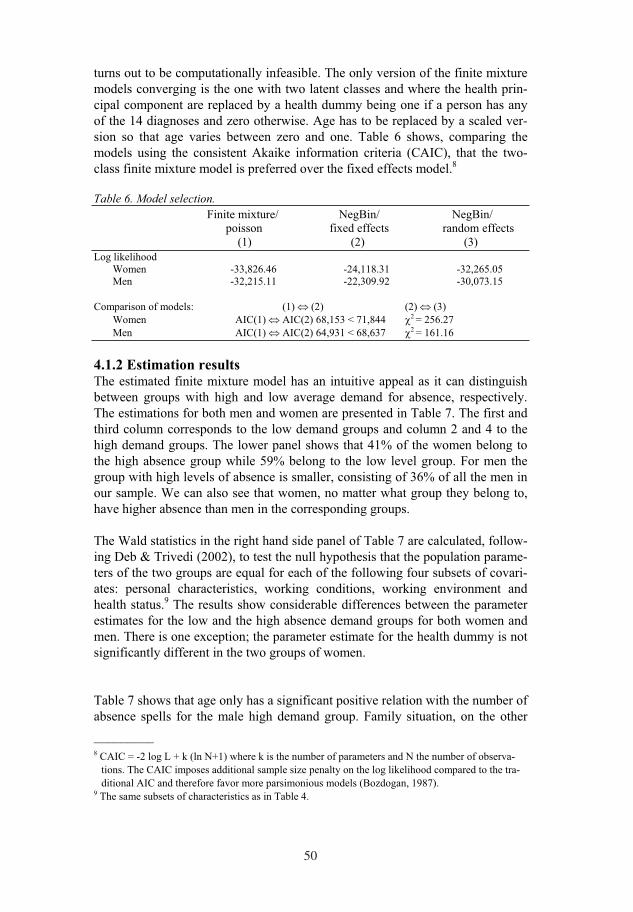
50

turns out to be computationally infeasible. The only version of the finite mixture models converging is the one with two latent classes and where the health prin-cipal component are replaced by a health dummy being one if a person has any of the 14 diagnoses and zero otherwise. Age has to be replaced by a scaled ver-sion so that age varies between zero and one. Table 6 shows, comparing the models using the consistent Akaike information criteria (CAIC), that the two-class finite mixture model is preferred over the fixed effects model.8

Table 6. Model selection.

Finite mixture/ NegBin/ NegBin/ poisson fixed effects random effects (1) (2) (3) Log likelihood Women -33,826.46 -24,118.31 -32,265.05 Men -32,215.11 -22,309.92 -30,073.15

Comparison of models: (1) (2) (2) (3) Women AIC(1) AIC(2) 68,153 < 71,844 2 = 256.27 Men AIC(1) AIC(2) 64,931 < 68,637 2 = 161.16

4.1.2 Estimation results The estimated finite mixture model has an intuitive appeal as it can distinguish between groups with high and low average demand for absence, respectively. The estimations for both men and women are presented in Table 7. The first and third column corresponds to the low demand groups and column 2 and 4 to the high demand groups. The lower panel shows that 41% of the women belong to the high absence group while 59% belong to the low level group. For men the group with high levels of absence is smaller, consisting of 36% of all the men in our sample. We can also see that women, no matter what group they belong to, have higher absence than men in the corresponding groups.

The Wald statistics in the right hand side panel of Table 7 are calculated, follow-ing Deb & Trivedi (2002), to test the null hypothesis that the population parame-ters of the two groups are equal for each of the following four subsets of covari-ates: personal characteristics, working conditions, working environment and health status.9 The results show considerable differences between the parameter estimates for the low and the high absence demand groups for both women and men. There is one exception; the parameter estimate for the health dummy is not significantly different in the two groups of women.

Table 7 shows that age only has a significant positive relation with the number of absence spells for the male high demand group. Family situation, on the other

––––––––– 8 CAIC = -2 log L + k (ln N+1) where k is the number of parameters and N the number of observa-

tions. The CAIC imposes additional sample size penalty on the log likelihood compared to the tra-ditional AIC and therefore favor more parsimonious models (Bozdogan, 1987).

9 The same subsets of characteristics as in Table 4.

50

51

hand, tends to have different effect in the separate groups. It is only in the high absence demand group of women that both small children and older children de-crease absence frequency. Women belonging to the low demand group act more like men for which small children increases the number of absence spells while older children decrease absence frequency. Being a single results in higher ab-sence for those men and women who belong to the high level groups, while both male and female singles in the low level groups have less absence compared to people who live together with someone. Men, no matter which group they be-long to, have less absence if they have a mentally demanding work, while female absence increases the more mentally demanding work they have. The reform in 1987, which raised the generosity in the sickness insurance system, increased ab-sence frequency for all groups except the male low demand group. On the other hand, it was only the high demand groups, men as well as women, who de-creased the number of absence spells when the replacement rates were cut in 1991.

As Table 8 shows, also the observed characteristics differ between the low and the high absence demand groups. Men and women in the groups with high aver-age demand have worse work environment and poorer health than the other groups. We can also see that women with low average absence are older, have fewer children, are married to a greater extent, have higher education and are less often lone parents than the women with high absence. Concerning children the pattern is the reversed for men. Men with low absence are those who have more children and more often are lone parents.

51

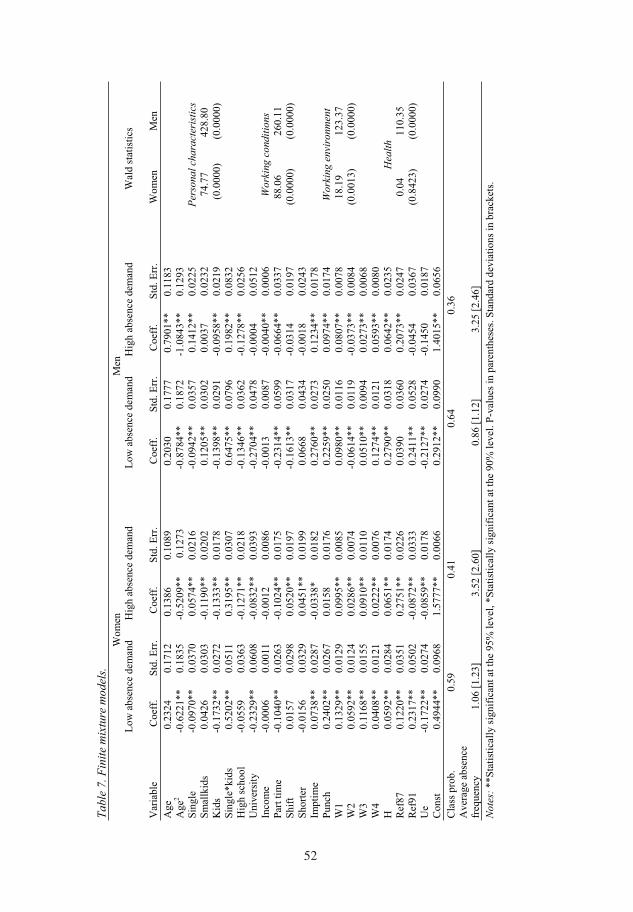
Table

7.

Fin

ite

mix

ture

model

s.

W

omen

M

en

Low

abs

ence

dem

and

H

igh

abse

nce

dem

and

Low

abs

ence

dem

and

H

igh

abse

nce

dem

and

Wal

d st

atis

tics

Var

iabl

e

Coe

ff.

S

td. E

rr.

Coe

ff.

Std

. Err

. C

oeff

. S

td. E

rr.

Coe

ff.

Std

. Err

. W

omen

Men

Age

0.23

24

0.

1712

0.13

86

0.10

89

0

.203

0

0.1

777

0

.790

1**

0.11

83

A

ge2

-

0.62

21**

0.18

35

-0.5

209*

*

0.

1273

-0.8

784*

*

0.

1872

-

1.08

43**

0.12

93

S

ingl

e -0

.097

0**

0.

0370

0

.057

4**

0.

0216

-0.

0942

**

0.03

57

0.1

412*

*

0.02

25

Per

sonal

chara

cter

isti

cs

Sm

allk

ids

0.0

426

0.

0303

-0

.119

0**

0.

0202

0.1

205*

* 0.

0302

0

.003

7

0.02

32

74.

77

428.

80

Kid

s

-0.1

732*

* 0.

0272

-0

.133

3**

0.

0178

-

0.13

98**

0.

0291

-0

.095

8**

0

.021

9

(0.0

000)

(0.0

000)

S

ingl

e*ki

ds

0.52

02**

0.

0511

0

.319

5**

0.

0307

0

.647

5**

0.07

96

0.

1982

**

0.08

32

H

igh

scho

ol

-0.0

559

0.

0363

-0

.127

1**

0.

0218

-0.1

346*

* 0.

0362

-0

.127

8**

0.

0256

Uni

vers

ity

-0.2

329*

* 0.

0608

-

0.08

32**

0.

0393

-

0.27

04**

0.

0478

-0

.000

4

0.05

12

Inco

me

-0.0

006

0.

0011

-

0.00

12

0.00

86

-0.

0013

0.

0087

-0

.004

0**

0

.000

6

Wo

rkin

gco

ndit

ions

Par

t ti

me

-

0.10

40**

0.

0263

-0

.102

4**

0.

0175

-0

.231

4**

0.05

99

-0.

0664

**

0.03

37

88

.06

26

0.11

S

hift

0.

0157

0.

0298

0

.052

0**

0.

0197

-

0.16

13**

0.

0317

-0

.031

4

0.01

97

(0.0

000)

(0

.000

0)

Sho

rter

-0

.015

6

0.03

29

0.0

451*

*

0.01

99

0.0

668

0.

0434

-0

.001

8

0.0

243

Impt

ime

0.07

38**

0.

0287

-0

.033

8*

0.01

82

0

.276

0**

0.02

73

0.1

234*

*

0.01

78

Pun

ch

0.

2402

**

0.02

67

0.0

158

0.

0176

0.

2259

**

0.02

50

0.09

74**

0.

0174

W

ork

ing

en

viro

nm

ent

W1

0.

1329

**

0.01

29

0.0

995*

*

0.00

85

0.09

80**

0.

0116

0

.080

7**

0.

0078

18.1

9 12

3.37

W

2 0

.059

2**

0.

0124

0.

0286

**

0.00

74

-0.

0614

**

0.01

19

-0.

0373

**

0.00

84

(0.0

013)

(0

.000

0)

W3

0.1

168*

*

0.01

55

0.0

910*

*

0.01

10

0.05

10**

0

.009

4

0.0

273*

*

0.00

68

W4

0.04

08**

0.

0121

0

.022

2**

0.

0076

0.

1274

**

0.01

21

0.0

593*

*

0.00

80

H

0.05

92**

0.

0284

0.

0651

**

0.01

74

0.27

90**

0.

0318

0

.064

2**

0.

0235

Hea

lth

Ref

87

0

.122

0**

0.

0351

0

.275

1**

0.

0226

0.03

90

0.03

60

0.2

073*

*

0.0

247

0.

04

11

0.35

R

ef91

0

.231

7**

0.

0502

-0

.087

2**

0.

0333

0

.241

1**

0.05

28

-0.0

454

0.

0367

(0

.842

3)

(0

.000

0)

Ue

-0.

1722

**

0.02

74

-0.0

859*

*

0.01

78

-0.2

127*

* 0.

0274

-

0.14

50

0.01

87

C

onst

0.49

44**

0.

0968

1.

5777

**

0.00

66

0.

2912

**

0.09

90

1.4

015*

* 0.

0656

Cla

ss p

rob.

0.

59

0.41

0.

64

0.36

A

vera

ge a

bsen

ce

freq

uenc

y 1.

06 [

1.23

] 3.

52 [

2.60

] 0.

86 [

1.12

] 3.

25 [

2.46

]

Note

s: *

*Sta

tist

ical

ly s

igni

fica

nt a

t the

95%

leve

l, *

Sta

tist

ical

ly s

igni

fica

nt a

t the

90%

leve

l. P

-val

ues

in p

aren

thes

es. S

tand

ard

devi

atio

ns in

bra

cket

s.

52

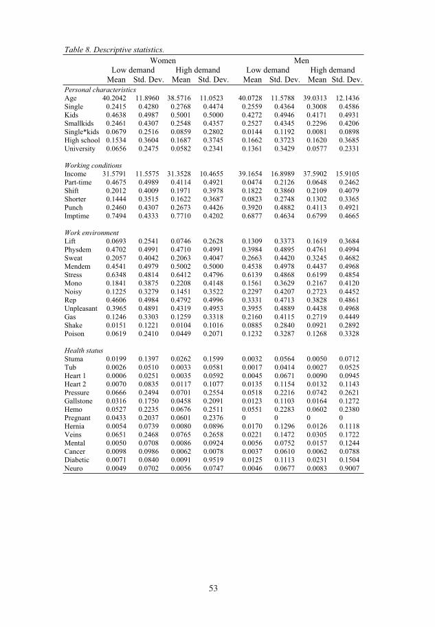
5353

Table 8. Descriptive statistics.

Women Men Low demand High demand Low demand High demand Mean Std. Dev. Mean Std. Dev. Mean Std. Dev. Mean Std. Dev. Personal characteristics

Age 40.2042 11.8960 38.5716 11.0523 40.0728 11.5788 39.0313 12.1436 Single 0.2415 0.4280 0.2768 0.4474 0.2559 0.4364 0.3008 0.4586 Kids 0.4638 0.4987 0.5001 0.5000 0.4272 0.4946 0.4171 0.4931 Smallkids 0.2461 0.4307 0.2548 0.4357 0.2527 0.4345 0.2296 0.4206 Single*kids 0.0679 0.2516 0.0859 0.2802 0.0144 0.1192 0.0081 0.0898 High school 0.1534 0.3604 0.1687 0.3745 0.1662 0.3723 0.1620 0.3685 University 0.0656 0.2475 0.0582 0.2341 0.1361 0.3429 0.0577 0.2331

Working conditions

Income 31.5791 11.5575 31.3528 10.4655 39.1654 16.8989 37.5902 15.9105 Part-time 0.4675 0.4989 0.4114 0.4921 0.0474 0.2126 0.0648 0.2462 Shift 0.2012 0.4009 0.1971 0.3978 0.1822 0.3860 0.2109 0.4079 Shorter 0.1444 0.3515 0.1622 0.3687 0.0823 0.2748 0.1302 0.3365 Punch 0.2460 0.4307 0.2673 0.4426 0.3920 0.4882 0.4113 0.4921 Imptime 0.7494 0.4333 0.7710 0.4202 0.6877 0.4634 0.6799 0.4665

Work environment

Lift 0.0693 0.2541 0.0746 0.2628 0.1309 0.3373 0.1619 0.3684 Physdem 0.4702 0.4991 0.4710 0.4991 0.3984 0.4895 0.4761 0.4994 Sweat 0.2057 0.4042 0.2063 0.4047 0.2663 0.4420 0.3245 0.4682 Mendem 0.4541 0.4979 0.5002 0.5000 0.4538 0.4978 0.4437 0.4968 Stress 0.6348 0.4814 0.6412 0.4796 0.6139 0.4868 0.6199 0.4854 Mono 0.1841 0.3875 0.2208 0.4148 0.1561 0.3629 0.2167 0.4120 Noisy 0.1225 0.3279 0.1451 0.3522 0.2297 0.4207 0.2723 0.4452 Rep 0.4606 0.4984 0.4792 0.4996 0.3331 0.4713 0.3828 0.4861 Unpleasant 0.3965 0.4891 0.4319 0.4953 0.3955 0.4889 0.4438 0.4968 Gas 0.1246 0.3303 0.1259 0.3318 0.2160 0.4115 0.2719 0.4449 Shake 0.0151 0.1221 0.0104 0.1016 0.0885 0.2840 0.0921 0.2892 Poison 0.0619 0.2410 0.0449 0.2071 0.1232 0.3287 0.1268 0.3328

Health status

Stuma 0.0199 0.1397 0.0262 0.1599 0.0032 0.0564 0.0050 0.0712 Tub 0.0026 0.0510 0.0033 0.0581 0.0017 0.0414 0.0027 0.0525 Heart 1 0.0006 0.0251 0.0035 0.0592 0.0045 0.0671 0.0090 0.0945 Heart 2 0.0070 0.0835 0.0117 0.1077 0.0135 0.1154 0.0132 0.1143 Pressure 0.0666 0.2494 0.0701 0.2554 0.0518 0.2216 0.0742 0.2621 Gallstone 0.0316 0.1750 0.0458 0.2091 0.0123 0.1103 0.0164 0.1272 Hemo 0.0527 0.2235 0.0676 0.2511 0.0551 0.2283 0.0602 0.2380 Pregnant 0.0433 0.2037 0.0601 0.2376 0 0 0 0 Hernia 0.0054 0.0739 0.0080 0.0896 0.0170 0.1296 0.0126 0.1118 Veins 0.0651 0.2468 0.0765 0.2658 0.0221 0.1472 0.0305 0.1722 Mental 0.0050 0.0708 0.0086 0.0924 0.0056 0.0752 0.0157 0.1244 Cancer 0.0098 0.0986 0.0062 0.0078 0.0037 0.0610 0.0062 0.0788 Diabetic 0.0071 0.0840 0.0091 0.9519 0.0125 0.1113 0.0231 0.1504 Neuro 0.0049 0.0702 0.0056 0.0747 0.0046 0.0677 0.0083 0.9007

53

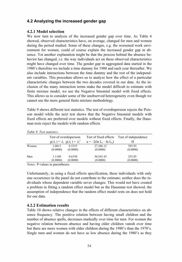
5454

4.2 Analyzing the increased gender gap

4.2.1 Model selection We now turn to analysis of the increased gender gap over time. As Table 4 showed, observed characteristics have, on average, changed for men and women during the period studied. Some of these changes, e.g. the worsened work envi-ronment for women, could of course explain the increased gender gap in ab-sence. Yet another explanation might be that the process behind the absence be-havior has changed, i.e. the way individuals act on these observed characteristics might have changed over time. The gender gap in aggregated data started in the 1980’s therefore we include a time dummy for 1980 and each year thereafter. We also include interactions between the time dummy and the rest of the independ-ent variables. This procedure allows us to analyze how the effect of a particular characteristic changes between the two decades covered in our data. As the in-clusion of the many interaction terms make the model difficult to estimate with finite mixture model, we use the Negative binomial model with fixed effects. This allows us to consider some of the unobserved heterogeneity even though we cannot use the more general finite mixture methodology.

Table 9 shows different test statistics. The test of overdispersion rejects the Pois-son model while the next test shows that the Negative binomial models with fixed effects are preferred over models without fixed effects. Finally, the Haus-man tests reject the models with random effects.

Table 9. Test statistics.

Test of overdispersion Test of fixed effects Test of independence

g( i ) = i g( i ) = i2 a = –2(ln Lr – ln Lu) H

Women 1.0813 0.5355 27,386.12 395.93 (0.0000) (0.0000) (0.0000) (0.0000)

Men 1.1109 0.6350 30,543.43 255.05 (0.0000) (0.0000) (0.0000) (0.0000)

Notes: P-values in parentheses.

Unfortunately, in using a fixed effects specification, these individuals with only one occurrence in the panel do not contribute to the estimate; neither does the in-dividuals whose dependent variable never changes. This would not have created a problem in fitting a random effect model but as the Hausman test showed, the assumption of independence that the random effect model rests on does not hold for our data.

4.2.2 Estimation results Table 10 shows relative changes in the effects of different characteristics on ab-sence frequency. The positive relation between having small children and the number of absence spells, decreases markedly over time for men. For women the negative relation between absence and having older children vanish over time but there are more women with older children during the 1980’s than the 1970’s. Single men and women do not have as low absence during the 1980’s as they

54

5555

had earlier. The effect is stronger for women who also are single to a greater ex-tent during the second period. Lone parent women do not have as much higher absence during the later period as they did earlier. It might be that living as a single parent is easier during the 1980’s due to for example the improved child care arrangements. The strong negative relation between working part time and absence loses up during the second period. At the same time there are a greater share of the women that works part time over the years. Unemployment does not decrease female absence frequency as much as it did during first period. The ef-fects of working environment also change over time; some affect absence more and some less. Physically demanding work increases female absence more than before while mentally demanding work is managed more successfully. Repeti-tive and monotonous types of work seem to have a smaller effect on women’s absence in the second period while men are less affected by hazardous work en-vironment.

55

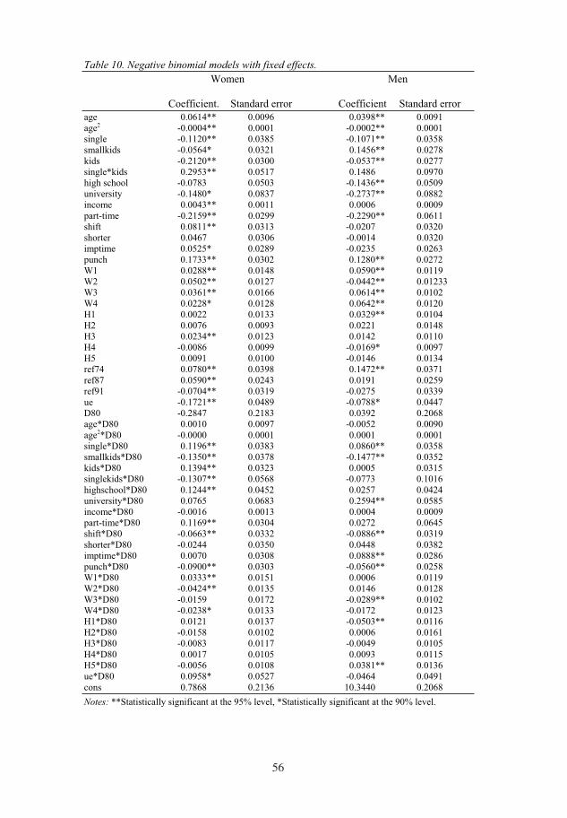
5656

Table 10. Negative binomial models with fixed effects.

Women Men

Coefficient. Standard error Coefficient Standard error age 0.0614** 0.0096 0.0398** 0.0091 age2 -0.0004** 0.0001 -0.0002** 0.0001 single -0.1120** 0.0385 -0.1071** 0.0358 smallkids -0.0564* 0.0321 0.1456** 0.0278 kids -0.2120** 0.0300 -0.0537** 0.0277 single*kids 0.2953** 0.0517 0.1486 0.0970 high school -0.0783 0.0503 -0.1436** 0.0509 university -0.1480* 0.0837 -0.2737** 0.0882 income 0.0043** 0.0011 0.0006 0.0009 part-time -0.2159** 0.0299 -0.2290** 0.0611 shift 0.0811** 0.0313 -0.0207 0.0320 shorter 0.0467 0.0306 -0.0014 0.0320 imptime 0.0525* 0.0289 -0.0235 0.0263 punch 0.1733** 0.0302 0.1280** 0.0272 W1 0.0288** 0.0148 0.0590** 0.0119 W2 0.0502** 0.0127 -0.0442** 0.01233 W3 0.0361** 0.0166 0.0614** 0.0102 W4 0.0228* 0.0128 0.0642** 0.0120 H1 0.0022 0.0133 0.0329** 0.0104 H2 0.0076 0.0093 0.0221 0.0148 H3 0.0234** 0.0123 0.0142 0.0110 H4 -0.0086 0.0099 -0.0169* 0.0097 H5 0.0091 0.0100 -0.0146 0.0134 ref74 0.0780** 0.0398 0.1472** 0.0371 ref87 0.0590** 0.0243 0.0191 0.0259 ref91 -0.0704** 0.0319 -0.0275 0.0339 ue -0.1721** 0.0489 -0.0788* 0.0447 D80 -0.2847 0.2183 0.0392 0.2068 age*D80 0.0010 0.0097 -0.0052 0.0090 age2*D80 -0.0000 0.0001 0.0001 0.0001 single*D80 0.1196** 0.0383 0.0860** 0.0358 smallkids*D80 -0.1350** 0.0378 -0.1477** 0.0352 kids*D80 0.1394** 0.0323 0.0005 0.0315 singlekids*D80 -0.1307** 0.0568 -0.0773 0.1016 highschool*D80 0.1244** 0.0452 0.0257 0.0424 university*D80 0.0765 0.0683 0.2594** 0.0585 income*D80 -0.0016 0.0013 0.0004 0.0009 part-time*D80 0.1169** 0.0304 0.0272 0.0645 shift*D80 -0.0663** 0.0332 -0.0886** 0.0319 shorter*D80 -0.0244 0.0350 0.0448 0.0382 imptime*D80 0.0070 0.0308 0.0888** 0.0286 punch*D80 -0.0900** 0.0303 -0.0560** 0.0258 W1*D80 0.0333** 0.0151 0.0006 0.0119 W2*D80 -0.0424** 0.0135 0.0146 0.0128 W3*D80 -0.0159 0.0172 -0.0289** 0.0102 W4*D80 -0.0238* 0.0133 -0.0172 0.0123 H1*D80 0.0121 0.0137 -0.0503** 0.0116 H2*D80 -0.0158 0.0102 0.0006 0.0161 H3*D80 -0.0083 0.0117 -0.0049 0.0105 H4*D80 0.0017 0.0105 0.0093 0.0115 H5*D80 -0.0056 0.0108 0.0381** 0.0136 ue*D80 0.0958* 0.0527 -0.0464 0.0491 cons 0.7868 0.2136 10.3440 0.2068

Notes: **Statistically significant at the 95% level, *Statistically significant at the 90% level.

56

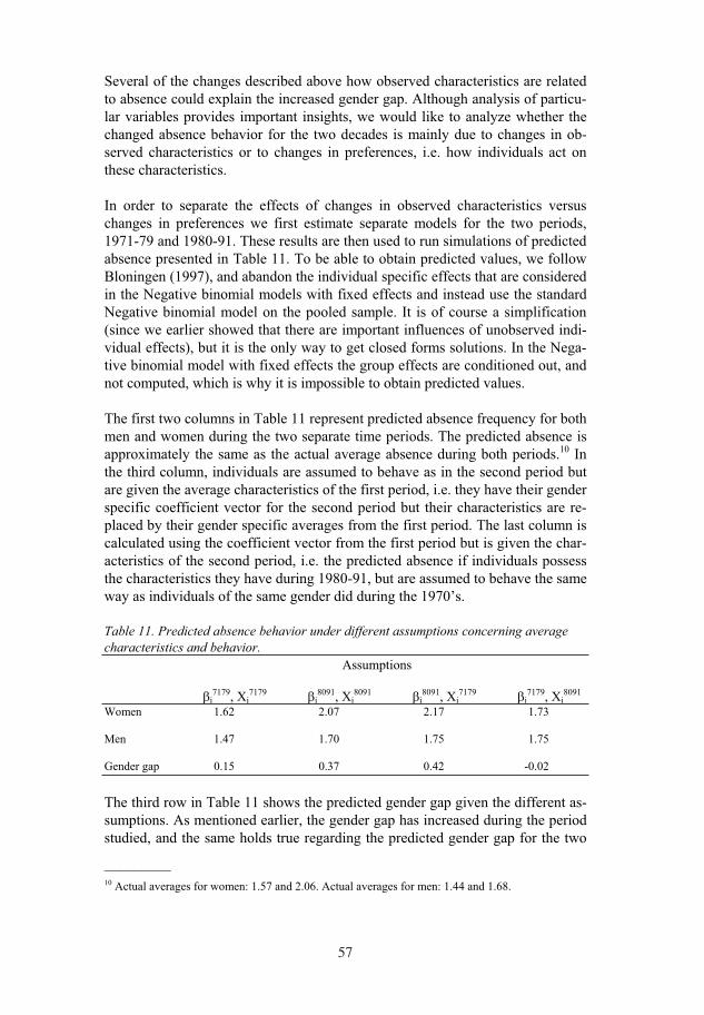
5757

Several of the changes described above how observed characteristics are related to absence could explain the increased gender gap. Although analysis of particu-lar variables provides important insights, we would like to analyze whether the changed absence behavior for the two decades is mainly due to changes in ob-served characteristics or to changes in preferences, i.e. how individuals act on these characteristics.

In order to separate the effects of changes in observed characteristics versus changes in preferences we first estimate separate models for the two periods, 1971-79 and 1980-91. These results are then used to run simulations of predicted absence presented in Table 11. To be able to obtain predicted values, we follow Bloningen (1997), and abandon the individual specific effects that are considered in the Negative binomial models with fixed effects and instead use the standard Negative binomial model on the pooled sample. It is of course a simplification (since we earlier showed that there are important influences of unobserved indi-vidual effects), but it is the only way to get closed forms solutions. In the Nega-tive binomial model with fixed effects the group effects are conditioned out, and not computed, which is why it is impossible to obtain predicted values.

The first two columns in Table 11 represent predicted absence frequency for both men and women during the two separate time periods. The predicted absence is approximately the same as the actual average absence during both periods.10 In the third column, individuals are assumed to behave as in the second period but are given the average characteristics of the first period, i.e. they have their gender specific coefficient vector for the second period but their characteristics are re-placed by their gender specific averages from the first period. The last column is calculated using the coefficient vector from the first period but is given the char-acteristics of the second period, i.e. the predicted absence if individuals possess the characteristics they have during 1980-91, but are assumed to behave the same way as individuals of the same gender did during the 1970’s.

Table 11. Predicted absence behavior under different assumptions concerning average

characteristics and behavior.

Assumptions

i7179, Xi

7179 i8091, Xi

8091i8091, Xi

7179i7179, Xi

8091

Women 1.62 2.07 2.17 1.73

Men 1.47 1.70 1.75 1.75

Gender gap 0.15 0.37 0.42 -0.02

The third row in Table 11 shows the predicted gender gap given the different as-sumptions. As mentioned earlier, the gender gap has increased during the period studied, and the same holds true regarding the predicted gender gap for the two

––––––––– 10 Actual averages for women: 1.57 and 2.06. Actual averages for men: 1.44 and 1.68.

57

5858

time periods (0.37 compared to 0.15). According to the third column, the gender gap would have been even greater if the average characteristics had remained the same during the 1980’s as they had been during the 1970’s. The fourth column, on the other hand, shows that there would have been no gender gap if the behav-iors of men and women had remained the same during both periods studied. An interesting result is that men seem to have adjusted their absence behavior to their observed characteristics during the 1980’s, as their predicted absence in the second column actually is lower than the predicted absence under the assump-tions in the third and fourth columns. The main conclusion from Table 11 is that the increased gender gap in work absence can be attributed to changes in how women act on observed characteristics rather than changes in observable charac-teristics. Another contribution to the increased gender gap is the fact that men, given their changed observed characteristics, have adjusted their absence behav-ior and have decreased their absence.

5 Conclusions

Using panel data covering 21 years and almost 5,500 individuals, we have found interesting gender differences in absence. Women have higher absence levels than men for the entire period, but the gender gap have increased during the years studied.

In our analysis of gender differences in absence levels, we find that men and women act differently on the observed characteristics. In addition to these find-ings, our analysis reveals that there are groups within each gender that have sepa-rate absence behaviors. Our use of finite mixture models show that both men and women can be divided into groups with high and low average demand of ab-sence. The absence behavior differs as much between the separate groups within gender as it does between men and women.

About 41% of the women in our sample belong to the high absence demand group which is a group with women having more children, lower education, liv-ing alone in a greater extent, are lone parent more often, work more full time and also have worse work environment and poorer health than the other women. Some of these characteristics in known to increase absence, but taken together they also represent a heavy double burden on these women. This burden may, in line with Paringer (1983), lead to use of absence as an investment in health. We know that women on average recognize and treat health problems at an earlier stage than men. Thus, women in the high demand group may also use repeated absence spells to a greater extent than men or women in the low demand group to take care of themselves.

Our analysis of the increased gender gap over time shows that not only have there been changes in the average observed characteristics, but there have also been changes in the way individuals act on these characteristics. The increased gender gap over time can actually be attributed to changes in behavior rather

58

5959

than to changes in the observed characteristics. If women had responded to their observed characteristics in the same way as they did earlier, their absence fre-quency during the 1980’s would have been considerable lower. One possible ex-planation to changed behavior is that new groups of women have entered the la-bor market; groups with observed and unobserved characteristics resembling the ones of the high absence demand group in our sample.

59

6060

References

Allen, S (1981). “An Empirical Model of Work Attendance”. The Review of Economics

and Statistics, vol 63, p 77-87.

Arai, M & Skogman Thoursie, P (2001). Incentives and Selection in Cyclical Absentee-

ism. FIEF Working Paper Series 2001, No. 167, forthcoming in Labour Economics.



Bloningen, B A (1997). “Firm-Specific Assets and the Link Between Exchange Rates and Foreign Investment”. The American Economic Review, no 87, vol 3, p 447-465.

Bozdogan, H (1987). “Model selection and Akaike’s information criteria (AIC): The gen-eral theory and its analytical extensions”. Psychometrika, 52, p 345-370.

Bridges, S & Mumford, K (2001). “Absenteeism in the UK: A Comparison Across Gen-ders”. The Manchester School, vol 69, issue3, p 276-284.

Broström, G et.al. (2004). “Economic incentives and gender differences in work absence behavior”. Swedish Economic Policy Review, 11(1), p 33-63.




Deb, P & Trivedi, P K (2002). “The structure of demand for health care: latent class ver-sus two-part models”. Journal of Health Economics, vol 21, issue 4, p 601-625.

Dickens, W T & Lundberg, S J (1993). “Hours Restrictions and Labor Supply”. International Economic Review, vol 34, issue 1, p 169-192.

D’Unger, A W & Land. K C (1998). “How Many Latent Classes of Delinquent/Criminal Careers? Results from Mixed Poisson Regression”.American Journal of Sociology, vol 103, issue 6, p 1593-1631.

Dunn, L F & Youngblood S A (1986). “Absenteeism as a Mechanism for Approaching an Optimal Labor Market Equilibrium: An Empirical Study”. The Review of Economics

and Statistics, vol 68, no 4, p 668-674.

Fritzell, J & Lundberg, O (1994). Kvinnor, män och välfärdens utveckling. Institutet för social forskning, Särtryck nr 435, Särtryck ur Har vi råd att avvara välfärden?, För-säkringskasseförbundets FAKTA. Rapport från ett forskarseminarium.

Greene, W H (2003). Econometric Analysis. Fifth edition. Prentice-Hall International, New Jersey.

60

6161

Grossman, M (1972). The demand for health: a theoretical and empirical investigation.Colombia University Press, New York.

Hausman, J, Hall, B H & Griliches, Z (1984). “Econometric models for count data with an application to the patents-R&D relationship”. Econometrica, vol 52, no 4, p 909-938.

Johansson, P & Palme, M (1996). “Do economic incentives affect work absence? Empiri-cal evidence using Swedish micro data”. Journal of Public Eonomics, vol 59, p 195-218.



nomics, 30, p 1493-1503.

Kindlund, H (1995). “Förtidspensionering och sjukfrånvaro 1990 bland invandrare och svenskar” i Invandrares hälsa och sociala förhållanden. SoS-rapport 1995:5, Social-styrelsen, Stockholm.

Leigh, P (1983). “Sex Differences in Absenteeism”. Industrial Relations, vol 22, no 3, p 349- 361.


Nyman, K, Bergendorff, S & Palmer, E (2002). Den svenska sjukan: sjukfrånvaron i åtta

länder, Rapport till Expertgruppen för studier i offentlig ekonomi, ESO, Finansdepar-tementet, Regeringskansliet, Stockholm.

Paringer, L (1983). “Woman and Absenteesism: Health or Economics”. The American

Economic Review, Papers and proceedings, p 123-27.

Rosen, S (1986). “The theory of equalizing differences” in Ashenfelter, O & Layard, R. (ed) Handbook of Labor Economics, vol 1, p 641-692, North Holland, Amsterdam.

SAF (1986). Tidsanvändningsstatistik, Svenska Arbetgivarföreningen, Stokholm.

Scott, K D & McClelland, E L (1990). “Gender differences in absenteeism”. Public Per-

sonnel Management, vol 19, no 2, p 229-253.

Shapiro, C & Stiglitz; J E (1984). “Equlibrium unemployment as a worker discipline de-vice”. The American Economic Review, vol 77, p 433-444.



Viscusi, W K (1980). “Sex Differences in Worker Quitting” The Review of Economic Sta-

tistics, vol 62, issue 3, p 388-398.

61

6262

Vistnes, J P (1997). “Gender differences in days lost from work due to illness”. Industrial

and Labor Relations Review, vol 50, no 2, p 304-323.

Wedel, M et.al. (1993). “A Latent Class Poisson Regression Model for Heterogeneous

Count Data”. Journal of Applied Econometrics, vol 8, issue 4, p 397-411.

Wells, C et.al. (2004). An analysis of sick leave in Sweden using panel data 1985-1997.

Working paper 2004:3, Department of Economics, Lund University, Lund.

62

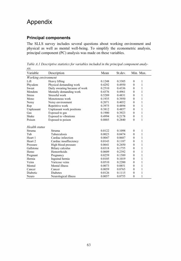
6363

Appendix

Principal components

The SLLS survey includes several questions about working environment and physical as well as mental well-being. To simplify the econometric analysis, principal component (PC) analysis was made on these variables.

Table A.1 Descriptive statistics for variables included in the principal component analy-

sis.

Variable Description Mean St.dev. Min. Max.

Working environment Lift Heavy lifting 0.1248 0.3305 0 1 Physdem Physical demanding work 0.4292 0.4950 0 1 Sweat Daily sweating because of work 0.2510 0.4336 0 1 Mendem Mentally demanding work 0.4376 0.4961 0 1 Stress Stressful work 0.5289 0.4831 0 1 Mono Monotonous work 0.1935 0.3950 0 1 Noisy Noisy environment 0.2071 0.4052 0 1 Rep Repetitive work 0.3975 0.4894 0 1 Unpleasant Unpleasant work positions 0.3812 0.4857 0 1 Gas Exposed to gas 0.1900 0.3923 0 1 Shake Exposed to vibrations 0.4994 0.2178 0 1 Poison Exposed to poison 0.0885 0.2840 0 1

Health status Struma Struma 0.0122 0.1098 0 1 Tub Tuberculosis 0.0023 0.0474 0 1 Heart 1 Cardiac infarction 0.0047 0.0687 0 1 Heart 2 Cardiac insuffieciency 0.0143 0.1187 0 1 Pressure High blood pressure 0.0641 0.2450 0 1 Gallstone Biliary calculus 0.0318 0.1755 0 1 Hemo Hemorrhoids 0.0609 0.2392 0 1 Pregnant Pregnancy 0.0259 0.1589 0 1 Hernia Inguinal hernia 0.0105 0.1019 0 1 Veins Varicose veins 0.0510 0.2200 0 1 Mental Mental illness 0.0073 0.0851 0 1 Cancer Cancer 0.0059 0.0765 0 1 Diabetic Diabetes 0.0126 0.1115 0 1 Neuro Neurological illness 0.0057 0.0755 0 1

63

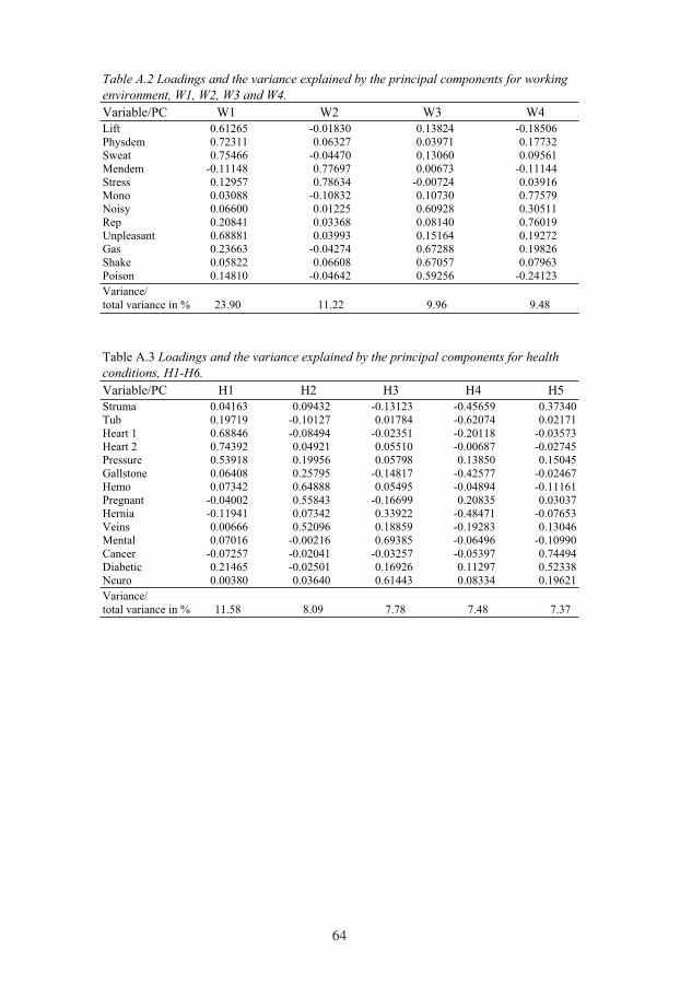
6464

Table A.2 Loadings and the variance explained by the principal components for working

environment, W1, W2, W3 and W4.

Variable/PC W1 W2 W3 W4 Lift 0.61265 -0.01830 0.13824 -0.18506 Physdem 0.72311 0.06327 0.03971 0.17732 Sweat 0.75466 -0.04470 0.13060 0.09561 Mendem -0.11148 0.77697 0.00673 -0.11144 Stress 0.12957 0.78634 -0.00724 0.03916 Mono 0.03088 -0.10832 0.10730 0.77579 Noisy 0.06600 0.01225 0.60928 0.30511 Rep 0.20841 0.03368 0.08140 0.76019 Unpleasant 0.68881 0.03993 0.15164 0.19272 Gas 0.23663 -0.04274 0.67288 0.19826 Shake 0.05822 0.06608 0.67057 0.07963 Poison 0.14810 -0.04642 0.59256 -0.24123

Variance/ total variance in % 23.90 11.22 9.96 9.48

Table A.3 Loadings and the variance explained by the principal components for health

conditions, H1-H6.

Variable/PC H1 H2 H3 H4 H5 Struma 0.04163 0.09432 -0.13123 -0.45659 0.37340 Tub 0.19719 -0.10127 0.01784 -0.62074 0.02171 Heart 1 0.68846 -0.08494 -0.02351 -0.20118 -0.03573 Heart 2 0.74392 0.04921 0.05510 -0.00687 -0.02745 Pressure 0.53918 0.19956 0.05798 0.13850 0.15045 Gallstone 0.06408 0.25795 -0.14817 -0.42577 -0.02467 Hemo 0.07342 0.64888 0.05495 -0.04894 -0.11161 Pregnant -0.04002 0.55843 -0.16699 0.20835 0.03037 Hernia -0.11941 0.07342 0.33922 -0.48471 -0.07653 Veins 0.00666 0.52096 0.18859 -0.19283 0.13046 Mental 0.07016 -0.00216 0.69385 -0.06496 -0.10990 Cancer -0.07257 -0.02041 -0.03257 -0.05397 0.74494 Diabetic 0.21465 -0.02501 0.16926 0.11297 0.52338 Neuro 0.00380 0.03640 0.61443 0.08334 0.19621

Variance/total variance in % 11.58 8.09 7.78 7.48 7.37

64

Essay III

65

Essay III

Immigrants in the Swedish sickness insur-ance system – ethnic differences in work ab-sence behavior

1 Introduction

The integration of immigrants into Swedish society has been discussed and ana-lyzed in many earlier studies. In the economic literature the focus has been on aspects such as immigrants’ labor market participation, income development and unemployment rates (Gustavsson, Zamanian & Aguilar, 1990; Ekberg & Andersson, 1995; Ekberg & Gustavsson, 1995; Gustavsson, 1997; Ekberg & Rooth, 2000; Hammarstedt, 2001; SOU 2004:21). The question concerning eco-nomic integration is growing increasingly important as the share of immigrants in Sweden increases. Today more than a tenth of the Swedish population is com-prised of immigrants. There are some empirical studies that show that immigrant workers have higher work absence rates than natives (Säll, 1968; Leinö, 1983; SOU 1989:111; Gustavsson, Zamanian & Aguilar, 1990; RFV 1990:4; Kindlund, 1995; RFV 1996:11; Akhavan & Bildt, 2004; Gustavsson & Österberg, 2004). The earlier studies are all of a descriptive and/or a cross sectional nature and their main conclusions are that absence differences to a great part can be ex-plained by differences in working situations and differences in health between immigrants and natives.1 Another important finding is that work absence not only differs between immigrants and natives but also between different groups of immigrants with women from the south of Europe being the high-risk group.

Since immigrants already are loosely attached to the labor market, high levels of work absence might lead to even greater difficulties in the process of integration. Thus, not only do immigrants have higher absence rates compared to natives, the effects of work absence might be more severe as well (Gustavsson & Östberg, 2004). If immigrants’ participation in sickness insurance systems rarely has been analyzed, there are more studies of immigrants’ utilization of other parts of the social security system. The Swedish studies are mainly concerned with immi-grants as recipients of social assistance even though there are studies of unem-ployment benefits and early retirement as well (Gustavsson, 1986; Gustavsson, Zamanian & Aguilar, 1990; Franzén, 1997; Hansen & Löfström, 2000; Ham-

––––––––– 1 There is one study using more advanced models of analysis but where immigrants are just one

among other dummy variables and where no further discussion of ethnic differences in absence fol-lows (Andrén, 2001).

65

66

marstedt, 2001; SOU 2004:21). Immigrants’ overrepresentation in public trans-fers has also been considered in cost-benefit analyses of immigration (Ekberg, 1999). Thus ethnic differences in the utilization of the social security system have been acknowledged, but the reasons for the differences are to a large part still unknown.

The higher absence rates for immigrants compared to natives may have many explanations. First, it might be due to differences in preferences. Work absence has long been analyzed within the labor supply context and is thus dependent on preferences - preferences for work (consumption) and for leisure. One factor that could explain differences in preferences is the degree of specialization within the household. In the labor supply model, a person’s labor supply is assumed to de-pend on the labor supply of the spouse. Thus the labor supply decision depends on job-sharing decisions within the family. If there are differences in job-sharing between immigrants and natives it is reasonable to expect that they will cause differences in labor supply and thus also in work absence. Differences in absence can also be the result of differences in the valuing of leisure. Second, several ear-lier studies have shown that immigrants often possess characteristics that in-crease work absence, such as poor health status and working at jobs with sub-standard working conditions (SOU 1989:111; Kindlund, 1995; Ekberg, 1996; Franzén, 1997).

The aim of this study is to analyze the background to ethnic differences in work absence. This involves two steps: First, to analyze what factors in general affect work absence behavior. An econometric model designed for modeling work ab-sence behavior accomplishes this. Second, to analyze to what extent these factors are more prevalent among immigrants or whether this group of workers acts dif-ferently on such factors (such as economic incentives, work environment or health problems). One feature attracting special attention is whether specializa-tion within the household can explain some of the ethnic differences in work ab-sence.

The analysis is based on survey data from two of the Swedish Level of Living Surveys (SLLS) which consist of interviews with a random sample of the Swed-ish population aged 16 to 74. The survey data is combined with register data from the National Social Insurance Board (NSIB) which gives us information of individual working conditions, family and economic situations, and information of annual work absences for almost 4,000 individuals. We use panel data cover-ing the period 1981 to 1991. We cannot use later data since from 1992 there is no reliable data on short-term absence at the NSIB.2 The empirical analysis is based on an econometric model derived from standard economic utility theory. The la-bor supply model is a model for daily decisions of whether to attend work or not. Considering the data generating process lead us to theoretically consistent esti-

––––––––– 2 In 1992 the responsibility for first two weeks of sick pay was transferred from NSIB to the employ-

ers.

66

67

mation methods (so-called count data models) for analyzing our annual work ab-sence data. We have detailed information of individual working conditions, fam-ily and economic situations, but there might be still other factors that influence work absence as well. We use estimation methods that can address the possibility of such unobserved heterogeneity. We also consider problems with endogeniety and we therefore estimate Negative binomial models with fixed effects.

Our analysis shows interesting ethnic differences in work absence. Not only do we find that dissimilarities in the factors affecting work absence for natives and immigrants, we also find differences in how natives and immigrants act on those factors. We find that economic incentives play a greater role in explaining work absence behavior for immigrant women than for native women. For men, we find that a poor working environment affects immigrants and natives in opposite directions. For women, we find support for the hypothesis that specialization within the household affects work absence behavior. Finally, our main result is that there are intrinsic ethnic differences in work absence. Even though we have access to exceptional rich data, the ethnic absence differences cannot be ex-plained by these observed characteristics, but rather by differences in behavior.

The paper is organized as follows: Section 2 presents the Swedish sickness in-surance system. The theoretical background is discussed and the main hypothe-ses are presented in Section 3. Section 4 presents the data and the empirical specification. The empirical results are presented Section 5 and finally, conclu-sions are discussed in Section 6.

2 The Swedish sickness insurance system

Sweden has a compulsory tax-financed national sickness insurance system ad-ministered by the National Social Insurance Board. Everyone over age 16 living in Sweden with an income over 24 percent of the base amount

3 (36,600 SEK in

year 2000) is eligible for sickness benefits if they cannot perform their regular work due to temporary health problems.

4 For the first seven days of an illness it

is up to the individual to decide whether he/she is fit for work or not. First on the eighth day of absence is a doctor’s certificate necessary. The certificate must be reviewed on the 29th day of absence and once each month for the duration of the illness.

Sickness benefits replace forgone earnings due to temporary illness up to the so-cial security ceiling of 7.5 base amounts. The replacement rate, the share of the worker’s earnings covered by sickness insurance, has been changed several times

––––––––– 3 Many of the social insurance payments are linked to the so-called base amount, which is an amount

in SEK fixed one year at a time. The base amount is political determined and has historically fol-lowed the Consumer Price Index (Palme and Svensson, 1998).

4 The unemployed and the self-employed are covered by sickness insurance but the rules differ.

67

since the introduction of the sickness insurance system in 1955. It has also varied over time as to whether the first days of a sickness spell are covered by the in-surance or not. The period we have decided to study, 1981-1991, includes two major reforms in the sickness insurance system. The regulations for the chosen period are summarized in Table 1.

Table 1. The sickness benefit system in Sweden 1981-1991. Replacement rates in percent-age of daily wage (RFV 1994, 1995, 1997). Day January 1980 December 1987 March 1, 1991 in - - - sick leave November 1987 February 1991 December 31, 1991 Replacement rate Replacement rate Replacement rate 1 0 90+10 b 65 + 10 2-3 90a 90+10 65 + 10 4-14 90 90+10 80 + 10 15-90 90 90+10 80 + 10 91-365 90 90+10 90 + 10 366- 90 90+10 90 + 10 a) The actual replacement rate was considerably lower than 90 percent. b) + 10 percent from collective agreements, for employees.

In the beginning of the 1980’s there was a qualification day (with 0 percent re-placement) which was abolished at the end of 1987. The qualification day was later reintroduced in 1993. Concurrent with the qualification day being abolished in 1987, a new way of calculating the replacement rate was introduced (“Timsjukpenningreformen”). Even though prior to this reform 90 percent of lost earnings were to be replaced, the way the calculations were made led to people actually recieving lower replacements rates. The new method of calculating re-sulted in the actual benefits being closer to 90 percent of lost earnings up to the social security ceiling. Before the reform, the daily benefit while absent was cal-culated as 90 percent of the annual income divided by 365. The problem was that benefits were only paid 5 out of 7 days per week since a standard working week does not include weekends. After the reform of 1987, the daily benefit was in-stead calculated as 90 percent of the annual income divided by the actual number of annual working days. The benefits were then paid out for those days the in-sured person was absent from work. In 1991, the replacement rates for shorter sickness spells were lowered. For the first three days of an absence spell the re-placement rate was cut to 65 percent. From day 4 through 90 in the absence spell the replacement rate was decreased to 80 percent, but from day 90 onwards it remained at 90 percent.

From the later part of the 1980’s most workers have sickness insurance in their labor union contracts in addition to the compulsory national insurance. Unfortu-nately these agreements cannot be recovered from our data.

68

69

3 Modeling work absence behavior

The choice of whether or not to attend work is not only a medical decision but also a decision depending on motivation and ability to attend work (Steers & Rhodes, 1978). At least for shorter sickness spells, going to work or not is a to-tally personal decision since it is not until the eighth day in a sickness spell that a doctor’s certificate is required for prolonged sickness benefits. From the worker’s perspective, the decision of whether or not to attend work can be ana-lyzed, on the margin, within the traditional labor supply model. The idea of modeling absenteeism with a labor supply model was first introduced by Allen (1981). The majority of all economic studies that followed after Allen’s have ei-ther explicitly or implicitly used the labor supply framework.

The traditional labor supply model states that a utility maximizing individual chooses a combination of working hours and leisure that gives him/her the great-est attainable utility. The individual is assumed to derive utility from consump-tion and leisure according to a utility function:

);,( sLxUu , (1)

where x is a bundle of consumption goods, L is leisure and s is a vector of per-sonal characteristics.

To be able to use the traditional labor supply model in the analysis of absentee-ism, we have to not only include the possibilities for the individual to work or have leisure, but also the possibility to be absent from work. This can be done by separating the leisure term, L, into two parts; contracted leisure time, lc, and time absent, la. The contracted working hours, Hc, can then be split into desired num-ber of working hours on one hand, h*, and hours of absence on the other, i.e. Hc

= h* + la. Hence we have a time constraint:

T = h* + la + lc, (2)

where T is total time available. There is also a budget constraint:

Rlhwx ac ))1(( , (3)

where w is net wage, is the replacement rate in the sickness insurance system and R is income from sources other than work. The price of the consumption goods, x, is normalized to be one. Maximizing the utility function subject to the constraints, (2) and (3), gives a demand function that can be written in the form:

);,,( sychll caa , (4)

where c is the cost of absence, c = w(1 - ), and y is virtual income when the in-dividual is absent, y = R + law .

69

70

Most of the time, work absence is a result of illness due to bad health, i.e. ab-sence is a result of low ability to attend work. Health is assumed to decrease with age and we therefore expect work absence to increase with age. There is empiri-cal support for work absence increasing with age, most often in a non-linear form with the youngest and the oldest having most absence (VandenHeuvel & Wooden, 1995; Paringer, 1983; Edgerton et. al., 1996). The age effect has in sev-eral studies been found to be stronger for men than for women. The explanation suggested by VandenHeuvel & Wooden (1995) is that women in their 30’s and 40’s often have the greatest family responsibilities, hence their absence do not decrease during those years as it does for men. The number of absence spells has however in some studies been shown to decline with age, which may be a sign of increasing work attachment or loyalty with age (Mathieu & Kohler, 1990).5 It might also be a selection process where the persons with many absence spells leave the labor market earlier than others. In several studies, immigrants have been shown to have worse health and a higher consumption of health care com-pared to natives and this might give another age absence relation than that of na-tives (Ekberg, 1996; Boalt, 1989; Kindlund 1995; Franzén, 1997; Vogel et al., 2002).

Time off from work can be seen as a time input into health production in line with the well-known Grossman model (Grossman, 1972). The individual is as-sumed to produce health with inputs of medical care and time. According to the Grossman model, a larger human capital stock increases the individual’s produc-tivity in producing health. The standard human capital variable education is sug-gested as an appropriate measure and empirically found by Grossman to increase health productivity. It is therefore natural to expect work absence to decline with education as a reflection of better health. Edgerton et. al. (1996) and Allen (1981) found that work absence decreases with education. Nevertheless, when analyzing the probability of being absent during a specific week instead of the total number of sick weeks during a year, Edgerton et. al. found no significant ef-fect of education.

Risk for poor health increases if the working situation is poor. Poor working con-ditions, mental as well as physical, do not only signify increased probability of work-related injury and illness, but also increase the marginal benefit of time off from work. A risk averse person want to minimize risk exposure given the costs. Poor working conditions would therefore be expected to increase work absence due to the resulting poor health and lowered motivation to attend work. In most studies, work absence has been shown to be strongly related to working condi-tions, both mental and physical (for example Fritzell & Lundberg, 1994; Par-inger, 1983; Barmby & Treble, 1989; Edgerton et. al., 1996; Brose, 1995). We know from earlier studies that immigrants, to a large extent, have jobs with poorer physical and mental working conditions than natives. On average, immi-

––––––––– 5 Edgerton, Kruse & Wells (1996) found on the other hand that absence frequency increased with

age.

70

71

grants have riskier, unhealthier and physically demanding jobs than natives (Leinö, 1983; RFV 1996:11). Immigrants are more often found in manufacturing and service jobs than natives although there are differences between immigrants; women from the south of Europe possess the most unhealthy work environments (RFV 1996:11).

In the traditional labor supply model time can be used either for work or for lei-sure. An alternative use would be home production in the sense of Gronau (1986) where the input of time is as important in the production of commodities as in the input of market goods is. All factors that increase the marginal utility of time spent in home production should also, ceteris paribus, increase the willing-ness to be absent from work. Pressing family responsibilities, conditioned on working time, would increase the total pressure from home and market produc-tion on a person; high pressure may bring about lower well-being and thereby higher absence. The pressure of family responsibility is, of course, even greater if the individual is a lone parent.

Family responsibility does not only depend on characteristics such as whether a person is married or not or how many children there are in the family. It also has to do with job-sharing decisions within the family or with specialization within the household, as Becker (1965) formulates it. Over time, gender equality has in-creased in Sweden and today Swedish women are among the ones most equal to men in several aspects. Yet, research shows women still have the greatest re-sponsibility for family and the highest degree of time spent on home production (Flood & Gråsjö, 1997; Anxo & Flood, 1997). Even if it is a kind of stereotype, it is true that many immigrants come from countries with more traditional gender roles than Sweden (SOU 1979:89). It is reasonable to assume that at least in the beginning of their lives in Sweden, immigrants stick to their traditions with women undertaking even greater family responsibility than Swedish women. Empirical studies have shown that the position of the woman in a family also de-pends on social and economic status (Darvishpour, 1997).

A part-time job means more time off from work and also lowers total work pres-sure, i.e. the combined pressure from home and market production.

6 This would

mean, ceteris paribus, that part-time workers can be expected to have less use of absence as a device for recieving extra time off for home production, as well as greater well-being due to lower pressure. This is supported by several earlier studies where working part-time has been found to decrease work absence (Edgerton et. al., 1996; Chaudhury & Ng, 1992; Drago & Wooden, 1992). It should be considered that the choice of whether or not to work part-time might not be voluntary. Individuals who voluntarily choose to work part-time probably have a higher marginal benefit of time off from work than those who want a full-

––––––––– 6 There are several studies showing that women do not cut down on home production when they in-

crease their market production, at least not in the same proportion (see for example Flood & Gråsjö, 1997).

71

72

time job but are only offered a part-time job. The same holds true for those who choose to work full-time in contrast to those who are forced to do so. Those forced to work full-time probably have a higher marginal benefit of time off from work and therefore higher absence than those who have voluntarily chosen full-time.

In earlier studies, immigrants have been shown to work full-time to a greater ex-tent than natives; especially for women, there is a distinct difference in the share with full-time versus part-time jobs between immigrants and natives (Leinö, 1983; Ekberg, 1999). Kindlund (1995) discusses the importance of the reason for immigration. If the goal is to return to the country of origin, immigrants might organize their lives to accomplish as great savings as possible in as short a time as possible. In the short run this might encourage a high degree of overloading, especially for the women in the family, i.e. working full time yet still with the main responsibility for the family.

Working nighttime or having shift-work have often been found to cause health problems (Dagens Medicin 1999, 2000). On the other hand, it is reasonable to assume that such workers experience greater flexibility in their daily lives and have more time available for home production. This would imply that they are likely to make less use of absence as a device for achieving flexibility. Vanden-Heuvel & Wooden (1995) formulates a hypothesis the other way around. Those who work in the evenings are more likely than non-shift workers to have family matters overlapping with their work time; it is more pronounced for women who have a greater family responsibility than men. Thus, whether shift/night-time work increases or decreases work absence is left to the empirical analysis. Björklund (1991) found that female shift workers have more absent days com-pared to their other female colleagues while male shift workers have lower ab-sence compared to other men which is the same result as in VandenHeuvel &Wooden (1995).

The pecuniary cost of absence, c in the demand function (4), is the net earnings not covered by sickness insurance, which depends both on the wage rate and the replacement rate within the sickness insurance system. Wage, w, has an ambigu-ous effect on work absence due to the conflicting substitution and income ef-fects. A higher wage means a higher cost of absence, but at the same time a higher wage implies higher income, which make it more affordable to be absent. Wages also have a more indirect relation with absence, which may create prob-lems with endogeniety. Workers with poor health usually have more work ab-sence than workers with no health problems. For some jobs then, it is reasonable to assume that workers with poor health are less productive and therefore earn less than those with good health. There might also be persons that are more pro-ne to absence than others and therefore receive less pay since they have less on-the-job training. Absence and wages may also be correlated in line with the the-ory of compensating wage differentials (Rosen, 1986). The worker may accept higher risks at work in exchange for a higher wage. Yet another reason for corre-lation between absence and wages is due to the use of efficiency wages (Shapiro

72

73

& Stiglitz, 1984). Through paying higher wages, employers may encourage workers to attend work. These relations between work absence and wages all make the effect of wages on absence harder to estimate. A negative relation be-tween work absence and the wage rate has been found, however, in several ear-lier studies (Drago & Wooden, 1992; Chaudhury & Ng, 1992; Edgerton et. al., 1996; Winkelmann, 1999).

The impact of sickness benefit, , is on the other hand unambiguous since the in-come and substitution effects go in the same direction. The temptation to use ab-sence as a device to reach the optimal combination of work and leisure increases when the cost of being absent is lowered. As in all labor supply models a per-son’s unearned income can be expected to affect the time allocation decision. An increase in unearned income, R, has only an income effect and we can therefore expect work absence to increase with unearned income. Several earlier studies have shown a strong relationship between economic incentives and work ab-sence (Allen, 1981; Barmby, Orme & Treble, 1995; Johansson & Palme, 1996, 2002; Henrekson & Persson, 2004).

Workers’ absence behavior not only affects the insuring authority but of course also the employers.

7 The employer can make it more costly for the workers to be

absent from work by using different kinds of penalties, such as decreased prob-ability of receiving promotion or merit wage increases and/or an increased likeli-hood of being dismissed (Allen, 1981).

8 It might also pay off for the employer to

control the workers through different kinds of monitoring devices, although this can be difficult since illness is private information.

Work absence has most often been found to have a negative relation with unem-ployment (Henrekson, Lantto & Persson, 1992; Leigh, 1985; Lantto & Lind-blom, 1987; Chaudhury & Ng, 1992; Drago & Wooden, 1992; Johansson & Palme, 1996; Arai & Skogman Thoursie, 2005). The explanations are based on disciplining effects and composition theories. The cost of losing the job is higher in times of high unemployment, which make people more disciplined. People with poor health are mainly the ones that leave or do not enter the labor market when unemployment is high. But it is not unreasonable to consider that there could also be effects in the opposite direction. High unemployment can in itself cause poor health, both for the unemployed and for people who are employed but worried about losing their jobs (Bäckman, 1998; Östlin et al., 1996). So theoreti-cally, we cannot say whether unemployment increases or decreases work ab-

––––––––– 7 Even more so after the reform in 1992 when the employer were made responsible for portions of the

sick pay. 8 The effect of penalties could be expected to differ between different age groups and between differ-

ent occupations according to tournament theory and work life incentive theory as Lazear (1999) formulates them.

73

74

sence. Though the labor market situation differs for different kinds of immi-grants (refugees, labor force immigrants or other immigrants), the overall pattern during the period shows that the labor market situation is more difficult for im-migrants than for natives (Gustavsson, Zamanian & Aguilar, 1990; Ekberg & Andersson, 1995; Ekberg & Gustavsson, 1995; Gustavsson, 1997). This might of course affect absence behavior of immigrants both in terms of a more severe dis-ciplining effect and selection of those who actually get jobs.

4 Data and empirical specification

We use survey data from the Swedish Level of Living Survey (SLLS) combined with register data from the National Social Insurance Board (NSIB). The survey is a panel that covers a random sample of approximately 7,000 individuals aged between 16 and 74, of which around 600 are immigrants. The individuals are in-terviewed about their working situations as well as personal and economic situa-tions (See Fritzell & Lundberg, 1994, for a detailed description of the surveys). The surveys have been undertaken five times during the last five decades, but we only use information from the two surveys undertaken in 1981 and 1991. The absence register data from NSIB that we use includes information about all ab-sence spells during the period 1981-1991 for the individuals interviewed in the SLLS surveys.

4.1 Sampling procedure

Our data has a panel structure where 6,985 individuals were interviewed in 1981 and 6,773 in 1991. Since we focus on absence in the sense of being absent from work, we concentrate on people of working age 20 to 64 years old. The 6,570 in-dividuals between the ages of 20 and 64 included in either the 1981 and/or the 1991 surveys are then further reduced according to the sampling procedure summarized in Table 2. Since one aspect to be analyzed is the effect on work ab-sence by the working situation, we want to ensure that the sampled individuals actually have jobs. Thus we exclude those who do not have part-time or full-time jobs during the period studied. The sample is further reduced since some had missing values for some variables and some had miscoded age variables. This sampling procedure leaves us with an unbalanced panel including 3,804 indi-viduals of which 501 are immigrants.

Table 2. Sample construction.

No. of people in the 1981 SLLS 6,985 No. of people in the 1981 SLLS, aged 20-64 5,363 No. of people in the 1991 SLLS 6,773 No. of people in the 1991 SLLS, aged 20-64 4,298 No. of people aged 20-64 in the 1981 and the 1991 SLLS, totally 6,570 No. of people with a part-time/full-time job of the above 3,913 No. of people after excluding those with missing values/miscoded variables 3,804

74

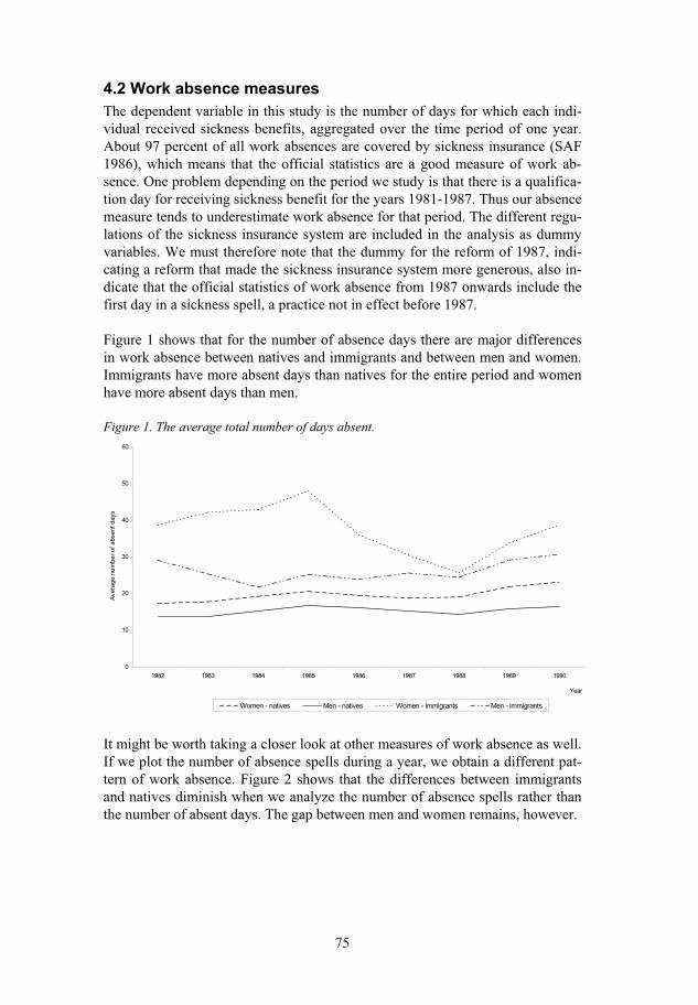
75

4.2 Work absence measures

The dependent variable in this study is the number of days for which each indi-vidual received sickness benefits, aggregated over the time period of one year. About 97 percent of all work absences are covered by sickness insurance (SAF 1986), which means that the official statistics are a good measure of work ab-sence. One problem depending on the period we study is that there is a qualifica-tion day for receiving sickness benefit for the years 1981-1987. Thus our absence measure tends to underestimate work absence for that period. The different regu-lations of the sickness insurance system are included in the analysis as dummy variables. We must therefore note that the dummy for the reform of 1987, indi-cating a reform that made the sickness insurance system more generous, also in-dicate that the official statistics of work absence from 1987 onwards include the first day in a sickness spell, a practice not in effect before 1987.

Figure 1 shows that for the number of absence days there are major differences in work absence between natives and immigrants and between men and women. Immigrants have more absent days than natives for the entire period and women have more absent days than men.

Figure 1. The average total number of days absent.

0

10

20

30

40

50

60

1982 1983 1984 1985 1986 1987 1988 1989 1990

Year

Ave

rag

e n

um

be

r o

f a

bse

nt

da

ys

Women - natives Men - natives Women - immigrants Men - immigrants

It might be worth taking a closer look at other measures of work absence as well. If we plot the number of absence spells during a year, we obtain a different pat-tern of work absence. Figure 2 shows that the differences between immigrants and natives diminish when we analyze the number of absence spells rather than the number of absent days. The gap between men and women remains, however.

75

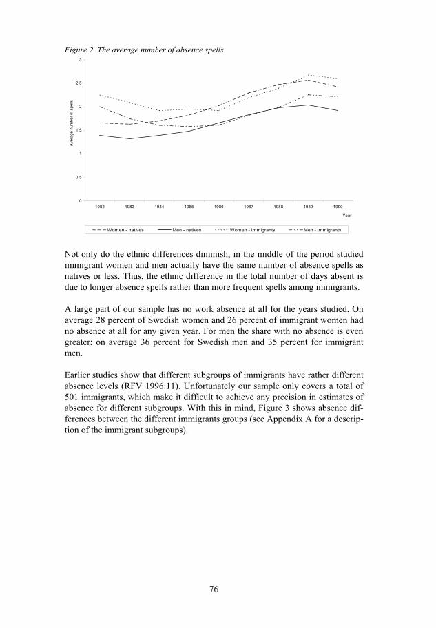
76

Figure 2. The average number of absence spells.

0

0,5

1

1,5

2

2,5

3

1982 1983 1984 1985 1986 1987 1988 1989 1990

Year

Avera

ge n

um

ber

of

spells

Women - natives Men - natives Women - immigrants Men - immigrants

Not only do the ethnic differences diminish, in the middle of the period studied immigrant women and men actually have the same number of absence spells as natives or less. Thus, the ethnic difference in the total number of days absent is due to longer absence spells rather than more frequent spells among immigrants.

A large part of our sample has no work absence at all for the years studied. On average 28 percent of Swedish women and 26 percent of immigrant women had no absence at all for any given year. For men the share with no absence is even greater; on average 36 percent for Swedish men and 35 percent for immigrant men.

Earlier studies show that different subgroups of immigrants have rather different absence levels (RFV 1996:11). Unfortunately our sample only covers a total of 501 immigrants, which make it difficult to achieve any precision in estimates of absence for different subgroups. With this in mind, Figure 3 shows absence dif-ferences between the different immigrants groups (see Appendix A for a descrip-tion of the immigrant subgroups).

76

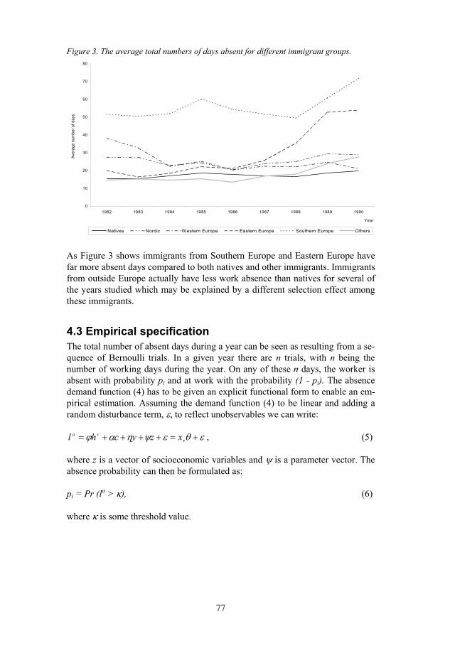
77

Figure 3. The average total numbers of days absent for different immigrant groups.

0

10

20

30

40

50

60

70

80

1982 1983 1984 1985 1986 1987 1988 1989 1990

Year

Ave

rag

e n

um

be

r o

f d

ays

Natives Nordic W estern Europe Eastern Europe Southern Europe Others

As Figure 3 shows immigrants from Southern Europe and Eastern Europe have far more absent days compared to both natives and other immigrants. Immigrants from outside Europe actually have less work absence than natives for several of the years studied which may be explained by a different selection effect among these immigrants.

4.3 Empirical specification

The total number of absent days during a year can be seen as resulting from a se-quence of Bernoulli trials. In a given year there are n trials, with n being the number of working days during the year. On any of these n days, the worker is absent with probability pi and at work with the probability (1 - pi). The absence demand function (4) has to be given an explicit functional form to enable an em-pirical estimation. Assuming the demand function (4) to be linear and adding a random disturbance term, , to reflect unobservables we can write:

xzychl ca , (5)

where z is a vector of socioeconomic variables and is a parameter vector. The absence probability can then be formulated as:

pi = Pr (la > ), (6)

where is some threshold value.

77

78

If the n Bernoulli variables, Xn, is summed over one year we get the total number of absent days during a specific year, t, for individual, i:

N

n

itnitXY

1

, (7)

The total number of absent days, Yit, can be shown to be Poisson distributed with expected value and variance equal to it as n tends to infinity if the Bernoulli tri-als are assumed to be independent and that the probability pi = it / n is constant. The probability that the number of days during a year will be equal to yit, can then be written as:

!)(

it

y

it

itity

eyYprob

itit

, where yit = 0, 1, 2, 3…. (8)

Let the expected value of Yit, it, be a deterministic function of the covariates:

'lnitit

x , (9)

where xit is the (1 k) vector of exogenous explanatory variables for individual iat time t. is the corresponding unknown parameter vector we want to estimate and the exponential form ensures non-negativity of it.

The log likelihood function is given by:

n

i

itititit

T

t

yyL11

!lnlnln . (10)

The problem with the Poisson model is that it does not allow for overdispersion, which could be expected in our kind of data (Johansson & Brännäs, 1998). Both violation of the independence assumption, that absence in (t) does not depend on absence in (t – 1), and unobserved heterogeneity result in a situation in which the variance exceeds the mean. Following Hausman, Hall & Griliches (1984), in-stead of assuming that it is constant, we can assume that it follows a gamma distribution with parameters ( it, ) and specify:

'lnitit

x , (11)

with common both across individuals and across time. With this specification,Yit follows a negative binomial distribution with parameters ( it, ) which gives:

ity

it

it

itit

it

itity

yyYprob

)1()(

)()( . (12)

78

79

For this model, E[Yit] = it and Var(Yit) = E[Yit] + (E[Yit])2 where = 1/ and

thus the specification allows for overdispersion with the original Poisson as a limiting case as . This is the model called Negbin II in Cameron & Trivedi (1986).

We have annual individual data over an eleven-year period. So far the models have not allowed for any correlation over time between the absences of a specific individual. It is reasonable to believe that there are some unobserved individual-specific effects. This would mean that some individuals are on average always above/under the average absence level. In order to add individual specific effects we consider both a fixed and a random effects specification. A conditional max-imum likelihood approach is used to derive the former. The resulting joint prob-ability for an individual’s absence conditional on the eleven year total is the fol-lowing:

t t

itit

t t

itit

t itit

itit

itiTi

y

y

y

yYYYprob

)(

)1()(

1)()(

)()|,...,( 1 . (13)

We set the parameters of the underlying model to:

)/,(),( iit eei

x

iit, (14)

where both i

andiare allowed to vary across individuals. The Negative bi-

nomial model with fixed effects then allows for overdispersion as well as for an individual specific variance to the mean ratio. The random effects model intro-duces randomness both across individuals and across time by assuming that

iu

ie/ is randomly distributed across individuals, independent of the xit’s. Fol-

lowing Hausman, Hall & Griliches (1984), we assume:

i

i

1 beta (a, b), (15)

where a and b are to be estimated. Integrating, using this density, will result in the following joint probability function for individual i:

t itit

itit

t t

itit

t t

itit

iTitiTiy

y

ybaba

ybaba

xxYYprob)1()(

)(

)()()(

)()()(),...,|,...,( 1 . (16)

79

80


The demand function (4) shows that work absence depends on contracted work-ing hours, cost of absence, virtual income and a set of socioeconomic variables. To be able to consider working conditions as well as the personal and economic situations, several independent variables have been constructed out of the survey answers. We have data on the individuals’ absence for every single year between 1981 and 1991, but unfortunately we do not know anything about their working situation between these years. Therefore we assume that the personal, economic and working situation for the years 1982-1986 is the same as in 1981 and that the situation for the years 1987-1990 is the same as in 1991. This is a fairly strong assumption but to be able to use the rich data on work absence this is the only available solution. The variables used in the analysis are summarized in Table 3.

Personal characteristics considering family situation and education level are in-cluded since they are expected to influence the ability and the motivation to at-tend work. Married, kids, small kids and the education variables, high school and university, are all dummy variables. They indicate whether a person is married or cohabiting, has children above the age of 6 living at home, has small children (< 6 years old) living at home and whether the highest level of education is a high school degree or a university degree.

Several variables reflecting the working situation are included. Income is the hourly wage, deflated by the Consumer Price Index with 1980 as the base year, used as a control for the opportunity cost of absence. Two reform dummies, ref87 and ref91, are also included in the analysis to reflect changes in the sick-ness insurance system and thus changes in the cost of absence. Unfortunately, we have no variable measuring virtual income due to measurement problems. Previ-ous studies such as Johansson & Palme (2002) have reported problems with measuring income and obtained relatively low precision in their estimates. Part-

time is a dummy variable included as a proxy for contracted working hours andshift indicates whether a person works shift or not. Shorter is a dummy variable indicating if the person wants to work fewer hours and serves as an indicator for the person’s valuing of consumption versus leisure. This follows the discussion in Dunn & Youngblood (1986) of work absence as a response to non-optimal la-bor market equilibrium.

One important aspect of the socio-economic variables is of course the state of health. The SLLS surveys contain several questions concerning health. We have picked a set of 14 variables, for which a physician has most likely made a diag-nosis, and which are not strongly affected by poor working conditions. We are only interested in controlling for differences in health status therefore we have constructed a health dummy, H, which takes the value one if a person has any of the 14 diagnoses and 0 otherwise. The fourteen diagnoses are presented in Ap-pendix B.

80

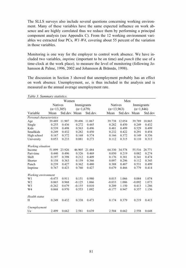
81

The SLLS surveys also include several questions concerning working environ-ment. Many of these variables have the same expected influence on work ab-sence and are highly correlated thus we reduce them by performing a principal component analysis (see Appendix C). From the 12 working environment vari-ables we extracted four PCs, W1-W4, covering about 55 percent of the variation in those variables.

Monitoring is one way for the employer to control work absence. We have in-cluded two variables, imptime (important to be on time) and punch (the use of a time-clock at the work place), to measure the level of monitoring (following Jo-hansson & Palme, 1996, 2002 and Johansson & Brännäs, 1998).

The discussion in Section 3 showed that unemployment probably has an effect on work absence. Unemployment, ue, is thus included in the analysis and is measured as the annual average unemployment rate.

Table 3. Summary statistics.

Women Men Natives Immigrants Natives Immigrants (n=13,305) (n=1,679) (n=13,963) (n=1,846) Variable Mean Std.dev. Mean Std.dev. Mean Std.dev. Mean Std.dev Personal characteristics

Age 39.489 11.907 39.496 11.067 39.738 12.054 39.789 10.865 Single 0.255 0.436 0.272 0.445 0.282 0.450 0.249 0.432 Kids 0.539 0.498 0.563 0.496 0.481 0.499 0.529 0.499 Smallkids 0.249 0.432 0.282 0.450 0.232 0.422 0.291 0.454 High school 0.167 0.372 0.168 0.374 0.166 0.372 0.149 0.356 University 0.053 0.233 0.081 0.273 0.112 0.315 0.110 0.313 Working situation

Income 51.899 23.926 46.905 21.484 64.330 34.578 55.516 28.771 Part-time 0.440 0.496 0.326 0.469 0.050 0.219 0.082 0.274 Shift 0.197 0.398 0.212 0.409 0.176 0.381 0.341 0.474 Shorter 0.158 0.363 0.159 0.366 0.097 0.296 0.112 0.345 Punch 0.239 0.427 0.362 0.480 0.388 0.487 0.531 0.499 Imptime 0.767 0.423 0.760 0.427 0.679 0.466 0.779 0.414

Working environment

W1 -0.475 0.911 0.151 0.980 0.015 1.066 0.084 1.074 W2 0.065 0.968 -0.125 1.066 -0.033 1.006 -0.092 1.073 W3 -0.262 0.679 -0.155 0.810 0.209 1.150 0.413 1.286 W4 0.068 0.970 0.553 1.092 -0.177 0.947 0.357 1.156 Health status

H 0.249 0.432 0.338 0.473 0.174 0.379 0.219 0.413

Unemployment

Ue 2.499 0.662 2.581 0.639 2.504 0.662 2.558 0.648

81

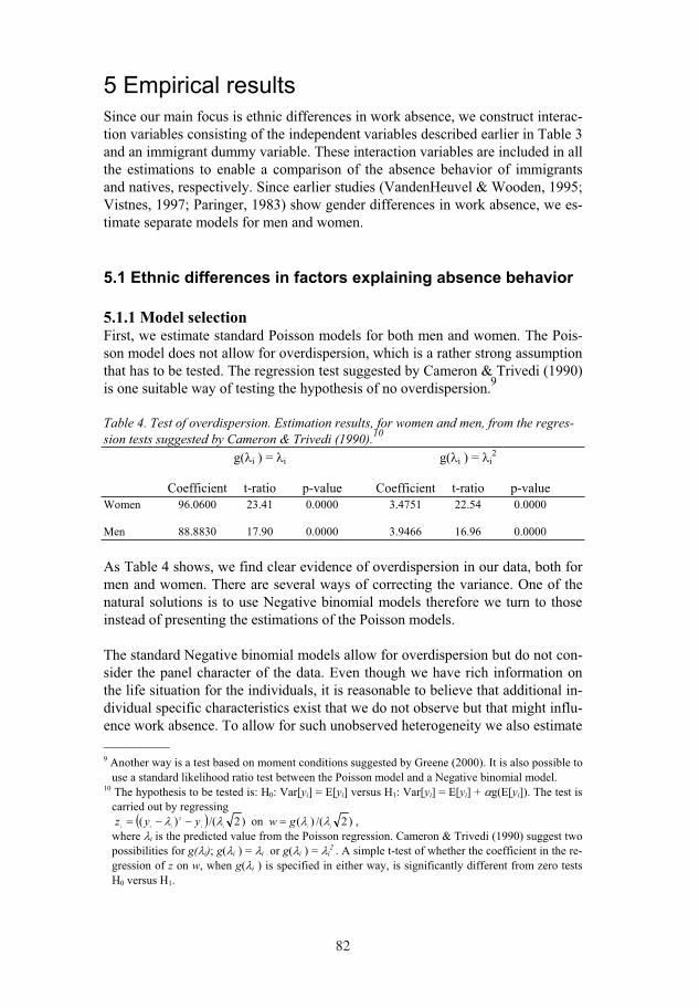
82

5 Empirical results

Since our main focus is ethnic differences in work absence, we construct interac-tion variables consisting of the independent variables described earlier in Table 3 and an immigrant dummy variable. These interaction variables are included in all the estimations to enable a comparison of the absence behavior of immigrants and natives, respectively. Since earlier studies (VandenHeuvel & Wooden, 1995; Vistnes, 1997; Paringer, 1983) show gender differences in work absence, we es-timate separate models for men and women.

5.1 Ethnic differences in factors explaining absence behavior

5.1.1 Model selection First, we estimate standard Poisson models for both men and women. The Pois-son model does not allow for overdispersion, which is a rather strong assumption that has to be tested. The regression test suggested by Cameron & Trivedi (1990) is one suitable way of testing the hypothesis of no overdispersion.

9


sion tests suggested by Cameron & Trivedi (1990).10

g( i ) = i g( i ) = i2

Coefficient t-ratio p-value Coefficient t-ratio p-value Women 96.0600 23.41 0.0000 3.4751 22.54 0.0000

Men 88.8830 17.90 0.0000 3.9466 16.96 0.0000

As Table 4 shows, we find clear evidence of overdispersion in our data, both for men and women. There are several ways of correcting the variance. One of the natural solutions is to use Negative binomial models therefore we turn to those instead of presenting the estimations of the Poisson models.

The standard Negative binomial models allow for overdispersion but do not con-sider the panel character of the data. Even though we have rich information on the life situation for the individuals, it is reasonable to believe that additional in-dividual specific characteristics exist that we do not observe but that might influ-ence work absence. To allow for such unobserved heterogeneity we also estimate

––––––––– 9 Another way is a test based on moment conditions suggested by Greene (2000). It is also possible to

use a standard likelihood ratio test between the Poisson model and a Negative binomial model. 10 The hypothesis to be tested is: H0: Var[yi] = E[yi] versus H1: Var[yi] = E[yi] + g(E[yi]). The test is


iiiiiyyz on )2/()(

iigw ,

where i is the predicted value from the Poisson regression. Cameron & Trivedi (1990) suggest two possibilities for g( i); g( i ) = i or g( i ) = i

2 . A simple t-test of whether the coefficient in the re-gression of z on w, when g( i ) is specified in either way, is significantly different from zero tests H0 versus H1.

82

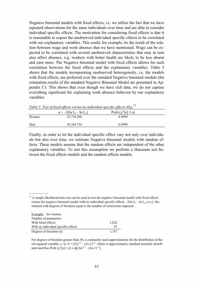
83

Negative binomial models with fixed effects, i.e. we utilize the fact that we have repeated observations for the same individuals over time and are able to consider individual specific effects. The motivation for considering fixed effects is that it is reasonable to expect the unobserved individual specific effects to be correlated with our explanatory variables. This could, for example, be the result of the rela-tion between wage and work absence that we have mentioned. Wage can be ex-pected to be correlated with several unobserved characteristics that may in turn also affect absence, e.g. workers with better health are likely to be less absent and earn more. The Negative binomial model with fixed effects allows for such correlation between the fixed effects and the explanatory variables. Table 5 shows that the models incorporating unobserved heterogeneity, i.e. the models with fixed effects, are preferred over the standard Negative binomial models (the estimation results of the standard Negative Binomial Model are presented in Ap-pendix C). This shows that even though we have rich data, we do not capture everything significant for explaining work absence behavior by our explanatory variables.

Table 5. Test of fixed effects versus no individual specific effects (H0).11

a = –2(ln Lr – ln Lu) Prob ( 2[n] a) Women 25,770.368 0.9999

Men 26,364.734 0.9999

Finally, in order to let the individual specific effect vary not only over individu-als but also over time, we estimate Negative binomial models with random ef-fects. These models assume that the random effects are independent of the other explanatory variables. To test this assumption we perform a Hausman test be-tween the fixed effects models and the random effects models.

––––––––– 11 A simple likelihood ratio test can be used to test the negative binomial model with fixed effects

versus the negative binomial model with no individual specific effects. -2(ln Lr – ln Lur) is 2 dis-tributed with degrees of freedom equal to the number of restrictions imposed.

Example – for women. Number of parameters

With fixed effects 1,822 With no individual specific effects 55

Degrees of freedom (n) 1,767

For degrees of freedom greater than 30, a commonly used approximation for the distribution of the chi-squared variable, x, is: Z = (2x)1/2 – (2n-1)1/2 which is approximately standard normally distrib-uted and thus Prob ( 2[n] a) [(2a)1/2 – (2n-1)1/2].

83

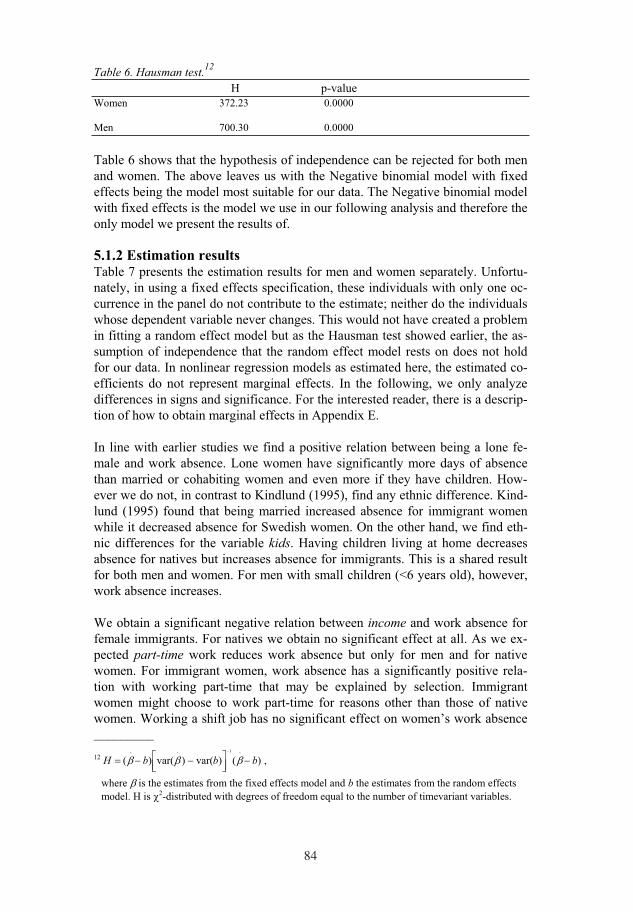
84

Table 6. Hausman test.12

H p-value Women 372.23 0.0000

Men 700.30 0.0000

Table 6 shows that the hypothesis of independence can be rejected for both men and women. The above leaves us with the Negative binomial model with fixed effects being the model most suitable for our data. The Negative binomial model with fixed effects is the model we use in our following analysis and therefore the only model we present the results of.

5.1.2 Estimation results Table 7 presents the estimation results for men and women separately. Unfortu-nately, in using a fixed effects specification, these individuals with only one oc-currence in the panel do not contribute to the estimate; neither do the individuals whose dependent variable never changes. This would not have created a problem in fitting a random effect model but as the Hausman test showed earlier, the as-sumption of independence that the random effect model rests on does not hold for our data. In nonlinear regression models as estimated here, the estimated co-efficients do not represent marginal effects. In the following, we only analyze differences in signs and significance. For the interested reader, there is a descrip-tion of how to obtain marginal effects in Appendix E.

In line with earlier studies we find a positive relation between being a lone fe-male and work absence. Lone women have significantly more days of absence than married or cohabiting women and even more if they have children. How-ever we do not, in contrast to Kindlund (1995), find any ethnic difference. Kind-lund (1995) found that being married increased absence for immigrant women while it decreased absence for Swedish women. On the other hand, we find eth-nic differences for the variable kids. Having children living at home decreases absence for natives but increases absence for immigrants. This is a shared result for both men and women. For men with small children (<6 years old), however, work absence increases.

We obtain a significant negative relation between income and work absence for female immigrants. For natives we obtain no significant effect at all. As we ex-pected part-time work reduces work absence but only for men and for native women. For immigrant women, work absence has a significantly positive rela-tion with working part-time that may be explained by selection. Immigrant women might choose to work part-time for reasons other than those of native women. Working a shift job has no significant effect on women’s work absence

––––––––– 12 )()var()var()(

^1

^^

bbbH ,

where is the estimates from the fixed effects model and b the estimates from the random effects model. H is 2-distributed with degrees of freedom equal to the number of timevariant variables.

84

85

while it decreases absence for native men and increases absence for immigrant men. This might has to do with selection as well. The only support for work ab-sence as a response to non-optimal labor market equilibrium is found for men by a significant parameter estimate for the variable shorter. There seems to be no ethnic difference in this aspect.

Several of the work environment characteristics get the expected parameter esti-mates. A poor working environment significantly increases work absence for both men and women, but there seems to be a pronounced ethnic difference for men. We actually obtain significantly negative estimates for immigrant men that might be explained by selection effects. It is possible that healthier immigrant men with lower absence choose to work in poor work environments – the so-called healthy worker effect. Selection effects may also explain why immigrants do not have the same relation between absence and the level of health. In our es-timations, it is only for native men that the health dummy gets a significant posi-tive parameter estimate. Immigrants rather seem to have less absence if any of the 14 diagnoses is present.

The reform of 1987 that increased the benefits had a significantly positive effect on the number of absent days for both men and women. For immigrants the ef-fect was even stronger. It appears as immigrant women are more sensitive to eco-nomic incentives than native women. Their work absence is more strongly re-lated to income and benefit levels than absence for native women. Surprisingly, the reform of1991, that markedly reduced benefits, also increases work absence for men as well as for women. This might be explained by our measure of work absence. The reform of 1991 made short-term absences more costly, thus affect-ing the number of absence spells rather than the total number of absent days. Jo-hansson & Palme (1996) found that short-term spells dropped between 1990 and 1991 while longer spells actually increased. Finally, we obtain the expected counter-cyclical relation between work absence and unemployment, but do not find any ethnic differences in this aspect.

85

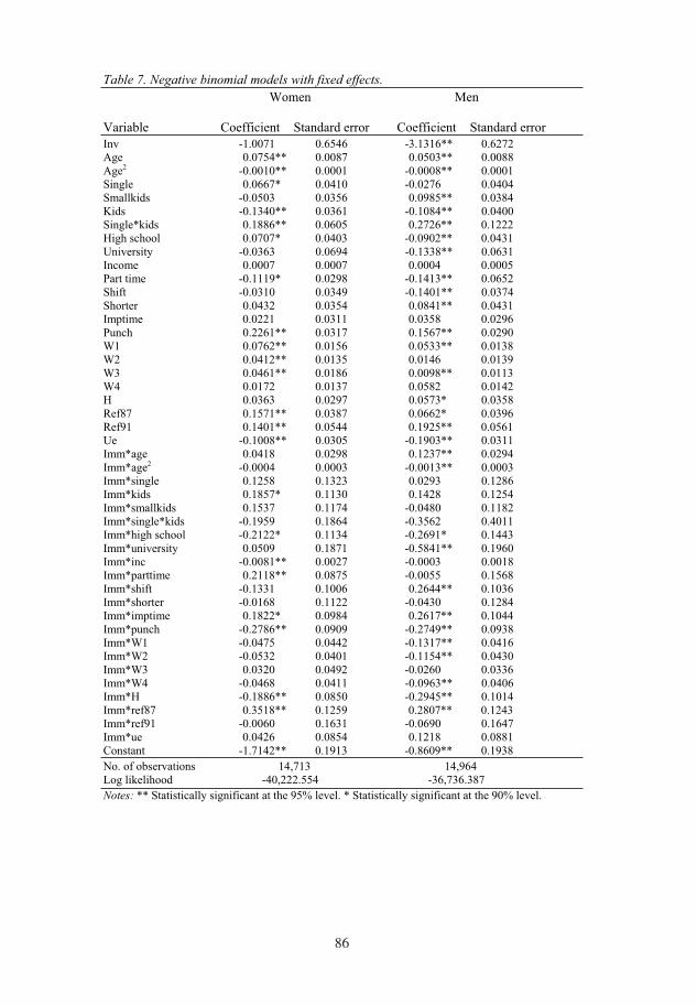
86

Table 7. Negative binomial models with fixed effects.

Women Men

Variable Coefficient Standard error Coefficient Standard error Inv -1.0071 0.6546 -3.1316** 0.6272 Age 0.0754** 0.0087 0.0503** 0.0088 Age2 -0.0010** 0.0001 -0.0008** 0.0001 Single 0.0667* 0.0410 -0.0276 0.0404 Smallkids -0.0503 0.0356 0.0985** 0.0384 Kids -0.1340** 0.0361 -0.1084** 0.0400 Single*kids 0.1886** 0.0605 0.2726** 0.1222 High school 0.0707* 0.0403 -0.0902** 0.0431 University -0.0363 0.0694 -0.1338** 0.0631 Income 0.0007 0.0007 0.0004 0.0005 Part time -0.1119* 0.0298 -0.1413** 0.0652 Shift -0.0310 0.0349 -0.1401** 0.0374 Shorter 0.0432 0.0354 0.0841** 0.0431 Imptime 0.0221 0.0311 0.0358 0.0296 Punch 0.2261** 0.0317 0.1567** 0.0290 W1 0.0762** 0.0156 0.0533** 0.0138 W2 0.0412** 0.0135 0.0146 0.0139 W3 0.0461** 0.0186 0.0098** 0.0113 W4 0.0172 0.0137 0.0582 0.0142 H 0.0363 0.0297 0.0573* 0.0358 Ref87 0.1571** 0.0387 0.0662* 0.0396 Ref91 0.1401** 0.0544 0.1925** 0.0561 Ue -0.1008** 0.0305 -0.1903** 0.0311 Imm*age 0.0418 0.0298 0.1237** 0.0294 Imm*age2 -0.0004 0.0003 -0.0013** 0.0003 Imm*single 0.1258 0.1323 0.0293 0.1286 Imm*kids 0.1857* 0.1130 0.1428 0.1254 Imm*smallkids 0.1537 0.1174 -0.0480 0.1182 Imm*single*kids -0.1959 0.1864 -0.3562 0.4011 Imm*high school -0.2122* 0.1134 -0.2691* 0.1443 Imm*university 0.0509 0.1871 -0.5841** 0.1960 Imm*inc -0.0081** 0.0027 -0.0003 0.0018 Imm*parttime 0.2118** 0.0875 -0.0055 0.1568 Imm*shift -0.1331 0.1006 0.2644** 0.1036 Imm*shorter -0.0168 0.1122 -0.0430 0.1284 Imm*imptime 0.1822* 0.0984 0.2617** 0.1044 Imm*punch -0.2786** 0.0909 -0.2749** 0.0938 Imm*W1 -0.0475 0.0442 -0.1317** 0.0416 Imm*W2 -0.0532 0.0401 -0.1154** 0.0430 Imm*W3 0.0320 0.0492 -0.0260 0.0336 Imm*W4 -0.0468 0.0411 -0.0963** 0.0406 Imm*H -0.1886** 0.0850 -0.2945** 0.1014 Imm*ref87 0.3518** 0.1259 0.2807** 0.1243 Imm*ref91 -0.0060 0.1631 -0.0690 0.1647 Imm*ue 0.0426 0.0854 0.1218 0.0881 Constant -1.7142** 0.1913 -0.8609** 0.1938

No. of observations 14,713 14,964 Log likelihood -40,222.554 -36,736.387

Notes: ** Statistically significant at the 95% level. * Statistically significant at the 90% level.

86

87

5.2 Ethnic differences in predicted number of absent days

The estimated models have shown not only which factors affect work absence, but also that there are differences in how immigrants and natives act on those factors, i.e. there are differences not only in characteristics but also in the re-sponse to these characteristics.

In order to gain a sense of the extent that that different characteristics affect na-tives’ and immigrants’ work absence, i.e. how the differences in preferences af-fect absence levels, we perform simulations. We analyze what happens with the predicted number of absent days for immigrants if we change some of the char-acteristics (independent variables) to make them resemble the characteristics of natives. To be able to obtain predicted values, we have to, following Blonigen (1997), abandon the individual specific effects that are considered in the Nega-tive binomial models with fixed effects and instead use the standard Negative bi-nomial model on the pooled sample. It is of course, a simplification since we previously showed that there are important influences of unobserved individual effects, but it is the only way to achieve closed forms solutions. In the Negative binomial model with fixed effects the group effects are conditioned out, and not computed, therefore it is impossible to obtain predicted values. Keeping this in mind it might still be interesting to run simulations to gain a sense of the magni-tudes of the effects - we just have to be cautious when analyzing the results.

Thus, we first estimate the predicted number of absent days for natives and im-migrants respectively using the parameter estimates from the standard Negative binomial models (see Appendix D). Table 8 shows that there are considerable differences in the number of predicted absent days between natives and immi-grants as well as between men and women. Immigrants have almost twice as many absent days as natives. The gender gap in work absence is greater for im-migrants than for natives. Immigrant women have on average about 15 days more absence compared to immigrant men while native women on average only have about 4 days more absence compared to native men.

Table 8 also shows what happens with the predicted number of absent days for immigrants if we make changes in different characteristics. We replace the true values for certain variables for immigrants with the mean of the corresponding variables for natives. This kind of simulation is done for variables measuring personal characteristics, working situation, working environment and health sta-

tus as specified in Table 3. In other words, if we let the immigrants have the same characteristics as natives, do they then reach the same predicted number of absent days? As Table 8 shows the answer is no.

87

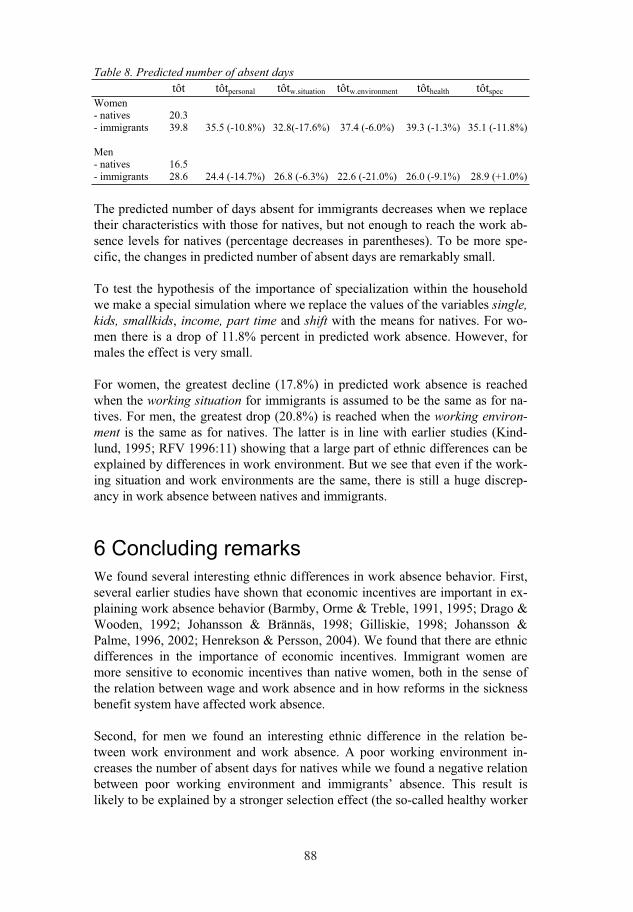
88

Table 8. Predicted number of absent days

tôt tôtpersonal tôtw.situation tôtw.environment tôthealth tôtspec

Women - natives 20.3 - immigrants 39.8 35.5 (-10.8%) 32.8(-17.6%) 37.4 (-6.0%) 39.3 (-1.3%) 35.1 (-11.8%)

Men - natives 16.5 - immigrants 28.6 24.4 (-14.7%) 26.8 (-6.3%) 22.6 (-21.0%) 26.0 (-9.1%) 28.9 (+1.0%)

The predicted number of days absent for immigrants decreases when we replace their characteristics with those for natives, but not enough to reach the work ab-sence levels for natives (percentage decreases in parentheses). To be more spe-cific, the changes in predicted number of absent days are remarkably small.

To test the hypothesis of the importance of specialization within the household we make a special simulation where we replace the values of the variables single,

kids, smallkids, income, part time and shift with the means for natives. For wo-men there is a drop of 11.8% percent in predicted work absence. However, for males the effect is very small.

For women, the greatest decline (17.8%) in predicted work absence is reached when the working situation for immigrants is assumed to be the same as for na-tives. For men, the greatest drop (20.8%) is reached when the working environ-

ment is the same as for natives. The latter is in line with earlier studies (Kind-lund, 1995; RFV 1996:11) showing that a large part of ethnic differences can be explained by differences in work environment. But we see that even if the work-ing situation and work environments are the same, there is still a huge discrep-ancy in work absence between natives and immigrants.

6 Concluding remarks

We found several interesting ethnic differences in work absence behavior. First, several earlier studies have shown that economic incentives are important in ex-plaining work absence behavior (Barmby, Orme & Treble, 1991, 1995; Drago & Wooden, 1992; Johansson & Brännäs, 1998; Gilliskie, 1998; Johansson & Palme, 1996, 2002; Henrekson & Persson, 2004). We found that there are ethnic differences in the importance of economic incentives. Immigrant women are more sensitive to economic incentives than native women, both in the sense of the relation between wage and work absence and in how reforms in the sickness benefit system have affected work absence.

Second, for men we found an interesting ethnic difference in the relation be-tween work environment and work absence. A poor working environment in-creases the number of absent days for natives while we found a negative relation between poor working environment and immigrants’ absence. This result is likely to be explained by a stronger selection effect (the so-called healthy worker

88

89

effect) among immigrant male workers than among natives. In spite of this, we found that if immigrants were to have the same working environment character-istics as natives, i.e. better working environments, their absence would decline. The reform of 1992, when the responsibility for the first two weeks of sick pay was shifted from the public authorities to the employers, was not only motivated by concern over the ill-health index (Prop. 1990/91:181). Moving financial re-sponsibility to the employers was expected to increase incentives for improving work conditions. Thus, if the intensions of the reform were to be fulfilled, we could expect huge gains especially in fields that employ many immigrants.

Third, the way families organize their lives affects natives and immigrants in dif-ferent ways. Having children and working part-time increases work absence for immigrant women but not for native women, which supports our hypothesis of ethnic differences in specialization within the household.

Finally, the major result of our analysis is that the huge gap in number of absent days remains between natives and immigrants work absence even when we give immigrants the same characteristics as natives. Thus we conclude that there are intrinsic differences between natives and immigrants that cannot be explained by the factors considered in this study. At least some of these differences probably have to do with the migration process. There is a vast literature on the problems connected to the reasons for migration, the migration process itself and the cir-cumstances surrounding being an immigrant in a new country (SoS-rapport 1995). These are problems that to some extent can be expected to influence work absence behavior. Including a measure of how many years the immigrant has spent in the new country would be interesting; it might be found that the absence behavior of natives and immigrants converge over the years. Unfortunately we do not have access to data on time since arrival.

To sum up, we wish to stress the need of more research in this area. It would be especially interesting to study the utilization of sickness insurance among unem-ployed immigrants and natives. We have only focused on individuals with jobs, but since the unemployment rate is higher for immigrants, it might be found that immigrants with jobs are more strongly selected than natives with jobs. The dif-ference in utilization of sickness insurance between employed and unemployed might therefore be greater for immigrants than for natives. Another interesting path would be to analyze whether different immigrant groups have different work absence behavior. There is cause to believe that there might be as big varia-tion in absence between different immigrant groups as there is between immi-grants and natives. Unfortunately the sample used in this study is too small to al-low a disaggregated grouping of immigrants.

89

90

ReferencesAkhavan, S & Bildt, C (2004). Arbetsvillkor, hälsa och sjukfrånvaro bland invandrade

kvinnor, Arbetslivsrapport, 2004:21, Arbetslivsinstitutet.

Allen, S G (1981). “An Empirical Model of Work Attendance”. The Review of Economics

and Statistics, vol 63, p 77-87.

Andrén, D (2001). “Work, Sickness, Earnings, and Early Exits from the Labor Market: An

Empirical Analysis Using Swedish Longitudinal Data”. Doctoral Thesis, Department of Economics, Göteborg University,Sweden.

Anxo, D & Flood, L (1997). “Patterns of time use in France and Sweden”, in Persson, I & Jonung, C (eds.), Women’s Work and Wages, London. Routledge

Arai, M & Skogman Thoursie, P (2005). “Incentives and Selection in Cyclical Absentee-ism”. Labour Economics, vol 12 issue 2, p 269-280.

Barmby, T A & Treble, J G (1989). “A Note on Absenteeism”. British Journal of Indus-

trial Relations. vol 27:1, p 155-158.



Becker, G S (1965). “A Theory of the Allocation of Time”. The Economic Journal, vol 75, issue 299, p 493-517.

Björklund, A (1991). “Vem får sjukpenning? En empirisk analys av sjukfrånvarons be-stämningsfaktorer”. I Arbetskraft, arbetsmarknad och produktivitet, Expertrapport nr 4 till Produktivitetsdelegationen.

Bloningen, B A (1997). “Firm-Specific Assets and the Link Between Exchange Rates and Foreign Investment”. The American Economic Review, no 87, vol 3, p 447-465.

Boalt, Å (1989). “Invandrare och hälsa”, i SOU 1989:111.

Brose, P (1995). Sickness absence: an empirical analysis of HUS panel. Working paper 1995:12, Department of Economics, Uppsala University, Uppsala

Bäckman, O (1998). Longitudinal Studies on Sickness Absence in Sweden. Swedish Insti-tute for Social Research, Dissertation Series, no 34.




90

91

Chaudhury, M & Ng, I (1992). “Absenteeism predictors: least squares, rank regression, and model selection results”. Canadian Journal of Economics, no 3, p 615-635.

Dagens Medicin (1999). “Kroppstemperaturen avslöjar patienternas sömnproblem”. 19990601, Stockholm.

Dagens Medicin (2000). “Ökad risk för arbetsskador och hjärtsjukdomar bland nattjobba-re”. 20000516, Stockholm.

Darvishpour, M (1997). “Invandrarkvinnor utmanar männens roll. Maktfördelning och konflikter i iranska familjer” in G. Ahrne & I. Persson (red.) Familj, Makt och jäm-

ställdhet. SOU 1997:138.

Drago, R & Wooden, M (1992). “The determinants of labor absence: Economic factors and work group norms across countries”. Industrial and Labor Relations Review, vol 45, p 764-778.

Dunn, L F & Youngblood S A (1986). “Absenteeism as a Mechanism for Approaching an Optimal Labor Market Equilibrium: An Empirical Study”. The Review of Economics

and Statistics, vol 68, no 4, p 668-674.

Edgerton, D, Kruse, A, & Wells, C (1996). Besparingsåtgärder på socialförsäkringsom-

rådet. En utvärdering av förändringar i sjukpenningförsäkringen. Slutrapport till Riksdagens Revisorer, 1996-09-13, Stockholm.

Ekberg, J (1996). “Invandrarna i pensionssystemet”. Socialvetenskaplig tidskrift, årgång 3, no 4, p 243- 255.

Ekberg, J (1999). “Immigration and the public sector: Income effects for the native popu-lation in Sweden”. Journal of Population Economics, no 12, p 411-430.

Ekberg, J & Andersson, L (1995). Invandring, sysselsättning och ekonomiska effekter. DS 1995:68, Finansdepartementet, Stockholm.

Ekberg, J & Gustavsson, B (1995). Invandrare på arbetsmarknaden. SNS Förlag, Stock-holm.

Ekberg, J & Rooth; D-O (2000). Arbetsmarknadspolitik för invandrare: rapport till riks-

dagens revisorer. Växjö University Working paper Series, no 6. Växjö University, Växjö.

Flood, L & Gråsjö, U (1997). “Tid för barn, tid för arbete. En undersökning av svenska hushålls tidsanvändning”, in Ahrne, G & Persson, I (red), Familj, makt och jämställd-

het, SOU 1997:138.

Franzén, E (1997). “Socialbidrag och invandrare”. Socialvetenskaplig tidskrift, årgång 4, no 4, p 279-394.

Fritzell, J & Lundberg, O (1994). Kvinnor, män och välfärdens utveckling. Institutet för social forskning, Särtryck nr 435, Särtryck ur Har vi råd att avvara välfärden?, För-säkringskasseförbundets FAKTA. Rapport från ett forskarseminarium.

91

92

Gilleskie, D B (1998). “A Dynamic Stochastic Model of Medical Care Use and Work Ab-sence”. Econometrica, vol 66, issue 1, p 1-45.

Greene, W H (2003). Econometric Analysis. Fifth edition. Prentice-Hall International, New Jersey.

Gronau, R (1986). “Home production - A survey” in Ashenfelter, O & Layard, R (eds), Handbook of Labor Economics. vol 1, p 273-304, North Holland, Amsterdam.

Grossman, M (1972). “On the concept of health capital and the demand for health”. Jour-

nal of Political Economy, vol 80, p 223-255.

Gustavsson, B (1986). “Bidragstagarna: Antal och inkomster”. Ds FI 1986:16, Stock-holm.

Gustavsson (1997). “Invandrarnas försörjning” i Mångfald och ursprung – rapport från

ett multietniskt Sverige. Statens Invandrarverk, Norrköping.

Gustavsson, B, Zamanian, M M & Aguilar, R (1990). Invandring och försörjning. Daida-los, Göteborg

Gustavsson, B & Österberg, T (2004). “Ursprung och förtidspension” i Ekberg, J (red) Egenförsörjning eller bidragsförsörjning. Invandrare, arbetsmarknad och välfärdssta-

ten, antologi utgiven av integrationspolitiska maktutredningen, SOU 2004:21.

Hammarstedt, M (2001). Making a living in a new country. Doctoral thesis, Växjö Uni-versity Press, Växjö.

Hansen, J & Löfström, M (2000). “Immigrant assimilation and welfare participation: Do immigrants assimilate into or out-of welfare?”. Journal of Human Resources, vol 38:1, p 74-98.

Hausman, J, Hall, B H & Griliches, Z (1984). “Econometric models for count data with an application to the patents- R&D relationship”. Econometrica, vol 52, no 4, p 909-938.

Henrekson, J, Lantto, K & Persson, M (1992). Bruk och missbruk av sjukförsäkringen.SNS Förlag, Stockholm.



nomics, no 30, p 1493-1503.



92

93

Kindlund, H (1995). “Förtidspensionering och sjukfrånvaro 1990 bland invandrare och svenskar” in Invandrares hälsa och sociala förhållanden. SoS-rapport 1995:5, Social-styrelsen, Stockholm.

Lantto, K & Lindblom, E (1987). “Är arbetslösheten hälsosam?”. Ekonomisk debatt, Nr 4.

Lazear, E P (1999). “Personnel economics: past lessons and future directions: Presidential address to the Society of Labor Economists, San Fransisco, May 1, 1998”. Journal of

Labor Economics, vol 17 (2), p 199-236.


Leinö, T (1983). Invandrarkvinnornas ekonomi och välfärd, in Lundahl, M & Persson, -Tanimura, I (red), Kvinnan i ekonomin, Tillämpad samhällsekonomi, Malmö.

Mathieu, J & Kohler, S (1990). “A Cross-Level Examination of Group Absence Influ-ences on Individual Absence”. Journal of Applied Psychology, vol 75, no 2, p 217-220.

Palme, M & Svensson, I (1998). “Social Security, Occupational Pensions, and Retirement in Sweden”, in Social Security and Retirement Around the World, Gruber, J & Wise, D (eds), Chicago University Press, Chicago.

Paringer, L (1983). “Women and Absenteeism: Health or Economics”. The American

Economic Review, Papers and Proceedings of the Ninety-Fifth Annual Meeting of the American Economic Association, New York, New York, December 29-30, 1982, p 123-27.

Prop 1990/91:181. Regeringens proposition 1990/91:181 om sjuklön, m.m.

RFV (1990). Den med sjukpenning ersatta frånvaron år 1988 efter medborgarskap. Riks-försäkringverket Informerar, Statistisk rapport Is-R 1990:4, Riksförsäkringsverket, Stockholm.



RFV (1996). Invandrare i socialförsäkringen. Sjukskrivning, rehabilitering och förtids-

pensionering under 1990-talet. Riksförsäkringsverket redovisar 1996:11.


Rosen, S (1986). “The theory of equalizing differences” in Ashenfelter, O & Layard, R. (eds) Handbook of Labor Economics, vol 1, p 641-692, North Holland, Amsterdam.

SAF (1986). Tidsanvändningsstatistik, Svenska Arbetgivarföreningen, Stockholm.

Shapiro, C & Stiglitz, J E (1984). “Equilibrium Unemployment as a Worker Discipline Device”. American Economic Review, vol 77, no 3, p 433-444.

93

94

SoS-rapport (1995). Invandrares hälsa och sociala förhållanden. Underlag till Folkhälso-rapport 1994 och Social rapport 1994. SoS-rapport 1995:5, Socialstyrelsen, Stock-holm.

SOU (1979). Kvinnors arbete. En rapport från jämställdhetskommittén. Statens Offentliga Utredningar 1979:89.

SOU (1989). Invandrare i storstad. Underlagsrapport till Storstadsutredningen. Statens Offentliga Utredningar 1989:111.

SOU (2000). Sjukfrånvaro och sjukskrivning – fakta och förslag. Slutbetänkande från Sjukförsäkringsutredningen. Statens Offentliga Utredningar 2000:121.

SOU (2002). En handlingsplan för ökad hälsa i arbetslivet. Slutbetänkande av Utredning-en om handlingsplan för ökad hälsa i arbetslivet. Statens Offentliga Utredningar 2002:5.

SOU (2002). Kunskapsläge sjukförsäkringen. Delbetänkande från Utredningen om analys av hälsa och arbete. Statens Offentliga Utredningar 2002:62.

SOU (2004). Egenförsörjning eller bidragsförsörjning. Invandrarna, arbetsmarknaden

och välfärdsstaten. Ekberg, J (red). Statens Offentliga Utredningar 2004:21


Säll, H (1968). “Våra utlänningar är mer sjuka än vi själva visar statistik i RFV”. Tidskrift

för allmän försäkring, Försäkringskasseförbundet,Stockholm, p 766-772.


Vistnes, J P (1997). “Gender differences in days lost from work due to illness”. Industrial

and Labor Relations Review, vol 50, no 2, p 304-323.

Vogel, J, Hjelm, M & Johansson, SE (2002). Integration till svensk välfärd? :om invand-

rares välfärd på 90-talet. Statistiska centralbyrån, Örebro.

Wells, C et.al. (2004). An analysis of sick leave in Sweden using panel data 1985-1997.

Working paper 2004:3, Department of Economics, Lund University, Lund.

Winkelmann, R (1999). “Wages, firm size and absenteeism”. Applied Economics Letters,vol 6, p 337-341.

Östlin, P et al. (1996). Kön och ohälsa - en antologi om könsskillnader ur ett folkhälso-

perspektiv. Studentlitteratur, Lund.

94

95

Appendix A

Immigrant groups

The immigrants have been divided into the following subgroups :

NordicImmigrants from Norway, Denmark, Finland and Iceland.

Western EuropeImmigrants from Germany, Great Britain, Netherlands, France, Austria, Canada, US and Australia.

Southern EuropeImmigrants from Italy, Greece, Spain, former Yugoslavia and Turkey.

Eastern EuropeImmigrants from Hungary, Poland, former Czechoslovakia, the former Soviet Union and the rest of the European countries.

OthersImmigrants from other countries outside Europe.

95

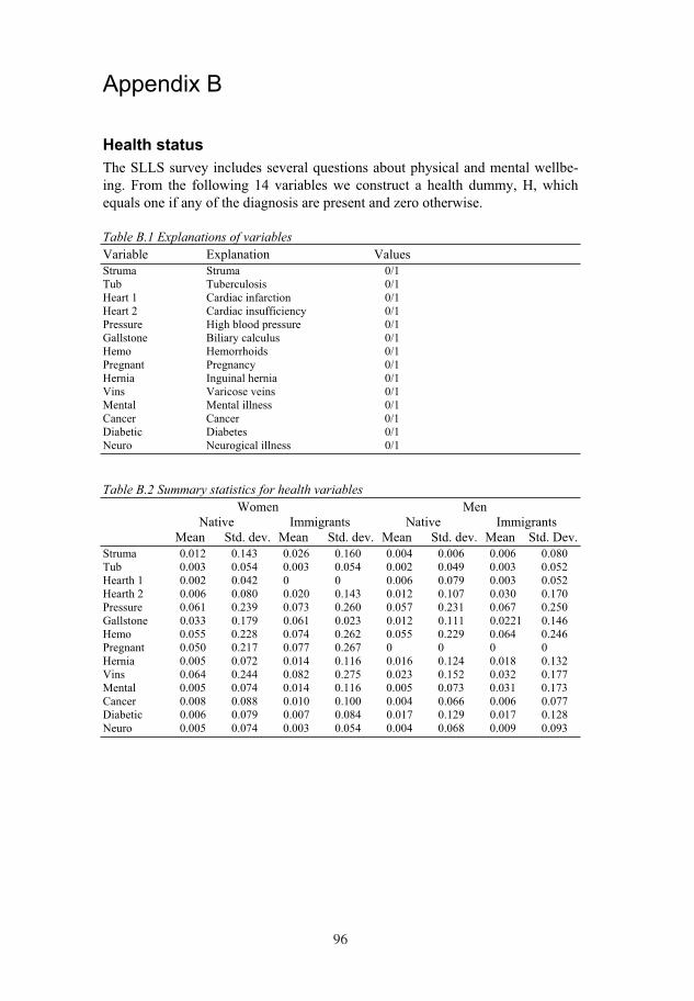
Appendix B

Health status The SLLS survey includes several questions about physical and mental wellbe-ing. From the following 14 variables we construct a health dummy, H, which equals one if any of the diagnosis are present and zero otherwise.

Table B.1 Explanations of variables Variable Explanation Values Struma Struma 0/1 Tub Tuberculosis 0/1 Heart 1 Cardiac infarction 0/1 Heart 2 Cardiac insufficiency 0/1 Pressure High blood pressure 0/1 Gallstone Biliary calculus 0/1 Hemo Hemorrhoids 0/1 Pregnant Pregnancy 0/1 Hernia Inguinal hernia 0/1 Vins Varicose veins 0/1 Mental Mental illness 0/1 Cancer Cancer 0/1 Diabetic Diabetes 0/1 Neuro Neurogical illness 0/1

Table B.2 Summary statistics for health variables Women Men Native Immigrants Native Immigrants Mean Std. dev. Mean Std. dev. Mean Std. dev. Mean Std. Dev. Struma 0.012 0.143 0.026 0.160 0.004 0.006 0.006 0.080 Tub 0.003 0.054 0.003 0.054 0.002 0.049 0.003 0.052 Hearth 1 0.002 0.042 0 0 0.006 0.079 0.003 0.052 Hearth 2 0.006 0.080 0.020 0.143 0.012 0.107 0.030 0.170 Pressure 0.061 0.239 0.073 0.260 0.057 0.231 0.067 0.250 Gallstone 0.033 0.179 0.061 0.023 0.012 0.111 0.0221 0.146 Hemo 0.055 0.228 0.074 0.262 0.055 0.229 0.064 0.246 Pregnant 0.050 0.217 0.077 0.267 0 0 0 0 Hernia 0.005 0.072 0.014 0.116 0.016 0.124 0.018 0.132 Vins 0.064 0.244 0.082 0.275 0.023 0.152 0.032 0.177 Mental 0.005 0.074 0.014 0.116 0.005 0.073 0.031 0.173 Cancer 0.008 0.088 0.010 0.100 0.004 0.066 0.006 0.077 Diabetic 0.006 0.079 0.007 0.084 0.017 0.129 0.017 0.128 Neuro 0.005 0.074 0.003 0.054 0.004 0.068 0.009 0.093

96

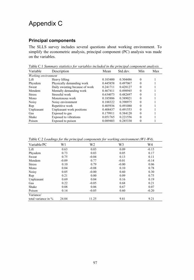
97

Appendix C

Principal components

The SLLS survey includes several questions about working environment. To simplify the econometric analysis, principal component (PC) analysis was made on the variables.

Table C.1 Summary statistics for variables included in the principal component analysis.

Variable Description Mean Std.dev. Min Max Working environment

Lift Heavy lifting 0.103400 0.304486 0 1 Physdem Physically demanding work 0.445858 0.497067 0 1 Sweat Daily sweating because of work 0.241711 0.428127 0 1 Mendem Mentally demanding work 0.467411 0.498945 0 1 Stress Stressful work 0.634073 0.482697 0 1 Mono Monotonous work 0.185886 0.389021 0 1 Noisy Noisy environment 0.188322 0.390975 0 1 Rep Repetitive work 0.405936 0.491080 0 1 Unpleasant Unpleasant work positions 0.408437 0.491553 0 1 Gas Exposed to gas 0.179911 0.384120 0 1 Shake Exposed to vibrations 0.051765 0.221556 0 1 Poison Exposed to poison 0.089403 0.285330 0 1

Table C.2 Loadings for the principal components for working environment (W1-W4).

Variable/PC W1 W2 W3 W4 Lift 0.63 0.03 0.09 -0.15 Physdem 0.73 0.03 0.05 0.17 Sweat 0.75 -0.04 0.13 0.11 Mendem -0.09 0.77 -0.01 -0.14 Stress 0.10 0.79 -0.00 0.06 Mono 0.04 -0.08 0.10 0.78 Noisy 0.05 -0.00 0.60 0.30 Rep 0.21 0.00 0.09 0.75 Unpleasant 0.69 0.04 0.16 0.19 Gas 0.22 -0.05 0.68 0.21 Shake 0.08 0.06 0.67 0.07 Poison 0.14 -0.05 0.60 -0.20

Variance/total variance in % 24.04 11.25 9.81 9.21

97

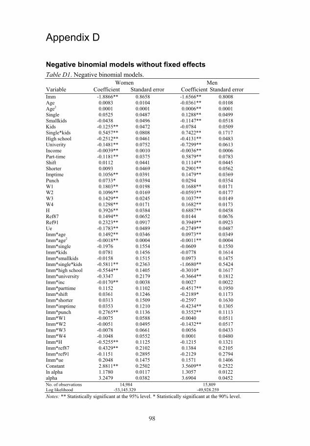
98

Appendix D

Negative binomial models without fixed effects

Table D1. Negative binomial models. Women Men Variable Coefficient Standard error Coefficient Standard error Imm -1.8866** 0.8658 -1.6566** 0.8008 Age 0.0083 0.0104 -0.0361** 0.0108 Age2 0.0001 0.0001 0.0006** 0.0001 Single 0.0525 0.0487 0.1288** 0.0499 Smallkids -0.0438 0.0496 -0.1147** 0.0518 Kids -0.1255** 0.0472 -0.0784 0.0509 Single*kids 0.5457** 0.0808 0.7422** 0.1717 High school -0.2512** 0.0461 -0.4131** 0.0483 Univerity -0.1481** 0.0752 -0.7299** 0.0613 Income -0.0039** 0.0010 -0.0036** 0.0006 Part-time -0.1181** 0.0375 0.5879** 0.0783 Shift 0.0112 0.0441 0.1114** 0.0445 Shorter 0.0093 0.0469 0.2901** 0.0562 Imptime 0.1056** 0.0391 0.1479** 0.0369 Punch 0.0733* 0.0394 0.0294 0.0354 W1 0.1803** 0.0198 0.1688** 0.0171 W2 0.1096** 0.0169 -0.0593** 0.0177 W3 0.1429** 0.0245 0.1037** 0.0149 W4 0.1298** 0.0171 0.1682** 0.0173 H 0.3926** 0.0384 0.6887** 0.0458 Ref87 0.1494** 0.0652 0.0144 0.0676 Ref91 0.2323** 0.0917 0.3949** 0.0923 Ue -0.1783** 0.0489 -0.2749** 0.0487 Imm*age 0.1492** 0.0346 0.0973** 0.0349 Imm*age2 -0.0018** 0.0004 -0.0011** 0.0004 Imm*single -0.1976 0.1554 -0.0609 0.1550 Imm*kids 0.0781 0.1456 -0.0778 0.1614 Imm*smallkids -0.0158 0.1515 0.0973 0.1475 Imm*single*kids -0.5811** 0.2363 -1.0680** 0.5424 Imm*high school -0.5544** 0.1405 -0.3010* 0.1617 Imm*university -0.3347 0.2179 -0.3664** 0.1812 Imm*inc -0.0170** 0.0038 0.0027 0.0022 Imm*parttime 0.1152 0.1102 -0.4517** 0.1950 Imm*shift 0.0361 0.1246 -0.2189* 0.1173 Imm*shorter 0.0313 0.1509 -0.2597 0.1630 Imm*imptime 0.0353 0.1210 -0.4234** 0.1305 Imm*punch 0.2765** 0.1136 0.3552** 0.1113 Imm*W1 -0.0075 0.0588 -0.0040 0.0511 Imm*W2 -0.0051 0.0495 -0.1432** 0.0517 Imm*W3 -0.0078 0.0661 0.0056 0.0433 Imm*W4 -0.1048 0.0552 0.0001 0.0480 Imm*H -0.5255** 0.1125 -0.1215 0.1321 Imm*ref87 0.4329** 0.2102 0.1384 0.2105 Imm*ref91 -0.1151 0.2895 -0.2129 0.2794 Imm*ue 0.2048 0.1475 0.1571 0.1406 Constant 2.8811** 0.2502 3.5609** 0.2522 ln alpha 1.1780 0.0117 1.3057 0.0122 alpha 3.2479 0.0382 3.6904 0.0452 No. of observations 14,984 15,809 Log likelihood -53,145.329 -49,928.259

Notes: ** Statistically significant at the 95% level. * Statistically significant at the 90% level.

98

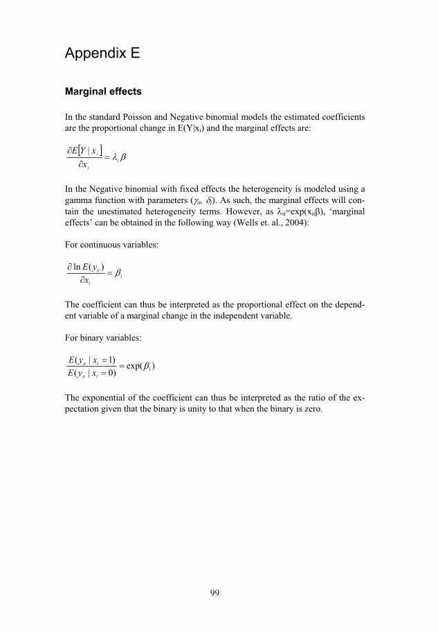
99

Appendix E

Marginal effects

In the standard Poisson and Negative binomial models the estimated coefficients are the proportional change in E(Y|xi) and the marginal effects are:

i

i

i

x

xYE |

In the Negative binomial with fixed effects the heterogeneity is modeled using a gamma function with parameters ( it, i). As such, the marginal effects will con-tain the unestimated heterogeneity terms. However, as it=exp(xit ), ‘marginal effects’ can be obtained in the following way (Wells et. al., 2004):

For continuous variables:

l

l

it

x

yE )(ln

The coefficient can thus be interpreted as the proportional effect on the depend-ent variable of a marginal change in the independent variable.

For binary variables:

)exp()0|(

)1|(l

lit

lit

xyE

xyE

The exponential of the coefficient can thus be interpreted as the ratio of the ex-pectation given that the binary is unity to that when the binary is zero.

99

100100

Acta Wexionensia Nedan följer en lista på skrifter publicerade i den nuvarande Acta-serien, serie III. För förteckning av skrifter i tidigare Acta-serier, se Växjö University Press sidor på www.vxu.se

Serie III (ISSN 1404-4307) 1. Installation Växjö universitet 1999. Nytt universitet – nya professorer. 1999. ISBN 91-7636-233-7

2. Tuija Virtanen & Ibolya Maricic, 2000: Perspectives on Discourse: Proceed-ings from the 1999 Discourse Symposia at Växjö University. ISBN 91-7636-237-X

3. Tommy Book, 2000: Symbolskiften i det politiska landskapet – namn-heraldik-monument. ISBN 91-7636-234-5

4. E. Wåghäll Nivre, E. Johansson & B. Westphal (red.), 2000: Text im Kontext, ISBN 91-7636-241-8

5. Göran Palm & Betty Rohdin, 2000: Att välja med Smålandsposten. Journalis-tik och valrörelser 1982-1998. ISBN 91-7636-249-3

6. Installation Växjö universitet 2000, De nya professorerna och deras föreläs-ningar. 2000. ISBN 91-7636-258-2

7. Thorbjörn Nilsson, 2001: Den lokalpolitiska karriären. En socialpsykologisk studie av tjugo kommunalråd (doktorsavhandling). ISBN 91-7636-279-5

8. Henrik Petersson, 2001: Infinite dimensional holomorphy in the ring of formal power series. Partial differential operators (doktorsavhandling). ISBN 91-7636-282-5

9. Mats Hammarstedt, 2001: Making a living in a new country (doktorsavhan-dling). ISBN 91-7636-283-3

10. Elisabeth Wåghäll Nivre & Olle Larsson, 2001: Aspects of the European Re-formation. Papers from Culture and Society in Reformation Europe, Växjö 26-27 November 1999. ISBN 91-7636-286-8

11. Olof Eriksson, 2001: Aspekter av litterär översättning. Föredrag från ett svensk-franskt översättningssymposium vid Växjö universitet 11-12 maj 2000. ISBN 91-7636-290-6.

12. Per-Olof Andersson, 2001: Den kalejdoskopiska offentligheten. Lokal press, värdemönster och det offentliga samtalets villkor 1880-1910 (Doktorsavhand-ling). ISBN: 91-7636-303-1.

13. Daniel Hjorth, 2001: Rewriting Entrepreneurship. Enterprise discourse and entrepreneurship in the case of re-organising ES (doktorsavhandling). ISBN: 91-7636-304-X.

14. Installation Växjö universitet 2001, De nya professorerna och deras föreläs-ningar, 2001. ISBN 91-7636-305-8.

15. Martin Stigmar, 2002. Metakognition och Internet. Om gymnasieelevers in-formationsanvändning vid arbete med Internet (doktorsavhandling). ISBN 91-7636-312-0.

16. Sune Håkansson, 2002. Räntefördelningen och dess påverkan på skogsbru-ket. ISBN 91-7636-316-3.

17. Magnus Forslund, 2002. Det omöjliggjorda entreprenörskapet. Om förnyel-sekraft och företagsamhet på golvet (doktorsavhandling). ISBN 91-7636-320-1.

18. Peter Aronsson och Bengt Johannisson (red), 2002. Entreprenörskapets dy-namik och lokala förankring. ISBN: 91-7636-323-6.

19. Olof Eriksson, 2002. Stil och översättning. ISBN: 91-7636-324-4

20. Ia Nyström, 2002. ELEVEN och LÄRANDEMILJÖN. En studie av barns lä-rande med fokus på läsning och skrivning (doktorsavhandling). ISBN: 91-7636-351-1

21. Stefan Sellbjer, 2002. Real konstruktivism – ett försök till syntes av två do-minerande perspektiv på undervisning och lärande (doktorsavhandling). ISBN: 91-7636-352-X

22. Harald Säll, 2002. Spiral Grain in Norway Spruce (doktorsavhandling). ISBN: 91-7636-356-2

23. Jean-Georges Plathner, 2003. La variabilité du pronom de la troisième personne en complément prépositionnel pour exprimer le réfléchi (doktorsav-handling). ISBN: 91-7636-361-9

24. Torbjörn Bredenlöw, 2003. Gestaltning – Förändring – Effektivisering. En teori om företagande och modellering. ISBN: 91-7636-364-3

25. Erik Wångmar, 2003. Från sockenkommun till storkommun. En analys av storkommunreformens genomförande 1939-1952 i en nationell och lokal kontext (doktorsavhandling). ISBN: 91-7636-370-8

26. Jan Ekberg (red), 2003, Invandring till Sverige – orsaker och effekter. Års-bok från forskningsprofilen AMER. ISBN: 91-7636-375-9

27. Eva Larsson Ringqvist (utg.), 2003, Ordföljd och informationsstruktur i franska och svenska. ISBN: 91-7636-379-1

28. Gill Croona, 2003, ETIK och UTMANING. Om lärande av bemötande i pro-fessionsutbildning (doktorsavhandling). ISBN: 91-7636-380-5

29. Mikael Askander, 2003, Modernitet och intermedialitet i Erik Asklunds tidiga romankonst (doktorsavhandling). ISBN: 91-7636-381-3

30. Christer Persson, 2003, Hemslöjd och folkökning. En studie av befolknings-utveckling, proto-industri och andra näringar ur ett regionalt perspektiv. ISBN: 91-7636-390-2

31. Hans Dahlqvist, 2003, Fri att konkurrera, skyldig att producera. En ideologi-kritisk granskning av SAF 1902-1948 (doktorsavhandling). ISBN: 91-7636-393-7

32. Gunilla Carlsson, 2003, Det våldsamma mötets fenomenologi – om hot och våld i psykiatrisk vård (doktorsavhandling). ISBN: 91-7636-400-3

33. Imad Alsyouf, 2004. Cost Effective Maintenance for Competitive Advantages (doktorsavhandling). ISBN: 91-7636-401-1.

34. Lars Hansson, 2004. Slakt i takt. Klassformering vid de bondekooperativa slakteriindustrierna i Skåne 1908-1946 (doktorsavhandling). ISBN: 91-7636-402-X.

35. Olof Eriksson, 2004. Strindberg och det franska språket. ISBN: 91-7636-403-8.

36. Staffan Stranne, 2004. Produktion och arbete i den tredje industriella revolu-tionen. Tarkett i Ronneby 1970-2000 (doktorsavhandling). ISBN: 91-7636-404-6.

37. Reet Sjögren, 2004. Att vårda på uppdrag kräver visdom. En studie om vår-dandet av män som sexuellt förgripit sig på barn (doktorsavhandling). ISBN: 91-7636-405-4.

38. Maria Estling Vannestål, 2004. Syntactic variation in English quantified noun phrases with all, whole, both and half (doktorsavhandling). ISBN: 91-7636-406-2.

39. Kenneth Strömberg, 2004. Vi och dom i rörelsen. Skötsamhet som strategi och identitet bland föreningsaktivisterna i Hovmantorp kommun 1884-1930 (doktorsav-handling). ISBN: 91-7686-407-0.

40. Sune G. Dufwa, 2004. Kön, lön och karriär. Sjuksköterskeyrkets omvandling un-der 1900-talet (doktorsavhandling). ISBN: 91-7636-408-9

41. Thomas Biro, 2004. Electromagnetic Wave Modelling on Waveguide Bends, Power Lines and Space Plasmas (doktorsavhandling). ISBN: 91-7636-410-0

42. Magnus Nilsson, 2004, Mångtydigheternas klarhet. Om ironier hos Torgny Lindgren från Skolbagateller till Hummelhonung (doktorsavhandling). ISBN:91-7636-413-5

43. Tom Bryder, 2004. Essays on the Policy Sciences and the Psychology of Po-litics and Propaganda. ISBN: 91-7636-414-3

44. Lars-Göran Aidemark, 2004. Sjukvård i bolagsform. En studie av Helsing-borgs Lasarett AB och Ängelholms Sjukhus AB. ISBN: 91-7636-417-8

45. Per-Anders Svensson, 2004. Dynamical Systems in Local Fields of Charac-teristic Zero (doktorsavhandling). ISBN: 91-7636-418-6

46. Rolf G Larsson, 2004. Prototyping inom ABC och BSc. Erfarenheter från ak-tionsforskning i tre organisationer (doktorsavhandling). ISBN: 91-7636-420-8

47. Päivi Turunen, 2004. Samhällsarbete i Norden. Diskurser och praktiker i omvandling (doktorsavhandling). ISBN: 91-7636-422-4

48. Carina Henriksson, 2004. Living Away from Blessings. School Failure as Lived Experience (doktorsavhandling). ISBN: 91-7636-425-9

49. Anne Haglund, 2004. The EU Presidency and the Northern Dimension Initia-tive: Applying International Regime Theory (doktorsavhandling). ISBN: 91-7636-428-3

50. Ulla Rosén, 2004. Gamla plikter och nya krav. En studie om egendom, kvin-nosyn och äldreomsorg i det svenska agrarsamhället 1815-1939. ISBN: 91-7636-429-1

51. Michael Strand, 2004. Particle Formation and Emission in Moving Grate Bo-ilers Operating on Woody Biofuels (doktorsavhandling). ISBN: 91-7636-430-5

52. Bengt-Åke Gustafsson, 2004. Närmiljö som lärmiljö – betraktelser från Gnosjöregi-onen. ISBN: 91-7636-432-1

53. Lena Fritzén (red), 2004. På väg mot integrativ didaktik. ISBN: 91-7636-433-X

54. M.D. Lyberg, T. Lundström & V. Lindberg, 2004. Physics Education. A short histo-ry. Contemporary interdisciplinary research. Some projects. ISBN: 91-7636-435-6

55. Gunnar Olofsson (red.), 2004. Invandring och integration. Sju uppsatser från forskningsmiljön ”Arbetsmarknad, Migration och Etniska relationer” (AMER) vid Växjö universitet. ISBN: 91-7636-437-2

56. Malin Thor, 2005. Hechaluz – en rörelse i tid och rum. Tysk-judiska ungdo-mars exil i Sverige 1933-1943 (doktorsavhandling). ISBN: 91-7636-438-0

57. Ibolya Maricic, 2005. Face in cyberspace: Facework, (im)politeness and con-flict in English discussion groups (doktorsavhandling). ISBN: 91-7636-444-5

58. Eva Larsson Ringqvist och Ingela Valfridsson (red.), 2005. Forskning om undervisning i främmande språk. Rapport från workshop i Växjö 10-11 juni 2004. ISBN: 91-7636-450-X

59. Vanja Lindberg, 2005. Electronic Structure and Reactivity of Adsorbed Me-tallic Quantum Dots (doktorsavhandling). ISBN: 91-7636-451-8

60. Lena Agevall, 2005. Välfärdens organisering och demokratin – en analys av New Public Management. ISBN: 91-7636-454-2

61. Daniel Sundberg, 2005. Skolreformernas dilemman – En läroplansteoretisk studie av kampen om tid i den svenska obligatoriska skolan (doktorsavhandling). ISBN: 91-7636-456-9.

62. Marcus Nilsson, 2005. Monomial Dynamical Systems in the Field of p-adic Numbers and Their Finite Extensions (doktorsavhandling). ISBN: 91-7636-458-5.

63. Ann Erlandsson, 2005. Det följdriktiga flockbeteendet: en studie om profile-ring på arbetsmarknaden (doktorsavhandling). ISBN: 91-7636-459-3.

64. Birgitta Sundström Wireklint, 2005. Förberedd på att vara oförberedd. En fe-nomenologisk studie av vårdande bedömning och dess lärande i ambulanssjuk-vård (doktorsavhandling). ISBN: 91-7636-460-7

65. Maria Nilsson, 2005. Differences and similarities in work absence behavior – empirical evidence from micro data (doktorsavhandling). ISBN: 91-7636-462-3.

Växjö University Press Växjö universitet 351 95 Växjö www.vxu.se

Differences and similarities in work absence behavior

Documents

Transcript of Differences and similarities in work absence behavior