arX

iv:q

uant

-ph/

0306

028v

1 4

Jun

200

3

Electromagnetic-field quantization and spontaneous decay in left-handed media

Ho Trung Dung,∗ Stefan Yoshi Buhmann, Ludwig Knoll, and Dirk-Gunnar WelschTheoretisch-Physikalisches Institut, Friedrich-Schiller-Universitat Jena, Max-Wien-Platz 1, D-07743 Jena, Germany

Stefan ScheelQuantum Optics and Laser Science, Blackett Laboratory, Imperial College London,

Prince Consort Road, London SW7 2BW, United Kingdom

(Dated: June 4, 2003)

We present a quantization scheme for the electromagnetic field interacting with atomic systemsin the presence of dispersing and absorbing magnetodielectric media, including left-handed materialhaving negative real part of the refractive index. The theory is applied to the spontaneous decayof a two-level atom at the center of a spherical free-space cavity surrounded by magnetodielectricmatter of overlapping band-gap zones. Results for both big and small cavities are presented, andthe problem of local-field corrections within the real-cavity model is addressed.

PACS numbers: 12.20.-m, 42.50.Nn, 42.50.Ct, 78.20.Ci

I. INTRODUCTION

The problem of propagation of electromagnetic wavesin materials having, in a certain frequency range, simul-taneously negative permittivity and permeability thusleading to a negative refractive index was first studiedby Veselago [1]. Since in such materials the electric field,the magnetic field, and wave vector of a plane wave forma left-handed system, so that the direction of the Poynt-ing vector and the wave vector have opposite directions,they are also called left-handed materials (LHMs). Otherunusual properties are a reverse Doppler shift, reverseCerenkov radiation, negative refraction, and reverse lightpressure. Since LHMs do not exist naturally, they haveremained a merely academic curiosity until recent reportson their fabrication [2, 3, 4, 5, 6]. The metamaterials con-sidered there consist of periodic arrays of metallic thinwires to attain negative permittivity, interspersed withsplit-ring resonators to attain negative permeability. Al-though the metamaterials that have been available sofar behave like LHMs only in the microwave range, therehave been suggestions on how to construct metamaterialsthat can operate at optical frequencies, by reducing thesizes of the inclusions (split rings, chiral or omega par-ticles) [7] or by using point defects in photonic crystalsas magnetic emitters [8]. A number of potential appli-cations of LHMs have been proposed, including effectivelight-emitting devices, beam guiders, filters, and near-field lenses. For example, LHMs could be used to real-ize highly efficient low reflectance surfaces [9] or super-lenses which, in principle, can achieve arbitrary subwave-length resolution [10]. The intriguing superlense proposaland the reported observation of negative refraction [3]have touched off intensive and enlightening discussions

∗Also at Institute of Physics, National Center for Sciences and

Technology, 1 Mac Dinh Chi Street, District 1, Ho Chi Minh city,

Vietnam.

[11, 12, 13]. More recent experiments [6] seem to confirmthe negative refraction observed in Ref. [3]. Neverthe-less, there have been still many open questions aboutthe electrodynamics in magnetodielectrics, i.e., materi-als with simultaneously significant electric and magneticproperties, including LHMs.

In this paper, we first study the problem of quanti-zation of the macroscopic electromagnetic field in thepresence of magnetodielectrics, with special emphasis onLHMs. Apart from the more fundamental interest in theproblem, quantization is required to include nonclassicalradiation in the studies. Since dispersion and absorp-tion are related to each other by the Kramers-Kronigrelations, noticeable dispersion implies that absorptionalso cannot be omitted in general. As we will show,quantization of the electromagnetic field in the presenceof dispersing and absorbing magnetodielectrics can beperformed by means of a source-quantity representationbased on the classical Green tensor in a similar way as inRefs. [14, 15, 16, 17, 18, 19] for purely dielectric material.

As a simple application of the quantization scheme, wethen study the spontaneous decay of an excited two-levelatom in a dispersing and absorbing magnetodielectric en-vironment, with special emphasis on an atom in a spher-ical cavity. It is well-known that the spontaneous decayof an atom is influenced by the environment. If the atomis embedded in a homogeneous, purely electric mediumwith real and positive (frequency-independent) permit-tivity, the decay rate without local-field corrections reads

Γ = nΓ0, (1)

where Γ0 is the decay rate in free space and n=√ε is the

refractive index (see, e.g., [20, 21] and references therein).From energy scaling arguments it can be inferred that theelectric field in a medium corresponds to the electric fieldin free space times 1/

√ε. From a mode decomposition

one can conclude that the mode density is proportional ton3. With that, Eq. (1) immediately follows from Fermi’sgolden rule. Now if we take into account that in the

2

more general case of positive ε and µ the refractive indexis n=

√εµ, we conclude that

Γ = µnΓ0. (2)

Unfortunately, these arguments cannot be used if, e.g.,µ and n are simultaneously negative. Basing the calcu-lations on rigorous quantization, we show that Eq. (2)also remains valid in this case. Moreover, we generalizeEq. (2) to the realistic case of dispersing and absorbingmatter, including local-field effects.

The article is organized as follows. In Sec. II, some gen-eral aspects of the refractive index of a medium whosepermittivity and permeability can simultaneously be-come negative are discussed. Section III is devoted to thequantization of the electromagnetic field in the presenceof a dispersing and absorbing magnetodielectric medium.The interaction of the medium-assisted field with addi-tional charged particles is considered in Sec. IV and theminimal-coupling Hamiltonian is given. In Sec. V, thetheory is applied to the spontaneous decay of an excitedtwo-level atom, with special emphasis on an atom in aspherical cavity surrounded by a dispersing and absorb-ing magnetodielectric. A summary and some concludingremarks are given in Sec. VI.

II. PERMITTIVITY, PERMEABILITY, AND

REFRACTIVE INDEX

Let us consider a causal linear magnetodielectric me-dium characterized by a (relative) permittivity ε(r, ω)and a (relative) permeability µ(r, ω), both of which arespatially varying, complex functions of frequency satisfy-ing the relations

ε(r,−ω∗) = ε∗(r, ω), µ(r,−ω∗) = µ∗(r, ω). (3)

They are holomorphic in the upper complex half-planewithout zeros and approach unity as the frequency goesto infinity,

lim|ω|→∞

ε(r, ω) = lim|ω|→∞

µ(r, ω) = 1. (4)

Since for absorbing media Im ε(r, ω) > 0, Imµ(r, ω) > 0(see, e.g., Ref. [22]), we may write

ε(r, ω) = |ε(r, ω)|eiφε(r,ω), φε(r, ω) ∈ (0, π), (5)

µ(r, ω) = |µ(r, ω)|eiφµ(r,ω), φµ(r, ω) ∈ (0, π). (6)

The relation n2(r, ω) = ε(r, ω)µ(r, ω) formally offers twopossibilities for the (complex) refractive index n(r, ω),

n(r, ω) = ±√

|ε(r, ω)µ(r, ω)| ei[φε(r,ω)+φµ(r,ω)]/2, (7)

where

0 < [φε(r, ω) + φµ(r, ω)]/2 < π. (8)

The ± sign in Eq. (7) leads to Imn(r, ω)≷ 0. To specifythe sign, different arguments can be used. From the high-frequency limit of the permittivity and the permeability,Eq. (4), and the requirement that lim|ω|→∞ n(r, ω)=1 itfollows that the + sign is correct [12],

n(r, ω) =√

|ε(r, ω)µ(r, ω)| ei[φε(r,ω)+φµ(r,ω)]/2. (9)

The same result can be found from energy arguments [9][see also the remark following Eq. (27) in Sec. III andSec. V A].

From Eq. (9) it can be seen that when both ε(r, ω)and µ(r, ω) have negative real parts [φε(r, ω), φµ(r, ω) ∈(π/2, π)], then Ren(r, ω) is also negative. It should bepointed out that for negative Ren(r, ω) it is not nec-essary that Re ε(r, ω) and Reµ(r, ω) are simultaneouslynegative. For the real part of the refractive index tobe negative, it is sufficient that [φε(r, ω) + φµ(r, ω)] >π, i.e., one of the phases can still be smaller than π/2,provided the other one is large enough. In fact, the def-inition of LHMs was originally introduced for frequencyranges where material absorption is negligible small, andthus ε(r, ω) and µ(r, ω) can be regarded as being real[1]. In this case propagating waves can exist providedthat both ε(r, ω) and µ(r, ω) are simultaneously eitherpositive or negative. If they have different signs, thenthe refractive index is purely imaginary, and only evanes-cent waves are supported. The situation becomes morecomplicated when material absorption cannot be disre-garded, because there is always a nonvanishing real partof the refractive index (apart from the specific case where[φε(r, ω) + φµ(r, ω)] = π). In the following we refer to amaterial as being left-handed if the real part of its refrac-tive index is negative.

In order to illustrate the dependence on frequency ofthe refractive index, let us restrict our attention to asingle-resonance permittivity

ε(ω) = 1 +ω2

Pe

ω2Te − ω2 − iωγe

(10)

and a single-resonance permeability

µ(ω) = 1 +ω2

Pm

ω2Tm − ω2 − iωγm

, (11)

where ωPe, ωPm are the coupling strengths, ωTe, ωTm

are the transverse resonance frequencies, and γe, γm arethe absorption parameters. For notational convenience,we have omitted the spatial argument. Both the permit-tivity and the permeability satisfy the Kramers-Kronigrelations. Equation (10) corresponds to the well-known(single-resonance) Drude-Lorentz model of the permittiv-ity. The permeability given by Eq. (11), which is of thesame type as Eq. (10), can be derived by using a damped-harmonic oscillator model for the magnetization [23]. Italso occurs in the magnetic metamaterials constructedrecently [2, 3, 6, 24].

For very small material absorption (γe/m ≪ ωPe/m,ωTe/m), the permittivity (10) and the permeability (11),

3

-20

0

20

40

0.95 1 1.05 1.1

-4

0

4

1.01 1.03 1.05

0

20

40

0.95 1 1.05 1.1

(a)

(b)

ω/ω

nn

ImR

e

Tm

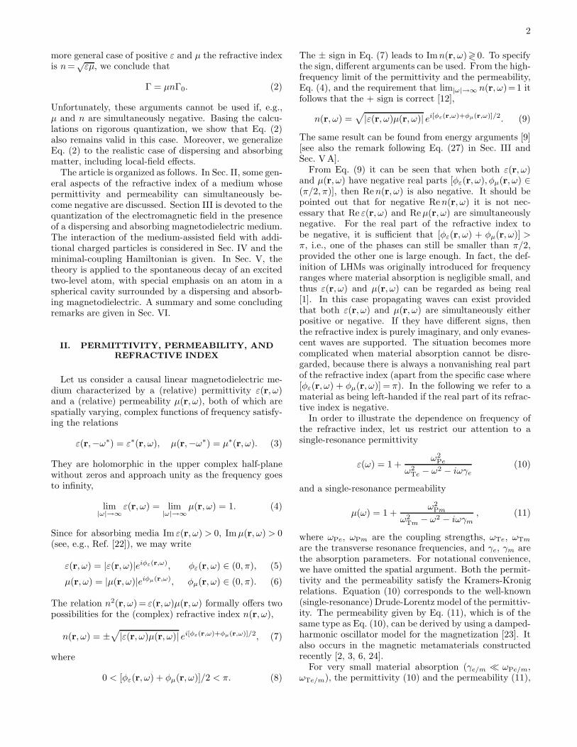
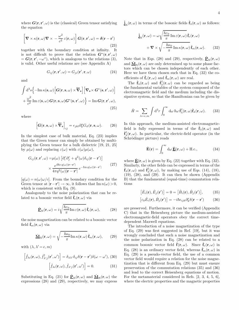
FIG. 1: Real (a) and imaginary (b) parts of the refractiveindex n(ω) as functions of frequency, with the permittivityε(ω) and the permeability µ(ω) being respectively given byEqs. (10) and (11) [ωTe = 1.03 ωTm; ωPm = 0.43 ωTm; ωPe =0.75 ωTm; γe =γm = 0.001 ωTm (solid lines), 0.01 ωTm (dashedlines), and 0.05 ωTm (dotted lines)]. The values of the param-eters have been chosen to be similar to those in Refs. [3, 13].

respectively, feature band gaps between the transversefrequency ωTe and the longitudinal frequency ωLe =√

ω2Te + ω2

Pe, where Re ε(ω)< 0, and the transverse fre-quency ωTm and the longitudinal frequency ωLm =√

ω2Tm + ω2

Pm, where Reµ(ω)< 0. With increasing val-ues of γe and γm the band gaps are shifted to higherfrequencies and smoothed out. Figure 1 shows the de-pendence on frequency of the refractive index [Eq. (9)]for the case of overlapping band gaps and various ab-sorption parameters. In particular, if max (ωTe, ωTm)<ω < min (ωLe, ωLm), then Re ε(ω) < 0 and Reµ(ω)< 0,and thus a negative real part of the refractive index isobserved. In Fig. 1, this is the case in the frequencyinterval where 1.03 < ω/ωTm < 1.088. For the chosenparameters, a negative real part of the refractive indexcan also be realized for frequencies slightly smaller thanωTe, where Reµ(ω) < 0 while Re ε(ω) > 0, as is clearlyseen from the inset in Fig. 1(a). In this region, how-ever, |Ren(ω)| is typically small whereas Imn(ω) is largethereby effectively inhibiting traveling waves. It is worth

noting that a negative real part of the refractive indexis typically observed together with strong dispersion, sothat absorption cannot be disregarded in general. On theother hand, increasing absorption smooths the frequencyresponse of the refractive index thereby making negativevalues of the refractive index less pronounced.

III. THE QUANTIZED MEDIUM-ASSISTED

ELECTROMAGNETIC FIELD

The quantization of the electromagnetic field in acausal linear magnetodielectric medium characterized byboth ε(r, ω) and µ(r, ω) can be performed by generaliz-ing the theory given in Refs. [16, 19] for dielectric media.

Let P(r, ω) and M(r, ω), respectively, be the operatorsof the polarization and the magnetization in frequencyspace. The operator-valued Maxwell equations in fre-quency space then read

∇B(r, ω) = 0, (12)

∇D(r, ω) = 0, (13)

∇× E(r, ω) = iωB(r, ω), (14)

∇× H(r, ω) = −iωD(r, ω), (15)

where

D(r, ω) = ε0E(r, ω) + P(r, ω), (16)

H(r, ω) = κ0B(r, ω)− M(r, ω) (17)

[κ0 = µ−10 ]. Similarly to the electric constitutive relation,

P(r, ω) = ε0[ε(r, ω)− 1]E(r, ω) + PN(r, ω), (18)

with PN(r, ω) being the noise polarization associatedwith the electric losses due to material absorption, weintroduce the magnetic constitutive relation

M(r, ω) = κ0[1− κ(r, ω)]B(r, ω) + MN(r, ω), (19)

where κ(r, ω)=µ−1(r, ω), and MN(r, ω) is the noise mag-netization unavoidably associated with magnetic losses.Recall that for absorbing media Imµ(r, ω)> 0, and thusImκ(r, ω)< 0. Substituting Eqs. (14) and (16)–(19) intoEq. (15), we obtain

∇×κ(r, ω)∇×E(r, ω)−ω2

c2ε(r, ω)E(r, ω) = iωµ0jN(r, ω),

(20)where

jN(r, ω) = −iωPN(r, ω) + ∇× MN(r, ω) (21)

is the noise current. The noise charge density is givenby ρ

N(r, ω) =−∇PN(r, ω), and the continuity equation

holds. The solution of Eq. (20) can be given by

E(r, ω) = iωµ0

∫

d3r′ G(r, r′, ω) jN(r′, ω), (22)

4

where G(r, r′, ω) is the (classical) Green tensor satisfyingthe equation

[

∇× κ(r, ω)∇× − ω2

c2ε(r, ω)

]

G(r, r′, ω) = δ(r − r′)

(23)together with the boundary condition at infinity. Itis not difficult to prove that the relation G∗(r, r′, ω)= G(r, r′,−ω∗), which is analogous to the relations (3),is valid. Other useful relations are (see Appendix A)

Gij(r, r′, ω) = Gji(r

′, r, ω) (24)

and∫

d3s{

−Imκ(s, ω)[

G(r, s, ω)×←−∇s

][

∇s×G∗(s, r′, ω)

]

+ω2

c2Im ε(s, ω)G(r, s, ω)G∗(s, r′, ω)

}

= Im G(r, r′, ω),

(25)

where[

G(r, s, ω)×←−∇s

]

ij= ǫjkl∂

skGil(r, s, ω). (26)

In the simplest case of bulk material, Eq. (23) impliesthat the Green tensor can simply be obtained by multi-plying the Green tensor for a bulk dielectric [19, 21, 25]by µ(ω) and replacing ε(ω) with ε(ω)µ(ω),

Gij(r, r′, ω) =µ(ω)

[

∂ri ∂

rj + q2(ω)δij(r− r′)

]

× eiRe q(ω)|r−r′|

4πq2(ω)|r− r′| e−Im q(ω)|r−r

′|(27)

[q(ω) = n(ω)ω/c]. From the boundary condition for theGreen tensor at |r−r′| → ∞, it follows that Imn(ω)> 0,which is consistent with Eq. (9).

Analogously to the noise polarization that can be re-

lated to a bosonic vector field fe(r, ω) via

PN(r, ω) = i

√

~ε0π

Im ε(r, ω) fe(r, ω), (28)

the noise magnetization can be related to a bosonic vector

field fm(r, ω) via

MN(r, ω) =

√

−~κ0

πImκ(r, ω) fm(r, ω), (29)

with (λ, λ′ = e,m)

[

fλi(r, ω), f †λ′j(r

′, ω′)]

= δλλ′δijδ(r− r′)δ(ω − ω′), (30)

[

fλi(r, ω), fλ′j(r′, ω′)

]

= 0. (31)

Substituting in Eq. (21) for PN(r, ω) and MN(r, ω) theexpressions (28) and (29), respectively, we may express

jN(r, ω) in terms of the bosonic fields fλ(r, ω) as follows:

jN(r, ω) = ω

√

~ε0π

Im ε(r, ω) fe(r, ω)

+ ∇×√

−~κ0

πImκ(r, ω) fm(r, ω). (32)

Note that in Eqs. (28) and (29), respectively, PN(r, ω)

and MN(r, ω) are only determined up to some phase fac-tors which can be chosen independently of each other.Here we have them chosen such that in Eq. (32) the co-

efficients of fe(r, ω) and fm(r, ω) are real.

The fλ(r, ω) and f†λ(r, ω) can be regarded as being

the fundamental variables of the system composed of theelectromagnetic field and the medium including the dis-sipative system, so that the Hamiltonian can be given by

H =∑

λ=e,m

∫

d3r

∫ ∞

0

dω ~ω f†λ(r, ω)fλ(r, ω). (33)

In this approach, the medium-assisted electromagnetic-

field is fully expressed in terms of the fλ(r, ω) and

f†λ(r, ω). In particular, the electric-field operator (in the

Schrodinger picture) reads

E(r) =

∫ ∞

0

dω E(r, ω) + H.c., (34)

where E(r, ω) is given by Eq. (22) together with Eq. (32).Similarly, the other fields can be expressed in terms of the

fλ(r, ω) and f†λ(r, ω), by making use of Eqs. (14), (18),

(19), (28), and (29). It can then be shown (AppendixB) that the fundamental (equal-time) commutation rela-tions

[

Ei(r), Ej(r′)]

= 0 =[

Bi(r), Bj(r′)

]

, (35)[

ε0Ei(r), Bj(r′)

]

= −i~ǫijk∂rkδ(r − r′) (36)

are preserved. Furthermore, it can be verified (AppendixC) that in the Heisenberg picture the medium-assistedelectromagnetic-field operators obey the correct time-dependent Maxwell equations.

The introduction of a noise magnetization of the typeof Eq. (29) was first suggested in Ref. [19], but it waswrongly concluded that such a noise magnetization andthe noise polarization in Eq. (28) can be related to a

common bosonic vector field f (r, ω). Since fe(r, ω) in

Eq. (28) is an ordinary vector field, whereas fm(r, ω) inEq. (29) is a pseudo-vector field, the use of a commonvector field would require a relation for the noise magne-tization that is different from Eq. (29) but must ensurepreservation of the commutation relations (35) and (36)and lead to the correct Heisenberg equations of motion.For the metamaterial considered in Refs. [2, 3, 4, 5, 6],where the electric properties and the magnetic properties

5

are provided by physically different material components,the assumption that the polarization and the magnetiza-tion are related to different basic variables is justified. Itis also in the spirit of Ref. [23], where the polarizationand the magnetization are caused by different degrees offreedom.

IV. INTERACTION OF THE

MEDIUM-ASSISTED FIELD WITH CHARGED

PARTICLES

In order to study the interaction of charged particleswith the medium-assisted electromagnetic field, we firstintroduce the scalar potential

ϕ(r) =

∫

dω ϕ(r, ω) + H.c. (37)

and the vector potential

A(r) =

∫

dω A(r, ω) + H.c., (38)

where in the Coulomb gauge, ϕ(r, ω) and A(r, ω) are

respectively related to the longitudinal part E‖(r, ω) and

the transverse part E⊥(r, ω) of E(r, ω) [Eq. (22) togetherwith Eq. (32)] according to

−∇ϕ(r, ω) = E‖(r, ω), (39)

A(r, ω) = (iω)−1E⊥(r, ω). (40)

Similarly, the momentum field Π(r) that is canonically

conjugated with respect to the vector potential A(r) can

be constructed noting that Π(r, ω) =−ε0E⊥(r, ω). Nowthe Hamiltonian (33) can be supplemented by terms de-scribing the energy of the charged particles and their in-teraction energy with the medium-assisted electromag-netic field in the same way as in Ref. [19] for dielectricmatter. In the minimal-coupling scheme and for non-relativistic particles, the total Hamiltonian then reads

H =∑

λ=e,m

∫

d3r

∫ ∞

0

dω ~ω f†λ(r, ω)fλ(r, ω)

+∑

α

1

2mα

[

pα − qαA(rα)]2

+ 12

∫

d3rρA(r)ϕA(r) +

∫

d3rρA(r)ϕ(r), (41)

where rα, and pα are respectively the position and thecanonical momentum operator of the αth particle of massmα and charge qα. The first term in Eq. (41) is theHamiltonian (33) of the electromagnetic field and themedium including the dissipative system. The secondterm is the kinetic energy of the charged particles, and

the third term is their Coulomb energy, with

ρA(r) =∑

α

qαδ(r− rα), (42)

ϕA(r) =

∫

d3r′ρA(r′)

4πε0|r− r′| (43)

being respectively the charge density and the scalar po-tential of the particles. Finally, the last term is theCoulomb energy of the interaction between the chargedparticles and the medium.

Let ~E(r) and ~B(r) be respectively the operators of theelectric field and the induction field in the presence of thecharged particles

~E(r) = E(r) −∇ϕA(r), ~B(r) = B(r). (44)

Accordingly, the displacement field ~D(r) and the mag-

netic field ~H(r) in the presence of the charged particlesare given by

~D(r) = D(r) − ε0∇ϕA(r), ~H(r) = H(r). (45)

Note that in Eqs. (44) and (45) the electromagnetic fieldsmust be thought of as being expressed in terms of the fun-

damental fields fλ(r) and f†λ(r). From the construction

of the induction field and the displacement field it followsthat they obey the time-independent Maxwell equations

∇ ~B(r) = 0, ∇ ~D(r) = ρA(r). (46)

Further, it can be shown (Appendix C) that the Hamil-tonian (41) generates the correct Heisenberg equations ofmotion, i.e., the time-dependent Maxwell equations

∇× ~E(r) +˙~B(r) = 0, (47)

∇× ~H(r) −˙~D(r) = jA(r), (48)

where

jA(r) = 12

∑

α

qα

[

˙rαδ(r− rα) + δ(r− rα) ˙rα

]

, (49)

and the Newtonian equations of motion for the chargedparticles

˙rα =1

mα

[

pα − qαA(rα)]

, (50)

mα¨rα = qα

{

~E(rα) + 12

[

˙rα × ~B(rα)− ~B(rα)× ˙rα

]}

.

(51)

6

V. SPONTANEOUS DECAY OF AN EXCITED

TWO-LEVEL ATOM

Let us consider a two-level atom (position rA, tran-sition frequency ωA) that resonantly interacts withthe electromagnetic field in the presence of magnetodi-electrics and restrict our attention to the electric-dipoleand the rotating-wave approximations. By analogy withthe case of an atom in the presence of dielectric material[19, 26], the Hamiltonian (41) reduces to

H =∑

λ=e,m

∫

d3r

∫ ∞

0

dω ~ω f†λ(r, ω)fλ(r, ω)

+ ~ωAσ†σ −

[

σ†dA

∫ ∞

0

dω E(rA, ω) + H.c.

]

, (52)

where σ = |l〉〈u| and σ† = |u〉〈l| are the Pauli operatorsof the two-level atom. Here, |l〉 is the lower state whoseenergy is set equal to zero and |u〉 is the upper state

of energy ~ωA. Further, dA = 〈l|dA|u〉= 〈u|dA|l〉 is thetransition dipole moment.

To study the spontaneous decay of an initially excitedatom, we may look for the system wave function at time

t in the form of [|1λ(r, ω)〉≡ f†λ(r, ω)|{0}〉]

|ψ(t)〉 = Cu(t)e−iωAt|{0}〉|u〉

+∑

λ=e,m

∫

d3r

∫ ∞

0

dω e−iωtCλl(r, ω, t)|1λ(r, ω)〉|l〉, (53)

where Cu(t) and Cλl(t) are slowly varying amplitudesand, in anticipation of the environment-induced tran-sition frequency shift δω [27], ωA = ωA − δω is theshifted transition frequency. The Schrodinger equationi~∂t|ψ(t)〉= H |ψ(t)〉 then leads to the set of differentialequations

Cu(t) = −iδωCu(t)− 1√πε0~

∫ ∞

0

dωω

ce−i(ω−ωA)t

×∫

d3rdA

{

ω

c

√

Im ε(r, ω)G(rA, r, ω)Cel(r, ω, t)

+√

−Imκ(r, ω)[

G(rA, r, ω)×←−∇r

]

Cml(r, ω, t)

}

, (54)

Cel(r, ω, t) =1√πε0~

ω2

c2

√

Im ε(r, ω) ei(ω−ωA)t

×dAG∗(rA, r, ω)Cu(t), (55)

Cml(r, ω, t) =1√πε0~

ω

c

√

−Imκ(r, ω) ei(ω−ωA)t

×dA

[

G∗(rA, r, ω)×←−∇r

]

Cu(t), (56)

which has to be solved under the initial conditions Cu(0)=1, Cλl(r, ω, 0)=0. Formal integrations of Eqs. (55) and

(56) and substitution into Eq. (54) leads to, upon usingthe relation (25),

Cu(t) = −iδωCu(t) +

∫ t

0

dt′K(t− t′)Cu(t′), (57)

where

K(t− t′) = − 1

~πε0

∫ ∞

0

dωω2

c2

× e−i(ω−ωA)(t−t′)dAIm G(rA, rA, ω)dA. (58)

It should be noted that, by integrating with respect to t,the integro-differential equation (57) can equivalently beexpressed in the form of a Volterra integral equation ofsecond kind [26]. Equations (57) and (58) formally looklike those valid for non-magnetic structures [26]. Sincethe matter properties are fully included in the Green ten-sor, the results only differ in the actual Green tensor.

Equations (57) and (58) apply to an arbitrary cou-pling regime [26]. Here, we restrict our attention to theweak-coupling regime, where the Markov approximationapplies. That is to say, we may replace Cu(t′) in Eq. (57)by Cu(t) and approximate the time integral according to

∫ t

0

dt′e−i(ω−ωA)(t−t′) → ζ(ωA − ω) (59)

[ζ(x) = πδ(x) + iP/x]. Identifying the principal-part in-tegral with the transition-frequency shift, we obtain

δω =1

π~ε0P

∫ ∞

0

dωω2

c2dAIm G(rA, rA, ω)dA

ω − ωA, (60)

which, together with Eq. (53), can be regarded as beingthe self-consistent defining equation for the transition-frequency shift [27]. Equation (57) then yields Cu(t) =exp(− 1

2Γt), where the decay rate Γ is given by the formula

Γ =2ω2

A

~ε0c2dAIm G(rA, rA, ωA)dA, (61)

which is obviously valid independently of the (material)surroundings of the atom.

A. Nonabsorbing bulk material

Let us first consider the limiting case of non-absorbingbulk material, i.e., ε(ωA) and µ(ωA) are assumed to bereal. Using the bulk-material Green tensor (27), it caneasily be proved that

Im G(rA, rA, ωA)=ωA

6πcRe [µ(ωA)n(ωA)] I. (62)

Substitution into Eq. (61) yields the decay rate

Γ = Re [µ(ωA)n(ωA)] Γ0, (63)

7

where

Γ0 =ω3

Ad2A

3~πε0c3(64)

is the free-space decay rate, but taken at the shifted tran-sition frequency. Eq. (63) is in agreement with Eq. (2) ob-tained from simple arguments on the change of the energydensity and the mode density for positive and frequency-independent ε and µ. Clearly, Eq. (63) is more general inthat it also applies to dispersive magnetodielectrics. Inparticular, when ε(ωA) and µ(ωA) have opposite signs,then the refractive index defined according to Eq. (9)is purely imaginary, thereby leading to Γ =0. This isbecause the electromagnetic field cannot be excited atωA, so that spontaneous emission is completely inhib-ited. Note that material absorption always gives rise toa finite value of Γ, which of course can be very small.

From Eq. (63) it is clearly seen that for non-absorbingLHM, i.e., ε(ωA)< 0 and µ(ωA)< 0, the now real refrac-tive index must also be negative, in order to arrive at anon-negative value of the decay rate. This is yet anotherstrong argument for the choice of the + sign in Eq. (7).

B. Atom in a spherical cavity

For realistic bulk material, the imaginary part of theGreen tensor at equal positions is singular [19, 21, 25].Physically, this singularity is fictitious, because the atom,though surrounded by matter, is always localized in asmall free-space region. The Green tensor for such aninhomogeneous system reads

G(r, r′, ω) = GV(r, r′, ω) + G

S(r, r′, ω), (65)

where GV(r, r′, ω) is the vacuum Green tensor and

GS(r, r′, ω) is the scattering part, which describes theeffect of reflections at the surface of discontinuity. UsingEq. (65) together with ImGV(r, r, ω) = (ω/6πc)I [cf.Eq. (62)], we can write the decay rate (61) as

Γ = Γ0 +2ω2

A

~ε0c2dAIm G

S(rA, rA, ωA)dA, (66)

which is again seen to be valid for any type of material.Within a ‘classical’ theory of spontaneous emission

[28], a formula of the type (66) has been used in Ref. [29]

to calculate the decay rate of an atom near a dispersion-less and absorptionless LHM sphere. ‘Classical’ theorymeans here, that a classically moving dipole in the pres-ence of macroscopic bodies is considered, with the valueof Γ0 being borrowed from quantum mechanics. As inRef. [29], the atomic transition frequency is commonlyunderstood as being that in free space. From Eq. (66) itis seen that the medium-assisted (i.e., shifted) frequencyωA must be used instead of the free-space frequency ωA,since both values can differ substantially.

Let us apply Eq. (66) to an atom in a free-space re-gion surrounded by a multilayer sphere. Using the Greentensor given in Ref. [30], we obtain

Γ⊥

Γ0= 1 + 3

2

∞∑

n=1

n(n+ 1)(2n+ 1)

[

jn(kArA)

kArA

]2

ReCNn

(67)for a radially oriented dipole moment (dA ‖ rA) and

Γ‖

Γ0= 1 + 3

4

∞∑

n=1

(2n+ 1)

[

j2n(kArA)ReCMn

+

(

[kArAjn(kArA)]′

kArA

)2

ReCNn

]

(68)

for a tangentially oriented dipole moment (dA⊥ rA) [theprime indicating the derivative with respect to kArA,

(kA = ωA/c)]. In Eqs. (67) and (68), jn(z) and h(1)n (z)

are the spherical Bessel and Hankel functions of the firstkind, respectively. The coefficients CN

n and CMn have to

be determined through recurrence formulas [30].

Equations (67) and (68) apply to an atom at an ar-bitrary position inside a spherical free-space cavity sur-rounded by an arbitrary spherical multilayer material en-vironment. Let us specify the system such that the atomis situated at the center of the cavity (i.e., rA = 0) andlet the surrounding material homogeneously extend overall the remaining space. For small cavity radii, the sys-tem corresponds to the real-cavity model of local-fieldcorrections. Making use of the explicit expressions forthe coefficients CN

n as in Ref. [30] and the fact that forrA = 0 only the n= 1 term in Eq. (67) contributes [31],we derive from Eq. (67)

Γ

Γ0= 1 + Re

[

1− i(n+ 1)z − n(n+ 1)µ−nµ−n2

z2 + in2 µ−nµ−n2

z3

]

eiz

−i sin z − (n sin z − i cos z)z +

(

cos z − i 1−µµ−n2

n sin z

)

nz2 − (n sin z + iµ cos z)n2

µ−n2z3

(69)

[µ=µ(ωA), n=n(ωA), and z=RωA/c, with R being the cavity radius]. Obviously, the dipole orientation does not

8

0.01

1

100

1 1.1 1.2 1.3

0.01

1

100

1 1.1 1.2 1.3

0.01

1

100

1 1.1 1.2 1.3

(a)

(b)

(c)

ω /ω

Γ/Γ

Γ/Γ

Γ/Γ

00

0

A~

mT

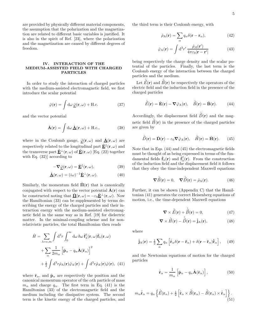
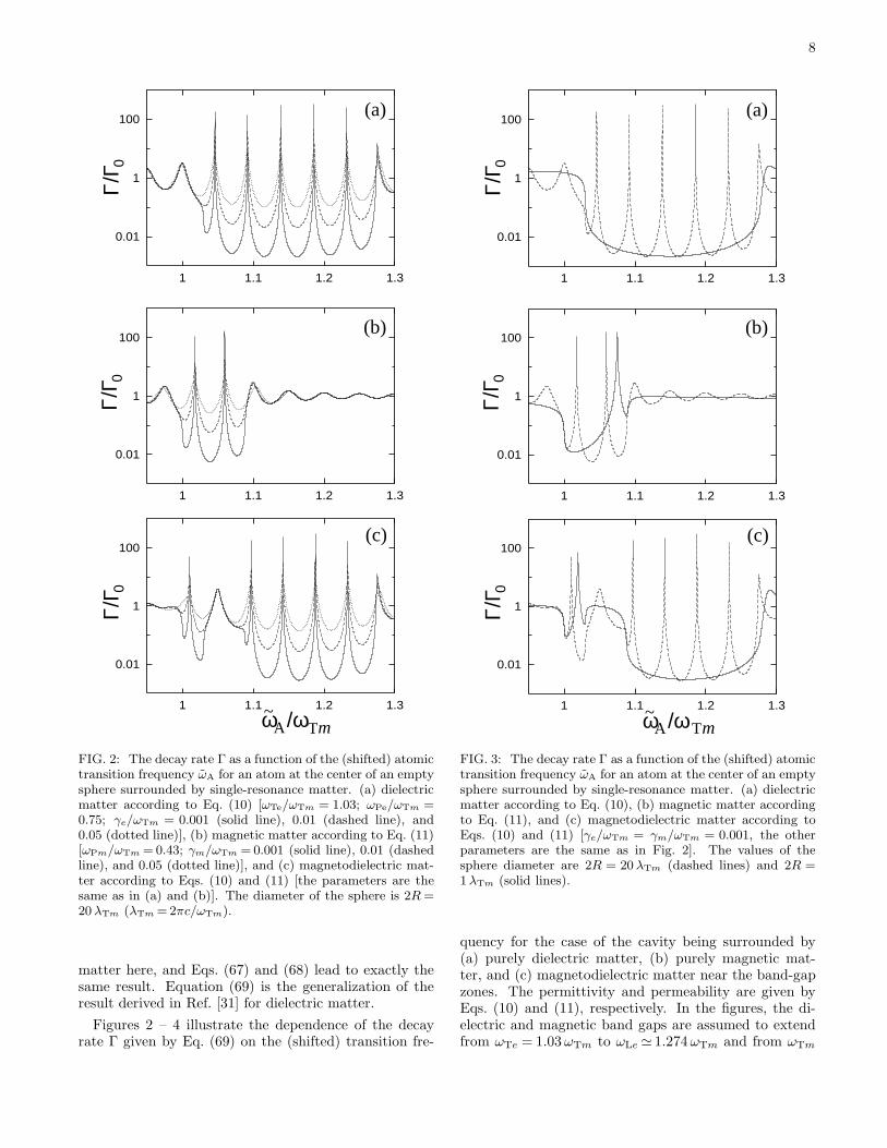
FIG. 2: The decay rate Γ as a function of the (shifted) atomictransition frequency ωA for an atom at the center of an emptysphere surrounded by single-resonance matter. (a) dielectricmatter according to Eq. (10) [ωTe/ωTm = 1.03; ωPe/ωTm =0.75; γe/ωTm = 0.001 (solid line), 0.01 (dashed line), and0.05 (dotted line)], (b) magnetic matter according to Eq. (11)[ωPm/ωTm = 0.43; γm/ωTm = 0.001 (solid line), 0.01 (dashedline), and 0.05 (dotted line)], and (c) magnetodielectric mat-ter according to Eqs. (10) and (11) [the parameters are thesame as in (a) and (b)]. The diameter of the sphere is 2R =20 λTm (λTm = 2πc/ωTm).

matter here, and Eqs. (67) and (68) lead to exactly thesame result. Equation (69) is the generalization of theresult derived in Ref. [31] for dielectric matter.

Figures 2 – 4 illustrate the dependence of the decayrate Γ given by Eq. (69) on the (shifted) transition fre-

0.01

1

100

1 1.1 1.2 1.3

0.01

1

100

1 1.1 1.2 1.3

0.01

1

100

1 1.1 1.2 1.3

(a)

(b)

(c)

ω /ω

Γ/Γ

Γ/Γ

Γ/Γ

00

0

A Tm~

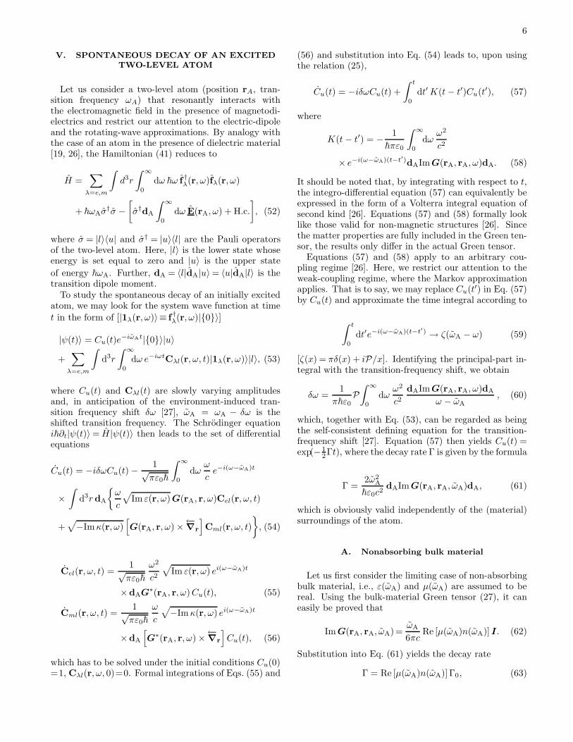
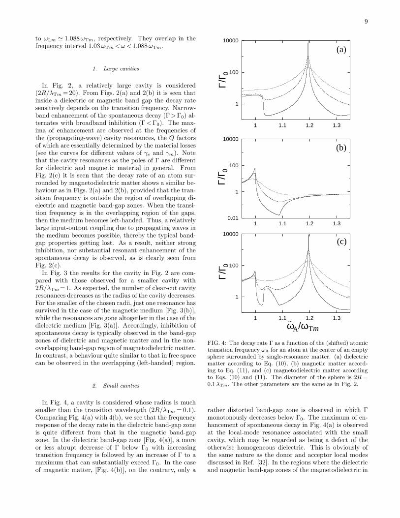
FIG. 3: The decay rate Γ as a function of the (shifted) atomictransition frequency ωA for an atom at the center of an emptysphere surrounded by single-resonance matter. (a) dielectricmatter according to Eq. (10), (b) magnetic matter accordingto Eq. (11), and (c) magnetodielectric matter according toEqs. (10) and (11) [γe/ωTm = γm/ωTm = 0.001, the otherparameters are the same as in Fig. 2]. The values of thesphere diameter are 2R = 20 λTm (dashed lines) and 2R =1λTm (solid lines).

quency for the case of the cavity being surrounded by(a) purely dielectric matter, (b) purely magnetic mat-ter, and (c) magnetodielectric matter near the band-gapzones. The permittivity and permeability are given byEqs. (10) and (11), respectively. In the figures, the di-electric and magnetic band gaps are assumed to extendfrom ωTe = 1.03ωTm to ωLe≃ 1.274ωTm and from ωTm

9

to ωLm ≃ 1.088ωTm, respectively. They overlap in thefrequency interval 1.03ωTm<ω< 1.088ωTm.

1. Large cavities

In Fig. 2, a relatively large cavity is considered(2R/λTm =20). From Figs. 2(a) and 2(b) it is seen thatinside a dielectric or magnetic band gap the decay ratesensitively depends on the transition frequency. Narrow-band enhancement of the spontaneous decay (Γ>Γ0) al-ternates with broadband inhibition (Γ<Γ0). The max-ima of enhancement are observed at the frequencies ofthe (propagating-wave) cavity resonances, the Q factorsof which are essentially determined by the material losses(see the curves for different values of γe and γm). Notethat the cavity resonances as the poles of Γ are differentfor dielectric and magnetic material in general. FromFig. 2(c) it is seen that the decay rate of an atom sur-rounded by magnetodielectric matter shows a similar be-haviour as in Figs. 2(a) and 2(b), provided that the tran-sition frequency is outside the region of overlapping di-electric and magnetic band-gap zones. When the transi-tion frequency is in the overlapping region of the gaps,then the medium becomes left-handed. Thus, a relativelylarge input-output coupling due to propagating waves inthe medium becomes possible, thereby the typical band-gap properties getting lost. As a result, neither stronginhibition, nor substantial resonant enhancement of thespontaneous decay is observed, as is clearly seen fromFig. 2(c).

In Fig. 3 the results for the cavity in Fig. 2 are com-pared with those observed for a smaller cavity with2R/λTm =1. As expected, the number of clear-cut cavityresonances decreases as the radius of the cavity decreases.For the smaller of the chosen radii, just one resonance hassurvived in the case of the magnetic medium [Fig. 3(b)],while the resonances are gone altogether in the case of thedielectric medium [Fig. 3(a)]. Accordingly, inhibition ofspontaneous decay is typically observed in the band-gapzones of dielectric and magnetic matter and in the non-overlapping band-gap region of magnetodielectric matter.In contrast, a behaviour quite similar to that in free spacecan be observed in the overlapping (left-handed) region.

2. Small cavities

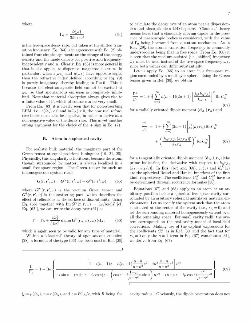
In Fig. 4, a cavity is considered whose radius is muchsmaller than the transition wavelength (2R/λTm = 0.1).Comparing Fig. 4(a) with 4(b), we see that the frequencyresponse of the decay rate in the dielectric band-gap zoneis quite different from that in the magnetic band-gapzone. In the dielectric band-gap zone [Fig. 4(a)], a moreor less abrupt decrease of Γ below Γ0 with increasingtransition frequency is followed by an increase of Γ to amaximum that can substantially exceed Γ0. In the caseof magnetic matter, [Fig. 4(b)], on the contrary, only a

1

100

10000

1 1.1 1.2 1.3

0.01

1

100

10000

1 1.1 1.2 1.3

1

100

10000

1 1.1 1.2 1.3

(a)

(b)

(c)

ω /ω

Γ/Γ

Γ/Γ

Γ/Γ

00

0

A Tm~

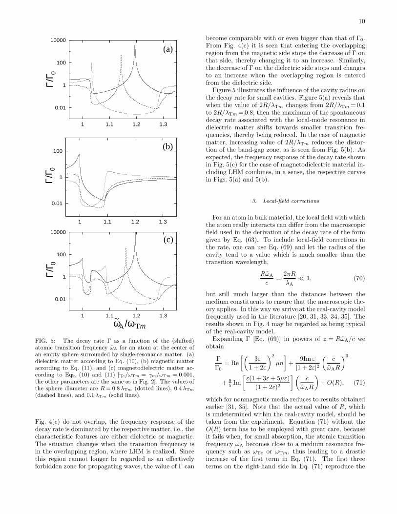
FIG. 4: The decay rate Γ as a function of the (shifted) atomictransition frequency ωA for an atom at the center of an emptysphere surrounded by single-resonance matter. (a) dielectricmatter according to Eq. (10), (b) magnetic matter accord-ing to Eq. (11), and (c) magnetodielectric matter accordingto Eqs. (10) and (11). The diameter of the sphere is 2R =0.1 λTm. The other parameters are the same as in Fig. 2.

rather distorted band-gap zone is observed in which Γmonotonously decreases below Γ0. The maximum of en-hancement of spontaneous decay in Fig. 4(a) is observedat the local-mode resonance associated with the smallcavity, which may be regarded as being a defect of theotherwise homogeneous dielectric. This is obviously ofthe same nature as the donor and acceptor local modesdiscussed in Ref. [32]. In the regions where the dielectricand magnetic band-gap zones of the magnetodielectric in

10

0.01

1

100

10000

1 1.1 1.2 1.3

0.01

1

100

1 1.1 1.2 1.3

0.01

1

100

10000

1 1.1 1.2 1.3

(a)

(b)

(c)

ω /ω

Γ/Γ

Γ/Γ

Γ/Γ

00

0

A T~

m

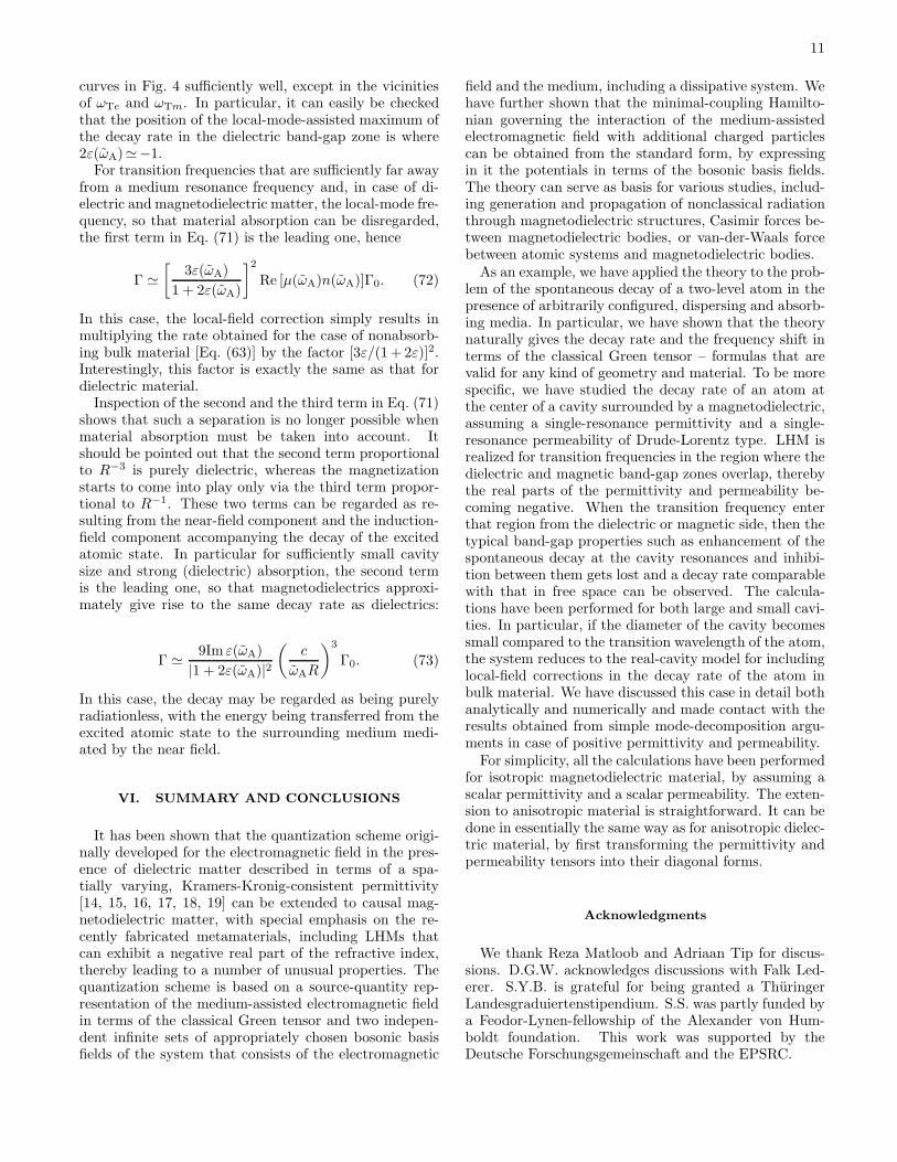
FIG. 5: The decay rate Γ as a function of the (shifted)atomic transition frequency ωA for an atom at the center ofan empty sphere surrounded by single-resonance matter. (a)dielectric matter according to Eq. (10), (b) magnetic matteraccording to Eq. (11), and (c) magnetodielectric matter ac-cording to Eqs. (10) and (11) [γe/ωTm = γm/ωTm = 0.001,the other parameters are the same as in Fig. 2]. The values ofthe sphere diameter are R = 0.8λTm (dotted lines), 0.4 λTm

(dashed lines), and 0.1 λTm (solid lines).

Fig. 4(c) do not overlap, the frequency response of thedecay rate is dominated by the respective matter, i.e., thecharacteristic features are either dielectric or magnetic.The situation changes when the transition frequency isin the overlapping region, where LHM is realized. Sincethis region cannot longer be regarded as an effectivelyforbidden zone for propagating waves, the value of Γ can

become comparable with or even bigger than that of Γ0.From Fig. 4(c) it is seen that entering the overlappingregion from the magnetic side stops the decrease of Γ onthat side, thereby changing it to an increase. Similarly,the decrease of Γ on the dielectric side stops and changesto an increase when the overlapping region is enteredfrom the dielectric side.

Figure 5 illustrates the influence of the cavity radius onthe decay rate for small cavities. Figure 5(a) reveals thatwhen the value of 2R/λTm changes from 2R/λTm =0.1to 2R/λTm =0.8, then the maximum of the spontaneousdecay rate associated with the local-mode resonance indielectric matter shifts towards smaller transition fre-quencies, thereby being reduced. In the case of magneticmatter, increasing value of 2R/λTm reduces the distor-tion of the band-gap zone, as is seen from Fig. 5(b). Asexpected, the frequency response of the decay rate shownin Fig. 5(c) for the case of magnetodielectric material in-cluding LHM combines, in a sense, the respective curvesin Figs. 5(a) and 5(b).

3. Local-field corrections

For an atom in bulk material, the local field with whichthe atom really interacts can differ from the macroscopicfield used in the derivation of the decay rate of the formgiven by Eq. (63). To include local-field corrections inthe rate, one can use Eq. (69) and let the radius of thecavity tend to a value which is much smaller than thetransition wavelength,

RωA

c=

2πR

λA≪ 1, (70)

but still much larger than the distances between themedium constituents to ensure that the macroscopic the-ory applies. In this way we arrive at the real-cavity modelfrequently used in the literature [20, 31, 33, 34, 35]. Theresults shown in Fig. 4 may be regarded as being typicalof the real-cavity model.

Expanding Γ [Eq. (69)] in powers of z = RωA/c weobtain

Γ

Γ0= Re

[(

3ε

1 + 2ε

)2

µn

]

+9Im ε

|1 + 2ε|2(

c

ωAR

)3

+ 95 Im

[

ε(1 + 3ε+ 5µε)

(1 + 2ε)2

] (

c

ωAR

)

+O(R), (71)

which for nonmagnetic media reduces to results obtainedearlier [31, 35]. Note that the actual value of R, whichis undetermined within the real-cavity model, should betaken from the experiment. Equation (71) without theO(R) term has to be employed with great care, becauseit fails when, for small absorption, the atomic transitionfrequency ωA becomes close to a medium resonance fre-quency such as ωTe or ωTm, thus leading to a drasticincrease of the first term in Eq. (71). The first threeterms on the right-hand side in Eq. (71) reproduce the

11

curves in Fig. 4 sufficiently well, except in the vicinitiesof ωTe and ωTm. In particular, it can easily be checkedthat the position of the local-mode-assisted maximum ofthe decay rate in the dielectric band-gap zone is where2ε(ωA)≃−1.

For transition frequencies that are sufficiently far awayfrom a medium resonance frequency and, in case of di-electric and magnetodielectric matter, the local-mode fre-quency, so that material absorption can be disregarded,the first term in Eq. (71) is the leading one, hence

Γ ≃[

3ε(ωA)

1 + 2ε(ωA)

]2

Re [µ(ωA)n(ωA)]Γ0. (72)

In this case, the local-field correction simply results inmultiplying the rate obtained for the case of nonabsorb-ing bulk material [Eq. (63)] by the factor [3ε/(1 + 2ε)]2.Interestingly, this factor is exactly the same as that fordielectric material.

Inspection of the second and the third term in Eq. (71)shows that such a separation is no longer possible whenmaterial absorption must be taken into account. Itshould be pointed out that the second term proportionalto R−3 is purely dielectric, whereas the magnetizationstarts to come into play only via the third term propor-tional to R−1. These two terms can be regarded as re-sulting from the near-field component and the induction-field component accompanying the decay of the excitedatomic state. In particular for sufficiently small cavitysize and strong (dielectric) absorption, the second termis the leading one, so that magnetodielectrics approxi-mately give rise to the same decay rate as dielectrics:

Γ ≃ 9Im ε(ωA)

|1 + 2ε(ωA)|2(

c

ωAR

)3

Γ0. (73)

In this case, the decay may be regarded as being purelyradiationless, with the energy being transferred from theexcited atomic state to the surrounding medium medi-ated by the near field.

VI. SUMMARY AND CONCLUSIONS

It has been shown that the quantization scheme origi-nally developed for the electromagnetic field in the pres-ence of dielectric matter described in terms of a spa-tially varying, Kramers-Kronig-consistent permittivity[14, 15, 16, 17, 18, 19] can be extended to causal mag-netodielectric matter, with special emphasis on the re-cently fabricated metamaterials, including LHMs thatcan exhibit a negative real part of the refractive index,thereby leading to a number of unusual properties. Thequantization scheme is based on a source-quantity rep-resentation of the medium-assisted electromagnetic fieldin terms of the classical Green tensor and two indepen-dent infinite sets of appropriately chosen bosonic basisfields of the system that consists of the electromagnetic

field and the medium, including a dissipative system. Wehave further shown that the minimal-coupling Hamilto-nian governing the interaction of the medium-assistedelectromagnetic field with additional charged particlescan be obtained from the standard form, by expressingin it the potentials in terms of the bosonic basis fields.The theory can serve as basis for various studies, includ-ing generation and propagation of nonclassical radiationthrough magnetodielectric structures, Casimir forces be-tween magnetodielectric bodies, or van-der-Waals forcebetween atomic systems and magnetodielectric bodies.

As an example, we have applied the theory to the prob-lem of the spontaneous decay of a two-level atom in thepresence of arbitrarily configured, dispersing and absorb-ing media. In particular, we have shown that the theorynaturally gives the decay rate and the frequency shift interms of the classical Green tensor – formulas that arevalid for any kind of geometry and material. To be morespecific, we have studied the decay rate of an atom atthe center of a cavity surrounded by a magnetodielectric,assuming a single-resonance permittivity and a single-resonance permeability of Drude-Lorentz type. LHM isrealized for transition frequencies in the region where thedielectric and magnetic band-gap zones overlap, therebythe real parts of the permittivity and permeability be-coming negative. When the transition frequency enterthat region from the dielectric or magnetic side, then thetypical band-gap properties such as enhancement of thespontaneous decay at the cavity resonances and inhibi-tion between them gets lost and a decay rate comparablewith that in free space can be observed. The calcula-tions have been performed for both large and small cavi-ties. In particular, if the diameter of the cavity becomessmall compared to the transition wavelength of the atom,the system reduces to the real-cavity model for includinglocal-field corrections in the decay rate of the atom inbulk material. We have discussed this case in detail bothanalytically and numerically and made contact with theresults obtained from simple mode-decomposition argu-ments in case of positive permittivity and permeability.

For simplicity, all the calculations have been performedfor isotropic magnetodielectric material, by assuming ascalar permittivity and a scalar permeability. The exten-sion to anisotropic material is straightforward. It can bedone in essentially the same way as for anisotropic dielec-tric material, by first transforming the permittivity andpermeability tensors into their diagonal forms.

Acknowledgments

We thank Reza Matloob and Adriaan Tip for discus-sions. D.G.W. acknowledges discussions with Falk Led-erer. S.Y.B. is grateful for being granted a ThuringerLandesgraduiertenstipendium. S.S. was partly funded bya Feodor-Lynen-fellowship of the Alexander von Hum-boldt foundation. This work was supported by theDeutsche Forschungsgemeinschaft and the EPSRC.

12

APPENDIX A: SOME PROPERTIES OF THE

GREEN TENSOR

Following Ref. [19], we regard the Green tensor as be-ing the matrix elements in the position basis of a tensor-valued Green operator G = G(ω) in an abstract single-

particle Hilbert space, G(r, r′, ω) = 〈r|G|r′〉, so thatEq. (23) can be regarded as the position-representation

of the operator equation HG = I, where

H = −p× κ(r, ω)p×−ω2

c2ε(r, ω)I. (A1)

Using the relations 〈r|r|r′〉 = rδ(r − r′), 〈r|p|r′〉 =

−i∇δ(r− r′), and 〈r|I|r′〉= δ(r− r′), we have

H(r, r′, ω) ≡ 〈r|H |r′〉

= ∇×κ(r, ω)∇× δ(r−r′)− ω2

c2ε(r, ω)δ(r−r′), (A2)

which in Cartesian coordinates reads

Hij(r, r′, ω) =

{

∂rj κ(r, ω)∂r

i

−[

∂rl κ(r, ω)∂r

l +ω2

c2ε(r, ω)

]

δij

}

δ(r− r′). (A3)

Since H is injective and thus an invertible one-to-onemap between vector functions, we can write G = H−1.Multiplying this equation by H from the right, we have

GH = I, (A4)

which in the position basis reads∫

d3s 〈r|G|s〉〈s|H |r′〉 = δ(r− r′). (A5)

Recalling Eq. (A3), we derive, on integrating by partsand taking into account that the Green tensor vanishesat infinity,∫

d3sGik(r, s, ω)Hkj(s, r′, ω)

=

{

∂r′

k κ(r′, ω)∂r′

j −[

∂r′

l κ(r′, ω)∂r′

l +ω2

c2ε(r′, ω)

]

δkj

}

×Gik(r, r′, ω) = δij(r− r′). (A6)

Interchanging the vector indices i and j and the spatialarguments r and r′, we obtain

{

∂rkκ(r, ω)∂r

i −[

∂rl κ(r, ω)∂r

l +ω2

c2ε(r, ω)

]

δki

}

×Gjk(r′, r, ω) = δij(r − r′), (A7)

which, according to Eq. (23), is just the defining equationfor Gkj(r, r

′, ω). Thus, the reciprocity relation (24) isproved valid.

To prove the integral relation (25), we introduce oper-

ators O‡ by(

O‡)

ij=

(

Oji

)†= O†

ji. From Eq. (A4) it

then follows that

H‡G

‡ = I. (A8)

Multiplying Eq. (A4) from the right by G‡ and Eq. (A8)

from the left by G and subtracting the resulting equa-tions from each other, we obtain

G(

H − H‡)

G‡ = G

‡ − G, (A9)

which in the position basis reads

∫

d3s

∫

d3s′Gim(r, s, ω)[Hmn(s, s′, ω)

−H∗nm(s′, s, ω)]G∗

nj(s′, r′, ω) = −2iImGij(r, r

′, ω).

(A10)

Note that 〈r|H‡mn|r′〉 = H∗

nm(r′, r, ω) and 〈r|G‡ij |r′〉 =

G∗ji(r

′, r, ω). Inserting Eq. (A3) into Eq. (A10), aftersome manipulation we derive

∫

d3s{

Imκ (s, ω)∂snGim(r, s, ω)

× [∂smG

∗nj(s, r

′, ω)− ∂snG

∗mj(s, r

′, ω)]

+ω2

c2Im ε(s, ω)Gim(r, s, ω)G∗

mj(s, r′, ω)

}

= ImGij(r, r′, ω), (A11)

which is just Eq. (25) in Cartesian coordinates.To examine the asymptotic behaviour of the Green ten-

sor in the upper half of the complex ω-plane as |ω| → ∞and |ω| → 0, we introduce the tensor-valued projectors

I⊥ = I − I

‖, I‖ =

p⊗ p

p2(A12)

[note that 〈r|I⊥(‖)|r′〉=δ⊥(‖)(r− r′)], and decompose G

as [19],

G = H−1 = I

‖(I‖HI

‖)−1I‖

+[

I⊥ − I

‖(I‖HI

‖)−1I‖HI

⊥]

K

×[

I⊥ − I

⊥HI

‖(I‖HI

‖)−1I‖]

, (A13)

where

K =[

I⊥

HI⊥ − I

⊥HI

‖(I‖HI

‖)−1I‖HI

⊥]−1

. (A14)

Recalling that ε(r, ω), µ(r, ω)→ 1 as |ω| →∞, we easily

see that the high-frequency limits of H and G are thesame as for dielectric material, thus [19]

lim|ω|→∞

ω2

c2G(r, r′, ω) = −δ(r− r′). (A15)

13

To find the low-frequency limit of G, we note that thesecond term in Eq. (A13) is regular. To study the firstterm, we distinguish between two cases.(i) The first term of H in Eq. (A1) is transverse,

−I‖p× κ(r, ω)p× = −p× κ(r, ω)p× I

‖ = 0, (A16)

and therefore does not contribute to I‖HI‖. It thenfollows that the same low-frequency behaviour as in thecase of dielectric matter is observed, thus [19]

lim|ω|→0

ω2

c2G = −I

‖[I‖ε(r, ω = 0)I‖]−1I‖, (A17)

i.e., because ε(r, ω = 0) 6= 0,

lim|ω|→0

ω2

c2G(r, r′, ω) = M , Mij <∞. (A18)

(ii) Equation (A16) is not valid, so that the first

term of H in Eq. (A1) contributes to I‖HI

‖. Sinceµ(r, ω = 0) 6=0 [thus κ(r, ω=0) being finite], we find that

lim|ω|→0

G(r, r′, ω) = N , Nij <∞. (A19)

APPENDIX B: COMMUTATION RELATIONS

By using Eqs. (22), (32), the commutation relations(30) and (31), and the integral relation (25), we derive

[

Ei(r, ω), E†

j(r′, ω′)

]

=~ω2

πε0c2ImGij(r, r

′, ω) δ(ω − ω′), (B1)

[

Ei(r, ω), Ej(r′, ω′)

]

=[

E†

i (r, ω), E†

j(r′, ω′)

]

= 0. (B2)

From Eqs. (34), (B1), and (B2) it is easily seen that thecommutation relations (35) are valid. Moreover, we findthat, on recalling that G∗(r, r′, ω) = G(r, r′,−ω∗),

[

ε0Ei(r), Aj(r′)

]

=

∫

d3s

[

2i~

π

∫ ∞

0

dωω

c2ImGik(r, s, ω)

]

δ⊥kj(s− r′)

=

∫

d3s

[

~

πP

∫ ∞

−∞

dωω

c2Gik(r, s, ω)

]

δ⊥kj(s− r′)

=~

πP

∫ ∞

−∞

dω

ω

ω2

c2〈r|GI

⊥|r′〉ij (B3)

(P , principal part). Since the Green tensor is analytic inthe upper half of the complex ω-plane with the asymp-totic behaviour according to Eq. (A15), the frequencyintegral in Eq. (B3) can be evaluated by contour integra-tion along an infinitely small half-circle around ω=0, and

along an infinitely large half-circle |ω|→∞. Taking intoaccount that the Green tensor either has only longitudi-nal components in the limit |ω| → 0, cf. Eq. (A17), and

hence ω/cGI⊥→0, or is well-behaved, cf. Eq. (A19), wesee that the integral along the infinitely small half-circlevanishes. Recalling Eq. (A15), we then readily find

[

ε0Ei(r), Aj(r′)

]

= i~δ⊥ij(r− r′). (B4)

Since B(r) = ∇× A(r), from Eq. (B4) it follows that

[

ε0Ei(r), Bj(r′)

]

=−i~ǫijk∂rkδ(r− r′), (B5)

i.e., Eq. (36). It is then not difficult to see that thecommutation relation (B4) implies

[

ϕ(r), Ai(r′)

]

=[

ϕ(r), Bi(r′)

]

= 0. (B6)

To evaluate commutators involving the displacementfield and the magnetic field, recall Eqs. (16) – (19). Usingthe relations presented above, we derive

[

Di(r), Dj(r′)

]

= 0, (B7)[

Hi(r), Hj(r′)

]

= 0, (B8)

and

[

Di(r), µ0Hj(r′)

]

= −i~ǫijk∂rkδ(r− r′). (B9)

Note that Eq. (B9) follows by using similar arguments asin the derivation of Eq. (B4) from Eq. (B3). A similarcalculation leads to

[

Di(r), Aj(r′)

]

= i~δ⊥ij(r− r′), (B10)[

Hi(r), Aj(r′)

]

=[

Di(r), ϕ(r′)]

=[

Hi(r), ϕ(r′)]

= 0.

(B11)

By combining Eqs. (B10) – (B11) with Eqs. (B4) and(B6), it is not difficult to verify that polarization andmagnetization commute with the introduced potentialsas well as among themselves.

APPENDIX C: HEISENBERG EQUATIONS OF

MOTION

By using the Hamiltonian (41) and recalling the def-initions of the medium-assisted field quantities in terms

of the basic fields fλi(r, ω) the basic-field commutationrelations (30) and (31), the commutation relations thathave been derived from them, and the standard commu-tation relations for the particle coordinates and canonicalmomenta, it is straightforward to prove that the theoryyields both the correct Maxwell equations (47) and (48)and the correct Newtonian equation of motion (51).

Let us begin with the Maxwell equations. We deriveon recalling Eqs. (40) and (34) together with Eqs. (22)

14

and (32) and the commutation relations (30) and (31),

˙~B(r, t) =

1

i~

[

~B(r, t), H]

= ∇×∫ ∞

0

dω1

i~

[

A(r, ω), H]

+ H.c.

=−∇× E(r) = −∇× ~E(r), (C1)

which is Eq. (47). To derive the equation of motion forthe displacement field, we have to consider several com-mutators according to

˙~D(r) =

1

i~

[

~D(r, t), H]

=1

i~

∫

d3r′∫ ∞

0

dω ~ω∑

λ=e,m

[

D(r), f†λ(r′, ω)fλ(r′, ω)]

+1

i~

∑

α

1

2mα

[

D(r),[

pα − qαA(rα)]2

]

− ε0i~

∑

α

1

2mα

[

∇ϕA(r),[

pα − qαA(rα)]2

]

. (C2)

The first commutator in Eq. (C2) can easily be foundby recalling the definitions of displacement and magneticfields as

1

i~

∫

d3r′∫ ∞

0

dω ~ω∑

λ=e,m

[

D(r), f†λ(r′, ω)fλ(r′, ω)]

= −∫ ∞

0

dω iωD(r, ω) + H.c. = ∇× ~H(r). (C3)

Applying the commutation relation (B10), and recallingthe definition of the current density, we find that thesecond term on the right-hand side of Eq. (C2) can bewritten as

1

i~

∑

α

1

2mα

[

D(r),[

pα − qαA(rα)]2

]

= −j⊥A(r), (C4)

where the Newtonian equation of motion (50) has beenused which follows directly from the Hamiltonian (41).Finally, standard commutation relations together withthe definitions of the scalar potential, Eqs. (42) and (43),and the current density, Eq. (49) together with Eq. (50),lead to

−ε0i~

∑

α

1

2mα[∇ϕA(r), [pα − qαA(rα)]2] = −j

‖A(r).

(C5)Inserting Eqs. (C3) – (C5) into Eq. (C2), we arrive atEq. (48).

In order to prove Eq. (51), we consider the equation

mα¨rα =

1

i~

[

pα − qαA(rα), H]

= −qαi~

∫

d3r

∫ ∞

0

dω ~ω∑

λ=e,m

[

A(rα), f†λ(r, ω)fλ(r, ω)]

+1

i~

∑

β

1

2mβ

[

pα − qαA(rα),[

pβ − qβA(rβ)]2

]

+1

2i~

∫

d3r[

pα, ρA(r)ϕA(r)]

+1

i~

∫

d3r[

pα, ρA(r)ϕ(r)]

. (C6)

The first term on the right-hand side of Eq. (C6) is again

−qαi~

∫

d3r

∫ ∞

0

dω ~ω∑

λ=e,m

[

A(rα), f†λ(r, ω)fλ(r, ω)]

= iωqαA(rα) = qαE⊥(rα). (C7)

The second term gives rise to two terms,

1

i~

∑

β

1

2mβ

[

pα,[

pβ − qβA(rβ)]2

]

= 12qα

{

˙rαA(rα)⊗←−∇ + ∇⊗ A(rα) ˙rα

}

(C8)

and

−qαi~

∑

β

1

2mβ

[

A(rα),[

pβ − qβA(rβ)]2

]

= − 12qα

{

˙rα∇⊗ A(rα) + A(rα)⊗ ˙rα←−∇

}

, (C9)

and thus

1

i~

∑

β

1

2mβ

[

pα − qαA(rα),[

pβ − qβA(rβ)]2

]

= 12qα

[

˙rα × ~B(rα)− ~B(rα)× ˙rα

]

. (C10)

By means of Eqs. (39) and (42) one can see that the lasttwo terms in Eq. (C6) can be rewritten as

1

2i~

∫

d3r[

pα, ρA(r)ϕA(r)]

= −qα∇ϕA(rα), (C11)

1

i~

∫

d3r[

pα, ρA(r)ϕ(r)]

= qαE‖(rα). (C12)

Inserting Eqs. (C7), (C10) – (C12) into Eq. (C6) andmaking use of Eq. (44), we just arrive at Eq. (51).

15

[1] V. G. Veselago, Sov. Phys. Usp. 10, 509 (1968).[2] D. R. Smith, W. J. Padilla, D. C. Vier, S. C. Nemat-

Nasser, S. Shultz, Phys. Rev. Lett. 84, 4184 (2000); R.A. Shelby, D. R. Smith, S. C. Nemat-Nasser, S. Shultz,Appl. Phys. Lett. 78, 489 (2001).

[3] R. A. Shelby, D. R. Smith, and S. Shultz, Science 292,77 (2001).

[4] R. Marques, J. Martel, F. Mesa, and F. Medina, Phys.Rev. Lett. 89, 183901 (2002)

[5] A. Grbic and G. V. Eleftheriades, J. Appl. Phys. 92, 5930(2002).

[6] C. G. Parazzoli, R. B. Greegor, K. Li, B. E. C. Koltenbah,and M. Tanielian, Phys. Rev. Lett. 90, 107401 (2003); K.Li, S. J. McLean, R. B. Greegor, C. G. Parazzoli, and M.H. Tanielian, App. Phys. Lett. 82, 2535 (2003); A. A.Houck, J. B. Brock, and I. L. Chuang, Phys. Rev. Lett.90, 137401 (2003).

[7] L. V. Panina, A. N. Grigorenko, and D. P. Makhnovskiy,Phys. Rev. B 66, 155411 (2002).

[8] M. L. Povinelli, S. G. Johnson, J. D. Joannopoulos, andJ. B. Pendry, Appl. Phys. Lett. 82, 1069 (2003).

[9] D. R. Smith and N. Kroll, Phys. Rev. Lett. 85, 2933(2000).

[10] J. B. Pendry, Phys. Rev. Lett. 85, 3966 (2000).[11] G. W. ’t Hooft, Phys. Rev. Lett. 87, 249701 (2001); J.

B. Pendry, ibid., 249702 (2001); J. M. Williams, ibid.,249703 (2001); J. B. Pendry, ibid., 249704 (2001); P.Markos and C. M. Soukoulis, Phys. Rev. B 65, 033401(2001); P. Markos, I. Rousochatzakis, and C. M. Souk-oulis, Phys. Rev. E 66, 045601(R) (2002); P. M. Valanju,R. M. Walser, and A. P. Valanju, Phys. Rev. Lett. 88,187401 (2002); A. L. Pokrovsky and A. L. Efros, ibid. 89,093901 (2002); J. Pacheco, Jr., T. M. Grzegorczyk, B.-I.Wu, Y. Zhang, and J. A. Kong, ibid., 257401 (2002); N.Fang and X. Zhang, Appl. Phys. Lett. 82, 161 (2003); G.Gomez-Santos, Phys. Rev. Lett. 90, 077401 (2003); D.R. Smith and D. Schurig, ibid., 077405 (2003); J. Li, L.Zhou, C. T. Chan, and P. Sheng, ibid., 083901 (2003);S. Foteinopoulou, E. N. Economou, and C. M. Soukoulis,ibid., 107402 (2003); S. A. Cummer, Appl. Phys. Lett. 82,1503 (2003); ibid., 2008 (2003); D. R. Smith, D. Schurig,M. Rosenbluth, and S. Schultz, ibid., 1506 (2003); P. F.Loschialpo, D. L. Smith, D. W. Forester, F. J. Rachford,and J. Schelleng, Phys. Rev. E 67, 025602 (2003).

[12] R. W. Ziolkowski and E. Heyman, Phys. Rev. E 64,056625 (2001).

[13] N. Garcia and M. Nieto-Vesperinas, Phys. Rev. Lett. 88,207403 (2002); Opt. Lett. 27, 885 (2002).

[14] T. Gruner and D.-G. Welsch, Third Workshop on Quan-

tum Field Theory under the Influence of External Condi-

tions (Leipzig, 1995) [B.G. Teubner Verlagsgesellschaft,Stuttgart·Leipzig, 1996]; Phys. Rev. A 53, 1818 (1996).

[15] R. Matloob, R. Loudon, S.M. Barnett, and J. Jeffers,Phys. Rev. A 52, 4823 (1995); R. Matloob and R.Loudon, ibid. 53, 4567 (1996).

[16] Ho Trung Dung, L. Knoll, and D.-G. Welsch, Phys. Rev.A 57, 3931 (1998); S. Scheel, L. Knoll, and D.-G. Welsch,ibid. 58, 700 (1998).

[17] A. Tip, Phys. Rev. A 56, 5022 (1997); ibid. 57, 4818(1998); A. Tip, L. Knoll, S. Scheel, and D.-G. Welsch,ibid. 63, 043806 (2001).

[18] O. D. Stefano, S. Savasta, and R. Girlanda, Phys. Rev.A 61, 023803 (2000).

[19] L. Knoll, S. Scheel, and D.-G. Welsch, in Coherence and

Statistics of Photons and Atoms, edited by J. Perina(John Wiley & Son, New York, 2001) p. 1; e-printquant-ph/0006121.

[20] E. Yablonovitch, T. J. Gmitter, and R. Blatt, Phys. Rev.Lett. 61, 2546 (1988).

[21] S. M. Barnett, B. Huttner, R. Loudon, and R. Matloob,J. Phys. A 29, 3763 (1996).

[22] L. D. Landau and E. M. Lifshitz, Electrodynamics of

Continuous Media (Pergamon Press, 1960).[23] R. Ruppin, Phys. Lett. A 299, 309 (2002).[24] J. B. Pendry, A. J. Holden, D. J. Robbins, and W. J.

Stewart, IEEE Trans. Microwave Theory Tech. 47, 2075(1999).

[25] A.A. Abrikosov, L.P. Gorkov, and I.E. DzyaloshinskiMethods of Quantum Field Theory in Statistical Physics

(Dover, New York, 1963).[26] Ho Trung Dung, L. Knoll, and D.-G. Welsch, Phys. Rev.

A 62, 053804 (2000); in Recent Research Developments

in Optics, Vol. 1 (Research Signpost, Trivandrum, India,2001) p. 225.

[27] Ho Trung Dung, L. Knoll, and D.-G. Welsch, Phys. Rev.A 66, 063810 (2002).

[28] R.R. Chance, A.Prock, and R. Sylbey, Adv. Chem. Phys.37, 1 (1978).

[29] V. V. Klimov, Opt. Commun. 211, 183 (2002).[30] L. W. Li, P. S. Kooi, M. S. Leong, and T. S. Yeo, IEEE

Trans. Microwave Theory Tech. 42, 2302 (1994); C.-T.Tai, Dyadic Green Functions in Electromagnetic Theory

(IEEE Press, New York, 1994).[31] S. Scheel, L. Knoll, and D.-G. Welsch, Phys. Rev. A 60,

4094 (1999).[32] E. Yablonovitch, T. J. Gmitter, R. D. Meade, A. M.

Rappe, K. D. Brommer, and J. D. Joannopoulos, Phys.Rev. Lett. 67, 3380 (1991).

[33] L. Onsager, J. Am. Chem. Soc. 58, 1486 (1936).[34] R.J. Glauber and M. Lewenstein, Phys. Rev. A 43, 467

(1991).[35] M. S. Tomas, Phys. Rev. A 63, 053811 (2001).