Cumulative and Averaging Fusion of Beliefs

Audun Jøsang a Javier Diaz b Maria Rifqi b

aUNIK Graduate Center, University of Oslo, Norwayjosang@unik.no

bCNRS - UMR 7606 LIP6, Universite Paris VI, France{Javier.Diaz, Maria.Rifqi}@lip6.fr

Abstract

The problem of fusing beliefs in the Dempster-Shafer belief theory has attracted consid-erable attention over the last two decades. The classical Dempster’s Rule has often beencriticised, and many alternative rules for belief fusion have been proposed in the literature.We show that it is crucial to consider the nature of the situation to be modelled and to selectthe appropriate fusion operator as a function thereof. In this paper we present the cumula-tive and averaging fusion rules for belief functions, which represent generalisations of thesubjective logic cumulative and averaging fusion operators for opinions respectively. Thegeneralised operators are applicable to the combination of general basic belief assignments(bbas). These rules, which can be directly derived from classical statistical theory, produceresults that correspond well with human intuition.

Key words: Belief Theory, Subjective Logic, Fusion, Dempster’s Rule

1 Introduction

Belief theory has its origin in a model for upper and lower probabilities proposed byDempster in 1960. Shafer later used the same fundamental framework as a modelfor expressing beliefs [1]. The main idea behind the theory of belief functions is toabandon the additivity principle of probability theory, i.e. that the sum of probabil-ities on all pairwise disjoint possibilities always equals one. Instead belief theorygives observers the ability to assign belief masses to any subset of a state space, i.e.to non-disjoint possibilities including the whole state space itself. The advantage ofthis approach over classical probabilistic modelling is that uncertainty about subsetprobabilities, e.g. due to missing evidence, can be explicitly expressed. Uncertaintycan for example be expressed by assigning belief mass to the union of singletons, orto the whole state space itself. Consistency is preserved by requiring that the sum ofall belief masses always equals one. The difference between probability additivity

Preprint of article published in Information Fusion, 11(2), April 2010, p.192-200, Elsevier

and belief mass additivity is that for probabilities the states must all be mutuallydisjoint, whereas for belief masses the states can be overlapping. Shafer’s book [1]describes many characteristics of belief functions, but the two main elements are 1)a flexible way of expressing beliefs, and 2) a method for fusing beliefs, commonlyknown as Dempster’s Rule.

There are well known examples where Dempster’s rule produces counter-intuitiveresults, especially in case of strong conflict between the two argument beliefs. Moti-vated by this observation, numerous authors have proposed alternative methods forfusing beliefs, e.g. [2,3,4,5,6,7,8,9]. An overview of belief fusion rules that havebeen proposed in the literature is provided in [10]. These rules express differentbehaviours with respect to the results of fusing beliefs, but have in general beenproposed with the same basic purpose in mind: to fuse two beliefs into a singlebelief that reflects the two possibly conflicting beliefs in a fair and equal way.

However, situations that may seem similar at first glance can be very different whenexamined more closely, and will therefore require different fusion operators. Forexample, the right operator for modelling the strength of a chain is the principleof the weakest link. The right operator for modelling the strength of a relay swim-ming team is the average strength of each member. Applying the weakest swimmerprinciple to assess the overall strength of the relay team might represent an approx-imation, but it is incorrect in general, and would give very unreliable predictions.Similarly, applying the principle of average strength of the links in a chain to as-sess the overall strength of the chain might represent an approximation, but it isincorrect in general and could be fatal if life depended on it. The observation ofthese simple examples tells us that it is crucial to properly understand the situationat hand in order to find the correct model for analysing it.

In our view researchers in the belief theory community have not paid sufficientattention to analysing the actual situation to be modelled in order to determinewhether Dempster’s rule or any other fusion rule can be correctly applied. Instead,researchers have often tried to assess the merits of fusion operators based solely onalgebraic properties, such as commutativity and associativity, which do not repre-sent sufficient criteria for judging an operator’s applicability to a particular situa-tion. For example, no matter how solid the theoretic basis for the average operatoris, it will never represent a correct model for the strength of a chain.

In this article we present two belief fusion operators called the cumulative andaveraging rules of combining beliefs. These rules do not represent an alternativeor competitor to Dempster’s rule because they are applicable in different types ofsituations than Dempster’s rule.

The terms cumulative rule and averaging rule have explicitly been chosen in or-der to have descriptive names for the types of situations to which they apply. Thecumulative rule of combination is applicable to situations where independent be-

2

lief functions are combined as a function of accumulation of the evidence. Theaveraging rule of combination is applicable to situations where dependent belieffunctions are combined as a function of the average of the evidence. This is differ-ent from Dempster’s rule, where beliefs are combined by normalised conjunction.It can be shown that non-normalised conjunction corresponds to multiplication ofbelief functions, and normalised conjunction corresponds to a series of stochasticconstraints [11] represented by the argument belief functions. This difference willbe illustrated by examples below.

The cumulative and averaging rules can be applied to the combination of generalbelief functions, and represents a generalisation of cumulative and averaging fusionof opinions in subjective logic[5,12,13,14]. The cumulative rule itself is then simplyequivalent to the additive combination of Dirichlet distributions, and the averagingrule is simply equivalent to the average of Dirichlet distributions. This also providesan equivalence mapping between Dirichlet distributions and belief functions [15].In this way, belief fusion in the form of the cumulative and averaging rules is firmlybased on classical statistical theory.

2 Theory of Belief Functions

In this section several concepts of the Dempster-Shafer theory of evidence [1] arerecalled in order to introduce notations used throughout the article. The term frameof discernment is used in belief theory with the equivalent meaning of state spacefrom probability theory. A frame denoted by Θ = {θi; i = 1, · · ·k} represents afinite set of exhaustive and exclusive possible values for a state variable of interest.The terms states, elements or outcomes will be used to denote the state variable. Theframe can for example be the set of six possible outcomes of throwing a dice, sothat the (unknown) outcome of a particular instance of throwing the dice becomesthe state variable. A bba (basic belief assignment 1 ), denoted by m, is defined as abelief distribution function from the powerset 2Θ to [0, 1] satisfying:

m(∅) = 0 and∑x⊆Θ

m(θ) = 1 . (1)

Values of a bba are called belief masses. Each subset x ⊆ Θ such that m(x) > 0 iscalled a focal element of Θ.

From a bba m can be derived a set of non-additive belief functions Bel: 2Θ → [0, 1],defined as:

Bel(x) �∑

∅�=y⊆x

m(y) ∀ x ⊆ Θ . (2)

1 Called basic probability assignment in [1], and Belief Mass Assignment (BMA) in [16,5].

3

The quantity Bel(x) can be interpreted as a measure of one’s total belief committedto the hypothesis that x is true. Note that functions m and Bel are in one-to-onecorrespondence [1] and can be seen as two facets of the same piece of information.

A few special classes of bba can be mentioned. A vacuous bba has m(Θ) = 1,i.e. no belief mass committed to any proper subset of Θ. A Bayesian bba is whenall the focal elements are singletons, i.e. one-element subsets of Θ. If all the focalelements are nestable (i.e. linearly ordered by inclusion) then we speak about aconsonant bba. A dogmatic bba is defined by Smets as a bba for which m(Θ) = 0.Let us note, that trivially, every Bayesian bba is dogmatic.

The powerset of the frame Θ is defined as 2Θ = {xi; xi ⊆ Θ}. We will define thestate space X as a special representation of the powerset of Θ. More precisely, theset X is defined as:

X = 2Θ\Θ (3)

meaning that all proper subsets of Θ are elements of X . By considering X as aframe in itself, a general bba on Θ becomes a particular bba on X called a Dirich-let bba. A belief mass on a proper subset of Θ then becomes a belief mass on asingleton of X . In addition we define m(X) = m(Θ). In this way, a Dirichlet bbaon X derived from a general bba on Θ, is characterised by having mutually dis-joint focal elements, except the whole frame X itself. This is formally defined asfollows.

Definition 1 (Dirichlet bba) Let X be a frame of discernment. A bba where theonly focal elements are X and/or singletons of X , is called a Dirichlet belief massdistribution function, or Dirichlet bba for short.

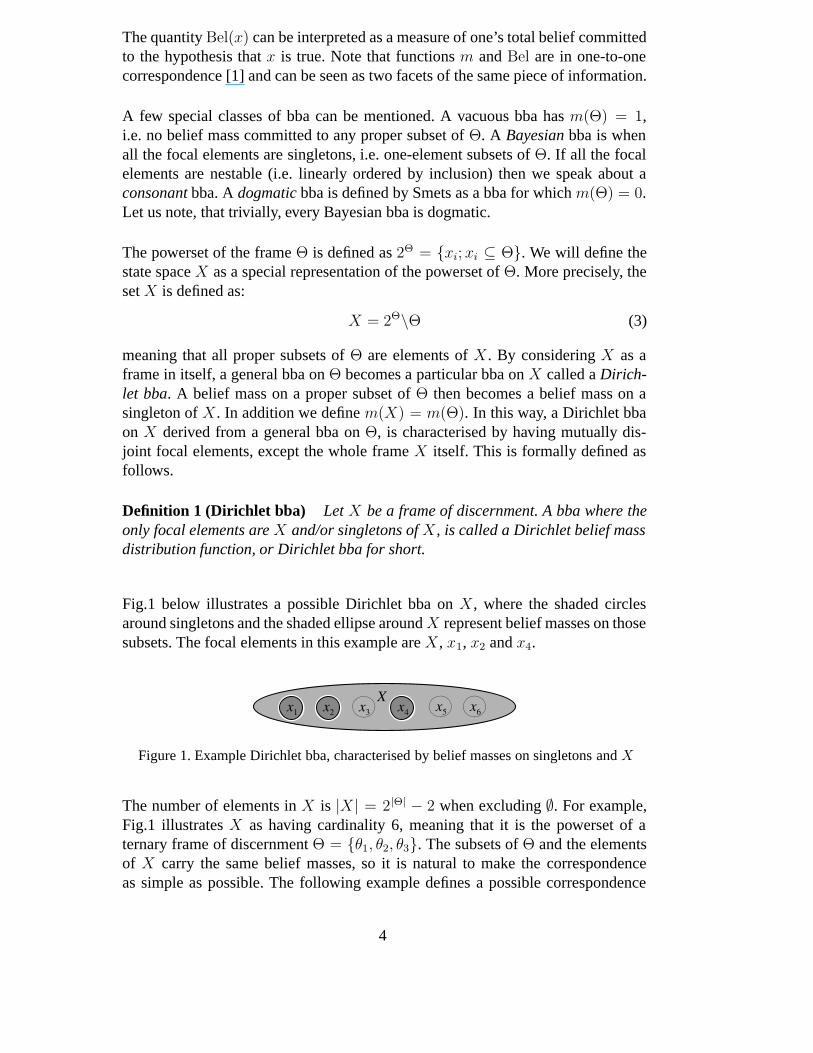
Fig.1 below illustrates a possible Dirichlet bba on X , where the shaded circlesaround singletons and the shaded ellipse around X represent belief masses on thosesubsets. The focal elements in this example are X , x1, x2 and x4.

Figure 1. Example Dirichlet bba, characterised by belief masses on singletons and X

The number of elements in X is |X| = 2|Θ| − 2 when excluding ∅. For example,Fig.1 illustrates X as having cardinality 6, meaning that it is the powerset of aternary frame of discernment Θ = {θ1, θ2, θ3}. The subsets of Θ and the elementsof X carry the same belief masses, so it is natural to make the correspondenceas simple as possible. The following example defines a possible correspondence

4

between subsets of Θ and elements of X:

x1 ←→ θ1, x4 ←→ θ1 ∪ θ2, X ←→ Θ .

x2 ←→ θ2, x5 ←→ θ1 ∪ θ3 ,

x3 ←→ θ3, x6 ←→ θ2 ∪ θ3 ,

(4)

The number of focal elements of a Dirichlet bba on X can be at most |X| + 1,which happens when every element as well as X is a focal element.

The name “Dirichlet” bba is used because bbas of this type are equivalent to Dirich-let probability density functions under a specific mapping. A bijective mapping be-tween Dirichlet bbas and Dirichlet probability density functions is defined in [15],and is also described in Sec.4 below. Our approach is different from that of Walley’sImprecise Dirichlet Model [17] which interprets the situations of frame ignoranceand frame certainty in the Dirichlet model as lower and upper probability in thebelief model.

3 The Dirichlet Multinomial Model

The cumulative and averaging rules of combination, to be described in detail in thefollowing sections, are firmly rooted in the classical Bayesian inference theory, andare equivalent to addition and averaging of multinomial observations respectively.For self-containment, we briefly outline the Dirichlet multinomial model below,and refer to [18] for more details.

3.1 The Dirichlet Distribution

We are interested in knowing the probability distribution over the disjoint elementsof a frame based on observed instances of these elements. In case of binary frames,it is determined by the Beta distribution. In the general case it is determined bythe Dirichlet distribution, which describes the probability distribution over a k-component random variable p(xi), i = 1, . . . k with sample space [0, 1]k, subjectto the additivity criterion:

k∑i=1

p(xi) = 1 . (5)

Note that for any sample from a Dirichlet random variable, it is sufficient to de-termine values for p(xi) for any k − 1 elements i of {1, . . . , k}, as this uniquelydetermines the value of the remaining variable.

5

The Dirichlet distribution with prior captures a sequence of observations of the kpossible outcomes with k positive real observation variables r(xi), i = 1 . . . k,each corresponding to one of the possible outcomes. In order to have a compactnotation we define a vector �p = {p(xi) | 1 ≤ i ≤ k} to denote the k-componentrandom probability variable, and a vector �r = {ri | 1 ≤ i ≤ k} to denote thek-component random observation variable [r(xi)]

ki=1.

In order to distinguish between the a priori information and the a posteriori ev-idence, the Dirichlet distribution must be expressed with prior information repre-sented as a base rate vector �a over the frame as well as the non-informative priorweight C. Eq.(6) represents this Dirichlet Distribution with Prior.

f(�p | �r,�a) =Γ

(k∑

i=1(r(xi) + a(xi)C)

)

k∏i=1

Γ (r(xi) + a(xi)C)

k∏i=1

p(xi)r(xi)+a(xi)C−1 (6)

The vector �p represents first order probability variables over the elements of Xsatisfying Eq.(5), whereas the density f(�p | �r,�a) represents the probability of spe-cific sets of values for the first-order variables. Since the first-order variables �pare continuous, the second-order probability f(�p | �r,�a) for any given value ofp(xi) ∈ [0, 1] is vanishingly small and therefore meaningless as such. It is onlymeaningful to compute

∫ p2p1

f(p(xi) | �r,�a) for a given interval [p1, p2] and state xi,or simply to compute the expectation value of p(xi). As will be shown below, thisprovides a sound mathematical basis for accumulating and averaging evidence.

Given the Dirichlet distribution of Eq.(6), the probability expectation of any of thek random variables can now be written as:

E(p(xi) | �r,�a) = r(xi) + a(xi)C

C +∑k

t=1 r(xt). (7)

Eq.(6) is useful, because it allows the determination of the probability distributionwith arbitrary amounts of observation evidence, even without any observations.

The non-informative prior weight C is set to C = 2 when a uniform distributionover binary frames is assumed. Selecting a larger value for C will result in newobservations having less influence over the Dirichlet distribution. A distribution isnon-informative when it only reflects knowledge of the frame, and does not reflectany observation evidence.

It can be noted that it would be unnatural to require a uniform distribution overarbitrary large frames because it would make the sensitivity to new evidence arbi-trarily small. For example, requiring a uniform a priori distribution over a frame

6

of cardinality 100, would force C = 100. In case an event of interest has beenobserved 100 times, and no other event has been observed, the derived probabilityexpectation of the event of interest will still only be about 1

2, which would seem

totally counter-intuitive. In contrast, when a uniform distribution is assumed in thebinary case, and the same 100 observations are analysed, the derived probabilityexpectation of the event of interest would be close to 1, as intuition would dictate.The value of C determines the approximate number of observations of a particularelement in the frame needed to influence the probability expectation value of thatelement from 0 to 0.5

It can be noted that according to Walley’s IDM (Imprecise Dirichlet Model) [17]the upper and lower probability for a state xi are obtained by setting a(xi) = 1and a(xi) = 0 respectively. The lower probability is thus based on a zero base rate,and the upper probability is based on a base rate equal to one.The upper and lowerprobabilities are then interpreted as the upper and lower bounds for the probabilityof the outcome. While this is an interesting interpretation of the Dirichlet distri-bution, it can not be taken literally. According to this model, the upper and lowerprobability values for an outcome xi are defined as:

IDM Upper probability: P (xi) =r(xi) + C

C +∑k

i=1 r(xi)(8)

IDM Lower probability: P (xi) =r(xi)

C +∑k

i=1 r(xi)(9)

where r(xi) is the number of observations of outcome xi, and C is the weight ofthe non-informative prior probability distribution. It can easily be shown that thesevalues can be misleading. For example, assume an urn containing 9 red balls and 1black ball, meaning that the relative frequencies of red and black balls are p(red) =0.9 and p(black) = 0.1. The a priori weight is set to C = 2. Assume further that anobserver picks one ball which turns out to be black. According to Eq.(9) the lowerprobability is then P (black) = 1

3. It would be incorrect to literally interpret this

value as the lower bound for the relative frequency because it obviously is greaterthan the actual relative frequency of black balls. This example shows that there isno guarantee that the actual probability of an event is inside the interval defined bythe upper and lower probabilities as described by the IDM. The terms “upper” and“lower” must therefore be interpreted as rough terms for imprecision, and not asabsolute bounds.

The traditional approach in Bayesian analysis is to interpret the combination ofthe base rate vector �a and the a priori weight C as representing specific a prioriinformation such as provided by a domain expert.

7

3.2 Visualising Dirichlet Distributions

Visualising Dirichlet distributions is challenging because it is a density functionover k − 1 dimensions, where k is the frame cardinality. For this reason, Dirichletdistributions over ternary frames are the largest that can be easily visualised onpaper.

With k = 3, the probability distribution has 2 degrees of freedom, and the additivityequation p(x1) + p(x2) + p(x3) = 1, which is an instantiation of Eq.(5), defines atriangular plane as illustrated in Fig.2.

00.2

0.40.6

0.81

00.2

0.40.6

0.81

0

0.2

0.4

0.6

0.8

1

p(x1)p(x2)

p(x3)

Figure 2. Triangular plane

In order to visualise probability density over the triangular plane, it is convenientto lay the triangular plane horizontally in the X:Y-plane, and visualise the densitydimension along the Z-axis.

Let us consider the example of an urn containing balls that can have the inscriptionx1, x2 or x3 (i.e. k = 3). Let us first assume that no other information than thecardinality of the frame is available, meaning that r(x1) = r(x2) = r(x3) = 0, anda(x1) = a(x2) = a(x3) = 1/3. Then Eq.(7) dictates that the expected probabilityof picking a ball of any type is equal to the base rate probability, which is 1

3. The a

priori Dirichlet density function is illustrated in Fig.3.a.

Let us now assume that an observer has picked x1 6 times, x2 once and x3 once, i.e.r(x1) = 6, r(x2) = 1, r(x3) = 1. By assuming a prior weight C = 2 as before,the a posteriori expected probability of picking a ball with x1 can be computed asE(p(x1)) =

23. The a posteriori Dirichlet density function is illustrated in Fig.3.b.

We reuse the example of the urn containing balls with the inscriptions x1, x2, andx3, but this time we assume a binary partition of X into {x1, x1}, i.e. where x1 =x2 ∪ x3. The base rate of picking a ball with inscription x1 is set to a(x1) =

13

asbefore because the urn still contains balls of three different types, and the groupingof states x2 and x3 is purely technical.

Let us again assume that an observer has picked (with return) x1 6 times, and

8

0

5

10

15

20

1

0

1

0

1

0

.

p(x1)p(x2)

p(x3)

Densityf(�p | �r,�a)

(a) Prior Dirichlet distribution

0

5

10

15

20

1

0

1

0

1

0

.

p(x1)p(x2)

p(x3)

Densityf(�p | �r,�a)

(b) Posterior Dirichlet distribution

Figure 3. Visualising a priori and a posteriori Dirichlet distributions

{x2 or x3} twice, i.e. r(x1) = 6 and r(x1) = 2.

Since the frame has been reduced to binary, the Dirichlet distribution is reducedto a Beta distribution which is simple to visualise. The a priori and a posterioridensity functions are illustrated in Fig.3.2.

0

1

2

3

4

5

6

7

0 0.2 0.4 0.6 0.8 1

Den

sity

.

p(x1)(a) Prior Beta distribution

0

1

2

3

4

5

6

7

0 0.2 0.4 0.6 0.8 1

Den

sity

.

p(x1)(b) Posterior Beta distribution

Figure 4. Visualising prior and posterior Beta distributions

The a posteriori expected probability of picking a ball with inscription x1 can becomputed with Eq.(7) as E(p(x1)) = 2

3, which is the same as before the coarsen-

ing, as illustrated in Fig.3.b This shows that the coarsening does not influence theprobability expectation value of specific events.

4 Mapping Between Dirichlet Distribution and Belief Distribution Functions

In this section we will define a bijective mapping between Dirichlet probabilitydistributions described in Sec.3, and Dirichlet bbas described in Sec.2.

9

Let X = {xi; i = 1, · · ·k} be a frame where each singleton represents a possibleoutcome of a state variable. It is assumed that X represents the powerset of a frameof discernment Θ according to Eq.(eq:powerset). Let m be a general bba on Θ andtherefore a Dirichlet bba on X , and let f(�p | �r,�a) be a Dirichlet distribution overX .

The bijective mapping between m and f(�p | �r,�a) is based on simple intuitivecriteria specified below. The mathematical expressions for the bijective mappingcan be directly derived from the criteria.

As first criterion we require equality between the pignistic probability values ℘(xi)derived from m, and the probability expectation values E(p(xi)) of f(�p | �r,�a). Forall xi ∈ X , this constraint is expressed as:

℘(xi) = E(p(xi) | �r,�a) ⇐⇒ m(xi) + a(xi)m(X) =r(xi) + a(xi)C

C +∑k

t=1 r(xt)(10)

We also require m(xi) to be an increasing function of r(xi), and m(X) to be adecreasing function of

∑kt=1 r(xt). In other words, the more evidence in favour of

a particular outcome, the greater its belief mass. Furthermore, the less evidenceavailable in general, the more vacuous the bba (i.e. the greater m(X)). These in-tuitive requirements together with Eq.(10) imply the bijective mapping defined byEq.(11).

For m(X) �= 0 :⎧⎪⎪⎪⎪⎪⎪⎨⎪⎪⎪⎪⎪⎪⎩

m(xi) = r(xi)

C +∑k

t=1r(xt)

m(X) = C

C +∑k

t=1r(xt)

⇐⇒

⎧⎪⎪⎪⎪⎪⎨⎪⎪⎪⎪⎪⎩

r(xi) =Cm(xi)m(X)

1 = m(X) +∑k

i=1m(xi)

(11)

Next we consider the case of zero uncertainty. In case m(X) −→ 0, then necessar-ily

∑ki=1m(xi) −→ 1, and

∑ki=1 r(xi) −→ ∞, meaning that at least some, but not

necessarily all, of the evidence parameters r(xi) are infinite.

We define η(xi) as the the relative degree of infinity between the corresponding in-finite evidence parameters r(xi) such that

∑ki=1 η(xi) = 1. When infinite evidence

parameters exist, any finite evidence parameter r(xi) can be assumed to be zero inany practical situation because it will have η(xi) = 0, i.e. it will carry zero weightrelative to the infinite evidence parameters. This leads to the bijective mapping de-fined by Eq.(12).

10

For m(X) = 0 :⎧⎪⎪⎪⎪⎪⎨⎪⎪⎪⎪⎪⎩

m(xi) = η(xi)

m(X) = 0

⇐⇒

⎧⎪⎪⎪⎪⎪⎪⎨⎪⎪⎪⎪⎪⎪⎩

r(xi) = η(xi)k∑

t=1r(xt) = η(xi)∞

1 =k∑

t=1m(xt)

(12)

In case η(xi) = 1 for a particular evidence parameter r(xi), then r(xi) = ∞ andall the other evidence parameters are finite. In case η(xi) = 1/l for all i = 1 . . . l,then all the evidence parameters are all equally infinite.

5 Deriving the Cumulative Rule of Belief Fusion

The cumulative rule is equivalent to a posteriori updating of Dirichlet distributions,and is based on the bijective mapping described in the previous section.

Assume a process with possible outcomes defined by the frame of discernment Θ.Let X = {xi; i = 1, · · ·k} represent the powerset of Θ according to Eq.(3). Letagents A and B observe the outcomes of the process over two separate time periods,assuming that they apply the same base rate vector �a to Θ. Let the two observers’respective observations be expressed as �rA and �rB . The Dirichlet distributions re-sulting from these separate bodies of evidence can be expressed as f(�p | �rA,�a) andf(�p | �rB,�a)

The fusion of these two bodies of evidence simply consists of vector addition of �rAand �rB. In terms of Dirichlet distributions, this can be expressed as:

f(�p | �rA�B,�a) = f(�p | �rA,�a) ⊕ f(�p | �rB,�a)= f(�p | (�rA + �rB),�a) .

(13)

The symbol “�” denotes the cumulative fusion of two observers A and B into asingle imaginary observer denoted as A �B. All the necessary elements are now inplace for presenting the cumulative rule for belief fusion.

Theorem 1 (Cumulative Fusion Rule)Let mA and mB be bbas respectively held by agentsA and B over the same frame ofdiscernment Θ. Let X = {xi; i = 1, · · ·k} represent the powerset of Θ accordingto Eq.(3). Let mA�B be the bba such that:

11

Case I: For (mA(Θ) �= 0) ∨ (mB(Θ) �= 0) :⎧⎪⎪⎪⎪⎪⎨⎪⎪⎪⎪⎪⎩

mA�B(xi) =mA(xi)mB(Θ)+mB(xi)mA(Θ)mA(Θ)+mB(Θ)−mA(Θ)mB(Θ)

mA�B(Θ) = mA(Θ)mB(Θ)mA(Θ)+mB(Θ)−mA(Θ)mB(Θ)

(14)

Case II: For (mA(Θ) = 0) ∧ (mB(Θ) = 0) :⎧⎪⎪⎪⎪⎪⎨⎪⎪⎪⎪⎪⎩

mA�B(xi)= γAmA(xi) + γBmB(xi)

mA�B(Θ)= 0

where

⎧⎪⎪⎪⎪⎪⎨⎪⎪⎪⎪⎪⎩

γA= limmA(Θ)→0mB(Θ)→0

mB(Θ)mA(Θ)+mB(Θ)

γB= limmA(Θ)→0mB(Θ)→0

mA(Θ)mA(Θ)+mB(Θ)

(15)

Then mA�B is called the cumulatively fused bba of mA and mB , representing animaginary agent [A �B]’s bba, as if that agent represented both A and B. By usingthe symbol ‘⊕’ to designate this belief operator, we define mA�B ≡ mA ⊕mB .

In Case II, γA and γB are relative weights satisfying γA + γB = 1. The defaultvalues are γA = γB = 0.5.

The proof below provides details about how the expression for the cumulative ruleis derived.

Proof 1 Let mA and mB be Dirichlet bbas. The mapping from Dirichlet bbas toDirichlet distributions is done according to the right hand sides of Eq.(11) andEq.(12), expressed as:

mA �−→ f(�p | �rA,�a)mB �−→ f(�p | �rB,�a)

(16)

These Dirichlet distributions can now be fused according to Eq.(13), expressed as:

f(�p | �rA,�a)⊕ f(�p | �rB,�a) = f(�p | (�rA + �rB),�a) (17)

Finally, the result of Eq.(17) is mapped back to a (cluster) Dirichlet bba again usingEq.(11). This can be written as:

f(�p | (�rA + �rB),�a) �−→ mA�B (18)

By inserting the full expressions for the parameters in Eqs.(16), (17) and (18), theexpressions of Eqs.(14) and (15) in Theorem 1 emerge.

�

12

It can be verified that the cumulative rule is commutative, associative and non-idempotent. The non-idempotence means that cumulative fusion of two equal ar-gument bbas will result in a different bba. In Case II of Theorem 1 (Bayesian bbas,which can also be described as dogmatic Dirichlet bbas), the associativity dependson the preservation of relative weights of intermediate results, which requires theadditional weight variable γ. In this case, the cumulative rule is equivalent to theweighted average of probabilities.

It is interesting to notice that the expression for the cumulative rule is independentof the a priori weight C. That means that the choice of a uniform Dirichlet dis-tribution in the binary case in fact only influences the mapping between Dirichletdistributions and Dirichlet bbas, not the cumulative rule itself. This shows that thecumulative rule is firmly based on classical statistical analysis, and not dependenton arbitrary choices of prior.

The cumulative fusion operator for opinions 2 in subjective logic [5,12,16] is a spe-cial case of the cumulative belief fusion rule, and emerges directly from Theorem 1by assuming a Dirichlet bba on the frame.

6 Deriving the Averaging Rule of Belief Fusion

The averaging rule is equivalent to averaging the evidence of Dirichlet distributions,and is based on the bijective mapping between the belief and evidence notationsdescribed in Sec.4.

Assume a process with possible outcomes defined by the frame of discernmentΘ. Let X = {xi; i = 1, · · ·k} represent the powerset of Θ according to Eq.(3).Let two sensors A and B observe the same outcomes of the process, i.e. over thesame time period, assuming that they apply the same base rate vector �a to Θ. Letthe two sensors’ respective observations be expressed as �rA and �rB. The Dirichletdistributions resulting from these separate bodies of evidence can be expressed asf(�p | �rA,�a) and f(�p | �rB,�a)

The averaging fusion of these two bodies of evidence simply consists of the averagevector value of �rA and �rB . In terms of Dirichlet distributions, this is expressed as:

f(�p | �rA�B,�a) = f(�p | �rA,�a) ⊕ f(�p | �rB,�a)= f(�p | (�rA+�rB

2),�a) .

(19)

2 In the binomial case also called the consensus operator.

13

The symbol “�” denotes the averaging fusion of two observers A and B into asingle imaginary observer denoted as A�B.

Theorem 2 Averaging Fusion Rule

Let mA and mB be bbas respectively held by agents A and B over the same frameΘ. Let X = {xi; i = 1, · · ·k} represent the powerset of Θ according to Eq.(3). LetmA�B be the bba such that:

Case I: For (mA(Θ) �= 0) ∨ (mB(Θ) �= 0) :⎧⎪⎪⎪⎪⎪⎨⎪⎪⎪⎪⎪⎩

mA�B(xi) =mA(xi)mB(Θ)+mB(xi)mA(Θ)

mA(Θ)+mB(Θ)

mA�B(Θ) = 2mA(Θ)mB(Θ)mA(Θ)+mB(Θ)

(20)

Case II: For (mA(Θ) = 0) ∧ (mB(Θ) = 0) :⎧⎪⎪⎪⎪⎪⎨⎪⎪⎪⎪⎪⎩

mA�B(xi)= γAmA(xi) + γBmB(xi)

mA�B(Θ)= 0

where

⎧⎪⎪⎪⎪⎪⎨⎪⎪⎪⎪⎪⎩

γA= limmA(Θ)→0mB(Θ)→0

mB(Θ)mA(Θ)+mB(Θ)

γB= limmA(Θ)→0mB(Θ)→0

mA(Θ)mA(Θ)+mB(Θ)

(21)

Then mA�B is called the averaged bba of mA and mB , representing the averagingfusion of the bbas of A and B. By using the symbol ‘⊕’ to designate this beliefoperator, we define mA�B ≡ mA⊕mB .

It can be verified that the averaging fusion rule is commutative, and idempotent,but not associative. The non-associativity means that averaging fusion of three ar-gument bbas will produce different results depending on which two bbas are fusedfirst. The averaging rule represents a generalisation of the averaging fusion operatorfor opinions 3 in subjetive logic[12,13].

In Case II, γA and γB are relative weights satisfying γA + γB = 1. The defaultvalues are γA = γB = 0.5.

The proof below provides details about how the expression for the averaging ruleis derived.

Proof 2 Let mA and mB be Dirichlet bbas. The mapping from Dirichlet bbas toDirichlet distributions is done according to the right hand sides of Eq.(11) and

3 In the binomial case also called the consensus operator for dependent opinions.

14

Eq.(12), expressed as:

mA �−→ f(�p | �rA,�a)mB �−→ f(�p | �rB,�a)

(22)

The average of these Dirichlet distributions can now be obtained according toEq.(19), expressed as:

f(�p | �rA,�a)⊕f(�p | �rB,�a) = f(�p | (�rA+�rB2

),�a) (23)

Finally, the result of Eq.(23) is mapped back to a Dirichlet bba again using Eq.(11).This can be written as:

f(�p | (�rA + �rB2

),�a) �−→ mA�B (24)

By inserting the full expressions for the parameters in Eqs.(22), (23) and (24), theexpressions of Eqs.(20) and (21) in Theorem 2 emerge.

�

7 Examples

In this section, we will illustrate by examples the results of applying the cumulativeand averaging rules, as well as Dempster’s rule of fusing beliefs. Each example ischosen to illustrate that it is crucial to select the appropriate rule for modelling aspecific situation.

To make the presentation self contained, we also include the definitions of Con-junctive Rule and of Dempster’s Rule below:

Definition 2 (The Conjunctive Rule) .

[mA ∩©mB](x) =∑

y∩z=x

mA(y)mB(z) ∀ x ⊆ X. (25)

This rule is referred to as the conjunctive rule of combination, or the non-normalisedDempster’s rule. If necessary, the normality assumption m(∅) = 0 can be recoveredby dividing each mass by a normalisation coefficient. The resulting operator knownas Dempster’s rule is defined as:

Definition 3 (Dempster’s Rule) .

[mA �mB](x) =[mA ∩©mB](x)

1− [mA ∩©mB](∅) ∀ x ⊆ X, x �= ∅ (26)

15

The use of Dempster’s rule is possible only if mA and mB are not totally conflicting,i.e., if there exist two focal elements y and z of mA and mB satisfying y ∩ z �= ∅.

7.1 Zadeh’s Example

This well known example was put forward by Zadeh [19] to show that Dempster’srule can produce counter-intuitive results when applied to particular situations.

The averaging rule produces results well in line with intuition when applied to thisexample, as will be shown below.

Suppose that we have a murder case with three suspects; Peter, Paul and Mary,and two witnesses WA and WB who give highly conflicting testimonies. The ex-ample assumes that the most reasonable conclusion about the likely murderer canbe obtained by fusing the beliefs expressed by the two witnesses. Table 1 gives thewitnesses’ belief masses in the case of Zadeh’s example and the resulting beliefmasses after applying Dempster’s rule. The abbreviations “CR”, “AR” and “DR”stand for Cumulative Rule, Averaging Rule, and Dempster’s Rule respectively.

WA WB CR AR DR

m(Peter) = 0.99 0.00 0.495 0.495 0.00

m(Paul) = 0.01 0.01 0.010 0.010 1.00

m(Mary) = 0.00 0.99 0.495 0.495 0.00

m(Θ) = 0.00 0.00 0.000 0.000 0.00Table 1Zadeh’s example (averaging situation)

In case of Bayesian bbas such as in Zadeh’s example, the cumulative rule and theaveraging rules are equivalent, and represent the weighted average of probabilities.

The question now arises whether Zadeh’s example represents a cumulative, an av-eraging or a conjunctive situation. Said differently, in case the testimonies can beconsidered as statistical evidence which is accumulated during the trial, then the cu-mulative rule should be applied. In case the testimonies should be weighted againsteach other to produce a balanced opinion, then the averaging rule should be ap-plied. In case the testimonies can be considered as two different logical statementsthat are to be conjunctively combined as a function of their respective belief values,then Dempster’s rule should be applied. In our view, an adequate model for thecourt case in Zadeh’s example should reflect how a judge or a jury would weighthe testimonies against each other, which implies that the averaging rule is the bestalternative.

16

7.2 Zadeh’s Example Modified

Fusion of highly conflicting beliefs is problematic when applying Dempster’s ruleas in the original Zadeh’s example. Many authors [20] explain this by saying thatproblem to certain degree can be remedied by discounting the testimonies beforebeing fused, in order to reduce their degree of conflict. This approach is illustratedby the Modified Zadeh’s example [21] below.

By introducing a small amount of uncertainty in the witnesses testimonies (seeTable 2), the cumulative and averaging rules produce different but still very similarresults. Dempster’s Rule now produces almost the same results as the cumulativeand averaging rules, but which are very different from those it produced in theoriginal Zadeh’s Example.

WA WB CR AR DR

m(Peter) = 0.98 0.00 0.4925 0.4900 0.4900

m(Paul) = 0.01 0.01 0.0100 0.0100 0.0150

m(Mary) = 0.00 0.98 0.4925 0.4900 0.4900

m(Θ) = 0.01 0.01 0.0050 0.0100 0.0050Table 2Modified Zadeh’s example (averaging situation)

The introduction of a small amount of ignorance in the bbas was sufficient to makeDempster’s rule produce intuitive results. Although it can be argued that witnesstestimonies should always be considered with a degree of uncertainty, it is prob-lematic that Dempster’s rule breaks down when the argument bbas are certain as inthe case of Zadeh’s original example. The discontinuity of the results demonstratesthat Dempster’s rule is inappropriate in this situation. The correct model for boththe original and the modified Zadeh’s example is the averaging rule because it doesnot produces any discontinuity between the two situations, and because testimoniesof witnesses having observed the same murder should be considered as dependentstatistical evidence.

7.3 Fusing Independent Sensor Evidence

This example will illustrate the fusion of cumulative evidence.

Assume that a GE (Genetical Engineering) process can produce fish eggs that areeither Male (M) or Female (F), and that two sensors observe whether Male andFemale eggs are produced. For the purpose of independence it is here assumed thatthe sensors observe the processes at different time periods, which means that noneof the eggs observed by the first sensor are also observed by the second sensor. The

17

frame has two elements: Θ = {M, F} and so does the corresponding powerset Xwhich can be expressed as X = 2Θ\Θ = {M, F}.

Assume that the observations by the two sensors produce equal and non-conflictingbeliefs as given in the Table 3 below over the two time periods:

SA SB CR AR DR

m(M) = 0.99 0.99 0.994975 0.99 0.9999

m(F) = 0.00 0.00 0.00 0.00 0.00

m(Θ) = 0.01 0.01 0.005025 0.01 0.0001Table 3Fusion of independent beliefs from two sensors (cumulative situation)

Applying the cumulative rule and Dempster’s rule to these beliefs results in a reduc-tion in uncertainty, and a convergence towards the largest belief mass of the sensoroutputs. Applying the averaging rule preserves the values of the input observationbbas, because both are equal.

Intuitively, fusion should reduce the ignorance because more evidence is taken intoaccount in this situation. The averaging rule can therefore be dismissed because itdoes not reduce the ignorance.

In case of the cumulative rule, the input beliefs are equivalent to each sensor havingobserved 198 Male eggs (r(M) = 198), and no Female eggs (r(F) = 0), with theuncertainty computed as mA�B(Θ) = 2/(r(M) + r(F) + 2) = 0.01. The outputbeliefs is equivalent to the observation of 2r(M) = 396 Male eggs, with the uncer-tainty computed as m(Θ) = 2/(396 + 2) = 0.005025. The output uncertainty ofthe cumulative rule is thus halved, which is what one would expect in the case ofcumulative fusion.

In case of Dempster’s rule, the uncertainty is reduced to the product of the inputuncertainties computed as:

[mA �mB](Θ) = mA(Θ)mB(Θ) = 0.0001 (27)

i.e. by a factor of 1/100 which represents a very fast convergence. In fact, whenconsidering that the amount of evidence has only been doubled, a reduction inuncertainty by a factor of 1/100 is too fast when considering this as a cumulativesituation. When fusing two equal sensor outputs, one should expect the uncertaintyto be reduced by 1/2, because the double amount of observations have been made.

The difference in convergence i.e. the rate of uncertainty reduction, is noteworthy,and clearly illustrates that Dempster’s rule in fact is not applicable to this situation,even in the case of non-conflicting beliefs. This is because the example describes acumulative situation, and that it would be meaningless to model it with a conjunc-tive fusion rule.

18

7.4 Conjunctive Fusion of Beliefs

In this example we consider the case of a loaded dice, where Θ = {1, 2, 3, 4, 5, 6} isthe set of possible outcomes. An informant has special knowledge about the loadeddice, and an observer is trying to predict the outcome of throwing the dice based onhints from the informant.

First the informant provides hint A which says that the dice will always produce aneven number. The observer translates this into the belief mass mA({2, 4, 6}) = 1.Then the informant provides hint B which says that the dice will always produce aprime number. The observer translates this into the belief mass mB({2, 3, 5}) = 1.

Table 4 shows the results of applying the cumulative, averaging and Dempster’srule to these bbas.

mA mB CR AR DR

m({2, 4, 6}) = 1.00 0.00 0.50 0.50 0.00

m({2, 3, 5}) = 0.00 1.00 0.50 0.50 0.00

m({2}) = 0.00 0.00 0.00 0.00 1.00

m(Θ) = 0.00 0.00 0.00 0.00 0.00Table 4Fusion of hints about loaded dice (conjunctive situation)

The two hints are sufficient to determine that {2} is the only possible outcome. Thisresult is obtained by conjunctive combination of the input evidence, as dictated byDempster’s rule. The conjunctive approach of DR is appropriate in this situationbecause the input evidence applies to different and orthogonal focal sets, whichwould make it problematic to apply either the cumulative or averaging rules.

The correct answer could be obtained by applying a normalised version of the cu-mulative rule [22], but this approach should be considered as ad-hoc. The situationis clearly conjunctive in nature, which means that Dempster’s rule or the conjunc-tive rule is appropriate.

8 Discussion

The cumulative and averaging rules of belief fusion make it possible to use the the-ory of belief functions for modelling situations where evidence is combined in acumulative or averaging fashion. Such situations could previously not be correctlymodelled within the framework of belief theory. It is worth noticing that the cumu-lative, averaging rules and Dempster’s rule apply to different types of belief fusion,

19

and that, strictly speaking, is meaningless to compare their performance in the sameexamples. The notion of cumulative and averaging belief fusion as opposed to con-junctive belief fusion has therefore been introduced in order to make this distinctionexplicit.

There is however considerable confusion regarding the applicability of Dempster’srule, which e.g. is illustrated by applying Dempster’s rule to the court case situationin Zadeh’s example. Often the problem is to identify which model best fits a partic-ular situation. The court case of Zadeh’s example intuitively requires an averagingapproach, the fusion of independent evidence from sensors that measure the samephenomenon intuitively requires a cumulative approach, and logical conjunction ofevidence intuitively requires a conjunctive approach as through Dempster’s rule.

To be more specific about the applicability of Dempster’s rule, the two bbas tobe fused are required to be orthogonal. Being orthogonal means that the bbas areobtained by deliberately considering different subsets of the frame. This is for ex-ample the case in the application of Dempster’s rule in the framework of Kohlas’theory of hints [23]. In the example of the loaded dice from Sec.7.4, the informantdeliberately provides only a part of the truth when giving the hints, and each hintfocuses on a specific subset.

The following scenario will illustrate using the cumulative and the averaging fu-sion rules, as well as Dempster’s rule. Assume again that GE process can produceMale (M) or Female (F) eggs, and that in addition, each egg can have geneticalmutation 1 or 2 independently of its gender. This constitutes the quaternary frameΘ = {M1,M2,F1,F2}. Sensors IA and IB simultaneously observe whether eachegg is M or F, and Sensor II observes whether the egg has mutation 1 or 2.

Assume that Sensors IA and IB have derived two separate bbas regarding the genderof a specific egg, and that Sensor II has produced a bba regarding its mutation.Because Sensors IA and IB have observed the same aspect simultaneously, thebbas should be fused with the averaging rule. Sensor II has observed a differentand orthogonal aspect, so the output of the AR fusion and the bba of Sensor IIshould be combined with Dempster’s Rule. This is illustrated in Fig.5.

This result from fusing the two orthogonal beliefs with Dempster’s Rule can nowbe considered as a single observation. By combining beliefs from multiple obser-vations it is possible to express the most likely status of future eggs as a predictivebelief. We are now dealing with two different situations which must be consideredseparately. The first situation relates to the state of a given egg that the sensors havealready observed. The second situation relates to the possible state of eggs that willbe produced in the future. A bba in the first situation is based on the sensors asillustrated inside Observation 1 in Fig.5. The second situation relates to combiningmultiple observations, as illustrated by fusing the beliefs from Observation 1 andObservation 2 in Fig.5.

20

Figure 5. Applying different types of belief fusion according to the situation

In order to fuse observations, the bba for each observation must be normalised tocarry the weight corresponding to a single Bayesian observation. This is done bymultiplying all belief masses on proper subsets of Θ with the factor λ expressed as:

λ =m(Θ) + C(1−m(Θ))

2C(28)

The belief mass on Θ is then increased to compensate for the decreased beliefmasses on the proper subsets of Θ. This produces the normalised bba:

m′ :

⎧⎪⎨⎪⎩m(x′

i) = λm(xi)

m′(Θ) = m(Θ) + (1− λ)(1−m(Θ)(29)

Table 5 provides a numerical example that relates directly to the situations of Fig.5.Table entries with zero value are omitted. For simplicity it is assumed that Obser-vation 2 produces the same beliefs as observation 1.

From Table 5 it can be seen that most likely egg in Observation 1 is Male withmutation 1, which is supported with belief mass b(M1) = 0.7.

To proceed from the results of DR to the values of Obs.1, the computation of thenormalisation factor λ is required. By using Eq.(28) and setting C = 2 we get λ =0.498125. By using Eq.(29) the values in the column of Obs.1 can be computed,which represents the predictive bba resulting from one observation. For simplicitythe bba of Obs.2 is set identical to that of Obs.1. It is then possible to fuse the twoobservations with the cumulative rule, as expressed by the rightmost column, to geta more accurate predictive bba of future observations.

It can be observed that the application of Dempster’s rule in the examples abovedid not require any normalisation. In that case Dempster’s rule is equivalent to theconjunctive rule of Def.2 could have been used.

21

SIA SIB AR SII DR Obs.1 Obs.2 CR

m({M1,M2}) 0.90 0.80 0.875 0.0875 0.0436 id. 0.0583

m({F1,F2}) 0.05 0.05 0.050 0.0050 0.0025 id. 0.0033

m({M1,F1}) 0.80 0.0600 0.0299 id. 0.0400

m({M2,F2}) 0.10 0.0075 0.0037 id. 0.0050

m({M1}) 0.7000 0.3487 id. 0.4667

m({M2}) 0.0875 0.0436 id. 0.0583

m({F1}) 0.0400 0.0199 id. 0.0267

m({F2}) 0.0050 0.0025 id. 0.0033

m(Θ) 0.05 0.15 0.075 0.10 0.0075 0.5056 id. 0.3384Table 5Application of different types of belief fusion according to the situations in Fig.5

9 Conclusion

Different situations require different types of belief fusion. We have described thecumulative and the averaging belief fusion rules which can be used for belief fusionin situations where Dempster’s rule is inadequate. The two new rules represent gen-eralisations of the corresponding fusion operators for opinions used in subjectivelogic, and have been derived from classical Bayesian analysis through a bijectivemapping between Dirichlet distributions and belief functions.

This simple mapping positions belief theory and statistical theory closely and firmlytogether. This is important in order to make belief theory more practical and easierto interpret, and to make belief theory more acceptable in the main stream statisticsand probability communities.

References

[1] G. Shafer, A Mathematical Theory of Evidence. Princeton University Press, 1976.

[2] M. Daniel, “Associativity in combination of belief functions,” in Proceedings of 5thWorkshop on Uncertainty Processing. - Praha, Edicni oddeleni VSE 2000. Springer,2000, pp. 41–54.

[3] J. Dezert, “Foundations for a new theory of plausible and paradoxical reasoning,”Information & Security Journal, vol. 9, 2002.

[4] D. Dubois and H. Prade, “Representation and combination of uncertainty with belieffunctions and possibility measures,” Comput. Intell., vol. 4, pp. 244–264, 1988.

22

[5] A. Jøsang, “The Consensus Operator for Combining Beliefs,” Artificial IntelligenceJournal, vol. 142, no. 1–2, pp. 157–170, October 2002.

[6] E. Lefevre, O. Colot, and P. Vannoorenberghe, “Belief functions combination andconflict management,” Information Fusion, vol. 3, no. 2, pp. 149–162, June 2002.

[7] C. K. Murphy, “Combining belief functions when evidence conflicts,” DecisionSupport Systems, vol. 29, pp. 1–9, 2000.

[8] P. Smets, “The combination of evidence in the transferable belief model,” IEEETransansactions on Pattern Analysis and Machine Intelligence, vol. 12, no. 5, pp. 447–458, 1990.

[9] R. Yager, “On the Dempster-Shafer framework and new combination rules,”Information Sciences, vol. 41, pp. 93–137, 1987.

[10] F. Smarandache, “An In-Depth Look at Information Fusion Rules & the Unification ofFusion Theories,” Computing Research Repository (CoRR), Cornell University arXiv,vol. cs.OH/0410033, 2004.

[11] A. Jøsang and S. Pope, “Dempster’s Rule as Seen by Little ColouredBalls,” (submitted to) Computational Intelligence Journal, 2010, available fromhttp://persons.unik.no/josang/.

[12] A. Jøsang, S. Pope, and S. Marsh, “Exploring Different Types of Trust Propagation,” inProceedings of the 4th International Conference on Trust Management (iTrust), Pisa,May 2006.

[13] A. Jøsang, “Probabilistic Logic Under Uncertainty,” in The Proceedings ofComputing: The Australian Theory Symposium (CATS2007), CRPIT Volume 65,Ballarat, Australia, January 2007.

[14] ——, “Cumulative and Averaging Unfusion of Beliefs.” in The Proceedings of theInternational Conference on Information Processing and Management of Uncertainty(IPMU2008), Malaga, June 2008.

[15] A. Jøsang and Z. Elouedi, “Interpreting Belief Functions as Dirichlet Distributions,”in The Proceedings of the 9th European Conference on Symbolic and QuantitativeApproaches to Reasoning with Uncertainty (ECSQARU), Hammamet, Tunisia,November 2007.

[16] A. Jøsang, “A Logic for Uncertain Probabilities,” International Journal ofUncertainty, Fuzziness and Knowledge-Based Systems, vol. 9, no. 3, pp. 279–311,June 2001.

[17] P. Walley, “Inferences from Multinomial Data: Learning about a Bag of Marbles,”Journal of the Royal Statistical Society, vol. 58, no. 1, pp. 3–57, 1996.

[18] A. Gelman et al., Bayesian Data Analysis, 2nd ed. Florida, USA: Chapman andHall/CRC, 2004.

[19] L. Zadeh, “Review of Shafer’s A Mathematical Theory of Evidence,” AI Magazine,vol. 5, pp. 81–83, 1984.

23

[20] R. Haenni, “Shedding New Light on Zadeh’s Criticism of Dempster’s Rule ofCombination,” in Proceedings of Information Fusion, Philadelphia, July 2005.

[21] A. Jøsang, M. Daniel, and P. Vannoorenberghe, “Strategies for Combining ConflictingDogmatic Beliefs,” in Proceedings of the 6th International Conference on InformationFusion, X. Wang, Ed., 2003.

[22] A. Jøsang and S. Pope, “Normalising the Consensus Operator for Belief Fusion,”in Proceedings of the International Conference on Information Processing andManagement of Uncertainty (IPMU2006), Paris, July 2006.

[23] J. Kohlas and P. Monney, A Mathematical Theory of Hints. An Approach to Dempster-Shafer Theory of Evidence, ser. Lecture Notes in Economics and MathematicalSystems. Springer-Verlag, 1995, vol. 425.

24