Constraints manuscript No.(will be inserted by the editor)

Explaining the cumulative propagator?

Andreas Schutt · Thibaut Feydy · Peter J.

Stuckey · Mark G. Wallace

Received: date / Accepted: date

Abstract The global cumulative constraint was proposed for modelling cumulative

resources in scheduling problems for finite domain (FD) propagation. Since that time

a great deal of research has investigated new stronger and faster filtering techniques

for cumulative, but still most of these techniques only pay off in limited cases or are

not scalable. Recently, the “lazy clause generation” hybrid solving approach has been

devised which allows a finite domain propagation engine possible to take advantage

of advanced SAT technology, by “lazily” creating a SAT model of an FD problem as

computation progresses. This allows the solver to make use of SAT explanation and

autonomous search capabilities. In this article we show how, once we use lazy clause

generation, modelling the cumulative constraint by decomposition creates a highly

competitive version of cumulative. Using decomposition into component parts auto-

matically makes the propagator incremental and able to explain itself. We then show

how, using the insights from the behaviour of the decomposition, we can create global

cumulative constraints that explain their propagation. We compare these approaches

to explaining the cumulative constraint on resource constrained project scheduling

problems. All our methods are able to close a substantial number of open problems

from the well-established PSPlib benchmark library of resource-constrained project

scheduling problems.

Keywords Cumulative constraint · Explanations · Nogood learning · Lazy clause

generation · Resource-constrained Project Scheduling Problem

? A preliminary version of this paper appears as [34].

A. Schutt, T. Feydy, and P. J. StuckeyNational ICT Australia, Department of Computer Science & Software Engineering, The Uni-versity of Melbourne, Victoria 3010, AustraliaTel.: +61-3-83441300Fax: +61-3-93481184E-mail: aschutt,tfeydy,pjs@csse.unimelb.edu.au

M. G. WallaceSchool of Computer Science & Software Engineering, Monash University, Clayton, Vic 3800,AustraliaTel.: +61-3-99051367Fax: +61-3-99031077E-mail: mark.wallace@infotech.monash.edu.au

2

f

d

c

e

ba

source sink

0 2

ab

4 6 8 10 12 14

cde

f

16 18 20

Fig. 1 (a) A small cumulative resource problem, with 6 tasks to place in the 5x20 box, withtask a before b before c, and task d before e (b) a possible schedule..

1 Introduction

Cumulative resources are part of many real-world scheduling problems. A resource can

represent not only a machine which is able to run multiple tasks in parallel but also

entities such as: electricity, water, consumables or even human skills. Those resources

arise for example in the resource-constrained project scheduling problem Rcpsp, their

variants, their extensions and their specialisations. A Rcpsp consists of tasks (also

called activities) consuming one or more resources, precedences between some tasks,

and resources. In this paper we restrict ourselves to the case of non-preemptive tasks

and renewable resources with a constant resource capacity over the planning horizon.

A solution is a schedule of all tasks so that all precedences and resource constraints

are satisfied. Rcpsp is an NP-hard problem [4].

Example 1 Consider a simple resource scheduling problem. There are 6 tasks a, b, c,

d, e and f to be scheduled to end before time 20. The tasks have respective durations

2, 6, 2, 2, 5 and 6, each respective task requiring 1, 2, 4, 2, 2 and 2 units of resource,

with a resource capacity of 5. Assume further that there are precedence constraints:

task a must complete before task b begins, written a b, and similarly b c, d e.

Figure 1(a) shows the 5 tasks and precedences, while (b) shows a possible schedule,

where the respective start times are: 0, 2, 11, 0, 6, 0. 2

In 1993 Aggoun and Beldiceanu [2] introduced the global cumulative constraint

in order to efficiently solve complex scheduling problems in a constraint programming

framework. The cumulative constraint cannot compete with specific OR methods for

restricted forms of scheduling, but since it is applicable whatever the side constraints

are it is very valuable. Many improvements have been proposed to the cumulative

constraint: see e.g. Caseau and Laburthe [6], Carlier and Pinson [5], Nuijten [29],

Baptiste and Le Pape [3], and Vilım [37].

The best known exact algorithm for solving Rcpsp is from Demeulemeester and

Herroelen [10]. Their specific method is a branch-and-bound approach relying heavily

on dominance rules and cut sets, a kind of problem specific nogoods. They implicitly

show the importance of nogoods to fathom the huge search space of Rcpsp problems.

Unfortunately, the number of cut sets grows exponentially in the number of tasks, so

that this method is considered to be efficient only for small problems.

In general, nogoods are redundant constraints that are concluded during a conflict

analysis of an inconsistent solution state. They are permanently or temporary added

to the initial constraint system to reduce the search space, and/or to guide the search.

Nogoods are inferred from explanations and/or search decisions where an explanation

3

records the reason of value removals during propagation. Explanation can be also used

to short circuit propagation.

In comparison to the specific nogoods of Demeulemeester and Herroelen SAT

solvers records general nogoods. Since the introduction of cumulative, SAT solving

has improved drastically. Nowadays, modern SAT solvers can often handle problems

with millions of constraints and hundreds of thousands of variables. But problems like

Rcpsp are difficult to encode into SAT without breaking these implicit limits. Recently,

Ohrimenko et al. [30,31] showed how to build a powerful hybrid of SAT solving and

FD solving that maintains the advantages of both: the high level modelling and small

models of FD solvers, and the efficient nogood recording and conflict driven search

of SAT. The key idea in this lazy clause generation approach is that finite domain

propagators lazily generate a clausal representation which is an explanation of their

behaviour. They show that this combination outperforms the best available constraint

solvers on Open-Shop-Scheduling problems which is a special case for Rcpsp.

Global constraint can almost always be decomposed into simpler constraints by in-

troducing new intermediate variables to encode the meaning of the global constraint.

Since the introduction of cumulative in 1993 [2], little attention has been paid to de-

compositions of cumulative because decomposition cannot compete with the global

propagator because of the overheads of intermediate variables, and the lack of a global

view of the problem. But once we consider explanation we have to revisit this. De-

composition of globals means that explanation of behaviour is more fine grained and

hence more reusable. Also it avoids the need for complex explanation algorithms to be

developed for the global. Note that there is some preliminary work on explanation gen-

eration for cumulative, in PaLM [17] where (in 2000) it is described as current work,

and [36] which restricts attention to the disjunctive constraint (resource capacity 1).

In this paper we investigate how explanations for cumulative can improve the solv-

ing of complex scheduling problems. We show first how decomposition of cumulative

can be competitive with state-of-the-art specialised methods from the CP and OR

community. We then show that building a global cumulative propagator with spe-

cialised explanation capabilities can further improve upon the explaining decomposi-

tions. The G12 Constraint Programming Platform is used for implementation of de-

composed cumulative constraint as a lazy clause generator. We evaluate our approach

on Rcpsp from the well-established and challenging benchmark library PSPLib [1,?].

This article is organised as follows: In Sec. 2 the related work to the cumulative

constraint and explanation/nogoods is represented. In Sec. 3 the lazy clause generation

is explained and the terminology is introduced. In Sec. 4 we introduce the cumulative

constraint. In Sec. 5 we show how to propagate the cumulative constraint using decom-

position. In Sec. 6 we show how to modify a global cumulative constraint to explain its

propagation. In Sec. 7 we introduce resource constrained project scheduling problems

and discuss search strategies for tackling them. In Sec. 8 we give experimental results

and finally in Sec. 9 we conclude.

2 Related work

2.1 cumulative

In 1993 Aggoun and Beldiceanu [2] introduced the global cumulative constraint in

order to efficiently solve complex scheduling problems in a constraint programming

4

framework. For cumulative a simple consistency check and filtering algorithm (time-

table) with the time complexity O(n logn) is based on compulsory parts [24]. The

overload check [?], another consistency check, also runs with the same time complexity.

There are more complex filtering techniques as follows.

In 1994 Nuijten [29] generalised the (extended) edge-finding, and not-first/not-last

filtering algorithm for the disjunctive propagator to the cumulative propagator. All

three algorithms detect the relationship between one task j and a subset of tasks Ω

excluding j by considering the task’s energy. (Extended) edge-finding infers if the task

j must strictly end after (start before) all tasks in Ω, not-first if the task j must start

after the end of at least one task in Ω and not-last if the task j must end before the

start of at least one task in Ω.

Nuijtens edge-finding was corrected by Mercier and Van Hentenryck [27] and im-

proved by Vilım [37] to the time complexity O(kn logn) in 2009 where k is the num-

ber of different resource requirements of tasks. Nuijtens not-first/not-last algorithm

was corrected by Schutt et al. [35] and improved by Schutt [33] to time complexity

O(n2 logn) in 2006.

These filtering algorithms are based on reasoning about the energy of the tasks [13].

As a consequence, they are more likely to propagate if the slack, i.e. free available energy

in some time interval, is small. Baptiste and Le Pape [3] showed that the use of these

algorithms is beneficial for highly cumulative problems1 but not for highly disjunctive

problems. They also present the left-shift/right-shift filtering algorithm in the time

complexity O(n3) which subsumes (extended) edge-finding, but not not-first/not-last.

In 1996 Caseau and Laburthe [6] generalised the use of task intervals from the

disjunctive constraint to the cumulative constraint. A task interval is characterised

by two tasks i and j, and contains all tasks which earliest start time and latest end time

are included in the time window [ start .. end ] where start is the earliest start time of i

and end the latest end time of j. The number of task intervals is thus O(n2). The task

intervals are incrementally maintained and used to check consistency, propagate the

lower (upper) bound of the start (end) variable by rule which covers (extended) edge-

finding, detect precedences between tasks and eliminate duration-usage pairs if the

energy for a task is given. Additionally, the compulsory part profiles are incrementally

tracked for the consistency check and the time-table filtering.

2.2 Explanations

There is a substantial body of work on explanations in constraint satisfaction (see

e.g. [9], chapter 6), but there was little evidence until recently of success for explanations

that combine with propagation (although see [18,19]). The constraint programming

community revisited this issue after the success of explanations in the SAT community.

Katsirelos and Bacchus [20] generalised the nogoods from the SAT community.

Their generalised nogoods are conjunction of variable-value equalities and disequalities,

e.g. x1 = 3, x4 = 0, x7 6= 6. For bound inference algorithms this representation is not

suitable since one bound update of a variable must be explained by several nogoods.

The lazy clause generation approach proposed by Ohrimenko et al. [30] is a hybrid of

SAT and FD solvers. It keeps the abstraction of the constraints and their propagators

just explain their inferences to the SAT solvers. Moreover, their bounds of integer

1 Problems are called highly cumulative if many tasks can be run in parallel.

5

variables are represented by Boolean literals so it is more suitable for explaining a bound

filtering algorithm. Feydy and Stuckey [14] re-engineered the lazy clause generator

approach by swapping of the master-slave role from SAT-FD to FD-SAT.

In this paper we use lazy clause generation to implement a first version of an

explaining global cumulative constraint consisting of the time-table consistency check

and filtering algorithm. This constraint is compared to the two decompositions which

also use lazy clause generation on the parts of their decomposition.

There has been a small amount of past work on explaining the cumulative con-

straint. Vilım [36] considered the disjunctive case (resource capacity 1) of cumulative

where he presented a framework based on justification and explanation. The expla-

nation consists of a subset of initial constraints, valid search decisions, and conflict

windows for every tasks. He proposed explanations for an overload check concerning

a task interval, edge- finding, not-first/not-last, and detectable precedence filtering al-

gorithms. In this paper we consider the full cumulative case and in particular show

how to explain time-table and edge-finding filtering. Explaining edge-finding for full

cumulative is more complex than the disjunctive case, since we have to take into ac-

count the resource limit and that tasks can run in parallel. Moreover, Vilım does not

consider explaining the filtering algorithms stepwise.

In the work [16] Jussien presents explanation for the time-table consistency and

filtering algorithms in the context of the PaLM system [17]. The system explains in-

consistency at time t by recording the set of tasks St whose compulsory part overlaps t

and then requiring that at least one of them takes a value different from their current

domain. These explanations are analogous to the naıve explanations we describe later

which examine only the current bounds, but much weaker since they do not use bounds

literals in the explanations. The time-table filtering explanations are based on single

time points but again use the current domains of the variables to explain.

3 Lazy Clause Generation

Lazy clause generation is a powerful hybrid of SAT and finite domain solving that in-

herits advantages of both: high level modelling, and specialised propagation algorithms

from FD; nogood recording, and conflict driven search from SAT.

3.1 Finite Domain Propagation

We consider a set of integer variables V. A domain D is a complete mapping from

V to finite sets of integers. Let D1 and D2 be domains and V ⊆ V. We say that D1

is stronger than D2, written D1 v D2, if D1(v) ⊆ D2(v) for all v ∈ V. Similarly if

D1 v D2 then D2 is weaker than D1. We use range notation: [ l .. u ] denotes the set

of integers d | l ≤ d ≤ u, d ∈ Z. We assume an initial domain Dinit such that all

domains D that occur will be stronger i.e. D v Dinit.A valuation θ is a mapping of variables to values, written x1 7→ d1, . . . , xn 7→ dn.

We extend the valuation θ to map expressions or constraints involving the variables in

the natural way. Let vars be the function that returns the set of variables appearing in

an expression, constraint or valuation. In an abuse of notation, we define a valuation

θ to be an element of a domain D, written θ ∈ D, if θ(v) ∈ D(v) for all v ∈ vars(θ).

6

A constraint c is a set of valuations over vars(c) which give the allowable values

for a set of variables. In finite domain propagation constraints are implemented by

propagators. A propagator f for c is a monotonically decreasing function on domains

such that for all domains D v Dinit: f(D) v D and no solutions are lost, i.e. θ ∈D | θ ∈ c = θ ∈ f(D) | θ ∈ c. A propagation solver for a set of propagators F

and current domain D, solv(F,D), repeatedly applies all the propagators in F starting

from domain D until there is no further change in resulting domain. solv(F,D) is the

weakest domain D′ v D which is a fixpoint (i.e. f(D′) = D′) for all f ∈ F .

3.2 SAT Solving

Davis-Putnam-Logemann-Loveland [8] SAT solvers can be understood as a form of

propagation solver where variables are Boolean, and the only constraints are clauses.

Each clause is in effect a propagator. The difference with an FD solver is that propaga-

tion of clauses is highly specialised and more importantly the reasons for propagations

are recorded, and on failure used to generate a nogood clause which explains the fail-

ure. This nogood clause is added to the propagators to short circuit later search. It

also helps to direct backtracking to go above the cause of the failure. See e.g. [7,11] for

more information about SAT solving.

We briefly introduce some SAT terminology. Let B be the set of Boolean variables. A

literal is either b or ¬b where b ∈ B. A clause is a disjunction of literals. An assignment,

A is a subset of literals over B, such that b,¬b 6⊆ A.

3.3 Lazy Clause Generation

Lazy clause generation [30] works as follows. Propagators are considered as clause

generators for the SAT solver. Instead of applying propagator f to domain D to obtain

f(D), whenever f(D) 6= D we build a clause that encodes the change in domains. In

order to do so we must link the integer variables of the finite domain problem to a

Boolean representation.

We represent an integer variable x with domainDinit(x) = [ l .. u ] using the Boolean

variables Jx = lK, . . . , Jx = uK and Jx ≤ lK, . . . , Jx ≤ u−1K where the former is generated

on demand. The variable Jx = dK is true if x takes the value d, and false for a value

different from d. Similarly the variable Jx ≤ dK is true if x takes a value less than or

equal to d and false for a value greater than d. Note we sometime use the notation

Jd ≤ xK for the literal ¬Jx ≤ d− 1K.Not every assignment of Boolean variables is consistent with the integer variable x,

for example Jx = 3K, Jx ≤ 2K (i.e. both Boolean variables are true) requires that x

is both 3 and ≤ 2. In order to ensure that assignments represent a consistent set of

possibilities for the integer variable x we add to the SAT solver the clauses DOM (x)

that encode Jx ≤ dK → Jx ≤ d + 1K, l ≤ d < u, Jx = lK ↔ Jx ≤ lK, Jx = dK ↔ (Jx ≤dK ∧ ¬Jx ≤ d − 1K), l < d < u, and Jx = uK ↔ ¬Jx ≤ u − 1K where Dinit(x) = [ l .. u ].

We let DOM = ∪DOM (v) | v ∈ V.Any assignment A on these Boolean variables can be converted to a domain:

domain(A)(x) = d ∈ Dinit(x) | ∀JcK ∈ A, vars(JcK) = x : x = d |= c, that is,

the domain includes all values for x that are consistent with all the Boolean variables

related to x. It should be noted that the domain may assign no values to some variable.

7

Example 2 Assume Dinit(xi) = [−12 .. 12 ] for i ∈ [ 1 .. 3 ]. The assignment A = Jx1 ≤10K, ¬Jx1 ≤ 5K, ¬Jx1 = 7K, ¬Jx1 = 8K, Jx2 ≤ 11K, ¬Jx2 ≤ 5K, Jx3 ≤ 10K, ¬Jx3 ≤ −2Kis consistent with x1 = 6, x1 = 9 and x1 = 10. Hence domain(A)(x1) = 6, 9, 10. For

the remaining variables domain(A)(x2) = [ 6 .. 11 ] and domain(A)(x3) = [−1 .. 10 ].

Note that for brevity A is not a fixpoint of a SAT propagator for DOM(x1) since we

are missing many implied literals such as ¬Jx1 = 5K, ¬Jx1 = 12K, ¬Jx1 ≤ −4K etc. 2

In lazy clause generation a propagator changes from a mapping from domains to

domains to a generator of clauses describing propagation. When f(D) 6= D we assume

the propagator f can determine a set of clauses C which explain the domain changes.

Example 3 Consider the propagator f for x1 ≤ x2 + 1. When applied to domain

D(x1) = [ 0 .. 9 ], D(x2) = [−3 .. 5 ] it obtains f(D)(x1) = [ 0 .. 6 ], f(D)(x2) = [−1 .. 5 ].

The clausal explanation of the change in domain of x1 is Jx2 ≤ 5K→ Jx1 ≤ 6K, similarly

the change in domain of x2 is ¬Jx1 ≤ −1K→ ¬Jx2 ≤ −2K (x1 ≥ 0→ x2 ≥ −1). These

become the clauses ¬Jx2 ≤ 5K ∨ Jx1 ≤ 6K and Jx1 ≤ −1K ∨ ¬Jx2 ≤ −2K. 2

Assuming clauses C explain the propagation of f are added to the SAT database on

which unit propagation is performed. Then if domain(A) v D then domain(A′) v f(D)

where A′ is the resulting assignment after addition of C and unit propagation. This

means that unit propagation on the clauses C is as strong as the propagator f on the

original domains.

Using the lazy clause generation we can show that the SAT solver maintains an

assignment which is at least as strong as that determined by finite domain propaga-

tion [30]. The advantages over a standard FD solver (e.g. [32]) are that we automatically

have the nogood recording and backjumping ability of the SAT solver applied to our

FD problem. We can also use activity counts from the SAT solver to direct the FD

search.

Propagation can be explained by different set of clauses. In order to get maximum

benefit from the explanation we desire a “strongest” explanation as possible. A set of

clauses C1 is stronger than a set of clauses C2 if C1 implies C2. In other words, C1

restricts the search space at least as much as C2.

Example 4 Consider the reified inequality constraint b ⇔ x1 ≤ x2 + 1 which holds

if b = 1 and the inequality holds, or b = 0 and x1 > x2 + 1. Assume the initial

domains are Dinit(x1) = [ 0 .. 9 ], Dinit(x2) = [ 0 .. 19 ] and Dinit(b) = [ 0 .. 1 ]. Let

us assume that after propagation of other constraints the domains become D(x1) =

[ 0 .. 8 ], D(x2) = [ 11 .. 19 ], and D(b) = [ 0 .. 1 ]. A propagator f of this constraint

infers the new domain f(D)(b) = 1. The propagator can explain the change in the

domain by any of the singleton sets of clauses Jx1 ≤ 8K ∧ ¬Jx2 ≤ 10K → Jb = 1K,Jx1 ≤ 8K ∧ ¬Jx2 ≤ 6K → Jb = 1K, or ¬Jx2 ≤ 7K → Jb = 1K. The second and third

explanation are stronger than the first, but neither of the second or third explanation

is stronger than the other. 2

4 Modelling the Cumulative Resource Constraint

In this section we define the cumulative constraint and discuss two possible decompo-

sitions of it.

The cumulative constraint introduced by Aggoun and Beldiceanu [2] in 1993 is a

constraint with Zinc [26] type

8

predicate cumulative(list of var int: s, list of var int: d,list of var int: r, var int: c);

Each of the first three arguments are lists of the same length n and indicate information

about a set of tasks. s[i] is the start time of the ith task, d[i] is the duration of the ith

task, and r[i] is the resource usage (per time unit) of the ith task. The last argument

c is the resource capacity.

The cumulative constraints represent cumulative resources with a constant capac-

ity over the considered planning horizon applied to non-preemptive tasks, i.e. if they

are started they cannot be interrupted. W.l.o.g. we assume that all values are integral

and non-negative and there is a planning horizon tmax which is the latest time any

task can finish.

We assume throughout the paper that each of d, r and c are fixed integers, although

this is not important for much of the discussion. This is certainly the most common

case of cumulative, and sufficient for the Rcpsp problems we concentrate on.

The cumulative constraint enforces that at all times the sum of resources used by

active tasks is no more than the resource capacity.

∀t ∈ [ 0 .. tmax − 1 ] :∑

i∈[ 1 .. n ]:s[i]≤t<s[i]+d[i]

r[i] ≤ c (1)

Example 5 Consider the cumulative resource problem defined in Example 1. This can

be modelled by the cumulative constraint

cumulative([sa, sb, sc, sd, se, sf], [2, 6, 2, 2, 5, 6], [1, 2, 4, 2, 2, 2], 5)

with precedence constraints a b, b c, d e, modelled by sa + 2 ≤ sb sb + 6 ≤ sc,

and sd+6 ≤ se. The propagator for the precedence constraints determines a domain D

where D(sa) = [ 0 .. 8 ], D(sb) = [ 2 .. 10 ], D(sc) = [ 8 .. 18 ], D(sd) = [ 0 .. 13 ], D(se) =

[ 2 .. 15 ], D(sf) = [ 0 .. 14 ]. The cumulative constraint does not determine any new

information. If we add the constraints sc ≤ 9, se ≤ 4, then precedence determines the

domains D(sa) = [ 0 .. 1 ], D(sb) = [ 2 .. 3 ], D(sc) = [ 8 .. 9 ], D(sd) = [ 0 .. 2 ], D(se) =

[ 2 .. 4 ]. The cumulative constraint may be able to determine that task f cannot start

before time 10 (See Example 9 for a detailed explanation of how). 2

5 Propagating the cumulative Constraint by Decomposition

Usually the cumulative constraint is implemented as a global propagator, since it can

then take more information into account during propagation. But building a global

constraint is a considerable undertaking which we can avoid if we are willing to encode

the constraint using decomposition into primitive constraints. In the remainder of this

section we give two decompositions.

5.1 Time Decomposition

The time decomposition (TimeD) [2] arises from the Formula (1). For every time t the

sum of all resource requirements must be less than or equal to the resource capacity.

The Zinc encoding of the decomposition is shown below where: index set(a) returns

the index set of an array a (here [ 1 .. n ]), lb(x) (ub(x)) returns the declared lower (resp.

9

upper) bound of an integer variable x, and bool2int(b) is 0 if the Boolean b is false,

and 1 if it is true.

predicate cumulative(list of var int: s, list of var int: d,list of var int: r, var int: c) =

let set of int: tasks = index set(s),set of int: times = min([lb(s[i]) | i in tasks]) ..

max([ub(s[i]) + ub(d[i]) - 1 | i in tasks]) in forall( t in times ) (

c >= sum( i in tasks ) (bool2int( s[i] <= t /\ t < s[i] + d[i] ) * r[i]));

This decomposition implicitly introduces new Boolean variables Bit. Each Bit rep-

resents that task i is active at time t:

∀t ∈ [ 0 .. tmax − 1 ] ,∀i ∈ [ 1 .. n ] : Bit ↔ Js[i] ≤ tK ∧ ¬Js[i] ≤ t− d[i]K

∀t ∈ [ 0 .. tmax − 1 ] :∑

i∈[ 1 .. n ]

r[i] ·Bit ≤ c

Note that since we are using lazy clause generation, the Boolean variables for the

expressions Js[i] ≤ tK and Js[i] ≤ t − d[i]K already exist and that for a task i we only

need to construct variables Bit where lb(s[i]) ≤ t < ub(s[i])+d[i] for the initial domain

Dinit.

At most n × tmax new Boolean variables are created, n × tmax conjunction con-

straints, and tmax sum constraints (of size n). This decomposition implicitly profiles

the resource histograms for all times for the resource.

In order to add another cumulative constraint for a different resource on the same

tasks we can reuse the Boolean variables, and we just need to create tmax new sum

constraints.

The variable Bit records whether the task i must use its resources at time t.

Hence Bit is true indicates a “compulsory part” of task i. It holds in the time interval

[ lb(s[i]) .. lb(s[i]) + d[i]− 1 ]∩ [ub(s[i]) .. ub(s[i]) + d[i]− 1 ]. The sum of the compulsory

parts for all the tasks and times creates the resource time table. Figure 2(a) illustrates

the diagrammatic notation we will use to illustrate the earliest start time, latest end

time and compulsory part of a task.

Example 6 Consider the problem of Example 5 after the addition of sc ≤ 9, se ≤ 4.

The domains are D(sa) = [ 0 .. 1 ], D(sb) = [ 2 .. 3 ], D(sc) = [ 8 .. 9 ], D(sd) = [ 0 .. 2 ],

D(se) = [ 2 .. 4 ], D(sf) = [ 0 .. 14 ]. Propagation on the decomposition determines that

Bb5 is true since sb ≤ 5 and ¬(sb ≤ 5 − 6 = −1), similarly for Be5. Using the sum

constraint propagation determines that Bf5 is false, and hence ¬(sf ≤ 5) ∨ sf ≤ −1.

Since the second half of the disjunct is false already we determine that sf ≥ 6. Similarly

propagation on the decomposition determines that Bc9 is true, and hence Bf9 is false,

and hence ¬(sf ≤ 9) ∨ sf ≤ 3. Since the second disjunct must be false (due to sf ≥ 6)

we determine that sf ≥ 10.

The top of Figure 2(b) shows each task in a window from earliest start time to latest

end time, and highlights the compulsory parts of each task. If there is no darkened part

(as for d and f) then there is no compulsory part. Propagation of the decomposition by

a finite domain solver will determine Ba1, Bb3, Bb4, Bb5, Bb6, Bb7, Bc9, Be4, Be5, Be6.

which corresponds to the compulsory parts of each task. The resulting resource time

table is shown at the bottom of Figure 2(b), giving the required resource utilisation

at each time. Clearly at times 5 and 9 there is not enough resource capacity for the

resource usage 2 of task f. 2

10

f

f

f

earliest completion time lb(s[i]) + d[i]

latest completion time ub(s[i]) + d[i]

earliest start time lb(s[i])

latest start time ub(s[i])

compulsory part

0 2 4 6 8 10 12 14

a

b

cd

e

f

16 18 20

ab

ec

Fig. 2 (a) A diagram illustrating the calculation of the compulsory part of a task (b) and anexample of propagation of the cumulative constraint.

We can expand the model to represent holes in the domains of start times.2 The

literal Js[i] = tK is a Boolean representing the start time of the ith task is t. We add

the constraint

Js[i] = tK→∧

t≤t′<t+d[i]

Bit′

which ensures that if Bit′ becomes false then the values t′−d[i]+1, t′−d[i]+2, . . . , t′are removed from the domain of s[i]. We do not use this constraint for our experiments

since it was inferior in solving time to the model without it.

We tested this extended model on large instances Rcpsp from the PSPLib, but it

neither improved the search time, the number of choice points, nor the average distance

to the best know upper bound in average. This is not surprising since for Rcpsp there

are no propagators that can take advantage of the holes in the domain generated to

infer new information. The expanded model may be useful for cumulative scheduling

problems with side constraints that can benefit from such reasoning.

5.2 Task Decomposition

The task decomposition (TaskD) is a relaxation of the time decomposition. It ensures a

non-overload of resources only at the start (or end) times which is sufficient to ensure

non-overload at every time for the non-preemptive case. Therefore, the number of

variables and linear inequality constraints is independent of the size of the planning

horizon tmax. It was used by El-Kholy [12] for temporal and resource reasoning in

planning. The Zinc code for the decomposition at the start times is below.

predicate cumulative(list of var int: s, list of var int: d,list of var int: r, var int: c) =

let set of int: tasks = index set(s) in forall( j in tasks ) (

c >= r[j] + sum( i in tasks where i != j ) (bool2int( s[i] <= s[j] /\ s[j] < s[i] + d[i] ) * r[i]));

2 Usually CP representation of tasks does not encode holes.

11

The decomposition implicitly introduces new Boolean variables: B1ij ≡ task j starts

at or after task i starts, B2ij ≡ task j starts before task i ends, and Bij ≡ task j starts

when task i is running.

∀j ∈ [ 1 .. n ] , ∀i ∈ [ 1 .. n ] \ j : Bij ↔ B1ij ∧B

2ij

B1ij ↔ s[i] ≤ s[j]

B2ij ↔ s[j] < s[i] + d[i]

∀j ∈ [ 1 .. n ] :∑

i∈[ 1 .. n ]\j

r[i] ·Bij ≤ c− r[j]

Note not all tasks i must be considered for a task j, only those i which can overlap

at the start times s[j] wrt. precedence constraints, resource constraints and the initial

domain Dinit.

Since the SAT solver does not know about the relationship among the B1∗∗ and B2

∗∗the following redundant constraints can be posted for all i, j ∈ [ 1 .. n ] where i < j in

order to improve the propagation and the learning of reusable nogoods.

B1ij ∨B

2ij B1

ji ∨B2ji B1

ij ∨B1ji B1

ij → B2ji B1

ji → B2ij

In addition for each precedence constraint i j we can post ¬Bij .The size of this decomposition only depends on n whereas TimeD depends on n and

the number of time points in the planning horizon tmax. At most 3n(n − 1) Boolean

variables, 3n(n−1) equivalence relations, 5(n−1)(n−2)/2 redundant constraints and n

sum constraints are generated. Again adding another cumulative resource constraints

can reuse the Boolean variables and requires only adding n new sum constraints.

Example 7 Consider the problem of Example 5 after the addition of sc ≤ 9, se ≤4. The domains from precedence constraints are D(sa) = [ 0 .. 1 ], D(sb) = [ 2 .. 3 ],

D(sc) = [ 8 .. 9 ], D(sd) = [ 0 .. 2 ], D(se) = [ 2 .. 4 ], D(sf) = [ 0 .. 14 ]. Propagation on

the decomposition learns ¬B2ab, ¬B2

bc and ¬B2de direct from precedence constraints

and hence ¬Bab, ¬Bbc, and ¬Bde. From the start times propagation determines that

B1ab, B1

db, B1ae, B1

de, B1ac, B1

bc, B1dc, B1

ec, and similar facts about B2 variables, but no

information about B variables. The sum constraints determine that ¬Bcf and ¬Bfc

but there are no bounds changes. This illustrates the weaker propagation of the TaskD

decomposition compared to the TimeD decomposition. 2

If we use end time variables e[i] = s[i] + d[i], we can generate a symmetric model

to that defined above.

In comparison to the TimeD decomposition, the TaskD decomposition is stronger

in its ability to relate to task precedence information (i j), but generates a weaker

profile of resource usage, since no implicit profile is recorded. They are thus incom-

parable in strength of propagation, although in practice the TimeD decomposition it

almost always stronger.

6 Explanations for the global cumulative

The global cumulative consists of consistency-checking and filtering algorithms. In

order to gain maximum benefit from the underlying SAT solver (in term of nogood

12

learning) these algorithms must explain inconsistency and domain changes of variables

using Boolean literals that encode the integer variables and domains in the SAT

solver.3 The decomposition approaches to cumulative inherit the ability to explain

“for free” from the explanation capabilities of the base constraints that make them up.

The challenge in building an explaining global constraint is to minimise the overhead

of the explanation generation and make the explanations as reusable as possible.

6.1 Consistency Check

The cumulative constraint first has to perform a consistency check to determine

whether the constraint is possibly satisfiable. Here we consider a consistency check

based on the resource time table. If an overload in resource usage occurs on a resource

with a maximal capacity c in the time interval [ s .. e− 1 ] involving the set of tasks Ω,

the following condition holds:

∀i ∈ Ω : ub(s[i]) ≤ s ∧ e ≤ lb(s[i]) + d[i]∑i∈Ω

r[i] > c

A naıve explanation explains the inconsistency using the current domain bounds on

the corresponding variables from the tasks in Ω.∧i∈Ω

Jlb(s[i]) ≤ s[i]K ∧ Js[i] ≤ ub(s[i])K→ false

The naıve explanation simply uses the current domains of all variables involved in the

inconsistency, which is always a correct explanation for any constraint.

In some cases some task in Ω might have compulsory parts before or after the

overload. These parts are not related to the overload, and give us the possibility to

widen the bounds in the explanation. We can widen the bounds of all tasks in this way

so that their compulsory part is only between s and e. The corresponding explanation

is called a big-step explanation.

∀i ∈ Ω : Je− d[i] ≤ s[i]K ∧ Js[i] ≤ sK→ false

The big-step explanation explains the reason for the overload over its entire width.

We can instead explain the overload by concentrating on a single time point t in

[ s .. e− 1 ] rather than examining the whole time interval. This allows us to further

strengthen the explanation which has the advantage that the resulting nogood is more

reusable. The explanation has the same pattern as a maximal explanation except we

use t for s and t + 1 for e. We call these explanations pointwise explanations. The

pointwise and big-step explanation coincide iff s + 1 = e.

The pointwise explanation is implicitly related to the TimeD where an overload is

explained for one time point. That time point by TimeD depends on the propagation

order of the constraints related to an overload whereas for the global cumulative we

have the possibility of choosing a time point to use to explain inconsistency. This means

3 When using lazy clause generation it is not strictly necessary that a propagator explains allits propagations, in which case the resulting propagated constraints are treated like decisions,and learning is not nearly as useful.

13

0 2 4 6 8 10 12 14

a

b

cd

e

f

16 18 20

ab

ec

f

f

Fig. 3 An example of an inconsistent partial schedule for the cumulative constraint.

that we have more control and flexibility about what explanation is generated which

may be beneficial. In the experiments reported herein we always choose the mid-point

of [ s .. e− 1 ].

There are many open questions related to time points for pointwise explanations in

general and with respect to the possible search space reduction from derived nogoods

or explanations: does it matter which time point is picked, if so, which is the best one?

Sometimes a resource overload is detected where the task set Ω of tasks which are

compulsory at that time is not minimal with respect to the resource limit, i.e. there

exists a proper subset of tasks Ω′ ⊂ Ω with∑i∈Ω′ r[i] > c. The same situation happens

for the TimeD decomposition as well. Here, again with the global view on cumulative,

we know the context of the tasks involved and can decide which subset Ω′ is used in

order to explain the inconsistency if there exists a choice. Here as well, it is an open

question which subset is the best to restrict the search space most or whether it does

not matter? For our experiments the lexicographic least set of tasks is chosen (where

the order is given by the order of appearance in the cumulative constraint)4.

Example 8 Consider the problem of Example 1 with the additional constraints sc ≤ 9,

se ≤ 4, and sf ≤ 4. The resulting bounds from precedence constraints are D(sa) =

[ 0 .. 1 ], D(sb) = [ 2 .. 3 ], D(sc) = [ 8 .. 9 ], D(sd) = [ 0 .. 2 ], D(se) = [ 2 .. 4 ], D(sf) =

[ 0 .. 4 ]. The time interval of positions where the tasks can fit and the resulting resource

profile are shown in Figure 3. There is an overload of the resource limit between time 4

and 6 with Ω = b, e, f., The simple explanation is J2 ≤ sbK∧Jsb ≤ 3K∧J2 ≤ seK∧Jse ≤4K∧ J0 ≤ sfK∧ Jsf ≤ 4K→ false. The maximal explanation is J0 ≤ sbK∧ Jsb ≤ 4K∧ J1 ≤seK ∧ Jse ≤ 4K ∧ J0 ≤ sfK ∧ Jsf ≤ 4K → false. A minimal explanation picking time 5 is

J−1 ≤ sbK ∧ Jsb ≤ 5K ∧ J1 ≤ seK ∧ Jse ≤ 5K ∧ J−1 ≤ sfK ∧ Jsf ≤ 5K → false. Note that

each explanation is stronger than the previous one, and hence more reusable. Note also

that some of the lower bounds (0 and −1) are universally true and can be omitted from

the explanations. 2

4 In our experiments, successors of a task appear later in the order than the task.

14

6.2 Time-Table Filtering

Time-table filtering is based on the resource profile of the compulsory parts of all tasks.

In a filtering without explanation the height of the compulsory parts concerning one

time point or a time interval is given. For a task the profile is scanned through to

detect time intervals where it cannot be executed. The lower (upper) bound of the

task’s start time is updated to the first (last) possible time point with respect to those

time intervals. If we want to explain the new lower (upper) bound we need to know

additionally which tasks have the compulsory parts of those time intervals.

A profile is a triple (A,B,C) where A = [ s .. e− 1 ] is a time interval, B the set

of all tasks i with ub(s[i]) ≤ s and lb(s[i]) + d[i] ≥ e (that is a compulsory part in the

time interval [ s .. e− 1 ]), and C the sum of the resource requirements r[i] of all tasks

i in B. Here, we only consider profiles with a maximal time interval A with respect to

B and C, i.e. there exists no other profile ([s′ .. e′ − 1

], B,C) where s′ = e or e′ = s.

Let us consider the case when the lower bound of the start time variable for task j

can be maximally increased from its current value lb(s[j]) to a new value LB[j] using

time-table filtering (the case of decreasing upper bounds in analogous and omitted).

Then there exist a sequence of profiles [D1, . . . , Dp] where Di = ([ si .. ei − 1 ] , Bi, Ci)

where e0 = lb(s[j]) and ep = LB[j] such that

∀1 ≤ i ≤ p : Ci + r[j] > c ∧ si ≤ ei−1 + d[j]

Hence each profile Di pushes the start time of task j to ei.

A naıve explanation of the whole propagation would reflect the current domain

bounds from the involved tasks.Jlb(s[j]) ≤ s[j]K ∧∧

1≤i≤p,l∈Bi

Jlb(s[l]) ≤ s[l]K ∧ Js[l] ≤ ub(s[l])K

→ JLB[j] ≤ s[j]K

As for the consistency check it is possible to use smaller (bigger) values in the inequal-

ities to get a big-step explanation.Js1 + 1− d[j] ≤ s[j]K ∧∧

1≤i≤p,l∈Bi

Jei − d[l] ≤ s[l]K ∧ Js[l] ≤ siK

→ JLB[j] ≤ s[j]K

Both the above explanations are likely to be very large (they involve all start times

appearing in the sequence of profiles) and hence are not likely to be very reusable.

One solution is to generate separate explanations for each profile Di starting from

the earliest time interval. An explanation for the profile Di = ([ si .. ei − 1 ] , Bi, Ci)

which forces the lower bound of task j to move from ei−1 to ei isJsi + 1− d[j] ≤ s[j]K ∧∧l∈Bi

Jei − d[l] ≤ s[l]K ∧ Js[l] ≤ siK

→ Jei ≤ s[j]K

This corresponds to a big-step explanation of inconsistency over the time interval

[ si .. ei − 1 ].

Again we can use pointwise explanations based on single time points rather than

a big-step explanation for the whole time interval. Different from the consistency case

we may need to pick a set of time points no more than d[j] apart to explain the

15

increasing of the lower bound of s[j] over the time interval. For a profile with length

greater than the duration of task j we may need to pick more than one time point in a

profile. Let [t1, . . . , tm] be a set of time points such that t0 = lb(s[j]), tm + 1 = LB[j],

∀1 ≤ j ≤ m : tj−1+d[j] ≥ tj and there exists a mapping P (tl) of time points to profiles

such that ∀1 ≤ l ≤ m : sP (tl) ≤ tl < eP (tl) Then we build a pointwise explanation for

each time point tl, 1 ≤ l ≤ mJtl + 1− d[j] ≤ s[j]K ∧∧k∈Bi

Jtl + 1− d[l] ≤ s[k]K ∧ Js[k] ≤ tlK

→ Jtl + 1 ≤ s[j]K

This corresponds to a set of pointwise explanations of inconsistency. We use these

pointwise explanations in our experiments, by starting from t0 = lb(s[j]) and for j ∈[ 1 ..m ] we choose tj as the greatest time maintains the conditions above. The exception

is that if we never entirely skip a profile Di even if this is possible, but instead choose

ei − 1 as the next time point and continue the process. Our experiments show this is

slightly preferable to the skipping a profile entirely.

Example 9 Consider the example shown in Figure 2(b). which adds sc ≤ 9, se ≤ 4 to

the original problem. The profile filtering propagator can determine that task f can

start earliest at time 10, since it cannot fit earlier. Clearly because there is one resource

unit missing (one available but two required) in the period [ 4 .. 7 ] it must either end

before or start after this period. Since it cannot end before it must start after this point.

Similarly for the period [ 9 .. 10 ] is must either end before or start after, and since it

cannot end before it must start after. So for this example lb(sf) = 0 and LB[f] = 10

and there are two profiles used [D1, D2] = [([ 4 .. 7 ] , b, e, 4), ([ 9 .. 10 ] , c, 4)].

The naıve explanation is just to take the bounds of the tasks (b, e, c) involved in

the profile that is used: e.g. J2 ≤ sbK∧ Jsb ≤ 3K∧ J2 ≤ seK∧ Jse ≤ 4K∧ J8 ≤ scK∧ Jsf ≤9K→ J10 ≤ sfK. (Note we omit redundant literals such as J0 ≤ sfK).

The iterative profile explanation explains each profile separately as J1 ≤ sbK∧Jsb ≤4K ∧ J2 ≤ seK ∧ Jse ≤ 4K→ J7 ≤ sfK and J4 ≤ sfK ∧ J8 ≤ scK ∧ Jsc ≤ 9K→ J10 ≤ sfK.

The iterative pointwise explanation picks a set of time points, say 5 and 9, whose

corresponding profiles are D1 and D2, and explains each time point minimally giving:

Jsb ≤ 5K∧J1 ≤ seK∧Jse ≤ 5K→ J6 ≤ sfK and J4 ≤ sfK∧J8 ≤ scK∧Jsc ≤ 9K→ J10 ≤ sfK.Note that this explanation is analogous to the explanation devised by the decomposition

in Example 6, and stronger than the iterative profile explanation. 2

The global cumulative using time-table filtering and the TimeD decomposition

have the same propagation strength. The advantages of the global approach is that we

can control the times points we propagate on, while the decomposition in the worst

case may propagate on every time point in every profile. The possible advantage of the

decomposition is that it learns smaller nogoods related to the decomposed variables,

but since Bit simply represents a fixed conjunction of bounds in practice the nogoods

learned by the TimeD decomposition have no advantage.

6.3 (Extended) Edge-Finding Filtering

The (extended) edge-finding filtering [29] is based on task intervals and reasoning about

the task’s energy, energyi = d[i] × r[i], the area spanned by task’s duration d[i] and

16

2 4 6 8 10 0 2 4 6 8 10

0

sΩ eΩ

c× (eΩ − sΩ)

r[j] energyj

energyΩ

sΩ eΩ

r[j]

ccmax(sΩ − lb(s[j]), 0)

Fig. 4 The left hand side of the figure illustrates the available energy within the interval

[ sΩ .. eΩ ] plus the additional energy ojΩ when task j starts earlier than sΩ , while the righthand side illustrates the required energy if j starts earlier than all tasks in Ω. For the illustratedsituation we have j = f, lb(s[j]) = 0 and Ω = b, c, e. Since there is unused energy (the shadedarea) no propagation occurs.

resource requirement r[i]. Edge finding finds a set of tasks Ω that all must occur in the

time interval [ sΩ .. eΩ ] such that the total resources used by Ω is close to the amount

available in that time interval (c × (eΩ − sΩ)). If placing task j at its earliest start

time will require more than the remaining amount of resources from this range, then

task j cannot be strictly before any task in Ω. We can then update its lower bound

accordingly.

Since the edge-finding and extended edge-finding are highly related we combine

them in one rule and refer to them just as edge-finding for simplicity. Given a set of

tasks Ω and task j 6∈ Ω where energyΩ , eΩ and sΩ generalise the notation of the

energy, the end time and start time from tasks to task sets, and ojΩ is the maximum

resource usage for task j before sΩ :

energy∅ = 0 energyΩ =∑i∈Ω

energyi e∅ = +∞ eΩ = maxi∈Ω

(ub(s[i]) + d[i])

s∅ = −∞ sΩ = mini∈Ω

(lb(s[i])) ojΩ = r[j]×max(sΩ − lb(s[j]), 0)

then

j ∈ T,Ω ⊆ T \ j : energyΩ + energyj > c× (eΩ − sΩ) + ojΩ ⇒ j 6 i.∀i ∈ Ω (2)

If the rule holds the lower bound of the start time of the task j can be increased to

LB[j] := maxΩ′⊆Ω:rest(Ω′,r[j])>0

sΩ′ +

⌈rest(Ω′, r[j])

r[j]

⌉where rest(Ω′, r[j]) = energyΩ′ − (c − r[j]) × (eΩ′ − sΩ′). Figure 4 illustrates the

(extended) edge-finding rule.

A naıve explanation would be(Jlb(s[j]) ≤ s[j]K ∧

∧i∈Ω

(Jlb(s[i]) ≤ s[i]K ∧ Js[i] ≤ ub(s[i])K)

)→ JLB[j] ≤ s[j]K

In order to gain a stronger explanation we can maximise the bounds on the tasks in

Ω. For that we have to consider that the condition for the edge-finding solely depends

17

on Ω, and j and the new lower bound for j on a subset Ω′ of Ω. We obtain a big-step

explanation.JsΩ∪j ≤ s[j]K ∧∧

i∈Ω\Ω′

(JsΩ ≤ s[i]K ∧ Js[i] + d[i] ≤ eΩK)∧

∧i∈Ω′

(JsΩ′ ≤ s[i]K ∧ Js[i] + d[i] ≤ eΩ′K)

)→ JLB[j] ≤ s[j]K

If we look at the unused energy of the time interval [ sΩ .. eΩ ] and the energy

needed for the task j in that time interval if j is scheduled at its earliest start time

lb(s[j]) then the difference of the latter energy minus the former can be larger than 1.

This would mean that the remaining energy can be used to strengthen the explanation

in some way.

The remaining energy ∆ concerning a task j and the Ω satisfying the edge-finding

condition is

∆ = eΩ + r[j]× (lb(s[j]) + d[j]−max(sΩ , s[j]))− c× (eΩ − sΩ)

There exists different (non-exclusive) options to use this energy to strengthen the

explanation where Ω′ ⊆ Ω maximises LB[j].

1. By increasing the value of the end time eΩ if ∆/c > 1, but not for Ω′.2. By decreasing the value of the start time sΩ if ∆/c > 1, but not for Ω′.3. By decreasing the value of the start time sj if ∆/r[j] > 1.

4. By removing a task i from Ω \Ω′ if ∆ > energyi

Finally, if there exists several Ω′ ⊆ Ω with which the lower bound of task j could

be improved then the explanation can be split into several explanation as in the time-

table filtering case. The filtering algorithm presented by Vilım [37]5 and Mercier [27]

directly computes LB[j] and its stepwise computation is hidden in the core of those

algorithms. Hence, they have to be adjusted in a way that can increase the runtime

complexity from O(kn log(n)) to O(kn2 log(n)) and O(kn2) to O(kn3) where n is the

number of tasks and k the number of distinct resource usages.

For a pointwise explanation, rather than consider all Ω′ ⊆ Ω we restrict ourselves

to explain the bounds update generated by Ω. The big-step explanation is generated

as before (but Ω = Ω′). With the new bound the edge-finding rule (2) will now hold

for Ω′ and we can explain that. Clearly, the pointwise explanation is stronger than the

big-step explanation, because we broaden the bounds requirements on the tasks in Ω′

in the big-step explanation, and the later explanation only considers tasks in Ω′.

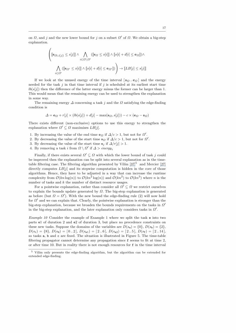
Example 10 Consider the example of Example 1 where we split the task e into two

parts e1 of duration 2 and e2 of duration 3, but place no precedence constraints on

these new tasks. Suppose the domains of the variables are D(sa) = 0, D(sb) = 2,D(sc) = 8, D(sd) = [ 0 .. 2 ], D(se1) = [ 2 .. 6 ], D(se2) = [ 2 .. 5 ], D(sf) = [ 2 .. 14 ],

so tasks a, b and c are fixed. The situation is illustrated in Figure 5. The time-table

filtering propagator cannot determine any propagation since f seems to fit at time 2,

or after time 10. But in reality there is not enough resources for f in the time interval

5 Vilım only presents the edge-finding algorithm, but the algorithm can be extended forextended edge-finding.

18

0 2 4 6 8 10 12 14

d

e1

f

16 18 20

ab

c

bc

a

e2

e1 e2

0 2 4 6 8 10 12 14

d

e1

f

16 18 20

ab

c

bc

a

e2

e1 e2

Fig. 5 (a) A example of propagation of the cumulative constraint using edge-finding. (b) theresult of propagating after the first step of stepwise edge-finding

[ 2 .. 10 ] since this must include the tasks b, c, e1, and e2. The total amount of resource

available here is 5 × 8 = 40, but 12 are taken by b and 8 are taken by c, e1 requires

4 resource units somewhere in this interval, and e2 required 6 resource units. Hence

there are only 10 resource units remaining in the interval [ 2 .. 10 ]. Starting f at time 2

requires at least 12 resource units be used within this interval hence this is impossible.

The edge-finding condition holds for Ω = b, c, e1, e2 and f. Now rest(c, 2) =

10 − (5 − 2) × (10 − 8) = 4 for Ω′ = c. The lower bound calculated is LB[f] =

8 + d4/2e = 10. The naıve explanation is J2 ≤ sfK ∧ J2 ≤ sbK ∧ Jsb ≤ 2K ∧ J2 ≤se1K ∧ Jse1 ≤ 6K ∧ J2 ≤ se2K ∧ Jse2 ≤ 5K ∧ J8 ≤ scK ∧ Jsc ≤ 8K→ J10 ≤ sfK.

The big-step explanation ensures that each task in Ω\Ω′ uses at least the amount of

resources in the interval [ 2 .. 10 ] as the reasoning above. It is J2 ≤ sfK∧J2 ≤ sbK∧Jsb ≤4K ∧ J2 ≤ se1K ∧ Jse1 ≤ 8K ∧ J2 ≤ se2K ∧ Jse2 ≤ 7K ∧ J8 ≤ scK ∧ Jsc ≤ 8K→ J10 ≤ sfK.

Now let us consider the pointwise explanation. If we restrict ourselves to use Ω for

calculating the new lower bound we determine LB[j] = 2+d(30−(5−2)×(10−2))/2e =

5 and the big-step explanation is J2 ≤ sfK ∧ J2 ≤ sbK ∧ Jsb ≤ 4K ∧ J2 ≤ se1K ∧ Jse1 ≤8K ∧ J2 ≤ se2K ∧ Jse2 ≤ 7K ∧ J2 ≤ scK ∧ Jsc ≤ 8K → J5 ≤ sfK, which results in the

situation shown in Figure 5(b). We then detect that edge-finding condition now holds

for Ω′ = c which creates a new lower bound 10, and explanation J5 ≤ sfK ∧ J8 ≤scK∧ Jsc ≤ 8K→ J10 ≤ sfK. The original big-step explanation is broken into two parts,

each logical stronger than the original.

For the original big-step explanation ∆ = 30 + 2× (2 + 6− 2)− 5× (10− 2) = 2.

We cannot use this to improve the explanation since it is not large enough. But for the

second explanation in the pointwise approach ∆ = 10+2×(5+6−8)−5×(10−8) = 6.

We could weaken the second explanation (corresponding the point 3 in the enumeration

on the page 17) to J3 ≤ sfK∧ J8 ≤ scK∧ Jsc ≤ 8K→ J10 ≤ sfK because ∆/r[f] = 6/2 =

3 > 1. 2

We have not yet implemented edge-finding with explanation, since the problems we

examine are not highly cumulative and for such problems edge-finding filtering cannot

compete with time-table filtering. It remains interesting future work to experimentally

compare different approaches to edge-finding filtering with explanation.

19

7 Resource-Constrained Project Scheduling Problems

Resource-constrained project scheduling problems (Rcpsp) appear as variants, exten-

sions and restrictions in many real-world scheduling problems. Therefore we test the

time, task decomposition and the explaining cumulative propagator on the well-known

Rcpsp benchmark library PSPLib [?].

An Rcpsp is denoted by a triple (T,A,R) where T is a set of tasks, A a set of

precedences between tasks and R is a set of resources. Each task i has a duration d[i]

and a resource usage r[k, i] for each resource k ∈ R. Each resource k has a resource

capacity c[k].

The goal is to find either a schedule or an optimal schedule with respect to an

objective function where a schedule s is an assignment which meets the following

conditions

∀i j ∈ A : s[i] + d[i] ≤ s[j]

∀t ∈ [ 0 .. tmax − 1 ] ,∀k ∈ R :∑

i∈T :s[i]≤t<s[i]+d[i]

r[k, i] ≤ c[k] ,

where tmax is the planning horizon. For our experiments we search for a schedule which

minimises the makespan tms such that s[i] + d[i] ≤ tms holds for i = 1, . . . , n .

The following code gives a basic Zinc model for the Rcpsp problem.

RCPSP basic model.zinc

% Parametersint: t_max; % planning horizonenum Tasks; % set of tasksenum Resources; % set of resourcesint: n = card(Tasks); % number of tasksarray[Tasks] of int: d; % durations of tasksarray[Tasks] of set of Tasks: suc; % successors of each taskarray[Resources, Tasks] of int: r; % resource usagearray[Resources] of int: c; % resource limit

% Variablesarray[Tasks] of var 0..t_max: s; % start times of tasksvar 0..t_max: makespan;

% Precedence constraintsconstraint

forall ( i in Tasks, j in suc[i] ) ( s[i] + d[i] <= s[j] );% Resource constraints

constraintforall ( k in Resources )( cumulative(array1d(1..n,s), array1d(1..n,d), [ r[k,i] | i in Tasks], c[k]));% Makespan constraints

constraintforall ( i in Tasks where suc[i] == )( s[i] + d[i] <= makespan );% (Redundant) Non-overlap constraints

constraintforall ( i, j in Tasks, k in Resources

where i < j /\ r[k,i] + r[k,j] > c[k] )( s[i] + d[i] <= s[j] \/ s[j] + d[j] <= s[i] );% Objective function

solve minimize makespan;

20

A Zinc data file representing the problem of Example 1 is

RCPSP run ex.dzn

t_max = 20;enum Tasks = ta, tb, tc, td, te, tf ;enum Resources = single ;d = array1d(Tasks, [2,6,4,2,5,6]);suc = array1d(Tasks, [tb,tc,,te,,]);r = array2d(Resources,Tasks,[1,2,4,2,2,2]);c = array1d(Resources,[5]);

In practice we share the Boolean variables generated inside the cumulative con-

straints as described in Section 5.1 (by common sub-expression elimination) and add

redundant constraints as described in Section 5.2 when using the TaskD decompo-

sition. We also add redundant non-overlap constraints for each pair of tasks whose

resource usages make them unable to overlap. Moreover, the planning horizon tmaxwas determined as the makespan of the first solution found by selection of the start

time variable with the smallest lower bound (if a tie occurs then the lexicographic

least variable) and assignment of the variable to its lower bound. The initial domain

of each variable s[i] was determined as Dinit(s[i]) = [ p[i] .. tmax − q[i] ] where p[i] is

the duration of the longest chain of predecessor tasks, and q[i] is the duration of the

longest chain of successor tasks.

In the remainder of this section we discuss alternative search strategies.

7.1 Search using Serial Scheduling Generation

The serial scheduling generation scheme (serial Sgs) is one of basic deterministic algo-

rithms to assign stepwise a start time to an unscheduled task. It incrementally extends

a partial schedule by choosing an eligible task—i.e. all of whose predecessors are fixed

in the partial schedule—and assigns it to its earliest start time with respect to the

precedence and resource constraints. For more details about SGS, different methods

based on it, and computational results in Operations Research see [15,21,22].

Baptiste and Le Pape [3] adapt serial Sgs for a constraint programming framework.

For our experiments we use a form where we do not apply their dominance rules, and

where we impose a lower bound on the start time instead of posting the delaying

constraint “task i executes after at least one task in S”.

1. Select an eligible unscheduled task i with the earliest start time t = lb(s[i]). If there

is a tie between some tasks then select that one with the minimal latest start time

ub(s[i]). If still tied then choose the lexicographic least task. Create a choice point.

2. Left branch: Extend the partial schedule by setting s[i] = t. If this branch fails then

go to the right branch; Otherwise go to step 1.

3. Right branch: Delay task i by setting s[i] ≥ t′ where t′ = minlb(s[j]) + d[j] | j ∈T : lb(s[j]) + d[j] > lb(s[i]), that is, the earliest end time of the concurrent tasks.

If this branch fails then backtrack to the previous choice point; Otherwise go to

step 1.

The right branch uses the dominance rule that amongst all optimal schedules there

exists one where every task starts either at the first possible time or immediately after

the end of another task. Therefore, the imposing of the new lower bound is sound,

21

no solution is lost for the considered problem. If we add side constraints then this

assumption could be invalid.

Note that we use this search strategy with branch and bound, where whenever a

new solution is found (with makespan = t), a constraint requiring a better solution

(makespan < t) is dynamically (globally) added during the search.

7.2 Search using Variable State Independent Decaying Sum

The SAT decision heuristic Variable State Independent Decaying Sum (Vsids) [28] is a

generic search approach that is currently almost universally used in DPLL SAT solvers.

Each variable is associated with a dynamic activity counter that is increased when the

variable is involved in a failure. Periodically, all counters are reduced, thus decaying.

The unfixed variable with the highest activity is selected to branch on at each stage.

Benchmark results by Moskewicz [28] shows that Vsids performs better on average on

hard problems than other heuristics.

To use Vsids in a lazy clause generation solver, we ask the SAT solver what its

preferred literal for branching on is. This corresponds to an atomic constraint x ≤ d

or x = d and we branch on x ≤ d ∨ x > d or x = d ∨ x 6= d. Note that the search

is still controlled by the FD search engine, so that we use its standard approach to

implementing branch-and-bound to implement the optimisation search.

Normally SAT solvers use dichotomic restart search for optimisation as the SAT

solver itself does not have optimisation search built in. That is assuming minspan is

the current lower bound on makespan, and a new solution is found with makespan = t

we let t′ = b(t+ minspan)/2c and solve the satisfaction problem to find a makespan in

the range[

minspan .. t′]. If we find a solution at t′′ we continue the process, otherwise

we reset minspan to t′ + 1 and solve the satisfaction problem to find a makespan in

the range [ minspan .. t− 1 ]. Note that when a satisfaction search fails the nogoods

generated in that search are not valid for subsequent searches (since they make use of

the assumption makespan ≤ t′.The combination of Vsids and branch and bound is much stronger since in the

continuation of the search with a better bound, the activity counts at the time of

finding a new better solution are used in the same part of the search tree, and all

nogoods generated remain valid.

Restarting is shown to be beneficial in SAT solving (and CSP solving) in speeding

up solution finding, and being more robust on hard problems. On restart the set of

nogoods has changed as well as the activity of variables, so the search will take a very

different path. We also use Vsids search with restarting, which we denote Restart. 6

7.3 Hybrid Search Strategies

One drawback of Vsids is that at the beginning of the search the activity counters are

only related to the clauses occurring in the original model, and not to any conflict. This

is exacerbated in lazy clause generation where many of the constraints of the problem

may not appear at all in the clause database initially. This can lead to poor decisions

6 Note that restarting with Sgs is not very attractive since we rarely learn anything thatchanges the Sgs search decisions, we effectively just continue the same search.

22

in the early stages of the search. Our experiments support this, there are a number of

“easy” instances which Sgs can solve within a small number of choice points, where

Vsids requires substantially more.

In order to avoid these poor decisions we consider a hybrid search strategy. We

use Sgs for the first 500 choice points and then restart the search with Vsids. The

Sgs search may solve the whole problem if it is easy enough, but otherwise it sets the

activity counters to meaningful values so that Vsids starts concentrating on meaningful

decisions. We denote this search as Hot Start, and the version where the secondary

Vsids search also restarts as Hot Restart.

8 Experiments

We carried out extensive experiments on Rcpsp instances comparing our approaches to

decomposition without explanation, global cumulative propagators from sicstus and

eclipse, as well as a state-of-the-art exact solving algorithm [23]. Detailed results are

available at http://www.cs.mu.oz.au/~pjs/rcpsp.

We use two suites of benchmarks. The library PSPLib [1,?] contains the four classes

J30, J60, J90, and J120 consisting of 480 instances of 30, 60, 90, and 120 tasks respec-

tively. We also use a suite (BL) of 40 highly cumulative instances with either 20 or 25

tasks constructed by Baptiste and Le Pape [3].

The experiments were run on a X86-64 architecture running GNU/Linux and a

Intel(R) Xeon(R) CPU E54052 processor with 2GHz. The code was written in Mer-

cury using the G12 Constraint Programming Platform and compiled with the Mercury

Compiler and grade hlc.gc.trseg. Each run was given a 10 minute limit.

We compare 4 different implementations of cumulative with explanation: (t) the

TimeD decomposition of Section 5.1, (s) the TaskD decomposition of Section 5.2, (e)

a task decomposition using end times (e), and (g) a global cumulative using time-

table filtering with explanation. The global cumulative uses pointwise explanations

for consistency and iterative pointwise explanations for filtering. We experimented

with other forms of explanations for the global cumulative but they were inferior

for hard instances, although surprisingly not that bad (about 15% worse in average

except for naıve explanations which behave terribly). The present implementation of

the global cumulative recalculates the resource profile on each invocation which could

be significantly improved by making it incremental. Profiling on a few instances showed

that more than the half of the time was spent in propagation of cumulative.

8.1 Results on J30 and BL instances

The first experiment compares different decompositions and search on the smallest

instances J30 and BL. We compare Sgs, Vsids, Restart and the hybrid search ap-

proaches using our 4 different propagation with explanation approaches. The results

are shown in Table 1 and 2. For J30 we show the number of problems solved (#svd),

(cmpr(477)) the average solving time in seconds and number of failures on the 477

problems that all approaches solved, and (all(480)) average solving time in seconds

and number of failures on all 480 problems within the execution.7 Note that we shall

7 This means that for problems that time out the number of failures is substantially largerthan those which were solved before timeout.

23

Table 1 Results on J30 instances

search model #svd cmpr(477) all(480)time fails time fails

Sgs

s 477 2.13 3069 5.86 5375e 477 2.19 3054 5.93 5331t 480 0.87 2339 2.83 4230g 480 0.73 1977 3.04 3919

Vsids

s 480 1.20 2128 1.63 2984e 480 0.46 1504 0.77 2220t 480 0.26 1002 0.33 1271g 480 0.15 797 0.20 1058

Restart

s 480 0.50 1483 0.93 2317e 480 0.43 1368 0.80 2128t 480 0.24 856 0.33 1174g 480 0.15 777 0.22 1093

Hot Startt 480 0.21 779 0.34 1220g 480 0.12 706 0.17 956

Hot Restartt 480 0.26 884 0.35 1231g 480 0.13 727 0.21 1058

Table 2 Results on BL instances

search model #svd all(40) #svd fails(4000)

Sgs

s 40 2.51 9628 24 0.18 1261e 40 2.63 9443 24 0.15 1144t 40 0.82 5892 29 0.04 781g 40 0.88 5723 30 0.05 860

Vsids

s 40 0.79 4436 31 0.16 1115e 40 0.77 4104 30 0.15 1025t 40 0.22 2540 34 0.04 661g 40 0.20 2039 37 0.04 605

Restart

s 40 0.88 4549 31 0.17 1169e 40 1.46 5797 32 0.17 1135t 40 0.13 1626 35 0.05 603g 40 0.14 1568 36 0.04 546

Hot Startt 40 0.10 1448 36 0.04 680g 40 0.12 1485 36 0.04 593

Hot Restartt 40 0.15 1829 35 0.05 719g 40 0.25 2460 36 0.05 680

use similar comparisons and notation in future tables. For the BL problems the results

are shown in Table 2. We show the number of solved problems, (all(40)) average solving

time and number of failures with a 10 minute limit (on all 40 instances), as well as

fails(4000) with a 4000 failure limit.

Of the decompositions the TimeD decomposition is clearly the best being almost

twice as fast as the TaskD decompositions. This is presumably the effect of the stronger

propagation. Note that these are the smallest problems where its relative disadvantage

in size is least visible. The global is usually significantly better than the TimeD de-

composition: it usually requires less search and can be up to twice as fast. Interestingly

sometimes the TimeD decomposition is faster which may reflect the fact that it is (au-

tomatically) a completely incremental implementation of the cumulative constraint.

For these small problems the best search strategy is Hot Start since the overhead of

restarting Vsids does not pay off for these simple problems.

24

Table 3 Results of the FD solvers on the J30 instances

solver #svd cmpr(364) all(480)

sicst

us default 418 0.22 337 87.43 141791

global 415 0.40 331 94.01 76533eclipse cumu 368 13.98 26469 154.79 365364

ef 366 18.33 21717 157.43 173445ef3 368 16.61 17530 155.87 155142

G12 FD +t 404 1.79 5701 104.38 641185

Sgs +t 480 0.01 75 2.83 4230Sgs +g 480 0.01 70 3.04 3919

Table 4 Results of the FD solvers on the BL instances

solver #svd cmpr(7) all(40)

sicst

us default 32 2.87 25241 195.05 1896062

global 39 0.90 3755 18.36 63310

eclipse cumu 7 178.90 352318 526.61 2231026

ef 37 43.06 53545 102.60 229332ef3 37 35.56 39836 81.47 144051

G12 FD +t 30 6.71 72427 216.87 2650886

Sgs + t 40 0.01 268 0.82 5892Sgs + g 40 0.01 278 0.88 5723

The results on the BL instances show that approaches using TimeD or the global

propagator and Vsids could solve between 6 and 9 instances more than the base ap-

proach (FE) of Baptiste and Le Pape [3] within 4000 failures. Their “left-shift/right-

shift” approach could solve all 40 instances in 30 minutes, with an average of 3634

failures and 39.4 seconds on a 200 MHz machine. All our approaches with TimeD and

Vsids find the optimal solution faster and in fewer failures (between a factor of 1.39

and 2.4).

Next we compare the TimeD decomposition (Sgs+t) and global propagator (Sgs+g)

against implementations of cumulative in sicstus v4.0 (default, and with the flag

global) and eclipse v6.0 (using its 3 cumulative versions from the libraries cumulative,

edge finder and edge finder3). We also compare against (FD+t) a decomposition

without explanation (a normal FD solver) executed in the G12 system. All approaches

use the Sgs search strategy.

The results are shown in the Tables 3 and 4. Clearly the more expensive edge-finding

filtering algorithms are not advantageous on the J30 examples, but they do become

significantly beneficial on the highly cumulative BL instances. We can see that none

of the other approaches compare to the lazy clause generation approaches. The best

solver without learning is the sicstus cumulative with global flag. Clearly nogoods

are very important to fathom search space.

While the TimeD decomposition clearly outperforms TaskD on these small exam-

ples, as the planning horizon grows at some point TaskD should be better, since its

model size is independent of the planning horizon. We took the J30 examples and

multiplied the durations and planning horizon by 10 and 100. We compare the TimeD

decomposition versus the (e) end-time TaskD decomposition (which is slightly better

than start-time (s)) and the global cumulative (g). The results are shown in Table 5.

First we should note that simply increasing the durations makes the problems sig-

25

Table 5 Results on the modified J30 instances

search duration model #svd cmpr(462) all(480)

Sgs

1×e 477 0.11 542 5.93 5331t 480 0.08 501 2.83 4230g 480 0.05 371 3.04 3919

10×e 471 0.58 1812 14.76 9512t 476 1.03 676 11.04 4972g 478 0.10 393 4.92 4291

100×e 466 4.87 4586 23.40 10813t 465 15.58 724 35.02 1582g 477 0.70 403 8.51 3684

Vsids

1×e 480 0.06 318 0.77 2220t 480 0.04 249 0.33 1271g 480 0.02 151 0.20 1058

10×e 480 0.18 821 4.23 4213t 480 0.63 1210 4.84 2714g 480 0.06 284 0.39 1215

100×e 474 1.32 2031 12.36 4224t 469 9.88 9229 27.35 9707g 480 0.62 1296 3.15 2360

nificantly more difficult. While the TimeD decomposition is still just better than the

TaskD decomposition for the 10× extended examples, it is inferior for scheduling prob-

lems with very long durations. The most important result visible from this experiment

is the advantage of the global propagator over the TimeD decomposition as the plan-

ning horizon gets larger. The global propagator is by far the best approach for the

larger problems since it has the O(n2) complexity of the TaskD decomposition but the

same propagation strength as the much stronger TimeD decomposition. Note also how

the failures get dramatically worse for the TimeD decomposition using Vsids as the

problem grows. This illustrates how the large number of Booleans in the decomposition

makes the Vsids heuristic less effective.

8.2 Results on J60, J90 and J120

We now examine the larger instances J60, J90 and J120 from PSPLib. For J60 we

compare the most competitive search approaches from the previous subsection: Vsids,

Restart, Hot Start and Hot Restart using the TimeD decomposition and global

propagator. For this suite our solvers cannot solve all 480 instances within 10 minutes.

The results are presented in Table 6. For these examples we show the average distance

of the makespan from our best solution to the best known solution from PSPLib (most

of which are generated by specialised heuristic methods), as well as the usual time and

number of failures comparisons. Many of these are currently open problems. Our best

approaches close 24 open instances. While all of the methods are quite competitive we

see that restarting is valuable for improving the average distance from the best known

optimal, and the hybrid approach Hot Restart is marginally more robust than the

others. Interestingly Hot Start can clearly force the search into a less promising area

than just plain Vsids.

For the largest instances J90 and J120 we ran only Hot Restart since it is the most

robust search strategy, using the TimeD decomposition and the global propagator. The

results are presented in the Table 7 which shows that the global propagator is superior

26

Table 6 Results on J60 instances for TimeD and global propagator

search model #svd avg. dist. cmpr(425) all(480)

Vsidst 426 4.4 4.85 7216 72.71 41891g 430 6.2 2.99 4943 67.13 52016

Restartt 428 4.5 3.53 5139 68.04 61558g 430 3.7 2.50 4418 66.01 60518

Hot Startt 429 9.3 2.91 4629 66.64 52812g 428 18.1 2.93 4848 66.19 57823

Hot Restartt 429 4.0 3.28 4982 66.60 60146g 430 3.9 2.60 4658 66.18 60652

Table 7 Results on J90 and J120 instances for TimeD and global propagator

J90search model #svd avg. dist. cmpr(395) all(480)

Hot Restartt 396 7.5 4.16 4364 108.90 90582g 397 7.5 3.34 3950 108.57 90134

J120search model #svd avg. dist. cmpr(274) all(600)

Hot Restartt 274 9.7 8.50 8543 329.46 234897g 282 9.6 5.40 7103 324.51 242343

Table 8 Comparison between Laborie’s method, Hot Restart + t and g

J60 J90 J1201.4 GHz 15s 300s 1800s 15s 300s 1800s 15s 300s 1800sLaborie - 84.2 85.0 - 78.5 79.4 - 41.3 41.7

Hot Restart + t 84.8 89.2 89.4 79.8 81.7 82.5 42.3 45.2 45.7Hot Restart + g 85.8 89.0 89.6 80.0 81.9 82.7 42.7 45.8 47.0

2.0 GHz 10s 200s 600s∗ 10s 200s 600s∗ 10s 200s 600s∗

to the TimeD decomposition. In total we close 15 and 27 open instances in J90 and

J120 respectively (see Appendix A for more details).

We compare our best methods Hot Restart with either t or g to the method by

Laborie [23] that uses minimal critical sets as a branching scheme and was implemented

in ILOG Scheduler 6.1 using as filtering algorithms among others time-table and

edge-finding. His method is the best published method so far on the J60, J90, and

J120 instances.

Table 8 shows the percentage of solved instances within a maximal solve time. We

give an equivalent time to our solver taking into account the speeds of the processors:

2.0GHz vs. 1.4GHz. At the top of the table is the time cutoff for a 1.4GHz processor,

and at the bottom the approximately equivalent cutoff times for a 2.0GHz machine.

Note, that all ∗ marked 2.0GHz times are much lower than the equivalent time for the

1.4GHz processor. Clearly this comparison can only be seen as indicative.

Our methods clearly outperforms Laborie’s method: for every class our methods

were able to solve more problems within 10s than they could solve in half an hour

respectively on their machine. Interestingly, our solver could not solve six instances

which were solved by others. We can also see the advantage of the global propagator

increases with increasing problem size.

Finally we used Hot Start + g to try to improve lower bounds of the remaining

open problems, by searching for a solution to the problem with the makespan varying

27

from the best known lower bound to the best known upper bound from PSPLib. In

this way we closed 6 more problems and improved 78 lower bounds (see Appendix B).

9 Conclusion

We present a new approach solving Rcpsp problems by using cumulative constraints

with explanation in a lazy clause generation system. First we show that modelling

cumulative constraints by decomposition and using lazy clause generation is highly

competitive. We then improve this by building a global cumulative propagator with ex-

planation. Benchmarks from the PSPLib show the strong power of nogoods and Vsids

style search to fathom a large part of the search space. Without building complex spe-

cific global propagators or highly specialised search algorithms we are able to compete

with highly specialised Rcpsp solving approaches and close 71 open problems.

Acknowledgements We would like to thank Phillipe Baptiste for suggesting this line ofenquiry. NICTA is funded by the Australian Government as represented by the Department ofBroadband, Communications and the Digital Economy and the Australian Research Council.

References

1. PSPLib — project scheduling problem library. Http://129.187.106.231/psplib/. 23.04.20092. Aggoun, A., Beldiceanu, N.: Extending CHIP in order to solve complex scheduling and

placement problems. Mathematical and Computer Modelling 17(7), 57–73 (1993)3. Baptiste, P., Le Pape, C.: Constraint propagation and decomposition techniques for highly

disjunctive and highly cumulative project scheduling problems. Constraints 5(1-2), 119–139 (2000)

4. Blazewicz, J., Lenstraand, J.K., Rinnooy Kan, A.H.G.: Scheduling subject to resourceconstraints: classification and complexity. Discrete Applied Mathematics 5, 11–24 (1983)

5. Carlier, J., Pinson, E.: Jackson’s pseudo-preemptive schedule and cumulative schedul-ing problems. Discrete Applied Mathematics 145(1), 80–94 (2004). DOI10.1016/j.dam.2003.09.009

6. Caseau, Y., Laburthe, F.: Cumulative scheduling with task intervals. In: Procs. of the1996 Joint International Conference and Symposium on Logic Programming, pp. 363–377.MIT Press (1996). URL citeseer.ist.psu.edu/caseau94cumulative.html

7. Claessen, K., Een, N., Sheeran, M., Sorensson, N., Voronov, A., Akesson, K.: Sat-solvingin practice, with a tutorial example from supervisory control. Discrete Event DynamicSystems 19(4), 495–524 (2009). DOI 10.1007/s10626-009-0081-8

8. Davis, M., Logemman, G., Loveland, D.: A machine program for theorem proving. Com-munications of the ACM 5(7), 394–397 (1962)

9. Dechter, R., Meiri, I., Pearl, J.: Temporal constraint networks. Artificial Intelligence 49,61–95 (1991)

10. Demeulemeester, E.L., Herroelen, W.S.: New benchmark results for the resource-constrained project scheduling problem. Management Science 43(11), 1485–1492 (1997)

11. Een, N., Sorensson, N.: An extensible SAT-solver. In: E. Giunchiglia, A. Tacchella (eds.)Proceedings of SAT 2003, LNCS, vol. 2919, pp. 502–518 (2003)

12. El-Kholy, A.O.: Resource feasibility in planning. Ph.D. thesis, Imperial College, Universityof London (1996)

13. Erschler, J., Lopez, P.: Energy-based approach for task scheduling under time and resourcesconstraints. In: 2nd International Workshop on Project Management and Scheduling,, pp.115–121 (1990)

14. Feydy, T., Stuckey, P.J.: Lazy clause generation reengineered. In: I. Gent (ed.) Proceedingsof the 15th International Conference on Principles and Practice of Constraint Program-ming, LNCS, vol. 5732, pp. 352–366. Springer-Verlag (2009). DOI 10.1007/978-3-642-04244-7 29

28

15. Hartmann, S., Kolisch, R.: Experimental evaluation of state-of-the-art heuristics for theresource-constrained project scheduling problem. EJOR 127(2), 394–407 (2000). DOI10.1016/S0377-2217(99)00485-3

16. Jussien, N.: The versatility of using explanations within constraint programming. Re-search Report 03-04-INFO, Ecole des Mines de Nantes, Nantes, France (2003). URLhttp://www.emn.fr/jussien/publications/jussien-RR0304.pdf

17. Jussien, N., Barichard, V.: The PaLM system: explanation-based constraint program-ming. In: Proceedings of Techniques foR Implementing Constraint programming Systems(TRICS 2000), pp. 118–133 (2000). URL http://www.emn.fr/jussien/publications/jussien-WCP00.pdf

18. Jussien, N., Debruyne, R., Boizumault, P.: Maintaining arc-consistency within dynamicbacktracking. In: Principles and Practice of Constraint Programming – CP 2000, no. 1894in Lecture Notes in Computer Science, pp. 249–261. Springer-Verlag, Singapore (2000)

19. Jussien, N., Lhomme, O.: Local search with constraint propagation and conflict-basedheuristics. Artificial Intelligence 139(1), 21–45 (2002)

20. Katsirelos, G., Bacchus, F.: Generalized nogoods in csps. In: M.M. Veloso, S. Kambham-pati (eds.) National Conference on Artificial Intelligence, pp. 390–396. AAAI Press / TheMIT Press (2005)

21. Kolisch, R.: Serial and parallel resource-constrained project scheduling methods revisited:Theory and computation. EJOR 90(2), 320–333 (1996). DOI 10.1016/0377-2217(95)00357-6

22. Kolisch, R., Hartmann, S.: Experimental investigation of heuristics for resource-constrained project scheduling: An update. EJOR 174(1), 23–37 (2006). DOI10.1016/j.ejor.2005.01.065

23. Laborie, P.: Complete MCS-based search: Application to resource constrained projectscheduling. In: L.P. Kaelbling, A. Saffiotti (eds.) Proceedings IJCAI 2005, pp. 181–186.Professional Book Center (2005). URL http://ijcai.org/papers/0571.pdf

24. Lahrichi, A.: Scheduling: the notions of hump, compulsory parts and their use in cumula-tive problems. C. R. Acad. Sci., Paris, Ser. I, Math. 294(2), 209–211 (1982)

25. Liess, O., Michelon, P.: A constraint programming approach for the resource-constrainedproject scheduling problem. Annals of Operations Research 157(1), 25–36 (2008). DOI10.1007/s10479-007-0188-y

26. Marriott, K., Nethercote, N., Rafeh, R., Stuckey, P.J., Garcia de la Banda, M., Wallace,M.G.: The design of the Zinc modelling language. Constraints 13(3), 229–267 (2008).DOI 10.1007/s10601-008-9041-4

27. Mercier, L., Van Hentenryck, P.: Edge finding for cumulative scheduling. INFORMS Jour-nal on Computing 20(1), 143–153 (2008). DOI 10.1287/ijoc.1070.0226

28. Moskewicz, M.W., Madigan, C.F., Zhao, Y., Zhang, L., Malik, S.: Chaff: Engineering anefficient SAT solver. In: Design Automation Conference, pp. 530–535. ACM, New York,NY, USA (2001). DOI 10.1145/378239.379017

29. Nuijten, W.P.M.: Time and resource constrained scheduling. Ph.D. thesis, EindhovenUniversity of Technology (1994)

30. Ohrimenko, O., Stuckey, P., Codish, M.: Propagation via lazy clause generation. Con-straints 14(3), 357–391 (2009)

31. Ohrimenko, O., Stuckey, P.J., Codish, M.: Propagation = lazy clause generation. In: Procs.of the CP2007, LNCS, vol. 4741, pp. 544–558. Springer (2007). DOI 10.1007/978-3-540-74970-7 39

32. Schulte, C., Stuckey, P.: Efficient constraint propagation engines. ACM Transactions onProgramming Languages and Systems 31(1), Article No. 2 (2008)

33. Schutt, A.: Entwicklung suchraumeinschrankender Verfahren zur Constraint-basiertenLosung kumulativer Ressourcenplanungsprobleme. Master’s thesis, Humboldt-Universitatzu Berlin (2006)

34. Schutt, A., Feydy, T., Stuckey, P.J., Wallace, M.G.: Why cumulative decomposition is notas bad as it sounds. In: I. Gent (ed.) Proceedings of the 15th International Conferenceon Principles and Practice of Constraint Programming, LNCS, vol. 5732, pp. 746–761.Springer-Verlag (2009)

35. Schutt, A., Wolf, A., Schrader, G.: Not-first and not-last detection for cumulative schedul-ing in O(n3 logn). In: Declarative Programming for Knowledge Management, Lec-ture Notes in Computer Science, vol. 4369, pp. 66–80. Springer-Verlag (2006). DOI10.1007/11963578. INAP 2005 — 16th International Conference on Applications of Declar-ative Programming and Knowledge Management

29

36. Vilım, P.: Computing explanations for the unary resource constraint. In: Integration of AIand OR Techniques in Constraint Programming for Combinatorial Optimization Problems,LNCS, vol. 3524, pp. 396–409. Springer-Verlag (2005). DOI 10.1007/11493853 29. URLhttp://kti.ms.mff.cuni.cz/ vilim/cpaior2005.pdf

37. Vilım, P.: Edge finding filtering algorithm for discrete cumulative resources in O(kn logn).In: Principles and Practice of Constraint Programming - CP 2009, LNCS, vol. 5732, pp.802–816. Springer-Verlag (2009). DOI 10.1007/978-3-642-04244-7 62

30

Table 9 Closed instancesJ60

Instance 5 10 9 2 9 4 14 1 14 10 17 8 21 9 25 1Makespan 81 82 87 61 72 85 89 114

Instance 25 3 25 56 25 9 30 5 30 7 30 10 41 1 41 2Makespan 113 98 99 76 86 86 122 113

Instance 41 6 41 9 46 4 46 5 46 6 46 7 46 9 46 10Makespan 134 131 74 91 90 78 69 88

J90

Instance 5 1 5 2 21 28 21 4 21 5 21 6 21 9 21 10Makespan 78 93 116 106 112 106 121 109

Instance 26 57 37 1 37 4 37 5 37 88 37 9 37 108 42 2Makespan 85 110 123 126 119 123 123 102

Instance 42 7 42 10Makespan 87 90

J120

Instance 1 3 1 8 1 10 2 2 8 39 21 2 21 7 22 3Makespan 125 109 108 75 95 117 111 96

Instance 22 8 28 4 28 8 28 9 28 10 29 4 41 2 41 9Makespan 103 112 99 98 116 80 141 121

Instance 42 5 42 8 48 1 48 5 48 8 48 9 48 10 49 3Makespan 120 113 100 110 116 113 111 96

Instance 49 4 49 5 49 7 49 10 50 48

Makespan 96 89 99 97 100

A Closed instances

In the Table 9 we list all previously open instances (wrt. [1], [23], and [25]) with their optimalmakespan which were closed by Hot Restart with the global cumulative or some othermethod. In the last case a footnote is given for these instances. The optimal makespan ofalmost all closed instances correspond to the previously best known upper bound found bylocal search heuristics, except for the J120 instances 8 3 and 48 5 where our solver could reducethem by 1 to 95 and 110 resp. Note that Hot Restart with the TimeD decomposition wasalso capable of closing 63 of these instances.

In total 71 instances of 504 open instances are closed with 64 instances by Hot Restartwith cumulative (g), one by Hot Restart with TimeD, one by Vsids with cumulative, fourby the lower bound computation (see Appendix B) and one by a combination of two methods.9

B New lower bounds

We tried to compute new lower bounds using Hot Start with global cumulative for theremaining open instances. These experiments were carried out on the same machine with thesame (overall) time limit. (cf. Sec. 8). We set the makespan to the best known lower bound,and tried to find a solution, if this failed we increased the makespan by one and re-solved. Ifa solution was found this is the optimal, if we can prove failure for a given makespan we haveincreased the lower bound. If the increased lower bound equaled the best known upper boundwe have proved the optimality of the upper bound and closed the instance as well.

6 Closed by Vsids + g.7 Closed by Hot Restart + t.8 Closed by lower bound computation by proof of the equality of lower and best known

upper bound.9 Closed by Hot Restart and lower bound computation. Hot Restart decreased the pre-

viously best known upper bound to 95 and the lower bound computation proved the optimalityof this new bound.

31

Table 10 New lower bounds on all instancesJ60

Instance 9 3 9 5 9 6 9 8 9 9 9 10 25 2 25 4LB 99 80 105 94 98 88 95 105

Instance 25 6 25 7 25 8 25 10 29 2 29 9 30 2 41 3LB 105 88 95 107 123 105 69 89

Instance 41 5 41 10 45 3 45 4LB 109 105 133 101

J90

Instance 5 4 5 6 5 8 5 9 21 1 21 7 21 8 37 2LB 101 85 96 113 109 105 107 113

Instance 37 6 41 3 41 7 46 4LB 129 147 144 92

J120

Instance 1 1 6 8 7 2 7 3 7 6 8 2 8 4 8 6LB 104 140 113 97 115 101 91 84

Instance 9 4 26 2 26 4 26 5 26 7 26 8 26 9 26 10LB 84 158 160 138 144 167 160 177

Instance 27 2 27 5 27 7 27 10 28 7 29 3 34 8 42 1LB 109 105 118 110 108 96 86 106

Instance 46 1 46 2 46 3 46 5 46 7 46 9 46 10 47 1LB 171 186 162 135 155 156 174 129

Instance 47 2 47 4 47 5 47 9 48 3 48 6 48 7 49 2LB 126 119 125 140 109 102 105 108

Instance 53 3 53 4 53 9 54 7 54 10 60 2LB 105 137 155 108 107 82

In total this method closed 6 more instances (see Appendix A) and improved the lowerbound by 78 instances of the remaining 433 open instances. The improved lower bounds arelisted in Table 10.