
Geometric and Dual Approaches to Cumulative Scheduling
150
NNT : 2017SACLX119 T HÈSE DE DOCTORAT DE L’U NIVERSITÉ P ARIS -S ACLAY PRÉPARÉE À L’É COLE P OLYTECHNIQUE E COLE DOCTORALE N°580 Sciences et Technologies de l’Information et de la Communication Mathématiques et Informatique Par M. Nicolas Bonifas Geometric and Dual Approaches to Cumulative Scheduling Thèse présentée et soutenue à Paris, le 19 décembre 2017. Composition du Jury : M. Jean-Charles Billaut, Professeur, Université de Tours. Président M. Jacques Carlier, Professeur Émérite, UT Compiègne. Rapporteur M. Christian Artigues, Directeur de Recherche, LAAS-CNRS. Rapporteur Mme Catuscia Palamidessi, Directrice de Recherche, LIX-CNRS. Examinatrice M. Peter Stuckey, Professeur, Université de Melbourne. Examinateur M. Philippe Baptiste, Directeur de Recherche, LIX-CNRS. Directeur de thèse M. Jérôme Rogerie, Ingénieur R&D, IBM France. Co-directeur de thèse
-
Upload
khangminh22 -
Category
Documents
-
view
2 -
download
0
Transcript of Geometric and Dual Approaches to Cumulative Scheduling

NNT : 2017SACLX119
THÈSE DE DOCTORATDE
L’UNIVERSITÉ PARIS-SACLAYPRÉPARÉE À
L’ÉCOLE POLYTECHNIQUE
ECOLE DOCTORALE N°580Sciences et Technologies de l’Information et de la
Communication
Mathématiques et Informatique
Par
M. Nicolas Bonifas
Geometric and Dual Approaches toCumulative Scheduling
Thèse présentée et soutenue à Paris, le 19 décembre 2017.
Composition du Jury :M. Jean-Charles Billaut, Professeur, Université de Tours. PrésidentM. Jacques Carlier, Professeur Émérite, UT Compiègne. RapporteurM. Christian Artigues, Directeur de Recherche, LAAS-CNRS. RapporteurMme Catuscia Palamidessi, Directrice de Recherche, LIX-CNRS. ExaminatriceM. Peter Stuckey, Professeur, Université de Melbourne. ExaminateurM. Philippe Baptiste, Directeur de Recherche, LIX-CNRS. Directeur de thèseM. Jérôme Rogerie, Ingénieur R&D, IBM France. Co-directeur de thèse


Abstract
ContextThis work falls in the scope of mathematical optimization, and more pre-
cisely in constraint-based scheduling. This involves determining the start andend dates for the execution of tasks (these dates constitute the decision variablesof the optimization problem), while satisfying time and resource constraintsand optimizing an objective function.
In constraint programming, a problem of this nature is solved by a tree-based exploration of the domains of decision variables with a branch & boundsearch. In addition, at each node a propagation phase is carried out: necessaryconditions for the different constraints to be satisfied are verified, and values ofthe domains of the decision variables which do not satisfy these conditions areeliminated.
In this framework, the most frequently encountered resource constraint isthe cumulative. Indeed, it enables modeling parallel processes, which consumeduring their execution a shared resource available in finite quantity (such asmachines or a budget). Propagating this constraint efficiently is therefore ofcrucial importance for the practical efficiency of a constraint-based schedulingengine.
In this thesis, we study the cumulative constraint with the help of toolsrarely used in constraint programming (polyhedral analysis, linear program-ming duality, projective geometry duality). Using these tools, we propose twocontributions for the domain: the Cumulative Strengthening, and the O(n2 log n)Energy Reasoning.
Contributions
Cumulative Strengthening
We propose a reformulation of the cumulative constraint, that is to say thegeneration of tighter redundant constraints which allows for a stronger propa-
3

4
gation, of course without losing feasible solutions.This technique is commonly used in integer linear programming (cutting
planes generation), but this is one of its very first examples of a redundantglobal constraint in constraint programming.
Calculating this reformulation is based on a linear program whose size de-pends only on the capacity of the resource but not on the number of tasks, whichmakes it possible to precompute the reformulations.
We also provide guarantees on the quality of the reformulations thus ob-tained, showing in particular that all bounds calculated using these reformu-lations are at least as strong as those that would be obtained by a preemptiverelaxation of the scheduling problem.
This technique makes it possible to strengthen all propagations of the cumu-lative constraint based on the calculation of an energy bound, in particular theEdge-Finding and the Energy Reasoning.
This work was presented at the ROADEF 2014 conference [BB14] and waspublished in 2017 in the Discrete Applied Mathematics journal [BB17a].
O(n2 log n) Energy Reasoning
This work consists of an improvement of the algorithmic complexity of oneof the most powerful propagations for the cumulative constraint, namely theEnergy Reasoning, introduced in 1990 by Erschler and Lopez.
In spite of the very strong deductions found by this propagation, it is rarelyused in practice because of its cubic complexity. Many approaches have beendeveloped in recent years to attempt to make it usable in practice (machinelearning to use it wisely, reducing the constant factor of its algorithmic com-plexity, etc).
We propose an algorithm that computes this propagation with a O(n2 log n)complexity, which constitutes a significant improvement of this algorithm knownfor more than 25 years. This new approach relies on new properties of the cu-mulative constraint and on a geometric study.
This work was published in preliminary form at the CP 2014 conference[Bon14] and was published [Bon16] at the ROADEF 2016 conference, where itwas awarded 2th prize of the Young Researcher Award.

Remerciements
It may be that when we no longer know what to do,we have come to our real workand when we no longer know which way to go,we have begun our real journey.
The mind that is not baffled is not employed.The impeded stream is the one that sings.
(Wendell Berry)
Il est d’usage d’écrire quelques remerciements en introduction d’un manuscritde thèse, mais j’ai été tellement porté pendant mes études et mes années de doc-torat que cela me semble être la chose la plus naturelle du monde.
Avant tout, mes remerciements vont à ma famille, et à mes parents extraor-dinaires. Je mesure la chance que j’ai eu de grandir dans un environnementsécurisant, épanouissant, et aimant !
En ce qui concerne cette thèse, mes remerciements vont à mon directeur dethèse, Philippe Baptiste, qui a su m’indiquer des questions scientifiques dignesd’intérêt et a pris beaucoup de temps dans son emploi du temps chargé pourme guider. Du côté d’IBM, mes encadrants ont été Jérôme Rogerie, que je remer-cie pour ses conseils, son soutien, et de nombreuses discussions inattendues etéclairantes, ainsi que Philippe Laborie, qui m’a tant appris en optimisation, etqui a su trouver une réponse me permettant d’avancer à chaque question queje lui ai posée. C’était un bonheur de travailler avec vous. Merci aussi à PaulShaw et Éric Mazeran pour voir rendu cette thèse possible, ainsi qu’à tous mescollègues d’IBM, de l’équipe CP Optimizer et au-delà.
Merci à Jacques Carlier et Christian Artigues d’avoir accepté de relire cemanuscrit, ainsi qu’à Jean-Charles Billaut, Catuscia Palamidessi et Peter Stuckeyd’avoir bien voulu faire partie de mon jury.
Je voudrais aussi remercier toutes les personnes qui, tout autour du monde,m’ont invité à collaborer au cours de cette thèse, et notamment Christian Ar-tigues, Pierre Lopez (que je remercie tout particulièrement pour m’avoir in-
5
6
vité à travailler sur le raisonnement énergétique), Friedrich Eisenbrand, DanielDadush, Mark Wallace, Andreas Schutt, Yakov Zinder, Leo Liberti, Berthe Choueiryet François Clautiaux.
J’ai eu la chance de rencontrer au cours de ma formation des professeursextraordinaires. Au nombre de ceux qui m’ont marqués, je voudrais citer, parordre chronologique, Emmanuelle Grand et Françoise Routon, Gérard Vachet,Annick Pasini, Mariange Ramozzi-Doreau, Ronan Ludot-Vlasak, Jean-PierreLièvre, Stéphane Gonnord, Jacques Renault, Florent de Dinechin et FriedrichEisenbrand. Un mot tout particulier pour Mathias Hiron, qui forme d’unemanière remarquable des lycéens à l’algorithmique et à la programmation ausein de l’association France IOI. C’est d’eux que je m’efforce de m’inspirer lorsqueje me trouve parfois de l’autre côté du bureau.
Ces remerciements deviendraient une thèse à eux seuls si je devais saluertous ceux qui comptent pour moi, aussi je ne vais mentionner que les amis quiont eu un impact direct sur ce travail de thèse. Lucien, avec qui j’ai partagétrès jeune la découverte des mathématiques et de l’informatique. Mes amis deLausanne, avec qui j’ai passé de si bons moments et eu tant de discussions pas-sionnantes. Le club de plongée IBM, avec qui j’ai partagé de nombreuses heuresde plaisir subaquatique au cours des dernières années. Ces années parisiennes,tout en mouvement et changements, m’ont vu si bien entouré : Andres, Élie,Frode, Jonathan, Margaux, Penélope, merci à chacun de vous pour les momentspartagés, toutes les découvertes faites ensemble, les discussions passionnantes.Merci à tous pour votre amitié, votre soutien, votre joie. Quel bonheur d’avoirdes amis comme vous !
À l’heure de rédiger les toutes dernières lignes de ce manuscrit, j’ai aussi lebonheur de pouvoir ajouter une nouvelle ligne à ces remerciements, pour maLaelia.
Mes pensées vont également aux absents.
À vous tous et aux autres, merci.Ce travail est, littéralement, le vôtre aussi.

Préface
Pourquoi optimisons-nous ? Pourquoi faire une thèse en optimisation ?Mon histoire personnelle avec l’optimisation a commencé un jour d’été de
2008 alors que, jeune étudiant dans un master d’informatique enseignant essen-tiellement la logique formelle, je me suis retrouvé bloqué de nombreuses heuresdans un train sans climatisation sous le chaud soleil de la Côte d’Azur. Un in-cendie sur un appareil de voie obligeait en effet les trains à circuler sur une voieunique, et les stratégies d’alternance du sens de circulation entraînaient unepénible attente.
Pour me distraire, j’ai alors réfléchi aux stratégies de reprise du trafic aprèsune telle interruption, et à l’équilibre entre débit de la voie ferrée et tempsd’attente maximal des passagers.
Rentré chez moi (je ne disposais pas d’internet mobile en ces temps reculés),j’ai appris que tout un domaine scientifique, la recherche opérationnelle, s’attelaitdéjà à résoudre ces questions. J’ai pris conscience ce jour que l’informatique,bien loin de se cantonner à résoudre des problèmes d’informatique elle-même,pouvait être une discipline ouverte sur le monde, et j’ai développé une passionpour les outils et les applications de l’optimisation, et j’ai alors réorienté mesétudes vers ce domaine.
La victoire des machines sur les humains dans les jeux d’échec ou de go s’estfaite non par une meilleure vision stratégique, mais en étendant la vision tac-tique des dix ou douze demi-coups dont sont capables les meilleurs joueurs hu-mains jusqu’à l’horizon de la partie. De la même façon, l’optimisation permetd’étendre la portée des abstractions d’un système, et d’en réduire le nombre,permettant une maîtrise plus fine du lien entre objectifs et réalisation. Ceci né-cessite de la délicatesse pour maintenir l’équilibre subtil entre l’extrême niveaude détail nécessaire à l’aspect tactique, et l’ampleur d’une vision globale.
Mais optimiser nécessite de travailler sur une vision idéalisée, mathématiséedu monde. Mesurer, c’est projeter une réalité complexe, parfois mal définie,sur l’axe unidimensionnel des certitudes. De la même façon, modéliser, c’estsimplifier. C’est ignorer ou déformer certains aspects de la réalité.
7
8
Ceci pose le problème plus général de la mesure de performance. Toutcomme la carte n’est pas le territoire, se laisser guider par des indicateurs, lesoptimiser pour eux-mêmes, ou faire une confiance aveugle à l’algorithme ou àla machine - parfois même par idéologie - peut conduire à des conséquencescatastrophiques pour l’humanité. Ceci s’observe dans les crises financières ouécologiques, dans lesquelles le souci du bien commun se retrouve parfois broyésous des indicateurs arbitraires.
L’optimisation, fruit de la méthode analytique, est pourtant un outil de pro-grès. Dans un monde globalisé mais gouverné par le court terme, la visionglobale des systèmes que permet l’optimisation, portée sur les fins et sur la co-ordination, offre une perspective de stabilité et de long terme.
Cette ambition se réalisera si l’on travaille avec coeur et âme. Pour celail faut optimiser avec conscience, recul, vision globale, bonne compréhensionscientifique, et ne pas se vivre comme un rouage d’un processus dont on ignoreles tenants et aboutissants.
J’ai été très heureux de rencontrer au cours de ma thèse des personnes sen-sibles à ces questions. Cette thèse, technique, a aussi été l’occasion pour moi deréfléchir à ces sujets.

Contents
Abstract 3
Remerciements 5
Préface 7
Contents 9
1 Introduction 131.1 The birth of Scheduling within Computer Science . . . . . . . . . 131.2 The Optimization approach to Scheduling . . . . . . . . . . . . . . 15
1.2.1 Operations Research . . . . . . . . . . . . . . . . . . . . . . 151.2.2 Constraint Programming . . . . . . . . . . . . . . . . . . . . 161.2.3 Mathematical Optimization . . . . . . . . . . . . . . . . . . 161.2.4 Model & Run . . . . . . . . . . . . . . . . . . . . . . . . . . 18
1.3 Contributions of this thesis . . . . . . . . . . . . . . . . . . . . . . . 20
2 Scheduling with constraint programming 232.1 Machine scheduling . . . . . . . . . . . . . . . . . . . . . . . . . . . 23
2.1.1 Machine and shop scheduling problems . . . . . . . . . . . 242.1.2 Complexity classes . . . . . . . . . . . . . . . . . . . . . . . 242.1.3 Basic algorithms . . . . . . . . . . . . . . . . . . . . . . . . . 25
2.2 Combinatorial optimization . . . . . . . . . . . . . . . . . . . . . . 262.2.1 Linear Programming . . . . . . . . . . . . . . . . . . . . . . 272.2.2 Mixed Integer Programming . . . . . . . . . . . . . . . . . 282.2.3 SAT . . . . . . . . . . . . . . . . . . . . . . . . . . . . . . . . 292.2.4 Dynamic Programming . . . . . . . . . . . . . . . . . . . . 302.2.5 Heuristics . . . . . . . . . . . . . . . . . . . . . . . . . . . . 30
2.3 Constraint programming . . . . . . . . . . . . . . . . . . . . . . . . 312.4 Constraint-based scheduling . . . . . . . . . . . . . . . . . . . . . . 33
2.4.1 Language overview . . . . . . . . . . . . . . . . . . . . . . . 342.4.2 Assumption of determinism . . . . . . . . . . . . . . . . . . 35
9

10 CONTENTS
2.5 Automatic search in CP Optimizer . . . . . . . . . . . . . . . . . . 362.5.1 Global variables and indirect representations . . . . . . . . 362.5.2 Branching strategies . . . . . . . . . . . . . . . . . . . . . . 37
2.5.2.1 Set Times . . . . . . . . . . . . . . . . . . . . . . . 382.5.2.2 Temporal Linear Relaxation . . . . . . . . . . . . . 38
2.5.3 Search strategies . . . . . . . . . . . . . . . . . . . . . . . . . 392.5.3.1 Depth-First Search . . . . . . . . . . . . . . . . . . 412.5.3.2 Large Neighborhood Search . . . . . . . . . . . . 412.5.3.3 Genetic Algorithm . . . . . . . . . . . . . . . . . . 432.5.3.4 Failure Directed Search . . . . . . . . . . . . . . . 44
2.5.4 Propagations . . . . . . . . . . . . . . . . . . . . . . . . . . . 44
3 The Cumulative constraint 473.1 Definition and notations . . . . . . . . . . . . . . . . . . . . . . . . 473.2 RCPSP . . . . . . . . . . . . . . . . . . . . . . . . . . . . . . . . . . 49
3.2.1 Formal definition . . . . . . . . . . . . . . . . . . . . . . . . 493.2.2 Example . . . . . . . . . . . . . . . . . . . . . . . . . . . . . 503.2.3 A versatile model . . . . . . . . . . . . . . . . . . . . . . . . 513.2.4 Algorithmic complexity . . . . . . . . . . . . . . . . . . . . 523.2.5 OPL model . . . . . . . . . . . . . . . . . . . . . . . . . . . . 523.2.6 RCPSP with Multiple Modes . . . . . . . . . . . . . . . . . 53
3.3 Examples of industrial applications of the cumulative constraint . 543.3.1 Exclusive zones . . . . . . . . . . . . . . . . . . . . . . . . . 543.3.2 Workforce scheduling . . . . . . . . . . . . . . . . . . . . . 543.3.3 Long-term capacity planning . . . . . . . . . . . . . . . . . 563.3.4 Berth allocation . . . . . . . . . . . . . . . . . . . . . . . . . 563.3.5 Balancing production load . . . . . . . . . . . . . . . . . . . 593.3.6 Batching . . . . . . . . . . . . . . . . . . . . . . . . . . . . . 60
3.4 Cumulative propagation . . . . . . . . . . . . . . . . . . . . . . . . 613.4.1 Timetable . . . . . . . . . . . . . . . . . . . . . . . . . . . . . 623.4.2 Disjunctive . . . . . . . . . . . . . . . . . . . . . . . . . . . . 633.4.3 Edge Finding and derivatives . . . . . . . . . . . . . . . . . 633.4.4 Not-First, Not-Last . . . . . . . . . . . . . . . . . . . . . . . 643.4.5 Energy Reasoning . . . . . . . . . . . . . . . . . . . . . . . . 663.4.6 Energy Precedence . . . . . . . . . . . . . . . . . . . . . . . 66
3.5 MIP formulations . . . . . . . . . . . . . . . . . . . . . . . . . . . . 673.6 LP-based strengthening of the cumulative constraint . . . . . . . . 693.7 Conflict-based search . . . . . . . . . . . . . . . . . . . . . . . . . . 703.8 List scheduling . . . . . . . . . . . . . . . . . . . . . . . . . . . . . . 72
4 Cumulative Strengthening 73

CONTENTS 11
4.1 Introduction . . . . . . . . . . . . . . . . . . . . . . . . . . . . . . . 734.2 A compact LP for preemptive cumulative scheduling . . . . . . . 754.3 Reformulation . . . . . . . . . . . . . . . . . . . . . . . . . . . . . . 804.4 Precomputing the vertices . . . . . . . . . . . . . . . . . . . . . . . 824.5 Discussion . . . . . . . . . . . . . . . . . . . . . . . . . . . . . . . . 824.6 Comparison with dual feasible functions . . . . . . . . . . . . . . . 834.7 Additional constraints . . . . . . . . . . . . . . . . . . . . . . . . . 844.8 Experiments and results . . . . . . . . . . . . . . . . . . . . . . . . 854.9 Conclusion . . . . . . . . . . . . . . . . . . . . . . . . . . . . . . . . 86
5 Fast Energy Reasoning 875.1 Introduction . . . . . . . . . . . . . . . . . . . . . . . . . . . . . . . 875.2 Energy reasoning rules . . . . . . . . . . . . . . . . . . . . . . . . . 885.3 Propagation conditions . . . . . . . . . . . . . . . . . . . . . . . . . 895.4 Efficient detection of intervals with an excess of intersection energy 905.5 Complete algorithm and complexity analysis . . . . . . . . . . . . 925.6 Discussion . . . . . . . . . . . . . . . . . . . . . . . . . . . . . . . . 94
6 Outlook 956.1 Static selection of a reformulation . . . . . . . . . . . . . . . . . . . 956.2 Dynamic computation of a reformulation within propagators . . . 966.3 Integration with the Failure Directed Search . . . . . . . . . . . . . 96
Bibliography 97
Appendix: supplementary work 105On sub-determinants and the diameter of polyhedra . . . . . . . . . . . 106Short paths on the Voronoi graph and Closest Vector Problem with
Preprocessing . . . . . . . . . . . . . . . . . . . . . . . . . . . . . . 117
Résumé en français 147


Chapter 1
Introduction
Scheduling consists in planning the realization of a project, defined as a setof tasks, by setting execution dates for each of the tasks and allocating scarce re-sources to the tasks over time. In this introductory chapter, we begin by brieflyrecalling the history of scheduling and its emergence as a topic of major inter-est in Computer Science in Section 1.1. In Section 1.2 we underline the essen-tial contribution of mathematical optimization to scheduling. We conclude thechapter by presenting in Section 1.3 our main contributions and an outline ofthe thesis.
1.1 The birth of Scheduling within ComputerScience
Scheduling as a discipline first appeared in the field of work management inthe USA during WW1 with the invention of the Gantt chart. Its creator, HenryGantt, was an American engineer and management consultant who workedwith Frederick Taylor on the so-called scientific management.
This method was enhanced with the PERT tool in 1955, which was devel-oped as a collaboration between the US Navy, Lockheed and Booz Allen Hamil-ton. Similar tools were developed independently around the same time, for ex-ample CPM (Critical Path Method) at DuPont and MPM (Méthode des Poten-tiels Métra) by Bernard Roy in France, both in 1958. These tools proved invalu-able in managing complex projects of the time, such as the Apollo program.They are still widely used today in project planning thanks to their simplic-ity, which also imposes severe limitations on the accuracy of the models whichcan be expressed with these tools. In modern terms, these techniques embed aprecedence network only, with no resource constraints. Through operations re-
13

14 CHAPTER 1. INTRODUCTION
search think tanks and academic exchanges, many prominent mathematiciansand early computer scientists came in contact with these questions.
At the same time in the early 1960s, with the advent of parallel computersand time sharing on mainframes, scheduling jobs on computers became a topicof major interest for operating systems designers, and the problem emerged asits own field of research in Computer Science. This is all the more the case sincescheduling, perhaps coincidentally, involves very fundamental objects in Com-puter Science, and was the source of many examples in the early developmentof graph theory, complexity theory and approximation theory.
The widespread, strategic applications of scheduling today justify an ever-increased research effort. To mention a few application areas, scheduling isused in organizing the production steps in workshops, both manned and auto-mated. It is used in building rosters and timetables in complex organizations,such as hospitals and airlines. In scientific computing, it can be used to sched-ule computations on clusters of heterogenous machines [ABED+15]. Recently,in a beautiful application, the sequence of scientific operations performed bythe Philae lander on comet 67P/Churyumov–Gerasimenko (see Figure 1.1) wasplanned using constraint-based scheduling in a context of severely limited en-ergetic resources, processing power and communication bandwidth [SAHL12].Close to half of the optimization problems submitted to IBM optimization con-sultants have a major scheduling element.
Figure 1.1: Depiction of Philae on comet 67P/C-G (Credits: Deutsches Zentrumfür Luft- und Raumfahrt, CC-BY 3.0)
1.2. THE OPTIMIZATION APPROACH TO SCHEDULING 15
1.2 The Optimization approach to Scheduling
Constraint-based scheduling finds its origins in three scientific domains:Operations Research, Constraint Programming and Mathematical Optimiza-tion. We describe the respective contributions of these fields to the state ofthe art of scheduling engines, and give an overview of the modeling principleswhen using a modern, Model & Run, solver.
1.2.1 Operations Research
Starting in the early 1960s, several specific scheduling problems have beenextensively studied in the Operations Research and the Algorithms communi-ties.
There were originally two distinct lines of research, each with their own tech-nical results and applications: one of them is machine scheduling, which studiesproblems such as parallel machine scheduling and shop scheduling (these notionswill be defined later in section 2.1), for example to plan tasks on the differentmachines in a factory, and the other is project management, where the RCPSP(defined later in section 3.2) is used to plan the tasks of a project in a large orga-nization.
The models which were produced are simple, restricted in expressivity, andeach of them relies on an ad-hoc algorithm. In spite of the success of this ap-proach when it is focused on a specific, simplified problem, the solutions arenot robust to the addition of most side constraints.
These models must reflect the data structures of the underlying algorithms,and thus often lack expressiveness. Not taking into account side constraints re-sults in the production of simplified solutions, which are sometimes difficult totranslate back to the original problem, or can be very far from optimal solutionsto the complete problem. This limitation significantly restricts the applicabil-ity of this approach to practical problems. Moreover, the solving algorithmslack genericity and are not robust to small changes of the problem or to side-constraints, which requires the development of a brand new algorithm for eachparticular scheduling problem.
Nevertheless, this focus on pure problems motivated a lot of research oncomplexity results and polynomial-time approximation algorithms for differentscheduling problems. This explains why this line of research has been and stillis particularly prolific.
It is noteworthy that some of these algorithms have been made generic andare heavily used in more recent technologies, notably in propagators and asprimal heuristics.

16 CHAPTER 1. INTRODUCTION
Another line of research in this community is the use of (mixed-integer) lin-ear programming in conjunction with metaheuristics to solve scheduling prob-lems. In spite of a number of major successes, this technology is often ill-suitedsince most resource constraints (such as the cumulative constraint) do not fitthis model well. On the one hand, these constraints are difficult to linearize(they require at least a quadratic number of variables and have weak linearrelaxations) and result in MIP formulations which do not scale. On the otherhand, they are slow to evaluate and break the metaheuristics’ performance. Inspite of the genericity of mixed-integer linear programming and the fact that itis the best choice to tackle many different types of optimization problems, it isoften not the technology of choice for scheduling problems.
For more information about the history of scheduling, we refer the reader to[Her06].
1.2.2 Constraint Programming
A different approach was initiated in the early 1990s with the first generationof constraint-programming libraries for scheduling, such as [AB93, Nui94] andIlog Scheduler. Constraint programming finds its origins in the 1960s in AI andin Human Computer Interaction research, and was then used from the 1970sin combinatorial optimization, notably with Prolog. These libraries provided ageneric language and propagators for each constraint, but the branching strat-egy was to be written by the final user, and had to be finely tuned to the model.Even though the distinction between model and search has always been clearin theory in CP, the practical necessity and difficulty of writing a search algo-rithm meant that the separation between the model and the ad-hoc search wassometimes blurred since information about the problem was embedded withinthe search algorithm.
Moreover, most of these languages and solvers were not tuned for schedul-ing problems, which was treated like any other combinatorial optimization prob-lem.
It should be noted that, independently of scheduling, constraint program-ming is finding even more widespread applications today in different fieldsof computer science, for example with a recent application to cryptanalysis[GMS16].
1.2.3 Mathematical Optimization
A further step was taken in 2007 with the release of CP Optimizer 2.0, whichincorporates many ideas from the Optimization community, and offers for thefirst time a model & run platform for scheduling problems. The principle of

1.2. THE OPTIMIZATION APPROACH TO SCHEDULING 17
model & run is to enable the user to solve the problem by modeling it in anappropriate language, without having to write algorithmic code, and by leavingthe solving process to the optimization engine. This is for example what is donewhen using a MIP solver. We explain model & run further in the followingsubsection.
This was achieved for scheduling through the introduction of two new keytechnologies. First, a generic modeling language for scheduling problems wasdesigned. This language is based on the notion of optional time intervals. Thesetime intervals are used to represent activities of the schedule, as well as othertemporal entities: union of activities, availability period of resources, alterna-tive tasks, etc. This language can also natively represent several types of com-plex resources (temporal relations between tasks, cumulative resources, state re-sources, etc), which makes it expressive enough to model most common schedul-ing problems, yet concise.
Moreover, this language is algebraic: all quantities can be expressions of de-cision variables. Thanks to the “unreasonable efficiency of mathematics”, thisenables very powerful combinations of constraints, which enables to expose lessthan ten types of constraints to the user, as opposed to classical constraint pro-gramming systems, which have hundreds of types of constraints. This languagewill be explained in more detail in Subsection 2.4.1.
The second key technology is the introduction of a generic, automatic search[LG07], which had been a feature of mixed-integer linear programming solverssince the end of the 1980s. This automatic search relies on the principles ofscheduling, since it is assumed that the problems which will be solved with CPOptimizer are dominated by their temporal structure. Moreover, the search en-gine exploits the semantics obtained from modeling in a high-level schedulinglanguage, for example to distinguish between temporal and resource variables.The solving engine is based on many technologies in addition to constraint pro-gramming, such as local search, linear programming, scheduling heuristics, etc.Its functioning is explained in Section 2.5.
A lot of progress in the field of scheduling is due to the OR approach, butoptimization and constraint programming made these solutions generic: con-straint programming can indeed exploit OR algorithms while staying generic.This is why we can think of constraint programming not as a solving technol-ogy, but as an algorithmic integration platform, enabling different algorithmsto collaborate, each of them working on partial problems.
As far as research in optimization is concerned, scheduling is today a majorsource of benchmarks to validate new computational techniques, with applica-tions to Operations Research, Artificial Intelligence, AI planning, etc.

18 CHAPTER 1. INTRODUCTION
1.2.4 Model & Run
We must say a word here about the modeling principles when using such aModel & Run solver.
The progress of Operations Research has resulted in the development oftools which are intended to be simple enough to be used directly by the op-erational users, such as production engineers. This is due in a large part tothe Model & Run approach in constraint programming, in contrary to previousapproaches where part of the model was not written explicitely but actuallyconcealed in the solving algorithm.
The combinatorial optimization paradigm is particularly fitting to that end.It is based upon an explicit model: clearly identified decision variables, con-straints between these variables, and an objective function which must be opti-mized in accordance with the constraints.
This paradigm helps clarify the problem representation. This has severalbenefits for the user. By separating the modelling and solving processes, theuser can focus on the model instead of writing a new search algorithm for eachproblem as is customary in the Operations Research approach. He thus bene-fits from the same flexibility as already offered by Mixed-Integer Programmingsolvers. As we will see below, tuning is done by modifying the model only,instead of having to make changes deep within the search algorithm.
To a certain extent, the model is even agnostic to the solving technology.This is the initial idea behind the Optimization Programming Language, whichenables the same model to be solved either by a MIP engine or by a CP engine.
Nevertheless, using a high-level modeling language, as is possible with CP,has two main advantages. First, it allows to maintain some semantics on theproblem, contrary to what can be expressed with a SAT or MIP model, forinstance. In the case of constraint-based scheduling, this makes it possible tomaintain a distinction between variables representing a temporal quantity andvariables representing something else, such as a resource. This semantics canthen be exploited by the solving engine through appropriate search techniques.Second, this high-level language also helps the user structure the model by pro-viding her with a language which is designed specifically for scheduling prob-lems instead of letting her write everything in the form of, for example, linearinequalities as is done when using a MIP engine. This allows for a much morecompact and natural representation (see Subsection 2.4.1).
We now go into the detail of the different questions to keep in mind whenwriting an optimization model. As a reminder, a model is generally defined asbeing an instance of a theory (m) which satisfactorily reproduces the character-istics of the world (ϕ). Modeling is thus an art as much as a science, since it re-quires skillful tradeoffs between the expressiveness of the theory and fidelity to

1.2. THE OPTIMIZATION APPROACH TO SCHEDULING 19
the world characteristics. All models are simplifications and idealizations of thereal phenomena they describe and, depending on the purpose, some truths onthe world, certain aspects, and effects of different magnitudes are emphasized,approximated, or neglected. The 20th century statistician George Box famouslywrote on this subject: "All models are wrong, but some are useful". The Model& Run approach, with its explicit statement of the model, helps to control thesegaps.
Having an explicit representation of the problem in the form of a model isof additional interest. Indeed, in contrary to the implicit assumption whichwe sometimes encounter in the community, that there exists a canonical modelwhich perfectly describes the real-world problem, we believe that there are actu-ally three steps to consider if one considers the question of solving an industrialoptimization problem in its globality. After choosing an appropriate modelinglanguage for the problem, we must model the problem in a modeling language,and pass it to an optimization engine. The engine will then find a solution tothis model. The final step consists in implementing this solution in the realworld, for instance in the full industrial context.
A common example of the subtlety of implementing the solution to a modelto the real world appears in manpower scheduling, where it is easy to make themistake of overprescribing the solution. In most manpower scheduling mod-els one will naturally write indeed, each shift will be assigned to a particularworker. Actually, it is often unimportant to the management if two workersprefer to swap their shifts as long as they both have the required skills. In thiscase, any good implementation of the optimization results into the real worldshould be flexible enough to provide the possibility for employees to exchangetheir slots.
Thus, the model is not just an encoding of the problem data, but a simplifiedand modified version. This approach to solving an optimization problem issummarized on Figure 1.2.
In this framework, there are three sources of gaps between the world andthe solution found by the solver to the model. They reside in the modeling lim-itations of the language, in the ability of the solving engine to work efficientlywith the model provided, and in the gap between the best solution found by thesolver and the mathematically optimal solution to the model (optimality gap).Let us detail each of them now.
The first source of gap comes from the lack of expressivity of the modelinglanguage. For example, the available constraints may not be an exact match forthe real constraints. Non-linearities might have to be linearized, if using a MIPsolver. The need to keep the model compact can also be a limit to its precision.
The second source of gap, between the language and the solving engine,

20 CHAPTER 1. INTRODUCTION
ϕ
m
Real-world problem Implementation inthe real-world
Model Best solutionfound
Adaptation tolanguage andsolver limits
Optimizationengine
Conversion ofmodel solutionto the original
problem
Figure 1.2: Steps to solving an optimization problem
comes from the need to balance an expressive language with the possibilitiesand needs of the solver. For instance, there may be different possible formula-tions with differing properties and efficiency. We might also have to explicitelymodel (or not, depending on the situation), redundant constraints or symmetrybreaking. Of course, the higher the genericity of the modeling language andsolver, the closer one can be to reality when modeling. So an engine design goalis to try as much as possible not to limit expressivity because of solving enginelimitations, so that the user can deal only with the model instead of fine-tuningthe solver to her particular problem.
Finally, the last source of gap is the optimality gap, that is the gap betweenthe best solution found by the solving engine in a limited time, and the optimalsolution to the problem. Since we are trying to solve NP-hard problems withlimited resource, we will always encounter problems which we cannot solve tooptimality in a given time (no free lunch theorem). In practice, it is possible tonarrow this gap somewhat by giving the solver more time, on a more power-ful computer, with more finely tuned engine parameters, and mostly with thecontinuous improvement of solving engines.
1.3 Contributions of this thesisWe focus in this thesis on offline, deterministic, non-preemptive scheduling
problems, solved within a constraint programming framework. Offline meansthat the instance data is entirely known over the whole time horizon before westart making decisions, contrary to online problems where decisions have tobe made without fully knowing what comes ahead. Deterministic means thatthe instance data is supposed to be perfectly accurate, in contrast to problemsinvolving uncertain data, such as different possible scenarios or stochastic data

1.3. CONTRIBUTIONS OF THIS THESIS 21
(see Subsection 2.4.2). Finally, non-preemptive means that the activities have tobe processed without being interrupted once they have started. In other words,the end time of an activity is always equal to its start time plus its processingtime.
In this context, our topic of interest is the cumulative constraint, in rela-tion with temporal constraints. Our two main contributions are the Cumula-tive Strengthening and the Fast Energy Reasoning. The Cumulative Strength-ening is a way of computing efficient reformulations of the cumulative con-traint which strengthen many existing propagations and lower bounds. TheFast Energy Reasoning is a new algorithm for the Energy Reasoning propaga-tion for the cumulative constraint, bringing its algorithmic complexity downfrom O(n3) to O(n2 log n). These two contributions rely on duality results andgeometric insights. They were both implemented on top of CP Optimizer andevaluated for their practical impact.
These contributions are related to the evolution of the field and of solverstechnology as outlined in the previous section. Indeed, they reinforce the auto-matic search even in difficult cases, and the possibility of using the solver as ablack box.
The reminder of this thesis is organized as follows. In Chapter 2, we reviewthe basic principles of constraint-based scheduling. Since our work was im-plemented with CP Optimizer, we also present its basic design principles andthe basics of automatic search. In Chapter 3, we introduce the cumulative con-straint, study some of its properties, give examples of applications in industrialmodels, and present state of the art propagations and ways of computing lowerbounds. Then we introduce the Cumulative Strengthening in Chapter 4. Thischapter was already published in a shorter form as [BB14] and as a journal ver-sion in [BB17a]. In Chapter 5 we present the Fast Energy Reasoning algorithm.This chapter was already published in a much shorter version as [Bon16]. Fi-nally, Chapter 6 is a conclusion on this work and an outlook on possible exten-sions.


Chapter 2
Scheduling with constraintprogramming
This chapter introduces the use of constraint programming to model andsolve scheduling problems, which is the framework in which our work takesplace. Section 2.1 presents scheduling techniques which found their origin inOperations Research. In Section 2.2, we briefly mention the different genericoptimization tools which have been applied to scheduling. Section 2.3 is a briefreview of constraint programming, and Section 2.4 focuses on its application toscheduling. Finally, the design principles of CP Optimizer and of the automaticsearch are exposed in Section 2.5.
2.1 Machine scheduling
Most of the early research on scheduling under resource constraints, in theOperations Research community, was done in the context of machine schedul-ing, where resources correspond to machines. This field is prolific and a largepart of the research on scheduling is still performed in this context.
We present the most common problems in this field in Subsection 2.1.1,briefly reference general extensions of these problems and show how they areclassified to form a theory of machine scheduling in Subsection 2.1.2, and presenta selection of algorithms for this field in Subsection 2.1.3.
These problems are all special cases of the RCPSP, defined below in Sec-tion 3.2, and the constraint-based scheduling approach subsumes these tech-niques, but they form the algorithmic origin of a part of a constraint-basedscheduling engine.
23

24 CHAPTER 2. SCHEDULING WITH CONSTRAINT PROGRAMMING
2.1.1 Machine and shop scheduling problems
In machine scheduling problems, we only deal with specific resources, namelymachines, which correspond to actual machines in a workshop or factory. Theproblem consists of n jobs J1, . . . , Jn which must be scheduled on the machines.These jobs are non-preemptive, meaning that their processing cannot be pausedor interrupted once started, the problem is deterministic, meaning that we as-sume that there is no uncertainty on the problem values, and offline, whichmeans that all information is available before solving the problem.
In the simplest cases, the single machine problems, we have only one machine.This machine can only process one job at a time, we must therefore find a totalorder on the jobs.
In parallel machine problems, we now have m machines M1, . . . , Mm available,which can each process one job at a time. The machines are said to be identical ifthe jobs can be processed on every machine and the processing time is the sameon each machine. They are said to be unrelated if the processing time dependson the machine on which a job is processed. Certain jobs can also be performedonly on certain machines.
In their most general form, shop scheduling problems consist of m machinesM1, . . . , Mm, and each job Ji consists of n(i) operations Oi,1, . . . , Oi,n(i). Eachoperation Oi,j must be processed on a specific machine µi,j, two operations ofthe same job can not be processed simultaneously, and a machine can processa single operation at a time. In this most general form, this problem is calledopen-shop. We mention two important special cases: the job-shop, where the op-erations of a job are constrained by a chain of precedence constraints, givinga total order on the processing dates of the operations of a job and the flow-shop, which is a special job-shop where each job consists of the same operations,which must be performed in the same order for each job.
For more information about these models, we refer the reader to Section 1.2of [BK12] and Part I of [Pin12].
2.1.2 Complexity classes
The basic problems we defined in the previous subsection accept many vari-ants in terms of additional constraints on the tasks (release dates, due dates andprecedences), machines capabilities, objective functions (makespan, lateness,throughput, machine cost, etc.), and an algorithm developed for one schedulingproblem P can often be applied to another problem Q, in particular to all specialcases of P. When this is the case, we say that Q reduces to P. This provides ahierarchy of problems, solving techniques and complexity results. Formalizing

2.1. MACHINE SCHEDULING 25
this hierarchy provides the beginning of a theory of scheduling complexity. Themost common classification in this context is that of Graham, also called α | β | γ.
α corresponds to the machine environment, that is the resources: single ma-chine, several machines which can be identical, uniform, or unrelated, or shopproblem: flow shop F, job shop J or open shop O.
β represents the job characteristics: precedences between the tasks, releasedates ri, deadlines di and durations pi.
γ is the optimality criterion or objective function. Here, Ci denotes the com-pletion time of job i, and Ti is its tardiness: given a desirable due date δi foreach job i, Ti = max(0, Ci − δi) is the lateness of this job with respect to the duedate. Among the most common optimality criteria are the makespan max
iCi,
the total weighted flow time or sum of weighted completion times ∑i
wiCi, the
maximum tardiness maxi
Ti and the total weighted tardiness ∑i
wiTi.
This classification is restricted to the class of scheduling problems mentionedabove (machine and shop scheduling), and most problems considered in thisthesis do not belong to the α | β | γ classification. Nevertheless, the study of thisfield resulted in finding specific algorithms, as well as approximation schemes.
We refer the reader to the elegant and exhaustive Scheduling Zoo website[?] for more information on this subfield.
2.1.3 Basic algorithms
We present here a small selection of classical results, which have been inspi-rational for further developments in cumulative scheduling. We refer the readerto [Pin12] for more information on this subfield of scheduling.
• The first of these results concerns minimizing the sum of completion timesof tasks scheduled on one machine, or 1 | |∑
iCi. This objective is also
called the average flow time. In this case, the Shortest Processing Timefirst (SPT) rule results in an optimal solution: tasks should be run in theorder of increasing durations pi. A weighted version of this result exists:if each task has a weight wi and the objective is to minimize ∑
iwiCi, then
the tasks should be run in the order of increasing piwi
values.
• In the case of 1 | | Lmax, that is when the tasks are again processed on onemachine, have a due date di, and the objective is to minimize the maxi-mum lateness max
i(Ci − di) where the Ci are the actual completion dates,
the optimal solution is obtained by using the Earliest Due Date (EDD)

26 CHAPTER 2. SCHEDULING WITH CONSTRAINT PROGRAMMING
rule, also called Jackson’s rule. The tasks should be run in the order ofincreasing due dates.
• Finally, we present the Pm | prmp |Cmax problem, that is minimizing themakespan of a set of jobs which can be executed on m identical parallelmachines now, and can be preempted (meaning that their execution canbe interrupted before it is complete and restarted later, possibly on a dif-ferent machine). In this case, McNaughton’s algorithm (Theorem 3.1 of[McN59]) gives an optimal schedule.
Notice that C∗max = max
(n
maxj=1
pj,n
∑j=1
pj
m
)gives a lower bound to this sched-
ule. We then schedule the jobs arbitrarily on a single machine. The makespan
of this schedule isn
∑j=1
pj ≤ mC∗max.
Finally, we split this single machine schedule into m equal parts of lengthC∗max and schedule it on the parallel machines: the interval [0, C∗max] goeson machine 1, [C∗max, 2C∗max] goes on machine 2, ..., [(m− 1)C∗max, mC∗max]goes on machine m.This schedule is feasible. Indeed, part of a task may appear at the end ofthe schedule for machine i and at the beginning of the schedule for ma-chine i+ 1. Since no task is longer than C∗max and preemptions are allowed,this gives a valid schedule. And since this schedule has length C∗max whichis a lower bound, it is optimal.
2.2 Combinatorial optimization
A way to generalize the approaches seen above and find more generic al-gorithms to solve scheduling problems is to express scheduling problems in acombinatorial optimization framework.
In their most general form, combinatorial optimization algorithms optimizea function c : F → R, defined on a finite set F of feasible solutions. The dif-ferent techniques we will present apply to different special cases of this generaldefinition, depending on the structure of F .
As we will see in the following section, Constraint Programming gives aframework to call on these different techniques (and others!) to solve subprob-lems of the main problem and integrate the results thus obtained.
The following techniques have all been used successfully within a CP frame-work to solve scheduling problems.

2.2. COMBINATORIAL OPTIMIZATION 27
2.2.1 Linear Programming
Linear programs are expressed as the problem of optimizing (maximizing orminimizing) a linear function defined over a set of continuous (floating-point,typically) variables, which must satisfy a set of linear inequalities over thesevariables:
maxn
∑j=1
cjxj
s.t. ∀i ∈ [1, m]n
∑j=1
aijxj ≤ bi
∀j ∈ [1, n] xj ≥ 0
There exist different families of algorithms to solve linear programs, themost common among them being simplex algorithms and interior points meth-ods. Even though no one has yet designed a simplex algorithm of subexponen-tial complexity, interior points methods have a polynomial time complexity sothe problem of linear programming itself is polynomial. Without going into thedetails here, we must say that there exists a very rich geometrical theory aboutthe structures linear programming operates on. An active research topic in lin-ear programming consists in the design of simplex algorithms with a provablypolynomial complexity.
Moreover, the paradigm of linear programming is very broadly used in opti-mization and operations research, due to its versatility. Indeed, many industrialproblems have a natural representation under the form of a linear program, no-tably problems of assignment of resources to productions: an interpretation ofa linear program consists in seeing the variables as production quantities of dif-ferent items, while the constraints represent limits on the available resources.
This versatility has generated an intense industrial interest since the endof the 1940s into the applications and the effective computer solving of linearprograms. Very efficient codes are available today, for example CPLEX which isdeveloped by IBM Ilog along with CP Optimizer.
A technique which is very commonly used in conjunction with linear pro-gramming, notably when we have to represent combinations, patterns, or pos-sible subsets of a certain set, is delayed column generation. Indeed, one of thedrawbacks of linear programming is that many problems of interest have a su-perpolynomial (typically exponential) number of variables in their representa-tion as a linear program, even though only a small number of these variables(no more than the number of constraints when the program is written in stan-dard form, according to duality theory) will have a nonzero value. The principle

28 CHAPTER 2. SCHEDULING WITH CONSTRAINT PROGRAMMING
of delayed column generation to solve these very large problems is to consideronly a subset of the variables, to solve this partial problem (called the master)and then to check with an adhoc algorithm, depending on the problem in ques-tion (called the slave), if setting one of the missing variables to a nonzero valuecould result in an improved solution. If this is the case, we add this variable(column) to the master problem and repeat the process.
In practice, only a small number of variables will be added to the masterproblem. In spite of the additional complexity of solving many different ver-sions of the master problem and having to solve the slave problems, the fullprocedure can typically be several orders of magnitude faster than solving themain problem directly (if it fits into memory at all)!
2.2.2 Mixed Integer Programming
Mixed Integer Linear Programming (typically called MIP) is similar to linearprogramming, with the difference that a subset J of the variables can only takediscrete values (in general Boolean values).
maxn
∑j=1
cjxj
s.t. ∀i ∈ [1, m]n
∑j=1
aijxj ≤ bi
∀j ∈ [1, n] xj ≥ 0∀j ∈ J xj ∈N
The main idea behind solving mixed integer linear programs is to use abranch-and-bound technique by recursively splitting the domain into smallersubdomains and solving the continuous relaxation of the problem, i.e. the prob-lem without the constraint that some of the variables can only take integer val-ues (which is thus a linear program). If the optimal solution x∗ to the linearrelaxation is such that all components in J have integer values, then we have anoptimal mixed integer solution. Otherwise, a component x∗i with i ∈ J of x∗ isfractional and two subproblems can be generated, respectively with the addi-tional constraints xi ≥
⌊x∗i⌋+ 1 and xi ≤
⌊x∗i⌋, and we can recurse. The optimal
value of the continuous relaxation gives a primal bound on the optimal valueof a mixed integer solution.
In addition, so-called cuts can be generated automatically. They are addi-tional linear inequalities which are generated in such a way that the integersolutions are still feasible, but not necessarily the fractional solutions. The cuts

2.2. COMBINATORIAL OPTIMIZATION 29
reduce the size of the search space and increase the likelihood that the continu-ous relaxation will find an integer solution.
There has also been a tremendous amount of engineering into making MIPsolvers generic and efficient. Moreover, with the addition of integer variablesto the linear programming model, all types of combinatorial problems can bemodeled in the MIP framework which makes it extremely versatile. Among itsdrawbacks are the facts that no semantics is kept on the model, and the factthat almost all scheduling problems have MIP representations whose size isexponential in the problem size, making this technology inefficient when com-pared to constraint programming. We discuss MIP representations of schedul-ing problems later in Section 3.5.
2.2.3 SAT
A Boolean formula is defined over Boolean variables, which can only takethe values True or False. A literal l is a variable a or its negation ¬a (the negationof a is True whenever a is False and vice versa). A clause ci = (li,1 ∨ . . . ∨ li,ni)is a disjunction of literals (True if any of the literals is True). Finally, a CNF(conjonctive normal form) formula is a conjunction c1 ∧ . . .∧ cm of clauses (Trueif all the literals are True). Of course, the same variable can appear in severalliterals in one formula.
The SAT problem consists in determining whether there exists an assign-ment of values to the variables of a CNF formula such that that formula is True.This problem is the prototypical NP-complete problem (Cook’s theorem, 1971)and it is very generic: many combinatorial optimization problems can be natu-rally modeled as a SAT problem.
For this reason, very efficient algorithms have been developped: first withDPLL-based solvers which perform a recursive search over the possible literalvalues. These solvers rely heavily on tailored data structures which enable veryefficient unit clause propagation (if all literals but one are False in one clause,then set this literal to True everywhere in the formula).
A new generation of solvers appeared in the last decade, called clause learn-ing solvers, which make use of the large quantity of RAM available in modernmachines to generate a new clause to the formula each time they encounter afailure, so as not to explore this part of the search space again.
A lot of engineering has been done in this field, motivated by SAT solvercompetitions, and very efficient programs are available. Fruitful ideas have alsobeen exchanged with the CP community.

30 CHAPTER 2. SCHEDULING WITH CONSTRAINT PROGRAMMING
2.2.4 Dynamic Programming
This technique can be used for problems which satisfy the optimal substruc-ture property (sometimes also called Bellman’s optimality principle), whichstates that an optimal solution can be recursively constructed from optimal so-lutions to subproblems of the same type.
When this property applies, we can memorize the solutions to the subprob-lems in order not to recompute them every time they appear in the resolutionof a more general subproblem.
A common example in scheduling is the Weighted Interval Scheduling Prob-lem: given a set J of optional jobs j, each with a start time sj, an end time ej anda weight wj, the goal is to compute the maximum sum f (J) of the weights ofnon-overlapping jobs. In other words, we have only one machine and we mustchoose a set of compatible tasks which will yield the highest possible profit.
We can see that if we assume that job i is executed in an optimal solution,then we can solve the problem separately over jobs which end before si andover jobs which start after ei, and sum the results to obtain the overall optimalsolution, so for any K ⊂ J,
f (K) = maxi∈K
wi + f (
j ∈ K : ej ≤ si) + f (
j ∈ K : sj ≥ ei
)
and the computation of f (K) is reduced to the computation of f for non-overlapping subsets of K, making this problem suitable for the dynamic pro-gramming framework.
2.2.5 Heuristics
When complete methods are ineffective on a class of problems, we have torely on heuristics algorithms. These algorithms make different approximationson the structure of the set of solutions in the hope of finding good enough feasi-ble solutions to very difficult problems, but the solutions obtained and are notguaranteed to be optimal.
We generally use the word heuristics for algorithms which are tailored toa very particular problem and metaheuristics for techniques which are moregeneral.
There are two general ways of using (meta)heuristics in combinatorial opti-mization and in scheduling in particular. The first one is local search in whichone starts from a feasible solution, possibly of poor quality and which can beobtained via various means, and gradually transform it into a good one via a se-ries of small, incremental steps, from feasible solution to slightly better feasible

2.3. CONSTRAINT PROGRAMMING 31
solution. This approach works well if the space of feasible solutions is densilyconnected for the heuristic algorithm in use.
The second way of using heuristics is to make use of an indirect representa-tion of the problem (which can be a simplified version of the problem, or a verydifferent problem, but which can be effectively transformed into a full solu-tion) and to use the metaheuristics on the indirect representation. If the indirectrepresentation effectively captures the difficult part of the problem (sometimescalled problem kernel) and the transformation into a full solution is easy, thiscan be a very powerful technique. See also Subsections 2.5.1 and 2.5.3.3.
Among the most common heuristics and metaheuristics one can find aregenetic algorithms, ant colony optimization, hill climbing, simulated annealing,and tabu search. All of them have been used successfully for scheduling.
2.3 Constraint programming
Constraint programming is based on the declaration of a combinatorial prob-lem in the form of decision variables, linked together by constraints, and anobjective function of these variables, to be optimized.
The basic technique for solving these problems is a tree search of the searchspace by separation-evaluation, associated at each node of the tree with a stageof constraint propagation. Propagation consists in checking, with the aid ofspecific algorithms, necessary conditions on the compatibility of the potentialvalues that the variables can take (domains), in order to eliminate some of themand thus reduce the size of the space of search to explore downstream of thecurrent node.
As such, constraint programming can be seen as a language, since its di-rectory of decision variables and constraints offers a modeling language, butalso, on the solving side, as an algorithms integration framework allowing theproblem to be broken down into a set of very orthogonal polynomial subprob-lems, through search heuristics and propagation algorithms, each working ona well-structured subset of the problem but pooling their results through vari-ables domains (see below) and indirect representations (see Subsection 2.5.1).For example, a typical scheduling problem can be decomposed into a networkof precedence constraints, on which we can reason in polynomial time, andinto resource constraints on which we can reason using polynomial complexitypropagation algorithms (see Section 3.4).
Formally, a constraint programming problem consists of a set of decision vari-ables, a set of constraints over these variables, and an objective function. Let usdefine these terms now.

32 CHAPTER 2. SCHEDULING WITH CONSTRAINT PROGRAMMING
The decision variables are the variables which must be determined by thesolving procedure. They correspond to the operational decisions that have tobe taken. Three types of decision variables are commonly encountered in con-straint programming: integer, floating-point and time intervals (in schedulingengines). Two important cases of integer variables are variables representingboolean decisions or the choice of an element in a finite set. In constraint pro-gramming, decision variables take their value in a domain, which is a set ofpotential values. The domains will be reduced as the search goes along andpotential values can be eliminated.
Constraints are compatibility conditions between the variables. They aretypically either binary (they involve two variables) or global (they involve mul-tiple variables, which gives more semantic information on the problem andenables remove inconsistencies more efficiently than by just using binary con-straints). In practice, constraints are enforced by propagation algorithms, whichremove incompatible values from the domains of variables.
Propagations are the keystone of constraint programming. A constraint issaid to have a support if there is an assignment to each variable of a value ofits domain, such that the constraint is satisfied. If a constraint has no support,the problem is infeasible. We call this a failure. If a value does no belong to asupport for any constraint, we say that it is inconsistent and it can be removedfrom the variable domain. Propagation therefore consists in eliminating valuesfrom variable domains that are inconsistent with a constraint. For example, iftask B must start after task A ends and task A can not finish before time t = 7,then we know that task B must start at or after time t = 7 and can eliminatesmaller values from the domain of its earliest start time.
We use different propagation algorithms, which work on different constraintsor groups of constraints and check different necessary conditions. Usually weexecute them repeatedly until none of them is capable of reducing the domainanymore (we say we have reached the fixed point of propagation), or one ofthe domains becomes empty ( in which case the problem has no solution). Theresult of propagation is therefore an equivalent problem, in the sense that it hasthe same solutions, but more consistent (smaller search space).
We distinguish several types of consistency. For example, we say that wehave achieved arc consistency if all unsupported values have been removedfrom all domains. Arc consistency can be very costly to maintain, so we oftenresort to a weaker form of consistency such as bound consistency. In boundconsistency, the domains are intervals, and we only make sure that the mini-mum and maximum of this domain is not unsupported. However in schedul-ing the constraints are so complex that even the bound consistency is often tooexpensive to maintain. We therefore only verify particular cases of BC, differ-

2.4. CONSTRAINT-BASED SCHEDULING 33
ent propagation algorithms for the same constraints having different ratios ofcomputing time versus propagation power and being used in different contexts.
In practice, it is essential that propagations be incremental, that is, not allcombinations of domains be re-studied from one node to the next, since branch-ing decisions have a local impact. Incremental propagations only re-examinevalues that could have been impacted by the last branching decision.
As for the search algorithm, the tree search starts at each node by calling thepropagations. Depending on whether or not a conflict is detected during thisstep, three outcomes are possible:
• If no conflict is detected and each variable has only one value in its do-main, we found a feasible solution to the problem. We can compute theobjective value for this solution and update the best solution found.
• If no conflict is detected but there are variables whose domain still hasseveral values, we call a branching heuristic to divide the search space intwo, and call the search recursively on the left node and then on the rightnode.
• If the propagation has detected a conflict (no value left in the domain of avariable), we backtrack, that is we return to the previous node, cancellingthe last branching decision. If we are already at the root node and cannotbacktrack, we have proven that the problem has no more solutions.
2.4 Constraint-based scheduling
testi lsti eeti leti
pi
Figure 2.1: Bounds of a time interval in constraint-based scheduling
Constraint-based scheduling consists in solving in solving scheduling prob-lems using a large part of the conceptual framework of constraint program-ming, enriched with scheduling-specific notions.

34 CHAPTER 2. SCHEDULING WITH CONSTRAINT PROGRAMMING
The contraint program thus possesses variables for the execution dates (startand end dates) of each task as well as for the resources use over time. It is cru-cial to use a scheduling-specific modeling language, instead of simply enrich-ing an integer variables based constraint programming system with schedulingconstraints. Indeed, the temporal structure, that is the distinction between thetemporal and resource variables and constraints, is essential to the efficiency ofthe solving algorithms.
It is also essential, both for the solver and for the person writing the model,to have a small, compact model. To this end, the modeling language is alge-braic, which means that all appearing quantities are themselves decision vari-ables. This enables the engine to understand part of the problem semantics andto exploit scheduling concepts beyond what could be done in pure constraintprogramming.
2.4.1 Language overview
Let us now give a very brief overview of the CP Optimizer constraint lan-guage. More information can be found in [LR08, LRSV09].
The language is based on the notion of interval variables. These variablespossess a presence status, whose domain contains the two values present andabsent, as well as a start date and an end date. The domain of the start dateranges from the earliest start time to the latest start time, and the domain of theend date ranges from the earliest end time to the latest end time (see Figure 2.1).Decisions, made by propagation or during the search, will tend to reduce theseranges. The presence status is essential to facilitate modeling, for example whenwe have activities whose execution is optional, to model tasks which can beexecuted on alternative resources or in different modes, or through differentprocesses.
Integer variables are also available, if needed, but the scheduling languageis expressive enough that they are generally not needed.
Several families of constraints are available. Temporal constraints first, suchas bounds on the start or end dates of intervals or more complex arithmeticexpressions of those. Additionally, precedence constraints state that an intervalcan start only after another one ended, and optional delays between these twoevents can be specified.
Alternative modes can be modeled using the Alternative constraint, wherea master interval is synchronized (same presence status, start and end dates)as one of several slave intervals representing the different modes, the presencestatus of the other slave intervals being set to absent.
A very useful constraint to model hierarchical processes is the Span, whichstates that a master interval should extend over all of time range covered by

2.4. CONSTRAINT-BASED SCHEDULING 35
slave intervals.The disjunctive is a resource constraint: it models a unique resource used by
several intervals, and forces them not to overlap. Since this yields a total orderon the execution of these intervals, the sequence that we obtain can also bethought of as a temporal constraint, and constraints are available to manipulateit, such as Prev and Next (constraints on the intervals which should precede orfollow another one).
The two main other resource constraints are the cumulative, which we willsee in great detail in Chapter 3 and is the focus of this thesis, and the stateconstraint, which is used to model situations where a machine can perform dif-ferent operations when it is in different states, or industrial ovens where certaintasks can only be performed within a certain temperature range.
An objective function can also be specified as a general function of the deci-sion variables. This flexible design allows for very general objective functions,which can be a variant of the makespan or incorporate additional costs suchas setups, lateness, as well as non-temporal costs such as resource allocation,non-execution, etc. Sometimes, the real objective is very difficult to express as afunction to optimize, since the industrial objective is not to over-optimize everydetail of the process at the expense of flexibility, but rather to smooth things outand minimize fits and starts. Modeling these objectives requires a great deal ofexpertise.
2.4.2 Assumption of determinism
Of course, not all scheduling problems conceivable can be modeled in thisframework even if, in practice, a great breadth of problems fit [Lab09].
One important limitation to pay attention to is the assumption of determin-ism, which requires particular care. As first noticed by Fulkerson in [Ful62], inthe case of uncertainties about the duration of certain tasks in a scheduling prob-lem, using the expectation of the duration as a deterministic value will most ofthe time lead to a systematic underestimation of the total processing time forthe whole project. This is in particular the case if the function f which gives theoptimal value of the objective is a convex function of the processing times p.Indeed by Jensen’s inequality, f (E(p1), . . . , E(pn)) ≤ E( f (p1, ..., pn)). Notablyfor us, the RCPSP (see later Section 3.2) falls into that category if the objectivefunction is regular (monotonous with the start and end times of the tasks), sincea solution which is feasible with a certain vector of processing times p is obvi-ously still feasible if the processing time of a task is reduced.
In practice, we resort in these cases to writing a robust model: different sce-narios on the stochastic variables are sampled from the joint probability distri-bution and evaluated simultaneously, in the sense that the scheduling decisions

36 CHAPTER 2. SCHEDULING WITH CONSTRAINT PROGRAMMING
made must be compatible with all scenarios. The objective function also takesthe different scenarios into account, for example optimizing for the worst-case.An interesting feature of constraint programming in the context of robust op-timization is that we can use global constraints to join decisions taken for thedifferent scenarios at a high-level. An example of such a constraint is the Iso-morphism in CP Optimizer, which constrains two set of tasks to be executed inthe same order.
2.5 Automatic search in CP Optimizer
CP Optimizer has a powerful automatic search algorithm. It presents severalproperties: it is generic (the same algorithm is used to solve all problems anddoes not require to be rewritten when the problem changes), complete (it isguaranteed that the optimal solution will be found or in other terms that all ofthe search space will eventually be traversed, even if this can take a very longtime), deterministic (in spite of the use of randomness during the search and aparallel implementation, it is guaranteed that running the search several timeson the same problem with the same parameters will yield the same solution),adaptative (its parameters are automatically adjusted during the solve to theparticular instance characteristics) and robust (it is invariant with respect to anumber of changes of the instance, for example a dilation of the time scale).
This automatic search relies on several techniques on top of Constraint Pro-gramming. Among them are Linear Programming, local methods, schedulingheuristics, machine learning, etc.
Reaching the objectives stated above requires several new ideas.First, as we have shown above in Section 2.4, we use a scheduling-specific
language, notably through the concept of optional interval variables. We alsomake a strong use of the fact that we work specifically on scheduling problemsto guide the search through chronological branching techniques.
Second, indirect representations of the problem are used in many parts ofthe solving algorithm.
We will detail these principles in the following subsections.
2.5.1 Global variables and indirect representations
When working on a difficult problem, it is often advantageous to change itsrepresentation, for example as an instance of a problem we can already solve.The main principle behind finding efficient representations is to focus on theparts of the problem that form the core of its difficulty.

2.5. AUTOMATIC SEARCH IN CP OPTIMIZER 37
CP Optimizer makes a heavy use of global and indirect representations ofthe problem. Some are explicitely given in the model, other are computed orinferred from binary constraints or from deductions made during the search.
These indirect representations are used both by the propagations and by thesearch algorithms, and actually everywhere a decision is taken. They help makethe algorithm robust by considering more global structures when taking deci-sions than just the constraints independently from each other. These represen-tations play a role similar to that of duality and cut generation in MIP engines.
Some of these representations are analogous to global constraints, such asthe temporal and logical networks, and could even have been expressed as suchin the language instead of being aggregated from binary constraints. This choicewas made out of convenience for the user.
Propagation is performed both on the model variables and on these repre-sentations.
A few examples of these indirect representations follow.The temporal network is a fundamental concept in the algorithmics of schedul-
ing and comes from AI planning. The principle is to aggregate all precedenceconstraints in a single graph, which exhibits much more of the temporal struc-ture of the problem than just considering the pairwise relations between inter-vals. This graph is dynamically updated using pairwise relations discoveredduring the search.
The logical network plays a similar role and aggregates all the constraintsbetween presence statuses of interval variables. It is beneficial to consider theserelations globally since the problem of propagating all these statuses globally isequivalent to 2-SAT, for which efficient algorithms exist. These two networksare described in more details in [LR08].
Many propagators on global constraints, such as the timetable, the edge-finder, etc, maintain incremental data structures along the search tree, whichconstitue global and relaxed representations of a part of the problem.
Finally, some local search algorithms, such as the Genetic Algorithm, orlist scheduling, rely on an indirect representation in the form of a simplifiedproblem which can then be expanded into the full problem. Please see Subsec-tion 2.5.3.3 for more information.
Other examples of indirect representations will be shown in the rest of thischapter, such as the linear relaxation, POS in Large Neighborhood Search andpartial enumeration of interval variables in FDS.
2.5.2 Branching strategies
In a tree search, branching strategies are the heuristics which choose the vari-able whose domain will be split, as well as the partition of that domain that will

38 CHAPTER 2. SCHEDULING WITH CONSTRAINT PROGRAMMING
be explored in the left and right branches. They are also called, in schedulingand depending on the context, dates fixing algorithms or completion strategies.
They must be worked out in a strategic fashion, since a large fraction of theoverall engine performance depends on their ability to drive the search quickly(that is, using mostly left branches, which are explored first) towards a possi-ble solution. Thus, in scheduling, we use chronological branching strategies,which make use of the temporal nature of the problem. The main idea of thesestrategies is to select as branching variable that whose value will be chosen assmall as possible (or as large as possible in the case of a reverse chronology).This combines well with the propagations since it densifies the space occupiedlocally, at the beginning of the schedule.
2.5.2.1 Set Times
The objective function f is said to be regular if for any two schedules Sand S′ such that all dates in S are smaller or equal to the dates in S′, f (S) ≤f (S′). It intuitively means that all other things being equal, we should sched-ule activities as early as possible. Many common objectives, such as makespan,weighted flow time, maximum lateness, total weighted tardiness are regularbut not earliness-tardiness, for example.
When the problem has a regular objective, we can use the Set Times branch-ing rule, which is a form of chronological backtracking and makes use of theintuition that tasks should try to be scheduled as early as possible. To the extentof our knowledge, the Set Times rule was first published in [PCVG94]. Otherexplanations can be found in [GLN05, LR14], but many other variants exist.
The basic principle of Set Times is to try in the left branch to set the activitywith smallest earliest starting time to start at its est. If a failure occurs, we saythat the activity is postponed, and we know that we cannot start this activity atits est. We will not select this task anymore until its est has been changed furtherdown in the search tree.
2.5.2.2 Temporal Linear Relaxation
When the objective is irregular, such as with earliness costs, variable activ-ities duration or delays between activities, or when it includes non-temporalcosts such as setup costs or non-execution costs, scheduling can be extremelydifficult, even in the absence of resource constraints. The chronological branch-ing heuristics such as Set Times are poorly suited and do not perform well inthis setting.
In this case, CP Optimizer uses the solution to a linear programming relax-ation of this instance as an oracle, through a branching heuristics, as explained

2.5. AUTOMATIC SEARCH IN CP OPTIMIZER 39
in more details in [LR14]. The idea is to combine the ability of linear program-ming to solve complex allocation problems, as long as they are linear, with theability of CP to solve minute details of activities placement and resource con-sumption. Resources do not need to have a very tight linear relaxation, andsince the Temporal Linear Relaxation is used in the context of Large Neighbor-hood Search, we will make use of the POS (see below in Subsection 2.5.3.2) as astrong and already available linearization of the resource constraints.
The Temporal Linear Relaxation is based on a model whose decisions vari-ables are continous: xi ∈ [0, 1] represents the presence value of interval i, siits start date and ei its end date. Several constraints are already linear, suchas logical constraints (logical relations between the presence statuses of severalintervals) and precedence constraints. Moreover, since the TLR is tightly inte-grated within the Large Neighborhood Search, most of the complex resourceconstraints have already been linearized into precedence constraints in the Par-tial Order Schedule. Arithmetical expressions are relaxed into convex piecewiselinear expressions. Some additional inequalities are added to the linear formu-lation for additional strength, such as for alternative constraints, or the cumu-lative constraint for which a global energy bound is computed. We refer thereader to the paper on TLR for more details on these.
Finally, the branching heuristics based on the Temporal Linear Relaxationworks in a similar fashion to the Set Times heuristics seen above, except thatit uses the values computed for si and ei as references instead of esti. For thepresence value of interval i, the probability of setting it present in the left branchis equal to xi.
The TLR is also used to compute a global lower bound on the problem, andthe reduced costs are used to reduce the variable domains when possible.
Using these principles, the Temporal Linear Relaxation gives another ex-ample of the possibility to integrate algorithms of a different nature thanks toConstraint Programming.
2.5.3 Search strategies
As we will see below, for example with the RCPSP in Subsection 3.2.4, schedul-ing problems are NP-hard in general, so the goal of a commercial solver is tolook for as good as possible solutions in a limited computational time.
To achieve this goal, the search follows these general principles:
• We should avoid spending time exploring parts of the search space whereno solution lies. In constraint programming, this is done through con-straint propagation (see below in Subsection 2.5.4) and the use of domi-nance rules when branching (as seen above in Subsection 2.5.2).
40 CHAPTER 2. SCHEDULING WITH CONSTRAINT PROGRAMMING
• When a good solution is found, the search is intensified around it, sincethis solution probably has properties that are desirable for other good so-lutions.
• There should be no large regions of the search space left unexplored, dif-ferent techniques are used to diversify the search.
• The horizon can be very large in scheduling, so enumerating the temporalvariables should be avoided. Reasonings should be performed on eventsinstead.
• All searches are regularly restarted. Restart is a very fundamental conceptin search space exploration. The goal is to avoid getting trapped in localoptima by regularly restarting the search from scratch, hoping to explorea different region of the search space. Some information can be kept fromprevious searches, such as no-goods and learnt parameters on heuristicsand properties of the search tree. More information on restarts can befound in [LSZ93, KHR+02].
• The search is self-adapting. As many internal parameters as possible arelearnt dynamically during the search.
• Since CP Optimizer is intended to be used in an industrial setting withlimited time available, the emphasis is set on finding good solutions (im-proving the primal bound). Time is spent improving the dual bound onlywhen it is assumed that we already know the optimal solution or an ex-haustive search space exploration is needed.
In line with these principles, here are the general steps performed by CP Opti-mizer’s generic search algorithm:
0. A presolve step is run. Different transformations are performed on themodel to simplify it, remove some modeling inefficiencies, and make itmore suitable for the next steps.
1. A first feasible solution is searched, using a branch & bound tree with ag-gressive heuristics which emphasize finding a feasible solution over opti-mizing the solution quality.
2. An initial dual bound is computed by two means. First by running abinary search on its value with a tree search of limited size, second byreusing the value found by the linear relaxation mentioned above. Thisdual bound will be used in the branch & bound search and to measure thequality of the solutions found.
2.5. AUTOMATIC SEARCH IN CP OPTIMIZER 41
3. The main search is started. Different strategies are available, and are gen-erally run in parallel, with a different CPU time ratio so as to favor themost promising ones. We detail the available search strategies in the restof this subsection.
2.5.3.1 Depth-First Search
The Depth-First Search method is the most basic search algorithm in CP Op-timizer. It consists in a simple branch & bound exploration of the search tree.The branching heuristics is the Set Times if the objective is regular, or the linearrelaxation otherwise.
This algorithm is complete (all feasible solutions are explored), but the costof doing so can be tremendous. In practice, it is mostly used for debugging andfor counting the number of feasible solutions to a problem.
2.5.3.2 Large Neighborhood Search
The Large Neighborhood Search is the main search strategy used by CP Op-timizer, once at least one feasible solution to the problem has been found. Thisstrategy was introduced in [Sha98] and was adapted to scheduling problemsand expanded in [Lab05, LG07]. It can be thought of as a local search basedmetaheuristics on top of the tree search. The principle is to relax a part of theincumbent solution, to reoptimize, and to repeat the process, as shown on Fig-ure 2.2. We will hereunder describe the main ideas of LNS.
Since LNS is a local search algorithm, we need to find a feasible solutionfirst. This is done using a tree search, with parameters which are optimized toquickly find a feasible solution, at the expense maybe of its quality.
Once that first solution is available, LNS itself can start and will loop overrelaxing a part of the current solution, and completing it into a full solution.Relaxing a part of the solution is done by keeping some structure on the rest ofthe solution and reoptimizing the whole problem with this additional structure.The structure that is kept is called a Partial Order Schedule and was introducedin [PSCO04]. It consists in a graph whose edges are precedence constraintsbetween activities, with the property that all schedules which are feasible withrespect to the POS also satisfy most resource constraints of the problem (exceptfor very particular situations such as a minimum level constraint in a cumul,for which the POS might be underconstrained).
Of course, the POS is over-constrained with respect to the original problemsince it encodes part of the incumbent solution.
Computation of the POS is done resource by resource. For example, for asequence, the POS contains all precedences from one activity in the sequence

42 CHAPTER 2. SCHEDULING WITH CONSTRAINT PROGRAMMING
(a) Existing solution
relax keep rigid
(b) Relax and reoptimize
improved kept rigid
(c) Improved solution
Figure 2.2: Schedule Improvement with Large Neighborhood Search (Figurecourtesy of Philippe Laborie)
to the next. For a state resource, the POS contains all precedences betweenactivities requiring incompatible states, such that one of them is executed fullybefore the other. For a cumulative resource, the computation is slightly moreinvolved and is described in details in [LG07].
The part of the solution which will be relaxed can be chosen by differentheuristics, each depending on parameters. For instance, one such heuristicswill randomly select activities to be relaxed with a certain probability. Anotherone will relax all activities which start in a certain time window. The positionand size of that time window are parameters of that heuristics.
Once we have chosen a fragment to relax, all edges in the POS involvingactivities from the fragment are removed, and this new problem is solved. Theadditional constraints provided by the POS will result in a much smaller searchspace.
The LNS is self-adaptating, as are most algorithms in CP Optimizer, in thesense that all its parameters (choice of neighborhood and search heuristics, andthe parameters of these heuristics) are learned dynamically. This is done bymaintaining weights over the likelihood of choosing each heuristics and over avector of possible values for the heuristics parameters. The heuristics to be usedand its parameters are then randomly chosen according to this distribution. Af-

2.5. AUTOMATIC SEARCH IN CP OPTIMIZER 43
ter each reoptimization, the effect of the heuristics is measured and the weightsare updated: if a heuristics resulted in improving the solution, the probabilitythat it is used again in the future will be increased, and vice versa.
An overview of LNS is presented on Figure 2.3.
CS1 [q1]CS1 [q1]LN1 [p1]
Reinforcement
Large Neighborhoods portfolio
CS1 [q1]
Relax fragment Solve
Selection
LNi [Pi] CSj [Qj]Firstsolution
Limitreached
Reward r
LN1 [p1]
No
Yes
Completion Strategies portfolio
Figure 2.3: Self-Adapting LNS overview (from [LG07])
We can already see with this simple description that CP Optimizer relieson concepts which go far beyond “classical” CP: propagation remains a coreconcept, but the default search uses local search as much as tree search, thislocal search can itself be guided by a linear relaxation of the problem, learningis used at all stages, etc.
2.5.3.3 Genetic Algorithm
The Genetic Algorithm search method is a multipoint local search algorithm(it works with a population of solutions). Since enumerating the time is ex-tremely costly and the solution space is typically not convex, the local searchshould not be performed directly on the decision variables of the problem (whichinclude starting and ending times), but should instead be performed on an indi-rect representation of the problem, which is then decoded into an assignementof values to the decision variables.
This is what is done in CP Optimizer’s genetic algorithm: a genome is main-tained and evolved, which encodes mostly precedences between activities. Itis then interpreted through a decoding step. In this step, the genome is trans-formed into additional constraints. A solution is then found using a completionalgorithm (the parameters of the completion algorithm are also evolved anddecoded from the genome).

44 CHAPTER 2. SCHEDULING WITH CONSTRAINT PROGRAMMING
This algorithm is generally not as robust as the Large Neighborhood Search,but has better performances in some of the benchmark instances and is thus fre-quently useful on problems with a complex solution landscape. This is mostlydue to better diversification.
In addition, it is often used in conjunction with other search methods suchas LNS to try and improve the solution they found.
2.5.3.4 Failure Directed Search
The Failure Directed Search is used when we aim at improving the dualbound on the current solution and hopefully prove that this solution is optimal.It is started under the conditions that the search space is small enough, sinceFDS is RAM-intensive, and that the LNS is not making progress anymore. Inthis case indeed, we assume that there is probably no better solution and startworking towards a proof. If a better solution exists it is very hard to find withthe common techniques and we need to cover the full search space anyway.
In order to cover all of the search space rapidly, we now aim at finding fail-ures as quickly as possible. Moreover, no-goods are learned when failures arefound so as to avoid exploring the same part of the search space in the futureand further reduce the search space.
In order to direct the search towards failures, the decisions (branching vari-able and value) are rated: those which lead to stronger domain reduction, andideally failure, are preferred and will be used with a greater propability duringthe next restarts.
More information about this technique can be found in [VLS15].
2.5.4 Propagations
There are several keys to implementing propagations efficiently in a con-straint programming engine.
A first good practice is to use a propagation queue, running the least expen-sive (in terms of computing time) propagators in priority over the heavier ones.In particular, once a heavy propagator manages to change a domain, it shouldbe interrupted in favor of the lighter propagators, instead of trying to reach thefixed point of that propagation. The fixed point of all propagations though mustbe reached before branching.
The goal of incrementality is to maintain information between the nodesduring the search, in order to avoid trying the same propagations several timesand to restudy only the part of the propagations which may have been affectedby the last branching decision. The domain values modified by the last branch-ing decision are called delta domain in this context. A propagation can also be

2.5. AUTOMATIC SEARCH IN CP OPTIMIZER 45
made incremental with the use of supports, which are logical conditions whosetruth value must change before it is necessary to reexamine this propagation.
Typically, several propagation algorithms are implemented for each con-straint. These algorithms have varying properties in terms of algorithmic com-plexity, deduction power, incrementality, cooperation with other factors such asthe presence of other constraints or the search strategy being used.
Trade-offs have thus to be considered when choosing a propagation algo-rithm in a given situation.
An instance of such a trade-off is between the time spent propagating andthe propagation power. Typically, if we want to search for a feasible solution(that is, improve the primal bound), we will use a search algorithm which willquickly sample the search space in different regions. In this case, we want tomove quickly through the search space and need relatively inexpensive prop-agation algorithms (typically, no more than O(n log n) where n is the numberof tasks), at the expense of the propagation power, with the hope that we willnot end up in too many dead-ends. On the other hand, if we want to improvethe dual bound, we need to cover the search space more extensively, and willbenefit from longer but more powerful propagations, which will significantlyreduce the size of the search space. For example, the Edge Finder (see belowin Subsection 3.4.3), which is an expensive propagation, does not combine wellwith the LNS when trying to find good feasible solutions, but it works very wellin combination with a search strategy aimed at improving the dual bound, suchas FDS.
Another trade-off concerns the incrementality properties of a propagator.For example, the Timetable propagation can be updated in linear time from anode to one of its successors, thus making it the cornerstone of propagators forthe cumulative constraint, in spite of the existence of much stronger propaga-tors, but with poorer incrementality properties.
In the next chapter, we will detail some propagations which are used inconstraint-based scheduling, notably on the cumulative constraint.


Chapter 3
The Cumulative constraint
We introduce in this chapter the cumulative constraint, briefly mentionedpreviously, which is at the heart of this thesis. As we will see, this constraintis used to model very diverse situations and is widely used, since we find acumulative aspect in most scheduling problems. Besides, there exist severalfamilies of powerful algorithms to deal with this constraint.
We begin in Section 3.1 by defining this global constraint and the notationwhich we will use further on. We continue in Section 3.2 by introducing theResource Constrained Project Scheduling Problem, a fundamental problem inscheduling, which has many uses in and of itself, and has many close ties withthe cumulative constraint. Then in Section 3.3, we present numerous varied ex-amples of industrial applications of the cumulative constraint which motivatesthe extensive study of this constraint on top of its theoretical interest. Finally inSections 3.4 to 3.8, we present different algorithmic frameworks to solve cumu-lative schedules.
3.1 Definition and notationsWe focus in this chapter on the discrete cumulative resource, an abstraction
for the assignment of a fixed quantity of a resource to a task during its executionperiod. At any point in time, the total resource usage by the tasks being runmust not exceed the total resource capacity. This abstraction is heavily used inconstraint-based scheduling to model the allocation of a limited resource, suchas manpower, budget, parallel machines, reservoirs. In this context, we talk ofthe cumulative constraint.
Definition 1. Given a discrete cumulative resource of capacity C on a set of ntasks with respective length pi and demand ci on the resource, we say that theresource can be satisfied if and only if for each task there exists a start time ti
47

48 CHAPTER 3. THE CUMULATIVE CONSTRAINT
such that:∀ time t, ∑
i ∈ [1, n]ti ≤ t < ti + pi
ci ≤ C
In this case, t1, ..., tn is called a valid schedule.
An example of a common application of this constraint is in the famous Re-source Constrained Project Scheduling Problem: this problem can be seen asminimizing the makespan of a set of non-preemptive tasks of given lengths,under a cumulative constraint such as we just introduced, in addition to prece-dence constraints between tasks.The cumulative constraint was introduced as a constraint in the Constraint Pro-gramming framework in [AB93].
Note that this problem is related but clearly different from the two-dimensionalpacking problems [LMM02], such as strip-packing. One can obtain excellentrelaxations of two-dimensional packing problems with cumulative resourcesthough, and all the techniques developed for the cumulative resource apply totwo-dimensional packing as well.
We will see later in this chapter several algorithmic techniques to deal withthe cumulative constraint, but a fundamental tool, used by several of these tech-niques, is the notion of energy of a set of tasks over a cumulative resource:
Definition 2. Given a discrete cumulative resource of capacity C and a set of ntasks with respective lengths pi and demands ci, the energy bound of the taskson the resource is E = ∑n
i=1piciC .
Notice that the energy gives a lower bound for the total time needed to runall the tasks.
For example (see Figure 3.1), on a resource of capacity C = 4, if we haven = 5 tasks of lengths p = (3, 4, 9, 1, 4) and respective demands c = (4, 3, 1, 2, 1),then the energy lower bound on the makespan is 3×4+4×3+9×1+1×2+4×1
4 = 9.75(the actual minimum makespan for this example is 12).
C = 4
t0 1 2 3 4 5 6 7 8 9 101112
Figure 3.1: Example instance. Energy bound: 9.75.

3.2. RCPSP 49
3.2 RCPSPThe cumulative constraint is often studied in the context of the Resource
Constrained Project Scheduling Problem (RCPSP), as these two notions are in-timately linked. The RCPSP is indeed the scheduling problem containing onlycumulative constraints (possibly several of them) and precedence constraintsbetween the tasks.
The reason for combining the study of these two families of constraints isthat they act in an orthogonal fashion on the solution: intuitively, the prece-dence constraints define the structure of the solution along the temporal axis,while the cumulative constraints act on the behaviour of the problem at a givenpoint in time. Thus, they form the prototypes of constraints acting on these twodimensions and enable the study of their interactions, which have yielded richand fruitful algorithmic results.
In addition to its theoretical interest in relation with the cumulative con-straint, the RCPSP, in spite of its simplicity, is also applicable to a broad varietyof practical problems. Indeed, it generalizes many practical production prob-lems, such as parallel machines scheduling and shop problems, as we will seebelow.
Of course, even though the cumulative resource is often presented and stud-ied in the context of the RCPSP, it is much more general and can be used in manydifferent settings. This will be illustrated on different examples in the followingsection.
There exists an extensive body of literature about the RCPSP: several hun-dreds of articles and a dozen of books have been published on this topic. Wewill only cite one of them here: the recent and excellent [ADN13] which con-tains surveys of all the sub-fields of the study of the RCPSP and references forthe interested reader.
3.2.1 Formal definition
Let us now give a formal definition of the RCPSP. Given:
• R cumulative resources r = 1, . . . , R of respective capacities Cr.
• n activities i = 1, . . . , n of respective durations pi and demands di,r on eachresource r.
• and a set of precedences i → j such that the directed graph whose nodesare the activities and edges are the precedences is acyclic.
we must find a start date Si for each activity such that:

50 CHAPTER 3. THE CUMULATIVE CONSTRAINT
• at any point in time, for each cumulative resource, the sum of the demandsof the tasks being executed does not exceed the capacity of that resource:
∀time t, ∀r ∈ [1, R], ∑i ∈ [1, n]
Si ≤ t < Si + pi
di,r ≤ Cr.
• for each precedence i → j, the inequality Si + pi ≤ Sj is satisfied, so thatactivity i finishes before activity j begins. Preemption is not allowed.
• the makespan maxi∈[1,n]
(Si + pi), that is the latest completion time of any ac-
tivity, is minimized among all the schedules which satisfy the previoustwo constraints. Other objectives are possible in variants of the RCPSP.
Without loss of generality, all quantities Cr, di,r and pi are assumed to be integer.
3.2.2 Example
We show here a small example of a project with n = 5 activities and R = 2cumulative resources of respective capacities C1 = 3 and C2 = 5. For eachactivity i, the lengths pi and demands di,1 and di,2 on the two resources aregiven in the following table:
i 1 2 3 4 5pi 5 3 3 4 4
di,1 2 2 1 1 1di,2 1 2 4 3 1
Moreover, there are two precedences in this instance, 1 → 2 and 3 → 4, asshown on the precedence graph, represented on Figure 3.2.
1 2
3 4
5
Figure 3.2: Precedence graph
A possible optimal schedule for this instance, of makespan 10, is given bythe following start dates:

3.2. RCPSP 51
i 1 2 3 4 5Si 0 7 0 5 3
The consumption on the two cumulative resources is represented on Fig-ure 3.3.
C1 = 3
t0 1 2 3 4 5 6 7 8 9 10
(a) Resource 1
C2 = 5
t0 1 2 3 4 5 6 7 8 9 10
(b) Resource 2
Figure 3.3: An optimal schedule
3.2.3 A versatile model
The RCPSP, in spite of its simplicity, is a surprisingly expressive model. Forexample, the problems we introduced above in Section 2.1, such as single ma-chine problems, parallel machine problems and shop scheduling problems, canbe modeled as RCPSPs. We give here an outline of these reductions.
Single-machine problems, sometimes also called disjunctive problems, whereactivities have to be scheduled on a resource which accepts one activity at atime, are easily modeled with a cumulative resource of capacity C1 = 1, onwhich each activity has a demand di,1 = 1.
Similarly, parallel identical machines problems, where jobs can be scheduledon m identical machines with the same processing speed, can be modeled withan RCPSP with one cumulative resource of capacity C1 = m and each activityhas a demand di,1 = 1.
The open shop scheduling problem with n jobs and m machines can be mod-eled with an RCPSP with n + m cumulative resources, all of capacity Ci = 1.The first n resources correspond to the jobs, and the following m resources cor-respond to the machines. The activities correspond to the operations Oi,j, witha demand of 1 on resource j corresponding to job Ji, and a demand of 1 onresource n + µi,j, corresponding to the use of the machine. The special casesof the shop scheduling problems we mentioned above can also be modeled asRCPSPs.
We refer the reader to Chapter 1 of [BK12] for more details on modeling withthe RCPSP.

52 CHAPTER 3. THE CUMULATIVE CONSTRAINT
3.2.4 Algorithmic complexity
In spite of its practical relevance, this problem is of formidable difficulty:it is strongly NP-hard, even without precedence constraints and only one cu-mulative resource of capacity 3 [GJ75]. The reduction from 3-PARTITION isintuitive.
Contrary to many other NP-hard problems, it is also poorly tractable in prac-tice, even for instances of modest sizes. Surprisingly, small instances whichcontain only 60 tasks and are more than 20 years old as this thesis is writtenare still unsolved to optimality to this day, in spite of the tremendous recentimprovement in algorithms and computing power. The most commonly usedbenchmark instances for the RCPSP have been collected in the PSPLIB [KS97].
3.2.5 OPL model
A model for the RCPSP in the OPL language is presend in Listing 3.1. Let usdetail this code:
Lines 1-12 correspond to the data input. The RCPSP instance has n tasks andR resources.
A data structure containing the informations of each task (length, demandon each of the R cumulative resources, and direct successors in a precedenceconstraint) is initialized lines 4-9 and filled line 11.
The capacity of each of the R cumulative resources is set line 12.Line 14, the decision variables of the model are declared. They are here of
type interval which means that they represent interval variables, that is timeperiod over which the corresponding task will be executed. The start and theend of that period are to be determined by the solver.
Lines 16-18, the cumulative functions usage[r] are declared. Their value isdefined as a sum over the tasks of pulses, that is functions of the time whosevalue is the demand of the task on that cumulative resource on the executionperiod of the task and null elsewhere. In this way, the value of the cumula-tive function at any point in time is the sum of the demands of the tasks beingexecuted.
The objective function of the model is declared line 20. It states the makespanobjective, that is the minimization of the latest end time of any of the tasks.While widely regarded as quite academic, the makespan is a sensible measureof the throughput of a production system.
The constraints of the model appear in the subject to block, lines 21-26.As we mentioned above, there are two families of constraints:
Lines 22-23 express the cumulative constraints: for every cumulative re-source, the corresponding cumulative function must never exceed the capacity
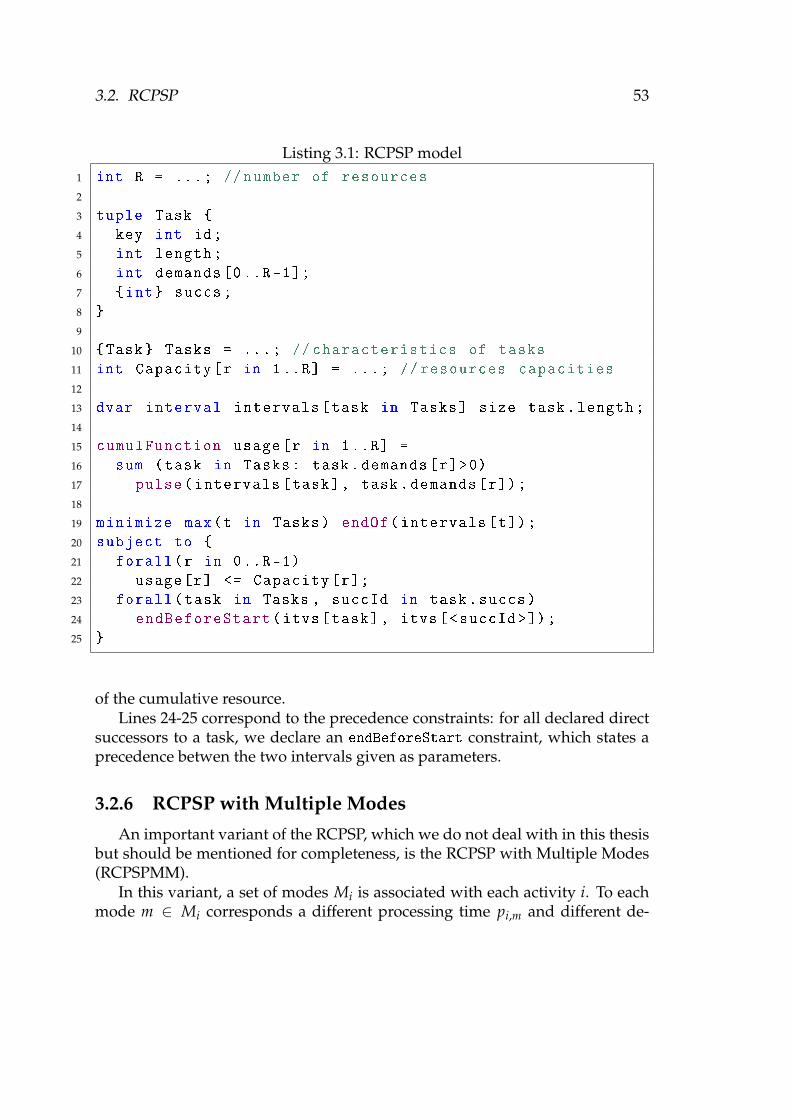
3.2. RCPSP 53
Listing 3.1: RCPSP model1 int R = ...; // number of resources
2
3 tuple Task
4 key int id;
5 int length;
6 int demands [0..R-1];
7 int succs;
8
9
10 Task Tasks = ...; // characteristics of tasks
11 int Capacity[r in 1..R] = ...; // resources capacities
12
13 dvar interval intervals[task in Tasks] size task.length;
14
15 cumulFunction usage[r in 1..R] =
16 sum (task in Tasks: task.demands[r]>0)
17 pulse(intervals[task], task.demands[r]);
18
19 minimize max(t in Tasks) endOf(intervals[t]);
20 subject to
21 forall(r in 0..R-1)
22 usage[r] <= Capacity[r];
23 forall(task in Tasks , succId in task.succs)
24 endBeforeStart(itvs[task], itvs[<succId >]);
25
of the cumulative resource.Lines 24-25 correspond to the precedence constraints: for all declared direct
successors to a task, we declare an endBeforeStart constraint, which states aprecedence betwen the two intervals given as parameters.
3.2.6 RCPSP with Multiple Modes
An important variant of the RCPSP, which we do not deal with in this thesisbut should be mentioned for completeness, is the RCPSP with Multiple Modes(RCPSPMM).
In this variant, a set of modes Mi is associated with each activity i. To eachmode m ∈ Mi corresponds a different processing time pi,m and different de-

54 CHAPTER 3. THE CUMULATIVE CONSTRAINT
mands di,r,m on the cumulative resources. This is used to model the frequentsituations in which different processes or machines can be used to obtain thesame result, albeit with a different processing time. In addition to setting start-ing dates, the solver must select a mode for each activity.
In CP Optimizer, alternatives can be used to model the RCPSPMM.
3.3 Examples of industrial applications of thecumulative constraint
Since this thesis was prepared in an industrial setting, we wish to presentsome concrete examples of the usage of the cumulative constraint, to show howversatile it is. In our experience, more than half of all scheduling models involvea cumulative constraint. Our goal is to represent the variety of its uses, bothfrom an application and a modelization standpoint.
3.3.1 Exclusive zones
Many areas in an aircraft under construction are cramped and can only acco-modate a limited number of workers, or are supported by scaffolding and havesevere weight limits. Exclusive zones are extensively used in aircraft manufac-turing to account for these restrictions. The principle is to divide the aircraftinto zones, and to limit the number of people working simultaneously in a zone(or a union of zones) using a cumulative constraint.
Figure 3.4 shows an example of splitting the forward section of an aircraftinto different exclusive zones, and the associated constraints.
The cumulative resource is often used to model such volume limitations inthe case of processing several items at once, for example in chemical reactors orin ovens, in semiconductor manufacturing.
3.3.2 Workforce scheduling
A common application of scheduling is the building of rosters. Differenttasks have to be assigned to different employees. Each task requires a certainskill, and employees each have a set of skills. The easiest way of modeling thiswith CP Optimizer is to have an interval for each task ti, and to create optionaltasks tij for each task ti and each employee j which has the skills to completetask ti. Two types of constraints are then used: an alternative from each maintask ti to the subtasks tij, which ensures that the task will be assigned to exactlyone employee, and a no-overlap constraint for each worker j on all the tasks tij

3.3. EXAMPLES OF INDUSTRIAL APPLICATIONS OF THE CUMULATIVECONSTRAINT 55
UL UC UR
ML MC MR
LL LC LR
Zones Max number of peopleUL 1UC 1UR 1ML 1MC 2MR 1LL 1LC 2LR 1
UL+UC+UR 2ML+MC 2MC+MR 2
UL+UC+UR+LL+LC+LR 3LL+LC+LR 2
Figure 3.4: Exclusive zones in the forward section of an aircraft
potentially assigned to that worker. This model is shown on Figure 3.5 and inListing 3.2.
It is very helpful here to add a redundant cumulative constraint for eachskill. These cumulative constraints will relax the exact assignment of tasks toworkers, but they will have a more global view of all the tasks sharing certainworkers. This will enable them to make deductions that the no-overlap con-straints would have missed. For each skill, we thus define a new cumulativeconstraint. Its capacity is the number of workers having that skill, and the de-

56 CHAPTER 3. THE CUMULATIVE CONSTRAINT
t
Skills
W3
W2
W1
t1 t3 t4t2ALT ALT ALT ALT
Figure 3.5: Workforce scheduling
mand of each task ti on the constraint is 1 if it requires that skill, 0 otherwise, asshown in Listing 3.3.
Using a cumulative resource as an approximation for identical machines isoften a wise and efficient practice for non-critical parts of a model.
3.3.3 Long-term capacity planning
In supply chain management, capacity planning consists in matching theresource availabilities and customer demands for the products of a company. Ingeneral, the long term strategy of the company is at stake.
This problem is generally modeled as a linear problem by assimilating theproduction as a cumul of demands over a small number of fixed time buckets.The expected demands come from strategic forecasts, the time horizon is huge,typically in years, and the buckets duration is long as well, typically one month.The objective is then to choose which resources to use for the production, andto compute an approximate production date.
Nevertheless, the long duration time buckets relaxation is not precise enoughfor some cases. This is for example the case when precedence constraints be-tween demands, or costs in case of early or late delivery, are key factors. Itprevents from safely aggregating the demands in buckets and requires a con-tinuous time definition. If we suppose that the relaxation of the productionsystem as cumulative resources is still valid, the core problem is then an RCPSP(eventually an RCPSPMM) with a huge number of tasks, typically up to onemillion, and a large set of cumulative resources, typically in the hundreds.
3.3.4 Berth allocation
This example is an original, though not uncommon, application of the cu-mulative constraint to a geometric problem. A commercial port has a linearquay of length L. Ships can dock anywhere along the quay, but their berthinglocations obviously cannot overlap, see Figure 3.6. The ships are indexed from

3.3. EXAMPLES OF INDUSTRIAL APPLICATIONS OF THE CUMULATIVECONSTRAINT 57
Listing 3.2: Workforce scheduling model1 int n = ...; // number of tasks
2 int w = ...; // number of workers
3 int s = ...; // number of skills
4
5 int taskType[i in 1..n] = ...; //skill needed by a task
6 int skillsWorker [1..w][1..s] = ...; //1 if worker has
the skill , 0 otherwise
7 int skillAvailability[k in 1..s] = sum(j in 1..w)
skillsWorker[j][s];
8
9 dvar interval tasks[1..n];
10 dvar interval assignedTasks [1..n][1..w] optional;
11
12 constraints
13 forall(i in 1..n)
14 alternative(tasks[i],all(j in 1..w: skillsWorker[j][
taskType[i]] == 1) assignedTasks[i][j]);
15 forall(j in 1..w: skillsWorker[j][ taskType[i]] == 0)
16 !presenceOf(assignedTasks[i][j]);
17
18 forall(j in 1..w)
19 noOverlap(all(i in 1..n) assignedTasks[i][j]);
20
21 forall(k in 1..s: skillAvailability[k]>0)
22 sum(i in 1..n: taskType[i] == k) pulse(tasks[i], 1) <=
skillAvailability[k];
1 to n. Ship i has a length of li meters. Its arrival time at the port is ai and it mustdepart before time di while spending at least si time units docked. The goal isto find berthing locations and times which prevent the overlaps.
0 L
Figure 3.6: Berth allocation
This problem is a strip-packing problem, if we think of the temporal dimen-

58 CHAPTER 3. THE CUMULATIVE CONSTRAINT
Listing 3.3: Redundant cumulative1 int skillAvailability[k in 1..s] = sum(j in 1..w)
skillsWorker[j][s];
2
3 constraints
4 forall(k in 1..s)
5 sum(i in 1..n: taskType[i]==k) pulse(tasks[i],1) <=
skillAvailability[k];
6
sion as the infinite dimension in a strip-packing problem. Since the cumulativeconstraint is a very strong relaxation of bidimensional packing problems, all themore so when there is a “thin” dimension, we can get a solution to the originalproblem which is almost always feasible just by modeling it as a cumulativeproblem, as shown in Listing 3.4.
Listing 3.4: Berth allocation model1 int n = ...; // number of docking events
2 int L = ...; // length of the quay
3
4 dvar interval ship[i in 1..n] ...;
5 cumulFunction quayOccupation = sum(i in 1..n) pulse(ship
[i], l[i]);
6
7 constraints
8 forall(i in 1..n)
9 startOf(ship[i]) >= a[i];
10 endOf(ship[i]) <= d[i];
11 lengthOf(ship[i]) >= s[i];
12
13 quayOccupation <= L;
14
In many instances and for all practical purposes, since ships have a largeenough length and only a small number of them can fit on the quay at the sametime in the real-world problem, this model provides an exact relaxation of theoriginal problem.

3.3. EXAMPLES OF INDUSTRIAL APPLICATIONS OF THE CUMULATIVECONSTRAINT 59
The principle of using a cumulative resource to model a strip packing prob-lem with a thin dimension applies to vehicle loading problems such as truck ortrain loading. The idea consists in using the temporal dimension of the cumu-lative resource to model the length of the vehicle, as shown on Figure 3.7.
t
Figure 3.7: Truck loading
3.3.5 Balancing production load
In CP Optimizer, the demand of a task can also be a decision variable, andnot only a data of the problem. One example of a use case is in balancing aproduction load.
In many industrial problems, the real objective is to balance the productionas evenly as possible, which is not easy to express as an objective function inan optimization model. A way of accomplishing this is to minimize the peakutilization of the resources. In this example, a dummy task of variable demandD is added to the cumulative constraint and the objective is to maximize D, asshown in Figure 3.8 and Listing 3.5.
Many variants of this idea can be used to balance a load, such as having adummy task per work shift.
tA1
A2
A3 A4 A5
A6
A7
dummy D
C
Figure 3.8: Balancing production load

60 CHAPTER 3. THE CUMULATIVE CONSTRAINT
Listing 3.5: Balancing production load1 int n = ...; // number of tasks
2 int C = ...; // cumulative capacity
3
4 dvar interval A[i in 1..n] ...;
5 dvar interval dummy ...;
6 cumulFunction f = pulse(dummy , 0, C) + sum(i in 1..n)
pulse(A[i], 1);
7
8 maximize heightAtStart(dummy , f);
9 constraints
10 f <= C;
11
3.3.6 Batching
Another type of constraint, related to the cumulative constraint as definedpreviously, is the alwaysIn constraint. We do not deal with the algorithmic as-pects of the alwaysIn constraint in this thesis, but mention it here for compre-hensiveness. alwaysIn( f , a, hmin, hmax) states that during the execution intervalof activity a, the cumulative function f , representing the sum of the demands ofthe tasks being executed at a certain point in time, must always be at a level inthe range [hmin, hmax].
In the following example which is sometimes encountered in process schedul-ing models (OPL code in Listing 3.6 and illustration in Figure 3.9), the alwaysInconstraint is used to locate production periods, in order to fit maintenance tasksbetween those periods. The production tasks take place during the Ai inter-vals. We want a Wj interval to be present exactly whenever an Ai interval ispresent. To this end, the constraint alwaysIn(CW, A[i], 1, 1) ensures thatexactly one Wj interval is present whenever an Ai interval is present. Theconstraint alwaysIn(CA, W[i], 1, n) ensures that at least one Ai interval ispresent whenever a Wj interval is present, so that no Wj interval is present whenno Ai interval is present.
A natural extension of the cumulative resource is the “reservoir”, which is asuccession both of filling and emptying events, for which we have a minimumlevel constraint (in general 0) and a maximum level constraint (the reservoirvolume).
In this thesis, we will not deal with negative demands nor minimum levelsin cumulative resources.

3.4. CUMULATIVE PROPAGATION 61
0
1
n
A4
A6
A6 A5 A3
A1
A2
0
1W1 W2 W3
Figure 3.9: Intervals synchronization
Listing 3.6: Intervals synchronization1 int n = ...;
2
3 dvar interval A[i in 1..n] ...;
4 cumulFunction CA = sum(i in 1..n) pulse(A[i], 1);
5 dvar interval W[i in 1..n] optional in 1.. horizon;
6 cumulFunction CW = sum(i in 1..n) pulse(W[i], 1);
7
8 constraints
9 forall(i in 1..n)
10 alwaysIn(CW, A[i], 1, 1);
11 alwaysIn(CA, W[i], 1, n);
12
13 forall(i in 1..n-1)
14 endBeforeStart(W[i], W[i+1]);
15
16
3.4 Cumulative propagation
We describe in this section the most common propagations for the Cumula-tive constraint. These propagations only take into account the current boundsfor the start and end times of the different activities, except for the PrecedenceEnergy which also takes precedence relationships into account. Most of thesepropagations rely on the notion of Energy Bound, defined above in Section 3.1.

62 CHAPTER 3. THE CUMULATIVE CONSTRAINT
The general principle is to select a set of activities, select a time interval wherethese activities should be scheduled, and move an activity if the total energy ofthe activities exceeds the available energy in the window.
There are dominance relationships between these propagations, in the sensethat the deductions made by some of them are subsubmed by the deductionsmade by another one with a higher algorithmic complexity. In particular, En-ergy Reasoning is stronger than the Edge-Finders. It is also stronger than theTimetable. It is worth noting though that Energy Reasoning and Not-First, Not-Last are incomparable and can both make deductions that the other cannot.
3.4.1 Timetable
The timetable propagation was introduced in [AB93]. A lot of improvementhas since been made on this topic and exists unpublished in the community. Thetimetable has a quadratic worst-case complexity but its amortized complexityis linear. In spite of its relative propagation weakness, its low complexity makesit the basis of propagating the cumulative constraint.
The timetable amounts to maintaining arc-B-consistency on the equationfrom Definition 1 which defines a satisfied cumulative resource.
The principle is to maintain a so-called resource histogram, recording foreach point in time the minimum amount of resource consumption: first we com-pute for each task its compulsory part, that is
Mi(t) ,
ci if lsti ≤ t < eeti
0 otherwise
We accumulate for each time point the compulsory parts of all tasks:
U(t) , ∑i
Mi(t) = ∑i∈J1,nK:lsti≤t<eeti
ci
Several deductions can be made with this histogram:
• If ∃t/U(t) > C, then we know that the current problem has no solutionand the search must backtrack.
• If for a particular task Ai, ∃t0/ max(lsti, eeti) ≤ t0 < leti, U(t0)−Mi(t0) +ci > C, then Ai cannot end after t0, otherwise the resource would be over-consumed. leti can then be updated to t0. A symmetric rule exists forupdating the start times.

3.4. CUMULATIVE PROPAGATION 63
In addition to its low complexity, a major advantage of the timetable is that itis easily extendable. It can easily support extensions such as reservoirs (nega-tive demands and minimum level constraints on a cumulative), as well as thejoint propagation of other resources such as state functions with transition time,without incurring a performance penalty.
The implementation in CP Optimizer is fully incremental with respect tochanges to the interval variables domains.
3.4.2 Disjunctive
If the sum of the demands of two activities Ai and Aj exceeds the capacityof the cumulative, they cannot overlap in time, so one of them must precede theother. The disjunctive constraint maintains arc-consistency on the formula:
[ci + cj ≤ C
]∨[Ai → Aj
]∨[Aj → Ai
]
This constraint can be propagated on all activities with a O(n log n) complex-ity, as explained in [Vil04]. This propagation is surprisingly powerful in prac-tice, since many instances of cumulative problems exhibits tasks which cannotoverlap.
3.4.3 Edge Finding and derivatives
The Edge-Finding family of propagation techniques reason about the orderof execution of activities. Specifically, these algorithms determine if a givenactivity Ai must execute before (or after) a set of activities Ω. Two types of in-formations can be drawn from this: new precedence relations, sometimes calledimplicit precedences or “edges”, and more importantly new bounds on the ex-ecution dates of activities.
The general principle is to check if the total energy of a set of activities Ω fitsin the available energy for Ω, otherwise a conflict is detected:
C(letΩ − estΩ) < eΩ ⇒ fail.
There exists a breadth of Edge-Finder variants, with different propagationpower versus algorithmic complexity trade-offs, and research is very active inthis area. We present the most common versions.
Edge-Finder The original cumulative Edge-Finder was introduced in [Nui94].For Ai /∈ Ω, if
C(letΩ − estΩ∪Ai) < eΩ∪Ai,

64 CHAPTER 3. THE CUMULATIVE CONSTRAINT
then Ai must end after lctΩ. Indeed, the previous condition is satisfied if theenergy overflows when Ai is forced to finish no later than letΩ.
The original complexity of this propagation was O(n2) where n is the num-ber of activities, and it was improved in [Vil09a] to O(kn log n), where k is thenumber of different demands of the activities, thanks to a new data structurecalled Θ-tree.
Extended Edge-Finder The Extended Edge-Finder was also introduced in [Nui94].Instead of considering the [estΩ∪Ai, letΩ) window as previously, only the win-dow [estΩ, letΩ) is now considered and only the part of the energy of Ai whichnecessarily falls into this window is taken into account.
The full propagation condition is thus, for Ai /∈ Ω and esti ≤ estΩ < eeti, if
C(letΩ − estΩ) < eΩ + ci(eeti − estΩ),
then Ai must end after lctΩ.The original complexity of this propagation was O(n3), and it was improved
in [MVH08] to O(kn2).
Timetable Edge-Finder The Timetable Edge-Finder was introduced in [Vil11],and combines the Timetable propagation with the Edge-Finder, by also takinginto account the timetable in the overflow condition.
We defined above in Subsection 3.4.1 the U(t) function, which sums themandatory energy of all tasks at time t.
We can thus improve the overload checking rule by adding the energy fromthe timetable:
C(letΩ − estΩ) < eΩ +letΩ
∑t=estΩ
U(t)⇒ fail.
Depending on the relative positions of Ai and Ω, we can add to this equationthe amount of energy of Ai that necessarily falls in the [estΩ, letΩ) window andis not yet taken into account in the timetable to obtain an adjustment rule. Thecomplexity of this propagation is O(n2).
3.4.4 Not-First, Not-Last
The Not-First, Not-Last propagation was originally introduced in [Nui94]. Itgives necessary conditions under which an activity Ai has to be scheduled afterat least one activity (not-first) or before at least one activity (not-last) of a set Ωof activities. This is complementary to edge-finding.

3.4. CUMULATIVE PROPAGATION 65
We now describe the Not-First rule. The Not-Last rule is similar.For a set of activities Ω and an activity Ai /∈ Ω, if
estΩ ≤ esti < minj∈Ω
eetj, and
eΩ + ci(min(eeti, letΩ)− estΩ) > C(letΩ − estΩ),
then Ai must start after minj∈Ω eetj and esti can be updated.Indeed, if we force activity Ai to start at its earliest start time, then no activity
of Ω can be completed before Ai is started, since esti < minj∈Ω eetj. Thus anenergy ci(esti − estΩ) is occupied by no activity before Ai starts, as shown ingreen on Figure 3.10.
The sum of the energy of the activities in Ω∪Ai on the window [estΩ, letΩ)is thus eΩ + ci(min(eeti, letΩ)− esti)+ ci(esti− estΩ), which overflows the avail-able energy.
estΩ letΩminj∈Ω
eetjesti eeti
Ai
Ω
Figure 3.10: Not-First, Not-Last
We can thus deduce that:
esti ≥ max
Ω⊆A1,...,An/
Ai /∈ ΩestΩ ≤ esti < minj∈Ω eetj
eΩ + ci(min(eeti, letΩ)− estΩ) > C(letΩ − estΩ)
minj∈Ω
eetj
The original complexity of propagating this condition on all tasks was O(n3).It was improved to O(n2 log n) in [SW10].

66 CHAPTER 3. THE CUMULATIVE CONSTRAINT
3.4.5 Energy Reasoning
The energy reasoning was originally introduced in [EL90]. It consists in fix-ing a time window, and accumulating for all the the tasks the minimum energywithin the time window. The propagation is triggered when an overflow isdetected. This propagation is extremely powerful and subsumes several otherpropagations (notably timetabling and edge-finding). But its original computa-tional complexity of O(n3) made it unusable in practice. [EL90, BPN01].
The energy reasoning has seen much interest and several improvementsin the recent years, notably in a series of two articles [DP13, DP14] in whichthe constant factor of its complexity was divided by seven, and in techniquesaiming at using machine learning to predict cases when running the expensiveO(n3) Energy Reasoning propagator will be beneficial, so as to use this propa-gation sparingly [VCLSo14].
As part of this doctoral work, we developed a new propagation algorithmwith a complexity of O(n2 log n) [Bon16], making this propagation useful in ahigher number of cases.
We do not detail this propagation here, since it will be extensively coveredin Chapter 5.
3.4.6 Energy Precedence
The energy precedence propagation, introduced in [Lab03a], is different fromthe previous propagations in that it combines information coming from the tem-poral network (precedence constraints) with the information on the cumulativeconstraint and the current domains of the intervals. This propagation is es-pecially useful when used in combination with a precedence-based search (abranching scheme which adds precedence constraints to the model).
The energy precedence ensures that the cumulative resource provides enoughenergy for all the predecessors of a task to fit before that task can start. Moreformally, for each subset Ω of predecessors of a task Ai, the earliest start time ofa task in Ω plus a lower bound on the running time of all the tasks in Ω providesa lower bound on the earliest start time of Ai:
∀Ω ⊆ j ∈ J1, nK : Aj → Ai, esti ≥ estΩ +⌈ eΩ
C
⌉
There exists a symmetric rule with the successors and latest end time of i.Since subsets Ω of the form j ∈ J1, nK : Aj → Ai, estj ≥ t dominate the
other subsets for this propagation, and there are only p of them where p is themaximal number of predecessors of a given activity in the temporal network(p < n), the energy precedence can be propagated with a worst-time complexityO(n(p + log n)).

3.5. MIP FORMULATIONS 67
3.5 MIP formulations
Numerous MIP formulations have been proposed for the RCPSP. Neverthe-less, a major difficulty in coming up with good formulations is that the cumu-lative constraint is deeply non-linear with respect to the dates of the activities.In other words, it is very difficult to express the temporal and cumulative con-straints jointly using linear inequalities.
This requires compromises on the size of the formulation and the quality ofthe linear relaxation, which are done by choosing different variables, represent-ing more or less directly the temporal and cumulative constraints, and thus bydifferent linearizations, more or less precise and more or less compact. Never-theless, there is no good compact linearization and we have to choose betweeneither a weak approximation or a pseudo-polynomial model. For this reason,only small instances have been solved to optimality, or instances with addi-tional properties that could be exploited in the MIP model. Additionally, thelinear relaxations of these formulations are generally weak.
The fundamental notion in most of these formulations and attempts at lin-earizing the cumulative constraint is that of antichains (set of activities whichare incomparable in the precedence relation and can a priori be scheduled si-multaneously).
Following Queyranne and Schulz’s [QS94] classification of MIP formula-tions, we will group them hereafter by the type of decision variables used.
Time indexed formulations Time indexed formulations were introduced in[PWW69]. They are, perhaps surprisingly, the most commonly used MIP for-mulations for the RCPSP, owing to their simplicity, in spite of their poor prac-tical performance on most instances. The basic principle (Discrete Time for-mulation) is to divide the scheduling horizon H into unit time slots and to usetime-indexed binary variables: for any activity i and time t ∈ [0, T], xit = 1if activity i starts at time t, 0 otherwise. With these variables, the precedence
constraint from i to j is expressed asH
∑t=0
txjt −H
∑t=0
txit ≥ pi and the cumulative
constraint asn
∑i=1
ci
t
∑τ=t−pi+1
xiτ ≤ C for all times t ∈ [0, H − 1].
In the Disaggregated Discrete Time formulation, the precedence constraints
are desagregated intot−pi
∑τ=0
xiτ −t
∑τ=0
xjτ ≥ 0 for all times t ∈ [0, H − 1] as in-
troduced in [CAVT87]. We obtain a stronger continuous relaxation and betterlower bounds. Moreover, if the cumulative constraints are dualized with a La-

68 CHAPTER 3. THE CUMULATIVE CONSTRAINT
grangian relaxation, the remaining constraint matrix is totally unimodular. Thisfact was used in [MSSU03] to solve the remaining problem with a maximumflow algorithm.
An even stronger linear relaxation can be obtained by replacing the cumu-lative constraint as expressed above by its Dantzig-Wolfe decomposition, usingantichains. More specifically, we call P the set of antichains P. Pi is the set ofantichains containing activity i. The decision variable yPt is equal to 1 if an-tichain P is being executed at time t, 0 otherwise. The cumulative constraint isnow expressed as:
∀i ∈ [1, n], ∑P∈Pi
∑t∈[0,H−1]
yPt = pi,
so that enough antichains are available to execute all of activity i.
∀t ∈ [0, H − 1], ∑P∈P
yPt ≤ 1,
to schedule only one antichain per time slot.
∀i ∈ [1, n], ∀t ∈ [0, H − 1], xit − ∑P∈Pi
yPt − ∑P∈Pi
yP,t−1 ≥ 0,
to synchronize the start date of i with the first use of an element of Pi.This formulation was introduced in [MMRB98]. It was further improved
with constraint propagation and specific cutting planes in [BK00, BD04].All these time indexed formulations are pseudo-polynomial in H.
Continous time formulations These formulations are based on two familiesof variables: n continuous variables Si representing the starting time of eachactivity and n2 binary sequencing variables xij between all pairs of activities,representing precedences between activities: xij = 1 if activity j does not startbefore activity i is completed, and 0 otherwise.
The basic constraints of these formulations enforce the asymmetry and thetriangle inequality of the precedence relation: xij + xji ≤ 1 and xij + xjh − xih ≤1, , and the precedence relationship from i to j with a big-M: Sj − Si −Mxij ≥pi −M.
The first formulation based on these variables [AVOTG93] relies on the con-cept of forbidden sets. A forbidden set F is a set of activities which cannot bescheduled simultaneously because the sum of their demands would exceed thecumulative capacity, so for any forbidden set F, we add a constraint to forcea precedence between two activities: ∑i,j⊆F xij ≥ 1. There is is an exponen-tial number of forbidden sets in general, so this formulation cannot be used inpractice.
A second formulation based on the concept of resource flow was proposedin [AMR03] to obtain a more compact formulation. The principle is to indicate

3.6. LP-BASED STRENGTHENING OF THE CUMULATIVE CONSTRAINT69
the quantity of cumulative resource made available for activity j when activ-ity i finishes. Two families of constraints are then added to the model to ex-press that the total incoming and outgoing flow to an activity must match itsdemand. Two dummy activities are placed at the beginning and end of theschedule to provide and capture all the capacity. This formulation has O(n2)binary variables, O(rn2) continuous variables and O(rn2 + n3) constraints, so itis reasonably compact. Note moreover that the model size does not depend onthe scheduling horizon H.
Event-based formulations Event-based formulations, introduced in [KALM11],are based on the fact that an optimal solution to an RCPSP always exists wherethe start time of any activity coincides with the end time of another activity,or with the scheduling origin (a property which was already exploited implic-itly by the flow formulation above), so only n events have to be scheduled. Wethus have n continuous variables to represent the events dates, with an orderingconstraint to break symmetry.
Two families of formulations exist, depending on how the activities are con-nected to the events. In the Start/End formulations, we have two binary vari-ables for each activity/event pair: xie = 1 if activity i starts at event e and 0otherwise, and yie = 1 if activity i ends at event e and 0 otherwise. In theOn/Off formulations, we only use one binary variable for each activity/eventpair: zie = 1 if activity i starts or is still being processed at event e.
These formulations both have O(n2) binary variables, O(n) continuous vari-ables and O(n3 + n(p + r)) constraints where p is the number of precedenceconstraints. The linear relaxation quality is quite poor, though.
3.6 LP-based strengthening of the cumulativeconstraint
Many methods have been developed to calculate lower bounds on the makespanof RCPSP. As we will explain in much more detail in Chapter 4, we noticedas part of the work done in preparing this thesis that many of these meth-ods, notably several of these relying on a linear programming formulation, aswell as the new cumulative strengthening method that we present in Chap-ter 4, provide naturally, in addition to a lower bound, a redundant cumulativeconstraint. Redundant means that we do not lose a feasible solutions but ob-tain different demands, which can possibly be exploited to compute strongerpropagations. This is another example of the integration of various algorithmicmethods through Constraint Programming.

70 CHAPTER 3. THE CUMULATIVE CONSTRAINT
In these methods, we often first relax the RCPSP into a CuSP, that is weabandon the precedence constraints and keep only one cumulative constraint.
The first method known to us to introduce a reformulation of the cumulativeconstraint was based on Dual Feasible Functions. A good survey was publishedin [CAdC10]. DFF are functions that map the original demands to demands ina new cumulative functions, in such a way that no feasible solution is lost. Inthis line of research, particular classes of functions which satisfied this property,as well as a branch and bound algorithm to generate them all were exhibited.There was no reformulation giving a different demand to each activity, or takinginto account special cases, such as very long activities. We are also not aware ofDFF being used to strengthen propagation, but only to compute global bounds.
As for the methods based on linear programming, those computing a LinearLower Bound, such as in [CN00], can be used to compute a reformulation aswell. Indeed, studying the dual of the linear program immediately yields aredundant cumulative function.
Other methods based on linear formulations exist and could be used to com-pute a form of cumulative strengthening, such as [MMRB98, BK00, CN03], butthose formulations are time-indexed and would yield a complex reformulationwith a variable demand profile. The computations would probably be too heavyfor this to be of any practical use.
Note that many other techniques to compute LB which do not yield strenght-ening exist, but we do not mention them here. Information about them can befound in the survey [NAB+06], in Section 3.7 of [BK12], or in [Art16].
The Cumulative Strengthening as we introduce it in Chapter 4 is much strongerthan Dual Feasible Functions while being much cheaper to compute than theformulations based on linear programming that we mentioned above.
3.7 Conflict-based search
The most effective way to do this is to look for a conflict as high up as possi-ble in the search tree, and that for two purposes. First, the higher the conflict inthe tree, the largest the volume of the search space it cuts. Second, learn a newconstraint (no-good) from this conflict, in order not to direct the search anymorein this area of the search space.
For very hard feasibility problems or when trying to prove that the solutionobtained is optimal (so-called exact method), we must explore the entire searchspace.
Some historical approaches use RCPSP-specific structures, but this is nolonger the case in the latter approaches which memorize very simple decisionsand operate in a much more general framework than the RCPSP.

3.7. CONFLICT-BASED SEARCH 71
The first such approach was introduced in [DH97] and relies on cutsets (setsof activities whose predecessors have all been scheduled already). If the searchreaches a cutset which has already been processed, we can reuse the result fromthat earlier search which has been saved. This method was for a decade thebest way of exploring the whole search space of an RCPSP and proving lowerbounds.
Minimal Critical Sets were introduced in [Lab05]. They are sets of activitieswhich violate a cumulative constraint, and thus cannot be scheduled simulta-neously, so there must be a precedence between (at least) two of them. TheMCS-based search thus branches on possible precedences which break MCS.
Yet another approach was introduced in [SFSW10] and consists in model-ing the RCPSP as a SAT problem, using the TTEF propagation to enforce thecumulative constraint. The main idea here is to use the native clause learn-ing mechanism of the SAT solver, using so-called TTEF explanations: when aconflict is detected by the TTEF, a clause is generated and added to the SATformulation. The basic decisions in this formulation consists of inequalities be-tween start dates of tasks and times. This approach works well for problemswith small time horizons, but because the time is enumerated in the formula-tion, this approach doesn’t scale to realistic time horizons.
The last approach to date is the Failure Directed Search, which we explain inmore detail in Subsection 2.5.3.4.
As a general remark, these techniques (and all decision making techniquesfor scheduling problems, such as branching heuristics, local search techniques,and propagations) fall into two categories, depending on whether they raise aprecedence between two activities or they set a temporal bound on the start orend time of an activity.
It seems that decisions on precedences have less impact than decisions ontimes, at least to find a solution, and that decisions on dates scale better as well.This can be seen with the extreme example of assuming that we have a perfectbranching heuristic and that we will find the optimal solution by always takingthe left branch at each node: with a chronological branching rule such as Set-Times, only n decisions have to be taken in this case, while n2 decisions have tobe taken if we want to raise all precedences.
If the goal is to prove optimality, the best approach is less clear. Experimentswith the Failure Directed Search algorithm show that the Set-Times rules worksa bit better than precedence raising, but the reason is unclear, and this observa-tion might just come from lack of research in this direction.
Another reason to prefer taking decisions on dates is that all decision-takingmethods in a constraint programming engine have to work well together, andthat propagations of the cumulative constraints on precedences have not been

72 CHAPTER 3. THE CUMULATIVE CONSTRAINT
developed as much as propagations on dates.As far as we know, no research has been done yet on trying to record prece-
dence disjonctions of small cardinality as no-goods. This research directionmight yield interesting results.
3.8 List schedulingThe RCPSP is often referred to as one of the most intractable problems in
Operations Research, since even very small instances can not be solved to opti-mality with the current technology. To circumvent this limitation of exact meth-ods, numerous RCPSP-specific heuristics have been developed. A good surveyof the different techniques can be found in [HK00], but detailed experimentsand comparisons reveal that all good heuristics and local search techniques boildown to list scheduling.
The general principle of list scheduling (sometimes also called ScheduleGeneration Schemes) consists in representing a solution in the form of a total or-dering of the activities (list), which is then transformed into a schedule througha decoding procedure specific to the particular heuristic.
An example of a decoding procedure is the Earliest Start Schedule, whichconsists in taking the first activity in the list, scheduling it at the earliest datepossible which does not conflict with an already scheduled activity, and repeat-ing these steps until the list is empty. This particular decoding procedure hasthe convenient property that for an RCPSP with a regular objective function, alist of all activities always exists such that the procedure Earliest Start Scheduleprovides an optimal schedule. Many other decoding procedures are availablein the literature.
On the other hand, this heuristic works poorly when no good decoding pro-cedure exists for the particular constraints or objective of the problem, for ex-ample when there are many implicit precedences, or if the objective is irregular.
An efficient improvement of list scheduling procedures is called Forward-Backward Improvement. After decoding a given list, a new list is created byranking the activities in the order of decreasing completion times. This list isdecoded into a backward schedule, and the whole procedure is repeated untilno new schedules are created. The best schedule which appeared in the courseof the process is output.

Chapter 4
Cumulative Strengthening
As mentioned above in Section 3.6, several methods of computing lowerbounds on the makespan of an RCPSP, especially those based on the energybound, can be extended to provide a redundant cumulative constraint as well.
In this chapter, which was already published as [BB17a], we show how toconstruct redundant cumulative constraints.
4.1 Introduction
The objective of this work is thus not to give a new filtering algorithm, butto improve all the reasonings based on the notion of energy, which will auto-matically improve the existing filtering algorithms which rely on this notion,notably timetabling and edge-finding. See for example Figure 4.1, which givesa possible reformulation for the instance of Figure 3.1: the energy bound is in-creased from 9.75 to 11.5, and this will help the filtering algorithms adjust thetime bounds for this instance.
C = 4
t
Figure 4.1: Reformulation of the instance of Figure 3.1. Energy bound: 11.5.
The reformulation of cumulative constraints that we introduce in this chap-ter is such that all valid schedules remain valid for the reformulated constraint,but we now have a guarantee that the energy lower bound matches the makespanof the preemptive relaxation. The preemptive relaxation of a cumulative resource
73

74 CHAPTER 4. CUMULATIVE STRENGTHENING
problem is a solution which satisfies the cumulative constraints but enablestasks to be interrupted and restarted later (compared to a non-preemptive sched-ule where a task of length p must run uninterrupted from its starting time t untilt + p). These reformulations are relatively cheap to compute (after a precompu-tation which does not depend on the instance) and they provide a significantimprovement for all algorithms which rely on energy reasonings. In our exper-iments, we used them within an edge-finding algorithm.
Let us start by studying two small examples for a resource of capacity C = 3,to get an idea of the spirit of these reformulations:
Since on such a resource a task of demand 3 cannot run in parallel with anyother task, it can occupy the whole resource. Moreover, since a task of demand2 cannot run in parallel with another task of demand 2, a valid bound on themakespan of such an instance is the sum of the lengths of tasks of demand 2 and3. Hence, a valid reformulation for a resource of capacity C = 3 is to discardtasks of demand 1, and to increase the demand of tasks of original demand 2,so that they now occupy the full capacity of the resource. See Figure 4.2 for anexample where this reformulation increases the energy bound from 7.33 to 8.
3 3
Figure 4.2: Energy bound increased from 7.33 to 8.
Again for a resource of capacity C = 3, we notice that the longest task ofdemand 1 cannot run in parallel with any task of demand 3. So a valid lowerbound on the makespan is the sum of the lengths of tasks of demand 3, plusthe length of the longest task of demand 1. Hence, a valid reformulation for aresource of capacity C = 3 is to discard tasks of demands 1 and 2, except for thelongest one of demand 1, and to increase the demand of that task so that it nowoccupies all of the capacity of the resource. See Fig. 4.3 for an example wherethis reformulation increases the energy bound from 9 to 10.
3 3
Figure 4.3: Energy bound increased from 9 to 10.
In the rest of this chapter, we will introduce a new method to compute lowerbounds for the cumulative resource problem. We will show that it also yields anew, valid, cumulative constraint which can itself be passed to existing filteringalgorithms for further propagation. We will then show that after a precomputa-tion phase which is independent from the instance, computing this redundant

4.2. A COMPACT LP FOR PREEMPTIVE CUMULATIVE SCHEDULING 75
constraint for a given problem can be done very effectively. Then we will pro-vide some experimental results. A similar approach was introduced in [CN07]under the name of dual feasible functions. We will show that our approachgeneralizes and supersedes the dual feasible functions based redundant con-straints.
4.2 A compact LP for preemptive cumulativescheduling
4
0001
1010
2100
0200
4000
P1P2P3P4
Figure 4.4: The five possible task configurations on a cumulative of capacityC=4.
4
0001
1010
2100
P1P2P3P4
Figure 4.5: The three task configurations used to build the reformulation ofFigure 3.1.
We are given a discrete cumulative resource of capacity C and a set of tasks,each with a fixed length and demand level. We want to compute a lower boundof the makespan of non-preemptive schedules of the set of tasks on the resource.
We now introduce tasks configurations: a configuration is an integer vectorP of size C such that ∑C
c=1 Pc × c = C. Pc is the number of tasks of demand cin configuration P. Thus, the configurations are exactly the integer partitions of

76 CHAPTER 4. CUMULATIVE STRENGTHENING
C (see Figure 4.4). We denote them P . xP can be interpreted as the time dur-ing which configuration P is run. A configuration indicates a number of tasksfor each demand level which can run at the same time on the cumulative re-source. See Figure 4.5 for an example, where the resource has capacity C = 4:the configuration P = (2, 1, 0, 0) corresponds to the possibility of running 2tasks of demand 1 and 1 task of demand 2 simultaneously on the resource. An-other possible configuration could be P = (4, 0, 0, 0), corresponding to running4 tasks of demand 1 simultaneously.
Note that these are demands configurations, not tasks configurations as of-ten seen with configuration LPs.
A key idea in our approach is the use of non-superposition constraints: a taskcannot run in parallel of itself, so it can only use one slot on a given configura-tion. Generalizing this idea, any j tasks of demand c can only occupy up to jslots of demand c on a configuration, otherwise there would be at least a taskoccupying two slots on a configuration. This remark justifies the second set ofconstraints in the linear program below, called non-superposition constraints.
For each demand c ≤ C, we call sc the sum of the lengths of tasks of demandc, and for 1 ≤ j ≤ bC
c c − 1, sc,j the sum of the lengths of the j longest tasks ofdemand c:
∀1 ≤ c ≤ C, sc = ∑i:ci=c
pi
∀1 ≤ c ≤ C, ∀1 ≤ j ≤ bCcc − 1, sc,j = max
I :
|I| = j∀i ∈ I , ci = c
∑i∈I
pi
Given the setP of all combinations of the demands of tasks which can be runat the same time, we can show that the optimal value of the following LP is theminimal makespan for a preemptive schedule which satisfies the cumulativeconstraint:
min ∑P∈P
xP
s.t. ∀c ∈ [1, C] ∑P∈P
PcxP ≥ sc (4.1)
∀c ∈ [1, C], ∀j ∈ [1, bCc c − 1] ∑
P∈Pmin(Pc, j)xP ≥ sc,j (4.2)
∀P ∈ P xP ≥ 0
The first set of constraints, labelled (4.1), states that for each demand level c,the total time allocated on the resource for tasks of demand c should be greaterthan the total length of these tasks. Indeed, Pc is the number of slots for tasks of

4.2. A COMPACT LP FOR PREEMPTIVE CUMULATIVE SCHEDULING 77
demand c on configuration P and xP is the number of times that configurationP is selected. The sum runs over all the configurations.
The second set of constraints, labelled (4.2), are the non-superposition con-straints as introduced above. They ensure that whenever we schedule only jtasks of the same demand level, we take into account at most j occurrences ofthis demand level in each configuration, so that a given task cannot occupymore than its demand in any configuration.
3
Figure 4.6: Example schedule
Let us illustrate this on a simple example: if we have a resource of capacity3, and two tasks, both of demand 1, one of length l and the other of length2l, as illustrated in Figure 4.6, then without the constraints (4.2) the value ofthe best LP solution would be l. Indeed, with C = 3, the configurations areP3 = (3, 0, 0), (1, 1, 0), (0, 0, 1). If we label these configurations respectively 0, 1and 2, the linear program without the non-superposition constraints becomes:
min x0 + x1 + x2
s.t. 3x0 + x1 ≥ 3lx0 ≥ 0x1 ≥ 0x2 ≥ 0
The optimal solution to this program is x0 = l, x1 = 0, x2 = 0, as shown inFigure 4.7.
3
Figure 4.7: Best LP solution without the non-superposition constraints
This is a poor solution since the lower bound is not even as long as thelongest task. Non-superposition constraints prevent this situation from occur-ing. Indeed, the non-superposition constraints in this case are:
x0 ≥ 2l2x0 ≥ 3l
With these additional constraints, the optimal solution is now x0 = 2l, x1 =0, x2 = 0, and we get a lower bound of 2l on the makespan, as expected.
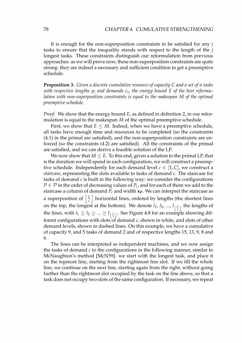
78 CHAPTER 4. CUMULATIVE STRENGTHENING
It is enough for the non-superposition constraints to be satisfied for any jtasks to ensure that the inequality stands with respect to the length of the jlongest tasks. These constraints distinguish our reformulation from previousapproaches: as we will prove now, these non-superposition constraints are quitestrong: they are indeed a necessary and sufficient condition to get a preemptiveschedule.
Proposition 3. Given a discrete cumulative resource of capacity C and a set of n taskswith respective lengths pi and demands ci, the energy bound E of the best reformu-lation with non-superposition constraints is equal to the makespan M of the optimalpreemptive schedule.
Proof. We show that the energy bound E, as defined in definition 2, in our refor-mulation is equal to the makespan M of the optimal preemptive schedule.
First, we show that E ≤ M. Indeed, when we have a preemptive schedule,all tasks have enough time and resources to be completed (so the constraints(4.1) in the primal are satisfied), and the non-superposition constraints are en-forced (so the constraints (4.2) are satisfied). All the constraints of the primalare satisfied, and we can derive a feasible solution of the LP.
We now show that M ≤ E. To this end, given a solution to the primal LP, thatis the duration we will spend in each configuration, we will construct a preemp-tive schedule. Independently for each demand level c ∈ [1, C], we construct astaircase, representing the slots available to tasks of demand c. The staircase fortasks of demand c is built in the following way: we consider the configurationsP ∈ P in the order of decreasing values of Pc, and for each of them we add to thestaircase a column of demand Pc and width xP. We can interpret the staircase asa superposition of
⌊Cc
⌋horizontal lines, ordered by lengths (the shortest lines
on the top, the longest at the bottom). We denote l1, l2, ..., lb Cc c the lengths of
the lines, with l1 ≥ l2 ≥ ... ≥ lb Cc c. See Figure 4.8 for an example showing dif-
ferent configurations with slots of demand c, shown in white, and slots of otherdemand levels, shown in dashed lines. On this example, we have a cumulativeof capacity 9, and 5 tasks of demand 2 and of respective lengths 15, 13, 9, 8 and6.
The lines can be interpreted as independent machines, and we now assignthe tasks of demand c to the configurations in the following manner, similar toMcNaughton’s method [McN59]: we start with the longest task, and place iton the topmost line, starting from the rightmost free slot. If we fill the wholeline, we continue on the next line, starting again from the right, without goingfurther than the rightmost slot occupied by the task on the line above, so that atask does not occupy two slots of the same configuration. If necessary, we repeat

4.2. A COMPACT LP FOR PREEMPTIVE CUMULATIVE SCHEDULING 79
c = 2
C = 9
l1
Figure 4.8: Example of configurations forming a staircase of slots of demand c.
until we can place all the task on the staircase. See Figure 4.9 for an example ofplacing one task. The goal is to preserve a staircase structure after removingthe positions covered by the longest task. We then repeat this process with thefollowing tasks, considered in the order of decreasing lengths. See Figure 4.10for an example, the positions on each line are marked with the number of a task.
1
1
1
c = 2
C = 9
Figure 4.9: Placing one task on the staircase.
5 4 3 2
3 2 1
2 1
1
c = 2
C = 9
Figure 4.10: Preemptive schedule obtained from the staircase.
Let us show that a schedule constructed in this fashion is preemptive. Thereis enough time for all of the tasks to run (constraints (4.1) of the primal), so wewill never have to exceed the capacity of the last line. What remains to prove isthat no job has to be scheduled twice on the same configuration. We will provethis by showing that the staircase invariant ∀k ≤
⌊Cc
⌋, ∑k
j=1 lj ≥ ∑kj=1 pj (where
p1 ≥ p2 ≥ ... ≥ pk) is preserved after placing the longest task as describedabove.

80 CHAPTER 4. CUMULATIVE STRENGTHENING
The case k = 1 is obvious: there is only one line, so there can not be a su-perposition. Otherwise, assume that the invariant is satisfied for the staircase oflengths l. We will place the longest task according to the rule above and showthat the invariant is still satisfied. We define s as the largest integer such thatp1 ∈ [ls+1, ls[. All the lines of index greater than s will be completely filled whenplacing the longest task. We call l′ the length of the staircase lines after placingthe task. There are three cases to distinguish:
If k < s, then ∑kj=1 l′j = ∑k
j=1 lj ≥ ∑kj=1 pj ≥ ∑k
j=1 pj − p1. (The task p1 is notplaced on line k).
If k = s, then ∑kj=1 l′j = ∑k
j=1 lj − (p1− ls+1) = ∑k+1j=1 lj − p1 ≥ ∑k+1
j=1 pj − p1 ≥∑k
j=1 pj − p1. (The task p1 occupies the end of line k).
If k > s, then ∑kj=1 l′j = ∑k
j=1 lj − (p1 − ls+1)−∑kj=s+1(lj − lj+1) = ∑k+1
j=1 lj −p1 ≥ ∑k+1
j=1 pj − p1 ≥ ∑kj=1 pj − p1. (The task p1 occupies all of line k).
This proves that by construction, one can always place the longest task onthe staircase with no superposition, the remaining spots are still staircase-shaped,and the total staircase surface is equal to the total task surface.
Using this construction for each demand level, we can assign locations onthe configurations to tasks independently for the tasks of a given demand. Werepeat this construction for every demand c ∈ [1, C]. Since we do not considertime or precedence constraints, changing the order in which configurations arerun preserves a preemptive schedule.
4.3 ReformulationWe now consider the dual of the previous linear programming formulation:
maxC
∑c=1
schc +
bCc c−1
∑j=1
sc,jhc,j
s.t. ∀P ∈ PC
∑c=1
Pchc +
bCc c−1
∑j=1
min(Pc, j)hc,j
≤ 1
∀c ∈ [1, C] (hc ≥ 0 and ∀j ∈ [1, bCcc − 1] hc,j ≥ 0)
Here we introduce variables hc for each c ∈ [1, C] and hc,j for each c ∈ [1, C]and 1 ≤ j ≤ bC
c c− 1, corresponding to constraints in the primal linear program.The constraints state that all reformulations must remain feasible, and we searchfor the reformulation which gives the largest energy reasoning bound.

4.3. REFORMULATION 81
This dual formulation is particularly interesting in that we can interpret thedual variables as corresponding to demands of a new valid cumulative con-straint, which can be used with all filtering techniques for cumulative con-straints, notably edge-finding. In contrast, previous linear programming ap-proaches to this problem (e.g. [BK00, BD04]) used formulations similar to theprimal formulation above, but did not make use of the new information aboutthe cumulative constraint.
More formally, we can define a new valid cumulative constraint as follows:
Proposition 4. Given a solution to this linear program, if a cumulative resource ofcapacity C is reformulated with a capacity of 1, and that the tasks are ajusted so thatthe demand of the ith longest task of initial demand c becomes hc + ∑j≥i hc,j, then allpreviously feasible schedules are still feasible with the new cumulative resource.
Proof. Schedules which are feasible with the original cumulative resource aresuch that at any point in time, the tasks I being executed satisfy the constraints∑i∈I ci ≤ C, so the set of demands of the tasks being executed is contained inone of the configurations P of P .
We can now rewrite the constraint of the linear program above as follows:
C
∑c=1
Pchc +
bCc c−1
∑j=1
min(Pc, j)hc,j
≤ 1
⇔C
∑c=1
Pc
∑i=1
hc +bC
c c−1
∑j=1
min(Pc,j)
∑i=1
hc,j
≤ 1
⇔C
∑c=1
Pc
∑i=1
hc +Pc
∑i=1
bCc c−1
∑j=i
hc,j
≤ 1
⇔C
∑c=1
Pc
∑i=1
hc +
bCc c−1
∑j=i
hc,j
≤ 1
This constraint precisely states that for any configuration P ∈ P , if wechange the demands of all the tasks in such a way that the demand of the ith
longest task of initial demand c becomes hc + ∑j≥i hc,j, then the new demandsof the tasks in P will sum to less than 1. This proves that the schedule is stillfeasible at any point in time after the reformulation.
In constraint-based scheduling, the demands are traditionally integer num-bers, while the demands given in the proposition above are fractional and smaller

82 CHAPTER 4. CUMULATIVE STRENGTHENING
than 1. In an implementation, one can multiply each value by the LCM of thedenominators of the new demands, to work with integer values only.
This reformulation is stronger than the original constraint, and because theenergy lower bound is equal to the minimal makespan for a preemptive sched-ule, as we have shown previously, the standard propagation algorithms for cu-mulative constraints should propagate better with this constraint than with theoriginal constraint. Before we can do so, we have to find a way to compute it inan efficient way.
4.4 Precomputing the vertices
Note that since this reformulation is a mapping of the task capacities, the sizeof the underlying polytope does not depend on the number of tasks involved,but only on the capacity of the resource. Note also that the instance-specificdata, the sc and sc,j values, only appear in the objective function but not in theconstraints. Thus we can precompute the vertices of the polytope associatedwith this linear program. A convenient way of doing it is to enumerate the ver-tices of this polytope using LRS [Avi00]. To solve this program we then just haveto evaluate its objective function over the vertices which were precomputed.
Using a dominance property we show that on some of the vertices, noneof the objective functions we consider will reach its maximum, and we elimi-nate these vertices. Indeed, we are only interested in those vertices that leadto reformulations in which at least one task gets assigned a higher demandthan in another formulation. In other words, a reformulation h (solution vec-tor to the LP above) is dominated if there exists a reformulation h′, such that∀i, ∀c, hc + ∑j≥i hc,j ≤ h′c + ∑j≥i h′c,j. We eliminate dominated reformulations.Reciprocally, we noticed in our experiments that all remaining reformulationsare useful and can yield the best bound on different instances.
After eliminating all the dominated vertices, the number of vertices that re-main is relatively small, and is practical up to C = 12 (from about hundredthousands vertices in the polytope, only a few hundreds vertices are not domi-nated).
C 1 2 3 4 5 6 7 8 9 10 11 12number of vertices 1 2 4 7 12 22 38 67 124 222 392 734
4.5 Discussion
As an example, here are the non-dominated solutions for C=3:

4.6. COMPARISON WITH DUAL FEASIBLE FUNCTIONS 83
h1,1 h1,2 h1 h2 h30 0 1
323 1
0 0 0 1 10 1
2 0 12 1
1 0 0 0 1
The first row corresponds to no reformulation. The second row gives abound which is the sum of the lengths of tasks of demand 2 and 3 (since notwo tasks of demand 2 can be executed at the same time), and was used to re-formulate the instance in Figure 4.2. The third row is the most interesting, andgives a bound which is the length of tasks of demand 3, plus half the length oftasks of demand 2, plus half the length of the two longest tasks of demand 1.Finally, the fourth row gives a bound which is the length of tasks of demand 3,plus the length of the longest task of demand 1, and was used to reformulatethe instance in Figure 4.3.
It is interesting to notice that if all tasks are of demand 1, we find Mc-Naughton [McN59] bound for parallel machines. Indeed, in this case the linearprogram reduces to:
max s1h1 + ∑1≤j<C
s1,jh1,j
s.t. Ch1 + ∑1≤j≤C−1
jh1,j ≤ 1
(h1 ≥ 0 and ∀j ∈ [1, C− 1] h1,j ≥ 0)
The optimal solution to this linear program is max( s1C , s1,1), which is Mc-
Naughton’s bound.
4.6 Comparison with dual feasible functions
Dual feasible functions, used in [CN07] to get lower bounds for the energyof a set of tasks on a cumulative resource, can also be used to reformulate cu-mulative resources in a similar fashion to what was done above, by looking atthe dual formulation.
The valid reformulations obtained using dual feasible functions change thedemand of all tasks of original demand c into hc, for hc values which satisfy the

84 CHAPTER 4. CUMULATIVE STRENGTHENING
following program:
maxC
∑c=1
schc
s.t. ∀P ∈ PC
∑c=1
Pchc ≤ 1 (4.3)
∀c ∈ [1, C] hc ≥ 0
We can notice that the constraint polytope of this program is the masterknapsack polytope.
In a similar fashion, the valid reformulations that we introduce change thedemand of the ith longest task of initial demand c into hc + ∑j≥i hc,j, for hc andhc,j values which satisfy the following program:
maxC
∑c=1
schc +C
∑c=1
∑1≤j<C/c
sc,jhc,j
s.t. ∀P ∈ PC
∑c=1
Pchc +C
∑c=1
∑j<C/c
min(Pc, j)hc,j ≤ 1 (4.4)
∀c ∈ [1, C] (hc ≥ 0 and ∀j ∈ [1, C/c[ hc,j ≥ 0)
Proposition 5. The reformulations induced by dual feasible functions are dominatedby the preemptive reformulations.
Proof. All solutions of (4.3) are feasible for (4.4), if we set all the hc,j variablesto 0, with the same objective value, so the optimal preemptive reformulationdominates the optimal DFF reformulation.
4.7 Additional constraints
We can stightly strenghten this formulation by adding, in the primal pro-gram, constraints which state that ∀c ∈ [1, C[, ∑P∈P min(Pc, 1)xP must be greaterthan the minimum length of a bin in a bin-packing of the tasks of demand c intoCc bins.
We call these additional constraints bin-packing constraints. They are justifiedby the fact that each configuration contains at most C
c slots for tasks of demandc, and that the assignment of tasks to slots can be viewed as a bin-packing prob-lem.

4.8. EXPERIMENTS AND RESULTS 85
One possibility to add these contraints is to compute an optimal bin-packingof the tasks of demand c for each c ∈ [1, C[.
Another possibility is to use the bound of Marcello and Toth [LMM02], whichin this case reduces to ∀c ∈ [1, C[, ∑P∈P min(Pc, 1)xP ≥ p C
c+ p C
c +1.
These two ways of formulating the constraint are both convenient once trans-lated into the dual formulation, which we use to compute the redundant cumu-lative resource.
4.8 Experiments and results
We ran some experiments by manually adding redundant constraints toRCPSP instances from the PSPLIB [KS97]. In practice, it is too expensive totry all of the reformulations. We have to rely on heuristics to select them, hop-ing that it will strengthen the propagations enough. The best results were ob-tained when adding a single redundant constraint per cumulative constraintin the original problem. Choosing the redundant cumulative constraint withthe highest global lower bound (highest objective value in the linear program)worked the best also to improve the propagations made by edge-finding.
A completely different problem, which we do not address in this Chapter,consists in choosing the best reformulation. We made some progress in thisdirection, which we report in the Outlook chapter of this thesis, in Section 6.2.
We solved the instances with CP Optimizer 12.3 running on a Core i5-2520mprocessor with a time limit of 10 minutes. We used the default search strategy(Restart), and we set the IloCP::CumulFunctionInferenceLevel parameter toIloCP::Medium, which activates the edge-finding algorithm described in [Vil11].
Our results show that on average, the energy lower bounds we compute areabout 10% better than with the original cumulative resource. This compares toan approximate 6% improvement when using a DFF over the original bounds,but the advantage of our reformulations over DFF is stronger when we considersets with a small number of tasks, such as the sets on which the edge-finderalgorithm typically propagates. These stronger bounds enable stronger prop-agations, and by using destructive bounds we managed to improve the lowerbounds for some of the J60 RCPSP instances of the PSPLIB:
inst LB inst LB inst LB inst LB inst LB9_1 85 9_5 82 9_6 107 9_7 105 9_10 90
13_1 106 13_3 84 13_4 99 13_7 82 13_8 11513_9 96 13_10 113 25_2 96 29_1 98 29_6 14429_7 115 41_3 90 41_10 106 45_1 90

86 CHAPTER 4. CUMULATIVE STRENGTHENING
4.9 ConclusionIt is remarkable that our LP formulation for computing the makespan of a
preemptive schedule on a cumulative resource is independent of the number oftasks, and depends only on the capacity of the resource. This formulation givesa new light on the structure of preemptive relaxations to cumulative problems.
Since all parameters specific to the instance can be encoded in the objectivefunction only, this enables us to precompute the vertices of the LP polytope, sothat solving the LP in practice is extremely fast.
From a constraint programming point of view, this formulation yields re-dundant cumulative resources which can be exploited by other algorithms forcumulative resources such as edge-finding.
Note also that our reformulation subsumes the Dual Feasible Functions re-formulation [CN07].
Using a very similar method to the one shown in this chapter, other resultsfrom the literature, such as [MMRB98, BK00, CN03], could also be turned intoa redundant cumulative constraint, but the computations would be much moreexpensive. We think that our approach of aggregating the activities by similardemands, except for the few longest ones, hits an interesting trade-off betweenthe quality of the bound (notably since we can prove that it is equivalent to apreemptive relaxation of the problem) and the size of the formulation, whichstays independent from the number of tasks.

Chapter 5
Fast Energy Reasoning
In this chapter, we show how to reduce the complexity of the Energy Reason-ing propagation, introduced above in Subsection 3.4.5, from O(n3) to O(n2 log n).This chapter has been published in preliminary form as [Bon16].
5.1 Introduction
Energy reasoning has been known for 25 years and is the strongest prop-agation known for the cumulative constraint (with the exception of not-first,not-last, none of those propagations dominating each other) for the cumulativeconstraint (full propagation is NP-hard). Improving the propagation of energyreasoning has sparked some interest recently [DP14], but the best algorithm todate has a complexity of O(n3) for n tasks. This high complexity is the reasonwhy this propagation is seldom used in practice and other, weaker but faster,propagations were introduced.
In this chapter, we introduce techniques to propagate energy reasoning intime O(n2 log n). This is an important theoretical advance to a long-standingopen question. Moreover, our experiments suggest that this algorithm shouldalso be of practical interest for difficult problems.
Our approach is based on three novel ideas, which form the next sectionsof the chapter. First, we proved that the so-called additional rule supersedes theother energy reasoning rules in the literature, and we can study this case only.We then show that detecting a propagation with the additional rule reducesto computing the maximum of a set of piecewise affine functions with specialproperties that we make use of. Finally, we give an algorithm to efficientlycompute this maximum by using the point-line duality of projective geometryto reduce the problem to a convex hull computation. We conclude by discussingthis new method and giving experimental results.
87

88 CHAPTER 5. FAST ENERGY REASONING
5.2 Energy reasoning rulesGiven a cumulative resource of capacity C, tasks of consumption ci and of
length pi, we respectively denote esti and lsti their earliest starting time andlatest starting time, in the context of constraint-based scheduling. We say thata task is left-shifted if we try to schedule it as early as possible, that is from estito esti + pi, and similarly we say that it is right-shifted if we try to schedule it aslate as possible, that is from lsti to lsti + pi.
We also denote Wi(a, b) with b ≥ a the intersection energy of task i in theinterval [a, b), that is Wi(a, b) = ci ·min(b− a, p+i (a), p−i (b)) with p+i (a) beingthe length of time during which task i executes after a if it is left-shifted, andp−i (b) being the length of time during which task i executes before b if it isright-shifted. The expression of p+i (a) in terms of the esti and lsti variables isp+i (a) = max(0, min(pi, esti + pi − a)) and p−i (b) = max(0, min(pi, b− lsti)).
t
left shift right shift
esti eeti lsti letia b
p+i (a) p−i (b)
Figure 5.1: Intersection length
W6=i(a, b) is the sum of the intersection energies of all tasks different from i:W6=i(a, b) = ∑j 6=i Wj(a, b).
Finally, W(a, b) is the sum of the intersection energies of all tasks: W(a, b) =∑i Wi(a, b).
In the rest of this chapter, the propagations will be described in the casewhen we shift the task under consideration as much as possible to the left. Thereis obviously a symmetric version of all of them in the case when we shift the taskto the right.
The energy reasoning rule is:
If W6=i(a, b) + ci ·min(b− a, p+i (a)) > C(b− a)
then esti ≥ b− C(b− a)−W6=i(a, b)ci
.One can show that this rule supersedes the other rules in the literature.

5.3. PROPAGATION CONDITIONS 89
t
p+i (a)
a b
0
Cci
W6=i
Ai
(a) Energy overflow in [a, b[
ta b
0
C
W6=i
Ai
new esti
(b) After applying Energy Reasoning
Figure 5.2: Energy Reasoning
5.3 Propagation conditionsWe will now establish a simple condition to detect when the energy reason-
ing rule applies. Its application condition is:
C · (b− a)− ci ·min(p+i (a), b− a) < W6=i(a, b)⇔ C · (b− a)− ci ·min(p+i (a), b− a) < W(a, b)−Wi(a, b)⇔ C · (b− a)−W(a, b) < ci ·min(p+i (a), b− a)−Wi(a, b)
The left-hand side of this inequality is constant on a time window, and theright-hand side depends on task i only. For each window, we thus computemaxi
(ci ·min(p+i (a), b− a)−Wi(a, b)
). If this value does not exceed C · (b −
a) −W(a, b), there is no excess of intersection energy. If the maximum ex-ceeds C · (b − a) −W(a, b), we know that we should propagate on the taskargmaxi
(ci ·min(p+i (a), b− a)−Wi(a, b)
)(and maybe on other tasks, but since
our goal is just to detect if there is or not a propagation, we ignore these fornow).

90 CHAPTER 5. FAST ENERGY REASONING
5.4 Efficient detection of intervals with an excess ofintersection energy
As we saw in the previous section, we can find all intervals on which to prop-agate if we compute argmaxi
(ci ·min(p+i (a), b− a)−Wi(a, b)
)for all windows
[a, b). We will now show a way of finding the maximum of ci ·min(p+i (a), b−a)−Wi(a, b) for all dates b in time O(n log n).
We define the function fi,a(b) := ci ·min(p+i (a), b− a)−Wi(a, b) for b ≥ a.This function is continuous and has a very simple shape in relation with thepositions of the left and right shifts, as shown on Figure 5.3.
b0
a
+ci −ci
left-shift right-shift
Figure 5.3: General shape of fi,a.
More precisely, there are three cases to distinguish, depending on the relativepositions of a and the two shifts. In all of these three cases, the function iscontinuous, piecewise-linear, with a slope of +ci, 0 or −ci depending on thepiece, and the coordinates of the slope changes are indicated on Figure 5.4. H isthe planning horizon (upper bound on the makespan). There are three cases todistinguish, depending on the relative position of a with esti and lsti:
• When esti > a, fi,a is constant and equal to 0 from a to esti, has a slope +cito min(esti + pi, lsti), is constant to max(esti + pi, lsti), has a slope −ci tolsti + pi, and is constant to H.
• When esti ≤ a < lsti, fi,a has a slope +ci to min(a+ p+i (a), lsti), is constantto max(a + p+i (a), lsti), has a slope −ci to lsti + pi, and is constant to H.
• Finally, when a ≥ lsti, fi,a is constant to a + p+i (a), has a slope −ci tolsti + pi, and is constant to H.

5.4. EFFICIENT DETECTION OF INTERVALS WITH AN EXCESS OFINTERSECTION ENERGY 91
b0•
a•
esti
•min(esti + pi, lsti) •max(esti + pi, lsti)
•lsti + pi •H
+ci −ci
(a) fi,a when esti > a.
b0•
a
•min(a + p+i (a), lsti) •max(a + p+i (a), lsti)
•lsti + pi •H
+ci −ci
(b) fi,a when esti ≤ a < lsti.
b0•
a•
a + p+i (a)
•lsti + pi •H
−ci
(c) fi,a when a ≥ lsti.
Figure 5.4: Shape of fi,a in different cases.
Remember that we want to compute the supremum over i of the fi,a func-tions. Since these functions have a very special structure, we will resort to ge-ometry instead of analysis to compute their supremum. Specifically, we de-compose these functions into line segments, and use the algorithm described insection 15.3.2 of [BY98] to compute the upper envelope of these segments. Thiswill exactly yield the function maxi fi,a.
In our context, this algorithm works as follows: the end dates of the O(n)line segments are projected on the x-axis and define O(n) non-overlapping in-tervals. A balanced binary tree is built, whose leaves are these non-overlappingintervals in ascending order. To a node of the tree corresponds the union of theintervals of the leaves of the subtree. Each line segment is assigned to the node

92 CHAPTER 5. FAST ENERGY REASONING
deepest in the tree which contains the projected endpoints of the segment. Theupper envelope of all the segments assigned to one node can be computed intime linear with the number of segments at the node. Now, since the upperenvelopes of two nodes at the same level in the tree do not overlap (by con-struction of the tree), we can merge them in linear time, and we can merge allthe envelope of one level of the tree in time O(n log n). Finally, we can mergethe envelopes of the O(log n) levels of the tree in time O(nα(n) log log n) (cf.section 15.3.2 of [BY98]), which is O(n log n).
We now have an algorithm to compute the supremum of O(n) line segmentsin time O(n log n).
5.5 Complete algorithm and complexity analysis
An important property of energy reasoning, which we make use of, is thatwhen we have n tasks, only O(n) starting dates a have to be considered as can-didates for the intervals [a, b) [EL90, BPN01, DP14]. More precisely, when thetasks are left-shifted, the a dates to be considered are the O(n) dates in the setO1 = esti, 1 ≤ i ≤ n ∪ lsti, 1 ≤ i ≤ n ∪ esti + pi, 1 ≤ i ≤ n (cf. Proposi-tion 19 in chapter 3 of [BPN01]). With our algorithm, we will study at once alldates b located after a. Actually, even less dates a can be studied by using thestronger characterization from [DP14].
Therefore there are only O(n) interesting starting dates to consider, on whichwe might propagate. We start by precomputing all O(n2) values W(a, b) in timeO(n2) with the algorithm described in section 3.3.6.2 of [BPN01].
Then, for every interesting date a, we use the algorithm of the previous sec-tion to detect interesting intervals. Since there are O(n) dates to study and thatthe study of each of them has complexity O(n log n), the complexity of this stepis O(n2 log n). If we find a propagation, we adjust the earliest starting time ofthe task according to the additional energy reasoning rule, which is done in con-stant time. Finally, the total complexity with this algorithm of finding one dateadjustment, or finding that there is nothing to propagate, is O(n2 log n).
Moreover, we run the energetic checker (cf. [BPN01]) before our algorithm.The energetic checker is a O(n2) test that either guarantees that energy reason-ing will not find a propagation, in which case we do not need to run the energyreasoning, or that it will find one without telling which one, in which case wedo run the energy reasoning.

5.5. COMPLETE ALGORITHM AND COMPLEXITY ANALYSIS 93
Input: n: number of tasksp1, . . . , pn: length of the tasksc1, . . . , cn: consumption of the tasksest1, . . . , estn: earliest start dates of the taskslst1, . . . , lstn: latest start dates of the tasksH: planning horizonC: cumulative resource capacity
Side Effect: Update a value esti if Energy Reasoning propagatesif the energetic checker finds no possible propagation then
returnendCompute all W(a, b) values using the algorithm of section 3.3.6.2 of[BPN01].
for a ∈ esti, 1 ≤ i ≤ n ∪ lsti, 1 ≤ i ≤ n ∪ esti + pi, 1 ≤ i ≤ n dofor i← 1 to n do
I ← ∅if esti > a then
Add to I the 5 segments of figure 2, label them with iendelse
if esti ≤ a < lsti thenAdd to I the 4 segments of figure 3, label them with i
endelse
Add to I the 3 segments of figure 4, label them with iend
endendCompute the upper envelope of the segments in I using thealgorithm of section 15.3.2 of [BY98]. Preserve the segments labels.Call this function fa.
for b ∈ endpoints of the segments of fa doif C · (b− a)−W(a, b) < fa(b) then
i← label of current segmentesti ← b− C·(b−a)−W(a,b)+Wi(a,b)
ci
endend
endAlgorithm 1: Fast Energy Reasoning

94 CHAPTER 5. FAST ENERGY REASONING
5.6 DiscussionIn a similar fashion to what is done with classical algorithms to propagate
the energy reasoning, we can then re-apply this algorithm on the adjusted datesuntil we reach a fixpoint and there is nothing else to propagate.
Since this algorithm will detect at least one excess of intersection energy ifthere is one, and we showed already that energy reasoning propagates exactlywhen there is an excess of intersection energy, this algorithm will make at leastone energy reasoning adjustment if the classical O(n3) algorithm would havedone so. The propagation we get is equivalent to the O(n3) algorithm.
One difference though is in the rare case where the intersection energy isexceeded for several tasks on the same interval [a, b). In this case this algorithmwill only tighten the bound for the task with the highest excess of interval en-ergy, while the original algorithm would have made the adjustments for all thetasks. We believe that in the context of constraint programming, when prop-agations are rare and we need to run the algorithm iteratively until we reachthe fix point anyway, the relevant question is “Given that the O(n2) checker re-ports that there is something to propagate, how to find one such propagation asquickly as possible?” In this case our algorithm needs time O(n2 log n) versusO(n3) for the original algorithm. More generally, if there are k ≤ n tasks forwhich to propagate, our algorithm needs time O(kn2 log n) versus O(n3) for theoriginal algorithm and thus constitutes an improvement.
Indeed, in a complete CP solver, global constraints are called from a propa-gation queue, and the heaviest propagations are only used when lighter propa-gations cannot reduce the domains anymore. In practice, once the Energy Rea-soning algorithm finds a propagation, it will be stopped there and all lighterpropagations will be tried again on the newly reduced instance for further (andless costly) improvements.
We implemented this algorithm on top of IBM Ilog CP Optimizer 12.6 andnoticed that this improved algorithm gives a performance improvement in prac-tice, on hard instances which require the use of energy reasoning.

Chapter 6
Outlook
We have presented in the previous chapters two new techniques for dealingwith the cumulative constraint. These offer a theoretical contribution by the useof new methods in constraint programming, and they both have a practical in-terest in solving difficult feasibility problems. This is particularly the case withFailure Directed Search, where the combined use of Cumulative Strengtheningand fast Energy Reasoning offer the potential to solve previously inaccessiblefeasibility problems. More generally, these improvements lay the path for fur-ther improvements in cumulative scheduling, of which we give a selection inthis section.
6.1 Static selection of a reformulation
In practice, it is far too costly and counterproductive to use all the cumula-tive reformulations that can be generated by Cumulative Strengthening. Thus,there is still a lot of work to be done in determining which reformulations willor will not help a given propagation algorithm in a given context. Researchtracks were laid down during a visit to François Clautiaux in Bordeaux.
Indeed, it seems that the gap to the optimal reformulation reduces as an in-verse exponential of the number of reformulations considered. It is thereforeprobable that a small number of reformulations will make it possible to obtainthe bulk of the power of this technique at a very low cost. We have two direc-tions to study this phenomenon: one is experimental, by measuring the contri-bution of a small number of randomly chosen reformulations, and the other istheoretical, aiming at quantifying the energy improvement offered by a givenset of reformulations. We have already identified some properties to character-ize the cumulative resources for which a given reformulation will improve theenergy bound.
95

96 CHAPTER 6. OUTLOOK
Finally, another direction is to try to adapt the work on Vector Packing DualFeasible Functions (VP-DFF) to quickly compute reformulations which take intoaccount several cumulative constraints on the same intervals.
6.2 Dynamic computation of a reformulationwithin propagators
A second line of research consists in computing reformulations directly withinthe propagation algorithms, in order to exploit the full potential of cumulativestrengthening. In this context, it is also possible to exploit more informationthan the cumulative constraints only, as described above. Notably, the state ofthe timetable as well as the precedence graph can be used. This allows for muchstronger reformulations. I directed the M1 internship of Réda Bousseta on thissubject and I gave a preliminary presentation on this work at the ROADEF 2017conference [BB17b].
We show in this work how to compute, within the Edge-Finder, reformu-lations adapted to the set of activities being examined. This makes it possi-ble to obtain much stronger bounds over this set than with a reformulation ofthe whole instance. The basic Edge-Finder, thus enhanced, gains considerablepropagation strength, and we show that it allows for deductions that the unre-inforced Timetable Edge-Finder can not find.
We also show how to integrate the same idea within Precedence Energy andEnergy Reasoning.
6.3 Integration with the Failure Directed SearchFinally, the newly introduced Failure Directed Search technique (see Sub-
section 2.5.3.4) to improve the dual bounds for very difficult instances, suchas those from the PSPLIB, are based on using strong propagations. The twotechniques introduced in this thesis contribute to this: the O(n2 log n) EnergyReasoning can be used instead of the weaker algorithms previously used, andthe Cumulative Strengthening can reinforce the deductions made by EnergyReasoning.
Using these two tools jointly, within the Failure Directed Search, offers thepotential to dramatically improve dual bounds for certain open instances of thePSPLIB which have been long-standing and hitherto unattainable.

Bibliography
[AB93] Abderrahmane Aggoun and Nicolas Beldiceanu. Extending CHIPin Order to Solve Complex Scheduling and Placement Problems.Mathematical and Computer Modelling, 17(7):57–73, April 1993.
[ABED+15] Emmanuel Agullo, Olivier Beaumont, Lionel Eyraud-Dubois,Julien Herrmann, Suraj Kumar, Loris Marchal, and SamuelThibault. Bridging the Gap between Performance and Bounds ofCholesky Factorization on Heterogeneous Platforms. pages 34–45.IEEE, May 2015.
[ADN13] Christian Artigues, Sophie Demassey, and Emmanuel Néron.Resource-Constrained Project Scheduling: Models, Algorithms, Exten-sions and Applications. John Wiley & Sons, March 2013.
[AMR03] Christian Artigues, Philippe Michelon, and Stéphane Reusser. In-sertion techniques for static and dynamic resource-constrainedproject scheduling. European Journal of Operational Research,149(2):249–267, September 2003.
[Art16] C. Artigues. Méthodes exactes pour l’ordonnancement de projetsà moyens limités (RCPSP). In 17eme congrès annuel de la sociétéFrançaise de Recherche Opérationnelle et d’Aide à la Décision (ROADEF2016), Compiègne, France, 2016. Invited plenary talk.
[Avi00] David Avis. LRS: A Revised Implementation of the Reverse SearchVertex Enumeration Algorithm. In Polytopes — Combinatorics andComputation, pages 177–198. Birkhäuser Basel, 2000.
[AVOTG93] Ramón Alvarez-Valdés Olaguíbel and José Manuel Tamarit Goer-lich. The project scheduling polyhedron: Dimension, facets andlifting theorems. European Journal of Operational Research, 67(2):204–220, June 1993.
97

98 BIBLIOGRAPHY
[BB14] Nicolas Bonifas and Philippe Baptiste. Nouvelles Bornes pourle RCPSP par Reformulation de Ressources Cumulatives. InROADEF-15ème congrès annuel de la Société française de rechercheopérationnelle et d’aide à la décision, 2014.
[BB17a] Philippe Baptiste and Nicolas Bonifas. Redundant cumulative con-straints to compute preemptive bounds. Discrete Applied Mathemat-ics, June 2017.
[BB17b] Nicolas Bonifas and Réda Bousseta. Boosting cumulative propa-gations with cumulative strengthening. In ROADEF 2017, 2017.
[BD04] Philippe Baptiste and Sophie Demassey. Tight LP Bounds for Re-source Constrained Project Scheduling. OR Spectrum, 26(2):251–262, 2004.
[BK00] Peter Brucker and Sigrid Knust. A Linear Programming and Con-straint Propagation-Based Lower Bound for the RCPSP. EuropeanJournal of Operational Research, 127(2):355–362, 2000.
[BK03] Peter Brucker and Sigrid Knust. Lower Bounds for Resource-Constrained Project Scheduling Problems. European Journal of Op-erational Research, 149(2):302–313, 2003.
[BK12] Peter Brucker and Sigrid Knust. Complex Scheduling. SpringerBerlin Heidelberg, Berlin, Heidelberg, 2012.
[Bon14] Nicolas Bonifas. Fast propagation for the Energy Reasoning. InDoctoral Program of the 20th International Conference on Principles andPractice of Constraint Programming (CP), pages 16–22, 2014.
[Bon16] Nicolas Bonifas. A O (n^2 log (n)) propagation for the Energy Rea-soning. In Conference Paper, Roadef, 2016.
[BPN01] Philippe Baptiste, Claude Le Pape, and Wim Nuijten. Constraint-Based Scheduling: Applying Constraint Programming to SchedulingProblems. Kluwer Academic Publishers, Norwell, MA, USA, 2001.
[BY98] Jean-Daniel Boissonnat and Mariette Yvinec. Algorithmic Geometry.Cambridge university press, 1998.
[CAdC10] François Clautiaux, Cláudio Alves, and José Valério de Carvalho.A Survey of Dual-Feasible and Superadditive Functions. Annals ofOperations Research, 179(1):317–342, 2010.
BIBLIOGRAPHY 99
[CAVT87] Nicos Christofides, R. Alvarez-Valdes, and J.M. Tamarit. Projectscheduling with resource constraints: A branch and bound ap-proach. European Journal of Operational Research, 29(3):262–273, June1987.
[CN00] Jacques Carlier and Emmanuel Néron. An exact method for solv-ing the multi-processor flow-shop. RAIRO-Operations Research,34(1):1–25, 2000.
[CN03] Jacques Carlier and Emmanuel Néron. On linear lower boundsfor the resource constrained project scheduling problem. EuropeanJournal of Operational Research, 149(2):314–324, 2003.
[CN07] Jacques Carlier and Emmanuel Néron. Computing Redundant Re-sources for the Resource Constrained Project Scheduling Problem.European Journal of Operational Research, 176(3):1452–1463, 2007.
[CO96] Amedeo Cesta and Angelo Oddi. Gaining Efficiency and Flex-ibility in the Simple Temporal Problem. In Temporal Representa-tion and Reasoning, 1996.(TIME’96), Proceedings., Third InternationalWorkshop on, pages 45–50. IEEE, 1996.
[CP04] Jacques Carlier and Eric Pinson. Jackson’s Pseudo-PreemptiveSchedule and Cumulative Scheduling Problems. Discrete AppliedMathematics, 145(1):80–94, 2004.
[DH97] Erik L. Demeulemeester and Willy S. Herroelen. New BenchmarkResults for the Resource-Constrained Project Scheduling Problem.Management Science, 43(11):1485–1492, November 1997.
[DKPV] Dürr, Christoph, Knust, Sigrid, Prot, Damien, andVásquez, Óscar C. The Scheduling Zoo. http://www-desir.lip6.fr/~durrc/query/.
[DP13] Alban Derrien and Thierry Petit. The Energetic Reasoning CheckerRevisited. CP Doctoral Program 2013, page 55, 2013.
[DP14] Alban Derrien and Thierry Petit. A New Characterization of Rele-vant Intervals for Energetic Reasoning. In Principles and Practice ofConstraint Programming, pages 289–297. Springer, 2014.
[EL90] Jacques Erschler and Pierre Lopez. Energy-based approach for taskscheduling under time and resources constraints. In 2nd interna-tional workshop on project management and scheduling, pages 115–121,1990.

100 BIBLIOGRAPHY
[Ful62] Delbert R. Fulkerson. Expected Critical Path Lengths in PERT Net-works. Operations Research, 10(6):808–817, December 1962.
[GJ75] M. Garey and D. Johnson. Complexity Results for MultiprocessorScheduling under Resource Constraints. SIAM Journal on Comput-ing, 4(4):397–411, December 1975.
[GLN05] Daniel Godard, Philippe Laborie, and Wim Nuijten. RandomizedLarge Neighborhood Search for Cumulative Scheduling. In ICAPS,volume 5, pages 81–89, 2005.
[GMS16] David Gerault, Marine Minier, and Christine Solnon. ConstraintProgramming Models for Chosen Key Differential Cryptanalysis.In Principles and Practice of Constraint Programming, pages 584–601.Springer, Cham, September 2016. DOI: 10.1007/978-3-319-44953-1_37.
[GR93] Andrew V. Goldberg and Tomasz Radzik. A Heuristic Improve-ment of the Bellman-Ford Algorithm. Applied Mathematics Letters,6(3):3–6, 1993.
[Her06] Jeffrey W. Herrmann. A History of Production Scheduling. In Jef-frey W. Herrmann, editor, Handbook of Production Scheduling, num-ber 89 in International Series in Operations Research & Manage-ment Science, pages 1–22. Springer US, 2006. DOI: 10.1007/0-387-33117-4_1.
[HK00] Sönke Hartmann and Rainer Kolisch. Experimental evaluationof state-of-the-art heuristics for the resource-constrained projectscheduling problem. European Journal of Operational Research,127(2):394–407, December 2000.
[IBM] IBM. IBM ILOG CPLEX CP Optimizer. http://www-01.ibm.com/software/commerce/optimization/cplex-cp-optimizer/.
[KALM11] Oumar Koné, Christian Artigues, Pierre Lopez, and Marcel Mon-geau. Event-based MILP models for resource-constrained projectscheduling problems. Computers & Operations Research, 38(1):3–13,January 2011.
[KHR+02] Henry Kautz, Eric Horvitz, Yongshao Ruan, Carla Gomes, and BartSelman. Dynamic restart policies. Aaai/iaai, 97:674–681, 2002.

BIBLIOGRAPHY 101
[KS97] Rainer Kolisch and Arno Sprecher. PSPLIB - a Project SchedulingProblem Library. European journal of operational research, 96(1):205–216, 1997.
[Lab03a] Philippe Laborie. Algorithms for Propagating Resource Con-straints in AI Planning and Scheduling: Existing Approaches andNew Results. Artificial Intelligence, 143(2):151–188, February 2003.
[Lab03b] Philippe Laborie. Resource Temporal Networks: Definition andComplexity. In IJCAI, pages 948–953, 2003.
[Lab05] Philippe Laborie. Complete MCS-Based Search: Application toResource Constrained Project Scheduling. In IJCAI, pages 181–186,2005.
[Lab09] Philippe Laborie. IBM ILOG CP Optimizer for Detailed Schedul-ing Illustrated on Three Problems. In Integration of AI and ORTechniques in Constraint Programming for Combinatorial OptimizationProblems, pages 148–162. Springer Berlin Heidelberg, 2009.
[LG07] Philippe Laborie and Daniel Godard. Self-Adapting Large Neigh-borhood Search: Application to Single-Mode Scheduling Prob-lems. In Proceedings MISTA-07, Paris, pages 276–284, 2007.
[LMM02] Andrea Lodi, Silvano Martello, and Michele Monaci. Two-Dimensional Packing Problems: a Survey. European journal of oper-ational research, 141(2):241–252, 2002.
[LR08] Philippe Laborie and Jérôme Rogerie. Reasoning with ConditionalTime-Intervals. In FLAIRS conference, pages 555–560, 2008.
[LR14] Philippe Laborie and Jérôme Rogerie. Temporal Linear Relaxationin IBM ILOG CP Optimizer. Journal of Scheduling, pages 1–10, 2014.
[LRS+12] Philippe Laborie, Jérôme Rogerie, Paul Shaw, Petr Vilím, andFerenc Katai. Interval-Based Language for Modeling SchedulingProblems: An Extension to Constraint Programming. In AlgebraicModeling Systems, pages 111–143. Springer Berlin Heidelberg, 2012.
[LRSV09] Philippe Laborie, Jerome Rogerie, Paul Shaw, and Petr Vilím. Rea-soning with Conditional Time-Intervals. Part II: an AlgebraicalModel for Resources. In FLAIRS conference, 2009.

102 BIBLIOGRAPHY
[LSZ93] Michael Luby, Alistair Sinclair, and David Zuckerman. Optimalspeedup of Las Vegas algorithms. Information Processing Letters,47(4):173–180, September 1993.
[McN59] Robert McNaughton. Scheduling with Deadlines and Loss Func-tions. Management Science, 6(1):1–12, 1959.
[MMRB98] Aristide Mingozzi, Vittorio Maniezzo, Salvatore Ricciardelli, andLucio Bianco. An Exact Algorithm for the Resource-ConstrainedProject Scheduling Problem Based on a New Mathematical For-mulation. Management Science, 44(5):714–729, May 1998.
[MSSU99] Rolf H. Möhring, Andreas S. Schulz, Frederik Stork, and MarcUetz. Resource-Constrained Project Scheduling: ComputingLower Bounds by Solving Minimum Cut Problems. In Algorithms-ESA’99, pages 139–150. Springer, 1999.
[MSSU03] Rolf H. Möhring, Andreas S. Schulz, Frederik Stork, and MarcUetz. Solving Project Scheduling Problems by Minimum Cut Com-putations. Management Science, 49(3):330–350, March 2003.
[MT90] Silvano Martello and Paolo Toth. Lower bounds and reductionprocedures for the bin packing problem. Discrete applied mathemat-ics, 28(1):59–70, 1990.
[MVH08] Luc Mercier and Pascal Van Hentenryck. Edge Finding for Cumu-lative Scheduling. INFORMS Journal on Computing, 20(1):143–153,2008.
[NAB+06] Emmanuel Néron, Christian Artigues, Philippe Baptiste, JacquesCarlier, Jean Damay, Sophie Demassey, and Philippe Laborie.Lower Bounds for Resource Constrained Project Scheduling Prob-lem. In Perspectives in Modern Project Scheduling, number 92 in In-ternational Series in Operations Research & Management Science,pages 167–204. Springer, 2006.
[Nui94] Wim P. M. Nuijten. Time and Resource Constrained Scheduling: a Con-straint Satisfaction Approach. PhD thesis, Technische UniversiteitEindhoven, 1994.
[OQ13] Pierre Ouellet and Claude-Guy Quimper. Time-Table Extended-Edge-Finding for the Cumulative Constraint. In Principles and Prac-tice of Constraint Programming, pages 562–577. Springer, 2013.
BIBLIOGRAPHY 103
[OSC09] Olga Ohrimenko, Peter J. Stuckey, and Michael Codish. Propaga-tion Via Lazy Clause Generation. Constraints, 14(3):357–391, 2009.
[Pap] Claude Le Pape. Constraint-Based Scheduling: a Tutorial.
[PCVG94] Claude Le Pape, Philippe Couronné, Didier Vergamini, and Vin-cent Gosselin. Time-versus-Capacity Compromises in Project Schedul-ing. 1994.
[Pin12] Michael L. Pinedo. Scheduling. Springer US, Boston, MA, 2012.
[PSCO04] Nicola Policella, Stephen F. Smith, Amedeo Cesta, and AngeloOddi. Generating robust schedules through temporal flexibility.In In Proceedings 14th International Conference on Automated Planningand Scheduling, 2004.
[PWW69] A. Alan B. Pritsker, Lawrence J. Waiters, and Philip M. Wolfe. Mul-tiproject Scheduling with Limited Resources: A Zero-One Pro-gramming Approach. Management Science, 16(1):93–108, Septem-ber 1969.
[QS94] Maurice Queyranne and Andreas S. Schulz. Polyhedral Ap-proaches to Machine Scheduling. Technical report, 1994.
[SAHL12] Gilles Simonin, Christian Artigues, Emmanuel Hebrard, andPierre Lopez. Scheduling Scientific Experiments on the Roset-ta/Philae Mission. In Principles and Practice of Constraint Pro-gramming, pages 23–37. Springer, Berlin, Heidelberg, 2012. DOI:10.1007/978-3-642-33558-7_5.
[SFSW10] Andreas Schutt, Thibaut Feydy, Peter J. Stuckey, and Mark G.Wallace. Explaining the Cumulative Propagator. Constraints,16(3):250–282, August 2010.
[Sha98] Paul Shaw. Using Constraint Programming and Local SearchMethods to Solve Vehicle Routing Problems. In Principles and Prac-tice of Constraint Programming — CP98, Lecture Notes in ComputerScience, pages 417–431. Springer, Berlin, Heidelberg, October 1998.
[SW10] Andreas Schutt and Armin Wolf. A New O(n^2 log n) Not-First/Not-Last Pruning Algorithm for Cumulative Resource Con-straints. In Principles and Practice of Constraint Programming – CP2010, Lecture Notes in Computer Science, pages 445–459. Springer,September 2010.

104 BIBLIOGRAPHY
[VBC05] Petr Vilím, Roman Barták, and Ondrej Cepek. Extension of O(nlog n) Filtering Algorithms for the Unary Resource Constraint toOptional Activities. Constraints, 10(4):403–425, 2005.
[VCLS15] Sascha Van Cauwelaert, Michele Lombardi, and Pierre Schaus. Un-derstanding the Potential of Propagators. In Laurent Michel, edi-tor, Integration of AI and OR Techniques in Constraint Programming,volume 9075, pages 427–436. Springer International Publishing,Cham, 2015. DOI: 10.1007/978-3-319-18008-3_29.
[VCLSo14] Sascha Van Cauwelaert, Michele Lombardi, Pierre Schaus, andothers. Supervised learning to control energetic reasoning: Fea-sibility study. Proceedings of the Doctoral Program CP2014, 2014.
[Vil04] Petr Vilím. O(n log n) Filtering Algorithms for Unary ResourceConstraint. In Integration of AI and OR Techniques in ConstraintProgramming for Combinatorial Optimization Problems, volume 3011,pages 335–347, Berlin, Heidelberg, 2004. Springer Berlin Heidel-berg.
[Vil08] Petr Vilím. Filtering Algorithms for the Unary Resource Con-straint. Archives of Control Sciences, 18:159–202, 2008.
[Vil09a] Petr Vilím. Edge Finding Filtering Algorithm for Discrete Cumu-lative Resources in O(kn log n). In CP’09: Proceedings of the 15th in-ternational conference on Principles and practice of constraint program-ming, pages 802–816, Berlin, Heidelberg, 2009. Springer.
[Vil09b] Petr Vilím. Max Energy Filtering Algorithm for Discrete Cumula-tive Resources. In Integration of AI and OR techniques in constraintprogramming for combinatorial optimization problems, pages 294–308.Springer, 2009.
[Vil11] Petr Vilím. Timetable Edge Finding Filtering Algorithm for Dis-crete Cumulative Resources. In Tobias Achterberg and J. Beck,editors, Integration of AI and OR Techniques in Constraint Program-ming for Combinatorial Optimization Problems, volume 6697 of Lec-ture Notes in Computer Science, pages 230–245. Springer, 2011.
[VLS15] Petr Vilím, Philippe Laborie, and Paul Shaw. Failure-DirectedSearch for Constraint-Based Scheduling. In Integration of AI andOR Techniques in Constraint Programming, pages 437–453. SpringerInternational Publishing, 2015.

Appendix: supplementary work
In parallel of preparing this PhD thesis in constraint-based scheduling, I con-tinued working on topics I started during my Master’s degree, namely on thegeometrical structures of linear programming (polyhedra) and of integer linearprogramming (lattices).
This work resulted in two articles which have been prepared and publishedduring my PhD.
The article “On Sub-Determinants and the Diameter of Polyhedra” gives abound on the diameter of the constraint polyhedron of a linear program whoselinear inequalities involve only integer coefficients. This bound is a functionof the dimension and of the largest subdeterminant appearing in the constraintmatrix. This is an extension of results known on the diameter of totally unimod-ular polyhedra.
The article “Short Paths on the Voronoi Graph and Closest Vector Problemwith Preprocessing” significantly improves the complexity of the Micciancio-Voulgaris algorithm to solve the Closest Vector Problem with Preprocessing, inthe field of Lattice Problems.
These two articles are included here for reference.
105

On sub-determinants and the diameter of polyhedra*
Nicolas Bonifas† Marco Di Summa‡ Friedrich Eisenbrand§ Nicolai Hähnle¶
Martin Niemeier||
Abstract
We derive a new upper bound on the diameter of a polyhedron P = x ∈ Rn : Ax É b, where A ∈Zm×n . The bound is polynomial in n and the largest absolute value of a sub-determinant of A,denoted by ∆. More precisely, we show that the diameter of P is bounded by O
(∆2n4 logn∆
). If P
is bounded, then we show that the diameter of P is at most O(∆2n3.5 logn∆
).
For the special case in which A is a totally unimodular matrix, the bounds are O(n4 logn
)and
O(n3.5 logn
)respectively. This improves over the previous best bound of O(m16n3(logmn)3) due
to Dyer and Frieze [5].
1 Introduction
One of the fundamental open problems in optimization and discrete geometry is the question whetherthe diameter of a polyhedron can be bounded by a polynomial in the dimension and the num-ber of its defining inequalities. The problem is readily explained: A polyhedron is a set of the formP = x ∈ Rn : Ax É b, where A ∈ Rm×n is a matrix and b ∈ Rm is an m-dimensional vector. A vertexof P is a point x∗ ∈ P such that there exist n linearly independent rows of A whose correspondinginequalities of Ax É b are satisfied by x∗ with equality. Throughout this paper, we assume that thepolyhedron P is pointed, i.e. it has vertices, which is equivalent to saying that the matrix A has fullcolumn-rank. Two different vertices x∗ and y∗ are neighbors if they are the endpoints of an edge of thepolyhedron, i.e. there exist n −1 linearly independent rows of A whose corresponding inequalities ofAx É b are satisfied with equality both by x∗ and y∗. In this way, we obtain the undirected polyhedralgraph with edges being pairs of neighboring vertices of P . This graph is connected. The diameter of Pis the smallest natural number that bounds the length of a shortest path between any pair of verticesin this graph. The question is now as follows:
Can the diameter of a polyhedron P = x ∈Rn : Ax É b be bounded by a polynomial in mand n?
The belief in a positive answer to this question is called the polynomial Hirsch conjecture. Despitea lot of research effort during the last 50 years, the gap between lower and upper bounds on thediameter remains huge. While, when the dimension n is fixed, the diameter can be bounded by alinear function of m [14, 2], for the general case the best upper bound, due to Kalai and Kleitman [11],
*An extended abstract of this paper was presented at the 28-th annual ACM symposium on Computational Geometry(SOCG 12)
†LIX, École Polytechnique, Palaiseau and IBM, Gentilly (France). [email protected]‡Dipartimento di Matematica, Università di Padova (Italy). [email protected]§Ecole Polytechnique Fédérale de Lausanne (Switzerland). [email protected]¶Technische Universität Berlin (Germany). [email protected]||Technische Universität Berlin (Germany). [email protected]
106 APPENDIX

is m1+logn . The best lower bound is of the form (1+ ε) ·m for some ε > 0 in fixed and sufficientlylarge dimension n. This is due to a celebrated result of Santos [19] who disproved the, until thenlongstanding, original Hirsch conjecture for polytopes. The Hirsch conjecture stated that the diameterof a bounded polyhedron1 is at most m −n. Interestingly, this huge gap (polynomial versus quasi-polynomial) is also not closed in a very simple combinatorial abstraction of polyhedral graphs [6].However, it was shown by Vershynin [20] that every polyhedron can be perturbed by a small randomamount so that the expected diameter of the resulting polyhedron is bounded by a polynomial in mand n. See Kim and Santos [12] for a recent survey.
In light of the importance and apparent difficulty of the open question above, many researchershave shown that it can be answered in an affirmative way in some special cases. Naddef [17] provedthat the Hirsch conjecture holds true for 0/1-polytopes. Orlin [18] provided a quadratic upper boundfor flow-polytopes. Brightwell et al. [3] showed that the diameter of the transportation polytope islinear in m and n, and a similar result holds for the dual of a transportation polytope [1] and the axial3-way transportation polytope [4].
The results on flow polytopes and classical transportation polytopes concern polyhedra definedby totally unimodular matrices, i.e., integer matrices whose sub-determinants are 0,±1. For suchpolyhedra Dyer and Frieze [5] had previously shown that the diameter is bounded by a polynomial inn and m. Their bound is O(m16n3(logmn)3). Their result is also algorithmic: they show that thereexists a randomized simplex-algorithm that solves linear programs defined by totally unimodularmatrices in polynomial time.
Our main result is a generalization and considerable improvement of the diameter bound of Dyerand Frieze. We show that the diameter of a polyhedron P = x ∈ Rn : Ax É b, with A ∈ Zm×n isbounded by O
(∆2n4 logn∆
). Here, ∆ denotes the largest absolute value of a sub-determinant of A.
If P is bounded, i.e., a polytope, then we can show that the diameter of P is at most O(∆2n3.5 logn∆
).
To compare our bound with the one of Dyer and Frieze one has to set ∆ above to one and obtainsO
(n4 logn
)and O
(n3.5 logn
)respectively. Notice that our bound is independent of m, i.e., the num-
ber of rows of A.
The proof method
Let u and v be two vertices of P . We estimate the maximum number of iterations of two breadth-first-search explorations of the polyhedral graph, one initiated at u, the other initiated at v , until acommon vertex is discovered. The diameter of P is at most twice this number of iterations. The mainidea in the analysis is to reason about the normal cones of vertices of P and to exploit a certain volumeexpansion property.
We can assume that P = x ∈ Rn : Ax É b is non-degenerate, i.e., each vertex has exactly n tightinequalities. This can be achieved by slightly perturbing the right-hand side vector b: in this way thediameter can only grow. We denote the polyhedral graph of P by GP = (V ,E). Let v ∈V now be a vertexof P . The normal cone Cv of v is the set of all vectors c ∈ Rn such that v is an optimal solution of thelinear program maxcT x : x ∈ Rn , Ax É b. The normal cone Cv of a vertex of v is a full-dimensionalsimplicial polyhedral cone. Two vertices v and v ′ are adjacent if and only if Cv and Cv ′ share a facet.No two distinct normal cones share an interior point. Furthermore, if P is a polytope, then the unionof the normal cones of vertices of P is the complete space Rn .
We now define the volume of a set U ⊆ V of vertices as the volume of the union of the normalcones of U intersected with the unit ball Bn = x ∈Rn : ‖x‖2 É 1, i.e.,
vol(U ) := vol
( ⋃v∈U
Cv ∩Bn
).
1A counterexample to the same conjecture for unbounded polyhedra was found in 1967 by Klee and Walkup [13].
ON SUB-DETERMINANTS AND THE DIAMETER OF POLYHEDRA 107
Consider an iteration of breadth-first-search. Let I ⊆V be the set of vertices that have been discoveredso far. Breadth-first-search will next discover the neighborhood of I , which we denote by N (I ).
Together with the integrality of A, the bound ∆ on the subdeterminants guarantees that the anglebetween one facet of a normal cone Cv and the opposite ray is not too small. We combine this fact,which we formalize in Lemma 3, with an isoperimetric inequality to show that the volume of N (I ) islarge relative to the volume of I .
Lemma 1. Let P = x ∈Rn : Ax É b be a polytope where all sub-determinants of A ∈Zm×n are boundedby ∆ in absolute value and let I ⊆ V be a set of vertices of GP with vol(I ) É (1/2) · vol(Bn). Then thevolume of the neighborhood of I is at least
vol(N (I )) Ê√
2
π
1
∆2n2.5 ·vol(I ).
We provide the proof of this lemma in the next section. Our diameter bound for polytopes is aneasy consequence:
Theorem 2. Let P = x ∈Rn : Ax É b be a polytope where all subdeterminants of A ∈Zm×n are boundedby ∆ in absolute value. The diameter of P is bounded by O
(∆2n3.5 logn∆
).
Proof. We estimate the maximum number of iterations of breadth-first-search until the total volumeof the discovered vertices exceeds (1/2) · vol(Bn). This is an upper bound on the aforementionedmaximum number of iterations of two breadth-first-search explorations until a common vertex isdiscovered.
Suppose we start at vertex v and let I j be the vertices that have been discovered during the first jiterations. We have Io = v. If j Ê 1 and vol(I j−1) É (1/2) ·vol(Bn) we have by Lemma 1
vol(I j ) Ê(
1+√
2
π
1
∆2n2.5
)vol(I j−1)
Ê(
1+√
2
π
1
∆2n2.5
) j
vol(I0).
The condition vol(I j ) É (1/2) ·vol(Bn) implies
1+ 1√
π2∆
2n2.5
j
vol(I0) É 2n .
This is equivalent to
j · ln
1+ 1√
π2∆
2n2.5
É ln(2n/vol(I0)).
For 0 É x É 1 one has ln(1+x) Ê x/2 and thus the inequality above implies
j Ép
2π∆2n2.5 · ln(2n/vol(I0)). (1)
To finish the proof we need a lower bound on vol(I0), i.e., the n-dimensional volume of the set Cv ∩Bn . The normal cone Cv contains the full-dimensional simplex spanned by 0 and the n row-vectorsai1 , . . . , ain of A that correspond to the inequalities of Ax É b that are tight at v . Since A is integral,the volume of this simplex is at least 1/n!. Furthermore, if this simplex is scaled by 1/max‖aik‖ : k =1, . . . ,n, then it is contained in the unit ball. Since each component of A is itself a sub-determinant,one has max‖aik‖ : k = 1, . . . ,n É p
n∆ and thus vol(I0) Ê 1/(n! ·nn/2∆n). It follows that (1) impliesj =O
(∆2n3.5 logn∆
).
108 APPENDIX

Remarks. The result of Dyer and Frieze [5] is also based on analyzing expansion properties viaisoperimetric inequalities. It is our choice of normal cones as the natural geometric representation,and the fact that we only ask for volume expansion instead of expansion of the graph itself, that allowsus to get a better bound. Expansion properties of the graphs of general classes of polytopes have alsobeen studied elsewhere in the literature, e.g. [10, 9].
Organization of the paper
The next section is devoted to a proof of the volume-expansion property, i.e., Lemma 1. The maintool that is used here is a classical isoperimetric inequality that states that among measurable subsetsof a sphere with fixed volume, spherical caps have the smallest circumference. Section 3 deals withunbounded polyhedra. Compared to the case of polytopes, the problem that arises here is the factthat the union of the normal cones is not the complete space Rn . To tackle this case, we rely on anisoperimetric inequality of Lovász and Simonovits [15]. Finally, we discuss how our bound can befurther generalized. In fact, not all sub-determinants of A need to be at most∆ but merely the entriesof A and the (n −1)-dimensional sub-determinants have to be bounded by ∆, which yields a slightlystronger result.
2 Volume expansion
This section is devoted to a proof of Lemma 1. Throughout this section, we assume that P = x ∈Rn : Ax É b is a polytope. We begin with some useful notation. A (not necessarily convex) cone is asubset of Rn that is closed under the multiplication with non-negative scalars. The intersection of acone with the unit ball Bn is called a spherical cone. Recall that Cv denotes the normal cone of thevertex v of P . We denote the spherical cone Cv ∩Bn by Sv and, for a subset U ⊆ V , the sphericalcone
⋃v∈U Sv by SU . Our goal is to show that the following inequality holds for each I ⊆ V with
vol(S I ) É 12 vol(Bn):
vol(SN (I )) Ê√
2
π
1
∆2n2.5 ·vol(S I ). (2)
Recall that two vertices are adjacent in GP if and only if their normal cones have a common facet.This means that the neighbors of I are those vertices u for which Su has a facet which is part of thesurface of the spherical cone S I . In an iteration of breadth-first-search we thus augment the set ofdiscovered vertices I by those vertices u that can “dock” on S I via a common facet. We call the (n−1)-dimensional volume of the surface of a spherical cone S that is not on the sphere, the dockable surfaceD(S), see Figure 1.
The base of S is the intersection of S with the unit sphere. We denote the area of the base by B(S).By area we mean the (n −1)-dimensional measure of some surface. Furthermore, L(S) denotes thelength of the relative boundary of the base of S. We use the term length to denote the measure of an(n −2)-dimensional volume, see Figure 1.
Given any spherical cone S in the unit ball, the following well-known relations follow from basicintegration:
vol(S) = B(S)
n, D(S) = L(S)
n −1. (3)
To obtain the volume expansion relation (2) we need to bound the dockable surface of a sphericalcone from below by its volume and, for a simplicial spherical cone, we need an upper bound on thedockable surface by its volume. More precisely, we show that for every simplicial spherical cone Sv
one hasD(Sv )
vol(Sv )É∆2n3 (4)
ON SUB-DETERMINANTS AND THE DIAMETER OF POLYHEDRA 109

(a) Dockable surface of S. (b) Base of S. (c) Relative boundary of the baseof S.
Figure 1: Illustration of D(S), B(S) and L(S).
and for any spherical cone one hasD(S)
vol(S)Ê
√2n
π. (5)
Once inequalities (4) and (5) are derived, the bound (2) can be obtained as follows. All of thedockable surface of S I must be “consumed” by the neighbors of I . Using (5) one has thus
∑
v∈N (I )D(Sv ) Ê D(S I ) Ê
√2n
π·vol(S I ). (6)
On the other hand, (4) implies
∑
v∈N (I )D(Sv ) É∆2n3 ·
∑
v∈N (I )vol(Sv ) =∆2n3 ·vol(SN (I )). (7)
These last two inequalities imply inequality (2). The remainder of this section is devoted to proving (4)and (5).
2.1 Area to volume ratio of a spherical simplicial cone
We will first derive inequality (4).
Lemma 3. Let v be a vertex of P. One has
D(Sv )
vol(Sv )É∆2n3.
Proof. Let F be a facet of a spherical cone Sv . Let y be the vertex of Sv not contained in F . Let Qdenote the convex hull of F and y (see Figure 2). We have Q ⊆ Sv because Sv is convex. Moreover, ifhF is the Euclidean distance of y from the hyperplane containing F , then
vol(Sv ) Ê vol(Q) = area(F ) ·hF
n.
Summing over the facets of Sv , we find
D(Sv )
vol(Sv )=
∑
facet F
area(F )
vol(Sv )É n ·
∑
facet F
1
hF. (8)
110 APPENDIX

y a1
F
r
Figure 2: Proof of Lemma 3.
It remains to provide a lower bound on hF . Let a1, . . . , an be the row-vectors of A defining the extremerays of the normal cone of v , and let Av be the non-singular matrix whose rows are a1, . . . , an . Further-more, suppose that the vertex y lies on the ray generated by a1. Let H be the hyperplane generatedby a2, . . . , an . The distance d(y, H) of y to H is equal to d(a1, H)/‖a1‖. Let b1, . . . ,bn be the columnsof the adjugate of Av . The column-vector b1 is integral and each component of b1 is bounded by ∆.Furthermore b1 is orthogonal to each of a2, . . . , an . Thus d(a1, H) is the length of the projection of a1
to b1, which is |⟨a1,b1⟩|/‖b1‖ Ê 1/(p
n ·∆), since a1 and b1 are integral. Thus
hF = d(y, H) Ê 1
n∆2 .
Plugging this into (8) completes the proof.
2.2 An isoperimetric inequality for spherical cones
We now derive the lower bound (5) on the area to volume ratio for a general spherical cone. To dothat, we assume that the spherical cone has the least favorable shape for the area to volume ratio andderive the inequality for cones of this shape. Here one uses classical isoperimetric inequalities. Thebasic isoperimetric inequality states that the measurable subset of Rn with a prescribed volume andminimal area is the ball of this volume. In this paper, we need Lévy’s isoperimetric inequality, seee.g. [8, Theorem 2.1], which can be seen as an analogous result for spheres: it states that a measurablesubset of the sphere of prescribed area and minimal boundary is a spherical cap.
A spherical cone S is a cone of revolution if there exist a vector v and an angle 0 < θ É π/2 suchthat S is the set of vectors in the unit ball that form an angle of at most θ with v :
S =
x ∈ Bn :vT x
‖v‖‖x‖ Ê cosθ
.
Note that a spherical cone is a cone of revolution if and only if its base is a spherical cap. We alsoobserve that two spherical cones of revolution, defined by two different vectors but by the same angle,are always congruent. Therefore, in the following we will only specify the angle of a cone of revolution.
Lemma 4. The spherical cone of given volume with minimum lateral surface is a cone of revolution.
Proof. By the first equation of (3), every spherical cone of volume V intersects the unit sphere in asurface of area nV . Furthermore, by the second equation of (3), the length of the boundary of thissurface is proportional to the area of the lateral surface of the cone. Then the problem of finding thespherical cone of volume V with the minimum lateral surface can be rephrased as follows: Find a sur-face of area nV on the unit sphere having the boundary of minimum length. By Lévy’s isoperimetric
ON SUB-DETERMINANTS AND THE DIAMETER OF POLYHEDRA 111

B(S)
K
H
θ
Σ
Figure 3: Proof of Lemma 5.
inequality for spheres, the optimal shape for such a surface is a spherical cap. As observed above, thiscorresponds to a cone of revolution.
Lemma 5. Let S be a spherical cone of revolution of angle 0 < θ Éπ/2. Then
D(S)
vol(S)Ê
√2n
π.
Proof. Using (3), we have to show that
L(S)
B(S)Ê
√2
π
n −1pn
. (9)
This is done in two steps. We first prove that this ratio is minimal for S being the half-ball, i.e.,
θ =π/2. Then we show that L(S)B(S) Ê
√2π
n−1pn
holds for the half-ball.
Let H be the hyperplane containing the boundary of the base of S. Then H divides S into twoparts: a truncated cone K and the convex hull of a spherical cap. The radius r of the base of K isbounded by one.
Consider now the half-ball that contains B(S) and that has H ∩Bn as its flat-surface, see Figure 3,and let Σ denote the area of the corresponding half-sphere. One has B(S) ÉΣ and thus
L(S)
B(S)Ê L(S)
Σ.
Now Σ and L(S) are the surface of an (n−1)-dimensional half-sphere of radius r and the length ofits boundary respectively. If we scale this half-sphere by a factor of 1/r , we obtain the unit half-balland its length respectively. Since scaling by a factor of 1/r increases areas by a factor of 1/r n−1 andlengths by a factor of 1/r n−2, we have that L(S)
Σ is at least the length of the unit-half-ball divided by thearea of the base of the half-ball.
Suppose now that S is the half-unit-ball. We show that the inequality L(S)/B(S) Ê√
2π
n−1pn
holds.
The base of S is a half unit sphere and L(S) is the length of the boundary of a unit ball of dimensionn −1. Thus
B(S) = n
2
πn/2
Γ(n
2 +1) , L(S) = (n −1)π(n−1)/2
Γ(n−1
2 +1) ,
where Γ is the well-known Gamma function. Using the fact that Γ(x +1/2)/Γ(x) Ê√
x − 14 for all x > 1
4(see, e.g., [16]), one easily verifies that
Γ(n
2+1
)Ê
√n
2·Γ
(n −1
2+1
).
112 APPENDIX

It follows thatL(S)
B(S)= 2p
π
n −1
n
Γ(n
2 +1)
Γ(n−1
2 +1) Ê
√2
π· n −1p
n.
Finally we are now ready to consider the case of an arbitrary spherical cone.
Lemma 6. Let S be a (not necessarily convex) spherical cone with vol(S) É 12 vol(Bn). Then
D(S)
vol(S)Ê
√2n
π.
Proof. Let S∗ be a spherical cone of revolution with the same volume as S. By Lemma 4, D(S) Ê D(S∗).Now, using Lemma 5 one has
D(S)
vol(S)Ê D(S∗)
vol(S∗)Ê
√2n
π.
This was the final step in the proof of Lemma 1 and thus we have also proved Theorem 2, our mainresult on polytopes. The next section is devoted to unbounded polyhedra.
3 The case of an unbounded polyhedron
If the polyhedron P is unbounded, then the union of the normal cones of all vertices of P forms aproper subset K ′ of Rn : namely, K ′ is the set of objective functions c for which the linear programmaxcT x : x ∈ P has finite optimum. Similarly, the set K ′∩Bn is a proper subset of Bn . Then, giventhe union of the spherical cones that have already been discovered by the breadth-first-search (wedenote this set by S), we should redefine the dockable surface of S as that part of the lateral surface ofS that is shared by some neighboring cones. In other words, we should exclude the part lying on theboundary of K ′∩Bn . However, this implies that the result of Lemma 6 does not hold in this context.
To overcome this difficulty, we make use of the Lovász-Simonovits inequality, which we now recall.Below we use notation d(X ,Y ) to indicate the Euclidean distance between two subsets X ,Y ⊆Rn , i.e.,d(X ,Y ) = inf‖x − y‖ : x ∈ X , y ∈ Y . Also, [x, y] denotes the segment connecting two points x, y ∈ Rn
(see Figure 4).
Theorem 7. [15] Let K ⊆Rn be a convex compact set, 0 < ε< 1 and (K1,K2,K3) be a partition of K intothree measurable sets such that
∀x, y ∈ K , d([x, y]∩K1, [x, y]∩K2) Ê ε · ‖x − y‖. (10)
Then
vol(K3) Ê 2ε
1−ε min(vol(K1),vol(K2)) .
We now illustrate how the above result can be used in our context. Let K = K ′∩Bn and observethat K is a convex and compact set. Let S ⊆ K be the union of the spherical cones that have alreadybeen discovered by the breadth-first-search. We define the dockable surface of S as that part of thelateral surface of S that is disjoint from the boundary of K . We denote by D ′(S) the area of the dockablesurface of S. We can prove the following analogue of Lemma 6:
Lemma 8. If vol(S) É 12 vol(K ), then D ′(S) Ê vol(S).
ON SUB-DETERMINANTS AND THE DIAMETER OF POLYHEDRA 113

x
y
K1
K2
K3
Figure 4: Illustration of the Lovász-Simonovits inequality.
Proof. Let F denote the dockable surface of S (thus D ′(S) is the area of F ). For every ε> 0 we define
K3,ε = (F +εBn)∩K ,
K1,ε = S \ K3,ε,
K2,ε = K \ (K1,ε∪K3,ε),
where X +Y denotes the Minkowski sum of two subsets X ,Y ∈ Rn , i.e., X +Y = x + y : x ∈ X , y ∈ Y .Clearly (K1,ε,K2,ε,K3,ε) is a partition of K into three measurable sets. Furthermore, condition (10) issatisfied. Thus Theorem 7 implies that
vol(K3,ε)
2εÊ 1
1−ε min(vol(K1,ε),vol(K2,ε)
).
We observe that
vol(K2,ε) Ê vol(K \ S)−vol(K3,ε)
Ê vol(S)−vol(K3,ε)
Ê vol(K1,ε)−vol(K3,ε).
Combining those two inequalities, we find
vol(F +εBn)
2εÊ vol(K3,ε)
2εÊ 1
1−ε (vol(K1,ε)−vol(K3,ε)). (11)
By a well-known result in geometry (see, e.g., [7],) as ε tends to 0 the left-hand side of (11) tends to thearea of F , which is precisely the dockable surface D ′(S). Moreover, as ε tends to 0, vol(K3,ε) tends to 0and vol(K1,ε) tends to vol(S). We conclude that D ′(S) Ê vol(S).
Following the same approach as that used for the case of a polytope, one can show the followingresult for polyhedra.
Theorem 9. Let P = x ∈ Rn : Ax É b be a polyhedron, where all sub-determinants of A ∈ Zm×n arebounded by ∆ in absolute value. Then the diameter of P is bounded by O
(∆2n4 logn∆
). In particular,
if A is totally unimodular, then the diameter of P is bounded by O(n4 logn).
114 APPENDIX

Remark
For simplicity, we have assumed that a bound∆was given for the absolute value of all sub-determinantsof A. However, our proof only uses the fact the the sub-determinants of size 1 (i.e., the entries of thematrix) and n−1 are bounded. Calling ∆1 (resp. ∆n−1) the bound on the absolute value of the entriesof A (resp. on the sub-determinants of A of size n−1), one easily verifies that all the results discussedabove remain essentially unchanged, except that the statement of Lemma 3 becomes
D(Sv )
vol(Sv )É∆1∆n−1n3
and the lower bound on vol(I0) becomes
vol(I0) Ê 1
n!nn/2∆n1
.
This implies the following strengthened result:
Theorem 10. Let P = x ∈ Rn : Ax É b be a polyhedron, where the entries of A (respectively the sub-determinants of A of size n − 1) are bounded in absolute value by ∆1 (respectively ∆n−1). Then thediameter of P is bounded by O
(∆1∆n−1n4 logn∆1
). Moreover, if P is a polytope, its diameter is bounded
by O(∆1∆n−1n3.5 logn∆1
).
4 Acknowledgements
This work was carried out while all authors were at EPFL (École Polytechnique Fédérale de Lausanne),Switzerland. The authors acknowledge support from the DFG Focus Program 1307 within the project“Algorithm Engineering for Real-time Scheduling and Routing” and from the Swiss National ScienceFoundation within the project “Set-partitioning integer programs and integrality gaps”.
References
[1] M. L. Balinski. The Hirsch conjecture for dual transportation polyhedra. Math. Oper. Res., 9(4):629–633,1984.
[2] D. Barnette. An upper bound for the diameter of a polytope. Discrete Math., 10:9–13, 1974.
[3] G. Brightwell, J. van den Heuvel, and L. Stougie. A linear bound on the diameter of the transportationpolytope. Combinatorica, 26(2):133–139, 2006.
[4] J. A. De Loera, E. D. Kim, S. Onn, and F. Santos. Graphs of transportation polytopes. J. Combin. Theory Ser.A, 116(8):1306–1325, 2009.
[5] M. Dyer and A. Frieze. Random walks, totally unimodular matrices, and a randomised dual simplex algo-rithm. Math. Program., 64(1, Ser. A):1–16, 1994.
[6] F. Eisenbrand, N. Hähnle, A. Razborov, and T. Rothvoß. Diameter of polyhedra: Limits of abstraction.Math. Oper. Res., 35(4):786–794, 2010.
[7] H. Federer. Geometric Measure Theory. Springer, 1969.
[8] T. Figiel, J. Lindenstrauss, and V. Milman. The dimension of almost spherical sections of convex bodies.Acta Math., 139(1):53–94, 1977.
[9] V. Kaibel. On the expansion of graphs of 0/1-polytopes. In The sharpest cut, MPS/SIAM Ser. Optim., pages199–216. SIAM, Philadelphia, PA, 2004.
ON SUB-DETERMINANTS AND THE DIAMETER OF POLYHEDRA 115

[10] G. Kalai. The diameter of graphs of convex polytopes and f -vector theory. In Applied geometry and discretemathematics, volume 4 of DIMACS Ser. Discrete Math. Theoret. Comput. Sci., pages 387–411. Amer. Math.Soc., Providence, RI, 1991.
[11] G. Kalai and D. J. Kleitman. A quasi-polynomial bound for the diameter of graphs of polyhedra. Bull. Amer.Math. Soc. (N.S.), 26(2):315–316, 1992.
[12] E. D. Kim and F. Santos. An update on the Hirsch conjecture. Jahresber. Dtsch. Math.-Ver., 112(2):73–98,2010.
[13] V. Klee and D. W. Walkup. The d-step conjecture for polyhedra of dimension d < 6. Acta Math., 133:53–78,1967.
[14] D. G. Larman. Paths of polytopes. Proc. London Math. Soc. (3), 20:161–178, 1970.
[15] L. Lovász and M. Simonovits. Random walks in a convex body and an improved volume algorithm. Rand.Struct. Algor., 4(4):359–412, 1993.
[16] M. Merkle. Logarithmic convexity and inequalities for the gamma function. J. Math. Anal. Appl.,203(2):369–380, 1996.
[17] D. Naddef. The Hirsch conjecture is true for (0,1)-polytopes. Math. Program., 45:109–110, 1989.
[18] J. B. Orlin. A polynomial time primal network simplex algorithm for minimum cost flows. Math. Program.,78(2, Ser. B):109–129, 1997.
[19] F. Santos. A counterexample to the Hirsch conjecture. 2010. arXiv:1006.2814v1 [math.CO]. To appear inAnn. Math.
[20] R. Vershynin. Beyond Hirsch conjecture: walks on random polytopes and smoothed complexity of thesimplex method. SIAM J. Comput., 39(2):646–678, 2009.
116 APPENDIX

Short Paths on the Voronoi Graph and Closest Vector Problemwith Preprocessing
Daniel Dadush∗ Nicolas Bonifas†
Abstract
Improving on the Voronoi cell based techniques of [28, 24], we give a Las Vegas O(2n) ex-pected time and space algorithm for CVPP (the preprocessing version of the Closest Vector Prob-lem, CVP). This improves on the O(4n) deterministic runtime of the Micciancio Voulgaris algo-rithm [24] (henceforth MV) for CVPP 1 at the cost of a polynomial amount of randomness (whichonly affects runtime, not correctness).
As in MV, our algorithm proceeds by computing a short path on the Voronoi graph of thelattice, where lattice points are adjacent if their Voronoi cells share a common facet, from theorigin to a closest lattice vector. Our main technical contribution is a randomized procedure thatgiven the Voronoi relevant vectors of a lattice – the lattice vectors inducing facets of the Voronoicell – as preprocessing and any “close enough” lattice point to the target, computes a path to aclosest lattice vector of expected polynomial size. This improves on the O(2n) path length givenby the MV algorithm. Furthermore, as in MV, each edge of the path can be computed using asingle iteration over the Voronoi relevant vectors.
As a byproduct of our work, we also give an optimal relationship between geometric and pathdistance on the Voronoi graph, which we believe to be of independent interest.
Keywords. Closest Vector Problem, Lattice Problems, Convex Geometry.
∗Department of Computer Science, New York University, New York (USA). [email protected]†LIX, Ecole Polytechnique, Palaiseau and IBM, Gentilly (France). [email protected] MV algorithm also solves CVP, as the preprocessing can be computed in the same time bound.
SHORT PATHS ON THE VORONOI GRAPH AND CVPP 117

1 Introduction
An n dimensional lattice L in Rn is defined as all integer combinations of some basis B = (b1, . . . , bn)of Rn. The most fundamental computational problems on lattices are the Shortest and Closest VectorProblems, which we denote by SVP and CVP respectively. Given a basis B ∈ Rn×n of L, the SVP is tocompute y ∈ L \ 0minimizing ‖y‖2, and the CVP is, given an additional target t ∈ Rn, to computea vector y ∈ Lminimizing ‖t− y‖2
2.The study of the algorithms and complexity of lattice problems has yielded many fundamental
results in Computer Science and other fields over the last three decades. Lattice techniques were in-troduced to factor polynomials with rational coefficients [20] and to show the polynomial solvabilityof integer programs with a fixed number of integer variables [20, 21]. It has been used as a crypt-analytic tool for breaking the security of knapsack crypto schemes [19], and in coding theory fordeveloping structured codes [8] and asymptotically optimal codes for power-constrained additivewhite Gaussian noise (AWGN) channels [10]. Most recently, the security of powerful cryptographicprimitives such as fully homomorphic encryption [12, 13, 6] have been based on the worst case hard-ness of lattice problems.
The Closest Vector Problem with Preprocessing. In CVP applications, a common setup is the needto solve many CVP queries over the same lattice but with varying targets. This is the case in the con-text of coding over a Gaussian noise channel, a fundamental channel model in wireless communica-tion theory. Lattice codes, where the codewords correspond to a subset of lattice points, asymptoti-cally achieve the AWGN channel capacity (for fixed transmission power), and maximum likelihooddecoding for a noisy codeword corresponds (almost) exactly to a CVP query on the coding lattice. Inthe context of lattice based public key encryption, in most cases the decryption routine can be inter-preted as solving an approximate (decisional) CVP over a public lattice, where the encrypted bit is 0if the point is close and 1 if it is far.
CVP algorithms in this setting (and in general), often naturally break into a preprocessing phase,where useful information about the lattice is computed (i.e. short lattice vectors, a short basis, im-portant sublattices, etc.), and a query / search phase, where the computed advice is used to answerCVP queries quickly. Since the advice computed during preprocessing is used across all CVP queries,if the number of CVP queries is large the work done in the preprocessing phase can be effectively“amortized out”. This motivates the definition of the Closest Vector Problem with Preprocessing(CVPP), where we fix an n dimensional lattice L and measure only the complexity of answering CVPqueries on L after the preprocessing phase has been completed (crucially, the preprocessing is donebefore the CVP queries are known). To avoid trivial solutions to this problem, i.e. not allowing thepreprocessing phase to compute a table containing all CVP solutions, we restrict the amount of space(as a function of the encoding size of the input lattice basis) needed to store the preprocessing advice.
Complexity. While the ability to preprocess the lattice is very powerful, it was shown in [25] thatCVPP is NP-hard when the size of the preprocessing advice is polynomial. Subsequently, approxi-mation hardness for the gap version of CVPP (i.e. approximately deciding the distance of the target)was shown in [11, 27, 4], culminating in a hardness factor of 2log1−ε n for any ε > 0 [17] under theassumption that NP is not in randomized quasi-polynomial time. On the positive side, polynomialtime algorithms for the approximate search version of CVPP were studied (implicitly) in [5, 18],where the current best approximation factor O(n/
√log n) was recently achieved in [7]. For the gap
decisional version of CVPP, the results are better, where the current best approximation factor isO(√
n/ log n) [1].
2The SVP and CVP can be defined over any norm, though we restrict our attention here to the Euclidean norm.
118 APPENDIX

Exact CVPP algorithms. Given the hardness results for polynomial sized preprocessing, we do notexpect efficient algorithms for solving exact CVPP for general lattices. For applications in wirelesscoding however, one has control over the coding lattice, though constructing coding lattices withgood error correcting properties (i.e. large minimum distance) for which decoding is “easy” remainsan outstanding open problem. In this context, the study of fast algorithms for exact CVPP in generallattices can yield new tools in the context of lattice design, as well as new insights for solving CVPwithout preprocessing.
The extant algorithms for exact CVPP are in fact also algorithms for CVP, that is, the time tocompute the preprocessing is bounded by query / search time. There are currently two classes of CVPalgorithms which fit the preprocessing / search model (this excludes only the randomized sievingapproaches [2, 3]).
The first class is based on lattice basis reduction [20], which use a “short” lattice basis as prepro-cessing to solve lattice problems, that is polynomial sized preprocessing. The fastest such algorithmis due to Kannan [16], with subsequent refinements in [15, 5, 14, 26], which computes a Hermite-Korkine-Zolatoreff basis (HKZ) during the preprocessing phase in O(n
n2e )3 time and poly(n) space,
and in the query phase uses a search tree to compute the coefficients of the closest vector under theHKZ basis in O(n
n2 ) time and poly(n) space.
The second class, which are the most relevant to this work, use the Voronoi cell (see Section 4.1.1for precise definitions) of the lattice – the centrally symmetric polytope corresponding to the pointscloser to the origin than to other lattice points – as preprocessing, and were first introduced by Som-mer, Feder and Shalvi [28]. In [28], they give an iterative procedure that uses the facet inducinglattice vectors of the Voronoi cell (known as the Voronoi relevant vectors) to move closer and closer tothe target, and show that this procedure converges to a closest lattice vector in a finite number ofsteps. The number of Voronoi relevant vectors is 2(2n − 1) in the worst-case (this holds for almostall lattices), and hence Voronoi cell based algorithms often require exponential size preprocessing.Subsequently, Micciancio and Voulgaris [24] (henceforth MV), showed how to compute the Voronoirelevant vectors during preprocessing and how to implement the search phase such that each phaseuses O(4n) time and O(2n) space (yielding the first 2O(n) time algorithm for exact CVP!).
While Voronoi cell based CVPP algorithms require exponential time and space on general lattices,it was recently shown in [23] that a variant of [28] can be implemented in polynomial time for latticesof Voronoi’s first kind – lattices which admit a set of n + 1 generators whose Gram matrix is theLaplacian of a non-negatively weighted graph – using these generators as the preprocessing advice.Hence, it is sometimes possible to “scale down” the complexity of exact solvers for interesting classesof lattices.
Main Result. Our main result is a randomized O(2n) expected time and space algorithm for exactCVPP, improving the O(4n) (deterministic) running time of MV. Our preprocessing is the same asMV, that is we use the facet inducing lattice vectors of the Voronoi cell, known as the Voronoi relevantvectors (see Figure 1), as the preprocessing advice, which in the worst case consists of 2(2n− 1) latticevectors. Our main contribution, is a new search algorithm that requires only an expected polynomialnumber of iterations over the set of Voronoi relevant vectors to converge to a closest lattice vector,compared to O(2n) in MV.
One minor caveat to our iteration bound is that unlike that of MV, which only depends on n, oursalso depends (at worst linearly) on the binary encoding length of the input lattice basis and target(though the O(2n) bound also holds for our procedure). Hence, while the bound is polynomial, it isonly “weakly” so. In applications however, it is rather anomalous to encounter n dimensional latticebases and targets whose individual coefficients require more than say poly(n) bits to represent, andhence the iteration bound will be poly(n) in almost all settings of relevance. Furthermore, it is unclearif this dependence of our algorithm is inherent, or whether it is just an artifact of the analysis.
3The O notation suppresses polylogarithmic factors.
SHORT PATHS ON THE VORONOI GRAPH AND CVPP 119

v1
L
v2
v3 v6
v5v4
0
Figure 1: The Voronoi cell and its relevant vectors
While our algorithm is randomized, it is Las Vegas, and hence the randomness is in the runtimeand not the correctness. Furthermore, the amount of randomness we require is polynomial: it corre-sponds to the randomness needed to generate a nearly-uniform sample from the Voronoi cell, whichcan be achieved using Monte Carlo Markov Chain (MCMC) methods over convex bodies [9, 22]. Thisrequires a polynomial number of calls to a membership oracle. Each membership oracle test requiresan enumeration over the O(2n) Voronoi-relevant vectors, resulting in a total complexity of O(2n).
Unfortunately, we do not know how to convert our CVPP improvement to one for CVP. Thetechnical difficulty lies in the fact that computing the Voronoi relevant vectors, using the currentapproach, is reduced to solving O(2n) related lower dimensional CVPs on an n− 1 dimensional lattice(for which the Voronoi cell has already been computed). While the MV CVPP algorithm requiresO(4n) for worst case targets (which we improve to O(2n)), they are able to use the relations betweenthe preprocessing CVPs to solve each of them in amortized O(2n) time per instance. Hence, with thecurrent approach, reducing the running time of CVP to O(2n) would require reducing the amortizedper instance complexity to polynomial, which seems very challenging.
Organization. In the next section, section 2, we explain how to solve CVPP by finding short pathsover the Voronoi graph. In particular, we review the iterative slicer [28] and MV [24] algorithms fornavigating the Voronoi graph, and describe our new randomized straight line procedure for this task.In section 3, we state the guarantees for the randomized straight line procedure and use it to giveour expected O(2n) time CVPP algorithm (Theorem 8), as well as an optimal relationship betweengeometric and path distance on the Voronoi graph (Theorem 5). The main geometric estimates un-derlying the analysis of the randomized straight path algorithm are proved in section 5.
Definitions and references for the concepts and prior algorithms used in the paper can be foundin section 4. In particular, see subsections 4.1 for basic lattice definitions, and subsection 4.1.1 forprecise definitions and fundamental facts about the Voronoi cell and related concepts.
2 Navigating the Voronoi graph
In this section, we explain how one can solve CVP using an efficient navigation algorithm over theVoronoi graph of a lattice. We first describe the techniques used by [28, 24] for finding short paths onthis graph, and then give our new (randomized) approach.
Paths on the Voronoi graph. Following the strategy of [28, 24], our search algorithm works on theVoronoi graph G of an n dimensional lattice L.
120 APPENDIX

x
y
t
Figure 2: CVP solution is the center of target-containing Voronoi cell
Definition 1 (Voronoi Cell). The Voronoi cell V(L) of L is defined as
V(L) = x ∈ Rn : ‖x‖2 ≤ ‖x− y‖2, ∀y ∈ L \ 0= x ∈ Rn : 〈x, y〉 ≤ 〈y, y〉 /2, ∀y ∈ L \ 0 ,
the set of points closer to 0 than any other lattice point. When the lattice in question is clear, we simply writeV for V(L). It was shown by Voronoi that V is a centrally symmetric polytope with at most 2(2n − 1) facets.We define VR, the set of Voronoi relevant vectors of L, to be the lattice vectors inducing facets of V .
The Voronoi graph G is the contact graph induced by the tiling of space by Voronoi cells, that is, twolattice vectors x, y ∈ L are adjacent if their associated Voronoi cells x + V and y + V touch in a shared facet(equivalently x− y ∈ VR). We denote the shortest path distance between x, y ∈ L on G by dG(x, y).
See Section 4.1.1 for more basic facts about the Voronoi cell.
To solve CVP on a target t, the idea of Voronoi cell based methods is to compute a short path onthe Voronoi graph G from a “close enough” starting vertex x ∈ L to t (usually, a rounded version of tunder some basis), to the center y ∈ L of a Voronoi cell containing t, which we note is a closest latticevector by definition. (see Figure 2).
Iterative slicer. The iterative slicer [28] was the first CVP algorithm to make use of an explicit de-scription of the Voronoi cell, in the form of the VR vectors.
The path steps of the iterative slicer are computed by greedily choosing any Voronoi relevantvector that brings the current iterate z ∈ L closer to the target t. That is, if there exists a VR vector vsuch that ‖z + v− t‖2 < ‖z− t‖2, then we move to z + v. This procedure is iterated until there is noimproving VR vector, at which point we have reached a closest lattice vector to t. This procedure wasshown to terminate in a finite number of steps, and currently, no good quantitative bound is knownon its convergence time.
The Voronoi norm. We now make precise which notion of closeness to the target we use (as well asMV) for the starting lattice vector x to the target t. Notice that for the path finding approach to makesense from the perspective of CVP, we need to start the process from a point x ∈ L that we know isapriori close in graph distance to a closest lattice vector y to t. Given the complexity of G and the factthat we do not know y, we will need a robust proxy for graph distance that we can estimate knowingonly x and t. From this perspective, it was shown in [24] that the Voronoi norm
‖t− x‖V = inf s ≥ 0 : t− x ∈ sV = supv∈VR
2〈v, t− x〉〈v, v〉
SHORT PATHS ON THE VORONOI GRAPH AND CVPP 121

of t− x (i.e. the smallest scaling of V containing t− x) can be used to bound the shortest path distancebetween x and y. Here the quantity ‖t− x‖V is robust in the sense that ‖y− x‖V ≤ ‖t− x‖V + ‖y−t‖V ≤ ‖t − x‖V + 1 by the triangle inequality. Hence from the perspective of the Voronoi norm, tis simply a “noisy” version of y. Furthermore, given that each Voronoi relevant vector has Voronoinorm 2, one can construct a lattice vector x such that ‖t− x‖V ≤ n, by simply expressing t = ∑n
i=1 aivi,for some linearly independent v1, . . . , vn ∈ VR, and letting x = ∑n
i=1 daic vi.
The MV Path. We now present the MV path finding approach, and give the relationship they obtainbetween ‖t− x‖V and the path distance to a closest lattice vector y to t.
The base principle of MV [24] is similar to that of the iterative slicer, but it uses a different strategyto select the next VR vector to follow, resulting in a provably single exponential path length.
In MV, a path step consists of tracing the straight line from the current path vertex z ∈ L to thetarget t, and moving to z + v where v ∈ VR induces a facet (generically unique) of z + V crossed bythe line segment [z, t]. It is not hard to check that each step can be computed using O(n|VR|) = O(2n)arithmetic operations, and hence the complexity of computing the path is O(n|VR| × path length).
The main bound they give on the path length, is that if the start vertex x ∈ 2V + t (i.e. Voronoidistance less than 2), then the path length is bounded by 2n. To prove the bound, they show that thepath always stays inside t + 2V , that the `2 distance to the target monotonically decreases along thepath (and hence it is acyclic), and that the number of lattice vectors in the interior of t + 2V is at most2n.
To build the full path, they run this procedure on the Voronoi graph for decreasing exponentialscalings of L 4, and build a path (on a supergraph of G) of length O(2n log2 ‖t− x‖V ). One can alsostraightforwardly adapt the MV procedure to stay on G, by essentially breaking up the line segment[x, t] in pieces of length at most 2, yielding a path length of O(2n‖x − t‖V ). Since we can alwaysachieve a starting distance of ‖x− t‖V ≤ n by straightforward basis rounding, note that the distanceterm is lower order compared to the proportionality factor 2n.
Randomized Straight Line. Given the 2n proportionality factor between geometric and path dis-tance achieved by the MV algorithm, the main focus of our work will be to reduce the proportionalityfactor to polynomial. In fact, will show the existence of paths of length (n/2)(‖t− x‖V + 1), howeverthe paths we are able to construct will be longer.
For our path finding procedure, the base idea is rather straightforward, we simply attempt tofollow the sequence of Voronoi cells on the straight line from the start point x to the target t. We dubthis procedure the straight line algorithm. As we will show, the complexity of computing this pathfollows the same pattern as MV (under certain genericity assumptions), and hence the challenge isproving that the number of Voronoi cells the path crosses is polynomial. Unfortunately, we do notknow how to analyze this procedure directly. In particular, we are unable to rule out the possibil-ity that a “short” line segment (say of Voronoi length O(1)) may pass through exponentially manyVoronoi cells in the worst case (though we do not have any examples of this).
To get around the problem of having “unexpectedly many” crossings, we will make use of ran-domization to perturb the starting point of the line segment. Specifically, we will use a randomizedstraight line path from x ∈ L to t which proceeds as follows (see Figure 3):
(A) Move to x + Z, where Z ∼ Uniform(V) is sampled uniformly from the Voronoi cell.
(B) Follow the line from x + Z to t + Z.
(C) Follow the line from t + Z to t.
4The MV path is in fact built on a supergraph of the Voronoi graph, which has edges corresponding to 2iVR, i ≥ 0.
122 APPENDIX

x
yt
Z + t
Z
Figure 3: Randomized Straight Line algorithm
We briefly outline the analysis bounding the expected number of Voronoi cells this path crosses,which we claim achieves a polynomial proportionality factor with respect to ‖t− x‖V .
To begin, note that in phase A, we stay entirely within x + Z, and hence do not cross any Voronoicells.
In phase B, at every time α ∈ [0, 1], the point (1− α)x + αt + Z is in a uniformly random coset ofRn/L since Z is uniform. Hence the probability that we we cross a boundary between time α andα + ε is identical to the probability that we cross a boundary going from Z to Z + ε(t − x). Takingthe limit as ε → 0 and using linearity of expectation, we use the above invariance to show that theexpected number of boundaries we cross is bounded by (n/2)‖t− x‖V , the Voronoi distance betweenx and t. In essence, we relate the number of crossings to the probability that a uniform sample fromV (equivalently, a uniform coset) is close under the Voronoi norm to the boundary ∂V , which is acertain surface area to volume ratio.
Interestingly, as a consequence of our bound for phase B, we are able to give an optimal relation-ship between the Voronoi distance between two lattice points and their shortest path distance on G,which we believe to be independent interest. In particular, for two lattice points x, y ∈ L, we showin Theorem 5 that the shortest path distance on G is at least ‖x− y‖V/2 and at most (n/2)‖x− y‖V ,which is tight for certain pairs of lattice points on Zn.
It remains now to bound the expected number of crossings in phase C. Here, the analysis is moredifficult than the second step, because the random shift is only on one side of the line segment fromt+Z to t. We will still be able to relate the expected number of crossings to “generalized” surface areato volume ratios, however the probability distributions at each time step will no longer be invariantmodulo the lattice. In particular, the distributions become more concentrated as we move closer to t,and hence we slowly lose the benefits of the randomness as we get closer to t. Unfortunately, becauseof this phenomenon, we are unable to show in general that the number of crossings from t + Z to tis polynomial. However, we will be able to bound the number of crossings from t + Z to t + αZ byO(n ln(1/α)), that is, a very slow growing function of α as α → 0. Fortunately, for rational latticesand targets, we can show that for α not too small, in particular ln(1/α) linear in the size of binaryencoding of the basis and target suffices, that t + αZ and t lie in the same Voronoi cell. This yields theclaimed (weakly) polynomial bound.
3 Analysis and Applications of Randomized Straight Line
In this section, we give the formal guarantees for the randomized straight line algorithm and itsapplications. The analysis here will rely on geometric estimates for the number of crossings, whose
SHORT PATHS ON THE VORONOI GRAPH AND CVPP 123

proofs are found in Section 5.To begin, we make formal the connection between Voronoi cells crossings, the length of the ran-
domized straight line path, and the complexity of computing it.
Lemma 2 (Randomized Straight Line Complexity). Let x ∈ L be the starting point and let t ∈ Rn be thetarget. Then using perturbation Z ∼ Uniform(V), the expected edge length of the path from x to a closestlattice vector y to t on G induced by the randomized straight line procedure is
E[|(L+ ∂V) ∩ [x + Z, t + Z]|] + E[|(L+ ∂V) ∩ [t + Z, t)|] .
Furthermore, with probability 1, each edge of the path can be computed using O(n|VR|) arithmetic operations.
While rather intuitive, the proof of this Lemma is somewhat tedious, and so we defer it to sec-tion 6. Note that (L+ ∂V) ∩ [x + Z, t + Z] corresponds to the phase B crossings, and that (L+ ∂V) ∩[t + Z, t) corresponds to the phase C crossings.
Our bound for the phase B crossings, which is proved in Section 5.1, is as follows.
Theorem 3 (Phase B crossing bound). Let L be an n dimensional lattice. Then for x, y ∈ Rn and Z ∼uniform(V), we have that
EZ[|(L+ ∂V) ∩ [x + Z, y + Z]|] ≤ (n/2)‖y− x‖V .
For phase C, we give a bound on the number crossings for a truncation of the phase C path. Thatis, instead of going all the way from t + Z to t, we stop at t + αZ, for α ∈ (0, 1]. Its proof is given inSection 5.2.
Theorem 4 (Phase C crossing bound). For α ∈ (0, 1], Z ∼ Uniform(V), n ≥ 2, we have that
E[|(L+ ∂V) ∩ [Z + t, αZ + t]|] ≤ e2√
2− 1n(2 + ln(4/α)) .
Using the crossing estimate for phase B, we now show that from the perspective of existence, onecan improve the MV proportionality factor between geometric and path distance from exponentialto linear in dimension.
Theorem 5. For x, y ∈ L, we have that
(1/2)‖x− y‖V ≤ dG(x, y) ≤ (n/2)‖x− y‖V .
Furthermore, the above is best possible, even when restricted to L = Zn.
Proof. For the lower bound, note that dG(x, y) is the minimum k ∈ Z+ such that there exists v1, . . . , vk ∈VR satisfying y = x + ∑k
i=1 vi. Since ∀v ∈ VR, ‖v‖V = 2, by the triangle inequality
‖y− x‖V = ‖k
∑i=1
vi‖V ≤k
∑i=1‖vi‖V = 2k,
as needed.For the upper bound, we run the randomized straight line procedure from x to y, i.e. setting t = y.
By Lemma 2, the expected path length on G is
E[|(L+ ∂V) ∩ [x + Z, y + Z]|] + E[|(L+ ∂V) ∩ [y + Z, y)|]
124 APPENDIX
where Z ∼ Uniform(V). Since y ∈ L and Z ∈ int(V) with probability 1, note that
E[|(L+ ∂V) ∩ [y + Z, y)|] = 0 ,
i.e. the number of steps in phase C is 0. It therefore suffices to bound the number phase B steps. ByTheorem 3, we have that
E[|(L+ ∂V) ∩ [x + Z, y + Z]|] ≤ (n/2)‖x− y‖V ,
as needed. This shows the desired upper bound on the path length.We now show that the above bounds are sharp. For the lower bound, note that it is tight for
any two adjacent lattice vectors, since ∀v ∈ VR, ‖v‖V = 2. For the upper bound, letting L = Zn,V = [−1/2, 1/2]n, VR = ±e1, . . . ,±en, the shortest path between x = 0 and y = (1, . . . , 1) haslength n, while ‖x− y‖V = 2‖x− y‖∞ = 2.
Since the Voronoi distance changes by at most 1 when switching from y to t ∈ y + V , we note thatthe above bound immediately yields a corresponding bound on the path length to a closest latticevector to any target.
As the phase C bound in Theorem 4 only holds for the truncated path, it does yield a bound on therandomized straight line path length for general lattices. However, for rational lattices and targets,we now show that for α small enough, the truncated path in fact suffices.
We will derive this result from the following simple Lemmas.
Lemma 6 (Rational Lattice Bound). Let L ⊆ Qn, and t ∈ Qn. Let q ∈N be the smallest number such thatqL ⊆ Zn and qt ∈ Zn, and let µ = µ(L) denote the covering radius of L. For y ∈ L, if t /∈ y + V , then
‖t− y‖V ≥ 1 + 1/(2qµ)2 .
Proof. Note that t /∈ y + V iff ‖t− y‖V > 1. From here, we have that
1 < ‖t− y‖V = 2〈v, t− y〉〈v, v〉 ,
for some v ∈ VR. By our assumptions, we note that 〈v, t− y〉 = a/q2, for a ∈ N. Next, ‖v‖2 ≤ 2µ(see the end of section 4.1.1 for details) and v ∈ Zn/q, and hence we can write 〈v, v〉 = b/q2, b ∈ N,for b ≤ (2qµ)2. Therefore 1 < ‖t− y‖V = 2a
b implies that 2a > b. Since a, b ∈N, we must have that
‖t− y‖V =2ab≥ b + 1
b= 1 +
1b≥ 1 +
1(2qµ)2
as needed.
The following shows that the relevant quantities in Lemma 6 can be bounded by the binary en-coding length of the lattice basis and target. Since it is rather standard, we defer the proof to section 6.
Lemma 7 (Bit Length Bound). Let B ∈ Qn×n be a lattice basis matrix for an n dimensional lattice L, with
Bij =pB
ij
qBij
where pBij ∈ Z and qB
ij ∈ N. Let t ∈ Qn, with ti =pt
iqt
i, pt
i ∈ Z, qti ∈ N. Then for q ∈ N,
the smallest number such that qL ⊆ Zn and qt ∈ Zn, we have that log2(qµ(L)) ≤ enc (B) + enc (t) andlog2(µ(L)/λ1(L)) ≤ enc (B).
We are now in a position to give our full CVPP algorithm.
SHORT PATHS ON THE VORONOI GRAPH AND CVPP 125

Theorem 8 (CVPP Algorithm). Let L be an n-dimensional lattice with basis B ∈ Qn×n, let VR denote theset of Voronoi relevant vectors of L. Given the set VR as preprocessing, for any target t ∈ Qn, a closest latticevector to t can be computed using an expected poly(n, enc (B) , enc (t))|VR| arithmetic operations.
Proof. To start we pick linearly independent v1, . . . , vn ∈ VR. We then compute the coefficent repre-sentation of t with respect to v1, . . . , vn, that is t = ∑n
i=1 aivi. From here we compute the lattice vectorx = ∑n
i=1 daic vi, i.e. the rounding of t.Next, using the convex body sampler (Theorem 18), we compute a (1/4)-uniform sample Z over
V . Note that a membership oracle for V can be implemented using O(n|VR|) arithmetic operations.Furthermore, letting λ1 = λ1(L), µ = µ(L), we have that
(λ1/2)Bn2 ⊆ V ⊆ µBn
2 ,
where λ1 = minv∈VR ‖v‖2, (1/2)maxv∈VR ‖v‖2 ≤ µ ≤ (√
n/2)maxv∈VR ‖v‖2 (see Lemma 15 in theAppendix). Hence, nearly tight sandwiching estimates for V can be easily computed using the setVR.
We now run the randomized straight line algorithm starting at lattice point x, perturbation Z, andtarget t. If the path produced by the algorithm becomes longer than cn(n + (enc (B) + enc (t))) (forsome c ≥ 1 large enough), restart the algorithm, and otherwise return the found closest lattice vector.
The correctness of the algorithm follows directly from the correctness of the randomized straightline algorithm (Lemma 2), and hence we need only show a bound on the expected runtime.
Runtime. We first bound the number of operations performed in a single iteration. Computingv1, . . . , vn, t, and the sandwiching estimates for V , requires at most O(n3|VR|) arithmetic operations.By Lemma 7, the convex body sampler requires at most
poly(n, log(√
nµ/λ1))|VR| = poly(n, enc (B))|VR|arithmetic operations. For the randomized straight line algorithm, each step requires at most O(n|VR|)arithmetic operations by Lemma 2. Since we truncate it at O(n(n + (enc (B) + enc (t)))) iterations,this requires at most O(n2(n + (enc (B) + enc (t)))|VR|) arithmetic operations. Hence the total num-ber of arithmetic operations per iteration is bounded by
poly(n, enc (B) , enc (t))|VR|.We now show that the algorithm performs at most O(1) iterations on expectation. For this
it suffices to show that each iteration succeeds with constant probability. In particular, we willshow that with constant probability, the length of the randomized straight line path is bounded byO(n2(enc (B) + enc (t))). To do this we will simply show that the expected path length is boundedby O(n2(enc (B) + enc (t))) under the assumption that Z is truly uniform. By Markov’s inequality,the probability that the length is less than twice the expectation is at least 1/2 for a truly uniform Z,and hence it will be a least 1/4 for a 1/4-uniform Z.
To begin, we note that by the triangle inequality
‖t− x‖V ≤n
∑i=1|ai − daic |‖vi‖V ≤
n
∑i=1
(1/2)(2) = n .
Let q be as in Lemma 7, and let α = 1(4qµ)2 , where we have that ln(1/α) = O(enc (B) + enc (t)). Let
y ∈ L denote the center of the first Voronoi cell containing t + αZ found by the randomized straightline algorithm. We claim that y is a closest lattice vector to t, or equivalently that t ∈ y + V . Assumenot, then by Lemma 6, ‖t− y‖V ≥ 1 + 1
(2qµ)2 . On the other hand, since t + αZ ∈ y + V and Z ∈ V , bythe triangle inequality
‖t− y‖V ≤ ‖t− (t + αZ)‖V + ‖(t + αZ)− y‖V ≤ α + 1 = 1 +1
(4qµ)2 ,
126 APPENDIX

a contradiction. Hence y is a closest lattice vector to t. If Z ∼ Uniform(V), then by Theorems 3 and 4the expected length of the randomized straight line path up till t + αZ (i.e. till we find y) is boundedby
(n/2)‖t− x‖V +e2
√2− 1
n(2 + ln(4/α)) = n2/2 +e2
√2− 1
n(2 + 2 ln(8qµ))
= O(n(n + (enc (B) + enc (t)))) ,
as needed. The theorem thus follows.
4 Preliminaries
Basics. For n ≥ 1, we denote Rn, Qn, Zn to be the set of n dimensional real / rational / integral vec-tors respectively. We let N denote the set of natural numbers, and Z+ denote the set of non-negativeintegers. For two sets A, B ⊆ Rn, we denote their Minkowski sum A + B = a + b : a ∈ A, b ∈ B.We write ∂A to denote the topological boundary of A. For a set A ⊆ Rn, its affine hull, affhull(A),is the inclusion wise smallest linear affine space containing A. We denote the interior of A in Rn asint(A). We denote the relative interior of A by relint(A), which is the interior of A with the respectto the subspace topology on affhull(A).
For two n dimensional vectors x, y ∈ Rn, we denote their inner product 〈x, y〉 = ∑ni=1 xiyi. The `2
(Euclidean) norm of a vector x is denoted ‖x‖2 =√〈x, x〉. We let Bn
2 = x ∈ Rn : ‖x‖2 ≤ 1 denotethe unit Euclidean ball, and let Sn−1 = ∂Bn
2 denote the unit sphere. For vectors x, y ∈ Rn, we denote
the closed line segment from x to y by [x, y] def= αx + (1− α)y : α ∈ [0, 1], and [x, y) the half open
line segment not containing y.We denote e1, . . . , en the vectors of the standard basis of Rn, that is the vectors such that ei has a
1 in the ith coordinate and 0’s elsewhere.
Binary encoding. For an integer z ∈ Z, the standard binary encoding for z requires 1+ dlog2(|z|+ 1)ebits, which we denote enc (z). For a rational number p
q ∈ Q, p ∈ Z, q ∈ N, the encoding size of pq
is enc(
pq
)= enc (p) + enc (q). For an n× m matrix M ∈ Qm×n or vector a ∈ Qn, enc (M), enc (a)
denotes the sum of encoding lengths of all the entries.
Integration. We denote the k-dimensional Lebesgue measure in Rn by volk(·). Only k = n andk = n − 1 will be used in this paper. For k = n − 1, we will only apply it to sets which can bewritten as a disjoint countable union of n− 1 dimensional flat pieces. When integrating a functionf : Rn → R over a set A ⊆ Rn using the n dimensional Lebesgue measure, we use the notation∫
A f (x)dx. When integrating with respect to the n − 1 dimensional Lebesgue measure in Rn, wewrite
∫A f (x)dvoln−1(x).
Probability. For a random variable X ∈ R, we define its expectation by E[X] and its variance byVAR[X] = E[X2] − E[X]2. For two random variables X, Y ∈ Ω, we define their total variationdistance to be
dTV(X, Y) = maxA⊆Ω|Pr[X ∈ A]− Pr[Y ∈ A]| .
Definition 9 (Uniform Distribution). For a set A ⊆ Rn, we define the uniform distribution on A, denotedUniform(A), to have probability density function 1/voln(A) and 0 elsewhere. That is, for a uniform randomvariable X ∼ Uniform(A), we have that
Pr[X ∈ B] = voln(A ∩ B)/voln(A)
for any measurable set B ⊆ Rn.
SHORT PATHS ON THE VORONOI GRAPH AND CVPP 127

Complexity. We use the notation O(T(n)) to mean O(T(n)polylog(T(n))).
4.1 Lattices
An n dimensional lattice L ⊆ Rn is a discrete subgroup of Rn whose linear span is Rn. Equivalently,L is generated by all integer combinations of some basis B = (b1, . . . , bn) of Rn, i.e. L = BZn. Fork ∈ N, we define the quotient group L/kL = y + kL : y ∈ L. It is easy to check that the map
a→ Ba + kL from (Z/kZ)n def= Zn
k to L/(kL) is an isomorphism. In particular |L/(kL)| = kn.A shift L+ t of L is called a coset of L. The set of cosets of L form a group Rn/L under addition,
i.e. the torus. We will use the notation A (mod L), for a set A ⊆ Rn, to denote the set of cosetsL + A. Note that Rn/L is isomorphic to [0, 1)n under addition (mod 1) (coordinate wise), underthe map x→ Bx +L for any basis B of L. We will need to make use of the uniform distribution overRn/L, which we denote Uniform(Rn/L). To obtain a sample from Uniform(Rn/L), one can takeU ∼ Uniform([0, 1)n) and return BU (mod L).
We denote the length of the shortest non-zero vector (or minimum distance) of L as λ1(L) =miny∈L\0 ‖y‖2. We denote the covering radius of L as µ(L) = maxt∈Rn miny∈L ‖t− y‖2 to be thefarthest distance between any point in space and the lattice.
The following standard lemma (see for instance [5]) allows us to bound the covering radius:
Lemma 10. Let L be an n-dimensional lattice. If v1, . . . , vn ∈ L are linearly independent lattice vectors, thenµ(L) ≤ 1
2
√∑n
i=1 ‖vi‖2.
4.1.1 Voronoi cell, tiling, and relevant vectors
For a point t ∈ Rn, let CVP(L, t) = arg minx∈L ‖t− x‖2, denote the set of closest lattice vectors to t.For y ∈ L, let
Hy = x ∈ Rn : ‖x‖2 ≤ ‖x− y‖2 =
x ∈ Rn : 〈y, x〉 ≤ 12〈y, y〉
,
denote the halfspace defining the set of points closer to 0 than to y.
Definition 11 (Voronoi Cell). The Voronoi cell V(L) of L is defined as
V(L) = ∩y∈L\0Hy ,
the set of all points in Rn closer or at equal distance to the origin than to any other lattice point.
Naturally, V(L) is the set of points of L whose closest lattice vector is 0. We abbreviate V(L) toV when the context is clear. It is easy to check from the definitions that a vector y ∈ L is a closestlattice vector to a target t ∈ Rn iff t− y ∈ V . The CVP is then equivalent to finding a lattice shift of Vcontaining the target.
From this, we see that the Voronoi cell tiles space with respect to Rn, that is, the set of shiftsL + V cover Rn, and shifts x + V and y + V , x, y ∈ L, are interior disjoint if x 6= y. From thetiling property, we have the useful property that the distribution Uniform(V) (mod L) is identicalto Uniform(Rn/L).
We note that the problem of separating over the Voronoi cell reduces directly to CVP, since ify ∈ L is closer to a target t than 0, then Hy separates t from V . Also, if no such closer lattice vectorexists, then t ∈ V .
Definition 12 (Voronoi Relevant Vectors). We define VR(L), the Voronoi relevant vectors of L, to be theminimal set of lattice vectors satisfying V(L) = ∩v∈VR(L)Hv, which we abbreviate to VR when the context isclear.
128 APPENDIX

Since the Voronoi cell is a full dimensional centrally symmetric polytope, the set VR correspondsexactly to the set of lattice vectors inducing facets of V (i.e. such that V ∩ ∂Hv is n− 1 dimensional).
Definition 13 (Voronoi Cell Facet). For each v ∈ VR, let
Fv = V ∩
x ∈ Rn : 〈x, v〉 = 12〈v, v〉
,
denote the facet of V induced by v.
Here we have that
∂V =⋃
v∈VR
Fv and voln−1(∂V) = ∑v∈VR
voln−1(Fv)
since the intersection of distinct facets has affine dimension at most n− 2. Similarly,
V =⋃
v∈VR
conv(0, Fv) and voln(V) = ∑v∈VR
voln(conv(0, Fv)).
A central object in this paper will be L+ ∂V , the boundary of the lattice tiling. We shall call y+ Fv,for y ∈ L, v ∈ VR, a facet fo L+ ∂V . Here, we see that
L+ ∂V =⋃
y∈L,v∈VR
y + Fv.
Note that each facet is counted twice in the above union, i.e. y + Fv = (y + v) + F−v.An important theorem of Voronoi classifies the set of Voronoi relevant vectors:
Theorem 14 (Voronoi). For an n dimensional lattice L, y ∈ L \ 0 is in VR(L) if and only if
±y = arg minx∈2L+y
‖x‖2.
In particular, |VR| ≤ 2(2n − 1).
Here the bound on |VR| follows from the fact that the map y 7→ y+ 2L from VR to L/(2L) \ 2Lis 2-to-1. Furthermore, note that each Voronoi relevant vector can be recovered from solutions toCVPs over 2L. More precisely, given a basis B for L, each vector in v ∈ VR can be expressed asBp− x, for some p ∈ 0, 1n \ 0, and x ∈ CVP(2L, Bp) (we get a Voronoi relevant iff x is uniqueup to reflection about Bp).
We now list several important and standard properties we will need about the Voronoi cell andrelevant vectors. We give a proof for completeness.
Lemma 15. For an n dimensional lattice L:
1. λ1(L)2 Bn
2 ⊆ V ⊆ µ(L)Bn2 .
2. λ1(L) = minv∈VR ‖v‖2.
3. 2µ(L)/√n ≤ maxv∈VR ‖v‖2 ≤ 2µ(L)
Proof. We prove each of the above in order:
1. Since each vector y ∈ L \ 0 satisfies ‖y‖2 ≥ λ1(L), we clearly have that λ1(L)/2Bn2 ⊆ Hy.
The inner containment holds for V since V = ∩y∈L\0Hy. For the outer containment, note thatfor any t ∈ V , that 0 is a closest lattice vector to t. Hence, by definition, ‖t‖2 = ‖t− 0‖2 ≤ µ(L)as needed.
SHORT PATHS ON THE VORONOI GRAPH AND CVPP 129

2. Since the set VR ⊆ L \ 0, the vectors in VR clearly have length greater than or equal toλ1(L). Next, let y ∈ L \ 0 denote a shortest non-zero vector of L. We wish to show thaty ∈ VR. To do this, by Theorem 14, we need only show that the only vectors of length λ1(L)in y + 2L are ±y. Assume not, then there exists z ∈ y + 2L, such that z is not collinear withy having ‖z‖2 = λ1(L). But then note that (y + z)/2 ∈ L \ 0 and ‖(y + z)/2‖2 < λ1(L), acontradition.
3. For v ∈ VR, we remember that v = arg minz∈2L+v ‖z‖2. In particular, this implies that ‖v‖2 ≤µ(2L) = 2µ(L) as needed. Since the VR vectors span Rn, we can find linearly independentv1, . . . , vn ∈ VR. By Lemma 10, we have that
µ(L) ≤ (1/2)
√n
∑i=1‖v‖2
i ≤√
n/2 maxv∈VR
‖v‖2 ,
as needed.
4.2 Convex geometry
A set K ⊆ Rn is a convex body, if it is convex (i.e. x, y ∈ K ⇒ [x, y] ⊆ K), compact and has non-emptyinterior. K is symmetric if K = −K. For a symmetric convex body K ⊆ Rn, we define the norm(or gauge function) with respect to K by ‖x‖K = inf s ≥ 0 : x ∈ sK, for any x ∈ Rn. A functionf : K → R is convex (concave) if for all x, y ∈ K, α ∈ [0, 1],
α f (x) + (1− α) f (y) ≥ (≤) f (αx + (1− α)y) .
For a set A ⊆ Rn, we define its convex hull conv(A) to be the (inclusion wise) smallest convex set
containing A. For two sets A, B ⊆ Rn, we use the notation conv(A, B) def= conv(A ∪ B).
For two non-empty measurable sets A, B ⊆ Rn such that A+ B is measurable, the Brunn-Minkowskiinequality gives the following fundamental lower bound
voln(A + B)1/n ≥ voln(A)1/n + voln(B)1/n. (1)
Laplace Distributions. We define the Gamma function, Γ(k) =∫ ∞
0 xk−1e−xdx for k > 0. For k ∈N,we note that Γ(k) = (k− 1)!. We define the two parameter distribution Γ(k, θ) on R, k, θ ≥ 0, to haveprobability density function 1
θkΓ(k)xk−1e−x/θ , for x ∈ R. For r ∼ Γ(k, θ), k ∈ N, the moments of r are
E[rl ] = θl (k + l − 1)!(k− 1)!
, for l ∈N.
In particular, E[r] = kθ and VAR[r] = kθ2.
Definition 16 (Laplace Distribution). We define the probability distribution Laplace(K, θ), with probabilitydensity function
f θK(x) =
θn
voln(K)n!e−‖x‖K/θ , for x ∈ Rn.
Equivalently, a well known and useful fact (which we state without proof) is:
Lemma 17. X ∼ Laplace(K, θ) is identically distributed to rU, where r ∼ Γ(n+ 1, θ) and U ∼ Uniform(K)are sampled independently.
130 APPENDIX

For our purposes, Laplace(K, θ) will serve as a “smoothed” out version of Uniform(K). In partic-ular, letting f denote the probability density function of Laplace(K, θ), for x, y ∈ Rn, by the triangleinequality
f θK(x)
f θK(y)
=e−‖x‖K/θ
e−‖y‖K/θ∈ [e−‖y−x‖K/θ , e‖y−x‖K/θ ]. (2)
Hence, the density varies smoothly as a function of ‖ · ‖K norm, avoiding the “sharp” boundaries ofthe uniform measure on K.
Algorithms. A membership oracle OK for a convex body K ⊆ Rn is a function satisfying OK(x) = 1if x ∈ K, and OK(x) = 0 otherwise. Most algorithms over convex bodies can be implemented usingonly a membership oracle with some additional guarantees.
In our CVPP algorithm, we will need to sample nearly uniformly from the Voronoi cell. For thispurpose, we will utilize the classic geometric random walk method of Dyer, Frieze, and Kannan [9],which allows for polynomial time near uniform sampling over any convex body.
Theorem 18 (Convex Body Sampler [9]). Let K ⊆ Rn be a convex body, given my a membership oracleOK, satisfying rBn
2 ⊆ K ⊆ RBn2 . Then for ε > 0, a realisation of a random variable X ∈ K, having total vari-
ation distance at most ε from Uniform(K), can be computed using poly(n, log(R/r), log(1/ε)) arithmeticoperations and calls to the membership oracle.
5 Bounding the Number of Crossings
In this section, we prove bounds on the number of crossings the randomized straight line algorithminduces on the tiling boundary L+ ∂V . For a target t, starting point x ∈ L, and perturbation Z ∼Uniform(V), we need to bound the expected number of crossings in phases B and C, that is
(B) E[|(L+ ∂V) ∩ [x + Z, t + Z]|] (C) E[|(L+ ∂V) ∩ [t + Z, t)|] .
The phase B bound is given in Section 5.1, and the phase C is given in Section 5.2.
5.1 Phase B estimates
The high level idea of the phase B bound is as follows. To count the number of crossings, we breakthe segment [x + Z, y + Z] into k equal chunks (we will let k → ∞), and simply count the number ofchunks which cross at least 1 boundary. By our choice of perturbation, we can show that each pointon the segment [x + Z, y + Z] is uniformly distributed modulo the lattice, and hence the crossingprobability will be indentical on each chunk. In particular, we will get that each crossing probabilityis exactly the probability that Z “escapes” from V after moving by (y − x)/k. This measures howclose Z tends to be to the boundary of V , and hence corresponds to a certain “directional” surfacearea to volume ratio.
In the next lemma, we show that the escape probability is reasonably small for any symmetricconvex body, when the size of the shift is measured using the norm induced by the body. We shalluse this to prove the full phase B crossing bound in Theorem 3.
Lemma 19. Let K ⊆ Rn be a centrally symmetric convex body. Then for Z ∼ Uniform(K) and y ∈ Rn, wehave that
limε→0
Pr[Z + εy /∈ K]/ε ≤ (n/2)‖y‖K
SHORT PATHS ON THE VORONOI GRAPH AND CVPP 131

Proof. By applying a linear transformation to K and y, we may assume that y = en. Let πn−1 :Rn → Rn−1 denote the projection onto the first n − 1 coordinates. Define l : πn−1(K) → R+ asl(x) = vol1((x, xn) : xn ∈ R, (x, xn) ∈ K), i.e. the length of the chord of K passing through (x, 0) indirection en.
For x ∈ πn−1(K), let (x, xn) : xn ∈ R, (x, xn) ∈ K = [(x, a), (x, b)], a ≤ b, denote its associatedchord, where we note that |b− a| = l(x). From here, conditioned on Z landing on this chord, notethat Z + εen /∈ K if and only if Z lies in the half open line segment ((x, b− ε), (x, b)]. Given this, wehave that
limε→0
Pr[Z + εen /∈ K]/ε = limε→0
(1/ε)∫
πn−1(K)min ε, l(x) dx
voln(K)
= limε→0
∫
πn−1(K)min 1, l(x)/ε dx
voln(K)
=∫
πn−1(K)
dxvoln(K)
=voln−1(πn−1(K))
voln(K).
(3)
Let s = 1/‖en‖K. Since K is centrally symmetric, Ren ∩ K = [−sen, sen] and hence l(0) = 2s. Notethat by central symmetry of K, for all x ∈ πn−1(K), l(x) = l(−x). Since K is convex, the function l isconcave on πn−1(K), and hence
maxx∈πn−1(K)
l(x) = maxx∈πn−1(K)
12
l(x) +12
l(−x) ≤ maxx∈πn−1(K)
l(0) = 2s.
Let K′ = (x, xn) : x ∈ πn−1(K), 0 ≤ xn ≤ l(x). By concavity of l, it is easy to see that K′ is alsoa convex set. Furthermore, note that K′ has exactly that same chord lengths as K in direction en, andhence voln(K′) = voln(K). For a ∈ R, let K′a = K′ ∩
(x, a) : x ∈ Rn−1. Here Ren ∩ K′ = [0, 2sen],
and hence Ka 6= ∅, ∀a ∈ [0, 2s]. Therefore Ka = ∅ for a > 2s, since the maximum chord length isl(0) = 2s, as well as for a < 0. By construction of K′, we see that K′0 = πn−1(K)× 0, and hencevoln−1(K′0) = voln−1(πn−1(K)).
Given (3), to prove the Lemma, it now suffices to show that
voln−1(πn−1(K))voln(K)
=voln−1(πn−1(K))
voln(K′)≤ (n/2)‖en‖K .
For a ∈ [0, 2s], by convexity of K′ and the Brunn-Minkowski inequality on Rn−1, we have that
voln−1(K′a)1
n−1 ≥ voln−1((1−a2s)K′0 +
a2s
K′2s)1
n−1
≥ (1− a2s)voln−1(K′0)
1n−1 +
a2s
voln−1(K′2s)1
n−1
≥ (1− a2s)voln−1(πn−1(K))
1n−1 .
Therefore, we have that
voln(K′) =∫ 2s
0voln−1(K′a)da ≥ voln−1(πn−1(K))
∫ 2s
0
(1− a
2s
)n−1da
= voln−1(πn−1(K))(2s)∫ 1
0(1− a)n−1da = voln−1(πn−1(K))(2s)/n
=2voln−1(πn−1(K))
n‖e‖n,
as needed.
132 APPENDIX

5.1.1 Proof of Theorem 3 (Phase B crossing bound)
Proof. Note first that the sets (L+ ∂V) ∩ [x + Z, y + Z] and (L+ ∂V) ∩ [x + Z, y + Z) agree unlessy + Z ∈ L + ∂V . Given that this event happens with probability 0 (as L + ∂V has n dimensionalLebesgue measure 0), we get that
EZ[|(L+ ∂V) ∩ [x + Z, y + Z]|] = EZ[|(L+ ∂V) ∩ [x + Z, y + Z)|] .
We now bound the expectation on the right hand side. For s ∈ [0, 1], define the random variable`(s) = (1− s)x + sy + Z. Let Ak
j , 0 ≤ j < 2k, denote the event that
|(L+ ∂V) ∩ [`(j/2k), `((j + 1)/2k))| ≥ 1 ⇔ |(L+ ∂V) ∩ [`(j/2k), `(j/2k) + (y− x)/2k)| ≥ 1 .
Clearly, we have that
|(L+ ∂V) ∩ [`(0), `(1))| = limk→∞
2k−1
∑j=0
Akj .
By the monotone convergence theorem, we get that
EZ[|(L+ ∂V) ∩ [`(0), `(1))|] = limk→∞
2k−1
∑j=0
Pr[Akj = 1] . (4)
Since L + ∂V is by definition invariant under lattice shifts, we see that Pr[Akj = 1] depends only
on the distribution of `(j/2k) (mod L). Given that Z (mod L) ∼ uniform(Rn/L) and that Rn/Lis shift invariant, we have that `(j/2k) (mod L) ∼ uniform(Rn/L). In particular, this implies thatPr[Ak
0] = · · · = Pr[Ak2k ], and hence by Lemma 19
limk→∞
2k−1
∑j=0
Pr[Akj = 1] = lim
k→∞2k Pr[Ak
0 = 1]
= limk→∞
2k Pr[Z + (y− x)/2k /∈ V ] ≤ (n/2)‖y− x‖V ,
(5)
as needed. The result follows by combining (4) and (5).
5.2 Phase C estimates
As mentioned previously in the paper, our techniques will not be sufficient to fully bound the numberof phase C crossings. However, we will use be able to give bounds for a truncation of the phase Cpath, that is for α ∈ (0, 1], we will bound
E[|(L+ ∂V) ∩ [t + Z, t + αZ]|] .
We will give a bound of O(n ln 1/α) for the above crossings in Theorem 4.For the proof strategy, we follow the approach as phase B in terms of bounding the crossing prob-
ability on infinitessimal chunks of [t + Z, t + αZ]. However, the implementation of this strategy willbe completely different here, since the points along the segment no longer have the same distributionmodulo the lattice. In particular, as α → 0, the distributions get more concentrated, and hence welose the effects of the randomness. This loss will be surprisingly mild however, as evidenced by theclaimed ln(1/α) dependence.
For the infinitessimal probabilities, it will be convenient to parametrize the segment [t+Z, t+ αZ]differently than in phase B. In particular, we use t + Z/s, for s ∈ [1, 1/α]. From here, note that
Pr[(L+ ∂V) ∩ [t + Z/s, t + Z/(s + ε)] 6= ∅] = Pr[Z ∈ ∪γ∈[s,s+ε]γ(L− t + ∂V)] . (6)
SHORT PATHS ON THE VORONOI GRAPH AND CVPP 133

Taking the limit as ε→ 0, we express the infinitessimal probability as a certain weighted surface areaintegral over s(L− t + ∂V) (see Lemma 27).
In the same spirit as phase B, we will attempt to relate the surface integral to a nicely boundedintegral over all of space. To help us in this task, we will rely on a technical trick to “smooth out”the distribution of Z. More precisely, we will replace the perturbation Z ∼ Uniform(V) by theperturbation X ∼ Laplace(V , θ), for an appropriate choice of θ. For the relationship between bothtypes of perturbatoins, we will use the representation of X as rZ, where r ∼ Γ(n + 1, θ). We willchoose θ so that r is concentrated in the interval [1, 1 + 1
n ], which will insure that the number ofcrossings for X and Z are roughly the same.
The benefit of the Laplace perturbation for us will be as follows. Since it varies much moresmoothly than the uniform distribution (which has “sharp boundaries”), it will allow us to makethe analysis of the surface integral entirely local by using the periodic structure of s(L − t + ∂V).In particular, we will be able to relate the surface integral over each tile s(y − t + ∂V), y ∈ L, to aspecific integral over each cone s(y + conv(0, Fv)), ∀v ∈ VR, making up the tile. Under the uniformdistribution, the probability density over each tile can be challenging to analyze, since the tile mayonly be partially contained in V . However, under the Laplace distribution, we know that over s(y +V) the density can vary by at most e±s/θ (see Equation 2 in the Preliminaries).
The integral over Rn we end up using to control the surface integral over s(L − t + ∂V) turnsout the be rather natural. At all scales, we simply use the integral representation of E[‖X‖V ] = nθ(see Lemma 25). In particular, as s → ∞, for the appropriate choice of θ, this will allow us to boundthe surface integral over s(L − t + ∂V) by O(n/s). Integrating this bound from 1 to 1/α yields theclaimed O(n ln(1/α)) bound on the number of crossings.
This section is organized as follows. In subsection 5.2.1, we relate the number of crossings for uni-form and Laplace perturbations. In subsection 5.2.2, we bound the number of crossings for Laplaceperturbations. Lastly, in subsection 5.2.3, we combine the estimates from the previous subsections togive the full phase C in Theorem 4.
5.2.1 Converting Uniform Perturbations to Laplace Perturbations
In this section, we show that the number of crossings induced by uniform perturbations can be con-trolled by the number of crossings induced by Laplace perturbation.
We define θn = 1(n+1)−
√2(n+1)
, γn = (1 + 2√
2√n+1−
√2)−1 for use in the rest of this section.
The following Lemma shows the Γ(n + 1, θ) distribution is concentrated in a small interval above1 for the appropriate choice of θ. This will be used in Lemma 21 to relate the number of crossingsbetween the uniform and Laplace perturbations.
Lemma 20. For r ∼ Γ(n + 1, θn), n ≥ 2, we have that
Pr[r ∈ [1, 1 +2√
2√n + 1−
√2]] ≥ 1
2
Proof. Remember that E[r] = (n + 1)θn and that VAR[r] = (n + 1)θ2n. Letting σ =
√VAR[r], by
Chebyshev’s inequality
Pr[|r−E[r]| ≥√
2σ] ≤ VAR[r]2σ2 =
12
The result now follows from the identities
E[r]−√
2σ = ((n + 1)−√
2(n + 1))θn = 1
E[r] +√
2σ = ((n + 1) +√
2(n + 1))θn = 1 +2√
2√n + 1−
√2
134 APPENDIX

Lemma 21. Let L be an n-dimensional lattice, n ≥ 2, and t ∈ Rn. Then for α ∈ [0, 1], Z ∼ Uniform(V)and X ∼ Laplace(V , θn), we have that
EZ[|(L+ ∂V) ∩ [Z + t, αZ + t]|] ≤ 2 EX[|(L+ ∂V) ∩ [X + t, γnαX + t]]
where γn = (1 + 2√
2√n+1−
√2)−1.
Proof. We shall use the fact that X is identically distributed to rZ where r ∼ Γ(n + 1, θn) is sampledindependently from Z. Conditioned on any value of Z, the following inclusion holds
[Z + t, αZ + t) ⊆ [rZ + t, γnαrZ + t)
as long as r ∈ [1, γ−1n ] = [1, 1 + 2
√2√
n+1−√
2]. By Lemma 20, we get that
EX[|(L+ ∂V) ∩ [X + t, γnαX + t]|] = EZ[ Er[|(L+ ∂V) ∩ [rZ + t, γnαrZ + t]|] ]≥ EZ[|(L+ ∂V) ∩ [Z + t, αZ + t]|Pr[r ∈ [1, γ−1
n ]]]
≥ 12
EZ[|(L+ ∂V) ∩ [Z + t, αZ + t]|],
as needed.
5.2.2 Bounding the Number of Crossing for Laplace Perturbations
In this section, we bound the number of crossings induced by Laplace perturbations. The expressionfor the infinitessimal crossing probabilities is given in Lemma 23, the bound on the surface areaintegral over s(L− t + ∂V) to E[‖X‖V ] is given in Lemma 25, and the full phase C Laplace crossingbound is given in Theorem 27.
For t ∈ Rn, and s > 0, the set s(L− t + ∂V) is a shifted and scaled version of the tiling boundaryL+ ∂V . For y ∈ L, and v ∈ VR, we will call s(y− t + Fv) a facet of s(L− t + ∂V).Definition 22 (Tiling boundary normals). We define the function η : (L − t + ∂V) → Sn−1 as follows.For x ∈ (L − t + ∂V), choose the lexicographically minimal v ∈ VR such that ∃y ∈ L satisfying x ∈(y− t + Fv). Finally, define η(x) = v/‖v‖2.
Note that for x ∈ s(L − t + ∂V), η(x/s) is a unit normal to a facet of s(L − t + ∂V) containingx. Furthermore, the subset of points in s(L − t + Fv) having more than one containing facet hasn − 1 dimensional measure 0, and hence can be ignored from the perspective of integration overs(L− t + ∂V).
The following lemma gives the expression for the infinitessimal crossing probabilities.
Lemma 23. For α ∈ (0, 1], and X ∼ Laplace(V , θ), we have that
E[|(L+ ∂V) ∩ [X + t, αX + t]|] =∫ 1/α
1
∫
s(L−t+∂V)| 〈η(x/s), x/s〉 | f θ
V (x)dvoln−1(x)ds .
Proof. Firstly, shifting by −t on both sides, we get that
E[|(L+ ∂V) ∩ [X + t, αX + t]|] = E[|(L− t + ∂V) ∩ [X, αX]|].From here, we first decompose the expected number of intersections by summing over all facets.
This yields
E[|(L− t + ∂V) ∩ [X, αX]|] = 12 ∑
y∈L,v∈VRE[|(y− t + Fv) ∩ [X, αX]|]. (7)
SHORT PATHS ON THE VORONOI GRAPH AND CVPP 135

The factor 1/2 above accounts for the fact that we count each facet twice, i.e. y− t + Fv and (y + v)−t + F−v. Secondly, note that the intersections we count more than twice in the above decompositioncorrespond to a countable number of lines passing through at most n − 2 dimensional faces, andhence have n dimensional Lebesgue measure 0. The equality in Equation (7) thus follows.
If we restrict to one facet y− t+ Fv, for some y ∈ L, v ∈ VR, we note that the line segment [X, αX]crosses the facet y− t + Fv at most once with probability 1. Hence, we get that
E[|(y− t + Fv) ∩ [X, αX]|] = Pr[(y− t + Fv) ∩ [X, αX] 6= ∅]
= Pr[X ∈ ∪s∈[1, 1α ]
s(y− t + Fv)]
=∫
∪s∈[1, 1
α ]s(y−t+Fv)
f θV (x)dx .
(8)
Let r = 〈v/‖v‖2, y− t + Fv〉, noting the inner product with v (and hence v) is constant overFv. By possibly switching v to −v and y to y + v (which maintains the facet), we may assume thatr ≥ 0. Notice that by construction, for any x in the (relative) interior of s(y − t + Fv), we get thatr = | 〈η(x/s), x/s〉 |, since then there is a unique facet of s(L− t + ∂V) containing x. Integrating firstin the in the direction v, we get that
∫
∪s∈[1, 1
α ]s(y−t+Fv)
f θV (x)dx =
∫ r/α
r
∫
(s/r)(y−t+Fv)f θV (x)dvoln−1(x)ds =
∫ 1/α
1
∫
s(y−t+Fv)r f θV (x)dvoln−1(x)ds =
∫ 1/α
1
∫
s(y−t+Fv)| 〈η(x/s), x/s〉 | f θ
V (x)dvoln−1(x)ds .
(9)
Note that we use the n− 1 dimensional Lebesgue measure to integrate over s(y− t + Fv) since it isembedded in Rn. If r = 0, note that the set ∪s∈[1, 1
α ]s(y− t + Fv) is n− 1 dimensional and hence has
measure (and probability) 0. This is still satisfied by the last expression in (9), and hence the identityis still valid in this case.
Putting everything together, combining Equation (7),(9), we get that
E[|(L− t + ∂V) ∩ [X, αX]|] = 12 ∑
y∈L,v∈VR
∫ 1/α
1
∫
s(y−t+Fv)| 〈η(x/s), x/s〉 | f θ
V (x)dvoln−1(x)ds =
=∫ 1/α
1
∫
s(L−t+∂V)| 〈η(x/s), x/s〉 | f θ
V (x)dvoln−1(x)ds ,
as needed.
The lower bound given in the following Lemma will be needed in the proof of Lemma 25.
Lemma 24. For a, b, c, d ∈ R, c ≤ d, we have that∫ d
c|a + bh|dh ≥ (
√2− 1)(d− c)max |(a + bc)|, |a + bd| .
Proof. Firstly, we note that∫ d
c|a + bh|dh = (d− c)
∫ 1
0|a + b(c + (d− c)h)|dh = (d− c)
∫ 1
0|(a + bc) + b(d− c)h|dh ,
hence it suffices to prove the inequality when c = 0, d = 1. After this reduction, by possibly applyingthe change of variables h ← 1− h, we may assume that |a| ≥ |a + b|. Next, by changing the signs ofa, b, we may assume that a ≥ 0. Hence, it remains to prove the inequality
∫ 1
0|a + bh|dh ≥ a(
√2− 1) (10)
136 APPENDIX

under the assumption that a ≥ |a + b|, or equivalently a ≥ 0 and −2a ≤ b ≤ 0. Notice that if a = 0or b = 0, the above inequality is trivially true. If a, b 6= 0, then dividing inequality 10 by a, we reduceto the case where a = 1, −2 ≤ b < 0. Letting α = −1/b, we have that α ∈ [1/2, ∞). From here, weget that ∫ 1
0|1 + hb|dh =
∫ 1
0|1− h/α|dh = (1/2)(α + (1− α)2/α)
The derivative of the above expression is 1− 12α2 . The expression is thus minimized for α = 1√
2> 1/2,
and the result follows by plugging in this value.
We now prove the bound on the surface integral in terms of the expectation E[‖X‖V ].
Lemma 25. For s ≥ 1 and X ∼ Laplace(V , θ), we have that
∫
s(L−t+∂V)| 〈η(x/s), x/s〉 | f θ
V (x)dvoln−1(x) ≤ c max
ns2 ,
1θs
E[‖X‖V ] = c max
n2θ
s2 ,ns
,
for c = e2
2(√
2−1)≤ 9.
Proof. We first prove the equality on the right hand side. We remember that X is identically dis-tributed to rZ where r ∼ Γ(n + 1, θ) and Z ∼ Uniform(V). From here, we have that
E[‖X‖V ] = E[‖rZ‖V ] = E[r]E[‖Z‖V ]
= (n + 1)θ∫ 1
0Pr[‖Z‖V ≥ s]ds
= (n + 1)θ∫ 1
0(1− sn)ds = (n + 1)θ
(n
n + 1
)= nθ ,
as needed.We now prove the first inequality. To prove the bound, we write the integral expressing E[‖X‖V ]
over the cells of s(L− t+ ∂V), and compare the integral over each cell to the corresponding boundaryintegral. To begin
E[‖X‖V ] =∫
Rn‖x‖V f θ
V (x)dx = ∑y∈L
∫
s(y−t)+sV‖x‖V f θ
V (x)dx
= ∑y∈L,v∈VR
∫
s(y−t)+conv(0,sFv)‖x‖V f θ
V (x)dx .(11)
Fix y ∈ L and v ∈ V in the above sum. Noting that 〈v/‖v‖2, sFv〉 = s‖v‖2/2 by construction, andintegrating first in the direction v, we get that
∫
s(y−t)+conv(0,sFv)‖x‖V f θ
V (x)dx =
∫ s‖v‖2/2
0
∫
2hs‖v‖2
(sFv)‖s(y− t) + x‖V f θ
V (s(y− t) + x)dvoln−1(x)dh .(12)
In the above, we use the n − 1 dimensional Lebesgue measure to integrate over 2hs‖v‖2
Fv since it is
embedded in Rn (we also do this for ease of notation). Setting β = 2hs‖v‖2
, note that β ∈ [0, 1]. In equa-tion (12), β represents the convex combination between 0 and sFv, that is conv(0, Fv) =
⋃β∈[0,1] βsFv.
SHORT PATHS ON THE VORONOI GRAPH AND CVPP 137

Performing a change of variables, Equation (12) simplifies to∫ 1
0
∫
h(sFv)(s‖v‖2/2)‖s(y− t) + x‖V f θ
V (s(y− t) + x)dvoln−1(x)dh =
∫
sFv
∫ 1
0(s‖v‖2/2)‖s(y− t) + hx‖V f θ
V (s(y− t) + hx)hn−1dh dvoln−1(x) =∫
sFv
∫ 1
0(s‖v‖2/2)‖s(y− t) + (1− h)x‖V f θ
V (s(y− t) + (1− h)x)(1− h)n−1dh dvoln−1(x) .
(13)
From here we note that
(s‖v‖2/2)‖s(y− t) + (1− h)x‖V = (s‖v‖2/2) maxw∈VR
∣∣∣∣2 〈w, s(y− t) + (1− h)x〉
〈w, w〉
∣∣∣∣
≥ (s‖v‖2/2)∣∣∣∣2 〈v, s(y− t) + (1− h)x〉
〈v, v〉
∣∣∣∣= s2 |〈v/‖v‖2, (y− t) + (1− h)x/s〉| .
(14)
From inequality (14), we have that the expression in equation (13) is greater than or equal to∫
sFv
s2∫ 1
0|〈v/‖v‖2, (y− t) + (1− h)x/s〉| f θ
V (s(y− t) + (1− h)x)(1− h)n−1dh dvoln−1(x) . (15)
To compare to the surface integral, we now lower bound the inner integral.
Claim 26. For ‖x‖V ≤ s, we have that∫ 1
0|〈v/‖v‖2, (y− t) + (1− h)x/s〉| f θ
V (s(y− t) + (1− h)x)(1− h)n−1dh
≥ e−2(√
2− 1)min
1n
,θ
s
| 〈v/‖v‖2, (y− t) + x/s〉 | f θ
V (s(y− t) + x)
Proof. Note that for 0 ≤ h ≤ min 1
n , θs
, we have that
f θV (s(y− t) + (1− h)x)(1− h)n−1 ≥ f θ
V (s(y− t) + x)e−‖hx‖V/θ(1− h)n−1
≥ f θV (s(y− t) + x)e−1(1− 1/n)n−1 ≥ e−2 f θ
V (s(y− t) + x) .
Hence, using the above and Lemma 24, we have that∫ 1
0|〈v/‖v‖2, (y− t) + (1− h)x/s〉| f θ
V (s(y− t) + (1− h)x)(1− h)n−1dh
≥ e−2 f θV (s(y− t) + x)
∫ min 1n , θ
s0
|〈v/‖v‖2, (y− t) + (1− h)x/s〉|dh
≥ e−2(√
2− 1)min
1n
,θ
s
|〈v/‖v‖2, (y− t) + x/s〉| f θ
V (s(y− t) + x) ,
as needed.
Given Claim 26, we get that expression (15) is greater than or equal to∫
sFv
s2e−2(√
2− 1)min
1n
,θ
s
| 〈v/‖v‖2, (y− t) + x/s〉 | f θ
V (s(y− t) + x)dvoln−1(x) =
e−2(√
2− 1)min
s2
n, sθ
∫
s(y−t+Fv)| 〈ηs(x/s), x/s〉 | f θ
V (x)dvoln−1(x) .
138 APPENDIX

Putting everything together, combining the above with equation (11), we get that
E[‖X‖V ] = ∑y∈L,v∈VR
∫
s(y−t)+conv(0,sFv)‖x‖V f θ
V (x)dx
≥ e−2(√
2− 1)min
s2
n, sθ
∑
y∈L,v∈VR
∫
s(y−t+Fv)| 〈ηs(x/s), x/s〉 | f θ
V (x)dvoln−1(x) =
= 2e−2(√
2− 1)min
s2
n, sθ
∫
s(L−t+∂V)| 〈ηs(x/s), x/s〉 | f θ
V (x)dvoln−1(x) ,
where the last equality follows since each facet in s(L − t + ∂V) is counted twice. The lemma thusfollows.
The following gives the full phase C bound for Laplace perturbations.
Theorem 27. For α ∈ (0, 1] and X ∼ Laplace(V , θ), we have that
E[|(L+ ∂V) ∩ [X + t, αX + t]|] ≤ cn(
nθ
2
(1− 1
s∗
)+ ln
(1
αs∗
))
where c = e2
2(√
2−1)≤ 9 and s∗ = max 1, nθ.
Proof. Using Lemmas 23 and 25, we have that
E[|(L+ ∂V) ∩ [X + t, αX + t]|] =∫ 1/α
1
∫
s(L−t+∂V)| 〈η(x/s), x/s〉 | f θ
V (x)dvoln−1(x)ds
≤ c∫ 1/α
1max
n2θ
s2 ,ns
ds = c
∫ s∗
1
n2θ
s2 ds + c∫ 1/α
s∗
ns
ds
= cn2θ
(1/2− 1
s∗
)+ cn ln
(1
αs∗
)
= cn(
nθ
2
(1− 1
s∗
)+ ln
(1
αs∗
)),
as needed.
5.2.3 Proof of Theorem 4 (Phase C crossing bound)
Proof. We recall that θn = 1(n+1)−
√2(n+1)
and γn =(
1 + 2√
2√n+1−
√2
)−1. Note that nθn > 1.
By Lemma 21 and Theorem 27, for X ∼ Laplace(V , θn), we have that
E[|(L+ ∂V) ∩ [Z + t, αZ + t]|] ≤ 2 E[|(L+ ∂V) ∩ [X + t, γnαX + t]|]
≤ 2cn(
nθn
2
(1− 1
nθn
)+ ln
(1
αγnnθn
))
≤ e2√
2− 1n(2 + ln(4/α)) , for n ≥ 2 ,
as needed.
SHORT PATHS ON THE VORONOI GRAPH AND CVPP 139
6 Missings proofs from Section 3
Proof of Lemma 2 (Randomized Straight Line Complexity). We recall the three phases of the randomizedstraight line algorithm:
(A) Move from x to x + Z.
(B) Follow the sequence of Voronoi cells from x + Z to y + Z.
(C) Follow the sequence of Voronoi cells from y + Z to y.
Characterizing the Path Length: We will show that with probability 1, the length of the path on Ginduced by the three phases is
|(L+ ∂V) ∩ [x + Z, t + Z]|+ |(L+ ∂V) ∩ [t + Z, t)| .
Firstly, note that since Z ∈ V and x ∈ L, x + Z and x lie in the same Voronoi cell x + Z, and hencephase A corresponds to the trivial path x. Hence, we need only worry about the number of edgesinduced by phases B and C.
The following claim will establish the structure of a generic intersection pattern with the tilingboundary, which will be necessary for establishing the basic properties of the path.
Claim 28. With probability 1, the path [x+Z, t+Z]∪ [t+Z, t) only intersectsL+ ∂V in the relative interiorof its facets. Furthermore, with probability 1, the intersection consists of isolated points, and x + Z, t + Z /∈L+ ∂V .
Proof. We prove the first part. Let C1, . . . , Ck denote the n− 2 dimensional faces of V . Note that theprobability of not hitting L+ ∂V in the relative interior of it facets, can be expressed as
Pr[([x + Z, t + Z] ∪ [t + Z, t)) ∩(∪i∈[k]L+ Ci
)6= ∅] ≤
∑y∈L,i∈[k]
Pr[[x + Z, t + Z] ∩ (y + Ci) 6= ∅] + Pr[[t + Z, t) ∩ (y + Ci) 6= ∅] . (16)
Here the last inequality is valid since L is countable. Analyzing each term separately, we see that
Pr[[x + Z, t + Z] ∩ (y + Ci) 6= ∅] = Pr[Z ∈ y + Ci − [x, t]] = 0.
To justify the last equality, note that since Ci is n − 2 dimensional, y + Ci − [x, t] is at most n − 1dimensional (since the line segment can only add 1 dimension). Therefore y + Ci − [x, t] has n di-mensional Lebesgue measure 0, and in particular probability 0 with respect to Uniform(V). Next, wehave that
Pr[[t + Z, t) ∩ (y + Ci) 6= ∅] = Pr[Z ∈ ∪s>1s(y + Ci − t)] = 0 ,
where the last equality follows since ∪s>1s(y + Ci − t) is at most n − 1 dimensional. Hence theprobability in (16) is 0, as needed.
We now prove the second part. Note that if the path [x + Z, t + Z] ∪ [t + Z, t) does not intersectL+ ∂V in isolated points (i.e. the intersection contains a non-trivial interval), then either [x+ Z, t+ Z]or [t + Z, t) must intersect some facet of L+ ∂V in a least 2 distinct points.
Let Fv be the facet of V induced by v ∈ VR. If [t + Z, t) intersects y + Fv, for some y ∈ L, intwo distinct points then we must have that 〈v, Z〉 = 0. Since Pr[∪v∈VR 〈v, Z〉 = 0] = 0, this eventhappens with probability 0. Next, note that [x + Z, t + Z] intersects y + Fv in two distinct points, ifand only if 〈v, x− t〉 = 0 and 〈v, Z〉 = 〈v, y + v/2〉. But then, the probability of this happening forany facet can be bounded by
Pr[∪y∈L,v∈VR 〈v, Z〉 = 〈v, y + v/2〉] = 0
140 APPENDIX

since L×VR is countable.For the last part, note that since L + ∂V is the union of n − 1 dimensional pieces, Pr[x + Z ∈
L+ ∂V ] + Pr[t + Z ∈ L+ ∂V ] = 0.The claim thus follows.
Conditioning on the intersection structure given in claim 28, we now describe the associated pathon G. Let p1, . . . , pk denote the points in ([x + Z, t + Z] ∪ [t + Z, t)) ∩ (L+ ∂V) ordered in order ofappearance on the path [x + Z, t + Z] ∪ [t + Z, t) from left to right. Letting pk+1 = t, let yi ∈ L,1 ≤ i ≤ k, denote the center of the unique Voronoi cell in L + V containing the interval [pi, pi+1].Note that the existence of yi is guaranteed since the Voronoi cells in the tiling L + V are interiordisjoint, and the open segment (pi, pi+1) lies in the interior of some Voronoi cell by convexity of thecells.
Letting y0 = x, we now claim that y0, y1, . . . , yk form a valid path in G. To begin, we first establishthat yi 6= yi+1, 0 ≤ i ≤ k. Firstly, since x + Z /∈ L+ ∂V , we have that Z is in the interior of V , andhence the ray starting at Z in the direction of p1 exits x + V at p1 and never returns (by convexityof V). Furthermore, since p1 6= t + Z, the Voronoi cell y1 + V must contain a non-trivial interval onthis ray starting at p1, i.e. [p1, p2], and hence y1 6= x. Indeed, for the remaining cases, the argumentfollows in the same way as long as the Voronoi cell yi+1 + V contains a non-trivial interval of the rayexiting yi + V . Note that this is guaranteed by the assumption that t + Z /∈ ∂V and by the fact thatnone of the pis equals t. Hence yi 6= yi+1, 0 ≤ i ≤ k, as needed.
Next, note that each pi, i ∈ [k], belongs to the relative interior of some facet of L+ ∂V . Further-more, by construction pi ∈ yi−1 + ∂V and pi ∈ yi + ∂V . Since the relative interior of facets of L+ ∂Vtouch exactly two adjacent Voronoi cells, and since yi−1 6= yi, we must have that pi ∈ yi−1 + Fv,where v = yi − yi−1 ∈ VR. Hence the path y0, y1, . . . , yk is valid in G as claimed.
From here, note that the length of is indeed k = |([x + Z, t + Z]∪ [t + Z, t)∩ (L+ ∂V)|. Since thisholds with probability 1, we get that the expected path length is
E[|(L+ ∂V) ∩ [x + Z, t + Z]|] + E[|(L+ ∂V) ∩ [t + Z, t)|] .
as needed.
Computing the Path: We now explain how to compute each edge of the path using O(n|VR|) arith-metic operations, conditioning on the conclusions of Claim 28.
In constructing the path, we will in fact compute the intersection points p1, . . . , pk as above, andthe lattice points y1, . . . , yk. As one would expect, this computation is broken up in phase B and C,corresponding to computing the intersection / lattice points for [x + Z, t + Z] in phase B, followedby the intersection / lattice points from [t + Z, t) in Phase C.
For each phase, we will use a generic line following procedure that given vectors a, b ∈ Rn, anda starting lattice point z ∈ L, such that a ∈ z + V , follows the path of Voronoi cells along the linesegment [a, b), and outputs a lattice vector w ∈ L satisfying b ∈ w + V . To implement phase B, weinitialize the procedure with x + Z, t + Z and starting point x. For phase C, we give it t + Z, t and theoutput of phase B as the starting point.
We describe the line following procedure. Let `(α) = (1 − α)a + αb, for α ∈ [0, 1], i.e. theparametrization of [a + Z, b + Z] as a function of time. The procedure will have a variable for α,which will be set at its bounds at the beginning and end of the procedure, starting at 0 ending at≥ 1, and in intermediate steps will correspond to an intersection point. We will also have a vari-able w ∈ L, corresponding to the current Voronoi cell center. We will maintain the invariant that`(α) ∈ w + V , and furthermore that `(α) ∈ w + ∂V for α ∈ (0, 1).
The line following algorithm is as follows:Described in words, each loop iteration does the following: given the current Voronoi cell w + V ,
and the entering intersection point `(α) of the line segment [a, b] with respect to w + V , we first
SHORT PATHS ON THE VORONOI GRAPH AND CVPP 141

Data: a, b ∈ Rn, z ∈ L, a ∈ z + VResult: w ∈ L such that b ∈ w + Vw← z, e← 0, α← 0VR′ ← v ∈ VR : 〈v, b− a〉 > 0repeat
w← w + ee← arg minv∈VR′
〈v,v/2+w−a〉〈b−a,v〉
α← 〈e,e/2+w−a〉〈b−a,e〉
until α ≥ 1return w
compute the exiting intersection point `(α′), α′ > α, and the exiting facet w + Fe. If α′ ≥ 1, we knowthat b ∈ [`(α), `(α′)] ⊆ w + V , and hence we may return w. Otherwise, we move to the center of theVoronoi cell sharing the facet w + Fe opposite w.
To verify the correctness, we need only show that the line [a, b] indeed exits w + V through thefacet w + Fe at the end of each iteration. Note that by our invariant `(α) ∈ w + V at the beginning ofthe iteration, and hence
〈v, `(α)−w〉 ≤ 12〈v, v〉 , ∀v ∈ VR ⇔
〈v, (1− α)a + αb−w〉 ≤ 12〈v, v〉 , ∀v ∈ VR ⇔
α 〈v, b− a〉 ≤ 〈v, v/2− a + w〉 , ∀v ∈ VR
(17)
Since we move along the line segment [a, b] by increasing α, i.e. going from a to b, note that theonly constraints that can be eventually violated as we increase α are those for which 〈v, b− a〉 > 0.Hence, in finding the first violated constraint (i.e. exiting facet), we may restrict our attention to thesubset of Voronoi relevant vectors VR′ = v ∈ VR : 〈v, b− a〉 > 0 as done in the algorithm.
From (17), we see that we do not to cross any facet w + Fv, v ∈ VR′, as long as
α ≤ 〈v, v/2− a + w〉〈v, b− a〉 , ∀v ∈ VR′ .
Hence the first facet we violate must be induced by
e = arg minv∈VR′
〈v, v/2− a + w〉〈v, b− a〉 . (18)
Letting α′ = 〈e,e/2−a+w〉〈e,b−a〉 , we see that `(α′) ∈ w + Fe is the correctly computed exiting point
(corresponding to `(α) at the end of the loop iteration), and that w + Fe is the exiting facet. Since thefacet w + Fe is shared by (w + e) + V , we see that `(α′) ∈ (w + e) + ∂V , and hence the invariant ismaintained in the next iteration. The line following algorithm is thus correct.
Notice that each iteration of the line following procedure clearly requires at most O(n|VR|) arith-metic operations. We note that the conclusions of Claim 28 are only needed to ensure that eachiteration of the path finding procedure can be associated with exactly one intersection point in ([x +Z, t + Z] ∪ [t + Z, t)) ∩ (L+ ∂V). In particular, it assures that the minimizer in (18) is unique. Thisconcludes the proof of the Lemma.
Proof of Lemma 7 (Bit length bound). Clearly,
q ≤ (∏ij
qBij)(∏
iqt
i)⇒ log2 q ≤∑ij
log2(qBij) + ∑
iqt
i . (19)
142 APPENDIX

Hence log2 q is smaller than the sum of encoding sizes of the denominators of the entries of B and t.
Next, it is well known that µ(L) ≤ 12
√∑ij B2
ij (see for example [5]). From here, we get that
log2 µ(L) ≤ log2
√
∑ij
B2ij
≤ log2
√
∑ij(pB
ij)2
≤ log2
√
∏ij((pB
ij)2 + 1)
= ∑ij
log2
(√(pB
ij)2 + 1
)≤∑
ijlog2
(|pB
ij|+ 1) (20)
Hence log2 µ(L) is less than the sum of encoding sizes of the numerators of the entries in B. Thebound log2(qµ(L)) ≤ enc (B) + enc (t) now follows by adding (19),(20).
We now bound log2(µ(L)/λ1(L)). Letting q = ∏ij qBij, note that
qλ1(L) = λ1(qL) ≥ λ1(Zn) = 1.
Therefore 1/λ1(L) ≤ q. Since log2 q ≤ ∑ij log2(qBij) and log2(µ(L)/λ1(L)) ≤ log2(qµ(L)), combin-
ing with (20) we get that log2(µ(L)/λ1(L)) ≤ enc (B) as needed.
7 Open Problems
Our work here raises a number of natural questions. Firstly, given the improvement for CVPP, it isnatural to wonder whether any of the insights developed here can be used to improve the complexityupper bound for CVP. As mentioned previously, this would seem to require new techniques, and weleave this as an open problem.
Secondly, while we now have a number of methods to navigate over the Voronoi graph, we haveno lower bounds on the lengths of the path they create. In particular, it is entirely possible that ei-ther the MV path or the simple deterministic straight line path, also yield short paths on the Voronoigraph. Hence, showing either strong lower bounds for these methods or new upper bounds is an in-teresting open problem. In this vein, as mentioned previously, we do not know whether the expectednumber of iterations for the randomized straight line procedure is inherently weakly polynomial. Weleave this as an open problem.
References
[1] Dorit Aharonov and Oded Regev. Lattice problems in NP ∩ coNP. J. ACM, 52(5):749–765, 2005.Preliminary version in FOCS 2004.
[2] Miklos Ajtai, Ravi Kumar, and D. Sivakumar. A sieve algorithm for the shortest lattice vectorproblem. In STOC, pages 601–610, 2001.
[3] Miklos Ajtai, Ravi Kumar, and D. Sivakumar. Sampling short lattice vectors and the closestlattice vector problem. In IEEE Conference on Computational Complexity, pages 53–57, 2002.
[4] Mikhail Alekhnovich, Subhash Khot, Guy Kindler, and Nisheeth K. Vishnoi. Hardness ofapproximating the closest vector problem with pre-processing. Computational Complexity,20(4):741–753, 2011.
[5] Laszlo Babai. On Lovasz’ lattice reduction and the nearest lattice point problem. Combinatorica,6(1):1–13, 1986. Preliminary version in STACS 1985.
[6] Zvika Brakerski and Vinod Vaikuntanathan. Lattice-based fhe as secure as pke. In Proceedings ofthe 5th Conference on Innovations in Theoretical Computer Science, pages 1–12, 2014.
SHORT PATHS ON THE VORONOI GRAPH AND CVPP 143

[7] D. Dadush, N. Stephen Davidowitz, and O. Regev. On the closest vector problem with a distanceguarantee. In Proceedings of the Conference on Computational Complexity (CCC), 2014.
[8] Rudi de Buda. Some optimal codes have structure. IEEE Journal on Selected Areas in Communica-tions, 7(6):893–899, 1989.
[9] M. E. Dyer, A. M. Frieze, and R. Kannan. A random polynomial-time algorithm for approxi-mating the volume of convex bodies. J. ACM, 38(1):1–17, 1991. Preliminary version in STOC1989.
[10] Uri Erez and Ram Zamir. Achieving 1/2 log (1+SNR) on the AWGN channel with lattice encod-ing and decoding. IEEE Transactions on Information Theory, 50(10):2293–2314, 2004.
[11] Uriel Feige and Daniele Micciancio. The inapproximability of lattice and coding problems withpreprocessing. Journal of Computer and System Sciences, 69(1):45–67, 2004. Preliminary version inCCC 2002.
[12] Craig Gentry. Fully homomorphic encryption using ideal lattices. In STOC, pages 169–178, 2009.
[13] Craig Gentry. Toward basing fully homomorphic encryption on worst-case hardness. InCRYPTO, pages 116–137, 2010.
[14] Guillaume Hanrot and Damien Stehle. Improved analysis of Kannan’s shortest lattice vectoralgorithm. In Proceedings of the 27th annual international cryptology conference on Advances in cryp-tology, CRYPTO’07, pages 170–186, Berlin, Heidelberg, 2007. Springer-Verlag.
[15] Bettina Helfrich. Algorithms to construct Minkowski reduced and Hermite reduced latticebases. Theor. Comput. Sci., 41:125–139, December 1985.
[16] Ravi Kannan. Minkowski’s convex body theorem and integer programming. Mathematics ofoperations research, 12(3):415–440, August 1987. 1987.
[17] Subhash Khot, Preyas Popat, and Nisheeth K. Vishnoi. 2log1−ε n hardness for the closest vectorproblem with preprocessing. In STOC, pages 277–288, 2012.
[18] J. C. Lagarias, Hendrik W. Lenstra Jr., and Claus-Peter Schnorr. Korkin-Zolotarev bases andsuccessive minima of a lattice and its reciprocal lattice. Combinatorica, 10(4):333–348, 1990.
[19] J. C. Lagarias and Andrew M. Odlyzko. Solving low-density subset sum problems. J. ACM,32(1):229–246, 1985.
[20] Arjen K. Lenstra, Hendrik W. Lenstra, Jr., and Laszlo Lovasz. Factoring polynomials with ratio-nal coefficients. Mathematische Annalen, 261(4):515–534, December 1982.
[21] Hendrik W. Lenstra. Integer programming with a fixed number of variables. Mathematics ofOperations Research, 8(4):538–548, November 1983.
[22] L. Lovasz and S. Vempala. Fast algorithms for logconcave functions: Sampling, rounding, in-tegration and optimization. In FOCS ’06: Proceedings of the 47th Annual IEEE Symposium onFoundations of Computer Science, pages 57–68, Washington, DC, USA, 2006. IEEE Computer Soci-ety.
[23] R.G. McKilliam, A. Grant, and I.V. Clarkson. Finding a closest point in lattices of Voronoi’s firstkind. Arxiv report 1405.7014, 2014.
144 APPENDIX

[24] D. Micciancio and P. Voulgaris. A deterministic single exponential time algorithm for mostlattice problems based on voronoi cell computations. SIAM Journal on Computing, 42(3):1364–1391, 2013. Preliminary version in STOC 2010.
[25] Daniele Micciancio. The hardness of the closest vector problem with preprocessing. IEEE Trans-actions on Information Theory, 47(3):1212–1215, 2001.
[26] Daniele Micciancio and Michael Walter. Fast lattice point enumeration with minimal overhead.In To appear in the Proceedings of the ACM-SIAM Symposium on Discrete Algorithms, 2015.
[27] Oded Regev. Improved inapproximability of lattice and coding problems with preprocessing.IEEE Transactions on Information Theory, 50(9):2031–2037, 2004. Preliminary version in CCC’03.
[28] Naftali Sommer, Meir Feder, and Ofir Shalvi. Finding the closest lattice point by iterative slicing.SIAM Journal on Discrete Mathematics, 23(2):715–731, 2009.
SHORT PATHS ON THE VORONOI GRAPH AND CVPP 145


Résumé en français
Approches géométriques et duales enordonnancement cumulatif
Problématique
Ce travail s’inscrit dans le domaine de l’optimisation mathématique, et plusprécisément en ordonnancement à base de programmation par contraintes. Ceciconsiste à déterminer les dates de début et de fin d’exécution de tâches (cesdates constituent les variables de décision du problème d’optimisation), tout ensatisfaisant à des contraintes temporelles et de ressources, et en optimisant unefonction objectif.
En programmation par contraintes, un problème de cette nature est résolupar une exploration arborescente des domaines des variables de décision parséparation-évaluation. De plus, à chaque noeud est effectuée une phase depropagation, c’est-à-dire que l’on élimine des valeurs des domaines des vari-ables de décision en vérifiant des conditions nécessaires pour que les différentescontraintes soient satisfaites.
Dans ce cadre, la contrainte de ressource la plus fréquemment rencontrée estla cumulative. Elle permet en effet de modéliser des processus se déroulant demanière parallèle, mais en consommant pendant leur exécution une ressourcepartagée disponible en quantité finie (par exemple des machines ou un bud-get). Propager cette contrainte de manière efficace est donc d’une importancecruciale pour l’efficacité pratique d’un moteur d’ordonnancement à base de pro-grammation par contraintes.
Nous étudions dans cette thèse la contrainte cumulative en nous servantd’outils rarement utilisés en programmation par contraintes (analyse polyé-drale, dualité de la programmation linéaire, dualité de la géométrie projective).À l’aide de ces outils, nous proposons deux contributions pour le domaine : lerenforcement cumulatif, et le Raisonnement Énergétique en O(n2 log n).
147

148 RÉSUMÉ EN FRANÇAIS
Contributions
Renforcement cumulatif
Nous proposons une reformulation de la contrainte cumulative, c’est-à-direla génération de contraintes redondantes plus serrées, ce qui permet une prop-agation plus forte, sans perdre bien entendu de solution faisable.
Cette technique est couramment utilisée en programmation linéaire entière(génération de coupes), mais il s’agit de l’un des tous premiers exemples d’unecontrainte globale redondante en programmation par contraintes.
Le calcul de cette reformulation repose sur un programme linéaire dont lataille dépend uniquement de la capacité de la ressource mais pas du nombre detâches, ce qui permet de précalculer les reformulations.
Nous fournissons des garanties sur la qualité des reformulations ainsi obtenues,montrant en particulier que toutes les bornes que l’on calcule en utilisant ces re-formulations sont au moins aussi fortes que celles que l’on obtiendrait en faisantune relaxation préemptive du problème d’ordonnancement.
Cette technique permet de renforcer toutes les propagations de la contraintecumulative reposant sur le calcul d’une borne énergétique, notamment l’Edge-Finding et le Raisonnement Énergétique.
Ce travail a été présenté lors de la conférence ROADEF 2014 [BB14] et a étépublié dans le journal Discrete Applied Mathematics en 2017 [BB17a].
Raisonnement Énergétique en O(n2 log n)Ce travail consiste en une amélioration de la complexité algorithmique de
l’une de des propagations les plus puissantes pour la contrainte cumulative, leRaisonnement Énergétique de Erschler et Lopez, introduit en 1990.
Bien que cette propagation permette des déductions fortes, elle est rarementutilisée en pratique en raison de sa complexité cubique. De nombreuses ap-proches ont été développées ces dernières années pour tenter malgré tout dela rendre utilisable (apprentissage automatique pour l’utiliser à bon escient, ré-duction du facteur constant de sa complexité algorithmique, etc).
Nous proposons un algorithme qui calcule cette propagation avec une com-plexité O(n2 log n), ce qui constitue une amélioration significative de cet algo-rithme connu depuis plus de 25 ans. Cette nouvelle approche repose sur denouvelles propriétés de la contrainte cumulative et sur une étude géométrique.
Ce travail a été publié sous une forme préliminaire lors de la conférence CP2014 [Bon14] puis a fait l’objet d’une publication [Bon16] lors de la conférenceROADEF 2016, récompensée par la 2ème place au Prix du Jeune Chercheur.

Titre : Approches géométriques et duales en ordonnancement cumulatifMots-clés : optimisation, ordonnancement, programmation par contraintes, con-trainte cumulative, raisonnement énergétique, dualitéRésumé : Ce travail s’inscrit dans le do-maine de l’ordonnancement à base deprogrammation par contraintes. Dans cecadre, la contrainte de ressource la plusfréquemment rencontrée est la cumula-tive, qui permet de modéliser des proces-sus se déroulant de manière parallèle.Nous étudions dans cette thèse la con-trainte cumulative en nous aidant d’outilsrarement utilisés en programmation parcontraintes (analyse polyédrale, dualitéde la programmation linéaire, dualitéde la géométrie projective) et proposonsdeux contributions pour le domaine.Le renforcement cumulatif est un moyen
de générer des contraintes cumulativesredondantes plus serrées, de manière ana-logue à la génération de coupes en pro-grammation linéaire entière. Il s’agit icide l’un des premiers exemples de con-trainte globale redondante.Le Raisonnement Énergétique est unepropagation extrêmement puissante pourla contrainte cumulative, avec jusque-làune complexité élevée en O(n3). Nousproposons un algorithme qui calculecette propagation avec une complexitéO(n2 log n), ce qui constitue une amélio-ration significative de cet algorithmeconnu depuis plus de 25 ans.
Title: Geometric and Dual Approaches to Cumulative SchedulingKeywords: optimization, scheduling, constraint programming, cumulative con-straint, energy reasoning, dualityAbstract: This work falls in the scopeof constraint-based scheduling. In thisframework, the most frequently encoun-tered resource constraint is the cumula-tive, which enables the modeling of par-allel processes.In this thesis, we study the cumulativeconstraint with the help of tools rarelyused in constraint programming (polyhe-dral analysis, linear programming dual-ity, projective geometry duality) and pro-pose two contributions for the domain.Cumulative strengthening is a means of
generating tighter redundant cumulativeconstraints, analogous to the generationof cuts in integer linear programming.This is one of the first examples of a re-dundant global constraint.Energy Reasoning is an extremely pow-erful propagation for cumulative con-straint, with hitherto a high complex-ity of O(n3). We propose an algorithmthat computes this propagation with aO(n2 log n) complexity, which is a sig-nificant improvement of this algorithmknown for more than 25 years.
Université Paris-SaclayEspace Technologique / Immeuble DiscoveryRoute de l'Orme aux Merisiers RD 128 / 91190 Saint-Aubin, France