Relationships Between Geometric Propositions which ...
79
Relationships Between Geometric Propositions which Characterise Projective Planes by Ann Linehan BSc Supervised by: John Bamberg and Jesse Lansdown This thesis is presented for the partial requirements of the degree of Bachelor of Science with honours of the University of Western Australia. October 15, 2021
-
Upload
khangminh22 -
Category
Documents
-
view
0 -
download
0
Transcript of Relationships Between Geometric Propositions which ...

Relationships Between Geometric
Propositions which Characterise
Projective Planes
by
Ann Linehan
BSc
Supervised by:
John Bamberg and Jesse Lansdown
This thesis is presented for the partial requirements of the degree of
Bachelor of Science with honours of the University of Western Australia.
October 15, 2021

ii
Abstract
A projective plane is a point line structure defined by a set of axioms. There ex-
ist many geometric propositions which can be used to characterise projective planes,
the most well studied of these are Pappus’ Theorem from the 4th century and De-
sargues’ Theorem published in 1648. It has been known since the time of David
Hilbert that these theorems are not only geometric in nature but are also deeply
and fundamentally linked to algebra. For example, Hilbert showed in in his book
Grundlagen der Geometrie in 1899 that Pappus’ Theorem is equivalent to commu-
tative multiplication in the algebraic structure that coordinatises the plane whereas
Desargues’ Theorem is equivalent to associative multiplication.
The aim of this project is to characterise projective planes by some less well
known geometric propositions. Our first example will be Bricard’s Theorem, pro-
posed by French engineer Raoul Bricard in 1911. We are motivated specifically by
the question ‘Does Bricard’s Theorem imply Desargues’ Theorem?’ From a purely
geometric perspective this is a fairly elementary gap in our current understanding
of projective planes, however it may also reveal shortcuts to information about the
algebraic structures which can be used to coordinatise a plane in which Bricard’s
Theorem holds.
In our attempts to answer this question, we have discovered the crucial role
played by the Trilinear Polar Theorem attributed to J.-J.-A. Mathieu in 1865. We
have shown that Trilinear Polar is not only a corollary of Bricard’s Theorem, but
can also be proven as result of Axial Little Pappus in combination with Fano’s
Axiom. We have also discovered strong evidence to suggest that Bricard’s Theorem
is actually equivalent to a degenerate version of Desargues’ Theorem, suggesting is
not equivalent to the full theorem because of a well-known counterexample.

iii
Acknowledgements
Thank you to John and Jesse for introducing me to projective geometry and also
being excellent supervisors and mentors. Also shoutouts to my new best mates Pap
and Des, and to the rest of the crew: Fano, Bric, Trip and Reidemeister, it’s been
fun.
Contents
Contents iv
1 Introduction 1
2 Projective Spaces 6
2.1 Definition . . . . . . . . . . . . . . . . . . . . . . . . . . . . . . . . . 6
2.2 Pappus and Desargues . . . . . . . . . . . . . . . . . . . . . . . . . . 10
2.3 Homogeneous coordinates . . . . . . . . . . . . . . . . . . . . . . . . 12
3 Projective Planes 16
3.1 Definition . . . . . . . . . . . . . . . . . . . . . . . . . . . . . . . . . 16
3.2 Duality . . . . . . . . . . . . . . . . . . . . . . . . . . . . . . . . . . . 19
3.3 Collineations . . . . . . . . . . . . . . . . . . . . . . . . . . . . . . . 21
3.4 Perspectivities and Projectivities . . . . . . . . . . . . . . . . . . . . 23
3.5 Planar Ternary Rings . . . . . . . . . . . . . . . . . . . . . . . . . . . 24
4 Pappus and Desargues in Projective Planes 28
4.1 Theorem Hierarchy . . . . . . . . . . . . . . . . . . . . . . . . . . . . 28
4.2 Between Pappus and Desargues . . . . . . . . . . . . . . . . . . . . . 34
4.3 Algebraic Consequences . . . . . . . . . . . . . . . . . . . . . . . . . 38
4.4 Non-Desarguesian Projective Planes . . . . . . . . . . . . . . . . . . . 48
5 Bricard’s Theorem 52
5.1 Bricard from Desargues . . . . . . . . . . . . . . . . . . . . . . . . . . 52
5.2 Bricard in the Moulton Plane . . . . . . . . . . . . . . . . . . . . . . 58
5.3 Bricard Summary . . . . . . . . . . . . . . . . . . . . . . . . . . . . . 61
6 Trilinear Polar 63
6.1 Trilinear Polar from Bricard . . . . . . . . . . . . . . . . . . . . . . . 63
6.2 Trilinear Polar in the Hierarchy . . . . . . . . . . . . . . . . . . . . . 65
7 Concluding Remarks 70
Bibliography 74
iv

Chapter 1
Introduction
For thousands of years geometry referred only to the study of Euclidean geometry
because it was the only one that was known. In Euclidean geometry, the points
and lines must obey a set of five logical and intuitive axioms. They are logical and
intuitive because on a small scale Euclidean geometry is an excellent approximation
for the physical space we inhabit. All the theorems of Euclidean geometry, many
of which became familiar to us in high school, can be directly deduced by arguing
using only these five axioms. These days, it is known that there are other geometries
of interest, so we need a practical definition that reflects this.
Definition 1.0.1. A geometry is a triple G = (P,L, I), where P is a set whose
elements are called points and L is a set whose elements are called lines. Points
are denoted by upper case letters and lines are denoted by lower case letters. Each
line can be thought of as a subset of points, then we define an incidence relation,
I, where P I l if P ∈ l. In everyday language this is expressed simply as the point
P ‘lies on’ l or the line l ‘passes through’ P .
We will now introduce a new type of geometry, Projective Geometry, which has
its roots in the 15th century. Prior to that little effort had been made to create an
illusion of depth or space in Medieval or Gothic art, and scenes were presented in
1

2 CHAPTER 1. INTRODUCTION
a much more stylized way. That all changed during the Renaissance when artists,
driven by a desire to replicate a three dimensional scene on a two dimensional canvas
more realistically than ever before, began to use perspective. According to Leonardo
da Vinci ‘Perspective is nothing else than the seeing of an object behind a sheet of
glass, smooth and quite transparent, on the surface of which all the things may be
marked that are behind this glass. All things transmit their images to the eye by
pyramidal lines’ [3].
Imagine, instead of trying to paint a scene you could simply hold up a sheet of
glass, trace what you saw and then colour it in. Obviously a skilled painter wouldn’t
have to trace, they could simply reproduce the image on a canvas but the end result
is the same. You would see that instead of appearing parallel as they do on the
ground in front of you, lines can be extended to intersect at a focus point on the
horizon. It was this revelation that gave us The School of Athens by Raphael, The
Last Supper by da Vinci and Christ Handing the Keys to St. Peter by Perugino.
One could also argue that perspective was not only the greatest artistic achieve-
ment, but also the greatest mathematical achievement of the Renaissance as it was
the genesis of projective geometry. Originally treated as a ‘way of doing Euclidean
Geometry’, it was cemented as a subject in its own right with the publication of
‘Traite des proprietes projectives des figures’ (Treatise on the projective properties
of figures) by Jean-Victor Poncelet (1788–1867) in 1822 [18]. However it had already
begun to be formalised in the 17th century by architect and mathematician Girard
Desargues (1591-1661) when he proposed one of the most fundamental theorems of
projective geometry, Theorem 2.2.1.
In order to introduce the concept of projective geometry we will use Desargues’
Theorem as an example. Desargues’ Theorem holds in Euclidean space in all cases
except where parallel lines are involved, then it requires lengthy modifications. The
idea behind projective geometry is instead of modifying the theorem we modify
the space, in this case to say that parallel lines do intersect. This can be done

3
fairly simply thanks to David Hilbert’s influential work on axiomatisation in his
book Grundlagen der Geometrie (Foundations of geometry), originally published
in 1899 [7]. He defined a geometry as simply the group of theorems that follow
from a set of axioms. In this way we can see that projective geometry is just
like Euclidean geometry with points, lines and planes etc. except instead of the
traditional Euclidean axioms, we will give a new set of axioms.
One important area of projective geometry is the classification of projective
planes, as we want to know when two planes are isomorphic, meaning they have
the same properties. One tool that we have for classifying projective planes is
geometric propositions, which are statements involving points and lines and when
they must be incident. Desargues’ Theorem, published after his death in 1648 by
his friend Abraham Bosse [1], and Pappus’ Theorem, which dates back to the 4th
century [16], are two such propositions which can be used to classify planes. In this
thesis we will be looking at the relationships between these propositions and how
their links to algebra can help us understand the relationships further. Variations
of these theorems are also of interest and there remain a few open questions which
are highlighted along the way as potential areas for future research.
We then introduce another geometric proposition. Named after Raoul Bricard
who published it in 1911, very little has yet been discovered about how Bricard’s
Theorem fits into the wider picture. The aim of this project is to discover how
Bricard’s Theorem relates to the other geometric propositions, starting with the
question ‘Does Bricard’s Theorem imply Desargues’ Theorem?’
Chapters 2 and 3 are an introduction to projective planes and the theorems of
Pappus and Desargues. No previous knowledge of projective geometry is required
to gain the full benefit of this thesis. Everything you need to know is contained in
these chapters.
In Chapter 4 we narrow our focus to projective planes, summarising what is
currently understood about their classification. We construct a theorem hierarchy,

4 CHAPTER 1. INTRODUCTION
based on the work of Hessenberg, Pickert and Heyting. We also explore the algebraic
significance of each of these theorems and look at the corresponding algebraic hierar-
chy, focusing on links between the two, discovered by Hilbert, Heyting and Moufang.
Lastly, some examples of non-Desarguesian projective planes are introduced.
In Chapter 5 we introduce Bricard’s theorem. Bamberg and Penttila (private
communication, 2021) give a brief proof of one direction of Bricard’s Theorem but
do not highlight the fact that their proof implies it follows from Desargues. We ex-
pand on this notion and provide a detailed algebraic proof that Desargues’ Theorem
implies both directions of Bricard. We also show that Bricard fails in a common
non-Desarguesian plane, strengthening the relationship between the two theorems.
On the other hand, it becomes evident that Bricard’s Theorem does not use as-
sociative multiplication, suggesting the two theorems may not be equivalent after
all.
In Chapter 6 we introduce the Trilinear Polar Theorem proposed by Mathieu in
1865. This chapter contains most of our original results, primarily that Trilinear
Polar arises in a new context where it has not been seen before: as a corollary of
Bricard’s Theorem. We also show that Little Pappus in combination with Fano’s
Axiom implies Trilinear Polar as well. Significantly we look at whether or not
Trilinear Polar implies Bricard as a way of determining whether Bricard’s Theorem
can possibly imply Desargues. Figure 1.1 gives a summary of our findings where
an arrow means ‘implies’, no arrow means ‘does not imply’ and a dotted arrow
suggests it is still an open problem. Arrows in red indicate original work. It appears
that Bricard’s Theorem may be split into two directions,BI and BII, which may not
necessarily be equivalent. We show in Section 6.2 that D9, a version of Desargues’
Theorem, does imply one specific configuration of Bricard, (1) in Figure 1.1, leading
to the conjecture that Bricard’s Theorem is equivalent to D9 and therefore does not
imply Desargues’ Theorem.

5
D10BI
Pappus
Desargues
dP9
P9
BII
D9
D9 + Fano
Trilinear Polar
P9 + Fano
(1)
+VW*
Figure 1.1: Relationships between geometric propositions

Chapter 2
Projective Spaces
2.1 Definition
Definition 2.1.1. A projective space is a geometry that satisfies the first three
axioms. A projective space is called nondegenerate if it also satisfies Axiom 4.
Axiom 1 (line axiom). For every pair of distinct points there exists a unique line
that is incident to both.
Axiom 2 (Veblen-Young [23]). If a line intersects two sides of a triangle then it
also intersects the third.
Axiom 3. Every line is incident to at least three points.
Axiom 4. There are at least two lines.
6

2.1. DEFINITION 7
We will assume all the projective spaces discussed from now on are nondegener-
ate. There are two ways to construct an n-dimensional projective space. The first
method is to add a line at infinity, `∞ to any affine plane, which is a generalization
of the well-known Euclidean plane. To explain the concept of a line at infinity start
with the idea that pairs of parallel lines meet at a point at infinity, then assume
all lines of that parallel class also pass through that point. Next construct a line
comprising of all these ‘points at infinity’ and it is evident this line will intersect
every line in the plane, satisfying the axiom that every pair of lines meet in at least
one point. This idea can easily be extended to higher dimensions. We may still use
the phrase parallel lines throughout, but keep in mind this just means that their
intersection lies `∞.
Definition 2.1.2. A field is a set with two operations defined on the set, (R,+, ·),
usually referred to as addition and multiplication. The operations must obey the
following rules:
Commutativity: both addition and multiplication must commute;
Associativity: both addition and multiplication are associative;
Identity: there exists both an additive identity and multiplicative identity;
Inverses: each nonzero element has an additive and multiplicative inverse;
Distributivity: multiplication distributes over addition.
Example 2.1.3. The real, complex and rational numbers with standard addition
and multiplication are all examples of infinite fields. There are also fields with finite
numbers of elements. Addition and multiplication of each combination of elements
can be displayed using a Cayley Table.
The second method of constructing a projective space is to start with an (n+1)-
dimensional vector space, V , over a field, F . Then PG(n, F ) is the projective space
that has the 1, 2, 3 . . . dimensional subspaces of V as its points, lines, planes etc.
respectively.
8 CHAPTER 2. PROJECTIVE SPACES
Example 2.1.4. Some common examples of infinite projective spaces are real pro-
jective space denoted by PG(3,R), and the projective space over the complex num-
bers, PG(3,C).
In general, the second method can also be used to construct a projective space
over a noncommutative field.
Definition 2.1.5. A division ring satisfies the same axioms field except it does
not have commutative multiplication.
Projective spaces over division rings have different geometric properties which
allow them to be easily distinguished as we will see in Section 4.3. In some cases,
projective spaces over division rings are more interesting, while at other times they
make proofs overly complicated and are of no interest. It is always important to be
aware of the space in which you are working. In the finite case, there is no difference
as any finite division ring is also a field, this will also be explored in Section 4.3.
Definition 2.1.6. An alternative division ring satisfies the axioms of a divi-
sion ring without associative multiplication, instead it has a weaker condition on
multiplication called alternativity:
a−1(ab) = b = (ba)a−1
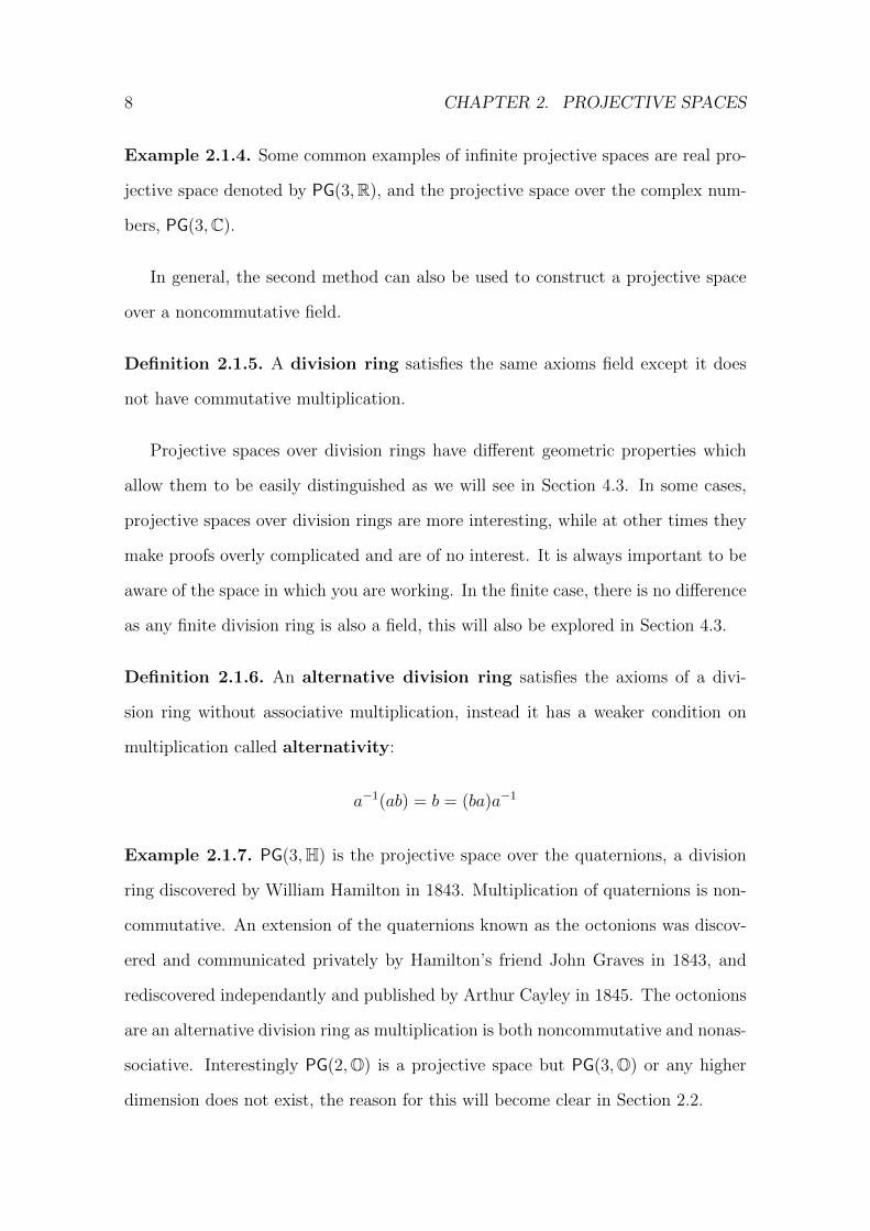
Example 2.1.7. PG(3,H) is the projective space over the quaternions, a division
ring discovered by William Hamilton in 1843. Multiplication of quaternions is non-
commutative. An extension of the quaternions known as the octonions was discov-
ered and communicated privately by Hamilton’s friend John Graves in 1843, and
rediscovered independantly and published by Arthur Cayley in 1845. The octonions
are an alternative division ring as multiplication is both noncommutative and nonas-
sociative. Interestingly PG(2,O) is a projective space but PG(3,O) or any higher
dimension does not exist, the reason for this will become clear in Section 2.2.

2.1. DEFINITION 9
We end this introduction to projective spaces with a few definitions. The first
two definitions are perhaps the most important of all.
Definition 2.1.8. A set of points are collinear if they are all incident to the same
line. A set of lines are concurrent if they are all incident to the same point.
(a) Collinear points (b) Concurrent lines
Definition 2.1.9. Two triangles are centrally perspective if lines through their
corresponding vertices are concurrent. Two triangles are axially perspective if
the intersections of their corresponding sides are collinear.
(a) Centrally perspective (b) Axially perspective
Definition 2.1.10 (Harmonic conjugate). Given three collinear points A, B, C and
a noncollinear point L, let a line through C meet LA at M and LB at N . Let K
be the intersection of AN and BM . Then the point D = LK ∩AB is known as the
harmonic conjugate of C with respect to AB. See Figure 2.3.

10 CHAPTER 2. PROJECTIVE SPACES
A
L
B C
M
N
K
D
Figure 2.3: Harmonic Conjugate
2.2 Pappus and Desargues
We now introduce two theorems fundamental in the characterisation of projective
spaces, the theorems of Pappus (Pappus of Alexandria, ca. 300 A.D.) and Desargues
(Girard Desargues (1591-1661)).
Theorem 2.2.1 (Desargues,1648). Let A,B,C and A′, B′, C ′ be two triangles in a
projective plane. Then lines AA′, BB′ and CC ′ are concurrent if and only if the
points D = AB ∩ A′B′, E = AC ∩ A′C ′ and F = BC ∩B′C ′ are collinear.
In other words two triangles are centrally perspective if and only if they are
axially perspective.
Example 2.2.2. Desargues’ Theorem holds in any projective space of dimension 3
and above. The reasoning for this is explained on page 142 of The Four Pillars of
Geometry by John Stillwell [22].
Remark. We will see in Section 4.4 that Desargues does not follow from the
incidence axioms of a two dimensional projective space. However, in three dimen-
sions the basic incidence properties of points, lines and planes, namely that the
intersection of two distinct planes is a line, do imply Desargues’ Theorem.

2.2. PAPPUS AND DESARGUES 11
P
A′
B′
C′
A
C
B
D
F
E
Figure 2.4: Desargues’ Theorem
Theorem 2.2.3 (Pappus). Let g, h be two lines that intersect at point P . If distinct
points A,B,C lie on g and distinct points A′, B′, C ′ lie on h with A,B,C,A′, B′, C ′ 6=
P then the points D = AB′∩A′B, E = AC ′∩A′C and F = BC ′∩B′C are collinear.
A
P
A′
B
C
B′
C′
DE
F
Figure 2.5: Pappus’ Theorem
12 CHAPTER 2. PROJECTIVE SPACES
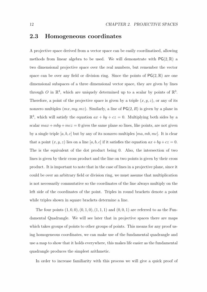
2.3 Homogeneous coordinates
A projective space derived from a vector space can be easily coordinatised, allowing
methods from linear algebra to be used. We will demonstrate with PG(2,R) a
two dimensional projective space over the real numbers, but remember the vector
space can be over any field or division ring. Since the points of PG(2,R) are one
dimensional subspaces of a three dimensional vector space, they are given by lines
through O in R3, which are uniquely determined up to a scalar by points of R3.
Therefore, a point of the projective space is given by a triple (x, y, z), or any of its
nonzero multiples (mx,my,mz). Similarly, a line of PG(2, R) is given by a plane in
R3, which will satisfy the equation ax + by + cz = 0. Multiplying both sides by a
scalar max+mby+mcz = 0 gives the same plane so lines, like points, are not given
by a single triple [a, b, c] but by any of its nonzero multiples [ma,mb,mc]. It is clear
that a point (x, y, z) lies on a line [a, b, c] if it satisfies the equation ax+ by+ cz = 0.
The is the equivalent of the dot product being 0. Also, the intersection of two
lines is given by their cross product and the line on two points is given by their cross
product. It is important to note that in the case of lines in a projective plane, since it
could be over an arbitrary field or division ring, we must assume that multiplication
is not necessarily commutative so the coordinates of the line always multiply on the
left side of the coordinates of the point. Triples in round brackets denote a point
while triples shown in square brackets determine a line.
The four points (1, 0, 0), (0, 1, 0), (1, 1, 1) and (0, 0, 1) are referred to as the Fun-
damental Quadrangle. We will see later that in projective spaces there are maps
which takes groups of points to other groups of points. This means for any proof us-
ing homogeneous coordinates, we can make use of the fundamental quadrangle and
use a map to show that it holds everywhere, this makes life easier as the fundamental
quadrangle produces the simplest arithmetic.
In order to increase familiarity with this process we will give a quick proof of
2.3. HOMOGENEOUS COORDINATES 13
Pappus’ Theorem using homogeneous coordinates.
Proof. We start by making use of the fundamental quadrangle. A = (1, 0, 0), B =
(0, 1, 0), A′ = (1, 1, 1) and B′ = (0, 0, 1). The line through AB = [AB|1, AB|2, AB|3]
goes through (1, 0, 0) and (0, 1, 0) therefore it satisfies:
AB|1(1) + AB|2(0) + AB|3(0) = 0
AB|1(0) +B|2(1) +B|3(0) = 0
⇒ AB|1 = 0 and AB|2 = 0.
So, the line AB = [0, 0, 1] or z = 0. We can then calculate the line A′B′ in the same
way and find that A′B′ = [1,−1, 0], or x = y. The intersection of these two lines
P = (p1, p2, p3) must satisfy:
p3 = 0 and p1 − p2 = 0
⇒ p = (p1, p1, 0).
However up to a scalar this is the same point as (1, 1, 0) so the intersection of AB
with A′B′ is (1, 1, 0). Now C ′ is any point on A′B′ not equal to P so we choose to
let C ′ = (t, t, 1), t 6= 0, 1. It is easy to verify this point does indeed lie on the line
x = y but is not the same point as P . Similarly, C is any point on AB not equal to
P . Suppose C = (1, s, 0), s 6= 0, 1. We can now calculate the lines A′B, AB′, A′C,
AC ′. B′C, BC ′ and the points D, E and F .
Firstly we can see from inspection the line AB′ is y = 0 and A′B is x = z.
Therefore their intersection D = (d1, d2, d3) can easily be calculated as (d1, 0, d1)
which is the same point as (1, 0, 1). Next, the line BC ′ = [BC ′1, BC′2, BC
′3] passes
through (0, 1, 0) and (t, t, 1).
BC ′1(0) +BC ′2(1) +BC ′3(0) = 0 (B on BC ′)
BC ′1(t) +BC ′2(t) +BC ′3(1) = 0 (C ′ on BC ′)
⇒ BC ′ = [1, 0,−t].
14 CHAPTER 2. PROJECTIVE SPACES
The line B′C = [B′C1, B′C2, B
′C3] passes through (0, 0, 1) and (1, s, 0).
B′C1(0) +B′C2(0) +B′C3(1) = 0 (B′ on B′C)
B′C1(1) +B′C2(s) +B′C3(0) = 0 ( on B′C)
⇒ B′C = [−s, 1, 0].
Now F = (f1, f2, f3) is the intersection of BC ′ with B′C. So
f1 − tf3 = 0
f1 = tf3
and
−sf1 + f2 = 0
f2 = sf1.
Setting f3 as 1 gives f = (t, st, 1). The line A′C = [A′C1, A′C2, A
′C3] passes through
(1, 1, 1) and (1, s, 0).
A′C1(1) + A′C2(s) + A′C3(0) = 0 (C on A′C)
A′C1 = −A′C2(s)
A′C1(1) + A′C2(1) + A′C3(1) = 0 (A′ on A′C)
−A′C2(s) + A′C2(1) + A′C3(1) = 0
A′C2(1− s) = −A′C3
⇒ A′C = [−s, 1, s− 1].
Lastly the line AC ′ = [AC ′1, AC′2, AC
′3] passes through (1, 0, 0 and (t, t, 1):
AC ′1(1) + AC ′2(0) + AC ′3(0) = 0 (A on AC ′)
AC ′1 = 0
AC ′1(t) + AC ′2(t) + AC ′3(1) = 0 (C ′ on AC ′)
⇒ AC ′ = [0, 1,−t].
2.3. HOMOGENEOUS COORDINATES 15
The intersection of these two lines, E = (e1, e2, e3) must satisfy:
e2 − te3 = 0
e2 = te3
and
−se1 + e2 + (s− 1)e3 = 0
se1 = (s+ t− 1)e3
Setting e3 = s gives E = (s + t − 1, ts, s). In order for these three points to be
collinear, then E must be a linear combination of F and D:
(s+ t− 1, ts, s) = (t, st, 1) + (s− 1)(1, 0, 1).(1)
This shows that E can be expressed as a linear combination of D and F , therefore
D, E and F are collinear.
Remark. Remember that multiplication is not always commutative so the above
proof only holds in the case where ts = st in (1).
Chapter 3
Projective Planes
3.1 Definition
From now on we narrow our focus to the study of projective spaces of geomet-
ric dimension 2 only. Since they contain only points and lines, we will call them
projective planes.
Since a projective plane is a projective space, it satisfies the projective space
axioms. However, it turns out that Axiom 2, the Veblen-Young Axiom, can be
replaced by a stronger statement which says that every pair of lines meet in exactly
one point.
P1. For every pair of distinct points there exists a unique line that is incident
to both.
P2. Every pair of lines meet in exactly one point.
P3. Every line is incident to at least three points.
P4. There are at least two lines.
Once again a projective plane can be finite or infinite. In both cases, it can be
shown as a consequence of the axioms that there are the same number of points and
lines, and every line is incident to the same number of points. The bijection between
the points on a line a and another line b will become clear in Section 3.4.
16

3.1. DEFINITION 17
Definition 3.1.1. The order of a projective plane is defined as the integer n such
that each line is incident to n + 1 points, each point is incident to n + 1 lines, and
there are n2 + n+ 1 points and n2 + n+ 1 lines.
Example 3.1.2. The Fano plane, named after Gino Fano, shown in Figure 3.1, is
the smallest example of a finite projective plane. It has order n = 2 meaning there
are seven points and seven lines. There are three lines through each point and three
points on each line.
Figure 3.1: Fano Plane
It turns out that all known examples of finite projective planes have prime power
order. As an aside, whether or not there exist finite projective planes of nonprime
power order is still an open question in finite geometry. The smallest order for
which no projective plane has yet been found but existence has not yet been proven
impossible is 12. The only other known condition on the order of a finite projective
plane is given by the following theorem attributed to Richard Bruck and Herbert
Ryser. Interestingly the theorem dates back to 1949 however no further progress
has yet been made despite it being an active area of study ??.
Theorem 3.1.3 (Bruck-Ryser, 1946). If n ≡ 1 or 2 mod 4 and there exists a
projective plane of order n, then n must be expressible as the sum of two squares.
18 CHAPTER 3. PROJECTIVE PLANES
Example 3.1.4. There is no projective plane of order 14 because 14 ≡ 2 (mod 4)
but it is easy to check that there are no two square numbers that sum to 14.
In addition to the four axioms for a projective plane, call them P1 - P4, we will
also give an optional axiom which will turn out to play an important role in the
classification of projective planes.
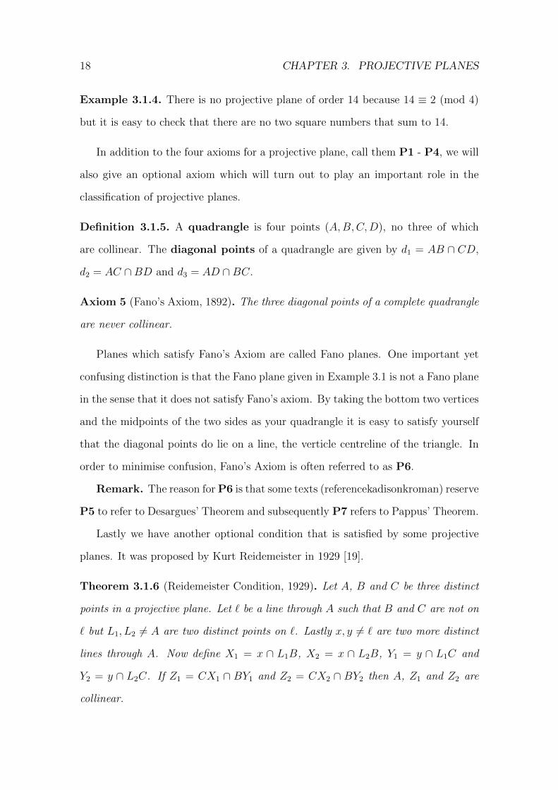
Definition 3.1.5. A quadrangle is four points (A,B,C,D), no three of which
are collinear. The diagonal points of a quadrangle are given by d1 = AB ∩ CD,
d2 = AC ∩BD and d3 = AD ∩BC.
Axiom 5 (Fano’s Axiom, 1892). The three diagonal points of a complete quadrangle
are never collinear.
Planes which satisfy Fano’s Axiom are called Fano planes. One important yet
confusing distinction is that the Fano plane given in Example 3.1 is not a Fano plane
in the sense that it does not satisfy Fano’s axiom. By taking the bottom two vertices
and the midpoints of the two sides as your quadrangle it is easy to satisfy yourself
that the diagonal points do lie on a line, the verticle centreline of the triangle. In
order to minimise confusion, Fano’s Axiom is often referred to as P6.
Remark. The reason for P6 is that some texts (referencekadisonkroman) reserve
P5 to refer to Desargues’ Theorem and subsequently P7 refers to Pappus’ Theorem.
Lastly we have another optional condition that is satisfied by some projective
planes. It was proposed by Kurt Reidemeister in 1929 [19].
Theorem 3.1.6 (Reidemeister Condition, 1929). Let A, B and C be three distinct
points in a projective plane. Let ` be a line through A such that B and C are not on
` but L1, L2 6= A are two distinct points on `. Lastly x, y 6= ` are two more distinct
lines through A. Now define X1 = x ∩ L1B, X2 = x ∩ L2B, Y1 = y ∩ L1C and
Y2 = y ∩ L2C. If Z1 = CX1 ∩ BY1 and Z2 = CX2 ∩ BY2 then A, Z1 and Z2 are
collinear.

3.2. DUALITY 19
AB
C
L2
L1
X1
X2
Y1
Y2
Z1
Z2
Figure 3.2: Reidemeister Condition
3.2 Duality
One extraordinary property of projective planes is the correspondence between
points and lines. Let π be aprojective plane, then taking any theorem which holds in
π and interchanging the words ‘points’ and ‘lines’, as well as making the necessary
grammatical changes produces a dual theorem. Note that the dual theorem will
not necessarily hold in π. We practice this idea by recalling P1, that every pair of
points lies on a unique line. The dual of this statement is that every pair of lines
intersect in a unique point which is precisely P2. Also, two triangles are centrally
perspective if lines through their corresponding vertices are concurrent. The dual of
this statement is two triangles are in perspective if the intersection points of their
corresponding sides are collinear, which is the definition of axially perspective. The
dual of a dual statement is the original statement.
Definition 3.2.1. A theorem is called self dual if swapping the terms ‘points’ and
‘lines’ produces the same theorem.

20 CHAPTER 3. PROJECTIVE PLANES
Example 3.2.2. Desargues’ Theorem says that two triangles are centrally perspec-
tive if and only if they are axially perspective. Dualising this theorem we get that
two triangles are axially perspective if and only if they are centrally perspective
which is exactly the same statement. Therefore Desargues’ Theorem is self dual.
Theorem 3.2.3 (Principle of Duality, Chapter 2.4 [21]). If a theorem is deducible
from the axioms, then its dual is also deducible from the axioms.
Simply writing down the dual of each statement used to prove the original the-
orem will result in a proof of the dual theorem.
Given a projective plane π, consider a bijective map ϕ which takes the points to
lines and lines to points that preserves incidences. For example let P be a point on
` then ϕ(`) will be a point on the line ϕ(P ). This map will create another structure
satisfying the axioms of a projective plane. We will call it the dual plane, π∗. The
dual of any theorem which holds in π will be a theorem in π∗. Also, applying ϕ
twice produces the same mapping as the identity.
Example 3.2.4. Recall that the coordinates of points are given in round brackets
and lines are denoted by square brackets. The map taking (a1, a2, a3) to [a1, a2, a3]
is called the standard duality.
A plane is called self dual if π and π∗ are isomorphic. Another way to interpret
the Principle of Duality is that the dual of a theorem will hold in π as well as in π∗
if and only if it is self dual.
Example 3.2.5. All projective planes PG(2, D) where D is a division ring are self
dual. The reason for this will become clear with Theorem 4.3.1

3.3. COLLINEATIONS 21
3.3 Collineations
Definition 3.3.1. A collineation is a bijection from a projective plane to itself
that preserves lines.
In other words a collineation is a map acting on the points of a projective plane
that is an automorphism. For example if we have a collineation ϕ and points
P1, P2, . . . , Pn are collinear then the image of each of the points under ϕ will still be
collinear.
Another important property of projective planes is that the set of all collineations
of a projective plane together with an operation which is just the standard compo-
sition of maps, forms a group which we denote by Aut(π). Usually, a collineation
group refers to a subgroup of Aut(π). Studying the collineation groups of projective
planes is another way to classify them.
Definition 3.3.2. Given a group G and a set Ω, a group action α is a function
α : G× Ω→ Ω such that:
1) ωe = ω where e is the identity of G,
2) ((ω)g)h = ω(g·h), for all g, h ∈ G.
Example 3.3.3. Let PG(2, F ) be the projective plane made from a vector space
over F and M be an element of the general linear group, which is the group of 2× 2
matrices with entries from F , denoted GL(2, F ). M will induce a collineation on
PG(2, F ) and the group action of GL(2, F ) forms a collineation group denoted by
PGL(2, F ).
A point is fixed by a collineation if ϕ(P ) = P . Similarly a line is fixed if
ϕ(`) = ` where ` simply refers to the set of points on that line, in any order. In
other words the line is fixed set-wise but the points may be permuted around.
Definition 3.3.4. A line fixed point-wise by a collineation is called an axis. Here
point-wise means that the line is fixed and the points remain in the same order. It

22 CHAPTER 3. PROJECTIVE PLANES
is a stronger condition than the line just being fixed. A point through which all the
lines are fixed by a collineation is called a centre.
A collineation is a central collineation if it has a centre.
Theorem 3.3.5 (Piper and Hughes, Theorem 4.9 [9]). A collineation has a centre
if and only if it has an axis, and a collineation with more than one centre or axis is
the identity.
Definition 3.3.6. A central collineation is an elation if the centre lies on the axis
and a homology if the centre does not lie on the axis.
Example 3.3.7. Recall that a point is incident with a line if Ax + By + Cz = 0
where (x, y, z) are the homogeneous coordinates of the point and [a, b, c] are the
coordinates of the line. Consider the following collineation
(x, y, z) 7→ (X + cz, y, z)
[a, b, c] 7→ [a, b, c− ac]
If a line is incident with (1, 0, 0) it must satisfy a(1) + b(0) + b(0) = 0 therefore it
has a = 0 and has the general form [0, b, c]. By the collineation this line is mapped
to [0, b, c − (0)c] = [0, b, c] so clearly it is fixed, therefore (1, 0, 0) is the centre. Use
the same technique to show every point on the line [0, 0, 1] must be of the form
(x, y, 0) which will be mapped to (x+ c(0), y, 0) = (x, y, 0) and again it is clear that
each of these points is fixed so the line [0, 0, 1] is the axis.
Also (1, 0, 0) is a point of the form (x, y, 0) and so it too lies on the axis, meaning
this specific central collineation is an elation.
Definition 3.3.8. Let V be a point and ` a line in a projective plane. The plane is
(V, `)-transitive if for any distinct points A and B not on ` with A 6= B 6= V there
is a central collineation with centre V and axis ` that maps A to B.

3.4. PERSPECTIVITIES AND PROJECTIVITIES 23
O
A′B′
C′
A
B
C
`
`′
Figure 3.3: Perspectivity with centre O
3.4 Perspectivities and Projectivities
Given a line ` and a point O not on `, a perspectivity from ` to `′ is a correspon-
dence of the points on ` with the points on `′ defined in the following way: if A ∈ `
then A′ ∈ `′ where A′ = AO ∩ `′, Z = ` ∩ `′ gets mapped to itself. The point O is
the centre of the perspectivity.
It is a clear consequence of P1, that for any two points there is a unique line
that is incident to both, that a perspectivity will form a bijection between the points
of ` and `′. This is why we can be sure there are the same number of points on each
line. If points P1, P2, . . . , Pn are sent to P ′1, P′2, . . . , P
′n by a perspectivity with centre
O and then to P ′′1 , P′′2 , . . . , P
′′n by another perspectivity with centre O′, there may
not exist a point which is the centre of a perspectivity directly from P1, P2, . . . , Pn
to P ′′1 , P′′2 , . . . , P
′′n . Instead, if we wish to transform points P1, P2, . . . , Pn directly to
P ′′1 , P′′2 , . . . , P
′′n we can use a projectivity.
Definition 3.4.1. A projectivity is a bijective map from the points on a line ` to
the points on a line `′ which can be expressed as the product of a finite number of

24 CHAPTER 3. PROJECTIVE PLANES
perspectivities.
It is clear that there exists a projectivity from any two points to any other two
points because the intersection of two lines is always a unique point, which can be
used as the centre of a perspectivity, but what about any three points? It turns out
that this is not always possible. Any three noncollinear points can be projected to
any other three noncollinear points and any three collinear points can be projected
to any three collinear points.
Theorem 3.4.2 (Fundamental Theorem of Projective Geometry, Kadison and Kro-
mann, Theorem 11.11,[10]). Given three distinct collinear points A, B and C, there
is exactly one projectivity which takes them to another three distinct collinear points
A′, B′ and C ′.
3.5 Planar Ternary Rings
We have already seen one method for coordinatising a projective plane over a vector
space, those of the form PG(2, D), where D is a field or division ring. However, not
all projective planes are defined in this way. We need another way to coordinatise
these other planes, in order to establish whether two given projective planes are
isomorphic. It turns out these other planes can be coordinatised using planar ternary
rings.
Definition 3.5.1. A Planar Ternary Ring or just ternary ring is any set R which
includes the elements 0 and 1 together with a ternary operation T which takes any
three ordered elements a, b, c of R and prescribes a unique element T (a, b, c) of R
such that the following properties hold:
T1. T (0, b, c) = T (a, 0, c) = c, for all a, b, c ∈ R.
T2. T (a, 1, 0) = T (1, a, 0) = a, for all a ∈ R.
3.5. PLANAR TERNARY RINGS 25
T3. If a, b, c, d ∈ R with a 6= c then the equation T (x, a, b) = T (x, c, d) has a
unique solution for x.
T4. If a, b, c ∈ R then there is a unique x ∈ R such that T (a, b, x) = c.
T5. If a, b, c, d ∈ R with a 6= c then the system of equations
T (a, x, y) = b,
T (c, x, y) = d,
has a unique solution for (x, y).
Example 3.5.2. A division ring (R,+,×) together with the ternary operation
T (a, b, c) = ab+ c satisfies the five conditions and therefore forms a ternary ring.
The ternary ring is denoted by (R, T ). Any projective plane of order n can be
coordinatised by a planar ternary ring with n elements. A step by step explanation
of how this can be done and why it works for a projective planes, not just those
defined over a vector space, may be found in Projective Planes by Piper and Hughes
[9], or Projective Geometry and Modern Algebra by Kadison and Kromann [10].
We will now introduce the concept of projective addition and multiplication.
Given a ternary operation which takes three elements to one element, define a binary
operation called addition which takes two elements to one element by the following
rule
a+ b = T (a, 1, b).
To interpret this geometrically let A = (a, a) and B = (b, b) be two points. Take
the line through A and B and call it the x-axis and take another line and call it
the y-axis. Now consider a third line `, for simplicity we will say this line is parallel
to the x-axis but recall this just means that their intersection lies on the line at
infinity. Then A+B is given by the following construction:
1. Take a line m from A to the intersection of ` and the y-axis.
2. Take a line n from B parallel to the y-axis.

26 CHAPTER 3. PROJECTIVE PLANES
A B A+B
`
m
nk
O
Figure 3.4: Projective addition
3. Take a line k through the intersection of n and ` which is parallel to m
Now A+B is the intersection of k with the x-axis.
Multiplication is also a binary operation defined by
a · b = T (a, b, 0).
Again to interpret this geometrically let A = (a, a) and B = (b, b). Take the line
through A and B and call it the x-axis and another line called y-axis and let their
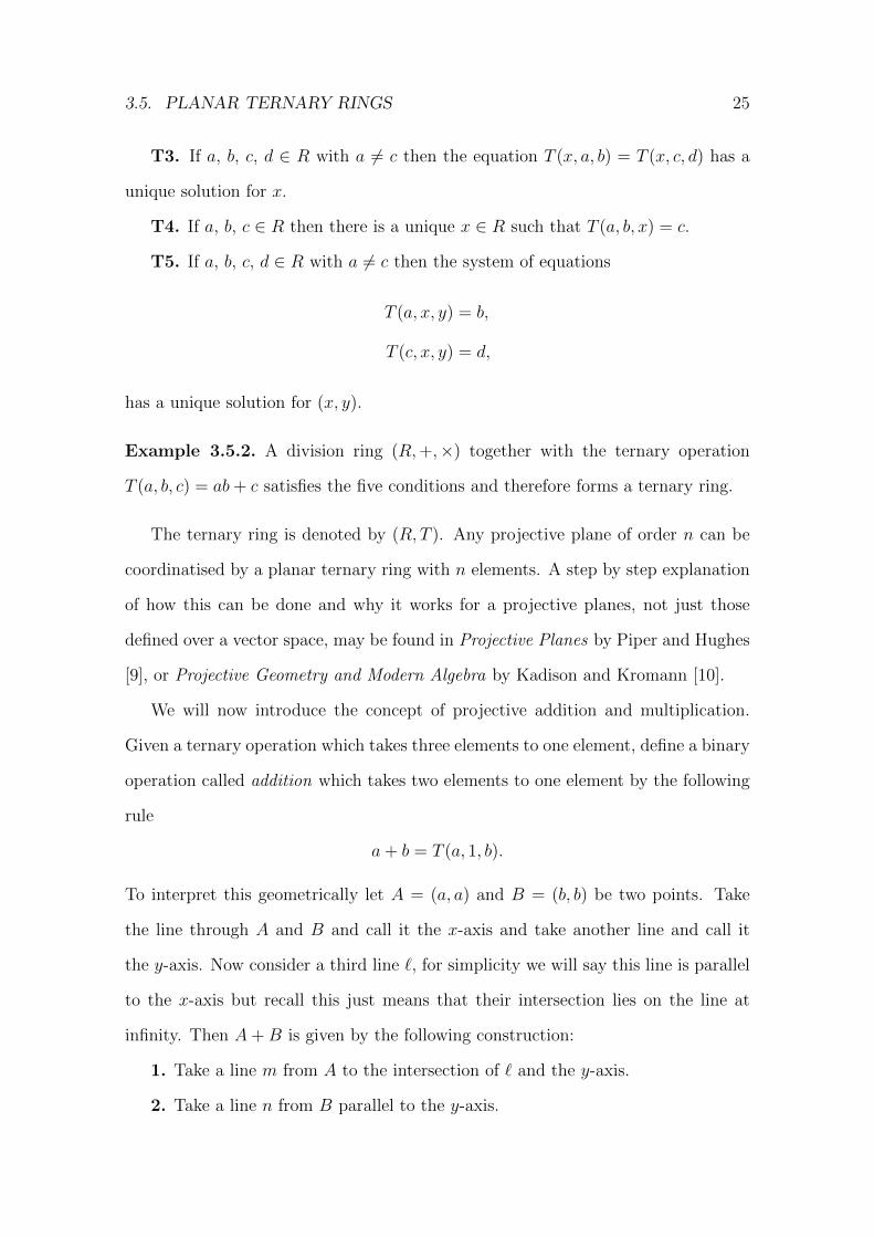
intersection be O. Choose a point on the x-axis other than O to denote by 1x, and
choose a different point on the y-axis other than O to denote by 1y.
1. Take a line m from 1x to 1y.
2. Take a line n from A to 1y.
3. Take a line k from through of B which is parallel to m.
4. Take a line j through the intersection of k and the y-axis which is parallel to n.
Now A ·B is the intersection of j with the x-axis.
Definition 3.5.3. A loop is a nonempty set G together with a binary operation ·
such that:
(a) If a, b ∈ G then a · x = b has a unique solution for x.
(b) If a, b ∈ G then y · a = b has a unique solution for y.
(c) G has an element e such that e · x = x · e = x for all x ∈ G. The element e
is referred to as the identity.
3.5. PLANAR TERNARY RINGS 27
O 1x A B
1y
A ·B
m
nk
j
Figure 3.5: Projective multiplication
Example 3.5.4. If (R, T ) is a planar ternary ring then (R,+) forms a loop with 0
as its identity and (R\0, ·) forms a loop with 1 as its identity. Note also that a
group is a loop such that every element a has an inverse a−1 with aa−1 = a−1a = e.
Definition 3.5.5. A ternary ring R, T is called a Veblen-Wedderburn system
if:
VW1. (R,+) forms an abelian group,
VW2. (R\0, ·) forms a loop with 1 as the identity,
VW3. a · 0 = 0 · a = 0 for all a ∈ R,
VW4. R has right distributivity. i.e. (a+ b) · c = a · c+ b · c for all a, b, c ∈ R.
Example 3.5.6. The octonions are a finite alternative division ring. Multiplication
of the octonions is defined using a Cayley table as it is both nonassociative and
noncommutative. However, on inspection of the Cayley table, it is possible to see
that the octonions form a Veblen-Wedderburn system.

Chapter 4
Pappus and Desargues in
Projective Planes
4.1 Theorem Hierarchy
In a projective plane, the theorems of Pappus and Desargues are simply propositions
which may or may not be true in a given plane. (However they are still referred
to as theorems as they were originally studied in real projective space where they
are always true). A projective plane in which Desargues’ Theorem holds is called
Desarguesian. A projective plane in which Pappus’ Theorem holds is called Pap-
pian.
As well as Pappus and Desargues there are also a number of other theorems
which follow as direct results. For this reason it would make sense for them to be
corollaries, however they are still referred to as theorems in their own right because
there are non-Desarguesian planes in which these theorems do hold. This will be
covered in more detail in Sections 4.3 and 4.4. The first important thing to note is
that Desargues’ Theorem is self dual. We have already seen why in Example 3.2.2.
Next we consider a special case of Desargues’ Theorem known as Little Desar-
gues’ Theorem, where the centre of perspectivity lies on the axis of perspectivity.
28

4.1. THEOREM HIERARCHY 29
P
AC
B
B′
C′
F
E
A′
D
Figure 4.1: Little Desargues
Theorem 4.1.1 (Little Desargues). If triangles A,B,C and A′, B′, C ′ are in per-
spective from a point P and the points D = AB ∩ A′B′ and E = AC ∩ A′C ′ are
collinear with P , then the point F = BC ∩B′C ′ is also collinear with P , D and E.
Another special case arises when one vertex of one triangle lies on the corre-
sponding side of the other.
Theorem 4.1.2 (Special Desargues). If triangles A,B,C and A′, B′, C ′ are in per-
spective from a point P such that B′ lies on AC then D = AB∩A′B′, E = AC∩A′C ′
and F = BC ∩B′C ′ are collinear.
Desargues’ Theorem is referred to as D11 because it contains 11 free parame-
ters and Little and Special Desargues’ are both referred to as D10 because they
both involve one extra incidence and therefore have one less free parameter. The
nomenclature can be attributed first to Ruth Moufang [14], but was also adopted
by Heyting. A projective plane in which D10 holds is called a Moufang plane.

30 CHAPTER 4. PAPPUS AND DESARGUES IN PROJECTIVE PLANES
P
A
C
B
B′
A′
C′
E
D
F
Figure 4.2: Special Desargues
Since the two theorems are referred to by the same term it is important to
establish that they are equivalent.
Theorem 4.1.3 (Heyting, Theorem 2.2.8,2.2.10 [6]). Little Desargues and Special
Desargues are equivalent.
Proof. (⇒) Let triangles A,B,C and A′, B′, C ′ be in perspective from a point P
such that B′ lies on AC. We want to show D = AB ∩ A′B′, E = AC ∩ A′C ′ and
F = BC ∩ B′C ′ are collinear. Note triangles DBF and A′PC ′ are in perspective
from B′ because D lies on A′B′ by the definition of D, B lies on PB′ because the
original two triangles are in perspective and F lies on B′C ′ by the definition of F ,
see Figure 4.2. Also A is the intersection of DB with A′P and C is the intersection
of FB with C ′P and B′ was defined to lie on AC so A, B′ and C are collinear.
Therefore we have two intersections of corresponding sides being collinear with the
centre of perspectivitity so by Little Desargues we know that the intersection of the
third pair of corresponding sides is also collinear, call it G = DF ∩ A′C ′. Now we
have that G lies on AC by Little Desargues and G also lies on A′C ′ by definition so
G must be the point of intersection of these two lines, but the intersection is unique

4.1. THEOREM HIERARCHY 31
and was already defined to be E, so G = E. We also have that G was on DF by
definition therefore E lies on DF , so D, E and F are collinear.
(⇐) Let triangles A,B,C and A′, B′, C ′ be in perspective from a point P such
that the points D = AB ∩ A′B′ and E = AC ∩ A′C ′ are collinear with P , we want
to show F = BC ∩B′C ′ is also collinear with P , D and E. Note triangles BPC and
DA′E are in perspective from A because D lies on AB by definition, A′ lies on PA
because the two original triangles are in perspective and E lies on AC by definition.
Also we have that P lies on ED by construction, see Figure 4.1. Therefore we have
two triangles in perspective from a point, one of which has a vertex lying on a side of
the other, so by Special Desargues we know the intersections of their corresponding
sides are collinear. The intersection of BP with A′D is B′, PC ∩ A′E is C ′ and
let BC ∩ ED = G, so B′C ′G are collinear. However G lies on BC and B′C ′ but
we already defined their unique intersection to be F so G = F . We also know that
G lies on ED by definition which means that F lies of ED so P , D, E and F are
collinear.
We now look at adding another incidence to Desargues’ Theorem, two extra in
total, this will give us D9. In the same way as D10, Heyting uses D9 to refer to
a group of theorems, five in total, representing the five different ways to configure
Desargues’ Theorem with two extra incidences. In fact, there are more than five
ways to add two incidences but the others all become trivial. We will focus only on
what Heyting calls D9 and DI9. Only these two are known to be equivalent so we will
refer to them both as D9, proofs can be found in Heyting’s book, Theorems 2.2.17
and 2.2.18 [6]. The other three are known to follow from D9 but are not known to
imply it, these are still open questions.
Theorem 4.1.4 (D9). Let triangles A,B,C and A′, B′, C ′ be in perspective from a
point P . If:

32 CHAPTER 4. PAPPUS AND DESARGUES IN PROJECTIVE PLANES
a) the point B′ lies on AC and B lies on A′C ′,
or
b) the point A′ lies on BC and B′ lies on AC,
then D = AB ∩ A′B′, E = AC ∩ A′C ′ and F = BC ∩B′C ′ are collinear.
Theorem 4.1.5 (Moufang [14]). Desargues’ Theorem implies D10, which implies D9.
We don’t give a formal proof because it is fairly obvious, it follows as an immedi-
ate consequence of the fact that D9 is just one specific configuration of D10 and D10
is one specific configuration of Desargues. On the other hand, are there any planes
in which the reverse of this theorem hold? Is it possible that any of the degenerate
versions of Desargues’ Theorem imply stronger ones?
Theorem 4.1.6 (Heyting, Theorem 2.4.6 [6]). In a projective plane satisfying P6,
D9 implies D10.
Remark. It is not known whether D9 implies D10 in general, this is still an open
problem. However, Heyting is able to prove the following Harmonic Proposition: If
D is the harmonic conjugate of C with respect to AB and D is never equal to C,
then D10 is equivalent to D9. We wish to refer the reader to the proof of Theorem
2.4.6 in Heyting. Therefore it suffices for us to show that this condition on the
harmonic conjugate is equivalent to P6.
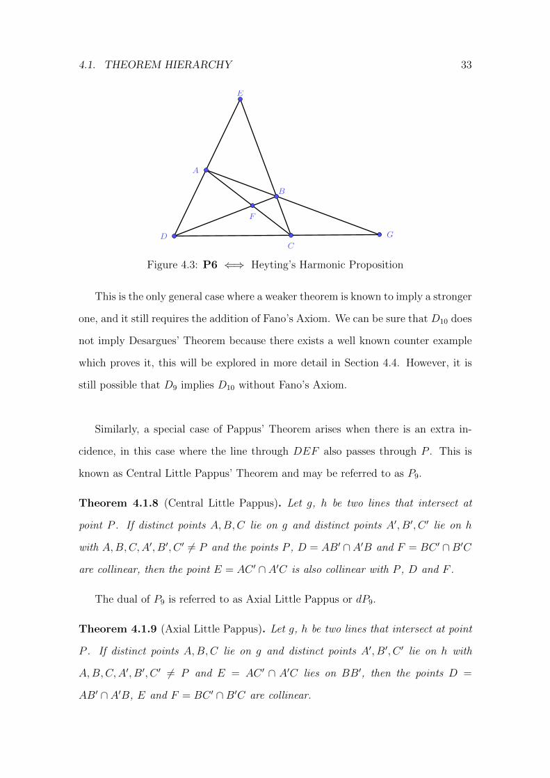
Proposition 4.1.7. P6 is equivalent to the harmonic conjugate of a point never
being equal to itself.
Proof. Let A, B, C, and D be four points, no three of which are collinear. P6 says
that E = AD ∩ BC, F = AC ∩ BD and G = AB ∩ CD are never collinear. This
means that EF ∩CD, which is precisely the harmonic conjugate of G with respect
to CD is never G. Conversely let the harmonic conjugate of G with respect to CD
be a point H not equal to G. Then H = EF ∩ CD. Since two lines intersect in a
unique point then EF cannot pass through G as G also lies on CD.
4.1. THEOREM HIERARCHY 33
E
DC
G
A
B
F
Figure 4.3: P6 ⇐⇒ Heyting’s Harmonic Proposition
This is the only general case where a weaker theorem is known to imply a stronger
one, and it still requires the addition of Fano’s Axiom. We can be sure that D10 does
not imply Desargues’ Theorem because there exists a well known counter example
which proves it, this will be explored in more detail in Section 4.4. However, it is
still possible that D9 implies D10 without Fano’s Axiom.
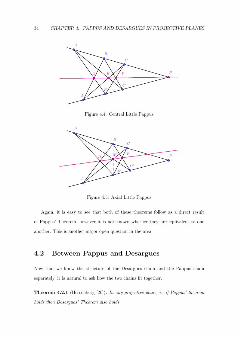
Similarly, a special case of Pappus’ Theorem arises when there is an extra in-
cidence, in this case where the line through DEF also passes through P . This is
known as Central Little Pappus’ Theorem and may be referred to as P9.
Theorem 4.1.8 (Central Little Pappus). Let g, h be two lines that intersect at
point P . If distinct points A,B,C lie on g and distinct points A′, B′, C ′ lie on h
with A,B,C,A′, B′, C ′ 6= P and the points P , D = AB′ ∩A′B and F = BC ′ ∩B′C
are collinear, then the point E = AC ′ ∩ A′C is also collinear with P , D and F .
The dual of P9 is referred to as Axial Little Pappus or dP9.
Theorem 4.1.9 (Axial Little Pappus). Let g, h be two lines that intersect at point
P . If distinct points A,B,C lie on g and distinct points A′, B′, C ′ lie on h with
A,B,C,A′, B′, C ′ 6= P and E = AC ′ ∩ A′C lies on BB′, then the points D =
AB′ ∩ A′B, E and F = BC ′ ∩B′C are collinear.
34 CHAPTER 4. PAPPUS AND DESARGUES IN PROJECTIVE PLANES
P
A
B
A′
B′
D E
C
C′
F
Figure 4.4: Central Little Pappus
P
A
A′
C
C′
E
B
B′
DF
Figure 4.5: Axial Little Pappus
Again, it is easy to see that both of these theorems follow as a direct result
of Pappus’ Theorem, however it is not known whether they are equivalent to one
another. This is another major open question in the area.
4.2 Between Pappus and Desargues
Now that we know the structure of the Desargues chain and the Pappus chain
separately, it is natural to ask how the two chains fit together.
Theorem 4.2.1 (Hessenberg [20]). In any projective plane, π, if Pappus’ theorem
holds then Desargues’ Theorem also holds.
4.2. BETWEEN PAPPUS AND DESARGUES 35
Remark. The proof is not given here but it is geometric in nature. It was origi-
nally attributed to Gerhard Hessenberg who published the result in 1905. Although
he was correct his original proof didn’t cover all possible configurations and was
incomplete. The first complete proof was given by Arno Cronheim in 1953.
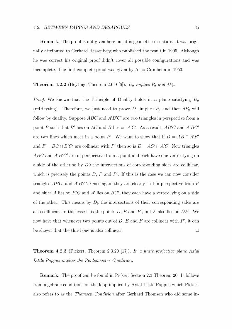
Theorem 4.2.2 (Heyting, Theorem 2.6.9 [6]). D9 implies P9 and dP9.
Proof. We known that the Principle of Duality holds in a plane satisfying D9
(refHeyting). Therefore, we just need to prove D9 implies P9 and then dP9 will
follow by duality. Suppose ABC and A′B′C ′ are two triangles in perspective from a
point P such that B′ lies on AC and B lies on A′C ′. As a result, AB′C and A′BC ′
are two lines which meet in a point P ′. We want to show that if D = AB ∩ A′B′
and F = BC ∩B′C ′ are collinear with P ′ then so is E = AC ′ ∩A′C. Now triangles
ABC and A′B′C ′ are in perspective from a point and each have one vertex lying on
a side of the other so by D9 the intersections of corresponding sides are collinear,
which is precisely the points D, F and P ′. If this is the case we can now consider
triangles ABC ′ and A′B′C. Once again they are clearly still in perspective from P
and since A lies on B′C and A′ lies on BC ′, they each have a vertex lying on a side
of the other. This means by D9 the intersections of their corresponding sides are
also collinear. In this case it is the points D, E and P ′, but F also lies on DP ′. We
now have that whenever two points out of D, E and F are collinear with P ′, it can
be shown that the third one is also collinear.
Theorem 4.2.3 (Pickert, Theorem 2.3.20 [17]). In a finite projective plane Axial
Little Pappus implies the Reidemeister Condition.
Remark. The proof can be found in Pickert Section 2.3 Theorem 20. It follows
from algebraic conditions on the loop implied by Axial Little Pappus which Pickert
also refers to as the Thomsen Condition after Gerhard Thomsen who did some in-
36 CHAPTER 4. PAPPUS AND DESARGUES IN PROJECTIVE PLANES
P
A′
B′
C′B
C
A
P ′
D
EF
Figure 4.6: D9 implies Axial Little Pappus
fluential work on the subject in the early 1930s. More on the algebraic consequences
of each of these geometric propositions will be covered in Section 4.3.
Theorem 4.2.4 (Kallaher 1967 [11]). In a projective plane where the coordinatising
ternary ring is a Veblen-Wedderburn system with the condition
(xy)(zx) = (x(yz))x, for all x, y, z ∈ R,(2)
Axial Little Pappus implies D10.
Remark. This result was published in a paper by Michael Kallaher in 1967.
His main result was to show that a Reidemeister plane is a Moufang plane if it
is coordinatized by a Veblen-Wedderburn system satisfying (2). This result then
follows as a corollary thanks to Theorem 4.2.3.
Since D9 is implied by all the other versions of Desargues’ Theorem, that puts
P9 and dP9 at the very bottom of the picture as the weakest two theorems while
Pappus implies everything so it sits right at the top as the strongest. This vertical
hierarchy will be reinforced in the following section as it is mirrors the algebraic
properties of the structures coordinatising the planes.

4.2. BETWEEN PAPPUS AND DESARGUES 37
Known relationships between geometric propositions are summarised in Figure
4.7. Each arrow in the diagram can be attributed to one of Hessenberg, Pickert and
Heyting, where an arrow means ‘implies’, no arrow means ‘does not imply’ and a
dotted arrow suggests it is still an open problem.
Pappus
Desargues
P9
dP9
D10
D9
D9 + P6
+VW*
Figure 4.7: Known Relationships between Geometric Propositions

38 CHAPTER 4. PAPPUS AND DESARGUES IN PROJECTIVE PLANES
4.3 Algebraic Consequences
It turns out that the veracity of these geometric propositions in a projective plane
reveals important information about the algebraic structure of the planar ternary
rings that coordinatise it, and so they can be used to characterise projective planes.
Since we know the geometric theorem hierarchy we can also construct a correspond-
ing algebraic structure hierarchy. The first major result is traditionally attributed
to Hilbert.
Theorem 4.3.1 (Hilbert [7]). A projective plane is isomorphic to PG(2, D), D a
division ring, if and only if it satisfies Desargues’ theorem.
Proof. (⇐) A plane isomorphic to PG(2, D) can be coordinatised using homogeneous
coordinates. Therefore we can prove Desargues’ Theorem algebraically, like we did
with Pappus’ Theorem earlier. Again we start by making use of the Fundamental
Quadrangle. Let B = (1, 0, 0), C = (0, 1, 0), B′ = (1, 1, 1) and C ′ = (0, 0, 1). Now
P = BB′ ∩ CC ′. We can see by inspection that BB′ is the line y = z and CC ′ is
the line x = 0. Therefore, their intersection is of the form (0, s, s) for some s ∈ D,
which is the same point as (0, 1, 1). A is a point not on BB′ or CC ′, so we are free
to choose A = (1, 0, 1). Now the line PA has:
PA1(0) = PA2(1) + PA3(1) = 0 (P on AP )
PA1(1) = PA2(0) + PA3(1) = 0 (A on AP )
⇒ PA1 = PA2 = −PA3
So the line PA = [1, 1,−1]. This is also the line x + y = z. Triangles ABC and
A′B′C ′ will be in perspective from P if A′ is any point on PA so let A′ = (1,m, 1+m).
Now we are ready to calculate D = AB∩A′B′, E = AC∩A′C ′ and F = BC∩B′C ′.
Firstly by inspection we see that BC is the line z = 0 and B′C ′ is the line y = x so
D = (1, 1, 0). Next, we can easily see that AC is the line x = z while the line A′C ′

4.3. ALGEBRAIC CONSEQUENCES 39
has:
A′C ′1(0) + A′C ′2(0) + A′C ′3(1) = 0 (C ′ on A′C ′)
A′C ′1(1) + A′C ′2(m) + A′C ′3(1 +m) = 0 (A′ on A′C ′)
A′C ′1 = −A′C ′2(m)
So A′C ′ = [m,−1, 0] or mx = y. The intersection of x = z and mx = y is the point
(1,m, 1), so E = (1,m, 1). Lastly AB is the line y = 0 and A′B′ has:
A′B′1(1) + A′B′2(1) + A′B′3(1) = 0 (B′ on A′B′)(1)
A′B′1(1) + A′B′2(m) + A′B′3(1 +m) = 0(A′ on A′B′)(2)
A′B′2(m− 1) + A′B′3(m) = 0 ((2) subtract (1))
A′B′2(m− 1) = −A′B′3(m)
and
A′B′1 = −A′B′2 − A′B′3
From this we get that A′B′ = [−1,m, 1 −m]. The intersection of AB with A′B′ is
therefore (1−m, 0, 1) so F = (1−m, 0, 1). In order for D, E and F to be collinear,
we must be able to express E as a linear combination of the coordinates for D and
F . Note that
(1,m, 1) = m(1, 1, 0) + (1−m, 0, 1).
This implies that D, E and F are collinear.
(⇒) Recall the description of projective addition and multiplication defined in Sec-
tion 3.5. Once the concepts of projective addition and multiplications are defined we
can prove, for example, that multiplication is associative using Desargues’ Theorem.
Regard Figure 4.10. Lines of the same colour are parallel, remembering that
this just means they intersect at a point on `∞. Consider the triangle with the
vertices P , (AB) and (AB)1y ∩ BP and the triangle with vertices Q, A(BC) and
Q(BC)∩R(A(BC)). Each of these triangles has a pink side, a blue side and a black
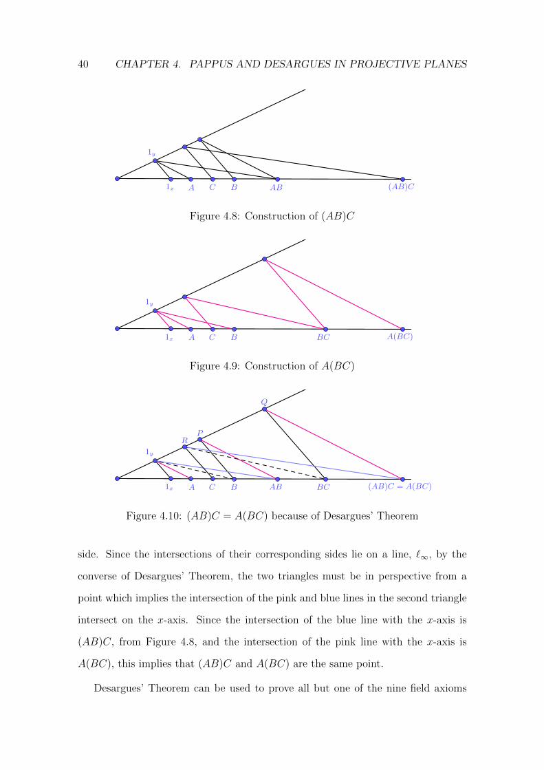
40 CHAPTER 4. PAPPUS AND DESARGUES IN PROJECTIVE PLANES
1x
1y
A B ABC (AB)C
Figure 4.8: Construction of (AB)C
1x
1y
A BC A(BC)BC
Figure 4.9: Construction of A(BC)
1x
1y
A B
P
ABC
Q
(AB)C = A(BC)BC
R
Figure 4.10: (AB)C = A(BC) because of Desargues’ Theorem
side. Since the intersections of their corresponding sides lie on a line, `∞, by the
converse of Desargues’ Theorem, the two triangles must be in perspective from a
point which implies the intersection of the pink and blue lines in the second triangle
intersect on the x-axis. Since the intersection of the blue line with the x-axis is
(AB)C, from Figure 4.8, and the intersection of the pink line with the x-axis is
A(BC), this implies that (AB)C and A(BC) are the same point.
Desargues’ Theorem can be used to prove all but one of the nine field axioms
4.3. ALGEBRAIC CONSEQUENCES 41
using techniques similar to the one above. The only law it fails to prove is commuta-
tivity, in fact we need Pappus’ theorem for that, but a field in which multiplication
is noncommutative is a division ring. Therefore, if Desargues’ Theorem holds in
a projective plane, it can be shown that it is isomorphic to a vector field over a
division ring.
Example 4.3.2. The theorem of Desargues holds in any projective plane defined
over a division ring, any projective space of dimension other than 2 and in any
Pappian projective plane. It also holds any finite plane with characteristic.
Theorem 4.3.3 (Moufang 1948 [14]). A projective plane is isomorphic to PG(2, D∗),
D∗ an alternative division ring, if and only if it satisfies Little Desargues’ theorem.
Remark. The proof is not given here but is essentially the same as above. The
idea is to use coordinates and argue algebraically to show that if we have alterna-
tivity, Little Desargues will hold. The second part is construct both a−1(ab) and
(ba)a−1 using projective multiplication, and then employ the Little Desargues con-
figuration to show that both of these point coincide with the point B, meaning they
are all equal. A full proof can be found in the paper Projectve Planes by Marshall
Hall from 1943 [4]. In fact, the theorem is actually attributed to Ruth Moufang
who’s 1933 paper claimed to prove that D9 was equivalent to coordinatization by an
alternative division ring. However, her proof is based upon an incorrect assumption
and she failed to realise that she was actually using Little Desargues’ along the way
and so she actually proved that D10 ⇒ alternative division ring.
In a follow up paper she showed that ‘alternative division ring’⇒ D9. From there
it requires only a simple modification to show ‘alternative division ring’ ⇒ D10,
which is why Moufang is credited with the full discovery. The mistake was not
pointed out until Hall’s paper, in which he correctly substituted Little Desargues in
place of D9.

42 CHAPTER 4. PAPPUS AND DESARGUES IN PROJECTIVE PLANES
Moufang also repeats her mistake in another paper from 1948, again attempting
to show D9 is equivalent to coordinatisation by an alternative division ring. It is
still not known whether this is true. On the other hand, she successfully provides
a counterexample to show that the full Desargues’ Theorem does not hold in an
alternative division ring. Moufang was the first to propose the Octonions as a
natural home for Little Desargues but not Desargues. At the time, the Octonions
were the only known alternative division ring over the real numbers. It has now
been shown that there are no others. This is the reason for which a projective
space of dimension 3 and above over the octonions cannot exist. Suppose that it
did, then recalling Example 2.2.2, Desargues’ Theorem would hold and therefore the
plane could be shown to have associative multiplication, a clear contradiction as the
octonions are nonassociative.
Theorem 4.3.4 (Heyting, Theorem 3.3.3 [6]). D9 implies that if ab = 1 then ba = 1
and for all x (xa)b = b(ax) = x in all ternary rings that coordinatise it.
Remark. The proof uses an application of Axial Little Pappus, which is fine be-
cause P9 follows from D9, and then uses harmonic pairs in projective multiplication
to construct (xa)b and show that it is equal to b(ax) = x.
Theorem 4.3.5 (Hilbert [7]). A projective plane is isomorphic to PG(2, F ), F a
field, if and only if it satisfies Pappus’ theorem.
Proof. By Theorem 4.2.1, Pappus’ Theorem implies Desargues’ Theorem. Since
we know Desargues’ Theorem implies all the field axioms except commutativity,
the second stage is to show that in a projective plane π, Pappus’ theorem is the
equivalent of commutative multiplication. This can clearly be seen from the proof
of Pappus given in Section 2.3. If Pappus’ Theorem holds then st must be equal to
ts, meaning multiplication is commutative so π is isomorphic to PG(2, F ). If π is
isomorphic to PG(2, F ) then multiplication must be commutative, therefore st = ts,

4.3. ALGEBRAIC CONSEQUENCES 43
in which case the points D, E and F are collinear, which proves that Pappus’
Theorem must hold.
Example 4.3.6. The theorem of Pappus holds in any projective plane defined over
a field but fails in a projective plane defined over an structure that does not have
commutative multiplication, for instance a division ring.
Theorem 4.3.7 (Pickert, Theorem 5.4.18 [17]). In a projective plane which satisfies
Central Little Pappus, every ternary ring has an additive inverse for each element
and a multiplicative inverse for each nonzero element.
Remark. The proof can be found in Pickert Section 5.4 Theorem 18. He also
adds a third equivalent statement which is simply that in every ternary ring each
nonzero element has a multiplicative inverse.
Theorem 4.3.8 (Reidemeister, 1929 [19]). If a projective plane satisfies the Reide-
meister Condition, then every ternary ring coordinatising it has associative addition.
Remark. The proof is in Reidemeister’s original paper from 1929 in which he
first introduces the condition which is now named after him. Interestingly, the paper
is about topological questions in differential geometry yet his results are significant
in projective geometry.
Corollary 4.3.9 (Pickert, Theorem 5.4.16 [17]). In a projective plane which satisfies
Axial Little Pappus every ternary ring which coordinatises it has associative and
commutative addition.
Remark. For the proof see Pickert Section 5.4 Theorem 16.
Theorem 4.3.10 (Kadinson and Kromann, Theorem 8.23 [10]). If P6 holds in a
Pappian projective plane then it is isomorphic to PG(2, F ) where F is a field of
characteristic 6= 2.
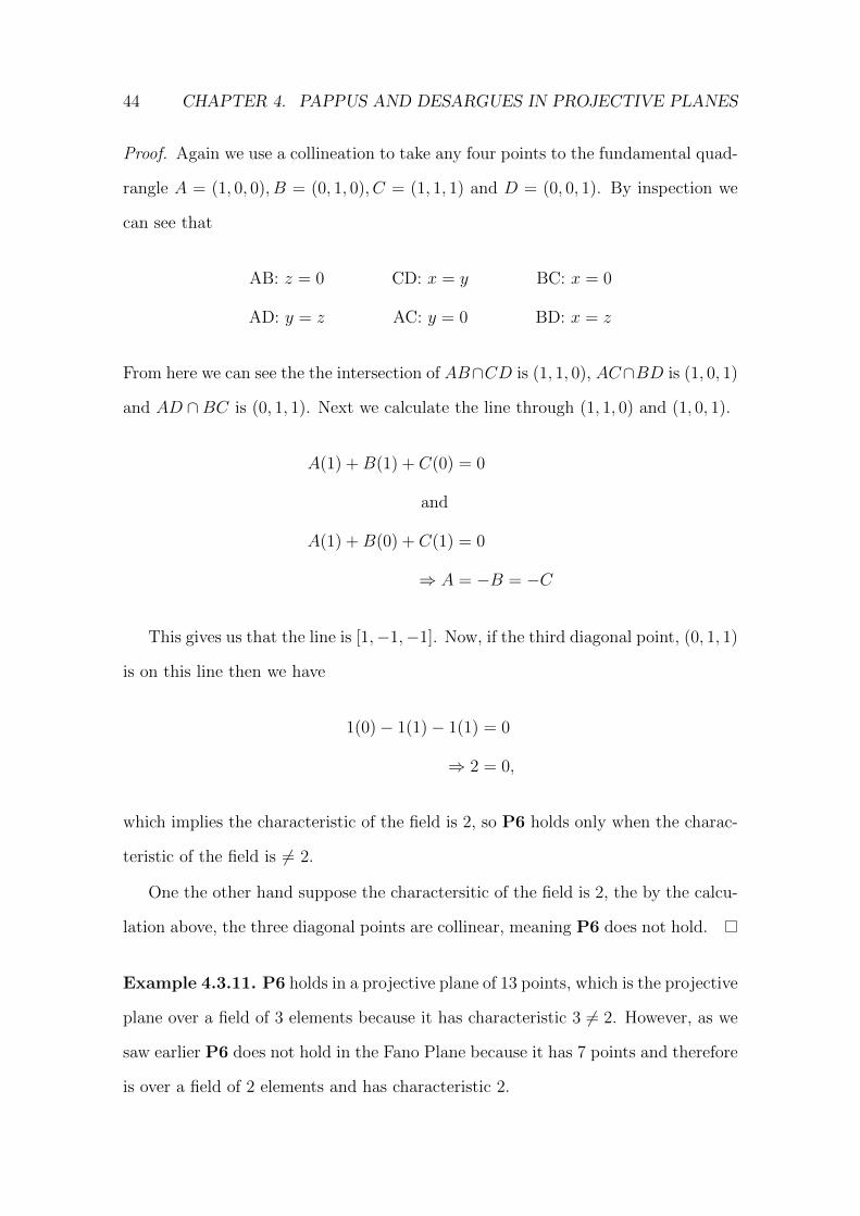
44 CHAPTER 4. PAPPUS AND DESARGUES IN PROJECTIVE PLANES
Proof. Again we use a collineation to take any four points to the fundamental quad-
rangle A = (1, 0, 0), B = (0, 1, 0), C = (1, 1, 1) and D = (0, 0, 1). By inspection we
can see that
AB: z = 0 CD: x = y BC: x = 0
AD: y = z AC: y = 0 BD: x = z
From here we can see the the intersection of AB∩CD is (1, 1, 0), AC∩BD is (1, 0, 1)
and AD ∩BC is (0, 1, 1). Next we calculate the line through (1, 1, 0) and (1, 0, 1).
A(1) +B(1) + C(0) = 0
and
A(1) +B(0) + C(1) = 0
⇒ A = −B = −C
This gives us that the line is [1,−1,−1]. Now, if the third diagonal point, (0, 1, 1)
is on this line then we have
1(0)− 1(1)− 1(1) = 0
⇒ 2 = 0,
which implies the characteristic of the field is 2, so P6 holds only when the charac-
teristic of the field is 6= 2.
One the other hand suppose the charactersitic of the field is 2, the by the calcu-
lation above, the three diagonal points are collinear, meaning P6 does not hold.
Example 4.3.11. P6 holds in a projective plane of 13 points, which is the projective
plane over a field of 3 elements because it has characteristic 3 6= 2. However, as we
saw earlier P6 does not hold in the Fano Plane because it has 7 points and therefore
is over a field of 2 elements and has characteristic 2.

4.3. ALGEBRAIC CONSEQUENCES 45
The algebraic consequences of geometric propositions are outlined in Figure 4.11.
In this form, it is easy to see the clear correlation between the geometric and algebraic
hierarchies, for example every Pappian plane is Desarguesian because every field is a
division ring. Note however that D10, D9, P9 etc. include more conditions on points
and lines which must be satisfied, suggesting they are stronger theorems but in fact
they imply weaker algebraic conditions.
P9/dP9
D9
D10
Desargues
Pappus
field
division ring
alternative division ring
⇒ if ab = 1 then ba = 1 and for all x,
(xa)b = b(ax) = x
⇒ associative and commutative addition/
additive and multiplicative inverses
Figure 4.11: Corresponding algebraic conditions
Of course, in the finite case things look quite different. In fact, they are much
simpler thanks to a few results given below. Firstly we will use Wedderburn’s
Theorem, sometimes also referred to as Little Wedderburn’s Theorem, from 1905.
It is a very famous algebraic result for which many different proofs can easily be
found. Secondly we use the Artin-Zorn Theorem from 1930 which is a generalization

46 CHAPTER 4. PAPPUS AND DESARGUES IN PROJECTIVE PLANES
of Wedderburn’s Theorem.
Theorem 4.3.12 (Wedderburn’s Theorem 1905). Every finite division ring is com-
mutative and therefore a field.
Corollary 4.3.13. Any finite projective plane which is Desarguesian is also Pap-
pian.
Proof. By Theorem 4.3.1, any projective plane which is Desarguesian is isomorphic
to PG(2, D). However in the finite case D will also be a field so by Theorem 4.3.5 any
plane which is isomorphic to PG(2, D) is also Pappian, meaning they are equivalent.
Theorem 4.3.14 (Artin-Zorn Theorem 1930). Any finite alternative division ring
is a field.
Corollary 4.3.15. A finite Moufang Plane is Desarguesian.
Proof. A Moufang plane is equivalent to the vector space being over an alternative
division ring. By the Artin-Zorn theorem a finite Moufang plane is equivalent to
a vector space over a field which by Theorem 4.3.5 is Pappian and therefore also
Desarguesian.
Lemma 4.3.16 (Reidemeister [19]). In a finite projective plane P9 and dP9 are
equivalent.
Theorem 4.3.17 (Luneburg 1960 [12]). A finite projective plane satisfying either
version of Little Pappus’ Theorem is Pappian.
Remark. This result is due to Heinz Luneburg in 1960. Luneburg proved that
a finite projective plane is Desrguesian if it satisfies: a) the Little Reidemeister
Condition, which is weaker than the full Reidemeister Condition and only implies
the associative properties of the additive loop of the planar ternary rings which

4.3. ALGEBRAIC CONSEQUENCES 47
coordinatise the plane, instead of the ternary rings themselves, and b) Axial Lit-
tle Pappus’ Theorem. However by Theorem 4.2.3, in a finite projective plane the
Reidemeister Condition and subsequently the Little Reidemeister Condition follow
from Axial Little Pappus, meaning condition a) above follows from condition b).
Since Central and Axial Little Pappus are equivalent in a finite projective plane, it
follows from Luneburg’s Theorem that a finite projective plane is Desarguesian if it
satisfies either version of Little Pappus’ Theorem. Since a finite Desarguesian plane
is also Pappian by Corollary 4.3.13 we have that in the finite case Little Pappus
implies Pappus.
Therefore we have a collapsing of our theorem hierarchy as they become equiv-
alent to one another which is shown in Figure 4.12.
Pappus Desargues
Little PappusD10
Figure 4.12: Relationships between geometric propositions in finite projective planes
So far we have discussed the algebraic consequences of the geometric properties
on the planar ternary rings that can be used to coordinatise them. However, pro-
jective planes can also be classified by the algebraic structure of their collineation
groups.
Example 4.3.18. A plane is Desarguesian if it is (V, `)-transitive and a Moufang
Plane if every line is a translation line.
This method of classification is not our focus, but a full treatment can be found
in Piper and Hughes [9].

48 CHAPTER 4. PAPPUS AND DESARGUES IN PROJECTIVE PLANES
4.4 Non-Desarguesian Projective Planes
We will now give some examples of both finite and infinite non-Desarguesian pro-
jective planes.
Example 4.4.1. The first finite non-Desarguesian plane was discovered by Oswald
Veblen and Joseph Wedderburn in 1907, it has order 9.
Theorem 4.4.2 (Hall 1956 [5]). All non-Desarguesian projective planes have order
at least 9.
Remark. No proof is given, instead we refer the reader to the work of Marshall
Hall. In 1943, Hall generalised Veblen and Wedderburn’s plane of order 9 into an
infinite family of non-Desarguesian projective planes. Then, in 1956 he proved the
uniqueness of the projective plane of order 8 [5]. Since projective planes of orders
less than 8 had already been shown to be unique (apart from the projective plane
of order 6 which does not exist) and Desarguesian, Hall’s paper also proves that 9
is the smallest possible order of a non-Desarguesian projective plane.
There are also infinite non-Desarguesian projective planes. Perhaps the first class
to come to mind is the infinite Moufang planes since we know that D10 does not
imply Desargues, thanks to the existence of a counterexample.
Example 4.4.3. The projective plane over the octonions is an infinite projective
plane which is non-Desarguesian.
More generally infinite alternative rings are not division rings and since Desar-
gues can be shown to be equivalent to associative multiplication, it is clear that
Desargues will not hold in an infinite Moufang plane.
Our last example dates back to the work of David Hilbert. In his Grundlagen
der Geometrie, Hilbert proved that axioms P1-P4 are a consequence of Desargues’
Theorem however the converse is not true [7]. To show that Desargues’ Theorem is

4.4. NON-DESARGUESIAN PROJECTIVE PLANES 49
−4 −2 2 4 6 8 10 12 14 16 18 20 22 24
−6
−4
−2
2
4
6
8
10
12
Figure 4.13: The Moulton Plane
not a consequence of the plane axioms, he set out to construct a non-Desarguesian
projective plane. However, his synthetic counterexample is far more complicated
than necessary. In 1902, Forest Ray Moulton, with the same objective, proposed
a much simpler construction of an infinite plane which does not satisfy Desargues’
Theorem [15]. It is now called the Moulton Plane after him.
Example 4.4.4. The Moulton Plane is made by taking the real affine plane and
adding a line at infinity to make it a projective plane. The points are simply the
points of R2. The horizontal, vertical lines as well as the lines with negative gradient
remain the same while the lines with positive gradient are refracted by a factor of 2
at the x-axis. A picture of some lines in the Moulton Plane is given in Figure 4.13.
It is not immediately obvious that the Moulton Plane is in fact still a projective
plane. We will prove it satisfies P1, P2 is shown in a similar manner and P3 and
P4 are trivial.
Claim 4.4.5. The Moulton Plane satisfies P1.
Proof. To show that for every pair of distinct points there exists a unique line that is

50 CHAPTER 4. PAPPUS AND DESARGUES IN PROJECTIVE PLANES
−4 −2 2 4 6 8 10 12 14 16 18 20 22 24
−6
−4
−2
2
4
6
8
10
12
A
B
C
D
E
F
GH
I
J
Figure 4.14: Desargues’ Theorem fails in the Moulton Plane
incident to both, the only case we need to consider is when the two points straddle
the x-axis, and the one above is to the right of the one below, otherwise P1 is
satisfied by the fact that PR2 is a projective plane. Let A be a point below the
x-axis and let B a point above the x-axis to the right of A. Let ` be a line through
A and B with gradient l1 below the x-axis and l2 above. Suppose m is a line through
A with gradient m1 below the x-axis and m2 above. If m1 > l1 then that value of
the x-intercept of m will be less than that of ` and m2 > l2 meaning m and ` cannot
intersect above the x-axis. Hence, if B lies on `, m cannot pass through B, instead
m will pass to the left of B. Similar logic can be used to show that m will pass to
the right of B if m1 < l1. Therefore m will pass through B if and only if m1 = l1
and m2 = l2 meaning m = `.
Lemma 4.4.6. P6 holds in the Moulton Plane.
Proof. The Moulton Plane can be coordinatised by the real numbers, a field of
characteristic 6=2, so by Theorem 4.3.10 it is a Fano Plane.

4.4. NON-DESARGUESIAN PROJECTIVE PLANES 51
Theorem 4.4.7 (Kadison and Kromann, Section 8.4 [10]). P6 and Desargues’
Theorem are independent of one another.
Proof. The Moulton plane satisfies P6 but is non-Desarguesian. A projective plane
over a division ring is a Desarguesian plane which does not satisfy P6.. Therefore
neither can imply the other meaning they are independent.
Theorem 4.4.8 (Kadison and Kromann, Section 8.4 [10]). P6 and Pappus’ Theo-
rem are independent of one another.
Proof. Since the Moulton plane is non-Desarguesian by Theorem 4.2.1 which says
that all Pappian planes are Desarguesian, the Moulton Plane is also non-Pappian.
Therefore in the Moulton plane P6 holds but not Pappus’ Theorem. Meanwhile,
Pappus’ Theorem holds in the Fano Plane but P6 does not. Again, neither can
imply the other meaning the are independent.

Chapter 5
Bricard’s Theorem
5.1 Bricard from Desargues
We now introduce a new geometric proposition which is the focus of this thesis. The
proposition is known as Bricard’s Theorem, as it was originally studied in the real
plane where it is always true. It is attributed to Raoul Bricard and traditionally
thought to appear first in his book Geometrie Descriptive, published in 1911 [2],
although several searches by myself and my supervisors have failed to find it. How-
ever, all works citing Bricard’s Theorem still reference this book, so we shall too.
In fact, there has been very little investigation of Bricard’s Theorem since it was
published and it appears in very few papers. It seems that everywhere it appears,
no assumptions are given about the underlying structure of the projective plane. Is
it PG(2, D)? Is it PG(2, F )? Is it a direct consequence of P1-P4 and therefore holds
in every projective plane? Only Bamberg and Penttila clarify they are working in
PG(2, D) when giving a proof of Bricard’s Theorem (private communication, 2021).
The theorem is given in two directions BI and BII as we cannot assume they are
equivalent. Bamberg and Penttila show one direction, we follow their approach to
prove both directions.
52
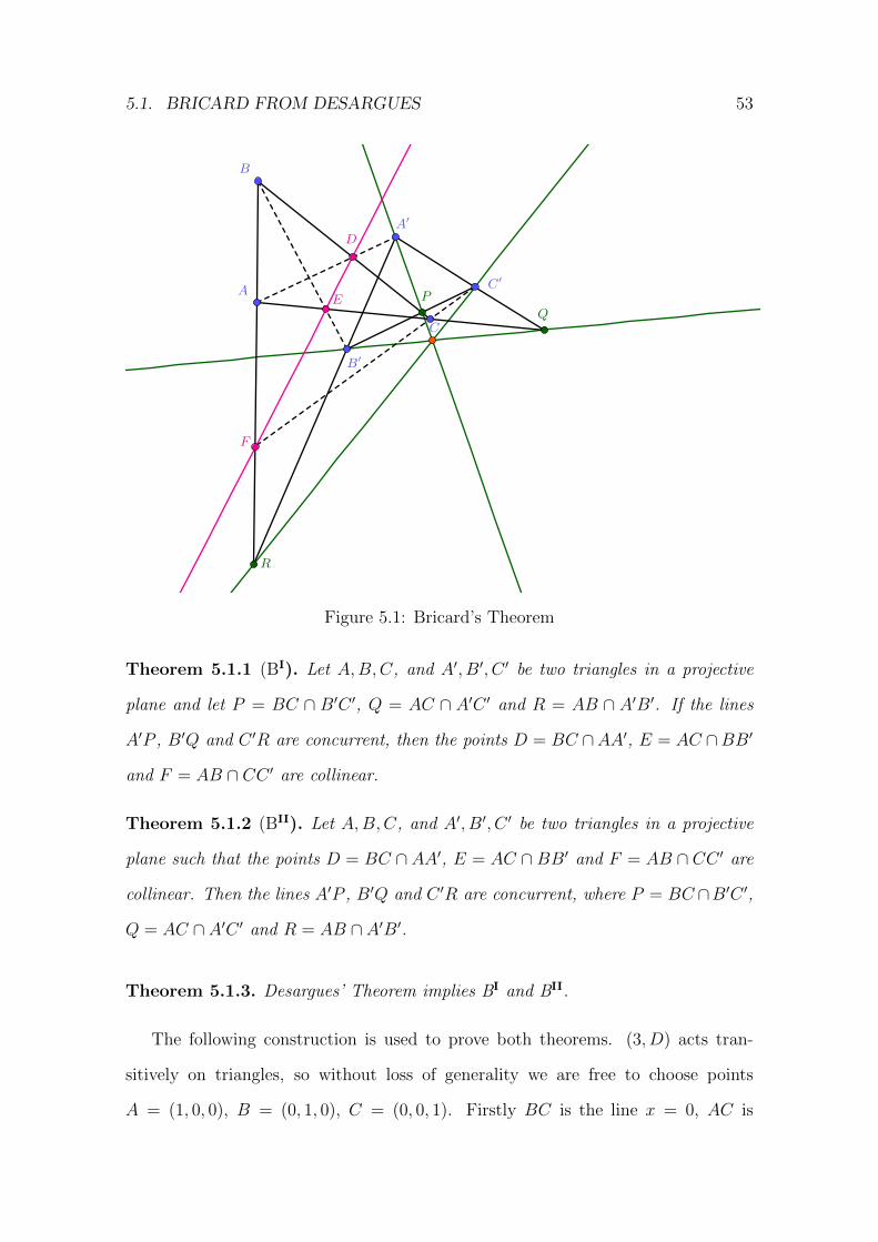
5.1. BRICARD FROM DESARGUES 53
A
B
C
A′
B′
C′
E
D
F
P
Q
R
Figure 5.1: Bricard’s Theorem
Theorem 5.1.1 (BI). Let A,B,C, and A′, B′, C ′ be two triangles in a projective
plane and let P = BC ∩ B′C ′, Q = AC ∩ A′C ′ and R = AB ∩ A′B′. If the lines
A′P , B′Q and C ′R are concurrent, then the points D = BC ∩AA′, E = AC ∩BB′
and F = AB ∩ CC ′ are collinear.
Theorem 5.1.2 (BII). Let A,B,C, and A′, B′, C ′ be two triangles in a projective
plane such that the points D = BC ∩ AA′, E = AC ∩ BB′ and F = AB ∩ CC ′ are
collinear. Then the lines A′P , B′Q and C ′R are concurrent, where P = BC ∩B′C ′,
Q = AC ∩ A′C ′ and R = AB ∩ A′B′.
Theorem 5.1.3. Desargues’ Theorem implies BI and BII.
The following construction is used to prove both theorems. (3, D) acts tran-
sitively on triangles, so without loss of generality we are free to choose points
A = (1, 0, 0), B = (0, 1, 0), C = (0, 0, 1). Firstly BC is the line x = 0, AC is

54 CHAPTER 5. BRICARD’S THEOREM
the line y = 0 and AB is the line z = 0.
Let the line through DF be [1, 1, 1]. D = (d1, d2, d3) is on [1, 1, 1] and [1, 0, 0] so
d1 + d2 + d3 = 0 and d1 = 0
⇒ D = (0,−1, 1).
Similarly, F = (f1, f2, f3) is on [1, 1, 1] and [0, 0, 1] so
f1 + f2 + f3 = 0 and f3 = 0
⇒ F = (−1, 1, 0).
Now that we have the points D and F , we can calculate the lines AD =
[AD|1, AD|2, AD|3] and CF = [CF |1, CF |2, CF |3].
AD|1(1) = 0 (A on AD)
AD|2(−1) + AD|3(1) = 0 (D on AD)
⇒ AD = [0, 1, 1].
CF |3(1) = 0 (C on CF )
CF |1(−1) + CF |2(1) = 0 (F on CF )
⇒ CF = [1, 1, 0].
Since A′ is a point on AD not equal to D, we can say A′ = (α, 1,−1) for some α.
In the same way C ′ is a point on CF not equal to C so C ′ = (1,−1, γ) for some γ.
We can now calculate the line A′C ′ = [A′C ′|1, A′C ′|2, A′C ′|3].
0 = A′C ′|1(α) + A′C ′|2(1) + A′C ′|3(−1) (A′ on A′C ′)(3)
= A′C ′|1(1) + A′C ′|2(−1) + A′C ′|3(γ) (C ′ on A′C ′)(4)
= A′C ′|1 + A′C ′|1(α) + A′C ′|3(γ)− A′C ′|3 (add 3 and 4)
= A′C ′|1(α + 1) + A′C ′|3(γ − 1)(5)

5.1. BRICARD FROM DESARGUES 55
Recall the definition of Q = AC ∩ A′C ′, so Q = (q1, q2, q3) is the intersection of
A′C ′ and [0, 1, 0],
q2 = 0
⇒ A′C ′|1(q1) + A′C ′|3(q3) = 0
⇒ Q = (α + 1, 0, γ − 1) (by 5)
We cannot yet find R or P explicitly but we know that R lies on AB, which is
the line z = 0, so we can say R is of the form (r1, r2, 0), and P lies on BC which is
the line x = 0 so P must be of the form (0, p2, p3).Now the line A′R has:
0 = A′R|1α + A′R|2 − A′R|3 (A′ on A′R)(6)
= A′R|1r1 + A′R|2r2 (R on A′R)(7)
= A′R|1(r1 − α) + A′R|2(r2 − 1) + A′R|3 (7 subtract 6)(8)
By the definition of R, B′ lies on A′R so by (8) we can say the B′ = (r1−α, β, 1),
where β = r2 − 1, which also implies that r2 = β + 1 which gives R = (r1, β + 1, 0).
Lastly, we need to find the point P using the fact that P is the intersection of BC
and B′C ′. The line B′C ′ = [B′C ′|1, B′C ′|2, B′C ′|3] has:
0 = B′C ′|1(r1 − α) +B′C ′|2(β) +B′C ′|3(1) (B′ on B′C ′)(9)
= B′C ′|1(1) +B′C ′|2(−1) +B′C ′|3(γ) (C ′ on B′C ′)(10)
= B′C ′|1(r1 − α + 1)−B′C ′|2(β − 1) +B′C ′|3(γ + 1) (add 9 and 10)
So P is the intersection of this line with x = 0. We now write equations for the
lines A′P,B′Q and C ′R. A′P = [A′P |1, A′P |2, A′P |3] has:
0 = A′P |1(α) + A′P |2(1) + A′P |3(−1) (A′ on A′P )(11)
= A′P |2(p2) + A′P |3(p3) (P on A′P )(12)
= A′P |1α + A′P |2(1 + p2) + A′P |3(p3 − 1) (add 11 and 12)

56 CHAPTER 5. BRICARD’S THEOREM
B′Q = [B′Q|1, B′Q|2, B′Q|3] has:
0 = B′Q|1(α + 1) +B′Q|3(γ − 1) (Q on B′Q)(13)
= B′Q|1(r1 − α) +B′Q|2β +B′Q|3(1) (B′ on B′Q)(14)
= B′Q|1(r1 + 1) +B′Q|2β +B′Q|3γ (add 13 and 14)
C ′R = [C ′R|1, C ′R|2, C ′R|3] has:
0 = C ′R|1(1) + C ′R|2(−1) + C ′R|3(γ) (C ′ on C ′R)(15)
= C ′R|1(r1) + C ′R|2(β + 1) (R on C ′R)(16)
= C ′R|1(r1 + 1) + C ′R|2β + C ′R|3γ (add 15 and 16)
A′P: A′P |1α + A′P |2(1 + p2) + A′P |3(p3 − 1) = 0
B′Q: B′Q|1(r1 + 1) +B′Q|2β +B′Q|3γ = 0
C′R: C ′R|1(r1 + 1) + C ′R|2β + C ′R|3γ = 0
Proof. (BI) If these three lines are concurrent then A′P must pass through (r1 +
1, β, γ), the unique point of intersection of B′Q and C ′R. Therefore α = r1 + 1
meaning r1 = α− 1 which leads to B′ = (−1, β, 1).Now the line BB′ has
0 = BB′|1(−1) +BB′|2β +BB′|3(1) (B′ on BB′)
0 = BB′|2 (B on BB′)
⇒ BB′ = [1, 0, 1]
So E = (e1, e2, e3), which is the intersection of BB′ and AC, is on [1, 0, 1] and
y = 0, so
e1 + e3 = 0 and e2 = 0
⇒ E = (−1, 0, 1).
Lastly 1(−1) + 1(0) + 1(1) = 0 so E must be on the line [1, 1, 1], meaning D,E
and F are collinear.
5.1. BRICARD FROM DESARGUES 57
Proof. (BII) If DE and F are collinear, then E lies on [1, 1, 1],
If E = (e1, e2, e3) lies on [1, 1, 1] and [0, 1, 0] we get that:
e1 + e2 + e3 = 0 and e2 = 0
⇒ E = (−1, 0, 1).
So the line BE = [BE|1, BE|2, BE|3] has
BE|2(1) = 0 (B on BE)
BE|1(−1) +BE|3(1) = 0 (E on BE)
⇒ BE = [1, 0, 1].
Using the same argument as before, B′ is a point of BE not equal to B so
B′ = (−1, β, 1). Earlier we said that B = (r1−α, β, 1) which implies that r1−α = −1
therefore r1 = α− 1. Recall that P is the intersection of B′C ′ and [1, 0, 0],
B’C’: 0 = B′C ′|1(r1 − α + 1)−B′C ′|2(β − 1) +B′C ′|3(γ + 1)
= B′C ′|1(0)−B′C ′|2(β − 1) +B′C ′|3(γ + 1) (sub in r1)(17)
⇒ P = (0, β − 1, γ + 1) (by 17)
We rewrite the equations for A′P,B′Q and C ′R in terms of α, β and γ:
A′P: A′P |1α + A′P |2β + A′P |3γ = 0
B′Q: B′Q|1α +B′Q|2β +B′Q|3γ = 0
C′R: C ′R|1α + C ′R|2β + C ′R|3γ = 0
And it is clear to see that these three lines are concurrent in (α, β, γ).
This shows that Bricard’s Theorem holds in all projective planes defined over a
division ring. We can attribute this result to Bamberg and Penttila (private com-
munication, 2021). However, we showed with Theorem 4.3.1 that all projective
planes defined over a division ring are Desarguesian this means that Desargues’
Theorem also implies Bricard’s Theorem.

58 CHAPTER 5. BRICARD’S THEOREM
5.2 Bricard in the Moulton Plane
We now turn our attention to the converse, i.e., Bricard’s Theorem implies Desar-
gues. One thing to note about the proof of BI and BII given in the previous section
is that it doesn’t appear to need associativity. There are no instances where three
things are being multiplied together. We have already seen that Desargues’ Theorem
is the geometric equivalent of associative multiplication. Does this mean that BI
and BII are weaker and do they hold in projective planes where Desargues’ Theorem
does not?
One quick way to check this would be to see if either direction of Bricard’s
Theorem holds in the Moulton Plane, which we know is non-Desarguesian. If either
BI or BII hold in the Moulton Plane then we know immediately that they cannot
imply Desargues’ Theorem. If they don’t then we need to do further analysis. Before
attempting to prove that BI and BII do hold in the Moulton Plane, first we will look
for a counterexample of them failing. As it happens this is very easy, we simply
follow the method used to construct an example of Desargues’ Theorem failing in
the Moulton Plane. The trick is to position the entire figure such that exactly one of
the points lies below the x-axis and rotate it so that exactly one of the lines through
that point has a positive gradient.
Proposition 5.2.1. BI and BII fail in the Moulton Plane.
Proof. Firstly BII, which says that collinearity implies concurrency. Take points
A = (11, 8), B = (12, 12), C = (−2, 10), A′ = (0, 14), and B′ = (4, 6). If DEF are
collinear, then we are free to let C ′ be any point on CF . Choose C ′ = (−6, 11.6).
Recall R is the intersection of AB and A′B′. In the real plane this would be the
intersection of y = 4x−36 and y = −2x+14 which is (8.3,−2.7), call this point Rreal.
However, in the Moulton Plane the line AB is a line with positive gradient
therefore it is refracted by a factor of 2 as it crosses the x-axis. The x-intercept is

5.2. BRICARD IN THE MOULTON PLANE 59
(9, 0) so the portion of AB located below the x-axis is the line with gradient 8 which
has an x-intercept at (9, 0) also. This is the line y = 8x− 72. So, the point R is the
intersection of y = −2x+ 14 and y = 8x− 72 which is (8.6,−3.2).
Since Bricard’s Theorem holds in the real projective plane, the lines A′P , B′Q
and C ′Rreal are concurrent. It is easy to calculate that the point R is not on C ′Rreal
which means that A′P , B′Q and C ′R cannot be concurrent, in other words BII fails
in the Moulton Plane. This can be seen easily in Figure 5.3.
−8 −6 −4 −2 2 4 6 8 10 12
−4
−2
2
4
6
8
10
12
14
A
B
C
A′
B′
C ′
R
P
Q D
E
F
Figure 5.2: BII fails in the Moulton Plane
A
B
C
A′
B′
C′
R
P
Q
o
D
E
F
Figure 5.3: Close up of Figure 5.2

60 CHAPTER 5. BRICARD’S THEOREM
−4 −2 2 4 6 8 10 12 14 16 18
−4
−2
2
4
6
8
10
12
A
B
C
A′C ′
B′
P
R
Q
D
E
F
Figure 5.4: BI fails in the Moulton Plane
Next we consider BI, which says that concurrency implies collinearity. This time
take A = (12, 8), B = (13, 12), C = (2, 4), A′ = (6, 10) and C ′ = (−4, 10). In
order for A′P , B′Q and C ′R to be concurrent we must have B′ = (8.1, 5.6). Now,
recall the F is the intersection of AB with CC ′. In the real plane this would be the
intersection of y = 4x− 40 with y = −x+ 6 which is (9.2,−3.2).
However, in the Moulton Plane AB is a a line with positive gradient meaning
it is refracted by a factor of 2 as it crosses the x-axis, which is at the point (10, 0).
Therefore, the portion of AB located below the x-axis is the line with gradient 8 and
x-intercept (10, 0) which is the line y = 8x− 80. So in the Moulton Plane, the point
F is the intersection of y = −x+ 6 with y = 8x− 80 which means F = (9.6,−3.6).
From here we can calculate the position of D and E and the line which joins
them. It is then easy to show that F is not on this line, meaning D, E and F are
not collinear or in other words BI fails in the Moulton Plane. This configuration is
given in Figure 5.4.

5.3. BRICARD SUMMARY 61
5.3 Bricard Summary
To summarise what we know about Bricard’s Theorem so far, we have seen that:
1. Desargues’ Theorem implies both BI and BII.
2. As a result of point 1. BI and BII are equivalent in a Desarguesian plane.
3. Bricard’s Theorem doesn’t require associative multiplication, meaning it could
be weaker than Desargues’ Theorem.
4. Bricard’s Theorem fails in the Moulton Plane. We cannot use the Moulton
Plane as a counterexample to show Bricard does not imply Desargues.
These are all useful bits of information however we are still unable to determine
whether or not either BI or BII imply Desargues’ Theorem. In fact, we still don’t
know if they are always equivalent to one another, or only in a Desarguesian Plane.
In order to introduce a potential method of answering these questions, we turn
our attention once again to algebra. For example what is the exact algebraic sig-
nificance of Bricard’s Theorem and what happens in the finite case? Knowing the
answer to the first of these questions will almost certainly help to answer the sec-
ond. We suspect Bricard’s Theorem does not require associative multiplication
which suggests it is not equivalent to the full version of Desargues’ Theorem. What
is Desargues’ Theorem without associative multiplication? Our work on algebraic
consequences tells us that the next most likely candidate is D10, which is equivalent
to an alternative division ring, a division ring without associative multiplication.
This could mean for example that Bricard is actually equivalent to D10. If so the
picture would look like this:
Suppose there was an arrow from Bricard to Desargues. Since there is already
an arrow from Bricard to D10 then this would imply another arrow from D10 to
Desargues, however we can be certain that D10 does not imply D11 because of the
octonions. This would form a contradiction and be one way to show Bricard cannot
imply Desargues, allowing us to answer our original question.

62 CHAPTER 5. BRICARD’S THEOREM
D10Bricard
Desargues
Figure 5.5: Potential Relationship between Bricard and D10
Having a geometric proof of how Desargues’ Theorem implies Bricard would
make it easy to see whether either of the two triangles used in D11 had a vertex
lying on the side of the other which would reveal whether D10 also implies Bricard.
Then we would be well on our way to utilising the method outlined above.
One last question to ask is what is the dual of Bricard, and is Bricard equivalent
to its dual?

Chapter 6
Trilinear Polar
6.1 Trilinear Polar from Bricard
We ended the previous chapter by signalling the importance of direct geometric
proofs. However if we are looking for applications of any of these theorems in
others, one important observation to make is that the configuration of Desargues’
Theorem involves 10 points and 10 lines while Bricard’s Theorem involves 13 points
and 13 lines. This makes the task more difficult as there can be no direct correlation
between the two theorems.
Recall Pappus’ Theorem and Desargues’ Theorem both had degenerate versions
involving extra incidences between points and lines. In the case of Bricard’s theo-
rem, perhaps we can do the same thing. Ideally introducing three extra incidences
between points and other points, to reduce the number of points from 13 to 10. In
this way, we have a better chance of finding a direct link to Desargues’ Theorem or
perhaps even one of D10 or D9. This motivates the following corollary of Bricard’s
Theorem.
Theorem 6.1.1 (Trilinear Polar). Let A,B,C, and A′, B′, C ′ be two triangles in a
projective plane such that the point A lies on A′C ′, B lies on A′B′ and C lies on
B′C ′. Then the points D = BC ∩ AA′, E = AC ∩ BB′ and F = AB ∩ CC ′ are
collinear if the lines A′C, B′A and C ′B.
63

64 CHAPTER 6. TRILINEAR POLAR
B′
A′
C′
B
C
A
E F D
Figure 6.1: Trilinear Polar
As it happens this is precisely the statement given by the Trilinear Polar Theorem
attributed to J.-J.-A. Mathieu in 1865 [13]. The requirement that A lies on A′C ′,
B lies on A′B′ and C lies on B′C ′ means that P = C, Q = A and R = C.
With this we have reduced the number of points by three, meaning there are now
10 points remaining, the same number as in Desargues’ Theorem. One possible
configuration of Trilinear Polar is given in Figure 6.1 and already looks distinctly
more Desarguesian than the full version of Bricard’s Theorem, however it is still
clear to see that Trilinear Polar is a direct result of Bricard’s Theorem. As far as
we can tell this connection has not been made before.
However, the Trilinear Polar Theorem is well known and arises in a number of
other contexts. For example, another way to phrase the Trilinear Polar Theorem is
that the harmonic conjugates of C with respect to B′C ′, B with respect to A′B′ and
A with respect to A′C ′ are collinear. This statement can be proven using the cross
ratio, R(a, b, c, d) which is defined on a set of four collinear points and is invariant
under projective transformations.
R(a, b, c, d) =a− ca− d
· b− db− c
The cross ratio is a result of the theorems of Giovanni Ceva and Menelaus, which
6.2. TRILINEAR POLAR IN THE HIERARCHY 65
in the real projective plane are the dual of each other. Menelaus’ Theorem first
appears in his book Spaerica dating back to roughly 100 AD while Ceva published
his theorem in 1678. However, although it is attributed to Ceva it appears to have
been proven much earlier by Yusuf Al-Mu’taman ibn Hud, an eleventh-century king
of Zaragoza [8]. In algebraic terms, the cross ration implies we only need inverses to
commute, similar to the case for D9. However, there could also be other algebraic
consequences which are a result of Trilinear Polar.
A third way to express Trilinear Polar theorem follows. However, first we need
the definition of the Cevian triangle, named after Ceva, and the trilinear pole and
polar, from which the theorem gets its name.
Definition 6.1.2 (Cevian Triangle). Given a triangle ABC and a point P the
cevian triangle is defined as the triangle with verticesD = AP∩BC, E = BP∩AC
and F = CP∩AB. A triangle and its cevian are always in perspective from the point
P which is referred to as the trilinear pole while the line through the intersections
of corresponding sides is called the trilinear polar.
With this definition in mind we can can restate the Trilinear Polar theorem as
follows: The intersections of the corresponding sides of a triangle and it’s cevian are
collinear. When phrased like this is is easy to see that Trilinear Polar is a direct
consequence of Desargues Theorem (because the two triangles are always centrally
perspective) but also D10 and D9 as well. Trilinear Polar can also be thought of as
D8, or Desargues with three extra incidences.
6.2 Trilinear Polar in the Hierarchy
Theorem 6.2.1. Special Desargues implies Trilinear Polar.
Proof. Let ABC, and A′B′C ′ be two triangles in a projective plane such that the
point A lies on A′C ′, B lies on A′B′ and C lies on B′C ′ and the lines A′C, B′A and

66 CHAPTER 6. TRILINEAR POLAR
C ′B are concurrent. In other words they are centrally perspective from a point P .
We want to show the points D = BC ∩ AA′, E = AC ∩ BB′ and F = AB ∩ CC ′
are collinear. Note that we have two triangles in perspective from a point such that
one triangle has a vertex lying on a side of the other. So by Special Desargues
the intersections of their corresponding sides are collinear. That is, AB ∩ B′C ′,
AC ∩A′C ′ and BC ∩A′C ′ are concurrent. But C lies on B′C ′ by definition so B′C ′
is the same line as CC ′. Using the same argument A′C ′ is the same line as AA′ and
A′B′ is the same line as BB′. Now we have BC ∩ AA′, AC ∩ BB′ and AB ∩ CC ′
are collinear which is precisely the points D, E and F .
Theorem 6.2.2. D9 implies Trilinear Polar.
Remark. The proof is almost identical to the one above, but instead we have
one triangle with two vertices lying on two sides of the other triangle, so we are able
to use the proposition of D9 to show that the intersections of corresponding sides
are collinear.
Theorem 6.2.3. Central Little Pappus plus P6 implies Trilinear Polar.
Proof. Given triangle ABC and a point P , construct the cevian triangle DEF where
D = AP∩BC, E = BP∩AC and F = CP∩AB. Let X = BC∩EF , Y = AC∩DF
and Z = AB ∩ DE. We want to show X, Y and Z are collinear. Consider lines
AF and CD which meet at B. The intersection of CF and AD is the point P . The
intersection of DZ and FX is E because X is on EF and Z is on ED. We also
know that B, E and P are collinear because we constructed E to be that way. By
Little Pappus’ Theorem to show that V = AX ∩ CZ is also collinear with B, E
and P . By the same argument U = BY ∩ CZ is collinear with A, P and D and
W = AX ∩BY is collinear with C, P and F .
Now consider the three collinear points A, C and Y , and the point V . The line
UW is a line through Y which meets V C in U and V A in W . The intersection of
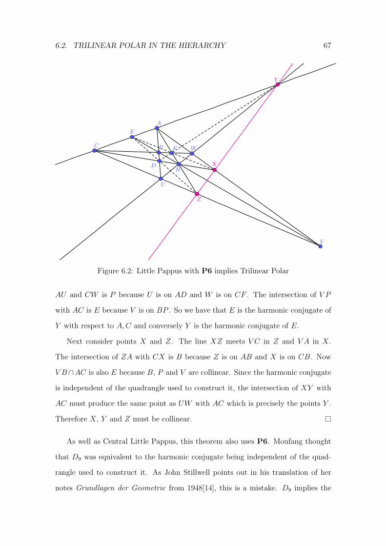
6.2. TRILINEAR POLAR IN THE HIERARCHY 67
A
C
B
P
E
D
F W
Y
X
U
Z
V
Figure 6.2: Little Pappus with P6 implies Trilinear Polar
AU and CW is P because U is on AD and W is on CF . The intersection of V P
with AC is E because V is on BP . So we have that E is the harmonic conjugate of
Y with respect to A,C and conversely Y is the harmonic conjugate of E.
Next consider points X and Z. The line XZ meets V C in Z and V A in X.
The intersection of ZA with CX is B because Z is on AB and X is on CB. Now
V B∩AC is also E because B, P and V are collinear. Since the harmonic conjugate
is independent of the quadrangle used to construct it, the intersection of XY with
AC must produce the same point as UW with AC which is precisely the points Y .
Therefore X, Y and Z must be collinear.
As well as Central Little Pappus, this theorem also uses P6. Moufang thought
that D9 was equivalent to the harmonic conjugate being independent of the quad-
rangle used to construct it. As John Stillwell points out in his translation of her
notes Grundlagen der Geometrie from 1948[14], this is a mistake. D9 implies the

68 CHAPTER 6. TRILINEAR POLAR
harmonic conjugate is in fact independent of the quadrangle used to construct it
however the converse is not true, that is if the harmonic conjugate is independent of
the quadrangle used to construct it, D9 does not necessarily hold. This is important
as otherwise Little Pappus on its own would not imply trilinear polar, we would
also be using D9 as well. D9 is actually equivalent to the harmonic conjugate being
unique, which is a stronger property than P6 or equivalently that the harmonic con-
jugate of a point is never equal to itself. The uniqueness of the harmonic conjugate
is proven by Seidenberg in [21] while proof that D9 is equivalent to the harmonic
conjugate being unique can be found in Heyting, Theorem 2.4.3 [6].
Theorem 6.2.4. D9 implies BI with two pairs of coincident points.
Proof. Let H, I and J be three distinct points in a projective plane. Let A, B, C,
A′, B′, and C ′ be distinct points such that 1) AA′ ∩ BB′ = I, AA′ ∩ CC ′ = J and
BB′ ∩ CC ′ = H and 2) A′P , B′Q and C ′R are concurrent, where P = BC ∩B′C ′,
Q = AC ∩ A′C ′ and R = AB ∩ A′B′. We want to show the points D = BC ∩ AA′,
E = AC ∩BB′ and F = AB ∩ CC ′ are collinear.
The first condition implies that AA′ = IJ , BB′ = HI and CC ′ = HJ . Now we
have that D = BC ∩ IJ , E = AC ∩HI and F = AB ∩HJ . Assuming D9 holds,
Trilinear Polar also holds and D, E and F will be collinear if one of triangles ABC
or HIJ is the cevian of the other. If A′ = I, B′ = H and C ′ is any point on HJ ,
then
R = AB ∩ A′B′ = AB ∩HI = B
P = BC ∩B′C ′ = BC ∩HJ = C
Let L = QP ∩A′B′. The second condition means A′P , B′Q and C ′R are concurrent,
so R is the harmonic conjugate of L with respect to A′, B′. Now D9 is equivalent
to the uniqueness of the harmonic conjugate. If we change the quadrangle we must
still get the same harmonic conjugate. Recall A′ = I and B′ = H, we can see that
6.2. TRILINEAR POLAR IN THE HIERARCHY 69
AC = QP because Q is on AC and IA ∩HC = J . Let K = CI ∩ AH, RK must
go through J , but R = B so BK goes through J , meaning IC, HA and JB are
concurrent. Also since A is on IJ , B is on HI and C is on HJ , ABC is the cevian
of HIJ .
Conjecture 1. Neither BI nor BII imply Desargues.
Remark. We have discovered evidence to suggest that Bricard’s Theorem is
actually far more closely related to Trilinear Polar than it is to Desargues’ Theorem.
In light of Theorem 6.2.4, we conjecture that it is equivalent to D9, however we have
not yet proven this equivalence without extra conditions on the points of Bricard’s
Theorem. Since it is known that D10 does not imply Desargues’ Theorem, it follows
that no theorem that sits beneath it in the hierarchy does either. Therefore if
Bricard’s Theorem is equivalent to any of the three listed above, it does not imply
Desargues’ Theorem.

Chapter 7
Concluding Remarks
Geometric propositions are a wonderful tool for classifying projective planes. Indeed
some of them, including the theorems of Pappus and Menelaus have been around
since long before the idea projective geometry was conceived. Although many of
them can be depicted by a simple diagram consisting of 10 or so points and lines, we
have discovered that the relationships between them are actually rather complex.
We have provided a summary of the known relationships between Pappus’ Theorem,
Desargues’ Theorem, Fano’s Axiom and the Reidemeister condition. Beginning in
1905 with Hessenberg’s incomplete proof, relationships between these theorems were
explored throughout the 20th century. However, there remain some intriguing open
questions regarding versions of these theorems involving extra incidences between
points and lines. A list is complied below.
• D9 is equivalent to D10 is a Fano Plane, but is this true in general?
• Are all possible configurations of Desargues’ Theorem with two extra inci-
dences equivalent?
• Does either P9 or dP9 imply D9?
• Are P9 and dP9 equivalent?
70

71
In addition to the relationships between geometric propositions, we also gave
a brief overview of the algebraic conditions on the planar ternary rings that are
implied by them. A clear correspondence can be seen between the hierarchy of the
geometric propositions and their underlying algebraic structures. This alludes to
the fact that geometry and algebra are inherently entwined.
Lastly, we attempted to introduce Bricard’s Theorem, another less well known
geometric proposition from the early 20th century, into the classification. Initially
motivated by the question ‘Does Bricard’s Theorem imply Desargues’ Theorem, we
uncovered the central role played by Trilinear Polar, yet another geometric propo-
sition, published in 1865 but overlooked by both Moufang and Heyting.
It appears that Trilinear Polar is the weakest of the propositions and is implied
by all of the others. An exploration of the relationship between Trilinear Polar and
Bricard led us to prove that D9 implies Bricard’s Theorem in the case where two
pairs of points from Bricard overlap (condition (1) in Figure 7.1), however we have
also discovered strong evidence to suggest the condition can be removed and the
implication will still hold. This leads us to the conjecture that Bricard’s Theorem
is equivalent to D9. For this reason, we suspect Bricard’s Theorem does not imply
Desargues’ Theorem because the octonions are a counterexample proving Desargues’
Theorem is not equivalent to any weaker geometric proposition, however there is still
a lot more research to be done on Bricard’s Theorem.
Additional relationships between geometric properties presented in this thesis are
summarised in Figure 7.1. In this case, P6 is taken as an axiom of the projective
plane to simplify the graph. Once again an arrow means ‘implies’, no arrow means
‘does not imply’ and a dotted arrow suggests it is still an open problem. Arrows in
red indicate original work. Algebraic consequences are summarised in Figure 7.2,
where the dotted rectangle represents the placement of Bricard as suggested by our
research.

72 CHAPTER 7. CONCLUDING REMARKS
D10BI
Pappus
Desargues
P9
dP9
BII
D9
Trilinear Polar
(1)
+VW*
Figure 7.1: Summary of Relationships in a Fano Plane

73
Trilinear Polar
Little Pappus
D9
D10
Desargues
Pappus
BI/
BII?
field
division ring
alternative division ring
⇒ if ab = 1 then ba = 1 and for all x,
(xa)b = b(ax) = x
⇒ associative and commutative addition/
additive and multiplicative inverses
⇒ if ab = 1 then ba = 1
Figure 7.2: Summary of algebraic consequences

Bibliography
[1] A. Bosse. Maniere universelle de Mr. Desargues pour pratiquer la perspective.
1648.
[2] R. Bricard. Geometrie Descriptive. Octave Doin et Fils, 1911.
[3] L. Da Vinci and H. Suh. Leonardo’s Notebooks: Writing and Art of the Great
Master. Notebook Series. Running Press, 2013.
[4] M. Hall. Projective planes. Trans. Amer. Math. Soc., 54:229–277, 1943.
[5] M. Hall, J. Swift, and R. J. Walker. Uniqueness of the projective plane of order
eight. Mathematics of Computation, 10:186–194, 1956.
[6] A. A. Heyting. Axiomatic projective geometry. Bibliotheca mathematica, a
series of monographs on pure and applied mathematics ; v. 5. P. Noordhoff,
Groningen, 2d ed. edition, 1980.
[7] D. Hilbert. Grundlagen der Geometrie. Vieweg+Teubner Verlag, 13 edition,
1968.
[8] A. Holme. Geometry Our Cultural Heritage. Springer Berlin Heidelberg, Berlin,
Heidelberg, 2nd ed. 2010. edition, 2010.
[9] D. Hughes and F. Piper. Projective Planes. Graduate texts in mathematics.
Springer-Verlag, 1973.
[10] L. Kadison. Projective geometry and modern algebra. Birkhauser, Boston, 1996.
[11] M. Kallaher. Reidemeister projective planes. 1967.
[12] H. Luneburg. Uber die beiden kleinen satze von pappos. Archiv der Mathematik,
11:339–341, 1960.
74
BIBLIOGRAPHY 75
[13] J.-J.-A. Mathieu. Etude de geometrie comparee, avec applications aux sections
coniques. Nouvelles annales de mathematiques : journal des candidats aux
ecoles polytechnique et normale, pages 529–537, 1865.
[14] R. Moufang and J. Stillwell. Translation of moufang’s‘grundlagen der geome-
trie’, 2020.
[15] F. R. Moulton. A simple non-desarguesian plane geometry. Transactions of the
American Mathematical Society, 3:192–195, 1902.
[16] Pappus of Alexandria. Pappus of Alexandria Book 7 of the Collection. Springer-
Verlag New York, 1 edition, 1986.
[17] G. Pickert. Projektive Ebenen. Springer, Berlin, Heidelberg, 2 edition, 1975.
[18] J.-V. Poncelet. Traite des proprietes projectives des figures. L’ecole Imperiale
Polytechnique, 2 edition, 1865.
[19] K. Reidemeister. Topologische Fragen der Differentialgeometrie. V. Gewebe und
Gruppen, volume 29. 1929.
[20] A. Seidenberg. Pappus implies desargues. The American Mathematical
Monthly, 83(3):190–192, 1976.
[21] A. A. Seidenberg. Lectures in projective geometry. The University series in
undergraduate mathematics. Van Nostrand, Princeton, N.J, 1962.
[22] J. Stillwell. The four pillars of geometry. Undergraduate texts in mathematics.
Springer, New York, 2005.
[23] O. Veblen and J. Young. Projective Geometry. Number v. 1 in Projective
Geometry. Ginn, 1910.