A Resource Cost Aware Cumulative

Helmut Simonis and Tarik Hadzic?

Cork Constraint Computation CentreDepartment of Computer Science, University College Cork, Ireland

{h.simonis,t.hadzic}@4c.ucc.ie

Abstract. We motivate and introduce an extension of the well-known cumula-tive constraint which deals with time and volume dependent cost of resources.Our research is primarily interested in scheduling problems under time and vol-ume variable electricity costs, but the constraint equally applies to manpowerscheduling when hourly rates differ over time and/or extra personnel incur higherhourly rates. We present a number of possible lower bounds on the cost, includinga min-cost flow, different LP and MIP models, as well as greedy algorithms, andprovide a theoretical and experimental comparison of the different methods.

1 Introduction

The cumulative constraint [1, 2] has long been a key global constraint allowing theeffective modeling and resolution of complex scheduling problems with constraint pro-gramming. However, it is not adequate to handle problems where resource costs changewith time and use, and thus must be considered as part of the scheduling. This problemincreasingly arises with electricity cost, where time variable tariffs become more andmore widespread. With the prices for electricity rising globally, the contribution of en-ergy costs to total manufacturing cost is steadily increasing, thus making an effectivesolution of this problem more and more important. Figure 1 gives an example of thewhole-sale price in the Irish electricity market for a sample day, in half hour intervals.Note that the range of prices varies by more than a factor of three, and the largest dif-ference between two consecutive half-hour time periods is more than 50 units. Hence,large cost savings might be possible if the schedule of electricity-consuming activitiestakes that cost into account.

The problem of time and volume dependent resource cost equally arises in man-power scheduling, where hourly rates can depend on time, and extra personnel typi-cally incurs higher costs. We suggest extending the standard CP scheduling frameworkto variable resource cost scenarios by developing a cost-aware extension of the cu-mulative constraint, CumulativeCost. The new constraint should support both thestandard feasibility reasoning as well as reasoning about the cost of the schedule. As afirst step in this direction we formally describe the semantics of CumulativeCostand discuss a number of algorithms for producing high quality lower-bounds (used forbounding or pruning during optimization) for this constraint. The proposed algorithmsare compared both theoretically and experimentally. Previous research on the cumula-tive constraint has focused along three lines: 1) improvement of the reasoning methods? This work was supported by Science Foundation Ireland (Grant Number 05/IN/I886).

Fig. 1. Irish Electricity Price (Source: http://allislandmarket.com/)

0

20

40

60

80

100

120

140

0 5 10 15 20

Eur

o/M

Wh

Time (Hours)

used inside the constraint propagation, see [10, 7, 8] for some recent results. 2) apply-ing the constraint to new, sometimes surprising problem types, for example expressingproducer/consumer constraints [9] or placement problems [4], and 3) extending the ba-sic model to cover new features, like negative resource height, or non-rectangular taskshapes [3, 5]. The focus of this paper belongs to the last category.

2 The CumulativeCost Constraint

We start by formally defining our new constraint. It is an extension of the classicalcumulative constraint [1]

Cumulative([s1, s2, ...sn], [d1, d2, ...dn], [r1, r2, ...rn], l, p),

describing n tasks with start si, fixed duration di and resource use ri, with an overallresource limit l and a scheduling period end p. Our new constraint is denoted as

CumulativeCost(Areas,Tasks, l, p,cost).

The Areas argument is a collection ofm areas {A1, . . . , Am}, which do not overlap andpartition the entire available resource area [0, p]×[0, l]. Each areaAj has a fixed positionxj , yj , fixed width wj and height hj , and fixed per-unit cost cj . Consider the running

example in Fig. 2 (left). It has 5 areas, each of width 1 and height 3. Our definitionallows that an area Aj could start above the bottom level (yj > 0). This reflects the factthat the unit-cost does not only depend on the time of resource consumption but alsoon its volume. In our electricity example, in some environments, a limited amount ofrenewable energy may be available at low marginal cost, generated by wind-power orreclaimed process heat. Depending on the tariff, the electricity price may also be linkedto the current consumption, enforcing higher values if an agreed limit is exceeded. Wechoose the numbering of the areas so that they are ordered by non-decreasing cost(i ≤ j ⇒ ci ≤ cj); in our example costs are 0, 1, 2, 3, 4. There could be more than onearea defined over the same time slot t (possibly spanning over other time-slots as well).If that is the case, we require that the area ”above” has a higher cost. The electricityconsumed over a certain volume threshold might cost more. The Tasks argument is acollection of n tasks. Each task Ti is described by its start si between its earliest startsi and latest start si, and fixed duration di and resource use ri. In our example, wehave three tasks with durations 1, 2, 1 and resource use 2, 2, 3. The initial start times ares1 ∈ [2, 5], s2 ∈ [1, 5], s3 ∈ [0, 5]. For a given task allocation, variable aj states howmany resource units of area Aj are used. For the optimal solution in our example wehave a1 = 2, a2 = 3, a3 = 2, a4 = 0, a5 = 2. Finally, we can define our constraint:

Definition 1. Constraint CumulativeCost expresses the following relationships:

∀ 0 ≤ t < p : prt :=∑

{i|si≤t<si+di}

ri ≤ l (1)

∀ 1 ≤ i ≤ n : 0 ≤ si ≤ si < si + di ≤ si + di ≤ p (2)

ov(t, prt, Aj) :=

{max(0,min(yj + hj , prt)− yj) xj ≤ t < xj + wj

0 otherwise(3)

∀ 1 ≤ j ≤ m : aj =∑

0≤t<p

ov(t, prt, Aj) (4)

cost =m∑j=1

ajcj (5)

For each time point t we first define the resource profile prt (the amount of resourceconsumed at time t). That profile must be below the overall resource limit l, as in thestandard cumulative. The term ov(t, prt, Aj) denotes the intersection of the profile attime t with area Aj , and the sum of all such intersections is the total resource usage aj .The cost is computed by weighting each intersection aj with the per-unit cost cj of thearea.

Note that our constraint is a strict generalization of the standard cumulative. Sinceenforcing generalized arc consistency (GAC) for Cumulative is NP-hard [6], thecomplexity of enforcing GAC over CumulativeCost is NP-hard as well. In the re-mainder of the paper we study the ability of CumulativeCost to reason about thecost through computation of lower bounds.

Fig. 2. An example with 3 tasks and 5 areas. Areas are drawn as rounded rectangles at the top, thetasks to be placed below, each with a line indicating its earliest start and latest end. The optimalplacement of tasks has cost 15 (left). The Element model produces a lower bound 6 (right).

Problem and Optimal Solution Element Model

1

2

1

2

3

1

4

5

1

3

4

1

0

1

1

3

← j

← cj

← aj

cost = 15

2 5

2

1

t1

1 5

2

2

t2

0 5

3

1

t3

23 2 02

1

2

1

2

3

1

4

5

1

3

4

1

0

1

1

3

← j

← cj

lb = 6

2 5

8 6 0 -

2

1

t1

1 5

12 14 6 - -

2

2

t2

0 5

3 6 12 9 0 -

3

1

t3

3 Decomposition With Cumulative

We first present a number of models where we decompose the CumulativeCost intoa standard Cumulative and some other constraint(s) which allow the computation ofa lower bound for the cost variable. This cost component exchanges information withthe Cumulative constraint only through domain restrictions on the si variables.

3.1 Element Model

The first approach is to decompose the constraint into a Cumulative constraint anda set of Element constraints. For a variable x ∈ {1, . . . , n} and a variable y ∈{v1, . . . , vn}, the element constraint element(x, [v1, v2, ..., vn], y) denotes that y =vx. For each task i and start time t we precompute a cost of having a task Ti startingat time t in the cheapest area overlapping the time slot t (the bottom area). This value,denoted as vit, is only a lower bound, and is incapable of expressing the cost if the taskstarts at t but in a higher (more expensive) area. A lower bound can then be expressedas

lb = minn∑i=1

ui

∀ 1 ≤ i ≤ n : element(si, [vi1, vi2, ..., vip], ui)

This lower bound can significantly underestimate the optimal cost since each task isassumed to be placed at its “cheapest” start time, even if the overall available volume

would be exceeded. In our example, the vit values for each start time are displayedabove the time-lines for each task in Figure 2 (right). The lowest cost values for thetasks are 0, 6 and 0, resp., leading to a total lower bound estimate of 6.

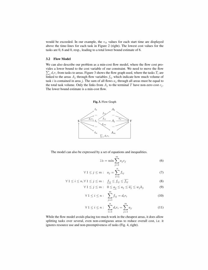
3.2 Flow Model

We can also describe our problem as a min-cost flow model, where the flow cost pro-vides a lower bound to the cost variable of our constraint. We need to move the flow∑i diri from tasks to areas. Figure 3 shows the flow graph used, where the tasks Ti are

linked to the areas Aj through flow variables fij which indicate how much volume oftask i is contained in area j. The sum of all flows aj through all areas must be equal tothe total task volume. Only the links from Aj to the terminal T have non-zero cost cj .The lower bound estimate is a min-cost flow.

Fig. 3. Flow Graph

S T

t1

...

ti

...

tn

A1

...

Aj

...

Am

diri aj

fi1

fij

fim

∑i diri

The model can also be expressed by a set of equations and inequalities.

lb = minm∑j=1

ajcj (6)

∀ 1 ≤ j ≤ m : aj =n∑i=1

fij (7)

∀ 1 ≤ i ≤ n, ∀ 1 ≤ j ≤ m : fij ≤ fij ≤ fij (8)

∀ 1 ≤ j ≤ m : 0 ≤ aj ≤ aj ≤ aj ≤ wjhj (9)

∀ 1 ≤ i ≤ n :m∑j=1

fij = diri (10)

∀ 1 ≤ i ≤ n :n∑i=1

diri =m∑j=1

aj (11)

While the flow model avoids placing too much work in the cheapest areas, it does allowsplitting tasks over several, even non-contiguous areas to reduce overall cost, i.e. itignores resource use and non-preemptiveness of tasks (Fig. 4, right).

The quality of the bound lb can be improved by computing tight upper bounds fij .Given a task i with domain d(si), we can compute the maximal overlap between thetask and the area j as:

fij = maxt∈d(si)

max(0, (min(xj + wj , t+ di)−max(xj , t))) ∗min(hj , ri) (12)

For the running example, the computed fij values are shown in Table 1 and the minimalcost flow is shown in Fig. 4. Its cost is 3 ∗ 0+3 ∗ 1+2 ∗ 2+1 ∗ 3 = 10. Note how bothtasks 1 and 2 are split into multiple pieces.

Fig. 4. Example Flow Bound

Flow Graph Assignment

S T

t1

t2

t3

A1

A2

A3

A4

A5

2

4

3

3

3

2

1

0

1

1

2

2

3

1

2

1

2

3

1

4

5

1

3

4

1

0

1

1

3

← j

← cj

← aj

lb = 1033 2 10

3.3 LP Models

The quality of the lower bound can be further improved by adding to the flow modelsome linear constraints, which limit how much of some task can be placed into low-cost areas. These models are no longer flows, but general LP models. We consider twovariations denoted as LP1 and LP2. We obtain LP1 by adding equations (13) to the LPformulation of the flow model (Constraints 6-11).

∀ 1 ≤ j ≤ m :n∑i=1

j∑k=1

fik =j∑

k=1

ak ≤ Bj =n∑i=1

bij (13)

The bij values tell us how much of task i can be placed into the combinationof cheaper areas {A1, A2, ...Aj}. Note that this is a stronger estimate, since bij ≤∑jk=1 fij . Therefore, the LP models dominate the flow model, but require a more ex-

pensive LP optimization at each step. Bj denotes the total amount of resources (fromall tasks) that is possible to place into the first j areas. We can compute the bij valueswith a sweep along the time axis.

Table 1. fij , bij and Bj Values for Example

fij 1 2 3 4 51 2 0 0 2 22 2 0 2 2 23 3 3 3 3 3

bij 1 2 3 4 51 2 2 2 2 22 2 2 2 4 43 3 3 3 3 3Bj 7 7 7 9 9

Table 1 shows the fij , bij and Bj values for the running example. The flow solutionin Fig. 4 does not satisfy equation (13) for j = 3, as a1 + a2 + a3 = 3 + 3 + 2 = 8 >b13 + b23 + b33 = 2+2+3 = 7. Solving the LP model finds an improved bound of 11.

The LP2 model produces potentially even stronger bounds by replacing constraints (13)with more detailed constraints on individual bij :

∀ 1 ≤ i ≤ n, ∀ 1 ≤ j ≤ m :j∑

k=1

fik ≤ bij (14)

In our example though, this model produces the same bound as model LP1.

4 Coarse Models and Greedy Algorithms

If we want to avoid running an LP solver inside our constraint propagator, we can deriveother lower bounds based on greedy algorithms.

4.1 Model A

We can compute a lower bound through a coarser model (denoted as Model A) whichhas m variables uj , denoting the total amount of work going into Aj .

lb = minm∑j=1

ujcj (15)

∀ 1 ≤ j ≤ m : uj ≤ wjhj (16)

∀ 1 ≤ j ≤ m : uj ≤n∑i=1

fij (17)

m∑j=1

uj =n∑i=1

diri (18)

It can be shown that this bound can be achieved by Algorithm A, which can bedescribed by the recursive equations:

lb =m∑j=1

ujcj (19)

∀ 1 ≤ j ≤ m : uj = min(n∑i=1

diri −j−1∑k=1

uk,

n∑i=1

fij , wjhj) (20)

The algorithm tries to fill the cheapest areas first as far as possible. For each areawe compute the minimum of the remaining unallocated task area, and the maximumamount that can be placed into the area based on the fij bounds and the overall areasize.

4.2 Model B

We can form a stronger model (Model B) by extending Model A with the constraints:

∀ 1 ≤ j ≤ m :j∑

k=1

uk ≤ Bj =n∑i=1

bij (21)

It can be shown that the lower-bound can be computed through Algorithm B, whichextends Algorithm A by also considering the Bj bounds (constraints (13)) and is recur-sively defined as:

lb =m∑j=1

ujcj (22)

∀ 1 ≤ j ≤ m : uj = min(n∑i=1

diri −j−1∑k=1

uk,

n∑i=1

fij , wjhj ,

n∑i=1

bij −j−1∑k=1

uk) (23)

Both algorithms A and B only compute a bound on the cost, and do not producea complete assignment of tasks to areas. On the other hand, they only require a singleiteration over the areas, provided the fij and bij bounds are known. Figure 5 comparesthe execution of algorithms A and B on the running example (top) and shows the re-sulting area utilization (bottom). Algorithm A computes a bound of 9, which is weakerthan the Flow Model (lb = 10). Algorithm B produces 11, the same as models LP1and LP2. Note that we can not easily determine which tasks are used to fill which area.

5 Direct Model

All previous models relied on a decomposition using a standard cumulative constraint toenforce overall resource limits. We now extend the model of the cumulative constraintgiven in [6] to handle the cost component directly (equations (24)-(33)).

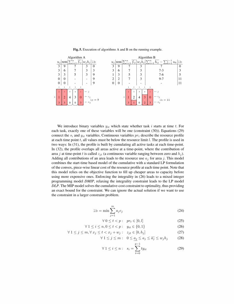
Fig. 5. Execution of algorithms A and B on the running example.

Algorithm A Algorithm Buj rem

∑ni=1 fij wjhj lb

3 9 7 3 03 6 7 3 33 3 5 3 90 0 - - 90 0 - - 9

uj rem∑n

i=1 fij wjhj

∑ni=1 bij −

∑j−1k=1 uk lb

3 9 7 3 7 03 6 7 3 7-3 31 3 5 3 7-6 52 2 7 3 9-7 110 0 - - - 11

1

2

1

2

3

1

4

5

1

3

4

1

0

1

1

3

← j

← cj

← aj

lp = 933 3 00

1

2

1

2

3

1

4

5

1

3

4

1

0

1

1

3

← j

← cj

← aj

lb = 1133 1 20

We introduce binary variables yit which state whether task i starts at time t. Foreach task, exactly one of these variables will be one (constraint (30)). Equations (29)connect the si and yit variables. Continuous variables prt describe the resource profileat each time point t, all values must be below the resource limit l. The profile is used intwo ways: In (31), the profile is built by cumulating all active tasks at each time-point.In (32), the profile overlaps all areas active at a time-point, where the contribution ofarea j at time-point t is called zjt (a continuous variable ranging between zero and hj).Adding all contributions of an area leads to the resource use aj for area j. This modelcombines the start-time based model of the cumulative with a standard LP formulationof the convex, piece-wise linear cost of the resource profile at each time point. Note thatthis model relies on the objective function to fill up cheaper areas to capacity beforeusing more expensive ones. Enforcing the integrality in (26) leads to a mixed integerprogramming model DMIP, relaxing the integrality constraint leads to the LP modelDLP. The MIP model solves the cumulative-cost constraint to optimality, thus providingan exact bound for the constraint. We can ignore the actual solution if we want to usethe constraint in a larger constraint problem.

lb = minm∑j=1

ajcj (24)

∀ 0 ≤ t < p : prt ∈ [0, l] (25)∀ 1 ≤ i ≤ n, 0 ≤ t < p : yit ∈ {0, 1} (26)

∀ 1 ≤ j ≤ m,∀ xj ≤ t < xj + wj : zjt ∈ [0, hj ] (27)∀ 1 ≤ j ≤ m : 0 ≤ aj ≤ aj ≤ aj ≤ wjhj (28)

∀ 1 ≤ i ≤ n : si =p−1∑t=0

tyit (29)

∀ 1 ≤ i ≤ n :p−1∑t=0

yit = 1 (30)

∀ 0 ≤ t < p : prt =∑

t′≤t<t′+di

yit′ri (31)

∀ 0 ≤ t < p : prt =m∑j=1

zjt (32)

∀ 1 ≤ j ≤ m : aj =xj+wj−1∑t=xj

zjt (33)

Example Figure 6 shows the solutions of DLP and DMIP on the running example.The linear model on the left uses fractional assignments for task 2, splitting it into twosegments. This leads to a bound of 12, while the DMIP model computes a bound of 15.

Fig. 6. Direct Model Example

Direct LP Direct MIP

1

2

1

2

3

1

4

5

1

3

4

1

0

1

1

3

← j

← cj

← aj

lb = 1233 1 11

1

2

1

2

3

1

4

5

1

3

4

1

0

1

1

3

← j

← cj

← aj

cost = 1523 2 02

6 Comparison

We now want to compare the relative strength of the different algorithms. We first definethe concept of strength in our context.

Definition 2. We call algorithm q stronger than algorithm p if its computed lowerbound lbq is always greater than or equal to lbp, and for some instances is strictlygreater than.

Theorem 1. The relative strength of the algorithms can be shown as a diagram, wherea line p → q indicates that algorithm q is stronger than algorithm p, and a dotted linebetween two algorithms states that they are incomparable.

Element

Alg A

Flow

Alg B

LP 1 LP 2 DLP DMIP

Proof. We need two lemmas, which are presented without proof:

Lemma 1. Every solution of the Flow Model is a solution of Model A.

Lemma 2. Every solution of the model LP1 is a solution of Model B.

This suffices to show that the Flow Model is stronger than Model A, and Model LP1is stronger than Model B. The other “stronger” relations are immediate. All “incompa-rable” results follow from experimental outcomes. Figure 7 shows as example wherethe Element Model and Algorithm A outperform the model DLP. Table 4 below showscases where the Element Model is stronger than Model A and Model LP2, and wherethe Flow Model outperforms Algorithm B.

Fig. 7. Example: Element and Flow Models stronger than DLP

lb(Element)=2 > lb(DLP)=0lb(Alg A)=2 > lb(DLP)=0

0 ← c1

4

1

1

1 ← c2

0 4

2

2

Why are so many of the models presented incomparable? They all provide differentrelaxations of the basic constraints which make up the CumulativeCost constraint.In Table 2 we compare our methods based on four main concepts, whether the algo-rithms respect the capacity limits for each single area, or for (some of the) multipleareas, whether the earliest start/latest end limits for the start times are respected, andwhether the tasks are placed as rectangles with the given width and height. Each methodrespects a different subset of the constraints. Methods are comparable if for all conceptsone model is stronger than the other, but incomparable if they relax different concepts.

Without space for a detailed complexity analysis, we just list on the right side ofTable 2 the main worst-case results for each method. We differentiate the time requiredto preprocess and generate the constraints, and the number of variables and constraintsfor the LP and MIP models. Recall that n is the number of tasks, m the number of areasand p the length of the scheduling period. Note that these numbers do not estimate thetime for computing the lower bounds but for setting-up the models.

7 Experiments

We implemented all algorithms discussed in the paper, referring to them as {DMIP,Element, Algo A, Algo B, Flow, LP1, LP2, DLP}. For convenience we denote them also

Table 2. Model Satisfies Basic Constraints/Complexity

MethodSingleArea

Capacity

MultiArea

Capacity

Earliest StartLatest End

TaskProfile

ModelSetup

Variables Constraints

Element no no yes yes O(npm) - -Flow yes no yes ≤ height O(nm) O(nm) O(n + m)

LP 1 yes Bj yes ≤ height O(nm2) O(nm) O(n + m)

LP 2 yes bij yes ≤ height O(nm2) O(nm) O(nm)Alg A yes no no no O(nm) - -Alg B yes Bj no no O(nm2) - -DLP yes yes yes width O(np + mp) O(n + m + p)

DMIP yes yes yes yes O(np + mp) O(n + m + p)

as Algo0, . . . , Algo7. We evaluated their performance over a number of instances, de-notedE. Each instance e ∈ E is defined by the areasA1, . . . , Am and tasks T1, . . . , Tn.In all experiments we use a day-long time horizon divided into 48 half-hour areas andtwo cost settings. In the first setting for each half-hour period we fix a price to givenvalues from a real-world price distribution (Fig. 1) over all the task specifications. Wedenote this as a fixed cost distribution (cost = fixed). Alternatively, for each area wechoose a random cost from interval [0, 100], for each task specification. We refer tothis as a random cost distribution (cost = random). In both cases the costs are nor-malized by subtracting the minimal cost cmin = minmj=1cj from each area cost. For agiven n, dmax, rmax, ∆ we generate tasks T1, . . . , Tn with randomly selected durationsdi ∈ [1, dmax] and resource consumptions ri ∈ [1, rmax], i = 1, . . . , n. ∆ denotes themaximal distance between the earliest and latest start time. For a given ∆ we randomlyselect the interval si ∈ [si, si] so that 0 ≤ si−si ≤ ∆. One of the major parameters weconsider is utilization defined as a portion of the total available area that must be coveredby the tasks: util =

∑ni=1 diri/(l · p). In the experiments we first decide the desired

level of utilization, util, and then select a corresponding capacity limit l = d∑n

i=1 diri

util·p e.Hence, each instance scenario is obtained by specifying (n, dmax, rmax, ∆, util, cost).

We used Choco v2.1.11 as the underlying constraint solver, and CPLEX v12.1 2 as aMIP/LP solver. The experiments ran as a single thread on a Dual Quad Core Xeon CPU,2.66GHz with 12MB of L2 cache per processor and 16GB of RAM overall, runningLinux 2.6.25 x64. All the reported times are in milliseconds.

General Comparison In the first set of experiments we compare the quality of thebounds for all algorithms presented. Let vali denote a value (lower bound) returned byAlgoi. The DMIP algorithm, Algo0 solves the problem exactly, yielding the value val0equal to the optimum. For other algorithms i we define its quality qi as vali/val0.

For a given instance we say that Algoi is optimal if qi = 100%. For all algorithmsexcept DMIP (i.e. i > 0), we say that they are the best if they have the maximal lower

1 http://choco-solver.net2 http://www-01.ibm.com/software/integration/optimization/cplex/

bound over the non-exact algorithms, i.e. qi = maxj>0qj . Note that the algorithmmight be best but not optimal. For a given scenario (n, dmax, rmax, ∆, util, cost) wegenerate 100 instances, and compute the following values: 1) number of times thatthe algorithm was optimal or best 2) average and minimal quality qi, 3) average andmaximal execution time. We evaluate the algorithms over scenarios with n = 100tasks, dmax = 8, rmax = 8, ∆ = 10, util ∈ {30%, 50%, 70%, 80%} and cost ∈{fixed, random}. This leads in total to eight instance scenarios presented in Table3. The first column indicates the scenario (utilization and cost distribution). The lasteight columns indicate the values described above for each algorithm. First note thatthe bound estimates for algorithms B, LP1, LP2 are on average consistently higher than95% over all scenarios, but that DLP provides exceptionally high bounds, on averageover 99.6% for each scenario. While algorithms A and Flow can provide weaker boundsfor lower utilization, the bounds improve for higher utilization. Algorithm Element onthe other hand performs better for lower utilization (since its bound ignores capacity l)and deteriorates with higher utilization.

Table 3. Evaluation of algorithms for dmax = rmax = 8 and∆ = 10 with varying util and cost.

Scenario Key DMIP Element A B Flow LP1 LP2 DLPutil=30 Opt/Best 100 - 92 92 0 0 0 0 0 0 0 0 0 0 93 100

fixed Avg/Min Quality 100.0 100.0 99.998 99.876 57.268 33.055 99.77 99.337 97.429 94.665 99.77 99.337 99.77 99.337 99.999 99.994Avg/Max Time 29 194 185 509 8 73 12 126 34 138 150 277 211 617 111 380

util=50 Opt/Best 100 - 2 2 0 0 0 0 0 0 0 0 0 0 7 100fixed Avg/Min Quality 100.0 100.0 99.038 94.641 68.789 54.22 99.131 95.963 97.816 95.89 99.407 97.773 99.435 97.913 99.948 99.358

Avg/Max Time 89 2,108 176 243 6 12 7 94 33 130 139 274 194 275 96 181util=70 Opt/Best 100 - 0 0 0 0 0 0 0 1 0 5 0 6 1 100

fixed Avg/Min Quality 100.0 100.0 93.541 81.603 84.572 69.953 96.495 87.884 99.1 96.994 99.24 97.838 99.346 98.071 99.764 98.992Avg/Max Time 2,107 32,666 177 242 7 103 8 72 34 97 136 239 213 1,798 110 1,551

util=80 Opt/Best 100 - 0 0 0 0 0 1 0 4 0 20 0 21 0 100fixed Avg/Min Quality 100.0 100.0 88.561 70.901 92.633 81.302 96.163 89.437 99.34 96.728 99.354 96.737 99.392 96.737 99.649 98.528

Avg/Max Time 13,017 246,762 206 450 10 67 15 96 38 124 156 235 220 426 125 299util=30 Opt/Best 100 - 94 94 0 0 0 0 0 0 0 0 0 0 97 100random Avg/Min Quality 100.0 100.0 99.996 99.872 58.094 41.953 96.965 93.237 73.759 54.641 96.965 93.237 96.966 93.254 99.999 99.977

Avg/Max Time 29 154 192 427 7 24 8 42 32 94 145 224 203 361 99 274util=50 Opt/Best 100 - 0 0 2 8 2 8 2 8 2 8 2 8 5 100random Avg/Min Quality 100.0 100.0 88.277 30.379 76.457 57.049 96.585 92.563 83.314 69.178 96.619 92.604 96.861 93.242 99.93 99.724

Avg/Max Time 2,452 62,168 202 814 10 99 13 131 43 177 165 380 238 903 108 327util=70 Opt/Best 100 - 0 0 0 0 0 0 0 0 0 0 0 0 0 100random Avg/Min Quality 100.0 100.0 91.045 72.06 89.784 75.822 95.242 90.496 92.953 84.277 95.953 92.24 96.947 94.012 99.697 99.374

Avg/Max Time 72,438 2,719,666 226 436 13 74 26 98 70 178 223 543 280 566 152 428util=80 Opt/Best 100 - 0 0 0 0 0 0 0 0 0 0 0 0 0 100random Avg/Min Quality 100.0 100.0 86.377 72.566 94.813 88.039 96.092 89.233 97.231 93.919 97.658 94.917 98.426 96.342 99.626 99.161

Avg/Max Time 684,660 8,121,775 320 2,148 16 100 31 180 63 370 223 1,586 363 23,91 286 7,242

We also performed experiments over unrestricted initial domains, i.e. where si ∈[0, p − 1]. While most of the algorithms improved their bound estimation, Elementperformed much worse for the fixed cost distribution, reaching quality as low as 12%for high utilization. On the other hand, reducing ∆ to 5 significantly improved thequality of Element, while slightly weakening the quality of other algorithms. In all thecases, the worst-case quality of DLP was still higher than 98.6%.

Aggregate Pairwise Comparison In Table 4 we compare all algorithms over the entireset of instances that were generated under varying scenarios involving 100 tasks. Forany two algorithms Algoi and Algoj let Eij = {e ∈ E | qei > qej} denote the set ofinstances where Algoi outperforms Algoj . Let numij = |Eij | denote the number ofsuch instances, while avgij and maxij denote the average and maximal difference inquality over Eij . In the (i, j)-th cell of Table 4 we show (numij , avgij ,maxij). In ap-proximately 2000 instances DLP strictly outperforms all other non-exact algorithms inmore than 1700 cases and is never outperformed by another. Algorithm B outperformsFlow (1107 cases) more often than Flow outperforming B (333 cases). Furthermore,LP2 outperforms LP1 in about 700 cases. Interestingly, even though Element produceson average weaker bounds, it is able to outperform all non-exact algorithms except DLPon some instances.

Table 4. Comparison of algorithms over all instances generated for experiments with n = 100 tasks.

Element A B Flow LP1 LP2 DLPDMIP 1802 26.39 88.62 1944 17.47 68.55 1944 3.99 30.71 1944 9.85 68.55 1944 3.49 30.71 1944 3.24 30.71 1387 0.18 1.47

EL - - - 1034 25.62 66.95 656 3.0 22.07 856 15.65 65.82 650 3.01 22.07 621 3.04 22.07A 1052 38.1 88.61 - - - - - - - - - - - - - - -B 1429 29.22 88.61 1439 18.22 66.65 - - - 1107 11.02 51.86 - - - - - -

FLW 1230 33.97 88.61 1184 12.51 64.35 333 2.39 10.49 - - - - - - - - -LP1 1436 29.74 88.61 1441 18.86 66.65 726 1.33 10.51 1413 8.75 51.86 - - - - - -LP2 1465 29.44 88.61 1441 19.19 66.65 846 1.71 10.64 1425 9.02 51.86 690 0.7 5.09 - - -DLP 1802 26.24 88.61 1752 19.24 68.55 1751 4.28 30.71 1747 10.82 68.55 1727 3.78 30.71 1725 3.51 30.71 - - -

Varying Number of Tasks Finally, we evaluated the effect of increasing the number oftasks. We considered scenarios n ∈ {50, 100, 200, 400} where dmax = 8, rmax = 8,∆ = 10, util = 70 and cost = random.The results are reported in Table 5. Wecan notice that all algorithms improve the quality of their bounds with an increase inthe number of tasks. While the time to compute the bounds grows for the non-exactalgorithms, interestingly this is not always the case for the DMIP model. The averagetime to compute the optimal value peaks for n = 100 (72 seconds on average) and thenreduces to 24 and 9 seconds for n = 200 and n = 400 respectively.

8 Conclusions and Future Work

We have introduced the CumulativeCost constraint, a resource cost-aware exten-sion of the standard cumulative constraint, and suggested a number of algorithms tocompute lower bounds on its cost. We compared the algorithms both theoretically andexperimentally and discovered that while most of the approaches are mutually incom-parable, the DLP model clearly dominates all other algorithms for the experiments con-sidered. Deriving lower bounds is a necessary first step towards the development ofthe CumulativeCost constraint. We plan to evaluate the performance of the con-straint in a number of real-life scheduling problems, which first requires developmentof domain filtering algorithms and specialized variable/value ordering heuristics.

Table 5. Evaluation of algorithms for random cost distribution,∆ = 10 and util = 70.

Scenario Key DMIP Element A B Flow LP1 LP2 DLPn=50 Opt/Best 100 0 0 0 0 0 0 0 0 0 0 0 0 0 0 100

Avg/Min Quality 100.0 100.0 89.331 71.865 88.833 70.372 93.991 86.143 92.384 84.589 94.863 87.417 95.899 89.937 98.664 95.523Avg/Max Time 1,334 31,426 102 314 8 83 6 36 23 78 93 254 132 298 75 233

n=100 Opt/Best 100 0 0 0 0 0 0 0 0 0 0 0 0 0 0 100Avg/Min Quality 100.0 100.0 91.045 72.06 89.784 75.822 95.242 90.496 92.953 84.277 95.953 92.24 96.947 94.012 99.697 99.374

Avg/Max Time 72,438 2,719,666 226 436 13 74 26 98 70 178 223 543 280 566 152 428n=200 Opt/Best 100 0 0 0 0 0 0 0 0 0 0 0 0 0 0 100

Avg/Min Quality 100.0 100.0 92.537 84.06 89.819 79.862 95.885 93.01 92.566 83.516 96.48 93.328 97.158 93.885 99.936 99.833Avg/Max Time 24,491 233,349 395 700 19 148 22 113 83 208 341 533 468 638 226 456

n=400 Opt/Best 100 0 0 0 0 0 0 0 0 0 0 0 0 0 0 100Avg/Min Quality 100.0 100.0 93.239 86.419 90.417 84.205 96.3 92.721 92.939 86.658 96.716 93.275 97.23 95.013 99.985 99.961

Avg/Max Time 9,379 158,564 831 1,222 31 164 36 189 181 305 923 3,053 1,214 3,434 484 871

References

1. A. Aggoun and N. Beldiceanu. Extending CHIP in order to solve complex scheduling prob-lems. Journal of Mathematical and Computer Modelling, 17(7):57–73, 1993.

2. P. Baptiste, C. Le Pape, and W. Nuijten. Constraint-Based Scheduling: Applying ConstraintProgramming to Scheduling Problems. Kluwer, Dortrecht, 2001.

3. Nicolas Beldiceanu and Mats Carlsson. A new multi-resource cumulatives constraint withnegative heights. In Pascal Van Hentenryck, editor, CP, volume 2470 of Lecture Notes inComputer Science, pages 63–79. Springer, 2002.

4. Nicolas Beldiceanu, Mats Carlsson, and Emmanuel Poder. New filtering for the cumulativeconstraint in the context of non-overlapping rectangles. In Laurent Perron and Michael A.Trick, editors, CPAIOR, volume 5015 of Lecture Notes in Computer Science, pages 21–35.Springer, 2008.

5. Nicolas Beldiceanu and Emmanuel Poder. A continuous multi-resources cumulative con-straint with positive-negative resource consumption-production. In Pascal Van Hentenryckand Laurence A. Wolsey, editors, CPAIOR, volume 4510 of Lecture Notes in Computer Sci-ence, pages 214–228. Springer, 2007.

6. John Hooker. Integrated Methods for Optimization. Springer, New York, 2007.7. Luc Mercier and Pascal Van Hentenryck. Edge finding for cumulative scheduling. INFORMS

Journal on Computing, 20(1):143–153, 2008.8. Andreas Schutt, Thibaut Feydy, Peter J. Stuckey, and Mark Wallace. Why cumulative de-

composition is not as bad as it sounds. In Ian P. Gent, editor, CP, volume 5732 of LectureNotes in Computer Science, pages 746–761. Springer, 2009.

9. Helmut Simonis and Trijntje Cornelissens. Modelling producer/consumer constraints. InUgo Montanari and Francesca Rossi, editors, CP, volume 976 of Lecture Notes in ComputerScience, pages 449–462. Springer, 1995.

10. Petr Vilı́m. Max energy filtering algorithm for discrete cumulative resources. In Willem Janvan Hoeve and John N. Hooker, editors, CPAIOR, volume 5547 of Lecture Notes in ComputerScience, pages 294–308. Springer, 2009.