Insurance: Mathematics and Economics 50 (2012) 12–25

Contents lists available at SciVerse ScienceDirect

Insurance: Mathematics and Economics

journal homepage: www.elsevier.com/locate/ime

Explaining young mortalityColin O’Hare ∗, Youwei LiSchool of Management, Queen’s University of Belfast, BT9 5EE, Belfast, United Kingdom

a r t i c l e i n f o

Article history:Received November 2010Received in revised formSeptember 2011Accepted 28 September 2011

JEL classification:C51C52C53G22G23J11

Keywords:MortalityStochastic modelsForecastingNon-linearity

a b s t r a c t

Stochastic modeling of mortality rates focuses on fitting linear models to logarithmically adjustedmortality data from the middle or late ages. Whilst this modeling enables insurers to project mortalityrates and hence pricemortality products it does not provide good fit for younger agedmortality. Mortalityrates below the early 20’s are important to model as they give an insight into estimates of the cohorteffect for more recent years of birth. It is also important given the cumulative nature of life expectancyto be able to forecast mortality improvements at all ages. When we attempt to fit existing models to awider age range, 5–89, rather than 20–89 or 50–89, their weaknesses are revealed as the results are notsatisfactory. The linear innovations in existing models are not flexible enough to capture the non-linearprofile of mortality rates that we see at the lower ages. In this paper, wemodify an existing 4 factor modelof mortality to enable better fitting to a wider age range, and using data from seven developed countriesour empirical results show that the proposed model has a better fit to the actual data, is robust, and hasgood forecasting ability.

© 2011 Elsevier B.V. All rights reserved.

1. Introduction

In recent years there has been an increasing amount of attentionput on the modeling of mortality risk as a significant risk thatpension providers and insurance firms are exposed to. Thesedevelopment have been driven in part by the introduction ofmore stringent regulation and historically low rates of interest andinflation. The later has exposed longevity risk as being a significantrisk in its own right and the development of innovative hedgingproducts has allowed risk holders to unbundle longevity risk fromthe interest and inflation risks.

There is a significant amount of literature on stochastic mod-eling of mortality rates. The impetus for the rapid development instochastic mortality modeling started with the often used modelof Lee and Carter (1992) who modeled US male data using a onefactor time series approach. Many innovations of the Lee–Cartermodel have been developed since including, Booth et al. (2002),Brouhns et al. (2002), Girosi and King (2005), Renshaw and Haber-man (2006), Cairns et al. (2006), Currie et al. (2004), Currie (2006),Hári et al. (2008), Tulijapurkar (2008) and Plat (2009).

Many papers propose that mortality in advanced ages isinfluenced by the mortality experiences at the younger age range

∗ Corresponding author. Tel.: +44 28 9097 4671; fax: +44 28 9097 4201.E-mail addresses: c.ohare@qub.ac.uk (C. O’Hare), y.li@qub.ac.uk (Y. Li).

0167-6687/$ – see front matter© 2011 Elsevier B.V. All rights reserved.doi:10.1016/j.insmatheco.2011.09.005

and it is clear that the average life expectancy of a populationwill be affected by experience at all ages. This cumulative effectmeans that experience at the younger ages is important to considerwhen modeling the mortality experience of a population. Froma demographic viewpoint, it is also clear that being able tomodel and forecast mortality at all ages is important. Hauserand Weir (2010) and Weir (2010) state that greater attentionmust be given to study designs that allow early-life exposures,experiences, and characteristics to be included in the analysisof outcomes in later life. Cohort effects1 have been identified asan important component in a mortality model and yet existingmodels are missing significant information on the most recentcohorts by excluding the younger ages from their models. Whenwe fit existing models to a wider age range starting from age 5rather than age 20 or 50, the results are not satisfactory2 sincethe linear innovations are not flexible enough to capture the non-linear dynamics at the lower ages, the so called ‘‘lifestyle’’mortality

1 The cohort effect was identified in reports by the Government Actuary’sDepartment (1995, 2001, 2002). These reports highlighted that the generationsborn between 1925 and 1945 (centered on the generation born in 1931)experienced more rapid improvement than earlier and later generations. Thisfeature had been noted for both males and females in the UK.2 We show later in the paper that fitting errors more than double in some cases

when a wider age range is fitted. See Tables 6 and 7 model M9 for example.

C. O’Hare, Y. Li / Insurance: Mathematics and Economics 50 (2012) 12–25 13

(accidents, drug abuse) profile. In this paperwepropose amortalitymodel that aims to improve upon the fit quality of existing modelson a wider age range whilst at the same time not losing sight ofthe positive aspects of existing models. In particular, using a widerage range introduces a non-linear profile of mortality and we aimto capture this in a better way.

Using the data of a range of developed countries’ from 1950–2006 we find that the proposed model fits the data very well, isapplicable to a fuller age range and captures the cohort effect. Italso has a non-trivial correlation structure, captures the non-lineareffects at lower ages, has no robustness problems and can take intoaccount parameter risk, while the structure of the model remainsrelatively simple.

The remainder of the paper is organized as follows. First, inSection 2 the background to stochastic mortality modeling isreviewed. In Section 3 an empirical comparison of existing modelsis conducted which further motivates the paper. In Section 4 amodification of the Plat (2009) model is proposed and its fittingand forecasting performance is assessed using the mortality dataof 7 different countries. Conclusions are drawn in Section 5.

2. Background

Due to the increasing focus on risk management and measure-ment for insurers and pension funds, the literature on stochas-tic mortality models has developed rapidly during the last twentyyears. A need to measure the performance quality of these modelsled to the development of a range of criteria against which mod-els could be assessed. In this section we discuss the background tostochastic mortality modeling starting with the criteria. We followthis with an overview of existing stochastic mortality models up toand including the Plat (2009) model.

In order to assess the quality of a model (from both a fitting anda forecasting perspective) we need to have a range of metrics onwhichwe can quantify the performance of themodel. A good set ofcriteria should allow us to quantify the performance of a mortalitymodel against a range of aspects considered to be ‘‘good qualities’’for a model of mortality rates. Cairns et al. (2011) proposed criteriaagainst which a model can be assessed. For example, the modelmust fit the existing datawell, themodelmust produce biologicallyreasonable forecasts etc. Using these criteria we can determinehow good a particular model is at fitting and forecasting mortality.

Stochastic mortality models either model the central mortalityrate or the initial mortality rate (see Coughlan et al., 2007). Let Dx,tbe the number of people with age x that died in year t , and Ex,t , theexposure being the average population with age x in the year t , thecentral mortality rate3 mx,t is defined as:

mx,t =Dx,t

Ex,t. (1)

The first and most well known stochastic mortality model isthat of Lee and Carter (1992):ln(mx,t) = ax + bxκt + ϵx,t , (2)where ax and bx are age effects and κt is a random period effect.4Applying the necessary constraints the ax are given by

ax =1N

Nt=1

lnmx,t . (3)

The bilinear part bxκt was then determined as the first singularcomponent of a singular value decomposition (SVD), with the

3 The initial mortality rate qx is the probability that a person aged x dies withinthe next year. The different mortality measures are linked by the approximation:qx ≈ 1 − e−mx .4 This model was fitted to US mortality data for ages 0–110 between the years of

1933 and 1987.

remaining information from the SVD considered to be part of theerror structure. The κt are estimated and refitted to ensure themodel maps onto historic data and the subsequent time seriesκt is used to forecast mortality rates using normal time seriesforecasting techniques.

Among many discussions of the Lee–Carter model, Cairnset al. (2006, 2009, 2011) summarized the main disadvantagesof the model. The model has one factor, resulting in mortalityimprovements at all ages being perfectly correlated (trivialcorrelation structure). For countries where a cohort effect isobserved in the past, the model gives a poor fit to historicaldata. The uncertainty in future death rates is proportional to theaverage improvement rate bx which for high ages can lead to thisuncertainty being too low, since historical improvement rates haveoften been lower at high ages. Also, the model can result in a lackof smoothness in the estimated age effect bx.

Despite the weaknesses of the Lee–Carter model its simplicityhas led to it being taken as a benchmark against which otherstochastic mortality models can be assessed. There has beena significant amount of literature developing additions to, ormodifications of, the Lee–Carter model. For example Booth et al.(2002), Brouhns et al. (2002), Lee and Miller (2001), Girosi andKing (2005), De Jong and Tickle (2006), Delwarde et al. (2007) andRenshaw and Haberman (2003, 2006).

Mortality data is 2 dimensional with deaths and exposuresbeing recorded by year and by age. We can therefore considerthe data from three different viewpoints, the age profile (or howmortality changes from age to age), the time profile (howmortalityrates for a specific age change over time), and more recentlyidentified, the cohort profile (how mortality for a specific cohortof the population – those born in a particular year – changes inrelation to other cohorts). The Lee–Carter model identified theinteraction between age and time through the one bilinear factorbxκt . Many of the modifications since the Lee–Carter model havesought to capture additional age–period effects or cohort effectsand they can be grouped as such.

2.1. Cohort effect additions

Renshaw and Haberman (2006) modified the Lee–Carter modelby simply adding a factor γt−x to capture effects that could beattributed to the year of birth (t − x),

ln(mx,t) = ax + b1xκt + b2xγt−x + ϵx,t , (4)where κt is defined as before and γt−x is a random cohort effect.

The model does have a much better fit for countries such as theUK where a cohort effect has been identified, however it suffersfrom a lack of robustness perhaps due to the presence of morethan one local maximum in the likelihood function. Among others,for instance Currie (2006) noted that if the model was fitted usingdata from 1961–2000 then the parameters showed qualitativelydifferent characteristics to those obtained when fitting to datafrom1981–2000. Furthermore, as noted by Currie (2006), althoughthemodel incorporates the cohort effect, for most of the simulatedmortality rates the correlation structure is still trivial with thesimulated cohort parameters only being relevant for the higherages at the far end of the projection.

Following this analysis Currie (2006) applied a simplified age–period–cohort model of Clayton and Schifflers (1987) to mortalitywhich removed the robustness problem but at the expense of thefitting quality:ln(mx,t) = ax + κt + γt−x + ϵx,t . (5)

2.2. Age–period effect additions

Cairns et al. (2006) observed that for England and Wales andUnited States data, the fitted cohort effect appeared to have a

14 C. O’Hare, Y. Li / Insurance: Mathematics and Economics 50 (2012) 12–25

trend in the year of birth. This suggested that the cohort effect wascompensating for the lack of a second age–period effect, as wellas trying to capture the cohort effect in the data. This led them tointroduce a two factor model of mortality,

logit(qx,t) = κ1t + κ2

t (x − x̄) + ϵx,t , (6)

where x̄ is the mean age in the sample range and (κ1t , κ

2t ) are

assumed to be a bivariate random walk with drift. The two factorsin this model were both period factors with no cohort effectallowed for. This was rectified in Cairns et al. (2009), namelycapturing the cohort effect as an additional effect on top of the twoage–period effects. All thesemodels havemultiple factors resultingin a non-trivial correlation structure which mirrors the realitythat improvements in mortality rates are different for differentage ranges. A further adaptation was also created allowing for thecohort effect to diminish over time. The main problem with thesemodels arises from the fact that they were designed for higherages and so ignored the modeling of mortality at the lower ages(for example the accident hump). Cairns et al. (2009) argue thatthe significant cost associated with mortality is at the older agesand thus their modeling focused on those ages. When using thesemodels for full age ranges, the fit quality is relatively poor and theprojections are biologically unreasonable.

2.3. Age–period and cohort additions combined

Plat (2009) wanted to develop a model which maintainedthe good aspects of the existing models whilst leaving out theweaker features. The result was a four factor model which took itsbeginnings from the Lee–Carter model and which added factors tocapture the second age–period effect, as per the Cairns et al. (2006)model and the cohort effect, as per the Renshaw and Haberman(2006) model. The innovation in the Plat model was to then add afurther period factor affecting only the lower ages and designedto allow the model to fit to the whole age range. The modelspecification is given by:

ln(mx,t) = ax + κ1t + κ2

t (x̄ − x) + κ3t (x̄ − x)+ + γt−x + ϵx,t , (7)

where the ax is similar to that of the Lee–Carter model andmakes sure that the overall shape of the mortality curve by ageis reasonable, the κ1

t and κ2t model the mortality rates as in the

Cairns et al. (2006) model and the κ3t models the effects specific to

the lower ages onlywhere (x̄−x)+ takes the value (x̄−x)when thisis positive and zero otherwise. Finally the γt−x models the cohorteffect.

The range of existing models described above meet most of thecriteria set out by Cairns et al. (2011) and the Plat model meetsall of the criteria by its very design. However, when the age rangeis widened to allow for the non-linear characteristics of youngmortality experience then as far as we are aware, none of theexistingmodelsmeet the above criteria adequately (although someare close). This is the starting point of this paper.

3. Empirical comparison of existing models

In this section we empirically compare the existing models tosee their performance when the age range is widened to allowfor the non-linear mortality experience at lower ages. For ease ofnotation we will use the naming convention established by Cairnset al. (2009). Table 5 in the Appendix sets out the names we willuse for each of the models.

We fit the models to different countries and to different ageranges for each country. The data sets5 used are: Male mortality

5 The data consists of numbers of deaths Dx,t and the corresponding exposuresEx,t and is extracted from: www.mortality.org, see HMD (2004).

Table 1The MAPE for the model fit to ages 5–89 (%).

Model M1 M2 M3 M5 M6 M7 M9

GB 6.14 3.91 6.96 21.83 16.71 12.88 7.56E&W 6.38 4.16 7.08 21.83 16.87 13.03 7.64SCO 10.97 9.28 12.76 19.99 18.74 15.76 14.72US 4.58 2.96 5.43 16.08 15.59 15.20 5.65NL 8.99 7.01 7.91 23.57 17.82 12.95 7.22AUS 7.45 6.44 8.80 23.86 20.46 18.52 9.61NZ 12.32 11.86 13.66 27.42 25.46 23.84 13.74

Table 2The MAPE for the model fit to ages 20–89 (%).

Model M1 M2 M3 M5 M6 M7 M9

GB 14.45 3.19 14.53 16.53 9.93 7.60 3.27E&W 14.34 3.39 14.42 16.82 10.09 7.73 3.50SCO 15.67 6.31 15.70 16.45 10.32 8.81 6.31US 12.47 2.46 12.53 14.07 7.92 6.30 2.76NL 12.54 4.16 12.62 16.14 11.20 8.03 4.22AUS 5.67 4.56 5.84 17.10 10.99 8.40 5.25NZ 9.57 8.57 9.26 19.20 15.32 12.06 9.19

Table 3The MAPE for the model fit to ages 50–89 (%).

Model M1 M2 M3 M5 M6 M7 M9

GB 2.86 1.75 2.00 3.87 1.93 1.53 1.36E&W 2.94 1.87 2.13 4.03 2.02 1.62 1.48SCO 4.05 3.33 3.17 4.57 3.29 3.14 2.82US 2.21 1.47 1.61 2.52 2.09 1.87 1.41NL 4.05 2.39 2.59 4.01 2.19 2.16 2.07AUS 3.18 3.22 3.78 3.62 2.94 2.65 2.59NZ 5.64 5.46 5.94 6.35 5.81 5.78 5.37

data during 1950–2006 for age ranges 5–89, 20–89 and 50–89of Great Britain (GB), England and Wales (E&W), Scotland (SCO),United States (US), Australia (AUS), New Zealand (NZ), and TheNetherlands (NL). Although a longer history is available for someof the countries, we have used the period 1950–2006 for all thecountries as this data is more reliable and will allow a validcomparison with the results of Cairns et al. (2009, 2011), andwith Plat (2009) who used the period 1960–2006. The model fitis compared using the Mean Average Percentage Error (MAPE)measure and the Bayesian Information Criterion(BIC) measure.

The MAPE measures the average difference in absolute valuebetween m̂x,t , the estimate ofmx,t , and mx,t itself, it is defined by:

MAPE =1

NM

x,t

∥m̂x,t − mx,t∥

mx,t(8)

where we have N time dimensions (in this case N = 57) and Mage dimensions (in this caseM = 70). The BIC measure provides atrade-off between fit quality and parsimony of the model and it isdefined as:

BIC = L(φ̂) −12K ln(P), (9)

where L(φ̂) is the log-likelihood of the estimated parameter φ̂, Pis the number of observations and K is the number of parametersbeing estimated.

Table 1 gives a comparison of the fitting results (in terms ofMAPE) to the age range 5–89. Tables 2 and 3 show the fitting resultsto ages 20–89 and 50–89. We see from Tables 1 and 2 that when awide age range is used (5–89 or 20–89), the Plat model M9 is notthe best fitting model, however, if we exclude model M2, whichsuffers from robustness issues, the Plat model is confirmed to bethe best fitting model over the age range 20–89. When fitting tothe age ranges 5–89 and 20–89 it is important to note that the

C. O’Hare, Y. Li / Insurance: Mathematics and Economics 50 (2012) 12–25 15

1950 1960 1970 1980 1990 2000 2010 1950 1960 1970 1980 1990 2000 2010–7

–6.8

–6.6

–6.4

–6.2

–6

1950 1960 1970 1980 1990 2000 2010–5.2

–5

–4.8

–4.6

–4.4

–4.2

1950 1960 1970 1980 1990 2000 2010–3.2

–3

–2.8

–2.6

–2.4

–2.2

–8.5

–8

–7.5

–7a b

c d

Fig. 1. Logarithm of mortality by year for GB males aged (a) 15, (b) 35, (c) 55, and (d) 75.

1950 1960 1970 1980 1990 2000 2010–7.8

–7.6

–7.4

–7.2

–7

–6.8

–6.6

–6.4

1950 1960 1970 1980 1990 2000 2010–6.6

–6.5

–6.4

–6.3

–6.2

–6.1

–6

–5.9

–5.8

1950 1960 1970 1980 1990 2000 2010–5

–4.8

–4.6

–4.4

–4.2

–4

1950 1960 1970 1980 1990 2000 2010–3.2

–3.1

–3

–2.9

–2.8

–2.7

–2.6

–2.5

–2.4

a b

c d

Fig. 2. Logarithm of mortality by year for US males aged (a) 15, (b) 35, (c) 55, and (d) 75.

models of Cairns et al. (2006, 2009) do not perform very well forthese age ranges, since theywere designed for higher ages only. Forcomparison we also fit the existing models to data between 1950and 2006 for ages 50–89 only. Table 3 shows that the Plat modelstill outperforms other models.

We also look at the fitting results based on the BIC. Tables 6–8 in the Appendix show the BIC measures for the seven countries,based on fitting to the full age 5–89, the 20–89 age range, and the50–89 age range, respectively. We see from the tables that it isunclear which model is the best performing using a BIC measurewith the Renshaw–Haberman model, M2, showing some goodfitting performances, but with models M3, M5, M6, and M9, allperforming well on some countries data sets. A particular point tonote at this stage (and to motivate the discussion further), is thatby widening the age range from 20–89 to 5–89 we can see that forthe Platmodel for example, the fit qualitymoves from 3.27% on the20–89 age range to 7.56% on the 5–89 age range.

Table 4MAPE and BIC results for model M10.

Country MAPE BIC5–89 20–89 50–89 5–89 20–89 50–89

GB 5.88 2.77 1.29 −28326 −21887 −13148E&W 6.05 2.79 1.37 −27549 −21634 −13074SCO 11.88 2.79 2.76 −18586 −15768 −10096US 4.14 2.31 1.35 −50487 −29998 −18727NL 6.11 2.67 1.99 −19586 −16729 −10601AUS 8.14 2.65 2.48 −22466 −18327 −10956NZ 13.65 2.69 5.39 −17272 −14714 −9433

To understand why the Plat model does not perform very wellfor the wider age range and to motivate our further analysis, welook at male data from GB and US. At first, it might be informativeto split the data into the period effect and the age effect. Figs. 1and 2 plot the time effect for GB and US males at ages 15, 35, 55

16 C. O’Hare, Y. Li / Insurance: Mathematics and Economics 50 (2012) 12–25

5 25 45 65 85 105–8

–7

–6

–5

–4

–3

–2

–1

5 25 45 65 85 105–8

–7

–6

–5

–4

–3

–2

–1

5 25 45 65 85 105–10

–8

–6

–4

–2

0

5 25 45 65 85 105–10

–8

–6

–4

–2

0

a b

c d

Fig. 3. Logarithm of mortality for GB males during the years (a) 1950, (b) 1965, (c) 1980, and (d) 2005.

–8

–7

–6

–5

–4

–3

–2

–1

–8

–7

–6

–5

–4

–3

–2

–1

–10

–8

–6

–4

–2

0

–10

–8

–6

–4

–2

0

5 25 45 65 85 105 5 25 45 65 85 105

5 25 45 65 85 105 5 25 45 65 85 105

a b

c d

Fig. 4. Logarithm of mortality for US males during the years (a) 1950, (b) 1965, (c) 1980, and (d) 2005.

and 75with each graph showing the natural logarithm ofmortalitybetween the years 1950 and 2006. We see from Figs. 1 and 2 thatthe logarithm of mortality for both GB and US shows a markedlydownward trend over time for each of the age ranges, and themortality looks more volatile at the younger ages, in this casethe 15 and 35 year old samples. This might be attributed to thesmall numbers of deaths at those ages and the fact that deaths atthe lower ages are due to a wider range of causes influenced by‘‘lifestyle’’ choices and so are not linked to general deteriorationdue to ill health and old age.

Focusing on specific years and looking at the mortality effectfor the whole age range, in Figs. 3 and 4, we can see that a linearpattern does emerges beyond age 25 or so, however, looking at themortality below that age we see a very clear non-linear patternarising. Again this is due to ‘‘lifestyle’’ factors and in order tomodelthese effects we require more flexibility in the factors than theexisting model allow.

Looking at the 4 factor model of Eq. (7), the design innovationwas to include the additional factor κ3

t (x̄− x)+. This factor adds, ina linear way, an additional flexibility for ages less than themean ofthe data set. In the case of Plat this would be for ages less than 55.Figs. 3 and 4 show clearly that the logarithm of mortality for agesbelow the mean of 55 are far from linear.

Aswehave seen fromTables 1–3whilst the Platmodel performsrelativelywell when fit to the data set from age 20, its performancedips somewhat when fitted to the larger data set. In terms of theMAPE when looking at Tables 1 and 2 we find that when the widerage range is fitted the percentage error more than doubles acrossall countries for which we have fit the model. This implies thatthe addition of a fourth linear factor is inadequate when modelingmortality at lower ages. In the following section we propose amodification to the Plat model which introduces some additionalflexibility into the model allowing it to be more adequately fittedto a wider age range.

C. O’Hare, Y. Li / Insurance: Mathematics and Economics 50 (2012) 12–25 17

1950 1960 1970 1980 1990 2000 2010–0.4

–0.2

0

0.2

0.4

0.6

1950 1960 1970 1980 1990 2000 2010–14

–12

–10

–8

–6

–4

–2x 10–3

1950 1960 1970 1980 1990 2000 2010–0.015

–0.01

–0.005

0

0.005

0.01

0.015

1860 1880 1900 1920 1940 1960–0.2

–0.1

0

0.1

0.2

a b

c d

Fig. 5. Estimated values of (a) κ1t , (b) κ2

t , (c) κ3t , and (d) γt−x based on GB males aged 5–89 between years 1950 and 2006.

Table 5The names of stochastic mortality models.

Name Model and name

M1 Lee and Carter (1992)ln(mx,t ) = ax + bxκt + ϵx,t

M2 Renshaw and Haberman (2006)ln(mx,t ) = ax + b1xκt + b2xγt−x + ϵx,t

M3 Currie (2006)ln(mx,t ) = ax + κt + γt−x + ϵx,t

M5 Cairns et al. (2006)logit(qx,t ) = κ1

t + κ2t (x − x̄) + ϵx,t

M6 Cairns et al. (2009) with cohort effectlogit(qx,t ) = κ1

t + κ2t (x − x̄) + γt−x + ϵx,t

M7 Cairns et al. (2009) with cohort and quadratic age effectlogit(qx,t ) = κ1

t + κ2t (x − x̄) + κ3

t ((x − x̄)2 − σ 2x ) + γt−x + ϵx,t

M9 Plat (2009)ln(mx,t ) = ax + κ1

t + κ2t (x̄ − x) + κ3

t (x̄ − x)+ + γt−x + ϵx,tM10 Quadratic effect model

ln(mx,t ) = ax+κ1t +κ2

t (x̄−x)+κ3t

(x̄−x)++[(x̄−x)+]

2+γt−x+ϵx,t

Note: The model M4 and M8 are not included in our analysis. The M4 is a P-splinesmodel developed in Currie (2006), it is of a structurally different nature to theremaining stochasticmodels. TheM8 in Cairns et al. (2009)with diminishing cohorteffect is a modification of theM5, it was primarily designed for ages over and above50. The M10 is the model that we propose in this paper.

4. A modification to the Plat model

In this section we incorporate the non-linear features ofmortality at younger ages into an adaptation of the Plat modelproposing an alternative better fitting model. We show the qualityof the fit of the proposed model with that of the existing modelsby fitting to data from a range of countries for the age ranges 5–89,20–89 and 50–89 and for years 1950–2006.

4.1. The model

Wemodel the central mortality ratemx,t as:

ln(mx,t) = ax + κ1t + κ2

t (x̄ − x) + κ3t

(x̄ − x)+ + [(x̄ − x)+]

2+ γt−x + ϵx,t , (10)

where ax makes sure that the basic shape of the mortality curveover ages is in linewith historical observations as in the Lee–Cartermodel (2) and the κ1

t factor represents changes in the level of

0 10 20 30 40 50 60 70 80 90–9

–8

–7

–6

–5

–4

–3

–2

Fig. 6. Estimated values of ax based on GB males aged 5–89 between years 1950and 2006.

mortality for all ages. Following the reasoning in Cairns et al.(2006), the (long-term) stochastic process for this factor shouldnot be mean reverting. The κ2

t factor allows changes in mortalityto vary between ages reflecting the historical observation thatimprovement rates can differ for different age classes and κ3

tmodels the effects specific to the lower age only as in the Platmodel(7). The adjusted coefficient ofκ3

t is designed to capture someof thenon-linear effects observed at the lower ages, the ‘‘quadratic lowerage effect’’.6 Finally the γt−x models the cohort effect in the sameway as the models of Currie (2006), Cairns et al. (2009) and Plat(2009). The proposed model (10) has 4 stochastic factors, and sohas a relatively simple structure similar to the Plat (2009), Currie(2006) and the Cairns et al. (2006) models.

Historical data indicates that the dynamics of mortality ratesat lower ages (up to age 40/50) whilst still showing a downwardtrend over time does showmuchmore variation around the trend.This can be attributed in part to the small number of deaths

6 We also look at themore general case ln(mx,t ) = ax +κ1t +κ2

t (x̄−x)+κ3t

(x̄−

x)+ + a[(x̄ − x)+]2

+ γt−x + ϵx,t where the parameter ‘‘a’’ was included to test arange of different quadratic coefficients. However, we found that the fit quality didnot vary much, on both BIC and MAPE for non-zero values of ‘‘a’’, and we thereforefocus on a model with a parameter a = 1. Results of general ‘‘a’’ are available onrequest.

18 C. O’Hare, Y. Li / Insurance: Mathematics and Economics 50 (2012) 12–25

1950 1960 1970 1980 1990 2000 2010–0.6

–0.4

–0.2

0

0.2

1950 1960 1970 1980 1990 2000 2010–2

0

2

4

6

8x 10

–3

1950 1960 1970 1980 1990 2000 2010 1860 1880 1900 1920 1940 1960–0.2

–0.1

0

0.1

0.2

a b

c d

–0.01

–0.005

0

0.005

0.01

Fig. 7. Estimated values of (a) κ1t , (b) κ2

t , (c) κ3t , and (d) γt−x based on US males aged 5–89 between years 1950 and 2006.

0 10 20 30 40 50 60 70 80 90–8

–7

–6

–5

–4

–3

–2

Fig. 8. Estimated values of ax based on US males aged 5–89 between years 1950and 2006.

and in part to the nature of deaths at these ages, the so called‘‘lifestyle’’ mortality factors (smoking, drug abuse, alcohol abuse,car accidents and violence) for example. In the Platmodel the factorκ3t was added. In model (10) we modify the coefficient of κ3

t tocapture the non-linear dynamics observed in the historical data.

The factor κ1t shows a trend and is fitted with a non-stationary

ARIMA process. The factors κ2t and κ3

t allow the model tohave a non-trivial correlation structure between ages. Fitting anon-stationary ARIMA-process for these factors could result (insome scenarios) in projected scenarios where the shape of themortality curve over ages is not biologically reasonable. Therefore,a stationary (mean reverting) process will be assumed for thesefactors. The process for the cohort effect factor γt−x should nothave a trend since we should not expect cohort effects to improveyear on year. Therefore, a trendless mean reverting process will beassumed for γt−x.

As with all stochastic mortality models, the mortality modelproposed above has an identifiability problem, meaning thatdifferent parameterizations could lead to identical values forln(mx,t). However, this can be resolved by setting identifiabilityconstraints. As the model has the same time series structure tothat of the Plat (2009), following an approach of Cairns et al. (2009,model M6), we have

(1)c=cl

c=c0γc = 0

(2)c=cl

c=c0cγc = 0

(3)

t κ3t = 0

where c0 and c1 are the earliest and latest year of birth to which acohort effect is fitted, and c = t−x. These constraints are the sameas for the Plat (2009) model as is the rationale behind the choice ofthe constraints.

Fitting methodology—The original method by which to fit such astochastic model was to use SVD as used in Lee and Carter (1992).Brouhns et al. (2002) described an alternative fitting methodologyfor the Lee–Carter model in which the number of deaths Dx,t ismodeled as a Poisson distribution with parameter (Ex,tmx,t)wheremx,t is the mortality rate we are estimating. The main advantageof the Brouhns et al. (2002) approach over the SVD approach isthat it accounts for the heteroscedasticity of the mortality data fordifferent ages. Indeed this method has been usedmore commonly,see for example Renshaw and Haberman (2003, 2006), Cairns et al.(2009) and Plat (2009). We adopt this approach and model thenumber of deaths by Dx,t ≈ Poisson(Ex,tmx,t). The parametersof model (10) are estimated by maximizing the log-likelihoodfunction7:

L(φ;D, E) =

x,t

Dx,t ln[Ex,tmx,t(φ)]

− Ex,tmx,t(φ) − ln(Dx,t !). (11)

Besides estimates for ax, the fitting procedure described aboveleads to time series of estimations of κ1

t , κ2t , κ

3t , and γt−x. After

fitting the model we take the fitted values for the time series andfit suitable ARIMA-processes.

4.2. Comparison of fit quality with existing models

To evaluate whether the proposed model fits historical datawell, we fit the model to the data sets described in Section 3. We

7 We used an adaptation of the R-code of the software package ‘‘Lifemetrics’’which is an open source toolkit for measuring and managing longevity andmortality risk, designed by J.P. Morgan, see http://www.lifemetrics.com andhttp://www.r-project.org/.

C. O’Hare, Y. Li / Insurance: Mathematics and Economics 50 (2012) 12–25 19

1950 1970 1990 2010 203010

10

10–3

10–3

–4

10–2

10–1

–5

1950 1970 1990 2010 2030

1950 1970 1990 2010 2030 1950 1970 1990 2010 2030

a b

c d

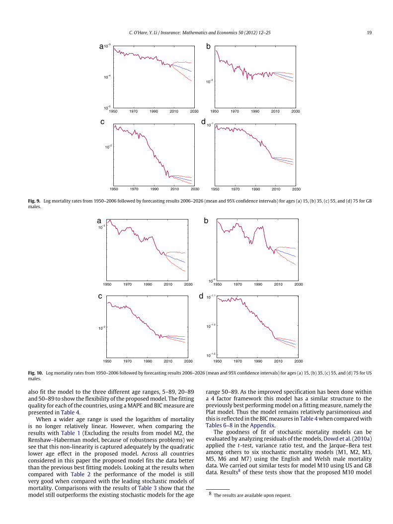
Fig. 9. Log mortality rates from 1950–2006 followed by forecasting results 2006–2026 (mean and 95% confidence intervals) for ages (a) 15, (b) 35, (c) 55, and (d) 75 for GBmales.

10–3

10–3

10–2

1950 1970 1990 2010 2030 1950 1970 1990 2010 2030

1950 1970 1990 2010 2030 1950 1970 1990 2010 2030

10–1.5

10–1.3

10–1.1

a b

c d

Fig. 10. Log mortality rates from 1950–2006 followed by forecasting results 2006–2026 (mean and 95% confidence intervals) for ages (a) 15, (b) 35, (c) 55, and (d) 75 for USmales.

also fit the model to the three different age ranges, 5–89, 20–89and 50–89 to show the flexibility of the proposedmodel. The fittingquality for each of the countries, using aMAPE and BICmeasure arepresented in Table 4.

When a wider age range is used the logarithm of mortalityis no longer relatively linear. However, when comparing theresults with Table 1 (Excluding the results from model M2, theRenshaw–Haberman model, because of robustness problems) wesee that this non-linearity is captured adequately by the quadraticlower age effect in the proposed model. Across all countriesconsidered in this paper the proposed model fits the data betterthan the previous best fitting models. Looking at the results whencompared with Table 2 the performance of the model is stillvery good when compared with the leading stochastic models ofmortality. Comparisons with the results of Table 3 show that themodel still outperforms the existing stochastic models for the age

range 50–89. As the improved specification has been done withina 4 factor framework this model has a similar structure to thepreviously best performingmodel on a fittingmeasure, namely thePlat model. Thus the model remains relatively parsimonious andthis is reflected in the BICmeasures in Table 4when comparedwithTables 6–8 in the Appendix.

The goodness of fit of stochastic mortality models can beevaluated by analyzing residuals of themodels, Dowd et al. (2010a)applied the t-test, variance ratio test, and the Jarque–Bera testamong others to six stochastic mortality models (M1, M2, M3,M5, M6 and M7) using the English and Welsh male mortalitydata. We carried out similar tests for model M10 using US and GBdata. Results8 of these tests show that the proposed M10 model

8 The results are available upon request.

20 C. O’Hare, Y. Li / Insurance: Mathematics and Economics 50 (2012) 12–25

a b

c d

1950 1960 1970 1980 1990 2000 20100

0.2

0.4

0.6

0.8

1950 1960 1970 1980 1990 2000 2010–0.022

–0.02

–0.018

–0.016

–0.014

–0.012

–0.01

1950 1960 1970 1980 1990 2000 2010–4

–2

0

2

4

6x 10

–4

1860 1880 1900 1920 1940 1960–0.2

–0.1

0

0.1

0.2

Fig. 11. Estimated values of (a) κ1t , (b) κ2

t , (c) κ3t , and (d) γt−x based on GB males aged 5–89 between years 1950 and 2006 for the Plat model.

–9

–8

–7

–6

–5

–4

–3

–2

–1

0 10 20 30 40 50 60 70 80 90

Fig. 12. Estimated values of ax based on GB males aged 5–89 between years 1950and 2006 for the Plat model.

performs adequately when compared to those in the Dowd et al.(2010a).

Fitting the ARIMA processes—In the remainder of this subsection,we focus on the populations of GB and US males and on fitting tothe age range 5–89. After fitting the model to the population datathe next step is to select and fit suitable ARIMA-process to the timeseries’ of κ1

t , κ2t , κ

3t , and γt−x. The fitted parameters κ1

t , κ2t , κ

3t , and

γt−x for GB males are given in Fig. 5 and for US males are given inFig. 7. The estimates for theαx parameters are given in Figs. 6 and 8.The figures shows that the pattern of the important parameter κ1

t iswell-behaved. The patterns of the other parameters all reveal someautoregressive behavior. Since the factor κ1

t drives a significantpart of the uncertainty in mortality rates, its relatively regularbehavior (for this particular dataset)will also show in the relativelynarrow confidence intervals.

a b

c d

1950 1960 1970 1980 1990 2000 2010 1950 1960 1970 1980 1990 2000 2010–0.016

–0.014

–0.012

–0.01

–0.008

–0.006

–0.004

1950 1960 1970 1980 1990 2000 2010–2

–1

0

1

2

3

4x 10

–4

1860 1880 1900 1920 1940 1960–0.2

–0.1

0

0.1

0.2

–0.2

0

0.2

0.4

0.6

Fig. 13. Estimated values of (a) κ1t , (b) κ2

t , (c) κ3t , and (d) γt−x based on US males aged 5–89 between years 1950 and 2006 for the Plat model.

C. O’Hare, Y. Li / Insurance: Mathematics and Economics 50 (2012) 12–25 21

0 10 20 30 40 50 60 70 80 90–9

–8

–7

–6

–5

–4

–3

–2

–1

Fig. 14. Estimated values of ax based on US males aged 5–89 between years 1950and 2006 for the Plat model.

The parameters for the Plat model are plotted in the Appendixas Figs. 11–14 for comparison purposes. They show that thequalitative characteristics of the parameters κ1

t , κ2t , κ

3t , and γt−x

remain unchanged with the more general model specification.It is commonly assumed that the time series driving the

dynamics, namely κ1t should be fitted with an ARIMA(0, 1, 0) time

series. For the other parameters, which show some autoregressivebehavior, we have fit themwith ARIMA(1, 0, 0) processes as in Plat(2009). It is also commonly assumed (see Renshaw and Haberman,2006, CMI, 2007 and Cairns et al., 2011) that the process for γt−xis independent of the other processes, so the parameters of thisprocess can be fitted independently using Ordinary Least Squares.The other processes can be fitted simultaneously using SeeminglyUnrelated Regression.

4.3. Forecasting

This section shows the simulation results and results of robust-ness tests for the proposed mortality model.

Using the fitted ARIMA processes and the fitted values for axand γt−x (see Figs. 5–89), future mortality rate scenarios can beconstructed using Monte Carlo simulation. Figs. 9 and 10 showsimulation results for ages 15, 35, 55 and 75 for GB males and USmales.

For higher ages, the widths of the confidence intervals arebroadly similar as themodels of Plat (2009) and Cairns et al. (2011)confirming the results are biologically plausible. The results foryounger ages (15 and 35) also seem plausible, where the observedhistorical variability is reflected in the wider confidence intervals.

Recall that some models suffer from a lack of robustness, forinstance the Renshaw–Haberman model is not robust for changesin range of years. The model proposed in this paper is tested forrobustness by fitting the model to data from 1975–2006. In doingthiswe are looking to observe that the qualitative characteristics ofthe fitted parameters have not changed because the fitting periodis different. We are not looking to show that the trend directionis unchanged, or that the actual forecasts are unchanged. It is acharacteristic of these sorts of models that the forecasted trendwill to an extent be dependent on the period over which themodelhas been fitted to the data. Given that it is likely the trend forecastwill be different when fit to the period 1975–2006 compared to1950–2006, it is inevitable, for all models, that the simulationresults will be somewhat different.

Figs. 17 and 18 in the Appendix plot the fitted parametersfor GB and US data from 1975–2006. The illustrations show thatthe estimated parameters do not show significantly differentqualitative characteristics when fitted to a different data set. The

9 The fitted values for ax and γt−x for England and Wales, Scotland, Netherlands,Australia and New Zealand are available in the Appendix in Figs. 15 and 16.

conclusion is that the proposed model is robust for the fittingperiods given above.

Furthermore, backtesting (as inDowdet al. (2010)) of themodelhas been carried out, meaning that the model is fitted to historicaldata, 1950–1999 in this case, and the forecast results are comparedwith the actual observations for the period 2000–2006. The resultsare illustrated in Fig. 19 in the Appendix where we can see that theproposed model performs adequately.

We have shown so far that the proposed model producesplausible results and they seem robust. Plat (2009) came to thesame conclusion for model M9 and Cairns et al. (2011) came tothe same conclusion for the models of Currie (2006) and Cairnset al. (2006, 2009), M7. The models of Cairns et al. (2006, 2009)are designed for higher ages, so will not produce plausible resultsfor lower ages. Compared to those models the proposedmodel hasthe advantage that it does produce plausible results for a full agerange.

Compared to the model of Currie (2006) the proposed modelhas the advantage that it has a non-trivial correlation structure.This is important because often insurers and pension fundshave different type of exposures for younger or middle ages(term insurance, pre-retirement spouse option) than for higherages (pensions, annuities). Aggregating these different types ofexposures can only be done sufficiently if the model has anon-trivial correlation structure. Assuming an almost perfectcorrelation between ages, as in the Currie (2006) model, willpossibly lead to an overstatement of the diversification benefitsthat arise when aggregating these exposures. Compared to themodel of Plat (2009) the proposed model produces plausibleforecasts for the lower age range (below age 20) for which the Platmodel was not designed.

5. Conclusions

In this paper we identify and address a limitation of thePlat (2009) model and previous stochastic mortality models. Thislimitation is in the inability of existing models to adequately fitmortality rates at the lower ages due to the non-linear dynamicsat the lower ages, the so called ‘‘lifestyle’’ mortality profile. Webelieve that it is important to be able to factor in such mortalityrates into a single mortality model because of the cumulativenature of mortality and from a demographic viewpoint it is clearlyimportant to be able to model and forecast mortality rates at allages. The proposed model has the additional flexibility to fit to themortality rates of a wider age range, 5–89. In particular, the modelcaptures the non-linear profile ofmortality at lower ages.We showthat themodel has a better fit for the range of countries consideredin this study.We have also shown that themodel does not lose anyof the benefits of the previous stochastic models.

The results of this analysis have exposed the weakness ofprevious models when trying to fit to non-linear features of thedata and shows that a more non-linear flexibility is needed tocapture themortality profile, particularly at lower ages. To developthis area further we now need to address the ‘‘lifestyle’’ factorsaffectingmortality rates in this age range. Thesemay be affected bypolicy, social, environmental and economic pressures suggestingthat a future approach may be to model the underlying causesrather than by trend forecasting.

Acknowledgments

We are indebted to the anonymous referees for valuable feed-back. We are also grateful to Donal McKillop and Michael Moorefor many stimulating discussions. Thanks are also given toMichael

22 C. O’Hare, Y. Li / Insurance: Mathematics and Economics 50 (2012) 12–25

a

b

c

d

e

0 10 20 30 40 50 60 70 80 90

0 10 20 30 40 50 60 70 80 90

0 10 20 30 40 50 60 70 80 90

0 10 20 30 40 50 60 70 80 90

0 10 20 30 40 50 60 70 80 90

–10

–5

0

–10

–5

0

–10

–5

0

–10

–5

0

–10

–5

0

Fig. 15. Estimated values of ax based on ages 5–89 for countries (a) Australia, (b) England and Wales, (c) Scotland, (d) New Zealand and (e) Netherlands.

Table 6The BIC for the model fit to ages 5–89.

Model M1 M2 M3 M5 M6 M7 M9

GB −38228 −28854 −34181 −150856 −96992 −57365 −33640E&W −36686 −28315 −32984 −136658 −88876 −53211 −32295SCO −20960 −20633 −20787 −29413 −25752 −22671 −20998US −72612 −43997 −69820 −552628 −271679 −258323 −66989NL −24914 −22122 −22516 −55568 −37711 −26912 −22178AUS −24340 −23217 −25594 −82648 −44443 −29848 −25692NZ −17842 −18288 −18154 −31360 −23208 −22149 −18284

Table 7The BIC for the model fit to ages 20–89.

Model M1 M2 M3 M5 M6 M7 M9

GB −33926 −24684 −27031 −91937 −58540 −39770 −24921E&W −32516 −24236 −26558 −83889 −54516 −37511 −24551SCO −18326 −17904 −17575 −22881 −19994 −18897 −17689US −64565 −37863 −56350 −368252 −143067 −97548 −43425NL −20928 −19012 −18980 −32420 −26601 −21424 −18778AUS −20833 −19909 −21449 −57681 −30301 −23740 −20697NZ −15282 −15714 −15484 −22794 −18177 −16394 −15818

Sherris and the Actuarial Department at the Australian BusinessSchool, University of New South Wales and to Richard Plat ofUniversity of Amsterdam andNetspar, for their helpful comments.

Appendix. Additional tables and figures

see Tables 5–8

C. O’Hare, Y. Li / Insurance: Mathematics and Economics 50 (2012) 12–25 23

a

b

c

d

e

1865 1875 1885 1895 1905 1915 1925 1935 1945 1955–0.2

0

0.2

1865 1875 1885 1895 1905 1915 1925 1935 1945 1955

1865 1875 1885 1895 1905 1915 1925 1935 1945 1955

1865 1875 1885 1895 1905 1915 1925 1935 1945 1955

1865 1875 1885 1895 1905 1915 1925 1935 1945 1955–0.1

0

0.1

–0.1

0

0.1

–0.1

0

0.1

–0.5

0

0.5

Fig. 16. Estimated values of γt−x based on year of birth 1865–1955 for countries (a) England and Wales, (b) Scotland, (c) Netherlands, (d) Australia and (e) New Zealand.

a b

c d

1975 1980 1985 1990 1996 2000 2005 20100.8

0.9

1

1.1

1.2

1.3

1975 1980 1985 1990 1995 2000 2005 2010–0.042

–0.04

–0.038

–0.036

–0.034

–0.032

–0.03

1975 1980 1985 1990 1995 2000 2005 2010

x 10–4

1860 1880 1900 1920 1940 1960 1980–0.3

–0.2

–0.1

0

0.1

0.2

0.3

–2

–1

0

1

2

3

4

Fig. 17. GB fitted parameters (a) κ1t , (b) κ2

t , (c) κ3t , and (d) γt−x with data from 1975–2006.

24 C. O’Hare, Y. Li / Insurance: Mathematics and Economics 50 (2012) 12–25

a b

c d

1975 1980 1985 1990 1995 2000 2005 2010–0.1

0

0.1

0.2

0.3

0.4

1975 1980 1985 1990 1995 2000 2005 201010

8

6

4

2

1975 1980 1985 1990 1995 2000 2005 2010–2

–1

0

1

2x 10

–4

x 10–3

1860 1880 1900 1920 1940 1960 1980–0.2

–0.1

0

0.1

0.2

Fig. 18. US fitted parameters (a) κ1t , (b) κ2

t , (c) κ3t , and (d) γt−x with data from 1975–2006.

x 10–3

x 10–3

x 10–3

x 10–3

1950 1960 1970 1980 1990 2000 20100

0.5

1

1.5

1950 1960 1970 1980 1990 2000 20101

2

1950 1960 1970 1980 1990 2000 20101

2

1950 1960 1970 1980 1990 2000 20100.005

0.01

0.015

1950 1960 1970 1980 1990 2000 20100.005

0.01

0.015

1950 1960 1970 1980 1990 2000 2010

0.05

0.1

1950 1960 1970 1980 1990 2000 2010

0.05

0.1

1950 1960 1970 1980 1990 2000 20100

0.5

1

1.5a b

c d

e f

g h

Fig. 19. Log mortality rates from 1950–2006 plotted with 95% confidence intervals from 2000–2006 based on fitting from 1950–2000. Plots show ages (a) and (b) 15, (c)and (d) 35, (e) and (f) 55, and (g) and (h) 75 for countries GB and US respectively.

C. O’Hare, Y. Li / Insurance: Mathematics and Economics 50 (2012) 12–25 25

Table 8The BIC for the model fit to ages 50–89.

Model M1 M2 M3 M5 M6 M7 M9

GB −20246 −15074 −16493 −26013 −15756 −14874 −14834E&W −19591 −14891 −16301 −25094 −15524 −14817 −14759SCO −11394 −11247 −11050 −11675 −11111 −11146 −11259US −29981 −20581 −22653 −35419 −27749 −22562 −21598NL −13344 −11902 −11910 −13009 −11684 −11786 −11909AUS −12337 −12187 −12864 −12798 −12324 −12306 −12278NZ −9534 −9873 −9801 −9698 −9847 −9993 −9984

References

Booth, H., Maindonald, J., Smith, L., 2002. Applying Lee–Carter under conditions ofvariable mortality decline. Population Studies 56, 325–336.

Brouhns, N., Denuit, M., Vermunt, J.K., 2002. A Poisson log-bilinear approach to theconstruction of projected lifetables. Insurance: Mathematics and Economics 31(3), 373–393.

Cairns, A.J.G., Blake, D., Dowd, K., 2006. A two-factor model for stochastic mortalitywith parameter uncertainty: theory and calibration. Journal of Risk andInsurance 73, 687–718.

Cairns, A.J.G., Blake, D., Dowd, K., Coughlan, G.D., Epstein, D., Khalaf-Allah, M.,2011.Mortality density forecasts: an analysis of six stochasticmortalitymodels.Insurance: Mathematics and Economics 48, 355–367.

Cairns, A.J.G., Blake, D., Dowd, K., Coughlan, G.D., Epstein, D., Ong, A., Balevich, I.,2009. A quantitative comparison of stochasticmortalitymodels using data fromEngland&Wales and theUnited States. North American Actuarial Journal 13 (1),1–35.

Clayton, D., Schifflers, E., 1987. Models for temporal variation in cancer rates. II:age–period–cohort models. Statistics in Medicine 6, 469–481.

CMI, 2007. Stochastic projection methodologies: Lee–Carter model features,example results and implications. Working Paper 25.

Coughlan, G.D., Epstein, D., Ong, A., Sinha, A., Balevich, I., Hevia Portocarrera,J., Gingrich, E., Khalaf-Allah, M., Joseph, P., 2007. LifeMetrics: a toolkit formeasuring and managing longevity and mortality risks. Technical Document.JPMorgan, London, 13 March. Available at: www.lifemetrics.com.

Currie, I.D., 2006. Smoothing and forecasting mortality rates with P-splines.Presentation to the Institute of Actuaries. Available at: http://www.ma.hw.ac.uk/∼iain/research.talks.html.

Currie, I.D., Durban, M., Eilers, P.H.C., 2004. Smoothing and forecasting mortalityrates. Statistical Modelling 4, 279–298.

De Jong, P., Tickle, L., 2006. Extending the Lee&Cartermodel ofmortality projection.Mathematical Population Studies 13, 1–18.

Delwarde, A., Denuit, M., Eilers, P., 2007. Smoothing the Lee & Carter andPoisson log-bilinearmodels formortality forecasting: a penalized log-likelihoodapproach. Statistical Modelling 7, 29–48.

Dowd, K., Cairns, A.J.G., Blake, D., Coughlan, G.D., Epstein, D., Khalaf-Allah, M.,2010. Backtesting stochastic mortality models: an ex-post evaluation of

multi-period-ahead density forecasts. North American Actuarial Journal 3 (14),281–298.

Dowd, K., Cairns, A.J.G., Blake, D., Coughlan, G.D., Epstein, D., Khalaf-Allah, M.,2010a. Evaluating the goodness of fit of stochastic mortality models. Insurance:Mathematics and Economics 47, 255–265.

Girosi, F., King, G., 2005. A reassessment of the Lee–Carter mortality forecastingmethod. Working Paper. Harvard University.

Governemnt Actuary’s Department, 1995. National population projections 1992-based. HMSO, London.

Governemnt Actuary’s Department, 2001. National population projections: reviewof methodology for projecting mortality. London.

Governemnt Actuary’s Department, 2002. National population projections 2000-based. HMSO, London.

Hári, N., Waegenaere, A., Melenberg, B., Nijman, T., 2008. Estimating the termstructure of mortality. Insurance: Mathematics and Economics 42, 492–504.

Hauser, R.M.,Weir, D.R., 2010. Recent developments in longitudinal studies of aging.Demography 47 (Suppl.), S111–130.

Human Mortality Database HMD, 2004. University of California, Berkeley, USA,and Max Planck Institute for Demographic Research, Rostock, Germany.http://www.mortality.org, http://www.humanmortality.de.

Lee, R.D., Carter, L.R., 1992. Modeling and forecasting US mortality. Journal of theAmerican Statistical Association 87, 659–675.

Lee, R.D., Miller, T., 2001. Evaluating the performance of the Lee–Carter method forforecasting mortality. Demography 38, 537–549.

Plat, R., 2009. On stochastic mortality modeling. Insurance: Mathematics andEconomics 45 (3), 393–404.

Renshaw, A.E., Haberman, S., 2003. Lee–Carter mortality forecasting with age-specific enhancement. Insurance: Mathematics and Economics 33, 255–272.

Renshaw, A.E., Haberman, S., 2006. A cohort-based extension to the Lee–Cartermodel for mortality reduction factors. Insurance: Mathematics and Economics38, 556–570.

Tulijapurkar, S., 2008. Mortality declines, longevity risk and aging. Asia-PacificJournal of Risk and Insurance 3 (1), 37–51.

Weir, D.R., 2010. Grand challenges for the scientific study of ageing. Available at:http://www.aeaweb.org/econwhitepapers/whitepapers/DavidWeir.pdf.