CHIRPS: Explaining random forest classification

Vol.:(0123456789)

Artificial Intelligence Reviewhttps://doi.org/10.1007/s10462-020-09833-6

1 3

CHIRPS: Explaining random forest classification

Julian Hatwell1 · Mohamed Medhat Gaber1 · R. Muhammad Atif Azad1

© The Author(s) 2020

AbstractModern machine learning methods typically produce “black box” models that are opaque to interpretation. Yet, their demand has been increasing in the Human-in-the-Loop pro-cesses, that is, those processes that require a human agent to verify, approve or reason about the automated decisions before they can be applied. To facilitate this interpretation, we propose Collection of High Importance Random Path Snippets (CHIRPS); a novel algorithm for explaining random forest classification per data instance. CHIRPS extracts a decision path from each tree in the forest that contributes to the majority classification, and then uses frequent pattern mining to identify the most commonly occurring split condi-tions. Then a simple, conjunctive form rule is constructed where the antecedent terms are derived from the attributes that had the most influence on the classification. This rule is returned alongside estimates of the rule’s precision and coverage on the training data along with counter-factual details. An experimental study involving nine data sets shows that classification rules returned by CHIRPS have a precision at least as high as the state of the art when evaluated on unseen data (0.91–0.99) and offer a much greater coverage (0.04–0.54). Furthermore, CHIRPS uniquely controls against under- and over-fitting solutions by maximising novel objective functions that are better suited to the local (per instance) expla-nation setting.

Keywords XAI · Model interpretability · Random forests · Classification · Frequent patterns

1 Introduction

Explainable Artificial Intelligence (XAI) is no longer just a research question (Doshi-Velez and Kim 2017); it is a concern of national defence and industrial strategy (Gunning 2017; Goodman and Flaxman 2016) and a topic of regular public discourse (Tierney 2017; O’Neil and Hayworth 2018). The challenge—to make AI explainable—arises because of a cognitive-representational mismatch; modern machine learning (ML) methods and models operate on dimensions, complexity and modes of knowledge representation that make them

* Julian Hatwell [email protected] http://www.bcu.ac.uk

1 Birmingham City University, Birmingham B5 5JU, UK

http://crossmark.crossref.org/dialog/?doi=10.1007/s10462-020-09833-6&domain=pdf

J. Hatwell et al.

1 3

opaque to human understanding. Such models are termed “black boxes” (Freitas 2014; Lipton 2016).

Some have argued that classification performance improves only negligibly when we use complex, black box models instead of the classical methods such as linear discri-minant analysis (Rudin 2018; Hand 2006); however, the majority still prefers to use the black box models such as Random Forests, Gradient Boosting Machines, Support Vector Machines and Neural Networks as the first choice methods for many applications. This preference may in part be thanks to the intense performance competitions—such as those hosted by Kaggle—as well as demands of commercial and critical applications. Research into these black boxes is motivated because they can achieve very high predictive accu-racy that makes them suitable for such critical applications despite an almost complete loss of interpretability (Burrell 2016; Pasquale 2015; Hildebrandt 2012). Yet, this accuracy-interpretability trade-off (AITO) poses a barrier to adoption of these most accurate models in regulated industries where sensitive and personal data are used to make life-changing decisions about individuals (Goodman and Flaxman 2016). Automated decisions from a black box model are difficult to contest or defend; organisations that rely on such unex-plainable decisions are at risk of non-compliance with data protection regulations (Euro-pean Parliament and Council of the European Union 2018); moreover, organisations that fail to understand their automated decision making will not be able to identify or rectify mistakes and sources of bias. Black box models also face obstacles in the medical sector where automated diagnostics and personalised medicine offer untapped potential. Evidence in the literature shows that practitioners and clinicians are not yet ready to adopt models that do not provide clinical insight or do not easily align with prior knowledge, even if they are demonstrably more accurate. This lack of trust can impact negatively on patient outcomes (Jovanovic et al. 2016; Turgeman and May 2016; Letham 2015a; Subianto and Siebes 2007; Huysmans et al. 2006). XAI can improve trust where interpretation, interac-tion, intervention or expert verification by human agency is required. These scenarios can generally be described as Human-in-the-Loop (HIL) processes (DoD Modeling and Simu-lation (M&S) Glossary 1998), as illustrated in Fig. 1. A HIL process is any organisational process in which a human agent is required to complete a downstream task that depends on reasoning about an automated decision. HIL processes present a strong motivation for research in XAI and ML interpretability.

In this paper, we propose Collection of High Importance Random Path Snippets (CHIRPS), a novel, heuristic algorithm that provides instance-wise explanations of ran-dom forest (RF) classification. A CHIRPS explanation is in the form of a classification rule, supplemented by estimated performance measures (e.g. precision and coverage)

Fig. 1 Process 0 represents submission of new data to the trained model for classification, Process 1 is a generic HIL process where the consumer must interpret the model output, and Process 2 is some down-stream task that relies on the consumer’s judgement


1 3

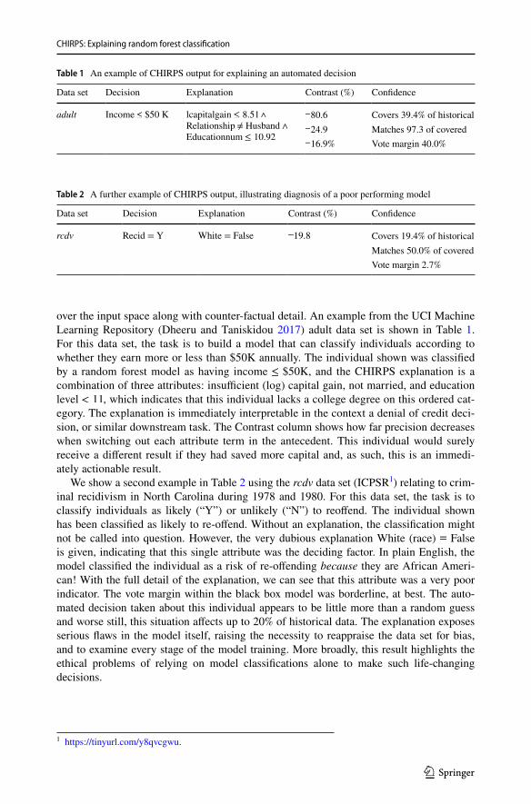
over the input space along with counter-factual detail. An example from the UCI Machine Learning Repository (Dheeru and Taniskidou 2017) adult data set is shown in Table 1. For this data set, the task is to build a model that can classify individuals according to whether they earn more or less than $50K annually. The individual shown was classified by a random forest model as having income ≤ $50K, and the CHIRPS explanation is a combination of three attributes: insufficient (log) capital gain, not married, and education level < 11 , which indicates that this individual lacks a college degree on this ordered cat-egory. The explanation is immediately interpretable in the context a denial of credit deci-sion, or similar downstream task. The Contrast column shows how far precision decreases when switching out each attribute term in the antecedent. This individual would surely receive a different result if they had saved more capital and, as such, this is an immedi-ately actionable result.

We show a second example in Table 2 using the rcdv data set (ICPSR1) relating to crim-inal recidivism in North Carolina during 1978 and 1980. For this data set, the task is to classify individuals as likely (“Y”) or unlikely (“N”) to reoffend. The individual shown has been classified as likely to re-offend. Without an explanation, the classification might not be called into question. However, the very dubious explanation White (race) = False is given, indicating that this single attribute was the deciding factor. In plain English, the model classified the individual as a risk of re-offending because they are African Ameri-can! With the full detail of the explanation, we can see that this attribute was a very poor indicator. The vote margin within the black box model was borderline, at best. The auto-mated decision taken about this individual appears to be little more than a random guess and worse still, this situation affects up to 20% of historical data. The explanation exposes serious flaws in the model itself, raising the necessity to reappraise the data set for bias, and to examine every stage of the model training. More broadly, this result highlights the ethical problems of relying on model classifications alone to make such life-changing decisions.

Table 1 An example of CHIRPS output for explaining an automated decision

Data set Decision Explanation Contrast (%) Confidence

adult Income ≤ $50 K lcapitalgain ≤ 8.51 ∧Relationship ≠ Husband ∧Educationnum ≤ 10.92

−80.6 Covers 39.4% of historical−24.9 Matches 97.3 of covered−16.9% Vote margin 40.0%

Table 2 A further example of CHIRPS output, illustrating diagnosis of a poor performing model


rcdv Recid = Y White = False −19.8 Covers 19.4% of historicalMatches 50.0% of coveredVote margin 2.7%

1 https ://tinyu rl.com/y8qvc gwu.

https://tinyurl.com/y8qvcgwu

J. Hatwell et al.

1 3

To achieve these results, CHIRPS looks at the decision paths taken by the RF to classify a single instance (the explanandum) in each base decision tree (DT) classifier, and retains only those paths that formed the majority vote. This step is justified because a rule based explanation must be locally accurate, meaning that the rule consequent always agrees with the model’s classification (Lundberg and Lee 2017). The minority paths give a different classification and cannot form part of the explanation.

CHIRPS then employs Frequent Pattern (FP) mining to filter only the decision nodes that occur most frequently within the collection of decision paths. The most frequent nodes refer to attributes that contribute the most to the model’s classification. The nodes (or terms) are greedily added into a single classification rule (CR); only the terms that improve the performance against the objective function are added. The “Contrast” analysis in Tables 1 and 2 shows how the rule’s performance deteriorates when we exclude each individual term from the antecedent.

Our experimental study over nine data sets compares CHIRPS with four state of the art methods, that is, Anchors (Ribeiro et al. 2018), Bayesian Rule Lists (Letham 2015a, b), inTrees (Deng 2014) and defragTrees (Hara and Hayashi 2016). These methods generate a rule or cascading rule list (CRL), and so are directly comparable. They are also well cited in the literature. Our results show that CHIRPS is at least as good or significantly better in all quality measures in a comparative study that is broader in scope than much of the previ-ous work in this research area. Furthermore, CHIRPS works well in multi-class problems and class-imbalanced problems, where other methods are inconsistent. Unlike some com-peting methods, CHIRPS does not require discretisation of continuous features as a pre-processing step, and therefore works directly with the model under scrutiny (MUS). We further show that using the traditional objective functions for finding optimal classifica-tion rules—precision and coverage—leads to over- and under-fitting solutions. We suggest novel counterparts that perform better in the local explanation setting.

The remainder of this paper is organised as follows: Sect. 2 discusses related work; Sect. 3 covers key concepts of Decision Trees and Random Forest models; Sect. 4 formal-ises the general problem of explaining classification models and the requirements of an effective solution; Sect. 5 shows how classification rules can be extended to meet all the requirements of explanation; Sect. 6 presents CHIRPS; Sects. 7 and 8 detail our experi-ments and discuss the results; and finally, Sect. 9 concludes the paper and presents some ideas for further work.

2 Related work

In the last decade, many approaches have been taken to ML interpretability. There have been novel model types, designed for interpretability (Letham 2015b; Friedman and Pope-scu 2008; Riiping 2006; Waitman et al. 2006). The advantage of using such methods is early discovery of false assumptions and problems in the data set. Such methods can gen-erate a sparse model that takes advantage of domain knowledge (Rudin 2018). Another approach is to extract an interpretable approximation from an already trained, black box model (Adnan and Islam 2017; Hara and Hayashi 2016; Deng 2014). Although all the methods mentioned so far are very different in their implementation, very many of the resulting models fall into the general category of rule sets or rule lists, especially Cascad-ing (or falling) Rule Lists (CRL). This is because logical rules present an uncomplicated, semantic mapping between the inputs and outputs of classification and are considered by


1 3

many to provide the most intuitive explanations (Wang et al. 2017; Souillard-Mandar et al. 2016; Wang et al. 2016; Wang and Rudin 2015). CRL are ordered sets of classification rules (CR). CR are rules where the antecedent defines regions of the input space and the consequent is the expected class label in that region.

Bayesian Rule Lists (BRL) (Letham 2015a, b) and Brute (Waitman et al. 2006) are two well-known algorithms for generating a CRL directly from data. The objective is to create an interpretable model, as opposed to explaining an existing one. The complete set of CR is extracted from the data set and subjected to Frequent Pattern (FP) mining. Each method employs a probabilistic strategy to return a subset of mined rules of a user-defined, man-ageable size as the final model. Neither method modifies or constructs rules from sub-units. Aside from standard quality measures of the rules (precision and coverage), these methods provide a measure of uncertainty of the rule’s classification. Brute uses several rounds of bootstrapping of the training data to extract CR for the FP mining. Rules that are simi-lar and frequently occurring across replicates are retained, allowing antecedent terms with variance estimates. BRL, on the other hand, uses Monte-Carlo Markov Chains to return a distribution of rule lists. Individual rule lists from the chain can be used as spot estimates, or the distribution can output rules where the consequent is a probability distribution.

The RuleFit algorithm (Friedman and Popescu 2008) is notable for producing a novel rule-based model type, the predictive rule ensemble (PRE). The first step is to generate an intermediate specialised decision forest (DF). The maximum depth of each tree is a small, random integer, resulting in shallow decision trees with high variance that serve as a large pool of engineered, rule-based features. Next, a linear model (LM) is trained using all of the untransformed and engineered features together, while LASSO regularisation (Tibshi-rani 1996) ensures that the LM contains a minimal set of non-zero coefficients. These coef-ficients represent the contribution of the most important features. The rule-based terms in a PRE must be interpreted as oblique (non-orthogonal) parameters whose contribution is counted when the rule covers the instance. Questions remain about the interpretability of such oblique parameters in linear models (Huysmans et al. 2006).

Other methods generate a CRL as a proxy model from an existing MUS (that is always a DF of some kind), as opposed to learning directly from data. This approach is called decompositional (Andrews et al. 1995) because it reduces the search to the smallest infor-mation units of the model (e.g. the inner decision nodes of each base classifier in a decision tree ensemble). The purpose of the proxy is to explain the MUS through a more inter-pretable, simplified structure. The challenge for this approach is to maximise fidelity with the MUS. The related literature shows that such simplified, proxy models inevitably give a classification result that differs from the MUS for a proportion of instances. This phe-nomenon is a consequence of the AITO and such proxy models cannot be used to com-pletely replace the original model. Less than perfect fidelity is a failure to explain individ-ual instances (Rudin 2018); a situation that is unlikely to be acceptable in compliance and safety critical applications. Well known methods in this category include RF+HC (Mash-ayekhi and Gras 2015), ForEx++ (Adnan and Islam 2017), defragTrees (Hara and Hayashi 2016) and inTrees (Deng 2014). Each of these methods extracts all possible rules from root to leaf of each tree in the DF. The inTrees framework then uses FP mining to identify fre-quently occurring rules, while RF+HC and ForEx++ score each rule and apply a heuristic to identify a reduced rule set and defragTrees uses a Bayesian formulation. Based on the experimental results given in the relevant articles, the rule lists for RF+HC and ForEx++ remain too large to be considered truly interpretable. However, the stated aim of ForEx++ is knowledge discovery rather than interpretability per se and the authors further analysed the rule sets for patterns and trends.

J. Hatwell et al.

1 3

Until recently, the interpretability gains of CRL were stated and accepted without much critique (Lipton 2016). However, to classify an instance, a CRL requires a top down evalu-ation; several rules may need to be parsed before finding one that covers an explanandum instance. The resulting explanation is the conjunction of the relevant rule and all preceding rules. Sometimes, there is no covering rule in the list and the model must default to the prior majority class. The interpretation of this default condition is null, “don’t know,” or “the model decided class yk because this is true for the most instances.” It is a trivial and under-fitting result that is unlikely to be acceptable in compliance and safety critical appli-cations. To minimise these undesirable outcomes, a very long rule list may be required, reducing the comprehensibility of the CRL as a whole. So, CRL are straightforwardly interpretable only for easy to classify instances; those that are covered by a rule near the top of the list. A more realistic goal for CRL is to extract general and holistic insights about the model and data as stated in Adnan and Islam (2017), because they have significant dis-advantages for explaining individual classifications. Decision Set based models (Lakkaraju et al. 2016) overcome this limitation, by generating an unordered rule set. As such, a deci-sion set is an OR of ANDs where any one or more rules may resolve to true for an explana-dum (Malioutov and Varshney 2013). These models usually require a user-defined and/or domain informed prior to control the rule cardinality and number of rules generated (Wang et al. 2015); however, the main challenge of these methods is to find the optimal set that maximises coverage while minimising overlap (multiple rules covering the same instances). Overlap requires a tie-break that introduces uncertainty into the classification, while lack of coverage causes a default classification. These problems were recorded on up to 14% of test instances (Lakkaraju et al. 2016), which would be considered much too high for critical applications.

More recently, local explanation methods have emerged that sidestep the AITO alto-gether. They simplify and generalise per instance classifications (Ribeiro et al. 2018; Lund-berg and Lee 2017; Ribeiro et al. 2016; Subianto and Siebes 2007). Local methods implic-itly acknowledge that it is untenable to present a human interpretable view of the entire space of a black box model’s behaviour (Lipton 2016). This approach allows the MUS to be tuned for optimal classification (or prediction) accuracy without being compromised by the explanation process; that is, there is no loss of fidelity. Several local methods have been proposed in a model-agnostic framework, probing the model’s behaviour without needing to access the internal representation. They learn how the model’s output changes over a perturbation distribution in the locality around the explanandum (according to some distance metric) and infer the importance of varying the inputs from the resulting output values. This approach, of learning from the model’s behaviour, is described as didactic (Andrews et al. 1995). LIME (Ribeiro et al. 2016) is perhaps the most popular of these methods since its publication and recently Shapley values (Lundberg and Lee 2017) has also gained attention. These methods assign a real value to the most important attributes, hence are known as Additive Feature Attribution Methods (AFAM). An AFAM explana-tion is equivalent to a surrogate LM that approximates the behaviour of the classifier at the locality of the explanandum. The largest coefficients indicate largest contribution to the model’s classification or prediction. LIME and Shapley Value explanations are intuitive for the end user, thanks to well-designed graphical outputs. However, it is not easy to know when one instance’s explanation applies to other instances. This limitation was overcome in Anchors, which is a very recent extension to LIME. Anchors returns a single rule as an explanation, illustrating the enduring importance of logical rules despite the paradigm shift towards local explanations. Relevance of an explanation to other instances is deter-mined unambiguously; either the rule is covering the new instance or it is not. Anchors


1 3

and LIME require all features to be discrete, and internally pre-process any continuous features into quartile bins by default, which can result in loss of information. These tech-niques have been shown to be effective in image and text classification but there are some limitations when applied to tabular data sets (Michal 2019). As described in Ribeiro et al. (2018) and Ribeiro et al. (2016), the perturbation distribution must be estimated from the joint distribution of the source data and this requires access to the training data set. In other words, these model-agnostic methods are not data-agnostic! If access to the training set is assumed, then the model-agnostic assumption of accessing only the inputs and outputs of the black box model is violated. This problem is overcome in LORE (Guidotti et al. 2018), which uses a genetic algorithm to generate a population of instances and allows for a worst case scenario where only information about the permissible range of values for each fea-ture in the input space in known. This approach, however, is limited to binary classification and can take a prohibitively long time to run. Also, all of these local sampling techniques have been shown to introduce uncertainty and explanations with high variance for similar instances (Fen et al. 2019). This means they require additional checks to determine whether the selected attributes and features are stable over repeated trials. These results suggest that the model-agnostic assumption should be taken with caution.

We argue that the model-agnostic assumption is only required for a subset of problems in the context of HIL processes, such as model auditing by an external third party. HIL pro-cesses are frequently found in settings where the model and its training/test data are owned by the explainee. For example, a financial services company segmenting its loan applica-tions by risk, or a medical enterprise implementing automated diagnostics. In these cases, there is no imperative to use a model-agnostic method, especially if a different approach gives better insight. Another problem with model-agnostic is that they explain correlations in the synthetic sample, but not necessarily what the black box model computes (Rudin 2018). This problem calls for a decompositional approach that explains each data instance separately and reveals the internals of the black box.

The very notion of interpretability in ML has been frequently ill-defined in the ML lit-erature, with serious attempts at scientific rigour only appearing very recently (Doshi-Velez and Kim 2017; Bibal and Frenay 2016; Lipton 2016; Subianto and Siebes 2007). Taking an inter-disciplinary approach and drawing from the social sciences, Miller (2017) sets forth guiding principles for a form of explanation that reflects how people explain actions and reasoning to one another. Several other sources confirm that this is a desirable quality

(Woodward 2017; Wilkinson 2014; Salmon 1971; Hempel and Oppenheim Apr. 1948). These guiding principles suggest that explanations should be:

• minimally complete—neither under- nor over-fitting;• contrastive—providing information about counter-factual cases;• and a model of self—referring to historical data, not obscure parameters or synthetic

distributions.

This research contributes a formalisation of explanations that align with these principles. Furthermore, our proposed method is the first explanation method to our knowledge that addresses directly the above principles. By relaxing the model-agnostic assumptions and given the realities of supervised learning on tabular data sets, our method offers the best of decompositional and didactic methods. Our rule-based explanations have no loss of fidel-ity, unlike global methods. When tested on unseen data and compared to state of the art methods, the rules are also more precise without tending to over-fit, and have higher cov-erage without tending to under-fit. These properties produce excellent robustness to class

J. Hatwell et al.

1 3

imbalance where other methods struggle. Aside from LORE (Guidotti et al. 2018), ours is the only method to enhance the explanation with information about counter-factual cases but our method naturally addresses multi-class problems and classification uncertainty, while LORE only targets binary classification problems.

3 Decision trees and random forests

Before presenting our method in detail, we provide a brief overview of Decision Trees (DT) and, more specifically, the Classification and Regression Trees (CART) algorithm. CART models are the DT variant used in the original Random Forest (RF) algorithm (Bre-iman 2001). The CART algorithm is a heuristic method for inducing DT by top-down, greedy, recursive, and binary partitioning of the training data set. CART induction begins with a single (root) node that covers all training data instances. Using non-class attributes, CART proceeds by generating decision nodes that separate the instances into increasingly pure partitions according to their class label. On each iteration, candidate splits are evalu-ated for all nodes that are currently at the end of a decision path but do not yet meet the stopping criteria. The candidate split that would generate two child nodes with the lowest weighted total Gini Impurity IG is always chosen and those child nodes are then added to the growing tree:

where pk is the proportion of instances having label yk in a node Q and K is the number of classes.

where {Qfirst,Qsecond} is the set of child nodes that would be created by the candidate split and |Q| is the number of training instances covered by a node. This action occurs indepen-dently from any previous or subsequent iteration. There is no way to back out a previous move or find better splits by considering feature interactions. As such, this typifies a greedy heuristic; it is much more computationally efficient than an exhaustive search but has no guarantee of finding the optimal DT. The method is deterministic for a single tree and a static sample.

To classify a previously unseen instance, simply follow the path of that instance down the tree, beginning at the root and obeying the split condition of each decision node until a leaf node is reached. The split conditions are binary conditions that are either true or false for an instance. So, every instance can follow one and only one path, and arrive at one and only one leaf node. Each leaf node covers a subset of the training instances and returns the majority class label of those instances as the classification. See Fig. 2.

A RF is an ensemble of, typically, tens to thousands of base DT classifiers. The ensemble operates in parallel and classifies by majority vote. This improves classifica-tion performance in an ensemble compared to a single classifier, assuming each classi-fier in the ensemble performs somewhat better than a random guess and they are diverse (if not completely uncorrelated) in their errors. In an ensemble, erroneous classifica-tions are outnumbered by correct classifications with very high probability, resulting in

(1)IG(Q) =

K∑

k=1

pk ⋅ (1 − pk)

(2)Weighted Total IG =IG(Qfirst) ⋅ |Qfirst|

N+

IG(Qsecond) ⋅ |Qsecond|N


1 3

a correct classification on aggregate. To promote the required structural diversity among the base classifiers, stochastic processes are introduced at two stages of DT induction. Firstly, each DT is induced on a uniform sample with replacement (bootstrap) of the training data set. Secondly, although it is still always the best IG scoring candidate split that is added to the tree on each iteration, the candidate splits are limited to a ran-dom sub-sample of possible candidates. In other respects, tree induction is the same as described in earlier paragraphs except, to further increase the structural variance, it is common to avoid applying any stopping criteria. Under these conditions, trees are fully grown so that their leaves are pure; each leaf covers training instances of only a single class. The resulting trees can be very deep and bushy and individually over-fitting yet, as an ensemble, RF models constructed this way are highly competitive for accuracy among widely available ML methods (Fernandez-Delgado 2014) and are also robust to over-fitting (Breiman 2001), class imbalance, noise, non-informative features, anoma-lies and variations in the source data (Vens and Costa 2011), and more able to discover useful feature interactions over the whole sample of random trees. There are only two tuning parameters that control most of the variation in performance: the number of trees and the number of candidate features used to generate candidate splits. These proper-ties make RF easy to deploy and popular in practice. In contrast to the relatively simple structure of an individual DT, the consensus is that RF are typical examples of uninter-pretable, black box models; Breiman, the inventor of the original RF, described them as “impenetrable” (Breiman 2001). There are several methods for extracting a general measure of feature importance (Gain, Split Count, Permutation Error) but these deliver inconsistent results (Lundberg et al. 2017). Furthermore, these measures can only com-municate that certain features were more useful in delivering the model’s overall accu-racy or error scores. This falls short of providing explanations that detail the contribu-tion of specific attribute values to the classification output or determining the effect of changing the inputs to generate counter-factual classifications.

4 Problem formulation

Interpretability of ML models has been poorly defined in the ML literature until recently (Lipton 2016). In response, this section presents our requirements for local explana-tions, based on the guiding principles proposed in Miller (2017). We also scope these definitions to classification problems on tabular data sets.

Fig. 2 To classify an instance � = {… , xi = 0.1, xj = 10, …} , we start at Q1 and follow the binary split conditions until we reach a leaf node, Q6 in this case, which returns the label yk to the caller

J. Hatwell et al.

1 3

4.1 The problem of classification

Let X ∈ ℝP be a feature space where P ∈ ℕ is an arbitrary number of features. The jth

feature is Xj . An instance space � ∈ X of N ∈ ℕ instances is an N × P matrix. Instance �(i) = [x

(i)

1,… , x

(i)

P] is the ith row vector of � and �j = [x

(1)

j,… , x

(N)

j]T is the column vec-

tor of the jth feature. An attribute x(i)j

is the value at the jth feature of the ith instance. Let Y = {y1,… , yK} be the space of K possible class labels, and � ∈ Y be a vector of length N of known instance labels. There is an unknown, conditional distribution f = F(y|�) such that any randomly sampled, labelled instance space (�,�) has the joint distribution F(�, y) = F(y|�) ⋅ F(�) . A classifier is a known function g ∶ X ⟼ Y, g ∈ G selected from the hypothesis space G by empirical risk minimisation (Vapnik et al. 1998) over a given, labelled instance space (�,�) , such that g approximates f and is expected to generalise to any random instance space, sampled from the same distribu-tion: g(�) ≈ f (�), � ∈ X

4.2 The problem of explaining classifications

In Sect. 5 we will show that CR suit explanations; however, CR may not be the only valid or useful choice. Therefore, in this section we first build a theoretical framework for expla-nations in general. To aid the reader, we provide Table 3 as a key to the notation used that introduces new concepts in the remainder of this article.

We seek a function e ∶ G, x ⟼ E whose output is E = e(g, �), E ∈ Eg� , where Eg� is the space of possible explanations for a single black box classification event g(�) . E must be optimal for reliability, generality and interpretability. The trade-off between reliability and generality weighs upon most ML research but interpretability adds several dimensions. It is very difficult to define a general form for explanations that could apply to all situations (all hypothesis spaces and problem spaces). Measuring whether and how much a given E is informative requires the use of proxies that can only be compared between solutions of the same class, such as the number of non-zero linear coefficients (linear models), rule cardi-nality and number of rules (rule-based models), maximum tree depth or number of nodes (decision trees), number of support vectors in SVM (Bibal and Frenay 2016; Garcia 2009), or the number of relevant features from a tabular data set. This is not always satisfactory in high dimensional problems (Lipton 2016).

We identify the following requirements:

Requirement 1 E must be minimally complete. We want E to have the smallest possi-ble dimension dim(E) (perhaps measured as the above mentioned proxies). This require-ment means that E must be the smallest subset of useful information encoded in (g, �) that maximises both reliability and generality. Consider, however, a classification task with class imbalance. A trivial or null explanation—one that states that the majority class was selected but gives no reasoning—could apply to every instance (maximum generality) and be valid for all the instances that receive the majority class label from the model (very high reliability). This situation is erroneous because it explains the classification event without any reference to the model’s encoding of attribute differences between the classes—the relationship between � and � . The implication is that all input values lead to the target


1 3

class, which is false. This is an under-fitting scenario, equivalent to a classification model with constant output. So, E must reduce the problem dimensionality but must remain informative to some extent; E may not be trivial.

Requirement 2 There must be some function r that determines when E = e(g, �) is rel-evant to any instance other than the explanandum instance � in the reduced dimension of the solution space Eg� (Req 1):

where � ≠ � , � ∈ X and a ⊧ b ( a models b ) means a is a logical conjunction and every part of a is true of b. Thus, the relevance subspace of E can be determined from r:

Note, E ∈ Eg� means that E is an explanation of � , therefore r(E, �) = 1 and � ∈ ZE are always true.

(3)r(E, �) =

{1 if E ⊧ �

0 otherwise

(4)ZE = {� ∶ r(E, �) = 1, � ∈ X}, ZE is continuous.

Table 3 Summary of notation

Symbol Definition

N The number of instancesP The number of predictors/featuresK The number of classese(g, �) A function that generates an explanation from a classifier and an instanceEg� The space of possible explanations that e(g, �) can returnE A concrete example of an explanation from Eg� ; the output of e(g, �)dim(E) Returns the dimension of E e.g. rule cardinality, non-zero coefficients etc�(a) Returns the binary truth of its argumentℙ(a) Returns the probability / proportion of its argumentL(a, b) Returns the zero-one loss of its argumentsr(E, �) A relevance function that determines if E generalises to an instance �ZE An input subspace of the input space X over which E generalises�E An instance subspace of the data set � over which E generalisesR(E) Local risk—the expected loss of E over ZE

Remp(E) Local, empirical risk—the estimated loss of E over ZE

Z′

EThe counter-facutal relevance subspace of E

�′E

The counter-factual instance subspace of Eclwrj, c

upr

jLower and upper bounds defined over a feature j

CZEA set of upper/lower bounds that define the relevance space of E

� (g,�E , �) Stability—a precision-like quality measure for explanations�(g,�,�E , �) Exclusive coverage—a coverage-like quality measure for explanations(j, �, �) Detail of a given node in a decision path: a triple of (feature index,

threshold value, Boolean test)psn A given path snippet, comprising one or more node detail triples� A user-defined target stability. An early stopping parameter

J. Hatwell et al.

1 3

Requirement 3 E must have maximal local reliability. The term local refers to everything inside the relevance subspace. Perfect local reliability means that g(�) = g(�), � ∈ ZE but this may not be possible while simultaneously satisfying minimal completeness. We can proceed by minimising local risk:

Typically in ML research, the true distribution of � is unknown. Therefore, the risk must be estimated empirically from an instance space � of observed data. � could be the train-ing set used to train g or any i.i.d. random sample from the same distribution. The relevant instance space is:

Then, empirical local risk can be estimated by:

which is related to precision, by way of reversing the zero-one loss function:

where the final term is equivalent to the standard definition of precision.

Requirement 4 E must be as general as possible given maximal local reliability. This means its relevance subspace covers the largest continuous volume of the feature space that achieves the same precision or better than any other relevance subspace. The E that satis-fies this requirement meets the following criteria:

Requirement 5 E must not be tautological, meaning that it generalises to a set of instances not limited to the singleton explanandum � . An E that does not generalise beyond the sin-gleton � is an erroneous situation that trivially explains the classification event g(�) by the uniqueness of � in the data set. This is the local explanation equivalent of over-fitting. Such over-fitting could arise at a complex or noisy decision boundary. In the most extreme case, where g(�) = yk while for every near neighbour g(�) ≠ yk , equation (8) is trivially max-imised if � is the only member of �E and plummets when any � ≠ � is included in �E . In Sect. 5, we introduce a novel objective function, stability to gracefully handle this problem.

(5)R(E) =∫

L(g(�), g(�)

)d�, � ∈ ZE, E ∈ Eg�,

(6)L(a, b) =

{0 if a = b

1 if a ≠ b

(7)�E = {� ∶ � ∈ ZE ∩ �}.

(8)Remp(E) =1

|�E|

|�E|∑

i=1

L(g(�(�)), g(�)

); �(�) ∈ �E, E ∈ Eg�,

(9)

ℙ(g(�(i)) = g(�)

)=(1 − Remp(E)

)

=1

|�E|

|�E|∑

i=1

1 − L(g(�(�)), g(�)

)

=1

|�E|

|�E|∑

i=1

𝕀(g(�(�)) = g(�)

); �(�) ∈ �E, E ∈ Eg�

(10)|�E| > |�E� |, ℙ(g(�E) = g(�)

)≥ ℙ

(g(�E� ) = g(�)

), E ≠ E�, E,E� ∈ Eg�.


1 3

Requirement 6 It must be possible to present E with contrastive, counter-factual informa-tion. That is, we assume that the form of explanation reveals the minimal changes to the inputs that give different results. In Sect. 5 we show how this is defined for CR specifically. Some authors posit that the counter-factual cases are any changes in the attributes of an instance that would result in a different classification (Guidotti et al. 2018; Subianto and Siebes 2007). However, such a definition can only apply to discrete, nominal and deter-ministic predictors. In the case of continuous predictors with complex decision boundaries, such as the mixed Gaussian process shown in Fig. 4, there could be several non-contigu-ous or interleaved regions of the input space (Ho and Basu 2002) that classify identically; in these cases a change of the minimal attribute set may not always result in a different class assignment. We can, however, expect a change in precision outside the relevance space and there is support for such models that offer measures of uncertainty rather than crisp boundaries in the literature (Proenca and Leeuwen 2019; Letham 2015a, b; Wait-man et al. 2006). Therefore, we propose a task dependent definition of contrastive explana-tions: counter-factual cases should be demonstrably different from observed cases. This difference is manifested as a drop in precision below some user-defined tolerance � . That is ℙ(g(��

E) = g(�)

)≤ ℙ

(g(�E) = g(�)

)− � where

This quantity is the precision of the counter-factual instance space �′E , and Z′

E is the

counter-factual relevance space. Note, Z′

E is a space, or set of spaces covered by minimal

changes to E. It is not equivalent to {� ⧵ ZE} , which is the entire input space not covered by E. If the latter were true, then each unique explanation would be a global model describ-ing the entire input space by itself and its complement. Rather, the benefit of counter-fac-tual information is to identify the boundary outside which E is no longer reliable.

Requirement 7 E should be a “model-of-self” that explains the model from the data. Model g is the output of a learning algorithm (a function) that was parameterised by the training data (�,�) . E should frame the explanation in terms of the influence of (�,�) over the original learning algorithm. This requirement is met de facto by the empirical formula-tions given.

In the following sections, we show how CHIRPS using CR as the form of explanation, is designed to meet these requirements. As our experimental study shows, competing meth-ods that do not explicitly address them all have a tendency to converge to under- or over-fitting solutions.

5 Extending classification rules as explanations

Frequent Patterns (FP), Association Rules (AR) and Classification Rules (CR) are all modes of expressing relationships between patterns in a data set. A pattern is formed from k ≥ 1 attributes, and referred to as a k-item set. The support count = �(fp) is the number of instances in a data set that match the pattern fp, while support(fp) = �(fp)

N is the fraction of

instances containing fp. A pattern is said to be frequent if its support exceeds minsup, a user-defined threshold. AR describe associations over the whole data set between

(11)

ℙ(g(��

E) = g(�)

)=

1

|��E|

|��E|∑

i=1

𝕀

((g(�(i)) = g(�)

)), �(i) ∈ �

�

E, ��

E= {� ∈ Z

�

E∩ �}

J. Hatwell et al.

1 3

individual items within a k > 1 item set. For example, for a 2-item set fp = {Z, Y} , there is a relationship expressed as the rule: Z ⟹ Y . Here, Z is called the antecedent and Y the consequent. Such an AR has a level of confidence or precision, which is equal to the condi-tional probability ℙ(Y|Z) = support({Z,Y})

support(Z) , where support(Z) = ℙ(Z) is the support of the

antecedent alone (also called the coverage). A CR is simply an AR where Z is a set of con-ditions defined on one or more features {X1,… ,XP} of a data set, and Y is a class label. It is trivial to derive a CR from the decision path of a DT (Quinlan 1987): Using the example from Fig. 2, the following is a CR:

5.1 Meeting the requirements for explanations

We can find CR that conform to our formulation of an explanation, given in Sect. 4, if we set Z = ZE , a relevance subspace, and Y = g(�) , the output of the model. Then, the CR is simply ZE ⟹ g(�) . Req 2 is satisfied by this formulation because we can define the rel-evance evaluation function as:

where CZE is the set of parameters that define the lower and upper bounds of each feature.

For a feature space with P features, any {clwrj, c

upr

j, j ∈ P} may be undefined, in which case

the interval begins and/or ends with the domain of Xj . Minimising dim(E) requires |CZE| to

be as small as possible, though it may not be zero (Req 1). The best case is |CZE| = 1 and

the worst case is |CZE| = 2P.

To find candidates E ∈ Eg� that meet the requirements, we propose an iterative, breadth-first search heuristic as follows: at iteration i = 0 , E(i) is a trivial or empty rule. In other words, the antecedent CZ

E(0)= ∅ while the consequent is g(�) . Thus coverage is complete

at the start and will be iteratively reduced in a trade off (Req 4) with precision. In each subsequent iteration i + 1 we either add a new parameter or update an existing one that strictly increases the precision. However, to avoid tautological solutions (Req 5), we cannot use high precision as an optimisation target for this procedure because this measure can be trivially maximised with singletons or very small, overfit subspaces. We therefore propose stability, a novel objective function that penalises explanations that explain only a small number of instances.

Definition 1 Stability takes the form � ∶ G,X, x ⟼ ℝ ∈ (0, 1).

where K is a regularising constant and equals the number of possible classes.

The middle formulation in equation (14) shows how this measure relates to requirement 5; we calculate the precision of g(�) = g(�) inside the relevant instance space, excluding

(12){� ∶ min(Xi) ≤ xi < 0.5, 8 ≤ xj ≤ max(Xj)} ⟹ yk

(13)r(E, �) ∶=

P∏

j=1

�

(max

(clwrj, min(Xj)

)≤ zj ≤ min

(cupr

j, max(Xj)

)),

clwrj, c

upr

j∈ CZE

, � ∈ X

(14)

� (g,�E, �) =|{� ∶ g(�) = g(�), � ∈ �E ⧵ �}| + 1

|�E| + K=

|{� ∶ g(�) = g(�), � ∈ �E}||�E| + K


1 3

� itself. We apply additive smoothing as n+1m+K

. Then, the numerator simplifies as shown in the final form. Therefore, stability is similar to using precision with a Laplace correction (Clark and Boswell 1991) but with a more severe penalty. Due to the division by K, trivial relevance spaces (of size 1) only get a stability of 33% or less for K ≥ 2 . The function pro-file shown in Fig. 3 makes this clear.

We illustrate the benefit of this novel function with an example given in Table 4. At iteration i, there are twenty-one covered instances � ∈ �E(i) . For all but one of these g(�) = g(�) . This could be an optimal solution but the search continues to iteration i + 1 . The rule takes a new, more specific parameter and �E(i+1) now covers just one instance. If we are optimising for precision, E(i+1) would be considered better than E(i) because preci-sion is trivially maximised to 1.0. Stability, on the other hand, has fallen well below any tolerable level, so instead we keep E(i) as the explanation. It is important to realise that better recognised statistics such as recall and F-1 measure are unsuitable in this setting; since, the table shown in the examples is not a confusion matrix. Rather, we have tabu-lated the instance classification versus the rule coverage. We seek to maximise covered, target class and minimise covered, other class. We can tolerate high numbers of instances in the not covered column because we assume these instances will be covered by another explanation. Another perspective is that stability approaches precision asymptotically

Fig. 3 Maximum achievable stability (the discrete points) when all instances are given the same classifica-tion, for relevant instance spaces containing from one to forty instances and K ∈ {2, 3, 4} . The dashed line shows precision, which is always exactly 1.0 in these circumstances, no matter how small the instance space

Table 4 Demonstrating stability for K = 2 with examples

Rule-instance table Measure Values

Covered Not covered

Iteration iTarget class 20 780 Stability 0.870Other class 1 199 Precision 0.952

Recall 0.025F−1 0.049

Iteration i + 1

Target class 1 799 Stability 0.333Other class 0 200 Precision 1.0

Recall 0.001F−1 0.002

J. Hatwell et al.

1 3

as |�E| → ∞ but when |�E| diminishes so does the maximum stability; maximum stability = 1

K when |�E| = 1 . This behaviour acts as a brake that prevents the algorithm

from adding more parameters and converging on singletons. This is achieved non-paramet-rically, without the need for user intervention.

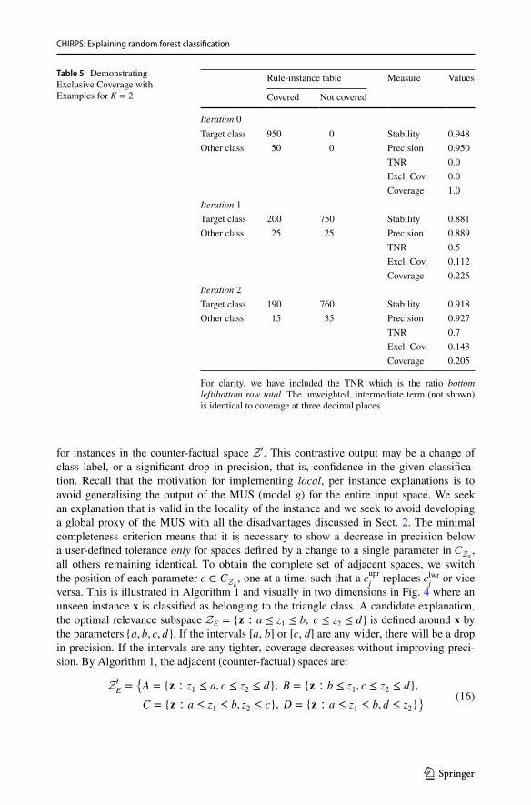
We introduce another, novel quality measure by returning to the minimal complete-ness requirement (Req 1). This states that there must be at least one informative parameter that can distinguish between differently classified instances. In situations of severe class imbalance, precision and coverage could simultaneously be trivially maximised by a null solution that covers the entire input space. As we show in our experimental results, class-imbalance can lead to such under-fitting solutions in several competing methods. To guard against this, we propose a further, novel objective function, exclusive coverage in equation (15) that penalises high coverage against a lack of discrimination between classes.

Definition 2 Exclusive coverage takes the form � ∶ G,X,X, x ⟼ ℝ ∈ (0, 1) . Exclusive coverage is calculated as coverage, the fraction of all instances covered by the rule exclud-ing the explanandum. This is similar to the relation between stability and precision. Addi-tionally, however, the value is weighted by the ratio of not covered, other class to not cov-ered, other class + covered, other class (equivalent of “true negative rate”). This measure increases with the number of differently classified instances outside the relevant instance space �E.

where TNR is the so-called “true negative rate” described above.

We illustrate the benefit of this novel function with an example given in Table 5. In this highly imbalanced class example, at iteration 0, the null rule covers all instances. Precision and stability are very high, perhaps above a threshold that could trigger an early stopping condition. Coverage is trivially maximised at 1.0. To report such a result would lead to a misleading representation of the rule quality. It is clearly an under-fitting solution. So we must add a term to the rule, even one that may dramatically decrease stability, precision and, of course, coverage. An example of a possible subsequent state is shown at iteration 1. At this point, the search for additional rule terms that can increase stability should con-tinue. So, at iteration 2, another rule term is added. This results in a more specific rule that has slightly reduced coverage, but slightly increased exclusive coverage. This example shows how using exclusive coverage as a quality measure helps to disqualify under-fitting solutions.

We reiterate the importance of using appropriate quality measures for explanations and how these differ from measures typically associated with classification accuracy (precision, recall, F-1 score). These novel functions are central to the contribution of this research.

5.2 Providing contrastive and counter‑factual information

Counter-factual examples illustrate changes in the inputs that will give different results. We have defined this in Req 6 as ensuring that the MUS’s outputs are demonstrably different

(15)𝜉(g,�,�E, �) = TNR ⋅

|�E ⧵ �| + 1

|�| + K= TNR ⋅

|�E||�| + K

, �E ⊆ �

TNR =|{�� ∶ �

� ∉ (�E) ∧ g(��) ≠ g(�)}||{� ∶ � ∈ (�) ∧ g(�) ≠ g(�)}|


1 3

for instances in the counter-factual space Z′ . This contrastive output may be a change of class label, or a significant drop in precision, that is, confidence in the given classifica-tion. Recall that the motivation for implementing local, per instance explanations is to avoid generalising the output of the MUS (model g) for the entire input space. We seek an explanation that is valid in the locality of the instance and we seek to avoid developing a global proxy of the MUS with all the disadvantages discussed in Sect. 2. The minimal completeness criterion means that it is necessary to show a decrease in precision below a user-defined tolerance only for spaces defined by a change to a single parameter in CZE

, all others remaining identical. To obtain the complete set of adjacent spaces, we switch the position of each parameter c ∈ CZE

, one at a time, such that a cuprj

replaces clwrj

or vice versa. This is illustrated in Algorithm 1 and visually in two dimensions in Fig. 4 where an unseen instance � is classified as belonging to the triangle class. A candidate explanation, the optimal relevance subspace ZE = {� ∶ a ≤ z1 ≤ b, c ≤ z2 ≤ d} is defined around � by the parameters {a, b, c, d} . If the intervals [a, b] or [c, d] are any wider, there will be a drop in precision. If the intervals are any tighter, coverage decreases without improving preci-sion. By Algorithm 1, the adjacent (counter-factual) spaces are:

(16)Z

�

E={A = {� ∶ z1 ≤ a, c ≤ z2 ≤ d}, B = {� ∶ b ≤ z1, c ≤ z2 ≤ d},

C = {� ∶ a ≤ z1 ≤ b, z2 ≤ c}, D = {� ∶ a ≤ z1 ≤ b, d ≤ z2}}

Table 5 Demonstrating Exclusive Coverage with Examples for K = 2

For clarity, we have included the TNR which is the ratio bottom left/bottom row total. The unweighted, intermediate term (not shown) is identical to coverage at three decimal places

Rule-instance table Measure Values

Covered Not covered

Iteration 0Target class 950 0 Stability 0.948Other class 50 0 Precision 0.950

TNR 0.0Excl. Cov. 0.0Coverage 1.0





J. Hatwell et al.

1 3

Provided the precision of the explanations representing each of these subspaces falls

below the user-defined tolerance, all the requirements are satisfied. If a counter-factual space has a precision above the tolerance, the space can be merged with ZE by removing the defining parameter from the rule antecedent.

6 CHIRPS

We propose our novel procedure to search for CR that meet the requirements for local explanations. CHIRPS is a concrete implementation of the function e(g, �) and the heu-ristic search introduced in Sects. 4 and 5. CHIRPS assumes g is a random forest model, which defines CHIRPS as a model-specific method. Each step is illustrated in the con-ceptual diagram in Fig. 5 and detailed in the following sections. To explain the clas-sification of an unseen instance, the original training set can be used in the rule finding step. The test set, originally used for assessing the classification accuracy of g, can be used to verify quality of the resulting explanations, using a leave-one-out procedure: One instance is classified and explained, while the remaining instances are kept aside and contribute no information to the explanation. These remaining instances can then be

Fig. 4 A model with a complex boundary trained on a synthetic data set which has two classes, shown as triangles and circles and the candidate relevance space ZE is defined by four parameters a, b, c and d


1 3

used to determine stability and exclusive coverage scores for that individual rule. Thus each instance of the test set constitutes an experimental unit. Performance of an expla-nation algorithm is then the aggregate score over all these units.

6.1 Path extraction and filtering

The first step is to classify the explanandum instance � and simultaneously extract the decision path of every DT. This is simply a matter of tracking the detail of each node. Without loss of generality, the node detail can always be posed as the evaluation of an inequality xj < 𝜈 , where j is a feature index and � ∈ ℝ . Let � ∈ {0, 1} be the binary truth of the evaluation. Thus, each node detail is the triple (j, �, �) . Assuming nominal values are binary encoded, we can represent node detail for any data type with this structure. The interpretation depends on the domain of Xj . The following examples are for illustra-tive purposes and are non-exhaustive:

There is only one possible path for � down each tree so the rest of the model is ignored (of course, for a different instance, a different set of paths are extracted). Trees have a number of nodes in O(2n) where n is the maximum tree depth, compared to paths that are O(n) , so this step reduces the search space logarithmically while retaining all the information about g(�) . A second level of filtering is achieved by retaining only decision paths that agreed with the majority vote. Trees that voted for a minority class represent noise in the model. Their contribution was made redundant by the majority vote system.

(17)

(i, 0.5, 1) ∧ Xi ∈ {0, 1} ⟹ xi = 0 (binary false)

(j, 0.5, 0) ∧ Xj ∈ ℝ ⟹ 0.5 ≤ xj ≤ max(Xj) (real valued interval)

(l, 3.5, 0) ∧ Xl ∈ {1, 2, 3, 4, 5} ⟹ xl ∈ {4, 5} (likert score ≥ 4)

Fig. 5 Conceptual diagram of CHIRPS in four steps: A. Path Extraction and Filtering, B. FP Mining, C. Scoring and Ranking, D. Merging and Pruning

J. Hatwell et al.

1 3

6.2 Frequent pattern mining

In this section, we explain how FP mining is very well suited to extracting knowledge from random forests. Treating the RF model as a sample of a tree-structured random variable, certain stochastic phenomena have been demonstrated (Paluszynska 2017; Louppe 2017; Biau 2012; Vens and Costa 2011; Ishwaran 2007). As described in Sect. 3, CART adds decision nodes to a growing tree that minimise the total, weighted IG score on each itera-tion. Therefore, features with the greatest power to discriminate between classes occur with greatest probability at shallow levels because they are selected whenever they appear as candidates. This results in a smaller mean depth of nodes involving those features. Every root node in the RF has probability p = 1 of being included in the set of decision paths of any instance. The probability of being included falls exponentially with each tree level because the number of alternative paths grows at O(2n) for n levels. So nodes involving the most discriminating features will appear in the collection of paths with very high probabil-ity. Also, the weighted total IG of a candidate split is conditional on all nodes above it in the same path. This means that features that interact have a greater chance of co-occurring in any given path, with these co-occurrences showing increased frequency over the whole collection. These properties suggest that frequency based filtering will be very effective at selecting the most important decision nodes. Furthermore, instances with more attributes in common are more likely to follow a similar path through each tree, resulting in solutions that are highly generalisable.

In addition to the above properties, note that FP mining requires a transaction list as input. A transaction list is a very suitable representation for the set of extracted and filtered decision paths. Each decision path can be considered as a transaction. Each transaction is a set of items, being the triples (j, �, �) described in the previous section. The whole triple is the underlying unit for pattern matching. To execute a reasonable FP-mining task of these units, it is necessary to resolve the potentially very large num-ber of unique values resulting from real-valued features. The cut-point � chosen inde-pendently by each DT might be anywhere in a location that separates the classes. That is to say, many unique values may all represent the same decision boundary. So, this uniqueness presents a problem. Before performing the FP mining, all triples matching (j, ∙, �)—where ∙ is any value—are discretised. This is illustrated in Fig. 6. Increasing

Fig. 6 Simulation of discretising by the median (solid line) of twenty axis aligned splits (dashed lines) that all represent the same decision; they are sampled uniformly from inside the margin between two clusters that are linearly separable on continuous feature X1


1 3

the number of discrete values may improve results with more complex boundaries, so we use a binning function where number of bins can be set as a user-defined tuning parameter.

The output of FP mining is a list of FP that exceeded the minimum support, further filtering the search space prior to the rule building step. The support value of each item set is also returned as a score. Since these k-item sets may represent non-contiguous nodes in a path, we name these objects high importance random path snippets or sim-ply, path snippets.

6.3 Ranking

Even though the previous two steps have dramatically reduced the search space, find-ing the minimal set of snippets that maximises stability and exclusive coverage is a multi-objective, combinatorial problem. To avoid an exhaustive search we rank the snippets according to a heuristic score. The RF+HC method (Mashayekhi and Gras 2015) also uses a score function for rule ranking, so that function was considered first. Unfortunately, it demonstrates undesirable behaviour for our needs. Firstly, the penalty increases with rule length because rule length appears in the denominator. This is the wrong direction because, under FP mining, higher cardinality snippets naturally have lower support than those with lower cardinality (Agrawal et al. 1994). Those longer snippets that have passed our support threshold contain the most useful feature inter-actions. Secondly, the penalty depends on rule accuracy and coverage because the number of covered and correct instances appear in the numerator. We need to separate these effects. Consequently, we developed a unique ranking system that uses cardinal-ity adjusted support with regularisation.

where ps is the path snippet, | ∙ | is the cardinality, or length of ∙ and the remaining vari-ables are tunable parameters:

• sup ∈ {1, support(ps)} . If set to 1 then the effect is neutral.• � is a real valued constant to adjust the support based on path snippets cardinality.

Higher order interactions are favoured when 0 ≤ � . The effect is neutral when � = 0

.• w is a regularising weight (with a neutral default = 1 ). Our early investigations indi-

cated that performance improved when each ps ’s score was weighted by the follow-ing Kullback-Leibler (KL) Divergence:

where P, Q are the posterior class distribution when each snippet is used to partition the training data, and prior class distribution, respectively. The KL-Divergence meas-ures the information lost if a distribution Q is used, instead of another distribution P to encode a random variable. Our sensitivity analysis shows that the use of this weight reduces the variance of stability for a large sample of test instances (see Sect. 8.2).

(18)Score(ps,w, sup, �) = w ⋅ sup ⋅(|ps| − �)

|ps|

(19)wps = DKL(P ∥ Q) = −∑

x∈X

P(x) log

(P(x)

Q(x)

).

J. Hatwell et al.

1 3

6.4 Merging and pruning

Following the heuristic steps outlined in Sect. 5, the path snippets from the ranked list are merged into a CR using a simple, greedy algorithm. Section 7 details our experimental results, showing that this solution is fast and beats competing methods without requiring a more sophisticated optimisation algorithm. A walk-through of the major steps is given here. Also, see Algorithm 2.

Step 1 Starting breadth first with a non-informative, null explanation:

where i is the iteration number. The initial relevance subspace has no defining parameters and so covers the entire input space X and the relevant instance space �E(0) = � is equal to the entire training set. The prior stability s0 can be a point estimate: � (g,�E(0) , �) , or esti-mated with confidence intervals using the bootstrap: 1

B

∑B

b=1� (g,�∗b

E(0), �) , where B is the

number of bootstraps and �∗b

E(0) is the bth bootstrap sample of the relevant instance space.

Step 2 On each iteration i, a candidate subspace is formed from CZE(i−1)

∪ ps1 where ps1 is the path snippet currently at the top of the ranked list. The stability of the candidate and current subspaces are compared, using the bootstrap formulation:

If p exceeds some confidence level (e.g. 0.95) then ps1 is added to the rule, otherwise ps1 is simply discarded and the current rule carries over to the next iteration. Note, on each iteration, ps1 either becomes part of the growing rule or it is discarded. In both case it is removed from the list on each iteration and the next path snippet in the list becomes the next ps1 as it takes the top position.

Step 3 To reduce the overall number of iterations, any path snippets that are merely subsets of the current rule are deleted from the ranked list. To ensure that the relevance

(20)E(i) = ZE(i) ⟹ g(�), CZE(i)

= ∅, i = 0

(21)p =1

B

B∑

b=1

�(𝜁 (g,�∗b

E(i) , �) > 𝜁 (g,�∗b

E(i−1) , �))


1 3

subspace coverage decreases monotonically, snippets containing split conditions on con-tinuous features whose bounds fall outside the current subspace are also deleted from the ranked list.

Steps 1–3 iterate until a user-defined target stability � is met or the list is exhausted, after which two pruning steps are enacted. Pruning Stage One deals with the way CART, and consequently RF reduces all nominal features to a series of binary splits. For example, suppose an instance � in the adult data set has the attribute black for fea-ture race. We represent this as � = {… , Xh = 1, Xj = 0, Xl = 0, Xm = 0, Xn = 0, …} , where the binary encoded attributes are: h = black, j = white, l = asian pac islander,

m = amer indian eskimo, n = other . Because of the high variance of the base classifiers in RF models, there is no guarantee that a triple (h, 0.5, 0) for the true binary evalu-ation of race = black is added to the growing rule on any iteration. Instead, it is pos-sible that one or more triples indicating the false evaluations from this related set are added to the rule. Should it happen that triples for all the false evaluations are added, the rule can be pruned. To facilitate this pruning step, CHIRPS maintains a map of the state (True, False or empty) of each attribute of nominal features in the data set. Table 6 shows such a map for the running example. On iteration i, the rule contains the triples (j, 0.5, 1), (l, 0.5, 1), (m, 0.5, 1) from previous iterations and the state map reflects that three out of the five attributes are false. The rule currently expresses the disjunction (race = black ∨ race = other) . On iteration i + 1 , triple (n, 0.5, 1) is added to the rule and attribute other is set to false in the map. Consequently, race = black must be true for this � . Four triples can be replaced with (h, 0.5, 0), giving a rule that is logically identi-cal yet more terse.

Table 6 Hypothetical example of pruning stage one for race feature

If n − 1 attributes are marked False, the remaining one must be the True value

Iteration i Iteration i + 1 Pruning Stage One

Attribute State Attribute State Attribute State

black black black Truewhite False white False whiteasian pac islander False asian pac islander False asian pac islanderamer indian eskimo False amer indian eskimo False amer indian eskimoother other False other

J. Hatwell et al.

1 3

Pruning Stage Two removes any triples that fail to meet the minimal completeness requirement. These may be added to the growing rule because of the fast but greedy rule merge algorithm (Algorithm 2). Confounding, or highly colinear features can be included as a result of this implementation. Therefore, at the end of the routine, we test all the adja-cent subspaces, as per Algorithm 1. If stability decreases by < 𝛿 (a user-defined parameter) in any of these adjacent subspaces, that triple can be removed from the rule. The result is a shorter rule and a larger subspace whose stability within the user-defined tolerance of the unpruned rule’s stability. A bootstrap formulation can be used here, similar to equation (21):

For example, returning to our opening illustration, suppose the merging step finished on the output shown in Table 7 and the user-defined tolerance � = 0.1 . Pruning Stage Two would result in the final term being removed, before returning the output given in Table 1.

6.5 Output

The final output of each CHIRPS explanation contains the found rule, along with quality measures. The final rule and counter-factual cases are compared in a way that aids the end user in validating the importance of each rule term. Two such examples from our experi-mental results were presented in Tables 1 and 2 in Sect. 1.

6.6 Computational complexity

In practice, the most computationally demanding step is FP mining. We implement the FP-Growth (Pei and Han 2000) algorithm, which is known to be the fastest among competing

(22)p =1

B

B∑

b=1

�(𝜁 (g,�∗b

E, �) − 𝛿 < 𝜁(g,�∗b

E� , �))

Table 7 An example of CHIRPS before pruning stage two


adult Income ≤ $50K lcapitalgain ≤ 8.51 ∧Relationship ≠ Husband ∧Educationnum ≤ 10.92 ∧Sex = Male

−80.6 Covers 39.4% of historical−24.9 Matches 97.3% of covered−16.9 Vote margin 40.0%−1.6


1 3

algorithms; with FP-Growth, CHIRPS achieves a competitive time per explanation without significantly compromising quality. We managed the computational efficiency of the whole procedure by tuning the minsup hyper-parameter.

7 Experiments

In an experimental study involving nine data sets, detailed in Table 8, we compared CHIRPS with competing state of the art methods, detailed in Table 9. We assessed the standard quality measures, precision and coverage, along with our proposed, novel quality measures, stability and exclusive coverage, which are more sensitive to over- and under-fitting solutions. We also conducted a sensitivity analysis of the effect of various tuning parameters on CHIRPS performance, using a grid search. In the interests of reproducibil-ity, we publish our source code and preprocessed data in our GitHub repository.2

Table 8 Data sets used in the experiments

aThe number of instances in the original data set is 842000 and was down sampled to N = 2105 for these experiments

Data set Target Classes Class balance Features Of which categorical

N

adult income 2 0.77 : 0.23 14 9 48,842bank y 2 0.89 : 0.11 20 11 45,307car acceptability 2 0.71 : 0.29 7 7 1728cardio NSP 3 0.78 : 0.14 : 22 1 2126

0.08credit A16 2 0.57 : 0.43 16 10 690german rating 2 0.70 : 0.30 21 14 1000lending loan_status 2 0.79 : 0.21 75 9 2105a

nursery decision 4 0.33 : 0.33 : 9 9 12,9580.31 : 0.02

rcdv recid 2 0.38 : 0.62 19 19 18,876

Table 9 Methods used in the experiments

Method Platform G/L Scope Con-tinuous features?

Ref.

defragTrees Py 3.x & Hybrid Global Regression & Classification Yes Hara and Hayashi (2016)inTrees R Global Regression & Classification Yes Deng (2014)BRL R, Py 2.x Global Binary Classification No Letham (2015b)Anchors Py 3.x Local Multi-Class Classification No Ribeiro et al. (2018)CHIRPS Py 3.x Local Multi-Class Classification Yes

2 https ://tinyu rl.com/yxuhf h4e.

https://tinyurl.com/yxuhfh4e

J. Hatwell et al.

1 3

7.1 Hardware setup

The experiments were conducted using both Python 3.6.x and R 3.5.x environments, depending on the availability of open source packages for the benchmark methods. The hardware used was a TUXEDO Book XP1610 Ultra Mobile Workstation with Intel Core i7-9750H @ 2.60–4.50GHz and 64GB RAM using the Ubuntu 18.04 LTS operating system.

7.2 Data sets

Nine data sets, detailed in Table 8, were included, all from UCI Machine Learning repos-itory (Dheeru and Taniskidou 2017) except lending (Kaggle) and rcdv (ICPSR3). These were selected to be a mix of binary and multi-class problems, to exhibit different levels of class imbalance, to be a mixture of discrete and continuous features, and to be a contextual fit (i.e. credit and personal data) where possible. Three of these data sets (adult, lending and rcdv) are those used in Ribeiro et al. (2018) and were chosen to draw direct com-parisons. A subsample of the exceptionally large lending data set was taken, down to the number shown in Table 8. Identical training and test data sets were made available to both R and Python environments by sampling the row index numbers without replacement and cutting the resulting index vector into two pieces of size 70% and 30%. These vectors were used to index the preprocessed .csv files. We did not implement any stratification or class balancing.

7.3 Selection of benchmark methods

To make direct comparisons with CHIRPS, we selected benchmark methods that either output a rule list, or a single rule (in the case of Anchors Ribeiro et al. 2018). Readers that have some familiarity with XAI may question the ommission of LIME (Ribeiro et al. 2016) and Shapley values (Lundberg and Lee 2017), which are two of the most discussed local explanation methods. However, as the authors of Lundberg and Lee (2017) make clear, these methods are of a different class, described as additive feature attribution methods (AFAM). AFAM comprise a linear model (LM) with coefficients and parameters relat-ing the importance of various attributes to the model’s classification of the explanandum. There is no obvious way to apply the local LM for one instance to any other instances in order to calculate the quality measures such as precision and coverage. Fortunately, Anchors (Ribeiro et al. 2018) has been developed by the same research group that contrib-uted LIME. Anchors can be viewed as a rule-based extension of LIME and its inclusion into this experimental study provides a useful comparison to AFAM research. The selected methods are detailed in Table 9.

7.4 Random forest model training and performance

We present the performance scores of the trained models in Table 10. It is important to note that although the model training is part of the experimental setup, these scores are

3 https ://tinyu rl.com/y8qvc gwu

https://tinyurl.com/y8qvcgwu


1 3

secondary to the current research and are not part of the research contribution. We only provide this level of detail to demonstrate that the trained models reasonably approximate the underlying data sets; however, an explanation method could just as well be applied to a poorly performing model.

We left the mtry parameter as the default and tuned the ntree hyper-parameter, using a search of the following values ntree ∈ {200, 400, … , 1600} to achieve the minimum number of base classifiers that delivered the best accuracy on Out of Bag (OOB) instances. For each base DT, the OOB instances are those instances that were not used in the sample on which that DT was trained. The selected value for ntree was used to train a model in the three run-time environments. We show the best OOB accuracy achieved and the winning ntree setting. We also show generalisation accuracy scores for the three resulting models. This is measured using the held out test set (note; this is a purely informative score and does not leak information about the test set into the subsequent explanations). Cohen’s � is also displayed, as this is a useful measure in multi-class problems and class imbalanced data. � corrects for chance agreement, which can be high in such cases. Values close to zero indicate a high degree of chance agreement. Cohen’s � is calculated as:

where K is the number of classes, N is the total number of instances, Nij is the number of instances in cell ij of the confusion matrix and Ni+,N+j are the ith row and jth column mar-ginal totals respectively.

7.5 CHIRPS tuning parameters

CHIRPS offers several tunable hyper-parameters that have an effect on the solution. We used the following parameter options in a grid search to find the combination with the highest mean training score (estimated during the rule merge phase on the training data)

(23)� =N∑K

i=1Nii −

∑K

i=1Ni+N+i

N2 −∑K

i=1Ni+N+i

Table 10 Random forest performance scores

Run-time environment Python 3.x Undiscre-tised

Python 3.x Discretised

R 3.5.x

Used by CHIRPS and defragTrees

Anchors BRL & inTrees

data set OOB ntree Acc � Acc � Acc �

adult 0.86 600 0.85 0.54 0.84 0.44 0.87 0.54bank 0.92 1600 0.90 0.24 0.92 0.23 0.90 0.40car 0.98 800 0.97 0.94 0.97 0.94 0.99 0.97cardio 0.94 600 0.93 0.82 0.90 0.71 0.93 0.80credit 0.88 400 0.86 0.73 0.87 0.77 0.86 0.72german 0.76 1600 0.78 0.43 0.75 0.38 0.75 0.33lending 0.95 1200 0.97 0.88 0.96 0.86 N/Anursery 0.99 1600 0.95 0.92 0.96 0.94 0.95 0.91rcdv 0.67 1400 0.66 0.19 0.61 0.11 0.64 0.18

J. Hatwell et al.

1 3

and compared this explainer with the other methods. See Sect. 6 for details about these parameter settings:

1. Number of bins for discretisation of continuous features in the extracted paths: bins ∈ {4, 8}

2. Minimum support level for FP mining: minsup ∈ {0.1, 0.2}

3. Score function parameters:

(a) Neutral or weighted: w ∈ {1,DKL}

(b) Neutral or weighted by path snippet support: sup ∈ {1, support}

(c) Neutral or penalising short path snippets: � ∈ {0, 0.1, 0.5, 0.9}.

After concluding the state of the art comparison, we used the grid search results from the above settings to provide a sensitivity analysis of the various parameters. We were able to search a sizeable parameter space for CHIRPS.

7.6 Benchmarks methods tuning parameters

The inTrees, BRL and defragTrees methods each offer a tuning parameter set that controls the breadth of the search space for generating the rule list (proxy model). The number and cardinality of rules, and the number and maximum depth of trees extracted from the MUS are among the most important of these parameters. We expound further on these settings later in Sect. 7.7. Anchors, in contrast, does not generate a proxy model. Anchors has one parameter—the precision guarantee threshold—that directly affects the target precision. An automated search would always choose the parameter setting that results in the high-est training precision, making such a search redundant for the Anchors method. However, since Anchors guarantees a minimum precision, setting this parameter too high can easily result in over-fitting. Therefore, we kept the default value of 0.95 used in the original paper (Ribeiro et al. 2018).

7.7 Limitations of the comparative study

In this section, we describe certain limitations of the comparative study and how we miti-gated any of them.

7.7.1 Scalability of the benchmark methods

Unfortunately, BRL, defragTrees and inTrees manifested serious scalability issues for the larger data sets. All but the most restrictive settings resulted in very long computation times ending in fatal errors (system crashes, non-recoverable memory allocation errors, etc). These fatal errors occurred despite using hardware of a very high specification and made it impossible to automate a grid search for the best parameter set, as was conducted for CHIRPS. These methods are well cited in the literature and such problems with scal-ability were entirely unexpected. We increased our original hardware specification and engaged in a laborious and very time consuming manual search to select best performing parameters that successfully ran to completion on the selected hardware.


1 3

The final selections of the parameters are shown in Table 11. Here, ‘–’ indicates the parameter was unrestricted or left at the default, and so takes on the equivalent value in Table 10. The remaining entries show that it was necessary to restrict the search space (quite severely, in some cases) for all the three globally interpretable methods. On the data sets adult, bank, nursery and rcdv, the defragTrees method never ran to completion which-ever settings were chosen for its in-built tuning parameters. Consequently, a simplified random forest had to be generated with the maximum tree depth and the number of trees shown. For inTrees, ntree and maxdepth the parameters refer to in-built parameters that dictate how much of the MUS shall be mined for rules. The inTrees method was not able to traverse the fully-grown random forest for any data set. For adult, bank and nursery, the number of trees considered also had to be restricted. For BRL, lambda is a prior on the expected number of rules in the final list, eta is a prior on the average rule cardinality and maxlen is a hard limit on the individual rule cardinality. It is clear from these final param-eter settings that BRL was only able to consider limited orders of feature interaction for all the data sets.

These important limitations to scalability are not mentioned in the original research nor subsequent citations for any of these three algorithms. When making comparisons against CHIRPS and Anchors with respect to the quality measures and computation times, our study demonstrates that defragTrees, BRL and inTrees require very restrictive compro-mises to the search space and complexity of the MUS and do not provide real equivalence in delivering explanations.

7.7.2 Run‑time envorinments

Note that defragTrees worked natively in Python or in a hybrid mode, calling Python from R. BRL was available in R and Python 2.x only, so the R version was selected to avoid set-ting up a third environment. In the experiments, CHIRPS and defragTrees both used the same random forest model, with the exceptions noted in Table 11.

7.7.3 Disretisation of data

Anchors and BRL only handle discrete features; therefore, to use Anchors we are forced to train a separate model on a discretised data set, using the default quantile binning function

Table 11 Tuning parameter settings for the benchmark methods

data defragTrees inTrees BRL

maxdepth ntree maxdepth ntree lambda eta maxlen

adult 8 400 8 120 10 1 8bank 4 – 8 80 10 5 4car – – 8 – 10 5 8cardio – – 8 – 5 1 4credit – – 8 – 5 1 4german – – 8 – 5 1 4lending – – N/A N/Anursery 8 – 8 – 10 5 8rcdv 8 200 8 140 10 1 4

J. Hatwell et al.

1 3

provided by the authors of Ribeiro et al. (2018). This required a second Python run-time environment. BRL learns a proxy model directly from the training data, quantile binning was also used to preprocess the data for BRL.

7.7.4 Adaptation of BRL to multi‑class classification

BRL is included in the experiments because it has a robust statistical foundation (Yang et al. 2017; Wang et al. 2017, 2016; Wang and Rudin 2015; Letham 2015b). However, it can only perform binary classification in the available open source library. Since BRL is a probabilistic classifier, we constructed K one-versus-all classifiers for the multi-class data sets cardio and nursery. Classification is done by selecting the classifier that yields the highest probability for its positive class. To explain the classification, we simply performed a reverse lookup to that classifier and extracted the firing classification rule as an explana-tion. This K one-versus-all approach is a commonly used technique for converting a binary classifier into a multi-class classifier. For example, it is used in XGBoost (Friedman 2001) but we have not found examples in the literature of its application to BRL. Nevertheless, the accuracy of this multi-class BRL classifier on the cardio and nursery data sets was in line with the “out of the box” algorithm on the binary class data sets used in our study, so we have included the results.

7.7.5 High dimensionality of the lending data set

We also found that the randomForest library for R has a hard limit on the number of fea-tures of the data set. This limit ruled out the lending data set. Consequently, the results for this data set are not represented for either BRL or inTrees. This is a limitation of the run-time environment, not the predictive/explanatory algorithm.

8 Discussion

In this section, we discuss the results and their significance.

8.1 Comparative analysis

Explanations relate to the model’s output g(�) and not the true labels (which are unknown in real-world applications). Therefore, we cannot use a batchwise comparison of pre-dicted values versus true values, as is typical in ML model evaluation. Instead, we assess the explanations by classifying and explaining instances from the test set one at a time and scoring against the remaining test instances that were not involved in generating each explanation. This gives an unbiased estimate for each individual case. We now report on the aggregate scores of this leave-one-out testing procedure.

BRL, defragTrees and inTrees produce simplified, proxy models. These proxy models are not expected to make the same classification as the MUS for 100% of instances. It is therefore necessary to check the fidelity as an additional quality metric for these models when assessing their global performance:


1 3

where u is the surrogate model approximating g. By design, both Anchors and CHIRPS always score 1 for fidelity across any instance space because they are always locally accu-rate (Lundberg and Lee 2017)—the consequent of the output rule is always g(�) . A fidelity score significantly less than 1.0 is a serious problem in applications requiring an explana-tion; since, for any instance where u(�) ≠ g(�) , the proxy does not even agree with the MUS classification. The fidelity for each of the globally interpretable algorithms is given in Table 12.

We assume that the acceptable level should be a problem or domain specific considera-tion. The only guidance we found in the literature suggests that when measuring the quality of explanations, the misclassified instances should receive a negative score (Lipton 2016). It is not clear what the magnitude of this penalty should be. We suggest 0 on precision and stability for each such individual case, as this will penalise the aggregate quality measure. Taking these penalties into account, we show visual comparisons of the mean (with stand-ard errors �√

N ) of precision, stability, coverage and exclusive coverage scores for all meth-

ods on each data set in Figs. 7, 8, 9, and 10. We have added guidelines to assist the reader in comparing scores across the data sets. The tabulated results are provided in the “Appendix”.

These visual comparisons illuminate the utility of our novel quality measures. Take, for example, the very high coverage scores for BRL and defragTrees in several data sets. Here is a clear sign of under-fitting, since precision is approximately equal to the prior

(24)fid(u, g,�) =1

N

N∑

i=1

�(u(�(i)) = g(�(i))

), � = {�(1),… , �(N)}

Table 12 Fidelity of the globally interpretable methods BRL, defragTrees and inTrees

Data BRL defragTrees inTrees

adult 0.91 0.94 0.90bank 0.97 0.99 0.94car 0.97 0.74 0.99cardio 0.88 0.85 0.91credit 0.89 0.93 0.87german 0.81 0.80 0.88lending N/A 0.85 NAnursery 0.93 0.73 0.91rcdv 0.88 0.89 0.83

Fig. 7 Mean precision for the five methods over nine data sets

J. Hatwell et al.

1 3

proportion of majority class instances. This is most notable for defragTrees on the ger-man data set where mean coverage is 1.0, indicating that only the empty, default rule has been found. It would be erroneous to state that this high coverage score is better than a lower coverage when the latter is combined with high precision and stability. Our novel alternative, exclusive coverage, favours solutions where the number of covered, other class instances is lower (see Sect. 5). The consistency of CHIRPS under both ordinary cover-age and exclusive coverage shows that it is extremely well safeguarded against under-fit-ting. The benefit of stability is a little more subtle here, but the effect is clearer when we consider how close the precision measurements are for CHIRPS and Anchors on several data sets. CHIRPS explanations generally cover far more target class instances, as shown in Fig. 11. This is because CHIRPS is guarded against over-fitting by design. On the other hand, Anchors implements a precision guarantee by design. In order to meet this guarantee, Anchors will produce an over-fitting rule that uniquely identifies the target instance when

Fig. 8 Mean stability

Fig. 9 Mean coverage

Fig. 10 Mean exclusive coverage


1 3

no other explanation can be found. Stability scores between these two methods are better separated than precision scores wherever Anchors has over-fit more frequently.

We also present boxplots of stability and exclusive coverage in Figs. 12 and 13 to pro-vide a visual analysis of the distributions. We can see that the results for CHIRPS are closest to the ideal for stability, close to 1.0 with the smallest variance. The results for exclusive coverage are less clear cut on visual inspection. To test for statistical significance

Fig. 11 Mean coverage of target class instances

Fig. 12 Stability scores shown as boxplots

Fig. 13 Exclusive coverage scores shown as boxplots

J. Hatwell et al.

1 3

of these results, we use the Friedman test for comparing stability and exclusive coverage among the algorithms. The Friedman test is a non-parametric equivalent to ANOVA. It is an extension of the rank sum test for multiple comparisons and is recommended for com-parison of classification algorithms (Demsar 2006). The original Friedman test produces an approximately �2 distributed statistic, but this is known to be very conservative. There-fore, we use the modified F-test given in Demsar (2006), because we have very large val-ues for N, i.e., the count of instances in the test set. The null hypothesis of this test is that there is no significant difference between the mean ranks R of the algorithms. The null is rejected when FF exceeds the critical value for an F distributed random variable with the first degrees of freedom df1 = k − 1 and the second df2 = (k − 1)(N − 1) , where k is the number of algorithms:

For all data sets, our tests returned vanishingly small p values, p ≈ 0 , providing very strong evidence against the null hypothesis. We conclude that, for each data set, at least two algo-rithms differ significantly in their mean ranks for stability and exclusive coverage. This result is expected, based on the visual inspection of the plots. We ran the recommended pairwise, post-hoc comparison test with the Bonferroni correction proposed in Demsar (2006):

where Ri and Rj are ranks of two algorithms and z is distributed as a standard normal under the null hypothesis that the pair of ranks are not significantly different. It is sufficient for this study to demonstrate whether the top scoring algorithm was significantly greater than the second place algorithm on our quality measures of interest. We, therefore, report for stability and exclusive coverage on the mean ranks, z and the p value of a two-tailed z-test only for the top two methods for each data set. See Tables 13 and 14.

When assessing stability, we see that CHIRPS significantly outranks the next best algorithm for five out of nine data sets. Of the remaining four data sets, CHIRPS ranks first or second but the difference between the top two is not significant in three of them.

(25)FF =(N − 1)�2

F

N(k − 1) − �2F

, �2F=

12N

k(k + 1)

[ k∑

j=1

R2j−

k(k + 1)2

4

]

(26)z = diffij

/√k(k + 1)

6N, diffij = Ri − Rj

Table 13 Top two algorithms by mean rank (mrnk) stability for each data set

A significant result in the post hoc pairwise test is indicated by * and the winning algorithm formatted in boldface

Data 1st mrnk 2nd mrnk z p val

adult CHIRPS 1.26 Anchors 2.76 80.93 ≈ 0*bank defragTrees 1.15 CHIRPS 2.10 49.82 ≈ 0*car CHIRPS 1.94 Anchors 2.17 2.31 0.011cardio CHIRPS 1.28 Anchors 2.71 16.13 ≈ 0*credit Anchors 1.37 CHIRPS 1.70 2.08 0.019german CHIRPS 1.14 Anchors 2.19 5.68 ≈ 0*lending CHIRPS 1.15 CHIRPS 1.87 12.93 ≈ 0*nursery Anchors 2.43 CHIRPS 2.45 0.47 0.318rcdv CHIRPS 1.25 Anchors 2.49 41.86 ≈ 0*


1 3

Only in final data set, defragTrees significantly outranks CHIRPS. For exclusive cover-age, CHIRPS significantly outranks the next best algorithm on four out of nine data sets; although, CHIRPS is ranked second on two data sets, the difference with the top ranked algorithm is not significant. On the remaining three data sets defragTrees and inTrees dom-inate but they do not perform well for precision or stability measures on the same data sets.

Finally, we visually compare the computation time (Fig. 14). On seven out of nine data sets, CHIRPS came third out of the five algorithms. The slowest CHIRPS performance was on the adult data set where the mean computation time was 47.01 s per explanation, while the fastest was on the credit data set at 0.29 s per explanation. It is likely that the wide variation in timings relates to complexity of the MUS, which in turn depends on characteristics and size of the data set. While BRL and inTrees were often much faster, we remind the reader that only CHIRPS and Anchors could scale to work on the four most challenging data sets. In contrast, BRL, defragTrees and inTrees could not run unless the tuning parameters were set to signifi-cantly constrain the model complexity (e.g. a limited number of trees, a limited maximum tree depth or rule cardinality). These scalability issues demonstrate that the three methods cannot truly explain the MUS, only a very simplified proxy. The end user must consider whether this situation, along with less than perfect fidelity, would meet their critical requirements.

8.2 Sensitivity analysis

CHIRPS as a multi-step procedure has several tuning parameters that may be important for optimising the results. We investigated the effect of the tuning parameters with a grid

Table 14 Top two algorithms by mean rank (mrnk) exclusive coverage for each data set

A significant result in the post hoc pairwise test is indicated by * and the winning algorithm formatted in boldface

Data 1st mrnk 2nd mrnk z p val

adult defragTrees 1.31 inTrees 2.37 56.89 ≈ 0*bank CHIRPS 1.22 inTrees 2.94 56.15 ≈ 0*car Anchors 2.52 CHIRPS 2.75 2.35 0.009cardio CHIRPS 1.51 inTrees 2.37 9.66 ≈ 0*credit Anchors 2.06 CHIRPS 2.12 0.40 0.343german CHIRPS 2.05 Anchors 2.24 1.47 0.071lending CHIRPS 1.17 defragTrees 2.05 15.60 ≈ 0*nursery inTrees 1.59 defragTrees 2.67 30.14 ≈ 0*rcdv inTrees 1.30 defragTrees 1.80 16.86 ≈ 0*

Fig. 14 Mean elapsed time per explanation (s). Note, the y-axis is log scaled

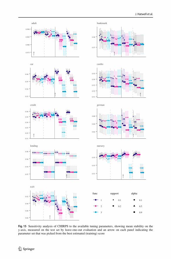
J. Hatwell et al.

1 3

Fig. 15 Sensitivity analysis of CHIRPS to the available tuning parameters, showing mean stability on the y-axis, measured on the test set by leave-one-out evaluation and an arrow on each panel indicating the parameter set that was picked from the best estimated (training) score


1 3

search as described in Sect. 7.5. The results are visualised in Fig. 15. The points show the mean stability scores on unseen data, along with standard error bars. Note, in the leg-end “func” indicates the score function configuration: (1) Support, � (snippet length) and Weights, (2) � and Weights, (3) Weights only. The left half of each panel contains the KL-div weighted scores, while the right half is unweighted scores. The binning (discretisation) function is set to 4 in the left quadrant of each half panel, and 8 on the right. In each panel, an arrow indicates the parameter set that gave the top mean rank on the training data, i.e., the final score after merging and pruning. This would suggest that the training scores alone provide an excellent predictor of the best parameter settings. There was no “universal” parameter set that did well on all data sets, however, the following general advice applies:

• A round of parameter tuning prior to implementation is very likely to yield improved performance in production, possibly increasing stability measures by a few percentage points.

• Lower support always yields better training scores for precision and stability. However, decreasing the support results in increasing the computation time per instance. The best trade off between these two variables will be a problem specific choice.

• The DKL weighting usually reduces the variance of the results. Varying the score func-tion does not usually have a significant effect when this weighting is set.

• However, in a few cases, greater stability is achievable with neutral weights. This set-ting should be investigated for critical problems where very small improvements are still significant.

• Discretisation settings make no difference for data sets that contain only categorical variables.

9 Conclusions and future work

We have expounded the rapidly developing research area of eXplainable Artificial Intel-ligence (XAI) and the need to interpret and explain black box models. Furthermore, we have made a case for relaxing the requirement to be model-agnostic; typically, a model and training data are “owned” by an actor or organisation wishing to adopt predictive analyt-ics. In these cases, decompositional methods that unpack the internal representation of a model are viable alternatives, especially if they outperform the model-agnostic approach. At the same time we have set out the need for additional requirements that have not been addressed in previous research. For example, concretely addressing the tendency to over- and under-fit, and providing a format for counter-factual information. From this foundation, we have proposed a novel formulation for explanations of black box classifiers on tabular data sets and an optimisation framework, including novel objective functions (stability and exclusive coverage) to generate better solutions.

The major contribution of this paper is the novel method, CHIRPS, for returning rule-based local explanations from Random Forests. Our experimental study shows that this method outperforms both local, model-agnostic methods, and globally interpretable meth-ods. CHIRPS is able to discover classification rules that are extremely precise, yet sur-prisingly general on a variety of data sets. The classification rules are enhanced with rich information about the contrastive, counter-factual cases, providing additional intuition for the end user.

J. Hatwell et al.

1 3

Our experimental study revealed scalability issues in competing methods. Over-coming these issues required prior restrictions such as reducing the number of trees by orders of magnitude, the maximum tree depths to little more than decision stumps, or setting the maximum cardinality of rules considered, thereby limiting higher order inter-actions. These settings place arbitrary limits on the solution space and put a distance between the model under scrutiny (the model to be explained) and the proxy model comprising the explanations themselves. We suggest that classification-rule-based explanation methods have many advantages over additive feature attribution methods (e.g. easy applicability to other instances) but to make some of the classification-rule-based methods truly scalable, there are open challenges for algorithmic optimisation.

Directions for future work are adapting CHIRPS to boosting classifiers, and vari-ants of the RF algorithm that use unbiased alternatives to CART. Replacing the simple greedy algorithm with modern multi-objective optimisation methods (e.g. genetic algo-rithms) is another avenue of research.

Open Access This article is licensed under a Creative Commons Attribution 4.0 International License, which permits use, sharing, adaptation, distribution and reproduction in any medium or format, as long as you give appropriate credit to the original author(s) and the source, provide a link to the Creative Com-mons licence, and indicate if changes were made. The images or other third party material in this article are included in the article’s Creative Commons licence, unless indicated otherwise in a credit line to the material. If material is not included in the article’s Creative Commons licence and your intended use is not permitted by statutory regulation or exceeds the permitted use, you will need to obtain permission directly from the copyright holder. To view a copy of this licence, visit http://creat iveco mmons .org/licen ses/by/4.0/.

Appendix

See Tables 15, 16, 17, and 18.

Table 15 Each explanation was generated from one held out instance and the precision measured on the remaining held out data

The mean ± standard errors are shown. The winning scores are printed in bold face

Anchors BRL CHIRPS defragTrees inTrees

adult 0.9530 ± 0.0052 0.7063 ± 0.0100 �.�� ± �.�� 0.8949 ± 0.0076 0.7628 ± 0.0092

bank 0.9457 ± 0.0052 0.4247 ± 0.0138 0.9838 ± 0.0017 �.�� ± �.�� 0.8754 ± 0.0079

car 0.9575 ± 0.0089 0.7904 ± 0.0139 �.�� ± �.�� 0.5837 ± 0.0168 0.9638 ± 0.0048

cardio 0.9419 ± 0.0085 0.5971 ± 0.0122 �.�� ± �.�� 0.7031 ± 0.0143 0.8196 ± 0.0104

credit 0.9805 ± 0.0084 0.5988 ± 0.0188 �.�� ± �.�� 0.5225 ± 0.0152 0.7226 ± 0.0203

german 0.8373 ± 0.0207 0.6250 ± 0.0190 �.�� ± �.�� 0.6341 ± 0.0186 0.6557 ± 0.0162

lending 0.9732 ± 0.0063 N/A �.�� ± �.�� 0.7259 ± 0.0124 N/Anursery 0.9662 ± 0.0055 0.8759 ± 0.0091 �.�� ± �.�� 0.5693 ± 0.0124 0.8259 ± 0.0084

rcdv 0.8332 ± 0.0097 0.2100 ± 0.0093 �.�� ± �.�� 0.7484 ± 0.0095 0.5436 ± 0.0082

http://creativecommons.org/licenses/by/4.0/


1 3

Table 16 Each explanation was generated from one held out instance and the stability measured on the remaining held out data

The mean ± standard errors are shown. The winning scores are printed in bold face


adult 0.9253 ± 0.0045 0.6677 ± 0.0090 �.�� ± �.�� 0.8946 ± 0.0076 0.7625 ± 0.0092

bank 0.9495 ± 0.0093 0.5801 ± 0.0093 0.9819 ± 0.0018 �.�� ± �.�� 0.8750 ± 0.0079

car 0.8806 ± 0.0075 0.7674 ± 0.0134 �.�� ± �.�� 0.5779 ± 0.0166 0.9356 ± 0.0047

cardio 0.8626 ± 0.0072 0.5871 ± 0.0111 �.�� ± �.�� 0.6867 ± 0.0140 0.7999 ± 0.0103

credit 0.9405 ± 0.0070 0.5853 ± 0.0179 �.�� ± �.�� 0.5006 ± 0.0135 0.6858 ± 0.0192

german 0.7926 ± 0.0133 0.6164 ± 0.0186 �.�� ± �.�� 0.6305 ± 0.0185 0.6132 ± 0.0150

lending 0.9347 ± 0.0051 N/A �.�� ± �.�� 0.7203 ± 0.0123 N/Anursery 0.8777 ± 0.0062 0.8494 ± 0.0089 �.�� ± �.�� 0.5674 ± 0.0123 0.8206 ± 0.0084

rcdv 0.7926 ± 0.0066 0.3913 ± 0.0062 �.�� ± �.�� 0.7465 ± 0.0095 0.5430 ± 0.0082

Table 17 Each explanation was generated from one held out instance and the coverage measured on the remaining held out data

This was repeated for entire held out data, or one thousand instances (whichever was the smaller). The mean ± standard errors are shown


adult 0.1613 ± 0.0047 0.2022 ± 0.0101 0.2506 ± 0.0050 0.4149 ± 0.0052 0.3823 ± 0.0048

bank 0.2918 ± 0.0056 0.4586 ± 0.0157 0.5272 ± 0.0055 0.2609 ± 0.0032 0.3444 ± 0.0042

car 0.2036 ± 0.0071 0.3843 ± 0.0148 0.2320 ± 0.0058 0.3584 ± 0.0039 0.1878 ± 0.0036

cardio 0.0866 ± 0.0030 0.6890 ± 0.0188 0.4256 ± 0.0082 0.1963 ± 0.0021 0.2685 ± 0.0062

credit 0.3212 ± 0.0099 0.6079 ± 0.0252 0.3180 ± 0.0076 0.8159 ± 0.0172 0.1789 ± 0.0055

german 0.1568 ± 0.0092 0.6579 ± 0.0213 0.1584 ± 0.0049 1.0000 ± 0.0000 0.1154 ± 0.0049

lending 0.1764 ± 0.0042 N/A 0.5380 ± 0.0087 0.5380 ± 0.0059 N/Anursery 0.1303 ± 0.0049 0.1502 ± 0.0059 0.1409 ± 0.0046 0.2742 ± 0.0021 0.2798 ± 0.0028

rcdv 0.0237 ± 0.0009 0.3480 ± 0.0151 0.0368 ± 0.0012 0.2173 ± 0.0038 0.2631 ± 0.0023

Table 18 Each explanation was generated from one held out instance and the exclusive coverage measured on the remaining held out data

This was repeated for entire held out data, or one thousand instances (whichever was the smaller). The mean ± standard errors are shown


adult 0.1556 ± 0.0045 0.0618 ± 0.0025 0.2457 ± 0.0048 0.3873 ± 0.0049 0.3196 ± 0.0051

bank 0.2387 ± 0.0033 0.0006 ± 0.0001 0.4969 ± 0.0048 0.2609 ± 0.0032 0.3106 ± 0.0039

car 0.2028 ± 0.0071 0.1720 ± 0.0060 0.2306 ± 0.0057 0.2409 ± 0.0026 0.1860 ± 0.0035

cardio 0.0851 ± 0.0029 0.0097 ± 0.0007 0.4098 ± 0.0078 0.1777 ± 0.0023 0.1777 ± 0.0023

credit 0.3177 ± 0.0098 0.1342 ± 0.0087 0.3138 ± 0.0075 0.0979 ± 0.0053 0.1688 ± 0.0050

german 0.1534 ± 0.0090 0.1099 ± 0.0069 0.1546 ± 0.0048 0.0000 ± 0.0000 0.1031 ± 0.0039

lending 0.1757 ± 0.0042 N/A 0.5215 ± 0.0082 0.2789 ± 0.0045 N/Anursery 0.1302 ± 0.0049 0.1332 ± 0.0048 0.1487 ± 0.0046 0.2492 ± 0.0023 0.2675 ± 0.0027

rcdv 0.0233 ± 0.0009 0.0001 ± 0.0000 0.0363 ± 0.0012 0.1623 ± 0.0023 0.1967 ± 0.0016

J. Hatwell et al.

1 3

References

Adnan MN, Islam MZ (2017) ForEx++: a new framework for knowledge discovery from decision forests. Australas J Inf Syst 21

Agrawal R, Srikant R et al (1994) Fast algorithms for mining association rules. In: Proceedings of 20th internatinal conference very large data bases, VLDB, vol 1215, pp 487–99

Andrews R, Diederich J, Tickle AB (1995) Survey and critique of techniques for extracting rules from trained artificial neural networks. Knowl-Based Syst 8(6):373–389

Biau G (2012) Analysis of a random forests model. J Mach Learn Res 13:1063–1095Bibal A, Frenay B (2016) Interpretability of machine learning models and representations: an introduction. In:

Michel V (ed) ESANN, computational intelligence and machine learning. Bruges, Belgium, pp 77–82Breiman L (2001) Random forests. Mach Learn 45(1):5–32Burrell J (2016) How the machine thinks: understanding opacity in machine learning algorithms. In: Big data

and society 3.1Clark P, Boswell R (1991) Rule induction with CN2: some recent improvements. In: Machine learning. Lecture

Notes in Computer Science 482 , pp 151–163Demsar J (2006) Statistical comparisons of classifiers over multiple data sets. J Mach Learn Res, pp 1–30Deng H (2014) Interpreting tree ensembles with intrees. Int J Data Sci Anal 7(4):277–87Dheeru D, Taniskidou EK (2017) UCI machine learning repository. University of California, Irvine, School of

Information and Computer Sciences, https ://archi ve.ics.uci.edu/ml/ datas ets/DoD Modeling and Simulation (M&S) Glossary (1998) Tech. rep. DoD 5000.59-M. Department of Defense,

Washington, p 124. https ://apps.dtic.mil/dtic/tr/fullt ext/u2/a3498 00.pdfDoshi-Velez F, Kim B (2017) Towards a rigorous science of interpretable machine learning. arXivpreprint

arXiv :1702.08608 European Parliament and Council of the European Union (2018) Regulation (EU) 2016/679 of the European

Parliament and of the Council of 27 April 2016 on the protection of natural persons with regard to the processing of personal data and on the free movement of such data, and repealing Directive 95/46/EC (General Data Protection Regulation)

Fen H et al (2019) Why should you trust my interpretation? Understanding uncertainty in LIME predictions. arXiv :1904.12991

Fernandez-Delgado M et al (2014) Do we need hundreds of classifiers to solve real world classification prob-lems. J Mach Learn Res 15(1):3133–3181

Freitas AA (2014) Comprehensible classification models: a position paper. ACM SIGKDD Explor Newsl 15(1):1–10

Friedman J , Popescu BE (2008) Predictive learning via rule ensembles. In: The annals of applied statistics 2.3 , pp 916–954

Friedman J (2001) Greedy function approximation: a gradient boosting machine. Ann Stat 29(5):1189–1232Garcia S et al (2009) A study of statistical techniques and performance measures for genetics-based machine

learning: accuracy and interpretability. In: Soft Computing 13.10 (Aug. 2009), pp 959–977Goodman B, Flaxman S (2016) European Union regulations on algorithmic decision-making and a right to

explanation. arXiv preprint arXiv :1606.08813 Guidotti R et al (2018) Local rule-based explanations of black box decision systems. arXiv :1805.10820 Gunning D (2017) Explainable artificial intelligence (XAI). In: Defense advanced research projects agency

(DARPA)Hand DJ (2006) Classifier technology and the illusion of progress. Stat Sci 21(1):1–14Hara S, Hayashi K (2016) Making tree ensembles interpretable: a Bayesian model selection approach. arXiv

:1606.09066 [stat]Hempel CG, Oppenheim P (1948) Studies in the logic of explanation. Philos Sci 15(2):135–175Hildebrandt M (2012) The dawn of a critical transparency right for the profiling era. Digital Enlight Yearb

2012:41–56Ho TK, Basu M (2002) Complexity measures of supervised classification problems. IEEE Trans Pattern Anal

Mach Intell 24(3):289–300Huysmans J, Baesens B, Vanthienen J (2006) Using rule extraction to improve the com-prehensibility of predic-

tive models. SSRN Electron J. https ://tinyu rl.com/ y79jk 4xx (visited on 11/16/2018)Ishwaran H (2007) Variable importance in binary regression trees and forests. Electron J Stat 1:519–537Jovanovic M et al (2016) Building interpretable predictive models for pediatric hospital readmission using Tree-

Lasso logistic regression. In: Artificial intelligence in medicine 72(Sept. 2016), 1221Lakkaraju H, Bach SH, Leskovec J (2016) Interpretable decision sets: a joint framework for description and

prediction. In: Proceedings of the 22nd ACM SIGKDD international conference on knowledge discovery and data mining—KDD ’16. ACM Press, San Francisco, pp 1675–1684

https://archive.ics.uci.edu/ml/%20datasets/

https://apps.dtic.mil/dtic/tr/fulltext/u2/a349800.pdf

http://arxiv.org/abs/1702.08608






https://tinyurl.com/%20y79jk4xx


1 3

Letham B (2015) Statistical learning for decision making: interpretability, uncertainty, and inference. Ph.D. the-sis. Massachusetts Institute of Technology

Letham B et al (2015) Interpretable classifiers using rules and Bayesian analysis: building a better stroke predic-tion model. Ann Appl Stat 9(3):1350–1371

Lipton ZC (2016) The mythos of model interpretability. arXiv preprint arXiv :1606.03490 Louppe G (2014) Understanding random forests: from theory to practice. Ph.D. thesis. Universite de Liege,

LiegeLundberg SM, Erion GG, Lee S-I (2017) Consistent individualized feature attribution for tree ensembles. arXiv

:1802.03888 [cs, stat]. Sydney, AustraliaLundberg SM, Lee S-I (2017) A unified approach to interpreting model predictions. In: Advances in neural

information processing systems, pp 4768–4777Malioutov DM , Varshney KR (2013) Exact rule learning via boolean compressed sensing. In: ICML, pp

765–773Mashayekhi M , Gras R (2015) Rule extraction from random forest: the RF+HC methods. In: Advances in

artificial intelligence 2015. Vol. 9091. Lecture notes in computer science Artificial intelligence. Springer, Halifax, pp 223–237

Michal F (2019) Please, explain. Interpretability of black-box machine learning models.https ://tinyu rl.com/y5qru qgf (visited on 04/19/2019)

Miller T (2017) Explanation in artificial intelligence: insights from the social sciences. arXiv preprint arXiv :1706.07269

O’Neil T, Hayworth C (2018) Today (excerpt), BBC Radio 4Paluszynska A (2017) Structure mining and knowledge extraction from random forest with applications to the

Cancer Genome Atlas project. Ph.D. thesis. University of WarsawPasquale F (2015) The black box society: the secret algorithms that control money and information. Harvard

University Press, CambridgePei J, Han J (2000) Mining frequent patterns without candidate generation. In: Proceedings of conference on the

management of data. ACM Press, DallasProenca HM, van Leeuwen M (2019) Interpretable multiclass classification by MDL-based rule lists. arXiv

:1905.00328 Quinlan JR (1987) Generating production rules from decision trees. In: Proceedings of the tenth international

joint conference on artificial intelligence. Milan, Italy, pp 304–307Ribeiro MT, Singh S, Guestrin C (2016) Why should I trust you?: explaining the predictions of any classifier.

ACM Press, pp 1135–1144Ribeiro MT, Singh S, Guestrin C (2018) Anchors: high-precision model-agnostic explanations. In: Conference

on artificial intelligence, 2018. New OrleansRiiping S (2006) Learning interpretable models. Ph.D. thesis. Dortmund: der Universitat DortmundRudin C (2018) Please stop explaining blackbox models for high stakes decisions. arXiv :1811.10154 [cs, stat]Salmon W (1971) Statistical explanation and statistical relevance. University of Pittsburgh Press, PittsburghSouillard-Mandar W et al (2016) Interpretable machine learning models for the digital clock drawing test. In:

arXivpreprint arXiv : 1606.07163 Subianto M, Siebes A (2007) Understanding discrete classifiers with a case study in gene prediction. In: IEEE,

pp 661–666Tibshirani R (1996) Regression shrinkage and selection via the lasso. J R Stat Soc 58(1):267–288Tierney D (2017) The morality of artificial intelligenceTurgeman L, May JH (2016) A mixed-ensemble model for hospital readmission. In: Artificial intelligence in

medicine 72 (Sept. 2016), 72–82Vapnik VN (1998) Statistical learning theory. Adaptive and learning systems for signal processing, communica-

tions, and control. Wiley, New YorkVens C, Costa F (2011) Random Forest based feature induction. In: IEEE, pp 744–753Waitman LR, Fisher DH, King PH (2006) Bootstrapping rule induction to achieve rule stability and reduction. J

Intell Inf Syst 27(1):49–77Wang T et al (2015) Or’s of and’s for interpretable classification, with application to context-aware recom-

mender systems. arXiv :1504.07614 Wang T et al (2016) Bayesian rule sets for interpretable classification. In: Data mining (ICDM), 2016 IEEE

16th international conference on. IEEE, pp 1269–1274Wang T et al (2017) A Bayesian framework for learning rule sets for interpretable classification. J Mach Learn

Res 18:37Wang F, Rudin C (2015) Falling rule lists. In: Proceedings of the 18th international conference on artificial

intelligence and statistics. vol 38. San Diego, pp 1013–1022Wilkinson S (2014) Levels and kinds of explanation: lessons from neuropsychiatry. In: Frontiers in psychology, 5




https://tinyurl.com/y5qruqgf

https://tinyurl.com/y5qruqgf








J. Hatwell et al.

1 3

Woodward J (2017) Scientific explanation.https ://tinyu rl.com/ydg95 j85 (visited on 08/08/2018)Yang HY, Rudin C, Seltzer M (2017) Scalable Bayesian rule lists. In: Proceedings of the 34th international

conference on machine learning

Publisher’s Note Springer Nature remains neutral with regard to jurisdictional claims in published maps and institutional affiliations.

https://tinyurl.com/ydg95j85

CHIRPS: Explaining random forest classification

Documents

Transcript of CHIRPS: Explaining random forest classification