Josephine van Eggelen

Explaining phenotypical variation by assessing genetic variation in Brassica

oleracea.

Preforming a genome wide association study in a highly admixture Brassica oleracea population

Examiners:dr. ir. A.B. Bonnemadr. C.W.B. Bachem

MSc. Thesis Plant SciencesPlant Breeding and Genetic ResourcesWageningen University

iii

MSc thesis Plant Breeding Wageningen University

Student: Josephine van Eggelen Contact details: josephine.vaneggelen@wur.nl Student number: 920316217080 Study program: MSc Plant Science WUR department: Plant Breeding Department, Growth and development group Supervisor: dr.ir. A.B. Bonnema guusje.bonnema@wur.nl Second Supervisor: dr. Christian Bachem christian.bachem@wur.nl ECTs: 36 Start Date: 01-05-2017 End Date: 02-11-2017

“Copyright © 2016 All rights reserved. No part of this document may be reproduced or distributed in any form by any means, without the prior consent of the author.”

iv

Abstract

Brassica oleracea is, with all the diverse morphotypes, an economical important and health promoting plant family, of which currently insufficient scientific information regarding the genetic variation available is. The aim of the thesis is defined as explaining phenotypical variation in leaf development by assessing genetic variation in Brassica oleracea by preforming a GWAS.

Phenotypic variation is scored, on a highly diverse collection of B. oleracea of 842 accessions, consisting of eleven morphotypes of gene banks accessions (502) as well as hybrids (340). Leaf traits are scored by detaching developed leaves and analyzing those using Halcon. However, developing a script is difficult since the variety in leaf morphology is tremendously high. Data retrieved by Halcon was not accurate enough to be used in this study, so only traits scored manually, leaf blistering and cabbage head weight are used. Genotypic variation was gathered on two levels, a whole genome sequence study was conducted on 123 accessions, and sequence based genotype data, which consist of 18,580 markers semi-equally distributed over the genome.

Population structure is calculated to establish a method to correct GWAS, in this study the population structure five k-groups. The number of significant marker found in GWAS for head weight is 19, whereas 822 are associated to leaf blistering. Candidate markers are selected based on a high LOD (-log10) score, >FDR threshold, interesting flanking regions, function and previous studies. The candidate markers are converted into a candidate region (50 kb both sides). In total, 45 candidate genes for leaf blistering and 47 for head weight are found. The candidate genes are then, subjected to a function analysis, in total, four candidate genes for blistering are found: TCP4, SPL3, ARF3 and OFP16. Additionally, eight candidate genes for head weight are found: IAA19, PME35, PAR2, PAP1, APUM19, TOE2, APPR3 and ZFP3. The candidate genes are then selected on a lack of paralogous and a unique restriction enzyme cutting site. OFP16 and restriction enzymes Acclll and BsiWl, and ZFP3 and the restriction enzyme Psil are found. Only when the PCR product of OFP16 was cut with the restriction enzyme BsiWI different bands could be detected. However, the results do not show a trend in extensive leaf blistering, for homozygous accessions. Therefore, further research to the candidate genes found in this study is recommended.

v

Table of Contents

Abstract ................................................................................................................................................... iv

Table of Contents ..................................................................................................................................... v

Definitions ............................................................................................................................................. viii

1 Introduction .......................................................................................................................................... 1

1.1 Research background .................................................................................................................... 1

1.2 Brassicaceae family ....................................................................................................................... 1

1.3 Brassica oleracea ........................................................................................................................... 2

1.4 Leaf development .......................................................................................................................... 3

1.5 Head formation ............................................................................................................................. 5

1.6 Candidate genes ............................................................................................................................ 6

1.7 Association mapping ..................................................................................................................... 7

2 Conceptual design ................................................................................................................................ 8

2.1 Aim................................................................................................................................................. 8

3 Technical research design .................................................................................................................... 9

3.1 Materials ........................................................................................................................................ 9

3.1.1 Plant material ......................................................................................................................... 9

3.1.2 Sequence data ...................................................................................................................... 10

3.2 Method ........................................................................................................................................ 10

3.2.1 Phenotypical data ................................................................................................................. 10

3.2.2 Genomic data ....................................................................................................................... 12

3.2.3 Statistical analysis ................................................................................................................. 13

3.2.4 Candidate gene ..................................................................................................................... 14

3.2.5 Validating candidate genes .................................................................................................. 14

4 Results ................................................................................................................................................ 15

4.1 Phenotypic results ....................................................................................................................... 15

4.1.1 Photo traits ........................................................................................................................... 15

4.1.2 Non-photo traits ................................................................................................................... 16

4.2 Genotypic results ......................................................................................................................... 17

4.2.1 Population structure ............................................................................................................. 17

4.2.2 Genome wide association study ........................................................................................... 19

4.3 Candidate markers ...................................................................................................................... 20

4.4 Candidate genes .......................................................................................................................... 21

5 Discussion ........................................................................................................................................... 26

5.1 Phenotypic ................................................................................................................................... 26

vi

5.1.1 Field trial ............................................................................................................................... 26

5.1.2 Photo traits ........................................................................................................................... 26

5.1.3 Non-photo traits ................................................................................................................... 27

5.2 Genotypic .................................................................................................................................... 27

5.2.1 Sequence data ...................................................................................................................... 27

5.2.2 Population structure ............................................................................................................. 28

5.2.3 Genome wide association mapping ..................................................................................... 28

5.3 Candidate gene ............................................................................................................................ 29

Conclusion & recommendation ............................................................................................................. 32

Acknowledgement ................................................................................................................................. 33

References ............................................................................................................................................. 34

Appendix ................................................................................................................................................ 38

Appendix I: Overview field ................................................................................................................ 38

Appendix II: Scored traits .................................................................................................................. 39

Appendix III: Karyotype Brassica genome ......................................................................................... 40

Appendix IV: Morphotypes tested .................................................................................................... 41

Appendix V: Protocols ....................................................................................................................... 42

Appendix VI: ANOVA ......................................................................................................................... 46

Appendix VII Q-Q plots ...................................................................................................................... 48

Appendix VIII: Candidate markers ..................................................................................................... 50

Appendix IX: Candidate genes ........................................................................................................... 54

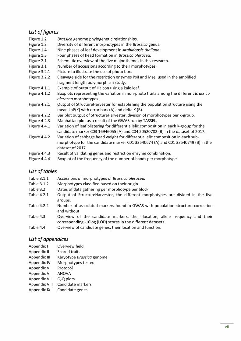
vii

List of figures Figure 1.2 Brassica genome phylogenetic relationships. Figure 1.3 Diversity of different morphotypes in the Brassica genus. Figure 1.4 Nine phases of leaf development in Arabidopsis thaliana. Figure 1.5 Four phases of head formation in Brassica oleracea. Figure 2.1 Schematic overview of the five major themes in this research. Figure 3.1 Number of accessions according to their morphotypes. Figure 3.2.1 Picture to illustrate the use of photo box. Figure 3.2.2 Cleavage side for the restriction enzymes PsiI and MseI used in the amplified

fragment length polymorphism study. Figure 4.1.1 Example of output of Halcon using a kale leaf. Figure 4.1.2 Boxplots representing the variation in non-photo traits among the different Brassica

oleracea morphotypes. Figure 4.2.1 Output of StructureHarvester for establishing the population structure using the

mean LnP(K) with error bars (A) and delta K (B). Figure 4.2.2 Bar plot output of StructureHarvester, division of morphotypes per k-group. Figure 4.2.3 Manhattan plot as a result of the GWAS run by TASSEL. Figure 4.4.1 Variation of leaf blistering for different allelic composition in each k-group for the

candidate marker C03 16946055 (A) and C04 20520782 (B) in the dataset of 2017. Figure 4.4.2 Variation of cabbage head weight for different allelic composition in each sub-

morphotype for the candidate marker C01 33540674 (A) and C01 33540749 (B) in the dataset of 2017.

Figure 4.4.3 Result of validating genes and restriction enzyme combination. Figure 4.4.4 Boxplot of the frequency of the number of bands per morphotype.

List of tables Table 3.1.1 Accessions of morphotypes of Brassica oleracea. Table 3.1.2 Morphotypes classified based on their origin. Table 3.2 Dates of data gathering per morphotype per block. Table 4.2.1 Output of StructureHarvester, the different morphotypes are divided in the five

groups. Table 4.2.2 Number of associated markers found in GWAS with population structure correction

and without. Table 4.3 Overview of the candidate markers, their location, allele frequency and their

corresponding -10log (LOD) scores in the different datasets. Table 4.4 Overview of candidate genes, their location and function.

List of appendices Appendix I Overview field Appendix II Scored traits Appendix III Karyotype Brassica genome Appendix IV Morphotypes tested Appendix V Protocol Appendix VI ANOVA Appendix VII Q-Q plots Appendix VIII Candidate markers Appendix IX Candidate genes

viii

Definitions

Concepts and definitions used throughout the report are defined in this section to ensure clarity. Morphotype: “Species that encompass highly diverse crops as a result of artificial selection during domestication and breeding, and display extreme morphological characteristics” (Cheng, Sun, et al., 2016). Morphotypes are often described as sub-species such as cauliflower ssp. botrytis and kale ssp. acephala.

Blistering: density of 'curving' on leaves at middle of the plant, examples are shown in Appendix II.

1

1 Introduction

This section presents the research background, it starts with emphasizing the importance of this research, in section 1.1. Followed by an introduction in the Brassicaceae family in section 1.2. An overview of the species Brassica oleracea (B. oleracea) is provided in section 1.3. Section 1.4 represents an introduction to leaf development and section 1.5 an introduction to head formation. Followed by candidate genes potentially useful in this research, detailed in section 1.6. Finally, an introduction in association mapping, a method crucial in this research is provided in section 1.7.

1.1 Research background In total there are 3709 genera in the Brassicaceae family (Warwick & Al-Shehbaz, 2006). The

Brassica genus comprises of a diverse group of important vegetable, oil-, fodder- and condiment crops (Artemyeva, Chesnokov, Vavilov, Budahn, & Bonnema, 2013). The Brassica genus provides vegetables which are an important source of nutrients, containing several health-promoting phytochemicals, for example, glucosinolates, phenolic acids and flavonoids (Avato & Argentieri, 2015). These components are known for their beneficial effects against certain diseases, such as reducing the risk of cancer.

Brassica species originated from a common ancestor about 15 million years ago. Domestication of Brassica begun around 500 years ago, resulting in the multiple diverse species that the genus represents now (J. Zhao et al., 2010). Cabbages and other brassicas (Chinese, mustard cabbage, pak choy (B. chinensis), including white, red, savoy cabbage, Brussels sprouts, collards, kale and kohlrabi (all brassica varieties except cauliflower)) are now cultivated in 152 countries in a total area of 2.4 million hectares (“FAOSTAT,” 2017). This demonstrates the economic importance of Brassicaceae family. Considering the nutritional and economical importance of the Brassica genus family genetic studies should focus on obtaining a broader understanding of the variability of the Brassicaceae family. Additionally, the origin and relationship among the genome of the species within the Brassicaceae family can be applied for efficiently breeding brassica crops (Li, Kitashiba, Inaba, & Nishio, 2009).

To conclude, the Brassicaceae family is an important crop family worldwide, many different varieties are present as the crop is adapted to different climates. The enormous variability leads to a genetically diverse and therefore interesting variation both within the morphotypes and between the different morphotypes. Therefore, this project is aimed to develop a case study to understand leaf development using the modern tools and comparative genomics. Understanding the variation within the Brassica genus can support future crop breeding for selection of genetic traits to optimize plant fitness.

1.2 Brassicaceae family Brassica is the most important genus in this research. Brassica and Arabidopsis are both genera

of the Brassicaceae family, making them analogous. Brassica and Arabidopsis diverged around 15 million years ago from a common ancestor (Figure 1.2) (Cheng et al., 2017). Brassicas evolved after a whole genome triplication (WGT) event from this Brassica ancestor (Figure 1.2) (Jingyin Yu et al., 2013). Now, six Brassica crop species form the ‘triangle of U’ model, comprising three diploid species — B. rapa (A genome; n=10), B. nigra (B genome; n=8) and B. oleracea (C genome; n=9) — and three allotetraploids resulting from pairwise hybridization between diploids — B. napus (AC genome; n=19), B. juncea (AB genome; n=18) and B. carinata (BC genome n=17) (Figure 1.2) (Cheng, Sun, et al., 2016); (Cheng, Wu, et al., 2016). Domestication and selection of these Brassicas has resulted in extreme morphotypes such as leafy heads, enlarged organs (e.g. roots, leaves, leaf buds, stems and inflorescences) and extensive axillary branching (Cheng, Wu, et al., 2016) (Figure 1.3).

2

Figure 1.2 Brassica genome phylogenetic relationships. Arabidopsis thaliana was used as outgroup, whereas Schrenkiella parvula was employed to indicate the point of whole genome triplication. The chromosome number per morphotypes is indicated as well. Modified from: Genome sequencing supports a multi-vertex model for Brassicaceae species (Cheng et al., 2017).

1.3 Brassica oleracea This research focusses merely on B. oleracea, as it is the most important genus of the

Brassicaceae family, considering the European vegetable market (“FAOSTAT,” 2017). Brassica oleracea consists of the following morphotypes: red, white, savoy and pointed cabbage, cauliflower, broccoli, tronchuda, kale, collard green, Chinese kale, kohlrabi and Brussels sprout (subset shown in Figure 1.3). The different morphotypes are self-incompatible.

The genome sequence of B. oleracea is available and consists of nine chromosomes, whereby 1,848 scaffold, with 45,758 predicted genes, 13,382 transposable elements and 3,581 non-coding RNAs are found (Liu et al., 2014; Parkin, 2005; Jingyin Yu et al., 2013). When comparing B. oleracea DNA to Arabidopsis thaliana (A. thaliana) DNA sequences, the two genera are 75-90% similar in exons and ≤70% in intron regions (Ayele et al., 2005).

Figure 1.3 Diversity of different morphotypes in the Brassica genus. Phylogenetic tree displaying seven distinctive

morphotypes of Brassica oleracea. Modified from figure 1 Subgenome parallel selection is associated with morphotype diversification and convergent crop domestication in Brassica rapa and Brassica oleracea (Cheng, Wu, et al., 2016)

3

1.4 Leaf development Key to a plants survival are well developed leaves considering trade-offs, simply said: leaf area

should be as large as possible, to absorb light energy and leaves should be as flat as possible to facilitate gas exchange (Tsukaya, 2005). To photosynthesize efficiently the shape and size of plant leaves are crucial. Control of leaf shape is therefore an important mechanism for a plants fitness and has been refined through the course of evolution (Tsukaya, 2005). Leaf shape is largely conserved between species, although mutations can result in different phenotypes (Kalve, De Vos, & Beemster, 2014).

Figure 1.4 represents the leaf development in A. thaliana, subdivided in nine phases to illustrate the leaf development process in plants. Kalve (2014) and colleagues reviewed current literature on regulatory mechanisms in leaf formation. As A. thaliana and B. oleracea belong to the same Brassicaceae family, studying known leaf development processes in A. thaliana will help to understand the leaf development process in B. oleracea. The development of leaves is a complex process involving multiple independent regulatory pathways (Kalve et al., 2014). Finally, the main differences in leaf morphology result from alterations in cell growth rates along the principal developmental axes (Kalve et al., 2014).

Figure 1.4 Nine phases of leaf development in Arabidopsis thaliana. The developmental path of cells is indicated

with red arrows; key regulatory processes are numbered and indicated. Modified from Figure 1 Leaf development: a

cellular perspective (Kalve et al., 2014).

First, a broad overview, based on the nine phases in leaf development (Figure 1.4) will be given, then the phases and potential genes involved in this process will be detailed. Leaf expansions is characterized by two major developmental processes: cell proliferation and cell expansion (Tsukaya, 2005). These two major development processes are sub-divided into the nine phases explained below. The first phase in leaf development is the stem cell maintenance in the shoot apical meristem (SAM) where stem cells (not) lose their stem cell identity. The second phase is leaf initiation where stem cells start to develop. The third phase is leaf-polarity control, where the cells develop into adaxial (upper)

4

and abaxial (lower) sides. Then, the development of the mature leaf starts with cytoplasmic growth (4), followed by cell division (5), endoreduplication (6), transition phase (7), cell expansion (8) and cell differentiation (9) (Kalve et al., 2014).

1. Stem cell maintenance in SAM; SAM is the birthplace of all cells, cells will differentiate from stem cells into leaves, axillary nodes and floral parts. When stem cells drift from the quiescent center, where they originate from, they lose the stem cell fate and reach the dividing state (Kalve et al., 2014). This phase is controlled by the transcription factor WUSCHEL (WUS) and the CLAVATA gene products (CLV1, CLV2 and CLV3) (Carles & Fletcher, 2003). WUS induces the production of non-cell autonomous signal that regulates mediated stem cell maintenance by inhibition of the F-box protein LEAF CURLING RESPONSIVENESS (LCR). Firstly, WUS activates CLV3, which then binds to CLV1 and CLV2 to eventually inhibit WUS activity (Carles & Fletcher, 2003; Kalve et al., 2014). Furthermore, cytokinin (CK) a plant hormone, effects the WUS activity by CLV-dependent and CLV-independent mechanisms (Gordon, Chickarmane, Ohno, & Meyerowitz, 2009; Kalve et al., 2014).

2. Leaf initiation; when a cell is converted to a non-stem cell, the cell has the choice between staying in the main axis or differentiate. This process is regulated by the plant hormone auxin and it’s influx carrier AUXIN RESISTANT (AUX1) and it’s efflux carrier PIN-FORMED (PIN1) (Bayer et al., 2009; Kalve et al., 2014). KNOTTED-like homeobox (KNOX1) and ASYMMETRIC LEAF1 / ROUGH SHEATH2 / PHANTASTIC (ARP) are two antagonistic transcription factors playing an important role in the distinction of cells. KNOX is expressed in the meristem cells to maintain undifferentiated cells in SAM; the KNOX gene BREVIPENDICELLUS (BP) regulates leaf initiation. In contrast to ARP, regulates the emergence of a primordium (Kalve et al., 2014; Scofield & Murray, 2006).

3. Leaf polarity control; when the leaf primordium is established, the primordium develops a polarity gradient (Kalve et al., 2014). The adaxial domain can be identified by the expression of PHABULOSA (PHB), PHAVOLUTA (PHV) and REVOLUTA (REV) genes (McConnell et al., 2001). Whereas the abaxial domain can be identified by the expression of KANADI (KAN) and the YABBY gene family (Bowman, Eshed, & Baum, 2002; Kalve et al., 2014). Additionally, the Auxin Response Factor (ARF) gene is also regulated by a gene from the YABBY family resulting in a positive feedback loop regarding the abaxial domain. Furthermore, ANGUSTIFOLIA (AN), regulates the polar expansion in the lateral (leaf width) direction and ROTUNDIFOLIA3 (ROT3) in the longitudinal (leaf-length) direction (Tsukaya, 2005). Additionally, several over these genes are severely regulated by miRNA’s such as miRNA165/166, that target the degradation of ARF on the abaxial side.

4. Cytoplasmic growth; the Target Of Rapamycin (TOR) pathway plays an important role in cytoplasmic growth. TOR controls the cytoplasmic growth in a cell by, positively controlling ribosome biogenesis, cell cycle, translational initiation cell proliferation and cell expansion. Conversely, TOR inhibits autophagy and accumulation of carbon resources (Kalve et al., 2014; Zhang, Persson, & Giavalisco, 2013). Important genes in cell wall formation are expansins (EXPs) which confirm the TOR-pathway playing a role in cell expansion.

5. Cell division; the cell cycle of the plant is largely controlled by two cyclin-dependent kinases; A-type cyclin dependent kinases (CDKA) and D-type cyclin (CYCD). Both are important in the DNA duplication phase (Gaamouche et al., 2010; Kalve et al., 2014). Auxin, CK, gibberellin and brassinosteroid upregulate CYCD and thereby activate CDKA.

6. Endoreduplication; “Endoreduplication is the process whereby DNA replicates repeatedly, without alternating divisions through mitosis, causing a high ploidy level in the cell” (Kalve et al., 2014). For endoreduplication to occur, the CDK activity must be limited (de Veylder, Larkin, & Schnittger, 2011; Kalve et al., 2014). Kip Related Proteins (KRP), SIAMESE (SIM) family proteins and SIAMESE Related (SMR) family proteins inhibit CDK activity (Kalve et al., 2014; J. D. Walker, Oppenheimer, Concienne, & Larkin, 2000).

5

7. Transition phase; auxin, plays an important role in the transition from cell proliferation to cell expansion. Auxin induces the expression of the following gene: AUXIN REGULATED GENE INVOLVED IN ORGAN SIZE (ARGOS) (Hu, Xie, & Chua, 2003). Overexpression of ARGOS results in an increase in leaf size whereas downregulation of ARGOS results in a decrease of leaf size. ARGOS plays an important role in cell proliferation as well, it positively regulates the protein AINTEGUMENTA (ANT) that is a DNA-binding protein, in order to promote cell division (Hu et al., 2003). Similar to the ANT proteins, the transcription factors GROWTH REGULATING FACTOR (GRF) and TEOSINTE BRANCHED/CYCLOIDEA/PCF (TCP) promote cell division. Whereby, miRNA319 blocks the transcription factor TCP. Furthermore, the gene ORGAN SIZE RELATED1 (ORS1) positively regulates cell division and expansion (Hu et al., 2003).

8. Cell expansion; Cell expansion occurs when; the cell walls loosen, so water can be taken up. Cell walls can extend due to change in turgor pressure, then, cell walls stiffen again and accumulate the cell wall compartments (Wolf, Hématy, & Höfte, 2012). Unfortunately, the molecular pathway of this process is not known. Although it is known that auxin and brassinolida are actively involved with the P-type plasma membrane proton ATPase (AHA), that activates loosening of the cell wall by EXP proteins and xyloglucanendotransglucosylase / hydrolases (XTH), xyloglucan endohydrolase (XEH) and xyloglucan endotransglucosylase (XET) (Wolf et al., 2012). Furthermore, the TOR pathway is directly involved in cell expansion by aligning several genes to glucose signaling to positively affect the nutrient status (Kalve et al., 2014; Xiong et al., 2014).

9. Cell differentiation; finally, cells will differentiate into distinctive cell types, for example, guard cells, vascular tissue cells, and trichomes. Differentiation in the different cell types involves different pathways involving different molecular mechanisms (Kalve et al., 2014).

1.5 Head formation Cabbages (red, white, savoy, pointed) are head-forming crops, making them important leafy

vegetables. Scientific literature concerning head formation in B. oleracea is limited, head formation in B. rapa is studied to some extend and discussed here.

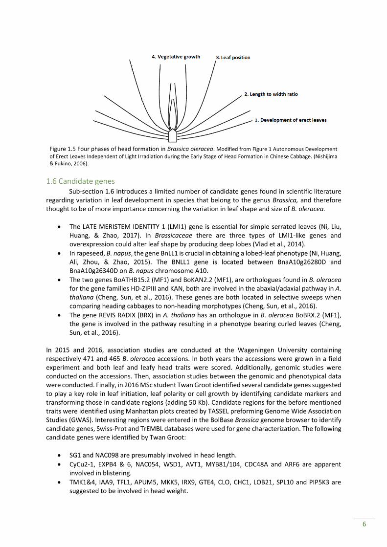
Heads are formed as a result of the blanching from self-shading according to (Nishijima & Fukino, 2006). Head formation depends on two morphological traits: 1) the development of erect leaves; 2) round-shaped leafs lacking a petiole, causing the leaf to have a low length to width ratio (Nishijima & Fukino, 2006). These factors lead to overlapping leaves that induce head formation.

Tanaka and colleagues investigated early maturing cabbage varieties. The results show that early maturing hybrids develop the following characteristics: increase in leaf shape index (width/length) of wrapper leaves and the leaf position at which head formation started (Tanaka & Niikura, 2003). First, when a plant starts to grow the number of wrapper leaves increase. Secondly, the leaf shape index of the wrapper leaves increases. Thirdly, the head is formed, head formation in hybrids occurs when wrapper leaf change to a high ratio leaf shape index from a low leaf position. Fourth and final, the head reaches maturity by increasing the number and weight of the head leaves during continuous vegetative growth (Tanaka & Niikura, 2003). All phases are summarized in Figure 1.5.

6

Figure 1.5 Four phases of head formation in Brassica oleracea. Modified from Figure 1 Autonomous Development

of Erect Leaves Independent of Light Irradiation during the Early Stage of Head Formation in Chinese Cabbage. (Nishijima & Fukino, 2006).

1.6 Candidate genes Sub-section 1.6 introduces a limited number of candidate genes found in scientific literature regarding variation in leaf development in species that belong to the genus Brassica, and therefore thought to be of more importance concerning the variation in leaf shape and size of B. oleracea.

The LATE MERISTEM IDENTITY 1 (LMI1) gene is essential for simple serrated leaves (Ni, Liu, Huang, & Zhao, 2017). In Brassicaceae there are three types of LMI1-like genes and overexpression could alter leaf shape by producing deep lobes (Vlad et al., 2014).

In rapeseed, B. napus, the gene BnLL1 is crucial in obtaining a lobed-leaf phenotype (Ni, Huang, Ali, Zhou, & Zhao, 2015). The BNLL1 gene is located between BnaA10g26280D and BnaA10g26340D on B. napus chromosome A10.

The two genes BoATHB15.2 (MF1) and BoKAN2.2 (MF1), are orthologues found in B. oleracea for the gene families HD-ZIPIII and KAN, both are involved in the abaxial/adaxial pathway in A. thaliana (Cheng, Sun, et al., 2016). These genes are both located in selective sweeps when comparing heading cabbages to non-heading morphotypes (Cheng, Sun, et al., 2016).

The gene REVIS RADIX (BRX) in A. thaliana has an orthologue in B. oleracea BoBRX.2 (MF1), the gene is involved in the pathway resulting in a phenotype bearing curled leaves (Cheng, Sun, et al., 2016).

In 2015 and 2016, association studies are conducted at the Wageningen University containing respectively 471 and 465 B. oleracea accessions. In both years the accessions were grown in a field experiment and both leaf and leafy head traits were scored. Additionally, genomic studies were conducted on the accessions. Then, association studies between the genomic and phenotypical data were conducted. Finally, in 2016 MSc student Twan Groot identified several candidate genes suggested to play a key role in leaf initiation, leaf polarity or cell growth by identifying candidate markers and transforming those in candidate regions (adding 50 Kb). Candidate regions for the before mentioned traits were identified using Manhattan plots created by TASSEL preforming Genome Wide Association Studies (GWAS). Interesting regions were entered in the BolBase Brassica genome browser to identify candidate genes, Swiss-Prot and TrEMBL databases were used for gene characterization. The following candidate genes were identified by Twan Groot:

SG1 and NAC098 are presumably involved in head length.

CyCu2-1, EXPB4 & 6, NAC054, WSD1, AVT1, MYB81/104, CDC48A and ARF6 are apparent involved in blistering.

TMK1&4, IAA9, TFL1, APUM5, MKK5, IRX9, GTE4, CLO, CHC1, LOB21, SPL10 and PIP5K3 are suggested to be involved in head weight.

7

1.7 Association mapping Genome Wide Association Study (GWAS) is used to explore the genetic diversity in a large

collection of genotypes. GWAS is used to identify loci for which an allelic polymorphisms is potentially associated with the phenotypic variation (Artemyeva et al., 2013). Therefore, GWAS tests the association of molecular markers with variation in traits of interest, in populations making use of linkage disequilibrium (LD). Linkage disequilibrium is the nonrandom association of alleles at different loci in both natural and breeding populations (Artemyeva et al., 2013).

Association studies with high density SNP coverage, large sample size and minimum population structure are useful in dissecting complex traits, such as leaf development and head formation (Zhu, Gore, Buckler, & Yu, 2008). Genome wide association study is used because compared with QTL, more variation can be observed in designed bi-parental segregating populations (J. Zhao et al., 2010). Genome wide association study and QTL mapping differs in, that association mapping makes use of the natural genetic variation and the historical recombination found in the mapping population (Zhu et al., 2008). Furthermore, the mapping resolution is higher in GWAS compared with that in populations from controlled crosses. However, disadvantages of association mapping is that subpopulations might be present, the usage of LD is controversial since LD can occur because of multiple reasons such as genetic drift and selection (J. Zhao et al., 2010).

8

2 Conceptual design

This chapter introduces the aim of the research that is conducted. Section 2.1 emphasizes the importance of the research, the research objective, aim and the five major themes of the research, are presented.

2.1 Aim Brassica oleracea is, with all the diverse morphotypes, an economical important and health

promoting plant family. At this moment, sufficient scientific information on the genetics behind leaf and head development in B. oleracea is lacking. Therefore, the initial aim of the research was to obtain insight in the genetic variation of the B. oleracea species regarding leaf and head morphology and development, in a highly diverse collection. This aim would be reached by studying phenotypical variation of leaf traits and explaining those differences on a genomic level. However, due to time limitations and inadequate research methods, results were not sufficient and not validated. Therefore, we were not able to draw the conclusions we hoped to draw. Hence, this thesis project is set as a case study, describing two verified leading examples. Whereby the aim of the thesis is defined as:

Explaining phenotypical variation in leaf development by assessing genetic variation in Brassica oleracea.

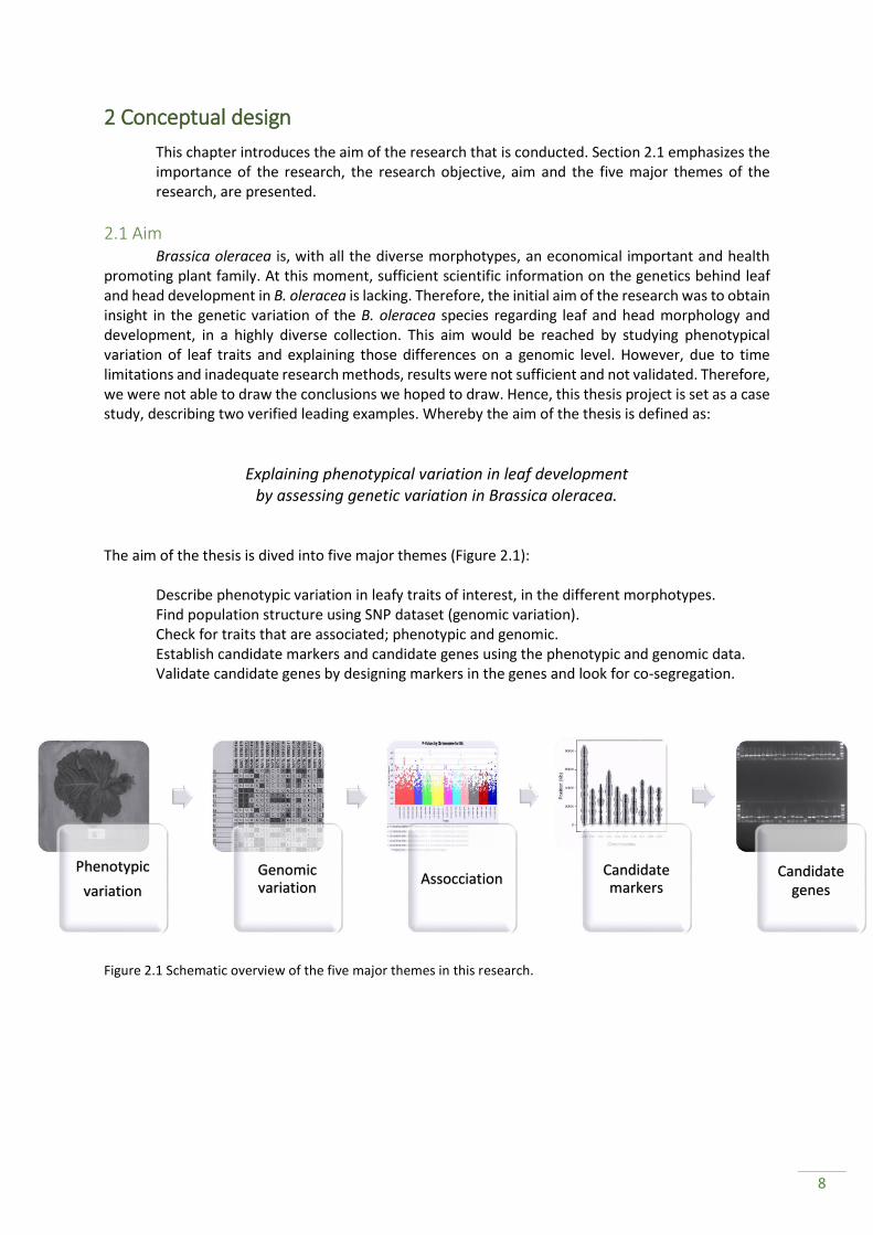
The aim of the thesis is dived into five major themes (Figure 2.1):

Describe phenotypic variation in leafy traits of interest, in the different morphotypes. Find population structure using SNP dataset (genomic variation). Check for traits that are associated; phenotypic and genomic. Establish candidate markers and candidate genes using the phenotypic and genomic data. Validate candidate genes by designing markers in the genes and look for co-segregation.

Figure 2.1 Schematic overview of the five major themes in this research.

Phenotypic

variation

Genomic variation

AssocciationCandidate markers

Candidategenes

9

3 Technical research design

Chapter three clarifies the materials and methods used to achieve the research objective. First, section 3.1 explains which materials were used, then, the methods are detailed in section 3.2.

3.1 Materials This research is part of the TKI project, the TKI project started in 2015 and aims to genotype a

B. oleracea collection to display genetic diversity between modern hybrids, gene bank accessions and wild C9 species (plants that have nine chromosomes). Firstly, the plant material used in this research is detailed in sub-section 3.1.1. Secondly, the sequence data is discussed in sub-section 3.1.2.

3.1.1 Plant material In total 936 Brassica accessions were used in this study, 383 modern hybrids and 553 gene

bank accessions. Due to low germination rate and poor seed quality ultimately 842 accessions were used in a field experiment (Figure 3.1, Table 3.1.1 & Table 3.1.2). These accessions are collected from different sources, such as, private seed companies (Bejo, Hazera, RijkZwaan, Syngenta, Enza and Takii) and genebanks. Figure 3.1 displays the division of the accessions in the thirteen morphotypes. Broccoli and cauliflower are sub-divided by growth season (data not shown) and headings are grouped in red (38), white (204), pointed (9) and savoy (41).

Figure 3.1 Number of accessions according to their morphotypes.

Table 3.1.1 Accessions of morphotypes of Brassica oleracea. Modified from Genome

resequencing and comparative variome analysis in a Brassica rapa and Brassica oleracea collection (Cheng, Wu, et al., 2016). Brassica oleracea

Latin name English name ssp. capitata Cabbage

ssp. gongylodes Kohlrabi

ssp. botrytis Cauliflower

ssp. italica Broccoli

ssp. alboglabra Chinese kale

ssp. acephala Kale

ssp. gemmifera Brussels sprouts

Wild type Wild

ssp. costata Tronchunda

ssp. viridis Collard green

Table 3.1.2 Morphotypes classified based on their origin.

Off type

Broccoli Cauliflower Kale Chinese kale

Collard green

Wild heading

Heading Kohlrabi Ornamental Sprouts Tron-chuda

Wild species

Total

Genebank 4 37 91 29 7 22 18 173 30 1 37 21 32 502

Hybrid - 49 128 6 - - - 119 16 13 8 1 - 340

Total 4 86 219 35 7 22 18 292 46 14 45 22 32 842

10

3.1.2 Sequence data Sequence based genotype

The sequence based genotype data is used in this study as input for the GWAS. The genomic data in this research consists of a dataset containing 18,580 markers. Originally, the dataset consists of 85,168 markers using the following two criteria the dataset shrank:

1. A genotype call of 80%, this entails that each marker should be scored in at least 80% of the collection. Hereby the statistical power of the analysis is increased.

2. The Minor Allele Frequency (MAF) should be higher than 2.5. This criteria reduces the number of markers drastically, by removing the rare allelic polymorphisms. The advantage is that most of the errors due to sequencing are discarded. However, the disadvantage is that the rare mutations will not be taken into account in this study. Nonetheless this research focusses on head weight and leaf blistering, two traits which are not considered extremely rare.

The karyotype of the markers distributed over the genome is provided in Appendix III. Whole genome sequence The whole genome sequence data consists of 123 accessions which are completely genotyped. In this research, the data is only used to check if there are any allelic polymorphisms at specific genomic regions. In total, eight different morphotypes are distinguished; broccoli, cabbage excluding white and pointed, kohlrabi, cauliflower, pointed cabbage, white cabbage, wild type and kale.

3.2 Method

3.2.1 Phenotypical data In total, 842 Brassica accessions were grown and examined for eight distinctive traits to

understand phenotypic variation among Brassica species. The traits were scored either checking the field and scoring the traits visually or using a photo box in the field and analyzing the pictures using a software program. Field

Association mapping requires a large number of diverse accessions with adequate replications across multiple years and multiple locations (Zhu et al., 2008). The year 2017 is the first year to grow 842 accession, in the previous years, 2016 and 2015, fewer accessions were grown. The accessions were sown at April 11 2017, and transplanted in pressed soil plugs in the greenhouse Nergena, Wageningen the Netherlands. On May 11 & 12, the accessions were transplanted to grow on an open field in Wageningen, the Netherlands (51°57'17.1"N 5°38'04.4"E). All accessions were planted with 75 x 75 cm spacing, using five replicates per block (Appendix I). Every accession consist of ten replicates, equally distributed over two blocks. The field is designed making use of a randomized block design. However, morphotypes are positioned together but the morphotypes themselves and in between the morphotypes the order is randomized between the two blocks (Appendix I). Traits

In total, eight traits were scored in the extensive collection of B. oleracea (Appendix II). We strived to score the traits when the plants have reached maturity (Table 3.2). Leaves were scored by photo analyses, on their size (lamina length and width, petiole length and width and total lamina and petiole area; all in cm) and their level of blistering (classes according to UPOV guidelines) (IBPGR, 1990). Leaf blistering was scored by one person to calibrate the data. Furthermore, the heading cabbages were scored on their head weight (gram). All traits scored are quantitative or semi-quantitative (successive classes) and therefore useful for further analysis.

11

Leaf and leafy head photos

All the leafy traits scored, with the exception of blistering, were scored using a photo box (Figure 3.2.1). At the top of the box ten LED strips were mounted to create an equal and strong light beam. Also, a camera (red in the picture) is mounted to the ceiling so the distance to the leaf is always the same. The leaves were positioned on the light blue cloth (to be able to subtract that color later in the analysis). A label with a QR-code responding to the TKI number of the leaf is placed next to the leaf to link the picture to the accession. Then, the grey door (on the left on the picture) was closed and the pictures were taken using a tablet that was connected to the camera via Wi-Fi.

The pictures were analyzed by a script written by MSc Toon Tielen (researcher WUR Mechatronic & Agro-Robotics) using the program Halcon (software for machine vision). The script recognizes the QR-code in the pictures and links the aforementioned traits to that TKI number. In total, six traits were scored using the script. To be able to distinguish the petiole from the lamina area, the leaf is divided into 100 slices and when 8/10 slices increase in size compared to the first one, the beginning of the lamina and end of the petiole is established. Further assumptions in the script are:

- Maximum two leafs per picture - Leafs are separated from each other at least a few cm - Leafs are orientated more or less horizontally (with stem on right side) - Upper right and lower left corner do not contain leaves, therefore those areas are used as a background reference - 4608x3456 pix images

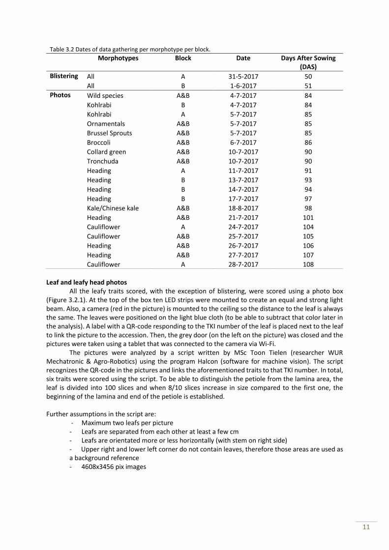
Table 3.2 Dates of data gathering per morphotype per block. Morphotypes Block Date Days After Sowing

(DAS)

Blistering All A 31-5-2017 50 All B 1-6-2017 51

Photos Wild species A&B 4-7-2017 84 Kohlrabi B 4-7-2017 84 Kohlrabi A 5-7-2017 85 Ornamentals A&B 5-7-2017 85 Brussel Sprouts A&B 5-7-2017 85 Broccoli A&B 6-7-2017 86 Collard green A&B 10-7-2017 90 Tronchuda A&B 10-7-2017 90 Heading A 11-7-2017 91 Heading B 13-7-2017 93 Heading B 14-7-2017 94 Heading B 17-7-2017 97 Kale/Chinese kale A&B 18-8-2017 98 Heading A&B 21-7-2017 101 Cauliflower A 24-7-2017 104 Cauliflower A&B 25-7-2017 105 Heading A&B 26-7-2017 106 Heading A&B 27-7-2017 107 Cauliflower A 28-7-2017 108

12

Figure 3.2.1 Picture to illustrate the use of the photo box. At the top of the box ten LEDs and a camera are installed.

At the bottom a leaf with a corresponding label are placed on a light blue cloth.

3.2.2 Genomic data 936 sequence based genotyping (SBG) studies are conducted on the total pool of the

aforementioned accessions. Additionally, 123 whole genome sequences (WGS) representatives of the entire B. oleracea collection are generated. SNPs are called by analysing the GWS data, and these are used for a genomic association mapping study. Sequenced based genotype

Sequence-Based Genotyping (SBG) combines restriction enzyme-mediated complexity reduction with the high-throughput sequencing capacity of Illumina platforms to generate sequences around these restriction sites that are preferably evenly distributed over the entire genome (Keygene, n.d.). For sequencing, a method similar to amplified fragment length polymorphism (AFLP) is used. Firstly, restriction enzymes PstI & MseI (Figure 3.2.2) cut the DNA. Secondly, two structure nucleotides (adapters) are aligned to the sticky ends to reduce amplified genome complements are used. The two adapters bind to the PstI restriction site, and are used to track the different accessions. Thirdly, the restricted DNA is amplified by a poly chain reaction (PCR). Since, Pstl has the two additional bases only ¼ x ¼ = 1/16 of all fragments are amplified. A reference genome of B. oleracea is available, it is possible to align the DNA fragments to this reference genome (“Bolbase - B.oleracea genomics database,” n.d.; Cheng, Wu, et al., 2016; Jingyin Yu et al., 2013). The DNA fragments are aligned to the reference genome based on reads, which are clustered, each alignment with less than three polymorphisms is a cluster. Resulting in pooled libraries, since, sequencing is conducted per plant, and the plants have a barcode in the adapters.

PstI MseI

Figure 3.2.2 Cleavage side for the restriction enzymes PstI and MseI used in the amplified fragment length polymorphism study.

13

Population structure Population stratification (allele frequency differences between cases and controls due to

systematic ancestry differences) can give false associations in GWAS (Price et al., 2006). Involving a population structure will help to overcome population stratification. STRUCTURE software uses a Bayesian approach to cluster accessions (Pritchard, Stephens, & Donnelly, 2000; J. Zhao et al., 2010). The data used for STRUCTURE was converted from a VCF format to PGDSpider 2.1.0.3 format. PGDSpider was run with SNP markers and the numeric format has five values: 1. for Guanine, 2. for Cytosine, 3. for Tyrosine, 4. for Adenine and -9 for a missing value (Groot 2017). In March 2017, STRUCTURE was used to establish the population structure k=8 (K is the optimal number of groups), hereby making use of 459 SNP markers equally distributed over the genome, 913 accessions, using three replications, 100,000 burn-in and 50,000 MCMC calculations. However, these results were not satisfactory and therefor STRUCTURE was run again by MSc student Mazadul Islam. STRUCTURE used k=1 to 12, using 913 accessions, 1,376 SNP markers, using five replications with 100.000 BURN IN AND 100,000 MCMC calculations. Even though 10,000 MCMC are sufficient we calculated 100,000, however 15-20 replications was preferred, time limitations determined five replications (Evanno, Rgnaut, & Goudet, 2005).

The output of STRUCTURE was entered in StructureHarvester software to determine the optimal population structure. StructureHarvester provides four graphs, we only use the first and the fourth graph. The first graph represent the likelihood per K, whereby a plateau could indicate the optimal K. The optimal K is then, the K at plateau minus one. The fourth graph represents Δ K, therefore a peak is considered to be the optimal K (Pritchard et al., 2000).

Genome wide association study Association mapping is conducted to establish associations between genotypic data and

phenotypic data, using the program TASSEL. First, three input files were prepared, the SNP data (described in sequenced based genotype), the population structure (described in population structure), to correct the GWAS, and the phenotypic data for the traits under investigation (described in phenotypical data). Second, the genotypic, population structure and phenotypic data (when no block effect was found) is pooled, using intersect joining. Third, two runs using the program TASSEL 5.2.37 were preformed, one with population structure one without, both using a General Linear Model (GLM) to calculate marker-trait associations. GLM ran with 999 permutation to validate the experiment-wise error rate for individual phenotypes (Anderson & Braak, 2006). GLM provides an output of Logarithm (base 10) Of Odds (LOD) scores to check the probability of a locus associated to a trait variation. With the LOD scores, two Manhattan plot were created using TASSEL, one plot with population structure correction, one without. Validating significant associations were determined using False Discovery Rate (FDR) calculations (described in statistical analysis). To establish interesting markers we determined three criteria:

1. The LOD score for markers should be higher than the threshold FDR value. 2. Markers are only selected when GWAS is corrected for population structure. 3. Markers close to each other, flanking regions, are more interesting than single markers.

Since, the probability of interesting genes in that area is higher when the markers are close.

3.2.3 Statistical analysis The program GenStat 18th was used to statistically analyze the phenotypic data. First, all data was checked for a block effect, running an one-way ANOVA (in randomized block) with the genotype and the block. When this resulted in a P-value > 0.05 a block-effect was not considered. Therefore, the data of the two blocks could be averaged per accession. Secondly, a Quantile-Quantile plot (Q-Q plot) was calculated to check normality assumptions. Results were displayed in boxplots, also made using GenStat.

14

To determine significant differences between the different morphotypes Fisher’s Protected Least Significant Difference (LSD) (<0.05) was calculated. To validate the results of GWAS, the False Discovery Rate (FDR) is calculated using Excel. To calculate the FDR the P-value provided by TASSEL is used. The minimum acceptable FDR is 0.01, and for the calculations, the classical one-stage method is used. The first FDR-adjusted p-value a.k.a. q-value which is significant, is inserted in the following formula to establish the threshold for significant LOD scores in a Manhattan plot.

𝑇ℎ𝑟𝑒𝑠ℎ𝑜𝑙𝑑 = −log (10 ∗ 𝑞 − 𝑣𝑎𝑙𝑢𝑒)

3.2.4 Candidate gene Candidate genes were recognized using associated markers identified on Manhattan plots

using the program TASSEL. A marker is thought to be significantly associated to a trait when the LOD-score is higher than the threshold (established by calculating the FDR). When a candidate marker is found, its location is determined using TASSEL. Then, the location is converted to a candidate region, making us of the average LD for B. oleracea. As the average LD is 36.8 Kb, the search window for the candidate region was set to 50 Kb on both sides (Cheng, Sun, et al., 2016). The candidate region is entered in the genome browse function in BolBase (a comprehensive genomics database for B. oleracea). So far, Bolbase database consists of 630Mb genome sequences, with scaffold N50 size 1.457Mb and contig N50 size 26.828Kb (“Bolbase - B.oleracea genomics database,” n.d.). All genes found in the candidate region were saved and checked for their function either in TrEMBL (TrEMBL is a computer-annotated protein sequence database supplementing the Swiss-Prot Protein Sequence Data Bank) or in Swiss-Prot (comprehensive, high-quality and freely accessible resource of protein sequence and functional information). Additionally, the candidate genes are compared to literature studies such as Cheng, Sun et al., 2016 and Kalve et al., 2014 and previous research by MSc students Floris Slob, Fabian Topper and Twan Groot. When a candidate gene was mentioned in any of these sources the gene was considered for further analysis.

3.2.5 Validating candidate genes To validate the candidate genes found using GWAS a PCR study is conducted. Primers are used

to amplify defined regions of the genome and therefore primers can be used to detect the presence of allelic variation in the genes underlying these traits (Collard & Mackill, 2008). First, these allelic differences for the candidate genes are found by checking the 123 dataset of WGS, with respect to phenotypic variation and morphotypes. Then these genes, and specifically the regions where the SNPs are, are selected on the their uniqueness regarding paralogous. Since, the genus Brassica have undergone a WGT, many paralogous can be found over the entire genome. To search for these paralogous, BRAD (Brassica database) is used to blast the gene sequence to find paralogous. When an unique gene was found, the gene sequence, of these genes is checked for restriction sites using the software program ApE. When a SNP is found in the restriction site of a restriction enzyme the gene is useful, since, it can be used to make a Cleaved Amplified Polymorphic Sequences (CAPS) marker. A CAPS marker is recognizable because the PCR product is either cut or not cut, therefore it is easy to detect if the gene has the SNP of or not. All combinations with genes and restrictions enzymes are first tested on a sub-set of the data containing a variety of different morphotypes (red cabbage, white cabbage, savory cabbage, pointed cabbage, kale, Brussel sprouts, kohlrabi, wild type, collard green, tronchuda, broccoli and cauliflower), before the treatment is applied on 400 accessions (Appendix IV).

The protocol of the PCR method used is found in Appendix V.

15

4 Results

In this chapter, the results obtained in this research will be presented, starting with the phenotypic results in section 4.1. Section 4.2 presents the genotypic results such as, population structure and GWAS. Followed by candidate markers found in candidate regions for leaf blistering and cabbage head weight will be presented in section 4.3. Lastly, specific candidate genes for the aforementioned traits are presented in section 4.4.

4.1 Phenotypic results In this section, the phenotypical results obtained in this study are shown. Starting with the

picture analysis of the photo traits in sub-section 4.1.1. Followed by the results of non-photo traits in sub-section 4.1.2.

4.1.1 Photo traits Photo traits are scored by photographing from six plants (three per block) largest detached

leaf for each accession in the experiment/field. Then, the pictures are analyzed using the software

Halcon. Halcon uses a script to analyze the pictures to retrieve the six leafy traits (lamina length, lamina

width, lamina area, petiole length, petiole width and petiole area). Figure 4.1.1 shows two kale leaves

analyzed by Halcon, whereby the green-rimmed area shows the lamina area and the blue-rimmed area

the petiole area. Figure 4.1.1A shows an accurate representation of the true lamina/petiole area

whereas Figure 4.1.1B shows an overestimation of both the lamina and the petiole area. Therefore,

the results obtained by Halcon are not always in line with reality.

Figure 4.1.1 Example of output of Halcon using a kale leaf. The green-rimmed area is considered as lamina area,

whereas the blue-rimmed area is considered as the petiole area. A) Halcon estimated the petiole and lamina area correctly. B) The petiole and lamina area are overestimated.

It was strived to have six replicates of every accession, as per accession and per block three

leaves are taken. Firstly, we checked if there was a block effect between the two different blocks

(Appendix VI). As there was no block effect found in any trait, all data could be averaged. Secondly, the

data is checked for the normality assumption, by a quantile-quantile plot (Q-Q plot) (Appendix VII).

16

Lamina length, petiole length, and lamina area are considered to be normally distributed. Even though

lamina width at the upper right corner seems not to be normally distributed, we consider it to be

because of the limited dimensions of the photo box. When the leaf was larger than the box the leaf

was broken at the petiole, the size was therefore not correctly measured. Petiole area and petiole

width are not normally distributed. However, as can be seen in Figure 4.1.1A the petiole and lamina

area are related since the green rimmed area and blue rimmed area are touching, therefore the entire

dataset is unreliable.

4.1.2 Non-photo traits In total two non-photo traits were scored: leaf blistering and cabbage head weight. Also for

these traits, block effect and the normality assumption was checked (Appendix VI & VII). Both traits

were not affected by the blocks and the normality assumption was uphold. In Figure 4.1.2A the

variation of leaf blistering between and within the different morphotypes is shown. The highest

variation in leaf blistering is found in heading cabbages and kale, whereas Chinese kale shows the

lowest variation. Figure 4.1.2B represents the level of leaf blistering for the sub-morphotypes of

heading cabbages. Red cabbage has the lowest level of leaf blistering, whereas savoy cabbage has the

significantly highest level of leaf blistering. In Figure 4.1.2C the variation of head weight between the

sub-morphotypes is shown, savoy cabbages are significantly lighter than the other morphotypes.

17

Figure 4.1.2 Box plots representing the variation in non-photo traits among the different Brassica oleracea morphotypes. Letters on the x-axis indicate the significant differences calculated by Fishers protected LSD (<0.05). A)

Level of leaf blistering per morphotype. B) Level of leaf blistering per cabbage sub-morphotype. C) Cabbage head weight per sub-morphotype.

4.2 Genotypic results In this section the genotypic results obtained in this study are shown. Starting with the

population structure in sub-section 4.2.1, followed by the GWAS in sub-section 4.2.2.

4.2.1 Population structure The population structure is determined by running STRUCTURE and StructureHarvester

software. To establish the optimal K a plateau should be recognized in the graph: mean LnP(K) and K (Figure 4.2.1A). When a plateau is found the optimal K is K-1. In the graph: ∆K and K (Figure 4.2.1B) a peak represents an optimal K (Pritchard et al., 2000). So, in order to find the optimal K a plateau should be recognized in Figure 4.2.1A and a peak should be recognized for the same k-value in Figure 4.2.1B (Evanno et al., 2005). However, in Figure 4.2.1A a plateau is not clearly visible, one could argue a plateau can be seen at K=4, K=6 and K=8. Therefore, the optimal K could be K=3, K=5 and K=7. With this information in Figure 4.2.1B a peak can be identified at K=2 and K=5. We selected K= 5 as optimal population structure.

Figure 4.2.1 Output of StructureHarvester for establishing the population structure using the mean LnP(K) with error bars (A) and delta K (B).

18

After establishing the optimal population structure as five, a bar plot is given to show the

distribution of the accessions over the whole collection (Figure 4.2.2). Every vertical line in the bar plot

represents one accession, the distribution of colors of the accessions represent the K-groups where

the accessions belong to. Therefore, the majority of the accessions are considered admixture.

Figure 4.2.2 and Table 4.2.1 show that K1 represents a rest group consisting of collard green,

kale, kohlrabi, tronchuda and wild oleracea; K2 consists merely of heading cabbages, and ornamentals;

K3 almost solely consists of cauliflower; K4 consists merely of sprouts and C9 species; K5 almost solely

consists of broccoli accessions.

Figure 4.2.2 Bar plot output of StructureHarvester, division of morphotypes per k-group.

Table 4.2.1 shows the distribution of the morphotypes per k-group. The total number of 872

accessions, which includes the K<0.50 admixture accessions, is lower than the 913 accessions grown

on the field. This lack of 41 accessions is either due to the fact that the plants did not grow, and

therefore the morphotypes were not verified, or the morphotype was undefined when the plants had

reached maturity. Some accessions were non-replicable, meaning that in at least one of the five

replications the accession is not grouped in the same k-group. In choosing the optimal k-group, group

six and eight are, therefore, deselected as candidate population structure since the number of non-

replicable accessions was significantly higher (337 and 797 respectively). The two non-replicable

accessions were deleted from the dataset, as we used the k-groups as reference in further studies.

K1 group is considered the rest group, so various different morphotypes are present in this

group. Kohlrabi has the highest K-values so fits best, then a mixture of tronchuda, Chinese kale, collard

greens, kale and heading cabbages follows. The heading cabbages found in K1 are generally genebank

accessions from the Mediterranean region. So, K1 represents the rest group where the morphotypes

are more basic and/or less developed, compared to for example cauliflower and cabbages. K2 consists

merely of heading cabbages and ornamentals. Red cabbages have the highest k-value (meaning the

percentage of alleles fitting in K2 is highest), followed by a mixture of white, pointed, and savoy

cabbages. Ornamentals have a low k-value in K2, although they still fully fit into K2. K3 almost solely

consist of cauliflowers. The C9 species have the highest k-value in K4 followed by the sprouts. K5 almost

solely consists of broccoli accessions.

When considering the morphotypes individually, the wild types and the C9 species are the

most diverse morphotypes representing in the different k-groups. Collard green has relatively the most

accessions which do not fully belong to one group. These three morphotypes are therefore, considered

to be the most admixed.

19

Table 4.2.1 Output of StructureHarvester, the different morphotypes are divided in the five groups. Four

accessions are not replicable, they were in different classes during the five replications and therefore not taken into account. Additionally, the accessions which had a k-value <0.5 are not taken into account.

Morphotypes K1 K2 K3 K4 K5 Sum Total K-value <0.50

Not replicable

C9 species 7 1 2 20 0 30 38 8 0

Broccoli 9 1 0 0 57 67 85 18 2

Cauliflower 7 2 193 0 3 205 218 13 0

Collard Green 6 1 0 0 0 7 22 15 1

Heading 45 229 0 1 1 276 294 18 0

Kale 26 1 0 3 0 30 43 13 0

Ornamental 0 17 0 0 0 17 26 9 0

Kohlrabi 45 1 1 0 0 47 48 1 1

Sprouts 1 2 0 44 0 47 49 2 0

Tronchuda 24 0 0 0 0 24 25 1 0

Wild oleracea 5 3 0 0 0 8 16 8 0

Off types 2 2 1 0 2 7 8 1 0

Total 177 260 197 68 63 765 872 107 4

4.2.2 Genome wide association study

Figure 4.2.3 Manhattan plot as a result of the GWAS run by TASSEL, the arrows indicate the candidate markers. A) Head weight with population

sturcture the FDR threshold is 4.97. B) Head weight without population sturcture the FDR threshold is 4.25. C) Leaf blistering with population sturcture the FDR threshold is 3.35. D) Leaf blistering without population sturcture the FDR threshold is 2.68.

20

GWAS is conducted for the traits leaf blistering and cabbage head weight. Every marker (in

total 18,580) is tested if it is significantly associated with a trait. The Manhattan plot shows all the

markers as a dot (Figure 4.2.3). When a dot is above the threshold, it is thought to be significantly

associated to the trait. To establish significantly associated markers the FDR (>0.01) is calculated, the

threshold is seen in Figure 4.2.3 as the black solid line in the Manhattan plots.

In Figure 4.2.3A and Figure 4.2.3B the arrows represent the identified candidate markers. To

identify candidate markers from the Manhattan plots five criteria are used.

1. The LOD score for markers should be higher than the FDR value. 2. Markers are only selected when GWAS is corrected for population structure. 3. Markers close to each other, flanking regions are more interesting than single markers. 4. Allelic composition in relation to trait. 5. Identify same marker region in independent experiments (2015, 2016).

For both traits, a comparison between association mapping with or without population

structure correction is made. Table 4.2.2 shows the number of significant markers per trait. When

comparing the number of significantly associated markers, the number in without population structure

correction is considerably higher. It is thought to reduce the number of false positives when the

population structure is taken into account. However, the number of significantly associated markers

using population structure correction for leaf blistering is still high, which might suggested that the

threshold calculated by FDR, is too low.

4.3 Candidate markers Based on the three aforementioned criteria, in total, seven interesting markers are found for

leaf blistering, and fifteen for head weight (Figure 4.2.3). To continue the quest to find candidate genes

for leaf blistering and head weight, these candidate markers are transformed into candidate regions.

The candidate markers are translated to candidate regions, by adding 50kb to both sides of the marker

(Table 4.3). As the average LD is 36.8kb the search window is slightly higher to account for any unevenly

distributed markers (Appendix III).

Additionally, the candidate markers are compared based on their LOD score. The overall TKI

research project has been running for several years now. Therefore, there are datasets available from

2015 (Floris), 2016 (Companies & ZonMW) and the data collected in 2017 (this thesis). In the previous

studies, not all accessions were grown and different traits were scored, additionally, different methods

are used for scoring the traits. However, as the raw data of all experiments is still available, TASSEL is

ran again, making use of the population structure correction K=5 (Table 4.3). For the datasets Floris

and ZonMW the FDR threshold value is calculated and the significantly associated markers are

highlighted in yellow.

Table 4.2.2 Number of associated markers found in GWAS with population structure correction and without. Traits # Markers

With population structure correction

# Markers Without population structure correction

Leaf blistering 822 3865

Head weight 19 100

Total 841 3965

21

Table 4.3 Overview of the candidate markers, their location, allele frequency and their corresponding -10log (LOD) scores in the different datasets. The LOD scores highlighted in yellow show a significantly associated marker to the trait.

Trait Peak marker Candidate region (bp)

Allele frequency

LOD score

LOD Companies

LOD Floris

LOD ZonMW

C03 16946055 16896055..16996055 89%C 11%G 13.36 0.71 NA NA C04 20520782 20470872..20570872 75%C 25%G 12.78 1.1 NA NA Leaf C04 34477381 34427381..34527381 88%G 12%T 13.76 1.4 NA NA blistering C05 10319967 10269967..10369967 87%T 13%C 9.22 1.4 NA NA C06 18873634 18823634...18923634 97%T 3%G 8.70 0.16 NA NA C07 5829451 5779451..5879451 95%G 5%A 10.76 2.7 NA NA C08 14790421 14740421..14840421 97%C 3%T 8.52 2.67 NA NA

C01_33540674 33490674..33590674 55%G 45%C 5.45 0.2 4.1 1.9 C01_33540749 33490749..33590749 53%G 47T% 5.03 0.03 3.8 1.6 C03_6843849 6793849..6893849 52%T 48%C 5.23 1 1.4 0.297 C03_6843822 6793822..6893822 52%A 48%G 5.08 - 2 0.155 C05_26114270 26064270..26164270 96%T 4%C 5.11 1.6 1.4 0.9 C06_3121203 3071203..3171203 70%G 30%T 5.20 1.8 1.2 1.1 Head C06_20826427 20776427..20876427 97%A 3%G 5.55 1.6 4.8 0.8 weight C07_35662758 35612758..35712758 87%A 13%T 5.35 0.02 0.4 3.6 C08_35892752 35842752..35942752 69%T 31%C 5.12 0.006 3.4 1.4 C08_31561734 31511734..31611734 80%T 20%C 5.14 1.1 2.1 2.2 C09_12411624 12361624..12461624 73%C 27%T 5.23 0.2 4.9 3.6 C09_27943876 27893876..27993876 69%C 31%T 5.83 - 3.4 0.5 C09_27943899 27893899..27993899 70%T 30%C 5.39 0.04 2 0.03 C09_27943857 27893857..27993857 55%C 45%T 5.24 - 3.3 0.1 C09_36633552 36583552..36683552 90%C 10%T 5.60 0.4 0.4 0.2

Furthermore, the allele frequency of the peak markers is checked, for further analysis it seems

favorable to have a somehow equally distributed allele frequency. The data is initially checked for a

minor allele frequency (MAF) of >2.5. However, when the dataset is small, as in cabbage head weight,

the number of accessions carrying a specific allele can become too small to statically analysis (Figure

4.4.1 and Appendix VIII).

4.4 Candidate genes The candidate regions are entered into BolBase to check which genes are present. For leaf

blistering, in total 45 candidate genes are found, for head weight 47 (Appendix IX). The candidate genes

found in the candidate regions are validated on multiple areas. Firstly, the function of the gene is

checked using Swiss-Prot and TrEMBL. Secondly, the candidate genes are compared to current

literature studies in Brassica as well as Arabidopsis, such as Cheng, Sun et al., 2016 and Kalve et al.,

2016. Thirdly, the genes are compared to the candidate found by MSc students Floris Slob, Fabian

Topper and Twan Groot. This resulted in four candidate genes for leaf blistering, and eight candidate

genes for head weight (Table 4.4).

22

Table 4.4 Overview of candidate genes, their location and function (“UniProt,” n.d.).

Gene Location Function

Head weight

IAA19 C01: 33575783 : 33576943 Auxin response gene PME35 C08: 31567374 : 31567961 Acts on primary cell wall pectin in the stem PAR2 C08: 31548318 : 31548644 Negative regulator of shade avoidance syndrome PAP1 C09: 12427433 : 12433563 Involved in light/cold stress related jasmonate biosynthesis APUM19 C09: 27967024 : 27967566 Involved in the regulation of vegetative development TOE2 C09: 27946639 : 27949476 Negatively regulates the transition to flowering APRR3 C09: 27914944 : 27917092 Controls photoperiodic flowering response, circadian clock ZFP3 C09: 36642009 : 36642737 Involved in ABA hormone regulation

Leaf blistering

TCP4 C03: 16936104 : 16937318 Transcription factors essential in leaf growth SPL3 C04: 20510435 : 20510961 Promotes the vegetative phase change ARF3 C04: 20533558 : 20536202 Leaf polarity development OFP16 C04: 34484983 : 34485693 Regulates plant growth and development

Figure 4.4.1 shows box plots displaying the variation of alleles for the two markers C03

16946055 and C04 20520782 which are involved in leaf blistering as it was found in the dataset of

2017. Additional boxplots for all the candidate markers detailed in Table 4.4 are shown in Appendix IX.

Figure 4.4.1 Variation of leaf blistering for different allelic composition in each k-group for the candidate marker C03 16946055 (A) and C04 20520782 (B) in the dataset of 2017. The quadrant represents the variation of

leaf blistering for the allelic composition, the number represents the amount of plants showing this allele. The letters show significant differences between the levels of leaf blistering and the allelic composition per k-group.

Interestingly, leaf blistering in K2 is significantly different for the allelic composition in all

candidate markers. The level of leaf blistering appears to be higher when plants are homozygous for

GG compared to CC. However, it might be to progressive to draw conclusions from the boxplots shown

in Figure 4.4.2 and Appendix IX since the number of replicates for specific allelic compositions is low.

K2 consist of all ornamentals and the majority of the heading cabbages.

23

Figure 4.4.2 Variation of cabbage head weight for different allelic composition in each sub-morphotype for the candidate marker C01 33540674 (A) and C01 33540749 (B) in the dataset of 2017. The quadrant represents the variation of head weight for the allelic composition, the number represents the amount of plants showing this allele. The letters show significant differences between the head weight and the allelic composition per sub-morphotype.

Similar to the allelic composition of leaf blistering the two most striking candidate markers for

cabbage head weight found in the dataset of 2017, are displayed in Figure 4.4.2. The markers C01

33540674 & C01 33540749 are relatively close to each other, therefore, the trend in the figures are

alike. Accessions with different alleles for both markers are significantly different in head weight in

savoy cabbages, where the homozygous CC allele has a significantly higher cabbage head weight than

the homozygous GG of heterozygous state in marker C01 33540674. The same holds for marker C01

33540749 where the homozygous TT allele are responsible for a higher head weight than the

homozygous GG of heterozygous state.

First, the candidate genes are checked for the presence of any paralogous, because if there are

any paralogous in the genome, the result can be a false positive. When no paralogous genes could be

found, ApE is used to check if the candidate genes have a unique cutting site, for the restriction

enzyme. Additionally, there is checked if the restriction enzyme has another cutting site in the

candidate gene, as this could also give a false positive error. Finally, OFP16 has two unique SNPs in the

candidate gene region where restriction enzymes Acclll and BsiWl could cut. Additionally, ZFP3 has one

unique cutting site for the restriction enzyme Psil. After selecting these three candidate genes +

restriction enzyme combinations, these are checked on a subset of the morphotypes. The subset was

used to verify the primers and restriction enzymes, as they hypothetically should work on at least some

of the 96 accessions. Additionally, the subset of morphotypes was used to create a good overview of

the genes and their poly-allelic differences over the collection, as the variation in the collection is high.

Unfortunately, the results of the ZFP3+PsiI experiments were not as hoped for, the ZFP3 gene

did not show any products/bands in the PCR study and therefore these are not used in this study

(Figure 4.4.3A). OFP16 is a gene with 710 base pairs, having eleven known polymorphisms in our

dataset, two of those polymorphisms are in a restriction enzyme cutting site position: 275 for AccIII

and 424 for BsiWI. OFP16 cut by restriction enzyme AccIII did not gave any results with separate bands

(Figure 4.4.3B). This could mean the restriction enzyme was not able to cut, or although less likely, the

accessions were all homozygous for this polymorphism in the OFP16 gene. When the PCR product of

OFP16 was cut with the restriction enzyme BsiWI, different bands were detected. One band on the top

means the restriction enzyme was not able to cut, so the accession did not have a polymorphism. Two

24

bands means the accession is homozygous for the polymorphism. Three bands means the accession is

heterozygous for the polymorphism.

PCR ZFP3 PCR OFP16 + restriction enzyme

AccIII

PCR OFP16 + restriction enzyme BsiWI

Figure 4.4.3 Result of validating genes and restriction enzyme combination. A) Result of PCR study conducted on the gene ZFP3, where only a few light bands can be detected. B) Result of PCR study conducted on the gene OFP16 with restriction enzyme AccIII, all bands are semi on the same level. C) Result of PCR study conducted on the gene OFP16 with restriction enzyme BsiWI, 1,2 and 3 separate bands can be detected for the different morphotypes.

In total, the OFP16 + BsiWI combination is tested on a subset of 400 accessions (Figure 4.4.4). The total number of occurrence for a band/band combination in a morphotype is summed. The distribution of bands in white cabbage could be interesting, by far most of the white cabbages had only one band, meaning they are homozygous to not have the polymorphism. On the other hand, about 1/3 of the accessions display three bands meaning that those accessions are heterozygous for the polymorphism. Additionally, cauliflower has an interesting distribution of bands whereby three bands, the heterozygous genotype occur far more often than the other genotypes.

Referring back to the level of leaf blistering per morphotype in Figure 4.1.2A, broccoli, Chinese

kale, collard green and kale show the highest level of leaf blistering. Figure 4.1.2B shows that savoy

25

cabbages has the highest level of leaf blistering, followed by white and pointed cabbages, red cabbages

show almost no leaf blistering. Looking at Figure 4.4.4 savoy cabbages and broccoli have relatively

often three bands, so are often heterozygous to the polymorphism. However, white cabbage, kale,

collard green and Chinese kale counteract this trend, by having only one band and are therefore

homozygous for the polymorphism. One could argue that have at least one polymorphism increases

the leaf of leaf blistering.

Figure 4.4.4 Boxplot of the frequency of the number of bands per morphotype.

26

5 Discussion

In this chapter, the results obtained in this research will be discussed, starting with the phenotypic results in section 5.1. Section 5.2 discusses the genotypic results such as, population structure and GWAS. Lastly, in section 5.3 quest for the candidate genes is discussed.

5.1 Phenotypic In this section, the phenotypical results obtained in this study are discussed. Starting with the

field trial in general as all phenotypic data is gathered on the field in sub-section 5.1.1. Subsequently, the picture analysis of the photo traits in sub-section 5.1.2. Followed by the results of non-photo traits in sub-section 5.1.3.

5.1.1 Field trial

The field trial was designed for 913 accessions, in the end 842 accessions were grown on the field due to poor seed quality and germination problems. Two clusters of data were gathered: leaf traits and cabbage head traits. To obtain a fair and good overview of the traits, data was gathered in a short time, so the plants were in the same developing stage. Scoring traits was done per morphotype and per block, for example kohlrabi block A was scored on 84 DAS and kohlrabi block B was scored on 85 DAS, to minimize growth development. Although for morphotypes consisting of many accessions, such as cabbages, the process might have took too long. The cabbage leaves had grown in the meantime so comparing in between one morphotype was not fair. Additionally, comparing between morphotypes is not fair, since, there was a lot of time between the harvesting periods. The harvesting period in this case took almost one month, the first morphotypes harvested, grew almost certainly bigger in the meantime. Since, this study makes use of population structure where different morphotypes were clustered, this could result in errors in the data. Further studies could account for this by comparing the leaves/plants harvested in the beginning to the same leaves/plants harvested in the end.

Scoring head traits was slightly more difficult as the cabbages needed to be harvested and therefore they should be fully matured. As the collection of heading cabbages was large and summer and winter types were admixed, we manually selected the mature cabbages on the field. To preserve an objective view, harvesting was done with two people. However, especially for the savoy cabbages, it was difficult to judge maturity as the leaves had more severe blistering than the other cabbage varieties. Due to the blistering, the savoy cabbages had a loose structure, which made it difficult to estimate the maturity, since the selection was partly based on estimation the head density. Previous studies (2015&2016) harvested all the cabbage heads at once, so even when cabbages were not fully maturated, as the objective of those studies were leaf and head development. However, during this experiment the decision was made to study the matured heads, in order to develop more knowledge on cabbage heads on itself. Although, leaf development was also in the interest of this research, and therefore the developmental leaves of cabbages were harvested and photographed.

Leaf traits were partially scored taking photos (sub-section 5.1.2) and by scoring the level of leaf blistering by walking through the field and scoring manually (sub-section 5.1.3).

5.1.2 Photo traits The photos of the detached leafs were analysed using the software Halcon. Toon Tielen designed a script to estimate six leafy traits (lamina length, lamina width, lamina area, petiole length, petiole width and petiole area). However, in this research, the variety of accessions and morphotypes was high and the variety of leaves was even higher, some leaves had lobes on the petiole while others did not even have a petiole. Therefore, it was difficult to develop one script, that could incorporate all the variation and would still be accurate. For example, Figure 4.1.1 shows the difficulty in establishing

27

the edge of the leaf, the edge of the leaves of the varieties were so different and are therefore difficult to recognize by Halcon. Additionally, mud on the cloth made it difficult to distinguish the leaf. Furthermore, figure 4.1.1 shows that it was difficult to differentiate the petiole area from the lamina area, since many accessions have lobes on their petiole. To distinguish the petiole from the lamina the leaf is divided into 100 slices and when 8/10 slices increase in size compared to the first one, the beginning of the lamina and end of the petiole is established. Since these areas are linked, when one is wrongly estimated the other one will be as well. To overcome this problem, a ruler could have indicated the border, or the leaf could be cut at the petiole/lamina border so the script would not have to establish that. The similar software program ImageJ verified the data provided by Halcon. ImageJ is less accurate in estimating the leaf edge and in our case, less user friendly. Several pictures of leave were analyzed using both programs, resulting in different estimations of lamina and petiole area. Additionally, Halcon sometimes did not recognize the leaf but mud instead, or recognized two leaves when there was only one. Furthermore, when the data produced by Halcon was checked for normality, it was not uphold. In addition to the wrong estimation of the lamina/petiole distinction, it was decided that the data obtained by photographing and analyzing by Halcon was not accurate enough, and therefore, not taken into account in further analysis. Initially, focus was on leaves as well as cabbage heads, therefore the cabbages were harvested when they had reached maturity. Then the heads were weighted and cut in half to be photographed. Due to time limitation, a script was not developed to analysis these pictures. Moreover, developing leaves in heading cabbage were harvested to compare those to matured leaves. However, due to time limitation a script specifically for these leaves was not developed and the developing leaves were not taken into account in the analysis.

5.1.3 Non-photo traits In total, two non-photo traits were scored: leaf blistering and cabbage head weight. The same

person, to reduce bias, scored leaf blistering of all accessions, in two succeeding days. The scoring was based on the classes of leaf blistering in cabbages defined by the UPOV. In the field an example sheet of the different classes was used to be able to constantly verify the scoring.

Cabbage head weight was scored using a weight scale on the field, so the cabbages were harvested and weighted as soon as possible to reduce evaporation. Red cabbages are significantly the lightest sub-morphotype in this research. White, pointed and savoy cabbages are not significantly different from each other. White cabbage displays the most variation in cabbage head weight whereas pointed cabbages shows the least variation. This could be due to the number of accessions, respectively 204 and 9 accessions. For further studies, it is recommend to have a more equally distributed collection, to validate the results. Additionally, early and late maturing varieties are admixed, making the harvest and the processing of the data difficult. Early maturing varieties start forming a head without expending excess growth in wrapper leaves, making it more difficult to estimate the maturity of the cabbage (Tanaka & Niikura, 2003). Furthermore, savoy cabbage has the highest level of leaf blistering and is also the lightest morphotype. This can either be true, since savoy cabbages are known for their loose structure. Alternatively, the savoy cabbages are harvested too early and the savoy cabbages did not reach maturity yet, and are therefore the lightest.

5.2 Genotypic In this section the genotypic results obtained in this study are discussed. Starting with the

sequence data in sub-section 5.2.1. Population structure is discussed in sub-section 5.2.2, followed

by the GWAS in sub-section 5.2.3.

5.2.1 Sequence data The sequence based genotype data, containing 18,580 markers, was used in this study as input for the GWAS. The karyotype (Appendix III) shows the distribution of the markers over the

28

chromosomes. Generally, the karyotype shows markers distributed all over the genome, however chromosome two and nine are less densely packed with markers. This could implement that some regions in the genome were not mapped completely, leaving some regions/haploblocks unmapped. Therefore, a LD analysis could be useful, to understand the recombination variation in regard of the total genome, to eventually have a full coverage of the genome.

5.2.2 Population structure Population structure was calculated at the start of 2017 by MSc student Twan Groot, however

to verify these outcomes MSc student Mazadul Islam calculated the population structure in this

research again. The outcome, which is therefore more reliable now, was five k-groups instead of eight

calculated by Twan. The number of k-groups was established by considering the graphs provided in

Figure 4.2.1, based on the approaches explained by Pritchard et al. (2000) and Evanno et al. (2005).

The outcome of Prichards method is shown in Figure 4.2.1A, the error bars indicate that the variation

in the data is low, which is preferable. However, in this case, a clear plateau was difficult to define.

Therefore, another graph (Figure 4.2.1B) was taken into account; Evanno et al. (2005) developed a

method based on the outcome of Pritchard’s method to determine the population structure. Although

Evannos method is mathematically questionable since two ratio are divided, it helps establishing the

population structure. This method provides a graph where peaks qualify as optimal k-groups. When

reviewing both graphs the optimal k-group in this thesis is five.

Even though, these graphs were not ultimately convincing, the consistence of the groups is

explainable. Pelc et al. (2015) preformed a PCA study (explained below) in Brassica, in which 30.1% of

the variation was explained the following groups form: 1) Portuguese cabbage, collard green, Brussel

sprout and cabbage 2) cauliflower and broccoli 3) kale (Pelc, Couillard, Stansell, & Farnham, 2015).

Which is in line with the results found in this study, K1 consisting of kohlrabi, tronchuda, Chinese kale,

collard greens, kale and heading cabbages, the more basic morphotypes. Furthermore, the

morphotypes cauliflower and broccoli are more or less distinguishable groups in both studies. This can

also be seen in Figure 1.3.

To verify the optimal k-group five, other methods can be used, such as; unified mixed-model,

and Principal Component Analysis (PCA). The unified mixed model developed by Yu et al. (2006), uses

pairwise kinship coefficients, the relatedness among individuals within and between subpopulations,

to assign individuals to sub-populations (Jianming Yu et al., 2006). The unified mixed-model is thus

suitable for association mapping with multiple levels of relatedness, and would therefore be

interesting in this research. However, in a B. rapa study the kinship method was not proven to be

helpful therefore it might be also not helpful in B. oleracea (J. Zhao et al., 2010). Additionally, PCA

could be interesting in this research; PCA was originally used in humane disease studies, however it

could be implemented in this type of research. PCA can be used to summarize genome-wide patterns

of relatedness (Price et al., 2006). The advantages of PCA, compared to STRUCTURE are that it is less

computationally intensive and easier to use in big datasets.

5.2.3 Genome wide association mapping The five criteria, high LOD (-log10) score, >FDR threshold, interesting flanking regions, function

and previous studies resulted in fourteen candidate markers. The advantages and disadvantages of the

criteria are discussed later. For blistering the following markers are found: C03 16946055, C04

20520782, C04 34477381, C05 10319967, C06 18873634, C07 5829451 and C08 14790421 and

C01_33540674, C01_33540749, C08_31561734, C09_12411624, C09_27943876, C09_27943899,

C09_27943857 and C09_36633552 for head weight. In this GWAS study, after comparing, the

population structure correction was always taken into account (Figure 4.2.3). However, when

accounting for the population structure, false positives should not be incorporated. In this case, the k-

29

group specific markers. Furthermore when population structure correction is used, the risk of

introducing false negatives increases (K. Zhao et al., 2007).

For head weight only 19 markers were found, whereas 822 markers were associated to leaf blistering. The number of markers associated with leaf blistering therefore seemed abnormally high. This could be due to the FDR (<0.01) which was not strict enough, or accessions showing leaf blistering have a similar extensive growing pattern causing many genes to be involved in the process. When the FDR threshold is not sufficient, unified mixed-model or PCA could be used to have a securer regime.

The criteria of a high LOD score has a disadvantage that the score is not influenced by the population structure correction and therefore the trait could be sub k-group specific and not trait specific. To overcome this disadvantage, the LOD score without population structure can be taken into account for example when the LOD score after population structure correction is higher than the LOD score without population structure correction the candidate marker is likely to be a true positive.

Additionally, the data scored previously in the TKI project was used to verify the candidate regions. The raw phenotypic data of three datasets, and the new population structure correction was entered in TASSEL to perform a GWAS. The population structure correction could be used since the same accessions were used. However, the phenotypic data was collected using a different method, the leaf blistering scored in 2015 was for example scored on a 0-9 scale where in this study a 0-7 scale was used. In addition, the cabbage head weight was measured differently since, previous harvests all cabbages were harvested at once, so some accessions might have not reached maturity. The results of the GWAS with old data confirmed some markers in head weight (9/15). This means that also in the old data that candidate marker was significantly associated with the trait. Additionally, the regions of interest, so the candidate marker and the flanking regions, were often comparable. However, in leaf blistering none of the candidate markers was validate, this might have to do with only one data set available and the different research method. Therefore, the data scored in 2015 and 2016 was not leading and only used as a reference.

Finally, the whole genome sequence (WGS) data was used in this study as a validation for choosing candidate markers. The dataset consisted of in total eight morphotypes, and their allelic polymorphism information. Since the WGS data was not linked to the TKI data, the data had to generalized to morphotypes, and TKI-accessions could not specifically pinpointed.

5.3 Candidate gene The candidate markers identified by the GWAS study were converted into a candidate region in which candidate genes were selected. The average LD of brassica crops is 36.8 kb (Cheng, Sun, et al., 2016). However, as can be seen in Appendix III the marker density is not equally distributed over the genome, therefore a flanking region of 50 kb was used. In total, 45 candidate genes for leaf blistering and 47 candidate genes for cabbage head weight were found in the candidate regions. An important aspect to take into account is that many of the genes mentioned below and their function is known because of studies in Arabidopsis and their function in brassica is still largely unknown. However, the hypothesis is that genes found in Arabidopsis have a similar function as the same genes in Brassica since the nucleotide sequence is 75-90% similar in exons (Ayele et al., 2005). The four candidate genes for blistering are: TCP4, SPL3, ARF3 and OFP16.

The function of TCP genes, is described by Kalve et al. 2014 as cell division promoting, and therefore an essential regulator in leaf growth. In Arabidopsis thaliana up-regulation of miR319 inhibits the expression of TCP4 and other TCP-genes, resulting in bigger and wrinkled leaves (Palatnik et al., 2003). Additionally, of TCP4 is associated with a round head shape in brassica rapa (Mao et al., 2014).

SPL3 is part of the SQUAMOSA PROMOTER BINDING PROTEIN-LIKE family (SPL3). Overexpressing of SPL3 abaxial trichome production and short petioles and regulates phase-specific patterns of leaf epidermal differentiation and flowering time (M. Walker, Kublin, & Zunt, 2009). An

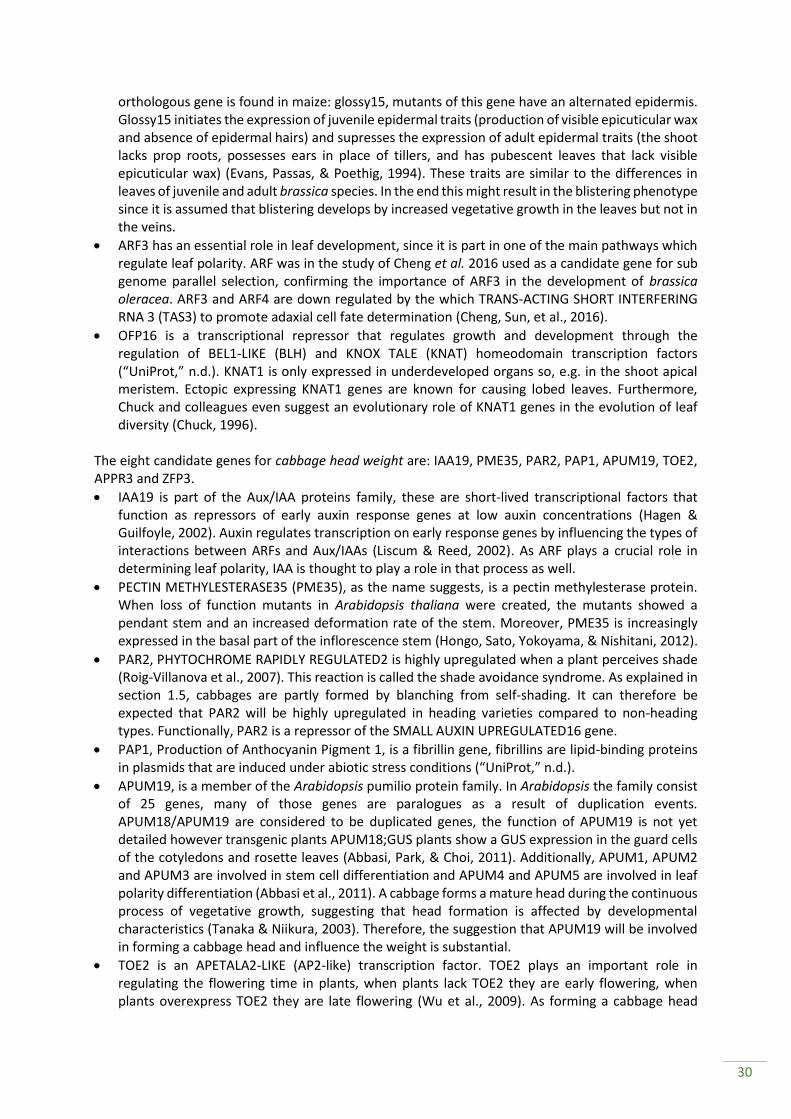
30

orthologous gene is found in maize: glossy15, mutants of this gene have an alternated epidermis. Glossy15 initiates the expression of juvenile epidermal traits (production of visible epicuticular wax and absence of epidermal hairs) and supresses the expression of adult epidermal traits (the shoot lacks prop roots, possesses ears in place of tillers, and has pubescent leaves that lack visible epicuticular wax) (Evans, Passas, & Poethig, 1994). These traits are similar to the differences in leaves of juvenile and adult brassica species. In the end this might result in the blistering phenotype since it is assumed that blistering develops by increased vegetative growth in the leaves but not in the veins.

ARF3 has an essential role in leaf development, since it is part in one of the main pathways which regulate leaf polarity. ARF was in the study of Cheng et al. 2016 used as a candidate gene for sub genome parallel selection, confirming the importance of ARF3 in the development of brassica oleracea. ARF3 and ARF4 are down regulated by the which TRANS-ACTING SHORT INTERFERING RNA 3 (TAS3) to promote adaxial cell fate determination (Cheng, Sun, et al., 2016).

OFP16 is a transcriptional repressor that regulates growth and development through the regulation of BEL1-LIKE (BLH) and KNOX TALE (KNAT) homeodomain transcription factors (“UniProt,” n.d.). KNAT1 is only expressed in underdeveloped organs so, e.g. in the shoot apical meristem. Ectopic expressing KNAT1 genes are known for causing lobed leaves. Furthermore, Chuck and colleagues even suggest an evolutionary role of KNAT1 genes in the evolution of leaf diversity (Chuck, 1996).

The eight candidate genes for cabbage head weight are: IAA19, PME35, PAR2, PAP1, APUM19, TOE2, APPR3 and ZFP3.

IAA19 is part of the Aux/IAA proteins family, these are short-lived transcriptional factors that function as repressors of early auxin response genes at low auxin concentrations (Hagen & Guilfoyle, 2002). Auxin regulates transcription on early response genes by influencing the types of interactions between ARFs and Aux/IAAs (Liscum & Reed, 2002). As ARF plays a crucial role in determining leaf polarity, IAA is thought to play a role in that process as well.

PECTIN METHYLESTERASE35 (PME35), as the name suggests, is a pectin methylesterase protein. When loss of function mutants in Arabidopsis thaliana were created, the mutants showed a pendant stem and an increased deformation rate of the stem. Moreover, PME35 is increasingly expressed in the basal part of the inflorescence stem (Hongo, Sato, Yokoyama, & Nishitani, 2012).

PAR2, PHYTOCHROME RAPIDLY REGULATED2 is highly upregulated when a plant perceives shade (Roig-Villanova et al., 2007). This reaction is called the shade avoidance syndrome. As explained in section 1.5, cabbages are partly formed by blanching from self-shading. It can therefore be expected that PAR2 will be highly upregulated in heading varieties compared to non-heading types. Functionally, PAR2 is a repressor of the SMALL AUXIN UPREGULATED16 gene.

PAP1, Production of Anthocyanin Pigment 1, is a fibrillin gene, fibrillins are lipid-binding proteins in plasmids that are induced under abiotic stress conditions (“UniProt,” n.d.).

APUM19, is a member of the Arabidopsis pumilio protein family. In Arabidopsis the family consist of 25 genes, many of those genes are paralogues as a result of duplication events. APUM18/APUM19 are considered to be duplicated genes, the function of APUM19 is not yet detailed however transgenic plants APUM18;GUS plants show a GUS expression in the guard cells of the cotyledons and rosette leaves (Abbasi, Park, & Choi, 2011). Additionally, APUM1, APUM2 and APUM3 are involved in stem cell differentiation and APUM4 and APUM5 are involved in leaf polarity differentiation (Abbasi et al., 2011). A cabbage forms a mature head during the continuous process of vegetative growth, suggesting that head formation is affected by developmental characteristics (Tanaka & Niikura, 2003). Therefore, the suggestion that APUM19 will be involved in forming a cabbage head and influence the weight is substantial.

TOE2 is an APETALA2-LIKE (AP2-like) transcription factor. TOE2 plays an important role in regulating the flowering time in plants, when plants lack TOE2 they are early flowering, when plants overexpress TOE2 they are late flowering (Wu et al., 2009). As forming a cabbage head

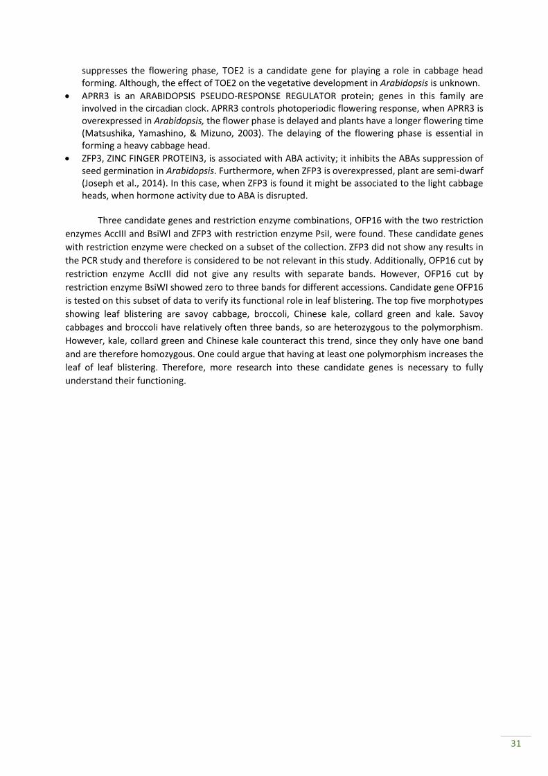
31

suppresses the flowering phase, TOE2 is a candidate gene for playing a role in cabbage head forming. Although, the effect of TOE2 on the vegetative development in Arabidopsis is unknown.

APRR3 is an ARABIDOPSIS PSEUDO-RESPONSE REGULATOR protein; genes in this family are involved in the circadian clock. APRR3 controls photoperiodic flowering response, when APRR3 is overexpressed in Arabidopsis, the flower phase is delayed and plants have a longer flowering time (Matsushika, Yamashino, & Mizuno, 2003). The delaying of the flowering phase is essential in forming a heavy cabbage head.

ZFP3, ZINC FINGER PROTEIN3, is associated with ABA activity; it inhibits the ABAs suppression of seed germination in Arabidopsis. Furthermore, when ZFP3 is overexpressed, plant are semi-dwarf (Joseph et al., 2014). In this case, when ZFP3 is found it might be associated to the light cabbage heads, when hormone activity due to ABA is disrupted.

Three candidate genes and restriction enzyme combinations, OFP16 with the two restriction

enzymes AccIII and BsiWl and ZFP3 with restriction enzyme PsiI, were found. These candidate genes

with restriction enzyme were checked on a subset of the collection. ZFP3 did not show any results in

the PCR study and therefore is considered to be not relevant in this study. Additionally, OFP16 cut by

restriction enzyme AccIII did not give any results with separate bands. However, OFP16 cut by

restriction enzyme BsiWI showed zero to three bands for different accessions. Candidate gene OFP16

is tested on this subset of data to verify its functional role in leaf blistering. The top five morphotypes

showing leaf blistering are savoy cabbage, broccoli, Chinese kale, collard green and kale. Savoy

cabbages and broccoli have relatively often three bands, so are heterozygous to the polymorphism.

However, kale, collard green and Chinese kale counteract this trend, since they only have one band

and are therefore homozygous. One could argue that having at least one polymorphism increases the

leaf of leaf blistering. Therefore, more research into these candidate genes is necessary to fully

understand their functioning.

32

Conclusion & recommendation

Brassica oleracea is, with all the diverse morphotypes, an economical important and health promoting plant family, of which currently insufficient scientific information regarding the genetic variation available is. Therefore, the initial aim of the research was to obtain insight in the genetic variation of the B. oleracea species regarding leaf, head morphology, and development, in a highly diverse collection by conducting an association mapping study. However, due to time limitations and inadequate research methods, results were not sufficient and not validated. Therefore, we were not able to draw the conclusions we hoped to draw. Hence, this thesis project was set as a case study, describing two verified leading examples. Thus, the aim of the thesis was defined as explaining phenotypical variation in leaf development by assessing genetic variation in Brassica oleracea.

Phenotypic variation was scored in two clusters of data: leaf traits and cabbage head traits. Both clusters involved taking photos of the traits of interest and gathering the data manually in the field. To obtain a fair and good overview of the traits there was strived to gather the data in a short time, so the plants are in the same developing stage. However, this was not always possible due to low man power, weather conditions, among others. Future studies could anticipate on this by having a better planning before the start of the experiment. Additionally, having a side experiment where the leaf development and head formation is tracked from day to day by taking pictures, on the field, of a small sub-set of the accessions.

The photos of the detached leafs were analyzed using the software Halcon, however, developing a script to analyze pictures was difficult when the variety in leaf morphology is tremendously high. It is therefore, recommended to develop multiple scripts with morphotype specific requirements. Additionally, in advance incorporating requirements of data input is recommend, for example to define the petiole from the lamina, a ruler could have indicated the line so the script would not have to establish that.

Genotypic variation was gathered on two levels, a whole genome sequence study was conducted on 123 accessions, this dataset consisted of in total eight morphotypes, and their allelic polymorphism information. Secondly, there was the sequence based genotype data, which consist of 18,580 markers distributed over the genome. The karyotype shows that chromosome two and nine are less densely packed with markers. Therefore, a LD analysis would be useful, to understand the recombination variation in regard of the total genome. Additionally, a suggestion would be to perform a whole genome sequence on TKI accessions to be able to check the effect of phenotypic traits, on genome level.

Population structure was calculated to establish a method to correct the GWAS, in this study the population structure was optimal when the number of k-groups is five. The graphs established the optimal k-group were not ultimately convincing looking at Prichard’s graph and understanding Evanos statistical methods, however the consistence of the groups was understandable. To verify the outcome k5, the unified mixed-model and the principal component analysis can be used.

A GWAS study was conducted to find markers, which are associated with either leaf blistering or cabbage head weight, in which, the population structure correction was taken into account. The number of significant marker found for head weight was only 19 markers, whereas 822 markers were associated to leaf blistering (Figure 4.2.3). The number of markers associated to leaf blistering therefore seemed abnormally high. When the FDR threshold is not sufficient unified mixed-model or PCA can be used to have a confident method. Furthermore, a GWAS study only consisting of cabbages could be used, to map more accurately.

The candidate markers identified by the GWAS study were converted into a candidate region in which candidate genes were selected. In total, 45 candidate genes for leaf blistering and 47 candidate genes for cabbage head weight were found in the candidate regions. The candidate genes were then, subjected to a function analysis, in total, four candidate genes for blistering were found: TCP4, SPL3, ARF3 and OFP16. Additionally, eight candidate genes for cabbage head weight were found: IAA19, PME35, PAR2, PAP1, APUM19, TOE2, APPR3 and ZFP3. Eventually, one of the candidate genes proved to play a role in leaf blistering. OFP16 with a polymorphism (A-T) at the 424th position in the

33

gene could play a role in a higher level of leaf blistering. Since, having at least one polymorphism increases the leaf of leaf blistering in some morphotypes. With the data of the frequency of occurrence of the number of bands per morphotype a new GWAS study could be run to validate the candidate gene. In further research, the genes can be verified by looking at the candidate genes more carefully and designing a new candidate gene approach experiment.

To conclude, the field trial was ambitious as the number of accessions was large. However, by taking six pictures of each accession the impact of the data gathered is tremendous and useful for numerous purposes and can be analyzed at any moment. Furthermore, as Brassica is still a crop which is not extensively investigate, the quest for candidate genes is difficult, partly because of the whole genome triplication and the lack of scientific literature.

Acknowledgement

First, I would like thank dr.ir. Guusje Bonnema for her constructive and helpful feedback on my thesis, as well as, the personal help. Furthermore, I would like to thank MSc Johan Bucher for his help in the field, in the analysis and in the laboratory. Then, I would like to thank MSc Toon Tielen who designed the script in Halcon and dr. Theo Borm for his insights regarding the genomic data. Finally, I would like to thank my new friends MSc Lorenzo Rocchetti and MSc Mazadul Islam for the enjoyable collaboration we have had for four months.

34

References

Abbasi, N., Park, Y.-I., & Choi, S.-B. (2011). Pumilio Puf domain RNA-binding proteins in Arabidopsis. Plant Signaling & Behavior, 6(3), 364–368. http://doi.org/10.4161/psb.6.3.14380

Anderson, M. J., & Braak, C. J. F. T. E. R. (2006). PERMUTATION TESTS FOR MULTI-FACTORIAL ANALYSIS OF VARIANCE, 73(2), 85–113.

Artemyeva, A. M., Chesnokov, Y. V., Vavilov, N. I., Budahn, H., & Bonnema, G. (2013). Association Mapping of Agronomically Important Traits in Brassica. Acta Horticulturae, 1005, 173–180.

Avato, P., & Argentieri, M. P. (2015). Brassicaceae : a rich source of health improving phytochemicals. Phytochemistry Reviews, 14(6), 1019–1033. http://doi.org/10.1007/s11101-015-9414-4

Ayele, M., Haas, B. J., Wu, H., Xiao, Y., Susan, A., Utterback, T., … Town, C. D. (2005). Whole Genome Shotgun Sequencing of Brassiery oleracea and its application to gene discovery and annotation in Arabidopsis. Genome Re, 15, 487–495. http://doi.org/10.1101/gr.3176505.2

Bayer, E. M., Smith, R. S., Mandel, T., Nakayama, N., Sauer, M., Prusinkiewicz, P., & Kuhlemeier, C. (2009). Integration of transport-based models for phyllotaxis and midvein formation. Genes and Development, 23(3), 373–384. http://doi.org/10.1101/gad.497009

Bolbase - B.oleracea genomics database. (n.d.). Retrieved August 15, 2017, from http://www.ocri-genomics.org/bolbase/

Bowman, J. L., Eshed, Y., & Baum, S. F. (2002). Establishment of polarity in angiosperm lateral organs. Trends in Genetics, 18(3), 134–141. http://doi.org/10.1016/S0168-9525(01)02601-4

Carles, C. C., & Fletcher, J. C. (2003). Shoot apical meristem maintenance: The art of a dynamic balance. Trends in Plant Science, 8(8), 394–401. http://doi.org/10.1016/S1360-1385(03)00164-X

Cheng, F., Liang, J., Cai, C., Cai, X., Wu, J., & Wang, X. (2017). ScienceDirect Genome sequencing supports a multi-vertex model for Brassiceae species. Current Opinion in Plant Biology, 36, 79–87. http://doi.org/10.1016/j.pbi.2017.01.006

Cheng, F., Sun, R., Hou, X., Zheng, H., Zhang, F., Zhang, Y., … Wang, X. (2016). Subgenome parallel selection is associated with morphotype diversification and convergent crop domestication in Brassica rapa and Brassica oleracea, 48(10). http://doi.org/10.1038/ng.3634

Cheng, F., Wu, J., Cai, C., Fu, L., Liang, J., Borm, T., & Zhuang, M. (2016). Data Descriptor : Genome resequencing and comparative variome analysis in a Brassica rapa and Brassica oleracea collection. Nature Publishing Group, 3, 1–9. http://doi.org/10.1038/sdata.2016.119

Chuck, G. (1996). KNAT1 Induces Lobed Leaves with Ectopic Meristems When Overexpressed in Arabidopsis. The Plant Cell Online, 8(8), 1277–1289. http://doi.org/10.1105/tpc.8.8.1277

Collard, B. C. ., & Mackill, D. J. (2008). Marker-assisted selection: an approach for precision plant breeding in the twenty-first century. Philosophical Transactions of the Royal Society B: Biological Sciences, 363(1491), 557–572. http://doi.org/10.1098/rstb.2007.2170

de Veylder, L., Larkin, J. C., & Schnittger, A. (2011). Molecular control and function of endoreplication in development and physiology. Trends in Plant Science, 16(11), 624–634. http://doi.org/10.1016/j.tplants.2011.07.001

Evanno, G., Rgnaut, S., & Goudet, J. (2005). Detecting the number of clusters of individuals using the software STRUCTURE : a simulation study. Molecular Ecology, 14, 2611–2620. http://doi.org/10.1111/j.1365-294X.2005.02553.x

Evans, M. M., Passas, H. J., & Poethig, R. S. (1994). Heterochronic effects of glossy15 mutations on epidermal cell identity in maize. Development (Cambridge, England), 120(7), 1971–81. Retrieved from http://www.ncbi.nlm.nih.gov/pubmed/7925002

FAOSTAT. (2017). Retrieved June 9, 2017, from http://www.fao.org/faostat/en/#data/QC Gaamouche, T., Manes, C. L. D. O., Kwiatkowska, D., Berckmans, B., Koumproglou, R., Maes, S., … De

Veylder, L. (2010). Cyclin-dependent kinase activity maintains the shoot apical meristem cells in an undifferentiated state. Plant Journal, 64(1), 26–37. http://doi.org/10.1111/j.1365-313X.2010.04317.x

Gordon, S. P., Chickarmane, V. S., Ohno, C., & Meyerowitz, E. M. (2009). Multiple feedback loops through cytokinin signaling control stem cell number within the Arabidopsis shoot meristem.

35

Proceedings of the National Academy of Sciences, 106(38), 16529–16534. http://doi.org/10.1073/pnas.0908122106

Hagen, G., & Guilfoyle, T. (2002). Auxin-responsive gene expression: Genes, promoters and regulatory factors. Plant Molecular Biology, 49(3–4), 373–385. http://doi.org/10.1023/A:1015207114117

Hongo, S., Sato, K., Yokoyama, R., & Nishitani, K. (2012). Demethylesterification of the Primary Wall by PECTIN METHYLESTERASE35 Provides Mechanical Support to the Arabidopsis Stem. The Plant Cell, 24(6), 2624–2634. http://doi.org/10.1105/tpc.112.099325

Hu, Y., Xie, Q., & Chua, N.-H. (2003). The Arabidopsis Auxin-Inducible Gene ARGOS Controls Lateral, 15(September), 1951–1961. http://doi.org/10.1105/tpc.013557.was

IBPGR. (1990). Descriptors for Brassica & Raphanus. Rome. Joseph, M. P., Papdi, C., Kozma-Bognar, L., Nagy, I., Lopez-Carbonell, M., Rigo, G., … Szabados, L.

(2014). The Arabidopsis ZINC FINGER PROTEIN3 Interferes with Abscisic Acid and Light Signaling in Seed Germination and Plant Development. Plant Physiology, 165(3), 1203–1220. http://doi.org/10.1104/pp.113.234294

Kalve, S., De Vos, D., & Beemster, G. T. S. (2014). Leaf development: a cellular perspective. Frontiers in Plant Science, 5(July), 1–25. http://doi.org/10.3389/fpls.2014.00362

Keygene. (n.d.). Sequence-Based Genotyping - Keygene. Retrieved May 18, 2017, from http://www.keygene.com/products-tech/seq-based-genotyping/

Li, F. E. N. G., Kitashiba, H. I., Inaba, K. I., & Nishio, T. A. (2009). A Brassica rapa Linkage Map of EST-based SNP Markers for Identification of Candidate Genes Controlling Flowering Time and Leaf Morphological Traits, 311–323.

Liscum, E., & Reed, J. W. (2002). Genetics of Aux/IAA and ARF action in plant growth and development. Plant Molecular Biology, 49(3–4), 387–400. http://doi.org/10.1023/A:1015255030047

Liu, S., Liu, Y., Yang, X., Tong, C., Edwards, D., Parkin, I. A. P., … Paterson, A. H. (2014). The Brassica oleracea genome reveals the asymmetrical evolution of polyploid genomes. Nature Communications, 5(May), 1–11. http://doi.org/10.1038/ncomms4930

Mao, Y., Wu, F., Yu, X., Bai, J., Zhong, W., & He, Y. (2014). microRNA319a-Targeted Brassica rapa ssp. pekinensis TCP Genes Modulate Head Shape in Chinese Cabbage by Differential Cell Division Arrest in Leaf Regions. Plant Physiology, 164(2), 710–720. http://doi.org/10.1104/pp.113.228007

Matsushika, A., Yamashino, T., & Mizuno, T. (2003). Characterization of Circadian-Associated APRR3 Pseudo-Response Regulator Belonging to the APRR1/TOC1 Quintet in Arabidopsis thaliana. Plant Cell Physiol., 44(5), 1237–1245.

McConnell, J. R., Emery, J., Eshed, Y., Bao, N., Bowman, J., & Barton, M. K. (2001). Role of PHABULOSA and PHAVOLUTA in determining radial patterning in shoots. Nature, 411(June), 709–713. http://doi.org/10.1038/35079635

Ni, X., Huang, J., Ali, B., Zhou, W., & Zhao, J. (2015). Genetic analysis and fine mapping of the LOBED-LEAF 1 (BnLL1) gene in rapeseed (Brassica napus L.). Euphytica, 204(1), 29–38. http://doi.org/10.1007/s10681-014-1319-6

Ni, X., Liu, H., Huang, J., & Zhao, J. (2017). LMI1 -like genes involved in leaf margin development of Brassica napus. Genetica, 0(0), 0. http://doi.org/10.1007/s10709-017-9963-0

Nishijima, T., & Fukino, N. (2006). Autonomous Development of Erect Leaves Independent of Light Irradiation during the Early Stage of Head Formation in Chinese Cabbage ( Brassica rapa L . var . pekinensis Rupr .), 75(1), 59–65.

Palatnik, J. F., Allen, E., Wu, X., Schommer, C., Schwab, R., Carrington, J. C., & Weigel, D. (2003). Control of leaf morphogenesis by microRNAs. Nature, 425(6955), 257–263. http://doi.org/10.1038/nature01958

Parkin, I. A. P. (2005). Segmental Structure of the Brassica napus Genome Based on Comparative Analysis With Arabidopsis thaliana. Genetics, 171(2), 765–781. http://doi.org/10.1534/genetics.105.042093

36

Pelc, S. E., Couillard, D. M., Stansell, Z. J., & Farnham, M. W. (2015). Genetic Diversity and Population Structure of Collard Landraces and their Relationship to Other Crops. The Plant Genome, 8(3), 0. http://doi.org/10.3835/plantgenome2015.04.0023

Price, A. L., Patterson, N. J., Plenge, R. M., Weinblatt, M. E., Shadick, N. A., & Reich, D. (2006). Principal components analysis corrects for stratification in genome-wide association studies. Nature Genetics, 38(8), 904–909. http://doi.org/10.1038/ng1847

Pritchard, J. K., Stephens, M., & Donnelly, P. (2000). Inference of Population Structure Using Multilocus Genotype Data.

Roig-Villanova, I., Bou-Torrent, J., Galstyan, A., Carretero-Paulet, L., Portolés, S., Rodríguez-Concepción, M., & Martínez-García, J. F. (2007). Interaction of shade avoidance and auxin responses: a role for two novel atypical bHLH proteins. The EMBO Journal, 26(22), 4756–4767. http://doi.org/10.1038/sj.emboj.7601890

Scofield, S., & Murray, J. A. H. (2006). KNOX gene function in plant stem cell niches. Plant Molecular Biology, 60(6 SPEC. ISS.), 929–946. http://doi.org/10.1007/s11103-005-4478-y

Tanaka, N., & Niikura, S. (2003). Characterization of Early Maturing F1 Hybrid Varieties in Cabbage ( Brassica olearacea). Breeding Science, 53, 325–333.

Tsukaya, H. (2005). Leaf shape : genetic controls and environmental factors, 555, 547–555. http://doi.org/10.1387/ijdb.041921ht

UniProt. (n.d.). Retrieved October 6, 2017, from http://www.uniprot.org/ Vlad, D., Kierzkowski, D., Rast, M. I., Vuolo, F., Dello Ioio, R., Galinha, C., … Tsiantis, M. (2014). Leaf

Shape Evolution Through Duplication, Regulatory Diversification, and Loss of a Homeobox Gene. Science, 343(6172), 780–783. http://doi.org/10.1126/science.1248384

Walker, J. D., Oppenheimer, D. G., Concienne, J., & Larkin, J. C. (2000). SIAMESE, a gene controlling the endoreduplication cell cycle in Arabidopsis thaliana trichomes. Development, 127(18), 3931–3940.

Walker, M., Kublin, J. G., & Zunt, J. R. (2009). Temporal regulation of shoot development in Arabidopsis by miR156 and its target SPL3. Cancer Research, 42(1), 115–125. http://doi.org/10.1086/498510.Parasitic

Warwick, S. I., & Al-Shehbaz, I. A. (2006). Brassicaceae : Chromosome number index and database on CD-Rom, 259, 237–248. http://doi.org/10.1007/s00606-006-0421-1

Wolf, S., Hématy, K., & Höfte, H. (2012). Growth Control and Cell Wall Signaling in Plants. Annual Review of Plant Biology, 63(1), 381–407. http://doi.org/10.1146/annurev-arplant-042811-105449

Wu, G., Park, M. Y., Conway, S. R., Wang, J. W., Weigel, D., & Poethig, R. S. (2009). The Sequential Action of miR156 and miR172 Regulates Developmental Timing in Arabidopsis. Cell, 138(4), 750–759. http://doi.org/10.1016/j.cell.2009.06.031

Xiong, Y., Mccormack, M., Li, L., Hall, Q., Xiang, C., Sheen, J., … Hospital, M. G. (2014). Glc-TOR signalling leads trancriptome reprogramming and meristem activation, 496(7444), 181–186. http://doi.org/10.1038/nature12030.Glc-TOR

Yu, J., Pressoir, G., Briggs, W. H., Vroh Bi, I., Yamasaki, M., Doebley, J. F., … Buckler, E. S. (2006). A unified mixed-model method for association mapping that accounts for multiple levels of relatedness. Nature Genetics, 38(2), 203–208. http://doi.org/10.1038/ng1702

Yu, J., Zhao, M., Wang, X., Tong, C., Huang, S., Tehrim, S., … Liu, S. (2013). Bolbase: a comprehensive genomics database for Brassica oleracea. BMC Genomics, 14(1), 664. http://doi.org/10.1186/1471-2164-14-664

Zhang, Y., Persson, S., & Giavalisco, P. (2013). Differential regulation of carbon partitioning by the central growth regulator Target of Rapamycin (TOR). Molecular Plant, 6(6), 1731–1733. http://doi.org/10.1093/mp/sst094

Zhao, J., Artemyeva, A., Pino, D., Carpio, D., Basnet, R. K., Zhang, N., … Bonnema, G. (2010). Design of a Brassica rapa core collection for association mapping studies 1, 898, 884–898. http://doi.org/10.1139/G10-082

Zhao, K., Aranzana, M. J., Kim, S., Lister, C., Shindo, C., Tang, C., … Nordborg, M. (2007). An

37

Arabidopsis example of association mapping in structured samples. PLoS Genetics, 3(1), 0071–0082. http://doi.org/10.1371/journal.pgen.0030004

Zhu, C., Gore, M., Buckler, E. S., & Yu, J. (2008). Status and Prospects of Association Mapping in Plants. The Plant Genome Journal, 1(1), 5. http://doi.org/10.3835/plantgenome2008.02.0089

38

Appendix

Appendix I: Overview field The layout provides an overview of the field and the position of different morphotypes in the field

concerning the two blocks. The plants were spaced 75x75 cm five per accession and two accession in

one row. In between the first and second column, there was a path of two meter.

Block A

Block B

COLLARD GREEN

TRONCHUDA

BROCCOLI

WILD SPECIES

OFF TYPE

WILD SPECIES

KOHLRABI

KALE

ORNAMENTAL

SPROUTS

HEADING CABBAGE

KOHLRABI

ORNAMENTAL

HEADING CABBAGE

CAULIFLOWER

HEADING CABBAGE

HEADING CABBAGE

WILD SPECIES

OFF TYPE

BROCCOLI

CAULIFLOWER

CAULIFLOWER

KALE

COLLARD GREEN

TRONCHUDA

SPROUTS

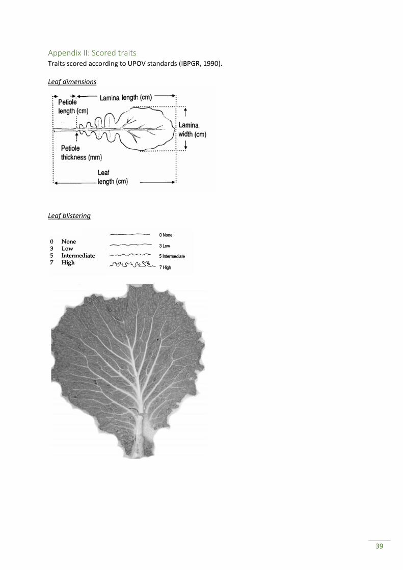
39

Appendix II: Scored traits Traits scored according to UPOV standards (IBPGR, 1990). Leaf dimensions

Leaf blistering

40

Appendix III: Karyotype Brassica genome SNP marker density distributed over the genome.

41

Appendix IV: Morphotypes tested 96-well plate with 10µL DNA isolate from the mentioned morphotypes.

1 2 3 4 5 6 7 8 9 10 11 12

A

Red cabbage

NA Chinese kale

Brussels sprout

Brussels sprout

Savoy cabbage

Brussels sprout

Broccoli White cabbage

Savoy cabbage

Kohlrabi White cabbage

B White cabbage

White cabbage

Brussels sprout

Savoy cabbage

Red cabbage

NA Brussels sprout

Winter White cabbage

Savoy cabbage

White cabbage

White cabbage

C Kale White cabbage

Borecole White cabbage

Brussels sprout

Savoy cabbage

Brussels sprout

Tronchuda cabbage

Pointed cabbage

White cabbage

Red cabbage

Cauliflower

D White cabbage

Kohlrabi White cabbage

Collards Kohlrabi Savoy cabbage

Broccoli NA Pointed cabbage

Cauliflower Savoy cabbage

Cauliflower

E Brussels sprout

White cabbage

Brussels sprout

Brussels sprout

White cabbage

White cabbage

calabrese Tronchuda cabbage

Savoy cabbage

Cauliflower Savoy cabbage

Cauliflower

F Borecole White cabbage

Brussels sprout

Brussels sprout

Kohlrabi White cabbage

calabrese Brussels sprout

Savoy cabbage

Kohlrabi Savoy cabbage

Cauliflower

G NA insularis Kohlrabi White cabbage

Kohlrabi White cabbage

Broccoli Brussels sprout

Savoy cabbage

Kohlrabi Savoy cabbage

Cauliflower

H Red cabbage

White cabbage

Savoy cabbage

Savoy cabbage

gravinae Brussels sprout

Broccoli White cabbage

Savoy cabbage

Kohlrabi White cabbage

Cauliflower

42

Appendix V: Protocols Protocols used during this study, first PCR, then restriction enzyme and the agrose gel. PCR reaction Making a PCR mastermix (this is a mix of: primers, dNTP’s, Taq buffer, Taq polymerase and MilliQ) Get a bucket or tray with ice and work on ice the entire time. Get the next solutions from the -20. Primers (forward and reverse) dNTP’s Super Taq buffer 10X Super Taq (polymerase) Place the Super Taq (polymerase) immediately on ice. Get a new Eppendorf tube and clearly write down mastermix on it. When the solutions are thawing make the calculations for the mastermix in your lab journal. This reaction will be used for 3 µl DNA sample Mastermix 1X

o Primer forward (5 pMol) 1.0 o Primer reverse (5pMol) 1.0 o dNTP’s (20 mM) 0.4 o Dream Taq buffer 10X 1.0 o Dream Taq (polymerase) 0.1 o MilliQ 5.5 o DNA (5-100 ng/ul) 1.0

Total 10.0 µl Put 10 µl of the mastermix inside a well of a PCR plate. DNA template and MilliQ are variable; increasing the amount of DNA with 1.0 µl (4.0) will decrease the amount of MilliQ with 1.0 µl (15.3 µl). When changing the volume of the MilliQ and DNA the mastermix volume changes to so in this example to 9.0 µl. (Sometimes you will need more DNA for a PCR reaction because otherwise the reaction will not work). The total volume inside a well of a PCR plate is 10 µl. Heat seal the plate with a seal next to the sealing machine (check the seal white side up). PCR machine There are two options for using the PCR machine - Use an already existing PCR program - Edit an existing program Using a program that is already stored in a machine is easy just select the program fill in your total volume of a PCR plate well and run the program There are three PCR machines 1, 2 and 3 with the files for all the Brassica programs ice machine room No. 1.159

43

Edit an existing program is easy for some machines, but some machines are difficult to program. Ask when you are not sure! Always check your program before starting the machine

Put the solutions back to the -20C freezer Start making a gel to check your products. Standard PCR program 1 cycle 94°C 3 minutes 32 cycles 94°C ½ minute 55°C ½ minute

72°C 1 minute 1 cycle 72°C 7 minutes Hold 10°C ∞ Number of cycles and annealing temperature varies, IT depends on primer design and how much DNA is added to the mastermix. CAPS protocol The enzymes are kept at -20 C and when used should be on ice all the time to prevent loss of activity. Before using check the buffer requirement depending on the lid color, the temperature for the restriction enzyme incubation may also vary, from 37 to 65 C. The incubation may be 3 hours or overnight. Mix PCR product 10µl Enzyme check units 1 unit per reaction 10x Buffer 1,5µL MQ x µL Total 15µL Mix thoroughly all the components and then distribute in the wells. Prepare a 1,5-2% gel and run no less than 2 hours. Agarose gels Safety precautions before starting… Always wear a lab coat Wear the special “blue gloves” they are made of a special nitrile material that will protect you. Check the quality of the buffer tank, if is not transparent do not hesitate in changing it, it will improve the quality of your run. Decide which kind of buffer you will use TBE or TAE, the latter is ONLY if you want to cut the PCR fragment from your gel. (see cloning section) How to prepare a gel Depending on the size of your tray you will use a different amount of buffer.

44

Size Buffer

Small 70ml

Medium 150ml

Large 300ml

After measuring the buffer, you can put it in different size bottles just make sure it is not full. For the agarose powder you will first need to define the percentage, to check DNA you should use 1% agarose, (for example if you have 100 ml of buffer you will weight 1g of agarose), to check PCR products the percentage is between 1.5 and 2%. Once you put the agarose powder in the buffer the next step is to dissolve it, you will make use of a microwave for this purpose, and after placing the bottle inside the microwave push the …button 4 times until is around 2 minutes, depending on the amount of buffer and the agarose percentage this may vary. After 2 minutes move the bottle in a circular manner, in most cases the agarose won’t be yet dissolved, put it back again in the microwave and push again for 2 more minutes. WARNING at this point the mix will begin to bubble so you have to check it constantly! After the mix is completely transparent, put an aluminum foil on top and place it in the 65 C water bath until used.

The storage at 65C step is always necessary at least for 15 minutes to cool down the mix. How to prepare the tray Select the small, medium or large tray depending on how many samples you have, the small one can be good for 10 samples, the medium one can hold more depending on the combs you use, the same for the large size. Decide which comb to use, check the width and length of the tooth, depending on how many samples and how much you want to load this may vary. Suggestion: if you want to see defined and separate bands which differ little on size go for the wide and thin tooth that can support up to 15ul. After cleaning the tray, put tape in both sides to prevent the agarose from leaking, place the holders on the large tray with the flat side inside. If you prefer place the combs at this point or after pouring the gel. Pouring the gel Check that the agarose has cooled down and put the ethidium bromide (EtBr), follow the instructions on the bottle, i.e. 1ul of EtBr per 100ml. Pour the gel carefully in the tray, check that no bubbles are formed otherwise use a tip to eliminate them. Leave the gel to solidify up to 30 minutes when it will be ready to use. How to run the gel Place your tray in the buffer tank and make sure you have enough buffer to cover the gel and up to the tank max sign After loading your samples put 5 ul of the size ladder, if is over you can get one in the stock drawer. Turn on the power supply, select a volt of 100, this may vary depending on the size of your gel and the time available. How to prepare the samples

45

For PCR products you can mix first 3ul of MQ water + 2ul of the orange loading buffer+5ul of your samples (in that order), you can also put the loading buffer directly in the PCR well (this may be dangerous if your product concentration is too high and you have many bands with small size difference).

46

Appendix VI: ANOVA Statistical analysis of all traits to check if there is a block effect.

Leaf Area Source d.f. s.s. m.s. v.r. F pr.

Block 1 3.41E+10 34053823248 39.2 < 0.001

TKI_number 822 8.86E+12 10784397797 12.42 < 0.001

Residual 2990 2.60E+12 868613243

Total 3813 1.15E+13 3014944245

Lamina Length Source d.f. s.s. m.s. v.r. F pr.

Block 1 110186 110186 14.83 < 0.001

TKI_number 822 37718969 45887 6.18 < 0.001

Residual 2990 22214514 7430

Total 3813 60043669 15747

Lamina Width Source d.f. s.s. m.s. v.r. F pr.

Block 1 317129 317129 75.29 < 0.001

TKI_number 822 93665972 113949 27.05 < 0.001

Residual 2990 12594418 4212

Total 3813 106577520 27951

Petiole Area Source d.f. s.s. m.s. v.r. F pr.

Block 1 3.03E+12 3.03E+12 19.39 < 0.001

TKI_number 822 2.70E+14 3.29E+11 2.1 < 0.001

Residual 2990 4.68E+14 1.56E+11

Total 3813 7.41E+14 1.94E+11

Petiole Length Source d.f. s.s. m.s. v.r. F pr.

Block 1 73486 73486 10.3 0.001

TKI_number 822 14728064 17917 2.5 <.001

Residual 2991 21406345 7157

Total 3813 36134409

Petiole Width Source d.f. s.s. m.s. v.r. F pr.

Block 1 140566 140566 30.04 < 0.001

TKI_number 822 14670867 17848 3.81 < 0.001

Residual 2990 13989989 4679

Total 3813 28801423 7553

Blistering Source d.f. s.s. m.s. v.r. F pr.

Block 1 33.36585 33.36585 19.49 < 0.001

TKI_number 778 4140.001 5.321338 3.108 < 0.001

Residual 778 1331.634 1.711612

Total 1557 5505.001 3.535646

47

Head Weight Source d.f. s.s. m.s. v.r. F pr.

Block 1 121187.0681 121187.0681 0.454 < 0.001

TKI_number 188 119149185.7 633772.2645 2.374 < 0.001

Residual 188 50179357.52 266911.4762

Total 377 169449730.3 449468.7807

48

Appendix VII Q-Q plots Statistical analysis if the normality assumption is uphold.

49

50

Appendix VIII: Candidate markers Allelic composition of the candidate markers for blistering and head weight.

Blistering

51

52

Head weight

53

54

Appendix IX: Candidate genes All candidate genes found in the candidate regions.

Blistering

Marker Gene Location

C03 16946055 At1g53310 C03: 16901852 : 16907280

C03 16946055 POPTR_0001s40320g C03: 16907712 : 16909983

C03 16946055 Park7 C03: 16911810 : 16913847

C03 16946055 MORF8 C03: 16914918 : 16916596

C03 16946055 27.t00109 C03: 16924322 : 16924564

C03 16946055 - C03: 16924615 : 16926230

C03 16946055 TCP4 C03: 16936104 : 16937318

C03 16946055 - C03: 16939323 : 16940000

C03 16946055 RAB11B C03: 16944092 : 16944998

C03 16946055 rnf44 C03: 16945268 : 16946967

C03 16946055 27.t00116 C03: 16957089 : 16958645

C03 16946055 RTN4IP1 C03: 16968100 : 16970099

C03 16946055 YTA7 C03: 16970782 : 16977198

C03 16946055 - C03: 16979954 : 16980440

C03 16946055 PCMP-H86 C03: 16989146 : 16991200

C04 20520782 SPL3 C04: 20510435 : 20510961

C04 20520782 DRMH1 C04: 20513498 : 20514035

C04 20520782 FES1 C04: 20519125 : 20521697

C04 20520782 At4g28440 C04: 20523292 : 20524027

C04 20520782 At2g33847 C04: 20524717 : 20525511

C04 20520782 ARF3 C04: 20533558 : 20536202

C04 34477381 P20 C04: 34451185 : 34451733

C04 34477381 At2g32040 C04: 34457383 : 34459514

C04 34477381 RPS12C C04: 34461316 : 34462565

C04 34477381 CAF1-7 C04: 34463330 : 34464145

C04 34477381 27.t00096 C04: 34469855 : 34470058

C04 34477381 CAF1-7 C04: 34476766 : 34477596

C04 34477381 PURA1 C04: 34478663 : 34480154

C04 34477381 glo1 C04: 34481199 : 34482163

C04 34477381 OFP16 C04: 34484983 : 34485693

C04 34477381 HSP70-8 C04: 34493683 : 34495374

C04 34477381 SDT1 C04: 34514002 : 34515475

C04 34477381 40.t00015 C04: 34519807 : 34520406

C05 10319967 - C05: 10296060 : 10296599

C05 10319967 COBL11 C05: 10297411 : 10298221

C05 10319967 27.t00116 C05: 10301087 : 10304217

C05 10319967 HSFA1D C05: 10307772 : 10310592

C05 10319967 ATPK2 C05: 10314833 : 10315177

C05 10319967 lepA C05: 10316716 : 10317092

C05 10319967 SYP22 C05: 10318025 : 10319846

C05 10319967 F5D14.2 C05: 10320230 : 10321123

55

C06 18873634 - -

C07 5829451 At2g04480 C07: 5799245 : 5799778

C07 5829451 75-1-127BAC12.1 C07: 5862153 : 5863381

C08 14790421 MAP2B C08: 14821877 : 14823705

Head weight

Marker Gene Location

C01_33540674 & C01_33540749 IAA19 C01: 33575783 : 33576943

C01_33540674 & C01_33540750 F14P13.5 C01: 33549224 : 33550864

C01_33540674 & C01_33540751 At1g28030 C01: 33544774 : 33546291

C01_33540674 & C01_33540752 At3g15550 C01: 33538980 : 33541699

C01_33540674 & C01_33540753 At1g52740 C01: 33537766 : 33538430

C01_33540674 & C01_33540754 UVR3 C01: 33534570 : 33537294

C08_31561734 AIR12 C08: 31604539 : 31605837

C08_31561734 At3g59040 C08: 31590046 : 31596823

C08_31561734 PME35 C08: 31567374 : 31567961

C08_31561734 PME35 C08: 31565252 : 31565911

C08_31561734 LPE10 C08: 31561508 : 31563156

C08_31561734 PAR2 C08: 31548318 : 31548644

C08_31561734 GAUT8 C08: 31533425 : 31537356

C08_31561734 ARALYDRAFT_486331 C08: 31517070 : 31523233

C08_31561734 ARALYDRAFT_348948 C08: 31541893 : 31542924

C08_31561734 At3g58930 C08: 31556359 : 31557423

C09_12411624 T27D20.13 C09: 12401012 : 12403161

C09_12411624 ISU3 C09: 12408536 : 12409714

C09_12411624 PFP-BETA C09: 12412689 : 12416219

C09_12411624 PAP1 C09: 12427433 : 12433563

C09_12411624 At1g05000 C09: 12447375 : 12448677

C09_12411624 WDL2 C09: 12453586 : 12455300

C09_27943876 & C09_27943899 & C09_27943857 NEDP1 C09: 27984427 : 27984882

C09_27943876 & C09_27943899 & C09_27943858 APUM19 C09: 27967024 : 27967566

C09_27943876 & C09_27943899 & C09_27943859 - C09: 27954829 : 27965410

C09_27943876 & C09_27943899 & C09_27943860 At5g60142 C09: 27953146 : 27954087

C09_27943876 & C09_27943899 & C09_27943861 At5g60130 C09: 27950431 : 27951551

C09_27943876 & C09_27943899 & C09_27943862 TOE2 C09: 27946639 : 27949476

C09_27943876 & C09_27943899 & C09_27943863 40.t00055 C09: 27919853 : 27920440

C09_27943876 & C09_27943899 & C09_27943864 APRR3 C09: 27914944 : 27917092

C09_27943876 & C09_27943899 & C09_27943865 MGO3.6 C09: 27913604 : 27914076

C09_27943876 & C09_27943899 & C09_27943866 RDR3 C09: 27910937 : 27912192

C09_27943876 & C09_27943899 & C09_27943867 RDR4 C09: 27903104 : 27903673

C09_36633552 At5g11090 C09: 36591314 : 36591979

C09_36633552 80A08_24 C09: 36599961 : 36601020

C09_36633552 At1g53530 C09: 36604859 : 36605641

C09_36633552 At5g11070 C09: 36610591 : 36611040

C09_36633552 TRAPPC9 C09: 36614524 : 36619298

56

C09_36633552 ALF4 C09: 36619657 : 36623336

C09_36633552 PBS1 C09: 36625120 : 36627557

C09_36633552 At5g11010 C09: 36628375 : 36630678

C09_36633552 At5g11000 C09: 36632977 : 36634140

C09_36633552 ARG7 C09: 36636473 : 36636919

C09_36633552 ZFP3 C09: 36642009 : 36642737

C09_36633552 CAF1-10 C09: 36648823 : 36649665

C09_36633552 ALTERED SEED GERMINATION 2 C09: 36662215 : 36666644

C09_36633552 CIPK5 C09: 36671931 : 36673229