arX

iv:0

708.

0883

v1 [

gr-q

c] 7

Aug

200

7

The complete LQG propagator

I. Difficulties with the Barrett-Crane vertex

Emanuele Alesciab, Carlo Rovellib

a Dipartimento di Fisica Universita di Roma Tre, I-00146 Roma EUbCentre de Physique Theorique de Luminy∗, Universite de la Mediterranee, F-13288 Marseille EU

June 14, 2013

Abstract

Some components of the graviton two-point function have been recently computed in the context

of loop quantum gravity, using the spinfoam Barrett-Crane vertex. We complete the calculation of

the remaining components. We find that, under our assumptions, the Barrett-Crane vertex does

not yield the correct long distance limit. We argue that the problem is general and can be traced

to the intertwiner-independence of the Barrett-Crane vertex, and therefore to the well-known

mismatch between the Barrett-Crane formalism and the standard canonical spin networks. In a

companion paper we illustrate the asymptotic behavior of a vertex amplitude that can correct

this difficulty.

1 Introduction

A key problem in loop quantum gravity (LQG) [1, 2, 3] is to derive low–energy quantities from thefull background independent theory. A strategy for addressing this problem was presented in [4] andsome components of the graviton propagator of linearized quantum general relativity

Gabcd(x, y) =⟨

0|hab(x)hcd(y)|0⟩

(1)

(hab(x), a, b = 1, ...4, is the linearized gravitational field) were computed in [5] (at first order) and [6](to higher order) starting from the background-independent theory and using a suitable expansion.More precisely, the “diagonal” components Gaacc(x, y) have been computed in the large-distance limit.This result has been extended to the three-dimensional theory in [7]; an improved form of the boundarystates used in the calculation has been considered in [8]; and the exploration of some Planck-lengthcorrections to the propagator of the linear theory has begun in [9]. See also [10].

Here we complete the calculation of the propagator. We compute the nondiagonal terms ofGabcd(x, y), those where a 6= b or c 6= d, and therefore derive the full tensorial structure of thepropagator. The nondiagonal terms are important because they involve the intertwiners of the spinnetworks. Avoiding the complications given by the intertwiners’ algebra was indeed the rationalbehind the relative simplicity of the diagonal terms.

The dependence of the vertex from the intertwiners is a crucial aspect of the definition of thequantum dynamics. The particular version of the dynamics used in [5] and [6], indeed, is defined

∗Unite mixte de recherche (UMR 6207) du CNRS et des Universites de Provence (Aix-Marseille I), de la Mediterranee(Aix-Marseille II) et du Sud (Toulon-Var); laboratoire affilie a la FRUMAM (FR 2291).

1

by the Barrett-Crane (BC) vertex [11], where the dependence on the intertwiners is trivial. This isan aspect of the BC dynamics that has long been seen as suspicious (see for instance [12]); and it isdirectly tested here.

We find that under our assumptions the BC vertex fails to give the correct tensorial structure ofthe propagator in the large-distance limit. We argue that this result is general, and cannot be easilycorrected, say by a different boundary state. This result is of interest for a number of reasons. First,it indicates that the propagator calculations are nontrivial; in particular they are not governed just bydimensional analysis, as one might have worried, and they do test the dynamics of the theory. Second,it reinforces the expectation that the BC model fails to yield classical GR in the long-distance limit.Finally, and more importantly, it opens the possibility of studying the conditions that an alternativevertex must satisfy, in order to yield the correct long-distance behavior. This analysis is presented inthe companion paper [13].

The BC model exists in a number of variants [2, 14]; the results presented here are valid for all ofthem. Alternative models have been considered, see for instance [15]. Recently, a vertex amplitudethat modifies the BC amplitude, and which addresses precisely the problems that we find here, hasbeen proposed [16, 17], see also [18]. It would be of great interest to repeat the calculation presentedhere for the new vertex proposed in those papers.

This paper is organized as follows. In section 2 we formulate the problem and we compute theaction of the field operators on the intertwiner spaces. This calculation is a technical result with aninterest in itself. Here we will use only part of this result, the rest will be relevant for the companionpaper. In section 3 we discuss the form of the boundary state needed to describe a semiclassicalgeometry to the desired approximation. Section 4 contains the main calculation. In Section 5 wediscuss the interpretation of our result.

This paper is not self-contained: for full background, see [6]. For an introduction to the generalideas and the formalism, see the book [2]. However, we include here a detailed Appendix, with allbasic equations of the recoupling theory needed for the calculations. The Appendix corrects someimprecisions in previous formularies and can be useful as a tool for further developments. We workentirely in the euclidean theory.

2 The propagator in LQG

We refer to [6] for the notation and the basic definitions. We want to compute

Gabcdq (x, y) = 〈W |hab(x) hcd(y)|Ψq〉 (2)

to first order in λ. Here Ψq is a state peaked on q, which is the (intrinsic and extrinsic) 3d geometryof the boundary of a spherical 4-ball of radius L in R4, x and y are two points in this geometry, ab aretangent indices at x and cd tangent indices at y in this geometry. That is, Gabcd

q (x, y) is a quantitythat transforms covariantly under 3d diffeomorphisms acting conjointly on x, y, on the indices abcd,and on q. hab(x) is the fluctuation of the gravitational field over the euclidean metric. W is theboundary functional, that defines the dynamics; it is assumed to be given here by a Barrett-CraneGFT [14, 24] with coupling constant λ. The expansion parameter λ is a cut-off in the degrees offreedom of wavelength smaller than L. Degrees of freedom of wavelength larger than L do not enterthe problem. We normalize here Ψq by 〈W |Ψq〉 = 1.

Consider the s-knot (abstract spin network) basis |s〉 = |Γ, j, i〉, where Γ is an abstract graph,n, m... label the nodes of Γ, j = {jmn} are the spins and i = {in} the intertwiners of a spin networkwith graph Γ. Insert a resolution of the identity in (2)

Gabcdq (x, y) =

∑

s

〈W |s〉〈s|hab(x) hcd(y)|Ψq〉. (3)

2

To first order in λ, 〈W |s〉 = W [s] = W [Γ, j, i] is different from zero only if Γ is the pentagonal graph,that is, for the s-knot

s =

q

qq

q

q ✄✄✄✄✄

◗◗

◗◗✑✑

✑✑

❈❈❈❈❈

❇❇❇

❧❧

✂✂✂✂✂

✂✂❇

❇❇❇

✚✚✚

★★

★★

❝❝

❝❝

i1

i2

i3

i5

i4

j12

j23

j34

j45

j51

j13j35

j14j24

j52. (4)

In this case, and from now on, we have five intertwiners i = {in}, labeled by n, m, ... = 1, ..., 5 andten spins j = {jmn}. We use equally the indices i, j, k, ... = 1, ..., 5 to indicate the nodes. Since theoperators hab(x) do not change the graph (they are operators acting on the spin and intertwinersvariables j, i)

Gabcdq (x, y) =

∑

j,i

W (j, i) hab(x)hcd(y)Ψ(j, i) (5)

where W (j, i) = W [Γ5, j, i] and Ψ(j, i) = Ψq[Γ5, j, i] = 〈Γ5, j, i|Ψq〉, and the sum is over the fifteenvariables (j, i) = (jnm, in). (We use the physicists notation hcd(y)Ψ(j, i) for [hcd(y)Ψ](j, i).)

Following [6], we choose the form of Ψ(j, i) by identifying Γ5 with the dual skeleton of a regulartriangulation of the three-sphere. Each node n = 1, ..., 5 corresponds to a tetrahedron t1....t5 and wechoose the points x and y to be the centers xn and xm of the two tetrahedra tn and tm. We consider

Gij,kl

q n,m := Gabcdq (xn, xm) n(ni)

a n(nj)

b n(mk)

c n(ml)

d , (6)

where n(ij)a is the one–form normal to the triangle that bounds the tetrahedra ti and tj . From now

on, we assume n 6= m. Since hab = gab − δab = EaiEbi − δab, this is given by

Gij,kl

q n,m = 〈W |(

E(ni)

n · E(nj)

n − n(ni) · n(nj))(

E(mk)

m · E(ml)

m − n(mk) · n(ml))

|Ψq〉=

∑

j,i

W (j, i)(

E(ni)

n · E(nj)

n − n(ni)· n(nj))(

E(mk)

m · E(ml)

m − n(mk)· n(ml))

Ψ(j, i). (7)

where, E(ml)n = Ea(~x)n(ml)

a is valued in the su(2) algebra and, with abuse of notation, the scalarproduct between the triad fields indicates the product in the su(2) algebra (in the internal space);while the scalar product among the one forms n(ij) is the one defined by the background metric δab.In the rest of the paper, we compute the right hand side of (7).

2.1 Linearity conditions

Before proceedings to the actual computation of (7), let us pause to consider the following question.The four normal one-forms of a tetrahedron sum up to zero. Thus

∑

i6=n

n(ni)

a = 0. (8)

This determines a set of linear conditions that must be satisfied by Gij,kl

q n,m. In fact, from the lastequation it follows immediately that

∑

i6=n

Gij,kl

q n,m = 0. (9)

(The existence of conditions of this kind, of course, is necessary, since the four one forms n(ni)a (for

fixed n) span a three-dimensional space, namely the space tangent to the boundary surface at xn,

3

and therefore the quantities Gij,kl

q n,m are determined by the restriction of the bi-tensor Gabcdq to these

tangent spaces.) How is it possible that the linear conditions (9) are satisfied by the expression (7)?The answer is interesting. The operator E(ni)

n · E(nj)n acts on the space of the intertwiners of

the node n. This is the SU(2) invariant part of the tensor product of the four SU(2) irreduciblerepresentations determined by the four spins jni. In particular, E(ni)

n is the generator of SU(2)rotations in the representation jni. Therefore

J =∑

i6=n

E(ni)

n (10)

is the generator of SU(2) rotations in the tensor product of these representations. But the intertwinersspace is precisely the SU(2) invariant part of the tensor product. Therefore J = 0 on the intertwinerspace. Inserting this in (7), equation (9) follows immediately. Therefore the linearity conditions be-tween the projections of the propagator in the space tangent to the boundary surface are implementedby the SU(2) invariance at the nodes.

2.2 Operators

We begin by computing the action of the field operator E(ni)n · E(nj)

n on the state. This operator actson the intertwiner space at the node n. It acts as a “double grasping” [3] operator that inserts avirtual link (in the spin-one representation) at the node, connecting the links labelled ni and nj. Thestate of each node n (n = 1, .., 5) is determined by five quantum numbers: the four spins jnj (n 6= j,j = 1, .., 5) that label the links adjacent to the node and a quantum number in of the virtual link thatspecifies the value of the intertwiner. In this section we study the action of this operator on a singlenode n; hence we drop for clarity the index n and write the intertwiner quantum number as i, theadjacent spins as ji, jj , jp, jq, and the operator as E(i) · E(j). We use the graphic notation of SU(2)recoupling theory to compute the action of the operators on the spin network states (see [2]). Thebasics of this notation are given in Appendix A and the details of the derivation of the action of theoperator are given in Appendix C. Choose a given pairing at the node, say (i, j)(p, q) (and fix theorientation, say clockwise, of each of the two trivalent vertices). We represent the node in the form

i =

jj

ji

jp

jq

�❅ �

❅

ir r

,

(11)

where we use the same notation i for the intertwiner and the spin of the virtual link that determinesit. This basis diagonalizes the operator E(i) ·E(j), but not the operators E(i) ·E(q) and E(i) ·E(p). Weconsider the action of these three “doublegrasping” operator on this basis. The simplest is the actionof E(i) · E(i). Using the formulas in Appendix C we have easily

E(i) · E(i)

∣

∣

∣

∣

∣

∣

∣jj

ji

jp

jq

�❅ �

❅

ir r

⟩

= −(N i)2

∣

∣

∣

∣

∣

∣

∣jj

ji

jp

jqr

r

��

❅❅ �

�

❅❅

i1

r r

⟩

= Cii

∣

∣

∣

∣

∣

∣

∣jj

ji

jp

jq

�❅ �

❅

ir r

⟩

, (12)

whereCii = C2(ji). (13)

with C2(a) = a(a + 1) is the Casimir of the representation a. Just slightly more complicated is theaction of E(i) · E(j)

E(i) · E(j)

∣

∣

∣

∣

∣

∣

∣jj

ji

jp

jq

�❅ �

❅

ir r

⟩

= −N iN j

∣

∣

∣

∣

∣

∣

∣jj

ji

jp

jqr

r

��

❅❅ �

�

❅❅

i1 r r

⟩

= Dij

∣

∣

∣

∣

∣

∣

∣jj

ji

jp

jq

�❅ �

❅

ir r

⟩

, (14)

4

where

Dij =C2(i) − C2(ji) − C2(jj)

2. (15)

In these two cases the action of the operator is diagonal. If, instead, the grasped links are notpaired together, the action of the operator is not diagonal in this basis. In this case, the recouplingtheory in the Appendix gives

E(i) · E(q)

∣

∣

∣

∣

∣

∣

∣jj

ji

jp

jq

�❅ �

❅

ir r

⟩

= −N iN q

∣

∣

∣

∣

∣

∣

∣jj

ji

jp

jqr r

��

❅❅ �

�

❅❅

i

1

r r

⟩

=

= X iq

∣

∣

∣

∣

∣

∣

∣jj

ji

jp

jq

�❅ �

❅

ir r

⟩

− Y iq

∣

∣

∣

∣

∣

∣

∣jj

ji

jp

jq

�❅ �

❅

i − 1r r

⟩

− Ziq

∣

∣

∣

∣

∣

∣

∣jj

ji

jp

jq

�❅ �

❅

i + 1r r

⟩

,

(16)

where

X iq = −(

C2(i) + C2(ji) − C2(jj)) (

C2(i) + C2(jq) − C2(jp))

4 C2(i), (17)

Y iq = − 1

4i dim(i)

√

(ji + jj + i + 1)(ji − jj + i)(−ji + jj + i)(ji + jj − i + 1) ·

·√

(jp + jq + i + 1)(jp − jq + i)(−jp + jq + i)(jp + jq − i + 1),

(18)

Ziq = − 1

4(i + 1) dim(i)

√

(ji + jj + i + 2)(ji − jj + i + 1)(−ji + jj + i + 1)(ji + jj − i) ·

·√

(jp + jq + i + 2)(jp − jq + i + 1)(−jp + jq + i + 1)(jp + jq − i).

(19)

The last possibility is

E(i) · E(p)

∣

∣

∣

∣

∣

∣

∣jj

ji

jp

jq

�❅ �

❅

ir r

⟩

= −N iNp

∣

∣

∣

∣

∣

∣

∣jj

ji

jp

jqr

r

��

❅❅ �

�

❅❅

ir r

⟩

=

= X ip

∣

∣

∣

∣

∣

∣

∣jj

ji

jp

jq

�❅ �

❅

ir r

⟩

+ Y ip

∣

∣

∣

∣

∣

∣

∣jj

ji

jp

jq

�❅ �

❅

i − 1r r

⟩

+ Zip

∣

∣

∣

∣

∣

∣

∣jj

ji

jp

jq

�❅ �

❅

i + 1r r

⟩

.

(20)

Note that X ip is exactly X iq with p and q switched and Y ip = Y iq, Zip = Ziq.Finally, we have to take care of the orientation. As shown in the Appendix, the sign of the non

diagonal terms is influenced by the orientations: in the planar representation that we are using, thereis a + sign if the added link intersect the virtual one and a −1 otherwise.

Summarizing, in a different notation and reinserting explicitly the index n of the node, we have thefollowing action of the EE operators. If the grasped links are paired together we have the diagonalaction

E(ni) · E(nj)|Γ5, j, i1, .., in, .., i5〉 = Sij

n |Γ5, j, i1, .., in, .., i5〉, (21)

where

Sij

n =

{

Cii = C2(jni) if i = j,

Dij =C2(in)−C2(jni)−C2(jnj)

2 if i 6= j.(22)

5

If the grasped links are not paired together, we have the non-diagonal action

E(ni) · E(nq)|Γ5, j, i1, .., in, .., i5〉 =

=

X iq

n |Γ5, j, i1, .., in, .., i5〉 + Y iq

n |Γ5, j, i1, .., in−1, .., i5〉+Ziq

n |Γ5, j, i1, .., in+1, .., i5〉 if i opposite to q,

X iq

n |Γ5, j, i1, .., i, .., i5〉 − Y iq

n |Γ5, j, i1, .., in−1, .., i5〉−Ziq

n |Γ5, j, i1, .., in+1, .., i5〉 otherwise.

(23)

This completes the calculation of the action of the gravitational field operators.

3 The boundary state

The boundary state utilized in [6] was assumed to have a gaussian dependence on the spins, and tobe peaked on a particular intertwiner. This intertwiner was assumed to project trivially onto the BCintertwiner of the BC vertex. This was a simplifying assumption permitting to avoid dealing with theintertwiners, motivated by the fact that intertwiners play no role for the diagonal terms. However, itwas also pointed out in [6] that this procedure is not well defined, because of the mismatch betweenSO(4) linearity and SU(2) linearity (see the discussion in the Appendix of [6]). Here we face theproblem squarely, and consider the intertwiner dependence of the boundary state explicitly.

A natural generalization of the gaussian state used in [6], whith a well-defined and non-trivialintertwiner dependence, is the state

Φ(j, i) = C exp

{

− 1

2j0

∑

(ij)(mr)

α(ij)(mr) (jij − j0)(jmr − j0) + iΦ∑

(ij)

jij

}

·

· exp

−∑

n

(in − i0)2

4σ+∑

p6=n

φ(jnp − j0)(in − i0) + iχ(in − i0)

(24)

The first line of this equation is precisely the spin dependence of the state used in [6]. The second linecontains a gaussian dependence on the intertwiner variables. More precisely, it includes a diagonalgaussian term, a nondiagonal gaussian spin-intertwiner term, and a phase factor. We do not includenon-diagonal intertwiner-intertwiner terms here. These will be considered in the companion paper.

Let us fix some of the constants appearing in (24), by requiring the state to be peaked on theexpected geometry. The constant j0 determines the background area A0 of the faces, via C(jnm) =Anm. As in [6], we leave j0 free to determine the overall scale. The constant Φ determines thebackground values of the angles between the normals to the tetrahedra. As in [6], we fix them tothose of a regular four-simplex, namely cosΦ = −1/4.

The constant i0 is the background value of the intertwiner variable. As shown in [6], the spin ofthe virtual link in is the quantum number of the angle between the normals of two triangles. Moreprecisely, the Casimir C(in) of the representation in is the operator corresponding to the classicalquantity

C2(in) = Ani + Anj + 2 ~n(ni) · ~n(nj), (25)

where i and j are the paired links at the node n and Ani is the area of the triangle dual to the link(ni). The scalar product of the normals to the triangles can therefore be related to the Casimirs ofspins and intertwiners:

n(ni) · n(nj) =C(in) − C(jni) − C(jnj)

2. (26)

For each node, the state must therefore be peaked on a value i0 such that

i0(i0 + 1) = A0 + A0 + 2A0A0 cos θij , (27)

6

where cos θij is the 3d dihedral angle between the faces of the tetrahedron. For the regular 4-symplex,in the large distance limit we have Aij = j0, cos θij = − 1

3 , which gives

i0 =2√3

j0. (28)

This fixes i0. Notice that in [6] equation (25) refers to the Casimir of an SO(4) simple representationand follows from the quantization of the Plebanski 2 form BIJ = eI∧eJ associated with the discretizedgeometry. Exactly the same result follows from equation (14) directly from LQG.

Fixing i0 in this manner determines only the mean value of the angle θij between the two trianglesthat are paired together in the chosen pairing. What about the mean value of the angles betweenfaces that are not paired together, such as θiq? It is shown in [20] that a state of the form e(i−i0)2/σ

is peaked on θiq = 0, which is not what we want; but the mean value of θiq , can be modified byadding a phase to the state. This is the analog of the fact that a phase changes the mean value of themomentum of the wave packet of a non relativistic particle, without affecting the mean value of theposition. In particular, it was shown in [20] that by choosing the phase and the width of the Gaussianto be

χ =π

2, σ =

j03

, (29)

we obtain a state whose mean value and variance for all angles is the same.Let us therefore adopt here these values. Still, the present situation is more complicated than the

case considered in [20], because the tetrahedron considered there had fixed and equal values of theexternal spins; while here the spins can take arbitrary values around the peak symmetric configurationjnm = j0. As a consequence, when repeating the calculation in [20], one finds additional spin-intertwiner gaussian terms. These, however can be corrected by fixing the spin-intertwiner gaussianterms in (24). A detailed calculation (see below), shows indeed that in the large j0 limit, the state(24) transforms under change of pairing into a state with the same intertwiner mean value and thesame variance σ, provided we also choose

φ = −i3

4j0, (30)

which we assume from now on. With these values and introducing the difference variables δin = in−i0and δjmr = jmr − j0 the wave functional, given in (24), reads

Φ(j, i) = C e−1

2j0

P

α(ij)(mr)δjijδjmr+iΦP

ij δjij e−P

n

„

3(δin)2

4j0−i“

P

a3

4j0δjan−π

2

”

δin

«

. (31)

This state, however, presents a problem, which we discuss in the next section.

3.1 Pairing independence

It is natural to require that the state respects the symmetries of the problem. A moment of reflectionshows that the state (31) does not. The reason is that the variables in are the spin of the virtual linksin one specific pairing, and this breaks the symmetry of the four-simplex. The phases and varianceschosen assure that the mean values are the desired ones, hence symmetric; but an explicit calculationconfirms that the relative fluctuations of the angle variables determined by the state (31) depend onthe pair chosen.

To correct the problem, recall that there are three natural bases in each intertwiner space, deter-mined by the three possible pairings of these links. Denote them as follows.

ix =

jj

ji

jp

jq

�❅ �

❅

ixr r iy =

jj

ji

jp

jq

�

❅�

❅

iyr

r

iz =

jj

ji

jp

jq

��

�❅❅

❅

izr r , (32)

7

where we conventionally denote ix ≡ i the basis in the pairing chosen as reference. These basesdiagonalize the three non commuting operators E(i) · E(j), E(i) · E(q) and E(i) · E(p), respectively.Furthermore a spin-network state is specified by the orientation of the three-valent nodes [19]; we fixthis orientation by giving an ordering to the links. We write for instance

ix(+,−) =

jj

ji

jp

jq

�❅ �

❅

ixr r

+ −(33)

where the plus sign + (-) means anticlockwise (clockwise) ordering of the links in the two nodes. Acomplete basis in the space of the spin networks on Γ5 is specified giving the pairing and the orientationat each node. In order to label the different bases, introduce at each node n a variable mn that takesthe values mn = x, y, z, namely that ranges over the three possible pairings at the node. Similarly,introduce a variables on = {(++),(+−),(−+),(−−)} that labels the possible orientations. To correct thepairing dependence of the state (24), let us first rewrite it in the notation

|Φq〉x++ =∑

j,ix++

Φ[j, ix++] |j, ix++〉. (34)

where the suffix x++ to the ket emphasizes the fact that the state has been defined with the chosenpairing and orientation at each node. We can now consider a new state obtained by summing (34)over all choices of pairings and orientations. That is, we change the definition of the boundary stateto

|Ψq〉 =∑

mn,on

|Φq〉mnon. (35)

where∑

mn,on=∑

m1...m5

∑

o1...o5and

|Φq〉mnon=

∑

j,imnon

Φ[j, imnon ] |j, imnon〉. (36)

namely |Φq〉mnonis the same as the state |Φq〉x++, but defined with a different choice of pairing at

each node.Since (by assumption) (24) does not depend on the orientation, the sum over the orientation of

the node (say) 1, in (35) reduces to a term proportional to

∑

o

|j, io1, i2, i3, i4, i5〉 ∼∣

∣

∣

∣

∣

∣

∣j12

j13

j15

j14

�❅ �

❅

i1

+ +

r r

⟩

+

∣

∣

∣

∣

∣

∣

∣j12

j13

j15

j14

�❅ �

❅

i1

+ −

r r

⟩

+

∣

∣

∣

∣

∣

∣

∣j12

j13

j15

j14

�❅ �

❅

i1

− +

r r

⟩

+

∣

∣

∣

∣

∣

∣

∣j12

j13

j15

j14

�❅ �

❅

i1

− −

r r

⟩

.

(37)

As shown in the Appendix, the change in orientation of a vertex produces the sign (−1)a+b+c, wherea, b, c are the three addiacent spins. Hence

∑

o

|j, io1, i2, i3, i4, i5〉 ∼

=(

1 + (−1)j14+j15+i1 + (−1)j12+j13+i1 + (−1)j12+j13+j14+j15+2 i1) ∣

∣j, i++1 , i2, i3, i4, i5

⟩

=

{

4∣

∣j, i++1 , i2, i3, i4, i5,

⟩

if(

j12 + j13 + im11 = 2n1 and j14 + j15 + im1

1 = 2n2

)

,

0 otherwise.

(38)

8

We can therefore trade the sum over orientations in (35) with a condition on the spins summed over:at all trivalent vertices, the sum of the two external spins and the virtual spin, must be an eveninteger. (The factor 4 is absorbed in the normalization factor C.) With this understanding, we dropthe sum over orientations in (35), which now reads

|Ψq〉 =∑

mn

|Φq〉mn, (39)

where all orientations are fixed. This state can of course also be expressed in terms of a single basis

|Ψq〉 =∑

j,i

Ψq(j, i) |j, i〉, (40)

where we have returned to the notation in = ix,++n . Its components are

Ψ(j, i) = 〈j, i|Ψq〉 =∑

mn

Φ(j, imn) 〈j, i|j, imn〉. (41)

The matrices of the change of basis 〈j, i|j, imn〉 are (products of five) 6-j Wigner-symbols, as given bystandard recoupling theory.

The state (39) is the boundary state we shall use. The complication of the sum over pairings isless serious than what could seem at first sight, due to a key technicality that we prove in the nextsection: the components of (39) become effectively orthogonal in the large distance limit.

3.1.1 Orthogonality of the terms in different bases in the large j0 limit

Suppose we want to compute the norm of the boundary state, in the limit of large j0. From (39), thisis given by

|Ψ|2 =∑

mn

∑

m′n

mn〈Φq|Φq〉m′

n (42)

We now show that in the large j0 limit the non-diagonal terms of this sum (those with mn 6= m′n)

vanish. Consider one of these terms, say

I = mn〈Φq|Φq〉m′

n=∑

jimn

∑

j′im′n

Φ(j, imn) Φ[j′, im′n ] 〈jimn |j′im′

n〉 (43)

where, say, mn = (x, x, x, x, x) and m′n = (y, x, x, x, x). The scalar product is diagonal in the spins j

and is given by 6-j symbol in the intertwiners quantum numbers. Hence

I =∑

j

∑

imn

∑

im′n

Φ(j, imn) Φ[j, im′n ] 〈ix1 |iy1〉, (44)

where (see Appendix D),

〈ix1 |iy1〉 = (−1)j13+j14+ix1+iy

1

√

dix1diy

1

{

j12 j13 ix

1

j15 j14 iy

1

}

. (45)

In the large j0 limit, this sum can be approximated by an integral, as in [6]. Both the spin and theinterwiner sums become gaussian integrals, peaked respectively on j0 and i0. The range of the sumover intertwiners is finite for finite j0, because of the Clebsh Gordan conditions at the two trivalentnode; but this range is much larger than the width of the Gaussian in the limit, and therefore the

9

integral over the intertwiner variables too can be taken over the entire real line. In the limit, the 6-jsymbol has the asymptotic value [22]

{

j12 j13 ix

1

j15 j14 iy

1

}

≈ ei(SR+ π4 ) + e−i(SR+ π

4 )

√12πV

, (46)

where SR is the Regge action of a tetrahedron with side length determined by the spins of the 6jsymbol, and V is its volume. Changing the sum into an integration and using this, we have

I =

∫

dj

∫

di

∫

diy1 Φ(j, i) Φ(j, im′n) (−1)j13+j14+ix

1+iy1

ei(SR+ π4 ) + e−i(SR+ π

4 )

√12πV

. (47)

Inserting the explicit form of the state (31) gives

I =

∫

dj

∫

di e− 1

j0

P

α(ij)(mr)δjijδjmr−P

n 6=13(δin)2

2j0− 3(δi1)2

4j0−i“

P

a3

4j0δjan−π

2

”

δix1

·∫

diy1 e− 3(δi

y1)2

4j0 ei“

P

a3

4j0δjan−π

2

”

δiy1

ei(SR+πδiy1+ π

4 ) + e−i(SR−πδiy1+ π

4 )

√12πV

.

(48)

In the limit, only the first terms in the expansion of the Regge action around the maximum ofthe peak of the Gaussian matter. We thus Taylor expand the Regge action in its six entries j1n, ix

1, iy

1

around the background values j0 and i0.

Sj [jna] =∂SR

∂j1n

∣

∣

∣

∣

j0,i0

δj1n +∂SR

∂ix

1

∣

∣

∣

∣

j0,i0

δix

1 +∂SR

∂iy

1

∣

∣

∣

∣

j0,i0

δiy

1 + higher order terms. (49)

The key point now is that the first of these terms is a rapidly oscillating phase factor in the j1n

variable. The Gaussian j1n integration in (48) is suppressed by this phase factor. More precisely, theintegral is like a Fourier transform in the j1n variable, of a gaussian centered around a large valueof j0 with variance proportional

√j0; this Fourier transform is then a gaussian with variance 1/

√j0,

which goes to zero in the j0 → ∞ limit. QED.

3.1.2 Change of basis

For later convenience, let us also give here the expression of the state (31) under the transformationinduced by the change of basis associated to a change of pairing. Say we change from the basis iy tothe basis ix in the node n = 1. Then directly from (41) we have

Φ′q[j, ix

1, i2...i5] = e− 1

2j0

P

α(ij)(mr)δjijδjmr+iP

Φδjij e−P

n 6=1

„

3(δin)2

4j0−i“

P

a3

4j0δjan−π

2

”

δin

«

·∑

iy1

e−„

3(δiy1 )2

4j0−i“

P

a3

4j0δja1−π

2

”

δiy1

«

(−1)j13+j14+ix1+iy

1

√

dix1diy

1

{

j12 j13 ix

1

j15 j14 iy

1

} (50)

where, we recall, the sum over intertwiners is under the condition (38) that that gives (−1)j13+j14+ix1 =

1 We can evaluate the sum in the large j0 limit by approximating it again with an integral. Insertingthe asymptotic expansion of the 6j symbol, we have

Φ′q(j, ix

1, i2...i5) = e− 1

2j0

P

α(ij)(mr)δjijδjmr+iP

Φδjij e−P

n 6=1

„

3(δin)2

4j0−i“

P

a3

4j0δjan−π

2

”

δin

«

eiπi0

·∫

dδiy

1e−„

3(δiy1 )2

4j0−i“

P

a3

4j0δja1−π

2

”

δiy1

«

√

dix1diy

1

ei(SR+πδiy1+π

4 ) + e−i(SR−πδiy1+ π

4 )

√12πV

.

(51)

10

This can be computed expanding the Regge action to second order around j0 and i0. As shown inthe Appendix F, the result is

Φ′q(j, ix

1, i2, ..., i5) = Φ(j, ix

1, i2, ..., i5)N1 e−iS[j1a]e−2i

“

P

a3

4j0δja1

”

δix1 , (52)

where N1 is a normalization constant with |N1|2 = 1, and S[j1a] is the expansion of the Regge Actionlinked to the tetrahedron associated with the {6j} symbol (46) up to the second order only in the linkvariables, that is

S[jna] =∂SR

∂j1n

∣

∣

∣

∣

j0,i0

δj1n +∂2SR

∂j1n∂j1n′

∣

∣

∣

∣

j0,i0

δj1nδj1n′ +1

2

∂2SR

∂2j1n

∣

∣

∣

∣

j0,i0

(δj1n)2. (53)

This result follows from the choice (29) and (30) of the parameters in (24). In particular, the value χn =

π2 makes the intertwiner phase equal, with opposite sign, to the term exp−i

(

∂SR

∂iy1

∣

∣

∣

j0,i0δiy

1 − πδiy1

)

,

namely the term in the expansion of the Regge action SR linear in the variable δiy

1. This selects oneof the two exponentials in the asymptotic expansion (46), while the rapidly oscillating phase factor inthe variables δiy1 cancels the other.

The same calculation gives the iz → ix change of variable

Φ′′q(j, ix

1, i2, ..., i5) = Φ(j, ix

1, i2, ..., i5)N1 e−iS′[j1a]e−2i

“

P

a3

4j0δja1

”

δix1 , (54)

with the same constant N1 as above. The only differences between (52) and (54) is that the argumentsof the 6-j symbol enter with a different order, so that S′(j12, j13, j14, j15, ) = S(j12, j13, j15, j14).

Using these results, we can explicitly rewrite the state (39) in our preferred basis. We obtain easily

|Ψq〉 = 45∑

j,i

Φ(j, i)

5∏

n=1

G[δjna, δin] |j, i〉 , (55)

where

G[δjna, δin] =

(

1 + N1e−2i

“

P

a3

4j0δjan

”

δixn

(

e−iS[jna] + e−iS′[jna])

)

. (56)

3.2 Mean values and variances

With these preliminary completed, we can now check that mean values and relative fluctuations ofareas and angles have the right behavior in the large scale limit. With the notation

〈O〉 :=〈Ψq|O |Ψq〉〈Ψq|Ψq〉

and ∆O =√

〈O2〉 − 〈O〉2 (57)

we demand

〈jni〉 = j0 and∆jni

〈jni〉→ 0 when j0 → ∞, (58)

as in [6], as well as

〈imnn 〉 = i0 and

∆imnn

〈imnn 〉 → 0 when j0 → ∞. (59)

Notice that we demand this for all mn, namely for each node in each pairing.It is easy to show that the state (39) satysfies (58). Because of the vanishing of the interference

terms proven above, in large j0 limit the mean values reduce to the average of the mean values on

11

each diagonal term.

〈jni〉 ≈∑

mn

∑

j

∑

imnn

jni |Φ[j imnn ]|2

∑

mn

∑

j

∑

imnn

|Φ[j imnn ]|2

≈∑

mn

∫

dδj dδimnn jni e

− 1j0

P

α(ij)(mr)δjijδjmre−P

n

3(δimnn )2

2j0

∑

mn

∫

dδj dδimnn e−

1j0

P

α(ij)(mr)δjij δjmre−P

n

3(δimnn )2

2j0

= j0. (60)

The calculation of the variance and mean value in the intertwiner variable is a bit more complicated.It is convenient to express the state in the pairing of the relevant variable using (52) and (54). Withthis, we have

〈ix1〉 ≈∑

mn 6=m1

∑

j

∑

imnn 6=1

∑

ix1

ix1

(

|Φq|2 +∣

∣Φ′q

∣

∣

2+∣

∣Φ′′q

∣

∣

2)

∑

mn

∑

j

∑

imnn

|Φq|2

≈ 3

∑

mn 6=m1

∑

j

∑

imnn 6=1

∑

ix1

ix1 |Φq|2∑

mn

∑

j

∑

imnn

|Φq|2=

∑

mn 6=m1

∑

j

∑

imnn 6=1

∑

ix1

ix1 |Φq|2∑

mn 6=m1

∑

j

∑

imnn 6=1

∑

ix1|Φq|2

= i0, (61)

where we have used the (52) and (54) and the fact that the constant N1 in these expression satisfies

|N1|2 = 1. The same procedure can be used to compute the variance and check that (59) is satisfied.

4 Calculation of the propagator

We are now ready to compute all components of the propagator (7). Consider this quantity for a fixedvalue of m, n, i, j, k, l. Because of the sum in (56), the propagator can be written in the form:

Gij,kl

q n,m = 45∑

j

∑

in

Φ(j, i)

5∏

n=1

G[δjna, δin]

· 〈W |(

E(ni)

n · E(nj)

n − n(ni) · n(nj))(

E(mk)

m · E(ml)

m − n(mk) · n(ml))

|j, in〉 ,

(62)

For a given value of m, n, i, j, k, l, we now can fix the reference choice of pairing so that (ij) (if different)are paired at the node n and (kl) (if different) are paired at the node m. With this choice of basisthe action of the operators is diagonal, and we have

Gij,kl

q n,m = 45∑

j

∑

in

Φ(j, i)

5∏

n=1

G[δjna, δin](

Dijn − n(ni) · n(nj)

)(

Dklm − n(mk) · n(ml)

)

〈W |j, i〉, (63)

We use the same form of the the Barret-Crane vertex as in [4, 5]. This is given by

〈W |j, i〉 := W (j, i) = W (j)∏

n

〈iBC |in〉 = W (j)∏

n

(2in + 1), (64)

where W (j) is the Barrett-Crane vertex, which a functions of the ten spins alone. In the large distancelimit,

∏

n(2in + 1) = 2i50, henceW (j, i) = 2i50 W (j). (65)

Using this, (63) becomes

Gij,kl

q n,m =∑

j

W (j)∑

ixn

Φ(j, i)5∏

n=1

G[δjna, δin](

Dijn − n(ni) · n(nj)

)(

Dklm − n(mk) · n(ml)

)

, (66)

12

where we have absorbed numerical factors and i50 in the normalization of the state. Each factorG[δjna, δin] in this expression has the form (1+NeiS +NeiS′

). The terms with the exponents containrapidly oscillating phases in the spin variables, which again suppress the integral in the large j0 limit.Therefore we can drop these factors.

The value of the eigenvalues Dijn is given in (22). The value of the product of normals is given in

(26). Using these, we have

Dij

n − n(ni) · n(nj) =(C(in) − C(i0)) − (C(j(ni)) − C(j0)) − (C(j(nj)) − C(j0))

2. (67)

Expanding up to second order around the background values j0 and i0

C(jj) − C(j0) = (δjj)2 + 2δjjj0 + δjj , (68)

we obtain, in the large j0 limit

Dij

n − n(ni) · n(nj) = δin i0 − δjjj0 − δjnkj0. (69)

Inserting this in (66) we have

Gij,kl

q n,m = j20

∑

j

W (j)∑

ixn

(

2√3

δin − δjni − δjnk

)(

2√3

δim − δjmk − δjml

)

Φ(j, i). (70)

In the case in which two of the indices of the propagator are parallel, say i = j, this reduces easilyto

Gii,kl

q n,m = 2j20

∑

j

W (j)∑

ixn

δjni

(

2√3δim − δjmk − δjml

)

Φ(j, i). (71)

While if i = j and k = l we recover the diagonal terms,

Gii,kk

q n,m = 4j20

∑

j

W (j)∑

ixn

δjniδjmk Φ(j, i). (72)

We can now evaluate (70). Inserting the explicit form of the state gives

Gij,kl

q n,m = Cj20

∑

δj,δi

W (j)

(

2√3

δin − δjni − δjnk

)(

2√3

δim − δjmk − δjml

)

· e−1

2j0

P

α(ij)(mr)δjijδjmr+iP

Φδjij e−P

n

„

3(δin)2

4j0−i“

P

a3

4j0δjan+ π

2

”

δin

«

.

(73)

Using the asymptotic expression for the BC vertex, we can proceed like in [4] and [5]. The rapidlyoscillating phase term in the spins selects one of the the factors of this expansion, giving

Gij,kl

q n,m = N j20

∑

δj(ab), δiα

∏

a<b

dim(j(ab))

(

2√3

δin − δjni − δjnk

)(

2√3

δim − δjmk − δjml

)

· e−1

2j0(α+iGj0)(ij)(mn) δjijδjmne

−P

n

„

3(δin)2

4j0−i“

P

a3

4j0δjan+ π

2

”

δin

«

,

(74)

where the phase factor iΦ∑

pq jpq in (73) has been absorbed by the corresponding phase factor in theasymptotic expansion of the 10j symbol W (j) (see [22, 23]), as in [5, 6]. Here G is the matrix of the

13

second derivatives of the Regge action (see [5, 6]) and should not be confused with the G used in theAppendix. Finally,

Gij,kl

q n,m = N ′j20

∑

δj(ab), δiα

(

2√3

δin − δjni − δjnk

)(

2√3

δim − δjmk − δjml

)

·

· e− 1

2j0(α+iGj0)(ij)(mn) δjijδjmne

−P

n

„

3(δin)2

4j0−i“

P

a3

4j0δjan+ π

2

”

δin

«

.

(75)

We can rearrange this expression introducing the 15 components vector δIα = (δjab, δin) and Θα =(0, χin

) and the 15 × 15 correlation matrix

M =

(

A10×10 C10×5

CT5×10 S5×5

)

, (76)

where Aab cd = 12 (α + iGj0)ab cd

is a 10 × 10 matrix and Snm = Inm34 is a diagonal 5 × 5 matrix and

C is a 10× 5 matrix and CT is its transpose, and evaluate it approximating the sum with an integral

Gij,kl

q n,m = N ′j20

∫

dδIα

(

2√3

δin − δjni − δjj

)(

2√3

δim − δjmk − δjml

)

e−Mαβ

j0δIαδIβ

eiΘαδIα

.

(77)

The matrix M is invertible and independent from j0. Direct calculation using (166) gives a sum ofterms of the kind

e−j0ΘM−1Θ

√detM

(

j30M−1

αβ − j40M−1

αγ ΘγM−1βδ Θδ

)

. (78)

These terms go to zero fast in the j0 → ∞ limit, and therefore do not match the expected largedistance behavior of the propagator.

One could hope to circumvent the problem behaviour thanks to the normalization factor. Includingthis explicitly we have

Gij,kl

q n,m =〈W |

(

E(ni)n · E(nj)

n − n(ni) · n(nj))(

E(mk)m · E(ml)

m − n(mk) · n(ml))

|Ψq〉〈W |Ψq〉

. (79)

The denominator gives

〈W |Ψq〉 =e−j0ΘM−1Θ

√detM

. (80)

Terms of the kind (78) are still pathological, since they give

(

M−1αβ

j0− M−1

αγ ΘγM−1βδ Θδ

)

(81)

in the limit. In conclusion, the calculation presented does not appear to give the correct low energypropagator.

5 Conclusions

The calculation presented above is based on a number of assumptions on the form of the boundarystate. Could the negative result that we have obtained be simply the result of these assumptionsbeing too strict, or otherwise wrong? Could, in particular, a different boundary state give the correctlow energy behavior? Although we do not have a real proof, we do not think that this is the case.

14

The original aim of the research program motivating this article was to find such a state; the negativeresult we report here has initially come as a disappointment, and we have fought against it at long.We have eventually got to the conclusion that the problem is more substantial, and is related to theBC vertex itself, at least as it is used in the present approach. There are several indications pointingto this conclusion.

First, the trivial intertwiner dependence of the Barrett-Crane structure clashes with the intertwinerdependence of the boundary state that is needed to have a good semiclassical behavior. Since thevariables associated to the angles between faces do not commute with one another, the boundarystate cannot be sharp on a classical configuration. In order for a state peaked on a given angle tobe also peaked on the other non-commuting angles, the state must have a phase dependence fromintertwiners and spin variables. Following the general structure of quantum mechanics, one then expectthe transition amplitude matching between coherent states to include a phase factor exactly balancingthose phases. This is the case for instance for the free propagator of a non-relativistic quantumparticles, as well as for the phases associated to the angles between tetrahedra in the calculationillustrated in [4, 5]. However, no such phase factor appears in the BC vertex. In particular, thephase factor iπ

2

∑

p ip present in the boundary state (necessary to have the complete symmetry of thestate) is not matched by a corresponding factor in the vertex amplitude. This factor gives the rapidlyoscillating term that suppresses the sum.

Second, as already mentioned, there is in fact a structural difficulty, already pointed out in [4, 5],with the definition (64) of the amplitude, and we think that this difficulty is at the roots of theproblem. Let us illustrate this difficulty in detail.

There are two possible interpretations of equation (64). The first is that this is true is one particularbasis, namely for in = ixn. Let us discard this possibility, which would imply that the BC the vertexitself would depend on a specific choice of pairing. The second is that it is (simultaneously) true inall possible bases, that is

〈W |j, imn〉 = W (j)∏

n

(2imn + 1) (82)

for any choice of pairing, namely for any choice of mn. This is indeed the definition of the vertex thatwe have implicitly used. However, defined in this way, the vertex 〈W | is not a linear functional on thestate space. This is immediately evident by expressing, say 〈iy1 | on the 〈ix1 | basis.

We can say this in other words. The Barrett-Crane intertwiner is defined as a sum of simple SO(4)intertwiners, that we can write as

iBC =∑

ix

(2ix + 1)|ix, ix〉 =∑

iy

(2iy + 1)|iy, iy〉

=∑

ix

(2ix + 1)�❅ �

❅

ixr r

�❅ �

❅

ixr r =

∑

iy

(2iy + 1)�

❅�

❅iyr

r

�

❅�

❅iyr

r

. (83)

Hence〈iBC |im, im〉 = (2im + 1) (84)

whatever is m. Since the simple SO(4) intertwiner |ix, ix〉 diagonalizes the same geometrical quantityas the SO(3) intertwiner |ix〉, it is tempting to physically identify the two and write

〈iBC |im〉 = (2im + 1). (85)

But there is no state 〈iBC | in the the SO(3) intertwiner space that has this property. In other words,there is a mismatch between the linear structures of SO(4) and SO(3) in building up the theory thatwe have used.

In the companion paper [13], we show that, perhaps surprisingly, a vertex with a suitable asymp-totic behavior can overcame all these difficulties.

15

A Recoupling theory

We give here the definitions at the basis of recoupling theory and the graphical notation that is usedin the text. Our main reference source is [25].

• Wigner 3j-symbols. These are represented by a 3-valent node, the three lines stand for theangular momenta wich are coupled by the 3j-symbol. We denote the anti-clockwise orientationwith a + sign and the clockwise orientation with a sign -. in index notation vαβγ :

(

a b cα β γ

)

=

a α

b β

c γ

+=

a α

c γ

b β

-(86)

The symmetry relation vαβγ = (−1)a+b+c vαγβ

(

a b cα β γ

)

= (−1)a+b+c

(

a c bα γ β

)

(87)

implies

+a

b

c

= (−1)a+b+c -a

b

c

(88)

• The Kroneker delta.

δab δαβ =

aα bβ. (89)

• Anti-symmetric or “metric” tensor. (1-j symbol). In vector notation: aǫαβ

(

aαβ

)

= (−1)a+α δα−β (90)

in graphical notation:

δab

(

aαβ

)

=aα bβ (91)

the relations ǫα′βǫαβ = δα′

α and ǫα′βǫβα = −δα′

α , for the fundamental representation, read, forgeneric representations

∑

β

(

aα′β

)(

aαβ

)

= δα′

α (92)

aα aα′=

aα aα′(93)

and∑

β

(

aα′β

)(

aβα

)

= (−1)2a δα′

α (94)

16

aα aα′= (−1)2a

aα aα′(95)

From the properties of the 3j symbols it follows: in vector notation: vαβγ = vαβγ ; in graphicalnotation:

+a

b

c

= +a

b

c

= +a

b

c

. (96)

Trace of the identity

aδαα =

a

= 2a + 1 (97)

• First orthogonality relation for 3j-symbols.

∑

α,β

(

a b cα β γ

)(

a b c′

α β γ′

)

=1

2c + 1δcc′ δγ

γ′ (98)

a

b

-+c c′

=1

2c + 1

cγ c′γ′(99)

This implies

- +a

c

b

= 1 (100)

• Second orthogonality relation.

∑

cγ

(2c + 1)

(

a b cα β γ

)(

a b cα′ β′ γ

)

= δαα′ δβ

β′ (101)

Graphically

∑

c

(2c + 1) + -c

aα

bβ

aα′

bβ′

=

aα

bβ

aα′

bβ′

(102)

17

• 6j symbol.

{

a b ed c f

}

=∑

αǫγ

(−1)a+e+c−α−ǫ−γ

(

a f cα φ −γ

)(

c d eγ δ −ǫ

)(

e b aǫ β −α

)(

b d fβ δ φ

)

++

++

+

ac

e

bd

f (103)

• The 4j coefficient, or 4-valent node.

(

a c b dα γ β δ

)

=∑

ǫ(−1)e−ǫ

(

e a cǫ α γ

)(

e b d−ǫ β δ

)

(104)

+

a

c

d

b

+e

• Recoupling theorem.

(

a c b dα γ β δ

)

=∑

f dim f (−1)b+c+e+f

{

a b fd c e

}(

a b c dα β γ δ

)

(105)

+

a

c

d

b

+e

=∑

f dim f

+

+ -

-

e f

a

d

b

cf

+

+

a b

d c

• Inverse transformation.

f

+

+

a b

d c

=∑

m

dimm (−1)b+c+f+m

{

a c md b f

}

+

a

c

d

b

+m

(106)

18

• Orthogonality relation for the 6j symbols.

∑

f

dimm dim f

{

a b fd c e

}{

a c md b f

}

= δem (107)

• Biedenharn-Elliot identity.

∑

x

dimx (−1)a+b+c+d+e+f+g+h+i+x

{

e f xb a i

}{

a b xc d h

}{

d c xf e g

}

=

{

g h ia e d

}{

g h ib f c

}

(108)

• The “basic rule”.

∑

δǫφ

(−1)d+e+f−δ−ǫ−φ

(

d e c−δ ǫ γ

)(

e f a−ǫ φ α

)(

f d b−φ δ β

)

=

{

a b cd e f

}(

a b cα β γ

)

(109)

-

-

-

a

c

be

f

d

= + +

d

f

ebc

a

+

+

+

a

c

b (110)

B Analytic expressions for 6j symbols

From [25].

{

a b ed c f

}

= (−1)a+b+c+d∆(a, b, e)∆(a, c, f)∆(b, d, f)∆(c, d, e)∑

z

(−1)z f(z)

z!(111)

where

∆(a, b, c) =

√

(a + b − c)!(a + c − b)!(b + c − a)!

(a + b + c + 1)!(112)

and

f(z) =(a + b + c + d + 1 − z)!

(e+f−a−d+z)!(e+f−b−c+z)!(a+b−e−z)!(c+d−e−z)!(a+c−f−z)!(b+d−e−f)!(113)

The sum is extended to all the positive integer z, such that no factorial has negative argument.The definition (111) implies some restrictions on the arguments of the 6j:

19

In particular the ∆(a, b, c) restricts the arguments to satisfy the triangle inequalities

(a + b − c) ≥ 0 (a − b + c) ≥ 0 (−a + b + c) ≥ 0 (114)

and a + b + c has to be an integer number.The expression (111) reduces to the following simple expressions used in the calculation

{

a a 1b b e

}

=(−1)a+b+e+1

2

C2(a) + C2(b) − C2(e)√

C2(a) dim(a)C2(b) dim(b)(115)

{

e e − 1 1a a b

}

=(−1)a+b+e

2

√

(a + b + e + 1)(a − b + e)(−a + b + e)(a + b − e + 1)

C2(a) dim(a) e dim(e) dim(e − 1)(116)

{

e e + 1 1a a b

}

=(−1)a+b+e+1

2

√

(a + b + e + 2)(a − b + e + 1)(−a + b + e + 1)(a + b − e)

C2(a) dim(a) (e + 1) dim(e) dim(e + 1)(117)

The 6j symbol is invariant for interchange of any two columns, and also for interchange of theupper and lower arguments in each of any two columns:

{

a b ed c f

}

=

{

a e bd f c

}

=

{

e a bf d c

}

=

{

a c fd b e

}

=

{

d c ea b f

}

, etc (118)

We have also used the trivial facts

(−1)a = (−1)−a ∀a ∈ Z, (−1)2a = 1 ∀a ∈ Z, (−1)3s = (−1)−s ∀s ∈ Z

2

in the calculations involving the 6j symbols

C Grasping operators

The operator Ea(~x)n(ni)a is the “grasping operator” that acts on the spinnetwork’s link dual to the

triangle with normal n(ni)a . Let say that this link is in the j representation ; Ea(~x)nni

a will acts insertingan SU(2) generator in the same representation [2] or equivalently, by inserting an intertwiner betweenthe (j) rep and the rep 1, namely a 3j symbol not normalized:

E(ni)(~x)iαβ = i (j)J iα

β = iN jviαβ (119)

where (j)J iαβ is the SU(2) generator in the j representation (i = −1, 0, 1), (α, β = −j, .., j), N j is a

normalization factor and viαβ is the normalized 3j symbol. The action of the operator E(ni) is thendetermined by the representation of the links on which it acts; in the following we will call E(j) anoperator acting on the link with rep j.

Graphically, with our conventions

E(j)

n = i N (j)

-j j

1

(120)

(Note the arrow that reflect the lowered magnetic index).To fix the normalization factor N j is enough to square the expression (119), use (99)

jJ2 αβ = C2(j) jIα

β =(N j)2

dim jjIα

β (121)

20

and take the trace of the previous equation (where jIαβ is the identity in the rep j ), obtaining

N j =√

j(j + 1) dim j (122)

Our triangulated manifold consist of a 4-simplex made of 5 tetrahedron tn, bounded by trianglestnm. In the dual picture the 4 symplex is represented by the pentagonal net where the tetrahedra arethe 4-valent nodes n, labeled by the intertwiners in in a given pairing, and the triangles are the linksnm labeled by the spin numbers jnm.

In our calculation we act with the operator Ea(~x)n(nl)a on the tetrahedron tn in the direction

n(nl)a orthogonal to the triangle tnl; in the dual picture we are then acting on the 4-valent nodes n

and precisely on the link jni. To enlighten the notation, fixed a node n, we will call the four possiblecolorings corresponding to the 4 directions ni with a, b, c, d where the letter indicate the representationof the links. Graphically the action of a single grasping operator operating on the link a for exampleis

E(a)

n+

b

a

c

d

+e

= iNa +

b

a

c

d

+e

1 a-

(123)

The action of our operators E(ni)n · E(nj)

n on a node in a fixed pairing can then produce four differentresult depending on the two directions nni,nnj

E(a)

n · E(a)

n+

b

a

c

d

+e

= −(Na)2+

b c

d

+e

-

-1

a

a

a = −(Na)2+

b c

d

+e

-

-1

a

a

a =

= (−1)2a+1(Na)2+

b c

d

+e

-

-1

a

a

a = C2(a) +

b

a

c

d

+e

(124)

where in the last equalities we have used the relation (96),(93),(95) to eliminate the arrows and the(88) to solve the loop using (99). The other possible case is

E(a)

n · E(b)

n+

b

a

c

d

+e

= −N (a)N (b) +

b

a

c

d

+ e1

+

-

= (−1)a+b+eN (a)N (b) +

b

a

c

d

e1

-

-

-=

= (−1)a+b+eN (a)N (b)

{

b e aa 1 b

}

+

b

a

c

d

+e

=C2(e) − C2(a) − C2(b)

2+

b

a

c

d

+e

(125)

21

where we have changed the orientations of the 3-valent nodes to simplify the loop, using the basicidentity (110),and used the symmetry properties of 6j symbols and its explicit expression (115)

The other possible action is

E(a)

n · E(c)

n+

b

a

c

d

+e

= −N (a)N (c) ++e

a

bc

d+

+

1

=

= N (a)N (c)∑

x

(−1)a+d+e+x dim x

{

b d xc a e

}

x

+

+

b d

c a

- -1

=

= N (a)N (c)∑

x

(−1)a+c+x(−1)a+d+e+x dim x

{

b d xc a e

}{

c a xa c 1

}

x

+

+

b d

c a

=

= N (a)N (c)∑

x

(−1)a+c+x(−1)a+d+e+x dim x∑

m

dimm(−1)a+d+m+x·

·{

b d xc a e

}{

c a xa c 1

}{

b a mc d x

}

+

b

a

c

d

+m

=

= −N (a)N (c)(−1)3d+a+b−c∑

m

dimm

{

e m 1a a b

}{

e m 1c c d

}

+

b

a

c

d

+m

(126)

In the derivation of the result we have used, in order, the recoupling theorem (106) to change thepairing of the node, the basic rule (110) to solve the loop, the inverse transformation (106) to putthe graph on the starting pairing and the Biedenharn-Elliot identity (108), having adjusted the signfactors, using the triangles inequalities of the 3j symbols defining the 6j. To analyze the result wehave to look at the existence conditions of the {6j}(Appendix B) concluding that m can only take the

22

values e − 1, e, e + 1, the final resul is then

E(a)

n · E(c)

n+

b

a

c

d

+e

=

= Xac

e+

b

a

c

d

+e

+ Y ac

e+

b

a

c

d

+e − 1

+ Zac

e+

b

a

c

d

+e + 1

(127)

The form of the coefficient form is easily calculated inserting the explicit expression of the {6j} symbolsgiven in Appendix B

Xac

e = −N (a)N (c)(−1)3d+a+b−c dim(e)

{

e e 1a a b

}{

e e 1c c d

}

=

= − (−1)2(a+b+e)

4

(

C2(b) − C2(a) − C2(e)) (

C2(d) − C2(c) − C2(e))

C2(e)

(128)

Y ac

e = −N (a)N (c)(−1)3d+a+b−c dim(e − 1)

{

e e − 1 1a a b

}{

e e − 1 1c c d

}

=

= − (−1)2(a+b+e)

4e dim(e)

√

(a + b + e + 1)(a − b + e)(−a + b + e)(a + b − e + 1) ·

·√

(c + d + e + 1)(−c + d + e)(c − d + e)(c + d − e + 1)

(129)

Zac

e = −N (a)N (c)(−1)3d+a+b−c dim(e + 1)

{

e e + 1 1a a b

}{

e e + 1 1c c d

}

=

= − (−1)2(a+b+e+1)

4(e + 1) dim(e)

√

(a + b + e + 2)(a − b + e + 1)(−a + b + e + 1)(a + b − e)

·√

(c + d + e + 2)(−c + d + e + 1)(c − d + e + 1)(c + d − e)

(130)

Note that by definition (a + b + e) is an integer, so there aren’t sign factors appearing in theseexpressions.

23

The last term is

E(a)

n · E(d)

n+

b

a

c

d

+e

= −N (a)N (d)++

e

a

b c

d+ -1

=

= −N (a)N (d)(−1)c+d+e ++e

a

bd

c+

+

1

=

= −N (a)N (d)(−1)3c+a+b−d(−1)c+d+e∑

m

dimm

{

e m 1a a b

}{

e m 1d d c

}

+

b

a

d

c

+m

=

= −N (a)N (d)(−1)a+b+e∑

m

(−1)c+d+m dimm

{

e m 1a a b

}{

e m 1d d c

}

+

b

a

c

d

+m

,

(131)

The result is obtained flipping the two link’s c and d to recast the graph in the form (126), using theprevious result and flipping back the graph in the summation. Keeping in mind that the product of{6j}appearing in the non diagonal terms is left unchanged by the change c → d, the final result isthen the same as (127) apart from the sign of the non-diagonal terms and the change c → d in thediagonal one

E(a)

n · E(d)

n+

b

a

c

d

+e

=

= Xad

e+

b

a

c

d

+e

− Y ad

e+

b

a

c

d

+e − 1

− Zad

e+

b

a

c

d

+e + 1

(132)

where

Xad

e = −N (a)N (d)(−1)a+b+c+d+2e dim(e)

{

e e 1a a b

}{

e e 1d d c

}

=

= −1

4

(

C2(b) − C2(a) − C2(e)) (

C2(c) − C2(d) − C2(e))

C2(e)

(133)

Note that by definitionY ac

e = Y ad

e Zac

e = Zad

e (134)

24

The operators that we have calculated have to satisfy

E(a)

n · E(a)

n + E(a)

n · E(b)

n + E(a)

n · E(c)

n + E(a)

n · E(d)

n = 0 (135)

as a direct consequence of (8) which, at quantum level, implies that a four-valent node (by definitionan intertwiner) is invariant under under the action of the group. A direct calculation on our four-valentnode shows that this is indeed the case

(E(a)

n · E(a)

n + E(a)

n · E(b)

n + E(a)

n · E(c)

n + E(a)

n · E(d)

n ) +

b

a

c

d

+e

=

=

(

C2(a) +C2(e) − C2(a) − C2(b)

2+ Xac

e + Xad

e

)

+

b

a

c

d

+e

+

+ (Y ac

e − Y ad

e ) +

b

a

c

d

+e − 1

+ (Zac

e − Zad

e ) +

b

a

c

d

+e + 1

= 0

(136)

being 0 the coefficient of all the states.

D Normalization of the spinnetwork states

Following [2], we define a spinnetwork S = (Γ, jl, in) as given by a graph Γ with a given orientation(or ordering of the links) with L links and N nodes, and by a representation jl associated to each toeach link and an intertwiner in to each node. As a functional of the connection, a spin network stateis given by

ΨS [A] = 〈A|S〉 ≡(

⊗lRjl(H [A, γl])

)

· (⊗nin) (137)

where the notation · indicates the contraction between dual spaces and Rjl(H [A, γl]) is the jl repre-sentation of the holonomy group element H [A, γl] along the curve γl of the gravitation field connectionA. In the paper we have used states normalized in such a way that

〈S|S′〉 = δS,S′ . (138)

Following [26, 27] we can see that the scalar product reduces to the evaluation of the spinnetwork andthat the definition of the spinnet state has to be properly normalized in order for (138) to be satisfied.Here we have used three-valent intertwiners (3j-Wigner symbols (86)) normalized to 1, so that theevaluation of the theta-graph gives 1: see (100). This means that the formula (8.7) of [26] defining anormalized spinnetwork state in our case reads

|S〉N =

√

∏

e∈Edim je|S〉, (139)

where E is the set of real and virtual edges (intertwiner links of the decomposition of multivalentnodes). We can then see that the recoupling theorem (106) when applied to spinnetwork normalized

25

state becomes

∣

∣

∣

∣

∣

∣

∣

∣

∣

+

a

c

d

b

+e ⟩

N

=∑

f

√dim e

√

dim f(−1)b+c+e+f

{

a b fd c e

}

∣

∣

∣

∣

∣

∣

∣

∣

∣

∣

∣

∣

∣

f

+

+

a b

d c

⟩

N(140)

E Regge Action and its derivatives

Following [21], we can write the asymptotic formula of a 6j symbol as{

a b cd e f

}

≈ 1√12πV

cos(

SR +π

4

)

(141)

where

SR =4∑

i,j=1

lijφij (142)

where SR is the Regge action of the tetrahedron

1 2

3

4

l34

l14

l12

l23l24

l13(143)

associated to the 6j symbol, and φij = φji (i 6= j) are the dihedral angle at the edge lij. The edgelengths in terms of the 6j entries are: l12 = a + 1

2 , l13 = b + 12 , l14 = c + 1

2 , l34 = d + 12 , l23 = b + 1

2 andlhh = 0, lhk = lkh.

The dihedral angles can be expressed in terms of the volume and the areas of the tetrahedron

AiAj sin φij =3

2lijV (144)

where Ai is the area of the triangle opposite to the vertex i (Ai, Aj are the areas of the triangles thatshare the edge lij). We are interested in the expansion of the Regge action in the variables lij ; we canexpress everything in term of the edge length expressing the volume and the areas using the formula

V 2d =

(−1)d+1

2d(d!)2det Cd (145)

where Vd is the volume of a simplex of dimension d and Cd is the Cayley matrix of dimension d; inparticular given 6 edges for the tetrahedron or 3 for the triangle, with the following Cayley matrix wecan calculate all the quantities appearing in (144)

C3 =

0 1 1 1 11 0 l21 l22 l231 l21 0 l24 l251 l22 l24 0 l261 l23 l25 l26 0

C2 =

0 1 1 11 0 l21 l221 l21 0 l231 l22 l23 0

(146)

26

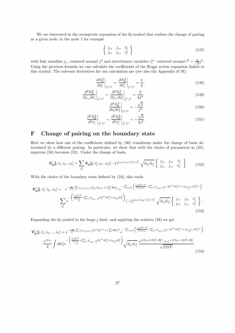
We are interested in the asymptotic expansion of the 6j symbol that realizes the change of pairingat a given node; in the node 1 for example

{

j12 j13 ix

1

j15 j14 iy

1

}

(147)

with link variables j1n centered around j0 and intertwiners variables imn

1 centered around i0 = 2√3j0.

Using the previous formula we can calculate the coefficients of the Regge action expansion linked tothis symbol. The relevant derivatives for our calculation are (see also the Appendix of [9])

∂SAR

∂ix

1

∣

∣

∣

∣

j0,i0=

∂SAR

∂iy

1

∣

∣

∣

∣

j0,i0=

π

2, (148)

∂2SAR

∂j1n∂ix

1

∣

∣

∣

∣

j0,i0=

∂2SAR

∂j1n∂iy

1

∣

∣

∣

∣

j0,i0=

3

4j0, (149)

∂2SAR

∂ix

1∂iy

1

∣

∣

∣

∣

j0,i0= −

√3

j0, (150)

∂2SAR

∂2ix

1

∣

∣

∣

∣

j0,i0=

∂2SAR

∂2iy

1

∣

∣

∣

∣

j0,i0= −

√3

2j0. (151)

F Change of pairing on the boundary state

Here we show how one of the coefficients defined by (36) transforms under the change of basis de-termined by a different pairing. In particular, we show that with the choice of parameters in (24),equation (50) becomes (52). Under the change of basis,

Φ′q[j, ix

1, i2...i5] =∑

iy1

Φq[j, iy

1, i2...i5](−1)j13+j14+ix1+iy

1

√

dix1diy

1

{

j12 j13 ix

1

j15 j14 iy

1.

}

(152)

With the choice of the boundary state defined by (24), this reads

Φ′q[j, ix

1, i2...i5] = e−1

2j0

P

α(ij)(mr)δjijδjmr+iP

Φδjij e−P

n 6=1

„

(δimnn )2

4σimn+P

a φjna i

mnn

δjanδimnn +iχ

imnn

δimnn

«

·∑

iy1

e−

(δiy1 )2

4σiy1

+P

a φja1 i

y1

δja1δiy1+iχ

iy1

δiy1

!

(−1)j13+j14+ix1+iy

1

√

dix1diy

1

{

j12 j13 ix

1

j15 j14 iy

1

}

.

(153)

Expanding the 6j symbol in the large-j limit, and applying the relation (38) we get

Φ′q(j, ix

1, i2, ..., i5) = e− 1

2j0

P

α(ij)(mr)δjijδjmr+iP

Φδjij

e−P

n 6=1

„

(δimnn )2

4σimn+P

a φjna i

mnn

δjanδimnn +iχ

imnn

δimnn

«

· eiπi0

2

∫

dδiy

1e−

(δiy1 )2

4σiy1

+P

a φja1 i

y1

δja1δiy1+iχ

iy1

δiy1

!

√

dix1diy

1

ei(SR+πδiy1+ π

4 ) + e−i(SR−πδiy1+ π

4 )

√12πV

.

(154)

27

We expand the Regge action up to second order in all its 6 entries; the external link around j0 andthe intertwiners around i0

SR[j1n, iy

1, ix

1] =SR[j0, i0] +∂SR

∂j1n

∣

∣

∣

∣

j0,i0δj1n +

∂SR

∂ix

1

∣

∣

∣

∣

j0,i0δix

1 +∂SR

∂iy

1

∣

∣

∣

∣

j0,i0δiy

1 +∂2SR

∂j1n∂j1n′

∣

∣

∣

∣

j0,i0δj1nδj1n′+

+∂2SR

∂j1n∂ix

1

∣

∣

∣

∣

j0,i0δj1nδix

1 +∂2SR

∂j1n∂iy

1

∣

∣

∣

∣

j0,i0δj1nδiy

1 +∂2SR

∂ix

1∂iy

1

∣

∣

∣

∣

j0,i0δix

1δiy

1

+1

2

∂2SR

∂2j1n

∣

∣

∣

∣

j0,i0(δj1n)2 +

1

2

∂2SR

∂2ix

1

∣

∣

∣

∣

j0,i0(δix

1)2 +

1

2

∂2SR

∂2iy

1

∣

∣

∣

∣

j0,i0(δiy

1)2 + ...

(155)

In the background in which we are interested, i0 = 2√3j0 and ∂SR

∂iy1

∣

∣

∣

j0,i0= ∂SR

∂ix1

∣

∣

∣

j0,i0= π

2 . The

value χ = ∂SR

∂iy1

∣

∣

∣

j0,i0= π

2 , yields a phase in the intertwiner variable e−i π2 δiy

1 that cancels one of the

two rapidly-oscillating phase factor due to the linear term of the expansion of the Regge action. In

particular the linear part in the intertwiner variable of the first exponential ei(

∂SR

∂iy1

˛

˛

˛

˛

j0,i0+π)δiy

1

= ei 3π2 δiy

1

combines with the boundary phase factor but the linear part of the second one e−i(

∂SR

∂iy1

˛

˛

˛

˛

j0,i0−π)δiy

1

=ei π

2 δiy1 is canceled: for the same mechanism described in [6] only the second term in the summation

(154) survives. Denoting SR = SR − iπ2 δiy

1, we have that (154) reduces to

Φ′q(j, ix

1, i2, ..., i5) =e− 1

2j0

P

α(ij)(mr)δjijδjmr+iP

Φδjij

e−P

n 6=1

„

(δimnn )2

4σimn+P

a φjna i

mnn

δjanδimnn +i π

2 δimnn

«

·

· eiπi0

2

∫

dδiy

1 e−

(δiy1 )2

4σiy1

+P

a φj1a i

y1

δja1δiy1+i π

2 δiy1

!

√

dix1diy

1

e−i(SR+ π4 )

√12πV

.

(156)

From [9], we have that denoting µ =

√

dix1

diy1

12πV , the dominant term is µ[j0]. We take µ[j0] out ofthe integration and evaluate the integral following [20]. To simplify the notation, rename the second

derivative of the Regge action Gjna,imnn

= ∂2SR

∂jna∂imnn

∣

∣

∣

j0,i0, G

im

n′n ,imn

n= ∂2SR

∂im

n′n ∂imn

n

∣

∣

∣

j0,i0and indicate

with S[jna] (53) the part of the Regge action that depends only on the boundary links involved in the6j symbol considered and with no dependence from the intertwiners. Substituting we get

Φ′q(j, ix

1, i2, ..., i5) =e− 1

2j0

P

α(ij)(mr)δjijδjmr+iP

Φδjij

e−P

n 6=1

„

(δimnn )2

4σimn+P

a φjna i

mnn

δjanδimnn +i π

2 δimnn

«

· eiπi0

2e−i π

4 µ[j0]e−iSR[j0,i0]

· e−iSj [j1a]e−i π2 δix

1 e−i“

P

a Gj1a ix1

δja1”

δix1 e

− i2 Gix

1ix1(δix

1 )2

·∫

dδiy

1 e− 1

2 ( 12σ

iy1

+iGiy1

iy1)(δiy

1 )2

e−iG

ix1 i

y1

δix1δiy

1 e−“

P

a

“

φj1a i

y1+iG

j1a iy1

”

δ ja1”

δiy1

(157)

The choice φ = −iGj1a iy1

= −i 34j0 eliminates the argument of last exponential. So that we fall into

the same as calculation [20], and we can transform the gaussian in another gaussian with the same

28

variance. Evaluating the integral we get

Φ′q(j, ix

1, i2, ..., i5) =e− 1

2j0

P

α(ij)(mr)δjij δjmr+iP

Φδjij

e−P

n 6=1

„

(δimnn )2

4σimn−i“

P

a3

4j0δjan−π

2

”

δimnn

«

·√

π

2( 12σ

iy1

+ iGAiy1 iy

1)· eiπi0e−i π

4 µ[j0]e−iSA[j0,i0]

e−iSAj [j1a]e−i π

2 δix1 e

−i“

P

a Gj1a ix1

δja1”

δix1

e

− 12

0

@

G2ix1

iy1

( 12σ

iy1

+iGA

iy1

iy1

)+iGA

ix1 ix

1

1

A(δix1 )2

(158)

The Gaussian in the last equation has variance

σix1

=1

2

G2ix1 iy

1

( 12σ

iy1

+ iGiy1 iy

1)

+ iGix1 ix

1

−1

(159)

as in [20]. Proceeding in the same way, we fix σ so that both σiy1

and σix1

are real quantities. Remark-

ably the auxiliary tetrahedron described by SR is isosceles and in this case σix1

= σiy1

= j0/3The final form of the coefficient is then

Φ′q(j, ix

1, i2, ..., i5) =e− 1

2j0

P

α(ij)(mr)δjij δjmr+iP

Φδjij

e−P

n 6=1

„

(δimnn )2

4σimn−i“

P

a3

4j0δjan−π

2

”

δimnn

«

·

· N1e−iSj [j1a]e

− 14

1σix

1

(δix1 )2

e−i“

P

a Gj1a ix1

δja1+ π2

”

δix1

(160)

where

N1 =

√

π

2( 12σ

iy1

+ iGiy1 iy

1)eiπi0e−i π

4 µ[j0]e−iSR[j0,i0] (161)

and we have the result (52).Summarizing, the parameters (29) and (30) are determined by the requirement that the gaussian

has the same shape in all bases.

G Simple gaussian integrals used in the calculation

∫ +∞

−∞dxD exp−1

2xaAabx

b =(2π)

D2√

detA, (162)

∫ +∞

−∞dxDxixj exp−1

2xaAabx

b =(2π)

D2√

detAA−1

ij , (163)

∫ +∞

−∞dxD exp−1

2xaAabx

b + iθaxa =(2π)

D2√

detAexp−1

2θaA−1

ab θb, (164)

∫ +∞

−∞dxDxi exp−1

2xaAabx

b + iθaxa =(2π)

D2√

detAi A−1

ia θa exp−1

2θaA−1

ab θb, (165)

∫ +∞

−∞dxDxixj exp−1

2xaAabx

b + iθaxa =(2π)

D2√

detA(A−1

ia θa A−1jb θb − A−1

ij ) exp−1

2θaA−1

ab θb, (166)

∫ +∞

−∞dx xm exp−1

2ax2 + iθx =

√

2π

a(−i)m ∂m

∂θmexp− 1

2aθ2. (167)

29

References

[1] A. Ashtekar, “An introduction to loop quantum gravity through cosmology”, gr-qc/0702030. A.Ashtekar, J. Lewandowski, “Background independent quantum gravity: A status report”, ClassQuant Grav 21 (2004) R53-R152. T. Thiemann, Introduction to Modern Canonical QuantumGeneral Relativity (CUP, to appear).

[2] C. Rovelli, Quantum Gravity, (Cambridge University Press, Cambridge, 2004).

[3] C. Rovelli, L Smolin, “Knot theory and quantum gravity” Phys Rev Lett 61 (1988) 1155-1158. C.Rovelli, L. Smolin, “Loop space representation for quantum general relativity”, Nuclear PhysicsB331 (1990) 80-152. A. Ashtekar, C. Rovelli, L. Smolin, “Weaving a classical geometry withquantum threads”, Phys Rev Lett 69, 237 (1992). C. Rovelli, L. Smolin, “Discreteness of Areaand Volume in Quantum Gravity”, Nucl Phys B442 (1995) 593-619; Nucl Phys B456, 734 (1995).A. Ashtekar, J. Lewandowski, “Quantum Theory of Geometry I: Area Operators” Class QuantumGrav 14 (1997) A55-A82; “II : Volume Operators”, Adv Theo Math Phys 1 (1997) 388-429

[4] L. Modesto, C. Rovelli, “Particle scattering in loop quantum gravity”, Phys. Rev. Lett. 95 (2005),191301, [arXiv: gr-qc/0502036].

[5] C. Rovelli, “Graviton propagator from background–independent quantum gravity” Phys. Rev.Lett. 97 (2006), 151301, [arXiv: gr-qc/0508124].

[6] E. Bianchi, L. Modesto, C. Rovelli, S. Speziale, “Graviton propagator in loop quantum gravity”,Class. Quant. Grav. 23 (2006), 6989-7028; [arXiv: gr-qc/0604044].

[7] S.Speziale “Towards the graviton from spinfoams: the 3d toy model”, JHEP 0605 (2006) 039,[arXiv:gr-qc/0512102].

[8] E. R. Livine, S. Speziale, “Group Integral Techniques for the Spinfoam Graviton Propagator”,JHEP 0611 (2006) 092, [arXiv:gr-qc/0608131].

[9] E. Livine, S. Speziale, J. Willis, “Towards the graviton from spinfoams: higher order correctionsin the 3d toy model”, Phys Rev D 75, 024038 (2007).

[10] B. Dittrich, L. Freidel and S. Speziale, “Linearized dynamics from the 4-simplex Regge action”,arXiv:0707.4513 [gr-qc].

[11] J.W. Barrett and L. Crane, “Relativistic spin networks and quantum gravity”, J. Math. Phys.39, 3296 (1998) [gr-qc/9709028].

[12] JC Baez, JD Christensen, TR Halford, DC Tsang, “Spin Foam Models of Riemannian QuantumGravity”, Class Quant Grav 19 (2002) 4627-4648 [arXiv:gr-qc/0202017v4].

[13] E. Alesci, C. Rovelli, “The complete LQG propagator: II. Asymptotics of the vertex” to appear.

[14] R. De Pietri, L. Freidel, K. Krasnov and C. Rovelli, “Barrett-Crane model from a Boulatov-Oogurifield theory over a homogeneous space,” Nucl. Phys. B 574, 785 (2000) [arXiv:hep-th/9907154].D Oriti, RM Williams, “Gluing 4-simplices: a derivation of the Barrett-Crane spinfoam modelfor Euclidean quantum gravity”, Phys Rev D63(2001) 024022. A. Perez and C. Rovelli, “FiniteSO(4)-state sum model of Euclidean GR,” Prepared for 9th Marcel Grossmann Meeting on RecentDevelopments in Theoretical and Experimental General Relativity, Gravitation and RelativisticField Theories (MG 9), Rome, Italy, 2-9 Jul 2000 A. Perez and C. Rovelli, “A spin foam modelwithout bubble divergences,” Nucl. Phys. B 599, 255 (2001) [arXiv:gr-qc/0006107].

30

[15] M. P. Reisenberger, “A lattice worldsheet sum for 4-d Euclidean general relativity,”[arXiv:gr-qc/9711052].

[16] J. Engle, R. Pereira, C. Rovelli “The loop-quantum-gravity vertex-amplitude”, [arXiv:0705.2388].

[17] E. R. Livine and S. Speziale, “A new spinfoam vertex for quantum gravity,” [arXiv:0705.0674,gr-qc].

[18] S. Alexandrov, “Spin foam model from canonical quantization”, arXiv:0705.3892 [gr-qc].

[19] C. Rovelli, L. Smolin “Spin Networks and Quantum Gravity”, Phys.Rev. D 52 (1995) 5743-5759,[arXiv:gr-qc/9505006].

[20] S. Speziale, C. Rovelli, “A semiclassical tetrahedron”, Class.Quant.Grav. 23 (2006) 5861-5870[arXiv: gr-qc/0606074].

[21] G.Ponzano and T.Regge, “Semiclassical limit of Racah coefficients” in Spectroscopic and grouptheoretical methods in physics (Bloch ed.), North-Holland, 1968.

[22] L. Freidel and D. Louapre, “Asymptotics of 6j and 10j symbols,” Class. Quant. Grav. 20, 1267(2003) [arXiv:hep-th/0209134].

[23] J. W. Barrett and R. M. Williams, “The asymptotics of an amplitude for the 4-simplex,”Adv. Theor. Math. Phys. 3 (1999) 209 [arXiv:gr-qc/9809032]. J. C. Baez, J. D. Chris-tensen and G. Egan, “Asymptotics of 10j symbols,” Class. Quant. Grav. 19 (2002) 6489[arXiv:gr-qc/0208010]. J. W. Barrett and C. M. Steele, “Asymptotics of relativistic spin net-works,” Class. Quant. Grav. 20 (2003) 1341 [arXiv:gr-qc/0209023]. J. D. Christensen andG. Egan, “An efficient algorithm for the Riemannian 10j symbols,” Class. Quant. Grav. 19

(2002) 1185 [arXiv:gr-qc/0110045].

[24] D. Oriti, “The group field theory approach to quantum gravity,” [arXiv:gr-qc/0607032]. L Freidel,“Group Field Theory: an overview”, Int. J. Theor. Phys. 44 (2005) 1769-1783.

[25] D. M. Brink, G. R. Satchler, Angular Momentum (Claredon Press, Oxford, 1968).

[26] R. De Pietri, C. Rovelli “Geometry Eigenvalues and Scalar Product from recoupling Theory inLoop Quantum Gravity”, Phys. Rev. D 54 (1996) 2664-2690 , [arXiv:gr-qc/9602023].

[27] R. De Pietri “On the relation between the connection and the loop representation of quantumgravity”, Class. Quant. Grav. 14 (1997) 53-70, [arXiv:gr-qc/9605064].

31