Linking covariant and canonical LQG: new solutions to the Euclidean Scalar

Constraint

Emanuele Alesci,∗ Thomas Thiemann,† and Antonia Zipfel‡

Universitat Erlangen, Institut fur Theoretische Physik III,

Lehrstuhl fur Quantengravitation

Staudtstrasse 7, D-91058 Erlangen, EU

Abstract It is often emphasized that spin-foam models could realize a projection on the physical Hilbert

space of canonical Loop Quantum Gravity (LQG). As a first test we analyze the one-vertex expansion of a

simple Euclidean spin-foam. We find that for fixed Barbero-Immirzi parameter γ = 1 the one

vertex-amplitude in the KKL [14] prescription annihilates the Euclidean Hamiltonian constraint of LQG

[5]. Since for γ = 1 the Lorentzian part of the Hamiltonian constraint does not contribute this gives rise to

new solutions of the Euclidean theory. Furthermore, we find that the new states only depend on the

diagonal matrix elements of the volume. This seems to be a generic property when applying the spin-foam

projector.

∗ alesci@theorie3.physik.uni-erlangen.de† thiemann@theorie3.physik.uni-erlangen.de‡ zipfel@theorie3.physik.uni-erlangen.de

arX

iv:1

109.

1290

v1 [

gr-q

c] 6

Sep

201

1

1

CONTENTS

I. Introduction 1

A. Motivation 1

B. Outline 4

II. Hamiltonian constraint 4

A. Hamiltonian constraint 5

B. Properties 7

C. Action on a trivalent node 8

D. Action on a 4-valent node 10

III. Spin-foam 11

A. The model 11

B. Spin-foam projector 13

IV. New solutions to the Euclidean Hamiltonian constraint 14

A. Trivalent nodes 15

B. Four valent nodes 19

V. Conclusions 21

A. Graphical Calculus 22

1. Basic Elements 22

2. Recoupling and Simplifications of graphs 24

B. Grasping 27

C. Normalization of the spin-network states 28

References 29

I. INTRODUCTION

A. Motivation

One mayor problem when quantizing Gravity is the constrained algebra, which completely deter-

mines the theory, and background independence. Canonical Loop Quantum Gravity [1–3] follows

the ideas of Dirac [4] for quantizing constrained systems and preserves background independence.

The kinematical Hilbert space Hkin of LQG is spanned by spin-network functions living on semi-

analytic closed graphs embedded in a three dimensional spatial hyper-surface Σ of a 4-dimensional

2

manifold M. Diffeomorphism and gauge constraints can be embedded via a group averaging pro-

cedure. The remaining constraint (Hamiltonian) is more complicated. Even though a quantization

of the latter has been found [5, 6], the structure of the physical Hilbert space Hphys is not fully

understood up till now.

To circumvent the problems of the canonical theory Reisenberger and Rovelli [7] introduced a

covariant formulation of Quantum Gravity, the so-called spin-foam model [8, 9]. This model is

mainly based on the observation that the Holst action for GR [10] defines a constrained BF-theory.

The strategy is first to quantize discrete BF-theory and then to implement the so called simplic-

ity constraints. The main building block of the model is a linear two-complex κ embedded into

4-dimensional space-time M whose boundary is given by an initial and final (gauge invariant)

spin-network, ψi respectively ψf , living on the initial respectively final spatial hyper surface of a

foliation of M. The physical information is encoded in the spin-foam amplitude

Z[κ] =∏f

Af∏e

Ae∏v

Av × B (I.1)

where Af ,Ae and Av are the amplitudes associated to the internal faces, edges and vertices1

of κ and B contains the boundary amplitudes. Each spin-foam can be thought of as generalized

Feynman diagram contributing to the transition amplitude from an ingoing spin-network to an

outgoing spin-network. By summing over all possible two-complexes one obtains the complete

”transition amplitude” between ψi and ψf .

Unfortunately the simplicity constraint is second-class and the procedure how to implement it is

still under debate [11]. Nevertheless substantial progress has been achieved during the last years

[12]. Especially, the introduction of a new vertex amplitude by Engle, Pereira, Rovelli and Livine

and independently by Freidel and Krasnov [13] and the introduction of an abstract model [14] led

to a major breakthrough.

Instead of considering spin-foams as a ”sum over histories” one could equally well think of spin-

foams as some group averaging procedure to implement the Hamiltonian constraint in the canonical

formalism (see [7, 15]). Suppose we have a family of first-class constraints (CI)I∈I which form a Lie-

algebra. Generically, the point zero does not lie in the point spectrum of the constraint operators

and therefore the eigenvectors can not form the entire solution space. To obviate this problem one

has to consider generalized eigenvectors l ∈ D∗kin in the algebraic dual of a dense domain of Hkin

such that [(CI)

′l]

(ψ) := l(C†Iψ) = 0 ∀ I ∈ I, ψ ∈ Dkin (I.2)

where (CI)′ is the dual operator on D∗kin. The space of generalized solutions D∗phys is a proper

subspace of D∗kin. In order to construct a physical Hilbert space one considers D∗phys as the algebraic

1 In the following we will call edges and vertices in the boundary links respectively nodes to distinguish between the

two-complex and the graph.

3

dual of a dense subspace Dphys ⊂ Hphys so that all observables are densely defined in Hphys. The

inner product onHphys is chosen such that adjoints in the physical scalar product represent adjoints

in the kinematical one. It can be systematically constructed by an anti-linear map, called rigging

map,

η : Dkin → D∗kin (I.3)

such that

〈η[φ]|η[ψ]〉phys := η[φ](ψ) φ, ψ ∈ Dkin (I.4)

and

O′η[φ] = η[Oφ] ∀φ ∈ Dkin . (I.5)

The physical Hilbert space is subsequently defined by the completion of Dphys := η(Dkin) \ker(η).2

Strictly speaking, such a construction only works for closed, first-class constraints. But the con-

straint algebra in GR is open with structure functions instead of structure constants. Nevertheless,

it is often emphasized that spin-foams could provide such a rigging map even though one starts

with a different action and constraint algebra than in the canonical approach. If this is indeed the

case then the physical inner product would be given by

〈φ|ψ〉phys =∑κ:ψ→φ

Z[κ] (I.6)

and the rigging map would correspond (schematically) to

η[ψ] =∑

φ∈Hkin

∑κ:ψ→φ

Z[κ]〈φ| . (I.7)

Since all constraints are satisfied in Hphys the so-defined physical scalar product must obey

〈ψout|C†|ψin〉phys =∑

φ∈Hkin

∑κ:ψout→φ

Z[κ]〈φ|C†|ψin〉kin = 0 (I.8)

for all ψout, ψin ∈ Hkin. This is clearly the case for the gauss constraint because the boundary

of a spin-foam are gauge invariant spin-networks. The diffeomorphism constraint is harder to

deal with since spin-foams are defined on a discretization of space-time and break diffeomorphism

invariance. But in the abstract formulation the amplitudes do not depend on the embedding and

one can implement the constraint by restricting on equivalence classes of spin-networks. Wether the

Hamiltonian constraint also obeys (I.8) depends crucially on the definition of the vertex amplitudes.

However, it is fcrucially to solidify LQG results that compute transition amplitudes assuming the

EPRL-FK model as defining the dynamics of the theory in the context of the propagator [33, 36, 37]

2 For more details on the construction of a rigging map see e.g. [2].

4

B. Outline

As a first test for (I.8) we consider an easy spin-foam amplitude and show that∑φ

Z[κ]〈φ|Hn|ψin〉 = 0 (I.9)

where κ is a two-complex with only one internal vertex such that φ is a spin-network induced on

the boundary of κ and Hn is the Hamiltonian constraint acting on the node n.

In Sec. II. we briefly review the quantization of the Hamiltonian constraint [5] and compute

the action on three- and four-valent nodes by employing graphical calculus. Recall, that the full

constraint C = −[H + (s− γ2)HL] can be decomposed into its Lorentzian and Euclidean part, HL

respectively H where γ is the Barbero-Immirzi parameter and s is the signature of the metric. We

restrict the analysis to the Euclidean sector with s = 1, γ = 1. Then C reduces to the Euclidean

part only. The operator H acts locally on nodes and is graph-changing. We choose a tetrahedral

regularization of the latter as proposed in [5]. Then roughly speaking, H creates a new link

connecting two pairwise distinct links adjacent to the same node. In order to keep the calculation

as simple as possible we choose ψout = ψin being a spin-network with two n-valent nodes.

We will summarize the construction of the spin-foam amplitude in Sec.III.

In the subsequent section we evaluate the spin-foam amplitude for a two-complex κ with only one

internal vertex and boundary ∂κ = ψout ∪ φ such that κ is a tube ψout × [0, 1] with an additional

face between the internal vertex and the new link created by H (see Fig.2).

In Sec. IV we show that the one-vertex amplitude annihilates the Hamiltonian constraint by

employing basic summation identities of 6j-symbols, when acting on three respectively four-valent

nodes. For an n-valent node the sum (I.9) is a sum over spin-networks based on(n2

)different

graphs. Remarkably, each partial sum over spin-networks based on the same graph vanishes. This

shows, that the solutions constructed via the spin-foam method build a proper subset of Hphys. As

an important side result we find that∑

φ Z[κ]〈φ| selects only those matrix elements of H which

depend on the diagonal matrix elements of the volume.

Sec. V contains a summary of our results and give an outlook to open questions.

II. HAMILTONIAN CONSTRAINT

A primary quantum version of the Hamiltonian constraint operator was introduced by Rovelli

and Smolin [16]. The operator proofed to act only on the nodes of a spin-network function. But

it was divergent on general states. Latter [17], it was shown that the following two properties are

crucial in order to obtain a well defined finite Hamiltonian operator in the background independent

context:

• the operator needs to be a density (more precisely, a three-form)

5

• diffeomorphism invariance trivializes the limit when the regulator is removed from the oper-

ator.

The first requirement forces us to use a non-polynomial version of the constraint which quantization

is much more involved. After many efforts [18–20], it was suggested [5, 6] to express the inverse triad

e as the Poisson bracket between the volume V and the holonomy h of the Ashtekar connection A:

e ∼ h−1[h, V ]. This trick made it possible to construct an Hamiltonian with the above properties

which can be regularized on a given triangulation T of the space manifold. (For criticism see [21].)

In the following two sections we will review the basic construction of C as proposed in [5] in order

to clarify the model and our notation. The reader familiar to the framework can easily skip the

next two sections.

A. Hamiltonian constraint

The classical Hamiltonian constraint is

C = −2

κTr[( (γ)F − (γ2 − s)K ∧K) ∧ e] (II.1)

where e = eiaτidxa is the inverse triad, K the extrinsic curvature, (γ)F the curvature of the Ashtekar

connection with real Immirzi parameter γ and s the signature. In the following we choose units

such that κ/2 := 8πGc3

= 1.

The constraint can be split into its “Euclidean” partH = Tr[F∧e] and Lorentzian partHL = C−H.

Following [5], we can rewrite (II.1) by using

eia = −2{Aia(x), V }Kia = 2{Aia(x),K}K = 2{H,V }

(II.2)

where V is the volume of an arbitrary region Σ containing the point x. Smearing the constraints

with lapse function N(x) gives

H[N ] =

∫Σd3xN(x)H(x)

=− 2

∫ΣN Tr(F ∧ {A, V })

(II.3)

HL[N ] =

∫Σd3xN(x)HL(x)

= −(γ2 − s)∫

ΣN Tr({A, {HL, V }} ∧ {A, {HL, V }} ∧ {A, V }) .

(II.4)

This expression requires a regularization in order to obtain a well-defined operator on Hkin. Up to

now there exist many different proposals (see e.g [1, 22]). We will follow the original proposal [5]

and use a triangulation T of the manifold Σ into elementary tetrahedra with analytic links adapted

6

aki

n si

sjsk aij

ajk

Figure 1. An elementary tetrahedron ∆ ∈ T constructed

by adapting it to a graph Γ which underlies a cylindrical

function.

to the graph Γ of an arbitrary spin-network. For each pair of links ei and ej incident at a node

n of Γ we choose semi-analytic arcs aij such that the end points sei , sej are interior points of ei

respectively ej and aij ∩ Γ = {sei , sej}. The arc si is the segment of ei from n to si and si, sj and

aij generate a triangle αij := si ◦ aij ◦ s−1j . Three (non-planar) links define a tetrahedron (see Fig.

1). Now we can decompose (II.3) into a sum of one term per each tetrahedron of the triangulation

H[N ] =∑∆∈T−2

∫∆d3xN εabc Tr(Fab{Ac, V }) . (II.5)

Define the classical regularized Hamiltonian constraint

HT [N ] :=∑∆∈T

H∆[N ] . (II.6)

The connection A respectively the curvature are regularized as usual by the holonomy hs := h[s] ∈SU (2) (in the fundamental representation m = 1/2) along the segments si respectively along the

loop αij . This yields

H∆[N ] : = −2

3N(n) εijk Tr

[hαijhsk

{h−1sk, V}]

(II.7)

and converges to the Hamiltonian constraint (II.5) if the triangulation is sufficiently fine. The

expression (II.6) can finally be promoted to a quantum operator, since volume and holonomy have

corresponding well-defined operators in LQG. The lattice spacing of the triangulation T that acts

as a regularization parameter can be removed in a suitable operator topology, see [5] for details.

Remarks

• In [28] it was pointed out that the operator can be immediately generalized by replacing

the trace in (II.5) with a trace in an arbitrary irreducible representation m: Trm[U ] =

Tr[R(m)(U)] where R(m) is a matrix representation of U ∈ SU (2). Equation (II.7) can thus

be replaced by

Hm∆ [N ] :=

N(n)

N2m

εijk Tr[h(m)αij

h(m)sk

{h(m)−1sk

, V}]

, (II.8)

7

N2m = Trm[τ iτ i] = −(2m+1)m(m+1) and h(m) = R(m)(h). As shown in [28], this converges

to H[N ] as well.

• The Lorentzian part of the constraint can be regularized by a similar method.

B. Properties

In this section we will summarize the important properties of the Euclidean Hamiltonian con-

straint.

It is immediate to see that when acting on a spin-network state, the operator reduces to a sum

over terms each acting on individual nodes. Acting on nodes of valence n the operator gives

HmΓ [N ]ψΓ =

i

~∑

n∈N (Γ)

∑n(∆)=n

p∆

E(n)Hm

∆ [N ]ψΓ , (II.9)

where Hm∆ is the quantum version of (II.8), N (Γ) is the set of nodes of Γ and E(n) =

(n3

)is

the number of unordered triples of links adjacent to n. The second sum is a sum over tetrahedra

with a node at n and not intersecting with other nodes of Γ. Moreover, p∆ = 1, whenever ∆ is a

tetrahedron having three edges coinciding with three links of the spin-network state, that meet at

the node n, otherwise p∆ = 0.

On diffeomorphism invariant states φ ∈ Hphys ⊂ H∗kin the regulator dependence drops out trivially

because two operators H and H ′ that are related by a refinement of the triangulation differ only

in the size of the loops αij . Therefore, the resulting states are in the same equivalence class and

[H†φ](ψ) := 〈φ, Hψ〉 = 〈φ, H ′ψ〉 , (II.10)

in Hdiff . This proves that the Hamiltonian constraint on diffeomorphism invariant states is inde-

pendent from the refinement of the triangulation.

The action H(N) on a spin-network state TΓ,~j,~c defined on a graph Γ results in a finite linear com-

bination of spin-network states defined on graphs ΓI where Γ ⊂ ΓI and aI := ΓI − Γ is produced

by one of the arcs aij(∆), which carries spin jI = m. The new nodes are called extra ordinary. In

some cases it can happen that links connecting the original node with the new extraordinary nodes

carry trivial representation if this is allowed by the recoupling conditions. Extraordinary nodes

are at most trivalent and intersections of precisely two analytic curves c, c′ ⊂ Γ, that is, n = c∩ c′,such that n is an endpoint of c but not of c′. A link e of a graph Γ is called extraordinary provided

that its endpoints n1, n2 are both extraordinary nodes. Furthermore, those links are adversed to a

node n of γ which is incident to at least three links s1, s2, s3 with linearly independent tangents at

n such that s1/s2 connect n and n1/n2. We will call n the typical node associated with e. All links

produced by H are extraordinary. Since the volume operator annihilates coplanar nodes and gauge

invariant nodes of valence three (only true for Ashtekar-Lewandowski version, see [1]) H does not

act on extraordinary nodes.

8

C. Action on a trivalent node

Let us now compute the action of the operator Hm∆ on a trivalent node where all links are

outgoing, following [22, 28]. Denote a trivalent node by |n(ji, jj , jk)〉 ≡ |n3〉, whereas ji, jj , jk are

the spins of the adjacent links ei, ej , ek:

|n3〉 =+

jk

ji jj

(II.11)

Note, the links are also labeled by group elements with orientations indicated by the arrows. In

order to simplify the graphics we only displayed the node and its adjacencies. Furthermore, every-

thing contained in the dashed circle belongs to the node and everything between the dashed lines

belong to the same link.

When quantizing expression (II.8) the holonomies and the volume are replaced by their correspond-

ing operators and the Poisson bracket is replaced by a commutator. Since the volume operator

vanishes on a gauge invariant trivalent node we only need to compute

Hm∆ |n3〉 = Nn ε

ijk Tr

(h(m)[αij ]− h(m)[αji]

2h(m)[sk] V h

(m)[s−1k ]

)|n3〉 , (II.12)

where all (global) constants have been absorbed in the lapse function Nn. Antonia The operator

h(m)[s−1k ], corresponding to the holonomy along a segment sk with reversed orientation, acts by

multiplication with R(m)(hs−1k

) along sk. The matrix R(m) can be recoupled using (A.12) and

(A.10). Thus, h(m)[s−1k ] creates a free index in the m-representation located at the node (inside

the dashed circle), making it non-gauge invariant and a new node on the link ek:

h(m)[s−1k ] |n3〉 = (−1)2m

∑c

dc+

jk

jk+

−c

m

m

ji jj

(II.13)

9

where dc = 2c+ 1 is the dimension of c. The range of the sum over the spin c is determined by the

Clebsch-Gordan conditions and the little flag represents the group element h−1sk

.

The volume operator now acts on a trivalent non-gauge invariant node with a virtual link in jk

representation. The matrix elements of the volume operator [23–25], have been computed in [26, 27]

and the results have been applied to the Hamiltonian constraint operator in [28, 29].

The operators h(m)[αij ]h(m)[sk] and h(m)[αji]h

(m)[sk] add open loops with opposite orientations

αij and αji, where we fix αij to be oriented anti-clockwise. Like above, the representations living

on the same link can be recoupled. The m-trace connects the free ends of the open loops to the

two open links in h(m)[s−1k ] |n〉 taking into account the orientations. Finally one has to use (A.17):

Tr

(h(m)[αij ]− h(m)[αji]

2h(m)[sk]V h

(m)[s−1k ]

)|n(ji, jj , jk)〉

=∑a,b

A(m)(ji, a|jj , b|jk)+

jk

ji

+

jj

+

a b

m

(II.14)

where the range of the sums over a, b is determined by the Clebsch-Gordan conditions3 and

A(m)(ji, a|jj , b|jk) :=∑c

λmjia λmjjb λmjkc (−)ji+jj−jk dadbdc

×∑

β(ji,jj ,m,c)

V jkβ(ji, jj ,m, c) (II.15)

×[λmβc (−)a+jj+c { a jj c

β m ji}{ a b jk

m c jj} − λmjkc (−)b+ji+c{ ji b c

m β jj}{ a b jk

c m ji}].

The sign factors are due to the chosen orientation which has to be respected when applying the

recoupling identities (see A) and can be manipulated by realizing that (−)2a+2b+2c = 1 if a, b, c

fulfill the Clebsch-Gordan conditions. The summation index β = β(ji, jj ,m, c) which appears due

to the non-diagonal action of the volume operator, ranges on the values which are determined by

the simultaneous admissibility of the trivalent nodes {ji, jj , β} and {m, c, β}. If m = 12 then the

volume operator acts diagonally and β = jk.4

The complete action of the operator on a trivalent state |n(ji, jj , jk)〉 can be obtained by contracting

the trace part (II.14) with εijk. Thus, H projects on a linear combination of three spin-networks

which differ by exactly one new link labeled by m between each couple of the ’old’ links at the

node.

3 The link m can not be removed with (A.17) since this is a pure recoupling identity but m also carries a group

element.4 We get a correction of sign factors compared to [22]. This correction is necessary in order that the action of Tr(Fij)

vanishes.

10

D. Action on a 4-valent node

The computation for a 4-valent node |n4〉 is similar to the previous:

Hm∆ |n4〉 = Nn ε

ijk Tr

(h(m)[αij ]− h(m)[αji]

2h(m)[sk] [V , h(m)

[s−1k ]])|n4〉 . (II.16)

In the subsequent calculation we fix choose all links to be outgoing from the node

|n4〉 =√di +

jl

ji

+

jk

jj

i(II.17)

where i labels the intertwiner (inner link). Furthermore, we fix the orientation of the loop αij

in (II.16) to be anti-clockwise. The part Tr(h(m)[αij ]− h(m)[αji] V

)|n4〉 vanishes since the vol-

ume does not modify the representations but the trace is taken in the representation space and

Tr(h(m)[αij ]− h(m)[αji]) = 0.

For the other part, the holonomy h(m)[s−1k ] changes the valency of the node and the Volume sub-

sequently acts on the 5-valent non-gauge invariant node. Graphically this corresponds to

V h(m)[s−1k ] |n4〉 = (−1)2m

∑c

dc∑β,γ

V γ,βi,jk

+

jl

ji

+

jk

jj

i. (II.18)

Finally one arrives at

Tr

(h(m)[αij ]− h(m)[αji]

2h(m)[sk] V h

(m)[s−1k ]

)|n4〉 =

∑a,b,c

dadbdc∑β,γ

V γ,βi,jk

[+

γ

jl

+

−

+

−−

c

−−

ji

a

ji

β

jk

jj

b

jjm

m

m− +

γ

jl

+

−

+

+

+c

−−

ji

a

ji

β

jk

jj

b

jjm

m

m ] (II.19)

11

This can be simplified using (B.2) and (A.17)

Hm∆ |n4〉 =

∑a,b,c

dadbdc∑β,γ

V γ,βi,jk

[(−1)2ji+a+jl−jj−β+m

∑α

dα

{γ α m

a ji jl

}{γ α m

c β jj

}+

α

jl

−

+

−

−−

a

ji

c

jk

jj

b

jjm

m

− (−1)γ+jj+c+m

{γ jj β

m c b

}+

γ

jl

+

−

+

+

−

ji

a

ji

c

jk

b

jjm

m ]

=∑a,b,c

dadbdc∑β,γ

V γ,βi,jk

(−1)2ji+jl+jj+a+m∑α

dα

[(−1)α+β−c−jj{ γ α m

a ji jl }{γ α mc β jj }{

α jj cm jk b

}

− (−1)c+γ−b−jk{ γ jj βm c b

}{ γ α ma ji jl }{

γ α mjk c b }

]+

jl

−ji

+

jk

−jj

α

a b

m

(II.20)

The sign factors are due to the chosen orientation and can be manipulated as above.

III. SPIN-FOAM

A. The model

In this section we briefly recall the definition of Euclidean spin-foam models as suggested by

Kaminski, Kisielowski and Lewandowski [14] and clarify our notation. Since we are only interested

in the evaluation of a spin-foam amplitude we choose a combinatorial definition of the model.

Consider an oriented two-complex κ defined as the union of the set of faces (2-cells) F , edges (1-

cells) E and vertices (0-cells) V such that every edge e is a 1-face5 of at least one face f (notation:

e ∈ ∂f) and every vertex vis a 0-face of at least one edge e (notation: v ∈ ∂e). We call edges which

5 For a definition of complex see e.g. [30]

12

are contained in more than one face f internal and denote the set of all internal edges by Eint. Vice

versa all vertices adjacent to more than one internal edge are also called internal and denote the

set of these vertices by Vint. The boundary ∂κ is the union of all external vertices (called: nodes)

n /∈ Vint and external edges (called: links) l /∈ Eint. If ∂κ forms a closed but possibly disconnected

graph and the orientation of e ∈ ∂κ agrees with the orientation induced by the unique face f, e ∈ ∂f(we say: f is ingoing to e) then κ is called a proper foam. In the following we will only consider

proper foams.

A spin-foam is a triple (κ, ρf , Ie) consisting of a proper foam whose faces are labeled by irreducible

representations of a Lie-group G (here SO (4)) and whose internal edges are labeled by intertwiners

I. This induces a spin-network structure ∂(κ, ρlf , Ine) on the boundary of κ. In the following we

will denote the pair (v, f) such that v ∈ ∂f by vf and analogously for all other pairings ev, ef etc.

Furthermore ∂v is the set of all faces fv and edges ev.

Suppose κ is foam without boundary. Following [31], we label each edge e ∈ κ by an group element

e→ Ue ∈ SO (4) such that

Ue = ges(e)g−1et(e)

(III.1)

where s(e) / t(e) is the source / target of e. For each pair (v, f) with v∩f = v and edges e∩e′ = v,

e, e′ ∈ ∂f we define

gfv := (g−1ev ge′v)εef (III.2)

where εef = ± according to the orientations. With this definitions the BF partition function can

be rewritten as

ZBF [κ] =

∫SO(4)

dgfv∏f∈κ

δ

∏v∈∂f

gfv

∏fv

∫dgevδ(g

−1fvgevg

−1e′v )︸ ︷︷ ︸

Av(gfv )

(III.3)

Note, Av(gfv) defines an SO (4) invariant function on the graph Γv induced on the boundary of

the vertex v [31]. As it is well known, the boundary Hilbert space Hv is spanned by (normalized)

spin-network functions TBFΓv ,ρ,I(gf )6

Av(gf ) =∑ρf ,Ie

∏f∈∂v

√dim ρf Trv

(⊗e∈∂v

I†e

)TBFΓv ,ρ,I(gf ) (III.4)

Locally SO (4) ∼ SU (2) × SU (2) which implies ρSO(4) = ρ+SU(2) ⊗ ρ−SU(2) and TBFΓv ,ρ,I

(gf ) =

TΓv ,j+,ι+(g+f )⊗ TΓv ,j−,ι−(g−f ).

In the EPRL model [13] the simplicity constraint is imposed weakly. Consequentially, we have to

6 The links lf bounding the face f are labeled by irreducible representations ρf and nodes ne bounding the edge e

are labeled by intertwiners Ie as usual.

13

restrict Av(gf ) to the EPRL subspace HEPRLv spanned by the functions

TEΓv ,jf ,ιe=∏fv

√dj+fv

dj−fv

∏ev

ιAe1···AeFe

∏f∈∂v

Cm+

efm−ef

Aef

∏

(e,f)∈∂v

[εn+efn+

e′f ε

n−ef n−e′f R

j+f

m+efn+ef

(g+ef

) Rj+f

m−ef n−ef

(g−ef )

] (III.5)

with j± ≡ |γ±1|2 j. Furthermore, Rj(g) denotes a Wigner matrix, C

m+e m−E

Aea Clebsch-Gordan coeffi-

cient and εn+e n−e represent the unique two-valent intertwiners of SU (2) (see [31]).

It follows immediately that

AEv (gf ) =∑jf ,ιe

〈TEΓv ,jf ,ιe|Av〉 TEΓv ,jf ,ιe

(gf )

:=∑jf ,ιe

∏f∈∂v

√dj+f

dj−f

AEv (jf , ιe) TEΓv ,jf ,ιe

(gf )

(III.6)

defines the EPRL vertex amplitude with

AEv (jf , ιe) =∑ι+e ,ι−e

Trv

(⊗ev

(ι+ev ⊗ ι−ev)†)∏

ev

fιevι+ev ,ι

−ev

(III.7)

where f ιeι+e ,ι−e

are the well known fusion coefficients [13]. At last one has to replace (III.6) in (III.3)

to obtain the full transition amplitude of the EPRL model. Expanding the delta function in (III.3)

in terms of spin-network function and integrating over the group elements gives

Z[κ] =∑jf ,ιe

∏f

dj+fdj−f

∏v

AEv (jf , ιe) . (III.8)

Remark

In order to evaluate the fusion coefficients f ιeι+e ,ι−e

by graphical calculus it is convenient to work with

3j-symbols instead of Clebsch-Gordan coefficients. When replacing the Clebsch-Gordan coefficients

we have to multiply by an overall factor∏e

∏fe

√2jfe + 1.

B. Spin-foam projector

Instead of using spin-foams as a tool to compute ’transition’ amplitudes between spin-networks

one is tempted to interpret spin-foams as a projector onto the physical Hilbert space. Given any

couple of ingoing and outgoing kinematical states ψout, ψin, the Physical scalar product can be

formally defined by

〈ψout|ψin〉phys := [η(ψout)](ψin) (III.9)

14

where η is a projector (Rigging map) onto the Kernel of the Hamiltonian constraint. Suppose that

the transition amplitude Z

〈ψout|Z|ψin〉 := [η(ψout)](ψin) (III.10)

can be expressed in terms of a sum of spin-foams (κ, ρ, ι) with boundary ∂(κ, ρ, ι) = ψout⋃ψin.

To realize that, we first have to reconsider (III.3) for a foam κ with non-empty boundary ∂κ 6= ∅.Then7

Z[κ] =

∫SO(4)Vint

dgfv∏f∈κ

δ

∏v∈∂f

gfvgl

∏v∈Vint

Av(gfv) (III.11)

where

gl =

hl if f ∩ ∂κ = l

1 otherwise. (III.12)

Equation (III.11) can be interpreted as a function on the boundary graph ∂κ. That is to say

Z[κ] =∑jf ,ιe

∏f

dj+fdj−f

∏v∈Vint

AEv (jf , ιe)

×∑jl,ιn

∏l∈∂κ(1)

1√dj+l

dj−l

TE∂κ,jl,ιn(hl)

(III.13)

in the EPRL sector. Here, ∂κ(1) is the set of boundary links. Unfortunately, (III.13) defines an

SO (4) spin-network function while the kinematical Hilbert space of the canonical theory is spanned

by SU (2) functions. It is, however, easy to resolve that problem: when restricting the boundary

elements hl ∈ SU (2) ⊂ SO (4) then TE∂κ,jl,ιn(hl) is a true SU (2) spin-network function. Indeed

TE∂κ,jl,ιn(hl) =

∏l∈∂κ

√dj+l

dj−ldjl

|S(∂κ, j, ι〉)N (III.14)

where |S〉N is a normalized spin-network function on SU (2) (see C). This finally implies

〈ψout|Z|ψin〉 =∑jf ,ιe

∏f

dj+fdj−f

∏l∈∂κ(1)

1√djl

∏v∈Vint

AEv (jf , ιe) . (III.15)

In the next section we will compute an easy example of such an amplitude.

IV. NEW SOLUTIONS TO THE EUCLIDEAN HAMILTONIAN CONSTRAINT

In the following we compute new solutions to the Euclidean Hamiltonian constraint by employing

spin-foam methods. We show that∑φ

〈ψout|Z[κ]|φ〉〈φ|H(m)|ψin〉 = 0 . (IV.1)

7 If we would also integrate over group elements in the boundary then ZBF =∫δ(F ) would become singular.

15

v

m

ji

jk

jj

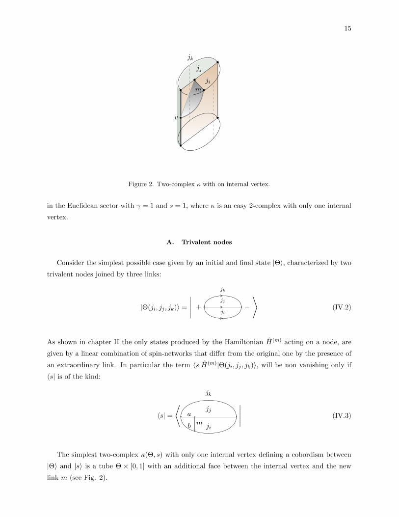
Figure 2. Two-complex κ with on internal vertex.

in the Euclidean sector with γ = 1 and s = 1, where κ is an easy 2-complex with only one internal

vertex.

A. Trivalent nodes

Consider the simplest possible case given by an initial and final state |Θ〉, characterized by two

trivalent nodes joined by three links:

|Θ(ji, jj , jk)〉 =

∣∣∣∣∣ + −

jk

jj

ji

⟩(IV.2)

As shown in chapter II the only states produced by the Hamiltonian H(m) acting on a node, are

given by a linear combination of spin-networks that differ from the original one by the presence of

an extraordinary link. In particular the term 〈s|H(m)|Θ(ji, jj , jk)〉, will be non vanishing only if

〈s| is of the kind:

〈s| =⟨

ji

jk

jja

b m

∣∣∣∣∣ (IV.3)

The simplest two-complex κ(Θ, s) with only one internal vertex defining a cobordism between

|Θ〉 and |s〉 is a tube Θ × [0, 1] with an additional face between the internal vertex and the new

link m (see Fig. 2).

16

The computation of (III.13) for κ(Θ, s) is straightforward when using graphical calculus. Since

the space of three-valent intertwiners is one-dimensional and all labelings jf are fixed by the states

|s〉, |Θ〉 the first sum in (III.13) is trivial. Thus

〈Θ|Z[κ]|s〉 := WE(κ,Θ, s) = Af B AEv (jf , ιe) (IV.4)

where Af =∏f dj+f

dj−fare the face amplitudes and B =

∏l∈∂κ(1)

1√djl

are the boundary ampli-

tudes. The evaluation of the trace in AEv is equivalent to evaluating the boundary spin-network

Γv of the vertex v [31] at 1. The reader can easily convince herself that Γv = s and therefore with

(A.17) gives

Trv(⊗e

ι+e ι−e ) = (−)j

+i +j+j −j

+k (−)j

−i +j−j −j

−k

{j+i j+

j j+k

b+ a+ m+

}{j−i j−j j−kb− a− m−

}. (IV.5)

where the sign factor is due to the orientation of s (see (II.14)).The fusion coefficients contribute

four 9j symbols since

f ιeι+e ,ι−e

=√dadbdc

[ a

c

a+

a−

b

c+ c−

b−

b+

]=√dadbdc

a b c

a+ b+ c+

a− b− c−

(IV.6)

where the dimension factors come from the replacement of Clebsch-Gordan coefficients by 3j-

symbols (see Sec.III A). The full amplitude is

WE(κ,Θ, s) =AfAeB(−)j+i +j+j −j

+k (−)j

−i +j−j −j

−k

{j+i j+

j j+k

b+ a+ m+

}{j−i j−j j−kb− a− m−

}

×

ji jj jk

j+i j+

j j+k

j−i j−j j−k

ji a m

j+i a+ m+

j−i a− m−

jj b m

j+j b+ m+

j−j b− m−

a b jk

a+ b+ j+k

a− b− j−k

(IV.7)

with Ae = dji djj djk da db dm. Let us fix γ = 1 then j+ = j and j− = 0 and (IV.7) reduces to

WE(κ,Θ, s)|γ=1 = (da db dm)1/2(−)ji+jj−jk

{ji jj jk

b a m

}(IV.8)

where we have used a b c

a b c

0 0 0

=1√

da db dc. (IV.9)

17

With the previous results and (II.15) we are now able to compute (IV.1). Note, that in (II.14)

the new created links labeled by a, b,m are not normalized but the spin-foam amplitude has been

constructed such that |s〉 is normalized. Taking the scalar product 〈s|H|Θ〉 gives, therefore an

additional factor 1√da db dc

. This yields 8∑s

WE(κ, s,Θ)|γ=1〈s|H(m)|Θ〉

=∑a,b

{ji jj jk

b a m

}∑c

λmjia λmjjb λmjkc dadbdc

∑β(ji,jj ,m,c)

V jkβ(ji, jj ,m, c)

×[λmβc (−)a+jj+c { a jj c

β m ji}{ a b jk

m c jj} − λmjkc (−)b+ji+c{ ji b c

m β jj}{ a b jk

c m ji}]

+ [jk ↔ ji] + [jk ↔ jj ]

(IV.10)

The last two terms are equivalent to the first term when exchanging jk ↔ jj respectively ji and

correspond to the other extraordinary links. In fact the EPRL spin-foam reduces just to the SU(2)

BF amplitude that is just the single 6j left in the first line. Now using the definition of a 9j in

terms of three 6j’s (A.18) equation (IV.10) becomes∑s

WE(κ, s,Θ)|γ=1〈s|H(m)|Θ〉 =∑c

dc∑

β(ji,jj ,m,c)

V jkβ(ji, jj ,m, c)

×

∑b

dbλmjjb (−)m+ji+jj+c λmjkc λmβc

ji jj β

jk m c

jj b m

−∑a

daλmjia (−1)m+jj+ji+c

m c β

a m ji

ji jk jj

+ [jk ↔ ji] + [jk ↔ jj ]

(IV.11)

The 9j’s involved in this expression can be reordered using the permutation symmetries (A.20) and

(A.19) giving ∑c

dc∑

β(ji,jj ,m,c)

V jkβ(ji, jj ,m, c)

×

∑b

db(−)2β

ji β jj

jk c m

jj m b

−∑a

da(−)jk+β

jj jk ji

β c m

ji m a

=∑c

dc(−1)2jk∑

β(ji,jj ,m,c)

V jkβ(ji, jj ,m, c)

[δβjkdjk− δβjk

djk

]= 0

(IV.12)

In the last expression we have used the summation identity (A.21). Equation (IV.12) shows that

the states |s〉phys =∑

sWE(κ,Θ, s)|γ=1〈s| are solutions of the (Euclidean) Hamiltonian constraint

8 with Lapse function Nn = 1

18

if s is of the form (IV.3). However, each term depending on one of the three graphs which differ

by its extraordinary link vanishes separately. This suggest that the solution we have constructed

is very likely not the most arbitrary solution for trivalent nodes.

Remarks

• The role of the volume

It is noteworthy that the spin-foam amplitude selects only those terms which depend on the

diagonal elements on the volume. The consequences of this behavior are manifold.

First, it simplifies the calculation since we do not have to evaluate the volume explicitly.

If m = 1/2 this would not be a problem since then the volume is already diagonal and

can be computed easily [27]. But if m 6= 1/2 or in higher valent cases the structure of the

volume operator is very complicated and is the major obstacle for computing solutions of

the Hamiltonian. Indeed we show in the next section that the above property carries over

to higher-valent nodes and therefore enables to compute more solutions.

On the other side this behavior supports the conjecture that the states constructed are not

the most arbitrary solutions but only a special class. Looking more closely at the spin-foam

amplitude this is hardly surprising. When setting the Barbero-Immirzi parameter γ = 1

we restrict to BF -theory (in the spin-foam framework). The Hamiltonian of BF -theory is

essentially given by the curvature F and the only part of H(m) influencing the spin-network

structure of |s〉phys is again the curvature; the volume just yields an overall factor. This

shows to some extend the consistency between the models.

• Arbitrary cobordism

The result (IV.12) is obviously not sensitive to the orientations of Θ respectively s since

a change in the orientation would give the same sign factor in A(m)(ji, a|jj , b|jk) as in

WE(κ,Θ, s). The crucial ingredient of WE(κ,Θ, s) is the appearance of the 6j-symbol (see

(IV.10) and (IV.11)). Thus, (IV.1) also vanishes if we consider a more general complex κ′

as long as WE(κ′, ψ, s) still depends on the same 6j-symbol and the rest does not depend

on the spins a, b. For example we could work with a cobordism between an arbitrary state

ψ and s such that all faces of κ wind up in the same internal vertex (see Fig. 3).

19

v

m

ψ

ji

jk

jj

Figure 3. Two-complex κ′ with on internal vertex and arbitrary ψ.

B. Four valent nodes

Let us now turn to the case with ψin = ψout = |n4〉 where

|n4〉 =

∣∣∣∣∣ +

jl

ji

+

jk

jj

i⟩

. (IV.13)

The matrix element 〈s|H(m)|n4〉 is non-vanishing iff |s〉 is of the form

|s〉 =

∣∣∣∣∣ +

jl

−ji

+

jk

−jj

α

a b

m

⟩. (IV.14)

We choose again an easy complex κ of the form Fig.2 with one additional face jl. The vertex trace

in (III.7) can be evaluated by graphical calculus

Trv(⊗ev

ι±e ) =

a±

b±

α± j±i

j±l

j±j

j±k

i±

= (−)b±−a±+α±+m±+j±l −j

±j di± { α

± i± m±

j±i a± j±l}{ α

± i± m±

j±j a± j±k}

(IV.15)

The fusion coefficients f ιeι+e ι−e

give two 9j symbols for the two trivalent edges and two 15j- symbols

for the two four-valent edges. As in the above section the fusion coefficients reduce to 1 when

20

setting γ = 1. When taking the scalar product (III.15) the internal links labeling the intertwiner

can be in principle treated like the real links and we obtain

WE(κ, n4, s) =√da db dm (−)b−a+α+m+jl−jj { α x m

ji a jl }{α x mjj b jk } (IV.16)

Taking the scalar product with the Hamiltonian as in (IV.10) yields∑s

WE(κ, n4, s)〈s|H(m)|n4〉 =∑a,b,c

dadbdc∑α

dα (−)b−α { α i mji a jl }{

α i mjj b jk }

∑β,γ

V γ,βi,jk

×[(−1)α+β−c−jj{ γ α m

a ji jl }{γ α mc β jj }{

α jj cm jk b

} − (−1)c+γ−jk−b{ γ jj βm c b

}{ γ α ma ji jl }{

γ α mjk c b }

] (IV.17)

where we have used (−1)2a+2jl+2b = 1. Summing over a and using the orthogonality relation (A.15)

and (−1)2ji+2a+2m = 1 gives∑s

WE(κ, n4, s)〈s|H(m)|n4〉 =∑b,c

dbdc∑α

dα∑β,γ

V γ,βi,jk

δi,γ

×[(−1)β−b−c−jj−2m{ α x m

jj b jk }{γ α mc β jj }{

α jj cm jk b

} − (−1)c+i+α−jk+2m{ α x mjj b jk }{ γ jj β

m c b}{ γ α m

jk c b }]

(IV.18)

Note, the three 6j’s in the two terms of (IV.17) define a 9j summing over the indexes α and b

respectively:

∑c

dc∑β

V i,βi,jk

[∑b

db(−1)b+β−c−jj+2b+2m

{m c βb m jjjj jk i

}−∑α

dα(−1)c+i−jk+α+2m

{i α mjj i jkβ m c

}]=∑c

dc∑β

V i,βi,jk

[∑b

db(−1)2β+jk+γ+jj

{γ jk jjβ c mjj m b

}−∑α

dα(−1)2jk+β+γ+jj

{jj jk γβ c mγ m α

}](IV.19)

In the second line we used the permutation symmetry (see the Appendix). With (A.21) we obtain

the final result ∑c

dc∑β

V i,βi,jk

(−1)3jk+γ+jj[δβjkdjk− δβjk

djk

]= 0 (IV.20)

As for the trivalent vertex the spin-foam amplitude just takes those elements into account which

depend on the diagonal Volume elements. In contrast to the trivalent case this partly depends on

the choice of Ψout = |n4〉. If one chooses for example an other four valent vertex Ψout = |n′4(x)〉and Ψin = |n4(i)〉 where x respectively i label the intertwiner then one obtains δγ, x in (IV.18).

However, the part of the volume depending on the links where the curvature acts is still diagonal,

namely δβ,jk remains unchanged in (IV.20). This shows that the above calculation can be easily

extended to n-valent nodes since the curvature always acts locally on three links while the influence

of the volume on the rest of the internal links is unimportant.

21

V. CONCLUSIONS

LQG is grounded on two parallel constructions; the canonical and the covariant ones. One of the

bigger missing theoretical ingredients of this road to quantum gravity is the relation between these

two. In this paper we were mainly concerned with the following questions: The EPRL-FK with

the KKL extension shares the same kinematics of LQG, do they share also the same dynamics?

Can we really use the EPRL-FK as defining the Physical Hilbert Space? A first step to find an

answer to that important questions is to construct a simple spin-foam amplitude which annihilates

the Hamiltonian constraint as argued in (IV.1). Indeed we found that in the euclidean sector with

signature s = 1 and Barbero-Immirzi parameter γ = 1 the Euclidean Hamiltonian constraint is

annihilated by a spin-foam amplitude Z[κ] where κ is a simple two-complex with only one internal

vertex. Even though we considered only a very special case this has some important consequences:

First, even neglecting their spin-foam origin, the one vertex amplitudes of BF theory are new explicit

analytic solutions of the Hamiltonian theory and represent a proper subspace of the Physical Hilbert

space.

Second the equation (IV.10) vanishes for each triple of edges, this means that the 6j symbol

associated to every face is annihilated by the Euclidean scalar constraint. This is a generalization

of the work by Bonzom-Freidel in the context of 3d gravity. In [34] they found that the 6j (a

physical state in 3d) is annihilated by a suitable quantization of the 3d scalar constraint F = 0

rewritten, following [35], as EEF . Their result holds exactly only for the choice m = 1 (even

if a generalization to higher spin, involving a proper redefinition of the quantum constraint, is

discussed, see [34]). Here, we showed that the 6j-symbols one obtains in the one vertex expansion

annihilates for arbitrary spin m the complete non polynomial, density constraint EEF√detE

.

It was already pointed out at the end of Sec.IV A that the spin-foam amplitude diagonalizes the

Volume. As we have seen on the one hand this behavior proves to be very useful when computing

(IV.1) for higher valent nodes. On the other hand this indicates that the solutions are not the

most arbitrary solutions but are closely related to BF-solutions, which is not surprising since setting

γ = 1 in the spin-foam model yields BF-theory. But classically the flat solutions are not the only

solutions for the Euclidean theory.

Of course many open questions remain, e.g.:

• The general case γ 6= 1 and the Lorentzian signature model: in this case there are indications

(work in progress) that seem to suggest the use of projected spin-networks [38].

• The relation between the geometric structure of the n − j’s involved in the amplitude, the

Hamiltonian and the simplicial geometry [41] deserves also to be investigated for example

along the lines of [39].

• The relation with other regularization [22] and quantization programs, e.g. [40] for the

canonical theory and the EPRL-FK can be analysed along the same lines described here.

22

Acknowledgements

AZ wants to thank “Universitat Bayern e.V.” for financial support. EA wishes to thank V.Bonzom

and L.Freidel for useful discussions and a clarification of their construction, during a visit to

Perimeter Institute.

Appendix A: Graphical Calculus

In order to compute the matrix elements of the Hamiltonian constraint operator as well as the

vertex amplitudes in the spin-foam model one has to make extensive use of recoupling identities

for SU (2). In this context graphical calculus can be very useful to keep track of indices and sign.

In this appendix we summarize the graphical methods used in the main text.

1. Basic Elements

Our convention is applicable in pure recoupling theory as well as in computations involving

group elements. The convention is mainly based on [32] including some minor improvements.

• Irreducible Representation: Multiplication with an orthonormal vector in the j-representation

of SU (2) is represented by

j, α= |j, α〉

j, α= 〈j, α| ,

(A.1)

where the italic letters j ∈ 12N label the irreducible representation of SU (2) and greek letters

−j ≥ α ≤ j represent magnetic quantum numbers. To avoid an unnecessary cumulation of

labelings we will suppress the label j, α if there is no danger of confusion.

• Wigner-R-matrix:

α βg = Rα β(g) (A.2)

Note: α transforms in the dual representation while β transforms in the standard represen-

tation. Thus α must be contracted with an intertwiner ι... ...α... while β gets contracted by

the dual ι...β... ....

23

• Wigner 3j-Symbol:

(a b c

α β γ

)= +

a

cb

= (−1)a+b+c −

a

cb

(A.3)

The + sign marks anti-clockwise orientation while the − sign marks clockwise orientation.

• Dualization:

α β=

α β=

(j

β α

)= (−1)j+βδβ,−α (A.4)

α β=

α β=

(j

α β

)= (−1)j−βδα,−β (A.5)

This implies:

α β= (−1)2j α β

(A.6)

α α β=

j∑α=−j

(j

α α

)(j

α β

)

= δα,β :=α β

(A.7)

α α β= (−1)2jδα,β (A.8)

Thus,

+α

α

γβ

= (−1)ja−α(ja jb jc

−α β γ

)= +

α

γβ

(A.9)

24

and

α βg =: Rα β(g) =

α α βg

β= (−1)α−βR−α −β(g) =

(A.10)

α βg−1

= Rβ α(g−1) (A.11)

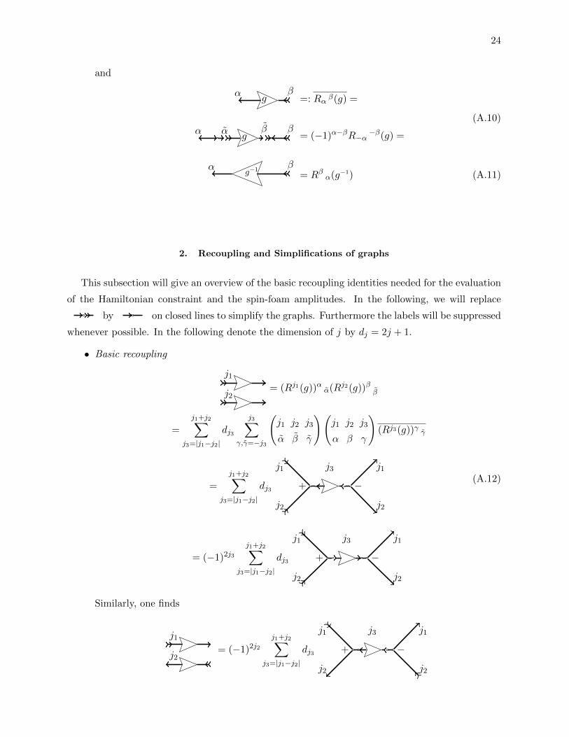
2. Recoupling and Simplifications of graphs

This subsection will give an overview of the basic recoupling identities needed for the evaluation

of the Hamiltonian constraint and the spin-foam amplitudes. In the following, we will replace

by on closed lines to simplify the graphs. Furthermore the labels will be suppressed

whenever possible. In the following denote the dimension of j by dj = 2j + 1.

• Basic recoupling

j1

j2= (Rj1(g))α α(Rj2(g))β β

=

j1+j2∑j3=|j1−j2|

dj3

j3∑γ,γ=−j3

(j1 j2 j3

α β γ

)(j1 j2 j3

α β γ

)(Rj3(g))γ γ

=

j1+j2∑j3=|j1−j2|

dj3 +

j3j1

j2

−j1

j2

= (−1)2j3

j1+j2∑j3=|j1−j2|

dj3 +

j3j1

j2

−j1

j2

(A.12)

Similarly, one finds

j1

j2= (−1)2j2

j1+j2∑j3=|j1−j2|

dj3 +

j3j1

j2

−j1

j2

25

• First orthogonality relation∑α,β

(a b c

α β γ

)(a b c

α β γ

)=

1

dcδc,cδ

γγ

c, γ c, γa

b

=1

dc

γ γc(A.13)

• Six-j-Symbol

++ b

+

af

+

c

e

d

=

{a b c

d e f

}(A.14)

• Second orthogonality relation

∑f

dm df

{a b f

d c e

}{a c m

d b f

}= δem (A.15)

• Summation The following identity is a crucial ingredient for the computation of the matrix

elements of the Hamiltonian operator.∑δ,ε,φ

(−1)d+e+f−δ−ε−φ(d e c

−δ ε γ

)(e f a

−ε φ α

)(f d b

−φ δ β

)

=

{a b c

d e f

}(a b c

α β γ

) (A.16)

Graphically this identity can be encoded in

−

a

b c

− −ef

d

= ++ b

+

af

+

c

e

d

+

a

cb

(A.17)

• Nine-j-Symbol

Definition of a 9j Symbol in terms of 6j’s:

∑x

dx(−1)2x

{a b x

c d p

}{c d x

e f q

}{e f x

a b r

}=

a f r

d q e

p c b

(A.18)

26

Permutation symmetry:

1. j11 j12 j13

j21 j22 j23

j31 j32 j33

= ε

j1i j1j j1k

j2i j2j j2k

j3i j3j j3k

(A.19)

2. j11 j12 j13

j21 j22 j23

j31 j32 j33

= ε

ji1 ji2 ji3

jj1 jj2 jj3

jk1 jk2 jk3

(A.20)

with ε = 1 for even permutations and ε = (−1)R with R =∑

ij jij for odd permutations.

Summation Identity:

∑x

dx

a b e

c d f

e f x

=δbcdbθ(a, b, e)θ(b, d, f) (A.21)

• Integration The matrix elements of the irreducible representations of SU (2) provide an or-

thonormal basis in the space of square integrable functions of SU (2) with respect to the

Haar measure µ(g). This can be visualized by the following diagram:

∫dµ(g) g

α

β

g

α

β

=1

dj

α αj

ββ j(A.22)

The visualization of the integral over higher tensor products works analogously.

• Simplify Graphs From (A.22) follow some useful rules for simplifying graphs. In the following

completely contracted graphs are symbolized by dashed boxes.

j2

j1

= j1δj1,j2dj1

(A.23)

j3

j1

j2 =j2 j2

j3j3

j1 j1

+ − (A.24)

27

The simplification of graphs with more than three edges can be obtained by applying (A.12)

and (A.23) respectively (A.24).

• Sign-Manipulation

Suppose the three irreducible representations a, b, c obey the Clebsch-Gordan conditions then

(a + b + c) ∈ N and thus (−1)2a+2b+2c = 1. This identity is crucial in many calculations in

order to simplify the signs or add missing signs of the form (−1)2a. Since a ∈ 12N we also

have (−1)3a = (−1)−a.

Appendix B: Grasping

A relevant formula used for the computation of the matrix elements of the Hamiltonian in the

4-valent case can be deduced by the double grasping operators on 4-valent nodes, computed in [33]:

+e

b

+

a

+

+

c

d

a′c′

m=

=∑x

(−1)a′+d+e+xdx

{b d x

c′ a′ e

}+

+

b d

+

a

−c

x

a′c′

m

=∑x

(−1)a+c′+x+m(−1)a′+d+e+xdx

{b d x

c′ a′ e

}{c′ a′ x

a c m

}+

+

b d

ac

x

=∑x

(−1)a+c′+x+m(−1)a′+d+e+xdx

∑α

dα(−1)a+d+α+x· (B.1)

·{b d x

c′ a′ e

}{c′ a′ x

a c m

}{b a α

c d x

}+

b

a

+

c

d

α

28

= (−1)b+a−c−d∑α

dα

{e α m

a a′ b

}{e α m

c c′ d

}+

b

a

+

c

d

α(B.2)

Appendix C: Normalization of the spin-network states

Following [2], we define a spin-network S = (Γ, jl, in) as given by a graph Γ with a given

orientation (or ordering of the links) with L links and N nodes, and by a representation jl associated

to each link and an intertwiner in to each node. As a functional of the connection, a spin-network

state is given by

ΨS [A] = 〈A|S〉 ≡(⊗lRjl(h[A, γl])

)x(⊗nin) (C.1)

where x indicates the contraction with the intertwiners and Rjl(h[A, γl]) is the jl representation of

the holonomy group element h[A, γl] along the curve γl of the gravitation field connection A.

The scalar product on Hkin is defined via the Ashtekar-Lewandowski measure:

⟨S|S′

⟩=

∫dµALΨS [A]ΨS [A]

= δS,S′∏e∈E

1

dje

∏v∈V

Tr(ι∗vιv)(C.2)

where E is the set of links and V is the set of vertices of Γ. Throughout this paper we use

normalized intertwiners such that Tr(ι∗vιv) = 1. For a trivalent node this requirement is trivially

fulfilled if we use Wigner 3j-symbols. A higher valent node can be decomposed into trivalent nodes

by introducing virtual links. E.g for a 4-valent node we obtain

√di +

d

a

+

c

b

i(C.3)

If, additionally, we multiply (C.2) by

∏e∈E

√dje

29

we obtain a normalized state |S〉N with respect to (C.2). Consequentially, the recoupling theorem

(B.2) applied to normalized spin-network state yields

∣∣∣ +

d

a

+

c

b

e ⟩N

=∑f

√de√df (−1)b+c+e+f

{a b f

d c e

} ∣∣∣+

a b

+cd

f⟩N

(C.4)

[1] A. Ashtekar, J. Lewandowski, “Background independent quantum gravity: A status report”,

Class. Quant. Grav. 21 R53 (2004).

[2] T. Thiemann, “Modern canonical quantum general relativity”,

(Cambridge University Press, Cambridge, UK, 2007).

[3] C. Rovelli, “Quantum Gravity”, (Cambridge University Press, Cambridge 2004).

[4] P. Dirac, “Lectures on Quantum Mechanics”,

(Belfer Graduate School of Science, Yeshiva University Press,New York 1964).

[5] T. Thiemann, “Quantum spin dynamics (QSD),” Class. Quant. Grav. 15, 839 (1998).

[6] T. Thiemann, “Quantum spin dynamics (QSD) II,” Class. Quant. Grav. 15, 875 (1998).

[7] M. P. Reisenberger, C. Rovelli, “*Sum over surfaces* form of loop quantum gravity,”

Phys. Rev. D 56, 3490 (1997).

[8] A. Perez, “Spin foam models for quantum gravity,” Class. Quant. Grav. 20, R43 (2003),

[arXiv:gr-qc/0301113].

J. Baez, “An introduction to Spinfoam Models of BF Theory and Quantum Gravity”,

Lect.Notes Phys. 543,25-94 (2000), [arXiv:gr-qc/9905087v1].

C. Rovelli, “Zakopane lectures on loop gravity”, (2011), [arXiv:gr-qc/1102.3660].

[9] C. Rovelli, “A new look at loop quantum gravity,” [arXiv:gr-qc/1004.1780].

[10] S. Holst, “Barbero’s Hamiltonian derived from a generalized Hilbert-Palatini action”,

Phys. Rev. D 53, 5966 (1996).

[11] S. Alexandrov, P. Roche, “Critical Overview of Loops and Foams”, (2010),

[arXiv:gr-qc/1009.4475].

[12] J. W. Barrett, L. Crane, “Relativistic spin networks and quantum gravity,”

J. Math. Phys. 39, 3296 (1998), [arXiv:gr-qc/9709028].

J. Barrett, L. Crane, “A Lorentzian Signature Model for Quantum General Relativity”,

Class. Quant. Grav. 17 3101-3118 (2000), [arXiv:gr-qc/9904025].

E. R. Livine, S. Speziale, “A new spinfoam vertex for quantum gravity,”

Phys. Rev. D 76, 084028 (2007).

30

[13] J. Engle, R. Pereira, C. Rovelli, “The loop-quantum-gravity vertex-amplitude,”

Phys. Rev. Lett. 99 (2007) 161301, [arXiv:gr-qc/0705.2388].

J. Engle, R. Pereira, C. Rovelli, “Flipped spinfoam vertex and loop gravity,”

Nucl. Phys. B 798 (2008) 251 .

J. Engle, E. Livine, R. Pereira, C. Rovelli, “LQG vertex with finite Immirzi parameter,”

Nucl. Phys. B 799 (2008) 136 .

L. Freidel, K. Krasnov, “A New Spin Foam Model for 4d Gravity,”

Class. Quant. Grav. 25 (2008) 125018 .

[14] W. Kaminski, M. Kisielowski, J. Lewandowski, “Spin-Foams for All Loop Quantum Gravity,”

Class. Quant. Grav. 27, 095006 (2010).

W. Kaminski, M. Kisielowski, J. Lewandowski, “The EPRL intertwiners and corrected partition func-

tion”, Class. Quant. Grav. 27, 165020 (2010).

[15] K. Noui, A. Perez, “Three dimensional loop quantum gravity: Physical scalar product and spin foam

models,” Class. Quant. Grav. 22, 1739 (2005).

E. Alesci, K. Noui, F. Sardelli, “Spin-Foam Models and the Physical Scalar Product,”

Phys. Rev. D 78, 104009 (2008).

B. Bahr, “On knottings in the physical Hilbert space of LQG as given by the EPRL model”,

Class. Quant. Grav. 28, 045002 (2011), [arXiv:gr-qc/1006.0700].

V. Bonzom, E. Livine, “Yet Another Recursion Relation for the 6j-Symbol”, (2011),

[arXiv:gr-qc/1103.3415].

[16] C. Rovelli, L. Smolin, “Loop Space Representation of Quantum General Relativity,”

Nucl. Phys. B 331, 80 (1990).

C. Rovelli, L. Smolin, “Knot Theory and Quantum Gravity,” Phys. Rev. Lett. 61, 1155 (1988).

[17] C. Rovelli, L. Smolin, “The Physical Hamiltonian in nonperturbative quantum gravity,”

Phys. Rev. Lett. 72, 446 (1994)

[18] C. Rovelli, “Ashtekar formulation of general relativity and loop space nonperturbative quantum gravity:

A Report,” Class. Quant. Grav. 8, 1613 (1991).

V. Husain, “Intersecting loop solutions of the hamiltonian constraint of quantum general relativity”

Nucl. Phys. B 313, 711 (1989).

B. Bruegmann, J. Pullin, “Intersecting N loop solutions of the Hamiltonian constraint of quantum

gravity,” Nucl. Phys. B 363, 221 (1991).

R. Gambini, “Loop space representation of quantum general relativity and the group of loops,”

Phys. Lett. B 255, 180 (1991).

B. Bruegmann, R. Gambini, J. Pullin, “Jones polynomials for intersecting knots as physical states of

quantum gravity,” Nucl. Phys. B 385, 587 (1992).

[19] C. Di Bartolo, R. Gambini, J. Griego, J. Pullin, “Consistent canonical quantization of general relativity

in the space of Vassiliev knot invariants,” Phys. Rev. Lett. 84, 2314 (2000).

R. Gambini, J. Pullin, “Making classical and quantum canonical general relativity computable through

a power series expansion in the inverse cosmological constant,” Phys. Rev. Lett. 85, 5272 (2000).

[20] C. Rovelli, “Outline of a generally covariant quantum field theory and a quantum theory of gravity,”

J. Math. Phys. 36, 6529 (1995).

[21] R. Gambini, J. Lewandowski, D. Marolf, J. Pullin, “On the consistency of the constraint algebra in

spin network quantum gravity,” Int. J. Mod. Phys. D 7, 97 (1998).

31

J. Lewandowski, D. Marolf, “Loop constraints: A habitat and their algebra,”

Int. J. Mod. Phys. D 7, 299 (1998).

L. Smolin, “The classical limit and the form of the Hamiltonian constraint in non-perturbative quantum

general relativity,” [arXiv:gr-qc/9609034].

[22] E. Alesci, C. Rovelli, “A Regularization of the hamiltonian constraint compatible with the spinfoam

dynamics”, Phys. Rev. D 82, 044007 (2010).

[23] J. Lewandowski, “Volume and quantizations,” Class. Quant. Grav. 14, 71 (1997).

[24] C. Rovelli, L. Smolin, “Discreteness of area and volume in quantum gravity,” Nucl. Phys. B 442, 593

(1995) [Erratum-ibid. B 456, 753 (1995)].

[25] A. Ashtekar, J. Lewandowski, “Quantum theory of geometry. II: Volume operators,”

Adv. Theor. Math. Phys. 1, 388 (1998), [arXiv:gr-qc/9711031].

[26] R. De Pietri, C. Rovelli, “Geometry Eigenvalues and Scalar Product from Recoupling Theory in Loop

Quantum Gravity,” Phys. Rev. D 54, 2664 (1996), [arXiv:gr-qc/9602023].

[27] J. Brunnemann, T. Thiemann, “Simplification of the spectral analysis of the volume operator in loop

quantum gravity,” Class. Quant. Grav. 23, 1289 (2006).

[28] M. Gaul, C. Rovelli, “A generalized Hamiltonian constraint operator in loop quantum gravity and its

simplest Euclidean matrix elements,” Class. Quant. Grav. 18, 1593 (2001).

[29] R. Borissov, R. De Pietri, C. Rovelli, “Matrix elements of Thiemann’s Hamiltonian constraint in loop

quantum gravity,” Class. Quant. Grav. 14, 2793 (1997).

[30] C. Rourke, B. Sanderson, “Introduction to Piecewise-Linear Topology”, (Springer Verlag, Berlin 1972).

[31] Y. Ding, M. Han, C. Rovelli, “Generalized Spinfoams”, Phys. Rev. D83, 124020 (2011).

[32] D.M. Brink, G.R. Satchler, “Angular Momentum” 2nd ed., (Clarendon Press, Oxford 1968).

[33] E. Alesci, C. Rovelli, “The complete LQG propagator: I. Difficulties with the Barrett-Crane vertex,”

Phys. Rev. D 76, 104012 (2007).

[34] V. Bonzom, L. Freidel, “The Hamiltonian constraint in 3d Riemannian loop quantum gravity,”

[arXiv:1101.3524 [gr-qc]].

[35] T. Thiemann. “QSD IV: 2+1 Euclidean quantum gravity as a model to test 3+1 Lorentzian quantum

gravity.” Class. Quant. Grav. 15:1249, (1998). [arXiv:gr-qc/9705018]

[36] E. Bianchi, L. Modesto, C. Rovelli and S. Speziale, “Graviton propagator in loop quantum gravity,”

Class. Quant. Grav. 23, 6989 (2006)

E. Alesci and C. Rovelli, “The complete LQG propagator: II. Asymptotic behavior of the vertex,”

Phys. Rev. D 77, 044024 (2008)

E. Alesci, “Tensorial Structure of the LQG graviton propagator,” Int. J. Mod. Phys. A23 (2008)

1209-1213.

E. Alesci, E. Bianchi and C. Rovelli, “LQG propagator: III. The new vertex,” Class. Quant. Grav. 26,

215001 (2009),

E. Bianchi, E. Magliaro and C. Perini, “LQG propagator from the new spin foams,” Nucl. Phys. B

822, 245 (2009).

C. Rovelli, M. Zhang, “Euclidean three-point function in loop and perturbative gravity,”

[arXiv:1105.0566 [gr-qc]].

[37] E. Bianchi, C. Rovelli, F. Vidotto, “Towards Spinfoam Cosmology,” Phys. Rev. D82 (2010) 084035.

[arXiv:1003.3483 [gr-qc]].

32

E. Bianchi, T. Krajewski, C. Rovelli, F. Vidotto, “Cosmological constant in spinfoam cosmology,” Phys.

Rev. D83 (2011) 104015. [arXiv:1101.4049 [gr-qc]].

[38] S. Alexandrov, E. R. Livine, “SU(2) loop quantum gravity seen from covariant theory,” Phys. Rev.

D67 (2003) 044009. [gr-qc/0209105].

[39] V. Bonzom, “Spin foam models and the Wheeler-DeWitt equation for the quantum 4-simplex,” Phys.

Rev. D84 (2011) 024009. [arXiv:1101.1615 [gr-qc]].

[40] K. Giesel and T. Thiemann, “Algebraic Quantum Gravity (AQG) I. Conceptual Setup,” Class. Quant.

Grav. 24, 2465 (2007)

[41] B. Dittrich, P. AHoehn, “Canonical simplicial gravity,” [arXiv:1108.1974 [gr-qc]].