arX

iv:m

ath/

0407

330v

5 [

mat

h.C

A]

9 M

ar 2

006

J. OPERATOR THEORY00:0(0000), 101–144

© Copyright by THETA, 0000

MARTINGALES, ENDOMORPHISMS, AND COVARIANTSYSTEMS OF OPERATORS IN HILBERT SPACE

DORIN ERVIN DUTKAY and PALLE E.T. JORGENSEN

Dedicated to the memory of J.L. Doob

Communicated by S. Stratila

ABSTRACT. In the theory of wavelets, in the study of subshifts, in the analysisof Julia sets of rational maps of a complex variable, and, more generally, inthe study of dynamical systems, we are faced with the problem of building aunitary operator from a mapping r in a compact metric space X. The space Xmay be a torus, or the state space of subshift dynamical systems, or a Julia set.

While our motivation derives from some wavelet problems, we have inmind other applications as well; and the issues involving covariant operatorsystems may be of independent interest.

KEYWORDS: wavelet, Julia set, subshift, Cuntz algebra, iterated function system(IFS), Perron-Frobenius-Ruelle operator, multiresolution, martingale, scaling func-tion, transition probability.

MSC (2000): 47C15, 33C50, 42C15, 42C40, 46E22, 47B32, 60J15, 60G42.

CONTENTS

1. INTRODUCTION 1021.1. Wavelets 1031.2. Examples (Julia sets, subshifts) 1051.3. Martingales 1061.4. The general theory 1062. FUNCTIONS AND MEASURES ON X 1072.1. Transformations of functions and measures 1072.2. Properties of measures µ on X. Definitions 1082.3. Examples 1093. POSITIVE DEFINITE FUNCTIONS AND DILATIONS 1113.1. Operator valued filters 1174. MULTIPLICITY THEORY 1195. PROJECTIVE LIMITS 1236. MARTINGALES 1266.1. Conditional expectations 131

102 DUTKAY AND JORGENSEN

7. INTERTWINING OPERATORS AND COCYCLES 1348. ITERATED FUNCTION SYSTEMS 139REFERENCES 142

1. INTRODUCTION

In this paper, we aim at combining and using ideas from one area of math-ematics (operator theory and traditional analysis) in a different area (martingaletheory from probability). We have in mind applications to both wavelets andsymbolic dynamics. So our paper is interdisciplinary: results in one area oftenbenefit the other. In fact, the benefits go both ways.

Our construction is based on a closer examination of an eigenvalue problemfor a transition operator, also called a Perron-Frobenius-Ruelle operator.

Under suitable conditions on the given filter functions, our constructiontakes place in the Hilbert space L2(Rd). In a variety of examples, for examplefor frequency localized wavelets, more general filter functions are called for. Thisthen entails basis constructions in Hilbert spaces of L2-martingales. These mar-tingale Hilbert spaces consist of L2 functions on certain projective limit spaces X∞

built on a given mapping r : X → X which is onto, and finite-to-one. We studyfunction theory on X∞ in a suitable general framework, as suggested by appli-cations; and we develop our theory in the context of Hilbert space and operatortheory.

We hope that these perhaps unexpected links between more traditional andnarrowly defined fields will inspire further research. Since we wish to reach sev-eral audiences, we have included here a few more details than is perhaps stan-dard in more specialized papers. The general question we address already hasa number of incarnations in the literature, but they have so far not been unified.Here are two such examples which capture the essence of our focus. (a) Extensionof non-invertible endomorphisms in one space X to automorphisms in a biggerspace naturally containing X. (b) Some non-invertible operator S (contractive orisometric) in a fixed Hilbert space H is given. It is assumed that S is contrac-tive and that it satisfies a certain covariance condition specified by a system ofoperators in H. The question is then to extend S to a unitary operator U in a big-ger Hilbert space which naturally contains H, such that U satisfies a covariancecondition arising by dilation from the initially given system on H.

The dilation idea in operator theory is fundamental; i.e., the idea of extend-ing (or dilating) an operator system on a fixed Hilbert space H0 to a bigger ambi-ent Hilbert space H in such a way as to get orthogonality relations in the dilatedspace H; see for example [PaSc72] and Remark 3.3 below. In an operator alge-braic framework such an extension is of course encoded by Stinespring’s theorem

MARTINGALES AND COVARIANT SYSTEMS 103

[Sti55]. Our present setting is motivated by this, but goes beyond it in a numberof ways, as we show in Sections 5–8 below.

Our basic viewpoint may be understood from the example of wavelets: Acrucial strength of wavelet bases is their algorithmic and computational features.What this means in terms of the two Hilbert spaces are three things: First we musthave a concrete function representation of the dilated space H; and secondly weaim for recursive and matrix based algorithms, much like the familiar case ofGram-Schmidt algorithms which lets us compute orthonormal bases, or frames(see e.g., [BJMP05]) in the dilated space H. Thirdly, we reverse the traditionalpoint of view. Hence, the dilation idea is turned around: Starting with H, we wishto select a subspace H0 which is computationally much more feasible. This idea ismotivated by image processing where such a selected subspace H0 correspondsto a chosen resolution, and where "resolution" is to be understood in the sense ofoptics; see e.g., [JMR01] and [Jor06]. The selection of subspace H0 is made in sucha way as to yield recursive algorithms to be used in computation of orthonormalbases, or frames in H, but starting with data from H0.

Examples of (a) occur in thermodynamics, such as it is presented in its rig-orous form by David Ruelle in [Rue89] and [Rue04]. Both (a) and (b) are presentin the approach to wavelets that goes under the name multiresolution analysis(MRA) [Dau92]. In this case, we can take X to be R/Z, or equivalently the cir-cle, or the unit-interval [0, 1), and the extension of X can be taken to be the realline R (see [Dau92]), or it may be a suitable solenoid over X; see, e.g., [BrJo91]and [Bre96]. In this case, the endomorphism in X is multiplication by 2 modulothe integers Z, and the extension to R is simply x → 2x. The more traditionalsettings for (b) are scattering theory [LaPh76] or the theory of extensions, or uni-tary dilations of operators in Hilbert space, as presented for example in [JoMu80],[BMP00], and in the references given there.

Specifically, we study the problem of inducing operators on Hilbert spacefrom non-invertible transformations on compact metric spaces. The operators, orrepresentations must satisfy relations which mirror properties of the given pointtransformations.

While our setup allows a rather general formulation in the context of C∗-algebras, we will emphasize the case of induction from an abelian C∗-algebra.Hence, we will stress the special case when X is a given compact metric space,and r : X → X is a finite-to-one mapping of X onto X. Several of our results arein the measurable category; and in particular we are not assuming continuity ofr, or any contractivity properties.

1.1. WAVELETS. Our results will apply to wavelets. In the theory of multireso-lution wavelets, the problem is to construct a special basis in the Hilbert spaceL2(Rd) from a set of numbers an, n ∈ Zd.

104 DUTKAY AND JORGENSEN

The starting point is the scaling identity

(1.1) ϕ(t) = N1/2 ∑n∈Zd

an ϕ(At− n), (t ∈ Rd),

where A is a d by d matrix over Z, with eigenvalues |λ| > 1, and N = |detA|, andwhere ϕ is a function in L2(Rd).

The first problem is to determine when (1.1) has a solution in L2(Rd), andto establish how these solutions (scaling functions) depend on the coefficients an.

When the Fourier transform is applied, we get the equivalent formulation,

(1.2) ϕ(x) = N−1/2m0(Atr−1x)ϕ(Atr−1

x),

where ϕ denotes the Fourier transform,

ϕ(x) =

∫

Rde−i2πx·tϕ(t) dt

and where now m0 is a function on the torus

Td = z = (z1, ..., zd) ∈ C

d | |zj| = 1, 1 ≤ j ≤ d = Rd/Z

d

, i.e.,m0(z) = ∑

n∈Zd

anzn = ∑n∈Zd

ane−i2πn·x.

The duality between the compact group Td and the lattice Zd is given by

〈 z | n 〉 = zn = zn11 ...znd

d , (z = (z1, ..., zd), n = (n1, ..., nd)).

In this case, matrix multiplication x 7→ Ax on Rd passes to the quotientRd/Zd, and we get an N-to-one mapping x 7→ Ax mod Zd, which we denote byrA.

The function m0 is called a low pass filter, and it is chosen such that theoperator S = Sm0 given by

(S f )(z) = m0(z) f (Az)

is an isometry on H0 = L2(Td, Haar measure). Moreover, L∞(Td) acts as multi-plication operators on H0. If g ∈ L∞(T)

(M(g) f )(z) = g(z) f (z)

and

(1.3) SM(g) = M(g(A·))S

A main problem is the extension of this covariance relation (1.3) to a bigger Hilbertspace H0 → Hext, S→ Sext, such that Sext is unitary in Hext. We now sketch brieflythis extension in some concrete cases of interest.

In Section 5, we construct a sequence of measures ω0, ω1, ... on Td such thatL2(Td, ω0) ≃ H0, and such that there are natural isometric embeddings

(1.4) L2(Td, ωn) → L2(Td, ωn+1), f 7→ f rA.

MARTINGALES AND COVARIANT SYSTEMS 105

The limit in (1.4) defines a martingale Hilbert space H in such a way that the normof the L2-martingale f is

‖ f ‖2 = limn→∞

‖Pn f ‖2L2(Td,ωn)

We also state a pointwise a.e. convergence result (Section 6).If Ψ : L2(Td, ωn)→ L2(Rd) is defined by

Ψ : fn 7→ fn(A−nx)ϕ(x),

then Ψ is an isometry of L2(Td, ωn) into L2(Rd).Specifically

(1.5)∫

Td| fn|2 dωn =

∫

Rd| fn(A−nx)ϕ(x)|2 dx

As a result we have induced a system

(rA , Td)→ (Sm0 , L2(Td)) → (UA, L2(Rd)).

where

(1.6) (UAξ)(x) = N1/2 f (Ax), ( f ∈ L2(Rd))

UA unitary; the system is determined by the given filter function m0. It can bechecked (see details in Section 6) that Ψ is an isometry, and that

UA M(g) = M(g(A·))UA

holds on L2(Rd). Moreover Ψ maps onto L2(Rd) if the function m0 doesn’t vanishon a subset of positive measure.

In the case of wavelets, we ask for a wavelet basis in L2(Rd) which is consis-tent with a suitable resolution subspace in L2(Rd). Whether the basis is orthonor-mal, or just a Parseval frame, it may be constructed from a system of subbandfilters mi, say with N frequency bands. These filters mi may be realized as func-tions on X = Td = Rd/Zd, the d-torus. Typically the scaling operation is specifiedby a given expansive integral d by d matrix A.

Let N := |detA|. Pass A to the quotient X = Rd/Zd, and we get a mapping r

of X onto X such that #r−1(x) = N for all x in X, and the N branches of the inverseare strictly contractive in X = Rd/Zd if the eigenvalues of A satisfy |λ| > 1.

The subband filters mi are defined in terms of this map, rA, and the problemis now to realize the wavelet data in the Hilbert space L2(Rd) in such a way thatr = rA : X → X induces the unitary scaling operator f 7→ N1/2 f (Ax) in L2(Rd),see (1.6).

1.2. EXAMPLES (JULIA SETS, SUBSHIFTS). In this paper we will show that thisextension from spaces X, with a finite-to-one mapping r : X → X, to operatorsystems may be done quite generally, to apply to the case when X is a Julia setfor a fixed rational function of a complex variable, i.e., r(z) = p1(z)/p2(z), withp1, p2 polynomials, z ∈ C and N = max(deg p1, deg p2). Then r : X(r) → X(r))is N-to-1 except at the singular points of r. Here X(r) denotes the Julia set of r.

106 DUTKAY AND JORGENSEN

It also applies to shift invariant spaces X(A) when A is a 0− 1 matrix, and

X(A) = (xi) ∈∏N

1, ..., N | A(xi, xi+1) = 1

andrA(x1, x2, ...) = (x2, x3, ...)

is the familiar subshift. Note that rA : X(A) → X(A) is onto iff every column inA contains at least one entry 1.

1.3. MARTINGALES. Part of the motivation for our paper derives from the pa-pers by Richard Gundy [Gun00], [Gun04], [Gun99], [Gun66]. The second namedauthor also acknowledges enlightening discussions with R. Gundy. The funda-mental idea in these papers by Gundy et al is that multiresolutions should beunderstood as martingales in the sense of Doob [Doob1],[Doob2],[Doob3] andNeveu [Neveu]. And moreover that this is a natural viewpoint.

One substantial advantage of this viewpoint is that we are then able to han-dle the construction of wavelets from subband filters that are only assumed mea-surable, i.e., filters that fail to satisfy the regularity conditions that are tradition-ally imposed in wavelet analysis.

A second advantage is that the martingale approach applies to a numberof wavelet-like constructions completely outside the traditional scope of wave-let analysis in the Hilbert space L2(Rd). But more importantly, the martingaletools apply even when the operation of scaling doesn’t take place in Rd at all,but rather in a compact Julia set from complex dynamics; or the scaling opera-tion may be one of the shift in the subshift dynamics that is understood from thatthermodynamical formalism of David Ruelle [Rue89].

1.4. THE GENERAL THEORY. In each of the examples, we are faced with a givenspace X, and a finite-to-one mapping r : X → X. The space X is equipped witha suitable family of measures µh, and the L∞ functions on X act by multiplica-tion on the corresponding L2 spaces, L2(X, µh). It is easy to see that there are L2

isometries which intertwine the multiplication operators M(g) and M(g r), as granges over L∞(X). We have

(1.7)

L2(X, µh)S−→ L2(X, µh)

↓

↓

HextU−→ Hext

where the vertical maps are given by inclusions. Specifically,

(1.8) SM(g) = M(g r)S, and UM(g)U−1 = M(g r)

But for spectral theoretic calculations, we need to have representations ofM(g) and M(g r) unitarily equivalent. That is true in traditional wavelet appli-cations, but the unitary operator U in (1.8) is not acting on L2(X, µh). Rather, the

MARTINGALES AND COVARIANT SYSTEMS 107

unitary U is acting by matrix scaling on a different Hilbert space, namelyL2(Rd, Lebesgue measure),

UA f (t) = | det A|1/2 f (At), (t ∈ Rd, f ∈ L2(Rd).

In the other applications, Julia set, and shift-spaces, we aim for a similarconstruction. But in these other cases, it is not at all clear what the Hilbert spacecorresponding to L2(Rd), and the corresponding unitary matrix scaling operator,should be.

We provide two answers to this question, one at an abstract level, and asecond one which is a concrete function representation; Sections 4 and 5.

At the abstract level, we show that the construction may be accomplishedin Hilbert spaces which serve as unitary dilations of the initial structure, see (1.7).

In the concrete, we show that the extended Hilbert spaces may be taken asHilbert spaces of L2- martingales on X. In fact, we present these as Hilbert spacesof L2 functions built from a projective limit

Xr← X

r← X....← X∞.

This is analogous to the distinction between an abstract spectral theorem on theone hand, and a concrete spectral representation, on the other. To know detailsabout multiplicities, and multiplicity functions (Section 4), we need the latter.

Our concrete version of the dilation Hilbert space Hext from (1.7) is then

Hext ≃ L2(X∞, µh)

for a suitable measure µh on X∞.

2. FUNCTIONS AND MEASURES ON X

Consider

• X a compact metric space,• B = B(X) a Borel sigma-algebra of subsets of X,• r : X → X an onto, measurable map such that #r−1(x) < ∞ for all x ∈ X,• W : X → [0, ∞),• µ a positive Borel measure on X.

2.1. TRANSFORMATIONS OF FUNCTIONS AND MEASURES.

• Let g ∈ L∞(X). Then

(2.1) M(g) f = g f

is the multiplication operator on L∞(X) or on L2(X, µ).• Composition:

(2.2) S0 f = f r, or (S0 f )(x) = f (r(x)), (x ∈ X).

108 DUTKAY AND JORGENSEN

• If m0 ∈ L∞(X), we set

Sm0 = M(m0)S0,

or equivalently

(2.3) (Sm0 f )(x) = m0(x) f (r(x)), (x ∈ X, f ∈ L∞(X)).

• r−1(E) := x ∈ X | r(x) ∈ E for E ∈ B(X).

µ r−1(E) = µ(r−1(E)), (E ∈ B(X)).

2.2. PROPERTIES OF MEASURES µ ON X. DEFINITIONS.

(i) Invariance:

(2.4) µ r−1 = µ.

(ii) Strong invariance:

(2.5)∫

Xf (x) dµ =

∫

X

1#r−1(x)

∑r(y)=x

f (y) dµ, ( f ∈ L∞(X)).

(iii) W : X → [0, ∞),

(2.6) (RW f )(x) = ∑r(y)=x

W(y) f (y).

If m0 ∈ L∞(X, µ) is complex valued, we use the notation Rm0 := RW

where W(x) = |m0(x)|2/#r−1(r(x)).(a) A function h : X → [0, ∞) is said to be an eigenfunction for RW if

(2.7) RWh = h

(b) A Borel measure ν on X is said to be a left-eigenfunction for RW if

(2.8) νRW = ν,

or equivalently∫

XRW f dν =

∫

Xf dν, for all f ∈ L∞(X).

LEMMA 2.1. (i) For measures µ on X we have the implication (2.5)⇒ (2.4),but not conversely.

(ii) If W is given and if ν and h satisfy (2.8) and (2.7) respectively, then

(2.9) dµ := h dν

satisfies (2.4).(iii) If µ satisfies (2.5), and m0 ∈ L∞(X), then Sm0 is an isometry in L2(X, h dµ) if

and only if

Rm0 h = h.

MARTINGALES AND COVARIANT SYSTEMS 109

Proof. (i) Suppose µ satisfies (2.5). Let f ∈ L∞(X). Then∫

Xf r dµ =

∫

X

1#r−1(x)

∑r(y)=x

f (r(y)) dµ(x) =

∫

Xf dµ.

(ii) Let W, ν and h be as in the statement of part (ii) of the lemma. Then∫

Xf r dµ =

∫

Xf r h dν =

∫

XRW( f r h) dν

=

∫

Xf RWh dν =

∫

Xf h dν =

∫

Xf dµ,

which is the desired conclusion (2.4). It follows in particular that (2.5) is strictlystronger than (2.4).

(iii) For f ∈ L∞(X), we have

‖Sm0 f ‖2L2(X,h dµ) =

∫

X|m0(x) f (rx)|2h(x) dµ

=

∫

X| f (x)|2 1

#r−1(x) ∑r(y)=x

|m0(y)|2h(y) dµ(x)

=

∫

X| f (x)|2Rm0 h(x) dµ(x) =

∫

X| f |2h dµ = ‖ f ‖2

L2(X,h dµ)

iff Rm0 h = h and (iii) follows.

We will use standard facts from measure theory: for example, we may iden-tify positive Borel measures on X with positive linear functionals on C(X) via

Λω( f ) =

∫

Xf dω.

In fact, we will identify Λω and ω. For two measures µ and ν on X, we will usethe notation µ ≺ ν to denote absolute continuity. For example µ ≺ ν holds in(2.9).

2.3. EXAMPLES. We illustrate the definitions:

EXAMPLE 2.2. Let X = [0, 1] = R/Z. Fix N ∈ Z+, N > 1. Let

r(x) = Nx mod 1

Invariance:

(2.10)∫ 1

0f (Nx) dµ(x) =

∫ 1

0f (x) dµ(x), ( f ∈ L∞(R/Z)).

Strong invariance:

(2.11)1N

∫ 1

0

N−1

∑k=0

f

(

x + k

N

)

dµ(x) =

∫ 1

0f (x) dµ(x).

The Lebesgue measure µ = λ is the unique probability measure on [0, 1] =

R/Z which satisfies (2.11).

110 DUTKAY AND JORGENSEN

Examples of measures µ on R/Z which satisfy (2.10) but not (2.11) are

• µ = δ0, the Dirac mass at x = 0;• µ = µC, the Cantor middle-third measure on [0, 1] (see [DutJo]), i.e., µC

is determined by–

12

∫ (

f(

x3

)

+ f(

x+23

))

dµC(x) =∫

f (x) dµC(x),– µC([0, 1]) = 1,– µC is supported on the middle-third Cantor set.

EXAMPLE 2.3. Let X = [0, 1) = R/Z, λ the Lebesgue measure, XC themiddle-third Cantor set, µC the Cantor measure.

r : X → X, r(x) = 3x mod 1, rC = rXC: XC → XC.

Consider the following properties for a Borel probability measure µ on R:

(2.12)∫

f dµ =13

∫ (

f (x

3) + f (

x + 13

) + f (x + 2

3)

)

dµ(x);

(2.13)∫

f dµ =12

∫(

f (x

3) + f (

x + 23

)

)

dµ(x);

Then (2.12) has a unique solution µ = λ. Moreover (2.13) has a unique solution,µ = µC, and µC is supported on the Cantor set XC.

Let R/Z = [0, 1). Then #r−1(x) = 3 for all x ∈ [0, 1). If x = x13 + x2

32 + ...,xi ∈ 0, 1, 2, is the representation of x in base 3, then r(x) ∼ (x2, x3, ...), andr−1(x) = (0, x1, x2, ...), (1, x1, x2, ...), (2, x1, x2, ...)

On the Cantor set #r−1C

(x) = 2 for all x ∈ XC. If x = x13 + x2

32 + ..., xi ∈ 0, 2is the usual representation of XC in base 3, then

rC(x) = (x2, x3, ...)

and

XC ≃∏N

0, 2.

In the representation ∏N Z3 of X = [0, 1), µ = λ is the product (Bernoulli)measure with weights ( 1

3 , 13 , 1

3 ).In the representation ∏N0, 2 of XC, µC is the product (Bernoulli) measure

with weights ( 12 , 1

2 ).

EXAMPLE 2.4. Let N ∈ Z+, N ≥ 2 and let A = (aij)Ni,j=1 be an N by N matrix

with all aij ∈ 0, 1. Set

X(A) := (xi) ∈∏N

1, ..., N | A(xi, xi+1) = 1

and let r = rA be the restriction of the shift to X(A), i.e.,

rA(x1, x2, ...) = (x2, x3, ...), (x = (x1, x2, ...) ∈ X(A)).

MARTINGALES AND COVARIANT SYSTEMS 111

LEMMA 2.5. Let A be as above. Then

#r−1A (x) = #y ∈ 1, ..., N | A(y, x1) = 1.

It follows that rA : X(A) → X(A) is onto iff A is irreducible, i.e., iff for allj ∈ ZN , there exists an i ∈ ZN such that A(i, j) = 1.

Suppose in addition that A is aperiodic, i.e., there exists p ∈ Z+ such thatAp

> 0 on ZN ×ZN . We have the following lemma:

LEMMA 2.6 (D. Ruelle, [Rue89], [Bal00]). Let A be irreducible and aperiodic and

let φ ∈ C(X(A)) be given. Assume that φ is a Lipschitz function.

(i) Set

(Rφ f )(x) = ∑rA(y)=x

eφ(y) f (y), for f ∈ C(X(A)).

Then there exist λ0 > 0„

λ0 = sup|λ| | λ ∈ spec(Rφ),

h ∈ C(X(A)) strictly positive and ν a Borel measure on X(A) such that

Rφh = λ0h,

νRφ = λ0ν,

and ν(h) = 1. The data is unique.

(ii) In particular, setting

(R0 f )(x) =1

#r−1A (x)

∑rA(y)=x

f (y),

we may take λ0 = 1, h = 1 and ν =: µA, where µA is a probability measure on

X(A) satisfying the strong invariance property∫

X(A)f dµA =

∫

X(A)

1

#r−1A (x)

∑rA(y)=x

f (y) dµA(x), ( f ∈ L∞(X(A)).

3. POSITIVE DEFINITE FUNCTIONS AND DILATIONS

We now recall a result relating operator systems to positive definite func-tions. The idea dates back to Kolmogorov, but has been used recently in for ex-ample [FO00] and [Dut3] (see also [Aro]).

DEFINITION 3.1. A map K : X × X → C is called positive definite if, for anyx1, .., xn ∈ X and any ξ1, ..., ξn ∈ C,

n

∑i,j=1

K(xi, xj)ξ iξ j ≥ 0.

112 DUTKAY AND JORGENSEN

THEOREM 3.2 (Kolmogorov-Aronszajn). Let K : X × X → C be positive defi-

nite. Then there exist a Hilbert space and a map v : X → H such that

spanv(x) | x ∈ X = H,

〈 v(x) | v(y) 〉 = K(x, y), (x, y ∈ X).

Moreover H and v are unique up to isomorphism.

Proof. We sketch the idea of the proof. Take H to be the completion of thespace

f : X → C | f has finite support with respect to the scalar product

〈 f | g 〉 = ∑x,y∈X

f (x)K(x, y)g(y).

Then define v(x) := δx.

REMARK 3.3. Theorem 3.2 has a long history in operator theory. The versionabove is purely geometric, but as noted, for example in [PaSc72] and [BCR84], itis possible to take the Hilbert space H in the theorem of the form L2(Ω, B, µ)

where (Ω, B, µ) is a probability space; i.e., B is a sigma-algebra on some measurespace Ω, µ a measure defined on B, µ(Ω) = 1. In that case, v(x, .) is a stochasticprocess. As is well known, it is even possible to make this choice such that theprocess is Gaussian. Examples of this include Brownian motion, and fractionalBrownian motion, see also [Moh03], [Aya04], [JMR01]; – and [MoPa92] for a moreoperator theoretic approach.

For the purpose of the present discussion, it will be enough to know theHilbert space H abstractly, but in the main part of our paper (Sections 5–8), theparticular function representation will be of significance. To see this, take forexample the case of the more familiar wavelet construction from Example 1.1above. In the present framework, the space X is then the d-torus Td, while theambient dilation Hilbert space H is L2(Rd). Since wavelet bases must be realizedin the ambient Hilbert space, it is significant to have much more detail than isencoded in the purely geometric data of Theorem 3.2. Even when comparingwith the function theoretic version of [PaSc72], the wavelet example illustratesthat it is significant to go beyond probability spaces.

One of our aims is to offer a framework for more general wavelet bases,including state spaces in symbolic dynamics and Julia sets (such as [BrTo05].) Amain reason for the usefulness of wavelet bases is their computational features.As is well known [San59], there are many function theoretic orthonormal bases(ONB), or Parseval frames in analysis where the basis coefficients do not lendthemselves practical algorithmic schemes. If for example we are in L2(Rd), thenthe computation of each basis coefficients typically involves a separate integra-tion over Rd; not at all a computationally attractive proposition.

MARTINGALES AND COVARIANT SYSTEMS 113

What our present approach does is that it selects a subspace of the ambi-ent Hilbert space which is computationally much more feasible. As stressed in[BJMP05] and [Jor06], such a selection corresponds to a choice of resolution, a no-tion from optics; and one dictated in turn by applications. In the present setup,the chosen resolution corresponds to an initial space, which in this context maybe encoded by X from Theorem 3.2 above. As we will see later, there are waysto do this in such that the computation of basis coefficients becomes algorithmic.We will talk about wavelet bases in this much more general contest, even thoughwavelets are traditionally considered only in L2(Rd). With good choices, we findthat computation of the corresponding basis coefficients may be carried with acertain recursive algorithms involving only matrix iteration; much like in the fa-miliar case of Gram-Schmidt algorithms.

THEOREM 3.4. Let K be a positive definite map on a set X. Let s : X → X be amap that is compatible with K in the sense that

(3.1) K(s(x), s(y)) = K(x, y), (x, y ∈ X).

Then there exists a Hilbert space H, a map v : X → H and a unitary operator U on Hsuch that

(3.2) 〈 v(x) | v(y) 〉 = K(x, y), (x, y ∈ X),

(3.3) spanU−n(v(x)) | x ∈ X, n ≥ 0 = H,

(3.4) Uv(x) = v(s(x)), (x ∈ X).

Moreover, this is unique up to an intertwining isomorphism.

Proof. Let X := X ×Z. Define K : X × X → C by

K((x, n), (y, m)) = K(sn+M(x), sm+M(y)), (x, y ∈ X, n, m ∈ Z),

where M ≥ max−m,−n.The compatibility condition (3.1) implies that the definition does not de-

pend on the choice of M. We check that K is positive definite. Take (xi, ni) ∈ X

and ξi ∈ C. Then, for M big enough we have:

∑i,j

K((xi, ni), (xj, nj))ξ iξ j = ∑i,j

K(sM+ni(xi), sM+nj(xj))ξ iξ j ≥ 0.

Using now the Kolmogorov construction (see Theorem 3.2), there exists a Hilbertspace H and a map v : X → H such that

〈 v(x, n) | v(y, m) 〉 = K((x, n), (y, m)), ((x, m), (y, n) ∈ X),

spanv(x, m) | (x, m) ∈ X = H.

Define v byv(x) = v(x, 0), (x ∈ X).

114 DUTKAY AND JORGENSEN

Then (3.2) is satisfied. Define

Uv(x, n) = v(x, n + 1), ((xn) ∈ X).

U is well defined and an isometry because, for M sufficiently big,

〈 v(x, n + 1) | v(y, m + 1) 〉 = K(sM+n+1(x), sM+m+1(y))

= K(sM+n(x), sM+m(y)) = 〈 v(x, n) | v(y, m) 〉 .U has dense range so U is unitary. Also (3.3) is immediate (we need only n ≥ 0because Un(v(x)) = v(sn(x)), for n ≥ 0, will follow form (3.4)).

For (3.4) we compute

〈Uv(x) | v(y, n) 〉 = K((x, 1), (y, n)) = K(sM+1(x), sM+n(y))

= K(sM(s(x)), sM+n(y)) = 〈 v(s(x)) | v(y, n) 〉 .

For uniqueness, if H′, v′, U ′ satisfy the same conditions, then the formulaW(Unv(x)) = U ′nv′(x) defines an intertwining isomorphism.

THEOREM 3.5. Let A be a unital C∗-algebra, α an endomorphism on A, µ a state

on A and, m0 ∈ A, such that

(3.5) µ(m∗0α( f )m0) = µ( f ), ( f ∈ A).

Then there exists a Hilbert space H, a representation π of A on H, U a unitary on H,and a vector ϕ ∈ A, with the following properties:

(3.6) Uπ( f )U∗ = π(α( f )), ( f ∈ A),

(3.7) 〈 ϕ | π( f )ϕ 〉 = µ( f ), ( f ∈ A),

(3.8) Uϕ = π(α(1)m0)ϕ

(3.9) spanU−nπ( f )ϕ | n ≥ 0, f ∈ A = H.

Moreover, this is unique up to an intertwining isomorphism.We call (H, U, π, ϕ) the covariant system associated to µ and m0.

Proof. Define K and s by

K(x, y) = µ(x∗y), s(x) = α(x)m0, (x, y ∈ A).

K is positive definite and compatible with s so, with Theorem 3.4, there existsa Hilbert space H, a map v from A to H, and a unitary U with the mentionedproperties.

Define ϕ = v(1),

π( f )(U−nv(x)) = U−nv(αn( f )x), ( f , x ∈ A, n ≥ 0).

MARTINGALES AND COVARIANT SYSTEMS 115

Some straightforward computations show that π is a well defined representationof A that satisfies all requirements.

COROLLARY 3.6. Let X be a measure space, r : X → X a measurable, onto mapand µ a probability measure on X such that

(3.10)∫

Xf dµ =

∫

X

1#r−1(x) ∑

r(y)=x

f (y) dµ(x).

Let h ∈ L1(X), h ≥ 0 such that

1#r−1(x)

∑r(y)=x

|m0(y)|2h(y) = h(x), (x ∈ X).

Then there exists (uniquely up to isomorphisms) a Hilbert space H, a unitary U, a repre-sentation π of L∞(X) and a vector ϕ ∈ H such that

Uπ( f )U−1 = π( f r), ( f ∈ L∞(X)),

〈 ϕ | π( f )ϕ 〉 =

∫

Xf h dµ, ( f ∈ L∞(X)),

Uϕ = π(m0)ϕ,

spanU−nπ( f )ϕ | n ≥ 0, f ∈ L∞(X) = H.

We call (H, U, π, ϕ) the covariant system associated to m0 and h.

Proof. Take µ( f ) =∫

X f h dµ, α( f ) = f r; and use Theorem 3.5.

We regard Theorem 3.5 as a dilation result. In this context we have a secondclosely related result:

THEOREM 3.7. (i) Let H be a Hilbert space, S an isometry on H. Then there exist

a Hilbert space H containing H and a unitary S on H such that

(3.11) S|H = S,

(3.12)⋃

n≥0

S−nH = H.

Moreover these are unique up to an intertwining isomorphism.

(ii) If A is a C∗-algebra, α is an endomorphism on A and π is a representation ofA on H such that

(3.13) Sπ(g) = π(α(g))S, (g ∈ A);

then there exists a unique representation π on H such that

(3.14) π(g)|H = π(g), (g ∈ A),

116 DUTKAY AND JORGENSEN

(3.15) Sπ(g) = π(α(g))S, (g ∈ A).

Proof. (i) Consider the set of symbols

Hsym := ∑j∈Z

Sjξ j | ξ j ∈ H, ξ j = 0 except for finiteley many j’s.

Define the scalar product

(3.16)

⟨

∑i∈Z

Siξi

∣

∣

∣ ∑j∈Z

Sjηj

⟩

= ∑i,j∈Z

⟨

Si+mξi

∣

∣ Sj+mηj

⟩

,

where m is chosen sufficiently large, such that i + m, j + m ≥ 0 for all i, j ∈ Z withξi 6= 0, ηj 6= 0.

Since S is an isometry this definition does not depend on the choice of m.We denote the completion of Hsym with this scalar product by H. H can be iso-metrically identified with a subspace of H by

ξ 7→ ∑i∈Z

Siξi, where ξi =

0 if i 6= 0ξ if i = 0.

Define

S(∑i∈Z

Siξi) = ∑i∈Z

Si+1ξi.

In the definition of H, we use (3.16) as an inner product, and we set

H =

(

Hsym/∑j

Sjξ j | ∑i,j

⟨

Si+mξi

∣

∣ Sj+mξ j

⟩

= 0)∧

where ∧ stands for completion.Since ξ = S−1(Sξ) in Hsym, for ξ ∈ H, we get natural isometric embeddings

as follows, see (3.12),

H ⊂ S−1H ⊂ S−2H ⊂ ... ⊂ S−nH ⊂ S−n−1H ⊂ ...

It can be checked that H and S satisfy the requirements.(ii) We know that the spaces

S−nξ | n ≥ 0, ξ ∈ H

span a dense subspace of H. Define

π(g)(S−nξ) = S−nπ(αn(g))ξ, (g ∈ A, n ≥ 0, ξ ∈ H).

MARTINGALES AND COVARIANT SYSTEMS 117

We check only that π(g) is a well defined, bounded operator, the rest of our claimsfollow from some elementary computations. Take m large:

‖π(g)(∑i

S−ni ξi)‖2 = ‖∑i

S−niπ(αni (g))ξi‖2

= ‖∑i

Sm−niπ(αni (g))ξi‖2

= ‖∑i

π(αm(g))Sm−ni ξi‖2

≤ ‖g‖2‖∑i

S−ni ξi‖2.

EXAMPLE 3.8. This example is from [BCMO], and it illustrates the conclu-sions in Theorem 3.7.

Consider1. H = l2(N0),2. S(c0, c1, ..) = (c1, c2, ...), the unilateral shift,3. δk(j) = δk,j = Kronecker delta, for k, j ∈ N0,4. π(gk)δj := exp(i2πk2−j)δj, j ∈ N0, k ∈ Z[1/2].

When Theorem 3.7 is applied we get:1’. The dilation Hilbert space H is l2(Z).2’. S is the bilateral shift on l2(Z) i.e., Sδj = δj−1 for j ∈ Z.3’. Same as in 3. but for k, j ∈ Z.4’. The operator π(gk) is given by the same formula 4., but for j ∈ Z.

The commutation relation (3.15) now takes the form

(3.17) Sπ(gk) = π(g2−1k)S on l2(Z), for k ∈ Z[1/2];

and

(3.18) S−nH = spanδ−n, δ−n+1, δ−n+2, ... ⊂ H.

3.1. OPERATOR VALUED FILTERS. In this subsection we study the multiplicityconfigurations of the representations π from above. Our first result shows thatthe two functions m0, and h in Section 2.1 may be operator valued. The explicitmultiplicity functions are then calculated in the next section.

COROLLARY 3.9. Let X, r, and µ be as in Corollary 3.6. Let I be a finite or count-

able set. Suppose H : X → B(l2(I)) has the property that H(x) ≥ 0 for almost ev-

ery x ∈ X, and Hij ∈ L1(X) for all i, j ∈ I. Let M0 : X → B(l2(I)) such that

x 7→ ‖M0(x)‖ is essentially bounded. Assume in addition that

(3.19)1

#r−1(x)∑

r(y)=x

M∗0(y)H(y)M0(y) = H(x), for a.e. x ∈ X.

118 DUTKAY AND JORGENSEN

Then there exists a Hilbert space K, a unitary operator U on K, a representation π of

L∞(X) on K, and a family of vectors (ϕi) ∈ K, such that:

Uπ(g)U−1 = π(g r), (g ∈ L∞(X)),

Uϕi = ∑j∈I

π((M0)ji)ϕj, (i ∈ I),

⟨

ϕi | π( f )ϕj

⟩

=

∫

Xf Hij dµ, (i, j ∈ I, f ∈ L∞(X)),

spanπ( f )ϕi | n ≥ 0, f ∈ L∞(X), i ∈ I = K.

These are unique up to an intertwining unitary isomorphism. (All functions are assumed

weakly measurable in the sense that x 7→ 〈 ξ | F(x)η 〉 is measurable for all ξ, η ∈ l2(I).)

Proof. Consider the Hilbert space

K := f : X → CI | f is measurable ,

∫

X〈 f (x) | H(x) f (x) 〉 dµ(x) < ∞.

Define S on K by

(S f )(x) = M0(x)( f (r(x))), (x ∈ X, f ∈ K).

We check that S is an isometry. For f , g ∈ K:

〈 Sg | S f 〉 =

∫

X〈M0(x)g(r(x)) | H(x)M0(x) f (r(x)) 〉 dµ(x)

=

∫

X〈 g(r(x)) | M0(x)∗H(x)M0(x) f (r(x)) 〉 dµ(x)

=

∫

X

1#r−1(x)

∑r(y)=x

〈 g(x) | M0(y)∗H(y)M0(y) f (x) 〉 dµ(x)

=

∫

X〈 g(x) | H(x) f (x) 〉 dµ(x) = 〈 g | f 〉 ,

where we used (3.19) in the last step. The converse implication holds as well, i.e.,if S is an isometry then (3.19) is satisfied.

Define now

(π(g) f )(x) = g(x) f (x), (x ∈ X, g ∈ L∞(X), f ∈ K).

π defines a representation of L∞(X) on K. Moreover, the covariance relation issatisfied

Sπ(g) = π(g r)S.

Then we use Theorem 3.7 to obtain a Hilbert space K containing K, a unitaryU := S on K, and a representation π on K that dilate S and π.

Define ϕi ∈ K ⊂ K,

ϕi(x) := δi, for all x ∈ X, (i ∈ I).

MARTINGALES AND COVARIANT SYSTEMS 119

We have that⟨

ϕi | π( f )ϕj

⟩

=

∫

X

⟨

δi | H(x)( f (x)δj)⟩

dµ(x) =

∫

Xf (x)Hij(x) dµ(x),

(Uϕi)(x) = (Sϕi)(x) = M0(x)δi = ((M0)ji(x))j∈I = (∑j∈I

π((M0)ji)ϕj)(x).

Also it is clear that

spanπ( f )ϕi | f ∈ L∞(X), i ∈ I = K.

These relations, together with Theorem 3.7, prove our assertions.

4. MULTIPLICITY THEORY

One of the tools from operator theory which has been especially useful inthe analysis of wavelets is multiplicity theory for abelian C∗-algebrasA.

We first recall a few well known facts, see e.g., [N]. By Gelfand’s theo-rem, every abelian C∗-algebra with unit is C(X) for a compact Hausdorff spaceX; and every representation of A is the orthogonal sum of cyclic representations.While the cardinality of the set of cyclic components in this decomposition is aninvariant, the explicit determination of the cyclic components is problematic, asthe construction depends on Zorn’s lemma. So for this reason, it is desirable toturn the abstract spectral theorem for representations into a concrete one. In theconcrete spectral representation, C(X) is represented as an algebra of multiplica-tion operators on a suitable L2-space; as opposed to merely an abstract Hilbertspace. When we further restrict attention to normal representations of A, we willbe working with the algebra L∞(X) defined relative to the Borel sigma-algebra ofsubsets in X.

With this, we are able to compute a concrete spectral representation, andthereby to strengthen the conclusion from Theorem 3.7.

Our L2-space which carries the representation may be realized concretelywhen the additional structure from Section 2.1 is introduced, i.e., is added to theassumptions in Theorem 3.7. Hence, we will work with the given finite-to-onemapping r : X → X, and the measure µ from before. Recall from Section 2 that µ

is assumed strongly r-invariant.Theorem 3.7 provides an abstract unitary dilation of a given covariant sys-

tem involving a representation π and a fixed isometry S on a Hilbert space H.In the present section, we specialize the representation π in Theorem 3.7 to thealgebra A = L∞(X), and α : A → A, is α(g) := g r.

While our conclusion from Theorem 3.7 still offers a unitary dilation U inan abstract Hilbert space H, we are now able to show that H has a concrete spec-tral representation. Since H is the closure of an ascending union of resolutionsubspaces defined from U, the question arises as to how the multiplicities of

120 DUTKAY AND JORGENSEN

the restricted representations of the resolution subspaces in H are related to one-another.

The answer to this is known in the case of wavelets, see e.g., [BM]. In thissection we show that there is a version of the Baggett et al multiplicity formula inthe much more general setting of Theorem 3.7. In particular, we get the multiplic-ity formula in the applications where X is a Julia set, or a state space of sub-shiftdynamical system. As we noted in Section 2 above, each of these examples carriesa natural mapping r, and a strongly r-invariant measure µ.

Consider X a measure space, r : X → X an onto, measurable map such that#r−1(x) < ∞ for all x ∈ X. Let µ be a measure on X such that

(4.1)∫

Xf dµ =

∫

X

1#r−1(x) ∑

r(y)=x

f (y) dµ(x), ( f ∈ L∞(X)).

Suppose now that H is a Hilbert space with an isometry S on it and with anormal representation π of L∞(X) on H that satisfies the covariance relation

(4.2) Sπ(g) = π(g r)S, (g ∈ L∞(X)).

Theorem 3.7 shows that there exists a Hilbert space H containing H, a uni-tary S on H and a representation π of L∞(X) on H such that:

(Vn := S−n(H))n form an increasing sequence of subspaces with dense union,

S|H = S,

π|H = π,

Sπ(g) = π(g r)S.

THEOREM 4.1. (i) V1 = S−1(H) is invariant for the representation π. The mul-

tiplicity functions of the representation π on V1, and on V0 = H, are related by

(4.3) mV1(x) = ∑r(y)=x

mV0(y), (x ∈ X).

(ii) If W0 := V1 ⊖V0 = S−1H ⊖ H, then

(4.4) mV0(x) + mW0(x) = ∑r(y)=x

mV0(y), (x ∈ X).

Proof. Note that S maps V1 to V0, and the covariance relation implies thatthe representation π on V1 is isomorphic to the representation πr : g 7→ π(g r)

on V0. Therefore we have to compute the multiplicity of the latter, which wedenote by mr

V0.

By the spectral theorem there exists a unitary isomorphism J : H(= V0) →L2(X, mV0 , µ), where, for a multiplicity function m : X → 0, 1, ..., ∞, we use thenotation:

L2(X, m, µ) := f : X → ∪x∈XCm(x) | f (x) ∈ C

m(x),∫

X‖ f (x)‖2 dµ(x) < ∞.

MARTINGALES AND COVARIANT SYSTEMS 121

In addition J intertwines π with the representation of L∞(X) by multiplicationoperators, i.e.,

(Jπ(g)J−1( f ))(x) = g(x) f (x) (g ∈ L∞(X), f ∈ L2(X, mV0 , µ), x ∈ X).

REMARK 4.2. Here we are identifying H with L2(X, mV0 , µ) via the spec-

tral representation. We recall the details of this representation H ∋ f 7→ f ∈L2(X, mV0 , µ).

Recall that any normal representation π ∈ Rep(L∞(X), H) is the orthogonalsum

(4.5) H = ∑k∈C

⊕[π(L∞(X))k],

where the set C of vectors k ∈ H is chosen such that

• ‖k‖ = 1,

(4.6) 〈 k | π(g)k 〉 =

∫

Xg(x)vk(x)2 dµ(x), for all k ∈ C;

• 〈 k′ | π(g)k 〉 = 0, g ∈ L∞(X), k, k′ ∈ C, k 6= k′; orthogonality.

The formula (4.5) is obtained by a use of Zorn’s lemma. Here, v2k is the

Radon-Nikodym derivative of 〈 k | π(·)k 〉 with respect to µ, and we use that π isassumed normal.

For f ∈ H, set

f = ∑k∈C

⊕π(gk)k, gk ∈ L∞(X)

andf = ∑

k∈C

⊕gkvk ∈ L2µ(X, l2(C)).

Then W f = f is the desired spectral transform, i.e.,

W is unitary,

Wπ(g) = M(g)W,

and

‖ f (x)‖2 = ∑k∈C

|gk(x)vk(x)|2.

Indeed, we have∫

X‖ f (x)‖2 dµ(x) =

∫

X∑k∈C

|gk(x)|2vk(x)2 dµ(x) = ∑k∈C

∫

X|gk|2v2

k dµ

= ∑k∈C

⟨

k∣

∣ π(|gk |2)k⟩

= ∑k∈C

‖π(gk)k‖2 = ‖ ∑k∈C

⊕π(gk)k‖2H

= ‖ f ‖2H.

122 DUTKAY AND JORGENSEN

It follows in particular that the multiplicity function m(x) = mH(x) is

m(x) = #k ∈ C | vk(x) 6= 0.

Setting

Xi := x ∈ X |m(x) ≥ i, (i ≥ 1),

we see that

H ≃∑ ⊕L2(Xi, µ) ≃ L2(X, m, µ),

and the isomorphism intertwines π(g) with multiplication operators.

Returning to the proof of the theorem, we have to find the similar form forthe representation πr . Let

(4.7) m(x) := ∑r(y)=x

mV0(y), (x ∈ X).

Define the following unitary isomorphism:

L : L2(X, mV0 , µ)→ L2(X, m, µ),

(Lξ)(x) =1

√

#r−1(x)(ξ(y))r(y)=x.

(Note that the dimensions of the vectors match because of (4.7)). This operator L

is unitary. For ξ ∈ L2(X, mV0 , µ), we have

‖Lξ‖2L2(X,mV0

,µ) =

∫

X‖Lξ(x)‖2 dµ(x)

=

∫

X

1#r−1(x) ∑

r(y)=x

‖ξ(y)‖2 dµ(x)

=

∫

X‖ξ(x)‖2 dµ(x).

And L intertwines the representations. Indeed, for g ∈ L∞(X),

L(g r ξ)(x) = (g(r(y))ξ(y))r(y)=x = g(x)L(ξ)(x).

Therefore, the multiplicity of the representation πr : g 7→ π(g r) on V0 is m, andthis proves (i).

(ii) follows from (i).Conclusions. By definition, if k ∈ C,

〈 k | π(g)k 〉 =

∫

Xg(x)vk(x)2 dµ(x), and

〈 k | πr(g)k 〉 =

∫

Xg(r(x))vk(x)2 dµ(x) =

∫

Xg(x)

1#r−1(x)

∑r(y)=x

vk(x)2 dµ(x);

MARTINGALES AND COVARIANT SYSTEMS 123

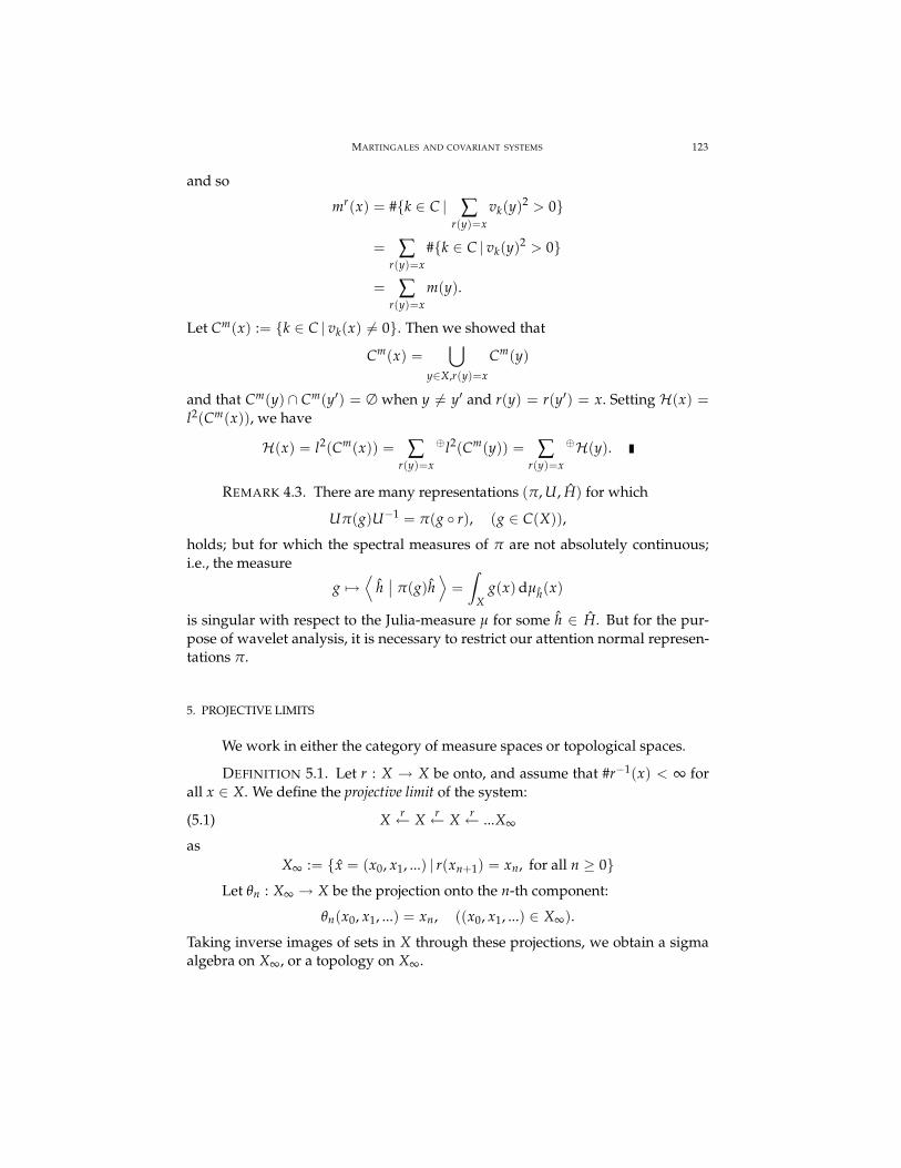
and so

mr(x) = #k ∈ C | ∑r(y)=x

vk(y)2> 0

= ∑r(y)=x

#k ∈ C | vk(y)2> 0

= ∑r(y)=x

m(y).

Let Cm(x) := k ∈ C | vk(x) 6= 0. Then we showed that

Cm(x) =⋃

y∈X,r(y)=x

Cm(y)

and that Cm(y) ∩ Cm(y′) = ∅ when y 6= y′ and r(y) = r(y′) = x. Setting H(x) =

l2(Cm(x)), we have

H(x) = l2(Cm(x)) = ∑r(y)=x

⊕l2(Cm(y)) = ∑r(y)=x

⊕H(y).

REMARK 4.3. There are many representations (π, U, H) for which

Uπ(g)U−1 = π(g r), (g ∈ C(X)),

holds; but for which the spectral measures of π are not absolutely continuous;i.e., the measure

g 7→⟨

h∣

∣ π(g)h⟩

=

∫

Xg(x) dµh(x)

is singular with respect to the Julia-measure µ for some h ∈ H. But for the pur-pose of wavelet analysis, it is necessary to restrict our attention normal represen-tations π.

5. PROJECTIVE LIMITS

We work in either the category of measure spaces or topological spaces.

DEFINITION 5.1. Let r : X → X be onto, and assume that #r−1(x) < ∞ forall x ∈ X. We define the projective limit of the system:

(5.1) Xr← X

r← Xr← ...X∞

asX∞ := x = (x0, x1, ...) | r(xn+1) = xn, for all n ≥ 0

Let θn : X∞ → X be the projection onto the n-th component:

θn(x0, x1, ...) = xn, ((x0, x1, ...) ∈ X∞).

Taking inverse images of sets in X through these projections, we obtain a sigmaalgebra on X∞, or a topology on X∞.

124 DUTKAY AND JORGENSEN

We have an induced mapping r : X∞ → X∞ defined by

(5.2) r(x) = (r(x0), x0, x1, ...), and with inverse r−1(x) = (x1, x2, ...).

so r is an automorphism, i.e., r r−1 = idX∞and r−1 r = idX∞

.Note that

θn r = r θn = θn−1.

-

QQ

QQ

QQ

QQQs ?

X∞ X

X

θn

θn−1r

-

QQ

QQ

QQ

QQQs ?

X∞ X∞

X

r

θn−1θn

-

??-

X∞ X∞

X X.

r

θn

r

θn

Consider a probability measure µ on X that satisfies

(5.3)∫

Xf dµ =

∫

X

1#r−1(x)

∑r(y)=x

f (y) dµ(x).

It is known that such measures µ on X exist for a general class of systemsr : X → X. The measure µ is said to be strongly r-invariant. We have alreadydiscussed some in Section 2 above.

If X = X(A) is the state space of a sub-shift, we saw that µ = µA may beconstructed as an application of Ruelle’s theorem (see Lemma 2.6). If X = Julia(r)is the Julia set of some rational mapping, then it is also known [Bea],[Mil] that astrongly r-invariant measure µ on X = Julia(r) exists.

For m0 ∈ L∞(X), define

(5.4) (Rξ)(x) =1

#r−1(x) ∑r(y)=x

|m0(y)|2ξ(y), (ξ ∈ L1(X)).

The next two theorems (Theorem 5.3-5.4) are key to our dilation theory. Thedilations which we construct take place at three levels as follows:

• Dynamical systems

(X, r, µ) endomorphism → (X∞, r, µ), automorphism .

• Hilbert spaces

L2(X, h dµ)→ (Rm0 h = h) → L2(X∞, µ).

• Operators

Sm0 isometry → U unitary (if m0 is non-singular);

M(g) multiplication operator → M∞(g).

DEFINITION 5.2. A function m0 on a measure space is called singular if m0 =

0 on a set of positive measure.

MARTINGALES AND COVARIANT SYSTEMS 125

In general, the operators Sm0 on H0 = L2(X, h dµ), and U on L2(X∞, µ), maybe given only by abstract Hilbert space axioms; but in our martingale representa-tion, we get the following two concrete formulas:

(Sm0 ξ)(x) = m0(x)ξ(r(x)), (x ∈ X, ξ ∈ H0);

(U f )(x) = m0(x0) f (r(x)), (x ∈ X∞, f ∈ L2(X∞, µ)).

THEOREM 5.3. If h ∈ L1(X), h ≥ 0 and Rh = h, then there exists a uniquemeasure µ on X∞ such that

µ θ−1n = ωn, (n ≥ 0),

where

(5.5) ωn( f ) =

∫

XRn( f h) dµ, ( f ∈ L∞(X)).

Proof. It is enough to check that the measures ωn and ωn+1 are compatible,i.e., we have to check if

ωn+1( f r) = ωn( f ), ( f ∈ L∞(X)).

ButRn+1( f r h) = Rn(R( f r h)) = Rn( f Rh) = Rn( f h).

Note that we can identify functions on X with functions on X∞ by

f (x0, x1...) = f (x0), ( f : X → C).

THEOREM 5.4.

(5.6)d(µ r)

dµ= |m0|2

Proof. Equation (5.6) can be rewritten as∫

X∞

|m0|2 f r dµ =

∫

X∞

f dµ, ( f ∈ L∞(µ)).

By the uniqueness of µ, it is enough to check that∫

X∞

|m0|2(x0)( f θn) r(x) dµ(x) = ωn( f ), ( f ∈ L∞(X)),

or, equivalently (since θn r = rθn and x0 = rn(xn)):

(5.7) ωn(|m0|2 rn f r) = ωn( f ).

We can compute:∫

XRn(|m0|2 rn f r h) dµ =

∫

X|m0|2Rn( f r h) dµ

=

∫

X|m0|2Rn−1( f Rh) dµ =

∫

X|m0|2Rn−1( f h) dµ =

∫

XR(Rn−1( f h)) dµ,

and we used (5.3) for the last equality. This proves (5.7) and the theorem.

126 DUTKAY AND JORGENSEN

THEOREM 5.5. Suppose m0 is non-singular, i.e., it does not vanish on a set of

positive measure. Define U on L2(X∞, µ) by

U f = m0 f r, ( f ∈ L2(X∞, µ)),

π(g) f = g f , (g ∈ L∞(X), f ∈ L2(X∞, µ)),

ϕ = 1.

Then (L2(X∞, µ), U, π, ϕ) is the covariant system associated to m0 and h as in Corollary3.6. Moreover, if Mg f = g f for g ∈ L∞(X∞, µ) and f ∈ L2(X∞, µ), then

UMgU−1 = Mgr.

Proof. Theorem 5.4 shows that U is isometric. Since m0 is non-singular, thesame theorem can be used to deduce that

U∗ f =1

m0 r−1 f r−1

is a well defined inverse for U.The covariance relation follows by a direct computation. Also we obtain

U−nπ(g)Un f = g r−n f , (g ∈ L∞(X), f ∈ L2(X∞, µ)),

which shows that ϕ is cyclic.The other requirements of Corollary 3.6, are easily obtained by computa-

tion.

REMARK 5.6. When m0 is singular U is just an isometry (not onto). How-ever, we still have many of the relations: the covariance relation becomes

Uπ( f ) = π( f r)U, ( f ∈ L∞(X)),

the scaling equation remains true,

(5.8) Uϕ = π(m0)ϕ,

and the correlation function of ϕ is h:

〈 ϕ | π( f )ϕ 〉 =

∫

Xf h dµ, ( f ∈ L∞(X)).

We further note that equation (5.8) is an abstract version of the scaling identityfrom wavelet theory. In Section 1 we recalled the scaling equation in its twoequivalent forms, the additive version (1.1), and its multiplicative version (1.2).The two versions are equivalent via the Fourier transform.

6. MARTINGALES

We give now a different representation of the construction of the covariantsystem associated to m0 and h given in Theorem 5.5.

MARTINGALES AND COVARIANT SYSTEMS 127

LetHn := f ∈ L2(X∞, µ) | f = ξ θn, ξ ∈ L2(X, ωn).

Then Hn form an increasing sequence of closed subspaces which have denseunion.

We can identify the functions in Hn with functions in L2(X, ωn), by

in(ξ) = ξ θn, (ξ ∈ L2(X, ωn)).

The definition of µ makes in an isomorphism between Hn and L2(X, ωn).Define

H := (ξ0, ξ1, ...) | ξn ∈ L2(X, ωn), R(ξn+1h) = ξnh, supn

∫

XRn(|ξn|2h) dµ < ∞,

with the scalar product

〈 (ξ0, ξ1, ...) | (η0, η1, ...) 〉 = limn→∞

∫

XRn(ξnηnh) dµ.

THEOREM 6.1. The map Φ : L2(X∞, µ)→ H defined by

Φ( f ) = (i−1n (Pn f ))n≥0,

where Pn is the projection onto Hn is an isomorphism.

ΦUΦ−1(ξn)n≥0 = (m0 rn ξn+1)n≥0,

Φπ(g)Φ−1(ξn)n≥0 = (g rn ξn)n≥0,

Φϕ = (1, 1, ...).

Proof. Let ξn := i−1n (Pn f ). We check that R(ξn+1h) = ξnh. For this it is

enough to see that the projection of ξn+1 θn+1 onto Hn is (R(ξn+1h)/h) θn. Wecompute the scalar products with g θn ∈ Hn:

〈 ξn+1 θn+1 | g θn 〉 =

∫

X∞

ξn+1 θn+1g r θn+1 dµ =

∫

XRn+1(ξn+1g rh) dµ

=

∫

XRn(g

R(ξn+1h)

hh) dµ =

⟨

R(ξn+1h)

h θn

∣

∣

∣ g θn

⟩

.

Since the union of (Hn) is dense, Pn f converges to f . As each in is isometric,

〈 f | g 〉 = limn→∞

〈 Pn f | Png 〉 = limn→∞

〈Φ( f )n | Φ(g)n 〉L2(X,ωn) = 〈Φ( f ) | Φ(g) 〉 .

Now we check that Φ is onto. Take (ξn)n≥0 ∈ H. Then define

fn := ξn θn = i−1n (ξn).

The previous computation shows that

Pn fn+1 = fn.

Also

supn‖ fn‖2 = sup

n

∫

XRn(|ξn|2h) dµ < ∞.

128 DUTKAY AND JORGENSEN

But then, by a standard Hilbert space argument, fn is a Cauchy sequence whichconverges to some

f = limn→∞

fn = f0 +∞

∑k=0

( fk+1 − fk) ∈ L2(X∞, µ)

with Pn f = fn for all n ≥ 0, and we conclude that Φ( f ) = (ξn)n≥0.The form of ΦUΦ−1 and Φπ(g)Φ−1 can be obtain from the next lemma

(using the fact that PnU f = UPn+1).

LEMMA 6.2. The following diagram is commutative

L2(X, ωn)α−→ L2(X, ωn+1)

↓ in ↓ in+1

Hn −→ Hn+1

where α(ξ) = ξ r.

If ξ θn+k ∈ Hn+k, then

(6.1) Pn(ξ θn+k) =Rk(ξh)

h θn.

(6.2) U∗ f = χm0r−1 6=01

m0 r−1 f r−1, ( f ∈ L2(X∞, µ)).

(6.3) UPn+1U∗ = Pn, (n ≥ 0).

Proof. For ξ ∈ L2(X, ωn), ξ θn = ξ r θn+1 = in+1(α(ξ)), thus the diagramcommutes.

We have to check that, for all η ∈ L2(X, ωn) we have

〈 ξ θn+k | η θn 〉 =

⟨

Rk(ξh)

h θn

∣

∣

∣ η θn

⟩

.

But

〈 ξ θn+k | η θn 〉 =

∫

XRn+k(ξη rk h) dµ =

∫

XRn(

Rk(ξh)

hηh) dµ

=

⟨

Rk(ξh)

h θn

∣

∣

∣η θn

⟩

.

Equation (6.2) can be proved by a direct computation.

MARTINGALES AND COVARIANT SYSTEMS 129

Since (Hn) are dense in L2(X∞, µ), we can check (6.3) on Hn+k. Take ξ θn+k ∈ Hn+k, then

UPn+1U∗(ξ θn+k) = UPn+1

(

χm0r−1 6=01

m0 r−1 ξ θn+k r−1)

= UPn+1

((

χm0r−1 6=0 rn+k+1 1m0 rn+k

ξ

)

θn+k+1

)

= U

Rk(

χm0r−1 6=0 rn+k+1 1m0rn+k ξh

)

h

θn+1

= U

((

χm0r−1 6=0 rn+1 1m0 rn

Rk(ξh)

h

)

θn+1

)

= m0χm0r−1 6=0 r1

m0

Rk(ξh)

h θn

= Pn(ξ θn+k).

As a consequence of Lemma 6.2 we also have:

PROPOSITION 6.3. The identification of functions in L2(X, ωn) with martingales

is given by(6.4)

Φ(in(ξ)) =

(

Rn(ξh)

h, ...,

R(ξh)

h, ξ, ξ r, ξ r2, ...

)

, (ξ ∈ L2(X, ωn), n ≥ 0).

The condition that m0 be non-singular is essential if one wants U to be uni-tary. We illustrate this by an example.

EXAMPLE 6.4 (Shannon’s wavelet). Let R/Z ≃ [− 12 , 1

2 ). By this we meanthat functions on [− 1

2 , 12 ) are viewed also as functions on R via periodic extension,

i.e., f (x + n) = f (x) if x ∈ [− 12 , 1

2 ) and n ∈ Z.Set

m0(x) =√

2χ[− 14 , 1

4 )(x).

Then

(6.5) ϕ(x) =∞

∏k=1

1√2

m0

( x

2k

)

= χ[− 14 , 1

4 )

(x

2

)

= χ[− 12 , 1

2 )(x),

and

ϕ(t) =sin πt

πt.

For functions in L1(R/Z), the Ruelle operator Rm0 is

(Rm0 f )(x) = χ[− 14 , 1

4 )(x

2) f (

x

2) + χ[− 1

4 , 14 )(

x + 12

) f (x + 1

2) = χ[− 1

4 , 14 )(

x

2) f (

x

2)

= χ[− 12 , 1

2 )(x) f (x

2) = f (

x

2), for x ∈ [−1

2,

12).

130 DUTKAY AND JORGENSEN

Hence Rm01 = 1.Note from (6.5) that ϕ(x + n) = 0 if n ∈ Z \ 0.Let ξ ∈ L2(R/Z). Then we get

∫

X∞

|ξ θn|2 dµ =

∫

X|ξ|2 dωn =

∫ 12

− 12

Rn(|ξ|2)(x) dx

=

∫ 12

− 12

|ξ(2−nx)|2 dx = 2n∫ 1

2n+1

− 12n+1

|ξ(x)|2 dx.

But then L2(X, ωn) = L2([− 12n+1 , 1

2n+1 ), 2n dx) and we see that the map

α : L2(X, ωn) → L2(X, ωn+1), α(ξ) = ξ(2·)

is an isometry (Lemma 6.2) which is also surjective with inverse ξ 7→ ξ( x2 ).

With Lemma 6.2, we get that the inclusion of Hn in Hn+1 is in fact an identity,therefore

L2(X∞, µ) = H0 = L2([−12

,12), dx).

When m0 is non-singular, Theorem 5.5 shows that the covariant system(L2(X∞, µ), U, π, ϕ) has U unitary so, by uniqueness, it is isomorphic to the oneconstructed via the Kolmogorov theorem in Corollary 3.6, which we denote by(H, U, π, ϕ).

The next theorem shows that even when m0 is singular, the covariant system(L2(X∞, µ), U, π, ϕ) can be embedded in the (H, U, π, ϕ).

THEOREM 6.5. There exists a unique isometry Ψ : L2(X∞, µ) → H such that

Ψ(ξ θn) = U−nπ(ξ)Un ϕ, (ξ ∈ L∞(X, µ)).

Ψ intertwines the two systems, i.e.,

ΨU = UΨ, Ψπ(g) = π(g)Ψ, for g ∈ L∞(X, µ), Ψϕ = ϕ.

Proof. Let jn : Hn → H be defined on a dense subspace by

jn(ξ θn) = U−nπ(ξ)Un ϕ, (ξ ∈ L∞(X, µ)).

Then jn is a well defined isometry because

‖ξ θn‖2L2(µ)

=

∫

XRn(|ξ|2h) dµ =

∫

X|m(n)

0 |2|ξ|2 dµ = ‖U−nπ(ξ)Un ϕ‖2,

wherem

(n)0 := m0 ·m0 r · .. ·m0 rn−1.

Also note that

jn+1(ξ θn) = jn(ξ r θn+1) = U−n−1π(ξ r)Un+1 ϕ = U−nπ(ξ)Un ϕ,

so we can construct Ψ on L2(X∞, µ) such that it agrees with jn on Hn.

MARTINGALES AND COVARIANT SYSTEMS 131

Next, we check the intertwining properties; it is enough to verify them onHn:

UΨ(ξ θn) = UU−nπ(ξ)Un ϕ = U−n+1π(ξ r)Un−1U ϕ

= U−n+1π(ξ)Un−1π(m0)ϕ,

ΨU(ξ θn) = Ψ(m0ξ θn r) = Ψ((m0 rn−1ξ) θn−1)

= U−n+1π(m0 rn−1ξ)Un−1 ϕ = U−n+1π(ξ)Un−1π(m0)ϕ.

The other intertwining relations can be checked by some similar computations.

6.1. CONDITIONAL EXPECTATIONS. We can consider the σ-algebras

Bn := θ−1n (B),

B being the σ-algebra of Borel subsets in X. Note that θ−1n (E) = θ−1

n+1(r−1(E)). Iffollows that

B0 ⊂ B1 ⊂ ... ⊂ Bn ⊂ Bn+1 ⊂ ...We set B∞ = ∪n≥0Bn which is a sigma-algebra on X∞.

The functions on X∞ which are Bn measurable are the functions which de-pend only on x0, ..., xn. Hn consists of function in L2(X∞, Bn, µ). Also we can re-gard L∞(X∞, Bn, µ) as an increasing sequence of subalgebras of L∞(X∞, µ). Themap

in : L∞(X, ωn) → L∞(X∞, Bn, µ)

is an isomorphism.An application of the Radon-Nikodym theorem shows that there exists a

unique conditional expectation En : L1(X∞, µ) → L1(X∞, Bn, µ) determined by therelation

(6.6)∫

X∞

En( f )g dµ =

∫

X∞

f g dµ, (g ∈ L∞(X∞, Bn, µ)).

We enumerate the properties of these conditional expectations.

PROPOSITION 6.6.

(6.7) En( f g) = f En(g), ( f ∈ L∞(X∞, Bn, µ), g ∈ L1(X∞, µ)),

(6.8) En( f ) ≥ 0, if f ≥ 0,

(6.9) EmEn = EnEm = En, if m ≥ n,

(6.10)∫

X∞

En( f ) dµ =

∫

X∞

f dµ,

(6.11) En( f ) = Pn( f ), if f ∈ L2(X∞, µ).

132 DUTKAY AND JORGENSEN

DEFINITION 6.7. A sequence ( fn)n≥0 of measurable functions on X∞ is saidto be a martingale if

En fn+1 = fn, (n ≥ 0),

where En is a family of conditional expectations as in Proposition 6.6.

PROPOSITION 6.8. If ξ ∈ L1(X, ωn+k) then

(6.12) En(ξ θn+k) =Rk(ξh)

h θn

Proof. If ξ ∈ L2(X, ωn), the formula follows from Lemma 6.2. The rest fol-lows by approximation.

Proposition 6.8 offers a direct link between the operator powers Rk and theconditional expectations En. It shows in particular how our martingale construc-tion depends on the Ruelle operator R. For a sequence (ξn)n≥0 of measurablefunctions on X, (ξn θn)n≥0 is a martingale if and only if

R(ξn+1h) = ξnh, (n ≥ 0).

A direct application of Doob’s theorem (Theorem IV-1-2, in [Neveu]) givesthe following:

PROPOSITION 6.9. If ξn ∈ L1(X, ωn) is a sequence of functions with the propertythat

R(ξn+1h) = ξnh, (n ≥ 0),

then the sequence ξn θn converges µ-almost everywhere.

Then Proposition IV-2-3 from [Neveu], translates into

PROPOSITION 6.10. Suppose ξn ∈ L1(X, ωn) is a sequence with the propertythat

R(ξn+1h) = ξnh, (n ≥ 0).

The following conditions are equivalent:

(i) The sequence ξn θn converges in L1(X∞, µ).(ii) supn

∫

X Rn(|ξ|h) dµ < ∞ and the a.e. limit ξ∞ = limn ξn θn satisfies ξn θn = En(ξ∞).

(iii) There exists a function ξ ∈ L1(X∞, µ) such that ξn θn = En(ξ) for all n.

(iv) The sequence ξn θn satisfies the uniform integrability condition:

supn

∫

XRn(χ|ξn|>aξnh) dµ ↓ 0 as a ↑ ∞

.

If one of the conditions is satisfied, the martingale (ξn)n is called regular.

Convergence in Lp is given by Proposition IV-2-7 in [Neveu]:

MARTINGALES AND COVARIANT SYSTEMS 133

PROPOSITION 6.11. Let p > 1. Every martingale (ξn)n with ξn ∈ Lp(X, ωn)

and

supn‖ξn‖p < ∞

is regular, and ξn θn converges in Lp(X∞, µ) to ξ∞.

We have seen that functions f on X∞ may be identified with sequences (ξn)

of functions on X. When r : X → X is given, the induced mappings

(6.13) r : X∞ → X∞, and r−1 : X∞ → X∞

yield transformations of functions on X∞ as follows f 7→ f r and f 7→ f r−1.The 1-1 correspondence

(6.14) f function on X∞ ↔ ξ0, ξ1, ... functions on X

is determined uniquely by

(6.15) En( f ) = ξn θn, n = 0, 1, ...

When f and h are given, then the functions (ξn) in (6.14) must satisfy

(6.16) R(ξn+1h) = ξnh, (n ≥ 0)

PROPOSITION 6.12. Assume m0 is non-singular. If f is a function on X∞ andf ↔ (ξn) as in (6.14) then

(6.17) f r ↔ ξn+1

(6.18) f r−1 ↔ ξn−1

Specifically we have

(6.19) En( f r) = ξn+1 θn

and

(6.20) En( f r−1) = ξn−1 θn =

(

R(ξnh)

h

)

θn

Or equivalently

(6.21) f r ↔ (ξ1, ξ2, ...),

and

(6.22) f r−1 ↔ (R(ξ0h)

h, ξ0, ξ1, ...).

134 DUTKAY AND JORGENSEN

Proof. Theorem 5.4 is used in both parts of the proof below.We have for g : X → C,

∫

X∞

En( f r) g θn dµ =

∫

X∞

f r g θn+1 r dµ =

∫

X∞

1|m0|2 r−1 f g θn+1 dµ

=

∫

X∞

En+1( f )

(

1|m0|2 rn

g

)

θn+1 dµ

=

∫

X∞

ξn+1 θn r−1(

1|m0|2 rn

g

)

θn r−1 dµ

=

∫

X∞

|m0|2ξn+1 θn1|m0|2

g θn dµ

=

∫

X∞

ξn+1 θn g θn dµ.

Thus En( f r) = ξn+1 θn.

∫

X∞

En( f r−1)gn θn dµ =

∫

X∞

f r−1 gn θn−1 r−1 dµ

=

∫

X∞

|m0|2 f gn θn−1 dµ

=

∫

X∞

En−1( f )(

|m0|2 rn−1 g)

θn−1 dµ

=

∫

X∞

ξn−1 θn r(

|m0|2 rn−1 g)

θn r dµ

=

∫

X∞

1|m0|2 r−1 ξn−1 θn |m0|2 r−1 g θn dµ

=

∫

X∞

ξn−1 θn g θn dµ

and this implies (6.20).

7. INTERTWINING OPERATORS AND COCYCLES

In the paper [DaLa98], Dai and Larson showed that the familiar orthogonalwavelet systems have an attractive representation theoretic formulation. Thisformulation brings out the geometric properties of wavelet analysis especiallynicely, and it led to the discovery of wavelet sets, i.e., singly generated wavelets inL2(Rd), i.e., ψ ∈ L2(Rd) such that ψ = χE for some E ⊂ Rd, and

|detA|j/2ψ(Aj · −k) | j ∈ Z, k ∈ Zd

is an orthonormal basis.

MARTINGALES AND COVARIANT SYSTEMS 135

The case when the initial resolution subspace for some wavelet constructionis singly generated, the wavelet functions should be thought of as wandering vec-tors. If the scaling operation is realized as a unitary operator U in the Hilbert spaceH := L2(Rd), then the notion of wandering, refers to vectors, or subspaces whichare mapped into orthogonal vectors ( respectively, subspaces) under powers ofU. Since this approach yields wavelet bases derived directly from the initial data,i.e., from the wandering vectors, U, and the integral translations, the question ofintertwining operators is a natural one. The initial data defines a representationρ.

An operator in H which intertwines ρ with itself is said to be in the commu-tant of ρ; and Dai and Larson gave a formula for the commutant. They showedthat the operators in the commutant are defined in a natural way from a classof invariant bounded measurable functions, called wavelet multipliers. This andother related results can be shown to generalize to the case of operators whichintertwine two wavelet representations ρ and ρ′.

Since our present martingale construction is a generalization of the tradi-tional wavelet resolutions, see [Jor06], it is natural to ask for theorems whichgeneralize the known theorems about wavelet functions. We prove in this sectionsuch a theorem, Theorem 7.2. The applications of this are manifold, and includethe projective systems defined from Julia sets, and from the state space of a sub-shift in symbolic dynamics.

Our formula for the commutant in this general context of projective systemsis shown to be related to the Perron-Frobenius-Ruelle operator in Corollary 7.3.This result implies in particular that the commutant is abelian; and it makes pre-cise the way in which the representation ρ itself decomposes as a direct integralover the commutant.

Our proof of this corollary depends again on Doob’s martingale conver-gence theorem, see (7.11) below, Section 6 above, and [Jor06], Chapter 2.7.

DEFINITION 7.1. If m0 ∈ L∞(X) and h ∈ L1(X), we call (m0, h) a Perron-Ruelle-Frobenius pair if

Rm0 h = h.

THEOREM 7.2. Let (m0, h) and (m′0, h′) be two Perron-Ruelle-Frobenius pairs

with m0, m′0 non-singular, and let (L2(X∞, µ), U, π, ϕ), (L2(X∞, µ′), U ′, π′, ϕ′) be the

associated covariant systems. Let X∞ = Xa∞ ∪ Xs

∞ be the Jordan decomposition of µ′

with respect to µ, Xa∞ ∩ Xs

∞ = ∅, with µ(Xs∞) = 0 and µ′|Xa

∞≺ µ, and denote by

∆ :=d µ′|Xa

∞

dµ.

Then there is a 1-1 correspondence between each two of the following sets of data:

136 DUTKAY AND JORGENSEN

(i) Operators A : L2(X∞, µ) → L2(X∞, µ′) that intertwine the covariant system,

i.e.,

(7.1) U ′A = AU, and π′(g)A = π(g)A, for g ∈ L∞(X).

(ii) B∞-measurable functions f : X → C such that f |Xs∞

= 0, f ∆12 is µ-bounded

and

(7.2) m0 f = m′0 f r, µ′ − a.e.

(iii) Measurable functions h0 : X → C such that

(7.3) |h0|2 ≤ chh′ µ-a.e.,

for some finite constant c ≥ 0, with

(7.4)1

#r−1(x)∑

r(y)=x

m′0(y)m0(y)h0(y) = h0(x), for µ-a.e. x ∈ X.

From (i) to (ii) the correspondence is given by

(7.5) Aξ = f ξ, (ξ ∈ L2(X∞, µ)).

From (ii) to (iii), the correspondence is given by

(7.6) h0 = Eµ′

0 ( f )h′ = Eµ0 ( f ∆)h

From (i) to (iii) the correspondence is given by

(7.7)⟨

ϕ′ | Aπ(g)ϕ⟩

=

∫

Xgh0 dµ, (g ∈ L∞(X)).

Proof. Take A as in (i). Then for all g ∈ L∞(X) and any n ≥ 0 we have that

A(g r−n) = A(U−nπ(g)Un)(1) = (U ′−nπ′(g)U ′n)(A(1)) = g r−n · (A(1)).

Denote by f := A(1) ∈ L2(X∞, µ′).Since any B∞-measurable, bounded function ξ : X∞ → C can be pointwise

µ− and µ′−approximated by functions of the form g r−n, we get that

A(ξ) = f ξ.

We have also that∫

X∞

| f |2|ξ|2 dµ′ ≤ ‖A‖2∫

X∞

|ξ|2 dµ

so∫

Xa∞

| f |2|ξ|2∆ dµ +

∫

Xs∞

| f |2|ξ|2 dµ′ ≤ ‖A‖2∫

X∞

|ξ|2 dµ

Taking ξ = χXs∞

we obtain that f = 0 µ′-a.e. on Xs∞; so we may take f = 0 on Xs

∞.Then we get also that | f ∆1/2| ≤ ‖A‖ µ-a.e.

Then, again by approximation we obtain that

Aξ = f ξ, for ξ ∈ L2(X∞, µ).

We have in addition the fact that U ′A = AU, and this implies (7.2).

MARTINGALES AND COVARIANT SYSTEMS 137

Conversely, the previous calculations show that any operator defined by(7.5) with f as in (ii), will be a bounded operator which intertwines the covariantsystems.

Now take A as in (i) and consider the linear functional

g ∈ L∞(X) 7→⟨

ϕ′ | Aπ(g)ϕ⟩

This defines a measure on X which is absolutely continuous with respect to µ.Let h0 be its Radon-Nikodym derivative. We have

∫

Xgh0 dµ =

⟨

ϕ′ | Aπ(g)ϕ⟩

=⟨

U ′ϕ′ | U ′Aπ(g)ϕ⟩

=⟨

π′(m′0)ϕ′ | Aπ(g r)π(m0)ϕ⟩

=

∫

Xm′0m0g r h0 dµ

=

∫

Xg

1#r−1(x)

∑r(y)=x

m′0(y)m0(y)h0(y) dµ(x)

Thus 1#r−1(x) ∑r(y)=x m′0(y)m0(y)h0(y) = h0(x) µ-a.e.

Next we check that |h0|2 ≤ ‖A‖2hh′ µ-a.e. By the Schwarz inequality, wehave for all f , g ∈ L∞(X),

|⟨

π′( f )ϕ′ | Aπ(g)ϕ⟩

|2 ≤ ‖A‖2‖π′( f )ϕ′‖2‖π(g)ϕ‖2,

which translates into

(7.8) |∫

Xf gh0 dµ|2 ≤ ‖A‖2

∫

X|g|2h′ dµ

∫

X| f |2h dµ.

If µ has some atoms then just take f and g to be the characteristic function of thatatoms and this proves the inequality (7.3) for such points. The part of µ that doesnot have atoms is measure theoretically isomorphic to the unit interval with theLebesgue measure. Then take x to be a Lebesgue differentiability point for h0, h

and h′. Take f = g = 1µ(I) χI for some small interval centered at x. Letting I shrink

to x and using Lebesgue’s differentiability theorem, (7.8) implies (7.3).For the converse, from (iii) to (i), let h0 as in (iii), and define for n ≥ 0 the

sesquilinear form, Bn on H′n × Hn (see Section 4): for f , g ∈ L∞(X),

Bn(U ′−nπ′( f )ϕ′, U−nπ(g)ϕ) :=∫

Xf gh0 dµ

An application of the Schwarz inequality and (7.3), shows that

|Bn(ξ, η)|2 ≤ c‖ξ‖2‖η‖2, (ξ ∈ H′n, η ∈ Hn).

The inclusion of Hn in Hn+1 is given by

U−nπ( f )ϕ 7→ U−n−1π( f r m0)ϕ.

138 DUTKAY AND JORGENSEN

The forms Bn are compatible with these inclusion in the sense that

Bn+1(U ′−n−1π′( f rm′0)ϕ′, U−n−1π(g rm0)ϕ)

=

∫

Xf rm′0g rm0h0 dµ =

∫

Xf gh0 = Bn(U ′−nπ′( f )ϕ′, U−nπ(g)ϕ)

(We used (7.4) for the third equality.) Therefore the system (Bn)n extends to asesquilinear map B on H′ × H such that its restriction to H′n × Hn is Bn, and Bis bounded (H = L2(X∞, µ), H′ = L2(X∞, µ′).) Then there exists a boundedoperator A : H → H′ such that

〈 ξ | Aη 〉 = B(ξ, η), (ξ ∈ H, η ∈ H′).

We have to check that A is intertwining. But⟨

U ′−nπ′( f )ϕ′∣

∣ AUU−nπ(g)ϕ⟩

= B(U ′−nπ′( f )ϕ′, U−nπ(g r m0)ϕ)

=

∫

Xf g r m0h0 dµ

= B(U ′−n−1π′( f )ϕ′, U−n−1π(g r m0)ϕ)

=⟨

U ′−n−1π′( f )ϕ′∣

∣ AU−n−1π(g r m0)ϕ⟩

=⟨

U ′−nπ′( f )ϕ′∣

∣ U ′AU−nπ(g)ϕ⟩

.

⟨

U ′−nπ′( f )ϕ′∣

∣ Aπ(k)U−nπ(g)ϕ⟩

= B(U ′−nπ′( f )ϕ′, U−nπ(k rn g)ϕ)

=

∫

Xf k rn gh0 dµ

= B(U ′−nπ′(k rn f )ϕ′, U−nπ(g)ϕ)

=⟨

U ′−nπ′(k rn f )ϕ′∣

∣ AU−nπ(g)ϕ⟩

=⟨

π′(k)U ′−nπ′( f )ϕ′∣

∣ AU−nπ(g)ϕ⟩

=⟨

U ′−nπ′( f )ϕ′∣

∣ π′(k)AU−nπ(g)ϕ⟩

.

This shows that A is intertwining.From (ii) to (iii), take f as in (ii). Then define the operator A as in (7.5).

Using the previous correspondences we have that A is intertwining and thereexists h0 as in (iii), satisfying (7.7). We rewrite this in terms of f , and we have forall g ∈ L∞(X):

∫

XE

µ′

0 ( f )gh′ dµ =

∫

X∞

f g dµ′ =⟨

ϕ′ | Aπ(g)ϕ⟩

=

∫

Xgh0 dµ

Also∫

X∞

f g dµ′ =∫

Xa∞

f g∆ dµ =

∫

XE

µ0 ( f ∆)gh dµ.

This proves (7.6).

MARTINGALES AND COVARIANT SYSTEMS 139

COROLLARY 7.3. Let (m0, h) be a Perron-Ruelle-Frobenius pair with m0 non-

singular.

(i) For each operator A on L2(X∞, µ) which commutes with U and π, there exists

a cocycle f , i.e., a bounded measurable function f : X∞ → C with f = f r,µ-a.e., such that

(7.9) A = M f ,

and, conversely each cocycle defines an operator in the commutant.(ii) For each measurable harmonic function h0 : X → C, i.e., Rm0 h0 = h0, with

|h0|2 ≤ ch2 for some c ≥ 0, there exists a unique cocycle f such that

(7.10) h0 = E0( f )h,

and conversely, for each cocycle the function h0 defined by (7.10) is harmonic.(iii) The correspondence h0 → f in (ii) is given by

(7.11) f = limn→∞

h0

h θn

where the limit is pointwise µ-a.e., and in Lp(X∞, µ) for all 1 ≤ p < ∞.

Proof. (i) and (ii) are direct consequences of Theorem 7.2. For (iii), we havethat f ∈ L∞(X∞, µ) ⊂ Lp(X∞, µ). Using Proposition 6.12, we have that, sincef = f r, if En( f ) = ξn θn, then

ξn = ξn+1, for all n ≥ 0.

But from (7.10), we know that ξ0 = h0h , so

En( f ) =h0

h θn.

(iii) follows now from Propositions 6.9, 6.10 and 6.11.

8. ITERATED FUNCTION SYSTEMS

In Section 6 we constructed our extension systems using martingales, andDoob’s convergence theorem. We showed that our family of martingale Hilbertspaces may be realized as L2(X∞, µ), where both X∞, and the associated measuresµ on X∞ are projective limits constructed directly from the following given data.Our construction starts with the following four: (1) a compact metric space X,(2) a given mapping r : X → X, (3) a strongly invariant measure µ on X, and(4) a function W on X which prescribes transition probabilities. From this, weconstruct our extension systems.

In this section, we take a closer look at the measure µ. We show that µ isin fact an average over an indexed family of measures Px, x in X. Now Px isconstructed as a measure on a certain space of paths. The subscript x refers to

140 DUTKAY AND JORGENSEN

the starting point of the paths, and Px is defined on a sigma-algebra of subsets ofpath-space. (The reader is referred to [Jor06] for additional details.)

These are paths of a random walk, and the random walk is closely con-nected to the mathematics of the projective limit construction in Section 4. Butthe individual measures Px carry more information than the averaged version µ

from Section 4. As we show below, the construction of solutions to the canonicalscaling identities in wavelet theory, and in dynamics, depend on the path spacemeasures Px. Our solutions will be infinite products, and the pointwise conver-gence of these infinite products depends directly on the analytic properties of thePx’s.

Let X be a metric space and r : X → X an N to 1 map. Denote by τk : X → X,k ∈ 1, ..., N, the branches of r, i.e., r(τk(x)) = x for x ∈ X, the sets τk(X) aredisjoint and they cover X.

Let µ be a measure on X with the property

(8.1) µ =1N

N

∑k=1

µ τ−1k .

This can be rewritten as

(8.2)∫

Xf (x) dµ(x) =

1N

N

∑k=1

∫

Xf (τk(x)) dµ(x),

which is equivalent also to the strong invariance property.Let W, h ≥ 0 be two functions on X such that

(8.3)N

∑k=1

W(τk(x))h(τk(x)) = h(x), (x ∈ X).

Denote byΩ := ΩN := ∏

N

1, ..., N.

Also we denote by

W(n)(x) := W(x)W(r(x))...W(rn−1(x)), (x ∈ X).

PROPOSITION 8.1. For every x ∈ X there exists a positive Radon measure Px on

Ω such that, if f is a bounded measurable function on Ω which depends only on the firstn coordinates ω1, ..., ωn, then

(8.4)∫

Ωf (ω) dPx(ω)

= ∑ω1,...,ωn

W(n)(τωn τωn−1...τω1(x))h(τωn τωn−1...τω1(x)) f (ω1, ..., ωn).

Proof. We check that Px is well defined on functions which depend onlyon a finite number of coordinates. For this, take f measurable and bounded,depending only on ω1, ..., ωn; and consider it as function which depends on the

MARTINGALES AND COVARIANT SYSTEMS 141

first n + 1 coordinates. We have to check that the two formulas given by (8.4)yield the same result.

Consistency: As a function of the first n + 1 coordinates, we have

∫

Xf (ω) dPx(ω) = ∑

ω1,...,ωn+1

W(n+1)(τωn+1...τω1(x))h(τωn+1...τω1(x)) f (ω1, ..., ωn+1)

= ∑ω1,...,ωn

f (ω1, ..., ωn)W(n)(τωn ...τω1(x))

· ∑ωn+1

W(τωn+1...τω1(x))h(τωn+1...τω1(x))

= ∑ω1,...,ωn

W(n)(τωn ...τω1(x)) f (ω1, ..., ωn)h(τωn ...τω1(x)),

so Px is well defined. Using the Stone-Weierstrass and Riesz theorems, we obtainthe desired measure.

Consider now the space X ×Ω. On this space we have the shift S:

(8.5) S(x, ω1...ωn...) = (r(x), ωxω1...ωn...), (x ∈ X, (ω1...ωn...) ∈ Ω),

where ωx is defined by x ∈ τωx(X). The inverse of the shift is given by theformula:

(8.6) S−1(x, ω1...ωn...) = (τω1(x), ω2...ωn...), (x ∈ X, (ω1...ωn...) ∈ Ω).

PROPOSITION 8.2. Define the map Ψ : X∞ → X ×Ω by

Ψ(x0, x1, ...) = (x0, ω1, ω2, ...), where xn = τωn(xn−1), (n ≥ 1).

Then Ψ is a measurable bijection with inverse

Ψ−1(x, ω1, ω2, ...) = (x, τω1(x), τω2τω1(x), ...).

(8.7) Ψ r Ψ−1 = S.

Also

(8.8)∫

X∞

f dµ =

∫

X

∫

Ωf Ψ−1(x, ω) dPx(ω) dµ(x), ( f ∈ L1(X∞, µ)).

Proof. We know that r(xn) = xn−1 therefore xn = τωn(xn−1) for some ωn ∈1, ..., N. This correspondence defines Ψ and it is clear that the map is 1-1 andonto and the inverse has the given formula. A computation proves (8.7).

142 DUTKAY AND JORGENSEN

To check (8.8), it is enough to verify the conditions of Theorem 5.3. Takeξ ∈ L∞(X), then ξ θn Ψ−1 depends only on x and ω1, ..., ωn so

∫

X

∫

Ωf θn Ψ−1(x, ω) dPx(ω) dµ(x)

=

∫

X∑

ω1,...,ωn

W(n)(τωn τωn−1...τω1(x))

· h(τωn τωn−1...τω1(x))( f θnΨ−1)(x, ω) dµ(x)

=

∫

XRn( f h)(x) dµ(x) =

∫

X∞

f θn dµ.

This proves (8.8).

Acknowledgements. We gratefully acknowledge discussions with the members of thegroup FRG/NSF; especially enlightening suggestions from Professors L. Baggett, D. Lar-son, and G. Olafsson.

In addition, this work was supported at the University of Iowa by a grant fromthe National Science Foundation (NSF-USA) under a Focused Research Program, DMS-0139473 (FRG).

REFERENCES

[Aya04] A. AYACHE, Hausdorff dimension of the graph of the fractional Brownian sheet,Rev. Mat. Iberoamericana 20 (2004), 395–412.

[Aro] N. ARONSZAJN, Theory of reproducing kernels, Trans. Amer. Math. Soc. 68

(1950), 337–404.

[BCMO] L.W. BAGGETT, A. CAREY, W. MORAN, P. OHRING, General existence theoremsfor orthonormal wavelets, an abstract approach, Publ. Res. Inst. Math. Sci. 31

(1995), 95–111.

[BM] L.W. BAGGETT, K.D. MERRILL, Abstract harmonic analysis and wavelets inR

n, The Functional and Harmonic Analysis of Wavelets and Frames (San Antonio,

1999) (L.W. Baggett and D.R. Larson, eds.), Contemp. Math., vol. 247, AmericanMathematical Society, Providence, 1999, pp. 17–27.

[Bal00] V. BALADI, Positive Transfer Operators and Decay of Correlations, World Scientific,River Edge, NJ, Singapore, 2000.

[BCR84] C. BERG, J.P.R. CHRISTENSEN, P. RESSEL, Harmonic Analysis on Semigroups:

Theory of Positive Definite and Related Functions, Grad. Texts in Math., vol. 100,Springer-Verlag, New York, 1984.

[Bea] A.F. BEARDON, Iteration of Rational Functions: Complex Analytic Dynamical Sys-

tems, Grad. Texts in Math., vol. 132, Springer-Verlag, New York, 1991.

MARTINGALES AND COVARIANT SYSTEMS 143

[BJMP05] L.W. BAGGETT, P.E.T. JORGENSEN, K. MERILL, J.A. PACKER, Constructionof Parseval wavelets from redundant filter systems, J. Math. Phys. 46 (2005),083502.

[BMP00] D.P. BLECHER, P.S. MUHLY, V.I. PAULSEN, Categories of Operator Modules(Morita Equivalence and Projective Modules), Mem. Amer. Math. Soc. 143 (2000),no. 681.

[Bre96] B. BRENKEN, The local product structure of expansive automorphisms ofsolenoids and their associated C∗-algebras, Canad. J. Math. 48 (1996), 692–709.

[BrJo91] B. BRENKEN, P.E.T. JORGENSEN, A family of dilation crossed product algebras,J. Operator Theory 25 (1991), 299–308.

[BrTo05] H. BRUIN, M. TODD, Markov extensions and lifting measures for complex poly-nomials, preprint, http://arxiv.org/abs/math.DS/0507543.

[DaLa98] X. DAI, D.R. LARSON, Wandering vectors for unitary systems and orthogonalwavelets, Mem. Amer. Math. Soc. 134 (1998), no. 640.

[Dau92] I. DAUBECHIES, Ten Lectures on Wavelets, CBMS-NSF Regional Conf. Ser. inAppl. Math., vol. 61, SIAM, Philadelphia, 1992.

[Doob1] J.L. DOOB, The Brownian movement and stochastic equations, Ann. of Math. (2)

43 (1942), 351–369.

[Doob2] J.L. DOOB, What is a martingale?, Amer. Math. Monthly 78 (1971), 451–463.

[Doob3] J.L. DOOB, Classical Potential Theory and Its Probabilistic Counterpart, Classics inMathematics, Springer-Verlag, Berlin, 2001, reprint of the 1984 ed.

[Dut3] D. DUTKAY, Positive definite maps, representations and frames, Rev. Math.

Phys. 16 (2004), no. 4, 451–477.

[DutJo] D. DUTKAY, P.E.T. JORGENSEN, Wavelets on fractals, to appear in Revista

Matemática Iberoamericana.

[FO00] R. FABEC, G. ÓLAFSSON, A. SENGUPTA, Fock spaces corresponding to positivedefinite linear transformations, to appear in Math. Scand.

[Gun66] R.F. GUNDY, Martingale theory and pointwise convergence of certain orthogo-nal series, Trans. Amer. Math. Soc. 124 (1966), 228–248.

[Gun99] R.F. GUNDY, Two remarks concerning wavelets: Cohen’s criterion for low-passfilters and Meyer’s theorem on linear independence, The Functional and Har-

monic Analysis of Wavelets and Frames (San Antonio, 1999) (L.W. Baggett and D.R.Larson, eds.), Contemp. Math., vol. 247, American Mathematical Society, Prov-idence, 1999, pp. 249–258.

[Gun00] R.F. GUNDY, Low-pass filters, martingales, and multiresolution analyses, Appl.

Comput. Harmon. Anal. 9 (2000), 204–219.

[Gun04] R.F. GUNDY, Wavelets and probability, preprint, Rutgers Univer-sity, material presented during the author’s lecture at the work-shop “Wavelets and Applications”, Barcelona, Spain, July 1–6, 2002,http://www.imub.ub.es/wavelets/Gundy.pdf.

[JMR01] S. JAFFARD, Y. MEYER, R.D. RYAN, Wavelets: Tools for Science & Technology, re-vised edition, SIAM, Philadelphia, 2001.

144 DUTKAY AND JORGENSEN

[Jor01] P.E.T. JORGENSEN, Ruelle Operators: Functions Which Are Harmonic with Re-spect to a Transfer Operator, Mem. Amer. Math. Soc. 152 (2001), no. 720.

[Jor06] P.E.T. JORGENSEN, Analysis and Probability: Wavelets, Signals, Fractals, Grad.Texts in Math., vol. 234, Springer-Verlag, New York, to appear 2006.

[JoMu80] P.E.T. JORGENSEN, P.S. MUHLY, Selfadjoint extensions satisfying the Weyl op-erator commutation relations, J. Analyse Math. 37 (1980), 46–99.

[LaPh76] P.D. LAX, R.S. PHILLIPS, Scattering Theory for Automorphic Functions, Ann. ofMath. Stud., no. 87, Princeton University Press, Princeton, NJ, 1976.

[Mil] J. MILNOR, Dynamics in One Complex Variable, Friedr. Vieweg & Sohn, Braun-schweig, Wiesbaden, 1999.

[Moh03] A. MOHARI, Ergodicity of homogeneous Brownian flows, Stochastic Process.

Appl. 105 (2003), 99–116.

[MoPa92] A. MOHARI, K.R. PARTHASARATHY, On a class of generalised Evans-Hudsonflows related to classical Markov processes, Quantum Probability & Related Topics,

QP VII, World Scientific, River Edge, NJ, 1992, pp. 221–249.

[N] E. NELSON, Topics in Dynamics, I: Flows, Math. Notes, Princeton UniversityPress, Princeton, NJ, 1969.

[Neveu] J. NEVEU, Discrete-Parameter Martingales, revised ed., North-Holland Math. Li-brary, vol. 10, North-Holland, Amsterdam, 1975.

[PaSc72] K.R. PARTHASARATHY, K. SCHMIDT, Positive Definite Kernels, Continuous Tensor

Products, and Central Limit Theorems of Probability Theory, Lecture Notes in Math.,vol. 272, Springer-Verlag, Berlin-New York, 1972.

[Rue89] D. RUELLE, The thermodynamic formalism for expanding maps, Comm. Math.

Phys. 125 (1989), 239–262.

[Rue04] D. RUELLE, Thermodynamic Formalism: The Mathematical Structures of Equilibrium

Statistical Mechanics, second ed., Cambridge Math. Lib., Cambridge UniversityPress, Cambridge, 2004.

[San59] G. SANSONE, Orthogonal Functions, English ed., translated from the Italian byA. H. Diamond, with a foreword by E. Hille, Pure Appl. Math. (N.Y.), vol. IX,Interscience, New York, London, 1959.

[Sti55] W.F. STINESPRING, Positive functions on C∗-algebras, Proc. Amer. Math. Soc. 6

(1955), 211–216.

DORIN ERVIN DUTKAY, DEPARTMENT OF MATHEMATICS, HILL CENTER-BUSCH

CAMPUS, RUTGERS, THE STATE UNIVERSITY OF NEW JERSEY, PISCATAWAY, NJ 08854-8019, U.S.A.

E-mail address: ddutkay@math.rutgers.edu

PALLE E.T. JORGENSEN, DEPARTMENT OF MATHEMATICS, THE UNIVERSITY OF

IOWA, IOWA CITY, IA 52242-1419, U.S.A.E-mail address: jorgen@math.uiowa.edu

Received November dd, 2005.