WHAT’S SO SPECIAL ABOUT EUCLIDEAN DISTANCE?

A CHARACTERIZATION WITH APPLICATIONS TOMOBILITY AND SPATIAL VOTING

MARCELLO D’AGOSTINO AND VALENTINO DARDANONI

Abstract. In this paper we provide an application-oriented characterization of aclass of distance functions monotonically related to the Euclidean distance in termsof some general properties of distance functions between real-valued vectors. Ouranalysis hinges upon two fundamental properties of distance functions that we call“value-sensitivity” and “order-sensitivity”. We show how these two general prop-erties, combined with natural monotonicity considerations, lead to characterizationresults that single out several versions of Euclidean distance from the wide class ofseparable distance functions. We then discuss and motivate our results in two differ-ent and apparently unrelated application areas — mobility measurement and spatialvoting theory — and propose our characterization as a test for deciding whetherEuclidean distance (or some suitable variant) should be used in your favourite appli-cation context.

JEL Classification Numbers: C0, C53, D63, D72.

Keywords: Euclidean Distance, Mobility Measurement, Spatial Voting.

This is the pre-print authors’ version of the paper: M. D’Agostino, V. Dardanoni. What’sso special about Euclidean distance? A characterization with applications to mobility andspatial voting. Social Choice and Welfare 33(2009):211–233.

1. Introduction

The problem of measuring the distance1 between real-valued vectors arises in manyareas of scientific research. In particular, variants of the familiar Euclidean distanceplay a prominent role in many important application contexts not only in economicsand political science, but in such diverse fields as statistics, decision theory, psychology,

Date: 8 October 2008.We would like to thank an Editor and expecially two very perspective referees for useful comments

which helped us to improve the paper substantially.1Our use of the expression “distance”, throughout the paper, is informal. In several application

contexts a variety of functions which do not fully satisfy the standard textbook definition have beentaken into consideration and are regarded as intuitively measuring some sort of distance. So, in thispaper we are not committing to any specific definition, let alone to the standard one. By “distancefunction” we shall refer to any continuous function of two real-valued vectors (of the same finite size)which can be intuitively considered as measuring their distance, even if in some cases, such a functionmay not satisfy some of the properties of the standard definition.

1

2 MARCELLO D’AGOSTINO AND VALENTINO DARDANONI

DNA sequencing, image recognition, weather forecasting and so on.2 But what’s sospecial about Euclidean distance? How can we judge the appropriateness of adoptingthis conventional distance in some specific application context? In what contexts arewe forced to use it (or some monotonic transformation of it) as the appropriate distancefunction?

In this paper we provide an application-oriented characterization of a class of func-tions monotonically related to the Euclidean distance in terms of five general propertieswhich are intuitively (and perhaps empirically) testable. We show that Euclidean dis-tance is (up to a monotonic transformation) the only function that satisfies them all.We also show that, by replacing some of these five properties with suitable variants,one obtains similar characterizations of an averaged version of the Euclidean distancewhich we call Averaged Euclidean Distance, and of closely related distance functionsthat we call Generalized Euclidean Distance and Averaged Generalized Euclidean Dis-tance:

dn(x,y) =√∑n

i=1(xi − yi)2 (ED)

dn(x,y) =√

1n

∑ni=1(xi − yi)2 (AED)

dn(x,y) =√∑n

i=1(g(xi)− g(yi))2 (GED)

dn(x,y) =√

1n

∑ni=1(g(xi)− g(yi))2 (AGED)

where g is a continuous and increasing function. Our results may then be helpful intesting — intuitively or empirically — whether one or the other of these functions fitsa specific application and should, therefore, be preferred to alternative ones.

In this paper we shall speak of a distance function over Xn to mean simply a con-tinuous function dn : Xn × Xn → R+ for some suitable interval X ⊆ R. Since weare interested in evaluating the distance between any two vectors of equal size n, forarbitrary n, our aim is in fact that of investigating infinite classes of distance func-tions over Xn, seeking for some uniform characterization of all their elements. LetX =

⋃∞n=1X

n ×Xn. Then, by a distance over X we mean a infinite collection {dn} ofdistance functions over Xn.

2To mention just a few applications in these fields, Euclidean distance (or some monotonic transfor-mation such as the mean squared error) is often used as a loss function in statistics and decision theory;in psychology, related measures are often employed to evaluate the amount of “similarity” betweentwo objects, each of which is decomposed into a fixed number of components, and (dis)similarityis then modelled as a suitable metric in the resulting feature space ([SJ99]); in biology, there arealgorithms for searching genetic databases for biologically significant similarities in DNA sequencesusing Euclidean and similar distances ([WBD97] and [TJaLA01]); similarity of images (used, amongother things, in security applications) is typically established by appropriate variations of Euclideandistance [WZF05]); accuracy of weather forecasting is traditionally established by the so-called Brierscore ([Bri50]), which is (squared) Euclidean distance between a probability assignment to a sequenceof binary events and the observed outcomes (1 if the event occurs, and 0 if it does not occur).

WHAT’S SO SPECIAL ABOUT EUCLIDEAN DISTANCE 3

6

�

�

�

�

�

�

r

rr

x

y

σ12(y)

-0.4 1

0.2

1

0.7

0.7

(a) Order-sensitive

6

r rr

x

y

y′

-0.4 0.9

0.2

0.4

0.8

(b) Value-sensitive

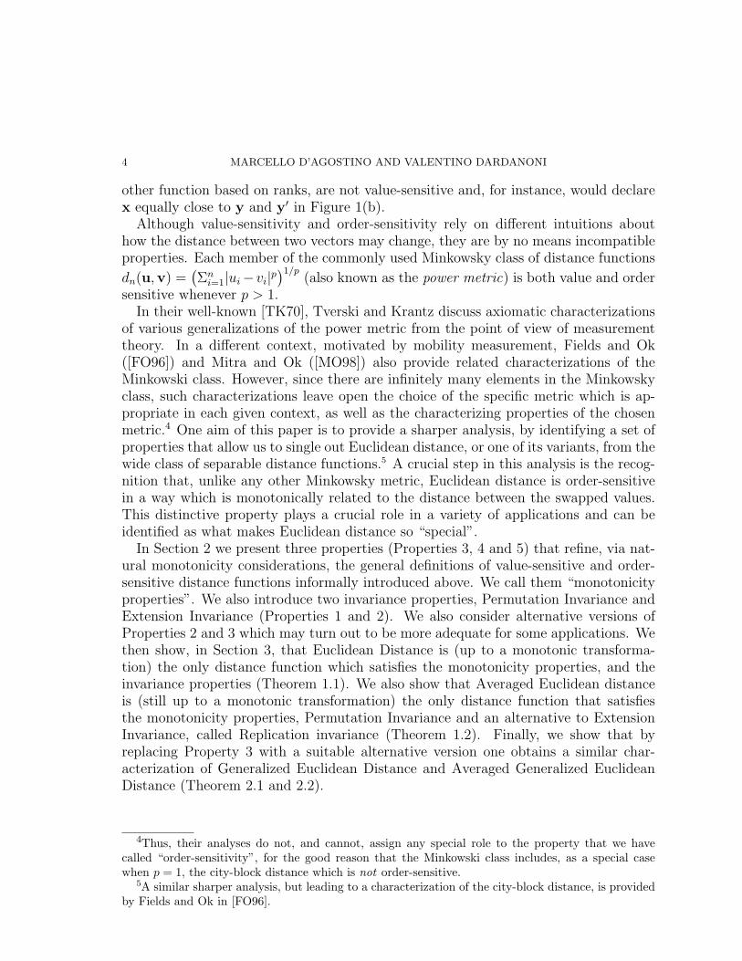
Figure 1. Order-sensitive and value-sensitive functions

Our characterization hinges upon two fundamental properties that a distance func-tion between two real-valued vectors may satisfy. These properties deal with two basicways in which the distance between vectors x and y may intuitively increase/decrease,namely: (a) by altering the distance in one coordinate, leaving everything else un-changed; (b) by “swapping” the values of two coordinates in one of the two vectors,leaving everything else unchanged.

More precisely,

• we say that a distance function dn : Xn×Xn → R+ (for some interval X ⊆ R)is value-sensitive if, for any x,y,y′ ∈ Xn such that d1(xj, yj) < d1(xj, y

′j) and

yi = y′i for i 6= j, we have dn(x,y) < dn(x,y′);• let σij(u) denote the vector obtained from u by “swapping” the values of ui

and uj; a distance function dn is called order-sensitive if, for all x,y ∈ Xn,whenever (xi − xj)(yi − yj) > 0 we have dn(x,y) < dn(x, σij(y)).

While value-sensitivity requires that the distance between two vectors should be amonotonic function of the distance between the values of their corresponding coordi-nates, order-sensitivity requires that it should depend on the order association betweenthe two vectors. Suppose that, for some i and j, there is a positive order associationbetween the corresponding coordinates, that is (xi − xj)(yi − yj) > 0. In this case aswap between yi and yj (or between xi and xj) is order-reversing, since it turns thepositive association into a negative one.3 Order-sensitivity requires that such swapsalways increase the distance between the vectors under consideration.

Clearly, not all commonly used distance functions are order-sensitive. In Figure 1(a)on p. 3, it can be immediately verified that the so-called city-block distance dn(u,v) =Σni=1|ui − vi| declares x as equally close to y and σ12(y). On the other hand, typical

order-sensitive functions, such as the Spearman and Kendall coefficients as well as any

3Such order-reversing swaps are discussed in mathematical statistics [Tch80], economics [ET80],and mobility measurement [Atk83, Dar93].

4 MARCELLO D’AGOSTINO AND VALENTINO DARDANONI

other function based on ranks, are not value-sensitive and, for instance, would declarex equally close to y and y′ in Figure 1(b).

Although value-sensitivity and order-sensitivity rely on different intuitions abouthow the distance between two vectors may change, they are by no means incompatibleproperties. Each member of the commonly used Minkowsky class of distance functions

dn(u,v) =(Σni=1|ui−vi|p

)1/p(also known as the power metric) is both value and order

sensitive whenever p > 1.In their well-known [TK70], Tverski and Krantz discuss axiomatic characterizations

of various generalizations of the power metric from the point of view of measurementtheory. In a different context, motivated by mobility measurement, Fields and Ok([FO96]) and Mitra and Ok ([MO98]) also provide related characterizations of theMinkowski class. However, since there are infinitely many elements in the Minkowskyclass, such characterizations leave open the choice of the specific metric which is ap-propriate in each given context, as well as the characterizing properties of the chosenmetric.4 One aim of this paper is to provide a sharper analysis, by identifying a set ofproperties that allow us to single out Euclidean distance, or one of its variants, from thewide class of separable distance functions.5 A crucial step in this analysis is the recog-nition that, unlike any other Minkowsky metric, Euclidean distance is order-sensitivein a way which is monotonically related to the distance between the swapped values.This distinctive property plays a crucial role in a variety of applications and can beidentified as what makes Euclidean distance so “special”.

In Section 2 we present three properties (Properties 3, 4 and 5) that refine, via nat-ural monotonicity considerations, the general definitions of value-sensitive and order-sensitive distance functions informally introduced above. We call them “monotonicityproperties”. We also introduce two invariance properties, Permutation Invariance andExtension Invariance (Properties 1 and 2). We also consider alternative versions ofProperties 2 and 3 which may turn out to be more adequate for some applications. Wethen show, in Section 3, that Euclidean Distance is (up to a monotonic transforma-tion) the only distance function which satisfies the monotonicity properties, and theinvariance properties (Theorem 1.1). We also show that Averaged Euclidean distanceis (still up to a monotonic transformation) the only distance function that satisfiesthe monotonicity properties, Permutation Invariance and an alternative to ExtensionInvariance, called Replication invariance (Theorem 1.2). Finally, we show that byreplacing Property 3 with a suitable alternative version one obtains a similar char-acterization of Generalized Euclidean Distance and Averaged Generalized EuclideanDistance (Theorem 2.1 and 2.2).

4Thus, their analyses do not, and cannot, assign any special role to the property that we havecalled “order-sensitivity”, for the good reason that the Minkowski class includes, as a special casewhen p = 1, the city-block distance which is not order-sensitive.

5A similar sharper analysis, but leading to a characterization of the city-block distance, is providedby Fields and Ok in [FO96].

WHAT’S SO SPECIAL ABOUT EUCLIDEAN DISTANCE 5

As a vehicle to appreciate the applicative potential of our results, we shall discuss, inSection 4, two case-studies from very different areas: social mobility measurement andspatial voting theory.6 In case-study 1, we make a critical analysis of the characterizingproperties of Euclidean Distance in the context of mobility measurement, which leadsto the rejection of two of these properties on intuitive grounds. Our analysis suggeststhat Averaged Generalized Euclidean Distance may be more suitable for this kind ofapplication. In case-study 2, the intuitive rejection of two characterizing properties ofEuclidean Distance in the context of spatial voting theory is addressed via a differentapproach. This consists in showing how the intuitively judged distance between can-didates, which is prima facie incompatible with a Euclidean metric, can be expressedin terms of a restricted “canonical” model for which all the characterizing propertiesof Euclidean Distance are satisfied.

Potential applications of the characterization results presented in this paper, on theother hand, are by no means restricted to the ones discussed in these two case-studies,but extend to many other interesting problems that can be naturally interpreted interms of choosing a suitable distance function between real-valued vectors.7

2. Properties

As mentioned in the Introduction, we shall speak of a distance function over Xn

to mean simply a continuous function dn : Xn ×Xn → R+ for some suitable intervalX ⊆ R. Moreover, a distance over X =

⋃∞n=1X

n × Xn will be an infinite collection{dn} of distance functions over Xn.

As for the interval X, we shall restrict our attention to three typical cases: (i)X = [0, 1] (ii) X = R+; (iii) X = R. Furthermore, by X+ we mean the nonnegativepart of X, so that X+ is equal to X in cases (i) and (ii), while X+ = R+ in case (iii).Notice that in all cases, given any two x, y ∈ X, their absolute difference |x− y| ∈ X+;this restriction will simplify the analysis and the notation used in this paper.

In what follows we shall use the light-face letters a, b, c, d, etc. to denote arbitraryreal numbers and the boldface letters x,y,w, etc. to denote arbitrary vectors. Thevector whose only element is the real number a will be denoted simply by “a”. Weshall write [x,y] for the concatenation of the two vectors x and y.8

6For surveys on social mobility measurement see Maasoumi [Maa98] and Fields and Ok [FO99a].For an introduction to the spatial theory of voting, see Hinich and Munger [HM70]; for a general moreadvanced treatment of voting theory, Austeen-Smith and Banks [ASB99].

7The linear regression model, for instance, is without doubts the workhorse of theoretical andapplied econometrics. Given an n-sized vector y (“regressand”) and k n-sized vectors x1, . . . ,xk

(“regressors”) which are collected into an n × k design matrix X, the linear regression model dealswith how to find the point in the linear space spanned by the columns of X which is closest to y.Thus, the problem is to find a k-sized vector β (“regression coefficient”) which minimizes the distancebetween y and Xβ. The most common method for solving this problem is of course the OLS, whichimplies that Euclidean distance is the chosen distance concept.

8Since, conventionally, vectors in Xn are columns, by [x,y] we formally mean [xT ,yT ]T .

6 MARCELLO D’AGOSTINO AND VALENTINO DARDANONI

2.1. Invariance Properties. The first property of this group requires each dn to beinvariant under uniform permutations of both its arguments:

Property 1 (Permutation Invariance). For all x,y ∈ Xn and all n ∈ N, dn(x,y) =dn(π(x), π(y)) for every permutation π.

The second property relates the distance between two n-dimensional vectors to thedistance between higher-dimensional “conservative extensions”. It requires that, ifboth vectors are extended by concatenating each of them with the same vector, theirdistance is left unaltered.

Property 2 (Extension Invariance). For all m,n ∈ N, all x,y ∈ Xm and all z ∈ Xn,dm(x,y) = dm+n([x, z], [y, z]).

This Property may appear intuitively sound in some application contexts but not inothers, for instance when we are interested in a notion of averaged distance. For analternative property which is appropriate in such contexts see Section 2.3 below.

2.2. Monotonicity Properties. The first two properties of this group articulate thevalue-sensitivity property informally discussed in Section 1 and refine it via monotonic-ity considerations. They are both rather natural assumptions to make, and similarproperties arise in several characterization results, including those mentioned in theintroduction, in a variety of fields.

Property 3 (One-dimensional value-sensitivity). For all a, b ∈ X, d1(a, b) = G(|a−b|)for some continuous and strictly increasing function G : X+ → R+ such that G(0) = 0.

This property makes one-dimensional distance depend monotonically on the absolutedifference between the values of their single coordinate (G(0) = 0 is a harmless normal-ization requirement) and leaves entirely open the problem of how to measure higher-dimensional distance. Property 3 is closely related to the one called “intradimensionalsubtractivity” in [TK70]. In fact, the latter corresponds to Property 3∗ presented inSection 2.3.

The second property requires that the distance between two vectors is monotonicallyconsistent with the distance between their subvectors:

Property 4 (Subvector Consistency). For all k, j ∈ N and whenever x,y,x′,y′ ∈ Xk,u,v,u′,v′ ∈ Xj,

dk(x,y) > dk(x′,y′) and dj(u,v) = dj(u

′,v′) =⇒=⇒ dk+j([x,u], [y,v]) > dk+j([x

′,u′], [y′,v′]).

A similar axiom is commonly used in the literature on income inequality [Sho88],poverty [FS91] and mobility measurement [FO99b], and implies (as shown in the proofof Theorems 1 and 2 provided in the Appendix, see also [FS91]) the fundamentalindependence assumption which plays a crucial role in the theory of additive conjointmeasurement ([Deb60]). Tverski and Krantz show how to derive the latter from threemore primitive axioms (see Theorem 1 in [TK70]).

WHAT’S SO SPECIAL ABOUT EUCLIDEAN DISTANCE 7

The third property of this group is best understood in connection with the order-sensitivity property discussed in Section 1. It can be interpreted as requiring that theincrease in the distance between two vectors caused by any “order-reversing swap”depends monotonically on the distance, in each vector, between the components thatare involved in the swap:9

Property 5 (Monotonic Order-Sensitivity). For all n ∈ N such that n ≥ 4, for allx,y ∈ Xn and all i, j, k,m ∈ {1, . . . , n}, if

• (xi − xj)(yi − yj) > 0• (xk − xm)(yk − ym) > 0• d1(xi, xj) = d1(xk, xm) and d1(yi, yj) ≤ d1(yk, ym),

then

dn(x, σij(y)) ≤ dn(x, σmk(y)).

In other words, the effect of an order-reversing swap in the y’s depends monotonicallyon the distance between the swapped y’s, provided that the distance between thecorresponding x’s is the same.10 For instance, suppose x = [0, 0.2, 0.4, 0.6] and y =[0, 0.3, 0.5, 1]. The distance between x and σ12(y) = [0.3, 0, 0.5, 1] is smaller than thedistance between x and σ34(y) = [0, 0.3, 1, 0.5], since the distance between the swappedy’s in σ12(y) is smaller than the distance between the swapped y’s in σ34(y) (while thedistance between the corresponding x’s is the same). As will be shown in the nextsection, this property provides a sharp means to single out Euclidean distance (orsome suitable variant of its) from the much wider class of separable distance functions.Observe that, strictly speaking, this Property does not imply, by itself, that the distancefunction be order-sensitive in the sense explained in the Introduction, that is, it doesnot imply that any order-reversing swap be distance-increasing. However, it does so inconjunction with the other properties.11

2.3. Variants. As will be shown in Section 4, Extension Invariance (Property 2 above)may be considered inappropriate in some application contexts — such as social mobilitycomparisons — where we are interested in a notion of average distance. In this kind of

9Recall that we denote by σij(y) the vector obtained from y by “swapping” yi and yj , i.e. thevector y′ such that: (i) y′k = yk for all k 6= i, j, (ii) y′i = yj , and (iii) y′j = yi.

10The latter requirement is necessary for consistency. To see this, observe that the pair of vectors(x, σij(y)) could be seen as obtained from the pair (σij(x), σij(y)) by an order-reversing swap inσij(x). Taking into consideration that Property 5, together with the other properties, implies thatevery order-reversing swap is strictly distance-increasing (see footnote 11 below), it is not difficult toshow that, without this requirement, the property would lead to inconsistent judgements wheneverd1(yi, yj) < d1(yk, ym) and d1(xi, xj) > d1(xk, xm).

11 Let y′ be the vector obtained from y by “swapping” yi and yj , i.e. (i) y′k = yk for all k 6= i, j,(ii) y′i = yj , and (iii) y′j = yi, and assume xj = xi + ∆x and yj = yi + ∆y, with ∆x and ∆y

having the same sign. After the swap, given Theorem 1 below, distance will increase whenever(xi− yi−∆y)2 + (xi + ∆x− yi)2 > (xi− yi)2 + (xi + ∆x− yi−∆y)2; simplifying, the above inequalityholds true, since ∆x∆y is positive.

8 MARCELLO D’AGOSTINO AND VALENTINO DARDANONI

applications one may want to consider, instead of Property 2, a standard “replication”property:

Property 2∗ (Replication Invariance). For every x,y ∈ Xk and every k, n ∈ N,

dk(x,y) = dnk([

n︷ ︸︸ ︷x, · · · ,x], [

n︷ ︸︸ ︷y, · · · ,y]),

where [

n︷ ︸︸ ︷u, · · · ,u] denotes the result of concatenating the vector u with itself n times.

Moreover, One-dimensional Value-Sensitivity (Property 3 above) may also be re-jected, on intuitive or empirical grounds, in favour of the following more general vari-ant:

Property 3∗ (Generalized value-sensitivity). For all a, b ∈ X, d1(a, b) = G(|g(a) −g(b)|) for some continuous and strictly increasing function G : X+ → R+ such thatG(0) = 0, and some continuous and strictly increasing function g : X → X,

where the nature of the function g depends on the application. In Section 4.1, for in-stance, we argue that this variant should be preferred in the context of social mobilitymeasurement, where g can be interpreted as an “economic status” function. [TK70]discuss it in connection with psychological applications and also present (Theorem 1)a different derivation from assumptions expressed in terms of a “betweennes” relation.Observe also that, if Property 3 is replaced by Property 3∗, Property 5 needs to be rein-terpreted by noticing that the distance between the swapped values must be measuredtaking into account the function g.12

3. Characterizations

In what follows, when we say that a distance {dn} over X — intended as an infinitecollection of distance functions over Xn — satisfies a certain property, we mean thatevery element dn of the collection satisfies that property.

Theorem 1. A distance {dn} over X

(1) satisfies Properties 1, 2, 3, 4, 5, if and only if for all n ∈ N and all x,y ∈ Xn:

dn(x,y) = H( n∑i=1

(xi − yi)2),

for some continuous and strictly increasing H : R+ → R+ with H(0) = 0;(2) satisfies Properties 1, 2∗, 3, 4, 5, if and only if for all n ∈ N and all x,y ∈ Xn,

dn(x,y) = H( 1

n

n∑i=1

(xi − yi)2),

for some continuous and strictly increasing H : X+ → R+ with H(0) = 0.

12In particular, when Property 5 is used in conjunction with Property 3∗, one has to recall thatthe third condition of Property 5 becomes |g(xi) − g(xj)| = |g(xk) − g(xm)| and |g(yi) − g(yj)| ≤|g(yk)− g(ym)|), and thus the interpretation of the property depends on g.

WHAT’S SO SPECIAL ABOUT EUCLIDEAN DISTANCE 9

Theorem 2. A distance {dn} over X

(1) satisfies Properties 1, 2, 3∗, 4, 5, if and only if for all n ∈ N and all x,y ∈ Xn,

dn(x,y) = H( n∑i=1

(g(xi)− g(yi))2),

for some continuous and strictly increasing H : R+ → R+ with H(0) = 0;(2) satisfies Properties 1, 2∗, 3∗, 4, 5, if and only if for all n ∈ N and all x,y ∈ Xn,

dn(x,y) = H( 1

n

n∑i=1

(g(xi)− g(yi))2),

for some continuous and strictly increasing H : X+ → R+ with H(0) = 0.

The proof of these theorems is contained in the Appendix.Theorems 1 and 2 can be directly applied to justify the use of one or the other version

of Euclidean distance, in all application contexts in which the relevant properties aresatisfied. Typically, an application context C is represented by some data space andsome intended intuitive distance function over it, i.e. some distance function partiallyspecified by a set of intuitive comparative judgments of the form “x is closer to ythan z”. The problem is determining the functional form that d must have in order tocomply with such intuitive judgments. If the characterizing properties are satisfied bythe intuitive judgments which can be obtained in the application context C – and maysometimes be revealed experimentally – then Theorems 1 and 2 dictate, up to a mono-tonic transformation, the functional form of the distance function: Euclidean Distance(Theorem 1.1), Averaged Euclidean Distance (Theorem 1.2), Generalized EuclideanDistance (Theorem 2.1) and Averaged Generalized Euclidean Distance (Theorem 2.2).

Since these results provide ordinal representations, they clearly do not allow us tosay anything about the specific monotonic transformation that should be adopted ineach particular application context, in particular they do not allow us to discriminatebetween each variant of Euclidean distance and its squared form.13 The choice of theappropriate transformation will depend on further considerations which are application-dependent. We shall end this section by showing, by way of example, how Theorem 1can be strengthened to provide sharper characterizations of ED and AED. For thispurpose consider the following extra property, that we call linear homogeneity :

(Linear Homogeneity). For all n ∈ N, all x,y ∈ Xn and all constants α ∈ X,

dn(αx, αy) = α · dn(x,y).

Then, we can easily obtain the following:

Corollary 1. A distance {dn} over X

13Some monotonic transformations do not give rise, strictly speaking, to a distance function. Forinstance, squared Euclidean Distance does not satisfy the triangle inequality. However, as alreadyexplained in the introduction, in this paper we use the expression “distance function” in a looser way.

10 MARCELLO D’AGOSTINO AND VALENTINO DARDANONI

(1) satisfies Properties 1, 2, 3, 4, 5 and linear homogeneity if and only if for alln ∈ N and all x,y ∈ Xn:

dn(x,y) = β ·

√√√√ n∑i=1

(xi − yi)2,

for some constant β > 0.(2) satisfies Properties 1, 2∗, 3, 4, 5 and linear homogeneity if and only if for all

n ∈ N and all x,y ∈ Xn,

dn(x,y) = β ·

√√√√ 1

n

n∑i=1

(xi − yi)2,

for some constant β > 0.

Clearly, an exact characterization of ED and AED follows immediately from the abovecorollary via an appropriate normalization.

To show Corollary 1.1, observe that, by Theorem 1.1 and linear homogeneity:

dn(αx, αy) = H(α2 ·

n∑i=1

(xi − yi)2)

= α · dn(x,y) = α ·H( n∑i=1

(xi − yi)2).

Hence, H must be such that H(α2 · t) = α · H(t) for all constants α ∈ X and allt ∈ dom(H). But this is possible only if H(u) = β ·

√u for some constant β > 0 (since

H is strictly increasing). The argument for Corollary 1.2 is identical, once the distancefunction is evaluated in accordance with Theorem 1.2.

4. Applications: two case-studies

4.1. Case study 1: social mobility measurement. When discussing mobility is-sues, a basic distinction is usually made between intergenerational and intragenera-tional mobility. The first concept concerns the study of how the distribution of somerelevant measure of individual status changes between different generations in a givensociety. Alternatively, intragenerational mobility studies how the distribution of indi-vidual status changes among a group of individuals over a given period of their lifetime.In general, the simplest framework to capture either of these aspects is to consider how,in a society of n individuals, a vector x is transformed into another vector y, wherethe i-th element xi denotes the value of a relevant indicator of the social and economicstatus of individual i, and yi denotes its value in the next generation (intergenerationalcase) or in the next time period (intragenerational case). Typical variables employed inmost mobility studies for measuring socioeconomic status are income, wage, consump-tion, education, and occupational prestige. Focusing on income mobility, intended as ameasure of non-directional income movement (as, for example, in [FO96] and [FO99b]),a social mobility index is then a function from Rn

+ ×Rn+ → R+ which can be naturally

WHAT’S SO SPECIAL ABOUT EUCLIDEAN DISTANCE 11

interpreted as a distance function between fathers’ and sons’ incomes. So, in this ap-plication context the data space is Rn

+×Rn+, where each vector represents the economic

status of individuals in a society, and the intended intuitive distance d is some distancefunction that complies with intuitive mobility comparisons.

In the context of intergenerational mobility measurement, Property 1 seems unexcep-tionable. Property 4 has been assumed in the axiomatic study of mobility measurementof Fields and Ok [FO99b] (where it is known as “subgroup consistency”); alternatively,the stronger “decomposability” property is often employed (see e.g. [Cow85], [FO96],[MO98]), which implies Property 4. On the other hand, many indices such as Sper-man’s rank correlation or Pearson’s correlation coefficient, which are commonly usedto measure intergenerational mobility, fail to satisfy Property 4, and, while subgroupconsistency axioms are also widely used in the inequality and poverty measurementliterature, they are not without their critics, see e.g. the discussion in Foster and Sen[FS97].

Property 2 is quite inappropriate if one believes that social mobility in a societyshould be measured in per-capita terms. So, Property 2 can be dropped and replacedby the Replication Invariance property (Property 2∗) which led us to Theorem 1.2.14

In this case, one would consider the per-capita Euclidean distance as a good candidatefor the sound distance function in the social mobility context. Let us now focus on theremaining properties, namely 3 and 5.

If the domain of the mobility index are dollar-incomes, as often assumed, it maybe unreasonable to postulate that a father-son movement, say, between $100 and $110has the same level of mobility than a movement between $1000 and $1010, as impliedby Property 3. If one interprets a social mobility index as measuring the distancebetween the economic status of two generations, this kind of objection would lead torejecting the identification of economic status with dollar-income, and suggests replac-ing Property 3 with an analogous property which is not subject to this criticism. As areplacement of Property 3 consider then Property 3∗, where g is interpreted as an ap-propriate function measuring “economic status” whose form is application-dependent(but see below for a brief discussion). Note that this property implies the symme-try of upward and downward mobility. As remarked by Fields and Ok [FO99b], thissymmetry is unexceptionable if one does not distinguish between “good” and “bad”movements of income.15 As for Property 5, observe that once Property 3 has beenreplaced by Property 3∗, its interpretation inherits the consideration of economic sta-tus which is incorporated into the latter. As a consequence, the distance between the

14On the other hand, the Replication Invariance Property too may be criticized in mobility ap-plications. For example, one may legitimately perceive less mobility in a society with two familieswith incomes, say, (1, 2) and (2, 1) than in a society which replicates these two families a milliontimes. If this view is strongly held, our theorem implies that averaged euclidean distance is not agood candidate for mobility measurement.

15While such a symmetric treatment seems appropriate from a descriptive viewpoint, some mayargue that it is unfortunate from a normative one, since upward mobility may appear to be moredesirable than downward mobility.

12 MARCELLO D’AGOSTINO AND VALENTINO DARDANONI

swapped values is measured taking into account the effect of the status function g. Inparticular, observe that, if g is a concave function the distance between two swappedvalues in the application of Property 5 will be smaller for incomes of high range evenwhen the difference between their absolute values is the same. Having clarified this,Property 5 seems a natural monotonic extension of the order-reversing swap propertymuch discussed in the mobility literature.16 Theorem 2.2 implies that if these proper-ties are deemed compelling in this application context, AGED may be a good choicefor mobility measurement. Applications of this theorem depend on the choice of anappropriate status function g. Some may argue that a good choice would be, for ex-ample, to take g as the log function, so that an income movement from $1000 to $2000would have the same mobility effect as a movement from $100 to $200. In general, themost appropriate choice of g depends on the application context and must be justifiedindependently. Property 3∗ (and, as a consequence, Property 5), can therefore be seenas a general constraint on this choice.17

Comparing the characterizing properties of AGED with those of the “city-block”andMinkowsky distance functions applied to dollar-incomes, or those of the “city-block”function applied to log-dollar incomes, proposed in the seminal and much used char-acterizations of mobility indices ([FO96], [MO98] and [FO99b]), the researcher mayagree with Property 5 and therefore decide on using AGED (with judicious choice ofthe transformation function g).

4.2. Case study 2: multidimensional spatial voting. The standard univariatespatial theory of voting assumes the existence of a policy space P which is typically aninterval X = [0, 1],R+ or R, such that different alternatives can be represented as pointsin P (see e.g., [ASB99]). A multidimensional policy space can then be represented asthe Cartesian product Pn, such that each issue has a well-defined unit of measurementwhich is shared by all voters, and the different alternatives over which voters areassumed to vote are elements of Pn (real-valued n-dimensional vectors). A voter’spreferences are then characterized by an ideal point in Pn and a distance function onPn.

16This property appears to be uncontroversial if one holds the view of social mobility as an indicatorof (non-directional) movements in income, in which case it is natural to require that a mobility measureis order-sensitive as defined in this paper. In the context of intergenerational income mobility, orderreversing swaps always decrease the positive association between fathers and sons incomes in a society,and have been discussed, among others, by Atkinson [Atk83] and Dardanoni [Dar93]. On the otherhand, it has been noticed (see e.g. Van de Gaer, Schokkaert and Martinez [VdGSM01]) that suchuniform treatment of order reversing swaps may conflict with the interpretation of social mobilityas an indicator of equality of opportunity. The relationship beteween our properties and the equalopportunity interpretation of mobility requires a lengthy and detailed discussion which cannot beaddressed here.

17Linking the concept of economic status to individual welfare, by interpreting g as an empiricallyrevealed utility function, could help this process.

WHAT’S SO SPECIAL ABOUT EUCLIDEAN DISTANCE 13

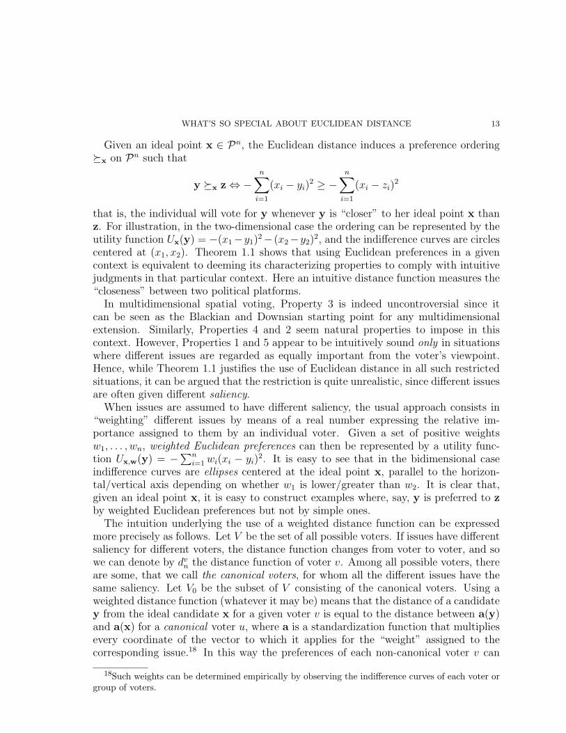
Given an ideal point x ∈ Pn, the Euclidean distance induces a preference ordering�x on Pn such that

y �x z⇔ −n∑i=1

(xi − yi)2 ≥ −n∑i=1

(xi − zi)2

that is, the individual will vote for y whenever y is “closer” to her ideal point x thanz. For illustration, in the two-dimensional case the ordering can be represented by theutility function Ux(y) = −(x1−y1)

2− (x2−y2)2, and the indifference curves are circles

centered at (x1, x2). Theorem 1.1 shows that using Euclidean preferences in a givencontext is equivalent to deeming its characterizing properties to comply with intuitivejudgments in that particular context. Here an intuitive distance function measures the“closeness” between two political platforms.

In multidimensional spatial voting, Property 3 is indeed uncontroversial since itcan be seen as the Blackian and Downsian starting point for any multidimensionalextension. Similarly, Properties 4 and 2 seem natural properties to impose in thiscontext. However, Properties 1 and 5 appear to be intuitively sound only in situationswhere different issues are regarded as equally important from the voter’s viewpoint.Hence, while Theorem 1.1 justifies the use of Euclidean distance in all such restrictedsituations, it can be argued that the restriction is quite unrealistic, since different issuesare often given different saliency.

When issues are assumed to have different saliency, the usual approach consists in“weighting” different issues by means of a real number expressing the relative im-portance assigned to them by an individual voter. Given a set of positive weightsw1, . . . , wn, weighted Euclidean preferences can then be represented by a utility func-tion Ux,w(y) = −

∑ni=1wi(xi − yi)

2. It is easy to see that in the bidimensional caseindifference curves are ellipses centered at the ideal point x, parallel to the horizon-tal/vertical axis depending on whether w1 is lower/greater than w2. It is clear that,given an ideal point x, it is easy to construct examples where, say, y is preferred to zby weighted Euclidean preferences but not by simple ones.

The intuition underlying the use of a weighted distance function can be expressedmore precisely as follows. Let V be the set of all possible voters. If issues have differentsaliency for different voters, the distance function changes from voter to voter, and sowe can denote by dvn the distance function of voter v. Among all possible voters, thereare some, that we call the canonical voters, for whom all the different issues have thesame saliency. Let V0 be the subset of V consisting of the canonical voters. Using aweighted distance function (whatever it may be) means that the distance of a candidatey from the ideal candidate x for a given voter v is equal to the distance between a(y)and a(x) for a canonical voter u, where a is a standardization function that multipliesevery coordinate of the vector to which it applies for the “weight” assigned to thecorresponding issue.18 In this way the preferences of each non-canonical voter v can

18Such weights can be determined empirically by observing the indifference curves of each voter orgroup of voters.

14 MARCELLO D’AGOSTINO AND VALENTINO DARDANONI

be represented in terms of the preferences of a canonical voter u. So, by connectingthe preferences of non-canonical voters to those of a canonical voter, one may obtaina precise mathematical expression which represents the former in terms of the latter.The advantage of this approach is that the distance function of canonical voters may bedetermined by means of some known characterization. To summarize, the assumptionunderlying the use of weighted distance functions is the following

Condition 1. For all v ∈ V and all u ∈ V0, there are αv.1, . . . , αv.n ∈ R+ such thatdvn(x,y) = dun(av(x), av(y)), where av(z) = αv.1z1, . . . , αv.nzn.

Now, this assumption leaves open how the distance function of a canonical votershould be appropriately determined. Why should weighted Euclidean distance be ap-plied and not, for instance, weighted city-block distance? Weighting, as explainedbefore, is just a way of standardizing the elements of different policy spaces into ele-ments of a reference policy space (that of a canonical voter) and tells us nothing aboutthe appropriate distance function for this reference space. Now, in the restricted do-main of canonical voters we have already argued that the distance function satisfiesProperty 1 and Property 5. Moreover, Properties 3, 2 and 4 are intuitively sound for alldvn, no matter whether v is canonical or not. Hence, we can assume that all propertiesof Theorem 1.1 are satisfied by dun, for any canonical voter u:

Condition 2. The distance function dun of any canonical voter u satisfies Properties1, 2, 3, 4 and 5.

Clearly, Conditions 1 and 2 hold true if and only if, for every v ∈ V ,

dvn(x,y) = K( n∑i=1

wi(xi − yi)2),

with wi = α2v.i and K a strictly increasing function. For, by Theorem 1.1, dun must be

monotonically related to the Euclidean distance for every canonical voter u, and so:

dvn(x,y) = dun(av(x), av(y)

)= K

( n∑i=1

(av,ixi − av,iyi

)2).

When the distance function satisfies also linear homogeneity and an appropriate nor-malization condition (see Corollary 1), K is the square root function. Thus, dvn mustbe equal to the weighted Euclidean distance, with the weight for issue i given by α2

v.i.We conclude this section by stressing that this result may be helpful in guiding

empirical research. For example [EMR88] consider weighted Euclidean distance andweighted city-block distance to determine which is empirically closer to voting behavior.By means of our analysis, empirical testing can be performed separately on each of thecharacterizing properties of Euclidean distance for a canonical voter. If these propertiesare accepted by canonical voters and Conditions 1 and 2 are considered sound, thenweighted Euclidean distance should be preferred to weighted city-block distance for allvoters. On the other hand, a direct characterization of weighted Euclidean distance fallsoutside the scope of this paper but would be an interesting topic for future research.

WHAT’S SO SPECIAL ABOUT EUCLIDEAN DISTANCE 15

5. Conclusions

As should emerge from our discussion, the results presented in Section 3 may beuseful in understanding:

• whether some suitable monotonic transformation of Euclidean Distance, in oneof the variants investigated in this paper, naturally fits a given applicationcontext, by checking whether its characterizing properties are satisfied in it(case study 1);• when the characterization results cannot be directly applied, how the original

application context can be reduced to a “canonical” one in which the propertiesof some of the characterized distance functions are all satisfied (case study 2).

Our analysis suggests that some variant of the Euclidean distance is likely to be ap-propriate in many contexts requiring a distance function which is both monotonicallyvalue-sensitive (as made precise by Properties 3/3∗ and 4) and monotonically order-sensitive (as made precise by Property 5).

6. Appendix

6.1. Proof of Theorems 1 and 2. To prove the theorems, we first need the following

Lemma 1. A distance {dn} over X satisfies Properties 1, 2, 3, 4 if and only if thereexists a continuous and strictly increasing function f : X+ → R+, with f(0) = 0, suchthat for all n ∈ N and all x,y ∈ Xn,

dn(x,y) = F[ n∑i=1

f(|xi − yi|)]

for some continuous and strictly increasing function F : R+ → R+ with F (0) = 0.

6.1.1. Proof of Lemma 1. The “if” direction is left to the reader. For the “only if”direction, we split the proof into four steps.

Step 1. Under Property 1, Property 4 is equivalent to the following:

(1) dk+j([x,u], [y,v]) ≤ dk+j([x′,u′], [y′,v′])⇐⇒ dk(x,y) ≤ dk(x

′,y′),

whenever dj(u,v) = dj(u′,v′),

for all k, j, all x,y,x′,y′ ∈ Xk and all u,v,u′,v′ ∈ Xj.

Proof. It can be easily verified that Property 4 is implied by (1). To see the converse,notice that, under Property 1, (1) is equivalent to:

(2) dk+j([x,u], [y,v]) ≤ dk+j([x′,u], [y′,v])⇐⇒ dk(x,y) ≤ dk(x

′,y′),

for all k, j, all x,y,x′,y′ ∈ Xk and all u,v ∈ Xj. We then show that, under Property 1,Property 4 implies (2), and therefore also (1).

16 MARCELLO D’AGOSTINO AND VALENTINO DARDANONI

Suppose, first, that dk+j([x,u], [y,v]) ≤ dk+j([x′,u], [y′,v]); then by Property 4 and

contrapposition, we have that dk(x,y) ≤ dk(x′,y′). On the other hand, suppose that

(i) dk(x,y) ≤ dk(x′,y′) and (ii) dk+j([x,u], [y,v]) > dk+j([x

′,u], [y′,v]).

Now, if dk(x,y) < dk(x′,y′), by Property 4, dk+j([x,u], [y,v]) < dk+j([x

′,u], [y′,v]),against the assumption (ii). If dk(x,y) = dk(x

′,y′), it follows from (ii), by Prop-erty 4 again, that d2k+j([x,u,x

′], [y,v,y′]) > d2k+j([x′,u,x], [y′,v,y]) against Prop-

erty 1. Hence, if dk(x,y) ≤ dk(x′,y′) it must hold true that dk+j([x,u], [y,v]) ≤

dk+j([x′,u], [y′,v]). �

Let us now assume that Properties 1, 2, 3, 4 hold true and recall that X can be eitherof the three intervals considered in Section 2, namely R,R+ or [0, 1].

Step 2. For all n ≥ 3 and all x,y,w, z ∈ Xn, there exists a continuous and strictlyincreasing function fn : X+ → R+, with f(0) = 0, such that

(3) dn(x,y) = Fn[ n∑i=1

fn(|xi − yi|)]

for some continuous and strictly increasing function Fn : Un → R+, with Fn(0) = 0,where Un = {u1 + · · ·+ un | ui ∈ fn(X+), i = 1, . . . , n}.

Proof. Observe that Property 3 implies

(4) d1(a, b) = d1(|a− b|, 0).

It follows from (1) that, for all n ∈ N and all x,y,w, z ∈ Xn,

(5) d1(xi, yi) = d1(wi, zi) for all i = 1, · · · , n =⇒ dn(x,y) = dn(w, z).

Therefore, given (4) above, we have that for all n and all x,y ∈ Xn,

(6) dn(x,y) = dn([|x1 − y1|, . . . , |xn − yn|], [0, . . . , 0]).

Let Mn : Xn+ → R be defined as follows

Mn(z) = dn([z1, . . . , zn], [0, . . . , 0]).

Now, since dn is assumed to be continuous, Mn must also be continuous. Moreover, itfollows from (1) and Property 3, via Property 1, that Mn is strictly increasing in eachargument zi. From (1) it also follows that, for all u,u′ ∈ Xh

+ and v,v′ ∈ Xk+, with

h+ k = n,

Mn([u,v]) ≥Mn([u′,v])⇒Mn([u,v′]) ≥Mn([u′,v′]).

So, taking into account Property 1, one can apply standard separability results ([Deb60],see also [Gor68]), to show that, for all n ≥ 3, the function Mn must be separable,19

that is, there must exist continuous and strictly increasing functions Fn : Un → R and

19See [SS02] for a recent thorough discussion on separable preferences.

WHAT’S SO SPECIAL ABOUT EUCLIDEAN DISTANCE 17

fn : X+ → R (where Un is defined as above) such that Mn(z) = Fn[∑n

i=1 fn(zi)].

Thus, by (6) and taking zi = |xi − yi|, we have that for all n ≥ 3:

(7) dn(x,y) = Fn[ n∑i=1

fn(|xi − yi|)].

We finally show that, without loss of generality, we can assume that the functions fnand Fn in (3) are such that fn(0) = 0 and Fn(0) = 0. In fact, whenever fn(0) = c 6= 0,let hn : X+ → R and Hn : R→ R be defined as hn(t) = fn(t)−c and Hn(t) = Fn(t−nc).Then, it is immediately verified that

(8) Fn[ n∑i=1

fn(|xi − yi|)]

= Hn

[ n∑i=1

hn(|xi − yi|)].

Moreover, notice that Properties 2 and 3 imply that, for all u ∈ fn(X+),

(9) Fn(u) = G(f−1n (u)).

To see this, just notice that, by Property 2, for all n ≥ 3 and for all x ∈ Xn−1,

d1(a, b) = dn([a,x], [b,x]) = Fn[fn(|a− b|) +

n−1∑i=1

fn(|xi − xi|)].

Under the assumption that fn(0) = 0 and by Property 3, we have that for all n ≥ 3,

(10) d1(a, b) = dn([a,x], [b,x]) = Fn[fn(|a− b|)] = G(|a− b|).Hence, taking u = fn(|a − b|), we obtain G(f−1

n (u)) = Fn(u). Now, to show thatFn(0) = 0, observe that fn(0) = 0 and, by Property 3, G(0) = 0, so that Fn(0) =G(0) = 0. �

Step 3. For all m,n ≥ 3, fn(t) = αm,n · fm(t), for some constant αm,n ≥ 0 dependingon m and n.

Proof. Property 2 implies immediately that for every x, y ∈ X, all n ≥ 3 and allx ∈ Xn−2, d2([x, y], [0, 0]) = dn([x, y,x], [0, 0,x]). Given Step 2, and recalling thatfor every n ≥ 3, fn(0) = 0, it follows that for every n,m ≥ 3 and every x, y ∈ X+,Fn(fn(x) + fn(y)) = Fm(fm(x) + fm(y)), and therefore, since Fn is strictly increasing,fn(x) + fn(y) = F−1

n

[Fm(fm(x) + fm(y))

]. Now, let u = fm(x) and v = fm(y); then

(considering that fm is strictly increasing):

(11) fn(f−1m (u)) + fn(f−1

m (v)) = F−1n (Fm(u+ v)).

Recall that, by (9) above, for all n ≥ 3 and all u ∈ fn(X+), Fn(u) = G(f−1n (u));

then, for all n ≥ 3, f−1n (u) = G−1(Fn(u)) and, therefore, fn(t) = F−1

n (G(t)) for allt ∈ X+. Observe also that, by (10), Fn(fn(X+)) = G(X+) for all n ≥ 3, and soran(Fm ◦ fm) ⊆ ran(Fn) for all m,n ≥ 3. Hence, for all u ∈ fm(X+),

fn(f−1m (u)) = F−1

n

(G(G−1(Fm(u))

))= F−1

n (Fm(u)),

18 MARCELLO D’AGOSTINO AND VALENTINO DARDANONI

and so, from (11):

(12) F−1n (Fm(u)) + F−1

n (Fm(v)) = F−1n (Fm(u+ v)).

Let h(t) = F−1n (Fm(t)). Then, (12) can be rewritten as:

(13) h(u) + h(v) = h(u+ v).

But (13) implies that, for all t ∈ fm(X+),

(14) h(t) = F−1n (Fm(t)) = αm,n · t

for some constant αm,n ≥ 0 depending on m and n.20 Moreover, since Fm and Fn arestrictly increasing, so are F−1

n and F−1n ◦ Fm; therefore αm,n > 0.

Now, by Property 2 again, it follows that for every x ∈ X+, all m,n ≥ 3 with m ≤ n,all u ∈ Xm−1 and all v ∈ Xn−1,

(15) dm([x,u], [0,u]) = dn([x,v], [0,v]).

Therefore, by (3), for every x ∈ X+ and all m,n ≥ 3 with m ≤ n, Fm(fm(x)) =Fn(fn(x)), and so, by (14)

(16) fn(x) = F−1n (Fm(fm(x))) = αm,n · fm(x).

�

We now show that Property 2 allows us to replace the functions Fn and fn in (3) withsuitable functions F and f which are independent of n, and to extend (3) to the caseswhere n < 3.

Step 4. There exists a continuous and strictly increasing function f : X+ → R+, withf(0) = 0, such that for all n and all x,y ∈ Xn,

dn(x,y) = F[ n∑i=1

f(|xi − yi|)]

for some continuous and strictly increasing function F : R+ → R+ with F (0) = 0.

Proof. Let f be equal to f3 and let αn be the appropriate constant satisfying (14) form = 3 and a given n ≥ 3. Let also F ′n(t) = Fn(αn · t). Then, it follows from Step 2and (16) that for all n ≥ 3 and all x,y ∈ Xn:

(17) dn(x,y) = Fn[ n∑i=1

fn(|xi − yi|)]

=

= Fn[αn

n∑i=1

f(|xi − yi|)]

= F ′n[ n∑i=1

f(|xi − yi|)],

where F ′n(t) is continuous and strictly increasing. Moreover, by Property 2,

(18) dn(x,y) = dn+1([x, z], [y, z])

20(13) is a Cauchy equation of the first kind whose solution is given, for example, in Aczel [Acz66].

WHAT’S SO SPECIAL ABOUT EUCLIDEAN DISTANCE 19

for all z ∈ X, and since

(19) dn+1([x, z], [y, z]) = Fn+1

[ n∑i=1

fn+1(|xi − yi|) + fn+1(0)]

=

= Fn+1

[ n∑i=1

fn+1(|xi − yi|)]

= Fn+1

[αn+1

n∑i=1

f(|xi − yi|)]

= F ′n+1

[ n∑i=1

f(|xi − yi|)],

it follows from (17), (18) and (19) that F ′n+1(u) = F ′n(u) for all u ∈ dom(F ′n).Therefore, F =

⋃∞i=3 F

′i is a function from

⋃∞i=3 dom(F ′i ) = R+ in R+. Then F is

continuous and strictly increasing, since all the F ′i are, and dn(x,y) = F[∑n

i=1 f(|xi−yi|)]

for all n ≥ 3. To conclude the step then observe that, when x and y have sizek < 3, by Property 2 and recalling that f(0) = 0, it follows that for any z ∈ Xm:

(20) dk(x,y) = dk+m([x, z], [y, z]) = F[( k∑

i=1

f(|xi − yi|) +k+m∑j=k+1

f(|zj − zj|))]

=

= F( k∑i=1

f(|xi − yi|)),

and so the identity dn(x,y) = F[∑n

i=1 f(|xi − yi|)]

holds for all n ∈ N. Finally,F (0) = Fn(αn · 0) = Fn(0) and, by Step 2, Fn(0) = 0, so F (0) = 0. �

6.1.2. Proof of Theorem 1. Given the above lemma, to prove the “if” direction of The-orem 1.1 it is sufficient to verify that any strictly increasing function of the Euclideandistance satisfies Property 5, that is, to verify that, whenever (xi − xj)(yi − yj) > 0,(xk − xm)(yk − ym) > 0, d1(xi, xj) = d1(xk, xm) and d1(yi, yj) ≤ d1(yk, ym), we have

(21) (xi − yj)2 + (xj − yi)2 + (xk − yk)2 + (xm − ym)2 ≤≤ (xi − yi)2 + (xj − yj)2 + (xk − ym)2 + (xm − yk)2.

After simplification, this equation becomes (xm − xk)(ym − yk) ≥ (xj − xi)(yj − yi),and the result follows. To prove the “only if” direction, we need to show that thefunction f in Lemma 1 must be quadratic. Let a, b, c ∈ X be arbitrary non negativereal numbers with a ≥ c. Let also x,y ∈ X4 be such that

x = [a, (a+ c), a, (a+ c)], y = [0, c, a, (a+ c)]

so thatσ12(y) = [c, 0, a, (a+ c)], σ34(y) = [0, c, (a+ c), a].

Let σ12(y) = w and σ34(y) = z. Since (x1 − x2)(y1 − y2) > 0, (x3 − x4)(y3 − y4) >0, d1(x1, x2) = d1(x3, x4) and d1(y1, y2) = d1(y3, y4), by Property 5 it follows thatd4(x,w) = d4(x, z); hence, by Lemma 1, we have that

F( 4∑i=1

f(|xi − wi|))

= F( 4∑i=1

f(|xi − zi|))

20 MARCELLO D’AGOSTINO AND VALENTINO DARDANONI

and therefore, since F is strictly increasing,∑4

i=1 f(|xi − wi|) =∑4

i=1 f(|xi − zi|).Hence, subtracting

∑4i=1 f(|xi − yi|) from both sides, we obtain

4∑i=1

f(|xi − wi|)−4∑i=1

f(|xi − yi|) = f(a+ c) + f(a− c)− 2f(a)

and

4∑i=1

f(|xi − zi|)−4∑i=1

f(|xi − yi|) = 2f(c)− 2f(0).

Therefore, recalling that f(0) = 0, we must have for all a ≥ c ≥ 0:

f(a+ c)− f(a) = f(a)− f(a− c) + 2f(c)

This functional equation has a unique solution f(t) = αt2 for some constant α > 0.Hence, from Lemma 1, it follows that dn(x,y) = F

[α ·∑n

i=1(xi − yi)2]. Since

F (α · u) is strictly increasing in u and F (α · 0) = F (0) = 0, this concludes the proof ofthe theorem.

To prove Theorem 1.2, just replace Lemma 1 with the following:

Lemma 2. A distance {dn} over X satisfies Properties 1, 2∗, 3, 4, if and only if thereexists a continuous and strictly increasing function f : X+ → R+, with f(0) = 0,such that for all n ∈ N and all x,y ∈ Xn, dn(x,y) = F

[1n

∑ni=1 f(|xi − yi|)

]for some

continuous and strictly increasing function F : f(X+)→ R+ with F (0) = 0.

Its proof is equal to that of Lemma 1 up to Step 2, and thereafter continues as follows.Let gn = nfn, so that

(22) dn(x,y) = Mn(|x1 − y1|, · · · , |xn − yn|) = Fn[ n∑i=1

1

ngn(|xi − yi|)

].

Then, following the derivation of equation (21) from equation (14) in Foster andShorrocks [FS91], we have that Property 2∗ allows us to choose the functions Fnand gn to be independent of n (i.e. such that for all m,n ∈ N, Fm = Fn = F andgm = gn = f , for some fixed F and f) and to extend (22) to the case of n < 3. Thusdn(x,y) = F

[1n

∑ni=1 f(|xi− yi|)

]holds for all n ∈ N. Then, a proof of the second part

of the theorem can be obtained by using Lemma 2 instead of Lemma 1 and adaptingthe previous proof accordingly.

6.1.3. Proof of Theorem 2. A proof of Theorem 2 could be obtained using a similarargument, based on separability properties, as the one used in the proof of Theorem 1Here we suggest how to obtain a simpler proof which uses Theorem 1 as a lemma.

First, (1) implies that for all n ∈ N and all x,y,w, z ∈ Xn,

d1(xi, yi) = d1(wi, zi) for all i = 1, · · · , n,=⇒ dn(x,y) = dn(w, z).

This means that dn(x,y) = Fn(d1(x1, y1), . . . , d1(xn, yn)) for some function Fn; more-over, it also follows from (1) and Property 1, that Fn is strictly increasing in each

WHAT’S SO SPECIAL ABOUT EUCLIDEAN DISTANCE 21

argument. Now, by Property 3∗, di(xi− yi) = G(|g(xi)− g(yy)|), with G and g strictlyincreasing. Hence dn(x,y) = Hn(|g(x1) − g(y1)|, . . . , |g(xn) − g(yn)|) for some strictlyincreasing Hn.

Now, let d′n be defined as follows:

d′n(u,v) = dn(g−1(u),g−1(v)) = Hn(|u1 − v1|, . . . , |un − vn|),

where g−1(z) stands for the vector [g−1(z1), . . . , g−1(zn)]. Clearly, d′n satisfies Proper-

ties 1, 2 and 4 whenever dn does. Moreover, it is not difficult to verify that, wheneverdn satisfies Properties 3∗ and 5, d′n satisfies Properties 3 and 5. Therefore, wheneverdn satisfies all the properties of Theorem 2.1, d′n satisfies all the properties of Theo-rem 1.1, and we can apply this theorem to establish that d′n must be (some monotonictransformation of) the Euclidean Distance. Thus, writing g(z) for [g(z1), . . . , g(zn)],we have

dn(x,y) = d′n(g(x),g(y)) = H( n∑i=1

(g(xi)− g(yi))2)

for some strictly increasing H such that H(0) = 0. Similarly, whenever dn satisfies allthe properties of the Theorem 2.2, d′n satisfies all the properties of Theorem 1.2, and wecan apply this theorem to establish that d′n must be (some monotonic transformationof) the Averaged Euclidean Distance, that is dn(x,y) = H

[1n

∑ni=1(g(xi)− g(yi))

2]

forsome strictly increasing H such that H(0) = 0.

References

[Acz66] J. Aczel. Lectures on functional equations and their applications. Accademic Press, NewYork, 1966.

[ASB99] D. Austen-Smith and J.S Banks. Positive Political Theory I: Collective Preference. TheUniversity of Michigan Press, 1999.

[Atk83] A.B. Atkinson. The measurement of economic mobility. In A.B. Atkinson, editor, SocialJustice and Public Policy. Wheatsheaf Books Ltd., London, 1983.

[Bri50] G.W. Brier. Verfication of forecasts expressed in terms of probability. Monthly WeatherReview, 78:1–3, 1950.

[Cow85] F. Cowell. Measures of distributional change: An axiomatic approach. Review of Eco-nomic Studies, 52:35–51, 1985.

[Dar93] V. Dardanoni. Measuring social mobility. Journal of Economic Theory, 61:372–94, 1993.[Deb60] G. Debreu. Topological methods in cardinal utility. In S. Karlin K. Arrow and P. Suppes,

editors, Mathematical methods in the social sciences. Stanford University Press, 1960.[EMR88] J.M. Enelow, N.R. Mendell, and S. Ramesh. A comparison of two distance metrics

through regression diagnostics of a model of relative candidate evaluation. The Jour-nal of Politics, 50:1057–1071, 1988.

[ET80] L.G. Epstein and S.M. Tanny. Increasing generalized correlation: A definition and someeconomic consequences. Canadian Journal of Economics, 13:16–34, 1980.

[FO96] G.S. Fields and E. Ok. The meaning and measurement of income mobility. Journal ofEconomic Theory, 71:349–77, 1996.

[FO99a] G.S. Fields and E. Ok. The measurement of income mobility. In J. Silber, editor, Handbookof Income Inequality Measurement. Kluwer Academic Publishers, Dordrecht, 1999.

[FO99b] G.S. Fields and E. Ok. Measuring movements of incomes. Economica, 66:455–71, 1999.

22 MARCELLO D’AGOSTINO AND VALENTINO DARDANONI

[FS91] J.E. Foster and A.F. Shorrocks. Subgroup consistent poverty indices. Econometrica,59:687–709, 1991.

[FS97] J.E. Foster and A. Sen. On economic inequality after a quarter century. In A. Sen, editor,On Economic Inequality. Clarendon Press, Oxford, 1997.

[Gor68] W.M. Gorman. The structure of utility functions. Review of Economic Studies, 35:367–390, 1968.

[HM70] M.J. Hinich and M.C. Munger. Analytical Politics. Cambridge University Press, Cam-bridge, UK, 1970.

[Maa98] E. Maasoumi. On mobility. In D. Giles and A. Ullah, editors, The Handbook of EconomicStatistics. Marcel Dekker, New York, 1998.

[MO98] T. Mitra and E. Ok. The measurement of income mobility: A partial ordering approach.Economic Theory, 12:77–102, 1998.

[Sho88] A.F. Shorrocks. Aggregation issues in inequality measurement. In W. Eichhorn, editor,Measurement in Economics. Springer Verlag, New York, 1988.

[SJ99] S. Santini and R. Jain. Similarity measures. IEEE Transactions on Pattern Analysis andMachine Intelligence, 21(9):871–883, 1999.

[SS02] U. Segal and J. Sobel. Min, max, and sum. Journal of Economic Theory, 25:126–150,2002.

[Tch80] A.H.T. Tchen. Inequalities for distributions with given marginals. Annals of Probability,8:814–27, 1980.

[TJaLA01] Wu T-J. and Hsieh Y-C. andLi L-A. Statistical measures of dna sequence dissimilarityunder markov chain models of base composition. Biometrics, 57:441–448, 2001.

[TK70] Amos Tverski and David H. Krantz. The dimensional representation and the metricstructure of similarity data. Journal of Mathematical Psychology, 7:572–596, 1970.

[VdGSM01] D. Van de Gaer, E. Schokkaert, and M. Martinez. Three meanings of intergenerationalmobility. Economica, 68:519–537, 2001.

[WBD97] Tiee-Jian Wu, John P. Burke, and Daniel B. Davison. A measure of dna sequence dissimi-larity based on mahalanobis distance between frequencies of words. Biometrics, 53:1431–1439, 1997.

[WZF05] Liwei Wang, Yan Zhang, and Jufu Feng. On the euclidean distance of images. IEEETransactions on Pattern Analysis and Machine Intelligence, 27:1334–1339, 2005.

Dipartimento di Scienze Umane, Universita di FerraraE-mail address: dgm@unife.it

Dipartimento di Scienze Economiche, Aziendali e Finanziarie, Universita di PalermoE-mail address: vdardano@unipa.it