Seediscussions,stats,andauthorprofilesforthispublicationat:https://www.researchgate.net/publication/45901895

Spinorsineuclideanfieldtheory,complexstructuresanddiscretesymmetries

ArticleinNuclearPhysicsB·February2010

DOI:10.1016/j.nuclphysb.2011.06.013·Source:arXiv

CITATIONS

22

READS

26

1author:

ChristofWetterich

UniversitätHeidelberg

316PUBLICATIONS14,598CITATIONS

SEEPROFILE

AllcontentfollowingthispagewasuploadedbyChristofWetterichon01December2016.

Theuserhasrequestedenhancementofthedownloadedfile.Allin-textreferencesunderlinedinbluearelinkedtopublicationsonResearchGate,lettingyouaccessandreadthemimmediately.

arX

iv:1

002.

3556

v1 [

hep-

th]

18

Feb

2010

Spinors in euclidean field theory,

complex structures and discretesymmetries

C. Wetterich

Institut fur Theoretische PhysikUniversitat Heidelberg

Philosophenweg 16, D-69120 Heidelberg

Abstract

We discuss fermions in arbitrary euclidean dimensions. Particular empha-sis is given to the definition of generalized Majorana spinors in four dimen-sions. They can be associated to a new complex structure which involvesa reflection in euclidean time. These objects permit a consistent analyticcontinuation of Majorana spinors in Minkowski space to euclidean signature,avoiding a doubling of degrees of freedom. We discuss rotation invariantderivative and interaction terms in the action, noting that the rotations can-not be expressed in a complex basis with respect to the new complex structure.The possible complex structures for Minkowski and euclidean signature canbe understood in terms of a modulo two periodicity in the signature. We alsodiscuss the discrete symmetries of parity, time reversal and charge conjugationfor arbitrary dimension and signature.

1 Introduction

Analytic continuation from Minkowski signature to euclidean signature is a centraltool in quantum field theory. Many non-perturbative computations, as lattice gaugetheory for quantum chromodynamics, are directly performed in euclidean space-time. For fermions, the mapping between Minkowski space and euclidean spaceis, however, not without problems. The basic issue is a modulo two periodicityin signature for the reality properties of representations of the generalized Lorentzgroup. While the two fundamental spinor representations 2L,R of the Lorentz groupin four dimensions are complex, the fundamental spinors 21, 22 are (pseudo)-real forthe orthogonal group SO(4). Complex conjugation maps the spinor representationsof SO(1, 3) into each other, 2L ↔ 2R, while the SO(4)-spinors 21 and 22 are mappedinto themselves.

This simple property has important consequences for the definition of chargeconjugation and Majorana spinors, as needed, for example, for the mass eigenstates

of the neutrinos. Usually, Majorana spinors are associated to real 2[d2 ]-component

spinor representations of the generalized d-dimensional Lorentz group (with[d2

]=

(d − 1)/2 for odd). For Minkowski signature, they exist for d = 2, 3, 4, 8, 9 mod 8[1]. (In four dimensions, a four-component Majorana spinor can be associated to atwo-component complex Weyl spinor - the four real components can be obtained aslinear combination of the real and imaginary parts of the Weyl spinors.) A similarprescription for euclidean signature allows Majorana spinors for d = 2, 6, 7, 8, 9. Noeuclidean Majorana spinor exists for d = 4 according to this definition.

It is sometimes advocated that the number of spinor degrees has to be doubled iffour-dimensional Majorana or Weyl spinors are described with euclidean signature.From the point of view of analytic continuation this is obviously not a very satisfac-tory situation. Continuity is not compatible with a sudden jump of the number ofdegrees of freedom. We propose here that no such doubling is necessary. To everymodel in Minkowski space corresponds a euclidean model with the same number ofspinor degrees of freedom. What has to be questioned, however, is the implemen-tation of the discrete symmetries like charge conjugation, and correspondingly thenotion of the complex structure.

We introduce a generalized notion of Majorana spinors which make euclideanand Minkowski signature compatible. This also leads to a generalized concept of“reality” of the action, closely related to the old observation that hermiticity forthe action in Minkowski space corresponds to Osterwalder-Schrader positivity ineuclidean space [2]. The notion of “reality” of a spinor is no longer linked to therepresentation theory of the generalized Lorentz group, but rather to eigenstatesof a generalized charge conjugation. Similar remarks actually apply to the chiralantisymmetric tensor representation of rank d/2 (for even dimensions), where thereality properties also jump with a modulo two periodicity in the signature [3].

We present a unified picture of the discrete symmetries parity, time reversaland charge conjugation for arbitrary dimension and signature. It reflects directly

1

the property that charge conjugation in euclidean space involves a reflection ineuclidean time and the zero-component of momentum q0. With t the Minkowskitime and τ = it the euclidean time, the complex conjugation (it)∗ = −it = −τindeed results in τ → −τ . Similarly, the complex conjugation in euclidean space,τ → τ ∗, is mapped to time reflection t → −t in Minkowski space. As a byproductof our investigation, we develop a consistent notation for spinors in arbitrary d andfor arbitrary signature.

In sect. 2 we start with basic notions of spinor fields in the functional integralapproaches to quantum field theory. We discuss analytic continuation in sect. 3and the usual notion of complex conjugation in Minkowski space in sect. 4. Weinterprete this as a mapping θM in the space of spinor components. In sect. 5 weintroduce the analogous mapping θ in euclidean space. It includes a reflection of thetime coordinate. We discuss an important modulo two periodicity in the signature,by which the role of θ and θM are switched as the number of timelike dimensionsincreases by one unit. In particular, the map θ for euclidean signature induces thesame type of map between the Weyl spinors as θM does for Minkowski signature.

In sect. 6 we describe a generalized complex conjugation for spinors with eu-clidean signature. It is based on the map θ and therefore involves an additionalreflection of the zero-component of the momentum or a reflection of euclidean time.This is used in sect. 7 in order to define a real action as a Grassmann element that isinvariant under the combination of the transformation θ or θM and a total reorder-ing of all Grassmann variables (transposition). The functional integral with a realaction yields a real result. We generalize this discussion to the possible presence ofbosonic fields in addition to the fermionic spinors. In sect. 8 we discuss hermiteanspinor bilinears which can be used in order to construct a real action for providingobservables that have a real expectation value.

In sects. 9, 10 we turn to the proper definition of physical Majorana andMajorana-Weyl spinors for euclidean signature. These do not coincide with thereal spinor representations of the rotation group SO(d). We define in sect. 9 ageneralized charge conjugation which maps the spinor ψ to its conjugate spinor ψ.If this map defines an involution CW we can define in sect. 10 the generalized Ma-jorana spinors as the eigenstates of CW with eigenvalues +1 or −1. For Majoranaspinors the Grassmann variables ψ and ψ in the functional integral are no longer in-dependent, ψ can be expressed in terms of ψ. The generalized Majorana constraintreduces the number of degrees of freedom by a factor two, as expected for Majoranaspinors. For Minkowski signature the generalized Majorana spinors coincide withthe usual notion of Majorana spinors. We define physical Majorana spinors by theconstraint that an invariant kinetic term in the action should be allowed. Physi-cal Majorana spinors exist for d = 2, 3, 4, 8, 9 mod 8, and physical Majorana-Weylspinors are allowed for d = 2 mod 8. The existence of physical Majorana spinorstherefore depends only on the dimension d, and not on the signature s. In particular,analytic continuation between Minkowski and euclidean signature is always possiblefor physical Majorana and Majorana-Weyl spinors.

2

In sect. 11 we extend our discussion to the appropriate definitions of parity andtime reversal which are compatible with analytic continuation. These symmetriescan be defined consistent with the Majorana constraint and with analytic contin-uation. In sect. 12 we address possible continuous internal symmetries acting onthe spinors. For N species of Dirac spinors the kinetic term is invariant under thegroup SL(2N,C) of regular complex 2N × 2N matrices. The chiral transforma-tions U(N)× U(N) are a subgroup of this group. While the chiral transformationsare compatible with the complex structure, this does not hold for the generalizedSL(2N,C) transformations. We present our conclusions in sect. 13. Detailedconventions for four dimensions are collected in appendix A and a short generaldiscussion of possible complex structures for a real or complex Grassmann algebrais given in appendix B.

2 Spinor degrees of freedom

Let us consider an arbitrary number of dimensions d with arbitrary signature s,where the diagonal metric ηmn has d−s eigenvalues +1 and s eigenvalues −1. Laterwe will concentrate on the euclidean case s = 0 and compare it with a Minkowskisignature s = 1 (or s = d− 1). We start with Dirac spinors described by associatedelements of a Grassmann algebra ψ and ψ. This Grassmann algebra is generatedby two sets of independent Grassmann variables ψu and ψv which fulfill the usualanticommutation relations

ψu, ψv = ψu, ψv = ψu, ψv = 0. (2.1)

We may choose ψu ≡ ψaγ(x) or ψu ≡ ψaγ(q) in a coordinate or momentum represen-tation. Here γ are the “Lorentz-indices” on which the generalized Lorentz groupSO(s, d − s) acts, while the index a denotes further possible internal degrees offreedom or different species of Dirac spinors.

Integration and differentiation with Grassmann variables obey the usual rules

∫dψug =

∂

∂ψug ,

∫dψuψv = δuv,

∫dψuψv =

∫dψu = 0

∂

∂ψu,∂

∂ψv = 0, dψu, dψv = 0 (2.2)

such that ∫ ∏

u′

(dψu′dψu′) exp(ψuAuvψv) = det A. (2.3)

Elements of the Grassmann algebra are sums of products of Grassmann variableswith complex coefficients. Spinors are elements of the Grassmann algebra whichare linear in ψu or ψv. In particular, for a Dirac spinor one has ψ =

∑u auψu, ψ =

3

∑v bvψv, with ψ

2 = 0, ψ2 = 0, ψ, ψ = 0. For example, a spinor wave function inposition space can be expressed in terms of the Grassmann variables ψaγ(q) by

ψaγ(x) =∑

q

exp(iqµxµ)ψaγ(q). (2.4)

We can consider ψaγ(x) as new Grassmann variables obeying eqs. (2.1), (2.2) suchthat eq. (2.4) amounts to a change of basis for the Grassmann algebra. Indeed, everyregular linear transformation A defines a new set of Grassmann variables,

ϕi = Aijψj ,d

dϕk= A−1

jk

d

dψj,

d

dϕkϕi = δki. (2.5)

Every complete set of spinors can be taken as a complete set of Grassmann variableswhich defines a basis for the Grassmann algebra. We observe that the Grassmannalgebra G is defined over the complex numbers, i.e. λg is defined for all g ∈ G andλ ∈ C, but we do not assume a priori the existence of a complex conjugation withinG, i.e. g∗ (or ψ∗) is not necessarily defined.

We define the “functional measure”∫

DψDψ =

∫ ∏

u′

(dψu′dψu′) (2.6)

and the partition function

Z =

∫DψDψ exp

(− SE [ψ, ψ]

). (2.7)

Here the euclidean action SE is a polynomial of an even number of Grassman vari-ables. (For s = 1, SE will be related to the “Minkowski action” SM by SE = −iSM .)The action may contain appropriate source terms such that Z becomes the generat-ing functional for Greens functions in the standard way.

A Dirac spinor has 2[d2] components labeled by the spinor index γ with [d

2] = d

2

for d even and [d2] = d−1

2for d odd. The spinor ψγ transforms under generalized

infinitesimal Lorentz transformations as1

δψγ = −1

2ǫmn(Σ

mn) δγ ψδ. (2.8)

Here the generators Σmn of the group SO(s, d−s) are related to the Clifford algebraby

Σmn = −1

4[γm, γn] , γm, γn = 2ηmn, (2.9)

1Here ǫmn = −ǫnm = ǫ∗mn and the index m runs from 0 to d − 1 in order to be close tostandard Minkowski space notation. For an euclidean signature s = 0 the Lorentz transformationscorrespond to standard SO(d) rotations.

4

with (γm)† = γm for ηmm = 1 and (γm)† = −γm for ηmm = −1. (Hermiteangenerators can be obtained from Σmn by suitable multiplication of factors i.) Wepostulate that an infinitesimal Lorentz transformation of ψ reads

δψ =1

2ǫmnψΣ

mn. (2.10)

Then the bilinears ψψ, ψγmψ, ψΣmnψ etc. transform as Lorentz scalars, vectors,second rank antisymmetric tensors and so on. A Lorentz-invariant action can beconstructed from these building blocks.

In even dimensions Dirac spinors are reducible representations. They may bedecomposed into Weyl spinors with the d-dimensional generalization of the γ5-matrixγ defined by

γ = ηγ0γ1...γd−1 = −ηγ1 · · ·γd−1γ0. (2.11)

We require γ2 = 1 such that (1± γ)/2 are projectors. This implies for the phase η

η2 = (−1)d2−s. (2.12)

With this phase γ is hermitean. The matrix γ anticommutes with all Dirac matricesγm and therefore indeed commutes with Σmn. We summarize the properties of γ by

γ2 = 1, γ† = γ, γm, γ = 0, [Σmn, γ] = 0. (2.13)

Finally, we fix the phase as

η = (−i)d2−s. (2.14)

Weyl spinors 2 are defined as ψ± = 12(1± γ)ψ.

The spinor kinetic term3

Skin =

∫ddxψ(iγµ∂µ)ψ (2.15)

is invariant under both Lorentz and internal U(N) transformations. (Gauge invari-ance and general coordinate invariance can be implemented as usual by employingcovariant derivatives instead of ∂µ.) We emphasize that the kinetic term is given byeq. (2.15) for arbitrary signature and arbitrary dimension. This fixes4 the relativephase convention between ψ and ψ.

In even dimensions a Dirac spinor is composed from two Weyl spinors withopposite “helicity”

ψ± =1

2(1± γ)ψ , ψ± =

1

2ψ(1∓ γ). (2.16)

2In analogy to the four dimensional notation in Minkowski space one may identify ψ+ =ψL, ψ− = ψR.

3For flat space one has γµ = δµmγm, whereas for more general geometries the vielbein eµm replaces

δµm.4Different conventions for the kinetic term can be related to ours by multiplication of ψ with a

phase or with γ.

We have chosen here conventions for ψ± such that ψ+ψ+ = 0, ψγmψ = ψ+γmψ+ +

ψ−γmψ− as one is used to from Minkowski space in four dimensions5. The kinetic

term (2.15) decomposes then into independent kinetic terms for the Weyl spinorsψ+ and ψ−

Skin =

∫ddx

ψ+(iγ

µ∂µ)ψ+ + ψ−(iγµ∂µ)ψ−

. (2.17)

For arbitrary signature it is invariant under separate “chiral rotations” of ψ+ andψ−. Such a chiral rotation acting only on ψ+

ψi+ −→ U ijψ

j+ , ψi− −→ ψi− (2.18)

must transform ψ± according to

ψi+ −→ ψ j+ (U †) ij , ψi− −→ ψi−. (2.19)

The Weyl spinors ψ+ and ψ+ correspond to inequivalent spinor representations ofthe Lorentz group in d = 4 mod 4, and to equivalent ones in d = 2 mod 4.

3 Analytic continuation

The Minkowski signature s = 1 and euclidean signature s = 0 can be connectedby analytic continuation. Rather than continuing the time coordinate we will usehere a formulation with a vielbein. The analytic continuation multiplies the 0−m-components of the vielbein with a phase. (This is, of course, equivalent to the usualcontinuation of time.)

Let us start with euclidean signature with a free massless Dirac spinor

SE = Skin = i

∫ddxeψγmem

µ∂µψ (3.1)

with vielbein eµm = δmµ , inverse vielbein e

µm obeying em

µeµn = δnm and e = det(eµ

m).We may now consider eµ

m as a free variable on which the partition function depends.In particular, we consider the choice for the vielbein

e0m = eiϕδm0 , ek

m = δmk , k = 1 . . . d− 1. (3.2)

Correspondingly, one has e = eiϕ and the inverse vielbein obeys em0 = e−iϕδ0m, em

k =δkm. We observe that Skin does not depend on ϕ. (Remember that we do neithertransform the coordinates nor the Grassmann variables ψ, ψ.) As usual in generalrelativity we define the matrices

γµ = γmemµ, γµ, γν = em

µenνδmn = gµν . (3.3)

5Note that ψ+ denotes here the “plus component of ψ” rather than the Lorentz representationwhich is the complex conjugate to the Weyl spinor ψ+. The latter would be (ψ+) =

12 ψ(1+(−1)sγ)

[1]. In this respect our notations differ from ref. [1]

6

If we specialize to ϕ = π/2, eiϕ = i, we find gµν = ηµνM where ηµνM has now theMinkowski signature s = 1, i.e. η00M = −1. Correspondingly, we may identify theDirac matrices γµ with the matrices defined by eq. (2.9) for s = 1. This also holdsfor Σµν = −1

4[γµ, γν ] which now generates the Lorentz group SO(1, d− 1). In short,

the theory with s = 1 (and vielbein eµm = δmµ ) can be seen equivalently as a theory

with euclidean signature (s = 0) and complex vielbein given by (3.2).For the Dirac algebra the only change from euclidean to Minkowski signature is

therefore the relationγ0M ≡ γµ=0

M = −iγ0E . (3.4)

The matrix γ remains identical for both euclidean and Minkowski signature sinceby virtue of eq. (2.14) one finds for s = 1 the phase ηM = iηE . We may replace inthe definition (2.11), (2.14) the factor is by e,

γ = (−i)d2 e∏

µ

γµ = (−i)d2

∏

m

γm, (3.5)

with properly ordered and symmetrized products. This clearly shows that γ is notaffected by analytic continuation.

For euclidean signature the natural definition of the action is S(s=0)E =

∫d4xeELE

with eE = 1 in flat space. For a Minkowski signature the historical conventioncontains an additional minus sign S

(s=1)M =

∫d4xLM = −

∫d4xLE (anal. contd),

corresponding to LM ∼ kinetic energy minus potential energy (T −V ). (V does notchange under analytic continuation). This implies

S(s=1)M = iS

(s=0)E (anal. contd.) (3.6)

where a factor i accounts for the fact that the definition of SE (anal. contd.) includesthe analytical continuation of the volume element e which is not included in thedefinition of SM . The analytical continuation of LE can either be realized by achange from euclidean to Minkowski γm-matrices with a simultaneous change ofthe signature for ηmn. Alternatively, one may keep γm and ηmn fixed and performthe analytical continuation in the vielbein.6 Going from euclidean to Minkowskisignature the weight factor in the partition function changes then only by a changeof the “background” vielbein, with exp(iSM) = exp(−S

(s=0)E (anal. contd)). In

particular, if one would construct gravity theories where the vielbein is a complexintegration variable one has the same weight factor for all signatures. This also holdsfor theories where no explicit vielbein or ηmn appears, like for spinor gravity [4]. Forboth procedures the analytical continuation of γµ = γme µ

m and gµν = 12γµ, γν is

the same.

6In flat space the analytic continuation in the vielbein can be replaced by an analytic continu-ation in the time variable. Our convention corresponds to t = −iτ , with τ/t the time variable ineuclidean/Minkowski space, respectively.

7

4 Complex conjugation for Minkowski signature

In Minkowski space we are used to the notion of a complex conjugation which relates7

ψ∗ and ψψ = ǫDTψ∗ , ǫ2 = 1. (4.1)

Here the matrix D acts only on spinor indices and obeys for even d

DΣmnD−1 = −(Σmn)† , D†D = 1. (4.2)

These conditions can be fulfilled if D is given either by D1 or D2 which obey

D1γmD−1

1 = (γm)† , D2γmD−1

2 = −(γm)†,

D †1 = D1 , D

†2 = −D2 , D2 = is−1D1γ. (4.3)

The matrix D1 is given by D1 = 1, γ0γ, γ0, γ for s = 0, 1, d− 1 and d, respectively,with γ0 = γ0† for s = d − 1 and γ0 = −γ0† for s = 1. The kinetic term (2.15) ishermitean (cf. sect. 5) for both D1 and D2. Eq. (4.1) defines the notion of thecomplex conjugate spinor which has not yet been introduced so far. It is an elementof the Grassmann algebra which can be written in terms of ψ as

ψ∗ = ǫ(DT )−1ψ. (4.4)

We will see later that other definitions are also possible.A linear transformation

ψ(x) −→ Aψ(x′) (4.5)

is compatible with this complex conjugation if

ψ∗(x) → A∗ψ∗(x′) (4.6)

or if the associated spinor ψ transforms as

ψ(x) −→ ψ(x′)D−1A†D. (4.7)

We conclude that Lorentz transformations are compatible with the complex con-jugation. Another example is a unitary matrix A acting only on internal indicesa = 1...N with ψ → ψA†. Then the spinor ψ transforms as the complex conjugaterepresentation of ψ with respect to the corresponding symmetry group (U(N) ora subgroup of it) and ψψ is invariant. We emphasize that transformations A not

7We will not always make a distinction between ψ and ψT such that we may also write ψ = ǫψ†D.In order to avoid confusion with ref. [1] we emphasize that in [1] ψ denotes the complex conjugateof ψ in a group-theoretical sense for which (4.1) holds for arbitrary signature. In the present paperψ denotes the spinor associated to ψ by the kinetic term (2.15). The introduction of ǫ is motivatedby standard conventions for charge conjugate spinors to be explained later. Both D and ǫD obeythe relation (4.2).

8

obeying the compatibility condition (4.7) or even more general transformations mix-ing ψ and ψ remain well defined. They simply do not obey the rule (4.6) and cantherefore not be written as complex matrix multiplication for complex spinors. Wewill see in sect. 6 that there is an option to define a complex conjugation differentfrom (4.1) in case of an euclidean signature.

Using the identityD−1γD = (−1)sγ = (−1)d−sγ (4.8)

we see that the chiral transformations (2.18) are compatible with eq. (4.7) onlyif the number of dimensions with negative signature is odd. This indicates thatthe association (4.1) of ψ with the complex conjugate of ψ is not compatible withchiral rotations for a euclidean signature. Only for a Minkowski signature the usualdefinition of the complex conjugate spinor ψ∗ according to (4.1) is compatible withthe chiral rotations. The incompatibility of the identification (4.1) with the chiralstructure of the theory is well known and translates a simple property of the spinorrepresentations of the generalized Lorentz group SO(s, d−s) with respect to complexconjugation: In four dimensions and for Minkowski signature (s = 1 or 3) the twoinequivalent irreducible spinor representations 2L and 2R are complex conjugateto each other. For an euclidean signature (s = 0 or 4) the corresponding spinorrepresentations of SO(4) are (pseudo)real.

A spinor bilinear transforming as a four vector (2L, 2R) cannot be formed froman irreducible two-component spinor and its complex conjugate if the signatureis euclidean and complex conjugation is defined by eq. (4.4). Similar features andcomplications generalize to all even dimensions. This observation has often led to theopinion that the spinor degrees must be doubled when the signature is changed fromMinkowski to euclidean. We emphasize, however, that the number of independentspinors ψ a

γ (q), ψ aγ (q) is exactly the same for all signatures. Only the standard

complex structure in the Grassmann algebra which defines ψ∗ in the usual way (4.1)is not compatible with chiral rotations for a euclidean signature.

The complex and hermitean conjugates of an element g of the Grassmann alge-bra8

g = aγ1...γp δ1...δqu1...up v1...vqψ

u1γ1ψ

u2γ2 ...ψ

upγp ψ

v1δ1...ψ

vqδq (4.9)

are defined by

g∗ = (aγ1...γpδ1...δqu1...upv1...vq)∗(ψu1γ1 )

∗...(ψupγp )∗(ψv1δ1 )

∗...(ψvqδq)∗,

g† =(aγ1...γp δ1...δqu1...up v1...vq

)∗ (ψvqδq

)∗...(ψv1δ1)∗ (

ψupγp

)∗...(ψu1γ1)∗. (4.10)

Here we note that g† involves a transposition which amounts to a total reorderingof all Grassmann variables. The kinetic term (2.15) is therefore invariant underhermitean conjugation. More generally, hermiticity of the action SM in Minkowskispace is believed to be crucial for the consistency of a field theory since it is closelyrelated to unitarity.

8The index u, v combines here internal indices and space coordinates.

9

With Minkowski signature one can define the notions of a complex spinor ψ andits real and imaginary components

ψuγ = |ψR|uγ + i|ψI |

uγ . (4.11)

Correspondingly, ψ∗ is defined in the usual way as ψ∗ = ψR − iψI . Expressed inother words, the definition of a complex spinor requires that in a suitable basis theGrassmann elements linear in ψ, ψ can be divided in two classes which transformeven (ψR) and odd (iψI) under a suitable involution. With Minkowski signature thisdivision is realized by the identification (4.1), i.e. by the mapping ψ → θMψ, ψ →θM ψ,

ψ∗ = θMψ = ǫD∗ψ , ψ∗ = θM ψ = ǫD†ψ. (4.12)

Then ψR and ψI correspond to the elements of the Grassmann algebra

ψR =1

2(ψ + ǫD∗ψ) , iψI =

1

2(ψ − ǫD∗ψ). (4.13)

The map θM involves also a complex conjugation of the coefficients of the Grassmannelements linear in ψ, ψ. One easily verifies that θM is an evolution (using D†D = 1),

θM(λψ) = λ∗θMψ , θM(λψ) = λ∗θM ψ , θ2M = 1. (4.14)

We can introduce (ψR)uγ and (ψI)

uγ as new Grassmann variables and interprete

eq. (4.13) as a change of basis of the Grassmann algebra. The Grassmann variables(ψI)

uγ are odd with respect to the involution. This allows us also to use the notion

of a complex Grassmann variable (ψc)uγ = (ψR)

uγ + i(ψI)

uγ . An arbitrary element of

the Grassmann algebra can be represented in different ways

g = bγ1...γpδ1...δqu1...upv1...vqψu1γ1 . . . ψ

upγp (ψ

∗)v1δ1 . . . (ψ∗)vqδq

(4.15)

org = cγ1...γpδ1...δqu1...upv1...vq

(ψR)u1γ1. . . (ψR)

upγp (ψI)

v1δ1. . . (ψI)

vqδq. (4.16)

Identities of the type

ψuγ (ψ∗)vδ = −(ψ∗)vδψ

uγ

= (ψR)uγ(ψR)

vδ + (ψI)

uγ(ψI)

vδ − i(ψR)

uγ(ψI)

vδ + i(ψI)

uγ(ψR)

vδ (4.17)

permit to change between the expansions (4.15) and (4.16), and ψ∗ is related to ψby eq. (4.10). The map g → g∗ can be interpreted as a map of the coefficientsa → θM (a), b → θM(b) or c → θM (c) for fixed basis elements by expanding g∗ ina given basis. This map has to obey θ2M = 1 and should be compatible with themultiplication by complex numbers (in particular i) θM (λa) = λ∗θM (a). In thebasis (4.16) this map is particularly simple, θM(c) = c∗. There are obviously manydifferent possibilities to define a complex structure. For example a simple complexconjugation of all coefficients in the basis (4.9), θ′(a) = a∗, would constitute aperfectly valid alternative candidate for a complex conjugation.

10

5 Modulo two periodicity in the signature

At this place it is time to ask what should be the euclidean correspondence ofthe operations “complex conjugation” or “hermitean conjugation” well known forspinors in Minkowski space. The principle replacing hermiticity for a euclidean sig-nature is Osterwalder-Schrader positivity [2]. This requires invariance of the actionwith respect to a particular type of reflection of one coordinate θ(x0, x1...xd−1) =(−x0, x1...xd−1). This transformation transforms ψ into ψ and vice versa

θ(ψ(x)) = H∗ψ(θx),

θ(ψ(x)) = H−1ψ(θx). (5.1)

For an element of the Grassmann algebra, it involves in addition a complex conju-gation of all coefficients aγ...u... as well as a total reordering of all Grassmann variablessimilar to (4.10). One has, in particular,

θ(ψ(x)ψ(x)) = ψ(θx)H†H−1ψ(θx) (5.2)

and, more generally, θ(g) is given by replacing in the formula (4.10) for g† thefactors ψ∗ and ψ∗ by θ(ψ) and θ(ψ). Similar to the conjugation defined by θM thetransformation θ obeys9

θ2 = 1. (5.3)

Here we remind that the action in the Grassmann algebra implies θ(H∗ψ(θ(x))) =Hθ(ψ(θ(x)) = ψ(x).

We observe the close analogy between θ in euclidean space and hermitean con-jugation in Minkowski space. We note that the operation θ is defined for arbitrarysignature. Similarly, the Minkowskian hermitean conjugation (4.1) can be formu-lated for euclidean space by introducing the transformation θM

θM (ψ(x)) = ǫD∗ψ(x) , θM(ψ(x)) = ǫD−1ψ(x), (5.4)

for arbitrary signature with a suitable matrix D. Again, the action of θM on theelement of the Grassmann algebra involves a complex conjugation of all coefficientsand a total reordering of all Grassmann variables, cf. eq. (4.10). This formulationallows the extension of the operation θM to arbitrary signature without that ψ∗ isnecessarily defined in this way. One simply has to replace in eq. (4.10) g† by θM (g)as well as ψ∗ and ψ∗ by θM (ψ) and θM(ψ). Invariance of the kinetic term (2.15)under the transformation θM follows from the property (4.2) for the matrix D. Theinvolution property can be written in the form

θ2M = 1. (5.5)

9For a short discussion of the logical possibility θ2 = −1 see ref. [5].

11

The invariance of the kinetic term with respect to θ necessitates the followingproperty of H

H†(γ0)†H−1 = −γ0

H†(γi)†H−1 = γi (5.6)

which is equivalent toH† = −γ0Hγ0 = γiHγi. (5.7)

We show below that an appropriate matrix H exists for arbitrary d and s. Inconsequence we always chooseH obeying (5.7) such that for Dirac spinors the kineticterm is invariant under both transformations θM and θ.

We next consider the properties of the matrix H in some more detail. Since θcorresponds to a time reflection combined with a complex conjugation of the Lorentzrepresentation we demand that θψ and θψ transform under Lorentz transformationsaccording to

δ(θψ) =1

2ǫmnΣ

Tmnθψ

δ(θψ) = −1

2ǫmnΣ

mnθψ (5.8)

with, for i, j 6= 0,Σ0i = −Σ0i , Σij = Σij . (5.9)

This implies the properties

HΣmnH−1 = −Σ†mn

H−1Σ†mnH = −Σmn. (5.10)

The consistency of these relations is guaranteed10 for

H† = ζH, ζ2 = 1. (5.11)

From (5.6) we see that H either commutes or anticommutes with γm according tothe signature and the value of ζ

H(γ0)† = −ζγ0H,

H(γi)† = ζγiH. (5.12)

Therefore H†H commutes with all γm matrices and we can use an appropriatescaling of H such that

H†H = 1. (5.13)

Let us first consider an even number of dimensions. The matrices [(γ0)†,−(γi)†]and [−(γ0)†, (γi)†] obey the same Clifford algebra as [γ0, γi] and there is only one

10The fact that ζ must be real can be derived by combining (5.10) with (5.6).

12

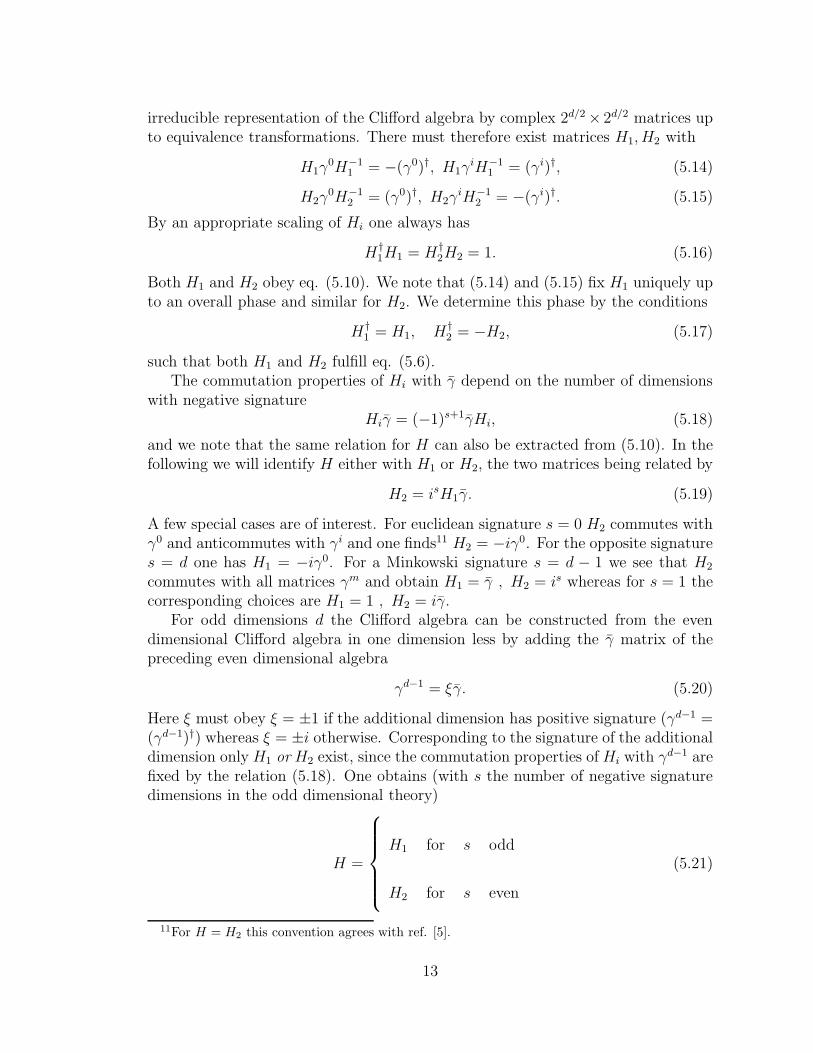
irreducible representation of the Clifford algebra by complex 2d/2× 2d/2 matrices upto equivalence transformations. There must therefore exist matrices H1, H2 with

H1γ0H−1

1 = −(γ0)†, H1γiH−1

1 = (γi)†, (5.14)

H2γ0H−1

2 = (γ0)†, H2γiH−1

2 = −(γi)†. (5.15)

By an appropriate scaling of Hi one always has

H†1H1 = H†

2H2 = 1. (5.16)

Both H1 and H2 obey eq. (5.10). We note that (5.14) and (5.15) fix H1 uniquely upto an overall phase and similar for H2. We determine this phase by the conditions

H†1 = H1, H†

2 = −H2, (5.17)

such that both H1 and H2 fulfill eq. (5.6).The commutation properties of Hi with γ depend on the number of dimensions

with negative signatureHiγ = (−1)s+1γHi, (5.18)

and we note that the same relation for H can also be extracted from (5.10). In thefollowing we will identify H either with H1 or H2, the two matrices being related by

H2 = isH1γ. (5.19)

A few special cases are of interest. For euclidean signature s = 0 H2 commutes withγ0 and anticommutes with γi and one finds11 H2 = −iγ0. For the opposite signatures = d one has H1 = −iγ0. For a Minkowski signature s = d − 1 we see that H2

commutes with all matrices γm and obtain H1 = γ , H2 = is whereas for s = 1 thecorresponding choices are H1 = 1 , H2 = iγ.

For odd dimensions d the Clifford algebra can be constructed from the evendimensional Clifford algebra in one dimension less by adding the γ matrix of thepreceding even dimensional algebra

γd−1 = ξγ. (5.20)

Here ξ must obey ξ = ±1 if the additional dimension has positive signature (γd−1 =(γd−1)†) whereas ξ = ±i otherwise. Corresponding to the signature of the additionaldimension only H1 or H2 exist, since the commutation properties ofHi with γ

d−1 arefixed by the relation (5.18). One obtains (with s the number of negative signaturedimensions in the odd dimensional theory)

H =

H1 for s odd

H2 for s even

(5.21)

11For H = H2 this convention agrees with ref. [5].

13

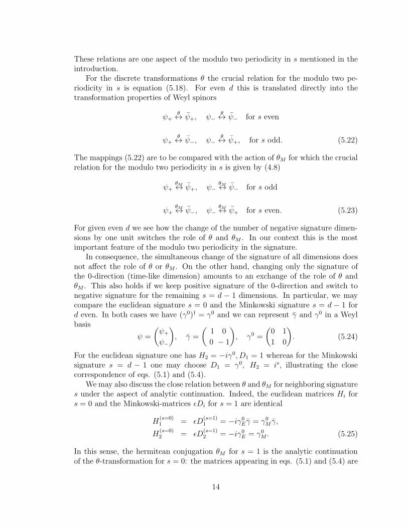
These relations are one aspect of the modulo two periodicity in s mentioned in theintroduction.

For the discrete transformations θ the crucial relation for the modulo two pe-riodicity in s is equation (5.18). For even d this is translated directly into thetransformation properties of Weyl spinors

ψ+θ↔ ψ+, ψ−

θ↔ ψ− for s even

ψ+θ↔ ψ−, ψ−

θ↔ ψ+, for s odd. (5.22)

The mappings (5.22) are to be compared with the action of θM for which the crucialrelation for the modulo two periodicity in s is given by (4.8)

ψ+θM↔ ψ+, ψ−

θM↔ ψ− for s odd

ψ+θM↔ ψ−, ψ−

θM↔ ψ+ for s even. (5.23)

For given even d we see how the change of the number of negative signature dimen-sions by one unit switches the role of θ and θM . In our context this is the mostimportant feature of the modulo two periodicity in the signature.

In consequence, the simultaneous change of the signature of all dimensions doesnot affect the role of θ or θM . On the other hand, changing only the signature ofthe 0-direction (time-like dimension) amounts to an exchange of the role of θ andθM . This also holds if we keep positive signature of the 0-direction and switch tonegative signature for the remaining s = d − 1 dimensions. In particular, we maycompare the euclidean signature s = 0 and the Minkowski signature s = d − 1 ford even. In both cases we have (γ0)† = γ0 and we can represent γ and γ0 in a Weylbasis

ψ =

(ψ+

ψ−

), γ =

(1 0

0 − 1

), γ0 =

(0 1

1 0

). (5.24)

For the euclidean signature one has H2 = −iγ0, D1 = 1 whereas for the Minkowskisignature s = d − 1 one may choose D1 = γ0, H2 = is, illustrating the closecorrespondence of eqs. (5.1) and (5.4).

We may also discuss the close relation between θ and θM for neighboring signatures under the aspect of analytic continuation. Indeed, the euclidean matrices Hi fors = 0 and the Minkowski-matrices ǫDi for s = 1 are identical

H(s=0)1 = ǫD

(s=1)1 = −iγ0E γ = γ0M γ,

H(s=0)2 = ǫD

(s=1)2 = −iγ0E = γ0M . (5.25)

In this sense, the hermitean conjugation θM for s = 1 is the analytic continuationof the θ-transformation for s = 0: the matrices appearing in eqs. (5.1) and (5.4) are

14

identical. The only modification is the additional flip of the zero momentum compo-nent q0 which is related to the additional minus sign under complex conjugation ofthe phase in the analytic continuation of the vielbein component e m

0 , as discussedin sect. 3.

Finally, we note that invariance under θ for a Minkowski signature s = 1 amountsto invariance under a time-reversal symmetry.

6 Generalized complex conjugation with euclidean

signature

Having established the close correspondence of θ for euclidean signature with θM forMinkowski signature suggests that θ can be used to define a new operation of gen-eralized complex conjugation within Grassmann algebras with euclidean signature.Our guiding principle is the observation that θM defines a complex conjugation inthe basis (ψ, ψ). If a similar complex conjugation based on θ is defined in the basis(ψ, ψ) for euclidean signature, this operation will induce similar mappings betweenWeyl spinors as θM for a Minkowski signature (cf. (5.22), (5.23)). With respect tothe new complex conjugation the Majorana spinors with euclidean signature shoulddirectly correspond to Majorana spinors with Minkowski signature. Also the posi-tivity properties related to hermiticity in Minkowski signature should carry over toeuclidean signature.

In a Fourier representation

ψ(x) =∑

q

exp(iqµxµ)ψ(q) , ψ(x) =

∑

q

exp(−iqµxµ)ψ(q) (6.1)

we define for euclidean Dirac spinors the generalized complex conjugation

ψ∗(q) = H∗ψ(θq),

ψ∗(q) = H−1ψ(θq). (6.2)

With our conventions H = −iγ0 for the signature s = 0 this relation is the same asin Minkowski space s = 1(4.12) up to a q0 reflection, θ(q0, ~q) = (−q0, ~q),

ψ∗(q) = i(γ0)∗ψ(θq),

ψ∗(q) = iγ0ψ(θq), (6.3)

or, in the usual “row representation” of ψ (ψT → ψ)

ψ(q) = −iψ†(θq)γ0. (6.4)

We can again define real and imaginary parts of ψ by the appropriate linear combi-nations

ψ(q) = ψR(q) + iψI(q),

ψ∗(q) = ψR(q)− iψI(q). (6.5)

15

This demonstrates again the complete analogy of spinor degrees of freedom in anMinkowski or euclidean formulation. Instead of ψ and ψ we can also take ψR andψI or ψ and ψ∗ as independent fermionic degrees of freedom. The new complexstructure does not necessitate a “doubling” of euclidean spinor degrees of freedom.

The compatibility of a (momentum-independent) linear transformation ψ → Aψwith the complex conjugation requires again that ψ∗ transforms according to ψ∗ →A∗ψ∗. This replaces eq. (4.7) by the requirement

ψ → ψH−1A†H. (6.6)

Despite the close similarity of the new complex conjugation (6.2) with the formula-tion for Minkowski signature we recall that the transformation properties of spinorsare originally formulated in terms of ψ and ψ. Not all transformations need to beconsistent with the complex structure. (This is similar to the example of 2M realscalar fields which can be combined into M complex fields. Among the possibleO(2M) symmetry transformations only the subgroup U(M) is compatible with thecomplex structure.) Compatibility with the complex structure holds trivially forvector-like global unitary transformations where U does not act on spinor indices.As a consequence of the modulo two periodicity discussed in the last section thechiral transformations are compatible with the complex structure only if we chooseθ for euclidean signature and θM for Minkowski signature.

The Lorentz transformations, in contrast, are only compatible with the com-plex structure θM and not with θ (cf. (5.10). For euclidean signature and complexconjugation θ the Lorentz transformations mix real and imaginary parts of ψ ina way which cannot be expressed in terms of multiplication with a complex ma-trix. These properties, together with the reflection of one coordinate, constitutethe main qualitative difference between possible complex structures for Minkowskior euclidean signature. Whereas for Minkowski signature the complex conjugationθM is compatible with both chiral and Lorentz transformations, the same cannot berealized for euclidean signature. For euclidean Dirac spinors we can, in principle,define the two different complex structures θ and θM . One is compatible with chiraltransformations (θ), the other with Lorentz transformations (θM ), but none withboth.

In practice, it is most convenient for euclidean spinors to define all transforma-tions for ψ and ψ. We will use the complex conjugation θ since only this is compatiblewith the chiral structure and related to the necessary positivity properties of thefermionic action. This choice also guarantees a close analogy between euclidean andMinkowski signature. We only have to remember that the Lorentz transformationsof ψ and ψ cannot be represented in the basis (ψR, ψI) by a multiplication of acomplex spinor ψ with a complex matrix. One rather needs the transformationsof both ψ and ψ and can then infer the appropriate transformations of ψR and ψIusing ψR(q) =

12(ψ(q) + iγ0ψ(θq)), ψI(q) = − i

2(ψR(q)− iγ0ψ(θq)).

16

7 “Real” fermionic actions

A fermionic action Sψ which is invariant under either one of the transformationsθM or θ will be called real. This can be generalized to other involutions whichinvolve a complex conjugation. We will collectively denote such transformations byθ. In this section we establish for a euclidean signature that the fermionic functionalintegration (2.7) with a real fermionic action gives a real result, provided Sψ containsonly terms with an even number of Grassmann variables. The partition functionZ is then real. The reality properties for Minkowski signature follow by analyticcontinuation.

The mere existence of the involution θ which maps ψ onto ψ requires that thefields ψ and ψ come in associated pairs (ψu, θψu) = (ψu, Euvψv). (Note that θ2 = 1forbids θψu = 0.) Using detE = 1 one can always write the functional measure inthe form used in (2.3) and establish its invariance under θ

∫DψDψ ≡

∫ ∏

u′

(dψu′dψu′) =

∫ ∏

u′

(dψu′d(θψu′))

=

∫ ∏

u′

(d(θψ)u′d(θψ)u′) =

∫ ∏

u′

((dθψ)u′d(θψ)u′). (7.1)

We assume here and in the following that the number of degrees of freedom ψu iseven. Then detH = ±1 or det ǫD = ±1 implies detE = 1.

Real euclidean action

First we consider a euclidean quadratic fermionic action

SE = ψuAuvψv. (7.2)

Invariance under θ requires θ(A) = A according to

θ(SE) = (θψ)vA∗uv(θψ)u = ψu(θ(A))uvψv = SE . (7.3)

For the transformations θM and θ one has

θM (A) = D†A†D−1,

θ(A) = SH†A†H−1S, (7.4)

where S operates a time reflection, i.e. S(ψ(q)) = ψ(θ(q)), S2 = 1. In consequence,the functional integration (2.3) yields a real result if SE is θ invariant

det(θ(A)) = detA† = (detA)∗ = detA. (7.5)

(We employ here the fact that for any variable ψ(q) there is a variable ψ(θ(q))such that the number of variables ψu is even and therefore det(H†H−1) =1, detD†D−1 = 1. The partition function Z = det(−A) = detA (2.7) is there-fore real.

17

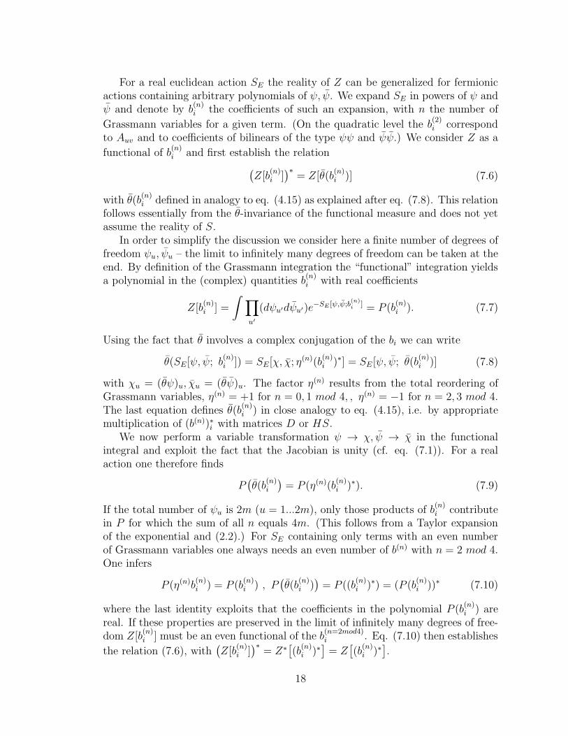
For a real euclidean action SE the reality of Z can be generalized for fermionicactions containing arbitrary polynomials of ψ, ψ. We expand SE in powers of ψ andψ and denote by b

(n)i the coefficients of such an expansion, with n the number of

Grassmann variables for a given term. (On the quadratic level the b(2)i correspond

to Auv and to coefficients of bilinears of the type ψψ and ψψ.) We consider Z as a

functional of b(n)i and first establish the relation

(Z[b

(n)i ])∗

= Z[θ(b(n)i )] (7.6)

with θ(b(n)i defined in analogy to eq. (4.15) as explained after eq. (7.8). This relation

follows essentially from the θ-invariance of the functional measure and does not yetassume the reality of S.

In order to simplify the discussion we consider here a finite number of degrees offreedom ψu, ψu – the limit to infinitely many degrees of freedom can be taken at theend. By definition of the Grassmann integration the “functional” integration yieldsa polynomial in the (complex) quantities b

(n)i with real coefficients

Z[b(n)i ] =

∫ ∏

u′

(dψu′dψu′)e−SE [ψ,ψ;b

(n)i ] = P (b

(n)i ). (7.7)

Using the fact that θ involves a complex conjugation of the bi we can write

θ(SE[ψ, ψ; b(n)i ]) = SE[χ, χ; η

(n)(b(n)i )∗] = SE [ψ, ψ; θ(b

(n)i )] (7.8)

with χu = (θψ)u, χu = (θψ)u. The factor η(n) results from the total reordering ofGrassmann variables, η(n) = +1 for n = 0, 1 mod 4, , η(n) = −1 for n = 2, 3 mod 4.The last equation defines θ(b

(n)i ) in close analogy to eq. (4.15), i.e. by appropriate

multiplication of (b(n))∗i with matrices D or HS.We now perform a variable transformation ψ → χ, ψ → χ in the functional

integral and exploit the fact that the Jacobian is unity (cf. eq. (7.1)). For a realaction one therefore finds

P(θ(b

(n)i

)= P (η(n)(b

(n)i )∗). (7.9)

If the total number of ψu is 2m (u = 1...2m), only those products of b(n)i contribute

in P for which the sum of all n equals 4m. (This follows from a Taylor expansionof the exponential and (2.2).) For SE containing only terms with an even numberof Grassmann variables one always needs an even number of b(n) with n = 2 mod 4.One infers

P (η(n)b(n)i ) = P (b

(n)i ) , P

(θ(b

(n)i ))= P ((b

(n)i )∗) = (P (b

(n)i ))∗ (7.10)

where the last identity exploits that the coefficients in the polynomial P (b(n)i ) are

real. If these properties are preserved in the limit of infinitely many degrees of free-dom Z[b

(n)i ] must be an even functional of the b

(n=2mod4)i . Eq. (7.10) then establishes

the relation (7.6), with(Z[b

(n)i ])∗

= Z∗[(b

(n)i )∗

]= Z

[(b

(n)i )∗

].

18

In absence of other fields a real fermionic action requires θ(b(n)i ) = b

(n)i . The

relation (7.6) then directly implies that the functional integral over a real SE withonly even numbers of ψ or ψ is real

Z =

∫DψDψ exp(−SE) = Z∗. (7.11)

Typical fermionic actions only involve even numbers of fermions – for example, this isa necessary requirement for Lorentz-invariance. Osterwalder-Schrader positivity foreuclidean fermions implies then immediately the reality12 of the fermionic functionalintegral. We note that we have not assumed continuity of space-time such that thisobservation applies directly to lattice theories.

It is easy to show that the expectation values of all θ-even operators are realwhereas the ones for θ-odd operators are purely imaginary. (We assume that theoperators involve an even number of Grassman variables.) Let us denote the evenand odd operators by Ok

R and OlI , θ(OR) = OR, θ(Oi) = −OI . One concludes (with

real fk, fl)

〈fkOkR + iflO

lI〉 = Z−1

∫DψDψ(fkO

kR + iflO

lI) exp(−SE)

= 〈fkOkR + iflO

lI〉

∗ (7.12)

since we may consider −ln(fkOkR + iflO

lI) as an additional part of a real fermionic

action. By suitable linear combinations one finds for an arbitrary operator

〈θ(O)〉 = 〈O〉∗. (7.13)

Fermions and bosons

We can extend our discussion to the case where the b(n)i depend on additional

bosonic fields φ. If the bosonic fields also transform under θ we have to replace ineq. (7.8) (b

(n)i )∗ by b

(n)i = b

(n)∗i

(θ(φ)

)and correspondingly generalize the meaning of

θ(b(n)i ). Repeating the discussion above yields

Z[θ(b(n)i (φ)

)]= Z

[(b(n)i

)∗(θ(φ)

)]= Z∗

[(b(n)i

)∗(θ(φ)

)]. (7.14)

Typically, for the euclidean reflection θ the transformation of a scalar field withpositive θ-parity also involves a reflection of the time coordinate θ

(φ(x)

)= φ∗(θx).

12We observe that functional integration over fermionic actions with even and odd numbers offermions would not give a real result even in case of a real action. For a given m one may replace,for example, three terms with two fermions ((η(2))3 = −1) by two terms with three fermions((η(3))2 = 1) such that P would necessarily have an imaginary part. Our discussion does not cover

the case that the b(n)i are Grassmann variables themselves as, for example, linear source terms. A

generalization to this case is straightforward.

19

(In this case a Yukawa coupling b(2)(φ) = hφ(x) implies(b(2))∗(

θ(φ))≡ h∗φ∗

(θ(x)

).)

A real action obeys again θ(b(n)i (φ)

)= b

(n)i (φ) and therefore

Z∗[θ(φ)

]= Z[φ]. (7.15)

This can be used directly for establishing the reality properties of the effectivebosonic action Seff [φ] which obtains by integrating out the fermionic fields

Z[φ] = exp(−Seff [φ]) =

∫DψDψ exp(−S[φ, ψ, ψ]), (7.16)

namelyS∗eff [θ(φ)]) = Seff [φ] (7.17)

where the star for S∗eff means complex conjugation of all couplings. In general,

the fermionic functional integral with a real action can lead to an imaginary part ifθ(φ) 6= φ∗,

Im exp(−Seff [φ]) = −i

2exp

(− Seff [φ]

)− exp

(− S∗

eff [φ∗])

= −i

2exp(−Seff [φ])− exp(−Seff [(θ(φ))

∗]. (7.18)

As an example we may consider euclidean signature with a real scalar field obey-ing θ

(φ(x)

)= φ(θx). According to eq. (7.17) a possible local term in the effective

action with an odd number of time derivatives must have an imaginary coefficient.An example for such a local term is (α real).

Seff = iα

∫

x

ǫµνρσ∂µφ∂νφ∂ρφ∂σφ+ . . . (7.19)

We may also evaluate Z[φ] for a given time odd scalar field configuration φ(θx) =−φ(x), with

ImZ[φ] = −i

2

(Z[φ]− Z[−φ]

). (7.20)

The imaginary part of Z[φ] does not vanish if Seff [φ] contains terms that are oddin φ.

Real expectation values

Often one is interested in the expectation value of some operator

< O[φ, ψ, ψ] >=

∫DφDψDψO[φ, ψ, ψ] exp(−S[φ, ψ, ψ]) (7.21)

Let us assume that the functional measure∫Dφ is invariant under θ in the sense

that it can be written in the form∏∫

dφd(θ(φ)). For real S one concludes

< θ(O[φ, ψ, ψ]) >=< O[φ, ψ, ψ] > (7.22)

20

such that the expectation values of all θ-odd operators vanish. For the case θ(φ) = φ∗

the imaginary part of the fermionic integration vanishes and the remaining bosonicintegral is real, implying < O >=< O >∗. This situation is typically realized forθ ≡ θM . On the other hand, for an euclidean signature the action may only beinvariant under θ and not under θM . Then the time reflection implies θ(φ) 6= φ∗. Inthis case we further assume that the bosonic functional measure can be written asa product

∏∫dφd(θ(φ))∗. We distinguish between real operators obeying

OR[φ, ψ, ψ] = θOR[φ∗, ψ, ψ] (7.23)

and imaginary operators for which (7.23) involves a minus sign. From θ(φ∗) =(θ(φ))∗ and (7.17) one concludes

< θO[φ∗, ψ, ψ] >=< O[φ, ψ, ψ] >∗ (7.24)

Real operators have therefore always real expectation values, whereas the expec-tation values of imaginary operators are purely imaginary. For real operators theimaginary parts (7.18) of the contributions to the functional integral from φ and(θ(φ))∗ exactly cancel. They can therefore simply be omitted and one can replaceexp(−Seff ) by its real part.

These properties have implications for euclidean lattice simulations of gaugetheories with fermions. For a computer simulation the fermionic functional integralhas to be performed analytically and the result is in general not real. As long asonly the expectation values of real operators are computed, one can simply omit theimaginary parts of the fermionic integration and work with a real effective actiondefined by

exp(−Seff [φ]) = Re exp(−Seff [φ]) =1

2exp(−Seff [φ]) + exp(−Seff [(θ(φ))

∗])

(7.25)The result remains exact.

Bosonization

Finally we notice that the positivity properties should be respected if one (par-tially) bosonizes a fermionic theory. Bosonization typically replaces a fermion bilin-ear by a bosonic field. Let us consider an euclidean signature with fermion bilinearsrepresented by Lorentz scalars φ. If one wants to represent the action of θ on φby standard complex conjugation θ(φ(x)) = φ∗(θx), one has to make sure thatφ(x) + φ∗(θx) corresponds to a real fermionic bilinear operator. For d even and a, binternal indices for different fermion species, the real scalar bilinears are

ψa−(x)ψb+(x)− ψb+(θx)ψ

a−(θx) , i(ψa−(x)ψ

b+(x) + ψb+(θx)ψ

a−(θx)) (7.26)

We emphasize that ψψ is an imaginary operator whereas ψγψ is real. Operators ofthe type ψaψb, ψaγψb have no definite reality property for a 6= b. Corresponding to(7.26) one may bosonize the bilinear ψa−(x)ψ

b+(x) by a complex scalar field φab(x).

21

The complex conjugated field (φab(x))∗ corresponds then to −ψb+(x)ψa−(x), whereas

ψa+(x)ψb−(x) is replaced by −(φ†)ab(x). The bilinears iψa(x)ψb(x) and ψa(x)γψb(x)

transmute into hermitean scalar fields.

Reality for Minkowski signature

Formally, a real quadratic Minkowski action SM is also sufficient to guaranteea real partition function Z =

∫exp(iSM). For SM = ψuA

Muvψv we now have the

relation

Z = det(iAM) = det(iθ(AM)

)= det

(i(AM)†

)=(det(−iAM )

)∗=(det(iAM )

)∗.

(7.27)For the last relation we use once more the property that the number of spinors ψuis even. Again, Z∗ = Z. Furthermore, if the number of spinors ψu is 4 mod 4 onemay use det(−iAM ) = det(AM). This formal reality of Z does not remain valid,however, in the presence of the poles characteristic for the momentum integrals withMinkowski signature. In this case it is destroyed by the non-hermitean regulatorterms that have to be added to SM in order to make the momentum integrals welldefined. As a result, the momentum integrals appearing in the computation of lnZproduce a factor i such that the fluctuation contribution to −i lnZ is real, just asthe classical part, −i lnZcl = SM [ψ = 0].

As an example, we investigate a Yukawa coupling between spinors and a complexscalar field φ for d = 4

− SM =

∫

x

iψγµ∂µψ + h(ψRφψL − ψLφ∗ψR). (7.28)

With real h and θM(φ) = φ∗ the action is real with respect to θM , θM(SM) = S†M =

SM . Performing the Gaussian integral for the fermions yields formally for constantφ, with q

/= γµqµ,

lnZ[φ] = tr

∫d4q

(2π)4ln

(− q/+hφ

1 + γ

2− hφ∗1− γ

2

). (7.29)

We are interested in the φ dependence of lnZ (Ω4: four volume, ρ = φ∗φ)

1

Ω4

∂2 lnZ

∂φ∂φ∗= 2h2

∫

q

q2

(q2 + h2ρ)2= µ2(ρ). (7.30)

In order to avoid discussing the complications of the UV-regularization we considerhere the UV-finite derivative

∂2µ2

∂ρ2= 12h6

∫

q

q2

(q2 + h2ρ)4=

i

48π2h2ρ. (7.31)

Even though the q− integral is formally real the momentum integration is welldefined only by adding to q2 a small imaginary part, q2 → q2 − iǫ, ǫ > 0. The poles

22

at q0 = ±√~q2 + h2ρ− iǫ are now away from the real axis and the integration yields

an imaginary result. This demonstrates that the formally real expression ln detAMturns actually out to be imaginary.

More generally, we expect that functional integration over fermions with a realMinkowski-action SM yields a real effective action13

SM,eff [φ] = −i lnZ[φ]. (7.32)

and therefore purely imaginary lnZ. Indeed, if the Minkowski-action SM obtainsfrom the euclidean action SE by analytic continuation (−iSM = SE (anal. contd.))we may exploit analyticity also for the effective action. As demonstrated above, aθ-invariant SE yields a real effective action Seff . By analytic continuation one infersthat SM is θM -invariant. Also the analytic continuation of Seff yields −iSM,eff . Inturn, SM,eff should now be real with respect to θM (hermitean conjugation).

8 Hermitean spinor bilinears

Let us now concentrate on hermitean spinor bilinears. In particular, from hermiteanbilinears containing both ψ and ψ one can easily construct real fermionic actionsobeying θ(A) = A in eq. (7.2). For θM and D = D1 the action of θM reorders theγ-matrices according to

θM (ψ(q)γmγn...γpψ(q)) = ψ(q)γp...γnγmψ(q). (8.1)

For even dimensions one also may use

θM (ψ(q)γmγn...γpγψ(q)) = (−1)s+Qψ(q)γp...γnγmγψ(q) (8.2)

with Q the total number of matrices γm. For D = D1 the invariants with respect toθM can then be constructed by multiplying the following terms with real coefficients14

ψψ , isψγψ , ψγmψ , is−1ψγmγψ , iψΣmnψ , is−1ψΣmnγψ. (8.3)

If, instead, we use D = D2 the hermitean (θM -invariant) bilinears are

iψψ , is−1ψγψ , ψγmψ , is−1ψγmγψ , ψΣmnψ , isψΣmnγψ. (8.4)

In consequence, the kinetic term (2.15) is invariant under θM for both D1 and D2.The corresponding bilinear transformation rules for θ are given by

θ(ψ(q)γmγn...γpψ(q)) = κψ(θq)γp...γnγmψ(θq)

θ(ψ(q)γmγn...γpγψ(q)) = (−1)s+1+Qκψ(θq)γp...γnγmγψ(θq) (8.5)

13Strictly speaking, this holds provided we choose a regularization which is consistent with thisproperty.

14The kinetic term reads −∫

ddq

(2π)d ψ(q)qµγµψ(q).

23

withγ0 = −γ0, γi = γi for i 6= 0 (8.6)

and

κ =

1 forH = H1

(−1)Q+1 forH = H2

(8.7)

For H = H2 one finds among the possible θ-invariants with real coefficients cj(with γi, i 6= 0)

SE =

∫ddq

(2π)dψ(q)(cjOj)ψ(q)

Oj = i , isγ , iγ0 , γi , qµγµ , is+1γ0γ , isγiγ , ... (8.8)

As it should be the list (8.4) of θM -invariants for s = 1 , D = D2 correspondsprecisely15 to the θ-invariants (8.8) for s = 0 , H = H2, reflecting analytic con-tinuation. For irreducible Weyl, Majorana or Majorana-Weyl spinors some of thebilinears vanish identically. This is discussed in detail in ref. [1], where tables ofallowed and forbidden bilinears, in particular mass terms, can be found.

For euclidean spinors with Osterwalder-Schrader positivity a fermion mass termin our convention (H = H2) is either imψψ or mψγψ. It is also worth mentioningthat the euclidean fermion number operator is given by

Nψ = i

∫dd−1q

(2π)d−1ψ(q)γ0ψ(q) =

∫dd−1q

(2π)d−1ψ†(q)ψ(q) (8.9)

(cf. eq. (6.4)). Invariance of Nψ with respect to θ guarantees that the fermionicfunctional integral results in a real determinant even in presence of a nonvanishingchemical potential associated to Nψ.

9 Generalized charge conjugation

The properties of the discrete symmetries charge conjugation, parity reflection andtime reversal depend on the dimension and the generalized signature. We call ageneralized euclidean signature (E) the case where θ = θ is used to define a real ac-tion. For d even (E) corresponds to s even. Conversely, for a generalized Minkowskisignature (M) one uses θ = θM for the definition of “reality” – for d even thiscorresponds to s odd.

Since ψu and ψv are independent Grassmann variables the spinors ψ(x) andψ(x) correspond in a formal group theoretical sense to two distinct Dirac spinors.If we define a combined spinor ψ(x) =

(ψ(x), ψ(x)

)this will always be a reducible

representation of the Lorentz group, with 2[d2 ]+1 components. We therefore expect

15This correspondence holds modulo a factor factor i for each γ0 factor in the θ-invariants

24

that in the group theoretical sense there always exists a generalized Majorana-typeconstraint which can reduce ψ to a single Dirac spinor. This extends to Weyl spinorsif we define ψ+ = (ψ+, ψ±) with a choice of ψ± such that ψ± contains to equivalentWeyl spinors. We can define generalized Majorana- and Majorana-Weyl spinors inthis way in a group theoretical sense.

To what extent these representations of the Lorentz group can be used for a de-scription of physical particles will depend on the possible existence of a kinetic termin the action. This will not be realized for all generalized Majorana and Majorana-Weyl spinors. We will see in sect. 10 that for euclidean signature (E) physicalMajorana spinors exist for d = 2, 3, 4, 8, 9 mod 8, and Majorana-Weyl spinors ford = 2 mod 8. These are precisely the dimensions for which Majorana and Majorana-Weyl spinors exist for Minkowski signature [1]. They differ from the dimensions forwhich euclidean Majorana and Majorana-Weyl spinors exist in a group theoreticalsense [1]. We also emphasize that the compatibility of the Majorana constraint withcomplex conjugation depends on the choice of the involution θ, typically θM for (M)and θ for (E).

A generalized charge conjugation CW is a map from ψ to ψ which commutes withthe Lorentz transformations. Expressed in the basis ψ, ψ it is purely a map in thespace of spinors. In contrast to the transformations θ or θ it does not involve anadditional complex conjugation of the coefficients in the Grassmann algebra. ThusCW constitutes a symmetry if the action is invariant. It is convenient to representCW by a matrix acting on ψ(x)

CW

(ψ(x)

ψ(x)

)=

(0 W1

W2 0

)(ψ(x)

ψ(x)

). (9.1)

Corresponding to the convention (6.1), CW involves an additional reflection in mo-mentum space, i.e. ψ(q) → W1ψ(−q). In momentum space the combined spinor istherefore defined as ψ(q) =

(ψ(q), ψ(−q)

). Commutation with the Lorentz trans-

formations,

[CW , Σ] = 0 , Σ = −1

2ǫmn

(Σmn 0

0 − (Σmn)T

)(9.2)

requiresW−1

1 ΣmnW1 = W2ΣmnW−1

2 = −(Σmn)T . (9.3)

Furthermore, invariance of the fermion kinetic term −Σqψ(q)γµqµψ(q) necessi-

tatesW T

2 γmW1 = (γm)T . (9.4)

We emphasize that a generalized charge conjugation can be defined without thecondition (9.4). The latter should be viewed as a condition for a dynamical theoryof fermions of the standard type. We concentrate here on the case C2

W = ǫ = ±1where

W1 = (CT )−1, W2 = ǫCT (9.5)

25

andCTΣmn(CT )−1 = −(Σmn)T , (9.6)

such that eq. (9.4) results in the condition

Cγm(CT )−1 = ǫ(γm)T . (9.7)

We omit the possible alternative for even dimensions where C2W = ±γ.

A simultaneous solution of the conditions (9.3) and (9.4) obtains for

CT = δC, δ2 = 1,

CγmC−1 = ǫδ(γm)T ,

CΣmnC−1 = −(Σmn)T . (9.8)

We use the labels [1] C = C1, δ = δ1 for ǫδ = −1 and C = C2, δ = δ2 for ǫδ = 1,with C2 = C1γ for d even. For even d there is an alternative possibility to fulfill eq.(9.6)

iCT γγm(CT )−1 = ǫδ(γm)T (9.9)

and eq. (9.7) follows from

C = iδCT γ , δ2 = 1. (9.10)

In this case we use C = C1, δ = δ1 for ǫδ = −1 and C = C2, δ = δ2 for ǫδ = 1.For d even the existence of the matrices C1, C2, C1, C2 obeying eqs. (9.6), (9.9) isguaranteed by the fact that (γm)T ,−(γm)T , γm and iγγm all obey the same definingrelations for the Clifford algebra γm, γn = 2ηmn. The values δ1,2 depend on thenumber of dimensions [6], [7], [1]

δ1 =

1 for d = 6, 7, 8 mod 8

−1 for d = 2, 3, 4 mod 8

δ2 =

1 for d = 2, 8, 9 mod 8

−1 for d = 4, 5, 6 mod 8

(9.11)

In even dimensions one finds from (9.6)

γT = (−1)d2CT γ(CT )−1. (9.12)

26

In order to understand the action of CW on Weyl spinors we first introduce a matrix

Γ =

γ 0

0 (−1)d/2γT

. (9.13)

The eigenvectors to the eigenvalues ±1 correspond to the two inequivalent spinorrepresentations. By the convention (2.16) we always have for blockdiagonal γ

ψ =

(ψ+

ψ−

), ψ =

(ψ−

ψ+

), (9.14)

and we recall that ψ− is in a representation equivalent to ψ+ for d = 4mod 4 whereasψ+ and ψ+ are equivalent for d = 2 mod 4. From eq. (9.12) one concludes

[CW , Γ] = 0. (9.15)

The generalized charge conjugation maps equivalent spinor representations in ψand ψ into each other. The matrix Γ is, however, not compatible with every complexstructure. We demonstrate this for the complex structure θM and introduce

ˆγ =

(γ 0

0 DT γD∗

)=

(γ 0

0 − γT

)(9.16)

For d = 2 mod 4 one observes compatibility with the complex structure Γ = ˆγ,whereas for d = 4 mod 4 the mapping ψ → Γψ cannot be expressed by the rulesψ → γψ, ψ = ǫDTψ∗ → ǫDT (γψ)∗ which rather correspond to ψ → ˆγψ. For thetransformation ψ → ˆγψ one finds

[CW , ˆγ] = 0 for d = 2 mod 4

CW , ˆγ = 0 for d = 4 mod 4. (9.17)

We emphasize that for the generalized charge conjugation the properties (9.12)-(9.17) depend only on the dimension and not on the signature (as for the algebraiccharge conjugation C discussed in [1]). This is related to the fact that the definitionof CW is based on mappings between ψ and ψ and therefore involves the properties ofspinor representations under transposition16, which are independent of the signature.This setting guarantees a close analogy between Minkowski and euclidean signature.

For the second solution (9.9) in even dimensions one finds

γT = −CγC−1 = −CT γ(CT )−1 = (−1)d/2CT γ(CT )−1 (9.18)

One concludes that this solution is possible only for d = 2 mod 4 where [CW , ˆγ] = 0.

16The algebraic charge conjugation C [1] is based on a mapping ψ → ψ∗ and therefore involvesthe properties of representations under complex conjugation which depend on the signature.

27

10 Generalized Majorana spinors

Generalized Majorana-type spinors correspond to an identification of ψ(x) and±CW (ψ(x)). Furthermore, 1

2(1± CW ) must be projectors or C2

W = 1. Then, for

C2W = 1 , ǫ = 1, (10.1)

generalized Majorana spinors are defined by

ψW± =1

2(1± CW )ψ, ψ =

(ψ

ψ

). (10.2)

Furthermore, since CW commutes with Γ, one can have generalized Majorana-Weylspinors which are both eigenstates of CW and Γ. We observe that the commutationof CW with the Lorentz transformations (9.6) gives no restriction on ǫ. In a group-theoretical sense we can therefore define generalized Majorana-Weyl spinors in alleven dimensions. They correspond to the irreducible spinor representations of theLorentz group.

The requirement of invariance of the spinor kinetic term changes the picture.The value of ǫ depends on δ and therefore only on the dimension and not on thesignature. From the condition

ǫ = −δ1 = δ2 (10.3)

and (9.11) we infer that an invariant kinetic term for Majorana spinors is not possiblefor all dimensions. Therefore “physical” generalized Majorana spinors are possibleonly for d = 2, 3, 4, 8, 9 mod 8. Physical generalized Majorana-Weyl spinors existfor d = 2 mod 8.

For the solution (9.8), d = 2, 3, 4.8, 9 mod 8, and Minkowski signature the gen-eralized Majorana spinors ψW correspond to the standard formulation of Majoranaspinors as real representations of the Lorentz group [1]. This is not the case anymorefor euclidean signature. Indeed, for d = 4 the euclidean rotation group SO(4) hasno real representations. A definition of Majorana spinors as real representations im-plies that four euclidean dimensions do not admit Majorana spinors [1]. This puzzleis solved by the observation that the appropriate notion of complex conjugation foreuclidean signature involves a time reflection. Using the definitions of sect. 9 thecharge conjugate spinor obeys

ψc(x) = CW (ψ(x)) = (CT )−1ψ(x) = B−1W ψ∗(θx),

ψc(x) = CW (ψ(x)) = ǫCTψ(x), (10.4)

with θx = x (M) or θx = θx (E) and

BW = B = CD−1 (M),

BW = −HCT (E). (10.5)

28

The matrix B obeys the relations

(Σmn)∗ = BΣmnB−1,

(γm)∗ =

−BγmB−1 for C = C1

BγmB−1 for C = C2

(10.6)

andB†B = 1, B∗B = ǫ. (10.7)

For a signature of the type (M) the charge conjugate spinor ψc coincides with thedefinition17 in [1]. In terms of complex conjugate spinors ψ∗ the euclidean Majorana-type spinor ψW is a non-local superposition

ψW+(x) =1

2ψ(x)− (HCT )−1ψ∗(θx). (10.8)

This should not obscure the property that in terms of the basic spinor fields ψ(x)and ψ(x) the generalized euclidean Majorana spinor is a perfectly local object

ΨW±(x) =1

2ψ(x)± (CT )−1ψ(x). (10.9)

The action of the generalized charge conjugation is perhaps most apparent in abasis

ψs =

(1 0

0 (CT )−1

)ψ =

(ψ

(CT )−1ψ

), (10.10)

where the Lorentz transformations are represented by a diagonal matrix (Σ =−1

2ǫmnΣ

mn)

Σs =

(1 0

0 (CT )−1

)Σ

(1 0

0 CT

)=

(Σ 0

0 Σ

). (10.11)

It simply reads

CW (ψs(x)) =

(0 1

ǫ 0

)ψs(x), (10.12)

such that for ǫ = 1 the upper and lower components of ψs are exchanged. For deven ˆγ and Γ take the form

ˆγs =

(1 0

0 (CT )−1

)(γ 0

0 − γT

)(1 0

0 CT

)=

(γ 0

0 τ γ

), Γs =

(γ 0

0 γ

), (10.13)

with τ = (−1)d2−1. Since ψ and ψ always contain equivalent Lorentz representations,

ψs is a reducible representation which is decomposed into irreducible representations

17In the notation of [1] one has B = B1 for C = C1 whereas for C = C2 one uses B = ±B2,with B = (−1)sB2 for even d. Correspondingly, ǫ is identified with ǫ1 or ǫ2.

29

by suitable projectors 12(1±CW ) (and 1

2(1± Γ) for d even). From a group-theoretical

point of view it is obvious that one can always define the transformation (10.12)with ǫ = 1 and perform the decomposition.

One still has to answer the question if a non-vanishing kinetic term exists for onlyone irreducible representation of the Lorentz group. This requires that a Lorentzvector is contained in the symmetric product of two identical irreducible spinor rep-resentations, and is the case for d = 2, 3, 9 mod 8. For these dimensions invariantactions involving a single irreducible generalized Majorana spinor (d = 3, 9 mod 8)or a irreducible generalized Majorana-Weyl spinor (d = 2 mod 8) can be formulated.For d = 4 mod 8 the kinetic term involves two inequivalent spinor representationsof the Lorentz group. One can still use generalized Majorana-Weyl spinors, but nota single one. The minimal setting for an invariant kinetic term consists of two in-equivalent generalized Majorana-Weyl spinors, which can be combined into one Weylspinor or one generalized Majorana spinor. Similarly, for d = 5, 6, 7 mod 8 the vec-tor is in the antisymmetric product of two equivalent irreducible spinors. A kineticterm therefore requires at least two generalized Majorana spinors, corresponding toa Dirac spinor for d = 5, 7 mod 8 or a Weyl spinor for d = 6 mod 8.

In conclusion, the algebraic notion of Majorana spinors is based on the transfor-mation properties of Lorentz representations under complex conjugation accordingto a classification into real, pseudoreal or complex representations. This classifica-tion depends on the signature [1]. The generalized Majorana spinors are related tothe decomposition of ψ+ψ into irreducible Lorentz representations. This is indepen-dent of the signature, and only distinguishes between d even or odd. The existence ofphysical generalized Majorana spinors is related to the decomposition of a symmet-ric product of two irreducible representations. This depends on the dimension, butnot on the signature. The notion of physical Majorana spinors is therefore compat-ible with analytic continuation in arbitrary dimension d. For Minkowski signature,the algebraic notion coincides with the physical Majorana spinors. For euclideansignature, algebraic and physical Majorana spinors differ: the physical Majoranaspinors do not coincide with real representations of SO(d). They correspond to asingle spinor representation, where the spinors ψ are given by appropriate linearcombinations of ψγ , rather than being independent variables.

11 Parity and time reversal

The Lorentz transformations contain the reflections of an even number of coordinateswith equal signature. Possible additional discrete symmetries involve a reflection ofan odd number of coordinates. We first consider parity in even dimensions witheuclidean (s = 0) or Minkowski (s = 1) signature. It involves the reflection ofd − 1 coordinates xi, i = 1...d − 1, whereas x0 remains unchanged (with η00 = −1for Minkowski signature). We work here in a fixed coordinate system, where thereflections act only on the spinor fields. On Dirac spinors a parity transformation

30

can be defined as

P1(ψ(q)) = ηPγ0ψ(P (q)),

P1(ψ(q)) = ηP (γ0)T ψ(P (q)), (11.1)

with P (q0) = q0, P (qi) = −qi. Invariance of the kinetic term requires

ηP ηPη00 = 1. (11.2)

For s = 0, 1 this implies ηP = (−1)s/ηP .Using the connection (4.1) between ψ and ψ∗ one finds for a Minkowski signature

(s = 1)P1ψ

∗(x) = ηPD∗(γ0)DTψ∗

(P (x)

)= σηP (γ

0)∗ψ∗(P (x)

), (11.3)

with σ = +1 for D = D1 and σ = −1 for D = D2. Compatibility of P1 with thecomplex structure requires

P1ψ∗(x) =

(P1ψ(x)

)∗= η∗P (γ

0)∗ψ∗(P (x)

)(11.4)

and thereforeηP = ση∗P . (11.5)

Combining with eq. (11.2) this yields

η∗PηP = ση00. (11.6)

For s = 1 the compatibility of the parity transformation (11.1) with the complexstructure requires the choice D = D2 such that σ = −1, ση00 = 1. For a euclideansignature (s = 0) we use the same parity transformation as for s = 1 in order

to remain compatible with analytic continuation, i.e. η(E)P γ0E = η

(M)P γ0M or η

(E)P =

−iη(M)P , η

(E)P = −iη

(M)P .

Let us now concentrate on D = D2, η∗PηP = 1, ηP = (−1)sη∗P . We still remain

with the freedom of a phase in ηP . In order to fix ηP , we first impose P 21ψ = ±ψ

or η2P = η2P = ±1. Next we require that the parity reflection commutes with thegeneralized charge conjugation CW ,

[CW , P1] = 0. (11.7)

This allows us to define the action of parity also for generalized Majorana spinors.Using (9.8) this yields

η2P = ǫδη00. (11.8)

In particular, for d = 4, s = 1, C = C1 (or ǫδ = −1) one finds ηP = −ηP =±1, P 2

1ψ = −ψ. For euclidean signature C = C1 implies an imaginary phase

ηP = −ηP = ±i, P 21ψ = −ψ. We choose η

(M)P = 1, η

(M)P = −1, η

(E)P = −i, η

(E)P = i.

31

The transformation of the fermion bilinears involving ψ and ψ is independent of thephase ηP and independent of the signature:

P1 : ψ+iγµ∂µψ+ ↔ ψ−iγ

µ∂µψ− , ψa+ψb− ↔ ψa−ψ

b+,

ψψ → ψψ , ψγψ → −ψγψ. (11.9)

In even dimensions there is an alternative version of the parity transformationinvolving γ

P2

(ψ(q)

)= ηPγ

0γψ(P (q)

),

P2

(ψ(q)

)= −ηPγ

0T γT ψ(P (q)

). (11.10)

The transformations P2 and P1 are related by a chiral transformation P2 = P1R−

where R− changes the sign of ψ− and ψ− while ψ+, ψ+ are invariant. The relations(11.2) and (11.5) also hold for P2. We conclude that for s = 1 only the complexstructure built on the choice D = D2 is compatible with the parity transformation.With respect to P2 the transformation properties of spinor bilinears are

P2 : ψ+iγµ∂µψ+ ↔ ψ−iγ

µ∂µψ− , ψa+ψb− ↔ −ψa−ψ

b+

ψψ → −ψψ , ψγψ → ψγψ. (11.11)

Since for s = 1, D = D2 the bilinear ψγψ is real (cf. eq. (8.4)) it seems naturalto use the parity transformation P2. In this case a mass term mψγψ with real mconserves parity.

For an odd number of dimensions the parity reflection of d − 1 coordinates iscontained in the continuous Lorentz transformations and needs not to be discussedseparately. There still exist non-trivial reflections of an odd number of space coor-dinates.

Generalized time reversal TW is a reflection of the remaining 0-component ofthe coordinates. This transformation also maps ψ into ψ and vice versa. In evendimensions one has18

TW (ψ(q)) = ηTγ0γ(CT )−1ψ(P (q)),

TW (ψ(q)) = ηT (γ0)T γTCTψ(P (q)). (11.12)

Invariance of the kinetic term requires

ηTηT = ǫη00. (11.13)

We choose the phases such that [CW , TW ] = 0, implying

ηT = (−1)d/2δηT ,

η2T = (−1)d2 ǫδη00 = (−1)

d2 η2P . (11.14)

18Note the additional minus sign in momentum space connected to the definition (6.1).

32

For the convention (11.8) the “time reflection” TW anticommutes with the parityreflection, TW , P = 0, independent of the choice of the phases ηT and ηT .

One observes that the combination TWCW is a mapping ψ → ψ,

TWCW (ψ(q)) = ǫηTγ0γψ(−P (q)),

TWCW (ψ(q)) = ηT (γ0)T γT ψ(−P (q)). (11.15)

In euclidean space this combination acts similarly to the reversal of any other “space-like” coordinate. Finally, one obtains for the generalized CPT-transformation foreven dimensions.

PTWCW (ψ(q)) = ǫηPηT η00γψ(−q),

PTWCW (ψ(q)) = ηP ηTη00γT ψ(−q). (11.16)

For euclidean signature a combination of Lorentz rotations with angle π in the(01)(23)... planes results in

ψ(q) → (i)d2 γψ(−q) , ψ(q) → (−i)

d2 γT ψ(−q). (11.17)

One concludes that for even d and a euclidean signature the combined transformationPTWCW is a pure SO(d) transformation. Invariance of the action under CPT istherefore a simple consequence of the Lorentz symmetry! On the other hand, forodd dimensions the reflection PTWCW as well as TWCW are not contained in thecontinuous Lorentz transformations.

12 Continuous internal symmetries

We discuss here general continuous global symmetries in even dimensions which com-mute with the Lorentz transformations. In the basis (10.10) ψs = (ψa, (CT )−1ψa),with a = 1...N internal indices, they are represented by regular complex matrices

A(ψs) = Asψs , [As, Σs] = 0. (12.1)

This implies that As also commutes with Γs and therefore does not mix inequivalentLorentz representations. We choose a convention with γ = γT = diag(1,−1) anddefine for d = 4 mod 4

ψ+(q) =

(ψ+(q)

(CT )−1ψ−(−q)

), ˆψ+ =

((CT )−1ψ+(q)

ρψ−(−q)

), (12.2)

with ρ = ±1 or ±iγ. Taking ρ = −δ1 or ρ = δ2 for the solution (9.8) with C = C1

or C2, respectively, and ρ = −iδ1γ or ρ = iδ2γ for the solution (9.10) with C1 or C2,the kinetic term reads simply

Skin = −

∫ddq

(2π)d( ˆψ+(q))

TCγµqµψ+(q). (12.3)

33

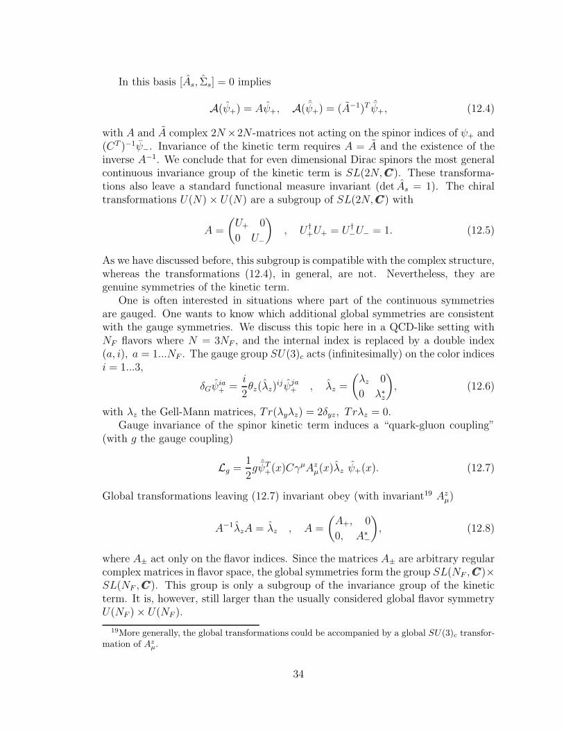
In this basis [As, Σs] = 0 implies

A(ψ+) = Aψ+, A( ˆψ+) = (A−1)T ˆψ+, (12.4)

with A and A complex 2N×2N -matrices not acting on the spinor indices of ψ+ and(CT )−1ψ−. Invariance of the kinetic term requires A = A and the existence of theinverse A−1. We conclude that for even dimensional Dirac spinors the most generalcontinuous invariance group of the kinetic term is SL(2N,CC). These transforma-tions also leave a standard functional measure invariant (det As = 1). The chiraltransformations U(N)× U(N) are a subgroup of SL(2N,CC) with

A =

(U+ 0

0 U−

), U †

+U+ = U †−U− = 1. (12.5)

As we have discussed before, this subgroup is compatible with the complex structure,whereas the transformations (12.4), in general, are not. Nevertheless, they aregenuine symmetries of the kinetic term.

One is often interested in situations where part of the continuous symmetriesare gauged. One wants to know which additional global symmetries are consistentwith the gauge symmetries. We discuss this topic here in a QCD-like setting withNF flavors where N = 3NF , and the internal index is replaced by a double index(a, i), a = 1...NF . The gauge group SU(3)c acts (infinitesimally) on the color indicesi = 1...3,

δGψia+ =

i

2θz(λz)

ijψja+ , λz =

(λz 0

0 λ∗z

), (12.6)

with λz the Gell-Mann matrices, Tr(λyλz) = 2δyz, T rλz = 0.Gauge invariance of the spinor kinetic term induces a “quark-gluon coupling”

(with g the gauge coupling)

Lg =1

2g ˆψT+(x)Cγ

µAzµ(x)λz ψ+(x). (12.7)

Global transformations leaving (12.7) invariant obey (with invariant19 Azµ)

A−1λzA = λz , A =

(A+, 0

0, A∗−

), (12.8)

where A± act only on the flavor indices. Since the matrices A± are arbitrary regularcomplex matrices in flavor space, the global symmetries form the group SL(NF , CC)×SL(NF , CC). This group is only a subgroup of the invariance group of the kineticterm. It is, however, still larger than the usually considered global flavor symmetryU(NF )× U(NF ).

19More generally, the global transformations could be accompanied by a global SU(3)c transfor-mation of Az

µ.

34

It is instructive to investigate the action of (12.8) on the Lorentz scalars,

Ls = ψ−Gw+λwψ+ + ψ+G

w−λwψ−, (12.9)

where w runs from 0 to 9 with λ0 =√

2/3 and Gw± arbitrary flavor matrices.

This follows from the transformation ψ+ → A+ψ+, ψ− → (A†−)

−1ψ−, ψ+ →(AT+)

−1ψ+, ψ− → A∗−ψ−. One finds

Gw+ → A†

−Gw+A+, G

w− → A−1

+ Gw−(A

†−)

−1. (12.10)

A flavor-singlet mass term is invariant for A†−A+ = 1. For unitary A± = U± this

reduces the symmetry to the vector-like flavor group U(NF ) with U+ = U−. For ourmore general transformation, a singlet mass term reduces SL(NF , CC)× SL(NF , CC)to the “diagonal” subgroup SL(NF , CC) with A

†− = A−1

+ .The fact that SL(NF , CC)×SL(NF , CC) transformations leave the covariant kinetic

term and therefore the classical QCD-action invariant does not yet guarantee thatthey are symmetries of the full quantum theory. For this property one also has torequire invariance of the functional measure. For a local gauge theory this is nottrivial. The measure has to be consistent with gauge symmetry which is not thecase for the “naive” SL(NF , CC)×SL(NF , CC) invariant measure. In fact, there is anincompatibility between part of the SL(NF , CC) × SL(NF , CC) transformations andgauge transformations, leading to an anomaly similar to the usual axial anomaly.(The axial U(1) transformations are actually part of SL(NF , CC) × SL(NF , CC).)This anomaly can be most easily seen by an investigation of the anomalous ’t Hooftmulti-fermion interaction [9]. The bilinear ϕ

(1)ab = ψ+bψ−a transforms as ϕ(1) →

(A†−)

−1ϕ(1)A−1+ and det ϕ(1) is invariant only for detA+(detA−)

∗ = 1. From ϕ(2)ab =

−ψ−bψ+a, ϕ(2) → A+ϕ

(2)A†− one sees that this is also the condition for the invariance

of det ϕ(2). It is straightforward to verify that the ’t Hooft interaction is invariantprecisely under the transformations obeying detA+(detA−)

∗ = 1.Consider QCD with two massless quarks, d = 4, NF = 2. The SL(2,C)-

transformations leaving the kinetic term and a singlet chiral condensate ψγψ in-variant read

ψ′L = AψL , ψ

′L = ψLA

−1,

ψ′R = AψR , ψ′

R = ψRA−1. (12.11)

The compact subgroup consists of the unitary transformations SU(2) × U(1). Atypical transformation that is not contained in the unitary transformations is thescaling by a real factor λ

ψ′ = λψ , ψ′ = λ−1ψ. (12.12)

It is allowed since ψu and ψv are independent Grassmann variables. The functionalmeasure is clearly invariant under this transformation. On the other hand, the scal-ing (12.12) is not compatible with the complex structure. A priori the compatibility

35

with the complex structure is not a restriction that has to be imposed. Symmetriesnot compatible with a complex structure are well known from other examples, as fora scalar field theory for a complex doublet which has the symmetry SO(4) and notonly SU(2)× U(1) - only the latter being compatible with the complex structure.

The question arises what happens if the extended symmetries are spontaneouslybroken. The QCD-action for our case is invariant under

ψ′L = AψL , ψ

′L = ψLA

−1,

ψ′R = BψR , ψ′

R = ψRB−1, (12.13)

while the regular complex matrices A,B obeying the constraint

det(AB∗) = 1 (12.14)

also leave the t’Hooft interaction invariant (A = A+, B = A−). The matrix A canbe represented as

A = exp(iαwτw) , αw ∈ C, (12.15)

with w = 0, 1, 2, 3, τ0 = 1, τk the Pauli matrices, and a similar representationB = exp(iβwτw). The difference to the unitary transformations arises from thecomplex parameters αw, βw instead of real ones. For infinitesimal transformationsthe condition (12.14) reads

α0 = β∗0 . (12.16)

The real part of α0 corresponds to the U(1) transformations representing fermionnumber conservation, while Im(α0) describes the scaling

ψ′L = λψL , ψ

′L = λ−1ψL,

ψ′R = λ−1ψR , ψ′

R = λψR. (12.17)

The scaling (12.12) is anomalous.We may try to represent the color singlet fermion bilinears with fermion number

zero by complex scalar fields

ϕab = ψa,iR ψb,iL , ϕab = −ψa,iL ψ

b,iR . (12.18)

If we want to guarantee that the real part of ϕ has a real expectation value, and thesame for iImϕ, consistency requires the identification ϕ = ϕ† (cf. sect. 7). On thelevel of bosonic fields only those transformations that are consistent with ϕ = ϕ†

can be consistently realized. From eq. (12.13) one infers

ϕ′ = (BT )−1ϕAT , ϕ′ = (AT )−1ϕBT ,

(ϕ†)′ = A∗ϕ†(B∗)−1. (12.19)

Consistency of ϕ = ϕ† requires A† = A−1, B† = B−1. Only this subgroup of unitarytransformations is relevant for the discussion of Goldstone bosons and we remainwith the usual scenario.

36

13 Conclusions

We have discussed a consistent mapping between Minkowski signature and euclideansignature for all types of spinors, in particular Majorana spinors and Majorana-Weyl spinors. This holds for arbitrary dimension d. In particular, no discontinuous“doubling of degrees of freedom” is needed when implementing the four-dimensionalMajorana spinors for Minkowski signature in the corresponding euclidean quantumfield theory. Analytic continuation is always possible.

Care has to be taken, however, for the proper choice of the complex structure.The hermitean conjugation for Minkowski signature has to be replaced by an in-volution θ for euclidean signature, which also involves the reflection of the timecoordinate. We find a modulo two periodicity in signature for the choice of thecomplex structure.

We define generalized Majorana spinors based on on a general mapping be-tween the independent Grassmann variables ψ and ψ. For Minkowski signaturethey coincide with the usual Majorana spinors. For euclidean signature, however,the generalized Majorana spinors differ from the real spinor representation of therotation group. The physical euclidean Majorana spinors are based on the notionof generalized Majorana spinors. They exist in precisely the same dimensions as forMinkowski signature. We also use this setting for a consistent implementation ofthe discrete symmetries parity, time reversal and charge conjugation for euclideanspinors and we discuss the issue of a “real action” and real expectation values.

Appendix A: Conventions for four dimensions

We collect here the most important relations for a particular representation of theClifford algebra in four dimensions. For euclidean signature (s = 0) the hermiteanmatrices γm are

γ0 =

(0 1

1 0

), γi =

(0 − iτiiτi 0

), γ = −γ0γ1γ2γ3 =

(1 0

0 − 1

). (A.1)

Here i = 1, 2, 3 and τi are the Pauli matrices. The hermitean generators of theeuclidean Lorentz (SO(4)-rotation) group read

σmn =i

2[γm, γn] = −2iΣmn =

(σmn+ 0

0 σmn−

), (A.2)

where

σij+ = σij− = −ǫijkτk,

σ0k+ = −τk , σ0k

− = τk. (A.3)

Corresponding representations for a Minkowski signature are easily obtainedfrom (A.1) by appropriate multiplications with a factor (−i). For s = 1 one mul-tiplies γ0 by a factor −i whereas for s = d − 1 the matrices γi are multiplied by

37

−i. The matrix γ = diag(1, 1,−1,−1) is the same for all signatures s. The phasefactor in eq. (2.11) is η = −1 for s = 0 and η = −i for s = 1. In particular, for aMinkowski signature s = 1 one has

γ0 =

(0 − i

−i 0

), σ0k

+ = iτk , σ0k− = −iτk , γ = −iγ0γ1γ2γ3. (A.4)

The matrix γ is usually called γ5 and the Weyl spinors are associated to lefthanded and right handed fermions

ψL = ψ+ =1 + γ

2ψ , ψR = ψ− =

1− γ

2ψ,

ψL = ψ+ =1− γ

2ψ , ψR = ψ− =

1 + γ

2ψ. (A.5)

We use the same kinetic term

Lkin = iψγµ∂µψ (A.6)

for all signatures s. Defining SE =∫d4xLkin and SM = −

∫d4xLkin the analytic

continuation discussed in sect. 3 implies e−SE = eiSM . For a Minkowski signatures = 1 we use the complex structure

ψ = ψ†γ0. (A.7)

By virtue of the relation 㵆γ0† = γ0γµ we observe that Lkin is hermitean, L†kin =

Lkin. In the notation of sect. 4 one has ǫ = 1 , D = D2 = γ0. For euclideansignature s = 0 and the choice H = H2 = −iγ0 the kinetic term is invariant underthe θ-reflection. In our conventions the discrete transformations therefore read

s = 0 : θψ(q) = Rψ(q) , θψ(q) = Rψ(q),

s = 1 : θMψ(q) = Rψ(q) , θM ψ(q) = Rψ(q), (A.8)

with

R = H∗(s=0) = H−1(s=0) = D∗(s=1) = D−1(s=1) =

(0 i

i 0

), (A.9)

or, for s = 1,

ψ∗(x) =

(0 i

i 0

)ψ(x). (A.10)

For our convention D = D2 for s = 1 the list of hermitean bilinears ψOjψ reads

Oj = i , γ , γm , γmγ , iσmn , σmnγ. (A.11)

For s = 0 , H = H2, this list also corresponds to terms that are invariant under θif an even number of indices m equals zero. On the other hand, these bilinears are

38

odd under θ for an odd number of zero-indices. In particular, a mass term takes theperhaps somewhat unusual form

Lm = mψRψL −m∗ψLψR, (A.12)

such that for real m the Dirac operator becomes20

D = iγµ∂µ +mγ. (A.13)

This convention simplifies many computations since the squared Dirac operator inmomentum space takes the simple form

D2 = qµqµ +m2. (A.14)

Such a simple form may constitute an advantage for euclidean lattice gauge theory,since m2 constitutes a gap in the spectrum of D2 and therefore acts as an effectiveinfrared cutoff for the fermion fluctuations.

The convention with D = iγµ∂µ+m would be obtained if we use D1, H1 insteadof D2, H2 (for s = 1, 0), with ψ = ψ†γ0γ instead of eq. (A.7). For fixed ψ† the twoconventions would be related by a simple redefinition of ψ , ψ′ = ψγ. However, thepartition function is defined as a functional integral over ψ and ψ as independentvariables. The two different choices for D should be interpreted as different choicesof the complex structure. In consequence, they are related by a transformation thatis not compatible with a given complex structure.

We note that a chiral rotation,

ψ → eiαγψ , ψ → ψeiαγ , (A.15)

induces a phase change of m in either convention but does not switch from oneconvention to the other. We may use this chiral phase in order to bring the massterm mγ in eq. (A.13) into the perhaps somewhat more conventional form im. (Thelatter corresponds to purely imaginary m in eq. (A.12).)

The charge conjugate spinor is defined as

ψc(q) = Cψ(q), ψc(q) = −Cψ(q). (A.16)

It involves the charge conjugation matrix (C ≡ C1) which is given by

C =

(c 0

0 − c

), c = iτ2 =

(0 1

−1 0

), c2 = −1 , (A.17)

and obeys (δ = −1)

(γm)T = −CγmC−1 , (σmn)T = −CσmnC−1 , [C, γ] = 0 ,

C = C∗ = −CT = −C† = −C−1 ,

CCT = −C2 = −CC∗ = 1. (A.18)

20This form is familiar from dimensional reduction of higher dimensional theories [12].

39

It is independent of the signature s.In presence of internal symmetries the generalized charge conjugation CW may

also act on internal spinor indices by a matrix G

CW (ψ) = ψc = GCψ , CW (ψ) = ψc = −G∗Cψ

G†G = 1 , G∗G = ǫG , C2W = ǫG. (A.19)

With

G =

(g+ 0

0 g−

)(A.20)

and g± unit matrices in (two-component) spinor space, acting only on internal in-dices, one obtains

ψc+ = g+cψ− , ψc− = −g−cψ+

ψc+ = g∗−cψ− , ψc− = −g∗+cψ+. (A.21)

The charge conjugation

CW (ψ±) = ψc± =1± γ

2ψc (A.22)

does not change the Lorentz representation of the spinors, corresponding to map-pings ψ+ → ψ− etc. Expressed in terms of ψ and ψ it acts in spinor space withoutan additional complex conjugation of the coefficients of the Grassmann algebra (incontrast to θ, θ).

For g+ = g− the bilinears transform as

CW (ψa+ψb−) = ψb+ψ

a− , CW (ψa−ψ

b+) = ψb−ψ

a+,

CW (ψa+γµψb+) = −ψb−γ

µψa− , CW (ψa−γµψb−) = −ψb+γ

µψa+,

CW (ψa+σµνψb−) = −ψb+σ

µνψa− , CW (ψa−σµνψb+) = −ψb−σ

µνψa+. (A.23)

Here ψ+ψ− stands for ψT+ψ− and corresponds to a contraction over spinor indicesand internal indices on which G acts. The additional “flavor indices” a, b denotedifferent species of spinors. (The matrix G acts as a matrix in flavor space.) Inparticular, a gauge covariant kinetic term for a vectorlike gauge symmetry,

SE = i

∫d4xψ+γ

µ(∂µ − igAµ)ψ+ + ψ−γµ(∂µ − igAµ)ψ−, (A.24)

is invariant under CW if the gauge field has negative C-parity, CW(Aµ(x)

)= −Aµ(x).

On the other hand, a gauge field with purely axial coupling (∼ γµγ) has positive Cparity.

The parity transformation (P = P2)

P(ψ(x0, ~x)

)= Pψ(x0,−~x) , P

(ψ(x0, ~x)

)= −ψ(x0,−~x)P, (A.25)

40

is represented by the matrix

P = γ0M γ = −iγ0E γ =

(0 − i

−i 0

)(A.26)

both for euclidean (s = 0) and Minkowski (s = 1) signature. The fermion bilinearstransform as

P : ψ−ψ+ → −ψ+ψ− , ψ+ψ− → −ψ−ψ+ ,

ψ+γµψ+ → −ψ−γ

µψ− , ψ−γµψ− → −ψ+γ

µψ+,

ψ−σµνψ+ → −ψ+σ

µνψ− , ψ+σµνψ− → −ψ−σ

µνψ+,

(A.27)

with γ0 = −γ0 , γi = γi , σ0i = −σ0i , σij − σij . For the combined CP-transformation this implies

CWP : ψa−ψb+ → −ψb+ψ

a− , ψa+ψ

b− → −ψb−ψ

a+ ,

ψa+γµψb+ → ψb+γ

µψa+ , ψa−γµψb− → ψb−γ

µψa− ,

ψa−σµνψb+ → ψb+σ

µνψa− , ψa+σµνψb− → ψb−σ

µνψa+,

(A.28)

and we note (CWP)2ψ(x) = −ψ(x).In our conventions a general mass term consistent with hermiticity (s = 1) or

Osterwalder-Schrader positivity (s = 0) reads

Lm = ψaM(H)ab γψb + ψaM

(A)ab ψb (A.29)

with M (H) and M (A) the hermitean and antihermitean parts of an arbitrary massmatrix Mab = M

(H)ab +M

(A)ab , (M (H))† = M (H) , (M (A))† = −M (A). It is invariant

under the charge conjugation CW for M = MT . Invariance with respect to parityrequires a hermitean mass matrix M = M † whereas CP-invariance follows for areal M = M∗. It is sufficient that these properties hold for an appropriate basis inspinor-space which may be realized by chiral transformations. In particular, if Mcan be transformed to a real diagonal form the possible violations of C, P and CPoccur in other sectors of the theory and are not related to the fermion masses.

Appendix B: Complex structures for real and com-

plex Grassmann algebra

A complex structure can be introduced for a real Grassmann algebra (real coefficientsa in eq. (4.9) or similar expressions) in a rather standard way. Let ψ be an arbitrary

41

vector of a 2N -dimensional vector space such that α1ψ1 + α2ψ2 is defined with realcoefficients α1,2. For example, the components ψα may be independent Grassmannvariables or real numbers. A complex structure is defined by two real 2N × 2Nmatrices K, I obeying

K2 = 1, I2 = −1, K, I = 0. (B.1)

Then K plays the role of complex conjugation, ψ∗ = Kψ, and I stands for themultiplication with i. Combining the conditions (B.1) one infers

TrK = 0. (B.2)

A typical example is

K =

(1 00 −1

), I =

(0 −11 0

), (B.3)

with the representation

ψ =

(ψRψI

), ψ∗ = Kψ =

(ψR−ψI

), Iψ =

(−ψIψR

). (B.4)

More generally, we may define the projections

ψR =1 +K

2ψ , ψI =

1−K

2ψ. (B.5)

Since ψR and ψI obey constraints, i.e. (1 + K)ψR = 2ψR, they have only N in-dependent components each. By a suitable change of basis we can always choosethe representation (B.3) and use ψR,I according to (B.3) as the independent com-

ponents. An isomorphism maps the 2N -component vector ψ to an N -componentcomplex vector ϕ,

ϕ = ψR + iψI , Kψ = ϕ∗ , Iψ = iϕ. (B.6)

The anticommutation property K, I = 0 guarantees (iϕ)∗ = −iϕ∗ according toKIψ = −IKψ.

Consider next linear transformations, ψ → ψ′ = Aψ, represented by real 2N×2Nmatrices A. For regular A they form a group. Only a subgroup is compatible withthe complex structure, namely those obeying

[A, I] = 0. (B.7)

This condition guarantees that the multiplication with i is represented by the samematrix I for ψ′ and ψ and commutes with all compatible linear transformations.One infers that A can be represented as

A = AR + AII, (B.8)

42

with AR and AI real N×N matrices. Furthermore, we define the complex conjugatematrix A∗ as a real 2N × 2N matrix by

A∗ = KAK. (B.9)

For transformations which are compatible with the given complex structure one has

A∗ = AR −AII, (B.10)

and we see that the “imaginary part” AI is odd under complex conjugation. Forthe particular representation (B.3) one has

A =

(AR, −AIAI , AR

), A∗ =

(AR, AI

−AI , AR

). (B.11)

For matrices compatible with the complex structure the isomorphism (B.6) re-flects complex multiplication with a N ×N matrix A

A = AR + iAI , ϕ→ Aϕ. (B.12)

Here the definition of A∗ guarantees

(Aϕ)∗ = A∗ϕ∗ = KAψ = A∗Kψ (B.13)

and the compatibility requirement (B.7) ensures

iAϕ = Aiϕ = IAψ = AIψ. (B.14)

It also implies that the real part of A is even under complex conjugation whereasthe “imaginary part” is odd

AR =1

2(A+ A∗) , AI =

1

2(A− A∗) , A = AR + AI , [AR, K] = 0 , AI , K = 0.

(B.15)We note that transformations A not obeying the compatibility condition (B.7) re-main well defined - they simply cannot be represented by a complex matrix multi-plication (B.12).

Next we turn to the case of complex coefficients αj as appropriate for our discus-sion of spinors in a complex Grassmann algebra. As an example, the 2N componentvector ψ may be composed from the Grassmann variables ψ and ψ

ψ =

(ψ

ψ

). (B.16)

Since multiplication with complex numbers is already defined for ψ it will not berepresented by a matrix I in this case. General linear transformations are nowrepresented by complex 2N × 2N matrices A, ψ → Aψ. However, the possibility

43

of multiplication with complex matrices does not yet specify the meaning of thecomplex conjugate of ψ. Only the definition of an involution ψ → ψ∗ fully definesthe complex structure.

A general complex structure is defined by the choice of a matrix K

ψ∗ = Kψ. (B.17)

As usual, the notion of complex conjugation also involves the complex conjugationof the linear coefficients

(α1ψ1 + α2ψ2)∗ = α∗

1Kψ1 + α∗2Kψ2, (B.18)

in accordance with (α1ψ1 + α2ψ2)∗ = α∗

1ψ∗1 + α∗

2ψ∗2. We require the conditions

K∗K = 1 , K† = K , TrK = 0. (B.19)

Here the first condition is necessary for the involutive property, (ψ∗)∗ = ψ, whereasthe second and third ensures an equal number of eigenvalues +1 and −1 for K andmay be dropped in a more general treatment.

Among the linear transformations ψ → ψ′ = Aψ only a subclass is compatiblewith a given complex structure K. Compatibility requires that complex conjugationfor ψ′ is represented by the same matrix K as for ψ, i.e. ψ′∗ = Kψ′. This results inthe compatibility condition21

KA = A∗K (B.20)

which ensures ψ′∗ = A∗ψ∗. Obviously, the class of compatible transformationsdepends on the specific choice of a complex structure K. They form a subgroup ofthe group of regular linear transformations.

References

[1] C. Wetterich, Nucl. Phys. B211 (1983) 177

[2] K. Osterwalder, R. Schrader, Comm. Math. Phys. 31 (1973) 83

[3] C. Wetterich, Phys. Rev. D74 (2006) 095009; Int. J. Mod. Phys. A23 (2008)1545; Mod. Phys. Lett. A23 (2008) 677; J. M. Schwindt, C. Wetterich, arXiv:0712.3405

[4] A. Hebecker, C. Wetterich, Phys. Lett. B574 (2003) 269;C. Wetterich, Phys. Rev. D70 (2004) 105004;C. Wetterich, Phys. Rev. Lett. 94 (2005) 011602

[5] C. Wetterich, Z. Phys. C48 (1990) 693

21Note the difference to eq. (B.9) which is a definition of A∗.

44

[6] F. Gliozzi, J. Scherk, D. Olive, Nucl. Phys. B122 (1977) 253

[7] G. Chapline and R. Slansky, Nucl. Phys. B209 (1982) 461

[8] C. Wetterich, Nucl. Phys. B234 (1984) 413

[9] G. ’t Hooft, Phys. Rev. D14 (1976) 3432

[10] E. Cartan, Theory of Spinors (Dover, N.Y., 1981)

[11] L. Alvarez-Gaume, An introduction to anomalies, Erice School Math. Phys.1985: 0093

[12] C. Wetterich, Nucl. Phys. B222 (1983) 20

45