Squared Eigenfunction Symmetriesfor Soliton Equations: Part II.Walter OevelFB 17 { MathematikUniversit�at PaderbornD 33095 Paderborn, GermanySandra CarilloDipartimento di Metodi e Modelli Matematiciper le Scienze ApplicateUniversit�a \La Sapienza"I 00161 Roma, ItalyAbstractNonlinear integrable evolution equations in 1 + 1 dimensions arisefrom constraints of the 2 + 1 dimensional hierarchies associated withthe Kadomtsev-Petviashvili (KP) equation, the modi�ed KP equationand the Dym equation, respectively. Links of B�acklund type andof reciprocal type are known to exist between the 2+1 dimensionalsystems. The corresponding links between the constrained ows arediscussed in a general framework. In particular, squared eigenfunctionsymmetries generated by solutions of the associated linear scatteringproblems are considered. The links between the soliton hierarchies areextended to these symmetries.MCS numbers: 58G37, 58F07, 35Q20, 35Q53Keywords: integrable systems, squared eigenfunctions, constrained KPhierarchy, KdV hierarchy, modi�ed KdV hierarchy, Dym hi-erarchy 1

1 IntroductionThe present article is a sequel to Ref. [12] which will be referred to as \PartI" in the following. The notation and terminology of Part I is used.B�acklund and Reciprocal Transformations have been introduced in con-nection with boundary value problems, as well as initial value problems,arising in connection with models mainly in Gas Dynamics and Fluid Me-chanics [13, 14]. For integrable systems, represented by a set of linear scat-tering equations, such transformations arise naturally as transformations ofthe underlying scattering operators. In Part I the Miura link between theKP hierarchy and the modi�ed KP hierarchy as well as the reciprocal linkbetween the modi�ed KP hierarchy and the 2+1 dimensional Dym hierar-chy were reviewed. These links were extended to the \squared eigenfunctionsymmetries", which are generated by products of eigenfunctions and adjointeigenfunctions, i.e., solutions of the underlying linear scattering problems.Building upon these 2+1 dimensional results, we now consider reductionsto 1+1 dimensions. In recent years there has been considerable interest inconstraints of the KP hierarchy induced by squared eigenfunctions [4, 5, 8,9, 15, 16, 17]. We adopt the approach to these systems via Lax operators ofpseudo-di�erential type which is a most convenient tool in 2+1 dimensions,also allowing a simple algebraic description of the constraints yielding 1+1dimensional reductions. 2

In Section 2 the constraints of the three basic hierarchies (KP, modi�edKP and Dym) are formulated. The Miura links as well as the reciprocallinks between the constrained ows are established. In Section 3 squaredeigenfunction symmetries for the constrained ows are considered, the Miurarelations and reciprocal links are extended to these symmetries.The family of 1+1 dimensional soliton systems residing in the 2+1 hi-erarchies is large. The approach of this article provides a uni�ed pictureof the connections between equations in this family. This is demonstratedby various examples in which the general results are applied to speci�c Laxoperators which correspond to speci�c integrable hierarchies.The general results can be extended to even larger families of integrableequations, when multicomponent versions of the 2+1 hierarchies are used asa starting point. The restriction to scalar Lax operators in Parts I and II ismainly motivated by the existence of the interesting third class of equations(the Dym hierarchy) which is present only in the scalar case.Proofs of all lemmata and theorems are given in the appendix.2 Constrained hierarchies and their linksIn this section we review the algebraic construction of the constrained hi-erarchies arising from symmetry reductions of the 2+1 dimensional systemsde�ning the KP, the mKP and the Dym hierarchies.3

We recall from Part I that the corresponding pseudo-di�erential Lax op-erators in 2+1 dimensions arek = 0 : LKP = @x + u@�1x + u2 @�2x + u3 @�3x + � � � ;k = 1 : LmKP = @x + v + v1 @�1x + v2 @�2x + � � � ;k = 2 : LDym = w @x + w0 + w1 @�1x + w2 @�2x + � � � ; (2.1)where the leading �elds u, v and w satisfy the various ows associated withthe KP, the mKP and the Dym equations, respectively, when the Lax dy-namics Ltn = [(Ln)�k; L] ; k = 0; 1 or 2 ; n 2 N (2.2)is imposed. Eigenfunctions � and adjoint eigenfunctions are de�ned assolutions of the associated linear evolution equations�tn = [(Ln)�k�] ; tn = �[@�kx (Ln)��k@kx ] : (2.3)Here, following the notation of Part I, the square brackets [operator function]indicate the action of a di�erential operator on a function. Important quan-tities associated with (adjoint) eigenfunctions are the potentials and bde�ned by the compatible equations( (k); �)x = (k)� ; ( (k); �)tn = res(@�1x (k)(Ln)�k�@�1x ) (2.4)andb( ; �(k))x = �(k) ; b( ; �(k))tn = res(@�1x @kx(Ln)�k@�kx �(k) @�1x ) ; (2.5)4

respectively, where, in turn, (k) denotes ; x or xx for k = 0; 1 or 2(similarly for �(k)). They are related byb( ; �(k)) = 8><>: ( ; �) (k = 0) ;�( x; �) + � (k = 1) ;( xx; �)� x�+ �x (k = 2) :As proven in Part I (lemma 2.2 and lemma 4.3), the compatibility conditionsof these equations are the linear evolutions (2.3) of the (adjoint) eigenfunc-tions.Reductions of the KP hierarchy induced by squared eigenfunctions[4, 5, 8, 9, 15, 16, 17] have been studied extensively in the literature. Such1+1 dimensional systems arise by imposing a symmetry constraint involvingsolutions of the associated linear scattering problems (2.3). The correspond-ing Lax operators are obtained by restricting the pseudo-di�erential tail ofthe (in�nite) pseudo-di�erential operators to some submanifold of a speci�cform. We formulate the constraints for the three classes of integrable hierar-chies associated with the labels k = 0; 1 and 2, respectively:Lemma 2.1: Consider L given by (2.1), k = 0; 1 or 2. Assume(LN )<k = mXj=1 qj@�1x rj@kx (2.6)for some N 2 N and some functions q1; : : : ; qm, r1; : : : ; rm. Then the dy-namicsLtn = [(Ln)�k ; L] ; qjtn = [(Ln)�k qj] ; rjtn = �[@�kx (Ln)��k@kx rj] (2.7)5

leaves the constraint (2.6) invariant.The constrained dynamics is 1+1 dimensional, since (2.7) represents nonlin-ear evolution equations in the independent variables tn and x for the N � 1�elds parametrizing (LN )�k and the �elds q1; : : : ; qm, r1; : : : ; rm.Example 2.2: We compute the equations of the �rst non-trivial owsin the hierarchies, obtained from qt2 = [(L2)�k q], rt2 = �[@�kx (L2)��k@kx r];associated with the following Lax operators (N = 1). For later conveniencewe use tildes (bars) for objects associated with k = 1 (k = 2):k = 0 : L = @x + q@�1x r : � qr �t2= � qxx + 2q2r�rxx � 2qr2 � (2.8)k = 1 : ~L = @x + ~q@�1x ~r@x + � : � ~q~r �t2= � ~qxx + 2~q~r~qx + �~qx�~rxx � 2~q~r~rx + �~rx �(2.9)~L = @x + ~q + @�1x ~r@x : � ~q~r �t2= � ~qxx + 2(~q + ~r) ~qx�~rxx + 2(~q + ~r) ~rx �(2.10)k = 2 : �L = �q@�1�x �r@2�x + (~�� �) �x@�x + � :� �q�r ��t2= � (�q�r + (~�� �) �x )2 �q�x�x�(�q�r + (~�� �) �x )2 �r�x�x � (2.11)�L = (�q + �r � �x2) @�x + �x� �r�x + @�1�x �r�x�x :� �q�r ��t2= � (�q + �r � �x2)2 �q�x�x�(�q + �r � �x2)2 �r�x�x � : (2.12)The constant parameters �; ~� are arbitrary. They will turn up naturally asspectral parameters in the following, when links between these equations and6

their hierarchies are considered. We note that all operators are of the form(2.6): k = 1 : ~L = @x + ~q@�1x ~r@x + �@�1x 1 @x ;~L = @x + ~q@�1x 1 @x + 1 @�1x ~r@x ;k = 2 : �L = �q@�1�x �r@2�x � �@�1�x �x@2�x + (�+ ~�) @�1�x 1 @2�x ;�L = 1 @�1�x �r@2�x � �x@�1�x �x@2�x + �q@�1�x 1 @2�x ;where the constant functions 1, � and ~� are admissible (adjoint) eigenfunc-tions satisfying (2.3) for the cases k = 1; 2. For k = 2 also �x is a solutionof (2.3). One encounters the AKNS system (2.8) for k = 0. The cases k = 1lead to a derivative nonlinear Schroedinger system (2.9) [3] and the Kaup-Broer system (2.10) [10]. In example 2.7 we will derive links (2.8) ! (2.10)! (2.12) between these equations and their higher ows, in example 2.9 links(2.8) ! (2.9) ! (2.11) will be established.Remark 2.3: The dynamics (2.7) of the constrained Lax operator (2.6)represents the compatibility condition of the linear equations�tn = [(Ln)�k�] ; [(LN )�k�] +Pj qjb(rj; �(k)) = �� (2.13)and tn = �[@�kx (Ln)��k@kx ] ; [@�kx (LN )��k@kx ]� (�1)kPj ( (k); qj)rj = � ;respectively. Here �; � 2 C are arbitrary spectral parameters and ( : ; :),b( : ; :) are the potentials de�ned by (2.4) and (2.5), respectively. The integro-7

di�erential spectral problem in (2.13) may be reformulated as a matrix prob-lem, e.g., for the scattering equation associated with L = @x+ q @�1x r, k = 0:�x + q b(r; �) = 2��b(r; �)x = r� ) () � b� �x = � 0 r�q 2� �� b� �() � 1 2 �x = � � �qr �� �� 1 2 �with 1 = exp(��x)�, 2 = exp(��x)b. The latter is the standard scatter-ing problem used to solve the AKNS hierarchy via Inverse Scattering tech-niques [1].Remark 2.4: Considering the squared eigenfunction symmetry (see theo-rem 4.1 and lemma 4.3 in Part I)Lz = [M;L] ; M =Pj qj@�1x rj@kxand �z =Pj qjb(rj; �(k)) ; z = (�1)kPj ( (k); qj)rjthe constraint (2.6) can be regarded as a symmetry reduction @=@tN =�@=@z of the 2+1 dimensional hierarchies discussed in Part I:Lz + LtN = [M + (LN )�k; L] = [M � (LN )<k; L] = 0 ;�z + �tN = �� ; z + tN = �� :We now consider the links k = 0 ! k = 1 ! k = 2 of the threeintegrable soliton hierarchies as reviewed by theorem 3.2 in Part I (see also[7, 11]) together with the class of constraints (2.6):8

Theorem 2.5: Let b( : ; :) be the potential de�ned by (2.5).a) (constrained KP ! constrained mKP): Let L = LKP satisfy the con-straint (LN )<0 = mXj=1 qj@�1x rj. Then, for any function �, the transformedoperator ~L = ��1L� satis�es the constraint(~LN)<1 = m+1Xj=1 ~qj@�1x ~rj@xwith ~qj = ��1qj ; ~rj = �b(rj; �) ; j = 1; : : : ;mand ~qm+1 = ��1� [(LN)�0�] + mXj=1 qjb(rj; �)� ; ~rm+1 = 1 :If L, qj, rj satisfy the constrained KP dynamics (2.7,k = 0) and � is an eigen-function (i.e., �tn = [(Ln)�0�]), then, according to theorem 3.2.a) in Part I,the gauge transformed Lax operator ~L satis�es the modi�ed KP dynamics~Ltn = [(~Ln)�1; ~L]. Further, ~qj and ~rj are new (adjoint) eigenfunctions:~qjtn = [(~Ln)�1 ~qj] ; ~rjtn = [@�1x (~Ln)��1 @x ~rj] ; j = 1; : : : ;m+ 1 :b) (constrained mKP! constrained Dym): Let ~L = LmKP satisfy theconstraint (~LN )<1 = mXj=1 ~qj@�1x ~rj@x. Then, for any transformation x! �x =~�(x), the transformed operator �L = ~L satis�es the constraint(�LN )<2 = m+1Xj=1 �qj@�1�x �rj@2�x9

with �qj = ~qj ; �rj = �b(~rj; ~�x) ; j = 1; : : : ;mand �qm+1 = [(~LN )�1 ~�] + mXj=1 ~qjb(~rj; ~�x) ; �rm+1 = 1 :We note �rj�x = �~rj for j = 1; : : : ;m. If ~L, ~qj, ~rj satisfy the modi�edKP dynamics (2.7,k = 1) and ~� is an eigenfunction (i.e., ~�tn = [(~Ln)�1 ~�]),then, according to theorem 3.2.b) in Part I, the transformed Lax operator�L satis�es the Dym dynamics �L�tn = [(�Ln)�2 ; �L] with respect to the newindependent variables �x and �tn = tn. Further, �qj and �rj are new (adjoint)eigenfunctions:�qj�tn = [(�Ln)�2 �qj] ; �rj�tn = �[@�2�x (�Ln)��2 @2�x �rj] ; j = 1; : : : ;m+ 1 :Here the projection �2 and the transposition � are to be taken with respectto the transformed symbol @�x = (~�x)�1 @x.Remark 2.6: One may choose one of the eigenfunctions in the pseudo-di�erential part of LN to generate the transformation. E.g., with � = qm thetransformation of the constrained KP hierarchy leads to(LN )<0 = mXj=1 qj@�1x rj !(~LN )<1 = m�1Xj=1 ~qj@�1x ~rj@x + 1 @�1x ~rm@x + ~qm+1@�1x 1 @x :10

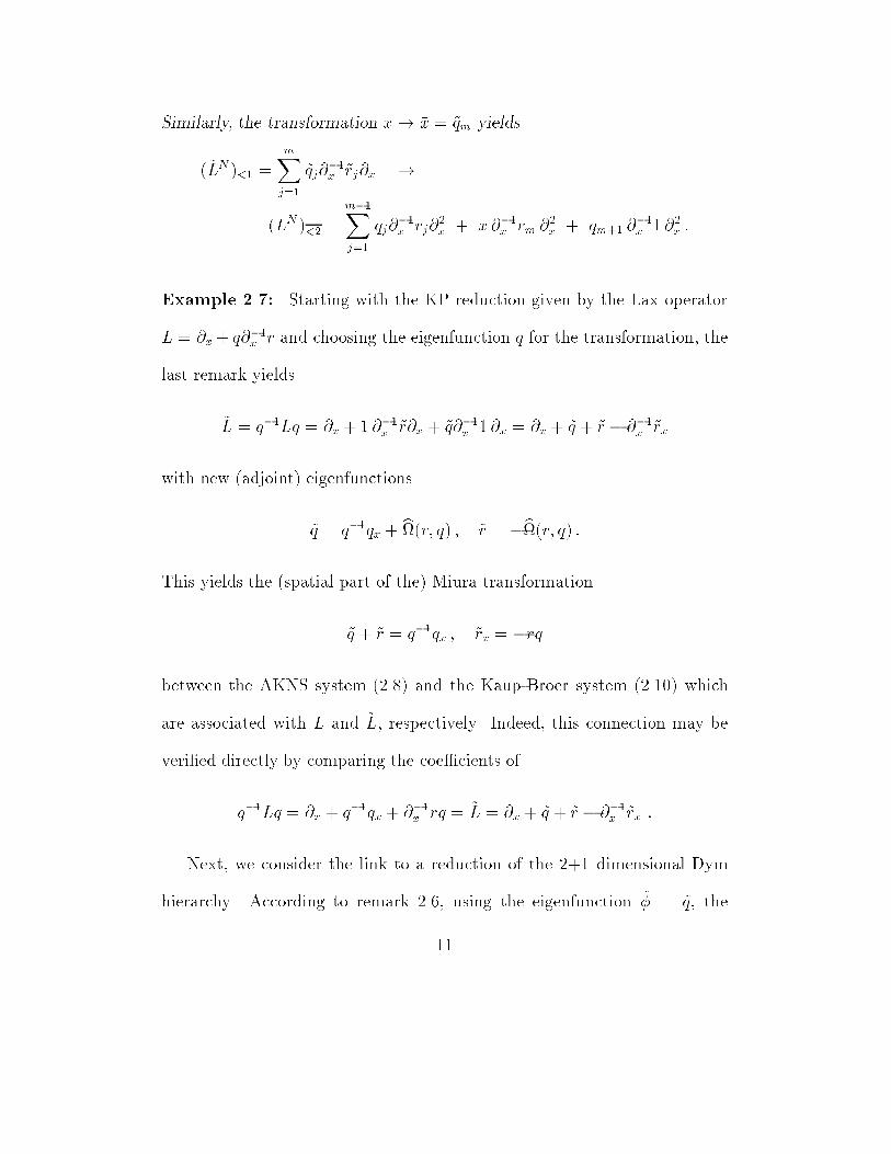
Similarly, the transformation x! �x = ~qm yields(~LN )<1 = mXj=1 ~qj@�1x ~rj@x !(�LN )<2 = m�1Xj=1 �qj@�1�x �rj@2�x + �x@�1�x �rm @2�x + �qm+1 @�1�x 1 @2�x :Example 2.7: Starting with the KP reduction given by the Lax operatorL = @x+ q@�1x r and choosing the eigenfunction q for the transformation, thelast remark yields~L = q�1Lq = @x + 1 @�1x ~r@x + ~q@�1x 1 @x = @x + ~q + ~r � @�1x ~rxwith new (adjoint) eigenfunctions~q = q�1qx + b(r; q) ; ~r = �b(r; q) :This yields the (spatial part of the) Miura transformation~q + ~r = q�1qx ; ~rx = �rqbetween the AKNS system (2.8) and the Kaup-Broer system (2.10) whichare associated with L and ~L, respectively. Indeed, this connection may beveri�ed directly by comparing the coe�cients ofq�1Lq = @x + q�1qx + @�1x rq = ~L = @x + ~q + ~r � @�1x ~rx :Next, we consider the link to a reduction of the 2+1 dimensional Dymhierarchy. According to remark 2.6, using the eigenfunction ~� = ~q, the11

transformation x! �x = ~q maps ~L to�L = 1 @�1�x �r@2�x � �x@�1�x b(1; ~qx)@2�x + �q@�1�x 1 @2�xwith�r = �b(~r; ~qx) ; �q = ~qx + ~q b(1; ~qx) + b(~r; ~qx) = ~qx + �x b(1; ~qx)� �r :We note b(1; ~qx)�x = 1, whence b(~r; ~qx) = �x+c with some arbitrary constantc. For c = 0 one �nds the Lax operator �L associated with (2.12), whence�r�x = ��r ; �q + �r � �x2 = ~qx = @�x@xyields a links between the Kaup-Broer system (2.10) and the system (2.12).This may be veri�ed directly by comparing the coe�cients of the Lax oper-ators~L = ~qx@�x + �x+ ~r � @�1�x ~r�x = �L = (�q + �r � �x2) @�x + �x� �r�x + @�1�x �r�x�x:Remark 2.8: Alternatively, one may apply theorem 2.5 with an eigenfunc-tion which satis�es a spectral equation (2.13). In this case the constraintsare transformed as follows:(LN )<0 = mXj=1 qj@�1x rj ! (~LN)<1 = mXj=1 ~qj@�1x ~rj@x + �and (~LN )<1 = mXj=1 ~qj@�1x ~rj@x ! (�LN )<2 = mXj=1 �qj@�1�x �rj@2�x + � �x @�x :12

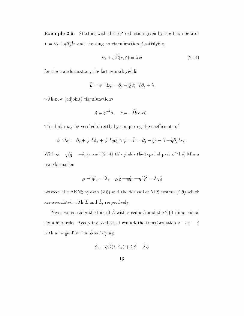
Example 2.9: Starting with the KP reduction given by the Lax operatorL = @x + q@�1x r and choosing an eigenfunction � satisfying�x + q b(r; �) = �� (2.14)for the transformation, the last remark yields~L = ��1L� = @x + ~q @�1x ~r@x + �with new (adjoint) eigenfunctions~q = ��1q ; ~r = �b(r; �) :This link may be veri�ed directly by comparing the coe�cients of��1L� = @x + ��1�x + ��1q@�1x r� = ~L = @x + ~q~r + �� ~q@�1x ~rx :With � = q=~q = �~rx=r and (2.14) this yields the (spatial part of the) Miuratransformation qr + ~q~rx = 0 ; qx~q � q~qx � q~r~q2 = � q~qbetween the AKNS system (2.8) and the derivative NLS system (2.9) whichare associated with L and ~L, respectively.Next, we consider the link of ~L with a reduction of the 2+1 dimensionalDym hierarchy. According to the last remark the transformation x! �x = ~�with an eigenfunction ~� satisfying~�x + ~q b(~r; ~�x) + � ~� = ~� ~�13

maps ~L = @x + ~q@�1x ~r@x + �@�1x 1 @x to�L = �q@�1�x �r@2�x � �@�1�x b(1; �x)@2�x + �� �x@�x = �q@�1�x �r@2�x + (~� � �) �x @�x + � ;where �q = ~q, �r = �b(~r; �x) and b(1; �x) = �x is chosen (note thatb(1; �x)�x = 1). One obtains the link�q = q ; �r�x = �~r ; @�x@x = �q�r + (~�� �) �xbetween the derivative NLS system (2.9) and the system (2.11). Indeed, thisis veri�ed directly by comparing the coe�cients of the Lax operators~L = ~�x@�x + ~q @�1�x ~r@�x + � = �L = (�q�r + (~� � �) �x) @�x � �q@�1�x �r�x@�x + � :Example 2.10: Links among well known 1 + 1 dimensional integrablehierarchies are retrieved easily from the general framework presented here.In particular, the B�acklund and reciprocal transformations relating the KdV,mKdV and Dym hierarchies [2, 6] follow naturally (see also [7]). Considerthe Lax operatorsL2 = @2x + 2u ; ~L2 = @2x + 2v@x ; �L2 = w2@2�x:With L = LKP, ~L = LmKP, �L = LDym they may be regarded as the pseudo-di�erential Lax operators (2.1), subject to the constraint (2.6) with N =2;m = 0. These operators generate the hierarchies of the KdV, the mKdV14

and the 1+1 dimensional Dym equation. In particular:(L2)t3 = [(L3)�0; L2] () 4ut3 = uxxx + 12uux (KdV);(~L2)t3 = [(~L3)�1; ~L2] () 4vt3 = vxxx � 6 v2vx (mKdV);(�L2)t3 = [(�L3)�2; �L2] () 4w�t3 = w3w�x�x�x (Dym):Invoking theorem 2.5.a) with an eigenfunction � satisfying the spectral equa-tion [L2�] = �xx + 2u� = 0 on computes ~L2 = ��1L2� = @2x + 2��1�x @x,i.e., v = ��1�x. Elimination of � by means of the spectral equation yieldsthe standard Miura link vx + v2 = �xx� = � 2ubetween the KdV solution u and the mKdV solution v. With an eigenfunction~� satisfying the spectral equation [~L2 ~�] = ~�xx + 2 v ~�x = 0 the reciprocaltransformation �x = ~� of theorem 2.5.b) yields �L2 = ~L2 = ~�2x@2�x, whencew = ~�x satis�es the Dym equation. Elimination of ~� by means of the spectralequation yields the reciprocal link between the mKdV solution v and the Dymsolution w characterized by@�x@x = ~�x = w ; w�x = wxw = �2 v ~�xw = � 2 v :3 Squared eigenfunction symmetries andtheir linksHere we consider the squared eigenfunction symmetries associated with theconstrained hierarchies of the previous section and discuss the additional15

conditions arising from the constraint (2.6).We assume that (adjoint) eigenfunctions �i, i, i = 1; : : : ;m1 satisfy-ing (2.3) are given. They generate the squared eigenfunction ow as de�nedin theorem 4.1 of Part I, which is compatible with the Lax dynamics (2.2).One has the following result concerning the invariance of the constraint (2.6):Theorem 3.1: The constraint (2.6) is invariant under the squared eigen-function ow Lz = h m1Xi=1 �i@�1x i@kx ; L i ;qjz = m1Xi=1 �ib( i; q(k)j ) ; rjz = (�1)k m1Xi=1 (r(k)j ; �i) i ;if �1; : : : ; �m1 and 1; : : : ; m1 satisfy[(LN )�k �i] + mXj=1 qjb(rj; �(k)i ) = �i�i ;[@�kx (LN)��k @kx i]� (�1)k mXj=1 ( (k)i ; qj)rj = �i iwith arbitrary spectral parameters �i 2 C .We �nally consider the standard constraints, where (LN )<k = 0, i.e., theLax operator LN is purely di�erential. According to theorem 3.2 of Part I onemay use an eigenfunction �, say, to trigger a transformation k = 0! k = 1or k = 1 ! k = 2 between the di�erent Lax hierarchies. According totheorem 4.6 in Part I the transformation is capable of linking the squaredeigenfunction symmetries, provided the triggering eigenfunction � satis�es16

a certain z-evolution. Speci�cally, for a squared eigenfunction symmetrygenerated by pairs of (adjoint) eigenfunctions �i and i, one has to imposethe ow �z =Pi �ib( i; �(k)) (3.15)on the triggering function. Following remark 2.8 it is natural to considersolutions of a spectral problem [LN�] = �� in order to avoid the appearanceof pseudo-di�erential terms introduced by the transformation triggered by�. One must guarantee that the ow (3.15) is consistent with the spectralcondition [LN�] = �� needed to preserve the di�erential character of theoperator. It turns out that this is granted via a particular choice of thearbitrary constant in the potentials b( i; �(k)). Indeed, due to the spectralequations the squared eigenfunction potentials can be represented in thefollowing way:Lemma 3.2: Let L satisfy the constraint (LN )<k = 0 for k = 0; 1 or2. Let L evolve according to (2.2), let �, be (adjoint) eigenfunctionssatisfying the dynamics (2.3) as well as the spectral equations 1 [LN�] = ��and [@�kx (LN )�@kx ] = � with spectral parameters �; � 2 C . Then, for� 6= �, the potentials de�ned by (2.4) and (2.5) may be chosen as( (k); �) = res(@�1x (k)LN�@�1x )� � �1No boundary conditions are assumed, i.e., � and need not be L2-functions.17

and b( ; �(k)) = res(@�1x @kxLN@�kx �(k) @�1x )� � �respectively.With these choices of the potentials one obtains:Theorem 3.3: Let L satisfy the constraint (LN )<k = 0 for k = 0; 1 or2. Let �1; : : : ; �m and 1; : : : ; m be (adjoint) eigenfunctions satisfying thespectral equations [LN�i] = �i�i and [@�kx (LN )�@kx i] = �i i, respectively.Consider the squared eigenfunction ow Lz = [Pi �i@�1x i@kx; L]. Then theequations [LN�] = �� and �z =Pi �ib( i; �(k))are compatible, provided that the potentials are chosen according to(� � �i) b( i; �(k)) = res(@�1x i@kxLN@�kx �(k)@�1x ) ; (3.16)or, equivalently, (�� �i)( (k)i ; �) = res(@�1x (k)i LN�@�1x ) :According to lemma 3.2 the requirement (3.16) is indeed consistent withthe de�ning equations (2.5) for � 6= �i.18

Example 3.4: Under the constraint (L2)<0 = 0 for L = LKP, i.e., L2 =@2x+2u, the KP hierarchy reduces to the KdV equation 4ut3 = uxxx+12uuxand its higher ows. Let �1; : : : ; �m and 1; : : : ; m solve[L2�i] = �ixx + 2u�i = �i�i ; [L2 i] = ixx + 2u i = �i i :They generate the squared eigenfunction ow (L2)z = [Pi �i@�1x i; L2] whichyields the systemuz = �Pi(�i i)x ; �ixx + u�i = �i�i ; ixx + u i = �i icharacterizing this symmetry of the KdV hierarchy2. We apply theorem4.6.a) of Part I with an eigenfunction � satisfying[L2�] = �xx + u� = �� ; �z =Xi �ib( i; �) ;where according to theorem 3.3 one has to chooseb( i; �) = res(@�1x iL2�@�1x )� � �i = i�x � ix�� � �i :for � 6= �i. If � = �i for some index i, then � = const i needs to be chosen3to grant the compatibility of the z- ow for � with [L2�] = ��. The map2The recursion operator R(u) : � ! �xx + 8u�+ 4ux Z x�1 � generates the hierarchy ofhigher KdV ows. We note R(u)uz = 4ux(P�i i)jx=�1 �4P�i�i i. For �i = 0 one hasR(u)uz = const ux, whence this special squared eigenfunction symmetry may be regardedas the �rst \negative ow" of the KdV hierarchy.3Note that eigenfunctions and adjoint eigenfunctions may be identi�ed, since L2 issymmetric. In this case the requirement (3.16) is satis�ed automatically (the residuevanishes due to the symmetry of L2), whence no condition on the arbitrary constant inb( i; �) arises. 19

L! ~L = ��1L� yields the reduction~L2 = @2x + 2��1�x@x + �of the modi�ed KP hierarchy, whence v = ��1�x satis�es the modi�ed KdVequation 4vt3 = vxxx � 6v2vx + 6�vx and its hierarchy. According to theo-rem 4.6.a) in Part I one obtains the modi�ed z- ow ~Lz = [Pj ~�i@�1x ~ i@x; ~L]with ~�i = ��1�i, ~ i = �b( i; �), which again satisfy the spectral equations[~L~�i] = �i ~�i and [@�1x (~L2)�@x ~ i] = �i ~ i. This Lax equation yields the systemvz = �Pi(~�i ~ i)x ; ~�ixx + 2v ~�ix = (�i � �)�i ; ~ ixx � 2v ~ ix = (�i � �) i ;representing the squared eigenfunction symmetry of the modi�ed KdV hi-erarchy4. For the special case given by only m = 2 pairs, where we choose~�1 = �1, ~ 2 = 1, �1 = �2 = �, one obtainsvz = ~ 1x � ~�2x ; ~ 1xx = 2v ~ 1x ; ~�2xx = �2v ~�2x ; (3.17)i.e., Vzx = a� b ; ax = 2Vxa ; bx = �2Vxb ;where V = ln(�) (i.e., v = Vx), a = ~ 1x and b = ~�2x. Integration yieldsa = f(z) exp(2V ), b = g(z) exp(�2V ) with arbitrary functions f(z) andg(z), i.e., Vzx = f(z) exp(2V )� g(z) exp(2V ) :4With v = ln(�)x the z-evolution is nothing but (��1(�z �P�ib( i; �)))x = 0.20

For f(z) = g(z) (characterized by ba = ~�2x ~ 1x = 1) one obtains the sinh-Gordon equation Vzx = sinh(2V ) after an appropriate rescaling of z, whichthus has been identi�ed as the special squared eigenfunction symmetry (3.17)of the modi�ed KdV hierarchy, which is subject to the constraint ~�2x ~ 1x = 1.For f(z) = 0 or g(z) = 0 one obtains the Liouville equations Vzx = exp(�2V ).A link to the squared eigenfunction symmetry of the constrained Dymhierarchy is obtained by theorem 4.6.b) in Part I. We choose an eigenfunction~� satisfying [~L2 ~�] = ~��, i.e.,~�xx + 2v ~�x = (~� � �) ~�and ~�z =Pi ~�ib( ~ i; ~�x) withb( ~ i; ~�x) = res(@�1x ~ i@x~L2@�1x ~�x@�1x )~� � �i = (~�� �) ~ i ~�� ~ ix ~�x~�� �i ;whence ~�z is compatible with [~L2 ~�] = ~�~� (theorem 3.3). The map ~L! �L =~L induced by �x = ~� yields the reduction�L2 = w2@2�x + (~�� �) �x @�x + � ; w = ~�xof the 2+1 dimensional Dym hierarchy, whence w satis�es the 1+1 dimen-sional Dym hierarchyw�t2 = (~���) (w��xw�x) ; 4w�t3 = w3w�x�x�x + 3 �x (~���)2 �1� �xw�xw � (3.18)and the corresponding higher isospectral ows. Applying theorem 4.6.b)of Part I the squared eigenfunction symmetry is obtained: �L�z =21

[Pi ��i@�1�x � i@2�x ; �L ] ; wherein �z = z, ��i = ~�i and� i = �b( ~ i; ~�x) = ~ ixw � (~�� �) �x ~ i~� � �i ; (3.19)which satisfy [�L2 ��i] = �i ��i and [@�2�x (�L2)��@2�x � i] = �i � i. This symmetry of(3.18) is characterized by the systemw�z =Pi ( ��i � iw�x � w(��i � i)�x ) ;w2 ��i�x�x + (~� � �)�x ��i�x = (�i � �) ��i ; w2 � i�x�x + (� � ~�)�x � i�x = (�i � ~�) � i :We �nally discuss the case arising from the sinh-Gordon equation, which isthe squared eigenfunction symmetryof the modi�ed KdV hierarchy generatedby two pairs (~�1; ~ 1) and (~�2; ~ 2) with ~�1 = �1, ~ 2 = 1, �1 = �2 = � and~�2x ~ 1x = 1. This leads to ��1 = �1 and � 2 = ��x from (3.19), whence thecorresponding equation compatible with the Dym hierarchy isw�z = w( � 1 + �x��2)�x � w�x( � 1 + �x��2) ;w2 ��2�x�x = (�� ~�) �x ��2�x ; w2 � 1�x�x = (~�� �) (�x � 1�x � � 1) ;constrained by �w2 ��2�x � 2�x�x = (� � ~�) ��2�x (�x � 1�x � � 1) = 1(note w ��2�x = ~�2x and w � 1�x�x = � ~ 1x). The transformation from (3.17) isgiven byw = @�x@x ; ��2 = ~�2 ; � 1 = ~ 1xw~�� � � �x ~ 1 ; w(w�x + 2v) = (~� � �) �x ;22

where the last equation is the spectral problem ~�xx + 2v ~�x = (~� � �)~� forw = ~�x.4 ConclusionsWe have studied the three families of 1+1 dimensional integrable solitonequations which arise as constrained ows of the KP hierarchy, the modi�edKP hierarchy and the Dym hierarchy, respectively. The Miura links betweenconstrained KP (k = 0) and constrained modi�ed KP (k = 1) equations aregiven by a simple gauge transformation of the associated Lax operators in-volving an eigenfunction. The reciprocal link between the systems of modi�edKP class (k = 1) and Dym class (k = 2) consists of a mere reparametrizationof the independent variable x by means of an eigenfunction. These resultsextend to the squared eigenfunction symmetries augmenting the soliton hi-erarchies. By specifying a Lax operator and applying the transformationsdescribed in the general theorems such links may be derived for large fami-lies of soliton hierarchies. Thus, the approach adopted here yields a uni�edpicture of transformations of constrained KP ows to related (modi�ed) in-tegrable systems. AcknowledgmentsThis work was partially supported by G.N.F.M. - C.N.R. and by the C.N.R.Contract n.95.01082.01. One of the authors (W.O.) wishes to acknowledge23

the DepartmentMetodi e Modelli Matematici per le Scienze Applicate, Uni-versity \La Sapienza", Rome, Italy, for their kind hospitality.References[1] M. J. Ablowitz and H. Segur: Solitons and the Inverse Scattering Trans-form, SIAM, Philadelphia, 1981.[2] S. Carillo and B. Fuchssteiner: Non commutative symmetries and newsolutions of the Harry Dym equation, in: Nonlinear Evolution Equa-tions: Integrability and Spectral Methods, A.Degasperis, A.P.Fordyand M.Lakhshmanan (eds.), p. 351-366, Manchester University Press,Manchester, 1990.[3] H.H. Chen, Y.C. Lee and C.S. Liu: Integrability of Nonlinear Hamil-tonian Systems by Inverse Scattering Method, Physica Scripta, 20, p.490{492, 1979.[4] Y. Cheng: Constraints of the KP hierarchy, J. Math. Phys., 33, p. 3774{3782, 1992.[5] Y. Cheng and Y. Li: The constraint of the KP equation and its specialsolutions, Phys. Lett. A, 157, p. 22{26, 1991.24

[6] B. Fuchssteiner and S. Carillo: Soliton structure versus singularity anal-ysis: third order completely integrable nonlinear equations in 1+1 dimen-sions, Physica A, 152, p. 467{510, 1989.[7] B.G. Konopelchenko and W. Oevel: An r-matrix Approach To Nonstan-dard Classes of Integrable Equations, Publ. RIMS, Kyoto Univ., 29, p.581{666, 1993.[8] B.G. Konopelchenko, J. Sidorenko and W. Strampp: (1+1)-dimensionalintegrable systems as symmetry constraint of (2+1)-dimensional sys-tems, Phys. Lett. A, 157, p. 17{21, 1991.[9] B.G. Konopelchenko and W. Strampp: The AKNS hierarchy as sym-metry constraint of the KP hierarchy, Inverse Problems, 7, p. L17{L24,1991.[10] B.A. Kupershmidt: Mathematics of dispersive water waves, Comm.Math. Phys., 99, p. 51{73, 1985.[11] W. Oevel and C. Rogers: Gauge Transformations and Reciprocal Linksin 2+1 Dimensions, Rev. Math. Phys., 5, p. 299{330, 1993.[12] W. Oevel and S. Carillo: Squared Eigenfunction Symmetries for SolitonEquations: Part I, preprint, 1997.25

[13] C. Rogers and W.F. Ames: Nonlinear Boundary Value Problems in Sci-ence and Engineering, Academic Press, Boston, 1989.[14] C. Rogers and W.F. Shadwick: B�acklund Transformations and their Ap-plications, Mathematics in Science and Engineering Vol. 161, AcademicPress, New York, 1982.[15] J. Sidorenko and W. Strampp: Symmetry constraints of the KP hierar-chy, Inverse Problems, 7, p. L37{L43, 1991.[16] J. Sidorenko and W. Strampp: Multicomponent integrable reductions inthe KP hierarchy, J. Math. Phys., 34, p. 1429{1446, 1993.[17] B. Xu: (1+1)-dimensional integrable Hamiltonian systems reduced fromsymmetry constraints of the KP hierarchy, Inverse Problems, 9, p. 355{363, 1993.AppendixIn the following computations we refer to the identities (A.1), : : : ,(A.9) asgiven in the appendix of Part I.26

Proof of lemma 2.1: With[ (Ln)�k; LN ]<k = [ (Ln)�k; (LN )<k]<k = [ (Ln)�k;Pj qj@�1x rj@kx]<k= Pj �(Ln)�kqj@�1x �<0rj@kx � Pj qj�@�1x rj@kx(Ln)�k�<k(A.8)= Pj [(Ln)�kqj] @�1x rj@kx � Pj qj�@�1x rj@kx(Ln)�k@�kx �<0 @kx(A.9)= Pj [(Ln)�kqj] @�1x rj@kx � Pj qj@�1x [@�kx (Ln)��k@kx rj] @kx= ddtnPj qj@�1x rj@kxone �ndsddtn �(LN )<k �Pj qj@�1x rj@kx� = [ (Ln)�k; LN ]<k � ddtnPj qj@�1x rj@kx = 0 ;whence the constraint (2.6) is invariant under the dynamics (2.7).Proof of theorem 2.5: a) One computes the new constraint(~LN )<1 = ��1(LN�)<1 = ��1(LN�)0 + ��1(LN )<0�= ��1[(LN)�0�] + ��1 mXj=1 qj@�1x rj�= ��1[(LN)�0�] + mXj=1 ��1qj ( b(rj; �)� @�1x b(rj; �)@x )= ��1 � [(LN )�0�] + mXj=1 qjb(rj; �)�+ mXj=1 ~qj@�1x ~rj@x :The dynamics of ~qj, ~rj with j = 1; : : : ;m is derived by a simple computation.The modi�ed KP dynamics of ~LN grants the eigenfunction dynamics for ~qm+1as well. 27

b) One computes the new constraint(�LN )<2 = (�LN)<1 + [(�LN)�1 �x] @�x = (�LN )<1 + [(~LN)�1 ~�] @�x= mXj=1 ~qj@�1x ~rj@x + [(~LN )�1 ~�] @�x= � mXj=1 �qj@�1�x �rj�x@�x + [(~LN )�1 ~�] @�x= � mXj=1 �qj�rj@�x + mXj=1 �qj@�1�x �rj@2�x + [(~LN)�1 ~�] @�x= � [(~LN)�1 ~�] + mXj=1 ~qjb(~rj; ~�x)�@�x + mXj=1 �qj@�1�x �rj@2�x :The dynamics of �qj, ~rj with j = 1; : : : ;m follows from a simple computation.The evolution equation for �qm+1 may then be derived from the Dym dynamicsof �L.Proof of theorem 3.1: The result is plausible, when the constraint isregarded as a symmetry reduction @tN + @z2 = 0, where @z2 represents thesquared eigenfunction symmetry generated by qj; rj. If a suitable z2- ow of�i; i is assumed, then, according to theorem 4.4 in Part I, z = z1, the ow@z commutes with @tN + @z2 , whence the constraint is invariant under @z.Indeed, an explicit computation yields:� (LN )<k �Pj qj@�1x rj@kx �z= Pi �i@�1x � [@�kx (LN )��k@kx i]� (�1)kPj ( (k)i ; qj)rj � @kx�Pi � [(LN )�k�i]�Pj qjb(rj; �(k)i )� @�1x i@kx = 0 :28

Proof of lemma 3.2: For R = res(@�1x (k)LN�@�1x ) one �ndsRx (A.1)= res( (k)LN�@�1x � @�1x (k)LN�)(A.3)= res( (k)LN�@�1x � �(LN)� (k) @�1x )(A.2)= (k)[LN�]� [(LN)� (k)]� = (� � �) (k)� :Further, with M = (Ln)�k:Rtn = res(@�1x (�[M� (k)]LN�+ (k)[M;LN ]�+ (k)LN [M�])@�1x )(A.3)= �res(@�1x �(LN)�(M� (k) � [M� (k)])@�1x )� res(@�1x (k)LN (M�� [M�])@�1x )= �res(@�1x �(LN)�(M� (k))�1@�1x )� res(@�1x (k)LN (M�)�1@�1x )(A.4)= �res(@�1x �(LN)�(M� (k) @�1x )�0)� res(@�1x (k)LN (M�@�1x )�0)(A.3,A.5)= res((@�1x (k)M)�0LN�@�1x ) + res((@�1x �M�)�0(LN )� (k) @�1x )(A.2)= ((@�1x (k)M)�0LN�)0 + ((@�1x �M�)�0(LN )� (k))0(A.6)= � [(@�1x (k)M)�0�] + � [(@�1x �M�)�0 (k)](A.7)= � (@�1x (k)M�)0 + � (@�1x �M� (k))0(A.2)= � res(@�1x (k)M�@�1x ) + � res(@�1x �M� (k) @�1x )(A.3)= (�� �) res(@�1x (k)M�@�1x ) :Consequently, one may choose the squared eigenfunction potential( (k); �) = R=(���). The results for b( ; �(k)) are veri�ed by an analogouscomputation. 29

Proof of theorem 3.3: Noting [LN�] = (LN�)0 we consider the spectralequation for � in the form � := res( (LN�� ��) @�1x ) = 0. One computes�z = Pi res��i@�1x i@kxLN�@�1x � LN�i@�1x i@kx�@�1x+ (LN � �)�ib( i; �(k)@�1x )� ;which, using equation (4.9) in Part I, yields�z =Pi �i nres(@�1x i@kxL�@�1x ) + (�1)k�i( (k)i ; �)� �b( i; �(k))o :It can be checked that the spectral equations for i and � lead tores(@�1x i@kxL�@�1x )� res(@�1x i@kxL@�kx �(k)@�1x )= 8<: 0 (k = 0)�i i� (k = 1)�i( i�x � ix�) (k = 2) 9=; = �i�b( i; �(k))� (�1)k( (k)i ; �)� ;and res(@�1x i@kxL�@�1x )� (�1)kres(@�1x (k)i L�@�1x )= 8<: 0 (k = 0)� i� (k = 1)�( i�x � ix�) (k = 2) 9=; = ��b( i; �(k))� (�1)k( (k)i ; �)� ;whence�z = Pi �i nres(@�1x i@kxLN@�kx �(k)@�1x )� (�� �i) b( i; �(k))o= (�1)k Pi �i n res(@�1x (k)i LN�@�1x )� (�� �i)( (k)i ; �)o = 0 :30