Quantum reference frame transformations as symmetries and ...

Quantum reference frame transformations as symmetriesand the paradox of the third particleMarius Krumm1,2, Philipp A. Hohn3,4, and Markus P. Muller1,2,5

1Institute for Quantum Optics and Quantum Information, Austrian Academy of Sciences, Boltzmanngasse 3, A-1090 Vienna,Austria

2Vienna Center for Quantum Science and Technology (VCQ), Faculty of Physics, University of Vienna, Vienna, Austria3Okinawa Institute of Science and Technology Graduate University, Onna, Okinawa 904 0495, Japan4Department of Physics and Astronomy, University College London, London, United Kingdom5Perimeter Institute for Theoretical Physics, 31 Caroline Street North, Waterloo ON N2L 2Y5, Canada

In a quantum world, reference frames are ulti-mately quantum systems too — but what does itmean to “jump into the perspective of a quantumparticle”? In this work, we show that quantumreference frame (QRF) transformations appearnaturally as symmetries of simple physical sys-tems. This allows us to rederive and generalizeknown QRF transformations within an alterna-tive, operationally transparent framework, andto shed new light on their structure and inter-pretation. We give an explicit description of theobservables that are measurable by agents con-strained by such quantum symmetries, and ap-ply our results to a puzzle known as the ‘para-

dox of the third particle’. We argue that it canbe reduced to the question of how to relation-ally embed fewer into more particles, and give athorough physical and algebraic analysis of thisquestion. This leads us to a generalization of thepartial trace (‘relational trace’) which arguablyresolves the paradox, and it uncovers importantstructures of constraint quantization within asimple quantum information setting, such as re-lational observables which are key in this reso-lution. While we restrict our attention to finiteAbelian groups for transparency and mathemat-ical rigor, the intuitive physical appeal of our re-sults makes us expect that they remain valid inmore general situations.

01

2

3

4

...

n-1

Cyclictranslations,

group Cn

12N=

3

<latexit sha1_base64="1uAEiDp0HbNGJ/CNa5TpdkIjuno=">AAAB9HicbVBNS8NAEJ3Ur1q/qh69BIvgqSRS0GPBiyepYG2hCWWznbRLN5tldyOU2L/hxYOCePXHePPfuG1z0NYHA4/3ZpiZF0nOtPG8b6e0tr6xuVXeruzs7u0fVA+PHnSaKYptmvJUdSOikTOBbcMMx65USJKIYycaX8/8ziMqzVJxbyYSw4QMBYsZJcZKwVMgNQsUEUOO/WrNq3tzuKvEL0gNCrT61a9gkNIsQWEoJ1r3fE+aMCfKMMpxWgkyjZLQMRliz1JBEtRhPr956p5ZZeDGqbIljDtXf0/kJNF6kkS2MyFmpJe9mfif18tMfBXmTMjMoKCLRXHGXZO6swDcAVNIDZ9YQqhi9laXjogi1NiYKjYEf/nlVdK5qPuNuu/fNWrN2yKPMpzAKZyDD5fQhBtoQRsoSHiGV3hzMufFeXc+Fq0lp5g5hj9wPn8ACoOSMA==</latexit>| i

<latexit sha1_base64="4PiHjr2w4kH2DzfJT0RJ/k24npg=">AAAB9HicbVBNS8NAFHypX7V+VT16WSyCp5JIQY9FLx4rWFtsQtlst+3SzSbsvggl9G948aAgXv0x3vw3btoctHVgYZh5jzc7YSKFQdf9dkpr6xubW+Xtys7u3v5B9fDowcSpZrzNYhnrbkgNl0LxNgqUvJtoTqNQ8k44ucn9zhPXRsTqHqcJDyI6UmIoGEUr+X5EcRyG2eOsr/rVmlt35yCrxCtIDQq0+tUvfxCzNOIKmaTG9Dw3wSCjGgWTfFbxU8MTyiZ0xHuWKhpxE2TzzDNyZpUBGcbaPoVkrv7eyGhkzDQK7WSe0Sx7ufif10txeBVkQiUpcsUWh4apJBiTvAAyEJozlFNLKNPCZiVsTDVlaGuq2BK85S+vks5F3WvUPe+uUWteF32U4QRO4Rw8uIQm3EIL2sAggWd4hTcndV6cd+djMVpyip1j+APn8wfta5IU</latexit>

Zn

Figure 1: The simplest example of this article’s setup: a discretization of wave functions in one spatial dimensionunder translation symmetry. The configuration space is the cyclic group Zn, and the one-particle Hilbert space isH = `2(Zn) ' Cn. We have N distinguishable particles in a joint quantum state |ψ〉 ∈ H⊗N , and we study QRFtransformations that switch between the “perspectives of the particles”.

Marius Krumm: [email protected] A. Hohn: [email protected] P. Muller: [email protected]

Accepted in Quantum 2021-06-18, click title to verify. Published under CC-BY 4.0. 1

arX

iv:2

011.

0195

1v2

[qu

ant-

ph]

21

Aug

202

1

https://quantum-journal.org/?s=Quantum%20reference%20frame%20transformations%20as%20symmetries%20and%20the%20paradox%20of%20the%20third%20particle&reason=title-click

https://quantum-journal.org/?s=Quantum%20reference%20frame%20transformations%20as%20symmetries%20and%20the%20paradox%20of%20the%20third%20particle&reason=title-click

mailto:[email protected]



Contents

1 Introduction 2

2 Quantum information vs. structural approach to reference frames 42.1 Describing physics with or without external relatum . . . . . . . . . . . . . . . . . . . . . . . . . 42.2 Communication scenarios illustrating the two approaches . . . . . . . . . . . . . . . . . . . . . 6

3 From symmetries to QRF transformations and invariant observables 93.1 G-systems and their symmetries . . . . . . . . . . . . . . . . . . . . . . . . . . . . . . . . . . . . . 103.2 Invariant observables and Hilbert space decomposition . . . . . . . . . . . . . . . . . . . . . . . 123.3 Group averaging states . . . . . . . . . . . . . . . . . . . . . . . . . . . . . . . . . . . . . . . . . . 143.4 Alignable states as states with a canonical representation . . . . . . . . . . . . . . . . . . . . . . 163.5 QRF transformations as symmetry group elements . . . . . . . . . . . . . . . . . . . . . . . . . . 163.6 Characterization of alignable states . . . . . . . . . . . . . . . . . . . . . . . . . . . . . . . . . . . 173.7 Alignable and relational observables . . . . . . . . . . . . . . . . . . . . . . . . . . . . . . . . . . 183.8 Communication scenario of the structural approach revisited . . . . . . . . . . . . . . . . . . . . 20

4 The paradox of the third particle and the relational trace 204.1 The non-uniqueness of invariant embeddings . . . . . . . . . . . . . . . . . . . . . . . . . . . . . 214.2 A class of invariant traces . . . . . . . . . . . . . . . . . . . . . . . . . . . . . . . . . . . . . . . . 244.3 Definition of the relational trace . . . . . . . . . . . . . . . . . . . . . . . . . . . . . . . . . . . . . 254.4 Relational resolution of the paradox . . . . . . . . . . . . . . . . . . . . . . . . . . . . . . . . . . 284.5 Comparison to the resolution by Angelo et al. . . . . . . . . . . . . . . . . . . . . . . . . . . . . . 28

5 Conclusions 29

Acknowledgments 32

References 32

1 Introduction

All physical quantities are described relative tosome frame of reference. But since all physical sys-tems are fundamentally quantum, reference framesmust ultimately be quantum systems, too. This sim-ple insight is of fundamental importance in a vari-ety of physical fields, including the foundations ofquantum physics [1–11], quantum information the-ory [12–19], quantum thermodynamics [20–28], andquantum gravity [29–37].

Recently, there has been a wave of interest ina specific approach to quantum reference frames(QRFs) that we can broadly classify as structural innature, including e.g. Refs. [38–49]. This approachextends the usual concept of reference frames by as-sociating them with quantum systems, and by de-scribing the physical situation of interest from the“internal perspective” of that quantum system. Forexample, if an interferometer has a particle travel-ling in a superposition of paths, how “does the par-

ticle see the interferometer” [50]?A central topic in this approach is the QRF de-

pendence of observable properties like superposi-tion, entanglement [38–40], classicality [39, 51, 52],or of quantum resources [53]. The correspondingQRF transformations admit an unambiguous defi-nition of spin in relativistic settings by transform-ing to a particle’s rest frame [46, 47], they describethe comparison of quantum clock readings [42, 45],and they yield an alternative approach to indefinitecausal structure [48,54]. Among other conceived ap-plications, they are furthermore conjectured to playa crucial rule in the implementation of a “quan-tum equivalence principle” [55] as well as in space-time singularity resolution [56] and the descriptionof early universe power spectra [57, 58] in quantumgravity and cosmology.

Despite the broad appeal, several fundamentaland conceptual questions remain open. For exam-ple, how should we make concrete sense of theidea of “jumping into the reference frame of a parti-


cle”? How are QRF transformations different fromany other unitary change of basis in Hilbert space?What kind of physical symmetry claim is associ-ated with the intuition that QRF changes “leavethe physics invariant”? Furthermore, there are re-ported difficulties to extend basic quantum infor-mation concepts into this context. For example,Ref. [50] describes a ‘paradox of the third particle’,an apparent inconsistency arising from determiningreduced quantum states in different QRFs.

In this article, we shed considerable light on allof these questions. We introduce a class of physi-cal systems subject to simple principles, and derivethe QRF transformations as the physical symmetriesof these systems. On the one hand, this gives usa transparent operational framework for QRFs thatmakes sense of the ‘jumping’ metaphor. On theother hand, it allows us to identify QRF transfor-mations as elements of a natural symmetry group,and to describe the structure of the observables thatare invariant under such transformations. This al-gebraic structure turns out to be key to elucidate theparadox of the third particle, which we do by intro-ducing a relational notion of the partial trace.

To keep the mathematical structures as trans-parent and accessible as possible, we restrict ourattention in this article to finite Abelian groups.But this already includes interesting physical set-tings like the discretization of translation-invariantquantum particles on the real line (see Figure 1),admitting the formulation of intriguing thoughtexperiments. Within this familiar quantum in-formation regime of finite-dimensional Hilbertspaces, we uncover a variety of structures that notonly shed light on the questions raised above, butthat also reflect important aspects of constraintquantization [59, 60], which for example underliescanonical approaches to quantum gravity andcosmology. This includes the notions of a “physicalHilbert space” encoding the relational states of thetheory [30, 61, 62], of relational and Dirac observ-ables [29–37, 42–45], and a simple demonstration ofhow constraints can in general arise from symme-tries. In particular, these notions will assume keyroles in our proposed resolution of the paradox ofthe third particle.

Overview and summary of results. Our article isorganized as follows. In Section 2, we begin with athorough operational comparison of this structuralapproach to QRFs with the more common quantuminformation approach. This sets the stage by em-bedding the notion of QRF transformations into a

broader conceptual framework.

<latexit sha1_base64="6S6WBk7iUa+MqlZtKhcadui8Yck=">AAACA3icbVBPS8MwHE3nvzn/VT2Jl+AQPI1WBnocevE4wbrBWkqapVtYkpYkFUYpXvwqXjwoiFe/hDe/jenWg24+CDze+/3I+70oZVRpx/m2aiura+sb9c3G1vbO7p69f3Cvkkxi4uGEJbIfIUUYFcTTVDPSTyVBPGKkF02uS7/3QKSiibjT05QEHI0EjSlG2kihfeT5VPgc6TFGLPeKMPclh2rKi9BuOi1nBrhM3Io0QYVuaH/5wwRnnAiNGVJq4DqpDnIkNcWMFA0/UyRFeIJGZGCoQJyoIJ+dUMBTowxhnEjzhIYz9fdGjrgyqSIzWYZVi14p/ucNMh1fBjkVaaaJwPOP4oxBncCyDzikkmDNpoYgLKnJCvEYSYS1aa1hSnAXT14mvfOW22657m272bmq+qiDY3ACzoALLkAH3IAu8AAGj+AZvII368l6sd6tj/lozap2DsEfWJ8/gmeX9A==</latexit>

U 2 Usym

symmetrygroup

Invariant states / observables

Alignable states

Relational states / observables

<latexit sha1_base64="iCyZNpvQiVNeICo4wqpJXUq2r5k=">AAAB/3icbVBNS8NAFHzxs9avqHjyslgETyWRgh6rXjxWsLbQhLDZbtulm03Y3RRKCPhXvHhQEK/+DW/+GzdtDto6sDDMvMebnTDhTGnH+bZWVtfWNzYrW9Xtnd29ffvg8FHFqSS0TWIey26IFeVM0LZmmtNuIimOQk474fi28DsTKhWLxYOeJtSP8FCwASNYGymwj70I6xHBPLvOg8yTEWJikgd2zak7M6Bl4pakBiVagf3l9WOSRlRowrFSPddJtJ9hqRnhNK96qaIJJmM8pD1DBY6o8rNZ/BydGaWPBrE0T2g0U39vZDhSahqFZrIIqxa9QvzP66V6cOVnTCSppoLMDw1SjnSMii5Qn0lKNJ8agolkJisiIywx0aaxqinBXfzyMulc1N1G3XXvG7XmTdlHBU7gFM7BhUtowh20oA0EMniGV3iznqwX6936mI+uWOXOEfyB9fkDReeWJA==</latexit>Ainv<latexit sha1_base64="FZMou7QX5vLeykUanzDJKI/oRgo=">AAACAHicbVBPS8MwHE39O+e/quDFS3AInkYrAz1OvXic4NxgLSXN0i0sSUuSCqX24Ffx4kFBvPoxvPltTLcedPNB4PHe78fv5YUJo0o7zre1tLyyurZe26hvbm3v7Np7+/cqTiUmXRyzWPZDpAijgnQ11Yz0E0kQDxnphZPr0u89EKloLO50lhCfo5GgEcVIGymwDz2O9Bgjll8WQe5JDpNxporAbjhNZwq4SNyKNECFTmB/ecMYp5wIjRlSauA6ifZzJDXFjBR1L1UkQXiCRmRgqECcKD+f5i/giVGGMIqleULDqfp7I0dcqYyHZrJMq+a9UvzPG6Q6uvBzKpJUE4Fnh6KUQR3Dsgw4pJJgzTJDEJbUZIV4jCTC2lRWNyW4819eJL2zpttquu5tq9G+qvqogSNwDE6BC85BG9yADugCDB7BM3gFb9aT9WK9Wx+z0SWr2jkAf2B9/gAoaZal</latexit>Aphys

<latexit sha1_base64="oNGgkMRW12WpYpkUDVUeT6b3kt8=">AAAB9XicdVBNS8NAEJ34WetX1aOXxSJ4CkkNrd4KXjxWsLbQhLLZbtqlm03c3RRK6O/w4kFBvPpfvPlv3LYRVPTBwOO9GWbmhSlnSjvOh7Wyura+sVnaKm/v7O7tVw4O71SSSULbJOGJ7IZYUc4EbWumOe2mkuI45LQTjq/mfmdCpWKJuNXTlAYxHgoWMYK1kQK/xfq5L2PExGTWr1Qd26vV6ucOWpLLRkGcOnJtZ4EqFGj1K+/+ICFZTIUmHCvVc51UBzmWmhFOZ2U/UzTFZIyHtGeowDFVQb44eoZOjTJAUSJNCY0W6veJHMdKTePQdMZYj9Rvby7+5fUyHV0EORNppqkgy0VRxpFO0DwBNGCSEs2nhmAimbkVkRGWmGiTU9mE8PUp+p90arbr2a5741WbXpFHCY7hBM7AhQY04Rpa0AYC9/AAT/BsTaxH68V6XbauWMXMEfyA9fYJs2uSfg==</latexit>

⇧inv<latexit sha1_base64="cFO3MjBWKSc70gnQMOo+VEYxG0c=">AAAB/HicbVBNS8NAEJ3Ur1q/Yj16WSyCp5JIQY8FLx4rWFtoQthsN+3S3STsbsQQ8le8eFAQr/4Qb/4bt20O2vpg4PHeDDPzwpQzpR3n26ptbG5t79R3G3v7B4dH9nHzQSWZJLRPEp7IYYgV5Symfc00p8NUUixCTgfh7GbuDx6pVCyJ73WeUl/gScwiRrA2UmA3vSnWXo8FhScFSqe5KgO75bSdBdA6cSvSggq9wP7yxgnJBI014Vipkeuk2i+w1IxwWja8TNEUkxme0JGhMRZU+cXi9hKdG2WMokSaijVaqL8nCiyUykVoOgXWU7XqzcX/vFGmo2u/YHGaaRqT5aIo40gnaB4EGjNJiea5IZhIZm5FZIolJtrE1TAhuKsvr5PBZdvttF33rtPqdqo86nAKZ3ABLlxBF26hB30g8ATP8ApvVmm9WO/Wx7K1ZlUzJ/AH1ucPw9yUrg==</latexit>

⇧phys

<latexit sha1_base64="H0yy4PbpcemljED48NSUWsWmf6Q=">AAACBHicbVBNS8NAEJ3Ur1q/ot70slgETyWRgr0IBS8eKxhbaELZbDft0s0m7G6EEgte/CtePCiIV3+EN/+N2zYHbX0w8Pa9GXbmhSlnSjvOt1VaWV1b3yhvVra2d3b37P2DO5VkklCPJDyRnRArypmgnmaa004qKY5DTtvh6Grqt++pVCwRt3qc0iDGA8EiRrA2Us8+8h78VDFfYjHg9PL3o2dXnZozA1ombkGqUKDVs7/8fkKymApNOFaq6zqpDnIsNSOcTip+pmiKyQgPaNdQgWOqgnx2wwSdGqWPokSaEhrN1N8TOY6VGseh6YyxHqpFbyr+53UzHTWCnIk001SQ+UdRxpFO0DQQ1GeSEs3HhmAimdkVkSGWmGgTW8WE4C6evEza5zW3XnPdm3q12SjyKMMxnMAZuHABTbiGFnhA4BGe4RXerCfrxXq3PuatJauYOYQ/sD5/AFflmGI=</latexit>

U | i = | i

<latexit sha1_base64="cFO3MjBWKSc70gnQMOo+VEYxG0c=">AAAB/HicbVBNS8NAEJ3Ur1q/Yj16WSyCp5JIQY8FLx4rWFtoQthsN+3S3STsbsQQ8le8eFAQr/4Qb/4bt20O2vpg4PHeDDPzwpQzpR3n26ptbG5t79R3G3v7B4dH9nHzQSWZJLRPEp7IYYgV5Symfc00p8NUUixCTgfh7GbuDx6pVCyJ73WeUl/gScwiRrA2UmA3vSnWXo8FhScFSqe5KgO75bSdBdA6cSvSggq9wP7yxgnJBI014Vipkeuk2i+w1IxwWja8TNEUkxme0JGhMRZU+cXi9hKdG2WMokSaijVaqL8nCiyUykVoOgXWU7XqzcX/vFGmo2u/YHGaaRqT5aIo40gnaB4EGjNJiea5IZhIZm5FZIolJtrE1TAhuKsvr5PBZdvttF33rtPqdqo86nAKZ3ABLlxBF26hB30g8ATP8ApvVmm9WO/Wx7K1ZlUzJ/AH1ucPw9yUrg==</latexit>

⇧phys

<latexit sha1_base64="oNGgkMRW12WpYpkUDVUeT6b3kt8=">AAAB9XicdVBNS8NAEJ34WetX1aOXxSJ4CkkNrd4KXjxWsLbQhLLZbtqlm03c3RRK6O/w4kFBvPpfvPlv3LYRVPTBwOO9GWbmhSlnSjvOh7Wyura+sVnaKm/v7O7tVw4O71SSSULbJOGJ7IZYUc4EbWumOe2mkuI45LQTjq/mfmdCpWKJuNXTlAYxHgoWMYK1kQK/xfq5L2PExGTWr1Qd26vV6ucOWpLLRkGcOnJtZ4EqFGj1K+/+ICFZTIUmHCvVc51UBzmWmhFOZ2U/UzTFZIyHtGeowDFVQb44eoZOjTJAUSJNCY0W6veJHMdKTePQdMZYj9Rvby7+5fUyHV0EORNppqkgy0VRxpFO0DwBNGCSEs2nhmAimbkVkRGWmGiTU9mE8PUp+p90arbr2a5741WbXpFHCY7hBM7AhQY04Rpa0AYC9/AAT/BsTaxH68V6XbauWMXMEfyA9fYJs2uSfg==</latexit>

⇧inv

<latexit sha1_base64="WIm3d6le63CjoMsGG83uqMoMEO8=">AAAB/nicbVDLSsNAFJ3UV62v+Ni5GSyCCymJFHQjFNy4rGBsoYllMpmkQyczYWYi1FD8FTcuFMSt3+HOv3HSdqGtBy6cOede5t4TZowq7TjfVmVpeWV1rbpe29jc2t6xd/fulMglJh4WTMhuiBRhlBNPU81IN5MEpSEjnXB4VfqdByIVFfxWjzISpCjhNKYYaSP17QPPlwMBvXs/QklC5GX57Nt1p+FMABeJOyN1MEO7b3/5kcB5SrjGDCnVc51MBwWSmmJGxjU/VyRDeIgS0jOUo5SooJhsP4bHRolgLKQpruFE/T1RoFSpURqazhTpgZr3SvE/r5fr+CIoKM9yTTiefhTnDGoByyhgRCXBmo0MQVhSsyvEAyQR1iawmgnBnT95kXTOGm6z4bo3zXrrdJZHFRyCI3ACXHAOWuAatIEHMHgEz+AVvFlP1ov1bn1MWyvWbGYf/IH1+QOQz5UL</latexit>

U⇢U † = ⇢

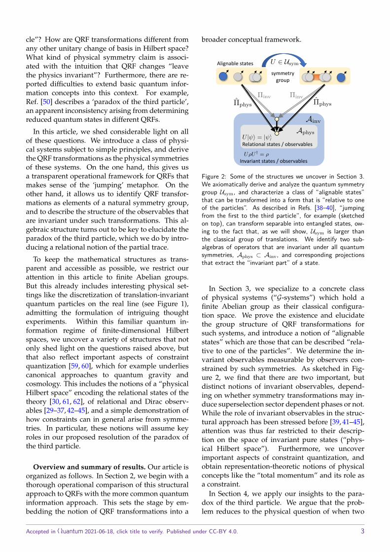
Figure 2: Some of the structures we uncover in Section 3.We axiomatically derive and analyze the quantum symmetrygroup Usym, and characterize a class of “alignable states”that can be transformed into a form that is “relative to oneof the particles”. As described in Refs. [38–40], “jumpingfrom the first to the third particle”, for example (sketchedon top), can transform separable into entangled states, ow-ing to the fact that, as we will show, Usym is larger thanthe classical group of translations. We identify two sub-algebras of operators that are invariant under all quantumsymmetries, Aphys ⊂ Ainv, and corresponding projectionsthat extract the “invariant part” of a state.

In Section 3, we specialize to a concrete classof physical systems (“G-systems”) which hold afinite Abelian group as their classical configura-tion space. We prove the existence and elucidatethe group structure of QRF transformations forsuch systems, and introduce a notion of “alignablestates” which are those that can be described “rela-tive to one of the particles”. We determine the in-variant observables measurable by observers con-strained by such symmetries. As sketched in Fig-ure 2, we find that there are two important, butdistinct notions of invariant observables, depend-ing on whether symmetry transformations may in-duce superselection sector dependent phases or not.While the role of invariant observables in the struc-tural approach has been stressed before [39, 41–45],attention was thus far restricted to their descrip-tion on the space of invariant pure states (“phys-ical Hilbert space”). Furthermore, we uncoverimportant aspects of constraint quantization, andobtain representation-theoretic notions of physicalconcepts like the “total momentum” and its role asa constraint.

In Section 4, we apply our insights to the para-dox of the third particle. We argue that the prob-lem reduces to the physical question of when two


groups of particles hold “the same relation” to eachother within two distinct configurations, such thatthe corresponding branches should interfere (seeFigure 6 on page 23). Mathematically, this corre-sponds to the question of how to embed the alge-bra of invariant N -particle observables into that ofN + M particles. We show that no unique answerto this question exists for the full set of invariant ob-servables in Ainv: the answer always depends onthe physical choice of how to determine the particlegroup interrelations operationally.

However, we show that a unique and natural em-bedding does exist for the subset of relational ob-servables in Aphys. The trick is to use a coherent su-perposition of all operationally conceivable particlegroup relations, and it turns out this constructionpreserves the algebraic structure of the N -particleobservables. We use this to define a relational no-tion of the partial trace which arguably resolves theparadox, and we compare this resolution to the oneproposed by Angelo et al. [50] before concluding inSection 5.

2 Quantum information vs. structuralapproach to reference frames

Let us begin with the main element that both thequantum information as well as the structural ap-proach to QRFs have arguably in common: a phys-ical system with a symmetry such that all observ-able quantities are invariant, or even fully relational.This is also the starting point of Refs. [7–10, 13, 19].

2.1 Describing physics with or without external re-latum

Consider a physical system S of interest. We as-sume that there is a set S of states in which thesystem S can be prepared. Furthermore, there is agroup of symmetry transformations Gsym that acts onS. Specifying S and Gsym amounts to making a spe-cific physical claim:

Assumption 1. If the system S is considered inisolation, then it is impossible to distinguish (evenprobabilistically) whether it has been prepared insome state ω or in another state G(ω). This is truefor all states ω ∈ S and all symmetry transforma-tions G ∈ Gsym.

’In isolation’ here means that any other physicalstructure to which S could be related is disregarded,

either because it does not exist in the first place, onedoes not have access to it, or it is deliberately ig-nored. This setting is schematically depicted in Fig-ure 3. Examples include:

(i) Minkowski spacetime of special relativity, withS the set of all possible states of matter (say,of classical point particles), and the Poincaregroup Gsym as the group of symmetry transfor-mations.

(ii) Electromagnetism in some bounded region ofspacetime. This is a gauge theory with Gsym thegroup of local U(1)-transformations as its sym-metry group.

(iii) A spin in quantum mechanics with Hilbertspace H and projective representation g 7→ Ugof the rotation group G = SO(3). Here, S is theset of density matrices ρ, and Gsym consists ofall maps of the form ρ 7→ UgρU

†g .

These three examples illustrate an important sub-tlety: to claim that ρ and Gρ are physically indistin-guishable, one needs to speak about ρ andGρ as dif-ferent objects in the first place. In other words, onehas to somehow define ρ and Gρ as distinct states.But in order to do so, one would need somethingexternal to the system S to refer to.

<latexit sha1_base64="aNGGLLuXvHYCYSkhPQLkWUQ8gVI=">AAAB6XicbVBNS8NAEJ3Ur1q/qh69LBbBU0mkoMeCF48ttrbQhrLZTtq1m03Y3Qgl9Bd48aAgXv1H3vw3btsctPXBwOO9GWbmBYng2rjut1PY2Nza3inulvb2Dw6PyscnDzpOFcM2i0WsugHVKLjEtuFGYDdRSKNAYCeY3M79zhMqzWPZMtME/YiOJA85o8ZKzftBueJW3QXIOvFyUoEcjUH5qz+MWRqhNExQrXuemxg/o8pwJnBW6qcaE8omdIQ9SyWNUPvZ4tAZubDKkISxsiUNWai/JzIaaT2NAtsZUTPWq95c/M/rpSa88TMuk9SgZMtFYSqIicn8azLkCpkRU0soU9zeStiYKsqMzaZkQ/BWX14nnauqV6t6XrNWqbfyPIpwBudwCR5cQx3uoAFtYIDwDK/w5jw6L86787FsLTj5zCn8gfP5A0mKjSI=</latexit>

S

external relatum

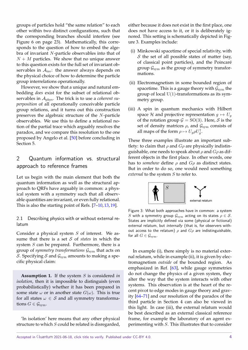
Figure 3: What both approaches have in common: a systemS with a symmetry group Gsym acting on its states ρ ∈ S.States are implicitly defined via some (physical or fictional)external relatum, but internally (that is, for observers with-out access to the relatum) ρ and Gρ are indistinguishable,for all G ∈ Gsym.

In example (i), there simply is no material exter-nal relatum, while in example (ii), it is given by elec-tromagnetism outside of the bounded region. Asemphasized in Ref. [63], while gauge symmetriesdo not change the physics of a given system, theyalter the way that the system interacts with othersystems. This observation is at the heart of the re-cent pivot to edge modes in gauge theory and grav-ity [64–71] and our resolution of the paradox of thethird particle in Section 4 can also be viewed inthis light. In case (iii), the external relatum wouldbe best described as an external classical referenceframe, for example the laboratory of an agent ex-perimenting with S. This illustrates that to consider


a system “in isolation” in the sense of Assumption 1does not imply that the system S is literally a physi-cally isolated system. It simply means that we havechosen to describe the system without the externalrelatum relative to which the action of the symme-try group is defined. Moreover, the setting does notimply that the agent who treats ρ and Gρ as indis-tinguishable is herself part of the system S, but onlythat the agent considers S without the external rela-tum.

Here we argue that the essential difference be-tween the two approaches to quantum referencesframes can succinctly be stated as follows:

The quantum information (QI) approach as ine.g. Refs. [12–17] emphasizes the fact that quantumstates are often only defined relative to an externalrelatum (as in Figure 3), and that this relatum mayultimately be a quantum system, too. This leadsto questions like: how can quantum information-theoretic protocols be performed in the absence ofa shared reference frame [12]? How well can quan-tum states stand in as resources of asymmetry ifthere is no shared frame [14, 15]? What are funda-mental quantum limits for communicating or align-ing reference frames [12]? Addressing questions asthese often involves encoding information in quan-tum states in an external relatum independent man-ner and, as such, requires external relatum indepen-dent descriptions of states.

The structural approach as in e.g. Refs. [38–40] isnot primarily concerned with operational protocols.While it shares the aim of external relatum indepen-dent descriptions of states with the QI approach, itgoes further: it disregards the external relatum al-together, and instead asks whether and how phys-ical subsystems of S can be promoted to an internalreference frame. This emphasizes the fact that thedistinction between quantum systems and their ref-erence frames is not fundamental, but merely con-ventional. It leads to questions like: what is thedescription of the quantum state relative to one ofits particles? Can we find a Hilbert space basis inwhich the description of the physics is simplified,e.g., in which superpositions of subsystems of in-terest may be removed? More generally, what arethe “QRF transformations” that relate the descrip-tions relative to different choices of internal refer-ence frame?

In the QI approach, it is usually not necessary totake the extra step to internal frame choices and toask how a system is described relative to one of its

subsystems, as we will explain shortly. It sufficesto focus on invariant properties of S which have ameaning relative to an arbitrary choice of externalframe in order to successfully carry out communi-cation tasks in the absence of a shared frame. Itis also worth emphasizing that there does not exista sharp distinction between the two approaches inthe body of literature on QRFs. Since the structuralapproach shares external relatum independent statedescriptions with the QI approach, there exist “hy-brid” works which arguably incorporate elementsfrom both. For example, Refs. [7–10,13,18,19,50] usestandard quantum information techniques to defineexternal relatum independent states, but also usethe latter to explore to some degree the question ofhow a quantum state is described relative to a sub-system. However, these works do not study the re-lations between the different such descriptions andthus, in particular, do not study the QRF transfor-mations.

The structural approach to QRFs is sometimes il-lustrated in ways that seem at first sight to be inconflict to the characterization above. For example,Figure 1 in Ref. [38] suggests to think of QRFs asphysically attached to an observer and its labora-tory (defined by its own quantum state), similarlyas reference frames in Special Relativity are oftenthought of as being attached to an observer (definedby its state of motion). QRF transformations wouldthen relate the descriptions of “quantum” observerswho are relative to each other in superposition in aWigner’s-friend-type fashion.

However, we will show below that the structuralframework of QRFs can be derived and analyzedexactly under an alternative and simpler interpre-tation. As we will elaborate and generalize below,choosing a QRF amounts to aligning one’s descrip-tion of the physics with respect to some choice of inter-nal quantum subsystem, such as the position of oneof the particles. Two different observers can choosetwo different subsystems (say, particles) that are rel-ative to each other in superposition, even if the ob-servers themselves are fully classical. Their descrip-tions will then be related by QRF transformations.The observer who assigns the quantum state maythus retain the status of a classical entity externalto the quantum system (at least in laboratory situa-tions), as illustrated in Figure 3. While more conser-vative, this new interpretation is operationally moreimmediate, and it is sufficient to reconstruct and ex-tend the full machinery of QRF transformations, aswe will see.

The characterization above is also in line withanother version of the structural approach: the


so-called perspective-neutral approach [39, 41–45]which, motivated by quantum gravity, is formu-lated in the language of constrained Hamiltoniansystems [59,60]. The starting point of this approachis a deep physical and operational motivation: takethe idea seriously that there are no reference frames, suchas rods or clocks, that are external to the universe. Toimplement this idea, one starts with a “kinematicalHilbert space” that defines all the involved quan-tum degrees of freedom and some gauge symmetry,but is interpreted as purely auxiliary. The absence ofexternal references is then implemented by restrict-ing to the gauge-invariant subset of states where thedescription becomes purely relational.

The actual mathematical machinery applied inthis approach still fits the description above: thekinematical Hilbert space can be viewed as beingdescribed relative to a fictional external relatum. Theinsight that there is nothing external to the uni-verse motivates to ask — purely formally at first —whether some of the internal degrees of freedom ofthe theory can be promoted to a frame of reference,such as a rod or clock. One may finally ask whetherobservers who are part of the theory may in facthave good operational access to that chosen frameof reference, but this is an additional (though impor-tant) question that we here regard as secondary.

2.2 Communication scenarios illustrating the twoapproaches

Before we turn to the structural approach in detail,and relate the verbal description above to the math-ematical formalization, let us elaborate on the dis-tinction by means of two communication scenarios.To do so, let us informally introduce some pieceof notation that we will later on define more for-mally. If ρ ∈ S is some state, denote by [ρ] the setof all states that are symmetrically equivalent to ρ,i.e. [ρ] := {Gρ | G ∈ Gsym}. The [ρ] can be viewedas equivalence classes of states, or as orbits of thesymmetry group.

Adapting the quantum information terminologyfrom Ref. [12], we refer to physical properties ofS that only depend on the equivalence class [ρ] asspeakable information. Being invariant under the ac-tion of Gsym and thus not requiring an external rela-tum in order to be defined, two agents can agree onthe description of these properties by classical com-munication even in the absence of a shared frame.By contrast, we refer to physical properties of S thatdepend on the concrete representative ρ from anequivalence class [ρ] of states as unspeakable informa-tion. These properties thus require the external rela-

tum to be meaningful and cannot be communicatedpurely classically between two agents who do notshare a frame.

2.2.1 The quantum information approach: communi-cating quantum systems

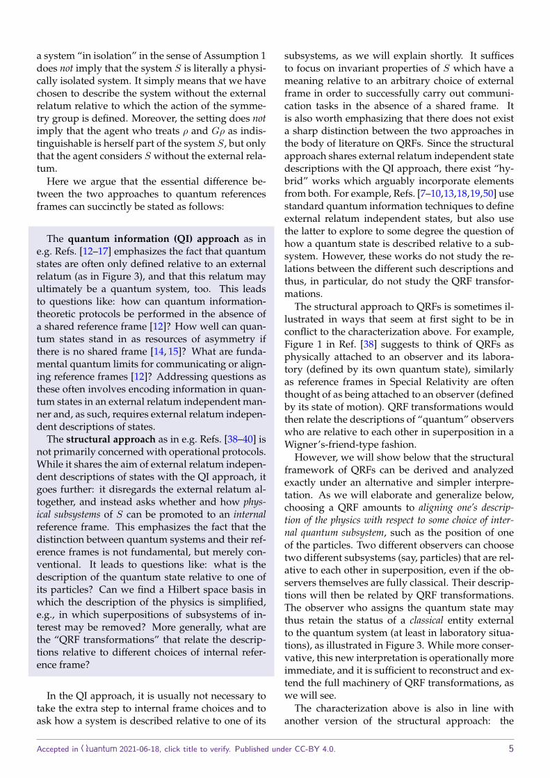
Consider the scenario in Figure 4. Alice holds aquantum system S that she has prepared in somestate ρ ∈ S(H), and S(H) denotes the density ma-trices on the corresponding Hilbert spaceH. We as-sume that there is a (for now, for simplicity) com-pact group G of symmetries and a projective rep-resentation G 3 g 7→ Ug such that G acts on S viaUg(ρ) = UgρU

†g . In this case, the symmetry group

is Gsym = {Ug | g ∈ G}. If we assume that Alice’squantum system S has the properties of Assump-tion 1, then the very definition of ρ is relative to herlocal frame of reference.

A B


S<latexit sha1_base64="vpH0EhT1tKcSDHKEIT/M9/r1fUc=">AAAB7HicbVBNS8NAEJ3Ur1q/qh69LBbBU0lE0GPBi8cKrS20oWy2m2bpfoTdjVBC/4IXDwri1R/kzX/jps1BWx8MPN6bYWZelHJmrO9/e5WNza3tnepubW//4PCofnzyaFSmCe0SxZXuR9hQziTtWmY57aeaYhFx2oumd4Xfe6LaMCU7dpbSUOCJZDEj2BbSUCdqVG/4TX8BtE6CkjSgRHtU/xqOFckElZZwbMwg8FMb5lhbRjid14aZoSkmUzyhA0clFtSE+eLWObpwyhjFSruSFi3U3xM5FsbMROQ6BbaJWfUK8T9vkNn4NsyZTDNLJVkuijOOrELF42jMNCWWzxzBRDN3KyIJ1phYF0/NhRCsvrxOelfN4LoZBA/XjVanzKMKZ3AOlxDADbTgHtrQBQIJPMMrvHnCe/HevY9la8UrZ07hD7zPH7xXjpI=</latexit>⇢

<latexit sha1_base64="onLwHmJUUnYaGFa+UJ6Qp4A/eVI=">AAAB+3icbVBNS8NAFHzxs9avVI9eFotQLyWRgh4LInis0NpCE8pmu2mXbjZhd6OU2J/ixYOCePWPePPfuGlz0NaBhWHmPd7sBAlnSjvOt7W2vrG5tV3aKe/u7R8c2pWjexWnktAOiXksewFWlDNBO5ppTnuJpDgKOO0Gk+vc7z5QqVgs2nqaUD/CI8FCRrA20sCueBHWY4J5djOreXIcnw/sqlN35kCrxC1IFQq0BvaXN4xJGlGhCcdK9V0n0X6GpWaE01nZSxVNMJngEe0bKnBElZ/No8/QmVGGKIyleUKjufp7I8ORUtMoMJN5ULXs5eJ/Xj/V4ZWfMZGkmgqyOBSmHOkY5T2gIZOUaD41BBPJTFZExlhiok1bZVOCu/zlVdK9qLuNuuveNarNdtFHCU7gFGrgwiU04RZa0AECj/AMr/BmPVkv1rv1sRhds4qdY/gD6/MHhoCUCQ==</latexit>E(⇢)

Figure 4: A communication scenario within the quantuminformation approach as in Ref. [12]. The focus is on send-ing and recovering actual physical (quantum) states that aredefined (as in Assumption 1) with respect to some exter-nal relatum, i.e. that may contain unspeakable information.This task becomes interesting if Alice’s and Bob’s referenceframes are initially unaligned.

Suppose that Alice sends the quantum systemphysically to Bob. Since Bob’s reference frame is notaligned with Alice’s, he will describe the situationas receiving a randomly sampled representative ofthe equivalence class [ρ]. Thus, he will assign thestate E(ρ) :=

∫G UgρU

†g dg to the incoming quantum

system.The QI approach is concerned with the possibility

to devise protocols that can be performed even inthe absence of a shared reference frame. For exam-ple, the task to send quantum information from Al-ice to Bob can be accomplished by encoding it into adecoherence-free subspace, i.e. a subsystem within theset of ρ ∈ S(H) for which E(ρ) = ρ (see e.g. Ref. [12,Sec. A.2] for a concrete example). Another possibil-ity to do so is by sending several quantum systems(e.g. spin-coherent states) that break the symmetry,and that allow Bob to partially correlate his refer-ence frame with Alice’s via suitable measurementson those states. The key to carrying out communica-tion protocols without a shared frame is thus to fo-


cus on invariant physical properties that are mean-ingful in any external laboratory frame. This doesnot require describing S relative to one of its sub-systems.

Nevertheless, in the QI approach, the quantumnature of reference frames is sometimes taken intoaccount, for example, by “quantizing” them to over-come superselection rules that arise in the absenceof a shared classical frame [12]. This “quantization”of a frame means adding a reference quantum sys-tem R to the system of interest S in order to definerelative quantities between R and S, such as rela-tive phases [12] or relative distances [13, 19], thatare invariant under Gsym and thereby meaningfulrelative to any external laboratory frame. In a com-munication scenario between two parties Alice andBob who do not share a classical frame, the refer-ence system R will typically be communicated to-gether with S. While this also constitutes an inter-nalization of a frame in the sense thats the referencesystem R is now a quantum system too, it is stillexternal to S. Furthermore, since the relative quan-tities between R and S are meaningful relative toany external laboratory frame with respect to whicha measurement will be carried out, it is not neces-sary to take an extra step and ask how S is described“from the perspective” of R in order for Alice andBob to succeed in their communication task.

In summary, in the QI approach, the quantumsystem S of interest (say, a set of spins) is treatedas a distinct entity from the reference frame (say, agyroscope). Thus, “QRF transformations” relatingdescriptions relative to different subsystems (whichmay be in relative superposition) are typically notstudied in this approach.1 The focus is on correlating(aligning) Alice’s and Bob’s frames, and it is the ab-sence of alignment that is modelled by the G-twirl,ρ 7→ E(ρ). The external relatum independent (or re-lational) state descriptions of the QI approach arethus the incoherently group-averaged states.

1This includes Ref. [18], where transformations between dif-ferent “quantized” reference systems R1 and R2 are studied.However, in the spirit of the QI approach, the derived trans-formations proceed between different invariant states (i.e. es-sentially G-twirls of ρS ⊗ ρRi , i = 1, 2) and are thus not trans-formations between descriptions of the quantum state of Srelative to different choices of subsystem, as we will see themlater. In particular, the descriptions of the quantum state ofS relative to different subsystems will be different descriptionsof one and the same invariant state.

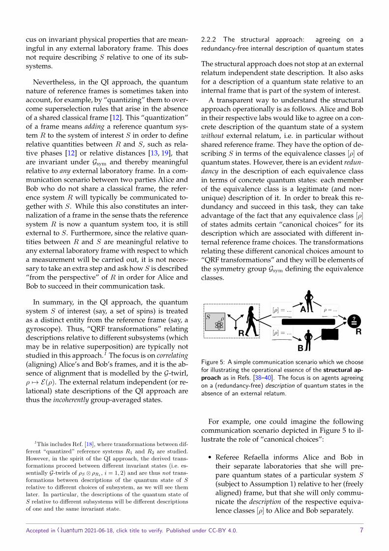
2.2.2 The structural approach: agreeing on aredundancy-free internal description of quantum states

The structural approach does not stop at an externalrelatum independent state description. It also asksfor a description of a quantum state relative to aninternal frame that is part of the system of interest.

A transparent way to understand the structuralapproach operationally is as follows. Alice and Bobin their respective labs would like to agree on a con-crete description of the quantum state of a systemwithout external relatum, i.e. in particular withoutshared reference frame. They have the option of de-scribing S in terms of the equivalence classes [ρ] ofquantum states. However, there is an evident redun-dancy in the description of each equivalence classin terms of concrete quantum states: each memberof the equivalence class is a legitimate (and non-unique) description of it. In order to break this re-dundancy and succeed in this task, they can takeadvantage of the fact that any equivalence class [ρ]of states admits certain “canonical choices” for itsdescription which are associated with different in-ternal reference frame choices. The transformationsrelating these different canonical choices amount to“QRF transformations” and they will be elements ofthe symmetry group Gsym defining the equivalenceclasses.


S <latexit sha1_base64="vpH0EhT1tKcSDHKEIT/M9/r1fUc=">AAAB7HicbVBNS8NAEJ3Ur1q/qh69LBbBU0lE0GPBi8cKrS20oWy2m2bpfoTdjVBC/4IXDwri1R/kzX/jps1BWx8MPN6bYWZelHJmrO9/e5WNza3tnepubW//4PCofnzyaFSmCe0SxZXuR9hQziTtWmY57aeaYhFx2oumd4Xfe6LaMCU7dpbSUOCJZDEj2BbSUCdqVG/4TX8BtE6CkjSgRHtU/xqOFckElZZwbMwg8FMb5lhbRjid14aZoSkmUzyhA0clFtSE+eLWObpwyhjFSruSFi3U3xM5FsbMROQ6BbaJWfUK8T9vkNn4NsyZTDNLJVkuijOOrELF42jMNCWWzxzBRDN3KyIJ1phYF0/NhRCsvrxOelfN4LoZBA/XjVanzKMKZ3AOlxDADbTgHtrQBQIJPMMrvHnCe/HevY9la8UrZ07hD7zPH7xXjpI=</latexit>⇢

<latexit sha1_base64="pCea5MGpdIWdI4n1SVVtoaLxEoI=">AAAB8nicbVBNS8NAEJ3Ur1q/qh69LBbBU0ikUC9CQQ8eK1hbTEPZbDft0s1u2N0IJfRfePGgIF79Nd78N27bHLT1wcDjvRlm5kUpZ9p43rdTWlvf2Nwqb1d2dvf2D6qHRw9aZorQNpFcqm6ENeVM0LZhhtNuqihOIk470fh65neeqNJMinszSWmY4KFgMSPYWOkx6KmRDK9c1+1Xa57rzYFWiV+QGhRo9atfvYEkWUKFIRxrHfheasIcK8MIp9NKL9M0xWSMhzSwVOCE6jCfXzxFZ1YZoFgqW8Kgufp7IseJ1pMksp0JNiO97M3E/7wgM/FlmDORZoYKslgUZxwZiWbvowFTlBg+sQQTxeytiIywwsTYkCo2BH/55VXSuXD9uuv7d/Va86bIowwncArn4EMDmnALLWgDAQHP8ApvjnZenHfnY9FacoqZY/gD5/MH6XCQPQ==</latexit>

[⇢] = ...

R

A

B

<latexit sha1_base64="pCea5MGpdIWdI4n1SVVtoaLxEoI=">AAAB8nicbVBNS8NAEJ3Ur1q/qh69LBbBU0ikUC9CQQ8eK1hbTEPZbDft0s1u2N0IJfRfePGgIF79Nd78N27bHLT1wcDjvRlm5kUpZ9p43rdTWlvf2Nwqb1d2dvf2D6qHRw9aZorQNpFcqm6ENeVM0LZhhtNuqihOIk470fh65neeqNJMinszSWmY4KFgMSPYWOkx6KmRDK9c1+1Xa57rzYFWiV+QGhRo9atfvYEkWUKFIRxrHfheasIcK8MIp9NKL9M0xWSMhzSwVOCE6jCfXzxFZ1YZoFgqW8Kgufp7IseJ1pMksp0JNiO97M3E/7wgM/FlmDORZoYKslgUZxwZiWbvowFTlBg+sQQTxeytiIywwsTYkCo2BH/55VXSuXD9uuv7d/Va86bIowwncArn4EMDmnALLWgDAQHP8ApvjnZenHfnY9FacoqZY/gD5/MH6XCQPQ==</latexit>

[⇢] = ...

<latexit sha1_base64="Wk+sdrAgN4fh2yccBzb5X+M/QOg=">AAAB8HicbVBNSwMxEJ2tX7V+VT16CRbB07IRQS9CwYsnqWBtoV1KNs22odlkTbJCWfonvHhQEK/+HG/+G9N2D9r6YODx3gwz86JUcGOD4NsrrayurW+UNytb2zu7e9X9gwejMk1ZkyqhdDsihgkuWdNyK1g71YwkkWCtaHQ99VtPTBuu5L0dpyxMyEDymFNindTu6qG68n2/V60FfjADWia4IDUo0OhVv7p9RbOESUsFMaaDg9SGOdGWU8EmlW5mWEroiAxYx1FJEmbCfHbvBJ04pY9ipV1Ji2bq74mcJMaMk8h1JsQOzaI3Ff/zOpmNL8OcyzSzTNL5ojgTyCo0fR71uWbUirEjhGrubkV0SDSh1kVUcSHgxZeXSevMx+c+xnfntfptkUcZjuAYTgHDBdThBhrQBAoCnuEV3rxH78V79z7mrSWvmDmEP/A+fwCEl497</latexit>⇢ = ...

<latexit sha1_base64="Wk+sdrAgN4fh2yccBzb5X+M/QOg=">AAAB8HicbVBNSwMxEJ2tX7V+VT16CRbB07IRQS9CwYsnqWBtoV1KNs22odlkTbJCWfonvHhQEK/+HG/+G9N2D9r6YODx3gwz86JUcGOD4NsrrayurW+UNytb2zu7e9X9gwejMk1ZkyqhdDsihgkuWdNyK1g71YwkkWCtaHQ99VtPTBuu5L0dpyxMyEDymFNindTu6qG68n2/V60FfjADWia4IDUo0OhVv7p9RbOESUsFMaaDg9SGOdGWU8EmlW5mWEroiAxYx1FJEmbCfHbvBJ04pY9ipV1Ji2bq74mcJMaMk8h1JsQOzaI3Ff/zOpmNL8OcyzSzTNL5ojgTyCo0fR71uWbUirEjhGrubkV0SDSh1kVUcSHgxZeXSevMx+c+xnfntfptkUcZjuAYTgHDBdThBhrQBAoCnuEV3rxH78V79z7mrSWvmDmEP/A+fwCEl497</latexit>⇢ = ...

=?R

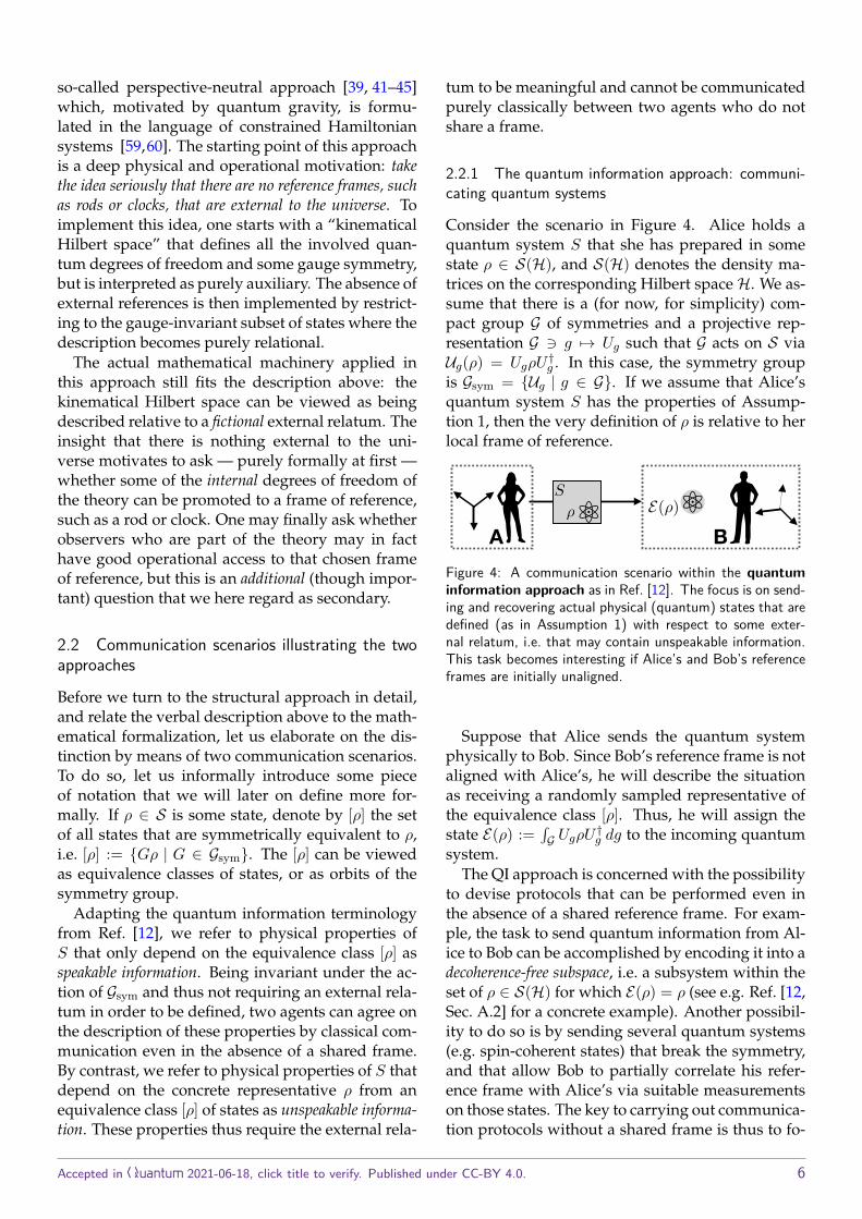
Figure 5: A simple communication scenario which we choosefor illustrating the operational essence of the structural ap-proach as in Refs. [38–40]. The focus is on agents agreeingon a (redundancy-free) description of quantum states in theabsence of an external relatum.

For example, one could imagine the followingcommunication scenario depicted in Figure 5 to il-lustrate the role of “canonical choices”:

• Referee Refaella informs Alice and Bob intheir separate laboratories that she will pre-pare quantum states of a particular system S(subject to Assumption 1) relative to her (freelyaligned) frame, but that she will only commu-nicate the description of the respective equiva-lence classes [ρ] to Alice and Bob separately.


• Alice’s and Bob’s task is to separately return aconcrete (redundancy-free) description of eachquantum state to Refaella and they will win thegame provided their descriptions always agree(either for all states of S, or for a particular classC of states).

• Alice and Bob are only permitted to communi-cate prior to the beginning of the game to agreeon a strategy.

Let us consider two examples for how this can beaccomplished. These examples illustrate that therewill generally exist multiple “canonical choices” fordescribing [ρ] in terms of concrete quantum states,however, that Alice and Bob can always agree intheir communication beforehand which such choiceto pick. This will also give a hint on the rela-tion to quantum reference frames as described inRefs. [38–40], and we will elaborate on this furtherin the following sections.

Example 1. Consider a single quantum spin-1/2 par-ticle, with state space S(C2). Let us assume that thesymmetry group is the full projective unitary group,i.e. Gsym = {ρ 7→ UρU † | U †U = 1}, which is iso-morphic to the rotation group SO(3).

Let ρ be an arbitrary state that Refaella is for somereason interested in preparing. The equivalence class[ρ] consists of all states with the same eigenvaluesλ1, λ2 as ρ. Describing [ρ] is equivalent to listingthe eigenvalues λ1, λ2 and this is what Refaella maycommunicate to Alice and Bob. Clearly, there aremany ways to represent this information in terms ofa concrete quantum state ρ.

The strategy that Alice and Bob can agree on inorder to win the game, but prior to it starting, istrivial: they can agree to always choose a basis (i.e.a specific reference frame alignment) such that ρdescribed relative to it is a diagonal matrix. Thisleaves two “canonical choices” of representation: or-dering the eigenvalues such that λ1 ≥ λ2 they coulddecide to always return either ρ = diag(λ1, λ2) orρ = diag(λ2, λ1) to Refaella. The transformationrelating the two descriptions is the unitary “QRF

transformation” U =(

0 11 0

).

This trivial example relies on the simple fact thatevery quantum state has a canonical description: thematrix representation in its own eigenbasis (up toa choice of order of eigenvalues). In some sense,every quantum state defines a finite set of naturalrepresentations of itself. It is in this sense that thestructural approach interprets quantum systems as

quantum reference frames: the system’s state breaksthe fundamental symmetry, and admits, at least onthe level of classical descriptions, a canonical choiceof representation.

Example 1 illustrates a general consequence ofthe symmetry structure: for any particular choiceof QRF, the set of state descriptions relative to thatQRF corresponds in general only to a subset or sub-space of states. In this example, any such choice onlyallows to describe a subset of states that corresponds toa classical bit: namely, the convex hull of the densitymatrices diag(1, 0) and diag(1/2, 1/2). The follow-ing example demonstrates how a full subspace ofstates can be encoded.

Example 2. Consider two spin -1/2 particles with ro-tational symmetry. That is, the symmetry group isGsym = {ρ 7→ U ⊗ UρU † ⊗ U † | U ∈ SU(2)}, actingon states in S(C2⊗C2). Let us make a somewhat ar-bitrary, but nonetheless illustrative choice of a classC of states for which the above communication gamecan be played. These will be the pure states

C ={

cos θ2 |φ−〉+ eiϕ sin θ2 |φ〉 ⊗ |φ〉}, (1)

where 0 ≤ θ ≤ π, 0 ≤ ϕ < 2π, |φ−〉 is the singletstate, and |φ〉 ∈ C2 an arbitrary normalized state.The set of states C is the disjoint union of the setsCθ,ϕ for which the two angles are fixed and |φ〉 isstill an arbitrary qubit state. Since U ⊗ U |φ−〉 =|φ−〉, the Cθ,ϕ are orbits of the symmetry group, i.e.equivalence classes of states.

If Refaella gives Alice and Bob a description ofsuch an equivalence class [|ψ〉] = Cθ,ϕ, they canagree on returning the standard description |ψ′〉 =cos θ2 |φ−〉+ eiϕ sin θ

2 |0〉 ⊗ |0〉, for example. This pre-scription has the added benefit of preserving super-position across different equivalence classes. Namely,if for i = 1, 2, we have |ψi〉 = αi|φ−〉 + βi|φ〉 ⊗ |φ〉such that |α1| 6= |α2|, then |ψ1〉 and |ψ2〉 are in differ-ent equivalence classes, and so are (in general) theirsuperpositions. But the states that Alice and Bob re-turn respect superpositions: if |ψ〉 = κ|ψ1〉 + λ|ψ2〉,then the returned states satisfy |ψ′〉 = κ|ψ′1〉+ λ|ψ′2〉.That is, this choice of QRF admits the descriptionof a subspace, a qubit, inside the joint state space.Other choices of QRF do so as well. These wouldcorrespond to canonical descriptions where |0〉 ⊗ |0〉is replaced by some arbitrary |φ0〉 ⊗ |φ0〉, and theyare related by “QRF transformations” U ⊗ U .

There are also seemingly natural choices of QRFthat, however, are deficient in that the set of admis-sible descriptions relative to them cannot encom-pass a state space, as the following example illus-trates.


Example 3. Consider again two spin-1/2 parti-cles, but now under slightly different circumstances.There is a canonical choice of factorization of theHilbert space: by looking at the system in isolation,observers can determine the decomposition into twodistinguishable particles. If we assume that this isthe only structure that can be determined by suchobservers, then we have the symmetry group

Gsym = {ρ 7→ (U⊗V )ρ(U †⊗V †) | U †U = V †V = 1}.

Under these circumstances, a canonical choice offrame is such that any pure state |ψ〉 becomes iden-tical to its own Schmidt representation, |ψ〉 =

1∑i=0

√αi|ii〉, where α0 ≥ α1.

While Alice and Bob could easily agree on such aconvention, the ensuing canonical description wouldnot preserve complex superpositions and, in partic-ular, not lead to a subspace of states as its image,owing to the real nature and ordering of the Schmidt-coefficients.

A priori, a choice of QRF in the structural ap-proach can therefore be quite arbitrary. However,as the examples above motivate, a “good” choiceof QRF will correspond to one that admits the de-scription of a set of states relative to it which carriessufficient convex or linear structure to encode clas-sical or quantum information. Preferably, that set ofstates should correspond to a subspace of maximalsize within C.

In the remainder of this article, we will focuson a more interesting realization of such a scenariowhich reproduces the notion of QRFs in the struc-tural picture. We will define particular systems Sthat we call “G-systems”, and we will see that thesecarry an interesting group of symmetries Gsym. If weask what kind of canonical choices of (redundancy-free) description G-systems admit, such that Aliceand Bob can succeed in the communication scenarioof Figure 5, we will find that these correspond tochoosing one of the subsystems of S as a referencesystem and to describing the remaining degrees offreedom relative to it. In this manner, we will re-cover and generalize the “quantum states relative toa particle” of Refs. [38–40]. In particular, the trans-formations among the canonical choices of descrip-tion of S are elements of the symmetry group Gsymand exactly the QRF transformations of Ref. [40],which are also equivalent to the ones in [38, 39] (re-stricted to a discrete setting). In Ref. [72] we willfurther explicitly demonstrate the equivalence withthe perspective-neutral approach to QRFs [39] andelucidate that any equivalence class [ρ] of quantum

states above corresponds precisely to a perspective-neutral quantum state. As we will see, this meansthat the relational states of the structural approachare coherently (not incoherently as in the QI ap-proach) group-averaged states.

3 From symmetries to QRF transforma-tions and invariant observables

Quantum reference frames as described in Refs. [38–40] have first been considered for the case of wavefunctions on the real line. We have a Hilbert spaceof square-integrable functions, H = L2(R), and aphysical claim that there is no absolute notion of ori-gin. In other words, the “physics” does not changeunder translations (we will soon formulate whatthis means in detail). If we have N particles on thereal line, the total Hilbert space is L2(R)⊗N .

As noted in Ref. [40], the real numbers R play adouble role in this case: on the one hand, they la-bel the configuration space on which the wave func-tions are supported; on the other hand, they alsolabel the possible translations, i.e. the fundamentalsymmetry group (R,+).

In this section, we will analyze this particularsituation in a simplified setting: one in which thegroup is finite and Abelian. In the simplest case, wediscretize the real line and make it periodic, as inFigure 1. Formally, for some n ∈ N, we consider thecyclic group

Zn := {0, 1, 2, . . . , n− 1} (2)

with addition modulo n as its group operation. Tothis, we associate a single-particle Hilbert space

H = `2(Zn) = span{|0〉, |1〉, . . . , |n− 1〉} (3)

and a total Hilbert space H⊗N for N distinguish-able particles. We will denote the particles with la-bels A,B,C, . . ., and later in this paper with inte-gers 1, 2, 3, . . .. Within this formalism, we can real-ize the main ideas of quantum references frames asin Refs. [38–40]. For the case N = 2, consider thequantum state

|ψ〉AB = |0〉A ⊗1√2

(|1〉+ |2〉)B . (4)

We are interested in a situation where “only the re-lation between the particles” matters, but not theirtotal position. That is, in some sense, “applying el-ements of Zn to a quantum state doesn’t change the


physics”. Intuitively, this means, for example, thatthe quantum state

|ψ′〉AB = |1〉A ⊗1√2

(|2〉+ |3〉)B (5)

should be an equivalent description of the system’sproperties, since it is related to |ψ〉 by a transla-tion. Motivated by Ref. [38], we can do some-thing more interesting. First, in the terminology ofRefs. [38–40], the form of |ψ〉 can be interpreted assaying that “particle B, as seen by A, is in the state

1√2(|1〉 + |2〉)”. Second, we can then use the pre-

scription of Refs. [38–40] to “jump intoB’s referenceframe”, and consider the state

|ψ′′〉 = 1√2

(|n− 2〉+ |n− 1〉)A ⊗ |0〉B (6)

and conclude that “particleA, as seen byB, is in thestate 1√

2(|n − 1〉 + |n − 2〉)”. After all, this still ex-presses the fact that with amplitudes 1√

2 , B is eitherone or two positions to the right of A.

We will now show that we can understand thesetransformations as natural symmetry transforma-tions in a simple class of physical systems which wecall “G-systems”. Choosing one of the particles as areference frame (as sketched above) will correspondto a choice of canonical representation of a state asin the structural approach outlined above. This willgive the idea of “jumping into a particle’s perspec-tive” a thorough operational interpretation.

3.1 G-systems and their symmetries

We begin by considering a specific physical systemwhich is motivated by translation-invariant quan-tum physics on the real line with Hilbert spaceL2(R). Here we consider a finite, discrete group-theoretic analogue, again using the group as boththe configuration space and set of transformations.Some aspects of QRF transformations in this casewere also considered in Ref. [40]. In contrast toRef. [40], we restrict our attention to finite Abeliangroups G for simplicity. Due to the structure the-orem [73], every such G can be interpreted as thegroup of translations of a discrete torus of some di-mension. In the simplest case where G = Zn, thistorus is the circle2, and we are in the setting of Fig-ure 1.

2This representation is not unique. For example, we caninterpret Z6 as the translation group of six points on a circle,but the structure theorem tells us that Z6 ' Z2 × Z3. Thus,we can also interpret this group as the translations of a two-dimensional (2× 3)-torus.

Definition 4 (G-system). Fix some finite Abeliangroup G, interpreted as a classical configurationspace. That is, we regard the g ∈ G as perfectlydistinguishable orthonormal basis vectors |g〉, span-ning a Hilbert space H. Formally, this Hilbert spaceis H = `2(G), and it carries a distinguished basis{|g〉}g∈G, similarly as quantum mechanics on the realline carries a distinguished position basis.

Consider N distinguishable particles on such aclassical configuration space, where N ∈ N. Thatis, the total Hilbert space is H⊗N , and it carries anatural orthonormal basis

H⊗N = span{|g1, . . . , gN 〉 | gi ∈ G}. (7)

The physical system S described by this Hilbert spacewill carry a group of symmetries Gsym as introducedin Assumption 1 and Figure 3. Clearly, the basicHilbert space structure of S, i.e. the notion of linear-ity and the inner product, must not depend on theorientation of the external reference frame. Hence,the symmetry group will be of the form

Gsym = {U • U † | U ∈ Usym}, (8)

for Usym some group of unitaries. Furthermore, weassume that the classical configuration space, i.e. theset of basis vectors, {|g1, . . . , gN 〉 | gi ∈ G}, is aninternal structure of S that is defined without the ex-ternal reference frame. We now postulate that theclassical configurations carry G-symmetry. In par-ticular, any given configuration

|g〉 := |g1, g2, . . . , gN 〉 (9)

and its “translated” version

U⊗Ng |g〉 = |gg〉 := |gg1, gg2, . . . , ggn〉 (10)

are internally indistinguishable. On the other hand,we postulate that the relation between the particlesis accessible to observers without the external frame.To formalize this, consider some tuple h ∈ GN−1 ofgroup elements, i.e. h = (h1, . . . , hN−1). Any stateof the form

|g, h1g, h2g, . . . , hN−1g〉 =: |g,hg〉 (11)

has the same pairwise relations between its particles,no matter what the state |g〉 of the first particle is.We now define Gsym as the largest possible symme-try group that is compatible with these postulates. Tothis end, Usym must be the group of unitary transfor-mations with the following properties:

1. U maps classical configurations to classical con-figurations, i.e. U |g1, ..., gn〉 = |g′1, ..., g′n〉.


2. On classical configurations, U preserves relativepositions, i.e. U |g,hg〉 = |g′,hg′〉.

3. If two classical configurations are g-translationsof each other, then U preserves this fact, i.e.

|g〉 = U⊗Ng |j〉 ⇒ U |g〉 = U⊗Ng

(U |j〉

). (12)

A few words of justification are in place. Whiletwo choices of external reference frame may yielda different description of any configuration, theymust agree on the set of all possible configurationsthat S can be in, for otherwise their descriptions of Scannot be placed in full relation with one another.3

The set of basis vectors {|g〉}g∈GN must thus be in-dependent of the external frame and hence shouldremain invariant under Gsym. It is also clear that thesymmetry group must preserve the linear and prob-abilistic structure of quantum theory and therebyleave the inner product on H⊗N invariant.4 Af-ter all, by Assumption 1, symmetry related quan-tum states should be indistinguishable even prob-abilistically. Furthermore, the h label the ’relativepositions’ among the N particles. These are inter-nal properties of S and so independent of any ex-ternal relatum. Finally, configurations that are g-translations of each other are by assumption inter-nally indistinguishable. The symmetry group mustpreserve this indistinguishability.

Note that it is possible to drop assumption 3., andto assume only 1. and 2. In this case, one obtainssimilar results to those presented here, but withmodified structures: the algebra of invariant oper-ators then becomes what we call Aalg in Lemma 26,and the symmetry group becomes the group of con-ditional permutations (not only conditional transla-tions). Physically, this does not seem particularlywell-motivated, and it leads to the loss of certainuniqueness results, including the uniqueness of U ∈Usym in Theorem 18.

The symmetry group of a G-system can now eas-ily be written down. To this end, define the sub-spaces

Hh := span{|g,hg〉 | g ∈ G} (13)

3This assumes that the external frame choices in the ambi-ent laboratory that an agent may have access to are completein the sense that all quantum properties of S can be describedrelative to them.

4In constraint quantization, H⊗N corresponds to the kine-matical Hilbert space and so the preservation refers here tothe kinematical inner product. While one is usually only in-terested in the physical inner product (i.e. the inner producton the space of solutions to the constraints), it neverthelessholds that also the kinematical inner product is left invariantby the group generated by the (self-adjoint) constraints.

and the corresponding orthogonal projectors Πh.Note thatH⊗N =

⊕h∈GN−1 Hh, and the {Πh}h∈GN−1

define a projective measurement.

Lemma 5. The symmetry group of a G-system is

Usym =

U =⊕

h∈GN−1

U⊗Ngh

∣∣∣∣∣∣ gh ∈ G

, (14)

where U⊗Nghdenotes the global translation by gh, but

restricted to the subspace Hh.

That is, the symmetries in Usym act as relation-conditional global translations: every classical config-uration is globally translated via some U⊗Ngh

, but theamount of translation gh may depend on the rela-tion h between the particles. We will soon identifythe QRF transformations of Refs. [38–40] with ele-ments of this group. Thus, the above highlights thatthese transformations make sense in a purely clas-sical context; indeed, the corresponding classicalframe transformations were also studied in [39, 40]and shown to be conditional on the interparticle re-lations.5 For example, they can also be applied ifone deals with statistical mixtures of particle posi-tions instead of superpositions. Nonetheless, theirunitary extension to all of H⊗N leads to interestingquantum effects like the frame-dependence of en-tanglement [38–40]. This is similar to the behaviorof the CNOT gate in quantum information theory,which is defined by its classical action on two bits,but nonetheless can create entanglement.

Proof. Due to conditions 1. and 2. of Definition 4,the U ∈ Usym leave every Hh invariant. Thus, Udecomposes into a direct sum U =

⊕h∈GN−1 Uh. Fix

some h ∈ GN−1. Since Hh is invariant, there existssome gh ∈ G such that U |e,h〉 = |gh,hgh〉. Now,for every g ∈ G, we have |g,hg〉 = U⊗Ng |e,h〉. Thus,condition 3. of Definition 4 implies that

U |g,hg〉 = U⊗Ng

(U |e,h〉

)= U⊗Ng |gh,hgh〉

= U⊗Nggh|e,h〉 = U⊗Ngh

|g,hg〉. (15)

This shows that Uh acts like U⊗Nghon Hh.

When working with pure state vectors, we some-times want to allow global phases. Thus, we use thenotation

U∗sym := Usym ×U(1) = {eiθU | U ∈ Usym, θ ∈ R}.

5More precisely, in the perspective-neutral approach theseclassical reference frame transformations correspond to condi-tional gauge transformations, i.e. the gauge flow distance de-pends on the subsystem relations, see Appendix B of Ref. [39]and also Refs. [41–43].


Above, we have decided to denote the state of theparticles relative to the first particle, but this also de-fines the relations between all other pairs of parti-cles: the equation |g〉 = |g,hg〉 ∈ Hh means thatgi = hi−1g1 for i ≥ 2, but this implies that gi =(hi−1h

−1j−1)gj for all i, j if we set h0 := e, the unit el-

ement of the group. Thus, the Hh decompose theglobal Hilbert space into sectors of equal pairwiserelations.

It is clear that global G-translations are elementsof the symmetry group, but they do not exhaust it:

Example 6. Given any G-system, the global trans-lations U⊗Ng are symmetry transformations. Sincethey represent the global action of G on the N -particleHilbert space, this can be written as

G ⊂ Gsym. (16)

However, there are other symmetries that are notglobal translations. For example, for N = 2 parti-cles, the unitary U which acts on all basis vectors|g1, g2〉 as

U |g1, g2〉 := |g2, g−11 g2

2〉 (17)

is a symmetry transformation, i.e. U ∈ Usym.Namely, |g1, g2〉 ∈ Hh for h = g−1

1 g2, and U im-plements the global translation U⊗2

g(h) on Hh, whereg(h) = h.

On the other hand, the transformation

V |g1, g2〉 := |g−12 , g−1

1 〉 (18)

is not a symmetry transformation: it satisfies condi-tions 1. and 2. of Definition 4, but violates condition3.

We will later see that QRF transformations corre-spond to elements in Gsym \ G.

3.2 Invariant observables and Hilbert space de-composition

Which observables can we internally measure in aG-system, i.e. without access to the external relatumthat was used to define the state space and the sym-metry group? These must be the observables thatare invariant under all symmetry transformationsand which thus correspond to speakable informa-tion:

Definition 7 (Invariant observable). We define the in-variant subalgebra Ainv as

Ainv = {A ∈ L(H⊗N ) | [U,A] = 0 for all U ∈ Usym},

where L(H) denotes the set of linear operators onHilbert space H. These are the operators A that are

invariant under all symmetry transformations A 7→UAU †. A self-adjoint element A = A† ∈ Ainv iscalled an invariant observable.

Since all observable properties of our system areassumed to be invariant under Gsym, it follows thatthe observables in Definition 7 comprise the set of allobservables that can be physically measured by anobserver who does not have access to the externalreference frame.

Clearly, all the Πh are invariant observables, i.e.Πh ∈ Ainv. However, due to the fact that we havedeclared a classical basis to be a distinguished struc-ture of the G-system, there are many more invari-ant observables. To determine the algebra Ainv, re-call the decomposition of U ∈ Usym from Lemma 5.We can regard Usym as a representation of severalcopies of the group G, and thus further refine thisdecomposition via basic representation theory of fi-nite Abelian groups [73].

A major role is played by the characters of G. Theseare the homomorphisms χ : G → S1, i.e. the mapsfrom G to the complex unit vectors S1 := {z ∈C, | |z| = 1}with χ(gh) = χ(g)χ(h). In other words,the characters are the one-dimensional irreduciblerepresentations (irreps) of G, and these turn out toexhaust all irreps. The set of all characters of G isdenoted G.

Denote the order of the group by n := |G|, thengn = e for all g ∈ G [73]. Thus, every χ(g) must beamong the n-th roots of unity: χ(g)n = 1. Moreover,there are exactly n characters, i.e. |G| = n.

Furthermore, note that dimHh = n. We claim thatthese subspaces can be decomposed as follows:

Hh =⊕χ∈G

Hh;χ (19)

with Hh;χ the one-dimensional subspace spannedby the vector

|h;χ〉 := 1√|G|

∑g∈G

χ(g−1)|g,hg〉. (20)

Indeed, due to Ref. [73, Proof of Corollary III.2.3],we have the well-known orthogonality relations∑g∈G χ(g)χ′(g) = nδχ,χ′ . Using this, direct cal-

culation shows that the |h;χ〉 are orthonormalizedstates, and

U⊗Ng |h;χ〉 = χ(g)|h;χ〉 for all g ∈ G. (21)

Example 8. As a simple example, consider the cyclicgroup G = Zn = {0, 1, . . . . , n − 1} with additionmodulo n, see Figure 4. This group can be inter-preted as a finite analogue of a part of the real line


with periodic boundary conditions, by distributingfinitely many possible positions along a ring. Its irre-ducible representations and the respective charactersare given by χk(g) := ei

2πnkg with k ∈ {0, 1, . . . , n −

1} [78]. Indeed, one can directly verify that theχk form one-dimensional representations of Zn, andthey are inequivalent. We explicitly obtain

|h;χk〉 = 1√n

n−1∑g=0

e−i2πnkg |g, g + h〉 , (22)

where g+h means that g is added to each componentof h, modulo n. Similarly, one can directly verifythat

U⊗Ng |h;χk〉 = ei2πnkg |h;χk〉 . (23)

One can see that the |h;χk〉 are obtained via a kindof discrete Fourier transform [77] from the classicalconfigurations, and therefore they are reminiscent ofmomentum eigenstates.

Since elements of Usym translate all particles bythe same amount, and momentum is the generator oftranslations, one may identify |h;χk〉 with the eigen-states of total momentum. However, since we arenot explicitly interested in dynamics in this paper,we will postpone any elaboration on this analogy toour upcoming work, Ref. [72].

From Eqs. (14)–(21) it is clear that the subspacespanned by the eigenstates with trivial characterχ = 1 is the subspace of Usym-invariant states, |ψ〉 =U |ψ〉 for all U ∈ Usym. We denote it by

Hphys :=⊕

h∈GN−1

Hh;1 = span{|h; 1〉 | h ∈ GN−1

}.

(24)We have equipped the total invariant subspace withthe label “phys” because it is the finite group ver-sion of the so-called physical Hilbert space of con-straint quantization. When the symmetry group isgenerated by (self-adjoint) constraints, the physicalHilbert space corresponds to the set of solutions tothe quantum constraints and is thereby precisely theHilbert space on which the group acts trivially. Itis usually called ‘physical’ because quantum statesof a gauge system are required to satisfy the con-straints imposed by gauge symmetry. Nevertheless,we will see that we can give quantum states that arenot invariant under the symmetry group a usefulphysical interpretation, and we will clarify their re-lation with the ‘physical’ states inHphys in Ref. [72].Being spanned by the states |h; 1〉which encode theparticle relations in an invariant manner, we shallhenceforth also refer to Hphys as the subspace of re-lational states. Its dimension is |G|N−1, and thus:

Lemma 9. The subspace of relational states Hphys isisomorphic to H⊗(N−1).

To determine the invariant subalgebra, considerany A ∈ L(H⊗N ) and develop it into the |h;χ〉-eigenbasis: A =

∑h,h′,χ,χ′ ah,h′,χ,χ′ |h;χ〉〈h′;χ′|. Us-

ing Eqs. (14) and (21), conjugation with some U ∈Usym yields

UAU † =∑

h,h′,χ,χ′χ(gh)χ′(gh′)−1ah,h′,χ,χ′ |h;χ〉〈h′;χ′|.

This is equal to A for all U if and only if forall h,h′, χ, χ′, one of the following is true: eitherah,h′,χ,χ′ = 0 or χ(gh) = χ′(gh′) for all possiblechoices of gh, gh′ . The latter condition is automat-ically satisfied if χ = χ′ = 1. Thus, all operators Athat are fully supported on the relational subspaceHphys will be elements of Ainv. Let us denote the setof such operators byAphys, then we have just shownthat Aphys ⊂ Ainv. For reasons that will becomeclear later, we will call the observables in Aphys re-lational observables.

Now consider the other cases in which at least oneof χ or χ′ differs from 1. Clearly, if h = h′ and χ = χ′

then the character condition χ(gh) = χ′(gh′) is triv-ially satisfied, and ah,h,χ,χ does not need to be zero.Consider the case h = h′ and χ 6= χ′. Choosing anygh with χ(gh) 6= χ′(gh) shows that we must haveah,h,χ,χ′ = 0. Finally, if h 6= h′ and at least one of χor χ′ (say, χ) differs from 1, choose gh′ = e and ghsuch that χ(gh) 6= 1. This violates the character con-dition and implies ah,h′,χ,χ′ = 0. In summary, wehave proven the following:

Lemma 10. The invariant algebra consists exactly ofthe block matrices of the form

Ainv =

Aphys ⊕⊕

h∈GN−1

⊕χ 6=1

ah;χ|h;χ〉〈h;χ|

,(25)

where Aphys ∈ Aphys is supported on the relationalsubspace Hphys defined in Eq. (24), and the ah;χ arecomplex numbers.

A few words are in place regarding the physicalinterpretation of these observables. Due to Eq. (20),χ labels the irreps of the global translations on statespace. As already mentioned in Example 8, they canthus be interpreted as a discrete analog of (an expo-nentiated version of) total momentum. We can henceinterpret the operator |h;χ〉〈h;χ| as describing aprojective measurement that asks whether the rela-tion between the particles is h, and whether the total mo-mentum corresponds to χ. Since this operator is con-tained in Ainv, this measurement can be performed


by an observer without access to the external ref-erence frame. In the special case if χ = 1, i.e. onthe relational subspace Hphys which corresponds to“total momentum zero”, such an observer can alsoperform measurements that correspond to superpo-sitions of different particle relations h. However, for“non-zero total momentum” (χ 6= 1), we obtain anemergent superselection rule that forbids such su-perpositions and the corresponding measurements.

The reader familiar with constraint quantizationwill notice that the invariant observables Aphys onthe subspace Hphys are the finite group analog ofso-called Dirac observables [29, 30, 59]. Given somecontinuous group that is generated by an algebraof constraints, Dirac observables are operators thatcommute with the constraint operators (up to termsproportional to the constraints themselves). Assuch, they are invariant under the group generatedby the constraints and observables on solutions tothe constraints, i.e. on the so-called physical Hilbertspace.

There is, however, a subtlety in this analogy: usu-ally the (continuous) group generated by the con-straints would be the analog of the ‘classical’ groupG given here which is a strict subgroup of Gsym.Thus, it is natural to ask whether the Gsym-invariantsubspace Hphys is a strict subset of the subspace ofG-invariant states. Accordingly, one may wonderwhether the entire invariant algebra Ainv defined interms of invariance under the larger group Gsym inDefinition 7 is a strict subset of the algebra that isinvariant under the smaller group G. It is this latteralgebra which thus gives rise to the actual analog ofDirac observables for the finite groups consideredhere. We will address these questions in the nextsubsection.

3.3 Group averaging states

Although we work with a representation of thelarger group Gsym, Eqs. (14)–(24) indicate that thetotal Hilbert space decomposes naturally in termsof the representation of the smaller group G; e.g., thephysical Hilbert space is also precisely the subspaceinvariant under G. We will now clarify this obser-vation by considering the corresponding (coherent)group averaging operations,

Πphys := 1|Usym|

∑U∈Usym

U, Π′phys := 1|G|

∑g∈G

U⊗Ng ,

(26)which are standard in constraint quantization [30,61, 62], and for which the following holds.

Lemma 11. The two coherent group averaging oper-ations coincide, Πphys = Π′phys, and Πphys is the or-thogonal projector onto the relational subspace Hphys.

Proof. Direct calculation shows that Π†phys = Πphys

and Π′†phys = Π′phys, and that Π′phys = Π′2phys andΠphys = Π2

phys. Thus, Πphys and Π′phys are orthogo-nal projectors. Since H⊗N is spanned by the |g,hg〉for g ∈ G and h ∈ GN−1, the image im(Π′phys) ofΠ′phys is spanned by

Π′phys |g,hg〉 = 1|G|

∑g′∈G

U⊗Ng′ |g,hg〉 = |h; 1〉√|G|

.(27)

Since these states span Hphys, this proves that Π′physis the orthogonal projector onto the physical sub-space. By construction, every |ψ〉 ∈ im(Πphys) is in-variant under every U ∈ Usym, and thus in particularunder every U⊗Ng ∈ Usym. Thus, im(Πphys) ⊆ Hphys.On the other hand, decomposing U ∈ Usym as in (14),we get

Πphys|h; 1〉 = 1|Usym|

∑U∈Usym

U⊗Ngh|h; 1〉 = |h; 1〉

(28)since |h; 1〉 is invariant under global translations.Thus, im(Πphys) ⊇ Hphys, and so Πphys = Π′phys.

In conclusion, any basis state inHh projects to thesame invariant subnormalized state Πphys |g,hg〉 =Πphys |g′,hg′〉 = 1√

|G||h; 1〉 under coherent group

averaging, and it does not matter whether one av-erages with respect to the larger group Gsym or thesmaller G.

However, we will now see that the set of invari-ant observables, i.e. the observables resulting fromincoherent group averaging (G-twirling), differs forthe two choices, but only outside of the relationalsubspaceHphys. These operations are defined by

Πinv(ρ) := 1|Usym|

∑U∈Usym

UρU †, (29)

Π′inv(ρ) := 1|G|

∑g∈G

U⊗Ng ρ(U⊗Ng )†. (30)

It is well-known, and easy to check by direct cal-culation, that these maps are projectors, i.e. Π2

inv =Πinv and Π′2inv = Π′inv, and that they are orthogonalwith respect to the Hilbert-Schmidt inner product,i.e. for all A,B ∈ L(H⊗N ),

tr(A†Πinv(B)

)= tr

(Πinv(A)†B

). (31)

If A ∈ L(H⊗N ) satisfies [U,A] = 0 for all U ∈ Usym,then Πinv(A) = A. Conversely, if B ∈ im(Πinv), then


UBU † = B, i.e. [U,B] = 0, for all U ∈ Usym. Thus,Πinv projects into the invariant algebra Ainv. Simi-larly, Π′inv projects into

A′inv = {A ∈ L(H⊗N ) | [U⊗Ng , A] = 0 for all g ∈ G}.

Clearly, Ainv ⊆ A′inv, but are these algebras equal?The following lemma collects the above insights,and answers this question in the negative.

Theorem 12. Πinv is the orthogonal projector ontothe invariant subalgebra Ainv. It can also be writtenin the form

Πinv(ρ) = ΠphysρΠphys+∑

h,χ 6=1〈h;χ|ρ|h;χ〉|h;χ〉〈h;χ|.

Similarly, Π′inv is the orthogonal projector onto thestrictly larger subalgebra

A′inv =

⊕χ∈G

Aχ

=

Aphys ⊕⊕χ 6=1

Aχ

, (32)

where every Aχ is an arbitrary operator supported onthe subspace Hχ := span{|h;χ〉 | h ∈ GN−1} (notethat H1 = Hphys, so Aphys = A1).

Proof. To see the claimed form of Πinv, note thatthe combination of projections is a Hilbert-Schmidt-orthogonal projection with image Ainv. It remains tobe shown that A′inv has the claimed form. Note thatg 7→ U⊗Ng is a representation of the finite Abeliangroup G. It thus decomposes into one-dimensionalirreps, and the equivalence classes of irreps are la-belled by the characters χ. Thus, the form of A′invfollows again from Schur’s lemma.

This theorem has interesting implications for thephysical properties of G-systems S. Recall our ini-tial scenario as depicted in Figure 3. Suppose thatwe only demand symmetry of S with respect to ordi-nary, unconditional global translations U⊗Ng , and askwhich observables can be measured by an observerwithout access to the external relatum. The answeris: all observables in A′inv. On the other hand, ifwe demand symmetry with respect to all conditionalglobal translations in Usym — and we will soon seethat the QRF transformations of Refs. [38–40] areamong those — then this turns out to be a morestringent requirement. In this case, fewer observ-ables are measurable, namely only those in Ainv.

In this sense, QRF transformations have fewerframe-independent observables than classical trans-formations: if all QRF transformations are symme-tries, then superpositions of different particle rela-tions h are forbidden by an emergent superselec-tion rule whenever the “total momentum is non-zero”, i.e. χ 6= 1. On the other hand, if we only

demand that global classical translations are sym-metries, then these superpositions remain allowed.

Let us return to the analogy with contraintquantization discussed in the previous subsection.Lemma 11 and Theorem 12 show that an observ-able Aphys, i.e. the analog of a Dirac observable inour context, does not depend on whether it is con-structed relative to Gsym or its subgroup G. Later,we will also see that Aphys is the finite group ana-log of the algebra generated by so-called relationalDirac observables. These are invariant observablesthat encode relations between the subsystems, andthey are common use in canonical quantum grav-ity [29–37,42–45]. This explains why we have calledthe observables in Aphys “relational observables”.They will become crucial in the resolution of theparadox of the third particle in Section 4, and theywill turn out to be tomographically complete for theQRF states which we introduce in the next subsec-tion.

Recall the notion of equivalence classes [ρ] fromSection 2. We are now ready to introduce this notionformally for G-systems:

Definition 13. We call two quantum states ρ, σ ∈S(H⊗N ) symmetry-equivalent, and write ρ ' σ, ifthere exists some symmetry U ∈ Usym such thatσ = UρU †. We call them observationally equivalent,and write ρ ∼ σ, if tr(Aρ) = tr(Aσ) for all invariantobservables (and thus all operators) A ∈ Ainv.

Clearly, if ρ ' σ then ρ ∼ σ, but the converse isnot in general true. The equivalence class [ρ] fromSection 2 can now be defined as [ρ] = {σ | σ ' ρ}.In the case of pure state vectors |ψ〉, |ψ′〉, we mustallow global phases and write ψ ' ψ′ if and only ifthere is some U ∈ U∗sym such that |ψ′〉 = U |ψ〉.

Observational equivalence can be characterizedin terms of the projection into the invariant subal-gebra:

Lemma 14. Two states ρ and σ are observationallyequivalent, i.e. ρ ∼ σ, if and only if

Πinv(ρ) = Πinv(σ). (33)

Proof. This follows from the chain of equivalences

ρ ∼ σ⇔ 〈A, ρ〉HS = 〈A, σ〉HS ∀A ∈ Ainv

⇔ 〈Πinv(B), ρ〉HS = 〈Πinv(B), σ〉HS ∀B ∈ L(H⊗N )⇔ 〈B,Πinv(ρ)〉HS = 〈B,Πinv(σ)〉HS ∀B ∈ L(H⊗N )⇔ Πinv(ρ) = Πinv(σ).


3.4 Alignable states as states with a canonical rep-resentation

With these technical insights at hand, we are readyto return to the discussion of Section 2. In thestructural approach to QRFs, we ask whether agiven state has a natural representation, depend-ing only on internal data, such that the communi-cation task of Figure 5 can be successfully accom-plished. In the following, let us focus on pure states|ψ〉 ∈ H⊗N for simplicity. Our task is to find an-other state |ψ′〉 ∈ H⊗N that is symmetry-equivalentto |ψ〉 and that is in some sense distinguished, i.e.yields a “canonical choice” for describing the set ofsymmetry-equivalent states, cf. Section 2.2.2.

In general, there may be many different possibleways to define such a “canonical choice”. Let uspick one possible choice. Suppose that we fix oneof the particles, say, particle i, where 1 ≤ i ≤ N .Can we set the external reference frame such thatthis particle ends up at the “origin” — the unit ele-ment of the group? In other words, can we align ourstate “relative to particle i”? This is certainly pos-sible in classical mechanics of N point particles inone dimension, given translation-invariance. Clas-sically, it would indeed define us a unique represen-tation. We will now see that a similar constructioncan be done for G-systems, and that it leads to thenotion of QRF of Refs. [38, 40].

Definition 15. Let i ∈ {1, 2, . . . , N}. A pure state|ψ〉 ∈ H⊗N is called i-alignable if there exists somestate |ψ′〉 ∈ H⊗N with ψ ' ψ′ such that

|ψ′〉 ≡ |ψ′〉1,...,N = |e〉i ⊗ |ϕ〉1,...,i−1,i+1,...,N . (34)

In the following, we will also use the notation |ϕ〉ifor the vector |ϕ〉1,...,i−1,i+1,...,N .

The state |ϕ〉i in Definition 15 is exactly what is in-terpreted in Refs. [38–40] as “the state of the remain-ing N − 1 particles as seen by particle i”. Similarly,we will thus interpret |e〉i⊗|ϕ〉i as the description ofthe N particle system relative to the QRF ‘perspec-tive’ defined by particle i (which defines the origin).

Not all pure states are i-alignable. For exam-ple, the relational state |h; 1〉 is an element of thesubspace Hphys, hence every U ∈ U∗sym satisfiesU |h; 1〉 = eiθ|h; 1〉 for some θ ∈ R. Thus this statecannot be i-alignable for any i. While devoid ofalignable states, we will see later that Hphys con-tains the complete relational information about allalignable states.

To analyze this notion further, the followinglemma will be useful.

Lemma 16. For every i ∈ {1, . . . , N} and h ∈ GN−1,there is a unique basis vector |g〉 ∈ Hh with gi = g,namely |h−1

i−1g,hh−1i−1g〉, with h0 := e the unit ele-

ment of G.

Proof. If |g〉 ∈ Hh then |g〉 = |l,hl〉 for some l ∈ G.Hence gi = hi−1l which is equal to g if and only ifl = h−1

i−1g.

This allows us to show that the state |ψ′〉 in Defini-tion 15 is unique, and thus defines indeed a naturalrepresentation of the symmetry-equivalence class of|ψ〉:

Lemma 17. If |ψ〉 ∈ H⊗N is i-alignable, then thestate |ϕ〉i in Definition 15 is unique up to a globalphase.

Proof. Suppose that both ψ′ and ψ′ are states thatsatisfy the conditions of Definition 15. In particular,this means that ψ ' ψ′ and ψ ' ψ′, and so thereexists some U ∈ U∗sym such that |ψ′〉 = U |ψ′〉, andU = eiθV for V ∈ Usym. In |ψ′〉 = |e〉i ⊗ |ϕ〉i and|ψ′〉 = |e〉i⊗|ϕ〉i, we decompose ϕ and ϕ into productbasis vectors: |ϕ〉 =

∑g∈GN−1 αg|g1, . . . , gN−1〉, and

similarly for |ϕ〉 with amplitudes αg. This impliesthat

U∑

g∈GN−1

αg|g1, . . . , gi−1, e, gi, . . . , gN−1〉

=∑

g∈GN−1

αg|g1, . . . , gi−1, e, gi, . . . , gN−1〉. (35)

Now, according to Lemma 16, both of the decompo-sitions

∑g∈GN−1 . . . contain at most one basis vec-

tor from every subspace Hh with non-zero ampli-tude, namely |h−1

i−1,hh−1i−1〉. But since U (and thus

V ) leaves the subspaces Hh invariant, the last equa-tion implies that V |h−1

i−1,hh−1i−1〉 = |h−1

i−1,hh−1i−1〉 for

every such vector that appears with non-zero ampli-tude αg 6= 0 (and thus αg 6= 0). Hence αg = e−iθαg,and so ϕ = e−iθϕ.

3.5 QRF transformations as symmetry group ele-ments

In the structural approach in Refs. [38–40], we can“jump” from one particle’s reference frame into anyother’s. How is this idea expressed in our formal-ism? To see this, let us first show the following.

Theorem 18 (QRF state transformations). If thereis some i ∈ {1, 2, . . . , N} such that |ψ〉 is i-alignable,then |ψ〉 is j-alignable for every j ∈ {1, 2, . . . , N}.We will then simply call |ψ〉 alignable. Moreover, forevery i, j ∈ {1, . . . , N}, there is a unique symmetrytransformation U ∈ Usym such that U (|e〉i ⊗ |ϕ〉i) =


|e〉j⊗|ϕ〉j for all |ϕ〉i. Furthermore, if i 6= j then U isa proper conditional global translation, i.e. U •U † ∈Gsym \ G. Every such U induces a unique unitary(“QRF transformation”) Vi→j such that Vi→j |ϕ〉i =|ϕ〉j. This transformation can be written

Vi→j = Fi,j∑g∈G|g−1〉〈g|j ⊗ U⊗(N−2)

g−1 , (36)

where Fi,j flips (swaps) particles i and j. This is thediscrete version of the form given in Refs. [38, 40].Proof. Fix i, j ∈ {1, . . . , N}. For every h ∈ GN−1,let gh := h−1

j−1hi−1 (setting, as before, h0 := e). Thenthe global translation by gh satisfies

U⊗Ngh|h−1i−1,hh

−1i−1〉 = |h−1

j−1,hh−1j−1〉. (37)

Set U :=⊕

h∈GN−1 U⊗Ngh, then U ∈ Usym. According

to Lemma 16, for every h, U maps the unique basisvector |g〉 ∈ Hh with gi = e to the unique basisvector |g′〉 ∈ Hh with g′j = e, and it is clear that Uis the only symmetry transformation that does this.Thus, U maps all states of the form |e〉i ⊗ |ϕ〉i tostates of the form |e〉j ⊗ |ϕ〉j . Furthermore, if i 6= jthen there exist h, j such that gh 6= gj. Thus, anysuch U is an h-dependent transformation and thuscannot be a global translation.

Fix an arbitrary orthonormal basis {|ϕ〉i}ϕ ofH⊗(N−1), then U (|e〉i ⊗ |ϕ〉i) = |e〉j⊗|ϕ〉j yields an-other orthonormal basis. Thus, we can view this asa unitary Vi→j from H⊗(N−1) into another copy ofH⊗(N−1). Since its action on basis vectors is fixed,there can be no more than one such map. To deter-mine that it has the form as claimed, simply look atits action on the basis vectors |g1, . . . , gN−1〉.

So indeed, for every alignable state, and any par-ticle j ∈ {1, . . . , N}, there is a unique representationof that state “relative to the jth particle”. Further-more, the QRF transformation from i’s to j’s ‘per-spective’ at the level of the full Hilbert space H⊗Ncorresponds to a symmetry transformation whichlies in Gsym, but not in G (if i 6= j). This observa-tion highlights the physical significance of the sym-metry group Gsym. While we have seen that the setof invariant states Hphys is independent of whetherone constructs it through coherently averaging overGsym or its ‘classical translation subgroup’ G, thesymmetry group Gsym is key for understanding themeaning of the QRF transformations (which trans-form non-invariant descriptions): they are condi-tional symmetry transformations that depend on theinterparticle relation h.

To clarify the notation used in the definition of theQRF transformation Vi→j , we give a simple exam-ple.

Example 19. Suppose we have N = 4 particles, andan alignable state |ψ〉 such that

|ψ〉 ' |e〉2 ⊗ |g1, g3, g4〉. (38)

Thus, the state relative to the second particle is|g1, g3, g4〉. To determine the state relative to thethird particle, compute

V2→3|g1, g3, g4〉 = F2,3∑g∈G|g−1〉〈g|3 ⊗ U⊗2

g−1 |g1, g3, g4〉

= F2,3|g−13 〉〈g3| ⊗ U⊗2

g−13|g1, g3, g4〉

= F2,3| g−13 g1︸︷︷︸

1

, g−13︸︷︷︸3

, g−13 g4︸︷︷︸

4

〉

= | g−13 g1︸︷︷︸

1

, g−13︸︷︷︸2

, g−13 g4︸︷︷︸

4

〉, (39)

where the integers at the bottom denote the particlelabels.

In Ref. [72], we will demonstrate equivalence ofthe above QRF transformations with the “quantumcoordinate changes” of the perspective-neutral ap-proach [39, 41–45].

As Theorem 18 has shown, the symmetry groupUsym contains the QRF transformations whichswitch from state descriptions relative to particle ito descriptions relative to particle j. But these donot exhaust the symmetry group. The followinglemma gives another physically motivated exam-ple.

Example 20 (Center of mass). Consider again thecyclic group Zn with addition modulo n, as shownin Figure 1. Let m1, . . . ,mN be non-negative realnumbers and m := m1 + . . . + mN . For h ∈ GN−1,define the group elements

g(h) := −⌊ 1m

(m2h1 + . . .+mNhN−1)⌋, (40)

and set U :=⊕

h∈GN−1 U⊗Ng(h). If we interpret the mi

as the masses of the particles, with the origin as theposition of particle 1 (i.e. h0 = 0), then this symme-try transformation U describes a change of quantumcoordinates such that the (integer part of) the “centerof mass” becomes the origin.

3.6 Characterization of alignable states

We have already seen that not all global states arealignable. The following lemma characterizes thosethat are.


Lemma 21. A state |ψ〉 ∈ H⊗N is alignable if andonly if it can be written in the form

|ψ〉 =∑

h∈GN−1

αh|gh,h gh〉 (41)

for some gh ∈ G and αh ∈ C. Moreover, theαh characterize the alignable state up to symmetry-equivalence. That is, for two alignable states |ψ〉 and|ψ′〉, we have ψ ' ψ′ if and only if their coefficientssatisfy αh = eiθα′h for some θ ∈ R.

Proof. If |ψ〉 is alignable, then it is in particular 1-alignable. That is, there exists U ∈ U∗sym such that

|ψ〉 = U(|e〉1 ⊗ |ϕ〉1

)= eiθ

∑h∈GN−1

αhU⊗Ngh|e,h〉,

where the αh are the coefficients of |ϕ〉1 in termsof the product group basis, and the U⊗Ngh

translatethe basis vectors of the subspaces Hh. Hence we getthe claimed form for |ψ〉. The converse direction ofthe proof of the first part of this lemma is analo-gous. We also see that the αh only depend on thesymmetry-equivalence class of the state |ψ〉 (up to aglobal phase); and, in the case of equality of thosecoefficients, two states must have the same |ϕ〉1 (upto a global phase), hence they must be symmetry-equivalent.

The above form shows that any maximal sub-space of H⊗N which is contained in the set ofalignable states has dimension |G|N−1, i.e. is isomor-phic to H⊗(N−1). This shows that the QRFs as de-fined above are indeed “good” QRFs as explainedin Subsection 2.2.2. Due to Lemma 9, it also showsthat the relational subspace Hphys has the right di-mension for its states to contain “all the particles’internal QRF perspectives at once”. This observa-tion is corroborated by the following useful Lemmaand will be further discussed in Ref. [72].

Lemma 22. Given any alignable state |ψ〉 (which ishence of the form (41)), its projection onto the in-variant subalgebra is

Πinv(|ψ〉〈ψ|) (42)

=∑

h,j∈GN−1

αhαj|G||h; 1〉〈j; 1|+

∑h∈GN−1

|αh|2

|G|Πh;χ 6=1,

where Πh;χ 6=1 :=∑χ 6=1 |h;χ〉〈h;χ|. Thus, for any

two alignable states |ψ〉, |ψ′〉, we have ψ ∼ ψ′ ifand only if ψ ' ψ′: such states are symmetry-equivalent if and only if they are observationallyequivalent. Furthermore, they are equivalent if andonly if 〈ψ|A|ψ〉 = 〈ψ′|A|ψ′〉 for all A ∈ Aphys; that is,all invariant information of alignable states is fullycontained in their projection Πphys|ψ〉.

Proof. Using (27), we obtain

Πphys|ψ〉 = 1√|G|

∑h∈GN−1

αh|h; 1〉. (43)

Direct calculation shows that |〈ψ|h;χ〉|2 = |αh|2/|G|.The result then follows by using the form of Πinv asgiven in Theorem 12. Both notions of equivalenceboil down to the fact that the states have the sameamplitudes αh up to a global phase. Finally, for ρany alignable state, the above form of Πinv(ρ) implies

tr(ρA) (44)= tr(ρphysA) +

∑h∈GN−1

〈h; 1|ρphys|h; 1〉tr(Πh;χ 6=1A)

for all A ∈ Ainv, where ρphys := ΠphysρΠphys. Thatis, the expectation values of all invariant observables,and thus the notion of observational equivalence, de-pends only on the state’s projection into Aphys.

In other words, the algebra Aphys is tomograph-ically complete for the invariant information inalignable states. In this sense, it can be said thatthe external relatum independent states of the struc-tural approach are what we called the relationalstates, namely the ones in Hphys. That is, the ex-ternal relatum independent states of the structuralapproach are the coherently group-averaged states,while their counterparts in the QI approach arethe incoherently group-averaged states (cf. Subsec-tion 2.2.1).6

3.7 Alignable and relational observables

Given the notion of alignable states and the dualitybetween states and observables, it is natural to alsodefine alignable observables in the obvious way.

Definition 23 (Alignable observables). An operatorA ∈ L(H⊗N ) is called i-alignable for i ∈ {1, . . . , N}if there exists U ∈ Usym such that

UAU † = |e〉〈e|i ⊗Ai (45)

for some Ai ∈ L(H⊗(N−1)). If A is an observable, itis called an i-alignable observable.

This leads to the following extension of Theo-rem 18 from QRF state to observable transforma-tions. The proof is analogous and thus omitted.

Theorem 24 (QRF observable transformations). IfA ∈ L(H⊗N ) is i-alignable, then it is also j-alignablefor every j ∈ {1, . . . , N}, and so we will call A simply

6We thank A. R. H. Smith for suggesting us to emphasizethis technical distinction.


alignable. In particular, there is a unique U ∈ Usymsuch that

U (|e〉〈e|i ⊗Ai)U† = |e〉〈e|j ⊗Aj , (46)

where Aj = Vi→j Ai Vj→i. Here, U is the uniquesymmetry transformation from Theorem 18 such thatU (|e〉i ⊗ |ϕ〉i) = |e〉j ⊗ |ϕ〉j for all |ϕ〉i and Vi→j isthe unitary “QRF transformation” induced by it.

These are the discrete versions of the observabletransformations in Refs. [38, 39].

Finally, note that if A1 =∑

h,j∈GN−1 ah,j|h〉〈j|,then

Πphys(|e〉〈e|1 ⊗A1

)=

∑h,j∈GN−1

ah,j|G||h; 1〉〈j; 1|,

(47)where Πphys henceforth denotes the superoperatorthat acts as Πphys(A) = ΠphysAΠphys, as obviousfrom Lemma 22. Up to a factor of |G|, this is identicalto the original representation of A1, but in anotherbasis. This proves the following theorem, extendinga result from [44, 45]:

Theorem 25. Consider the map

Ai 7→ FAi,i := |G| · Πphys(|e〉〈e|i ⊗Ai

), (48)

where Ai ∈ L(H⊗(N−1)) is any operator. This de-fines an isomorphism between the operators Ai andAphys, preserving products, linear combinations, andadjoints.

This gives us two independent motivations to fo-cus onAphys: for alignable states, the projection intothis subalgebra contains all invariant information;and it does so in a way that preserves the naturalstructure of the alignable observables.

Furthermore, returning to the comparison withconstraint quantization, it follows from Refs. [44,45]that FAi,i is (the finite group analog of) the relationalDirac observable which encodes in an invariant man-ner the question “what is the value of Ai given thatparticle i sits at the origin?” Such relational observ-ables are a standard tool in canonical quantum grav-ity, e.g. see Refs. [29–37, 42, 43]. Theorem 25 is thereason why we refer to Aphys as the algebra gener-ated by relational observables.

Due to Aphys ⊂ Ainv, we have

Πphys (Πinv(|e〉〈e|i ⊗Ai)) = Πphys (|e〉〈e|i ⊗Ai) .

Since Πinv is the incoherent G-twirl over Usym, it isclear that the image Πinv(|e〉〈e|i ⊗ Ai) ∈ Ainv onlydepends on the symmetry equivalence class of the

alignable observable A. Hence, in particular wehave

FAi,i = FAj ,j for all i, j ∈ {1, . . . , N}, (49)and so the relational observable in Eq. (48) does notdepend on the choice of particle i.

This systematic equivalence of relational observ-ables is once more made possible by studying thelarger symmetry group Gsym rather than its sub-group G as usual in the literature. Indeed, Theo-rems 18 and 24 demonstrate that any two particlealignments of an observable are related by a uniquesymmetry group element which generically lies inGsym \ G.

Lemma 22 (and its obvious generalization toalignable observables) yields an interesting insightthat will become relevant in Section 4: if we lookat the image of all alignable states and observablesunder Πinv, then we do not obtain the full invariantalgebraAinv. Instead, we always obtain an operatorin the smaller subalgebra

Aalg :=

Aphys +∑

h∈GN−1

ahΠh;χ 6=1

, (50)

where Aphys ∈ Aphys, and ah ∈ C are arbitrary com-plex numbers. According to the definitions in Sub-section 3.3, this gives us the subalgebra inclusions

Aphys ⊂ Aalg ⊂ Ainv ⊂ A′inv ⊂ L(H⊗N ). (51)

Hence, if we denote the orthogonal projection intoAalg by Πalg, we have Πalg◦Πinv = Πinv◦Πalg = Πalg.More specifically, the following holds.

Lemma 26. Aalg is the smallest subalgebra ofL(H⊗N ) that contains Πinv(|ψ〉〈ψ|) for all alignablestates |ψ〉.Proof. It is clear that the rank-one projectors |ψ〉〈ψ|for |ψ〉 = |e〉1 ⊗ |ϕ〉1 linearly span all of |e〉〈e|1 ⊗L(H⊗(N−1)), thus we are looking for the subalgebraA that is generated by the image of these operatorsunder Πinv. Lemma 22 shows that Πinv(|ψ〉〈ψ|) iscontained in Aalg for every alignable state |ψ〉, henceA ⊆ Aalg. Conversely, if A =

∑h,j∈GN−1 ah,j|h〉〈j|,

then

Πinv(|e〉〈e| ⊗A) (52)

=∑

h,j∈GN−1

ah,j|G||h; 1〉〈j; 1|+

∑h∈GN−1

ah,h|G|

Πh;χ 6=1.

Setting A := |h〉〈j| for h 6= j shows that|h; 1〉〈j; 1| ∈ A. But then, we also have |h; 1〉〈h; 1| =|h; 1〉〈j; 1|)(|j; 1〉〈h; 1|) ∈ A, and so all operatorsAphys fully supported on Hphys are in A. Finally,considering the image of A = |h; 1〉〈h; 1| shows thatΠh;χ 6=1 ∈ A, and so A ⊇ Aalg.


3.8 Communication scenario of the structural ap-proach revisited

We are now in a position to revisit the communi-cation scenario elucidating the operational essenceof the structural approach to QRFs in section 2.2.2(see also Figure 5). It is clear how Alice and Bobcan win the game proposed by Refaella in the caseof N particles on the configuration space G in theabsence of a shared external relatum, given thatthe class of states C that they are interested in isthe set of alignable states. For example, before thegame begins, they can agree to always use particle1 as the internal reference system relative to whichthe remaining particles are described. This yieldsthe “canonical choice” to represent any equivalenceclass of (pure) states in the form |e〉1 ⊗ |ϕ〉1 and Al-ice’s and Bob’s return to Refaella will always agree.

Alice and Bob have, of course, the option tochoose any of the N particles as a reference sys-tem, each likewise defining a “canonical choice”. Itis clear that all these different possible conventionsby Alice and Bob are precisely related by the QRFtransformations of Lemma 18 and that each suchtransformation is an element of the symmetry groupUsym.

4 The paradox of the third particle andthe relational trace

Ref. [50] presents a “paradox of the third particle”in the context of QRFs. We will now formulate thisapparent paradox in our formalism, and see that thestructure of observables, as elaborated in Section 3,helps to clarify its physical background and to re-solve it in terms of relational observables. As wewill see, the core of the problem is how to embedthe two-particle observables into the set of three-particle observables, and the key will be to do so ina relational manner. This bears some resemblanceto the issue of boundaries and edge modes in gaugetheory and gravity [64–71], which is related to thequestion of how to embed the gauge-invariant ob-servables of neighbouring subregions in spacetimeinto the set of gauge-invariant observables associ-ated with the union (‘gluing’) of these subregions.

The setup of Ref. [50] consists of three particles inone dimension, i.e. on the real line R. But since onlya finite number of positions is relevant for the para-dox, we can discretize space and its translations.Thus, we consider a G-system with G = Zn, thecyclic group of order n, as in Fig. 1. The group oper-ation is addition modulo n; in the following, when-

ever we write a+ b, we actually mean a+ b mod n.As described earlier, this is a discrete model of thetranslation group acting on the real line. We startwith two particles that have been prepared (by anexternal observer with access to the reference frame)in the state

|ψ〉 = 1√2

(| − a〉1|b〉2 + eiθ|a〉1| − b〉2

), (53)

where a, b ∈ {0, 1, 2, . . . , n−1}, and θ ∈ R. This stateis symmetry-equivalent to7

|ψ〉 ' |0〉1 ⊗1√2

(|a+ b〉2 + eiθ| − a− b〉2

). (54)

In our terminology, this means that the state isalignable. In Ref. [50], this form is used as a mo-tivation to declare: “Therefore, we conclude that par-ticle 1 sees particle 2 in a pure state. Importantly thisimplies that particle 1 can get access to the phase θ by in-teracting with particle 2 alone, i.e. without access to theexternal reference frame.” In our conceptual frame-work, we would rather describe the situation as fol-lows: consider an external observer who has accessto particles 1 and 2, but has no access to the externalreference frame. There are some observables thatthis observer can measure for which the phase θ isrelevant.

This is because the state that is effectively seen bythis observer is the projection of ψ into the invariantsubalgebra, which we can determine via Lemma 22.The coefficients of this state are αh = 1/

√2 for h =

a+ b and αj = eiθ/√

2 for j = −a− b, thus

Πinv(|ψ〉〈ψ|) = 12n |h; 1〉〈h; 1|+ e−iθ

2n |h; 1〉〈 j; 1|

+eiθ

2n |j; 1〉〈h; 1|+ 12n |j; 1〉〈j; 1|

+ 12nΠh;χ 6=1 + 1

2nΠj;χ 6=1 (55)

and this state depends on θ in a nontrivial way.Now a third particle is introduced. From the

external perspective, it is prepared in a pure state|c〉 independently of the other two particles, wherec ∈ {0, 1, . . . , n − 1}. From that perspective, theglobal state thus reads

|Ψ〉 = 1√2

(| − a〉1|b〉2 + eiθ|a〉1| − b〉2

)|c〉3. (56)

This state is still alignable. Relative to particle 1, itbecomes

|Ψ′〉 = |0〉1√2(|a+ b〉2|a+ c〉3 + eiθ| − a− b〉2| − a+ c〉3

)(57)

7In fact, in the sequel we will assume that a 6= 0, for oth-erwise the states in Eqs. (53) and (54) coincide.


with Ψ′ ' Ψ. This is a state for which particles 2and 3 are formally entangled. Now suppose thatparticle 3 is very far away, such that our externalobserver (or, as the authors of Ref. [50] would say,such that particle 1) has no access to particle 3. Ifone now formally takes the partial trace over parti-cle 3, one obtains a reduced state of particles 1 and2 that is independent of the phase θ. This seems to con-tradict our earlier claim — now it looks as if an ex-ternal observer without access to the external refer-ence frame or to particle 3 cannot see any observableconsequences of the phase θ.

We arrive at an apparent paradox: computingthe partial trace via Ψ or via Ψ′ gives different pre-dictions, even though both states are symmetry-equivalent. Moreover, the result from tracing outthe third particle via Ψ′ seems absurd, given theseemingly innocuous role that the third particleplays in state Ψ. Can the phase θ be accessed byan observer without access to the external relatumand with restricted access to only particles 1 and 2?It seems like there should be an objective answer tothis question which does not depend on whether itis asked in the context of state Ψ or Ψ′.

Clearly, since the usual partial trace yields differ-ing results for Ψ and Ψ′, it cannot represent the cor-rect rule to compute reduced states in the setting ofQRFs. To shed light on the reason for why this isthe case, let us reconsider how the standard partialtrace can be motivated. Consider three distinguish-able particles as one usually does in quantum infor-mation theory — in our setting, this implies that thestate of the particles is defined relative to an acces-sible reference frame. Denote by A12 some observ-able that is measurable if one has access to particles1 and 2 only (and to the reference frame). Then onecan equivalently describe this as an observable onthe three particles, such that the third particle is ig-nored. Formally, this can be done via a map

A12 7→ Φ(A12) = A12 ⊗ 13. (58)

That is, the 2-particle observables are naturally em-bedded into the 3-particle observables via somemap Φ, which takes the tensor product with theidentity observable. This map preserves all relevantstructure (as it must): it takes linear combinations tolinear combinations, products to products, the ad-joint to the adjoint, and the identity to the identity.Formally, this is summarized by saying that Φ isa unital ∗-homomorphism. It defines what we meanwhen we talk about “observables pertaining onlyto particles 1 and 2” within the set of all 3-particleobservables. In the following, we will refer to ∗-homomorphisms simply as embeddings (which may

or may not be unital).Now consider any quantum state ρ123 on the three

particles. We would like to determine the state ρ12that results if one has only access to particles 1 and2. By this, we mean the state that gives the sameexpectation values as ρ123 on all local observablesA12. Thus, we demand

tr(ρ12A12) = tr(ρ123Φ(A12)) for all A12. (59)

If we write this in terms of the Hilbert-Schmidt in-ner product, then

〈ρ12, A12〉HS = 〈ρ123,Φ(A12)〉HS = 〈Φ†(ρ123), A12〉HS.

That is, we must have ρ12 = Φ†(ρ123), with Φ† theHilbert-Schmidt adjoint of Φ. But given Eq. (58), itis easy to see that Φ† = Tr3, and this recovers thepartial trace.

In the context of QRFs and G-systems, we have adifferent structure of observables: what is measur-able without access to the external reference framecorresponds to the invariant observables. We there-fore need an analog of the above construction forthe invariant subalgebra Ainv. In fact, since we areonly interested in alignable states, Lemma 26 tellsus that we can focus on the subalgebra Aalg.

4.1 The non-uniqueness of invariant embeddings

In light of the above considerations, let us try toconstruct an embedding of the relevant 2-particleobservables (or more generally of A(N)

alg ) into the 3-

particle observables (more generally into A(N+M)alg ,

where the superscript denotes the number of parti-cles). To obtain some crucial physical intuition, wewill now define one such embedding (called Φ(1)) inan intuitive manner, before we turn to a more sys-tematic treatment below.

We start our construction with the orthogonalprojector Π(N)

h :=∑χ∈G |h;χ〉〈h;χ|. Its embedding

must be on orthogonal projector in A(N+M)alg ; mea-

suring this projector amounts to asking whether thefirst N particles have pairwise relations describedby h. Clearly, the answer must be “yes” wheneverthe M +N particles are in some joint relation (h,g)for arbitrary g ∈ GM , and the answer must be “no”for all other relations (h′,g) whenever h′ 6= h. Thissuggests to choose the embedding as

Φ(1)(Π(N)h ) =

∑g∈GM

Π(N+M)h,g . (60)

The reason for the superscript ‘(1)’ will becomeclear shortly. Now consider the orthogonal pro-jector Π(N)

phys :=∑

h∈GN−1 |h; 1〉〈h; 1|. A state |ψ〉


is in the image of this projector if and only if itis translation-invariant, i.e. U⊗Ng |ψ〉 = |ψ〉 for allg ∈ G. Suppose that a state of N + M particlesis translation-invariant; then we would like to beable to say that the state of the first N particles istranslation-invariant, too. This motivates us to de-mand Φ(1)(Π(N)

phys) = Π(N+M)phys : in other words, we

embed the translation-invariant observables of Nparticles into the translation-invariant observablesof N +M particles.

We have |h; 1〉〈h; 1| = Π(N)h Π(N)

phys. Since Φ(1) issupposed to be an embedding and thus multiplica-tive, this implies

Φ(1)(|h; 1〉〈h; 1|) =∑

g∈GM|h,g; 1〉〈h; g; 1|. (61)

To exhaust all of A(N)alg , we still need to embed the

operators |h; 1〉〈j; 1| for h 6= j. Given Eq. (61), itseems formally natural to define

Φ(1)(|h; 1〉〈j; 1|) :=∑

g∈GM|h,g; 1〉〈j,g; 1|. (62)

Natural as this definition may seem, we will soonsee that it relies on quite subtle physical assump-tions. For now, let us work with this definitionand explore its consequences. First, linearity andEqs. (60) and (61) imply

Φ(1) (Πh,χ 6=1)

=∑

g∈GMΠh,g;χ 6=1. (63)

These demands yield an embedding that can equiv-alently be defined as follows:

Lemma 27. There is a unique unital embedding Φ(1)

of A(N)alg into A(N+M)

alg that satisfies

Φ(1)(Π(N)

alg (e1 ⊗A1))

= Π(N+M)alg

(e1 ⊗A1 ⊗ 1(M)

)(64)

for all A1 ∈ L(H⊗(N−1)), where e1 := |e〉〈e|1 and1 := {2, 3, . . . , N}. It is given by the linear extensionof Eqs. (62) and (63).

Proof. Write A1 =∑

h,j∈GN−1 ah,j|h〉〈j| and useLemma 22 to obtain

Π(N)alg (|e〉〈e|1 ⊗A1) =

∑h,j∈GN−1

ah,j|G||h; 1〉〈j; 1|

+∑

h∈GN−1

ah,h|G|

Πh;χ 6=1. (65)

A similar representation can be obtained for theright-hand side of Eq. (64). Thus, it is clear thatthe linear extension of Eqs. (62) and (63) satisfiesEq. (64). In particular, the unit is preserved.

Now let Φ be any embedding of A(N)alg into A(N+M)

algwhich satisfies Eq. (64). Choose h, j ∈ GN−1 arbi-trary, and let A1 be the operator with ah,j = |G|and all other coefficients zero. Then Eq. (65) be-comes |h; 1〉〈j; 1|, and Π(N+M)

alg

(|e〉〈e|1 ⊗A1 ⊗ 1(M)

)becomes the right-hand side of Eq. (62). Now, stillfor h 6= j,

(|h; 1〉〈j; 1|)† (|h; 1〉〈j; 1|) = |j; 1〉〈j; 1|. (66)

Since Φ preserves adjoints and products, this provesEq. (62) also in the case h = j. Finally, choosing A1such that ah,h = |G| and all other coefficients zeroproves Eq. (63), which implies that Φ is the linearextension of Eqs. (62) and (63).

What this lemma demonstrates is that our con-struction of Φ(1) can be interpreted in an alternativeway — at least on “alignable” observables. Whatour embedding map does to those observables is asfollows: write them in the form |e〉〈e|1⊗A1, and embedthem into the total Hilbert space according to its definingtensor product structure. Then demand that Φ(1) mapsthe invariant part of |e〉〈e|1 ⊗ A1 to the invariant partof its embedding |e〉〈e|1 ⊗ A1 ⊗ 1(M). This defines aparticular, natural embedding ofA(N)

alg intoA(N+M)alg .

But this suggests directly that our candidate re-lational trace is defective: its definition is implicitlybased on the choice of particle 1 as our reference. Indeed,the following lemma shows that there is a large classof invariant embeddings. In particular, choosing an-other particle as the reference particle will in generallead to inequivalent embeddings. The proof is givenby a straightforward calculation and thus omitted.

Lemma 28. Let U ∈ Usym be any symmetry transfor-mation (for example, a QRF transformation). Thenthere is a unique unital embedding ΦU of A(N)

alg intoA(N+M)

alg which satisfies

ΦU(

Π(N)alg (e1 ⊗A1)

)= Π(N+M)

alg

(U(e1 ⊗A1)U† ⊗ 1(M)

).

(67)Writing U =

⊕h∈GN−1 U⊗Ng(h), it acts as

ΦU (|h; 1〉〈j; 1|)=

∑g∈GM

|h, g(h)−1g; 1〉〈j, g(j)−1g; 1|, (68)

ΦU (Πh;χ 6=1)

=∑

g∈GNΠh,g;χ 6=1. (69)

Via ΦU := ΦU ◦ Π(N)alg , this extends to a completely

positive unital map ΦU : L(H⊗N )→ L(H⊗(N+M)).


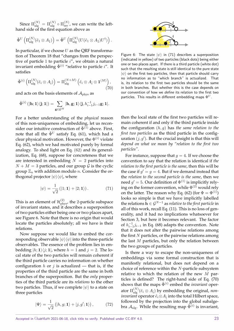
Since Π(N)alg = Π(N)

alg ◦ Π(N)inv , we can write the left-

hand side of the first equation above as

ΦU(Π(N)

alg (e1 ⊗A1))

= ΦU(Π(N)

alg (U(e1 ⊗A1)U †)).

In particular, if we choose U as the QRF transforma-tion of Theorem 18 that “changes from the perspec-tive of particle 1 to particle i”, we obtain a naturalinvariant embedding Φ(i) “relative to particle i”. Itsatisfies

Φ(i)(Π(N)

alg (ei ⊗Ai))

= Π(N+M)alg

(ei ⊗Ai ⊗ 1(M)

),

(70)and acts on the basis elements of Aphys as

Φ(i) (|h; 1〉〈j; 1|) =∑

g∈GM|h,g; 1〉〈j, h−1

i−1ji−1g; 1|.

For a better understanding of the physical reasonof this non-uniqueness of embedding, let us recon-sider our intuitive construction of Φ(1) above. First,note that all the ΦU satisfy Eq. (61), which had aclear physical motivation. However, the Φ(i) violateEq. (62), which we had motivated purely by formalanalogy. To shed light on Eq. (62) and its general-ization, Eq. (68), suppose for concreteness that weare interested in embedding N = 2 particles intoN + M = 3 particles, and our group G is the cyclicgroup Zn with addition modulo n. Consider the or-thogonal projector |ψ〉〈ψ|, where

|ψ〉 = 1√2

(|1; 1〉+ |2; 1〉) . (71)

This is an element of H(2)phys, the 2-particle subspace

of invariant states, and it describes a superpositionof two particles either being one or two places apart,see Figure 6. Note that there is no origin that wouldlocate the particles absolutely; all we have is theirrelations.

Now suppose we would like to embed the cor-responding observable |ψ〉〈ψ| into the three-particleobservables. The essence of the problem lies in em-bedding |h; 1〉〈j; 1|, where h = 1 and j = 2. The lo-cal state of the two particles will remain coherent ifthe third particle carries no information on whetherconfiguration h or j is actualized — that is, if theproperties of the third particle are the same in bothbranches of the superposition. But the only proper-ties of the third particle are its relations to the othertwo particles. Thus, if we complete |ψ〉 to a state onthree particles

|Ψ〉 = 1√2(|h, g; 1〉+ |j, g′; 1〉

), (72)

<latexit sha1_base64="E4OBzma/mXr/7pCSIX+7mj4IFVY=">AAAB6XicbVA9SwNBEJ2LXzF+RS1tFoNgFe40oIVFwMYyAWMCyRH2NnPJmr29Y3dPCEd+gY2Fgtj6j+z8N26SKzTxwcDjvRlm5gWJ4Nq47rdTWFvf2Nwqbpd2dvf2D8qHRw86ThXDFotFrDoB1Si4xJbhRmAnUUijQGA7GN/O/PYTKs1jeW8mCfoRHUoeckaNlZqX/XLFrbpzkFXi5aQCORr98ldvELM0QmmYoFp3PTcxfkaV4UzgtNRLNSaUjekQu5ZKGqH2s/mhU3JmlQEJY2VLGjJXf09kNNJ6EgW2M6JmpJe9mfif101NeO1nXCapQckWi8JUEBOT2ddkwBUyIyaWUKa4vZWwEVWUGZtNyYbgLb+8StoXVa9W9bxmrVK/yfMowgmcwjl4cAV1uIMGtIABwjO8wpvz6Lw4787HorXg5DPH8AfO5w8Rsozq</latexit>

3

<latexit sha1_base64="VRrXuKP0vCNvWlHGiYhkNcT0k5A=">AAAB6XicbVA9SwNBEJ2LXzF+RS1tFoNgFe5CQAuLgI1lAsYEkiPsbeaSNXt7x+6eEI78AhsLBbH1H9n5b9wkV2jig4HHezPMzAsSwbVx3W+nsLG5tb1T3C3t7R8cHpWPTx50nCqGbRaLWHUDqlFwiW3DjcBuopBGgcBOMLmd+50nVJrH8t5ME/QjOpI85IwaK7Vqg3LFrboLkHXi5aQCOZqD8ld/GLM0QmmYoFr3PDcxfkaV4UzgrNRPNSaUTegIe5ZKGqH2s8WhM3JhlSEJY2VLGrJQf09kNNJ6GgW2M6JmrFe9ufif10tNeO1nXCapQcmWi8JUEBOT+ddkyBUyI6aWUKa4vZWwMVWUGZtNyYbgrb68Tjq1qlevel6rXmnc5HkU4QzO4RI8uIIG3EET2sAA4Rle4c15dF6cd+dj2Vpw8plT+APn8wcQLYzp</latexit>

2

<latexit sha1_base64="lGqFEdu+Zvlv/I8uFf5ae8a7mSQ=">AAAB5XicbVBNS8NAEJ3Urxq/qlcvi0XwVBIp6MFDwYvHCsYW2lA220m7drMJuxuhhP4CLx4UvPqXvPlv3LY5aOuDgcd7M8zMizLBtfG8b6eysbm1vVPddff2Dw6Pau7xo05zxTBgqUhVN6IaBZcYGG4EdjOFNIkEdqLJ7dzvPKPSPJUPZpphmNCR5DFn1Fjpvjmo1b2GtwBZJ35J6lCiPah99YcpyxOUhgmqdc/3MhMWVBnOBM7cfq4xo2xCR9izVNIEdVgsDp2Rc6sMSZwqW9KQhfp7oqCJ1tMksp0JNWO96s3F/7xebuLrsOAyyw1KtlwU54KYlMy/JkOukBkxtYQyxe2thI2poszYbFwbgr/68jrpXDb8ZsP3662bMo0qnMIZXIAPV9CCO2hDAAwQXuAN3p0n59X5WDZWnHLiBP7A+fwBp9uLwA==</latexit>

4

<latexit sha1_base64="lGqFEdu+Zvlv/I8uFf5ae8a7mSQ=">AAAB5XicbVBNS8NAEJ3Urxq/qlcvi0XwVBIp6MFDwYvHCsYW2lA220m7drMJuxuhhP4CLx4UvPqXvPlv3LY5aOuDgcd7M8zMizLBtfG8b6eysbm1vVPddff2Dw6Pau7xo05zxTBgqUhVN6IaBZcYGG4EdjOFNIkEdqLJ7dzvPKPSPJUPZpphmNCR5DFn1Fjpvjmo1b2GtwBZJ35J6lCiPah99YcpyxOUhgmqdc/3MhMWVBnOBM7cfq4xo2xCR9izVNIEdVgsDp2Rc6sMSZwqW9KQhfp7oqCJ1tMksp0JNWO96s3F/7xebuLrsOAyyw1KtlwU54KYlMy/JkOukBkxtYQyxe2thI2poszYbFwbgr/68jrpXDb8ZsP3662bMo0qnMIZXIAPV9CCO2hDAAwQXuAN3p0n59X5WDZWnHLiBP7A+fwBp9uLwA==</latexit>

4

Figure 6: The state |ψ〉 in (71) describes a superposition(indicated in yellow) of two particles (black dots) being eitherone or two places apart. If there is a third particle (white dot)such that the resulting state is still identical to the pure state|ψ〉 on the first two particles, then that particle should carryno information as to “which branch” is actualized. Thatis, its relation to the first two particles should be the samein both branches. But whether this is the case depends onour convention of how we define its relation to the first twoparticles. This results in different embedding maps ΦU .

then the local state of the first two particles will re-main coherent if and only if the third particle insidethe configuration (h, g) has the same relation to thefirst two particles as the third particle in the config-uration (j, g′). But the crucial insight is that this willdepend on what we mean by “relation to the first twoparticles”.

For instance, suppose that g = 4. If we choose theconvention to say that the relation is identical if therelation to the first particle is the same, then this will bethe case if g′ = g = 4. But if we demand instead thatthe relation to the second particle is the same, then weneed g′ = 5. Our definition of Φ(1) is implicitly rely-ing on the former convention, while Φ(2) would relyon the latter. The reason why Eq. (62) (for Φ = Φ(1))looks so simple is that we have implicitly labelledthe relations h ∈ GN−1 as relative to the first particle inall of this work, recall Eq. (11). This is no loss of gen-erality, and it had no implications whatsoever forSection 3, but here it becomes relevant. The factorof h−1

i−1ji−1 in Eq. (68) adapts the convention. Notethat it does not alter the pairwise relations amongthe firstN particles, or the pairwise relations amongthe last M particles, but only the relation betweenthe two groups of particles.

Is there a way to escape the non-uniqueness ofembeddings via some formal construction that ismanifestly relational, but does not depend on achoice of reference within the N -particle subsystemrelative to which the relation of the new M par-ticles is defined? The right-hand side of Eq. (70)shows that the maps Φ(i) embed the invariant oper-ator Π(N)

alg (ei ⊗ Ai) by embedding the original, non-invariant operator ei⊗Ai into the total Hilbert space,followed by the projection into the global subalge-bra Aalg. While the resulting map Φ(i) is invariant,


its definition is therefore not. Can we perhaps makethe definition invariant by embedding not ei⊗Ai di-rectly, but its invariant part? The following lemmaanswers this question in the negative:

Lemma 29. Define the map Φ : A(N)alg → A

(N+M)alg as

Φ(A(N)) := Π(N+M)alg

(A(N) ⊗ 1(M)

). (73)

Then this map is not a valid embedding. Namely, itis not in general multiplicative, i.e. there exist A,B ∈A(N)

alg with Φ(AB) 6= Φ(A)Φ(B).

Proof. A tedious but straightforward calculationyields

Φ (|h; 1〉〈j; 1|) = 1|G|

∑g∈G

∑g∈GM

|h,g; 1〉〈j, gg; 1|

+ 1|G|

δh,j∑

g∈GMΠh,g;χ 6=1. (74)

But then, for h 6= j, we obtain

Φ(|h; 1〉〈j; 1|)Φ(|j; 1〉〈h; 1|) 6= Φ(|h; 1〉〈h; 1|).

A similar argument applies if we try to embedA(N)

inv intoA(N+M)inv : the analog of the above construc-

tion, with Π(N+M)alg replaced by Π(N+M)

inv , does notyield a valid embedding.

4.2 A class of invariant traces

For every embedding ΦU of Lemma 28, we obtain acorresponding “invariant trace”:

Lemma 30. For every U =⊕

h∈GN−1 U⊗Ng(h) ∈ Usym,define a corresponding “invariant trace” TrinvU :=(ΦU)†

. It is trace-preserving, and it maps invari-ant operators to invariant operators. In particular,TrinvU(M)

(A(N+M)

alg

)= A(N)

alg , and can be explicitlywritten in the following form:

TrinvU(M) ρ =∑

h,j∈GN−1

|h; 1〉〈j; 1|∑

g∈GM〈h, g(h)−1g; 1|ρ|j, g(j)−1g; 1〉+

∑h∈GN−1

Πh;χ 6=1∑

g∈GM

tr(Πh,g;χ 6=1ρ)|G| − 1 .

We omit the straightforward proof.Since the different invariant traces formalize dif-

ferent ways to embed the two-particle observablesinto the three-particle observables, it is clear thatthe answer to the question raised at the beginningof this section will depend on the embedding. Inother words, the question of whether the phase θis accessible on the first two particles depends onthe operational definition of how to access the firsttwo particles within the total three-particle Hilbertspace.

To illustrate this fact, let us apply two differentinvariant traces to the paradox. In contrast to theusual partial trace, every invariant trace yields iden-tical results when applied to the equivalent states Ψand Ψ′ in Eqs. (56) and (57) (hence the name “invari-ant”). That is,

TrinvU3 |Ψ〉〈Ψ| = TrinvU3 |Ψ′〉〈Ψ′| (75)

for all U ∈ Usym. However, different U yield dif-ferent results. For example, consider the invarianttrace Trinv1 which is the adjoint of the embeddingΦ(1) that we have constructed in Subsection 4.1. A

straightforward calculation gives

Trinv13 |Ψ〉〈Ψ| =

12n |h; 1〉〈h; 1|+ 1

2n |j; 1〉〈j; 1|

+ 12nΠh;χ 6=1 + 1

2nΠj;χ 6=1

= Π(2)inv

[|e〉〈e|1 ⊗

(12 |h〉〈h|+

12 |j〉〈j|

)2

],

Up to observational equivalence, we hence get amixed state

Trinv13 |Ψ〉〈Ψ| ∼ |e〉〈e|1 ⊗

(12 |h〉〈h|+

12 |j〉〈j|

)2.

In particular, the phase θ has disappeared. This isnot surprising: ultimately, Trinv1 amounts to tak-ing the usual partial trace in the representation ofthe state relative to particle 1, i.e. of the state |Ψ′〉 ofEq. (57).

On the other hand, consider the symmetry trans-formation U from Example 20 which transforms tothe center of mass. Like in Ref. [50], let us choosem1 and m2 such that m1a = m2b. Using Lemma 30,It is clear that

TrinvU3(Πh;χ 6=1

)= Πh1;χ 6=1 (76)


and similarly for h replaced by j. Furthermore,

TrinvU3 (|l; 1〉〈p; 1|) =∑

h,j∈Zn|h; 1〉〈j; 1|

∑g∈Zn〈h, g +

⌊m2mh

⌋; 1|l; 1〉〈p; 1|j, g +

⌊m2mj

⌋; 1〉

= |l1; 1〉〈p1; 1|δl2−bm2ml1c,p2−b

m2mp1c (77)

for all l,p ∈ Z2n. Since TrinvU3 |Ψ〉〈Ψ| =

TrinvU3 (Πalg(|Ψ〉〈Ψ|)), we can expand Πalg(|Ψ〉〈Ψ|)into basis elements and apply the above equations.As a result, this yields exactly Eq. (55) (since a is aninteger, it turns out that we can ignore all b·c). Thatis,

TrinvU3(|Ψ〉〈Ψ|

)= Πinv

(|ψ〉〈ψ|

)∼ |ψ〉〈ψ|. (78)

That is, up to observational equivalence, we ob-tain the original pure alignable state |ψ〉 of Eq. (53).Moreover, in this observational equivalence class,|ψ〉 is unique up to symmetry equivalence: namely,if there is another pure alignable state |ψ′〉 withTrinvU3 (|Ψ〉〈Ψ|) ∼ |ψ′〉〈ψ′|, then ψ ∼ ψ′. But dueto Lemma 22, this implies that ψ ' ψ′. Thus, in par-ticular, there is (up to a global phase) a unique rep-resentation of this state relative to the i-th particle,|ψ〉 ' |e〉i ⊗ |ϕ〉i. According to Eq. (54), it is

|ϕ〉1 = 1√2

(|a+ b〉2 + eiθ| − a− b〉2

)(79)

relative to the first particle. Thus, under the “cen-ter of mass” relational trace TrinvU , the phase θ sur-vives, in contrast to the result for Trinv1.

4.3 Definition of the relational trace

Recalling the invariant algebra inclusions Aphys ⊂Aalg ⊂ Ainv, we have thus far focused on construct-ing an invariant trace for Aalg, since by Lemma 26,it is the smallest algebra containing the invariantpart of all alignable states and observables. How-ever, in the previous subsection, we have seen thatthere does not exist a unique invariant trace on it,and the same conclusion applies to Ainv. We willnow show that, by contrast, there does exists a nat-ural embedding of the algebra A(N)

phys of relational

N -particle operators into the algebra A(N+M)phys of re-

lational (N + M)-particle operators. This will alsolead to a natural definition of an invariant trace interms of relational states.

This trace, which we hence call the relational trace,has a natural and simple definition that is mani-festly invariant under relative translations between

the two particle groups. It is therefore independentof the various physically distinct conventions dis-cussed in the previous subsections. On the rela-tional subspace Hphys, the paradox is therefore un-ambiguously resolved. It is sufficient to focus onthis subspace because Lemma 22 tells us that the re-lational observables are tomographically completefor the invariant information in all alignable states.Thus, Hphys contains all the information we are in-terested in.

Lemma 31. The map Φphys : A(N)phys → A

(N+M)phys , de-

fined by

Φphys(A(N)phys) := Π(N+M)

phys

(A

(N)phys ⊗ 1(M)

)(80)

is an embedding. It simplifies to

Φphys(A(N)phys) = A

(N)phys ⊗Π(M)

phys, (81)

but it is not unital.

Recall that this construction does not yield an em-bedding of all invariant observables A(N)

inv , or evenof A(N)

alg , as we have seen in Lemma 29. Thus, it isremarkable that it works for the subalgebra of rela-tional observables.

Proof. Noting that every A(N)phys ∈ A

(N)phys satisfies

A(N)phys = Π(N)

phys(A(N)phys), we can recast Φphys in the

form

Φphys(A(N)phys) = Π(N+M)

phys

(Π(N)

phys ⊗ 1(M)) (A

(N)phys ⊗ 1(M)

)×(Π(N)

phys ⊗ 1(M))

Π(N+M)phys .

By considering the action on an arbitrary basis state|g1, . . . , gN+M 〉, it is easy to verify that(

Π(N)phys ⊗ 1(M)

)Π(N+M)

phys = Π(N)phys ⊗Π(M)

phys. (82)

Hence, using idempotence of the projector,

Φphys(A(N)phys) = A

(N)phys ⊗Π(M)

phys, (83)

and the image commutes with Π(N+M)phys . Check-

ing the embedding properties is now trivial. Fur-thermore, note that the unit element of A(N)

phys isΠ(N)

phys, while the unit element of A(N+M)phys is Π(N+M)

phys .


However, Φphys(Π(N)phys) = Π(N)

phys ⊗ Π(M)phys. To see

that Φphys(Π(N)phys) does not act as the identity on

H(N+M)phys , observe that tr

(Π(N)

phys

)= dimH(N)

phys =

|G|N−1, hence tr(Π(N)

phys ⊗Π(M)phys

)= |G|N+M−2, but

tr(Π(N+M)

phys

)= |G|N+M−1.

Returning to the discussion of how to define therelations of the additional M particles to the firstgroup of N particles (cf. Fig. 6), we now have aunique answer: the projector Π(M)

phys in Φphys takesthe coherent average over all possible such relations.This can also be seen by inspecting the action ofΦphys on the basis elements of Aphys:

Φphys (|h; 1〉〈j; 1|) = 1|G|

∑g∈G,g∈GM

|h,g; 1〉〈j, gg; 1|.

In contrast to Eq. (72) and the embeddings of Sub-section 4.1, this embedding does not assign to everyM -particle configuration g another one, g′, whichhas “the same relation” to the first N particles inbranches h and j. Instead, it generates the uniformsuperposition of all the possibilities.

This averaging is also the reason for the failureof the unitality property. However, as we will seeshortly, the absence of unitality is precisely the rea-son why the relational trace defined below maps re-lational (N + M)-particle states into relational N -particle states. It will thus be rather a feature than afailure.

While Φphys is not unital, note that the embed-ding of the relational N -particle unit Φphys(Π(N)

phys) =Π(N)

phys ⊗Π(M)phys certainly does act as the identity on its

image,

H(N⊗M)phys :=

{Π(N)

phys ⊗Π(M)phys |ψ〉

∣∣∣ |ψ〉 ∈ H⊗(N+M)}.

This subspace of the space of relational (N + M)-particle statesH(N+M)

phys will be essential below whenresolving the paradox of the third particle.

The natural embedding induces a natural trace.

Definition 32 (Relational trace). The relational traceis defined to be the Hilbert-Schmidt adjoint Trel :=Φ†phys of the extended embedding map Φphys :L(H⊗N )→ L(H⊗(N+M)) defined by Φphys := Φphys ◦Π(N)

phys. That is, the relational trace is the unique mapwith the property

tr(Φphys(A(N)) ρ

)= tr

(A(N) Trel(M)ρ

)(84)

for all A(N) ∈ L(H⊗N ) and all ρ ∈ L(H⊗(N+M)) (inparticular for all states).

Specifically, note that

tr(Φphys(A(N)) ρ

)= tr

(Φphys(A(N)) Π(N+M)

phys (ρ))

= tr(Φphys(A(N)) ρphys

). (85)

This is precisely the expectation value of the rela-tional observable Φphys(A(N)) ∈ A(N+M)

phys in the re-

lational state ρphys ∈ S(H(N+M)phys ), evaluated in the

manifestly invariant inner product on S(H(N+M)phys ).

The relational trace is thus unambiguously definedin terms of the so-called physical inner productof constraint quantization [30, 61, 62], i.e. the innerproduct on Hphys. We will analyze this in more de-tail in our upcoming work [72].

Theorem 33. The relational trace takes the explicitform

Trel(M)ρ = Tr(M)[Π(N)

phys ⊗Π(M)phys ρΠ(N)

phys ⊗Π(M)phys

],

where Tr(M) is the standard partial trace overparticles N + 1, . . . , N + M . It maps rela-tional operators onto relational operators, i.e.Trel(M)

(A(N+M)

phys

)= A(N)

phys, and is trace-preserving

for states in S(H(N⊗M)phys ), but trace-decreasing out-

side of it. Furthermore, it preserves observationalequivalence, i.e. ρ ∼ σ implies Trel(M)ρ = Trel(M)σ.

Proof. The first statement follows from

tr(Φphys(A(N)) ρ

)= tr

[(Π(N)

physA(N)Π(N)

phys ⊗Π(M)phys

)ρ]

= tr[(A(N) ⊗ 1(M)

) (Π(N)

phys ⊗Π(M)phys ρΠ(N)

phys ⊗Π(M)phys

)],

which holds for any A(N) ∈ L(H⊗N ) and any ρ ∈L(H⊗(N+M)).

Given the conjugation of its input with the pro-jector Π(N)

phys⊗Π(M)phys, it is clear that Trel(M) is trace-

preserving for states in S(H(N⊗M)phys ), but not for

states outside of it. It is also clear that Trel(M) mapsoperators fromA(N+M)

phys into operators inA(N)phys, since

the projectors Π(N)phys can be taken outside of the

trace over particles N + 1, . . . , N + M . To seethat it is surjective, it is straightforward to checkthat |G|1−MTrel(M)

(A

(N)phys ⊗ 1(M)

)= A

(N)phys for all

A(N)phys ∈ A

(N)phys.

Finally, note that the image of Φphys is containedin A(N+M)

phys , thus Φphys = Π(N+M)phys ◦ Φphys. Taking

the Hilbert-Schmidt adjoint of this equation yieldsTrel(M) ◦ Π(N+M)

phys = Trel(M). Now suppose we haveρ ∼ σ, then Lemma 14 and Π(N+M)

phys ◦ Π(N+M)inv =

Π(N+M)phys imply Π(N+M)

phys (ρ) = Π(N+M)phys (σ). Alto-

gether this implies that Trel(M) preserves observa-tional equivalence.


We can write

Trel(M) = Π(N)phys ◦ Tr(M) ◦ Π(N+M)

phys . (86)

We can thus view the relational partial trace Trel(M)as an invariant extension of the standard partialtrace Tr(M). The non-unitality of Φphys is reflected

in the final application of Π(N)phys. Without this pro-

jection, the image of Trel(M) would not in general be

contained in A(N)phys. For example, the uniform mix-

ture ρ(N+M) := Π(N+M)phys /|G|N+M−1 on the physical

subspace of N + M particles yields Tr(M)ρ(N+M) =

1(N)/|G|N , whose decomposition according to The-orem 12 contains operators outside of A(N)

phys.8 Thus,

non-unitality is the price to pay for remaining relational.This leads to Trel(M) being trace-decreasing, unless

the initial state is fully supported on the subspaceH(N⊗M)

phys . Should we be worried about this fact —shouldn’t marginals of normalized quantum statesbe normalized? Not in this case. In contrast to thestandard partial trace, the relational trace is not sup-posed to tell us what the reduced quantum state ona subsystem is. Instead, it is constructed to tell usprecisely the following:

Theorem 34. Given some (N + M)-particle stateρ(N+M) ∈ S(H⊗(N+M)), the following conditionalstate of N particles is normalized or subnormalized:

ρ(N) :=Trel(M)ρ

(N+M)

tr(ρ(N+M)Π(N+M)

phys

) . (87)

Consider any relational projector 0 ≤ E(N)phys ≤ Π(N)

physwhich we interpret as a “relational event”. Then thestate ρ(N) tells us the probabilities of this N -particleevent, conditioned on the (N + M)-particle systembeing relational:

tr(E

(N)physρ

(N))

= Prob(E

(N)phys| Π(N+M)

phys

). (88)

That is, the renormalized result ρ(N) of the rela-tional trace gives us the expectation values of allN -particle relational observables, conditioned onthe global (N + M)-particle state being fully rela-tional.

8More generally, the image of H(N+M)phys \ H(N⊗M)

phys underTr(M) does not lie in the N -particle relational subspace H(N)

phys.

Proof. It follows from Theorem 33 and Eq. (82) that

tr(Trel(M)ρ

(N+M))

= tr(Π(N)

phys ⊗Π(M)physρ

(N+M))

≤ tr(Π(N+M)

phys ρ(N+M)), (89)

hence ρ(N) is not supernormalized. Now, the proba-bility that an initial global measurement of the pro-jector Π(N+M)

phys yields outcome “yes”, and then a sub-sequent local measurement of E(N)

phys yields “yes” too,is

Prob(E

(N)phys,Π

(N+M)phys

)= tr

(Φphys(E(N)

phys)Π(N+M)phys (ρ(N+M))

)= tr

(E

(N)physTrel(M) ◦ Π(N+M)

phys (ρ(N+M)))

= tr(E

(N)physTrel(M)ρ

(N+M)), (90)

where we have used Definition 32 and Eq. (86). Therest of the claim follows from the definition of con-ditional probability.

Recall that in Lemma 22, we have seen that theprojection ρphys := Π(N+M)

phys (ρ) for alignable statesρ is subnormalized, but is sufficient to determinethe expectation values of all invariant observables.Thus, ρphys should not be seen as the marginal of ρon some subsystem, but as the “relational part” ofρ. The “relational weight” tr ρphys is in general lessthan one,9 and it can decrease when disregarding

9This assumes that ρ ∈ L(H⊗(N+M)) in ρphys = Π(N+M)phys (ρ)

is normalized, as appropriate in the context of our manuscriptwhere there is an external observer who could measure alsonon-invariant observables in the presence of an external frame.By contrast, in the perspective-neutral approach [39, 41–45](and more generally in constraint quantization), one disregardsany external structure and works directly with normalized re-lational states. That is, one would define the normalization ofthe (N + M)-particle relational state as trρphys = 1. Indeed,note that the full standard trace trρphys = tr

(Π(N+M)

phys ρ)

isprecisely the extension of the so-called physical inner prod-uct [30, 61, 62] to density matrices. However, note also fromthe previous footnote that the standard partial trace Tr(M) isnot in general appropriate for relational states ρphys. The ad-ditional projection with Π(N)

phys in the relational trace fixes thisissue, but reduces the norm of states with support outside ofH(N⊗M)

phys . This has a transparent physical interpretation whichis best seen through the norm reduction of invariant basisstates: Trel(M)(|hN,hM; 1〉〈jN, jM; 1|), where hN , jN ∈ GN−1

and hM , jM ∈ GM , is equal to 1|G| |hN ; 1〉〈jN ; 1| if hM = gjM

for some g ∈ G, and is zero otherwise. The variables hM , jMlying in GM rather than GM−1 reflects the fact that they en-code not only the M − 1 internal relations of the M particles,but also a definite relation between the two particle groups,which is a property of both groups together. The normaliza-tion reduction factor 1/|G| comes from the coherent averagingover the relations between the two particle groups (which ispartially a property of the N particles), and quantifies thecorresponding ignorance of the relational N -particle state ob-


some of the particles.

4.4 Relational resolution of the paradox

In order to apply these insights to the paradox ofthe third particle, let us first discuss some furtheraspects of the interplay of composition and rela-tional trace, for the generic case of M + N parti-cles. Suppose ρ(N) is a state of the N particles be-fore taking the additional M particles into account,prepared by an observer with access to the externalreference frame. The corresponding relational stateis ρ(N)

phys = Π(N)phys(ρ(N)). Next, suppose the M addi-

tional particles are prepared in a normalized stateρ(M), and the composite state of all particles is ofthe product form ρ(N+M) = ρ(N) ⊗ ρ(M). We canthen construct the relational state corresponding tothis composition. Here it is important to note thatρ

(N+M)phys = Π(N+M)

phys

(ρ(N+M)

)= Π(N+M)

phys

(ρ(N+M)

),

for any ρ(N+M) ' ρ(N+M). That is, all membersof the symmetry equivalence class of ρ(N+M) (incl.states featuring entanglement between the two par-ticle groups) yield the same relational (N + M)-particle state. However, due to Theorem 33, it isonly the projection intoH(N⊗M)

phys that matters for therelational trace. But Eq. (82) implies that

Π(N)phys ⊗Π(M)

phys ρ(N+M)phys Π(N)

phys ⊗Π(M)phys

= Π(N)phys ⊗Π(M)

phys

(ρ(N) ⊗ ρ(M)

)Π(N)

phys ⊗Π(M)phys

= ρ(N)phys ⊗ ρ

(M)phys, (91)

and so we have Trel(M)ρ(N+M)phys = ρ

(N)phys · tr(M)ρ

(M)phys.

Up to a constant factor, this is precisely the initialrelational N -particle state that we had before takingthe additional M particles into account.

Let us see what this implies for the paradox of thethird particle. Thus, let us concretely compute therelational trace Trel3 of the state |Ψ〉 of Eq. (56). Dueto invariance, the result will be identical if we applyit to the state |Ψ′〉 of Eq. (57). As a first step, we find

Π(3)phys(|Ψ〉〈Ψ|)Π

(3)phys = 1

2n |h; 1〉〈h; 1|+ e−iθ

2n |h; 1〉〈j; 1|

+eiθ

2n |j; 1〉〈h; 1|+ 12n |j; 1〉〈j; 1|.

tained via Trel(M). By construction, the latter contains allinformation about the relational N -particle observables whichare independent of the relation between the particle groups.However, the ‘ignorance factor’ 1/|G| has to be taken into ac-count.

Using 3〈g3|h; 1〉 = 1√|G||g3h

−12 , g3h

−12 h1〉 yields

Trel3(|Ψ〉〈Ψ|) = Π(2)physTr3

[Π(3)

phys(|Ψ〉〈Ψ|)Π(3)phys

]Π(2)

phys

= Π(2)phys|ψ〉〈ψ|Π

(2)phys

= 12n2 |h; 1〉〈h; 1|+ e−iθ

2n2 |h; 1〉〈 j; 1|

+ eiθ

2n2 |j; 1〉〈h; 1|+ 12n2 |j; 1〉〈j; 1|.

Since |Ψ〉 is alignable, Lemma 22 tells us that〈Ψ|Π(N+M)

phys |Ψ〉 = 1/n. Thus, computing the condi-tional state of Theorem 34, we obtain the projectionof the state in Eq. (55) into the relational subalgebra.Hence, we recover exactly the relational state of thefirst two particles which we had before adding thethird. In particular, the phase θ is preserved: as ex-pected, it remains accessible on the first two parti-cles.

The algebraAphys generated by relational observ-ables and the subspace Hphys of relational statesis the arena of the perspective-neutral approach toQRFs [39,41–45]. As such, there is no paradox of thethird particle in this approach. Furthermore, it pro-vides a compelling conceptual interpretation of thisresolution: the relational states are the perspective-neutral states, i.e. they correspond to a descriptionof the composite particle system prior to choosingan internal reference relative to which the state isdescribed. The perspective-neutral states containthe entire information about all internal QRF per-spectives at once. The relational trace is performedat the perspective-neutral level, and consistency atthat level implies consistency in all internal perspec-tives. We will further elaborate on this in Ref. [72].

4.5 Comparison to the resolution by Angelo et al.

Angelo et al. [50] also propose a resolution to theapparent paradox that they have raised in their pa-per. Let us recapitulate their resolution in our ter-minology and compare the two approaches. First,they introduce an operator T := e−2i(a+b)pr2 whichin our notation simply implements a translation ofthe two particles, given by T |g1, g2〉 = |g1 − 2a, g2 +2b〉. Computing the expectation value in the two-particle state of Eq. (53) yields 〈ψ|T |ψ〉 = 1

2eiθ. Thus,

this operator (or rather its real and imaginary parts)admit the measurement of the phase θ.

Since we are in the framework of Example 8, wecan use the explicit form of the characters to see that

T |h;χk〉 = χk(−2a)|h+ 2a+ 2b;χk〉. (92)


In particular, the invariant part of this translationcan be expressed in the form

T |h; 1〉 = |h+ 2a+ 2b; 1〉. (93)

That is, T increases the relative distance of the par-ticles by 2a+ 2b. Indeed, if we define

Tinv := Πinv(T ) = Πalg(T ) = Πphys(T ), (94)

then Tinv ∈ Aphys satisfies Eq. (93). Note, however,that T contains strictly more information than Tinv:not only does it tell us that the relative distance ofthe particles increases by 2a+ 2b, but it also tells uswhat happens to their absolute positions.

Angelo et al. write: “The crucial (and surprising)observation is that T actually shifts the relative coordi-nate of particle 3 as well as that of particle 2.” Strictlyspeaking, this is not a claim about T , but about theembedding T (3) of T into the three-particle observ-ables. Using the obvious embedding T (3) = T ⊗ 1,we obtain T (3)|g1, g2, g3〉 = |g1 − 2a, g2 + 2b, g3〉, andthus

T (3)|h1, h2; 1〉 = |h1 + 2a+ 2b, h2 + 2a; 1〉. (95)

That is, the relative coordinate of particle 3 is alsoshifted by 2a. This reproduces Angelo et al.’s claim,but it is important to understand where the shift ofh2 7→ h2 + 2a comes from. It is certainly not possi-ble to deduce this shift from Tinv alone. Instead, itcomes form the specific choice of implementing Tinv(a relative shift of 2a + 2b) via T (absolutely shift-ing particle 1 by −2a and particle 2 by 2b). Andthe latter choice comes from Angelo et al.’s decisionof preserving the center of mass, which fixes the non-invariant action of T .

In summary: Angelo et al.’s proposed resolutionof the paradox comes from deciding to embed the two-particle observables via the center-of-mass embeddingthat we have described in Subsection 4.2. As shownthere, this leads to a preservation of the phase θ.While the center-of-mass may be the most demo-cratic choice among the particles, as also discussedin Subsection 4.2, there exist other well-motivated,but physically inequivalent choices of embedding,e.g. relative to one of the particles, which may ormay not preserve θ. Basing a resolution of the para-dox in the context of frame covariance on a spe-cific choice of frame seems unsatisfactory. Further-more, even if one wanted to argue that the center-of-mass is a privileged choice in mechanics, thiswould have to rely on its dynamical properties — infact, postulating certain particle masses in the firstplace is nothing but a claim about how the particles

move. However, the paradox of the third particle isa completely kinematical thought experiment: it canbe formulated without any reference to the particlemasses or time evolution whatsoever, as explainedat the beginning of Section 4. Thus, for the para-dox, there is in any case no reason to privilege thecenter of mass embedding over any other choice ofinvariant embedding, and hence this type of argu-mentation is insufficient to conclude that the phaseθ is preserved.

In contrast, our resolution amounts to the con-struction of a relational embedding for which no suchchoice has to be made in the first place. Nonethe-less, Angelo et al’s insight is still important: embed-ding fewer into more particles will in general “dosomething” to the additional particles, and care hasto be taken of how the embedding is accomplished.

5 Conclusions

The aim of this article is to elucidate the operationalessence and interpretation of the recent structuralapproach to QRFs [38–40], and to also clarify themeaning of its QRF transformations as symmetrytransformations. These insights have then been ex-ploited to illuminate the physics behind the appar-ent ’paradox of the third particle’ of Ref. [50] andto resolve it at a formal level through relational ob-servables.

We began by providing a careful conceptual com-parison of the quantum information [12–19] andstructural approaches to QRFs, illustrating the dif-ference in their operational essence in terms of twocommunication scenarios. While both approachesfocus on an external relatum independent descrip-tion of physical observables and quantum states,they do so in different manners and with differentgoals. As we have seen, technically a distinctioncan be drawn between the two in terms of how theydescribe external relatum independent states fun-damentally: they are the incoherently and coherentlygroup-averaged states in the QI and structural ap-proach, respectively.

A key ambition of the QI approach is to elucidatehow to perform communication protocols betweendifferent parties in the absence of a shared externallaboratory frame. To this end, it suffices to focuson physical properties of the communicated quan-tum system that are meaningful relative to an ar-bitrary choice of external frame. For example, thiscan be achieved by restricting to speakable informa-tion that is encoded in decoherence-free subspacesor by communicating an additional reference quan-


tum system that serves as a token for the sender’sreference frame. Either way, the QI approach main-tains the reference frame external to the system ofinterest. For successfully carrying out such opera-tional protocols it is also not necessary to take anextra step and choose an internal reference framewithin the system of interest, and to ask how thequantum system is described relative to one of itssubsystems.

However, this additional step is precisely whatthe structural approach aims for. Its primary goalis not the implementation of protocols for com-municating physical information. It has rather amore fundamental ambition: to dissolve the dis-tinction between quantum systems and referenceframes and thereby to extend the set of availablereference frame choices to include subsystems ofthe physical system of interest. Its focal point arethus not only external relatum independent statedescriptions, but internal state descriptions. The op-erational essence of the structural approach can beillustrated in a scenario in which different agentsagree on a (redundancy-free) description of physicalquantum states without adhering to an external re-latum. They can always achieve this task by invok-ing certain “canonical choices” in the representationof quantum states that exploit the internal structureof the quantum system to be described. In particu-lar, these canonical choices of representation are re-lated by transformations that coincide with the QRFtransformations in the structural approach.

To show this explicitly, we have then formal-ized these conceptual observations in the context ofan N -particle quantum system (“G-system”) wherethe configuration space of each particle is a finiteAbelian group G. We chose this simple setting inorder to avoid technicalities and to render all ap-pearing structures completely transparent. But weemphasize that our observations are of more gen-eral validity. They apply directly to laboratory situ-ations in which agents simply disregard, or do nothave access to, a relatum external to the system ofinterest, but in principle also to the case that no ex-ternal physical relatum exists in the first place as,e.g., in quantum cosmology (see Refs. [43, 76] for arelated discussion).

We determined the symmetry group Gsym as-sociated with a G-system, which preserves allits external-relatum-independent structure. Weshowed that states from the corresponding symme-try equivalence class are alignable to a choice of ref-erence system through a Gsym transformation: eachequivalence class contains “canonical choices” ofstate representations, and these correspond to se-

lecting any one of the N particles as a reference sys-tem to define the origin and to describing the re-maining N − 1 particles relative to it. These canon-ical choices are the ’internal QRF perspectives’ onthe N -particle system of Refs. [38–40].

The symmetry group Gsym contains the ’classi-cal translation group’ G as a strict subgroup, butit also contains ‘relation-conditional translations’which turn out to include the QRF transforma-tions of Ref. [40], which are equivalent to those ofRefs. [38, 39]. While it is evident from these worksthat the QRF transformations are conditional trans-lations, the present article clarifies that they are sym-metry transformations with a precise and transpar-ent physical interpretation.

Being translations conditional on the particle rela-tions, the QRF transformations make sense in a clas-sical context when dealing with, for example, statis-tical mixtures of particle positions rather than su-perpositions, and indeed have classical analogs thathave been exhibited in Refs. [39–43]. Nevertheless,just like the CNOT gate has a classical meaning, butcan generate entanglement, the QRF transforma-tions similarly lead to interesting quantum effectssuch as a QRF dependence of, e.g. entanglementand superpositions [38–40], classicality [39, 51, 52],spin [46, 47], certain quantum resources [53], tem-poral locality [44, 48], and of comparing quantumclock readings [42, 45].10

Given the two groups Gsym and G in the setup,one has a priori two distinct ways to construct in-variant states and observables. Interestingly, as wehave shown, the invariant (pure) states and thus thesubspace Hphys of relational states do not in fact de-pend on whether one requires invariance under theaction of Gsym or its subgroup G. By contrast, theset of invariant observables does depend on whichgroup one works with: the operator algebra in-variant under Gsym is a strict subset of the opera-tor algebra invariant under its subgroup G. How-ever, the two invariant operator algebras coincideagain in their restriction to the space of relationalstatesHphys, which is the algebraAphys generated byso-called relational observables [29–37, 42–45]. Thespace of relational statesHphys and the relational op-erator algebra Aphys are key structures in constraintquantization [30, 61, 62] and the platform of theperspective-neutral approach to QRFs [39, 41–45](part of the structural approach), which are thus in-dependent of the distinction between Gsym and G.

10It would be interesting to study the recent proposals [79–81] for quantum time dilation effects in terms of the temporalQRF transformations as in Refs. [42–45,48].


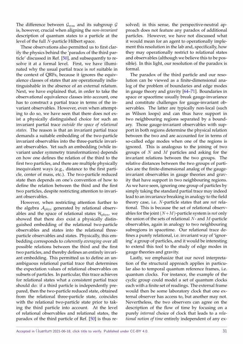
The difference between Gsym and its subgroup Gis, however, crucial when aligning the non-invariantdescription of quantum states to a particle at thelevel of the full N -particle Hilbert space.

These observations also permitted us to first clar-ify the physics behind the ’paradox of the third par-ticle’ discussed in Ref. [50], and subsequently to re-solve it at a formal level. First, we have illumi-nated why the usual partial trace is not suitable inthe context of QRFs, because it ignores the equiv-alence classes of states that are operationally indis-tinguishable in the absence of an external relatum.Next, we have explained that, in order to take theobservational equivalence classes into account, onehas to construct a partial trace in terms of the in-variant observables. However, even when attempt-ing to do so, we have seen that there does not ex-ist a physically distinguished choice for such aninvariant partial trace outside the space of relationalstates. The reason is that an invariant partial tracedemands a suitable embedding of the two-particleinvariant observables into the three-particle invari-ant observables. Yet such an embedding (while in-variant under symmetry transformations) dependson how one defines the relation of the third to thefirst two particles, and there are multiple physicallyinequivalent ways (e.g., distance to the first parti-cle, center of mass, etc.). The two-particle reducedstate then depends on one’s convention of how todefine the relation between the third and the firsttwo particles, despite restricting attention to invari-ant observables.

However, when restricting attention further tothe algebra Aphys generated by relational observ-ables and the space of relational states Hphys, weshowed that there does exist a physically distin-guished embedding of the relational two-particleobservables and states into the relational three-particle observables and states. Physically, this em-bedding corresponds to coherently averaging over allpossible relations between the third and the firsttwo particles, and thereby defines an entirely invari-ant embedding. This permitted us to define an un-ambiguous relational partial trace that determinesthe expectation values of relational observables onsubsets of particles. In particular, this trace achievesfor relational states what a consistent partial traceshould do: if a third particle is independently pre-pared, then the two-particle reduced state, obtainedfrom the relational three-particle state, coincideswith the relational two-particle state prior to tak-ing the third particle into account. At the levelof relational observables and relational states, theparadox of the third particle of Ref. [50] is thus re-

solved; in this sense, the perspective-neutral ap-proach does not feature any paradox of additionalparticles. However, we have not discussed whatit would mean for an agent to operationally imple-ment this resolution in the lab and, specifically, howthey may operationally restrict to relational statesand observables (although we believe this to be pos-sible). In this light, our resolution of the paradox isformal.

The paradox of the third particle and our reso-lution can be viewed as a finite-dimensional ana-log of the problem of boundaries and edge modesin gauge theory and gravity [64–71]. Boundaries inspace or spacetime usually break gauge-invarianceand constitute challenges for gauge-invariant ob-servables. The latter are typically non-local (suchas Wilson loops) and can thus have support intwo neighbouring regions separated by a bound-ary. Those gauge-invariant observables with sup-port in both regions determine the physical relationbetween the two and are accounted for in terms ofso-called edge modes when one of the regions isignored. This is analogous to the joining of twogroups of N and M particles and asking for theinvariant relations between the two groups. Therelative distances between the two groups of parti-cles are the finite-dimensional analog of the gauge-invariant observables in gauge theories and grav-ity that have support in two neighbouring regions.As we have seen, ignoring one group of particles bysimply taking the standard partial trace may indeedlead to an invariance breaking in analogy to the fieldtheory case, i.e. N -particle states that are not rela-tional. This is because the set of relational observ-ables for the joint (N+M)-particle system is not onlythe union of the sets of relational N - and M -particleobservables, again in analogy to two neighbouringsubregions in spacetime. Our relational trace de-fines a purely relational, i.e. invariant way of ‘ignor-ing’ a group of particles, and it would be interestingto extend this tool to the study of edge modes ingauge theories and gravity.

Lastly, we emphasize that our novel interpreta-tion of the structural approach applies in particu-lar also to temporal quantum reference frames, i.e.quantum clocks. For instance, the example of thecyclic group could model a set of quantum clockseach with a finite set of readings. The external framewould then be some laboratory clock that one ex-ternal observer has access to, but another may not.Nevertheless, the two observers can agree on thedescription of the flow of time by focusing on apurely internal choice of clock that leads to a rela-tional notion of time entirely independent of any ex-


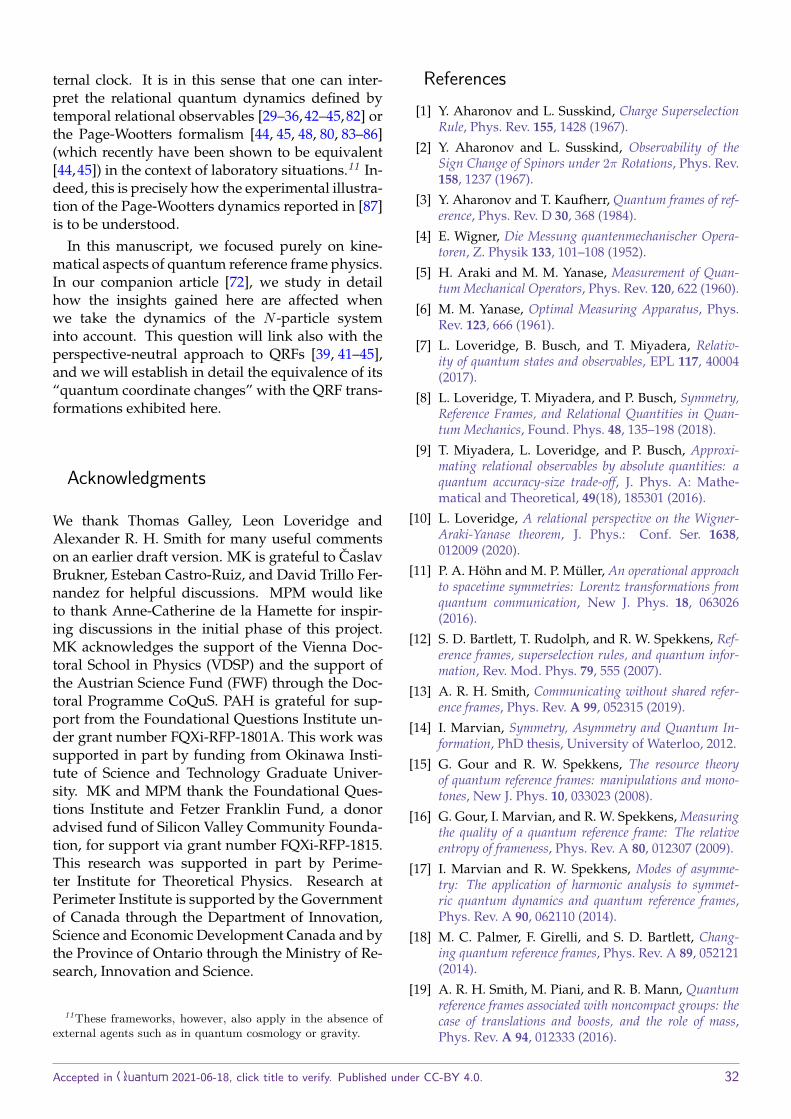
ternal clock. It is in this sense that one can inter-pret the relational quantum dynamics defined bytemporal relational observables [29–36,42–45,82] orthe Page-Wootters formalism [44, 45, 48, 80, 83–86](which recently have been shown to be equivalent[44,45]) in the context of laboratory situations.11 In-deed, this is precisely how the experimental illustra-tion of the Page-Wootters dynamics reported in [87]is to be understood.

In this manuscript, we focused purely on kine-matical aspects of quantum reference frame physics.In our companion article [72], we study in detailhow the insights gained here are affected whenwe take the dynamics of the N -particle systeminto account. This question will link also with theperspective-neutral approach to QRFs [39, 41–45],and we will establish in detail the equivalence of its“quantum coordinate changes” with the QRF trans-formations exhibited here.

Acknowledgments

We thank Thomas Galley, Leon Loveridge andAlexander R. H. Smith for many useful commentson an earlier draft version. MK is grateful to CaslavBrukner, Esteban Castro-Ruiz, and David Trillo Fer-nandez for helpful discussions. MPM would liketo thank Anne-Catherine de la Hamette for inspir-ing discussions in the initial phase of this project.MK acknowledges the support of the Vienna Doc-toral School in Physics (VDSP) and the support ofthe Austrian Science Fund (FWF) through the Doc-toral Programme CoQuS. PAH is grateful for sup-port from the Foundational Questions Institute un-der grant number FQXi-RFP-1801A. This work wassupported in part by funding from Okinawa Insti-tute of Science and Technology Graduate Univer-sity. MK and MPM thank the Foundational Ques-tions Institute and Fetzer Franklin Fund, a donoradvised fund of Silicon Valley Community Founda-tion, for support via grant number FQXi-RFP-1815.This research was supported in part by Perime-ter Institute for Theoretical Physics. Research atPerimeter Institute is supported by the Governmentof Canada through the Department of Innovation,Science and Economic Development Canada and bythe Province of Ontario through the Ministry of Re-search, Innovation and Science.

11These frameworks, however, also apply in the absence ofexternal agents such as in quantum cosmology or gravity.

References[1] Y. Aharonov and L. Susskind, Charge Superselection

Rule, Phys. Rev. 155, 1428 (1967).

[2] Y. Aharonov and L. Susskind, Observability of theSign Change of Spinors under 2π Rotations, Phys. Rev.158, 1237 (1967).

[3] Y. Aharonov and T. Kaufherr, Quantum frames of ref-erence, Phys. Rev. D 30, 368 (1984).

[4] E. Wigner, Die Messung quantenmechanischer Opera-toren, Z. Physik 133, 101–108 (1952).

[5] H. Araki and M. M. Yanase, Measurement of Quan-tum Mechanical Operators, Phys. Rev. 120, 622 (1960).

[6] M. M. Yanase, Optimal Measuring Apparatus, Phys.Rev. 123, 666 (1961).

[7] L. Loveridge, B. Busch, and T. Miyadera, Relativ-ity of quantum states and observables, EPL 117, 40004(2017).

[8] L. Loveridge, T. Miyadera, and P. Busch, Symmetry,Reference Frames, and Relational Quantities in Quan-tum Mechanics, Found. Phys. 48, 135–198 (2018).

[9] T. Miyadera, L. Loveridge, and P. Busch, Approxi-mating relational observables by absolute quantities: aquantum accuracy-size trade-off, J. Phys. A: Mathe-matical and Theoretical, 49(18), 185301 (2016).

[10] L. Loveridge, A relational perspective on the Wigner-Araki-Yanase theorem, J. Phys.: Conf. Ser. 1638,012009 (2020).

[11] P. A. Hohn and M. P. Muller, An operational approachto spacetime symmetries: Lorentz transformations fromquantum communication, New J. Phys. 18, 063026(2016).

[12] S. D. Bartlett, T. Rudolph, and R. W. Spekkens, Ref-erence frames, superselection rules, and quantum infor-mation, Rev. Mod. Phys. 79, 555 (2007).

[13] A. R. H. Smith, Communicating without shared refer-ence frames, Phys. Rev. A 99, 052315 (2019).

[14] I. Marvian, Symmetry, Asymmetry and Quantum In-formation, PhD thesis, University of Waterloo, 2012.

[15] G. Gour and R. W. Spekkens, The resource theoryof quantum reference frames: manipulations and mono-tones, New J. Phys. 10, 033023 (2008).

[16] G. Gour, I. Marvian, and R. W. Spekkens, Measuringthe quality of a quantum reference frame: The relativeentropy of frameness, Phys. Rev. A 80, 012307 (2009).

[17] I. Marvian and R. W. Spekkens, Modes of asymme-try: The application of harmonic analysis to symmet-ric quantum dynamics and quantum reference frames,Phys. Rev. A 90, 062110 (2014).

[18] M. C. Palmer, F. Girelli, and S. D. Bartlett, Chang-ing quantum reference frames, Phys. Rev. A 89, 052121(2014).

[19] A. R. H. Smith, M. Piani, and R. B. Mann, Quantumreference frames associated with noncompact groups: thecase of translations and boosts, and the role of mass,Phys. Rev. A 94, 012333 (2016).


https://doi.org/10.1103/PhysRev.155.1428





https://doi.org/10.1103/PhysRevD.30.368


https://doi.org/10.1007/BF01948686

https://doi.org/10.1007/BF01948686





https://doi.org/10.1209/0295-5075/117/40004

https://doi.org/10.1209/0295-5075/117/40004

https://doi.org/10.1209/0295-5075/117/40004

https://doi.org/10.1007/s10701-018-0138-3

https://doi.org/10.1007/s10701-018-0138-3

https://doi.org/10.1007/s10701-018-0138-3

https://doi.org/10.1088/1751-8113/49/18/185301

https://doi.org/10.1088/1751-8113/49/18/185301

https://doi.org/10.1088/1751-8113/49/18/185301

https://doi.org/10.1088/1751-8113/49/18/185301

https://doi.org/10.1088/1742-6596/1638/1/012009

https://doi.org/10.1088/1742-6596/1638/1/012009

https://doi.org/10.1088/1742-6596/1638/1/012009

https://doi.org/10.1088/1367-2630/18/6/063026

https://doi.org/10.1088/1367-2630/18/6/063026

https://doi.org/10.1088/1367-2630/18/6/063026

https://doi.org/10.1088/1367-2630/18/6/063026

https://doi.org/10.1103/RevModPhys.79.555



https://doi.org/10.1103/PhysRevA.99.052315


https://uwspace.uwaterloo.ca/handle/10012/7088

https://uwspace.uwaterloo.ca/handle/10012/7088

https://doi.org/10.1088/1367-2630/10/3/033023

https://doi.org/10.1088/1367-2630/10/3/033023

https://doi.org/10.1088/1367-2630/10/3/033023















[20] J. Aberg, Catalytic Coherence, Phys. Rev. Lett. 113,150402 (2014).

[21] M. Lostaglio, D. Jennings, and T. Rudolph, Descrip-tion of quantum coherence in thermodynamic processesrequires constraints beyond free energy, Nat. Commun.6, 6383 (2015).

[22] M. Lostaglio, K. Korzekwa, D. Jennings, and T.Rudolph, Quantum Coherence, Time-Translation Sym-metry, and Thermodynamics, Phys. Rev. X 5, 021001(2015).

[23] M. Lostaglio and M. P. Muller, Coherence and Asym-metry Cannot be Broadcast, Phys. Rev. Lett. 123,020403 (2019).

[24] I. Marvian and R. W. Spekkens, No-Broadcasting The-orem for Quantum Asymmetry and Coherence and aTrade-off Relation for Approximate Broadcasting, Phys.Rev. Lett. 123, 020404 (2019).

[25] P. Erker, M. T. Mitchison, R. Silva, M. P. Woods,N. Brunner, and M. Huber, Autonomous QuantumClocks: Does Thermodynamics Limit Our Ability toMeasure Time?, Phys. Rev. X 7, 031022 (2017).

[26] P. Cwiklinski, M. Studzinski, M. Horodecki, and J.Oppenheim, Limitations on the Evolution of QuantumCoherences: Towards Fully Quantum Second Laws ofThermodynamics, Phys. Rev. Lett. 115, 210403 (2015).

[27] M. P. Woods, R. Silva, and J. Oppenheim, Au-tonomous Quantum Machines and Finite-Sized Clocks,Ann. Henri Poincare 20, 125 (2019).

[28] M. P. Woods and M. Horodecki, The resource theo-retic paradigm of quantum thermodynamics with con-trol, arXiv:1912.05562 [quant-ph].

[29] C. Rovelli, Quantum gravity, Cambridge UniversityPress, 2004.

[30] T. Thiemann, Modern Canonical Quantum GeneralRelativity, Cambridge University Press, 2007.

[31] J. Tambornino, Relational Observables in Gravity: aReview, SIGMA 8, 017 (2012).

[32] C. Rovelli, What is observable in classical and quantumgravity?, Class. Quant. Grav. 8, 297 (1991).

[33] C. Rovelli, Quantum reference systems, Class. Quant.Grav. 8, 317 (1991).

[34] C. Rovelli, Time in quantum gravity: An hypothesis,Phys. Rev. D 43, 442-456 (1991).

[35] B. Dittrich, Partial and complete observables for Hamil-tonian constrained systems, Gen. Rel. Grav. 39, 1891(2007).

[36] B. Dittrich, Partial and complete observables for canon-ical general relativity, Class. Quant. Grav. 23, 6155(2006).

[37] L. Chataignier, Construction of quantum Dirac observ-ables and the emergence of WKB time, Phys. Rev. D 101,086001 (2020).

[38] F. Giacomini, E. Castro-Ruiz, and C. Brukner, Quan-tum mechanics and the covariance of physical laws inquantum reference frames, Nat. Commun. 10, 494(2019).

[39] A. Vanrietvelde, P. A. Hohn, F. Giacomini, and E.Castro-Ruiz, A change of perspective: switching quan-tum reference frames via a perspective-neutral frame-work, Quantum 4, 225 (2020).

[40] A. de la Hamette and T. Galley, Quantum referenceframes for general symmetry groups, Quantum 4, 367(2020).

[41] A. Vanrietvelde, P. A. Hohn, and F. Giacomini,Switching quantum reference frames in the N-body prob-lem and the absence of global relational perspectives,arXiv:1809.05093 [quant-ph].

[42] P. A. Hohn and A. Vanrietvelde, How to switch be-tween relational quantum clocks, New J. Phys. 22,123048 (2020).

[43] P. A. Hohn, Switching Internal Times and a New Per-spective on the ‘Wave Function of the Universe’, Uni-verse 5, 116 (2019).

[44] P. A. Hohn, A. R. H. Smith, and M. P. E. Lock, TheTrinity of Relational Quantum Dynamics, Phys. Rev. D(in press), arXiv:1912.00033 [quant-ph].

[45] P. A. Hohn, A. R. H. Smith, and M. P. E. Lock, Equiv-alence of approaches to relational quantum dynamics inrelativistic settings, Front. Phys. 9, 587083 (2021).

[46] F. Giacomini, E. Castro-Ruiz, and C. Brukner, Rel-ativistic Quantum Reference Frames: The OperationalMeaning of Spin, Phys. Rev. Lett. 123, 090404 (2019).

[47] L. F. Streiter, F. Giacomini, and C. Brukner, A Rel-ativistic Bell Test within Quantum Reference Frames,Phys. Rev. Lett. 126, 230403 (2021).

[48] E. Castro-Ruiz, F. Giacomini, A. Belenchia, and C.Brukner, Quantum clocks and the temporal localisabilityof events in the presence of gravitating quantum systems,Nat. Commun. 11, 2672 (2020).

[49] J. M. Yang, Switching Quantum Reference Frames forQuantum Measurement, Quantum 4, 283 (2020).

[50] R. M. Angelo, N. Brunner, S. Popescu, A. J. Short,and P. Skrzypczyk, Physics within a quantum referenceframe, J. Phys. A: Math. Theor. 44, 145304 (2011).

[51] T. P. Le, P. Mironowicz, and P. Horodecki, Blurredquantum Darwinism across quantum reference frames,Phys. Rev. A 102, 062420 (2020).

[52] J. Tuziemski, Decoherence and information encoding inquantum reference frames, arXiv:2006.07298 [quant-ph].

[53] M. F. Savi, and R. M. Angelo, Quantum Resources Co-variance, Phys. Rev. A 103, 022220 (2021).

[54] P. A. Guerin and C. Brukner, Observer-dependent lo-cality of quantum events, New J. Phys. 20, 103031(2018).

[55] L. Hardy, Implementation of the Quantum EquivalencePrinciple, arXiv:1903.01289 [quant-ph].

[56] S. Gielen and L. Menendez-Pidal, Singularity reso-lution depends on the clock, Class. Quant. Grav. 37,205018 (2020).


https://doi.org/10.1103/PhysRevLett.113.150402


https://doi.org/https://doi.org/10.1038/ncomms7383




https://doi.org/10.1103/PhysRevX.5.021001
















https://doi.org/10.1007/s00023-018-0736-9

https://doi.org/10.1007/s00023-018-0736-9

https://doi.org/10.1007/s00023-018-0736-9

https://arxiv.org/abs/1912.05562



http://arxiv.org/abs/1912.05562

https://doi.org/10.1017/CBO9780511755804

https://doi.org/10.1017/CBO9780511755804

https://doi.org/10.1017/CBO9780511755682

https://doi.org/10.1017/CBO9780511755682

https://doi.org/10.3842/SIGMA.2012.017

https://doi.org/10.3842/SIGMA.2012.017

https://doi.org/10.1088/0264-9381/8/2/011

https://doi.org/10.1088/0264-9381/8/2/011

https://doi.org/10.1088/0264-9381/8/2/012

https://doi.org/10.1088/0264-9381/8/2/012



https://doi.org/10.1007/s10714-007-0495-2

https://doi.org/10.1007/s10714-007-0495-2

https://doi.org/10.1007/s10714-007-0495-2

https://doi.org/10.1088/0264-9381/23/22/006

https://doi.org/10.1088/0264-9381/23/22/006

https://doi.org/10.1088/0264-9381/23/22/006




https://doi.org/10.1038/s41467-018-08155-0

https://doi.org/10.1038/s41467-018-08155-0

https://doi.org/10.1038/s41467-018-08155-0

https://doi.org/10.1038/s41467-018-08155-0

https://doi.org/10.22331/q-2020-01-27-225

https://doi.org/10.22331/q-2020-01-27-225

https://doi.org/10.22331/q-2020-01-27-225

https://doi.org/10.22331/q-2020-11-30-367

https://doi.org/10.22331/q-2020-11-30-367

https://doi.org/10.22331/q-2020-11-30-367





https://doi.org/10.1088/1367-2630/abd1ac



https://doi.org/10.3390/universe5050116







https://doi.org/10.3389/fphy.2021.587083









https://doi.org/10.1038/s41467-020-16013-1

https://doi.org/10.1038/s41467-020-16013-1

https://doi.org/10.1038/s41467-020-16013-1

https://doi.org/10.22331/q-2020-06-18-283

https://doi.org/10.22331/q-2020-06-18-283

https://doi.org/10.1088/1751-8113/44/14/145304

https://doi.org/10.1088/1751-8113/44/14/145304










https://doi.org/10.1088/1367-2630/aae742

https://doi.org/10.1088/1367-2630/aae742

https://doi.org/10.1088/1367-2630/aae742




https://doi.org/10.1088/1361-6382/abb14f



[57] K. Giesel, L. Herold, B. F. Li, and P. Singh,Mukhanov-Sasaki equation in a manifestly gauge-invariant linearized cosmological perturbation theorywith dust reference fields, Phys. Rev. D 102, 023524(2020).

[58] K. Giesel, B. F. Li, and P. Singh, Towards a re-duced phase space quantization in loop quantum cosmol-ogy with an inflationary potential, Phys. Rev. D 102,126024 (2020).

[59] P. A. Dirac, Lectures on Quantum Mechanics, YeshivaUniversity Press, 1964.

[60] M. Henneaux and C. Teitelboim, Quantization ofGauge Systems, Princeton University Press, 1992.

[61] D. Giulini and D. Marolf, A Uniqueness theorem forconstraint quantization, Class. Quant. Grav. 16, 2489(1999).

[62] D. Marolf, Group averaging and refined algebraic quan-tization: Where are we now?, arXiv:gr-qc/0011112 [gr-qc].

[63] C. Rovelli, Why Gauge?, Found. Phys. 44, 91–104(2014).

[64] W. Donnelly and A. C. Wall, Entanglement Entropyof Electromagnetic Edge Modes, Phys. Rev. Lett. 114,111603 (2015).

[65] W. Donnelly and L. Freidel, Local subsystems in gaugetheory and gravity, JHEP 09, 102 (2016).

[66] M. Geiller and P. Jai-akson, Extended actions, dynam-ics of edge modes, and entanglement entropy, JHEP 20,134 (2020).

[67] L. Freidel, M. Geiller and D. Pranzetti, Edge modesof gravity. Part I. Corner potentials and charges, JHEP2020, 26 (2020).

[68] H. Gomes and A. Riello, Unified geometric frameworkfor boundary charges and particle dressings, Phys. Rev.D 98, 025013 (2018).

[69] A. Riello, Symplectic reduction of Yang-Mills theorywith boundaries: from superselection sectors to edgemodes, and back, SciPost Phys. 10, 125 (2021).

[70] W. Wieland, New boundary variables for classical andquantum gravity on a null surface, Class. Quant. Grav.34, no.21, 215008 (2017).

[71] W. Wieland, Fock representation of gravitational bound-ary modes and the discreteness of the area spectrum, An-nales Henri Poincare 18, no.11, 3695 (2017).

[72] P. A. Hohn, M. Krumm, and M. P. Muller, Inter-nal quantum reference frames for finite Abelian groups,arXiv:2107.07545 [quant-ph].

[73] B. Simon, Representations of Finite and CompactGroups, American Mathematical Society, 1996.

[74] K. R. Davidson, C∗-Algebras by Example, AmericanMathematical Society, 1996.

[75] A. Savage, Modern Group Theory, lecture notes,University of Ottawa, 2017. Available athttps://alistairsavage.ca/mat5145/notes/MAT5145-Modern_group_theory.pdf

[76] P. A. Hohn, Reflections on the information paradigm inquantum and gravitational physics, J. Phys. Conf. Ser.880, 012014 (2017).

[77] M. A. Nielsen and I. L. Chuang, Quantum Compu-tation and Quantum Information, Cambridge Univer-sity Press, New York, 2010.

[78] M. Tinkham, Group Theory and Quantum Mechanics,Dover Publications, 1992.

[79] S. Khandelwal, M. P. E. Lock, and M. P. Woods, Uni-versal quantum modifications to general relativistic timedilation in delocalised clocks, Quantum 4, 309 (2020).

[80] A. R. H. Smith and M. Ahmadi, Quantum clocks ob-serve classical and quantum time dilation, Nat. Com-mun. 11, 5360 (2020).

[81] P. T. Grochowski, A. R. H. Smith, A. Dragan, and K.Debski, Quantum time dilation in atomic spectra, Phys.Rev. Research 3, 023053 (2021).

[82] R. Gambini and J. Pullin, The Montevideo Interpreta-tion: How the inclusion of a Quantum Gravitational No-tion of Time Solves the Measurement Problem, Universe6, 236 (2020).

[83] D. N. Page, and W. K. Wootters, Evolution with-out evolution: Dynamics described by stationary observ-ables, Phys. Rev. D 27, 2885 (1983).

[84] W. K. Wootters, “Time” replaced by quantum correla-tions, Int. J. Theor. Phys. 23, 701 (1984).

[85] V. Giovannetti, S. Lloyd, and L. Maccone, Quantumtime, Phys. Rev. D 92, 045033 (2015).

[86] A. R. H. Smith and M. Ahmadi, Quantizing time: in-teracting clocks and systems, Quantum 3, 160 (2019).

[87] E. Moreva, G. Brida, M. Gramegna, V. Giovannetti,L. Maccone, and M. Genovese, Time from quantumentanglement: An experimental illustration, Phys. Rev.A 89, 052122 (2014).










https://doi.org/10.1515/9780691213866

https://doi.org/10.1515/9780691213866

https://doi.org/10.1088/0264-9381/16/7/322

https://doi.org/10.1088/0264-9381/16/7/322

https://doi.org/10.1088/0264-9381/16/7/322

https://arxiv.org/abs/gr-qc/0011112


http://arxiv.org/abs/gr-qc/0011112


https://doi.org/10.1007/s10701-013-9768-7

https://doi.org/10.1007/s10701-013-9768-7




https://doi.org/10.1007/JHEP09(2016)102











https://doi.org/10.21468/SciPostPhys.10.6.125



https://doi.org/10.1088/1361-6382/aa8d06

https://doi.org/10.1088/1361-6382/aa8d06

https://doi.org/10.1088/1361-6382/aa8d06

https://doi.org/10.1007/s00023-017-0598-6

https://doi.org/10.1007/s00023-017-0598-6

https://doi.org/10.1007/s00023-017-0598-6





https://alistairsavage.ca/mat5145/notes/MAT5145-Modern_group_theory.pdf

https://alistairsavage.ca/mat5145/notes/MAT5145-Modern_group_theory.pdf

https://doi.org/10.1088/1742-6596/880/1/012014

https://doi.org/10.1088/1742-6596/880/1/012014

https://doi.org/10.1088/1742-6596/880/1/012014

https://doi.org/10.1017/CBO9780511976667

https://doi.org/10.1017/CBO9780511976667

https://doi.org/10.1017/CBO9780511976667

https://doi.org/10.22331/q-2020-08-14-309

https://doi.org/10.22331/q-2020-08-14-309

https://doi.org/10.22331/q-2020-08-14-309

https://doi.org/10.1038/s41467-020-18264-4

https://doi.org/10.1038/s41467-020-18264-4

https://doi.org/10.1038/s41467-020-18264-4

https://doi.org/10.1103/PhysRevResearch.3.023053

https://doi.org/10.1103/PhysRevResearch.3.023053








https://doi.org/10.1007/BF02214098

https://doi.org/10.1007/BF02214098



https://doi.org/10.22331/q-2019-07-08-160

https://doi.org/10.22331/q-2019-07-08-160




Quantum reference frame transformations as symmetries and ...

Documents

Transcript of Quantum reference frame transformations as symmetries and ...