Hadron Physics in Tests of Fundamental Symmetries
225
University of Massachusetts Amherst University of Massachusetts Amherst ScholarWorks@UMass Amherst ScholarWorks@UMass Amherst Doctoral Dissertations Dissertations and Theses July 2016 Hadron Physics in Tests of Fundamental Symmetries Hadron Physics in Tests of Fundamental Symmetries Chien Yeah Seng University of Massachusetts Amherst Follow this and additional works at: https://scholarworks.umass.edu/dissertations_2 Part of the Elementary Particles and Fields and String Theory Commons, Nuclear Commons, and the Quantum Physics Commons Recommended Citation Recommended Citation Seng, Chien Yeah, "Hadron Physics in Tests of Fundamental Symmetries" (2016). Doctoral Dissertations. 688. https://doi.org/10.7275/8416905.0 https://scholarworks.umass.edu/dissertations_2/688 This Open Access Dissertation is brought to you for free and open access by the Dissertations and Theses at ScholarWorks@UMass Amherst. It has been accepted for inclusion in Doctoral Dissertations by an authorized administrator of ScholarWorks@UMass Amherst. For more information, please contact [email protected].
-
Upload
khangminh22 -
Category
Documents
-
view
0 -
download
0
Transcript of Hadron Physics in Tests of Fundamental Symmetries
University of Massachusetts Amherst University of Massachusetts Amherst
ScholarWorks@UMass Amherst ScholarWorks@UMass Amherst
Doctoral Dissertations Dissertations and Theses
July 2016
Hadron Physics in Tests of Fundamental Symmetries Hadron Physics in Tests of Fundamental Symmetries
Chien Yeah Seng University of Massachusetts Amherst
Follow this and additional works at: https://scholarworks.umass.edu/dissertations_2
Part of the Elementary Particles and Fields and String Theory Commons, Nuclear Commons, and the
Quantum Physics Commons
Recommended Citation Recommended Citation Seng, Chien Yeah, "Hadron Physics in Tests of Fundamental Symmetries" (2016). Doctoral Dissertations. 688. https://doi.org/10.7275/8416905.0 https://scholarworks.umass.edu/dissertations_2/688
This Open Access Dissertation is brought to you for free and open access by the Dissertations and Theses at ScholarWorks@UMass Amherst. It has been accepted for inclusion in Doctoral Dissertations by an authorized administrator of ScholarWorks@UMass Amherst. For more information, please contact [email protected].
HADRON PHYSICS IN TESTS OF FUNDAMENTAL
SYMMETRIES
A Dissertation Presented
by
CHIEN YEAH SENG
Submitted to the Graduate School of theUniversity of Massachusetts Amherst in partial fulfillment
of the requirements for the degree of
DOCTOR OF PHILOSOPHY
May 2016
Department of Physics
c© Copyright by Chien Yeah Seng 2016
All Rights Reserved
HADRON PHYSICS IN TESTS OF FUNDAMENTAL
SYMMETRIES
A Dissertation Presented
by
CHIEN YEAH SENG
Approved as to style and content by:
Michael J. Ramsey-Musolf, Chair
Barry Holstein, Member
Lorenzo Sorbo, Member
Hongkun Zhang, Member
Rory Miskimen, Department ChairDepartment of Physics
DEDICATION
To my family
ACKNOWLEDGMENTS
The completion of this thesis as well as my PhD study would be impossible without
the help from many people whom I wish to take this opportunity to express my deepest
gratitude to.
First of all I wish to thank Prof. Michael Ramsey-Musolf, my PhD advisor and
thesis committee chair. He is the person who raised my entire interest and guided
me into the area of QCD and hadron physics. He is also a great teacher who teaches
me how to live and work like a true researcher. Next, I would like to also express my
gratitude to all the other members in my thesis committee: Prof. Barry Holstein,
Prof. Lorenzo Sorbo and Prof. Hongkun Zhang. The whole procedure would be
impossible without their active participation. Also, I want to pay special thanks to
Carlo Dallapiccola and Jane Knapp, the graduate program director and manager.
They provided me countless helps during my PhD life in Amherst.
I am also extremely grateful to all the previous and current colleagues in my re-
search group, both in Wisconsin and in UMass. In particular, I wish to give very
special thanks to Hiren Patel, Mario Pitschmann and Huaike Guo as I have learned a
lot from them through formal and informal discussions. Of course, all my collabora-
tors in various projects will never be forgotten as well. I wish to express my gratitude
to Jordy de Vries, Emanuele Mereghetti and Craig Roberts. They are no mere col-
laborators of mine but are also extremely helpful in shaping my research career in
general.
Next, I am indebted to all the professors whom I learned physics from, in particular
to Prof. Daniel Chung from University of Wisconsin-Madison for everything he taught
v
me about Quantum Field Theory. His lectures notes are so clear and detailed that I
am always benefited from them during my research.
Last but not least, I want to thank my dad Ah Loke Seng, my mom Suk Hen Kok,
my elder brother Chien Wei Seng and my girlfriend Fang Ye. I simply wouldn’t be
myself without them playing their roles in my life.
vi
ABSTRACT
HADRON PHYSICS IN TESTS OF FUNDAMENTAL
SYMMETRIES
MAY 2016
CHIEN YEAH SENG
B.Sc., TSINGHUA UNIVERSITY
M.P.H., HONG KONG UNIVERSITY OF SCIENCE AND TECHNOLOGY
Ph.D., UNIVERSITY OF MASSACHUSETTS AMHERST
Directed by: Professor Michael J. Ramsey-Musolf
Low energy precision tests of fundamental symmetries provide excellent probes
for the Beyond Standard Model Physics. Theoretical interpretations of these exper-
iments often involve the application of non-perturbative Quantum Chromodynamics
in the study of hadronic matrix elements that may either serve as signals of new
physics or Standard Model backgrounds. In this work I present a series of studies on
different hadronic matrix elements using various low-energy effective approaches to
Quantum Chromodynamics, and discuss the impact of these studies on our knowledge
of Standard Model and Beyond Standard Model physics.
vii
TABLE OF CONTENTS
Page
ACKNOWLEDGMENTS . . . . . . . . . . . . . . . . . . . . . . . . . . . . . . . . . . . . . . . . . . . . v
ABSTRACT . . . . . . . . . . . . . . . . . . . . . . . . . . . . . . . . . . . . . . . . . . . . . . . . . . . . . . . . vii
LIST OF TABLES . . . . . . . . . . . . . . . . . . . . . . . . . . . . . . . . . . . . . . . . . . . . . . . . . . xii
LIST OF FIGURES . . . . . . . . . . . . . . . . . . . . . . . . . . . . . . . . . . . . . . . . . . . . . . . . .xiv
CHAPTER
INTRODUCTION . . . . . . . . . . . . . . . . . . . . . . . . . . . . . . . . . . . . . . . . . . . . . . . . . . . 1
1. ELECTRIC DIPOLE MOMENT OF THE ρ-MESON . . . . . . . . . . . . 12
1.1 Introduction . . . . . . . . . . . . . . . . . . . . . . . . . . . . . . . . . . . . . . . . . . . . . . . . . . . . 121.2 ρ-meson as a Bound State . . . . . . . . . . . . . . . . . . . . . . . . . . . . . . . . . . . . . . . . 15
1.2.1 ρ-γ Vertex . . . . . . . . . . . . . . . . . . . . . . . . . . . . . . . . . . . . . . . . . . . . . . . 151.2.2 Contact Interaction . . . . . . . . . . . . . . . . . . . . . . . . . . . . . . . . . . . . . . . . 16
1.3 ρ-meson Form Factors . . . . . . . . . . . . . . . . . . . . . . . . . . . . . . . . . . . . . . . . . . . . 201.4 ρ-meson EDM: Formulae . . . . . . . . . . . . . . . . . . . . . . . . . . . . . . . . . . . . . . . . . 24
1.4.1 Four-fermion interaction . . . . . . . . . . . . . . . . . . . . . . . . . . . . . . . . . . . 25
1.4.1.1 L6 – quark-photon vertex . . . . . . . . . . . . . . . . . . . . . . . . . . 261.4.1.2 L6 – Bethe-Salpeter amplitude . . . . . . . . . . . . . . . . . . . . . . 271.4.1.3 L6 – quark propagator . . . . . . . . . . . . . . . . . . . . . . . . . . . . . 28
1.4.2 Quark chromo-EDM . . . . . . . . . . . . . . . . . . . . . . . . . . . . . . . . . . . . . . . 28
1.4.2.1 LCEDM – quark-photon vertex . . . . . . . . . . . . . . . . . . . . . . 291.4.2.2 LCEDM – Bethe-Salpeter amplitude . . . . . . . . . . . . . . . . . . 301.4.2.3 LCEDM – quark propagator . . . . . . . . . . . . . . . . . . . . . . . . . 31
1.4.3 θ-term . . . . . . . . . . . . . . . . . . . . . . . . . . . . . . . . . . . . . . . . . . . . . . . . . . . 31
viii
1.4.3.1 Dressed-quark anomalous chromomagneticmoment . . . . . . . . . . . . . . . . . . . . . . . . . . . . . . . . . . . . . . . 32
1.5 ρ-meson EDM: Results . . . . . . . . . . . . . . . . . . . . . . . . . . . . . . . . . . . . . . . . . . . 34
1.5.1 Analysis without Peccei-Quinn symmetry . . . . . . . . . . . . . . . . . . . . . 341.5.2 Peccei Quinn Symmetry . . . . . . . . . . . . . . . . . . . . . . . . . . . . . . . . . . . . 37
1.6 Epilogue . . . . . . . . . . . . . . . . . . . . . . . . . . . . . . . . . . . . . . . . . . . . . . . . . . . . . . . 39
2. SCALAR AND TENSOR CHARGES OF THE NUCLEON . . . . . . 43
2.1 Introduction . . . . . . . . . . . . . . . . . . . . . . . . . . . . . . . . . . . . . . . . . . . . . . . . . . . . 432.2 Nucleon Faddeev Amplitude and Relevant Interaction Currents . . . . . . . . 472.3 Sigma-Term . . . . . . . . . . . . . . . . . . . . . . . . . . . . . . . . . . . . . . . . . . . . . . . . . . . . 482.4 Tensor Charge . . . . . . . . . . . . . . . . . . . . . . . . . . . . . . . . . . . . . . . . . . . . . . . . . . 512.5 Electric Dipole Moments . . . . . . . . . . . . . . . . . . . . . . . . . . . . . . . . . . . . . . . . . 572.6 Conclusion . . . . . . . . . . . . . . . . . . . . . . . . . . . . . . . . . . . . . . . . . . . . . . . . . . . . . 59
3. AN INTRODUCTION TO THE CHIRAL PERTURBATION
THEORY . . . . . . . . . . . . . . . . . . . . . . . . . . . . . . . . . . . . . . . . . . . . . . . . . . . . . . 61
3.1 The motivation . . . . . . . . . . . . . . . . . . . . . . . . . . . . . . . . . . . . . . . . . . . . . . . . . . 613.2 Chiral symmetry and spontaneous symmetry breaking . . . . . . . . . . . . . . . . 62
3.2.1 Chiral transformation . . . . . . . . . . . . . . . . . . . . . . . . . . . . . . . . . . . . . . 623.2.2 Spontaneous symmetry breaking . . . . . . . . . . . . . . . . . . . . . . . . . . . . 64
3.3 Non-linear realization of NG bosons . . . . . . . . . . . . . . . . . . . . . . . . . . . . . . . . 65
3.3.1 Basic idea . . . . . . . . . . . . . . . . . . . . . . . . . . . . . . . . . . . . . . . . . . . . . . . . 653.3.2 Example of non-linear realization: SU(2)L × SU(2)R . . . . . . . . . . . 66
3.4 ChPT for NG bosons . . . . . . . . . . . . . . . . . . . . . . . . . . . . . . . . . . . . . . . . . . . . 67
3.4.1 O(p2): Chiral invariant terms . . . . . . . . . . . . . . . . . . . . . . . . . . . . . . . 683.4.2 Spurion and chiral symmetry breaking terms at O(p2) . . . . . . . . . . 693.4.3 Brief discussion of O(p4) Lagrangian . . . . . . . . . . . . . . . . . . . . . . . . . 70
3.5 Baryons in ChPT . . . . . . . . . . . . . . . . . . . . . . . . . . . . . . . . . . . . . . . . . . . . . . . . 71
3.5.1 Transformation rule of the nucleon field . . . . . . . . . . . . . . . . . . . . . . 713.5.2 Nucleon Lagrangian at O(p1) . . . . . . . . . . . . . . . . . . . . . . . . . . . . . . . 73
3.6 Heavy Baryon Chiral Perturbation Theory . . . . . . . . . . . . . . . . . . . . . . . . . . 74
3.6.1 The velocity superselection rule . . . . . . . . . . . . . . . . . . . . . . . . . . . . . 75
ix
3.6.2 Light and heavy components of the nucleon field . . . . . . . . . . . . . . 763.6.3 The heavy baryon expansion . . . . . . . . . . . . . . . . . . . . . . . . . . . . . . . . 773.6.4 Reduction of Dirac structures . . . . . . . . . . . . . . . . . . . . . . . . . . . . . . . 783.6.5 Leading order HBChPT Lagrangian . . . . . . . . . . . . . . . . . . . . . . . . . 80
4. NUCLEON ELECTRIC DIPOLE MOMENTS AND THE
ISOVECTOR PARITY- AND TIME-REVERSAL-ODD
PION-NUCLEON COUPLING . . . . . . . . . . . . . . . . . . . . . . . . . . . . . . . . 81
4.1 Introduction . . . . . . . . . . . . . . . . . . . . . . . . . . . . . . . . . . . . . . . . . . . . . . . . . . . . 814.2 HBChPT Calculation . . . . . . . . . . . . . . . . . . . . . . . . . . . . . . . . . . . . . . . . . . . . 854.3 Comparison with Earlier Work . . . . . . . . . . . . . . . . . . . . . . . . . . . . . . . . . . . . 944.4 Implications and Conclusions . . . . . . . . . . . . . . . . . . . . . . . . . . . . . . . . . . . . . . 96
5. REEXAMINATION OF THE STANDARD MODEL
NUCLEON ELECTRIC DIPOLE MOMENT . . . . . . . . . . . . . . . . . . 98
5.1 HBchPT: Strong and Electroweak Interactions . . . . . . . . . . . . . . . . . . . . . . 1025.2 Determination of the LECs . . . . . . . . . . . . . . . . . . . . . . . . . . . . . . . . . . . . . . 1075.3 One loop contribution . . . . . . . . . . . . . . . . . . . . . . . . . . . . . . . . . . . . . . . . . . . 1115.4 Pole Contribution . . . . . . . . . . . . . . . . . . . . . . . . . . . . . . . . . . . . . . . . . . . . . . 1165.5 Discussion and Summary . . . . . . . . . . . . . . . . . . . . . . . . . . . . . . . . . . . . . . . . 118
6. HIGHER-TWIST CORRECTION TO PVDIS AND ITS
RELATION TO THE PARTON ANGULAR
MOMENTUM . . . . . . . . . . . . . . . . . . . . . . . . . . . . . . . . . . . . . . . . . . . . . . . . 121
6.1 Introduction . . . . . . . . . . . . . . . . . . . . . . . . . . . . . . . . . . . . . . . . . . . . . . . . . . . 1216.2 Higher-twist in PVDIS: general formulation . . . . . . . . . . . . . . . . . . . . . . . . 1246.3 The light-cone amplitudes . . . . . . . . . . . . . . . . . . . . . . . . . . . . . . . . . . . . . . . 1276.4 Matrix elements between nucleon states . . . . . . . . . . . . . . . . . . . . . . . . . . . 1296.5 Numerical results and discussion . . . . . . . . . . . . . . . . . . . . . . . . . . . . . . . . . . 1356.6 Summary . . . . . . . . . . . . . . . . . . . . . . . . . . . . . . . . . . . . . . . . . . . . . . . . . . . . . . 139
7. CONCLUSION . . . . . . . . . . . . . . . . . . . . . . . . . . . . . . . . . . . . . . . . . . . . . . . . . 141
APPENDICES
A. CONTACT INTERACTION . . . . . . . . . . . . . . . . . . . . . . . . . . . . . . . . . . . . 145
B. FADDEEV EQUATION . . . . . . . . . . . . . . . . . . . . . . . . . . . . . . . . . . . . . . . . . 149
C. INTERACTION CURRENTS . . . . . . . . . . . . . . . . . . . . . . . . . . . . . . . . . . 156
D. ON-SHELL CONSIDERATIONS FOR THE TRANSITION
DIAGRAMS . . . . . . . . . . . . . . . . . . . . . . . . . . . . . . . . . . . . . . . . . . . . . . . . . . 177
E. MODEL SCALE . . . . . . . . . . . . . . . . . . . . . . . . . . . . . . . . . . . . . . . . . . . . . . . . 179
x
F. SCALE DEPENDENCE OF THE TENSOR CHARGE . . . . . . . . . . 181
G. EUCLIDEAN CONVENTIONS . . . . . . . . . . . . . . . . . . . . . . . . . . . . . . . . . 182
H. MATRIX ELEMENTS OF TWO AND FOUR-FERMION
OPERATORS . . . . . . . . . . . . . . . . . . . . . . . . . . . . . . . . . . . . . . . . . . . . . . . . 184
I. COMPLETE FORMULAE FOR VARIOUS QUARK
DISTRIBUTION FUNCTIONS IN TERMS OF PROTON
WAVEFUNCTION AMPLITUDES . . . . . . . . . . . . . . . . . . . . . . . . . . . 186
J. VANISHING ONE-LOOP DIAGRAMS IN THE
CALCULATIONS OF SM NUCLEON EDM . . . . . . . . . . . . . . . . . . 190
BIBLIOGRAPHY . . . . . . . . . . . . . . . . . . . . . . . . . . . . . . . . . . . . . . . . . . . . . . . . . 192
xi
LIST OF TABLES
Table Page
I.1 Examples of current upper bounds on EDM of particles . . . . . . . . . . . . . . . . 6
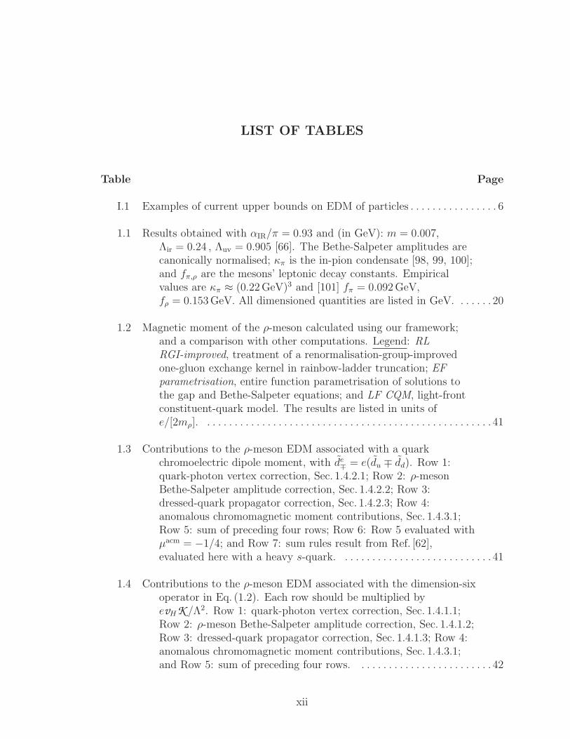
1.1 Results obtained with αIR/π = 0.93 and (in GeV): m = 0.007,Λir = 0.24 , Λuv = 0.905 [66]. The Bethe-Salpeter amplitudes arecanonically normalised; κπ is the in-pion condensate [98, 99, 100];and fπ,ρ are the mesons’ leptonic decay constants. Empiricalvalues are κπ ≈ (0.22 GeV)3 and [101] fπ = 0.092 GeV,fρ = 0.153 GeV. All dimensioned quantities are listed in GeV. . . . . . . 20
1.2 Magnetic moment of the ρ-meson calculated using our framework;and a comparison with other computations. Legend: RLRGI-improved, treatment of a renormalisation-group-improvedone-gluon exchange kernel in rainbow-ladder truncation; EFparametrisation, entire function parametrisation of solutions tothe gap and Bethe-Salpeter equations; and LF CQM, light-frontconstituent-quark model. The results are listed in units ofe/[2mρ]. . . . . . . . . . . . . . . . . . . . . . . . . . . . . . . . . . . . . . . . . . . . . . . . . . . . . 41
1.3 Contributions to the ρ-meson EDM associated with a quarkchromoelectric dipole moment, with de
∓ = e(du ∓ dd). Row 1:quark-photon vertex correction, Sec. 1.4.2.1; Row 2: ρ-mesonBethe-Salpeter amplitude correction, Sec. 1.4.2.2; Row 3:dressed-quark propagator correction, Sec. 1.4.2.3; Row 4:anomalous chromomagnetic moment contributions, Sec. 1.4.3.1;Row 5: sum of preceding four rows; Row 6: Row 5 evaluated withµacm = −1/4; and Row 7: sum rules result from Ref. [62],evaluated here with a heavy s-quark. . . . . . . . . . . . . . . . . . . . . . . . . . . . 41
1.4 Contributions to the ρ-meson EDM associated with the dimension-sixoperator in Eq. (1.2). Each row should be multiplied byevHK /Λ2. Row 1: quark-photon vertex correction, Sec. 1.4.1.1;Row 2: ρ-meson Bethe-Salpeter amplitude correction, Sec. 1.4.1.2;Row 3: dressed-quark propagator correction, Sec. 1.4.1.3; Row 4:anomalous chromomagnetic moment contributions, Sec. 1.4.3.1;and Row 5: sum of preceding four rows. . . . . . . . . . . . . . . . . . . . . . . . . 42
xii
5.1 Different contributions to the SM neutron and proton EDM in unitsof e cm, assuming the sign of LECs are those given in SectionIII. . . . . . . . . . . . . . . . . . . . . . . . . . . . . . . . . . . . . . . . . . . . . . . . . . . . . . . . . 118
6.1 The contributions from different lz-components to Q±p (xB). The
lz=0,+1 components contribute mostly to Q−p (“dominant”) and
less so to Q+p (“subdominant”), while the lz=-1 component
contributes only to Q+p . . . . . . . . . . . . . . . . . . . . . . . . . . . . . . . . . . . . . . . . 134
6.2 The dependence on different quark light-cone OAM components ofvarious distribution functions. . . . . . . . . . . . . . . . . . . . . . . . . . . . . . . . . . 139
C.1 Column 1: Summary of the results computed from all diagramsconsidered in connection with the proton’s charge. Column 2:Results scaled as described in Sec. C.1.7. . . . . . . . . . . . . . . . . . . . . . . . . 164
C.2 Summary of the results computed from all diagrams considered inconnection with the proton’s scalar charge. . . . . . . . . . . . . . . . . . . . . . . 169
C.3 Summary of results computed from all diagrams considered inconnection with the proton’s tensor charge. They represent valuesat the model scale, ζH ≈M , described in App. E. . . . . . . . . . . . . . . . 174
C.4 Summary of results computed from all diagrams considered inconnection with the proton’s tensor charge using input based onαIR/π = 0.74, quoted at the model scale, ζH ≈M , described inApp. E. . . . . . . . . . . . . . . . . . . . . . . . . . . . . . . . . . . . . . . . . . . . . . . . . . . . . 176
xiii
LIST OF FIGURES
Figure Page
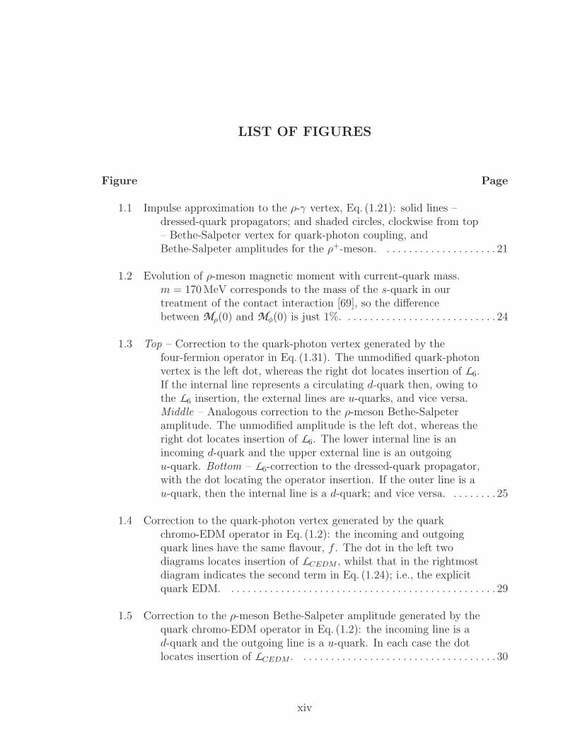
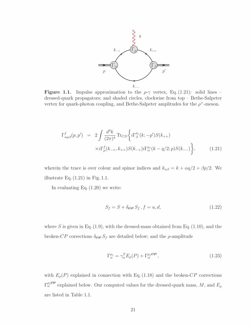
1.1 Impulse approximation to the ρ-γ vertex, Eq. (1.21): solid lines –dressed-quark propagators; and shaded circles, clockwise from top– Bethe-Salpeter vertex for quark-photon coupling, andBethe-Salpeter amplitudes for the ρ+-meson. . . . . . . . . . . . . . . . . . . . . 21
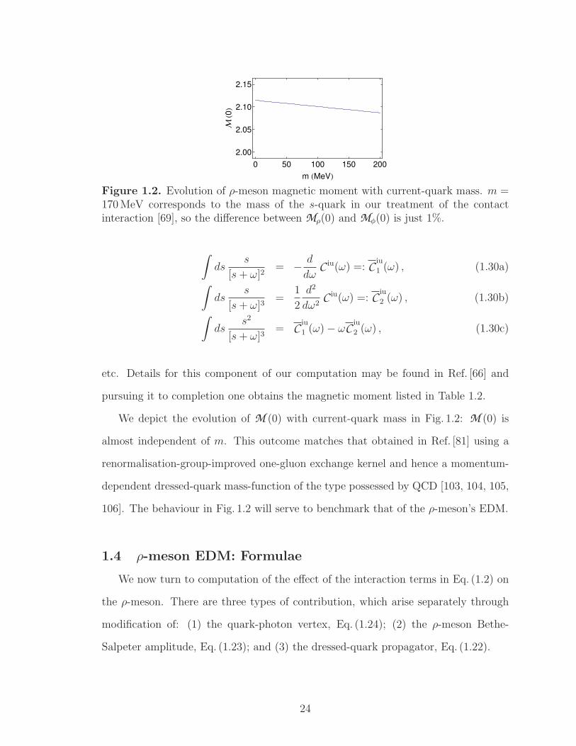
1.2 Evolution of ρ-meson magnetic moment with current-quark mass.m = 170 MeV corresponds to the mass of the s-quark in ourtreatment of the contact interaction [69], so the differencebetween Mρ(0) and Mφ(0) is just 1%. . . . . . . . . . . . . . . . . . . . . . . . . . . . 24
1.3 Top – Correction to the quark-photon vertex generated by thefour-fermion operator in Eq. (1.31). The unmodified quark-photonvertex is the left dot, whereas the right dot locates insertion of L6.If the internal line represents a circulating d-quark then, owing tothe L6 insertion, the external lines are u-quarks, and vice versa.Middle – Analogous correction to the ρ-meson Bethe-Salpeteramplitude. The unmodified amplitude is the left dot, whereas theright dot locates insertion of L6. The lower internal line is anincoming d-quark and the upper external line is an outgoingu-quark. Bottom – L6-correction to the dressed-quark propagator,with the dot locating the operator insertion. If the outer line is au-quark, then the internal line is a d-quark; and vice versa. . . . . . . . . 25
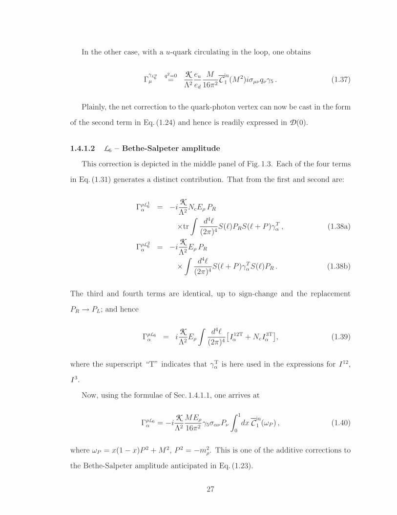
1.4 Correction to the quark-photon vertex generated by the quarkchromo-EDM operator in Eq. (1.2): the incoming and outgoingquark lines have the same flavour, f . The dot in the left twodiagrams locates insertion of LCEDM , whilst that in the rightmostdiagram indicates the second term in Eq. (1.24); i.e., the explicitquark EDM. . . . . . . . . . . . . . . . . . . . . . . . . . . . . . . . . . . . . . . . . . . . . . . . . 29
1.5 Correction to the ρ-meson Bethe-Salpeter amplitude generated by thequark chromo-EDM operator in Eq. (1.2): the incoming line is ad-quark and the outgoing line is a u-quark. In each case the dotlocates insertion of LCEDM . . . . . . . . . . . . . . . . . . . . . . . . . . . . . . . . . . . . 30
xiv
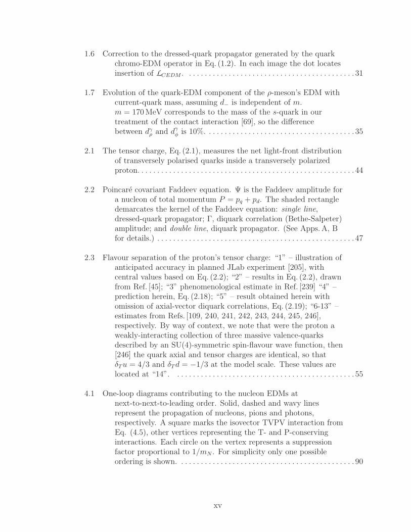
1.6 Correction to the dressed-quark propagator generated by the quarkchromo-EDM operator in Eq. (1.2). In each image the dot locatesinsertion of LCEDM . . . . . . . . . . . . . . . . . . . . . . . . . . . . . . . . . . . . . . . . . . . 31
1.7 Evolution of the quark-EDM component of the ρ-meson’s EDM withcurrent-quark mass, assuming d− is independent of m.m = 170 MeV corresponds to the mass of the s-quark in ourtreatment of the contact interaction [69], so the differencebetween dγ
ρ and dγφ is 10%. . . . . . . . . . . . . . . . . . . . . . . . . . . . . . . . . . . . . . 35
2.1 The tensor charge, Eq. (2.1), measures the net light-front distributionof transversely polarised quarks inside a transversely polarizedproton. . . . . . . . . . . . . . . . . . . . . . . . . . . . . . . . . . . . . . . . . . . . . . . . . . . . . . . 44
2.2 Poincare covariant Faddeev equation. Ψ is the Faddeev amplitude fora nucleon of total momentum P = pq + pd. The shaded rectangledemarcates the kernel of the Faddeev equation: single line,dressed-quark propagator; Γ, diquark correlation (Bethe-Salpeter)amplitude; and double line, diquark propagator. (See Apps. A, Bfor details.) . . . . . . . . . . . . . . . . . . . . . . . . . . . . . . . . . . . . . . . . . . . . . . . . . . 47
2.3 Flavour separation of the proton’s tensor charge: “1” – illustration ofanticipated accuracy in planned JLab experiment [205], withcentral values based on Eq. (2.2); “2” – results in Eq. (2.2), drawnfrom Ref. [45]; “3” phenomenological estimate in Ref. [239] “4” –prediction herein, Eq. (2.18); “5” – result obtained herein withomission of axial-vector diquark correlations, Eq. (2.19); “6-13” –estimates from Refs. [109, 240, 241, 242, 243, 244, 245, 246],respectively. By way of context, we note that were the proton aweakly-interacting collection of three massive valence-quarksdescribed by an SU(4)-symmetric spin-flavour wave function, then[246] the quark axial and tensor charges are identical, so thatδTu = 4/3 and δTd = −1/3 at the model scale. These values arelocated at “14”. . . . . . . . . . . . . . . . . . . . . . . . . . . . . . . . . . . . . . . . . . . . . . 55
4.1 One-loop diagrams contributing to the nucleon EDMs atnext-to-next-to-leading order. Solid, dashed and wavy linesrepresent the propagation of nucleons, pions and photons,respectively. A square marks the isovector TVPV interaction fromEq. (4.5), other vertices representing the T- and P-conservinginteractions. Each circle on the vertex represents a suppressionfactor proportional to 1/mN . For simplicity only one possibleordering is shown. . . . . . . . . . . . . . . . . . . . . . . . . . . . . . . . . . . . . . . . . . . . . 90
xv
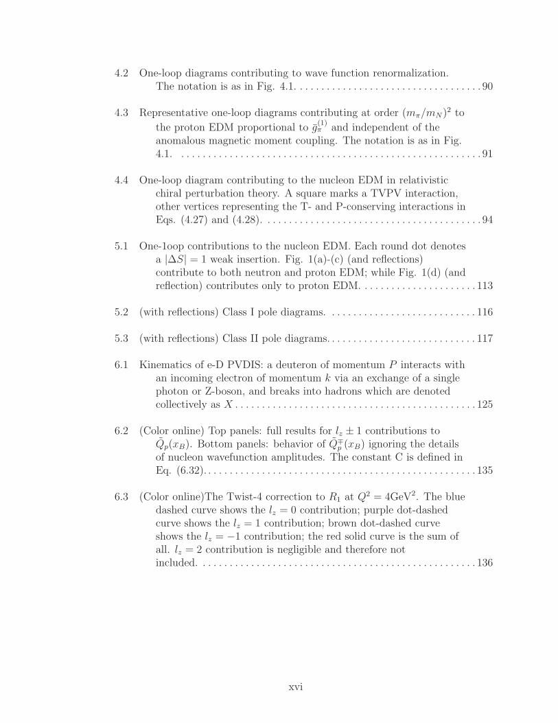
4.2 One-loop diagrams contributing to wave function renormalization.The notation is as in Fig. 4.1. . . . . . . . . . . . . . . . . . . . . . . . . . . . . . . . . . . 90
4.3 Representative one-loop diagrams contributing at order (mπ/mN)2 to
the proton EDM proportional to g(1)π and independent of the
anomalous magnetic moment coupling. The notation is as in Fig.4.1. . . . . . . . . . . . . . . . . . . . . . . . . . . . . . . . . . . . . . . . . . . . . . . . . . . . . . . . . 91
4.4 One-loop diagram contributing to the nucleon EDM in relativisticchiral perturbation theory. A square marks a TVPV interaction,other vertices representing the T- and P-conserving interactions inEqs. (4.27) and (4.28). . . . . . . . . . . . . . . . . . . . . . . . . . . . . . . . . . . . . . . . . 94
5.1 One-1oop contributions to the nucleon EDM. Each round dot denotesa |∆S| = 1 weak insertion. Fig. 1(a)-(c) (and reflections)contribute to both neutron and proton EDM; while Fig. 1(d) (andreflection) contributes only to proton EDM. . . . . . . . . . . . . . . . . . . . . . 113
5.2 (with reflections) Class I pole diagrams. . . . . . . . . . . . . . . . . . . . . . . . . . . . 116
5.3 (with reflections) Class II pole diagrams. . . . . . . . . . . . . . . . . . . . . . . . . . . . 117
6.1 Kinematics of e-D PVDIS: a deuteron of momentum P interacts withan incoming electron of momentum k via an exchange of a singlephoton or Z-boson, and breaks into hadrons which are denotedcollectively as X . . . . . . . . . . . . . . . . . . . . . . . . . . . . . . . . . . . . . . . . . . . . . 125
6.2 (Color online) Top panels: full results for lz ± 1 contributions toQp(xB). Bottom panels: behavior of Q∓
p (xB) ignoring the detailsof nucleon wavefunction amplitudes. The constant C is defined inEq. (6.32). . . . . . . . . . . . . . . . . . . . . . . . . . . . . . . . . . . . . . . . . . . . . . . . . . . 135
6.3 (Color online)The Twist-4 correction to R1 at Q2 = 4GeV2. The bluedashed curve shows the lz = 0 contribution; purple dot-dashedcurve shows the lz = 1 contribution; brown dot-dashed curveshows the lz = −1 contribution; the red solid curve is the sum ofall. lz = 2 contribution is negligible and therefore notincluded. . . . . . . . . . . . . . . . . . . . . . . . . . . . . . . . . . . . . . . . . . . . . . . . . . . . 136
xvi
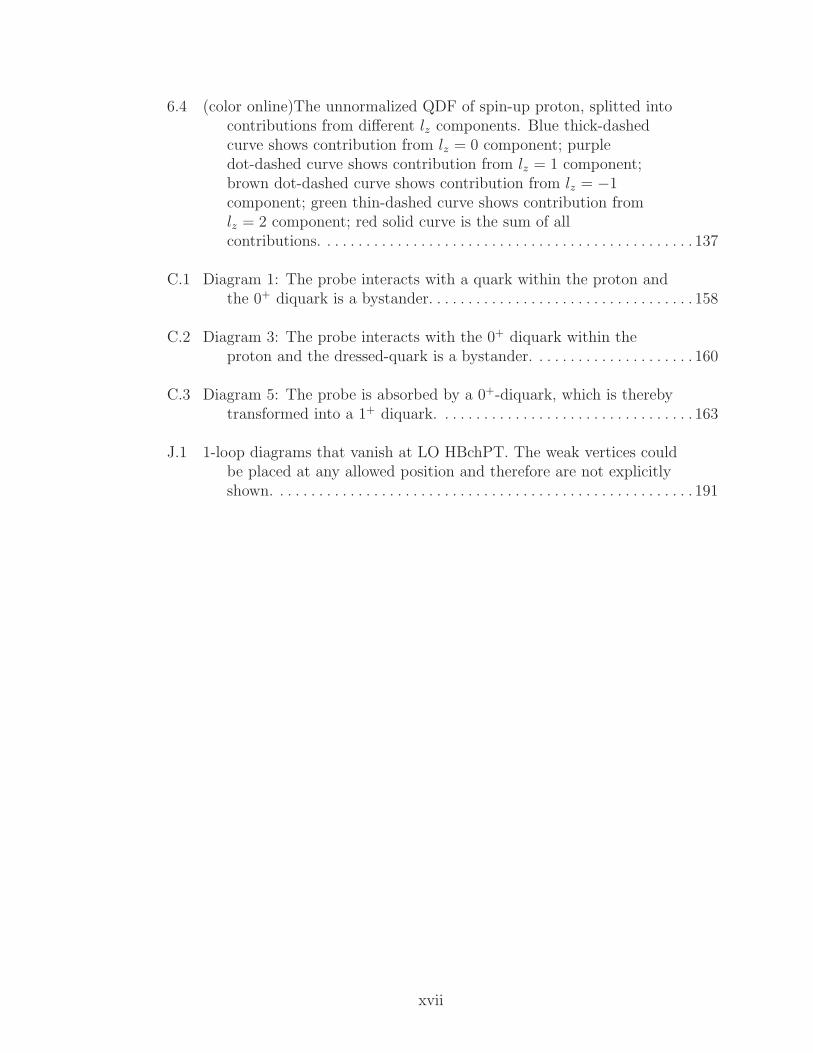
6.4 (color online)The unnormalized QDF of spin-up proton, splitted intocontributions from different lz components. Blue thick-dashedcurve shows contribution from lz = 0 component; purpledot-dashed curve shows contribution from lz = 1 component;brown dot-dashed curve shows contribution from lz = −1component; green thin-dashed curve shows contribution fromlz = 2 component; red solid curve is the sum of allcontributions. . . . . . . . . . . . . . . . . . . . . . . . . . . . . . . . . . . . . . . . . . . . . . . . 137
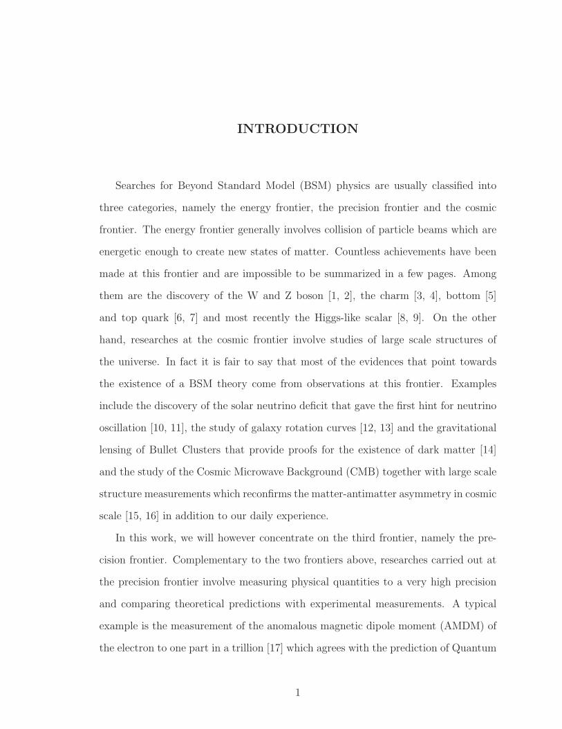
C.1 Diagram 1: The probe interacts with a quark within the proton andthe 0+ diquark is a bystander. . . . . . . . . . . . . . . . . . . . . . . . . . . . . . . . . . 158
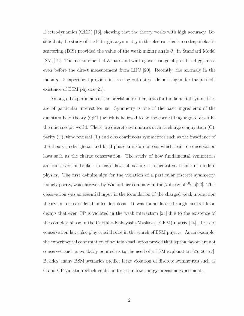
C.2 Diagram 3: The probe interacts with the 0+ diquark within theproton and the dressed-quark is a bystander. . . . . . . . . . . . . . . . . . . . . 160
C.3 Diagram 5: The probe is absorbed by a 0+-diquark, which is therebytransformed into a 1+ diquark. . . . . . . . . . . . . . . . . . . . . . . . . . . . . . . . . 163
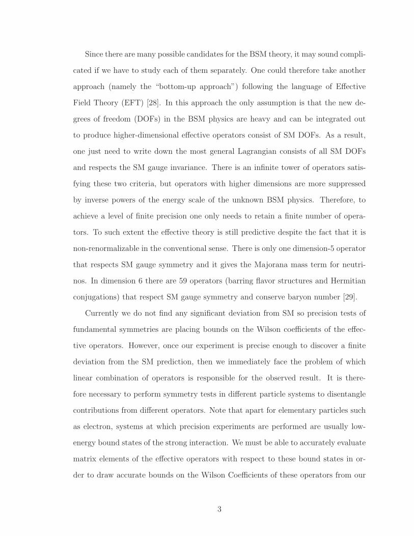
J.1 1-loop diagrams that vanish at LO HBchPT. The weak vertices couldbe placed at any allowed position and therefore are not explicitlyshown. . . . . . . . . . . . . . . . . . . . . . . . . . . . . . . . . . . . . . . . . . . . . . . . . . . . . . 191
xvii
INTRODUCTION
Searches for Beyond Standard Model (BSM) physics are usually classified into
three categories, namely the energy frontier, the precision frontier and the cosmic
frontier. The energy frontier generally involves collision of particle beams which are
energetic enough to create new states of matter. Countless achievements have been
made at this frontier and are impossible to be summarized in a few pages. Among
them are the discovery of the W and Z boson [1, 2], the charm [3, 4], bottom [5]
and top quark [6, 7] and most recently the Higgs-like scalar [8, 9]. On the other
hand, researches at the cosmic frontier involve studies of large scale structures of
the universe. In fact it is fair to say that most of the evidences that point towards
the existence of a BSM theory come from observations at this frontier. Examples
include the discovery of the solar neutrino deficit that gave the first hint for neutrino
oscillation [10, 11], the study of galaxy rotation curves [12, 13] and the gravitational
lensing of Bullet Clusters that provide proofs for the existence of dark matter [14]
and the study of the Cosmic Microwave Background (CMB) together with large scale
structure measurements which reconfirms the matter-antimatter asymmetry in cosmic
scale [15, 16] in addition to our daily experience.
In this work, we will however concentrate on the third frontier, namely the pre-
cision frontier. Complementary to the two frontiers above, researches carried out at
the precision frontier involve measuring physical quantities to a very high precision
and comparing theoretical predictions with experimental measurements. A typical
example is the measurement of the anomalous magnetic dipole moment (AMDM) of
the electron to one part in a trillion [17] which agrees with the prediction of Quantum
1
Electrodynamics (QED) [18], showing that the theory works with high accuracy. Be-
side that, the study of the left-right asymmetry in the electron-deuteron deep inelastic
scattering (DIS) provided the value of the weak mixing angle θw in Standard Model
(SM)[19]. The measurement of Z-mass and width gave a range of possible Higgs mass
even before the direct measurement from LHC [20]. Recently, the anomaly in the
muon g−2 experiment provides interesting but not yet definite signal for the possible
existence of BSM physics [21].
Among all experiments at the precision frontier, tests for fundamental symmetries
are of particular interest for us. Symmetry is one of the basic ingredients of the
quantum field theory (QFT) which is believed to be the correct language to describe
the microscopic world. There are discrete symmetries such as charge conjugation (C),
parity (P), time reversal (T) and also continuous symmetries such as the invariance of
the theory under global and local phase transformations which lead to conservation
laws such as the charge conservation. The study of how fundamental symmetries
are conserved or broken in basic laws of nature is a persistent theme in modern
physics. The first definite sign for the violation of a particular discrete symmetry,
namely parity, was observed by Wu and her company in the β-decay of 60Co[22]. This
observation was an essential input in the formulation of the charged weak interaction
theory in terms of left-handed fermions. It was found later through neutral kaon
decays that even CP is violated in the weak interaction [23] due to the existence of
the complex phase in the Cabibbo-Kobayashi-Maskawa (CKM) matrix [24]. Tests of
conservation laws also play crucial roles in the search of BSM physics. As an example,
the experimental confirmation of neutrino oscillation proved that lepton flavors are not
conserved and unavoidably pointed us to the need of a BSM explanation [25, 26, 27].
Besides, many BSM scenarios predict large violation of discrete symmetries such as
C and CP-violation which could be tested in low energy precision experiments.
2
Since there are many possible candidates for the BSM theory, it may sound compli-
cated if we have to study each of them separately. One could therefore take another
approach (namely the “bottom-up approach”) following the language of Effective
Field Theory (EFT) [28]. In this approach the only assumption is that the new de-
grees of freedom (DOFs) in the BSM physics are heavy and can be integrated out
to produce higher-dimensional effective operators consist of SM DOFs. As a result,
one just need to write down the most general Lagrangian consists of all SM DOFs
and respects the SM gauge invariance. There is an infinite tower of operators satis-
fying these two criteria, but operators with higher dimensions are more suppressed
by inverse powers of the energy scale of the unknown BSM physics. Therefore, to
achieve a level of finite precision one only needs to retain a finite number of opera-
tors. To such extent the effective theory is still predictive despite the fact that it is
non-renormalizable in the conventional sense. There is only one dimension-5 operator
that respects SM gauge symmetry and it gives the Majorana mass term for neutri-
nos. In dimension 6 there are 59 operators (barring flavor structures and Hermitian
conjugations) that respect SM gauge symmetry and conserve baryon number [29].
Currently we do not find any significant deviation from SM so precision tests of
fundamental symmetries are placing bounds on the Wilson coefficients of the effec-
tive operators. However, once our experiment is precise enough to discover a finite
deviation from the SM prediction, then we immediately face the problem of which
linear combination of operators is responsible for the observed result. It is there-
fore necessary to perform symmetry tests in different particle systems to disentangle
contributions from different operators. Note that apart for elementary particles such
as electron, systems at which precision experiments are performed are usually low-
energy bound states of the strong interaction. We must be able to accurately evaluate
matrix elements of the effective operators with respect to these bound states in or-
der to draw accurate bounds on the Wilson Coefficients of these operators from our
3
results of precision experiments. However, when we try to proceed in this direction
we immediately run into the difficulty in performing analytic calculations involving
bound states of the strong interaction from first principle.
Quantum Chromodynamics (QCD) is a gauge theory that describes the strong
interaction between quarks through the exchange of gluons which are SU(3)C gauge
bosons. Even though there are many evidences that it is indeed the correct the-
ory of the strong interaction, only very limited analytical results using perturbation
theory at high energy can be derived from first principle, thank to its asymptotically-
free behavior at high energy [30, 31]. On the other hand, the theory becomes non-
perturbative at energy < 1 GeV so the conventional perturbation theory based on the
expansion in powers of the strong coupling constant αs fails. Some very interesting
emergent features of theory in this energy regime such as confinement and dynamical
chiral symmetry breaking (DCSB) are still not well understood. Although lattice
QCD [32] provides a promising way to extract numerical results from first principle
calculations, but it is subject to numerous technical difficulties and therefore has a
limited range of application. Furthermore, not just satisfied by just obtaining numeri-
cal answers, we need a more intuitive understanding of how low-energy QCD behaves.
For the latter purpose and also practical reasons, many effective approaches to low
energy QCD are formulated that allow studies of hadronic or nuclear properties, and
each of them tries to capture some known behaviors of the original theory such as
confinement and chiral symmetry breaking. Among them are the Chiral Perturbation
Theory (ChPT), constituent quark model, Regge Theory, Dyson-Schwinger Equation
(DSE), QCD sum rules and others.
We have two main tasks in this work. On the one hand, we will introduce a number
of effective approaches to QCD which allow us to perform analytical and numerical
studies of both static and dynamical properties of hadrons. On the other hand, we will
apply these effective approaches in the calculation of hadronic matrix elements and the
4
determination of specific SM backgrounds that enter various precision experiments in
tests of fundamental symmetries. In particular, we will concentrate on EDM searches
in hadrons, precision experiments involving the neutron β-decay and the study of
P-violation in the electron-deuteron parity-violating deep inelastic scattering (e-D
PVDIS).
EDMs And Hadronic Matrix Elements
Ever since the discovery of P-violation in the weak interaction, people are puzzled
by the fact that discrete symmetries such as P and CP are violated only in the weak
interaction and not in other interactions. Various experiments have been carried out
to test the conservation of these discrete symmetries in strong and electromagnetic
sector. Back in the 50s, Smith, Purcell and Ramsey had suggested the test of P-
invariance in the strong interaction by searching for intrinsic electric dipole moment
(EDM) of the neutron [33]. Since then, experimental techniques have improved much
and searches of permanent EDMs in different particle systems have been carried out
but so far all of them have returned null results. This raised another interesting
question known as the strong CP-problem, namely: due to the non-trivial vacuum
structure of QCD, one can write down a term in the Lagrangian which is P and CP-
violating and is characterized by the parameter θ. In general there is no constraint
on the value of θ by the theory itself so it could be of order one by naturalness.
However, the (so-far) vanishing of EDMs in all hadronic systems indicates that the
value of θ has to be fine-tuned to an extremely small number, which makes the whole
theory seems unnatural. There have been several proposed solution to this problem.
Among them are the massless up quark solution [34], the Peccei-Quinn symmetry [35]
and the Nelson-Barr mechanism [36, 37] but so far none of them seems completely
satisfactory.
5
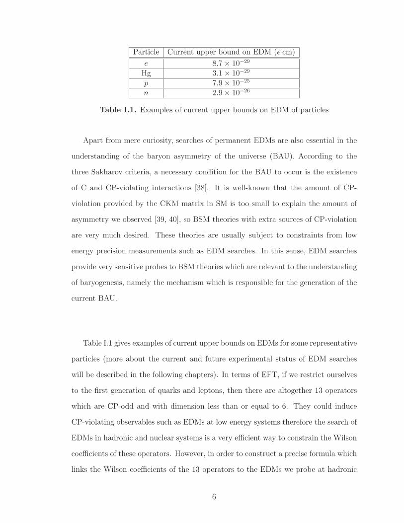
Particle Current upper bound on EDM (e cm)
e 8.7 × 10⁻²⁹
Hg 3.1 × 10⁻²⁹
p 7.9 × 10⁻²⁵
n 2.9 × 10⁻²⁶
Table I.1. Examples of current upper bounds on EDM of particles
Apart from mere curiosity, searches of permanent EDMs are also essential in the
understanding of the baryon asymmetry of the universe (BAU). According to the
three Sakharov criteria, a necessary condition for the BAU to occur is the existence
of C and CP-violating interactions [38]. It is well-known that the amount of CP-
violation provided by the CKM matrix in SM is too small to explain the amount of
asymmetry we observed [39, 40], so BSM theories with extra sources of CP-violation
are very much desired. These theories are usually subject to constraints from low
energy precision measurements such as EDM searches. In this sense, EDM searches
provide very sensitive probes to BSM theories which are relevant to the understanding
of baryogenesis, namely the mechanism which is responsible for the generation of the
current BAU.
Table I.1 gives examples of current upper bounds on EDMs for some representative
particles (more about the current and future experimental status of EDM searches
will be described in the following chapters). In terms of EFT, if we restrict ourselves
to the first generation of quarks and leptons, then there are altogether 13 operators
which are CP-odd and with dimension less than or equal to 6. They could induce
CP-violating observables such as EDMs at low energy systems therefore the search of
EDMs in hadronic and nuclear systems is a very efficient way to constrain the Wilson
coefficients of these operators. However, in order to construct a precise formula which
links the Wilson coefficients of the 13 operators to the EDMs we probe at hadronic
6
systems we must be able to reduce the theoretical uncertainty in the calculation of
relevant hadronic matrix elements.
In this work we will present several case studies on EDMs induced by BSM physics
in different hadronic systems. First we will work with the ρ-meson which is the
simplest possible hadron that could possess an EDM. The aim of this work is to
find a single framework that can deal with the hadronic matrix elements of different
sources of CP-violation in a unified and coherent manner. We will show that the
Dyson-Schwinger Equation is good choice for this purpose. Within the framework
of DSE we will compute the ρ-EDM induced by the quark EDM, the quark chromo-
EDM, the QCD θ-term and the four quark operator (which covers most operators
of P and CP-violation up to dimension 6). This work shall serve as a prototype for
future studies of more realistic systems such as nucleon within the same theoretical
framework.
On the other hand, it is known that a significant amount of BSM-induced nucleon
EDM enters in the form of long-distance contribution, namely the contribution via
effective P and CP-odd pion-nucleon couplings. Chiral Perturbation Theory provides
a model-independent description of the properties of QCD in this regime as it is
simply the most general theory at low energy which is consistent with the exact
and approximate symmetries of QCD. With the aid of ChPT we will perform an
investigation on the pion loop correction to the nucleon EDM induced by the P and
T-odd pion-nucleon coupling g(i)π .
Finally, we would like to mention that although it is commonly understood that
SM-induced EDMs are too small to be observed with the current experimental preci-
sion, it is still worth a detailed study since the complex phase in the CKM matrix is
currently the only experimentally-confirmed source of CP-violation in nature. For this
purpose we will also present an updated work on the SM-induced nucleon EDM. We
will show that previous studies on this topic were based on a flawed effective theory
7
of hadrons that does not posses a valid expansion scheme at low energy. Also, their
results face large uncertainties due to poorly known physical constants in the weak
sector at that time. Our updated study will try to fix these two problems and obtain
a better determination of the nucleon EDM with a smaller theoretical uncertainty.
Scalar And Tensor Charges In The Neutron β-Decay
The β-decay of nuclei became an excellent playground for the test of fundamental
symmetries since the discovery of parity violation in the β-decay of 60Co which led
eventually to the V-A structure of the charged weak interaction. Recently nuclear
β-decays have been studied extensively for the purpose of BSM searches [41]. In
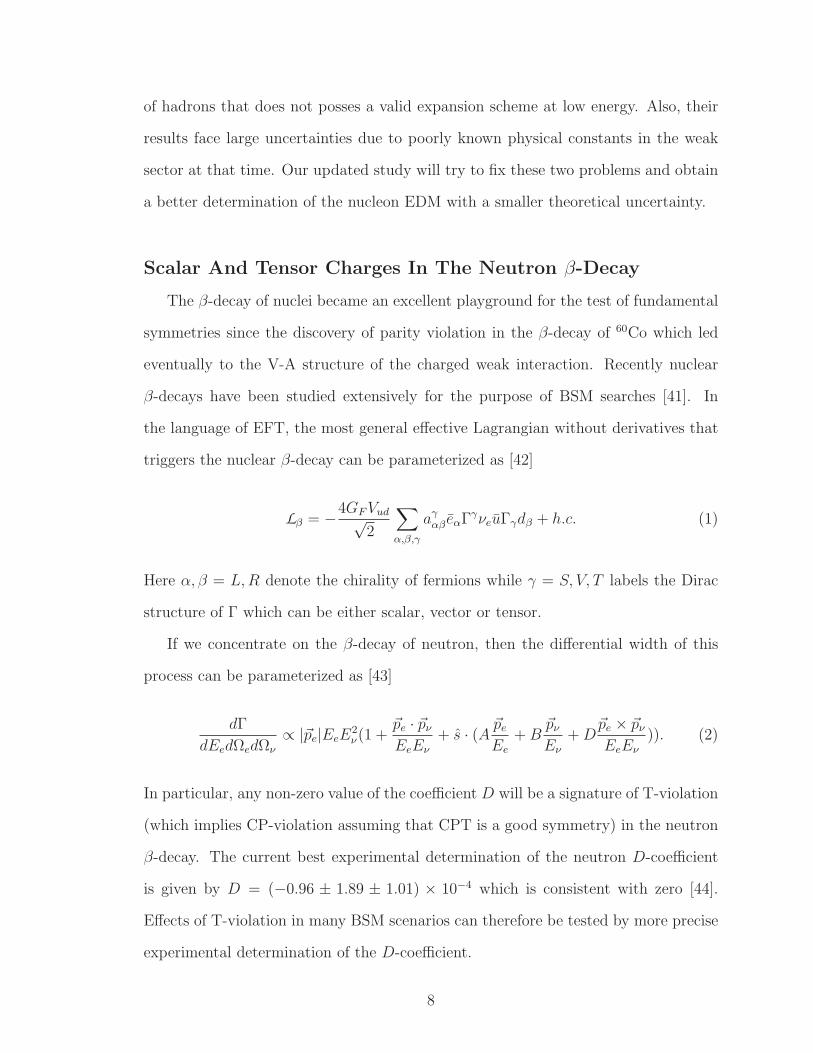
the language of EFT, the most general effective Lagrangian without derivatives that
triggers the nuclear β-decay can be parameterized as [42]
Lβ = −4GFVud√2
∑
α,β,γ
aγαβ eαΓγνeuΓγdβ + h.c. (1)
Here α, β = L,R denote the chirality of fermions while γ = S, V, T labels the Dirac
structure of Γ which can be either scalar, vector or tensor.
If we concentrate on the β-decay of neutron, then the differential width of this
process can be parameterized as [43]
dΓ
dEedΩedΩν
∝ |~pe|EeE2ν(1 +
~pe · ~pν
EeEν
+ s · (A ~pe
Ee
+B~pν
Eν
+D~pe × ~pν
EeEν
)). (2)
In particular, any non-zero value of the coefficient D will be a signature of T-violation
(which implies CP-violation assuming that CPT is a good symmetry) in the neutron
β-decay. The current best experimental determination of the neutron D-coefficient
is given by D = (−0.96 ± 1.89 ± 1.01) × 10−4 which is consistent with zero [44].
Effects of T-violation in many BSM scenarios can therefore be tested by more precise
experimental determination of the D-coefficient.
8
In terms of the parametrization in Eq. (1), the value of D is related to the
imaginary part of aγαβ which depends on the specific BSM realization. However the
application of Eq. (1) in the computation of the neutron D-coefficient given in Eq.
(2) requires the evaluation of the hadronic matrix element 〈p| uαΓγdβ |n〉 at small
momentum transfer. When γ = V , the relevant matrix elements are called the vector
(gV ) and axial (gA) charges. They can be determined quite precisely by experiment.
On the other hand, when γ = S or T the corresponding hadronic matrix elements
are called scalar (gS) and tensor (gT ) charges respectively. The current experimental
values of these charges suffer from very large uncertainty [45] so theoretical modelings
are needed.
We will present a calculation of the nucleon scalar and tensor charges using the
Dyson-Schwinger Equation formalism with a simplified vector-like interaction be-
tween quarks. This simplified model has been shown to give identical results with
more sophisticated truncation schemes of DSE when dealing with static behaviors of
hadrons. The application of this formalism allows us to compute hadronic matrix
elements using the conventional Feynman diagram approach with dressed propaga-
tors and vertices while only very little amount of numerical calculation is required.
In particular, we will show that the inclusion of an axial-like diquark correlation in
the nucleon is essential to reproduce a nucleon tensor charge that falls within current
range of uncertainty of the current experiment. This work therefore contributes to
both the search of BSM physics and also the understanding of quark correlations in
the nucleon.
Higher-Twist Correction And The Study of Nucleon Spin In
Parity-Violating Deep Inelastic Scattering
A good way to study the parity violation in the weak interaction is to perform
deep inelastic scattering between on the deuteron target with longitudinally-polarized
9
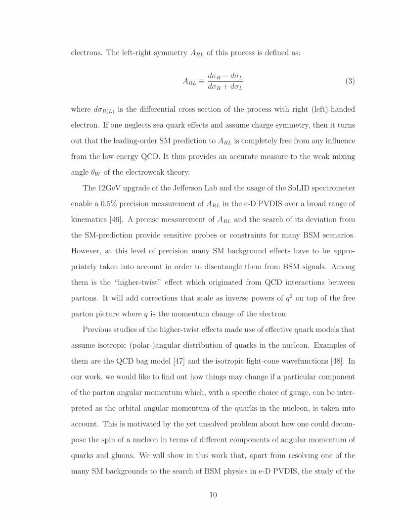
electrons. The left-right symmetry ARL of this process is defined as:
ARL ≡ dσR − dσL
dσR + dσL
(3)
where dσR(L) is the differential cross section of the process with right (left)-handed
electron. If one neglects sea quark effects and assume charge symmetry, then it turns
out that the leading-order SM prediction to ARL is completely free from any influence
from the low energy QCD. It thus provides an accurate measure to the weak mixing
angle θW of the electroweak theory.
The 12GeV upgrade of the Jefferson Lab and the usage of the SoLID spectrometer
enable a 0.5% precision measurement of ARL in the e-D PVDIS over a broad range of
kinematics [46]. A precise measurement of ARL and the search of its deviation from
the SM-prediction provide sensitive probes or constraints for many BSM scenarios.
However, at this level of precision many SM background effects have to be appro-
priately taken into account in order to disentangle them from BSM signals. Among
them is the “higher-twist” effect which originated from QCD interactions between
partons. It will add corrections that scale as inverse powers of q2 on top of the free
parton picture where q is the momentum change of the electron.
Previous studies of the higher-twist effects made use of effective quark models that
assume isotropic (polar-)angular distribution of quarks in the nucleon. Examples of
them are the QCD bag model [47] and the isotropic light-cone wavefunctions [48]. In
our work, we would like to find out how things may change if a particular component
of the parton angular momentum which, with a specific choice of gauge, can be inter-
preted as the orbital angular momentum of the quarks in the nucleon, is taken into
account. This is motivated by the yet unsolved problem about how one could decom-
pose the spin of a nucleon in terms of different components of angular momentum of
quarks and gluons. We will show in this work that, apart from resolving one of the
many SM backgrounds to the search of BSM physics in e-D PVDIS, the study of the
10
higher-twist matrix element is interesting by itself as it sheds new lights on the study
of the rule of angular momentum in the structure of the nucleon.
The Arrangement Of The Contents
The contents of this thesis are arranged as follows: in Chapter 1 I will provide
a brief introduction to the Dyson-Schwinger Equation and describe the “contact-
interaction” approximation and apply the DSE formalism to compute the EDM of the
ρ-meson induced by various CP-violating effective operators. In Chapter 2 I apply the
same formalism in the calculation of the scalar and tensor charges of the nucleon. In
Chapter 3 I will introduce some essential concepts of the Chiral Perturbation Theory
and its heavy baryon reduction. In Chapter 4 I apply the two-flavor ChPT to compute
the nucleon EDM induced by the P,T-odd pion-nucleon coupling. In Chapter 5 I will
apply the three-flavor ChPT to study the SM-induced nucleon EDMs. In Chapter 6
I study the higher-twist correction to the e-D PVDIS and draw connections with the
nucleon spin problem. In the last chapter I will present some general discussions and
draw my conclusions.
11
CHAPTER 1
ELECTRIC DIPOLE MOMENT OF THE ρ-MESON
1.1 Introduction
The action for any local quantum field theory is invariant under the transformation
generated by the antiunitary operator CPT , which is the product of the inversions:
C, charge conjugation; P , parity transformation; and T , time reversal. The combined
CPT transformation provides a rigorous correspondence between particles and an-
tiparticles, and it relates the S matrix for any given process to its inverse, where all
spins are flipped and the particles replaced by their antiparticles. Lorentz and CPT
symmetry together have many consequences, amongst them, that the mass and total
width of any particle are identical to those of its antiparticle.
It is within this context that the search for the intrinsic electric dipole moment
(EDM) of an elementary or composite but fundamental particle has held the fasci-
nation of physicists for over sixty years [49]. Its existence indicates the simultaneous
violation of parity- and time-reversal-invariance in the theory that describes the par-
ticle’s structure and interactions; and the violation of P - and T -invariance entails
that CP symmetry is also broken. This last is critical for our existence because
we represent a macroscopic excess of matter over antimatter. As first observed by
Sakharov [38], in order for a theory to explain an excess of baryon matter, it must
include processes that change baryon number, and break C- and CP -symmetries;
0Reprinted article with permission from M. Pitschmann, C. Y. Seng, M. J. Ramsey-Musolf,C. D. Roberts, S. M. Schmidt and D. J. Wilson, Phys. Rev. C 87 (2013) no.1, 015205, Copyright(2013) by the American Physical Society. DOI: http://dx.doi.org/10.1103/PhysRevC.87.015205
12
and the relevant processes must have taken place out of equilibrium, otherwise they
would merely have balanced matter and antimatter. (Alternately, the presence of
CPT violation can circumvent the out-of-equilibrium environment.)
The electroweak component of the Standard Model (SM) is capable of satisfying
Sakharov’s conditions, owing to the existence of a complex phase in the 3 × 3-CKM
matrix which enables processes that mix all three quark generations. However, this
high-order process is too weak to explain the observed matter-antimatter asymmetry
[50, 51, 52]. Hence, it is widely expected that any description of baryogenesis will
require new sources of CP violation beyond the SM. This presents little difficulty,
however, because extensions of the SM typically possess CP -violating interactions,
whose parameters must, in fact, be tuned to small values in order to avoid conflict
with known bounds on the size of such EDMs [52, 53, 54, 55, 56]. (For recent analyses,
see, e.g., Refs. [57, 58, 59] and references therein.)
The question here is how such bounds should be imposed. That is not a problem
for elementary particles, like the electron. However, it is a challenge when the SM
extension produces an operator involving current-quarks and/or gluons. In that case
the CP violation is expressed as an hadronic property and one must have at hand a
nonperturbative method with which to compute the impact of CP -violating features
of partonic quarks and gluons on the hadronic composite.
To elucidate, extensions of the SM are typically active at some large but unspeci-
fied energy-scale, Λ, and their effect at an hadronic scale is expressed in a low-energy
effective Lagrangian:
Leff ∼∑
j,k
Kj O(k)j Λ4−k, (1.1)
where O(k)j are composite CP -odd local operators of dimension k ≥ 4 and Kj
are dimensionless strength parameters, which monitor the size of the model’s CP -
violating phases and commonly evolve logarithmically with the energy scale. The
calculation of an hadronic EDM therefore proceeds in two steps. The first, easier,
13
part requires calculation of the coefficients Ki in a given model. This involves the
systematic elimination of degrees-of-freedom that are irrelevant at energy-scales less
than Λ. The second, far more challenging exercise, is the nonperturbative problem of
translating the current-quark-level interaction in Eq. (1.1) into observable properties
of hadrons.
We illustrate the procedure in the case of the ρ-meson. Not that there is any hope
of measuring a ρ-meson EDM but because the nonperturbative methods necessary
can most readily be illustrated in the case of systems defined by two valence-quark
degrees-of-freedom. In taking this path, we follow other authors [60, 61, 62] but
will nonetheless expose novel insights, especially because we consider more operator
structures than have previously been considered within a single unifying framework.
It is worth remarking here that particles with spin also possess a magnetic dipole
moment. That moment is aligned with the particle’s spin because it is the only
vector available. The same is true of the expectation value of any electric dipole
moment.
Herein we shall estimate the contribution of some dimension four, five and six op-
erators to the EDM of the ρ+-meson; viz., the impact on the ρ of the local Lagrangian
density
Leff = −iθ g2s
32π2Ga
µνGaµν −
i
2
∑
q=u,d
dq q γ5σµνq Fµν
− i
2
∑
q=u,d
dq q12λ
aγ5σµνq gsGaµν +
K
Λ2iεjk
[
Qjd Qkγ5u+ h.c.]
, (1.2)
where: latin superscripts represent colour; gs is the strong coupling constant; Fµν and
Gaµν are photon and gluon field-strength tensors, respectively, and Ga
µν = (1/2)ǫµνλρGaλρ;
Qi|i = 1, 2 = uL, dL, with the subscript indicating left-handed; θ is QCD’s effec-
tive θ-parameter, which combines θQCD and the unknown phase of the current-quark-
mass matrix; and dq, dq are quark EDMs and chromo-EDMs, respectively.
14
We note that Eq. (1.2) is expressed at a renormalisation scale ζ ∼ 2 GeV, which
is far below that of electroweak symmetry breaking but still within the domain upon
which perturbative QCD is applicable. Moreover, we have chosen to include just
one dimension-six operator in the Lagrangian; i.e., a particular type of four-fermion
interaction. There is a host of dimension-six operators, Weinberg’s CP-odd three-
gluon vertex amongst them [63]. However, for our illustrative purpose, nothing is lost
by omitting them because the potency of the one operator we do consider can serve
as an indication of the strength with which each might contribute.
One merit of our analysis of the contribution from Eq. (1.2) to the EDM of the
ρ+-meson is the connection of these EDM responses with values of a vast array of
hadron observables that are all computed within precisely the same framework using
exactly the same parameters [64, 65, 66, 67, 68, 69]. We explain this framework in
Sec. 1.2. In addition to providing the first such comprehensive treatment, our study is
novel in considering the impact of a dimension-six operator on the ρ+-meson’s EDM.
We introduce the ρ-meson electromagnetic form factors in Sec. 1.3. The effects
of Eq. (1.2) on the ρ-meson bound-state are analysed in Sec. 1.4. Each interaction
term is considered separately, so that we present a raft of algebraic formulae that
are readily combined, evaluated and interpreted. Numerical results are provided in
Sec. 1.5 and placed in context with previous studies. Section 1.6 is an epilogue.
1.2 ρ-meson as a Bound State
1.2.1 ρ-γ Vertex
The ρ+-meson is a composite particle and thus its EDM appears in the dressed
vertex that describes its coupling with the photon; viz.,
15
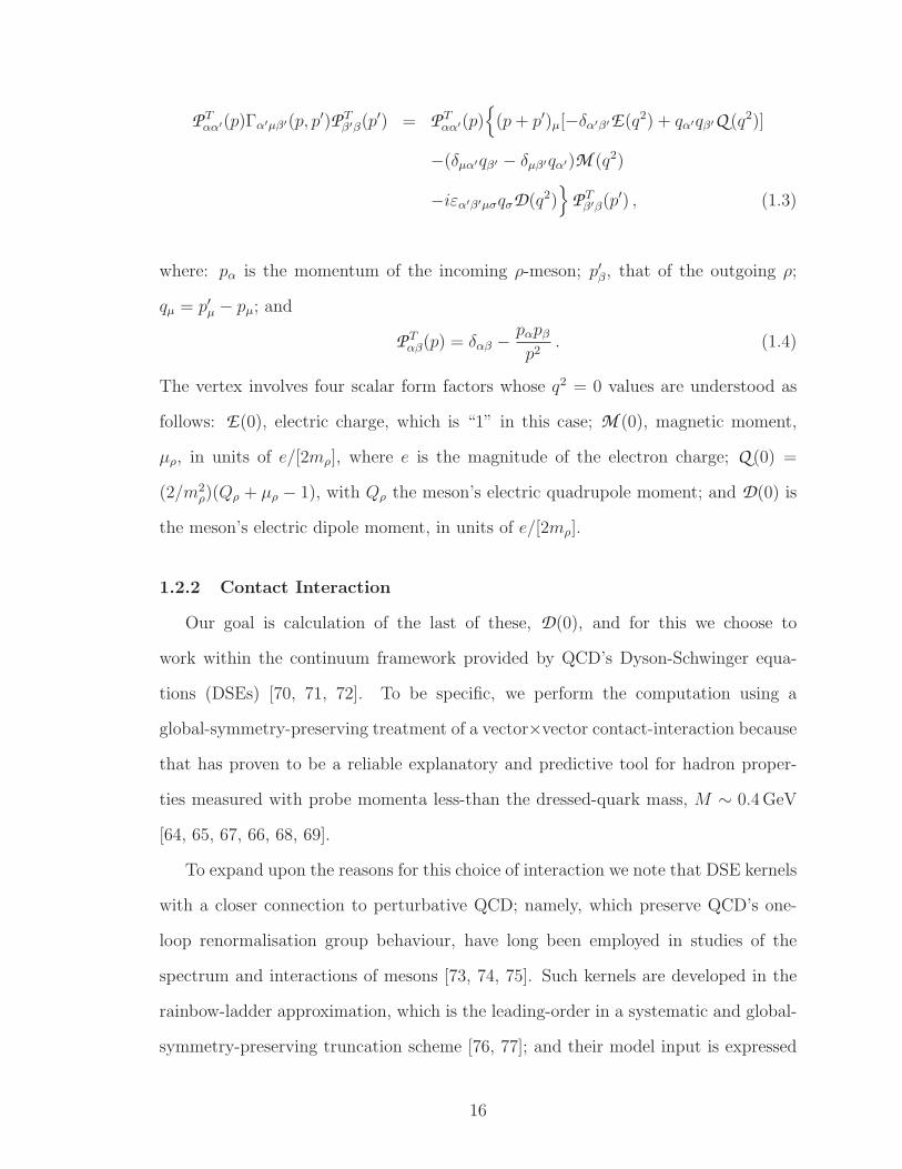
P Tαα′(p)Γα′µβ′(p, p′)P T
β′β(p′) = P Tαα′(p)
(p+ p′)µ[−δα′β′E(q2) + qα′qβ′Q (q2)]
−(δµα′qβ′ − δµβ′qα′)M (q2)
−iεα′β′µσqσD(q2)
P Tβ′β(p′) , (1.3)
where: pα is the momentum of the incoming ρ-meson; p′β, that of the outgoing ρ;
qµ = p′µ − pµ; and
P Tαβ(p) = δαβ − pαpβ
p2. (1.4)
The vertex involves four scalar form factors whose q2 = 0 values are understood as
follows: E(0), electric charge, which is “1” in this case; M (0), magnetic moment,
µρ, in units of e/[2mρ], where e is the magnitude of the electron charge; Q (0) =
(2/m2ρ)(Qρ + µρ − 1), with Qρ the meson’s electric quadrupole moment; and D(0) is
the meson’s electric dipole moment, in units of e/[2mρ].
1.2.2 Contact Interaction
Our goal is calculation of the last of these, D(0), and for this we choose to
work within the continuum framework provided by QCD’s Dyson-Schwinger equa-
tions (DSEs) [70, 71, 72]. To be specific, we perform the computation using a
global-symmetry-preserving treatment of a vector×vector contact-interaction because
that has proven to be a reliable explanatory and predictive tool for hadron proper-
ties measured with probe momenta less-than the dressed-quark mass, M ∼ 0.4 GeV
[64, 65, 67, 66, 68, 69].
To expand upon the reasons for this choice of interaction we note that DSE kernels
with a closer connection to perturbative QCD; namely, which preserve QCD’s one-
loop renormalisation group behaviour, have long been employed in studies of the
spectrum and interactions of mesons [73, 74, 75]. Such kernels are developed in the
rainbow-ladder approximation, which is the leading-order in a systematic and global-
symmetry-preserving truncation scheme [76, 77]; and their model input is expressed
16
via a statement about the nature of the gap equation’s kernel at infrared momenta.
With a single parameter that expresses a confinement length-scale or strength [78,
79], they have successfully described and predicted numerous properties of vector
[79, 80, 81, 82, 83] and pseudoscalar mesons [79, 82, 83, 84, 85, 86, 87] with masses
less than 1 GeV, and ground-state baryons [88, 89, 90, 91]. Such kernels are also
reliable for ground-state heavy-heavy mesons [92]. Given that contact-interaction
results for low-energy observables are indistinguishable from those produced by the
most sophisticated interactions, it is sensible to capitalise on the simplicity of the
contact-interaction herein.
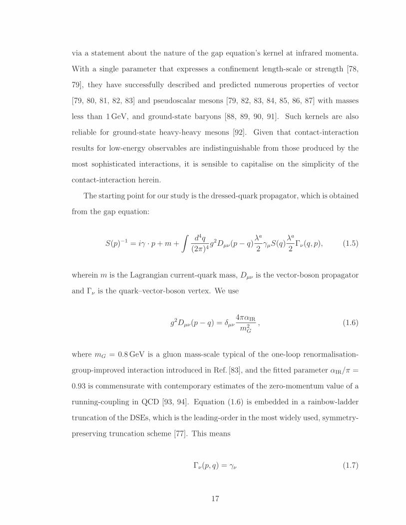
The starting point for our study is the dressed-quark propagator, which is obtained
from the gap equation:
S(p)−1 = iγ · p+m+
∫
d4q
(2π)4g2Dµν(p− q)
λa
2γµS(q)
λa
2Γν(q, p), (1.5)
wherein m is the Lagrangian current-quark mass, Dµν is the vector-boson propagator
and Γν is the quark–vector-boson vertex. We use
g2Dµν(p− q) = δµν4παIR
m2G
, (1.6)
where mG = 0.8 GeV is a gluon mass-scale typical of the one-loop renormalisation-
group-improved interaction introduced in Ref. [83], and the fitted parameter αIR/π =
0.93 is commensurate with contemporary estimates of the zero-momentum value of a
running-coupling in QCD [93, 94]. Equation (1.6) is embedded in a rainbow-ladder
truncation of the DSEs, which is the leading-order in the most widely used, symmetry-
preserving truncation scheme [77]. This means
Γν(p, q) = γν (1.7)
17

in Eq. (1.5) and in the subsequent construction of the Bethe-Salpeter kernels. One
may view the interaction in Eq. (1.6) as being inspired by models of the Nambu–Jona-
Lasinio (NJL) type [95]. However, in implementing the interaction as an element in
a rainbow-ladder truncation of the DSEs, our treatment is atypical; e.g., we have a
single, unique coupling parameter, whereas common applications of the NJL model
have different, tunable strength parameters for each collection of operators that mix
under symmetry transformations.
Using Eqs. (1.6), (1.7), the gap equation becomes
S−1(p) = iγ · p+m+16π
3
αIR
m2G
∫
d4q
(2π)4γµ S(q) γµ , (1.8)
an equation in which the integral possesses a quadratic divergence, even in the chiral
limit. When the divergence is regularised in a Poincare covariant manner, the solution
is
S(p)−1 = iγ · p+M , (1.9)
where M is momentum-independent and determined by
M = m+M4αIR
3πm2G
∫ ∞
0
ds s1
s+M2. (1.10)
Our regularisation procedure follows Ref. [96]; i.e., we write
1
s+M2=
∫ ∞
0
dτ e−τ(s+M2)
→∫ τ2
ir
τ2uv
dτ e−τ(s+M2) (1.11)
=e−(s+M2)τ2
uv − e−(s+M2)τ2ir
s+M2, (1.12)
where τir,uv are, respectively, infrared and ultraviolet regulators. It is apparent from
Eq. (1.12) that τir =: 1/Λir finite implements confinement by ensuring the absence of
18
quark production thresholds [70, 97]. Since Eq. (1.6) does not define a renormalisable
theory, then Λuv := 1/τuv cannot be removed but instead plays a dynamical role,
setting the scale of all dimensioned quantities.
Using Eq. (1.11), the gap equation becomes
M = m+M4αIR
3πm2G
C iu(M2) , (1.13)
where
C iu(M2) = M2Ciu(M2) (1.14)
= M2[
Γ(−1,M2τ 2uv) − Γ(−1,M2τ 2
ir)]
, (1.15)
with Γ(α, y) the incomplete gamma-function, and, for later use, we define
C iu1 (z) = −z(d/dz)C iu(z). (1.16)
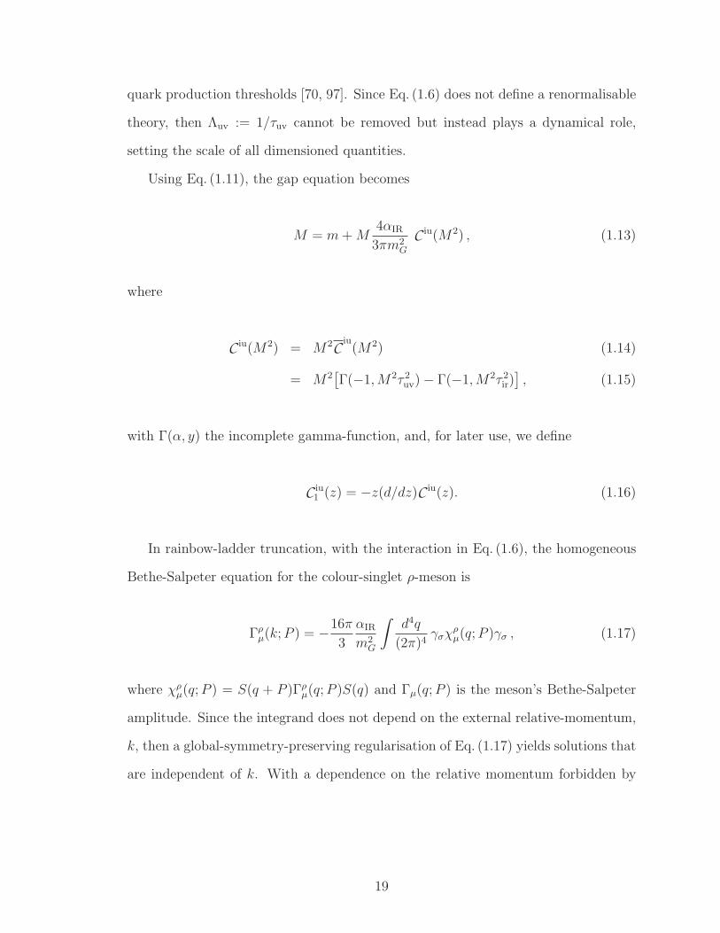
In rainbow-ladder truncation, with the interaction in Eq. (1.6), the homogeneous
Bethe-Salpeter equation for the colour-singlet ρ-meson is
Γρµ(k;P ) = −16π
3
αIR
m2G
∫
d4q
(2π)4γσχ
ρµ(q;P )γσ , (1.17)
where χρµ(q;P ) = S(q + P )Γρ
µ(q;P )S(q) and Γµ(q;P ) is the meson’s Bethe-Salpeter
amplitude. Since the integrand does not depend on the external relative-momentum,
k, then a global-symmetry-preserving regularisation of Eq. (1.17) yields solutions that
are independent of k. With a dependence on the relative momentum forbidden by
19
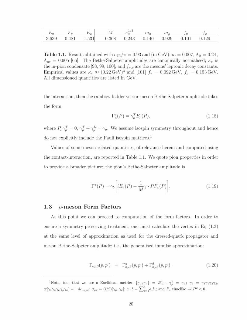
Eπ Fπ Eρ M κ1/3π mπ mρ fπ fρ
3.639 0.481 1.531 0.368 0.243 0.140 0.929 0.101 0.129
Table 1.1. Results obtained with αIR/π = 0.93 and (in GeV): m = 0.007, Λir = 0.24 ,Λuv = 0.905 [66]. The Bethe-Salpeter amplitudes are canonically normalised; κπ isthe in-pion condensate [98, 99, 100]; and fπ,ρ are the mesons’ leptonic decay constants.Empirical values are κπ ≈ (0.22 GeV)3 and [101] fπ = 0.092 GeV, fρ = 0.153 GeV.All dimensioned quantities are listed in GeV.
the interaction, then the rainbow-ladder vector-meson Bethe-Salpeter amplitude takes
the form
Γρµ(P ) = γT
µEρ(P ), (1.18)
where PµγTµ = 0, γT
µ + γLµ = γµ. We assume isospin symmetry throughout and hence
do not explicitly include the Pauli isospin matrices.1
Values of some meson-related quantities, of relevance herein and computed using
the contact-interaction, are reported in Table 1.1. We quote pion properties in order
to provide a broader picture: the pion’s Bethe-Salpeter amplitude is
Γπ(P ) = γ5
[
iEπ(P ) +1
Mγ · PFπ(P )
]
. (1.19)
1.3 ρ-meson Form Factors
At this point we can proceed to computation of the form factors. In order to
ensure a symmetry-preserving treatment, one must calculate the vertex in Eq. (1.3)
at the same level of approximation as used for the dressed-quark propagator and
meson Bethe-Salpeter amplitude; i.e., the generalised impulse approximation:
Γαµβ(p, p′) = Γuαµβ(p, p′) + Γd
αµβ(p, p′) , (1.20)
1Note, too, that we use a Euclidean metric: γµ, γν = 2δµν ; ㆵ = γµ; γ5 = γ4γ1γ2γ3,
tr[γ5γµγνγργσ] = −4ǫµνρσ; σµν = (i/2)[γµ, γν ]; a · b =∑4
i=1aibi; and Pµ timelike ⇒ P 2 < 0.
20
p p′
q
k−+ k++
k−−
Γα Γβ
Γµ
Figure 1.1. Impulse approximation to the ρ-γ vertex, Eq. (1.21): solid lines –dressed-quark propagators; and shaded circles, clockwise from top – Bethe-Salpetervertex for quark-photon coupling, and Bethe-Salpeter amplitudes for the ρ+-meson.
Γfαµβ(p, p′) = 2
∫
d4k
(2π)4TrCD
iΓρj
β (k;−p′)S(k++)
×iΓfµ(k−+, k++)S(k−+)iΓρj
α (k − q/2; p)S(k−−)
, (1.21)
wherein the trace is over colour and spinor indices and kαβ = k + αq/2 + βp/2. We
illustrate Eq. (1.21) in Fig. 1.1.
In evaluating Eq. (1.20) we write:
Sf = S + δCP Sf , f = u, d, (1.22)
where S is given in Eq. (1.9), with the dressed-mass obtained from Eq. (1.10), and the
broken-CP corrections δCP Sf are detailed below; and the ρ-amplitude
Γρjα = γT
αEρ(P ) + ΓρjCPα , (1.23)
with Eρ(P ) explained in connection with Eq. (1.18) and the broken-CP corrections
ΓρjCPα explained below. Our computed values for the dressed-quark mass, M , and Eρ
are listed in Table 1.1.
21

The remaining element in Eq. (1.20) is the dressed-quark–photon vertex. We are
only interested in the q2 = 0 values of the form factors and hence may use
eΓµ(p1, p2) = eQ γµ + iDγ5σµν(p2 − p1)ν (1.24)
=: e diag[euΓuµ(p1, p2),−edΓ
dµ(p1, p2)], (1.25)
where e is the positron charge, Q = diag[eu = 2/3,−ed = 1/3] and D = diag[du,−dd],
with df the EDM of a current quark with flavour f . N.B. The second term in Eq. (1.24)
describes the explicit current-quark EDM interaction in Eq. (1.2). In Sec. 1.4 we show
that the other terms in Eq. (1.2) generate additional contributions that interfere with
this explicit term.
Note that both structures in the vertex, Eq. (1.24), are in general multiplied by
momentum-dependent scalar functions. Naturally, the vector Ward-Takahashi iden-
tity ensures that the coefficient of the Q γµ term is “1” at q2 = 0. In connection with
the tensor term, one knows from Ref. [66] that a tensor vertex is not dressed in the
rainbow-ladder treatment of the contact interaction. However, with a more sophisti-
cated interaction, strong interaction dressing of the γ5σµν part of the quark-photon
vertex might be significant, given that the dressed-quark-photon vertex certainly pos-
sesses a large dressed-quark anomalous magnetic moment term owing to dynamical
chiral symmetry breaking [102]. At q2 = 0, this could enhance the strength of the D
term by as much as a factor of ten. If so, then sensitivity to current-quark EDMs is
greatly magnified. It is worth bearing this in mind.
Working with Eq. (1.3), it is sufficient herein to employ three projection operators:
P 1αµβ = P T
ασ(p)PµP Tσβ(p′) , (1.26a)
P 2αµβ = P T
αα′(p) P Tβ′β(p′)
(
δµβ′qα′ − δµα′qβ′
q2+Pµδα′β′
6p2
)
, (1.26b)
P 3αµβ =
1
2iq2P T
αα′(p)εα′β′µσqσP Tβ′β(p′) , (1.26c)
22
with p′ = p+ q, P = p+ p′, for then
E(0) = limq2→0
1
12m2ρ
P 1αµβΓαµβ , (1.27a)
M (0) = limq2→0
1
4P 2
αµβΓαµβ , (1.27b)
D(0) = limq2→0
P 3αµβΓαµβ , (1.27c)
and µρ = M (0) e/[2mρ], dρ = D(0) e/[2mρ]. So long as a global-symmetry-preserving
regularisation scheme is implemented, E(0) = 1; the value of M (0) is then a predic-
tion, which can both be compared with that produced by other authors and serve as
a benchmark for our prediction of D(0).
At this point one has sufficient information to calculate the ρ-meson’s magnetic
moment. We simplify the denominator in Eq. (1.20) via a Feynman parametrisation:
(
k2++ +M2
)−1 (k2−+ +M2
)−1 (k2−− +M2
)−1
= 2
∫ 1
0
∫ 1−x
0
dx dy
[
k2 +M2 +1
4
[
p2 − 2 (1 − 2x− 2y) p · q + q2]
−(1 − 2y) q · k + (1 − 2x) p · k]−3
. (1.28)
This appears as part of an expression that is integrated over four-dimensional k-
space. The expression is simplified by a shift in integration variables, which exposes
a denominator of the form 1/[k2 + M2]3, with
M2 = M2 + x(x− 1)m2ρ + y(1 − x− y)Q2 . (1.29)
One thereby arrives at a compound expression that involves one-dimensional inte-
grals of the form in Eq. (1.10), which we regularise via Eq. (1.11) and generalisations
thereof; viz.,
23
0 50 100 150 200
2.00
2.05
2.10
2.15
m HMeVL
MH0L
Figure 1.2. Evolution of ρ-meson magnetic moment with current-quark mass. m =170 MeV corresponds to the mass of the s-quark in our treatment of the contactinteraction [69], so the difference between Mρ(0) and Mφ(0) is just 1%.
∫
dss
[s+ ω]2= − d
dωC iu(ω) =: C
iu
1 (ω) , (1.30a)
∫
dss
[s+ ω]3=
1
2
d2
dω2C iu(ω) =: C
iu
2 (ω) , (1.30b)
∫
dss2
[s+ ω]3= C
iu
1 (ω) − ωCiu
2 (ω) , (1.30c)
etc. Details for this component of our computation may be found in Ref. [66] and
pursuing it to completion one obtains the magnetic moment listed in Table 1.2.
We depict the evolution of M (0) with current-quark mass in Fig. 1.2: M (0) is
almost independent of m. This outcome matches that obtained in Ref. [81] using a
renormalisation-group-improved one-gluon exchange kernel and hence a momentum-
dependent dressed-quark mass-function of the type possessed by QCD [103, 104, 105,
106]. The behaviour in Fig. 1.2 will serve to benchmark that of the ρ-meson’s EDM.
1.4 ρ-meson EDM: Formulae
We now turn to computation of the effect of the interaction terms in Eq. (1.2) on
the ρ-meson. There are three types of contribution, which arise separately through
modification of: (1) the quark-photon vertex, Eq. (1.24); (2) the ρ-meson Bethe-
Salpeter amplitude, Eq. (1.23); and (3) the dressed-quark propagator, Eq. (1.22).
24

q
ℓ
µ
P
ℓ
α
ℓ
Figure 1.3. Top – Correction to the quark-photon vertex generated by the four-fermion operator in Eq. (1.31). The unmodified quark-photon vertex is the left dot,whereas the right dot locates insertion of L6. If the internal line represents a circu-lating d-quark then, owing to the L6 insertion, the external lines are u-quarks, andvice versa. Middle – Analogous correction to the ρ-meson Bethe-Salpeter amplitude.The unmodified amplitude is the left dot, whereas the right dot locates insertion ofL6. The lower internal line is an incoming d-quark and the upper external line is anoutgoing u-quark. Bottom – L6-correction to the dressed-quark propagator, with thedot locating the operator insertion. If the outer line is a u-quark, then the internalline is a d-quark; and vice versa.
1.4.1 Four-fermion interaction
We begin with the dimension-six operator, which can be written explicitly as
L6 = iK
2Λ2
[
uadadbγ5ub + uaγ5d
adbub − dadaubγ5ub − daγ5d
aubub]
, (1.31)
with summation over the repeated colour indices. This operator generates all three
types of modification.
25
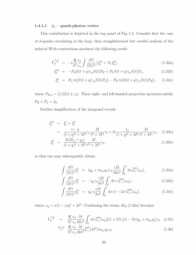
1.4.1.1 L6 – quark-photon vertex
This contribution is depicted in the top panel of Fig. 1.3. Consider first the case
of d-quarks circulating in the loop, then straightforward but careful analysis of the
induced Wick contractions produces the following result:
Γγ
Ld6
µ = −iK
Λ2
ed
eu
∫
d4ℓ
(2π)4
[
I 12µ +NcI
3µ
]
, (1.32a)
I 12µ = −PRS(ℓ+ q)γµS(ℓ)PR + PLS(ℓ+ q)γµS(ℓ)PL , (1.32b)
I 3µ = PL trS(ℓ+ q)γµS(ℓ)PL − PR trS(ℓ+ q)γµS(ℓ)PR , (1.32c)
where PR,L = (1/2)(1±γ5). These right- and left-handed projection operators satisfy
PR + PL = ID.
Further simplification of the integrand reveals
I 12µ = I 1
µ + I 2µ
=iγ · q
(ℓ+ q)2 +M2γµ
M
ℓ2 +M2γ5 + 2i
ℓµ(ℓ+ q)2 +M2
M
ℓ2 +M2γ5 , (1.33a)
I 3µ =
2i(2ℓµ + qµ)
(ℓ+ q)2 +M2
M
ℓ2 +M2γ5 , (1.33b)
so that one may subsequently obtain
∫
d4ℓ
(2π)4I 1µ = (qµ + iσµνqν)γ5
iM
16π2
∫ 1
0
dxCiu
1 (ωq) , (1.34a)
∫
d4ℓ
(2π)4I 2µ = −qµγ5
iM
8π2
∫ 1
0
dx xCiu
1 (ωq) , (1.34b)
∫
d4ℓ
(2π)4I 3µ = qµγ5
iM
8π2
∫ 1
0
dx (1 − 2x) Ciu
1 (ωq) , (1.34c)
where ωq = x(1 − x)q2 +M2. Combining the terms, Eq. (1.32a) becomes
Γγ
Ld6
µ =K
Λ2
ed
eu
M
16π2
∫ 1
0
dxCiu
1 (ωq)[(1 + 2Nc)(1 − 2x)qµ + iσµνqν ]γ5 (1.35)
q2=0=
K
Λ2
ed
eu
M
16π2C
iu
1 (M2)iσµνqνγ5 . (1.36)
26
In the other case, with a u-quark circulating in the loop, one obtains
ΓγLu
6µ
q2=0=
K
Λ2
eu
ed
M
16π2C
iu
1 (M2)iσµνqνγ5 . (1.37)
Plainly, the net correction to the quark-photon vertex can now be cast in the form
of the second term in Eq. (1.24) and hence is readily expressed in D(0).
1.4.1.2 L6 – Bethe-Salpeter amplitude
This correction is depicted in the middle panel of Fig. 1.3. Each of the four terms
in Eq. (1.31) generates a distinct contribution. That from the first and second are:
ΓρL16
α = −iK
Λ2NcEρ PR
×tr
∫
d4ℓ
(2π)4S(ℓ)PRS(ℓ+ P )γT
α , (1.38a)
ΓρL26
α = −iK
Λ2Eρ PR
×∫
d4ℓ
(2π)4S(ℓ+ P )γT
αS(ℓ)PR . (1.38b)
The third and fourth terms are identical, up to sign-change and the replacement
PR → PL; and hence
ΓρL6
α = iK
Λ2Eρ
∫
d4ℓ
(2π)4
[
I 12Tα +NcI
3Tα
]
, (1.39)
where the superscript “T” indicates that γTα is here used in the expressions for I 12,
I 3.
Now, using the formulae of Sec. 1.4.1.1, one arrives at
ΓρL6
α = −iK
Λ2
MEρ
16π2γ5σανPν
∫ 1
0
dxCiu
1 (ωP ) , (1.40)
where ωP = x(1 − x)P 2 +M2, P 2 = −m2ρ. This is one of the additive corrections to
the Bethe-Salpeter amplitude anticipated in Eq. (1.23).
27
1.4.1.3 L6 – quark propagator
The final modification arising from the dimension-six operator is that depicted
in the bottom panel of Fig. 1.3. So long as the correction is small, it modifies the
dressed-quark propagator as follows:
S(k) → S(k) + δL6S(k) = S(k) + S(k)iΓSL6S(k) , (1.41)
where, once again, each of the four terms in Eq. (1.31) contributes. Their sum is
ΓSL6 =K
Λ2
∫
d4ℓ
(2π)4
[
PRS(ℓ)PR − PLS(ℓ)PL
+NcPR trS(ℓ)PR −NcPL trS(ℓ)PL]
. (1.42)
Now
PRS(ℓ)PR − PLS(ℓ)PL =M
ℓ2 +M2γ5
=1
2
[
PR trS(ℓ)PR − PL trS(ℓ)PL]
, (1.43)
so that with little additional algebra one arrives at
δL6S(k) =
i
k2 +M2(1 + 2Nc)
K
Λ2
M
16π2C iu(M2)γ5 . (1.44)
1.4.2 Quark chromo-EDM
The term in the middle line of Eq. (1.2) also generates all three types of modifi-
cation described in the opening lines of this Section. Notably, owing to dynamical
chiral symmetry breaking, the dressed-quark-gluon coupling possesses a chromomag-
netic moment term that, at infrared momenta, is two orders-of-magnitude larger than
the perturbative estimate [102]. One may reasonably expect similar strong-interaction
dressing of a light-quark’s chromo-EDM interaction with a gluon, in which case sen-
sitivity to the current-quark’s chromo-EDM is very much enhanced.
28
+ + q
p+ q/2
p− q/2
q
ℓ− q/2
ℓ+ q/2
p− ℓ
p+ q/2
p− q/2
q
ℓ− q/2
ℓ+ q/2
p− ℓ
p+ q/2
p− q/2
Figure 1.4. Correction to the quark-photon vertex generated by the quark chromo-EDM operator in Eq. (1.2): the incoming and outgoing quark lines have the sameflavour, f . The dot in the left two diagrams locates insertion of LCEDM , whilst thatin the rightmost diagram indicates the second term in Eq. (1.24); i.e., the explicitquark EDM.
1.4.2.1 LCEDM – quark-photon vertex
This contribution is depicted in Fig. 1.4. After a lengthy analysis, in which we
represent the exchanged gluon via Eq. (1.6), the sum of the two leftmost diagrams
produces
Γγ(g)µ =
1
6iπ
dfαIR
m2G
∫ 1
0
dx[
C iu(ωq) − C iu1 (ωq)
]
2qα σµαγ5
−6i[
3(x− 1/2)qµ − pµ
]
γ5
− 1
3π
dfαIR
m2G
∫ 1
0
dxCiu
1 (ωq) ×
6[
ωq − 2M2]
pµγ5 − 6[
(x− 1/2)ωq + 2x(1 − x)q · p]
qµγ5
+M[
((x− 1/2)q + p) · γ]
qασαµγ5
+Mqασαµγ5
[
((x− 1/2)q + p) · γ]
, (1.45)
where, again, df is the chromo-EDM of a quark with flavour f .
As we are interested solely in the EDM, we may consider q2 = 0, at which value
the result simplifies greatly:
Γγ(g)µ =
1
3iπ
dfαIR
m2G
[
C iu(M2) − C iu1 (M2)
][
γ5σµαqα + 3ipµ γ5
]
+1
3π
dfαIR
m2G
Ciu
1 (M2)
[
Mγ · p, γ5σµαqα + 2p · qqµγ5
+6M2pµγ5
]
. (1.46)
29

+P
ℓ− P/2
ℓ+ P/2
p− P/2
p+ P/2
p− ℓ
P
ℓ− P/2
ℓ+ P/2
p− P/2
p+ P/2
p− ℓ
Figure 1.5. Correction to the ρ-meson Bethe-Salpeter amplitude generated by thequark chromo-EDM operator in Eq. (1.2): the incoming line is a d-quark and theoutgoing line is a u-quark. In each case the dot locates insertion of LCEDM .
Plainly, the net correction to the quark-photon vertex from these two diagrams
can now be cast in the form of the second term in Eq. (1.24), which, in fact, is precisely
the rightmost diagram in Fig. 1.4 because q = p2 − p1.
1.4.2.2 LCEDM – Bethe-Salpeter amplitude
This correction is expressed in Fig. 1.5. Owing to similarity between the Leff-
uncorrected ρ-meson amplitude and quark-photon vertex, the results can be read
from those in Sec. 1.4.2.1; viz., with d± = du ± dd,
Γρ(g)α =
1
6iπ
αIR
m2G
Eρ
∫ 1
0
dx[
C iu(ωP ) − C iu1 (ωP )
]
×
[
(d+ − 3(x− 1/2)d−)Pβ − d−pβ
]
σµβγ5P Tµα
+3id+pµγ5P Tµα − 3d−Mγµγ5P T
µα
− 1
3π
αIR
m2G
Eρ
∫ 1
0
dx C iu1 (ωP )
3d+
[
ωP − 2M2]
pµγ5P Tµα
−d−(
[ωP − 2M2][(x− 1/2)Pβ + pβ])
iγ5σβµP Tµα
+Mdd
[
((x− 1/2)P + p) · γ]
Pβσβµγ5P Tµα
+MduPβσβµγ5P Tµα
[
((x− 1/2)P + p) · γ]
. (1.47)
30
+
Figure 1.6. Correction to the dressed-quark propagator generated by the quarkchromo-EDM operator in Eq. (1.2). In each image the dot locates insertion of LCEDM .
In computing the vertex in Eq. (1.20) one must employ Fig. 1.5 and also its charge
conjugate, the form of which is obtained from Eq. (1.47) via the interchange du ↔ dd,
and p→ −p, P → −P .
1.4.2.3 LCEDM – quark propagator
The last modification generated by the chromo-EDM term in Eq. (1.2) is that to
the quark propagator, Fig. 1.6. The self-energy insertion is readily evaluated:
ΓS(g) = df8
π
αIR
m2G
D iu(M2)γ5 , (1.48)
where
D iu(ω) =
∫
dss2
s+ ω→∫ τ2
ir
τ2uv
dτ2
τ 3exp(−τω), (1.49)
so that, with f = u, d,
δ(g)Sf (k) =i
k2 +M2df
8
π
αIR
m2G
D iu(M2)γ5 . (1.50)
1.4.3 θ-term
Owing to a connection between the Higgs mechanism for generating current-quark
masses in the SM and CP violation in the weak interaction, the effect of the θ-term
can completely be expressed through a UA(1) rotation of the current-quark mass-
matrix. We consider the s-quark to be massive and mu = md, in which case the effect
31
of the first term in Eq. (1.2) is expressed simply in a modification of the dressed-quark
propagator:
S(k) → 1
iγ · k +M + i2m θ γ5
(1.51)
mθ small≈ S(k) − 1
k2 +M2
i
2m θ γ5 . (1.52)
1.4.3.1 Dressed-quark anomalous chromomagnetic moment
In our global-symmetry-preserving rainbow-ladder treatment of the contact in-
teraction, the general form of the ρ-meson’s Bethe-Salpeter amplitude is given in
Eq. (1.18). The absence of a term σµνPνFρ(P ) is an artefact of the rainbow-ladder
truncation: even using Eq. (1.6), a Bethe-Salpeter amplitude with Fρ(P ) 6= 0 is ob-
tained in any symmetry-preserving truncation that goes beyond this leading order
[77]. One material consequence of this omission is complete cancellation of all terms
at leading-order in θ, so that the θ-term’s contribution to the ρ-meson’s EDM is
anomalously suppressed in rainbow-ladder truncation. This defect may be amelio-
rated by acknowledging that the dressed-quark-gluon vertex possesses an anomalous
chromomagnetic moment coupling which is enhanced by dynamical chiral symmetry
breaking [102]. We therefore include an effect generated by
Γacmµ (pi, pf ) =
µacm
2Mσµν(pf − pi)ν , (1.53)
where [107] µacm ∼ (−1/4).
In order to explicate the effect we find it convenient to first express collectively the
corrections to the dressed-quark propagator computed above; viz., from Eqs. (1.44),
(1.50), (1.52),
32
S(k) → S(k) − iγ5λ
k2 +M2, (1.54)
λL6= −(1 + 2Nc)
K
Λ2
M
16π2C iu(M2) , (1.55)
λ(g) = −df8
π
αIR
m2G
D iu(M2) , (1.56)
λθ =1
2mθ . (1.57)
Our corrections are now obtained via the diagrams in Fig. 1.5, except that here the
dots represent Eq. (1.53), and one simultaneously adds the correction to one and then
the other propagator. In this way, careful but straightforward computation yields
Γλ,acmµ =
αIR
2iπm2G
λ1µacm2 − λ2µacm
1
2M
∫ 1
0
dx[
C iu(ωP ) − C iu1 (ωP )
]
γµγ5
+αIR
6iπm2G
1
M
∫ 1
0
dx C iu1 (ωP )
3µacm− γ · (p+ (x− 1/2)P )
×[(1 − x)λ1 − xλ2]Pµ + i[
(1 − x)λ1 + xλ2)
][
µacm1 γνPασαµ
−µacm2 Pασαµγν
]
(p+ (x− 1/2)P )ν − λ−M[
µacm+ (p+ (x− 1/2)P )βσµβ
+3iµacm− (p+ (x− 1/2)P )µ
]
γ5 , (1.58)
where µacm± = µacm
1 ± µacm2 , and λi, i = 1, 2 represents the quark propagator correc-
tion on each leg with λ± = λ1 ± λ2.
One can now adapt the general expression in Eq. (1.58) to the particular cases of
relevance herein. The first is the ρ-meson Bethe-Salpeter amplitude. Capitalising on
isospin symmetry, which entails µacmu = µacm
d =: µacm, one finds
Γρ acmα =
αIR
2iπm2G
µacmλ−
2MEρ
∫ 1
0
dx[
C iu(ωP ) − C iu1 (ωP )
]
γµPµαγ5
+αIR
3iπm2G
µacm
2MEρ
∫ 1
0
dx C iu1 (ωP )
i[
(1 − x)λ1
+xλ2](
γβPνσνα − Pνσναγβ
)
(p+ (x− 1/2)P )β
−2λ−MPµα(p+ (x− 1/2)P )νσµν
γ5 , (1.59)
33
where “λ” is constructed from the correction specified in one of Eqs. (1.55) – (1.57).
The other case is the quark-photon vertex, for which the correction is found with
λ1 = λ2 = λ, since the quark flavours are identical, and we need only consider q2 = 0:
Γγ acmµ =
αIR
3πm2G
µacmλ
2MC iu
1 (M2)γ5
[
γ · p , σµαqα]
. (1.60)
1.5 ρ-meson EDM: Results
1.5.1 Analysis without Peccei-Quinn symmetry
In order to obtain a result for the ρ-meson’s EDM, dρ, it remains only to sum the
various contributions derived in Sec. 1.4 as they contribute to Eq. (1.20), evaluated
with the parameter values in Table 1.1:
dρ = −2.88 × 10⁻³ µacm eθ/s
+0.785 (du − dd)
+(1.352 + 0.775µacm)e(du − dd)
−(0.091 − 2.396µacm)e(du + dd)
−esK
Λ2(2.696 − 6.798µacm) × 10−3 . (1.61)
In this formula, df , df carry a dimension of inverse-mass and s = 1 GeV.
A nugatory transformation allows one to rewrite Eq. (1.61) in terms of dimension-
less electric and chromoelectric quark dipole moments; viz.,
dρ = −2.88 × 10⁻³ µacm eθ/s
+vH
Λ2
[
0.785 (Du −Dd)
+(1.352 + 0.775µacm)e(Du − Dd)
−(0.091 − 2.396µacm)e(Du + Dd)
−(1.096 − 2.763µacm) × 10−5 eK
]
, (1.62)
34
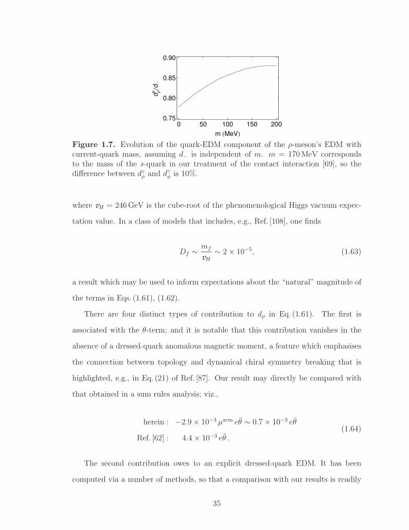
0 50 100 150 2000.75
0.80
0.85
0.90
m HMeVL
dΡΓd-
Figure 1.7. Evolution of the quark-EDM component of the ρ-meson’s EDM withcurrent-quark mass, assuming d− is independent of m. m = 170 MeV correspondsto the mass of the s-quark in our treatment of the contact interaction [69], so thedifference between dγ
ρ and dγφ is 10%.
where vH = 246 GeV is the cube-root of the phenomenological Higgs vacuum expec-
tation value. In a class of models that includes, e.g., Ref. [108], one finds
Df ∼ mf
vH
∼ 2 × 10⁻⁵, (1.63)
a result which may be used to inform expectations about the “natural” magnitude of
the terms in Eqs. (1.61), (1.62).
There are four distinct types of contribution to dρ in Eq. (1.61). The first is
associated with the θ-term; and it is notable that this contribution vanishes in the
absence of a dressed-quark anomalous magnetic moment, a feature which emphasises
the connection between topology and dynamical chiral symmetry breaking that is
highlighted, e.g., in Eq. (21) of Ref. [87]. Our result may directly be compared with
that obtained in a sum rules analysis; viz.,
herein : −2.9 × 10⁻³ µacm eθ ∼ 0.7 × 10⁻³ eθ
Ref. [62] : 4.4 × 10⁻³ eθ .(1.64)
The second contribution owes to an explicit dressed-quark EDM. It has been
computed via a number of methods, so that a comparison with our results is readily
35
compiled:
herein DSE [60] BM [60] nrQM [60] sum rules [62]
0.79 0.72 0.83 1.00 0.51 ,(1.65)
where each entry is multiplied by d− = (du − dd); and DSE [60] summarises results
obtained from momentum-dependent DSE input, BM [60] reports a bag-model re-
sult, and nrQM [60] is the non-relativistic constituent-quark value. We depict the
current-quark mass dependence of this contribution in Fig. 1.7. It is notable that the
magnitude of these results matches an existing DSE estimate of the analogous con-
tribution to the neutron’s EDM [109]. Moreover, based on Ref. [110], a perturbative
analysis would yield 2mρdpertρ = 2md−, where m is the current-quark mass. With the
parameter values employed herein, this is dpertρ = 0.014 d−, which is just ∼ 2% of the
order-of-magnitude specified by the values in Eq. (1.65).
The third contribution to dρ is generated by the quark’s chromoelectric dipole
moment. Its subcomponents are detailed in Table 1.3. The net result is comparable in
magnitude and sign with that produced by the quark EDM, Eq. (1.65). In comparison
with a sum rules computation [62], however, our result is an order of magnitude larger,
has the opposite sign and contains a sizeable d+-term. At least the first two of these
marked discrepancies are insensitive to reasonable variations in µacm. It is worth
emphasising here that our calculation has no other variable parameters: the two
specifying our model, listed in Table 1.1, were fixed in prior studies of an array of
meson and baryon observables [64, 65, 67, 66, 68, 69]. This mismatch will receive
further attention in future work.
The four-fermion interaction is responsible for the final contribution in Eq. (1.61).
Its subcomponents are detailed in Table 1.4. As ours is the first estimate of the
contribution from a dimension-six operator to the ρ-meson’s EDM, there is no ready
substantial comparison. On the other hand, the result in Table 1.4 is quickly seen to
be “natural” in size. The dimension-six operator is associated with a coupling K /Λ2,
36
which has mass-dimension “−2”. In order to obtain a quantity with mass-dimension
“−1”, this coupling must be multiplied by another energy scale. We are interested
in an hadronic EDM, so that scale should be typical of hadron physics; e.g., the
dressed-quark mass “M”. Finally, a loop correction is required for the generation of
an EDM, and loops are characterised by a factor 1/(16π2). Putting these quantities
together yields an expectation based on naive dimensional analysis; viz.,
dD=6ρ ∼ e
1
16π2
M
vH
vHK
Λ2∼ 1 × 10⁻⁵ evHK
Λ2, (1.66)
in agreement with the magnitude of the final row in Table 1.4. Comparison with
Eq. (1.63), furthermore, indicates that in our computation the quark-EDM and dimension-
six contributions are naturally related via
dqEDMρ K ∼ dD=6
ρ . (1.67)
1.5.2 Peccei Quinn Symmetry
The leading term in Eq. (1.62) is that associated with θ. Arising from a dimension-
four operator, this contribution is not suppressed by a large beyond-SM mass-scale.
One may furthermore expect that, absent any symmetry to prevent it, a typical non-
SM for CP-violation will produce large corrections to θ. In order to reconcile this
with the remarkably small upper-bound on θ placed by the neutron’s EDM, one must
accept that the initial value of θ is very finely tuned. There is nothing to prevent
this from being simply an accident of Nature. However, some view that possibility as
aesthetically displeasing and prefer to introduce a new dynamical degree of freedom,
the axion, a pseudo-Goldstone boson, whose role is to cancel the effect of θ [35]. It is
notable that there is currently no empirical evidence in favour of the axion’s existence
and the remaining domain of parameter space is small [115].
37
Notwithstanding this, in the context of EDM estimates it is customary to expose
the possible effect of axion physics on the results in Eq. (1.61) or (1.62). Here there is
a complication. If one considers an extension of the SM with a collection of CP-odd
operators that may mix with the θ-term, then the effective potential describing axion
physics at the hadronic scale can plausibly acquire terms that shift its minimum to
a nonzero value of the effective θ-parameter, θinduced [55]. The quark chromoelectric
dipole moment interaction is one such operator. In its case, within a sum rules
calculation [62], the net effect of this mixing is elimination of θ in favour of a modest
enhancement in magnitude of the coefficients of d± in Eq. (1.61), with no change in
sign.
The implications for our study are plain. Allowing an axion-like mechanism to
play a role, then θ disappears from Eqs. (1.61) and (1.62), and any measurement of
an hadron EDM, here that of the ρ-meson, places a little more stringent constraint
on d± in particular but also on d± and K .
This is, perhaps, particularly relevant to K , since the high-scale physics that
generates this operator will typically also produce a complex phase for the quark
masses. Within the low-energy effective theory of Eq. (1.2), this phase will arise
from one-loop contributions to the quark propagator containing one insertion of the
CP-violating four-quark operator and the quark Yukawa interaction. Consequently,
constraints on θ imply a bound on K . On the other hand, with the elimination of θ
via an axion effective potential, the term modulated by K is exposed to independent
constraint [56]. Computing the contribution of the four-quark CP-violating operator
to the axion potential, determining the resulting dependence of θinduced on K , and
deriving the expression corresponding to Eq. (1.62) will be the subject of future work.
38
1.6 Epilogue
Using the leading-order in a global-symmetry-preserving truncation of QCD’s
Dyson-Schwinger equations, we computed the electric dipole moment of the ρ-meson,
dρ, that is generated by the leading dimension-four and -five CP-violating operators
and an example of a dimension-six operator. We employed a momentum-independent
form for the leading-order kernel in the gap- and Bethe-Salpeter equations. This is
known to produce results for low-energy pseudoscalar- and vector-meson observables
that are indistinguishable from those obtained with the most sophisticated interac-
tions available when they are analysed using the same truncation. Since the dipole
moment is a low-energy observable, our predictions should be similarly reliable, in
which case the framework we employ and elucidate can usefully be adapted to the
more challenging task of computing the neutron’s EDM, dn.
We find that the two dimension-five operators; namely, quark-EDM and -chromo-
EDM, characterised by dq and dq, respectively, produce contributions to dρ whose
coefficients are of the same sign and within a factor of two in magnitude. This
contrasts with an extant sum rules evaluation, in which the coefficients of the contri-
butions have the opposite sign and differ by a factor of four in magnitude. Since all
studies agree within a factor of two on the quark-EDM coefficient, the discrepancy
resides with the chromo-EDM contribution. These differences invite further analysis
and guarantee relevance to a DSE evaluation of the impact of dq on the neutron’s
EDM.
Absent a mechanism that suppresses a θ-term in any beyond-Standard-Model
action, the tight constraints on the magnitude of a contribution from this term to
the neutron’s EDM also apply to contributions from a dimension-six four-fermion
operator to this or another hadron’s EDM. Should such a mechanism exist, however,
we find that a dimension-six operator can match the quark-EDM and chromo-EDM
in importance.
39
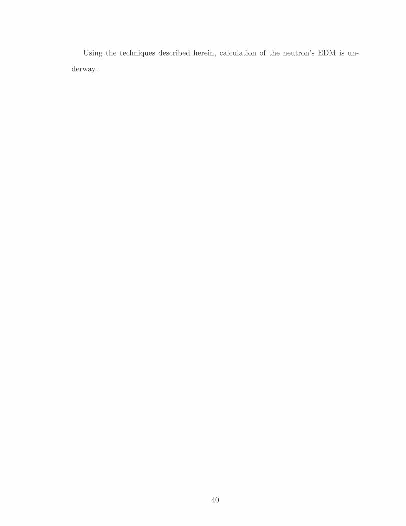
Using the techniques described herein, calculation of the neutron’s EDM is un-
derway.
40
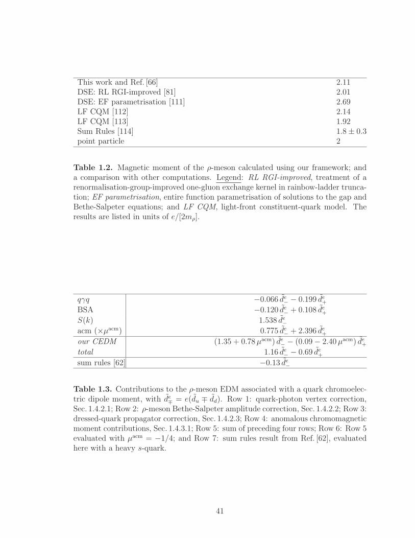
This work and Ref. [66] 2.11DSE: RL RGI-improved [81] 2.01DSE: EF parametrisation [111] 2.69LF CQM [112] 2.14LF CQM [113] 1.92Sum Rules [114] 1.8 ± 0.3point particle 2
Table 1.2. Magnetic moment of the ρ-meson calculated using our framework; anda comparison with other computations. Legend: RL RGI-improved, treatment of arenormalisation-group-improved one-gluon exchange kernel in rainbow-ladder trunca-tion; EF parametrisation, entire function parametrisation of solutions to the gap andBethe-Salpeter equations; and LF CQM, light-front constituent-quark model. Theresults are listed in units of e/[2mρ].
qγq −0.066 de− − 0.199 de
+
BSA −0.120 de− + 0.108 de
+
S(k) 1.538 de−
acm (×µacm) 0.775 de− + 2.396 de
+
our CEDM (1.35 + 0.78µacm) de− − (0.09 − 2.40µacm) de
+
total 1.16 de− − 0.69 de
+
sum rules [62] −0.13 de−
Table 1.3. Contributions to the ρ-meson EDM associated with a quark chromoelec-tric dipole moment, with de
∓ = e(du ∓ dd). Row 1: quark-photon vertex correction,Sec. 1.4.2.1; Row 2: ρ-meson Bethe-Salpeter amplitude correction, Sec. 1.4.2.2; Row 3:dressed-quark propagator correction, Sec. 1.4.2.3; Row 4: anomalous chromomagneticmoment contributions, Sec. 1.4.3.1; Row 5: sum of preceding four rows; Row 6: Row 5evaluated with µacm = −1/4; and Row 7: sum rules result from Ref. [62], evaluatedhere with a heavy s-quark.
41
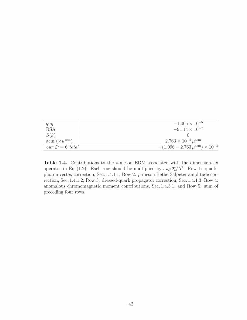
qγq −1.005 × 10⁻⁵
BSA −9.114 × 10⁻⁷
S(k) 0acm (×µacm) 2.763 × 10⁻⁵ µacm
our D = 6 total −(1.096 − 2.763µacm) × 10−5
Table 1.4. Contributions to the ρ-meson EDM associated with the dimension-sixoperator in Eq. (1.2). Each row should be multiplied by evHK /Λ2. Row 1: quark-photon vertex correction, Sec. 1.4.1.1; Row 2: ρ-meson Bethe-Salpeter amplitude cor-rection, Sec. 1.4.1.2; Row 3: dressed-quark propagator correction, Sec. 1.4.1.3; Row 4:anomalous chromomagnetic moment contributions, Sec. 1.4.3.1; and Row 5: sum ofpreceding four rows.
42
CHAPTER 2
SCALAR AND TENSOR CHARGES OF THE NUCLEON
2.1 Introduction
In recent years a global approach to the description of nucleon structure has
emerged, one in which we may express our knowledge of the nucleon in the Wigner
distributions of its basic constituents and thereby provide a multidimensional general-
isation of the familiar parton distribution functions (PDFs). The Wigner distribution
is a quantum mechanics concept analogous to the classical notion of a phase space
distribution. Following from such distributions, a natural interpretation of measured
observables is provided by construction of quantities known as generalised parton dis-
tributions (GPDs) [187, 188, 189, 190, 191, 192, 193, 194] and transverse momentum-
dependent distributions (TMDs) [195, 196, 197, 198, 199, 200, 201]: GPDs are linked
to a spatial tomography of the nucleon; and TMDs allow for its momentum tomog-
raphy. A new generation of experiments aims to provide the empirical information
necessary to develop a phenomenology of nucleon Wigner distributions.
At leading-twist there are eight distinct TMDs, only three of which are nonzero
in the collinear limit; i.e., in the absence of parton transverse momentum within the
target, k⊥ = 0: the unpolarized (f1), helicity (g1L) and transversity (h1T ) distribu-
0Reprinted article with permission from M. Pitschmann, C. Y. Seng, C. D. Roberts andS. M. Schmidt, Phys. Rev. D 91 (2015) 074004, Copyright (2015) by the American Physical So-ciety. DOI: http://dx.doi.org/10.1103/PhysRevD.91.074004
43
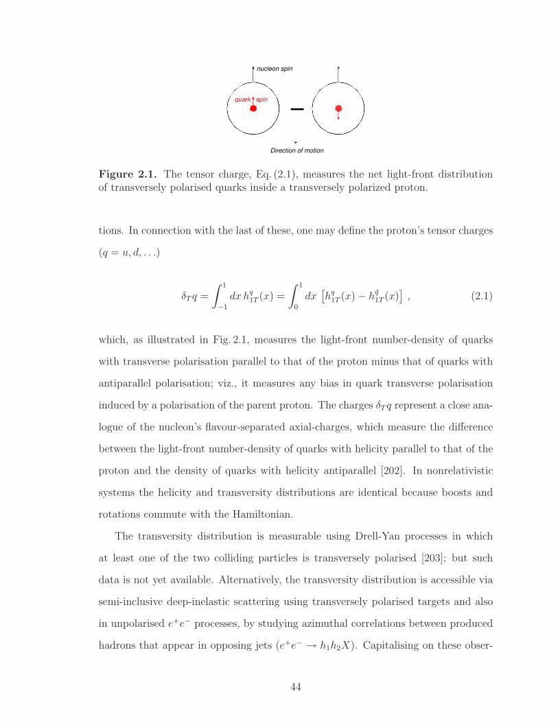
−
Direction of motion
nucleon spin
quark spin
Figure 2.1. The tensor charge, Eq. (2.1), measures the net light-front distributionof transversely polarised quarks inside a transversely polarized proton.
tions. In connection with the last of these, one may define the proton’s tensor charges
(q = u, d, . . .)
δT q =
∫ 1
−1
dx hq1T (x) =
∫ 1
0
dx[
hq1T (x) − hq
1T (x)]
, (2.1)
which, as illustrated in Fig. 2.1, measures the light-front number-density of quarks
with transverse polarisation parallel to that of the proton minus that of quarks with
antiparallel polarisation; viz., it measures any bias in quark transverse polarisation
induced by a polarisation of the parent proton. The charges δT q represent a close ana-
logue of the nucleon’s flavour-separated axial-charges, which measure the difference
between the light-front number-density of quarks with helicity parallel to that of the
proton and the density of quarks with helicity antiparallel [202]. In nonrelativistic
systems the helicity and transversity distributions are identical because boosts and
rotations commute with the Hamiltonian.
The transversity distribution is measurable using Drell-Yan processes in which
at least one of the two colliding particles is transversely polarised [203]; but such
data is not yet available. Alternatively, the transversity distribution is accessible via
semi-inclusive deep-inelastic scattering using transversely polarised targets and also
in unpolarised e+e− processes, by studying azimuthal correlations between produced
hadrons that appear in opposing jets (e+e− → h1h2X). Capitalising on these obser-
44
vations, the transversity distributions were extracted through an analysis of combined
data from the HERMES, COMPASS and Belle collaborations [45]; and those distri-
butions have been used to produce an estimate of the proton’s tensor charges, with
the following flavour-separated results:
δTu = 0.39+0.18−0.12 , δTd = −0.25+0.30
−0.10 , (2.2)
at a renormalisation scale ζA = 0.9 GeV. Given that the tensor charges are a defining
intrinsic property of the nucleon, the magnitude of the errors in Eqs. (2.2) is unsatis-
factory. It is therefore critical to better determine δTu, δTd. Consequently, following
upgrades at the Thomas Jefferson National Accelerator Facility (JLab), it is antici-
pated [204] that experiments [205, 206] in Hall-A (SoLID) and Hall-B (CLAS12) will
provide a far more precise determination of the tensor charges.
Naturally, measurement of the transversity distribution and the tensor charges will
not reveal much about the strong interaction sector of the Standard Model unless these
quantities can be calculated using a framework with a traceable connection to QCD.
This point is emphasised with particular force by the circumstances surrounding the
pion’s valence-quark PDF. As reviewed elsewhere [207], numerous authors suggested
that QCD was challenged by a PDF parametrisation based on a precise πN Drell-Yan
measurement [208]. However, the appearance of nonperturbative calculations within
the framework of continuum QCD [209, 210] forced reanalyses of the cross-section,
with the inclusion of next-to-leading-order evolution [211] and soft-gluon resumma-
tion [212], so that now those claims are known to be false and the pion’s valence-quark
PDF may be viewed as a success for QCD [213]. The comparisons between exper-
iment and computations of the pion and kaon parton distribution amplitudes and
electromagnetic form factors have reached a similar level of understanding [214, 215].
Herein, therefore, we compute the proton tensor charges using a confining, symmetry-
preserving Dyson-Schwinger equation (DSE) treatment of a single quark-quark in-
45
teraction; namely, a vector⊗ vector contact-interaction. This approach has proved
useful in a variety of contexts, which include meson and baryon spectra, and their
electroweak elastic and transition form factors [64, 65, 66, 67, 68, 69, 216, 217, 218,
219, 220]. In fact, so long as the momentum of the probe is smaller in magnitude than
the dressed-quark mass produced by dynamical chiral symmetry breaking (DCSB),
many results obtained in this way are practically indistinguishable from those pro-
duced by the most sophisticated interactions that have thus far been employed in
DSE studies [221, 70, 71, 222].
It is apposite to remark here that confinement and DCSB are two key features of
QCD; and much of the success of the contact-interaction approach owes to its effi-
cacious expression of these emergent phenomena in the Standard Model. They are
explained in some detail elsewhere [221, 70, 71, 222] so that here we remark only that
confinement may be expressed via dynamically-driven changes in the analytic struc-
ture of QCD’s propagators and vertices; and DCSB is the origin of more than 98%
of the mass of visible material in the Universe. These phenomena are intimately con-
nected; and whereas the nature of confinement is still debated, DCSB is a theoretically
established nonperturbative feature of QCD [223], which has widespread, measurable
impacts on hadron observables, e.g. Refs. [69, 217, 224, 225, 226, 227, 228, 215, 229],
so that its expression in QCD is empirically verifiable.
Apart from the hadron physics imperative, the value of the nucleon tensor charges
can be directly related to the visible impact of a dressed-quark electric dipole mo-
ment (EDM) on neutron and proton EDMs [109]. Novel beyond-the-Standard-Model
(BSM) scalar operators may also conceivably be measurable in precision neutron ex-
periments so that one typically considers both the nucleon scalar and tensor charges
when exploring bounds on BSM physics [230]. The sum of the scalar charges of all
active quark flavours is simply the nucleon σ-term, which we therefore also compute
herein.
46
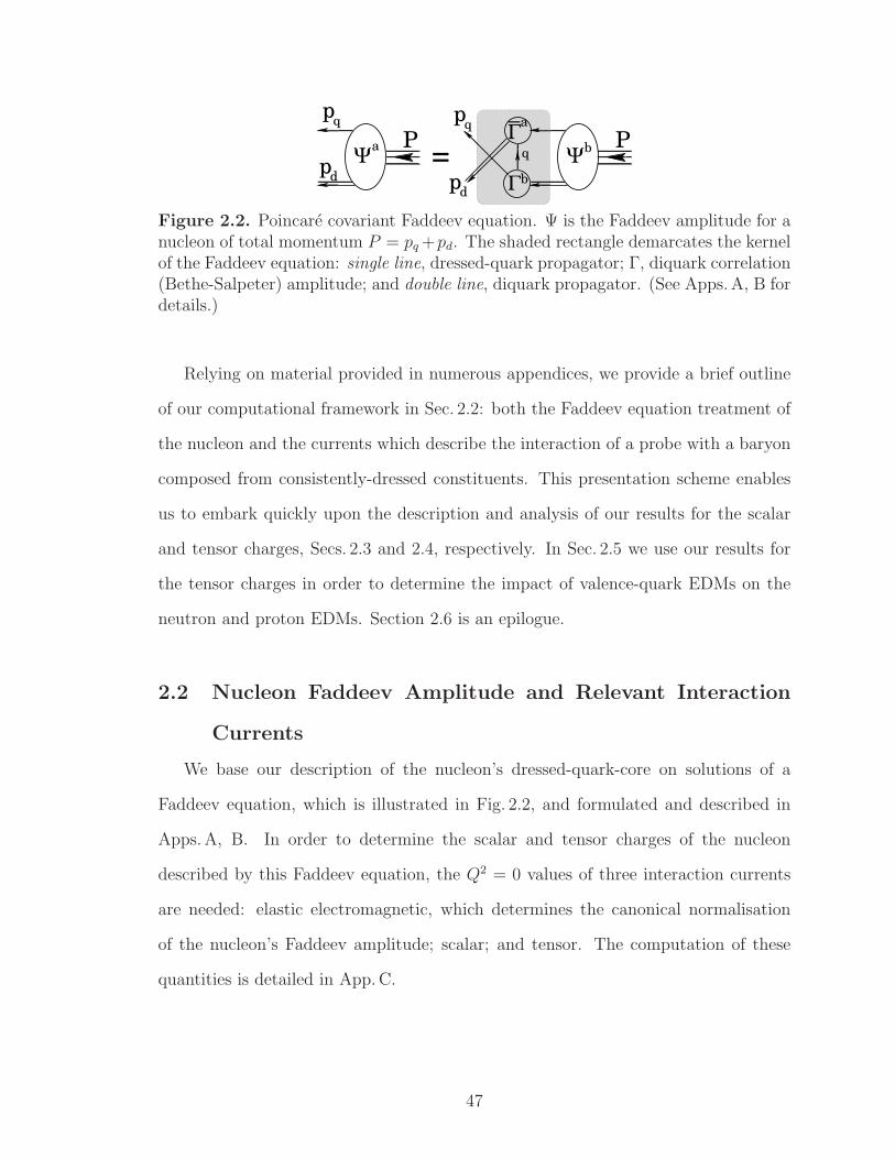
=a
ΨP
pq
pd
Γb
Γ−a
pd
pq
bΨ
Pq
Figure 2.2. Poincare covariant Faddeev equation. Ψ is the Faddeev amplitude for anucleon of total momentum P = pq +pd. The shaded rectangle demarcates the kernelof the Faddeev equation: single line, dressed-quark propagator; Γ, diquark correlation(Bethe-Salpeter) amplitude; and double line, diquark propagator. (See Apps. A, B fordetails.)
Relying on material provided in numerous appendices, we provide a brief outline
of our computational framework in Sec. 2.2: both the Faddeev equation treatment of
the nucleon and the currents which describe the interaction of a probe with a baryon
composed from consistently-dressed constituents. This presentation scheme enables
us to embark quickly upon the description and analysis of our results for the scalar
and tensor charges, Secs. 2.3 and 2.4, respectively. In Sec. 2.5 we use our results for
the tensor charges in order to determine the impact of valence-quark EDMs on the
neutron and proton EDMs. Section 2.6 is an epilogue.
2.2 Nucleon Faddeev Amplitude and Relevant Interaction
Currents
We base our description of the nucleon’s dressed-quark-core on solutions of a
Faddeev equation, which is illustrated in Fig. 2.2, and formulated and described in
Apps. A, B. In order to determine the scalar and tensor charges of the nucleon
described by this Faddeev equation, the Q2 = 0 values of three interaction currents
are needed: elastic electromagnetic, which determines the canonical normalisation
of the nucleon’s Faddeev amplitude; scalar; and tensor. The computation of these
quantities is detailed in App. C.
47
2.3 Sigma-Term
The contribution of a given quark flavour (q = u, d, . . .) to a nucleon’s σ-term is
defined by the matrix element
σq = mq 〈N(p)|qIq|N(p)〉 , (2.3)
where |N(p)〉 is the state vector of a nucleon with four-momentum p. The σ-term is
independent of the renormalisation scale used in the computation, even though the
individual pieces in the product on the right-hand-side (rhs) are not. As explained
in App. E, the scale appropriate to our symmetry-preserving regularisation of the
contact interaction is ζH ≈M , where M is the dressed-quark mass.
Our computed value of the nucleon’s σ-term is reported in Eq. (C.49); viz.,
σN = σu + σd = m 3.05 = 21 MeV. (2.4)
This result is consistent with that obtained using the Feynman-Hellmann theorem
in connection with the results from which Ref. [67] was prepared. An interesting
way to expose this is to recall Eq. (B.28), which states that our analysis describes a
nucleon that is 77% dressed-quark + scalar-diquark and 23% dressed-quark + axial-
vector diquark. In the isospin symmetric limit, which we typically employ, it follows
that
σN = 0.77 [σQ + σqq0 ] + 0.23 [σQ + σqq1 ] (2.5)
= σQ + 0.77σqq0 + 0.23σqq1 , (2.6)
where
48
σQ = m∂M
∂m= 9.6 MeV, (2.7a)
σqq0 = m∂mqq0
∂m= 16 MeV, (2.7b)
σqq1 = m∂mqq1
∂m= 10 MeV, (2.7c)
again computed using material in Ref. [67]. Inserting Eqs. (2.7) into Eq. (2.6), one
obtains σN = 24 MeV.1 Apparently, so far as the contribution of explicit chiral sym-
metry breaking to the mass of the nucleon’s dressed-quark core is concerned, the
contact-interaction nucleon is a simple system. This analysis also shows that our
diagrammatic computational method is sound; and hence Eq. (2.4) is the rainbow-
ladder (RL) truncation2 prediction of a vector⊗ vector contact-interaction treated in
the Faddeev equation via the static approximation. (Inclusion of meson-baryon loop
effects will increase the result in Eq. (2.4) by approximately 15% [231].)
In addition, the fact that Eqs. (2.4) and (2.6) yield similar results emphasises the
important role of diquark correlations because if the nucleon were just a sum of three
massive, weakly-interacting dressed-quarks, then one would have
σ3MN = 3σQ = 29 MeV , (2.8)
which is 21% too large.
Adopting a different perspective, we note that the value in Eq. (2.4) is roughly
one-half that produced by a Faddeev equation kernel that incorporates scalar and
axial-vector diquark correlations in addition to propagators and interaction vertices
that possess QCD-like momentum dependence [231]. It compares similarly with the
1The origin of the 11% mismatch is explained in Sec. C.1.7.
2The rainbow-ladder truncation is the leading-order term in the most widely used, global-symmetry-preserving DSE truncation scheme [76, 77].
49
value inferred in a recent analysis [232] of lattice-QCD results for octet baryon masses
in 2 + 1-flavour QCD:
σN = 45 ± 6 MeV . (2.9)
In order to understand the discrepancy, consider Eqs. (2.7). The value of σQ
matches expectations based on gap equation kernels whose ultraviolet behaviour is
consistent with QCD [231, 233]. On the other hand, with such interactions one
typically finds σqq0 & σqq1 & σρ = 25 MeV. We therefore judge that Eq. (2.4) un-
derestimates the physical value of σN ; and that the mismatch originates primarily
in the rigidity of the diquark Bethe-Salpeter amplitudes produced by the contact in-
teraction, which leads to weaker m-dependence of the diquark (and hence nucleon)
masses than is obtained with more realistic kernels.3 Notwithstanding this, Eq. (2.4)
is a useful benchmark, providing a sensible result via a transparent method.
Further valuable information may be obtained from the results in App. C.2 if
one supposes that the ratio of contact-interaction d- and u-quark contributions is
more reliable than the net value of σN . In this connection, note that for a proton
constituted as a weakly interacting system of three massive dressed-quarks in the
isospin symmetric limitσ3M
N,d
σ3MN,u
=1
2. (2.10)
Comparing this with our computed value
σN,d
σN,u
= 0.65 , (2.11)
one learns that diquark correlations work to accentuate the contribution of the singly-
represented valence-quark to the proton σ-term relative to that of doubly-represented
valence-quarks: the magnification factor is 1.3.
3Consider that if one uses σqq0 = σqq1 = 30MeV, then σN ≈ 40MeV.
50
Let’s take this another step and assume that σN,u, σN,d in App. C.2 respond weakly
to changes in m. This is valid so long as solutions of the dressed-quark gap equation
satisfy
dM
dm
∣
∣
∣
∣
(mu+md)/2
mu,md≪M≈ dM
dm
∣
∣
∣
∣
mu,md
, (2.12)
which is found to be a good approximation in all available studies (see, e.g., Refs. [234,
235]). One may then estimate the effects of isospin symmetry violation owing to the
difference between u- and d-quark current-masses. Taking the value of the mass ratio
from Ref. [181], one finds
mu
md
= 0.48 ± 0.1 ⇒ md σN,d
mu σN,u
= 1.35+0.47−0.30 . (2.13)
Alternatively, one might use the mass ratio inferred from a survey of numerical sim-
ulations of lattice-regularised QCD [236], in which case
mu
md
= 0.47 ± 0.04 ⇒ md σN,d
mu σN,u
= 1.38+0.17−0.14 . (2.14)
We predict, therefore, that the d-quark contribution to that part of the proton’s
mass which arises from explicit chiral symmetry breaking is roughly 37% greater
than that from the u-quark. This value is commensurate with a contemporaneous
estimate based on lattice-QCD [237]. It is noteworthy that if the proton were a
weakly interacting system of three massive dressed-quarks, then Eq. (2.14) would
yield 1.06+0.13−0.11; and hence one finds again that the presence of diquark correlations
within the proton enhances the contribution of d-quarks to the proton’s σ-term.
2.4 Tensor Charge
The tensor charge associated with a given quark flavour in the proton is defined
via the matrix element (q = u, d, . . .)
51
〈P (p, σ)|qσµνq|P (p, σ)〉 = δT q u(p, σ)σµνu(p, σ) , (2.15)
where u(p, σ) is a spinor and |P (p, σ)〉 is a state vector describing a proton with
momentum p and spin σ.4 With δTu, δTd in hand, the isoscalar and isovector tensor
charges are readily computed:
g(0)T = δTu+ δTd , g
(1)T = δTu− δTd . (2.16)
Importantly, the tensor charge is a scale-dependent quantity. Its evolution is discussed
in App. F.
Our analysis of the proton’s tensor charge in a symmetry-preserving RL-truncation
treatment of a vector⊗ vector contact-interaction is detailed in App. C.3. At the
model scale, ζH , which is determined and explained in App. E, we obtain the results
in Table C.3, which represent a parameter-free prediction: the current-quark mass
and the two parameters that define the interaction were fixed elsewhere [66], in a
study of π- and ρ-meson properties.
It is natural to ask for an estimate of the systematic error in the values reported
in Table C.3. As we saw in Sec. 2.3, the error might pessimistically be as much
as a factor of two. However, that is an extreme case because, as observed in the
Introduction, one generally finds that our treatment of the contact interaction pro-
duces results for low-momentum-transfer observables that are practically indistin-
guishable from those produced by RL studies that employ more sophisticated inter-
actions [64, 65, 67, 66, 68, 69, 216, 217, 218, 219, 220]. It is therefore notable that
analyses of hadron physics observables using the RL truncation and one-loop QCD
renormalisation-group-improved (RGI) kernels for the gap and bound-state equations
produce results that are typically within 15% of the experimental value [221]. We
4In the isospin symmetric limit: δpT u := δT u = δn
T d, δpT d := δT d = δn
T u.
52
therefore ascribe a relative error of 15% to the results in Table C.3 so that our pre-
dictions are:
δTu δTd g(0)T g
(1)T
ζH ≈M 0.69(10) −0.14(2) 0.55(8) 0.83(12). (2.17)
One means by which to check our error estimate is to repeat the calculations
described herein using a modern RGI kernel [83] in the gap and bound-state equations.
That has not yet been done but one may nevertheless infer what it might yield.
Consider first Ref. [238], which computes the dressed-quark-tensor vertex using a RL-
treatment of a QCD-based kernel: one observes that the dressed-quark’s tensor charge
is markedly suppressed; namely, with a QCD-based momentum-dependent kernel,
a factor of approximately one-half appears on the rhs of Eq. (C.50). This DCSB-
induced suppression would tend to reduce the values in Eq. (2.17). On the other
hand, the use of a more sophisticated momentum-dependent kernel in the bound-
state equations increases the amount of dressed-quark orbital angular momentum in
the proton, an effect apparent in the reduction of the fraction of proton helicity carried
by dressed u- and d-quarks when one shifts from a contact-interaction framework to
a QCD-kindred approach [226, 229]. Hence, the tensor charges are determined by
two competing effects, the precise balance amongst which can only be revealed by
detailed calculations.
In this context, however, it is worth noting that similar DCSB-induced effects
are observed in connection with gA, the nucleon’s axial charge. The axial-charge
of a dressed-quark is suppressed [202], owing to DCSB; but that is compensated in
the calculation of gA by dressed-quark orbital angular momentum in the nucleon’s
Faddeev wave-function, with the computed value of the nucleon’s axial-charge being
20% larger than that of a dressed-quark. The net effect is that a computation of gA
53
using the framework of Refs. [229] can readily produce a result that is within 15% of
the empirical value [221, 202]. This suggests that our error estimate is reasonable.
The predictions in Eq. (2.17) are quoted at the model scale, whose value is ex-
plained in App. E. In order to make a sensible comparison with estimates obtained
in modern simulations of lattice-regularised QCD, those results must be evolved to
ζ2 = 2 GeV. We therefore list here the results obtained under leading-order evolution
to ζ2 = 2 GeV, obtained via multiplication by the factor in Eq. (F.4):
δTu δTd g(0)T g
(1)T
ζ2 0.55(8) −0.11(2) 0.44(7) 0.66(10). (2.18)
The error in Eq. (F.4) does not propagate significantly into these results.
Notably, the dominant contribution to δTu arises from Diagram 1: tensor probe
interacting with a dressed u-quark with a scalar diquark as the bystander. The tensor
probe interacting with the axial-vector diquark, with a dressed-quark as a spectator,
Diagram 4, produces the next largest piece. However, that is largely cancelled by the
sum of Diagrams 5 and 6: tensor probe causing a transition between scalar- and axial-
vector diquark correlations within the proton whilst the dressed-quark is a bystander.
It is a large negative contribution for both δTu and δTd: indeed, owing to a significant
cancellation between Diagrams 2 and 4 in the d-quark sector, which describe the net
result from quark + axial-vector-diquark contributions, the sum of Diagrams 5 and 6
provides almost the entire result for δTd.
A particularly important result is the impact of the proton’s axial-vector diquark
correlation. As determined in App. C.3.6, with a symmetry-preserving treatment
of a contact interaction, δTd is only nonzero if axial-vector diquark correlations are
present. Significantly, in dynamical calculations the strength of axial-vector diquark
correlations relative to scalar diquark correlations is a measure of DCSB [69]. In the
absence of axial-vector diquark correlations [Eqs. (C.73), Eq. (F.4)]
54
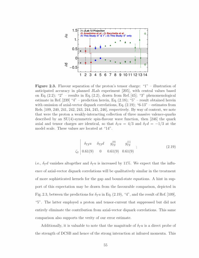
øø
øø
ìì
ìì
ìì
ìì ôô
òò
¨
¨
ææàà
ææ
àà
ò ò
òò
ò
ò
ò
ôô
ôô
ôô
ô
1 2 3 4 5 6 7 8 9 10 11 12 13 14
-0.5
0
0.5
1.
1.5
∆d
∆u
H1L JLab 12 ProjectionH2L Anselmino et al.; H3L Bacchetta et al.H4L This Study: 0+ & 1+; H5L This Study: 0+ only
Figure 2.3. Flavour separation of the proton’s tensor charge: “1” – illustration ofanticipated accuracy in planned JLab experiment [205], with central values basedon Eq. (2.2); “2” – results in Eq. (2.2), drawn from Ref. [45]; “3” phenomenologicalestimate in Ref. [239] “4” – prediction herein, Eq. (2.18); “5” – result obtained hereinwith omission of axial-vector diquark correlations, Eq. (2.19); “6-13” – estimates fromRefs. [109, 240, 241, 242, 243, 244, 245, 246], respectively. By way of context, we notethat were the proton a weakly-interacting collection of three massive valence-quarksdescribed by an SU(4)-symmetric spin-flavour wave function, then [246] the quarkaxial and tensor charges are identical, so that δTu = 4/3 and δTd = −1/3 at themodel scale. These values are located at “14”.
δT6 1u δT6 1d g(0)T6 1 g
(1)T6 1
ζ2 0.61(9) 0 0.61(9) 0.61(9); (2.19)
i.e., δTd vanishes altogether and δTu is increased by 11%. We expect that the influ-
ence of axial-vector diquark correlations will be qualitatively similar in the treatment
of more sophisticated kernels for the gap and bound-state equations. A hint in sup-
port of this expectation may be drawn from the favourable comparison, depicted in
Fig. 2.3, between the predictions for δTu in Eq. (2.19), “4”, and the result of Ref. [109],
“5”. The latter employed a proton and tensor-current that suppressed but did not
entirely eliminate the contribution from axial-vector diquark correlations. This same
comparison also supports the verity of our error estimate.
Additionally, it is valuable to note that the magnitude of δTu is a direct probe of
the strength of DCSB and hence of the strong interaction at infrared momenta. This
55
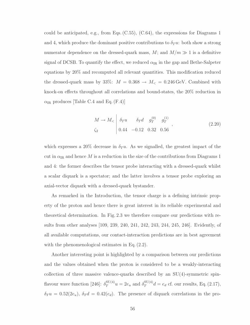
could be anticipated, e.g., from Eqs. (C.55), (C.64), the expressions for Diagrams 1
and 4, which produce the dominant positive contributions to δTu: both show a strong
numerator dependence on the dressed-quark mass, M ; and M/m ≫ 1 is a definitive
signal of DCSB. To quantify the effect, we reduced αIR in the gap and Bethe-Salpeter
equations by 20% and recomputed all relevant quantities. This modification reduced
the dressed-quark mass by 33%: M = 0.368 → M< = 0.246 GeV. Combined with
knock-on effects throughout all correlations and bound-states, the 20% reduction in
αIR produces [Table C.4 and Eq. (F.4)]
M →M< δTu δTd g(0)T g
(1)T
ζ2 0.44 −0.12 0.32 0.56, (2.20)
which expresses a 20% decrease in δTu. As we signalled, the greatest impact of the
cut in αIR and hence M is a reduction in the size of the contributions from Diagrams 1
and 4: the former describes the tensor probe interacting with a dressed-quark whilst
a scalar diquark is a spectator; and the latter involves a tensor probe exploring an
axial-vector diquark with a dressed-quark bystander.
As remarked in the Introduction, the tensor charge is a defining intrinsic prop-
erty of the proton and hence there is great interest in its reliable experimental and
theoretical determination. In Fig. 2.3 we therefore compare our predictions with re-
sults from other analyses [109, 239, 240, 241, 242, 243, 244, 245, 246]. Evidently, of
all available computations, our contact-interaction predictions are in best agreement
with the phenomenological estimates in Eq. (2.2).
Another interesting point is highlighted by a comparison between our predictions
and the values obtained when the proton is considered to be a weakly-interacting
collection of three massive valence-quarks described by an SU(4)-symmetric spin-
flavour wave function [246]: δSU(4)T u = 2eu and δ
SU(4)T d = ed cf. our results, Eq. (2.17),
δTu = 0.52(2eu), δTd = 0.42(ed). The presence of diquark correlations in the pro-
56
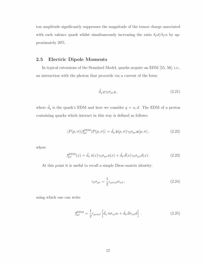
ton amplitude significantly suppresses the magnitude of the tensor charge associated
with each valence quark whilst simultaneously increasing the ratio δTd/δTu by ap-
proximately 20%.
2.5 Electric Dipole Moments
In typical extensions of the Standard Model, quarks acquire an EDM [55, 56]; i.e.,
an interaction with the photon that proceeds via a current of the form:
dq qγ5σµνq , (2.21)
where dq is the quark’s EDM and here we consider q = u, d. The EDM of a proton
containing quarks which interact in this way is defined as follows:
〈P (p, σ)|J EDMµν |P (p, σ)〉 = dp u(p, σ)γ5σµνu(p, σ) , (2.22)
where
J EDMµν (x) = du u(x)γ5σµνu(x) + dd d(x)γ5σµνd(x) . (2.23)
At this point it is useful to recall a simple Dirac-matrix identity:
γ5σµν =1
2εµναβσαβ , (2.24)
using which one can write
J EDMµν =
1
2εµναβ
[
du uσαβu+ dd dσαβd]
. (2.25)
57
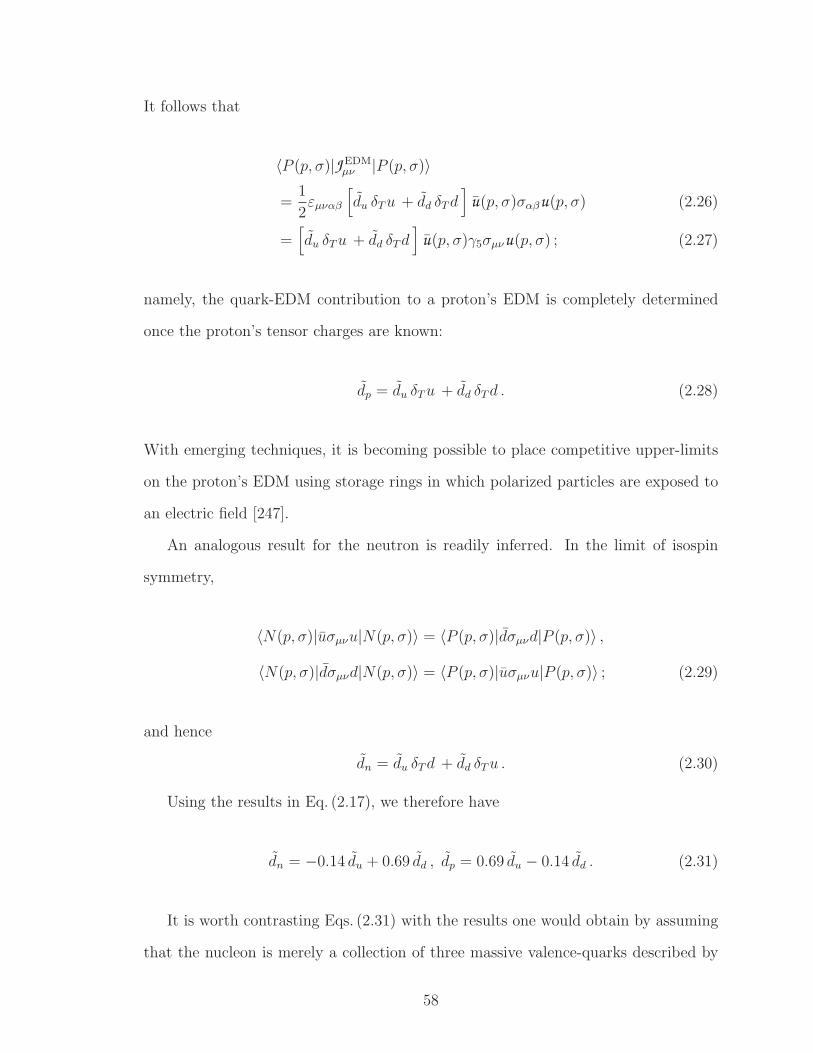
It follows that
〈P (p, σ)|J EDMµν |P (p, σ)〉
=1
2εµναβ
[
du δTu + dd δTd]
u(p, σ)σαβu(p, σ) (2.26)
=[
du δTu + dd δTd]
u(p, σ)γ5σµνu(p, σ) ; (2.27)
namely, the quark-EDM contribution to a proton’s EDM is completely determined
once the proton’s tensor charges are known:
dp = du δTu + dd δTd . (2.28)
With emerging techniques, it is becoming possible to place competitive upper-limits
on the proton’s EDM using storage rings in which polarized particles are exposed to
an electric field [247].
An analogous result for the neutron is readily inferred. In the limit of isospin
symmetry,
〈N(p, σ)|uσµνu|N(p, σ)〉 = 〈P (p, σ)|dσµνd|P (p, σ)〉 ,
〈N(p, σ)|dσµνd|N(p, σ)〉 = 〈P (p, σ)|uσµνu|P (p, σ)〉 ; (2.29)
and hence
dn = du δTd + dd δTu . (2.30)
Using the results in Eq. (2.17), we therefore have
dn = −0.14 du + 0.69 dd , dp = 0.69 du − 0.14 dd . (2.31)
It is worth contrasting Eqs. (2.31) with the results one would obtain by assuming
that the nucleon is merely a collection of three massive valence-quarks described by
58
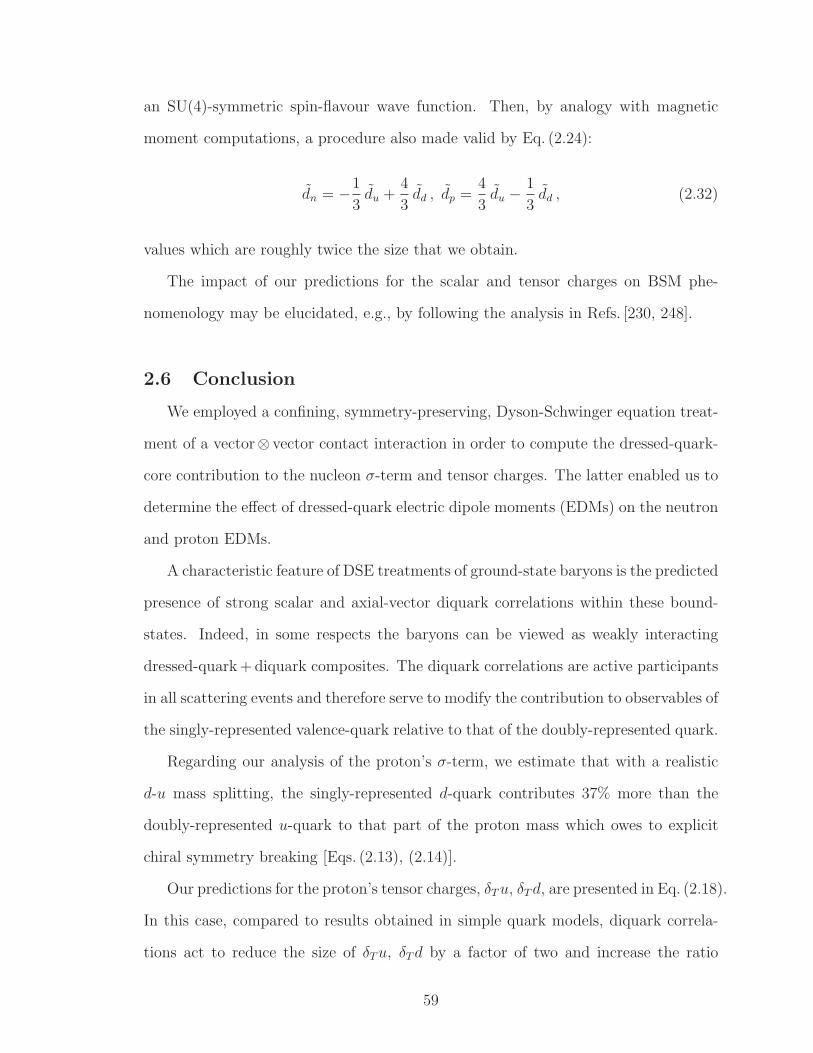
an SU(4)-symmetric spin-flavour wave function. Then, by analogy with magnetic
moment computations, a procedure also made valid by Eq. (2.24):
dn = −1
3du +
4
3dd , dp =
4
3du −
1
3dd , (2.32)
values which are roughly twice the size that we obtain.
The impact of our predictions for the scalar and tensor charges on BSM phe-
nomenology may be elucidated, e.g., by following the analysis in Refs. [230, 248].
2.6 Conclusion
We employed a confining, symmetry-preserving, Dyson-Schwinger equation treat-
ment of a vector⊗ vector contact interaction in order to compute the dressed-quark-
core contribution to the nucleon σ-term and tensor charges. The latter enabled us to
determine the effect of dressed-quark electric dipole moments (EDMs) on the neutron
and proton EDMs.
A characteristic feature of DSE treatments of ground-state baryons is the predicted
presence of strong scalar and axial-vector diquark correlations within these bound-
states. Indeed, in some respects the baryons can be viewed as weakly interacting
dressed-quark + diquark composites. The diquark correlations are active participants
in all scattering events and therefore serve to modify the contribution to observables of
the singly-represented valence-quark relative to that of the doubly-represented quark.
Regarding our analysis of the proton’s σ-term, we estimate that with a realistic
d-u mass splitting, the singly-represented d-quark contributes 37% more than the
doubly-represented u-quark to that part of the proton mass which owes to explicit
chiral symmetry breaking [Eqs. (2.13), (2.14)].
Our predictions for the proton’s tensor charges, δTu, δTd, are presented in Eq. (2.18).
In this case, compared to results obtained in simple quark models, diquark correla-
tions act to reduce the size of δTu, δTd by a factor of two and increase the ratio
59
δTd/δTu by roughly 20%. Two additional observations are particularly significant.
First, the magnitude of δTu is a direct measure of the strength of DCSB in the Stan-
dard Model, diminishing rapidly with the difference between the scales of dynamical
and explicit chiral symmetry breaking. Second, δTd measures the strength of axial-
vector diquark correlations in the proton, vanishing with P1+/P0+ ; i.e., the ratio of
axial-vector- and scalar-diquark interaction probabilities, which is also a measure of
DCSB.
Our analysis of the Faddeev equation employed a simplifying truncation; viz., a
variant of the so-called static approximation. A natural next step is recalculation of
the tensor charges after eliminating that truncation. Subsequently or simultaneously,
one might also employ the approaches of Refs. [249, 229] in order to obtain DSE
predictions with a more direct connection to QCD.
60
CHAPTER 3
AN INTRODUCTION TO THE CHIRAL
PERTURBATION THEORY
In this chapter we provide a brief introduction to the Chiral Perturbation Theory
(ChPT) which is a low-energy effective theory of Quantum Chromodynamics (QCD)
that describes the strong interaction governing interactions between hadrons. There
are many pedagogical articles of this topic and here we mainly follow the logic and
notations in Ref. [172].
3.1 The motivation
QCD is long believed to be the appropriate theory for the strong interaction.
It is an SU(3)c non-Abelian gauge theory that can be described by the following
Lagrangian:
L =∑
q
qiD/ q −mq qq −1
4Ga
µνGaµν (3.1)
where q is the quark field and iDµ ≡ i∂µ − gsTaAa
µ is the SU(3)c covariant derivative.
The free parameters in the theory are the strong coupling constant gs and the quark
masses mq.
As we have explained in the introduction, QCD is perturbative at high energy and
is extremely successful in this regime, examples including the prediction of scaling
violation behavior in deep inelastic scattering (DIS). On the other hand, the theory
becomes highly non-perturbative when the energy scale is lowered to the mass of
light hadrons as the running coupling constant gs(µ) diverges in the infrared limit.
61
Therefore conventional perturbative treatment to QCD is not applicable for the study
of the low-energy properties of hadrons.
Lattice QCD (LQCD) is currently the only promising way to tackle this problem
from the first principle. It involves numerical evaluations of the QCD path integral in
a discretized spacetime using Monte Carlo method. This method is proved to be ex-
tremely successful in many areas, for example the precise reproduction of the hadronic
spectrum. However it applicability is also severely limited by various technical issues
such as the large amount of CPU time. The alternative way to approach is problem
is through the application of effective field theories (EFTs) which are theories that
try to mimic some, if not all, of the properties of QCD in the infrared limit. These
theories are suitably engineered such that calculations in the low energy regime are
tractable.
ChPT is the most general effective field theory at low energy that is constructed
based on one particular symmetry of QCD, namely the chiral symmetry. Instead of
quarks and gluons, the degrees of freedom in ChPT are mesons and baryons. It is
particularly successful in describing the residual strong interaction between hadrons
that involves exchange of light mesons. In this chapter we shall introduce the basic
concepts and ingredients needed for the construction of ChPT Lagrangian without
diving into any specific calculation of Feynman diagrams. These basic concepts are
very helpful for the understanding of most of the contents in the next two chapters.
3.2 Chiral symmetry and spontaneous symmetry breaking
3.2.1 Chiral transformation
Apart from the color SU(3), the QCD Lagrangian possesses another symmetry
known as the chiral symmetry in the limit of massless quarks. To be definite let
us consider the QCD with two lightest quark u and d (the discussion below can
be straightforwardly generalized to include the strange quark). We can separate
62
each quark field into its left- and right-handed components and define the following
doublets:
QL/R ≡
u
d
L/R
. (3.2)
The two-flavor QCD Lagrangian can then be rewritten as
L = QLiDµQL + QRiDµQR − QRMQL − QLM†QR − 1
4Ga
µνGaµν (3.3)
where M = diag(mu md) is the quark mass matrix. It is clear that if we take the
quark masses to be zero then the quark doublet fields with different handedness do
not mix with each other. In other words, the massless two-flavor QCD Lagrangian is
invariant under the following SU(2)L × SU(2)R transformation:
SU(2)L : QL → ULQL
SU(2)R : QR → URQR (3.4)
where UL/R ≡ expi~θL/R·~τ/2 are two independent 2×2 special unitary matrices. This
symmetry is explicitly broken by the quark mass matrix M , however since current
quark masses mu and md are only a few MeV, much lighter than the lightest hadron
mass mπ0 ≈ 135 MeV, so one naively expects the chiral symmetry to be pretty well
respected. It is also extremely useful to realize that the SU(2)L × SU(2)R symmetry
is equivalent to an SU(2)V ×SU(2)A symmetry defined by the following “vector” and
“axial” transformation to the quark doublet:
SU(2)V : Q → expi~θV · ~τ2Q
SU(2)A : Q → expi~θA · ~τ2γ5Q. (3.5)
In particular, the SU(2)V symmetry is known as the isospin symmetry and it is a
good symmetry even with non-zero quark masses provided that mu = md.
63
3.2.2 Spontaneous symmetry breaking
Unlike the isospin symmetry which is proven to be a good approximate symmetry,
nature does not seem to respect the SU(2)A symmetry. A clear evidence is the
following: one can easily prove that if SU(2)A is a good symmetry, then it implies
that for any hadron (made up of light quarks) there must be a corresponding hadron
with the same mass but with the opposite parity. This “parity doubling” effect
is however not observed experimentally. For example, let us consider the lightest
Jp = (1/2)+ baryon (i.e. proton) which has a mass of 938 MeV. If parity doubling
is true, one shall observe a Jp = (1/2)− baryon with approximately the same mass.
Such baryon is however never been observed; the lightest (1/2)− baryon has a mass
around 1535 MeV which can never be interpreted as the parity counterpart of the
proton.
The non-existence of the parity doubling could be explained if the QCD vacuum
|0〉 is non-invariant under the axial transformation, i.e.
QaA |0〉 6= 0 (3.6)
where QaA ≡
∫
d3xQγ0γ5τa
2Q is the conserved charge of SU(2)A. The non-invariance
of the vacuum under a certain symmetry signifies a spontaneous symmetry breaking
(SSB). According to the Nambu-Goldstone theorem, a SSB implies existence of mass-
less spin-zero bosons known as Nambu-Goldstone (NG) bosons. Indeed, we find that
the lightest pseudo-scalar mesons (i.e. the pion triplet) have masses around 135-140
MeV which are much lighter than all the remaining hadrons. We may then identify
them as the NG bosons due to the SSB of the SU(2)A symmetry. Their non-zero
masses are simply due to the existence of small quark masses that explicitly breaks
SU(2)A. Finally we should point out that even though the non-observation of par-
ity doubling and the existence of very light pions are significant evidence that SSB
indeed happens in QCD, but so far there is no rigorous proof that this is indeed the
64
case based on first-principle calculation. ChPT is therefore an effective field theory
of QCD based on the assumption that SSB takes place at low energy and the pion
triplet are the corresponding NG bosons.
3.3 Non-linear realization of NG bosons
In this section we want to introduce the concept of the non-linear representation
of NG bosons which is crucial in the construction of the ChPT Lagrangian.
3.3.1 Basic idea
In order to easily understand the idea let us consider the following simple example.
Imagine a Lagrangian L(φ) which possesses a symmetry group h1 ×h2, and we know
that the symmetry h1 (say with m generators) is spontaneously broken while h2
remains a good symmetry. Then, we may parameterize the field φ(x) as the following:
φ(x) = R (ξ(x))ρ(x) (3.7)
where R is the transformation matrix of h1 and ξ(x) = (ξ1(x), ξ2(x), ...ξm(x)) are
the “rotational angles” of the symmetry transformation h1, except that now they
are spacetime-dependent fields. Finally, ρ(x) is a field which is invariant under the
transformation h1.
With this parameterization it is clear that the fields ξi(x) are automatically the
NG bosons (up to normalization factors) due to the SBB of h1. The way to see this
is very simple: if ξi(x) are spacetime-independent, then we can perform another h1
transformation on φ(x):
φ′(x) = R −1(ξ)φ(x) = R −1(ξ)R (ξ)ρ(x) = ρ(x). (3.8)
Now, since L is invariant under h1, so we will have L(φ) = L(φ′) = L(ρ), i.e. the
fields ξi will not appear in the Lagrangian. This implies that, if the fields ξi are
65
to appear in the Lagrangian then they must be spacetime-dependent. The only way
for this to happen is that every term in the Lagrangian L which involve only ξi
must also involve derivatives on ξi. This immediately excludes any mass term of
ξi as it does not involve derivatives. They are therefore massless bosons and can
be identified as NG bosons due to the SSB of the symmetry group h1.
3.3.2 Example of non-linear realization: SU(2)L × SU(2)R
To elaborate the general idea above and derive one essential building block for
the actual ChPT, let us proceed to the study of non-linear realization of Goldstone
bosons in a simple theory with spontaneously-broken SU(2)L × SU(2)R symmetry.
The fermionic building blocks can be written as ψR and ψL which transform as ψR →
URψR and ψL → ULψL under SU(2)L × SU(2)R. Now, if we want to write down an
SU(2)L×SU(2)R-invariant theory that involves interaction between ψR and ψL, then
it is essential to introduce a 2 × 2 matrix Σ(x) that transforms as:
Σ(x) → URΣ(x)U †L. (3.9)
With this matrix, terms like ψRΣψL will be invariant.
Recall from the previous section that SU(2)R × SU(2)L is also equivalent to
SU(2)V × SU(2)A. Starting from Eq. (3.9), it is easy to show that Σ(x) should
transform under SU(2)A as
SU(2)A : Σ(x) → expi~θA · ~τ2Σ(x) expi~θA · ~τ
2 (3.10)
where ~θA ≡ (~θR − ~θL)/2. Now, assuming that SU(2)A is spontaneously broken, we
may follow the spirit of non-linear realization introduced in the previous subsection
and reparameterize Σ(x) as
Σ(x) ≡√
U(x)σ(x)√
U(x) (3.11)
66
where√
U(x) ≡ expi~ξ(x) · ~τ2 (3.12)
and the field σ(x) is invariant under SU(2)A. By construction, the triplet field ~ξ(x)
plays the role of NG bosons (up to normalization factors). Furthermore, we require
that ~ξ(x) transforms as a triplet under the good symmetry SU(2)V just like what
happens to ordinary pions. One may show that this requirement implies the following
transformation rule of√
U(x) under SU(2)V :
SU(2)V :√
U(x) → expi~θV · ~τ2√
U(x) exp−i~θV · ~τ2 (3.13)
(~θV ≡ (~θR +~θL)/2). Combining Eq. (3.10) and (3.13) we immediately see that σ(x) is
an invariant under SU(2)V ×SU(2)A. It is therefore a scalar field instead of a matrix.
Finally, the Σ(x) matrix can now be written as
Σ(x) = σ(x)U(x) (3.14)
where U(x) = expi~τ · ~ξ(x) and transforms under SU(2)L × SU(2)R as U(x) →
URU(x)U †L. The scalar field σ(x) is a massive excitation and it plays no role in
maintaining the symmetry of the Lagrangian, therefore it can be integrated out in
the effective theory. On the other hand, the matrix U(x) serves as the non-linear
realization of the NG bosons and will be one of the main building blocks of our
low-energy effective theory of QCD.
3.4 ChPT for NG bosons
Now we are ready to construct the effective field theory of QCD based on symmetry
consideration. As we showed in Sec. 3.2, the two-flavor QCD possesses the following
properties:
1. It is invariant under SU(2)V × SU(2)A in the massless quark limit;
67
2. SU(2)A is spontaneously broken at low energy and pions are the NG bosons;
3. SU(2)A is explicitly broken by the insertion of quark mass matrix M .
It is then natural to require our effective theory to obey the properties listed above. In
fact, we want to construct the MOST GENERAL Lagrangian that satisfies these three
requirements. Obviously there are infinitely many terms with arbitrary mass dimen-
sions that may satisfy these three criteria and we shall include all of them in our La-
grangian. This unavoidably makes ChPT an unrenormalizable theory which is a com-
mon feature for most of the effective field theories. Despite its non-renormalizability,
ChPT still possesses finite predictive power due to the following reason. Due to the
non-linear realization, terms involving pions must contain either derivatives or inser-
tions of quark mass matrix M (and we will see later that m2π ∼ mq). It therefore
exists a “power counting” rule saying that one may arrange terms in ChPT according
to an increasing power of p/Λχ where p is either the pion mass or a small momentum
of pion while Λχ ∼1 GeV is an energy scale related to the chiral symmetry breaking.
Hence, for any given precision level, one only needs to include a finite number of terms
in the chiral Lagrangian as the remaining terms are suppressed by more powers of
p/Λχ. This concept of power counting is essential as it makes calculations in ChPT
tractable.
3.4.1 O(p2): Chiral invariant terms
Let us concentrate on the pure Goldstone terms in ChPT in this section. These
terms can be constructed using the matrix U(x) we discussed in the previous section.
Following standard notations, we define the normalized pion fields ~π(x) through
U(x) = expi~π(x) · ~τFπ
(3.15)
and the parameter Fπ is known as the pion decay constant. In our convention Fπ ≈ 93
MeV but it is also worth knowing that in other conventions Fπ may take different
68
values (the most common example is that Fπ ≈ 186 MeV in the SO(4) representation
of ChPT).
We start by constructing the leading order chiral-invariant Lagrangian using U(x).
As discussed in Sec. 3.3, any chiral-invariant term of pions must involve derivatives.
One may easily show that the only chiral-invariant operator in O(p2) is given by:
L (2)inv =
F 2π
4Tr[(∂µU)(∂µU †)]. (3.16)
The prefactor F 2π/4 serves for the normalization of the pion kinetic term. Expansion
of this Lagrangian according to power of pion fields gives:
L (2)inv =
1
2(∂µ~π)2 +
1
6F 2π
[(~π · ∂µ~π)2 − ~π2(∂µ~π)2] +O(π6) (3.17)
which gives the pion kinetic terms as well as interaction terms involving even number
of pions. The interaction strengths of different terms are all inter-related due to chiral
symmetry.
3.4.2 Spurion and chiral symmetry breaking terms at O(p2)
Eq. (3.16) is not the only available term at O(p2) because we need also to include
chiral symmetry breaking terms at the same order. These terms involve insertions
of quark mass matrix M following definite rules. Before we proceed, it is useful to
introduce the concept of “spurion” which is crucial in constructions of symmetry-
breaking terms in an effective theory. To understand this concept let us consider the
quark mass term in QCD. It has the following form:
LmQCD = −QRMQL + h.c.. (3.18)
This term is obviously not chiral invariant, however it “would be” chiral invariant
if we imagine that the constant matrix M would transform as M → URMU †L under
69
SU(2)L × SU(2)R. The matrix M is an example of spurion which is defined as a
constant quantity which would make a given theory invariant under certain transfor-
mation if we imagine that it would transform according to some specific rule.
Since ChPT is an effective theory of QCD it should break chiral symmetry explic-
itly in the exact same ways as QCD does, namely: one should construct operators
involving insertions of the constant quark mass matrix M in such as way that, if
M → URMU †L under chiral rotation then these operators would be chiral invariant.
There is only one such operator at leading order, namely:
L (2)m =
F 2πB0
2Tr[MU † + UM †]. (3.19)
Here B0 is a free parameter with mass dimension 1. The expansion of L (2)m gives:
L (2)m = F 2
πB0(mu +md)(1 − ~π2
2! · F 2π
+(~π2)2
4! · F 4π
) +O(π6). (3.20)
We obtain from L (2)m a constant term, an isospin-invariant pion mass term and a
series of interaction terms with even number of pions. The squared pion mass is then
identified as m2π = B0(mu +md). It is interesting to notice that mπ ∼ √
mq, i.e. the
pion mass depends non-analytically to the quark masses.
Finally, combining Eq. (3.16) and (3.19) we obtain the full mesonic chiral La-
grangian at O(p2):
L (2) =F 2
π
4Tr[(∂µU)(∂µU †)] +
F 2πB0
2Tr[MU † + UM †]
= const +1
2(∂µ~π)2 − m2
π
2~π2 +
1
6F 2π
[(~π · ∂µ~π)2 − ~π2(∂µ~π)2] +m2
π
24F 2π
(~π2)2
+O(π6) (3.21)
3.4.3 Brief discussion of O(p4) Lagrangian
If we restrict our requirement of precision level to O(p2), then what we need is the
application of Eq. (3.21) at tree-level. However, to increase our precision to O(p4)
70
one needs to include extra terms in the chiral Lagrangian at this order. If we ignore
the coupling with external fields then the relevant terms are:
L (4) = L1Tr[(∂µU)(∂µU †)]2 + L2Tr[(∂µU)(∂νU†)]Tr[(∂µU)(∂νU †)]
+L3Tr[(∂µU)(∂µU †)(∂νU)(∂νU †)] + L4Tr[(∂µU)(∂µU †)]Tr[MU † + UM †]
+L5Tr[(∂µU)(∂µU †)(MU † + UM †)] + L6Tr[MU † + UM †]2
+L7Tr[MU † − UM †]2 + L8Tr[MU †MU † + UM †UM †]. (3.22)
The parameter Li are low energy constants (LECs) which cannot be determined
by any symmetry argument.
To obtain full results up to O(p4) one needs to apply Eq. (3.21) to one loop as
well as Eq. (3.22) at tree level. In general the 1-loop integrals contributed by the
O(p2) Lagrangian contain UV-divergences and these divergences can be canceled by
the O(p4) low energy constants Li. One may define Li = Ai + Lri where Ai are
responsible for the cancelation of the UV-divergences of the loop integrals and Lri
are renormalized LECs which are finite numbers. They have to be either determined
by experiment or fitted to lattice data.
3.5 Baryons in ChPT
So far we have only included pions in our chiral Lagrangian so the next step is
obviously to include baryons. Again we restrict ourselves to a two-flavor QCD so the
ground state baryons are just proton and neutron.
3.5.1 Transformation rule of the nucleon field
It is well-known that p and n form an isospin doublet and can be written collec-
tively as a two-component nucleon field N = (p n)T . Under SU(2)V the nucleon field
should transform as
71
SU(2)V : N → expi~θV · ~τ2N. (3.23)
On the other hand, it is not clear how N(x) should transform under the full chiral
symmetry SU(2)L × SU(2)R. In fact, this transformation can be chosen arbitrarily
and the only requirement is that it reduces to Eq. (3.23) when ~θR = ~θL. Different
choices will all give the same result as far as physical observables are concerned.
The first and probably most obvious choice one could think about is to let NL/R →
UL/RNL/R under SU(2)L×SU(2)R. This choice is completely fine, but then one could
build chiral-invariant terms such as NRUNL which do not involve any derivative. For
these terms it is not totally obvious whether or not the usual power counting scheme
still holds because there seems to be no momentum suppression. To avoid this trouble
one may choose a different kind of chiral transformation for N . The most standard
choice is defined as the following. First we consider the chiral transformation of
u(x) ≡√
U(x). It can be written as:
u→ URuK† = KuU †
L (3.24)
where K = K(π(x)) is a 2 × 2 unitary matrix which depends on the pion fields.
The last equality of the equation above comes the fact that U = u · u transforms as
U → URUU†L. Following Eq. (3.13), it is obvious that K → expi~θV · ~τ
2 (which is
the isospin transformation matrix) when ~θR = ~θL. Now the transformation rule of
the nucleon field N under chiral rotation can be chosen as:
N → KN (3.25)
which obviously reduces to Eq. (3.23) in the isospin limit.
72
3.5.2 Nucleon Lagrangian at O(p1)
We still need several other building blocks for the construction of the baryon ChPT
Lagrangian. First, consider a naive kinetic term of the nucleon field Ni∂/N . This term
is obviously not chiral invariant because the matrix K is spacetime-dependent. It is
therefore essential to construct a chiral covariant derivative Dµ which transforms
under SU(2)L × SU(2)R as:
Dµ → KDµK†. (3.26)
One could verify that the correct form of the chiral covariant derivative is
Dµ = ∂µ +1
2(u†∂µu+ u∂µu
†). (3.27)
With this, the term NiD/N is now chiral invariant. Expansion of this term gives the
nucleon kinetic term and interaction terms involving nucleon and even number of
pions.
It is also possible to construct operators that describe interactions between nucleon
and odd number of pions. For that purpose one should introduce another piece of
building block:
uµ ≡ i(u†∂µu− u∂µu†). (3.28)
It is an axial vector as it transforms under parity as uµ → −uµ. Also, one can straight-
forwardly show that uµ transforms under SU(2)L×SU(2)R as uµ → KuµK†. With the
introduction of this axial vector one could construct a new classes of chiral-invariant
operators. The only operator at the leading order has the form of Nγµγ5uµN , where
the γ5 is included to make the whole term parity-even since we know that QCD
conserves parity.
Finally, one shall not forget that a simple nucleon mass term −mNNN is also
chiral invariant so it has to be included in the chiral Lagrangian. Note that this
mass comes from dynamical chiral symmetry breaking and not from quark mass
73
insertion, hence it remains non-zero even in the chiral limit. Combining all the terms
we obtained above, we can now write down the nucleon Lagrangian in ChPT to the
order O(p1):
L (1)N = N(iD/−mN +
gA
2γµγ5uµ)N
= Ni∂/N −mNNN − gA
2Fπ
Nγµγ5(∂µ~π) · ~τN +1
4F 2π
Nγµ(∂µ~π × ~π) · ~τN
+O(π3) (3.29)
It is interesting to notice that the pion-nucleon coupling constant gA is the same gA
that appears in the neutron beta decay form factor. This is known as the Goldberger-
Treiman relation.
3.6 Heavy Baryon Chiral Perturbation Theory
The nucleon Lagrangian in Eq. (3.29) is pathological not due to any symmetry
consideration but due to the introduction of a large nucleon mass mN that breaks the
chiral power counting. Recall our discussion in Sec. 3.4 that the success of ChPT as
an effective theory relies on the existence of a power counting scheme, where different
terms can be arranged according to an increasing power of p/Λχ and p ≪ 1 GeV.
The introduction of a massive baryon, however, provides a new scale p ∼ mN ∼ 1
GeV to the theory and mN/Λχ ∼ 1 is obviously not a valid expansion parameter.
The breakdown of the power counting rule renders the theory useless because there
can be infinitely many terms in the Lagrangian which are equally important in the
calculation of a given observable and there is no way we can take all these terms into
account simultaneously.
The standard way to get around this problem is to introduce a phase shift to the
nucleon field N that removes the large nucleon mass mN in the theory. The redefined
nucleon field now acts as a massless excitation with a residual momentum k ≪1
74
GeV such that k/Λχ ≪ 1 so the chiral power counting is recovered. ChPT with this
treatment is known as Heavy Baryon Chiral Perturbation Theory (HBChPT). In this
section we shall introduce some basic concepts of HBChPT.
3.6.1 The velocity superselection rule
First let us consider a very heavy particle with mass m. Its initial momentum p
can be defined as:
pµ ≡ mvµ + kµ (3.30)
where v can be interpreted as its “velocity” and kµ is a residual momentum where
k ≪ m. Now, imagine that it interacts with another light particle with a typical
momentum much less than m. The final momentum p′of the heavy particle can be
written as:
p′µ ≡ mv′µ + k′µ. (3.31)
The difference between the initial and final momentum is then
p′µ − pµ = m(v′µ − vµ) + (k′µ − kµ). (3.32)
It is clear now that in the largem limit we must have v = v′ in order for the momentum
change to be finite, which means the velocity of a heavy particle is conserved during
a soft interaction even though its momentum is not. This is known as the “velocity
superselection rule”. The picture can be visualized easily: when a light ball bounces
off a very heavy ball, the heavy ball experiences a finite momentum change due to
momentum conservation but its velocity is hardly changed.
Applying this concept to the nucleon in ChPT, we are able to label the nucleon
field N with a four-velocity v which is conserved during interactions involving ex-
change of soft momenta.
75
3.6.2 Light and heavy components of the nucleon field
Let us make the discussion above more rigorous in terms of mathematical for-
mulation. First, we define an arbitrary constant vector vµ satisfying the following
relations:
v2 = 1
v0 ≥ 1 (3.33)
and two velocity projection operators
Pv± ≡ 1 ± v/
2. (3.34)
One can easily verify the following properties for the projection operators:
Pv+ + Pv− = 1
(Pv±)2 = Pv±
Pv±Pv∓ = 0
v/Pv± = ±Pv±. (3.35)
Next, we shall define the “light” component Nv and the “heavy” component Hv
of the nucleon field as the following:
Nv ≡ eimNv·xPv+N
Hv ≡ eimNv·xPv−N. (3.36)
Obviously, the original nucleon field N is related to these two components by N(x) =
e−imNv·x(Nv(x) +Hv(x)). Also, note that this decomposition acts only on the Dirac
space of the nucleon field and has nothing to do with the isospin space.
76
3.6.3 The heavy baryon expansion
With this decomposition we are now ready to formulate the heavy baryon expan-
sion of the ChPT Lagrangian. Our goal is to expand the ChPT Lagrangian in powers
of p/mN where p is an energy scale much less than 1 GeV. With this expansion,
the nucleon mass mN can only appear in denominator and not numerator, hence the
power counting of our chiral Lagrangian will be safe. Let us start with the following
nucleon Lagrangian:
L = N(iD/−mN + Γ)N (3.37)
where Γ can take any form. Substitution of the decomposed form of N into the
equation above leads to:
L = Nv(iD/+ Γ)Nv + Hv(iD/− 2mN + Γ)Hv + Nv(iD/− 2mN + Γ)Hv + Hv(iD/+ Γ)Nv.
(3.38)
If we concentrate on the first two terms of the equation above, it seems that Nv
is a massless excitation while Hv is a massive excitation with mass 2mN . One could
then integrate out the heavy field Hv in the Lagrangian and obtain and effective
theory of the light field Nv only. This procedure creates infinitely many terms that
can be arranged by increasing powers of 1/mN and that is exactly the heavy baryon
expansion we are looking for.
There is one further step we need to perform to Eq. (3.38) before Hv can be
integrated out. One should be aware that after the velocity projection Nv and Hv are
effectively two-component spinors although formally they still have four components.
Similarly, the Dirac structure of (iD/−2mN +Γ) also contains redundancies that needs
to be removed otherwise it will have no inverse. The removal of this redundancy
involves sandwiching Dirac matrices between velocity projection operators. Some
useful results are summarized below:
77
Pv±A/Pv± = ±A · vPv±
Pv±A/Pv∓ = A/⊥Pv∓ = Pv±A/⊥
Pv±A/γ5Pv± = A/⊥γ5Pv±
Pv±A/γ5Pv∓ = ±A · vγ5Pv∓ (3.39)
with Aµ⊥ ≡ Aµ−v ·Avµ. For notational convenience, we shall also define for any Dirac
structure Γ, Γij ≡ PviΓPvj (for example, Γ+− = Pv+ΓPv−). With this, Eq. (3.38) can
be rewritten as
L = Nv(iv · D + Γ++)Nv + Hv(−iv · D − 2mN + Γ−−)Hv
+Nv(iD/⊥ + Γ+−)Hv + Hv(iD/⊥ + Γ−+)Nv. (3.40)
The heavy field Hv can now be integrated out from Eq. (3.40) simply by completing
the square. The effective Lagrangian we obtain is the following:
Leff = Nv(iv · D + Γ++)Nv
+Nv(iD/⊥ + Γ+−)(2mN + iv · D − Γ−−)−1(iD/⊥ + Γ−+)Nv. (3.41)
This effective Lagrangian can be easily expanded in powers of 1/mN .
3.6.4 Reduction of Dirac structures
The fermionic degree of freedom in Eq. (3.41) is the light nucleon field Nv which
is effectively a two-component spinor. Recall that for a theory with two-component
Pauli spinors there are only two independent types of matrices in the spin space,
namely 1 and ~σ. We expect the same to happen here, where all the Dirac structures
can be reduced to either 1 or some kind of spin matrix.
78
It turns out that the appropriate definition of the spin matrix is given by
Sαv ≡ i
2σαβγ5vβ. (3.42)
Some useful relations involving the spin matrix are summarized below:
Sv · v = 0
Sµv , S
νv =
1
2(vµvν − gµν)
Sµv = Sµ
v
[Pv+, Sνv ] = 0
[Sµv , S
νv ] = iεµναβvαS
vβ. (3.43)
Note that the first four equalities hold in arbitrary dimension while the last equality
is only true when d = 4. One can demonstrate that the Sµv defined above indeed
possesses well-known properties of spin matrices. For instance, consider a static
nucleon where vµ = (1,~0). Then the last equality becomes [Siv, S
jv] = iεijkSk
v which is
indeed the correct commutation rule for spin operators.
One may proceed to show that any Dirac matrix sandwiched between Nv and Nv
will reduce to either 1 or Sµv . A complete list of such reductions is given below:
Nvγ5Nv = 0
NvγµNv = vµNvNv
Nvγµγ5Nv = 2NvS
µvNv
NvσµνNv = 2εµναβvαNvS
vβNv
Nvσµνγ5Nv = 2i(vµNvS
νvNv − vνNvS
µvNv). (3.44)
Again, the first three equalities hold in arbitrary dimension while the last two equal-
ities are true only when d = 4.
79
3.6.5 Leading order HBChPT Lagrangian
Finally we shall apply the heavy baryon formalism to Eq. (3.29). With Γ =
(gA/2)u/γ5 we have:
NvΓ++Nv =gA
2Nvu/⊥γ5Nv =
gA
2Nv(u/− u · vv/)γ5Nv = gANvu · SvNv. (3.45)
Therefore, to the leading order in 1/mN expansion one simply gets:
Leff = Nv(iv · D + gASv · u)Nv +O(1
mN
). (3.46)
The free-particle EOM derived from this Lagrangian is simply iv · ∂Nv = 0, which
implies the following on-shell condition:
v · k = 0 (3.47)
where k is the residual momentum carried by the light nucleon field Nv. The Feynman
propagator of the light field is given by:
iS(k) =i
v · k + iǫ. (3.48)
These are basically all the ingredients we need in the evaluation of Feynman diagrams
using the leading order HBChPT Lagrangian.
80
CHAPTER 4
NUCLEON ELECTRIC DIPOLE MOMENTS AND THE
ISOVECTOR PARITY- AND TIME-REVERSAL-ODD
PION-NUCLEON COUPLING
4.1 Introduction
Electric dipole moments (EDMs) of neutral atoms, molecules, and the neutron
provide sensitive probes of new sources of time-reversal (T) and parity (P) violation.
Current upper limits on the EDMs of the 199Hg atom [147], dA(199Hg), and neutron
[148], dn, place tight constraints on the QCD vacuum angle within the Standard
Model (SM) as well as on possible sources of sources of CP-violation (CPV) arising
from physics beyond the SM (BSM)1. The existence of BSM CPV is needed in order
to explain the cosmic baryon asymmetry (for a recent review, see Ref. [52]). If the
asymmetry had been generated at temperatures of order the electroweak (EW) scale,
then dn provides a particularly sensitive probe.
At energies below the scale of BSM interactions Λ but above the EW scale, one
may characterize the effects of BSM CPV interactions in terms of an effective theory
involving only SM fields:
LCPV = LCKM + Lθ + LeffBSM , (4.1)
where LCKM and Lθ denote the SM Cabibbo-Kobayashi-Maskawa (CKM) [24] and
QCD vacuum angle [34, 265, 264] CPV Lagrangians, respectively, and
1In what follows, we assume CPT conservation, so that the signal for a non-vanishing neutronEDM would also indicate the presence of CP-violation.
81
LeffBSM =
1
Λ2
∑
i
α(6)i O(6)
i + · · · , (4.2)
gives the set of non-renormalizable CPV effective operators at the weak scale v = 246
GeV generated by BSM physics at a scale Λ > v. For brevity, we have indicated only
those entering at dimension (d) six, while the + · · · indicate those of higher dimen-
sion2. Among the more widely considered d = 6 CPV operators are the elementary
fermion EDMs, the quark chromo-EDMs, and the Weinberg three-gluon operator.
In this study, we focus on one particular d = 6 operator that naturally arises in
left-right symmetric model (LRSM) extensions of the SM, that gives rise to EDMs
of nucleons, nuclei, and diamagnetic atoms, and that has received considerably less
attention than the other operators that arise at this order in the effective theory:
Oϕud = i(ϕ†Dµϕ)uRγµdR , (4.3)
where ϕ is the Higgs doublet, ϕ = iτ2ϕ∗, Dµ is the SU(2)L×U(1)Y covariant deriva-
tive and uR (dR) is the right-handed up-quark (down-quark) field. In LRSMs, the
corresponding Wilson coefficient Cϕud is generated by mixing between the left- and
right-handed W bosons in the presence of either spontaenous CPV and/or explicit
CPV in the right-handed quark CKM matrix.
After electroweak symmetry-breaking wherein ϕT → (0, v/√
2), the exchange of
the W± contained in the covariant derivative with a left-handed quark current leads
to an effective four quark interaction3
LeffLR, CPV = −iImCϕud
Λ2
[
dLγµuL uRγµdR − uLγ
µdL dRγµuR
]
. (4.4)
2A complete list of dimension six operators may be found in Refs. [29], while those directlyrelevant to EDMs are listed in Tables three and four of Ref. [164].
3Corrections due to the evolution of the four quark interaction to hadronic scales are minor, seethe discussion in Ref. [266].
82
The interaction in Eq. (4.4) breaks isospin symmetry, thereby giving rise to, among
other interactions, the isovector TVPV πNN interaction:
LTVPVπN, I=1 = g(1)
π Nπ0N , (4.5)
where N and π0 are the nucleon and neutral pion fields, respectively. This interaction
leads to long-range contributions to the nuclear Schiff moment that induces dA(199Hg)
as well as long-range contributions to dn that can be computed in chiral perturbation
theory. The present limits on these EDMs, thus, imply constraints on the mass MWR
of the right-handed W -boson and associated CPV phases in the LRSM.
Following this line of reasoning, the authors of Refs. [267, 268] have derived con-
straints on MWRand the strength of spontaneous CPV in the LRSM from the limits
on dn and the corresponding implications of CPV in the neutral kaon sector. The
results imply that MWR> 10 TeV. In related work, the authors of Ref. [269] ob-
served that Oϕud will also induce a semi-leptonic CPV operator that contributes to
neutron decay. Even without specifying to the LRSM, the dn limits on Cϕud then
constrain the magnitude of possible effects in T-odd neutron decay correlations. In
both cases, the dn constraints relied on an earlier pion-loop calculation performed
by the authors of Ref. [270] using a relativistic meson-nucleon field theory approach.
The results indicate that the leading term in dn resulting from the interaction (4.5)
is proportional to the neutron anomalous magnetic moment κn and is independent of
the pion-to-nucleon mass ratio, mπ/mN . From the standpoint of effective field theory
(EFT), this result is surprising, as the anomalous magnetic moment vertex brings
in an inverse power of the nucleon mass while consistent power counting in chiral
perturbation theory requires that loops only bring in momenta of order of the pion
mass. The absence of any mπ/mN suppression in the computation of Ref. [270] is not
consistent with this expectation.
83
In what follows, we repeat the pion loop computation associated with (4.5) using
heavy baryon chiral perturbation theory (HBChPT) [163] and show that the result
proportional to g(1)π κn is suppressed by (mπ/mN)2 ∼ 0.02. HBChPT implements
the power counting required by an EFT by expanding about both the static nucleon
(mN → ∞) and chiral (mπ → 0) limits. Our results imply considerably weaker con-
straints on Cϕud from the long-range contribution to dn than obtained in the studies of
Refs. [267, 268, 269]. Presently uncalculable short-distance contributions associated
with loop momenta of order one GeV that reside in the nucleon EDM counterterm
may imply stronger constraints as suggested by naıve dimensional analysis (NDA). In
this context, one may view the relativistic meson theory computation of Ref. [270] as
providing a model estimate of the short-distance contributions. Generally speaking,
however, both the sign and magnitude of NDA and/or model estimates for the short
distance contributions are subject to uncertainty, so the most conservative implica-
tions will be inferred from the calculable long-distance terms.
In this respect, we note that the diamagnetic EDMs provide an in principle more
robust benchmark than dn, as the nuclear Schiff moment arises from tree-level pion
exchange between two nucleons and is relatively free from the uncertainties associated
with short-distance contributions. In practice, the many-body nuclear theory uncer-
tainty associated with the interaction (4.5) are substantial [164], with the situation
for 199Hg being particularly unsettled. Looking to the future, storage-ring searches
for EDMs of light nuclei such as the deuteron or 3He nucleus [247] would provide the-
oretically cleaner probes of Oϕud since the short-distance contributions to such EDMs
are relatively minor and since the few-body nuclear theory is well under control [271].
In the immediate term, however, the long-range contribution to dn appears to be the
most trustworthy avenue for accessing Oϕud.
In the remainder of this paper, we discuss the details of our calculation. In Section
4.2 we summarize the HBChPT framework as it applies to the computation of TVPV
84
observables and give the details of our nucleon EDM computation. In Section 4.3
we compare our results with those of Ref. [270]. We discuss the implications and
summarize in Section 4.4.
4.2 HBChPT Calculation
Loop computations performed with a relativistic meson-nucleon field theory and
dimensional regularization include explicit contributions from loop momenta of order
mN , thereby eliminating the possibility of a consistent power counting4. In HBChPT
[163], one removes these contributions by first redefining the nucleon degrees of free-
dom in terms of heavy fields having fixed velocity v
Nv =1 + v/
2eimNv·xN , (4.6)
where
pµ = mNvµ + kµ , (4.7)
with k being a residual momentum. We henceforth omit the “v” subscript. Deriva-
tives acting on the heavy fields give the small residual momenta, and the propagator
of a heavy-nucleon field no longer contains the nucleon mass. The results of loop
integrals involving the N fields then scale with powers of Q/mN and Q/Λχ, where
Q is of order mπ or the external momentum (assumed to be well below one GeV),
Λχ = 2πFπ is the scale of chiral symmetry breaking, and Fπ = 186 MeV is the pion
decay constant5. One, thus, obtains a consistent EFT power counting.
4A relativistic approach can provide a reliable power counting if more complicated regularizationsschemes are applied, for a review see Ref. [272].
5Note that other work in HBChPT uses fπ = Fπ/2.
85
The HBChPT interactions are constructed from the heavy nucleon and pion fields,
the velocity vµ, and the spin Sµ with S = (~σ/2, 0) in the nucleon rest frame v = (~0, 1).
It is also useful to project vectors in their components parallel and orthogonal to the
velocity. We use a subscript ⊥ to denote the perpendicular components. For example,
the perpendicular covariant derivative is
Dµ⊥ = Dµ − vµv · D . (4.8)
We note that HBChPT operators are manifestly invariant under rotations and trans-
lations. Under boosts, the HBChPT operators are only invariant order by order in
the Q/mN expansion, leading to non-trivial constraints on the interactions in the
effective Lagrangian and on their coefficients [163, 273].
The resulting, leading order (LO) P - and T -conserving Lagrangian for f fermion
fields is (see Ref. [274] for more details)
L (0) =1
2Dµπ ·Dµ
π − m2π
2Dπ
2 + N
(
iv · D − 2gA
Fπ
Sµτ ·Dµπ
)
N , (4.9)
where gA = 1.27 is the pion-nucleon axial-vector coupling. At LO, electromagnetism
can be included by making the derivatives in Eq. (4.9) covariant under Uem(1),
(Dµπ)i → (Dµ,emπ)i =1
D(∂µδij + eAµǫ3ij)πj ,
DµN → Dµ,emN =
[
∂µ +i
F 2π
τ · (π ×Dµ,emπ) +ie
2Aµ (1 + τ3)
]
N , (4.10)
where e is the proton charge, e > 0 and D = 1 + π2/F 2
π . For brevity, in the following
we omit the label “em”.
The anomalous magnetic moment that is of particular interest to this work first
appears at next-to-leading order (NLO) in Q/mN , together with the nucleon kinetic
86
energy, a recoil correction to the axial pion-nucleon coupling, the nucleon sigma term,
and the proton-neutron mass difference
L (1) = − 1
2mN
ND2⊥N +
gA
FπmN
(iv ·Dπ) · Nτ S · D−N
+1
4mN
εαβµνvαNSβ [(1 + κ0) + (1 + κ1)τ3]NeFµν
+∆mN
(
1 − 2π2
F 2πD
)
NN +δmN
2N
(
τ 3 − 2π3
F 2πD
τ · π)
N + . . . .(4.11)
Here, κ1 and κ0 are the isovector and isoscalar anomalous magnetic moments (AMMs),
κ1 = 3.7, κ0 = −0.12, and ∆mN and δmN the nucleon sigma term and nucleon mass
splitting originating in the quark masses. A lattice calculation found δmN = 2.26
MeV [275], while evaluations of ∆mN range between 45 and 60 MeV [276]. The
“+ · · · ” in Eq. (4.11) denote other operators with chiral index ∆ = 1, like the pion
mass splitting term, which are not relevant for our discussion.
In Eq. (4.11), the nucleon AMM couples to the magnetic field, and this interaction
does not contribute directly to the nucleon EDM. However, the AMM does couple
to the electric field at next-to-next-to-leading order (NNLO) through the spin-orbit
interaction that appears in ∆ = 2 Lagrangian:
L (2) =gA
4m2NFπ
Dµπ ·(
NτSµD2⊥,−N − NτDµ
⊥,−S · D⊥,−N)
− i
16m2N
εαβµνNSα [(1 + 2κ0) + (1 + 2κ1)τ3] Dβ,⊥,−]N eFµν + . . . .(4.12)
The first term in Eq. (4.12) is a relativistic correction to gA, while the second term
is the spin-orbit nucleon-photon coupling. Reparametrization invariance fixes the
coupling constant of the interactions in Eq. (4.12) in terms of the couplings in Eqs.
(4.9) and (4.11) [163, 273].
Next we list the TVPV interactions originating in the four-quark operator in
Eq. (4.4). The construction of these interactions has been discussed in detail in Ref.
87
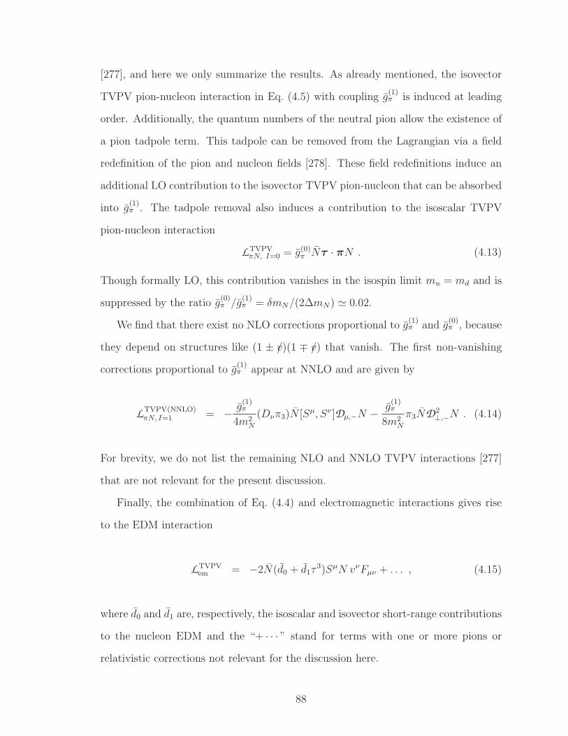
[277], and here we only summarize the results. As already mentioned, the isovector
TVPV pion-nucleon interaction in Eq. (4.5) with coupling g(1)π is induced at leading
order. Additionally, the quantum numbers of the neutral pion allow the existence of
a pion tadpole term. This tadpole can be removed from the Lagrangian via a field
redefinition of the pion and nucleon fields [278]. These field redefinitions induce an
additional LO contribution to the isovector TVPV pion-nucleon that can be absorbed
into g(1)π . The tadpole removal also induces a contribution to the isoscalar TVPV
pion-nucleon interaction
LTVPVπN, I=0 = g(0)
π Nτ · πN . (4.13)
Though formally LO, this contribution vanishes in the isospin limit mu = md and is
suppressed by the ratio g(0)π /g
(1)π = δmN/(2∆mN) ≃ 0.02.
We find that there exist no NLO corrections proportional to g(1)π and g
(0)π , because
they depend on structures like (1 ± v/)(1 ∓ v/) that vanish. The first non-vanishing
corrections proportional to g(1)π appear at NNLO and are given by
LTVPV(NNLO)πN, I=1 = − g
(1)π
4m2N
(Dνπ3)N [Sµ, Sν ]Dµ,−N − g(1)π
8m2N
π3ND2⊥,−N . (4.14)
For brevity, we do not list the remaining NLO and NNLO TVPV interactions [277]
that are not relevant for the present discussion.
Finally, the combination of Eq. (4.4) and electromagnetic interactions gives rise
to the EDM interaction
LTVPVem = −2N(d0 + d1τ
3)SµN vνFµν + . . . , (4.15)
where d0 and d1 are, respectively, the isoscalar and isovector short-range contributions
to the nucleon EDM and the “+ · · · ” stand for terms with one or more pions or
relativistic corrections not relevant for the discussion here.
88
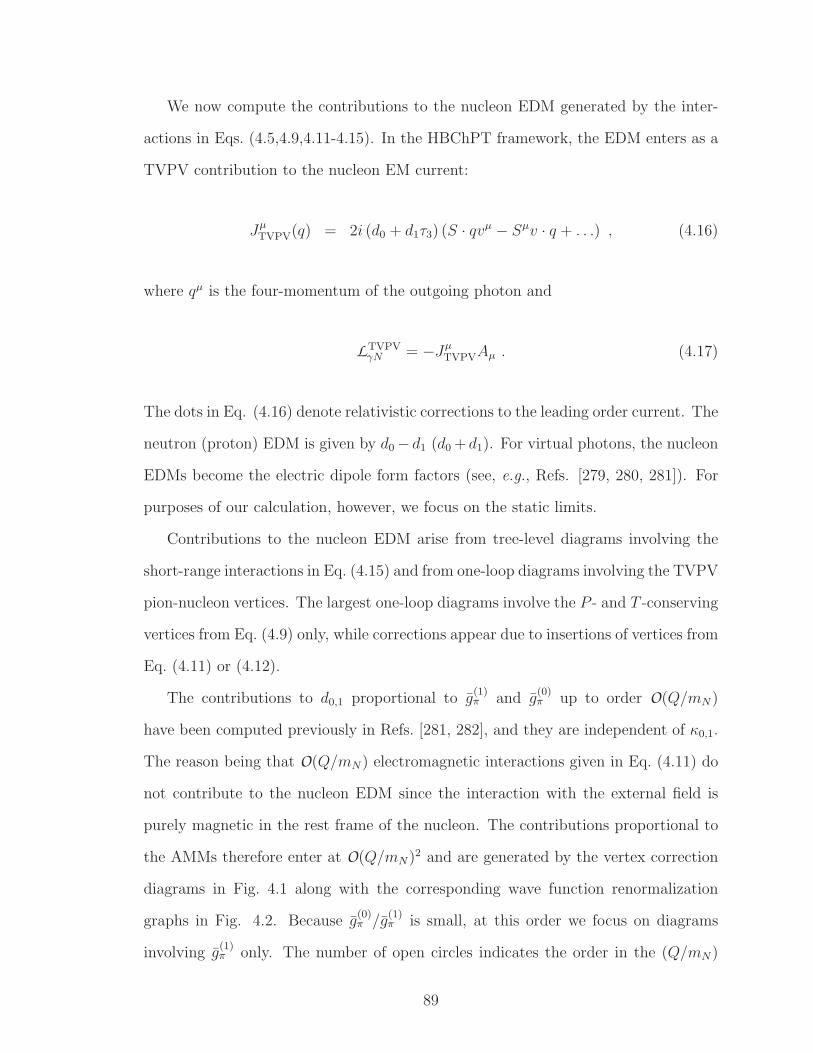
We now compute the contributions to the nucleon EDM generated by the inter-
actions in Eqs. (4.5,4.9,4.11-4.15). In the HBChPT framework, the EDM enters as a
TVPV contribution to the nucleon EM current:
JµTVPV(q) = 2i (d0 + d1τ3) (S · qvµ − Sµv · q + . . .) , (4.16)
where qµ is the four-momentum of the outgoing photon and
LTVPVγN = −Jµ
TVPVAµ . (4.17)
The dots in Eq. (4.16) denote relativistic corrections to the leading order current. The
neutron (proton) EDM is given by d0 − d1 (d0 + d1). For virtual photons, the nucleon
EDMs become the electric dipole form factors (see, e.g., Refs. [279, 280, 281]). For
purposes of our calculation, however, we focus on the static limits.
Contributions to the nucleon EDM arise from tree-level diagrams involving the
short-range interactions in Eq. (4.15) and from one-loop diagrams involving the TVPV
pion-nucleon vertices. The largest one-loop diagrams involve the P - and T -conserving
vertices from Eq. (4.9) only, while corrections appear due to insertions of vertices from
Eq. (4.11) or (4.12).
The contributions to d0,1 proportional to g(1)π and g
(0)π up to order O(Q/mN)
have been computed previously in Refs. [281, 282], and they are independent of κ0,1.
The reason being that O(Q/mN) electromagnetic interactions given in Eq. (4.11) do
not contribute to the nucleon EDM since the interaction with the external field is
purely magnetic in the rest frame of the nucleon. The contributions proportional to
the AMMs therefore enter at O(Q/mN)2 and are generated by the vertex correction
diagrams in Fig. 4.1 along with the corresponding wave function renormalization
graphs in Fig. 4.2. Because g(0)π /g
(1)π is small, at this order we focus on diagrams
involving g(1)π only. The number of open circles indicates the order in the (Q/mN)
89
(a) (b) (c) (d)
Figure 4.1. One-loop diagrams contributing to the nucleon EDMs at next-to-next-to-leading order. Solid, dashed and wavy lines represent the propagation of nucleons,pions and photons, respectively. A square marks the isovector TVPV interactionfrom Eq. (4.5), other vertices representing the T- and P-conserving interactions.Each circle on the vertex represents a suppression factor proportional to 1/mN . Forsimplicity only one possible ordering is shown.
Figure 4.2. One-loop diagrams contributing to wave function renormalization. Thenotation is as in Fig. 4.1.
expansion. Again, because the O(Q/mN) electromagnetic interactions are purely
magnetic, the contributions from the topologies of Figs. 4.1(a-c) vanish individually.
We also find that the sum of contributions proportional to g(1)π that arise from the
O(Q/mN)2 wave function renormalization vanish. The only surviving, non-vanishing
contribution is generated by the topology of Fig. 4.1(d).
At O(Q/mN)2, an additional set of contributions to the proton EDM proportional
to g(1)π are generated by the graphs in Fig. 4.3. The latter contain only the coupling
to the nucleon charge and various combinations of (a) O(Q/mN) corrections to the
πNN interactions and nucleon propagator as well as (b) O(Q/mN)2 corrections to one
of the couplings or propagator and LO interactions for the remaining components of
the diagram. Finally, at this order in principle contributions appear due to two-loop
diagrams involving g(1)π and LO P - and T -conserving vertices. However, the sum of
these diagrams vanishes.
90
(a) (b) (c)
Figure 4.3. Representative one-loop diagrams contributing at order (mπ/mN)2 to
the proton EDM proportional to g(1)π and independent of the anomalous magnetic
moment coupling. The notation is as in Fig. 4.1.
Before giving our result, we first quote the LO and NLO results, including the
contributions involving both g(1)π and g
(0)π . It should be noted that the results involv-
ing g(0)π are actually suppressed by the smallness of g
(0)π /g
(1)π for the CPV source in
Eq. (4.4). The LO contribution proportional to g(0)π has been first calculated in Ref.
[282], while the NLO corrections have been calculated in Refs. [281]. Together they
give
dLO+NLO0 = d0 −
egA
4π2Fπ
πmπ
4mN
(
3g(0)π + g(1)
π
)
,
dLO+NLO1 = d1 −
egA
4π2Fπ
[
g(0)π
(
L− lnm2
π
µ2+
5π
4
mπ
mN
)
+π
4
mπ
mN
g(1)π
]
. (4.18)
The contribution of g(0)π to the isovector EDM is UV divergent, with divergence en-
coded in the factor
L ≡ 2
4 − d− γE + ln 4π , (4.19)
in terms of number of space-time dimensions d and the Euler-Mascheroni constant
γE. The divergence is absorbed by the low-energy constant d1, which also contains
an a priori unknown non-vanishing finite contribution. It is conventional to absorb
L entirely into d1, thereby isolating the terms non-analytic in quark mass that are
unique to the loops. Notice that, at this order, the g(1)π terms do not contribute to
91
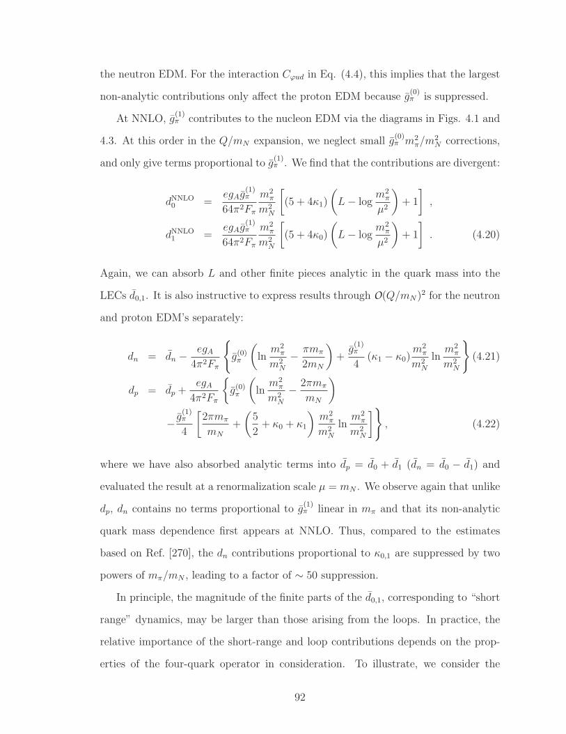
the neutron EDM. For the interaction Cϕud in Eq. (4.4), this implies that the largest
non-analytic contributions only affect the proton EDM because g(0)π is suppressed.
At NNLO, g(1)π contributes to the nucleon EDM via the diagrams in Figs. 4.1 and
4.3. At this order in the Q/mN expansion, we neglect small g(0)π m2
π/m2N corrections,
and only give terms proportional to g(1)π . We find that the contributions are divergent:
dNNLO0 =
egAg(1)π
64π2Fπ
m2π
m2N
[
(5 + 4κ1)
(
L− logm2
π
µ2
)
+ 1
]
,
dNNLO1 =
egAg(1)π
64π2Fπ
m2π
m2N
[
(5 + 4κ0)
(
L− logm2
π
µ2
)
+ 1
]
. (4.20)
Again, we can absorb L and other finite pieces analytic in the quark mass into the
LECs d0,1. It is also instructive to express results through O(Q/mN)2 for the neutron
and proton EDM’s separately:
dn = dn − egA
4π2Fπ
g(0)π
(
lnm2
π
m2N
− πmπ
2mN
)
+g
(1)π
4(κ1 − κ0)
m2π
m2N
lnm2
π
m2N
(4.21)
dp = dp +egA
4π2Fπ
g(0)π
(
lnm2
π
m2N
− 2πmπ
mN
)
− g(1)π
4
[
2πmπ
mN
+
(
5
2+ κ0 + κ1
)
m2π
m2N
lnm2
π
m2N
]
, (4.22)
where we have also absorbed analytic terms into dp = d0 + d1 (dn = d0 − d1) and
evaluated the result at a renormalization scale µ = mN . We observe again that unlike
dp, dn contains no terms proportional to g(1)π linear in mπ and that its non-analytic
quark mass dependence first appears at NNLO. Thus, compared to the estimates
based on Ref. [270], the dn contributions proportional to κ0,1 are suppressed by two
powers of mπ/mN , leading to a factor of ∼ 50 suppression.
In principle, the magnitude of the finite parts of the d0,1, corresponding to “short
range” dynamics, may be larger than those arising from the loops. In practice, the
relative importance of the short-range and loop contributions depends on the prop-
erties of the four-quark operator in consideration. To illustrate, we consider the
92
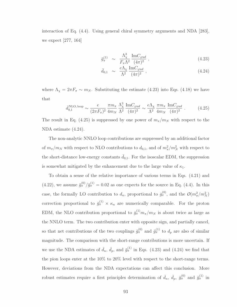
interaction of Eq. (4.4). Using general chiral symmetry arguments and NDA [283],
we expect [277, 164]
g(1)π ∼
Λ3χ
FπΛ2
ImCϕud
(4π)2, (4.23)
d0,1 ∼ eΛχ
Λ2
ImCϕud
(4π)2, (4.24)
where Λχ = 2πFπ ∼ mN . Substituting the estimate (4.23) into Eqs. (4.18) we have
that
dNLO, loop0,1 ∼ e
(2πFπ)2
πmπ
4mN
Λ3χ
Λ2
ImCϕud
(4π)2∼ eΛχ
Λ2
πmπ
4mN
ImCϕud
(4π)2. (4.25)
The result in Eq. (4.25) is suppressed by one power of mπ/mN with respect to the
NDA estimate (4.24).
The non-analytic NNLO loop contributions are suppressed by an additional factor
of mπ/mN with respect to NLO contributions to d0,1, and of m2π/m
2N with respect to
the short-distance low-energy constants d0,1. For the isoscalar EDM, the suppression
is somewhat mitigated by the enhancement due to the large value of κ1.
To obtain a sense of the relative importance of various terms in Eqs. (4.21) and
(4.22), we assume g(0)π /g
(1)π = 0.02 as one expects for the source in Eq. (4.4). In this
case, the formally LO contribution to dn, proportional to g(0)π , and the O(m2
π/m2N)
correction proportional to g(1)π × κn are numerically comparable. For the proton
EDM, the NLO contribution proportional to g(1)π mπ/mN is about twice as large as
the NNLO term. The two contribution enter with opposite sign, and partially cancel,
so that net contributions of the two couplings g(0)π and g
(1)π to dp are also of similar
magnitude. The comparison with the short-range contributions is more uncertain. If
we use the NDA estimates of dn, dp, and g(1)π in Eqs. (4.23) and (4.24) we find that
the pion loops enter at the 10% to 20% level with respect to the short-range terms.
However, deviations from the NDA expectations can affect this conclusion. More
robust estimates require a first principles determination of dn, dp, g(0)π and g
(1)π in
93
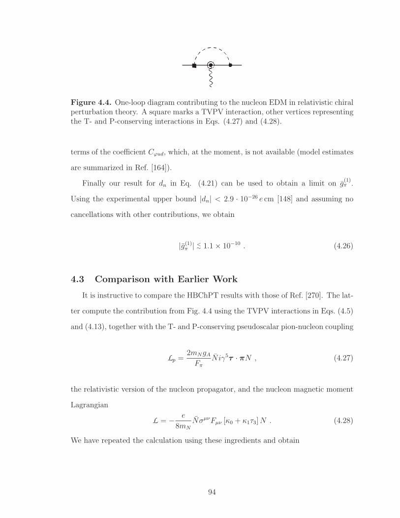
Figure 4.4. One-loop diagram contributing to the nucleon EDM in relativistic chiralperturbation theory. A square marks a TVPV interaction, other vertices representingthe T- and P-conserving interactions in Eqs. (4.27) and (4.28).
terms of the coefficient Cϕud, which, at the moment, is not available (model estimates
are summarized in Ref. [164]).
Finally our result for dn in Eq. (4.21) can be used to obtain a limit on g(1)π .
Using the experimental upper bound |dn| < 2.9 · 10−26 e cm [148] and assuming no
cancellations with other contributions, we obtain
|g(1)π | <∼ 1.1 × 10⁻¹⁰ . (4.26)
4.3 Comparison with Earlier Work
It is instructive to compare the HBChPT results with those of Ref. [270]. The lat-
ter compute the contribution from Fig. 4.4 using the TVPV interactions in Eqs. (4.5)
and (4.13), together with the T- and P-conserving pseudoscalar pion-nucleon coupling
Lp =2mNgA
Fπ
Niγ5τ · πN , (4.27)
the relativistic version of the nucleon propagator, and the nucleon magnetic moment
Lagrangian
L = − e
8mN
NσµνFµν [κ0 + κ1τ3]N . (4.28)
We have repeated the calculation using these ingredients and obtain
94
d0 = e(3g(0)π κ0 + g(1)
π κ1)gA
16π2Fπ
FP
(
m2π
m2N
)
,
d1 = e(−g(0)π κ1 + g(1)
π κ0)gA
16π2Fπ
FP
(
m2π
m2N
)
, (4.29)
where, when expanded for small x,
FP (x) =3
2
[
4
3− 2
3π√x− x log x+ O(x3/2)
]
. (4.30)
The result obtained in Ref. [270] is similar apart from the first term in Eq. (4.30)
that is 1 in their work instead of 4/3 as we find. The discrepancy can be traced back
to a term containing the product of Dirac matrices γασµνγα. This combination is
proportional to d− 4, but comes in front of a divergent integral. In the limit d→ 4,
the 1/(d−4) from the loop integral cancels the d−4 in the product of Dirac matrices,
leaving a constant piece.
Comparing with the HBChPT results in Eq. (4.20), we see that the relativistic
calculation with pseudoscalar coupling yields contributions proportional to g(1)π κ0,1
that arise at lower order in mπ/mN . The zeroth order term in Eq. (4.29) clearly
conflicts with the power counting expected in a well-behaved EFT since there ap-
pears no mπ/mN suppression. Using Eq. (4.23) in Eq. (4.29) would conflict with
the chiral/NDA expectations in Eq. (4.25), overestimating the latter by a factor of
mN/mπ ∼ 10.
The term non-analytic in the quark mass (mπ ∼ √mu,d) proportional to (mπ/mN)κ0,1
in Eq. (4.29) respects, in principle, the chiral/NDA estimate, but in the HBChPT
calculation this term is absent. We can trace this discrepancy back to the use of
the pseudoscalar coupling in Eq. (4.27) which breaks chiral symmetry. Repeating
the calculation with the relativistic axial-vector pion-nucleon coupling that conserves
chiral symmetry, we find that the (mπ/mN)κ0,1 term does not appear. The first non-
analytic terms that appear are then proportional to (m2π/m
2N)κ0,1, as they should
95
be. We refrain from giving all details, but have confirmed that by using appropriate
matching conditions the non-analytic terms appearing in the HBChPT and relativis-
tic calculation (with axial-vector pion-nucleon coupling) are the same6. Of course,
in the relativistic calculation with pseudovector coupling there still appear analytic
terms that are lower order in mπ/mN that may overestimate the dependence of the
nucleon EDM on g(0)π and g
(1)π .
4.4 Implications and Conclusions
From the foregoing discussion, it is evident that any phenomenological constraints
obtained from experimental limits on dn and the results in Eq. (4.29) are likely to
be at least an order of magnitude too stringent. In HBChPT, the loop contributions
proportional to κ0,1 arise at NNLO in the Q/mN expansion, while κ-independent
contributions start off at NLO. For the isoscalar EDM, the NNLO contribution is
numerically comparable to the NLO term due to the large magnitude of κ1, whereas
for the neutron the NLO contribution is absent and the NNLO suppression is more
severe. In terms of the “left-right symmetric” four-quark interaction (4.4), the NLO
loop contributions and the chiral/NDA estimates for the short distance LEC are nu-
merically comparable although the loops can be expected to be somewhat smaller
due to to a mπ/mN suppression. Consequently, we see no reasonable way around the
mπ/mN suppression that should be applied to the analysis of the LRSM. For other
scenarios that lead to a different subset of the d = 6 CPV operators, such as the
Weinberg operator or chiral invariant four-quark operators, the loop contributions
associated with g(1)π will be further suppressed compared to the short distance contri-
6The chiral symmetry-breaking impact of the pseudoscalar coupling enters through the tree-level,parity-conserving, pion-photon production sub-graphs of the one-loop TVPV diagrams. Matchingonto the HBChPT Lagrangian requires introduction of an explicit chiral symmetry-breaking opera-tor. No such operator is required when matching with the relativistic, pseudovector calculation.
96
butions. On the other hand, a scenario in which the isovector quark chromo-EDM is
the dominant d = 6 CPV source will have a similar phenomenology as the LRSM7.
For the LRSM with spontaneous CPV, the relaxed constraints may allow for
consistency between EDMs, the kaon CPV parameter ǫ, and a right-handed W -boson
(WR) with mass of a few TeV rather than the lower bound of 10 TeV quoted in
Ref. [267] (see the right panel of Fig. 8 for an illustration of the impact of relaxed
EDM constraints). In this case, discovery of the WR at the Large Hadron Collider
would still be possible, though it would likely imply that a second neutral CP-even
Higgs boson would be too heavy to be observed.
Similar conclusions apply to the analysis of Ref. [269] that considered the im-
plications of dn limits for the P-conserving, T-violating neutron decay correlation
~J · ~pe × ~pν with a coefficient denoted by D. Separating out the final state interactions
(Df ) that can mimic bona fide T-violation (Dt), the authors of Ref. [269] use the
work of Ref. [268] that, in turn, relied one the relativistic meson theory calculation of
Ref. [270], to conclude that |Dt/κ| < 10−7, where κ denotes the combination of Fermi
and Gamow-Teller matrix elements, gA, and the vector coupling gV that enters the
correlation. This bound lies well below the computed final state interaction contri-
bution |Dfκ| ∼ 10−5 with an uncertainty at the 10−7 level. In this case, it would not
be possible to disentangle final state contributions from possible LRSM contributions
for experiment performed with 10−7 level sensitivity. However, applying the relaxed
EDM constraint we obtain here would lead to |Dt/κ| < 10−6, opening a window for
a future D-correlation experiment to observe a non-vanishing LRSM effect.
7Deviations from these expectations might appear in the EDMs of multi-nucleon systems [277].
97
CHAPTER 5
REEXAMINATION OF THE STANDARD MODEL
NUCLEON ELECTRIC DIPOLE MOMENT
The search for permanent electric dipole moment (EDM) of elementary and com-
posite particles is motivated by its CP-violating nature. We live in a universe in which
the amount of baryons and antibaryons are unequal. In order to explain this asym-
metry CP-violating interactions are needed to fulfill one of the three Sakharov criteria
[38]. EDMs of elementary and composite particles are, in most cases, direct conse-
quences of these interactions which can be probed in low-energy experiments. Since
the first upper limit on the neutron EDM obtained by Smith, Purcell and Ramsey
in 1957 [33], numerous experiments have been performed to improve the sensitivity
of EDM measurements in different particle systems. Currently, the most stringent
bounds on EDMs are set for the electron (8.7 × 10⁻²⁹e cm, 90% C.L.)[146] and the
mercury atom (3.1×10⁻²⁹e cm, 95% C.L.)[147], while the current upper limit on neu-
tron and proton EDMs are 2.9×10⁻²⁶e cm (90% C.L.)[148] and 7.9×10⁻²⁵e cm (95%
C.L.) respectively (the latter is deduced from the bound on the mercury EDM). Fu-
ture experiments are designed (or have been considered) to push these bounds even
further down. For the neutron EDM, this includes the experiment at Paul Scher-
rer Institut (PSI)[149], the CryoEDM and PNPI/ILL experiment at Institut Laue-
Langevin (ILL)[150], the SNS neutron EDM experiment at Oak Ridge, the TRIUMF
experiment in Canada and the Munich experiment at Germany. These experiments
0Reprinted article with permission from C. Y. Seng, Phys. Rev. C 91 (2015)no.2, 025502. Copyright (2014) by the American Physical Society. DOI:http://dx.doi.org/10.1103/PhysRevC.91.025502
98
are designed to reach a 10−28e cm precision level for the neutron EDM [151]. Also,
both COSY[152] and BNL[153] have proposed storage ring experiments designed to
measure the proton EDM to a level of 10−29e cm precision.
Although numerous Beyond Standard Model (BSM) scenarios have been proposed
that give rise to measurable EDMs within current experimental precision level, so
far no definitive signal of such physics has been observed 1. Therefore, the CP-
violating phase of the Cabibbo-Kobayashi-Maskawa (CKM) matrix in the Standard
Model (SM) remains the only source for intrinsic EDMs. Questions have been raised
concerning the expected size of EDMs coming from purely SM physics[154]. A simple
dimensional analysis using constituent quark masses may suggest that the SM-induced
neutron EDM could be as large as 10−29e cm, approaching the level of sensitivity for
future EDM experiments. It is therefore important to have a better estimate for the
SM contribution to the nucleon EDM. To leading order, the quark EDM induced by
the CKM matrix starts at three-loops [155]. A detailed calculation showed that the
valence-quark contribution to the neutron EDM is of order 10−34e cm [156]. It was
also shown that long-distance contributions, namely contributions with baryons and
mesons as effective degrees of freedom (DOFs), could generate a much larger hadronic
EDM. For instance, the pion-loop contribution to the neutron EDM was first studied
in a paper by Barton and White [157] which produced log-divergent results in the
chiral limit indicating that the long-range contribution may dominate. On the other
hand, in a series of papers, Gavela et.al. studied the pole-diagram contribution with
the CP-violating phase generated by |∆S| = 1 electroweak [158] and gluonic penguin
diagrams [159]. They claimed that the latter is dominant and derived a SM neutron
EDM of order 10−31e cm. The possibility of a long-range contribution to the neutron
1There are indeed some hopeful candidates, for example the muon g−2 anomaly; but no conclusivestatement can be made before one could further improve the experimental precision and reduce thetheoretical uncertainty of the SM prediction.
99
EDM from the CKM matrix was first pointed out by Khriplovich and Zhitnitsky[160].
He et.al [161] did a thorough chiral-loop calculation and re-analyzed the pole-diagram
contribution in [158, 159] and argued that the two are of the same order of magnitude.
Their estimate for the neutron EDM is 1.6 × 10⁻³¹e cm − 1.4 × 10⁻³³e cm, which is
currently the most widely accepted estimate for the SM neutron EDM. In recent
years, the charm contribution to nucleon EDMs is also considered and it is roughly
10−31e cm [162].
The purpose of this paper is to revisit the previous study of both chiral-loop and
the pole contributions to the nucleon EDM in order to sharpen our SM benchmark
value. On the theoretical side, one could improve earlier work in several ways. For
instance, the chiral loop calculation in [161] adopted an older meson theory utilizing a
pseudoscalar strong baryon-meson coupling that should be replaced by the standard
axial-vector coupling. Also, their work that utilized an effective hadronic Lagrangian
in computing chiral-loop diagrams faced another well-known problem in the loss of
power counting similar to that happening in the relativistic Chiral Perturbation The-
ory (ChPT). ChPT is a non-renormalizable theory that involves infinitely many inter-
action terms. Its predictive power therefore relies on the fact that higher order terms
are suppressed by powers of p/Λχ where p is the typical mass or momentum scales
of hadronic DOFs and Λχ ∼ 1GeV. This expansion however becomes ambiguous
when baryons are included because a typical baryon mass is MB ∼ 1GeV. Therefore,
MB/Λχ is no longer a small expansion parameter. Heavy Baryon Chiral Perturbation
Theory (HBchPT) [163] provides a convincing way to get around this issue by per-
forming a field redefinition in the baryon field to scale out its mass-dependence. By
doing this, one can split the baryon field into “light” and “heavy” components, where
the former depends only on its residual momentum which is well below 1 GeV. After
integrating out the heavy component of the baryon field, the effective Lagrangian
can be written as a series expansion of 1/mN . This eliminates the possibility of a
100
factor mN appearing in the numerator and thus restores the power counting. Many
works have appeared recently calculating the nucleon EDM induced by different BSM
physics using HBchPT (see [164] for a general overview). Although the convergence
of the SU(3) HBchPT is not as good as its SU(2) counterpart because mK/mN is not
very small [165, 166, 167, 168, 169], it is still theoretically beneficial as it provides
a formal classification of different contributions into leading and sub-leading orders.
In this work, the chiral-loop contribution to the nucleon EDM are recalculated up to
the leading-order (LO) in the heavy baryon (HB)-expansion.
Additionally, previous numerical results of loop and pole contributions face large
uncertainties due to poorly-known values of physical constants in the weak sector at
that time. For example, the CP-violating phase δ of the CKM matrix quoted in Ref.
[161] had an uncertainty that spans one order of magnitude. The fitting of certain low
energy constants (LECs) such as weak baryon-meson interaction strengths, has been
updated since. Also, their theoretical estimation of various CP-phases in the effective
weak Lagrangian was based on older work [170, 171] which had been improved by
others. Furthermore, for previous work on pole contributions, their estimation on
effective CP-phases was based only on a single gluonic penguin operator without
considering the full analysis of operator mixing and renormalization group running.
Moreover, the approximate form of their analytic expressions was based on the out-
of-date assumption that mt ≪ mW . In this work, I do a more careful determination
of weak LECs, taking all these issues into account. Combining my calculation and an
estimate of higher-order effects, I predict a range of the long-distance SM contribution
to the nucleon EDM to be around (1− 6)× 10−32e cm. I identify the main sources of
uncertainty and discuss possible steps one could take to improve upon that. At the
same time, I use dimensional analysis to estimate the size of possible short-distance
counterterms. I find that they could be as large as 4 × 10⁻³²e cm.
101
This work is arranged as follows: in Section II I will briefly outline the main
ingredients of the SU(3) HBchPT and introduce the weak Lagrangian responsible for
the generation of the nucleon EDM. In Section III I will determine the LECs. In
Section IV and V Iderive the analytic expressions for loop and pole contributions to
the nucleon EDM respectively and calculate their numerical values. In Section VI I
will provide some further discussions and draw my conclusions.
5.1 HBchPT: Strong and Electroweak Interactions
In this section, I review some basic concepts of ChPT with the primary aim of
establishing conventions and notation. ChPT is a low-energy effective field theory
(EFT) of quantum chromodynamics (QCD) with hadrons as low energy DOFs. QCD
exhibits a global chiral symmetry in the limit of massless quarks. However this sym-
metry is spontaneously broken in the ground state and leads to the emergence of
Goldstone bosons which are identified as pseudoscalar mesons. The corresponding
EFT obeys the same symmetry. An infinite tower of operators respecting the symme-
try with increasing mass dimensions is organized in the Lagrangian. However, only
a finite number of operators are retained since the the dropped higher-dimensional
operators make contributions that are suppressed by powers of p/Λχ.
I use the standard non-linear representation of chiral fields [172, 174, 173], in
which the pseudoscalar meson octet is incorporated in the exponential function U =
expiφ/Fπ, where
φ =8∑
a=1
φaλa =
π0 + 1√3η8
√2π+
√2K+
√2π− −π0 + 1√
3η8
√2K0
√2K− √
2K0 −23η8
(5.1)
with Fπ ≈ 93MeV. The matrix U transforms under the chiral rotation as: U → LUR†,
where L and R are elements of SU(3)L and SU(3)R respectively. The mass term of
102
the meson octet is introduced using spurion analysis: the QCD Lagrangian would
exhibit chiral invariance if the quark mass matrix M = diagmu,md,ms transforms
as M → LMR†. Therefore, its low energy effective theory written in terms of the
spurion field M should also exhibit a similar invariance. The lowest-order operator
that is invariant is Tr[MU †+UM †]. This operator gives rise to non-zero meson masses
which are isospin-symmetric.
The ground state JP = (1/2)+ baryon octet is assembled into the matrix:
B =
Σ0√2
+ Λ√6
Σ+ p
Σ− −Σ0√2
+ Λ√6
n
Ξ− Ξ0 − 2Λ√6
. (5.2)
It transforms as: B → KBK† with K = K(L,R, U) being a unitary matrix. In order
to couple baryons with the pseudoscalar octet, we define ξ =√U which transforms
as ξ → LξK† = KξR† and introduce the Hermitian axial vector:
Aµ =i
2[ξ∂µξ
† − ξ†∂µξ] (5.3)
which transforms as Aµ → KAµK† under the chiral rotation (we have neglected its
coupling with external fields because it is not needed in this work).
I now proceed with with the formulation of HBchPT. In order to scale out the
heavy mass-dependence, I rewrite its momentum as
pµ = mNvµ + kµ, (5.4)
where mN is the nucleon mass, vµ is the velocity of the baryon (which is conserved
in the mN → ∞ limit) and kµ is the residual momentum of the baryon which is well
103
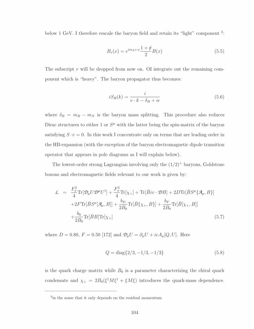
below 1 GeV. I therefore rescale the baryon field and retain its “light” component 2:
Bv(x) = eimNv·x 1 + v/
2B(x) (5.5)
The subscript v will be dropped from now on. OI integrate out the remaining com-
ponent which is “heavy”. The baryon propagator thus becomes:
iSB(k) =i
v · k − δB + iǫ(5.6)
where δB = mB − mN is the baryon mass splitting. This procedure also reduces
Dirac structures to either 1 or Sµ with the latter being the spin-matrix of the baryon
satisfying S ·v = 0. In this work I concentrate only on terms that are leading order in
the HB-expansion (with the exception of the baryon electromagnetic dipole transition
operator that appears in pole diagrams as I will explain below).
The lowest-order strong Lagrangian involving only the (1/2)+ baryons, Goldstone
bosons and electromagnetic fields relevant to our work is given by:
L =F 2
π
4Tr[DµUDµU †] +
F 2π
4Tr[χ+] + Tr[Biv · DB] + 2DTr[BSµAµ, B]
+2FTr[BSµ[Aµ, B]] +bD2B0
Tr[Bχ+, B] +bF2B0
Tr[B[χ+, B]]
+b0
2B0
Tr[BB]Tr[χ+] (5.7)
where D = 0.80, F = 0.50 [172] and DµU = ∂µU + ieAµ[Q,U ]. Here
Q = diag2/3,−1/3,−1/3 (5.8)
is the quark charge matrix while B0 is a parameter characterizing the chiral quark
condensate and χ+ = 2B0(ξ†Mξ† + ξMξ) introduces the quark-mass dependence.
2in the sense that it only depends on the residual momentum
104
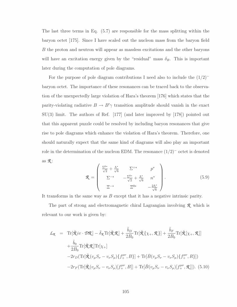
The last three terms in Eq. (5.7) are responsible for the mass splitting within the
baryon octet [175]. Since I have scaled out the nucleon mass from the baryon field
B the proton and neutron will appear as massless excitations and the other baryons
will have an excitation energy given by the “residual” mass δB. This is important
later during the computation of pole diagrams.
For the purpose of pole diagram contributions I need also to include the (1/2)−
baryon octet. The importance of these resonances can be traced back to the observa-
tion of the unexpectedly large violation of Hara’s theorem [176] which states that the
parity-violating radiative B → B′γ transition amplitude should vanish in the exact
SU(3) limit. The authors of Ref. [177] (and later improved by [178]) pointed out
that this apparent puzzle could be resolved by including baryon resonances that give
rise to pole diagrams which enhance the violation of Hara’s theorem. Therefore, one
should naturally expect that the same kind of diagrams will also play an important
role in the determination of the nucleon EDM. The resonance (1/2)− octet is denoted
as R :
R =
Σ0∗√2
+ Λ∗√6
Σ+∗ p∗
Σ−∗ −Σ0∗√2
+ Λ∗√6
n∗
Ξ−∗ Ξ0∗ −2Λ∗√6
. (5.9)
It transforms in the same way as B except that it has a negative intrinsic parity.
The part of strong and electromagnetic chiral Lagrangian involving R which is
relevant to our work is given by:
LR = Tr[R iv · DR ] − δR Tr[R R ] +bD2B0
Tr[R χ+,R ] +bF2B0
Tr[R [χ+,R ]]
+b0
2B0
Tr[R R ]Tr[χ+]
−2rD(Tr[R (vµSν − vνSµ)fµν+ , B] + Tr[B(vµSν − vνSµ)fµν
+ , R])
−2rF (Tr[R (vµSν − vνSµ)[fµν+ , B]] + Tr[B(vµSν − vνSµ)[fµν
+ ,R ]]). (5.10)
105
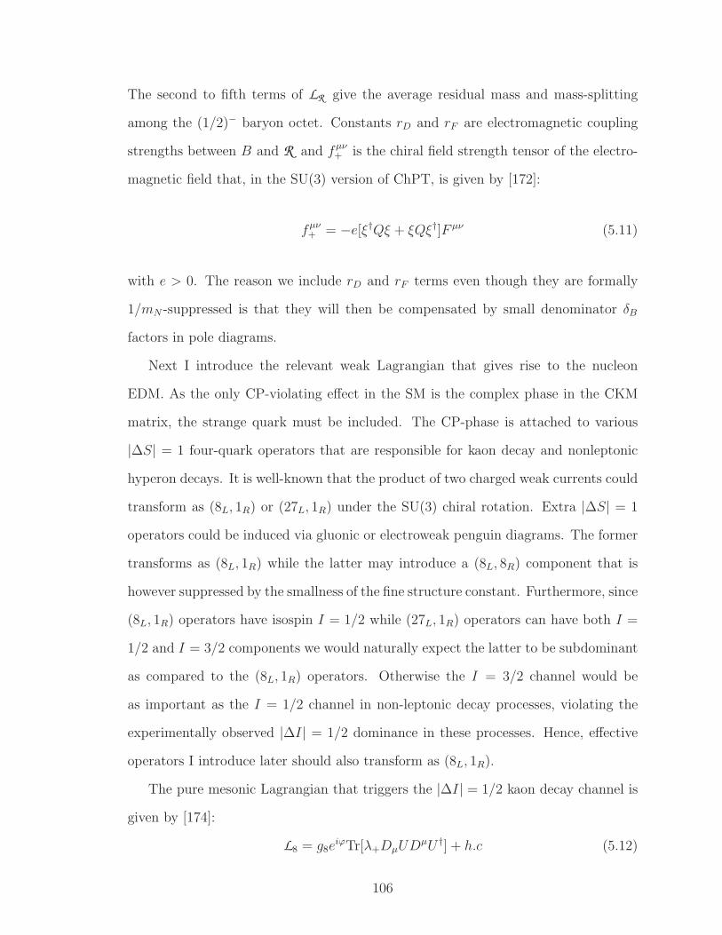
The second to fifth terms of LR give the average residual mass and mass-splitting
among the (1/2)− baryon octet. Constants rD and rF are electromagnetic coupling
strengths between B and R and fµν+ is the chiral field strength tensor of the electro-
magnetic field that, in the SU(3) version of ChPT, is given by [172]:
fµν+ = −e[ξ†Qξ + ξQξ†]F µν (5.11)
with e > 0. The reason we include rD and rF terms even though they are formally
1/mN -suppressed is that they will then be compensated by small denominator δB
factors in pole diagrams.
Next I introduce the relevant weak Lagrangian that gives rise to the nucleon
EDM. As the only CP-violating effect in the SM is the complex phase in the CKM
matrix, the strange quark must be included. The CP-phase is attached to various
|∆S| = 1 four-quark operators that are responsible for kaon decay and nonleptonic
hyperon decays. It is well-known that the product of two charged weak currents could
transform as (8L, 1R) or (27L, 1R) under the SU(3) chiral rotation. Extra |∆S| = 1
operators could be induced via gluonic or electroweak penguin diagrams. The former
transforms as (8L, 1R) while the latter may introduce a (8L, 8R) component that is
however suppressed by the smallness of the fine structure constant. Furthermore, since
(8L, 1R) operators have isospin I = 1/2 while (27L, 1R) operators can have both I =
1/2 and I = 3/2 components we would naturally expect the latter to be subdominant
as compared to the (8L, 1R) operators. Otherwise the I = 3/2 channel would be
as important as the I = 1/2 channel in non-leptonic decay processes, violating the
experimentally observed |∆I| = 1/2 dominance in these processes. Hence, effective
operators I introduce later should also transform as (8L, 1R).
The pure mesonic Lagrangian that triggers the |∆I| = 1/2 kaon decay channel is
given by [174]:
L8 = g8eiϕTr[λ+DµUD
µU †] + h.c (5.12)
106
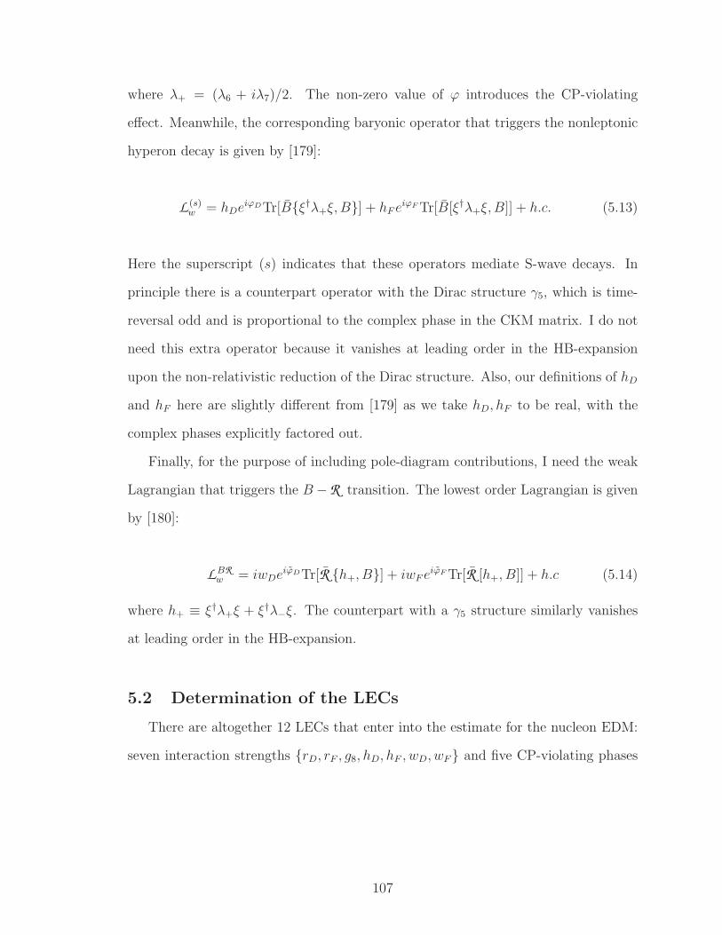
where λ+ = (λ6 + iλ7)/2. The non-zero value of ϕ introduces the CP-violating
effect. Meanwhile, the corresponding baryonic operator that triggers the nonleptonic
hyperon decay is given by [179]:
L (s)w = hDe
iϕDTr[Bξ†λ+ξ, B] + hF eiϕF Tr[B[ξ†λ+ξ, B]] + h.c. (5.13)
Here the superscript (s) indicates that these operators mediate S-wave decays. In
principle there is a counterpart operator with the Dirac structure γ5, which is time-
reversal odd and is proportional to the complex phase in the CKM matrix. I do not
need this extra operator because it vanishes at leading order in the HB-expansion
upon the non-relativistic reduction of the Dirac structure. Also, our definitions of hD
and hF here are slightly different from [179] as we take hD, hF to be real, with the
complex phases explicitly factored out.
Finally, for the purpose of including pole-diagram contributions, I need the weak
Lagrangian that triggers the B−R transition. The lowest order Lagrangian is given
by [180]:
LBRw = iwDe
iϕDTr[R h+, B] + iwF eiϕF Tr[R [h+, B]] + h.c (5.14)
where h+ ≡ ξ†λ+ξ + ξ†λ−ξ. The counterpart with a γ5 structure similarly vanishes
at leading order in the HB-expansion.
5.2 Determination of the LECs
There are altogether 12 LECs that enter into the estimate for the nucleon EDM:
seven interaction strengths rD, rF , g8, hD, hF , wD, wF and five CP-violating phases
107

ϕ, ϕD, ϕF , ϕD, ϕF. They are either extracted from experiments or obtained by
theoretical modeling 3.
Pure electromagnetic B−R transition coupling strengths rD and rF are fitted to
electromagnetic decays of (1/2)− resonances. The authors of Ref. [178] obtain:
erD = 0.033GeV−1, erF = −0.046GeV−1. (5.15)
The constant g8 is fitted to the K0s → π+π− decay rate, ignoring the small CP-
violating effect [181], giving
g8 = 6.84 × 10⁻¹⁰GeV2. (5.16)
The CP-phase ϕ is, up to a negative sign, the phase of the K0 → ππ(I = 0) decay
amplitude:
ϕ = −ξ0 = −ImA0
ReA0
(5.17)
In principle one could extract ξ0 from the measurement of the CP-violating parameter
ǫ′ in the kaon decay. However, ǫ′ is a linear combination of ξ0 and another CP-violating
phase, ξ2, of the I = 3/2 channel. Simple estimation [174] suggests that ξ2 is of the
same order as ξ0 making ξ0 hard to extract directly from the experiment. I therefore
refer to theoretical estimation based on the large-Nc approach [182] which gives:
ϕ = −ξ0 ≈ −√
2|ǫ| × (−6 × 10⁻²) ≈ 1.89 × 10⁻⁴ ≈ 6.4J, (5.18)
where J = (2.96+0.20−0.16) × 10−5 [181] is the Jarlskog invariant[183]. It is worthwhile to
mention that, in Ref. [161] the uncertainty of J spans an order of magnitude leading
3Unfortunately, none of these LECs in the literature come with error bars, so I cannot estimatethe error introduced by the fitting of LECs.
108
to the main source of the error in the estimate of the neutron EDM during that time.
Today, J is determined with much higher precision so the associated uncertainty is
sub-leading compared to uncertainties due to higher-order effects in the HB-expansion
and unknown short-distance counterterms, which we will discuss later.
The four remaining interaction strengths hD, hF , wD, wF were determined in [180]
by simultaneously fitting them to the s and p-wave amplitudes of nonleptonic hyperon
decays:
hD ≈ 0.44 × 10⁻⁷GeV
hF ≈ −0.50 × 10⁻⁷GeV
wD ≈ −1.8 × 10⁻⁷GeV
wF ≈ 2.3 × 10⁻⁷GeV. (5.19)
The last two constants were determined by setting mR ≈ 1535MeV.
Finally, I need to know the four remaining CP-phases ϕD, ϕF , ϕD, ϕF. These
phases have been considered in ref [158], but their treatments are less satisfactory due
to the neglect of the operator mixing effect and a certain outdated approximation of
the small top quark mass assumption. In order to improve upon that, I review a more
recent work done in Ref. [179] that determined ϕD, ϕF and apply scaling arguments
to provide an estimate of ϕD, ϕF. Ref. [179] pointed out that after considering
operator mixing and renormalization group running, the dominant operator that gives
rise to the CP-violating phase in the |∆S| = 1, |∆I| = 1/2 sector is given by:
Q6 = −2∑
q
d(1 + γ5)qq(1 − γ5)s. (5.20)
Ref [179] then computed the factorizable and non-factorizable contributions to ϕD, ϕF
induced by Q6. Here “factorizable” means to regard Q6 as a product of two chiral
109
quark densities and match it to chiral operators. The matching is done by realizing
that qRqL ∼ ∂LQCD/∂mq = ∂Lchiral/∂mq. On the other hand, the “non-factorizable”
contribution is obtained simply by taking the hadronic matrix element of Q6 using
the quark model. These two contributions are distinct because the factorizable piece
contains a factor of chiral quark condensate F 2πB0 through:
〈0| qiLq
jRq
kRq
lL
∣
∣BB′⟩ ∼ 〈0| qiLq
jR |0〉 〈0| qk
RqlL
∣
∣BB′⟩ = −1
2F 2
πB0δij 〈0| qkRq
lL
∣
∣BB′⟩
(5.21)
while the same quantity never appears in a quark model calculation. Combining
the two, they found Im(hD exp iϕD) ≈ −2.2, Im(hF exp iϕF ) ≈ 6.1, both in units of√
2FπGFm2π+J . This leads to:
ϕD ≈ −1.5J, ϕF ≈ −3.6J. (5.22)
It is straightforward to see that ϕD and ϕF receive no factorizable contribution.
This is because it would require terms like R mqB to appear in the strong chiral
Lagrangian. Such terms would violate parity and therefore cannot exist. For the non-
factorizable part, my strategy is the following: first I compute the matrix elements
〈R | Q6 |B〉 and 〈B′| Q6 |B〉 using the quark model to find their ratio. Then, I use
this ratio to infer the value of the non-factorizable part of ϕD, ϕF by appropriately
scaling the non-factorizable part of ϕD, ϕF given in Ref. [179].
To obtain an estimate of hadronic matrix elements I adopt the harmonic oscillator
model [177]. The structure of the spin-flavor wavefunction of the baryon octet leads
to the following ratio:
〈n∗| Q6
∣
∣Σ0⟩
: 〈n∗| Q6 |Λ〉 : 〈p∗| Q6
∣
∣Σ+⟩
= 1 :√
3 : −√
2 (5.23)
which requires that wF ϕF = (1/3)wDϕD in our chiral Lagrangian. I also obtain the
ratio between B −B′ and B − R matrix elements:
110
〈p∗| Q6 |Σ+〉〈p| Q6 |Σ+〉
= −√
2
3π
1
mR0
. (5.24)
where m ≈ 0.34GeV, R0 ≈ 2.7GeV−1 are harmonic oscillator parameters. With this
ratio and the non-factorizable contribution to ϕD, ϕF given in [179], I obtain the
non-factorizable contribution to ϕD, ϕF :
ϕD ≈ 0.04J, ϕF ≈ −0.01J (5.25)
These phases are about two orders of magnitude smaller than the three other CP-
phases because they are not enhanced by the chiral quark condensate. Therefore, I
disregard them in the rest of our calculation.
To end this section, I point out that there is an important sign issue in the deter-
mination of LECs. Since LECs are fitted to experiments that only involve squared
amplitudes, an overall undetermined sign is left ambiguous. Therefore, if two sets
of LECs are fitted separately to two unrelated experiments (for example, rD, rF
are to fit to baryon electromagnetic transitions and hD, hF , wD, wF are to fit to
non-leptonic hyperon decays), there is no unique way to determine the relative sign
between these two sets of LECs. This introduces an extra uncertainty because a
change of a relative sign can turn a constructive interference to destructive and vice
versa. I will discuss the impact of this uncertainty in the last section.
5.3 One loop contribution
In this section I present analytic and numerical results of the one-1oop contribution
to the proton and neutron EDM using HBchPT. The nucleon EDM dN is defined by
the term linear in the incoming photon momentum q of the P and T-violating NNγ
amplitude
111
iM ≡ −2dNv · εuNS · quN . (5.26)
Here εµ is the photon polarization vector. Note that the equation has been simplified
by applying the on-shell condition to the nucleon: v · q = −q2/2mN → 0.
Since each weak interaction vertex has |∆S| = 1, I need at least two insertions of
weak interaction vertices to obtain an EDM that is flavor diagonal. Most one-loop
integrals are UV-divergent and are regularized using the MS scheme in which the
combination
L ≡ 2
4 − d− γ + ln(4π) (5.27)
is subtracted. Also, since all CP-violating phases ϕi are small, I use the small angle
approximation sinϕi ≈ ϕi. Finally, following the usual spirit of ChPT, during the
calculation of loops we assume that the heavy DOFs could be integrated out and their
effects show up in the LECs of the effective operators consist of lighter DOFs 4. Hence
what enter the loops are the lightest DOFs, which in our case are the pseudoscalar
meson octet and the ground-state (1/2)+ baryon octet.
There are four distinct types of 1-loop diagrams (see Fig.5.1) that give non-zero
contribution to the nucleon EDM (diagrams of other kinds are all vanishing at leading
order in the HB-expansion. See the Appendix for the argument). Fig. 1(a)-(c) (plus
reflections) in Fig.5.1 contribute to both neutron and proton EDM. For the neutron,
it reads:
4The reader should anyway be alerted that this may not always be the case. For example, Ref.[186] pointed out that one needs to include the baryon decuplet in order to reconcile with the resultof the large Nc-expansion
112
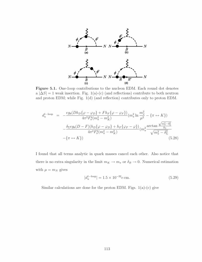
Figure 5.1. One-1oop contributions to the nucleon EDM. Each round dot denotesa |∆S| = 1 weak insertion. Fig. 1(a)-(c) (and reflections) contribute to both neutronand proton EDM; while Fig. 1(d) (and reflection) contributes only to proton EDM.
d1−loopn = −eg8(DhDϕ− ϕD + FhFϕ− ϕF)
4π2F 4π (m2
π −m2K)
(m2π ln
m2π
µ2− π ↔ K)
−δΣeg8(D − F )(hDϕ− ϕD + hFϕF − ϕ)4π2F 2
π (m2π −m2
K)(m2
π
arctan
√m2
π−δ2Σ
δΣ√
m2π − δ2
Σ
−π ↔ K) (5.28)
I found that all terms analytic in quark masses cancel each other. Also notice that
there is no extra singularity in the limit mK → mπ or δB → 0. Numerical estimation
with µ = mN gives
|d1−loopn | = 1.5 × 10⁻³²e cm. (5.29)
Similar calculations are done for the proton EDM. Figs. 1(a)-(c) give
113
d1−loop,1p =
eg8(DhD[ϕ− ϕD] + 3hF [ϕ− ϕF ] + 3FhD[ϕ− ϕD] + hF [ϕF − ϕ])24π2F 4
π (m2π −m2
K)
×(m2π ln
m2π
µ2− π ↔ K)
−δΣeg8(D − F )(hDϕ− ϕD + hFϕF − ϕ)8π2F 4
π (m2π −m2
K)(m2
π
arctan
√m2
π−δ2Σ
δΣ√
m2π − δ2
Σ
−π ↔ K)
−δΛeg8(D + 3F )(hDϕ− ϕD + 3hFϕ− ϕF)24π2F 4
π (m2π −m2
K)(m2
π
arctan
√m2
π−δ2Λ
δΛ√
m2π − δ2
Λ
−π ↔ K) (5.30)
There is one extra type of diagrams contributing to the proton EDM corresponding
to two insertions of hi vertices (Fig. 1(d)). The corresponding diagrams do not
generate the neutron EDM simply because there is no appropriate non-vanishing
combination of B,B′, φ. This diagram for the proton EDM gives
d1−loop,2p = −
ehDhF (D − F )(ϕD − ϕF )(π − 2 arctan δΣ√m2
K−δ2
Σ
)
16π2F 2π
√
m2K − δ2
Σ
−ehDhF (D + 3F )(ϕD − ϕF )(π − 2 arctan δΛ√
m2K−δ2
Λ
)
48π2F 2π
√
m2K − δ2
Λ
. (5.31)
This contribution is interesting since it is UV-finite. It depends non-analytically on
quark masses and hence uniquely characterizes long-distance physics 5. Numerically,
these give
|d1−loop,1p | = 6.1 × 10⁻³³e cm
|d1−loop,2p | = 1.1 × 10⁻³²e cm. (5.32)
5One can show that Eq. (5.31) remains real even when δK , δΛ > mK by using the identityarctan z = 1
2ilog 1+iz
1−iz.
114
I choose to present numerical results of d1−loop,1 and d1−loop,2 separately because the
former is proportional to g8hi while the latter is proportional to hihj. Since the
relative sign between g8 and hi is experimentally undetermined, these two terms can
either add or subtract each other.
As a short conclusion, I stress once again that within the HBchPT formalism,
my analytic results of 1-loop diagrams, Eq. (5.28), (5.30) and (5.31) fully respect
power counting as no powers of mB appear in the numerator upon carrying out loop
integrals. This is in contrast with the relativistic calculation done in Ref. [161], in
which the authors include diagrams involving MDM-like coupling that should have
an explicit 1/mB suppression according to the power counting, but is canceled by a
factor of mB appearing in the numerator coming from the loop integral.
Finally let me discuss the effect of counterterms. Since d1−loopn and d1−loop,1
p are
UV-divergent, I need to introduce corresponding counterterms d0n, d
0p to absorb the
infinities. These counterterms are generated by short-distance physics. Therefore
their precise values cannot be calculated. To estimate the size of these counterterms
we perform a naive dimensional analysis (NDA). Following [184], there are ten ∆S = 1
four-quark operators that mix under renormalization. The effective Hamiltonian can
be written as:
H∆S=1eff =
GF√2VudV
∗us
10∑
i=1
Ci(µ)Qi(µ) + h.c. (5.33)
Under conditions that ΛQCD ≈ 0.2GeV, µ = 1GeV and the top-quark mass mt =
174GeV, the largest flavor-diagonal CP-violating effect comes from the product of Q2
and Q6 with Wilson coefficients C2 = 1.31− 0.044τ and C6 = −0.011− 0.080τ where
τ = −VtdV∗ts/VudV
∗us. This gives:
d0p, d
0n ∼ 1
16π2
G2F
2|VudV
∗us|2Im(C2C
∗6)Λ3
χ ≈ 4 × 10⁻³²e cm. (5.34)
Here 1/16π2 is a necessary loop factor while the factor Λ3χ is included to achieve
the correct mass dimension. I choose Λχ ∼ 1GeV instead of some other scale like
115
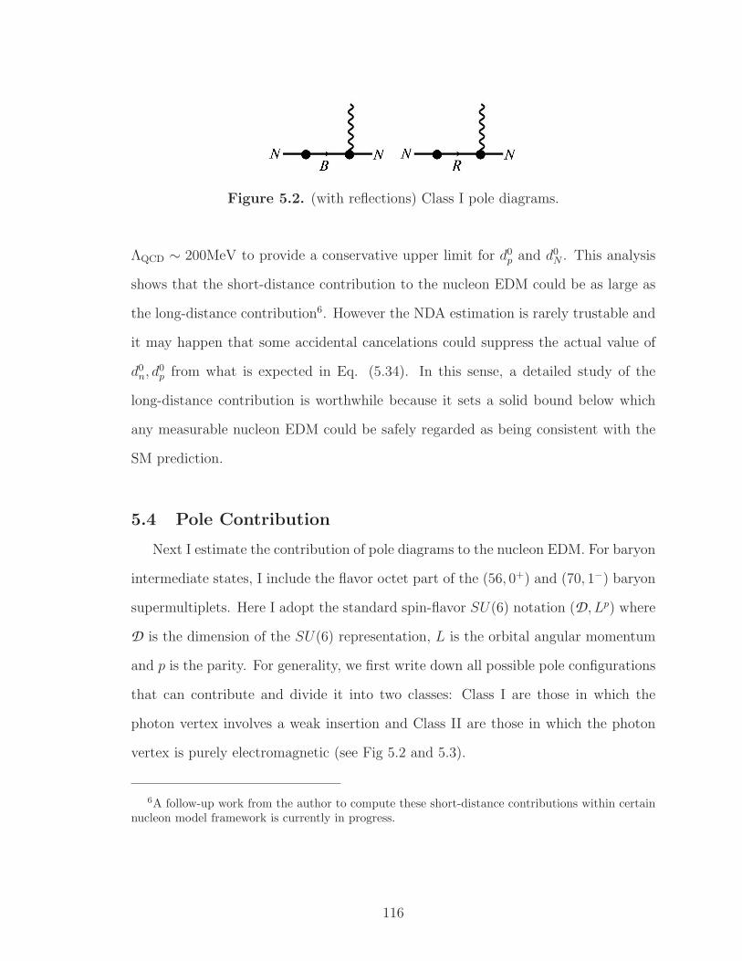
Figure 5.2. (with reflections) Class I pole diagrams.
ΛQCD ∼ 200MeV to provide a conservative upper limit for d0p and d0
N . This analysis
shows that the short-distance contribution to the nucleon EDM could be as large as
the long-distance contribution6. However the NDA estimation is rarely trustable and
it may happen that some accidental cancelations could suppress the actual value of
d0n, d
0p from what is expected in Eq. (5.34). In this sense, a detailed study of the
long-distance contribution is worthwhile because it sets a solid bound below which
any measurable nucleon EDM could be safely regarded as being consistent with the
SM prediction.
5.4 Pole Contribution
Next I estimate the contribution of pole diagrams to the nucleon EDM. For baryon
intermediate states, I include the flavor octet part of the (56, 0+) and (70, 1−) baryon
supermultiplets. Here I adopt the standard spin-flavor SU(6) notation (D, Lp) where
D is the dimension of the SU(6) representation, L is the orbital angular momentum
and p is the parity. For generality, we first write down all possible pole configurations
that can contribute and divide it into two classes: Class I are those in which the
photon vertex involves a weak insertion and Class II are those in which the photon
vertex is purely electromagnetic (see Fig 5.2 and 5.3).
6A follow-up work from the author to compute these short-distance contributions within certainnucleon model framework is currently in progress.
116
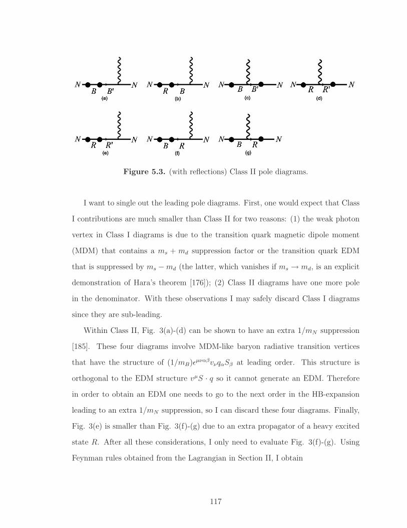
Figure 5.3. (with reflections) Class II pole diagrams.
I want to single out the leading pole diagrams. First, one would expect that Class
I contributions are much smaller than Class II for two reasons: (1) the weak photon
vertex in Class I diagrams is due to the transition quark magnetic dipole moment
(MDM) that contains a ms + md suppression factor or the transition quark EDM
that is suppressed by ms −md (the latter, which vanishes if ms → md, is an explicit
demonstration of Hara’s theorem [176]); (2) Class II diagrams have one more pole
in the denominator. With these observations I may safely discard Class I diagrams
since they are sub-leading.
Within Class II, Fig. 3(a)-(d) can be shown to have an extra 1/mN suppression
[185]. These four diagrams involve MDM-like baryon radiative transition vertices
that have the structure of (1/mB)ǫµναβvνqαSβ at leading order. This structure is
orthogonal to the EDM structure vµS · q so it cannot generate an EDM. Therefore
in order to obtain an EDM one needs to go to the next order in the HB-expansion
leading to an extra 1/mN suppression, so I can discard these four diagrams. Finally,
Fig. 3(e) is smaller than Fig. 3(f)-(g) due to an extra propagator of a heavy excited
state R. After all these considerations, I only need to evaluate Fig. 3(f)-(g). Using
Feynman rules obtained from the Lagrangian in Section II, I obtain
117
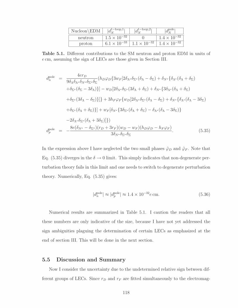
Nucleon\EDM |d1−loop,1N | |d1−loop,2
N | |dpoleN |
neutron 1.5 × 10⁻³² 0 1.4 × 10⁻³²
proton 6.1 × 10⁻³³ 1.1 × 10⁻³² 1.4 × 10⁻³²
Table 5.1. Different contributions to the SM neutron and proton EDM in units ofe cm, assuming the sign of LECs are those given in Section III.
dpolen =
4erD
9δΛδΛ∗δN∗δΣ∗δΣ(hDϕD3wF [2δΛ∗δΣ∗(δΛ − δΣ) + δN∗δΛ∗(δΛ + δΣ)
+δΣ∗(δΣ − 3δΛ)] − wD[2δΛ∗δΣ∗(3δΛ + δΣ) + δN∗3δΛ∗(δΛ + δΣ)
+δΣ∗(3δΛ − δΣ)] + 3hFϕFwD[2δΛ∗δΣ∗(δΛ − δΣ) + δN∗δΛ∗(δΛ − 3δΣ)
+δΣ∗(δΛ + δΣ)] + wF [δN∗3δΣ∗(δΛ + δΣ) − δΛ∗(δΛ − 3δΣ)
−2δΛ∗δΣ∗(δΛ + 3δΣ)])
dpolep = −8e(δN∗ − δΣ∗)(rD + 3rF )(wD − wF )(hDϕD − hFϕF )
3δN∗δΣ∗δΣ. (5.35)
In the expression above I have neglected the two small phases ϕD and ϕF . Note that
Eq. (5.35) diverges in the δ → 0 limit. This simply indicates that non-degenerate per-
turbation theory fails in this limit and one needs to switch to degenerate perturbation
theory. Numerically, Eq. (5.35) gives:
|dpolen | ≈ |dpole
p | ≈ 1.4 × 10⁻³²e cm. (5.36)
Numerical results are summarized in Table 5.1. I caution the readers that all
these numbers are only indicative of the size, because I have not yet addressed the
sign ambiguities plaguing the determination of certain LECs as emphasized at the
end of section III. This will be done in the next section.
5.5 Discussion and Summary
Now I consider the uncertainty due to the undetermined relative sign between dif-
ferent groups of LECs. Since rD and rF are fitted simultaneously to the electromag-
118
netic decay of (1/2)− resonance they should be multiplied by a common undetermined
sign factor δr = ±1. The constant g8 is fitted to the kaon decay rate, so it should carry
a separate sign factor δg. Its phase ϕ however is determined theoretically so it does not
have a sign ambiguity. The four remaining interaction strengths hD, hF , wD, wF are
fitted simultaneously to s and p-wave amplitudes of the hyperon non-leptonic decay,
so they should carry a common undetermined sign factor δhw. Their corresponding
phases are determined by first calculating Imhi exp iϕi and Imwi exp iϕi theoret-
ically and then by dividing them by the experimentally-determined hi, wi so the
four remaining phases ϕD, ϕF , ϕD, ϕF should also carry the same sign factor δhw.
Summing up loop and pole diagram contributions and allowing δr, δg, δhw to freely
change between 1 and -1, I obtain a range of possible dn and dp:
8.7 × 10⁻³⁴e cm < |dn| < 2.8 × 10⁻³²e cm
3.3 × 10⁻³³e cm < |dp| < 3.3 × 10⁻³²e cm (5.37)
The surprisingly small lower bounds of |dn|, |dp| are due to an accidental cancela-
tion between loop and pole-diagram contributions for a very specific set of δi. There
is no reason to believe that this cancellation persists at higher order. To estimate
the size of higher-order contributions, I recall that the HB-expansion parameter is of
order mK/mN ∼ 0.5. Therefore to be conservative, I could assign a 100% error due
to the next-to-leading-order (NLO) effects in the HB-expansion. Also, by looking at
Table 5.1 one can see that both loop and pole diagrams are of order 10−32e cm. So if
I assume no fine cancellation between these two parts after adding the NLO contri-
butions from the HB-expansion, then I should expect the long-distance contribution
to the nucleon EDM to lie within the range:
1 × 10⁻³²e cm < |dn|, |dp| < 6 × 10⁻³²e cm. (5.38)
119
My estimated upper bound for dn is about half the corresponding value predicted
in [161]. Eq. (5.38) is three (four) orders of magnitude smaller than the proposed
precision level of the future proton (neutron) EDM experiments.
To summarize, even though it is well-known that the nucleon EDM induced by
the Standard Model CKM matrix is well below the limit of our current experimental
precision, it is still worth a thorough study as it is currently the only source of intrinsic
EDMs in nature whose existence is certain. I re-analyze previous works on chiral loop
and pole diagram contributions to the nucleon EDM using HBchPT at the leading
order in HB-expansion, with an up-to-date determination of relevant LECs that enter
our calculation. Combined with the uncertainty due to unknown relative signs of
LECs and an estimate of higher-order contributions, I obtain the range for the long-
distance contribution to the nucleon EDM in Eq. (5.38). Although an incalculable
short-distance physics which appears as counterterms in our work could be as large
as the long-distance contribution, the study of the long-distance contribution is still
worthwhile as it provides a safe borderline below which any nucleon EDM is consistent
with the SM prediction. Finally, there are several ways to improve upon the estimate
carried out in this work. For instance, a combined analysis of lattice simulations and
better experimental measurements of various hadronic decay processes is expected to
provide a better control of both the magnitudes and signs of the required LECs. If the
LECs could be determined more precisely, then a complete analysis of NLO-effects in
the HB-expansion would be much desired to further restrict the allowed range of dn
and dp.
120
CHAPTER 6
HIGHER-TWIST CORRECTION TO PVDIS AND ITS
RELATION TO THE PARTON ANGULAR MOMENTUM
6.1 Introduction
As a complement to the studies at high-energy frontier, measurements at the in-
tensity frontier (or precision frontier) provide powerful tools in the search for physics
Beyond the Standard Model (BSM). Observables such as the muon anomalous mag-
netic moment are measured to very high precision, and experimental results are then
compared with theoretical predictions. To the extent that the latter are sufficiently
reliable, any possible deviation would point to BSM physics. Alternately, these ex-
periments can provide new insights into the dynamics of the Standard Model.
Electron-deuteron parity violating deep inelastic scattering (eD PVDIS) is an ex-
cellent example of this class of studies. Historically, it provided the first experimental
measurement of weak mixing angle θW [19]. Nowadays, with the prospect of the Jef-
ferson Laboratory 12-GeV upgrade and the use of a new spectrometer called SoLID,
the left-right asymmetry of PVDIS can be measured with 0.5% precision over the
kinematic range 0.3 < xB < 0.7 [46]. With this level of precision, one will be able
to probe or constrain an interesting set of BSM scenarios, such as a leptophobic Z’
boson[116, 117] and supersymmetry[118], as well as to study hadronic physics effects
which are yet to be fully understood, such as charge symmetry violation (CVC) and
higher-twist (HT).
0Reprinted article with permission from C. Y. Seng and M. J. Ramsey-Musolf, Phys. Rev.C 88 (2013) no.1, 015202. Copyright (2013) by the American Physical Society. DOI:http://dx.doi.org/10.1103/PhysRevC.88.015202
121
The effect of HT [119] is a potentially important Standard Model correction that
originates from the interaction between partons. This correction in general scales
as (Q2)−(τ−2)/2, with the twist τ > 2, so its effect is enhanced at low Q2. In the
framework of the operator product expansion (OPE), the higher-twist correction can
be expressed as a convolution of a high-energy and low-energy piece; the former
(embodied in the Wilson coefficients) can be calculated using perturbative methods,
whereas the latter involves hadronic matrix elements that require understanding of
non-perturbative QCD. Studying the higher-twist correction may help us in prob-
ing correlations between the confined quarks and gluons inside the nucleon, so it is
interesting to explore HT matrix elements within various model approaches. One
advantage of eD PVDIS process is that the HT contribution to the leading term in
the PV asymmetry (defined below) arises from a single operator matrix element and
can, in principle, be separated kinematically from the subleading terms that have
a more complicated HT structure. With this motivation in mind, several previous
works [120, 47, 48, 121] have been carried out to study the twist-four (i.e. τ = 4)
correction to the left-right asymmetry of eD PVDIS. In what follows, we report on a
study that follows-up these earlier works.
The study of HT may also shed light on another important issue, namely, the
spin structure of the nucleon. Nearly twenty-five years ago, the EMC collaboration
[128] performed a DIS experiment with longitudinally-polarized muons on a target of
longitudinally-polarized protons, obtaining a value for the structure function g1(xB)
over the range 0.01 < xB < 0.7. After extrapolating to the low- and high-xB region,
the collaboration obtained a value for the leading moment of g1(xB) that contradicted
the Ellis-Jaffe sum rule [129] and implied that that the spin of proton is not built up
entirely from the quark spin. The result has been confirmed by a variety of subsequent
studies. A key question in nuclear physics research has, thus, become explaining in
detail the source of nucleon spin in terms of QCD degrees of freedom.
122
From a theoretical perspective, arriving at a decomposition of the nucleon spin
in terms of gauge-invariant matrix elements of local operators that afford a straight-
forward partonic interpretation has been a vexing problem, and different approaches
have been pursued over the years[123, 124, 125, 126, 127]. In each case, reference is
usually made to the interpretation in the light-cone – gauge dependence notwithstand-
ing – given its historical importance for thinking about parton dynamics. However,
while the meaning of the quark helicity is gauge invariant, the relative importance
of other aspects of partonic angular momentum (gluon helicity and quark and gluon
orbital angular momentum) in general vary with the choice of gauge and even def-
inition. Nonetheless, it is interesting to ask how different observables may probe
different aspects of partonic angular momentum and to do so in a way that is both
gauge-invariant and as insensitive as possible to a particular angular momentum de-
composition.
In this respect, we will study HT in the context of light-cone quantization. In
early work within this framework, it has been shown that one particular component
of parton angular momentum – identified as quark orbital angular momentum (OAM)
under light-cone quantization using light-cone gauge – is responsible for the non-zero
value of Sivers function and Boer-Mulders function [130, 131] in semi-inclusive deep
inelastic scattering (SIDIS) [132]. In light of these results, it is also interesting to study
how the inclusion of the same component of parton angular momentum modifies the
current model predictions for HT corrections to eD PVDIS. Indeed, in all the previous
studies of eD PVDIS, only the Fock component of the nucleon wavefunction with zero
parton OAM has been included.
After including quark OAM in the light-cone amplitudes, we observe a rather
non-intuitive phenomenon: although the absolute magnitude of individual non-zero
quark OAM contributions can be significant, they largely cancel against each other.
We will argue that this cancelation is largely independent of the detailed model for
123
the relevant light-cone amplitudes. As a result, the twist-four correction to PVDIS
is almost transparent to the inclusion of quark OAM. In contrast, other hadronic
quantities, such as the parton distribution functions (PDF), Sivers function, and
Boer-Mulders function, manifest non-negligible dependence on quark OAM. Gener-
alizing from the particular choice of light-cone quantization and light-cone gauge, we
thus conclude that whatever features of parton angular momentum are responsible for
the observed behavior of the PDFs, Sivers, and Boer-Mulders functions, they should
have a relatively minor impact on the HT correction to eD PVDIS of interest here.
Moreover, any deviation from the light-cone predictions obtained here and in previ-
ous works[120, 47, 48] – should they be observed expermentally – would signal the
importance of other aspects of parton angular momentum and/or higher Fock space
components of the nucleon wavefunction.
The discussion of the computation leading to these observations is arranged in
the following order: in Section II we summarize the relevant results of the general
formulation of the twist-four correction to eD PVDIS; in Section III we introduce the
light-cone wavefunction with quark OAM-dependence; in Section IV we present the
analytic expressions of the hadronic matrix elements needed for the twist-4 correction,
and demonstrate the generic cancelation between non-zero quark OAM components;
in Section V we present the numerical results using one specific choice of nucleon
wavefunction, and discuss their physical significance. Detailed formulae appear in
the Appendix.
6.2 Higher-twist in PVDIS: general formulation
Here, we review the well-known results for the twist-four correction in eD PVDIS.
We will simply quote the central equations that are relevant to our study without
any derivation and refer the reader to Refs. [47, 48] for the details.
124
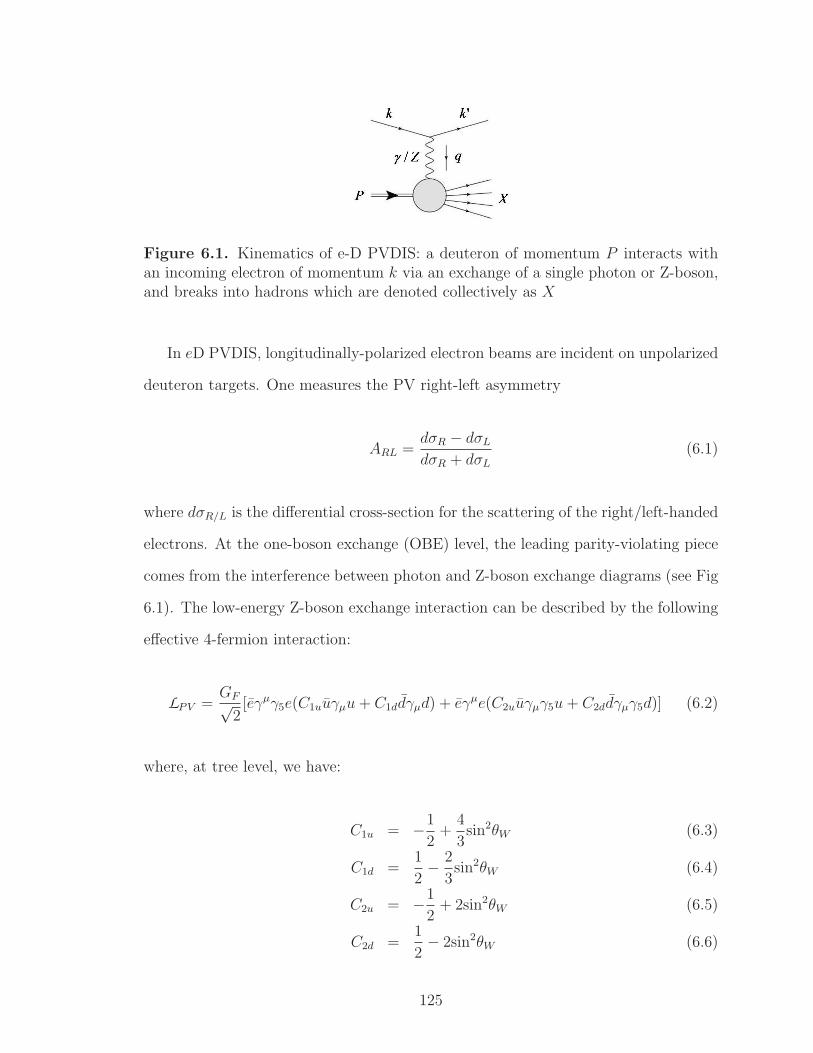
Figure 6.1. Kinematics of e-D PVDIS: a deuteron of momentum P interacts withan incoming electron of momentum k via an exchange of a single photon or Z-boson,and breaks into hadrons which are denoted collectively as X
In eD PVDIS, longitudinally-polarized electron beams are incident on unpolarized
deuteron targets. One measures the PV right-left asymmetry
ARL =dσR − dσL
dσR + dσL
(6.1)
where dσR/L is the differential cross-section for the scattering of the right/left-handed
electrons. At the one-boson exchange (OBE) level, the leading parity-violating piece
comes from the interference between photon and Z-boson exchange diagrams (see Fig
6.1). The low-energy Z-boson exchange interaction can be described by the following
effective 4-fermion interaction:
LPV =GF√
2[eγµγ5e(C1uuγµu+ C1ddγµd) + eγµe(C2uuγµγ5u+ C2ddγµγ5d)] (6.2)
where, at tree level, we have:
C1u = −1
2+
4
3sin2θW (6.3)
C1d =1
2− 2
3sin2θW (6.4)
C2u = −1
2+ 2sin2θW (6.5)
C2d =1
2− 2sin2θW (6.6)
125
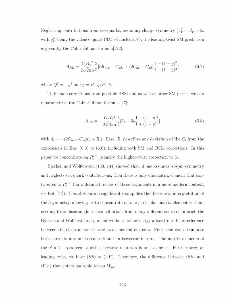
Neglecting contributions from sea quarks, assuming charge symmetry (upV = dn
V , etc.
with qNV being the valence quark PDF of nucleon N), the leading-twist SM prediction
is given by the Cahn-Gilman formula[122]:
ARL =GFQ
2
2√
2πα
3
5[(2C1u − C1d) + (2C2u − C2d)
1 − (1 − y)2
1 + (1 − y)2] (6.7)
where Q2 = −q2 and y = P · q/P · k.
To include corrections from possible BSM and as well as other SM pieces, we can
reparametrize the Cahn-Gilman formula [47]:
ARL = − GFQ2
2√
2πα
3
5[a1 + a2
1 − (1 − y)2
1 + (1 − y)2] (6.8)
with ai = −(2Ciu −Cid)(1 +Ri). Here, Ri describes any deviation of the Ci from the
expressions in Eqs. (6.3) to (6.6), including both SM and BSM corrections. In this
paper we concentrate on RHT1 , namely the higher-twist correction to a1.
Bjorken and Wolfenstein [133, 134] showed that, if one assumes isospin symmetry
and neglects sea quark contributions, then there is only one matrix element that con-
tributes to RHT1 (for a detailed review of these arguments in a more modern context,
see Ref. [47]). This observation significantly simplifies the theoretical interpretation of
the asymmetry, allowing us to concentrate on one particular matrix element without
needing to to disentangle the contributions from many different sources. In brief, the
Bjorken and Wolfenstein argument works as follows: ARL arises from the interference
between the electromagnetic and weak neutral currents. First, one can decompose
both currents into an isoscalar S and an isovector V term. The matrix elements of
the S × V cross-term vanishes because deuteron is an isosinglet. Furthermore, at
leading twist, we have 〈SS〉 = 〈V V 〉. Therefore, the difference between 〈SS〉 and
〈V V 〉 that enters hadronic tensor Wµν
126
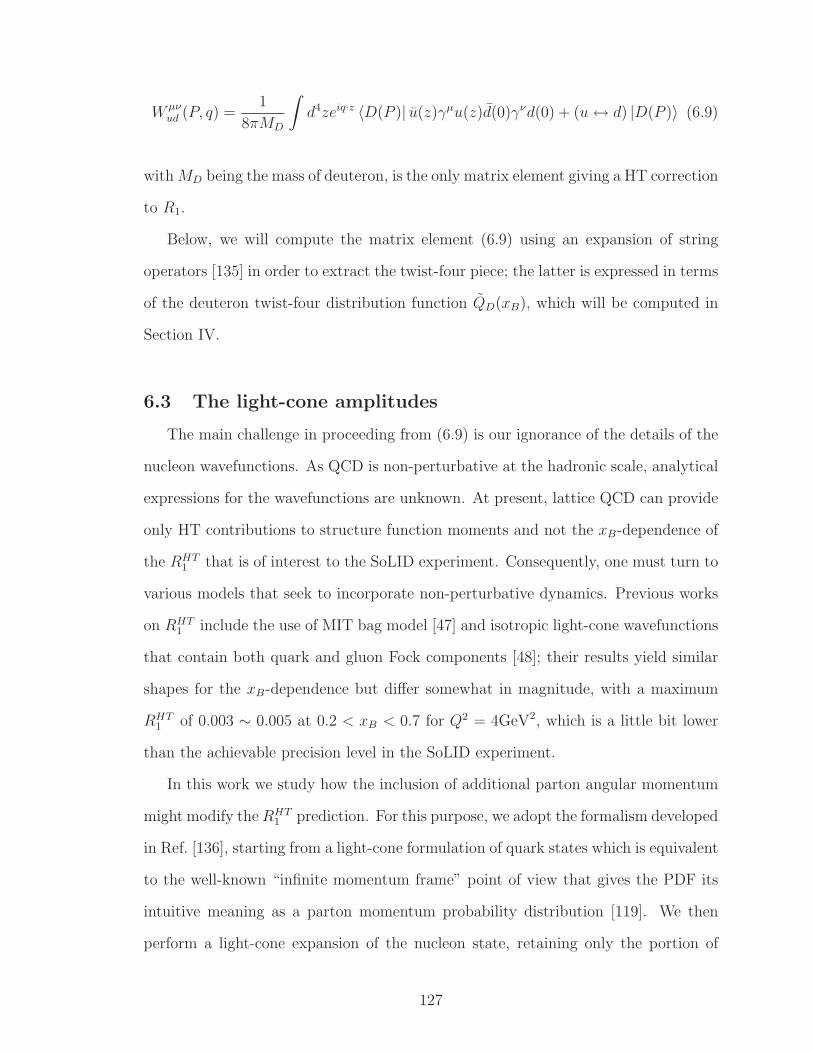
W µνud (P, q) =
1
8πMD
∫
d4zeiq·z 〈D(P )| u(z)γµu(z)d(0)γνd(0) + (u↔ d) |D(P )〉 (6.9)
withMD being the mass of deuteron, is the only matrix element giving a HT correction
to R1.
Below, we will compute the matrix element (6.9) using an expansion of string
operators [135] in order to extract the twist-four piece; the latter is expressed in terms
of the deuteron twist-four distribution function QD(xB), which will be computed in
Section IV.
6.3 The light-cone amplitudes
The main challenge in proceeding from (6.9) is our ignorance of the details of the
nucleon wavefunctions. As QCD is non-perturbative at the hadronic scale, analytical
expressions for the wavefunctions are unknown. At present, lattice QCD can provide
only HT contributions to structure function moments and not the xB-dependence of
the RHT1 that is of interest to the SoLID experiment. Consequently, one must turn to
various models that seek to incorporate non-perturbative dynamics. Previous works
on RHT1 include the use of MIT bag model [47] and isotropic light-cone wavefunctions
that contain both quark and gluon Fock components [48]; their results yield similar
shapes for the xB-dependence but differ somewhat in magnitude, with a maximum
RHT1 of 0.003 ∼ 0.005 at 0.2 < xB < 0.7 for Q2 = 4GeV2, which is a little bit lower
than the achievable precision level in the SoLID experiment.
In this work we study how the inclusion of additional parton angular momentum
might modify theRHT1 prediction. For this purpose, we adopt the formalism developed
in Ref. [136], starting from a light-cone formulation of quark states which is equivalent
to the well-known “infinite momentum frame” point of view that gives the PDF its
intuitive meaning as a parton momentum probability distribution [119]. We then
perform a light-cone expansion of the nucleon state, retaining only the portion of
127
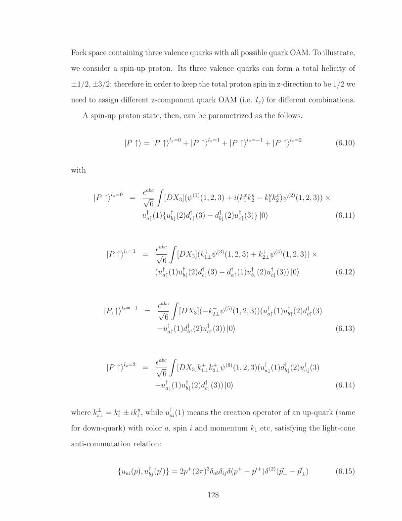
Fock space containing three valence quarks with all possible quark OAM. To illustrate,
we consider a spin-up proton. Its three valence quarks can form a total helicity of
±1/2,±3/2; therefore in order to keep the total proton spin in z-direction to be 1/2 we
need to assign different z-component quark OAM (i.e. lz) for different combinations.
A spin-up proton state, then, can be parametrized as the follows:
|P ↑〉 = |P ↑〉lz=0 + |P ↑〉lz=1 + |P ↑〉lz=−1 + |P ↑〉lz=2 (6.10)
with
|P ↑〉lz=0 =ǫabc
√6
∫
[DX3](ψ(1)(1, 2, 3) + i(kx
1ky2 − ky
1kx2 )ψ(2)(1, 2, 3)) ×
u†a↑(1)u†b↓(2)d†c↑(3) − d†b↓(2)u†c↑(3) |0〉 (6.11)
|P ↑〉lz=1 =ǫabc
√6
∫
[DX3](k+1⊥ψ
(3)(1, 2, 3) + k+2⊥ψ
(4)(1, 2, 3)) ×
(u†a↑(1)u†b↓(2)d†c↓(3) − d†a↑(1)u†b↓(2)u†c↓(3)) |0〉 (6.12)
|P, ↑〉lz=−1 =ǫabc
√6
∫
[DX3](−k−2⊥ψ(5)(1, 2, 3))(u†a↑(1)u†b↑(2)d†c↑(3)
−u†a↑(1)d†b↑(2)u†c↑(3)) |0〉 (6.13)
|P ↑〉lz=2 =ǫabc
√6
∫
[DX3]k+1⊥k
+3⊥ψ
(6)(1, 2, 3)(u†a↓(1)d†b↓(2)u†c↓(3)
−u†a↓(1)u†b↓(2)d†c↓(3)) |0〉 (6.14)
where k±i⊥ = kxi ± iky
i , while u†ai(1) means the creation operator of an up-quark (same
for down-quark) with color a, spin i and momentum k1 etc, satisfying the light-cone
anti-commutation relation:
uai(p), u†bj(p
′) = 2p+(2π)3δabδijδ(p+ − p′+)δ(2)(~p⊥ − ~p′⊥) (6.15)
128
The integration measure is 1:
∫
[DX3] =√
2dx1dx2dx3√2x12x22x3
d2~k1⊥d2~k2⊥d
2~k3⊥(2π)9
2πδ(1 − x1 − x2 − x3) ×
(2π)2δ(2)(~k1⊥ + ~k2⊥ + ~k3⊥) (6.16)
The proton wavefunction amplitudes ψ(1)...ψ(6) are generally unknown functions.
Although the expansion (6.11)∼(6.14) is generic, the explicit form of ψ(i) is model-
dependent. In this work, we chose the form of ψ(i) derived in Ref. [130] by starting
from the static solution of a constituent quark model [137] (which works well in
predicting many electroweak properties of the baryons) and applying a Melosh rota-
tion to the solution to obtain non-zero lz components [138]. This choice of proton
wavefunction is used to predict the first moment of Sivers function, and turns out to
agree fairly well with the experimental measurements from HERMES and COMPASS
[139]2.
6.4 Matrix elements between nucleon states
Following [135], in order to obtain the twist-four distribution function QD(x) we
need to evaluate the matrix elements between state |D(P )〉 of the following operators:
QA(b, z) ≡ : u(b1z)taz/γ5u(b2z)d(b3z)t
az/γ5d(b4z) :
QV (b, z) ≡ : u(b1z)taz/u(b2z)d(b3z)t
az/d(b4z) : (6.17)
where z is a coordinate on light cone, and the parameters b ≡ b1, b2, b3, b4 charac-
terize the light-cone separation between quark field operators.
1There might be difference in constant factors in the definition of integration measure by differentauthors, which only affects the overall normalization.
2Ref. [130] and Ref. [139] defined their first moment of Sivers function with a sign difference.
129
When computing the matrix elements of QV,A in Eq. (6.17) we assume an inco-
herent impulse approximation in which the incoming photon strikes only one of the
two nucleons (see, e.g. Ref. [145] for further discussions regarding the impulse ap-
proximation); hence, matrix elements of the operators (6.17) can be related to the
same matrix elements taken between proton states (or equivalently between neutron
states, given isospin symmetry). Also, since the quantities we compute do not depend
on the proton spin, we can take it to be +1/2 along the z-direction without loss of
generality.
Now, starting from the operators (6.17), we define two distribution functions
Q±(xξ) via
〈P (p) ↑| QV (b, z) ±QA(b, z) |P (p) ↑〉
≡ (p · z)2
∫ 4∏
k=1
dxξkδ(∑
i
xξi)e−i(p·z)
P
k bkxξkQ±(xξ) (6.18)
with xξ collectively representing xξ1 , xξ2 , xξ3 , xξ4, the light-cone momentum frac-
tions: ξ+i = xξi
p+. Meanwhile |P (p) ↑〉 is the spin-up proton state with momentum
p. Substituting (6.11)∼(6.14) into (6.18) we are able to express Q±(xξ) in terms of
the proton wavefunction amplitudes. It is easy to observe that only diagonal terms,
(i.e. terms with the same lz in initial and final states), could give non-vanishing
contributions. After a rather lengthy derivation with the aid of Eq. (H.2), we obtain:
Q±(xξ) = −32π3
3
∫
d2~ξ1⊥(2π)3
...d2~ξ4⊥(2π)3
θ(−xξ1)θ(xξ2)θ(−xξ3)θ(xξ4)θ(1 − xξ2 − xξ4) ×
δ2(~ξ1⊥ + ~ξ2⊥ + ~ξ3⊥ + ~ξ4⊥)∑
lz
ψ±lz(−ξ1,−ξ3, ξ2, ξ4) (6.19)
where the explicit formulas of ψ±lz
are given in Appendix I.
The proton twist-four distribution function can now be expressed in terms of the
Q± (refer to Eq. (42) of Ref. [48] after some rearrangement):
130
Qp(xB) ≡ 2Re
∫ 1
−1
∏4k=1 dxξk
xξ2xξ3(xξ2 + xξ3)δ(∑
k
xξk)(xξ2 + xξ3)δ(xB + xξ1 + xξ2)
−xξ3δ(xB + xξ1) − xξ2δ(xξ4 − xB)[(1 + P14P23)Q+(xξ)
−(P12 + P34)Q−(xξ)] (6.20)
Here Pij is the permutation operator, e.g.
P12Q+(xξ1 , xξ2 , xξ3 , xξ4) = Q+(xξ2 , xξ1 , xξ3 , xξ4). (6.21)
The deuteron twist-four distribution function QD(xB) can be expressed in terms of
Qp(xB) through an incoherent impulse approximation [140], which says that a general
deuteron hadronic tensor can be related to the corresponding hadronic tensors of
proton and neutron by:
MDWµνD (p, q) ≈MNW
µνp (
p
2, q) +MNW
µνn (
p
2, q) (6.22)
where MN is the mass of nucleon. In the equation above each hadronic tensor is
multiplied by the particle’s mass, because following Eq. (6.9) the hadronic tensor
we defined has dimension -1. Now we can express both sides of Eq. (6.22) in terms
of dimensionless structure functions Fi(xB). Using isospin symmetry and the fact
that Q(xB) is proportional to x−1B F ud
1 (xB) (see Eq. (34) of Ref. [48]), we obtain 3:
1
2QD(xB/2) ≈ Qp(xB) + Qn(xB) ≈ 2Qp(xB) (6.23)
Finally, following the logic of Ref. [48], one can the derive the twist-four contri-
bution to R1:
3In Ref. [48], the authors did not multiply their hadronic tensors by particle mass in the impulseapproximation formula, therefore the corresponding relation they obtained is off by a factor 1/2;same for the relation of quark distribution functions.
131
RHT1 (xB, Q
2) =1
Q2
αsπ
5(1 − 209sin2θW )
xBQD(xB)
uD(xB) + dD(xB)(6.24)
with qD(xB) being the parton distribution function for quark of flavor q in the
deuteron
〈D(P )| q(z)z/q(−z) |D(P )〉 = 2(P · z)∫ 1
−1
dxe2i(P ·z)xqD(x) (6.25)
Note that we neglect the logarithmic Q2-dependence of the structure functions in this
analysis. We can express qD in terms of PDF of the proton and neutron again by the
impulse approximation (6.22), but now comparing the structure function F2(xB) on
both sides, which is proportional to x−1B q(xB). The result is:
qD(xB/2) ≈ qp(xB) + qn(xB) (6.26)
where qp(x) and qn(x) are defined as in Eq. (6.25) but for proton/neutron states.
Furthermore, neglecting CSV effects we have:
un(xB) = dp(xB), dn(xB) = up(xB) (6.27)
Therefore, it is sufficient to just calculate up(xB) and dp(xB) using the proton light-
cone wavefunction (6.11)∼(6.14). Using (H.3) and (H.4) , we can compute the quark
PDFs of the (spin-up) nucleons by calculating the matrix element on LHS of Eq.
(6.25) with nucleon states, and compare it with the form on RHS to extract the
PDFs. Same with the twist-four distribution functions, only terms diagonal to lz
survive, so we can separate the result into components of different lz as the following:
up(xB) + dp(xB) = dn(xB) + un(xB)
=1
(2π)6
∫ 1
0
dx1
∫
d2~k1⊥d2~q⊥Θ(1 − xB − x1)
∑
lz
Alz(q, 1, 2)
(6.28)
132
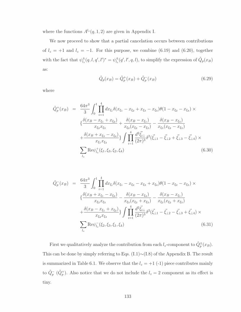
where the functions Alz(q, 1, 2) are given in Appendix I.
We now proceed to show that a partial cancelation occurs between contributions
of lz = +1 and lz = −1. For this purpose, we combine (6.19) and (6.20), together
with the fact that ψ±lz(q, l, q′, l′)∗ = ψ±
lz(q′, l′, q, l), to simplify the expression of Qp(xB)
as:
Qp(xB) = Q+p (xB) + Q−
p (xB) (6.29)
where
Q+p (xB) =
64π3
3
∫ 1
0
4∏
i=1
dxξiδ(xξ1 − xξ2 + xξ3 − xξ4)θ(1 − xξ2 − xξ4) ×
δ(xB − xξ1 + xξ2)
xξ2xξ3
+δ(xB − xξ1)
xξ2(xξ2 − xξ3)− δ(xB − xξ4)
xξ3(xξ2 − xξ3)
+δ(xB + xξ3 − xξ4)
xξ1xξ4
∫ 4∏
i=1
d2~ξi⊥(2π)3
δ2(~ξ⊥1 − ~ξ⊥2 + ~ξ⊥3 − ~ξ⊥4) ×∑
lz
Reψ+lz(ξ1, ξ3, ξ2, ξ4) (6.30)
Q−p (xB) =
64π3
3
∫ 1
0
4∏
i=1
dxξiδ(xξ1 − xξ2 − xξ3 + xξ4)θ(1 − xξ2 − xξ3) ×
δ(xB + xξ1 − xξ2)
xξ2xξ3
− δ(xB − xξ4)
xξ3(xξ2 + xξ3)− δ(xB − xξ1)
xξ2(xξ2 + xξ3)
+δ(xB − xξ1 + xξ2)
xξ2xξ3
∫ 4∏
i=1
d2~ξi⊥(2π)3
δ2(~ξ⊥1 − ~ξ⊥2 − ~ξ⊥3 + ~ξ⊥4) ×∑
lz
Reψ−lz(ξ2, ξ3, ξ1, ξ4) (6.31)
First we qualitatively analyze the contribution from each lz-component to Q±p (xB).
This can be done by simply referring to Eqs. (I.1)∼(I.8) of the Appendix B. The result
is summarized in Table 6.1. We observe that the lz = +1 (-1) piece contributes mainly
to Q−p (Q+
p ). Also notice that we do not include the lz = 2 component as its effect is
tiny.
133
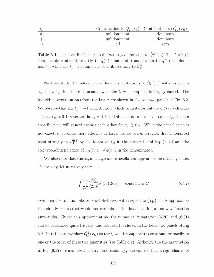
lz Contribution to Q+p (xB) Contribution to Q−
p (xB)
0 subdominant dominant+1 subdominant dominant-1 all zero
Table 6.1. The contributions from different lz-components to Q±p (xB). The lz=0,+1
components contribute mostly to Q−p (“dominant”) and less so to Q+
p (“subdomi-
nant”), while the lz=-1 component contributes only to Q+p .
Next we study the behavior of different contributions to Q±p (xB) with respect to
xB, showing that those associated with the lz ± 1 components largely cancel. The
individual contributions from the latter are shown in the top two panels of Fig. 6.2.
We observe that the lz = −1 contribution, which contributes only to Q+p (xB) changes
sign at xB ≈ 0.4, whereas the lz = +1 contribution does not. Consequently, the two
contributions will cancel against each other for xB>∼ 0.4. While the cancellation is
not exact, it becomes more effective at larger values of xB, a region that is weighted
most strongly in RHT1 by the factor of xB in the numerator of Eq. (6.24) and the
corresponding presence of uD(xB) + dD(xB) in the denominator.
We also note that this sign change and cancellation appears to be rather generic.
To see why, let us naively take:
∫ 4∏
i=1
d2~ξi⊥(2π)3
δ2(...)Reψ±lz≈ constant ≡ C (6.32)
assuming the function above is well-behaved with respect to xξi. This approxima-
tion simply means that we do not care about the details of the proton wavefunction
amplitudes. Under this approximation, the numerical integration (6.30) and (6.31)
can be performed quite trivially, and the result is shown in the lower two panels of Fig
6.2. In this case, we show Q±p (xB) as the lz = ±1 components contribute primarily to
one or the other of these two quantities (see Table 6.1). Although the the assumption
in Eq. (6.32) breaks down at large and small xB, one can see that a sign change of
134
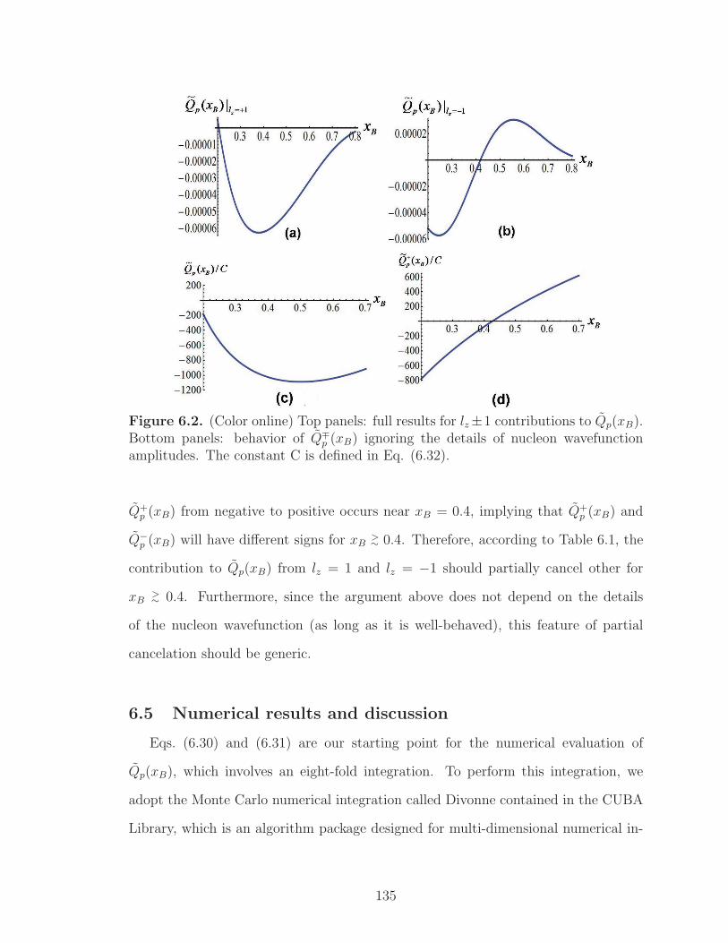
Figure 6.2. (Color online) Top panels: full results for lz±1 contributions to Qp(xB).Bottom panels: behavior of Q∓
p (xB) ignoring the details of nucleon wavefunctionamplitudes. The constant C is defined in Eq. (6.32).
Q+p (xB) from negative to positive occurs near xB = 0.4, implying that Q+
p (xB) and
Q−p (xB) will have different signs for xB
>∼ 0.4. Therefore, according to Table 6.1, the
contribution to Qp(xB) from lz = 1 and lz = −1 should partially cancel other for
xB>∼ 0.4. Furthermore, since the argument above does not depend on the details
of the nucleon wavefunction (as long as it is well-behaved), this feature of partial
cancelation should be generic.
6.5 Numerical results and discussion
Eqs. (6.30) and (6.31) are our starting point for the numerical evaluation of
Qp(xB), which involves an eight-fold integration. To perform this integration, we
adopt the Monte Carlo numerical integration called Divonne contained in the CUBA
Library, which is an algorithm package designed for multi-dimensional numerical in-
135
Figure 6.3. (Color online)The Twist-4 correction to R1 at Q2 = 4GeV2. The bluedashed curve shows the lz = 0 contribution; purple dot-dashed curve shows the lz = 1contribution; brown dot-dashed curve shows the lz = −1 contribution; the red solidcurve is the sum of all. lz = 2 contribution is negligible and therefore not included.
tegration [141]. For each lz component, we evaluate the value of Qp(xB) at a series
of discrete xB,i, and then link them together using a best-fit line. Also, we take
αs = 0.5 at 1GeV following the renormalization group (RG) prediction of the running
coupling constant at 4-loop order together with a 3-loop threshold matching, with the
quark thresholds taken to be Mc = 1.5 GeV and Mb = 4.7 GeV respectively [142].
Our main result is shown in Fig. 6.3, which gives RHT1 versus x′B ≡ 2xB at
Q2 = 4GeV2. First, let us compare this outcome with that of Refs. [47] and [48]. It
turns out that all three calculations predict similar curve shape for RHT1 , only with
slightly different positions of peak and zero-point. Concerning the magnitude, our
work predicts a maximum absolute value |RHT1 | ≈ 2.6×10⁻³ between 0.2 < x′B < 0.7,
which is smallest in magnitude among all the three predictions, and is about a half of
the size to that of Ref. [48]. This is understandable because the authors include a 3-
quark+1-gluon Fock-space component whose contribution is comparable in magnitude
to that of the pure 3-quark state. Nonetheless, all three calculations suggest that
|RHT1 | lies below that of the expected SoLID precision.
Next we study the OAM-dependence in detail. To that end, we first introduce
some nomenclature: in the following, we will use the notation (|lz| ⊗ |lz′ |), which
denotes a generic matrix element taking between two hadronic states, of which one of
136

Figure 6.4. (color online)The unnormalized QDF of spin-up proton, splitted intocontributions from different lz components. Blue thick-dashed curve shows contribu-tion from lz = 0 component; purple dot-dashed curve shows contribution from lz = 1component; brown dot-dashed curve shows contribution from lz = −1 component;green thin-dashed curve shows contribution from lz = 2 component; red solid curveis the sum of all contributions.
them has absolute value of quark OAM in z-direction being |lz| and the other being
|lz′ |.
From our arguments at the end of Section 6.4, we expect that although lz = ±1
individually contribute a significant amount to Qp(xB), they should largely cancel
against each other for xB > 0.4, making the total (1 ⊗ 1) contribution rather small,
and therefore leaving the (0⊗0) contribution as the dominant piece. This expectation
is born out by the curves in Fig. 6.3. The purple dot-dashed curve and brown dot-
dashed curve curves give the individual (lz = 1)⊗ (lz = 1) and (lz = −1)⊗ (lz = −1)
contributions, respectively , which exhibit the expected cancellation for x′B > 0.4.
The blue dashed curve and red solid curve give the (0 ⊗ 0) and total contributions,
respectively. It is clear that the former dominates the total. This (0 ⊗ 0) dominance
is a rather unique feature of the particular twist-four contribution of interest here,
and one that is not shared by other diagonal matrix elements. For example, if one
calculate proton quark PDFs (leading twist) using the same set of wavefunctions, the
(0⊗ 0) and (1⊗ 1) contributions are comparable; moreover, since they have the same
sign, the two |lz| = 1 pieces do not cancel each other (see Fig.6.4).
137
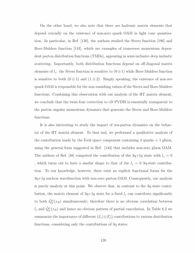
On the other hand, we also note that there are hadronic matrix elements that
depend crucially on the existence of non-zero quark OAM in light cone quantiza-
tion. In particular, in Ref. [130], the authors studied the Sivers function [196] and
Boer-Mulders function [143], which are examples of transverse momentum depen-
dent parton distribution functions (TMDs), appearing in semi-inclusive deep inelastic
scattering. Importantly, both distribution functions depend on off-diagonal matrix
elements of lz: the Sivers function is sensitive to (0⊗ 1) while Boer-Mulders function
is sensitive to both (0 ⊗ 1) and (1 ⊗ 2). Simply speaking, the existence of non-zeo
quark OAM is responsible for the non-vanishing values of the Sivers and Boer-Mulders
functions. Combining this observation with our analysis of the HT matrix element,
we conclude that the twist-four correction to eD PVDIS is essentially transparent to
the parton angular momentum dynamics that generate the Sivers and Boer-Mulders
functions.
It is also interesting to study the impact of sea-parton dynamics on the behav-
ior of the HT matrix element. To that end, we performed a qualitative analysis of
the contribution made by the Fock space component containing 3 quarks + 1 gluon,
using the general form suggested in Ref. [144] that includes non-zero gluon OAM.
The authors of Ref. [48] computed the contribution of the 3q+1g state with lz = 0
, which turns out to have a similar shape to that of the lz = 0 3q-state contribu-
tion. To our knowledge, however, there exist no explicit functional forms for the
3q+1g nucleon wavefunction with non-zero parton OAM. Consequently, our analysis
is purely analytic at this point. We observe that, in contrast to the 3q state contri-
bution, the matrix element of 3q+1g state for a fixed lz can contribute significantly
to both Q±p (xB) simultaneously; therefore there is no obvious correlation between
lz and Q±p (xB) and hence no obvious pattern of partial cancelation. In Table 6.2 we
summarize the importance of different (|lz|⊗|l′z|) contributions to various distribution
functions, considering only the contributions of 3q states.
138
Distribution Functions Dominant SubdominantQuark Distribution Functions (0×0), (1⊗1) (2⊗2)PVDIS Twist-Four Correction (0⊗0) (1⊗1), (2⊗2)
Sivers Function (0⊗1) (1⊗2)Boer-Mulders Function (0⊗1), (1⊗2) —
Table 6.2. The dependence on different quark light-cone OAM components of variousdistribution functions.
Combining observations, we may draw the following conclusion: if a future eD
PVDIS measurement yields a sufficiently precise determination of RHT1 as a function
of x′B, one can compare the experimental curve with our current theoretical prediction.
A significant deviation from the predicted curve (e.g., the peak and zero-point are
shifted by a considerable amount), could signal the importance of parton angular
momentum dynamics beyond those responsible for the Sivers, Boer-Mulders, and
spin-independent parton distribution functions.
6.6 Summary
The next generation of parity-violating electron scattering experiments are poised
to probe both possible BSM physics as well as novel features of hadron and nuclear
structure. In this work, we have studied one particular hadronic effect, namely,
the twist-four contribution to a1, the y-independent term in the PV asymmetry.
Using a set of proton light-cone wavefunctions with non-zero quark orbital angular
momentum, we evaluated the twist-four contribution as a function of xB, identifying
the contributions from different OAM-components. Our total for the correction RHT1
is similar in both shape and magnitude to those obtained in previous works, indicating
that higher-precision than expected with the SoLID experiment would be needed to
discern this HT effect. An effort to achieve such precision may be worthwhile, because
RHT1 appears to be rather unique, in the sense that it is not significantly affected by
the parton angular momentum physics responsible for the existence of some other
139
DIS observables such as the Sivers and Boer-Mulders functions. Thus, by combining
the results of a more precise measurement of the asymmetry with measurements of
other distribution functions, it is possible to probe complementary aspects of parton
angular momentum and, perhaps, shed new light on the role of angular momentum
in the structure of the nucleon.
140

CHAPTER 7
CONCLUSION
There are many open questions in both the SM and BSM physics remained to
be answered. In particular, this thesis focuses mainly on: (1) the understanding of
QCD at low energy and its application in hadrons and nuclear systems, and (2) the
description of effects of new physics through effective field theory and probes of BSM
physics in various low energy experiments, including tests of fundamental symmetries
in hadrons and nuclei. These two areas of research merge naturally as the development
of various effective approaches to the low energy QCD does not only offers a better
understanding of the original theory itself in the non-perturbative regime but also
provides inputs, such as various QCD matrix elements, that are needed to interpret
searches for BSM physics via low energy precision experiments. Throughout this
thesis, I try to address the following questions with several case studies:
1. What are the currently-available effective approaches to hadron physics and
how well can they reproduce behaviors of QCD at low energy,
2. How precisely can we evaluate the relevant QCD matrix elements with our
currently knowledge and computational technique in hadron physics,
3. What are the limitations and deficiencies of each effective approach, and
4. What can we do to improve our current knowledge and computational tech-
niques in the two areas listed above.
In the first two chapters involving the application of Dyson-Schwinger Equation,
the main motivation is to search for a unified formalism that can be used to study
141
the low energy effects of all effective operators in the same footing with a manage-
able amount of theoretical calculation. We show that DSE with an extremely simple
contact interaction approximation is capable to reproduce many known static prop-
erties of hadrons as good as other more sophisticated methods. With this simple
approximation we calculated both the EDM of a ρ-meson induced by several effective
operators up to dimension 6 and various static charges of nucleon.
Upon comparing our result with existing calculations we find that the degree of
agreement with other calculations depends operator-by-operator. This raises a general
question of how one could possibly estimate the degree of accuracy within each model
calculations. Currently there exists no commonly-agreed algorithm for this purpose.
As far as practical usage is concerned, the standard way adopted by the community
is simply to take the spread of calculations performed using different models as the
theoretical error of the calculated quantity. This is obviously not promising enough
because any additional theoretical effort in the future will only increase the amount
of spread and not decrease it. Therefore, we believe that an essential step in the
future is to develop a universal formalism that allows us to quantify the theoretical
calculation within any given model.
In the next three chapters I switch my attention to Chiral Perturbation Theory. I
demonstrate how an effective theory can be built based on very general arguments of
symmetry. This kind of effective theory is sensitive to the IR behavior of QCD. One
of the many unique features of ChPT is the prediction of non-analytical dependence
on quark masses in scattering amplitudes. Besides, the importance of a valid power
counting scheme in non-renormalizable field theories is also stressed in these chapter.
In fact, both the works on g(i)π and SM EDM are basically improvements of existing
literatures using the heavy baryon formalism that respects chiral power counting. In
particular, it is shown in the g(i)π calculation that the loss of valid power counting in
142
ChPT may lead to an overestimation of O(mN/mπ) ∼10 times in the calculation of
low energy observables.
Some obvious deficiencies of ChPT-like effective theories are also clearly revealed
in these two works. The key point is that effective theories constructed merely from
the symmetry considerations contains too many degrees of freedom (in parameters)
compared to the original theory. A direct consequence is that the constructed EFT
then contains infinitely many free parameters undetermined by the theory itself. For
example, UV-divergences in chiral loop integrals must be canceled by counterterms
which appear as higher-order LECs. These counterterms are not a priori known
and what we can do at most without referring to inputs from lattice or other model
calculations is to estimate their order of magnitudes using dimensional analysis. For
the observables studied in Chapter 4 and 5 we find that the size of these counterterms
can be as large as the loop correction so the ignorance of the numerical values of
counterterms renders our theory prediction less useful. Currently the only promising
way to determine these pieces is through fittings in lattice simulation. I believe that
one of the interesting future directions will be to explore alternative methods in the
determination of counterterms involving applications of chiral-improved models.
In Chapter 6 I present an alternative viewpoint to the interplay between low
energy QCD and searches of BSM physics. In this chapter, the key message is not
just that better QCD calculation is needed for the interpretation of experiment, but
the opposite is also true. In this particular example, the twist-four matrix element
which is a relevant SM background in BSM searches through PVDIS could actually
be measured experimentally and it turns out to also teach us interesting features
of QCD, in this case the role of parton angular momentum in the nucleon spin.
Combining with other parton distribution functions measurable in SIDIS, it provides
a possibility for us to perform a systematic study on different components of parton
angular momentum in nucleon separately.
143
As a conclusion, we are still very far away from having a satisfactory effective
description of hadrons that is universal, theoretically clean and computationally eco-
nomical. With particular working examples, I give a flavor of how much one can do
using current available effective approaches in terms of calculations of relevant QCD
matrix elements that play key roles in the low-energy tests of fundamental symme-
tries in systems of hadrons and point out several possible directions one may improve
from. It will be a true excitement if any of us here can live long enough to witness
a fundamental breakthrough either in the understanding of QCD at hadronic scale
or the search of BSM physics as either of them could easily be listed as one of the
greatest triumphs of mankind since the born of modern physics.
144
APPENDIX A
CONTACT INTERACTION
In this appendix we include some detail of the contact interaction approximation
we used to describe the low-energy interaction between quarks in our DSE formalism.
Our treatment of the contact interaction begins with the gap equation
S(p)−1 = iγ · p+m
+
∫
d4q
(2π)4g2Dµν(p− q)
λa
2γµS(q)
λa
2Γν(q, p), (A.1)
wherein m is the Lagrangian current-quark mass, Dµν is the vector-boson propagator
and Γν is the quark–vector-boson vertex. We work with the choice
g2Dµν(p− q) = δµν4παIR
m2G
, (A.2)
where mG = 0.8 GeV is a gluon mass-scale typical of the one-loop renormalisation-
group-improved interaction introduced in Ref. [83], and the fitted parameter αIR/π =
0.93 is commensurate with contemporary estimates of the zero-momentum value of a
running-coupling in QCD [93, 94]. Equation (A.2) is embedded in a rainbow-ladder
(RL) truncation of the DSEs, which is the leading-order in the most widely used,
global-symmetry-preserving truncation scheme [76, 77]. This means
Γν(p, q) = γν (A.3)
in Eq. (A.1) and in the subsequent construction of the Bethe-Salpeter kernels.
145
One may view the interaction in Eq. (A.2) as being inspired by models of the
Nambu–Jona-Lasinio type [95]. However, our treatment is atypical. Moreover, as
noted in the Introduction, one normally finds Eqs. (A.2), (A.3) produce results for
low-momentum-transfer observables that are practically indistinguishable from those
produced by more sophisticated interactions [64, 65, 67, 66, 68, 69, 216, 217, 218, 219,
220]. Using Eqs. (A.2), (A.3), the gap equation becomes
S−1(p) = iγ · p+m+16π
3
αIR
m2G
∫
d4q
(2π)4γµ S(q) γµ , (A.4)
an equation in which the integral possesses a quadratic divergence. When the diver-
gence is regularised in a Poincare covariant manner, the solution is
S(p)−1 = iγ · p+M , (A.5)
where M is momentum-independent and determined by
M = m+M4αIR
3πm2G
∫ ∞
0
ds s1
s+M2. (A.6)
We define Eq. (A.4) by writing [96]
1
s+M2=
∫ ∞
0
dτ e−τ(s+M2)
→∫ τ2
ir
τ2uv
dτ e−τ(s+M2) (A.7)
=e−(s+M2)τ2
uv − e−(s+M2)τ2ir
s+M2, (A.8)
where τir,uv are, respectively, infrared and ultraviolet regulators. It is apparent from
Eq. (A.8) that a finite value of τir =: 1/Λir implements confinement by ensuring the
absence of quark production thresholds [97]. Since Eq. (A.2) does not define a renor-
malisable theory, then Λuv := 1/τuv cannot be removed but instead plays a dynamical
146

role, setting the scale of all dimensioned quantities. Using Eq. (A.7), the gap equation
becomes
M = m+M4αIR
3πm2G
C iu(M2) , (A.9)
where,
C iu(ω) = ω [Γ(−1, ωτ 2uv) − Γ(−1, ωτ 2
ir)] , (A.10)
with Γ(α, y) being the incomplete gamma-function.
At this point we also list expressions for the other regularised integrals that we
employ herein:
C iun (ω) = (−1)nω
n
n!
dn
dωnC iu(ω) , (A.11)
D iu(ω) =
∫
R
dss2
s+M2
= 2ω2 [Γ(−2, ωτ 2uv) − Γ(−2, ωτ 2
ir)] , (A.12)
E iu(ω) =
∫
R
dss3
s+M2
= 6ω3 [Γ(−3, ωτ 2uv) − Γ(−3, ωτ 2
ir)] , (A.13)
G iu1 (ω) =
∫
R
dss
(s+ ω)3 =1
2
d2
dω2C iu(ω) , (A.14)
G iu2 (ω) =
∫
R
dss2
(s+ ω)3
= C iu1 (ω) − ω
2
d2
dω2C iu(ω) , (A.15)
G iu3 (ω) =
∫
R
dss3
(s+ ω)3
= C iu(ω) − 2 C iu1 (ω) + C iu
2 (ω) , (A.16)
G iu4 (ω) =
∫
R
dss4
(s+ ω)3 = D iu(ω)
− 2ω C iu(ω) + 3ω C iu1 (ω) − ω C iu
2 (ω) , (A.17)
G iu5 (ω) =
∫
R
dss5
(s+ ω)3 = E iu(ω) − 2ωD iu(ω)
147
+ 3ω2 C iu(ω) − 4ω2 C iu1 (ω) + ω2 C iu
2 (ω) , (A.18)
where Gi = Gi/(16π2), i = 1, . . . , 5.
The parameters that specify our treatment of the contact interaction were de-
termined in a study of π- and ρ-meson properties [66]; viz., αIR/π = 0.93 and (in
GeV)
m = 0.007 , Λir = 0.240 Λuv = 0.905 , (A.19)
using which, Eq. (A.9) yields
M = 0.368 GeV. (A.20)
With the aim of exploring the impact of DCSB on our results, herein we also
consider results obtained with αIR/π = 0.74, in which case
M →M< = 0.246 GeV. (A.21)
148
APPENDIX B
FADDEEV EQUATION
We describe the dressed-quark-cores of the nucleon via solutions of a Poincare-
covariant Faddeev equation [250]. The equation is derived following upon the observa-
tion that an interaction which describes mesons also generates quark-quark (diquark)
correlations in the colour-3 channel [251]. The fidelity of the diquark approximation
to the quark-quark scattering kernel has been verified [91].
In RL truncation, the colour-antitriplet diquark correlations are described by an
homogeneous Bethe-Salpeter equation that is readily inferred from the analogous
meson equation; viz., following Ref. [251] and expressing the diquark amplitude as
Γcqq(k;P ) = Γqq(k;P )C†Hc, (B.1)
with
H1 = iλ7, H2 = −iλ5, H3 = iλ2 , ǫc1c2c3 = (Hc3)c1c2 , (B.2)
where λ2,5,7 are Gell-Mann matrices, then
Γqq(k;P ) = −8π
3
αIR
m2G
∫
d4q
(2π)4γµχqq(q;P )γµ , (B.3)
where χqq(q;P ) = S(q)Γqq(P )S(q − P ) and Γqq is the diquark Bethe-Salpeter ampli-
tude, which is independent of the relative momentum when using a contact interaction
[66].
149
Scalar and axial-vector quark-quark correlations are dominant in studies of the
nucleon:
Γ0+
qq (P ) = iγ5Eqq0(P ) +1
Mγ5γ · PFqq0(P ) , (B.4)
iΓ1+
qq µ(P ) = iγTµEqq1(P ), (B.5)
where PµγTµ = 0. These amplitudes are canonically normalised:
Pµ = 2tr
∫
d4q
(2π)4Γ0+
qq (−P )∂
∂Pµ
S(q + P )Γ0+
qq (P )S(q); (B.6)
and
Pµ =2
3tr
∫
d4q
(2π)4Γ1+
qq α(−P )∂
∂Pµ
S(q + P )Γ1+
qq α(P )S(q). (B.7)
A J = 12
baryon is represented by a Faddeev amplitude
Ψ = Ψ1 + Ψ2 + Ψ3 , (B.8)
where the subscript identifies the bystander quark and, e.g., Ψ1,2 are obtained from
Ψ3 by a cyclic permutation of all the quark labels. We employ a simple but realistic
representation of Ψ. The spin- and isospin-12
nucleon is a sum of scalar and axial-
vector diquark correlations:
Ψ3(pi, αi, τi) = N 0+
3 + N 1+
3 , (B.9)
with (pi, αi, τi) the momentum, spin and isospin labels of the quarks constituting the
bound state, and P = p1 + p2 + p3 the system’s total momentum.
150
The scalar diquark piece in Eq. (B.9) is
N 0+
3 (pi, αi, τi) = [Γ0+
(1
2p[12];K)]τ1τ2
α1α2∆0+
(K) [S(ℓ;P )u(P )]τ3α3, (B.10)
where: the spinor satisfies Eq. (G.4), with M the mass obtained by solving the Fad-
deev equation, and it is also a spinor in isospin space with ϕ+ = col(1, 0) for the
charge-one state and ϕ− = col(0, 1) for the neutral state; K = p1 + p2 =: p12,
p[12] = p1 − p2, ℓ := (−p12 + 2p3)/3;
∆0+
(K) =1
K2 +m2qq
0+
(B.11)
is a propagator for the scalar diquark formed from quarks 1 and 2, with mqq0+
the
mass-scale associated with this correlation, and Γ0+
is the canonically-normalised
Bethe-Salpeter amplitude described above; and S , a 4×4 Dirac matrix, describes the
relative quark-diquark momentum correlation.
The axial-vector component in Eq. (B.9) is
N 1+
(pi, αi, τi) = [ti Γ1+
µ (1
2p[12];K)]τ1τ2
α1α2∆1+
µν (K) [A iν(ℓ;P )u(P )]τ3α3
, (B.12)
where the symmetric isospin-triplet matrices are
t+ =
1√2(τ 0 + τ 3) , t0 = τ 1 , t− =
1√2(τ 0 − τ 3) , (B.13)
and the other elements in Eq. (B.12) are straightforward generalisations of those in
Eq. (B.10) with, e.g.,
∆1+
µν (K) =1
K2 +m2qq
1+
(
δµν +KµKν
m2qq
1+
)
. (B.14)
151
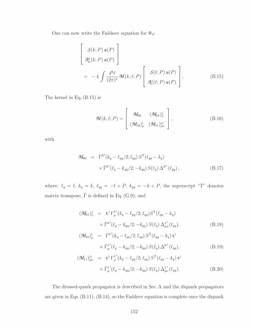
One can now write the Faddeev equation for Ψ3:
S(k;P ) u(P )
A iµ(k;P ) u(P )
= − 4
∫
d4ℓ
(2π)4M (k, ℓ;P )
S(ℓ;P ) u(P )
A jν(ℓ;P ) u(P )
. (B.15)
The kernel in Eq. (B.15) is
M (k, ℓ;P ) =
M00 (M01)jν
(M10)iµ (M11)
ijµν
, (B.16)
with
M00 = Γ0+
(kq − ℓqq/2; ℓqq)ST(ℓqq − kq)
× Γ0+
(ℓq − kqq/2;−kqq)S(ℓq) ∆0+
(ℓqq) , (B.17)
where: ℓq = ℓ, kq = k, ℓqq = −ℓ + P , kqq = −k + P , the superscript “T” denotes
matrix transpose, Γ is defined in Eq. (G.9); and
(M01)jν = t
j Γ1+
µ (kq − ℓqq/2; ℓqq)ST(ℓqq − kq)
× Γ0+
(ℓq − kqq/2;−kqq)S(ℓq) ∆1+
µν (ℓqq), (B.18)
(M10)iµ = Γ0+
(kq − ℓqq/2; ℓqq)ST(ℓqq − kq) t
i
× Γ1+
µ (ℓq − kqq/2;−kqq)S(ℓq) ∆0+
(ℓqq), (B.19)
(M11)ijµν = t
j Γ1+
ρ (kq − ℓqq/2; ℓqq)ST(ℓqq − kq) t
i
× Γ1+
µ (ℓq − kqq/2;−kqq)S(ℓq) ∆1+
ρν (ℓqq). (B.20)
The dressed-quark propagator is described in Sec. A and the diquark propagators
are given in Eqs. (B.11), (B.14), so the Faddeev equation is complete once the diquark
152
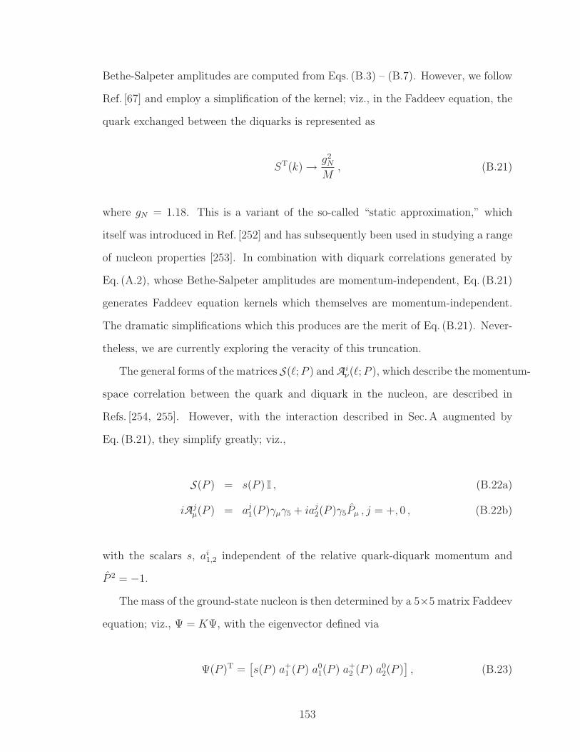
Bethe-Salpeter amplitudes are computed from Eqs. (B.3) – (B.7). However, we follow
Ref. [67] and employ a simplification of the kernel; viz., in the Faddeev equation, the
quark exchanged between the diquarks is represented as
ST(k) → g2N
M, (B.21)
where gN = 1.18. This is a variant of the so-called “static approximation,” which
itself was introduced in Ref. [252] and has subsequently been used in studying a range
of nucleon properties [253]. In combination with diquark correlations generated by
Eq. (A.2), whose Bethe-Salpeter amplitudes are momentum-independent, Eq. (B.21)
generates Faddeev equation kernels which themselves are momentum-independent.
The dramatic simplifications which this produces are the merit of Eq. (B.21). Never-
theless, we are currently exploring the veracity of this truncation.
The general forms of the matrices S(ℓ;P ) and A iν(ℓ;P ), which describe the momentum-
space correlation between the quark and diquark in the nucleon, are described in
Refs. [254, 255]. However, with the interaction described in Sec. A augmented by
Eq. (B.21), they simplify greatly; viz.,
S(P ) = s(P ) I , (B.22a)
iA jµ(P ) = aj
1(P )γµγ5 + iaj2(P )γ5Pµ , j = +, 0 , (B.22b)
with the scalars s, ai1,2 independent of the relative quark-diquark momentum and
P 2 = −1.
The mass of the ground-state nucleon is then determined by a 5×5 matrix Faddeev
equation; viz., Ψ = KΨ, with the eigenvector defined via
Ψ(P )T =[
s(P ) a+1 (P ) a0
1(P ) a+2 (P ) a0
2(P )]
, (B.23)
153
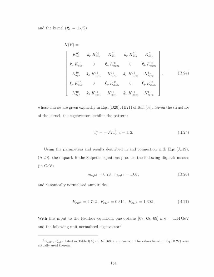
and the kernel (k± = ±√2)
K(P ) =
K00ss k−K
01sa1
K01sa1
k−K01sa2
K01sa2
k−K10a1s 0 k+K
11a1a1
0 k+K11a1a2
K10a1s k+K
11a1a1
K11a1a1
k+K11a1a2
K11a1a2
k−K10a2s 0 k+K
11a2a1
0 k+K11a2a2
K10a2s k+K
11a2a1
K11a2a1
k+K11a2a2
K11a2a2
, (B.24)
whose entries are given explicitly in Eqs. (B20), (B21) of Ref. [68]. Given the structure
of the kernel, the eigenvectors exhibit the pattern:
a+i = −
√2a0
i , i = 1, 2. (B.25)
Using the parameters and results described in and connection with Eqs. (A.19),
(A.20), the diquark Bethe-Salpeter equations produce the following diquark masses
(in GeV)
mqq0+ = 0.78 , mqq1+ = 1.06 , (B.26)
and canonically normalised amplitudes:
Eqq0+ = 2.742 , Fqq0+ = 0.314 , Eqq1+ = 1.302 . (B.27)
With this input to the Faddeev equation, one obtains [67, 68, 69] mN = 1.14 GeV
and the following unit-normalised eigenvector1
1Eqq0+ , Fqq0+ listed in Table I(A) of Ref. [68] are incorrect. The values listed in Eq. (B.27) wereactually used therein.
154
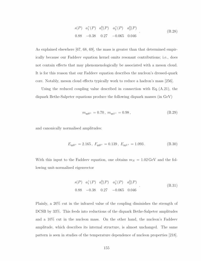
s(P ) a+1 (P ) a0
1(P ) a+2 (P ) a0
2(P )
0.88 −0.38 0.27 −0.065 0.046. (B.28)
As explained elsewhere [67, 68, 69], the mass is greater than that determined empir-
ically because our Faddeev equation kernel omits resonant contributions; i.e., does
not contain effects that may phenomenologically be associated with a meson cloud.
It is for this reason that our Faddeev equation describes the nucleon’s dressed-quark
core. Notably, meson cloud effects typically work to reduce a hadron’s mass [256].
Using the reduced coupling value described in connection with Eq. (A.21), the
diquark Bethe-Salpeter equations produce the following diquark masses (in GeV)
mqq0+ = 0.70 , mqq1+ = 0.98 , (B.29)
and canonically normalised amplitudes:
Eqq0+ = 2.165 , Fqq0+ = 0.139 , Eqq1+ = 1.093 . (B.30)
With this input to the Faddeev equation, one obtains mN = 1.02 GeV and the fol-
lowing unit-normalised eigenvector
s(P ) a+1 (P ) a0
1(P ) a+2 (P ) a0
2(P )
0.88 −0.38 0.27 −0.065 0.046. (B.31)
Plainly, a 20% cut in the infrared value of the coupling diminishes the strength of
DCSB by 33%. This feeds into reductions of the diquark Bethe-Salpeter amplitudes
and a 10% cut in the nucleon mass. On the other hand, the nucleon’s Faddeev
amplitude, which describes its internal structure, is almost unchanged. The same
pattern is seen in studies of the temperature dependence of nucleon properties [218].
155
APPENDIX C
INTERACTION CURRENTS
In this appendix we explain the interaction currents involved in the calculation of
nucleon static charges using the Fadeev equation. In order to translate the diagrams
drawn in this appendix into formulae, it is helpful to bear the following points in
mind.
(1) In front of a closed fermion trace; i.e., a vertex, one should, as usual, include a
factor of (−1).
(2a) States entering a diagram are described by the amplitudes
Γ0+
qq (P ) = γ5 (iEqq0+ +1
Mγ · P Fqq0+) , (C.1a)
Γ1+
qqµ(P ) = iEqq1+γTµ , (C.1b)
S(P ) = s I , (C.1c)
A jµ(P ) = aj
1γµγ5 + iaj2γ5Pµ . (C.1d)
(N.B. In this Appendix we have absorbed the “i” of Eqs. (B.5), (B.22) into the labels
Γ1+
qqµ(P ) and A jµ.)
(2b) States leaving a diagram are described by the amplitudes
Γ0+
qq (−P ) = γ5 (iEqq0+ − 1
Mγ · P Fqq0+) , (C.2a)
Γ1+
qqµ(−P ) = iEqq1+γTµ , (C.2b)
S(−P ) = s I =: S , (C.2c)
156
A jµ(−P ) = aj
1γ5γµ + iaj2γ5Pµ . (C.2d)
In these equations,
γTµ = γνPµν(P ) , Pµν(P ) = δµν +
PµPν
m2qq1+
. (C.3)
(3) In the traces arising from a closed fermion loop, we have: ejN for charge form
factors, where e0 = 13e, e+ = 4
3e, where e is the positron charge; and 2N for scalar
and tensor form factors. Note that N = 2 for diquark initial and final states.
C.1 Electromagnetic Current
In computing the charge form factor of any hadron, one must employ the dressed-
quark-photon vertex [257, 258]. That vertex may be obtained by solving an inho-
mogeneous Bethe-Salpeter equation whose unrenormalised form is determined by the
inhomogeneous term γµ. The complete solution for the contact-interaction’s vector
vertex in RL truncation can be found in Refs. [65, 216]; but that result is not neces-
sary herein because we only require the result at Q2 = 0, which is fixed by the Ward
identity. With the contact interaction, that means
V qµ (Q)
Q2=0= eqγµ , (C.4)
where eq is the quark’s electric charge.
The Q2 = 0 value of the elastic electromagnetic proton current determines the
canonical normalisation of the nucleon’s Faddeev amplitude [259]. Given the Faddeev
equation in Fig. 2.2, the complete result is obtained by summing the six one-loop
157
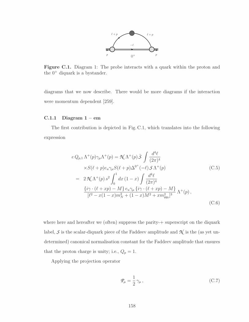
ℓ+ p
p p
−ℓ
0+
ℓ+ p
Figure C.1. Diagram 1: The probe interacts with a quark within the proton andthe 0+ diquark is a bystander.
diagrams that we now describe. There would be more diagrams if the interaction
were momentum dependent [259].
C.1.1 Diagram 1 – em
The first contribution is depicted in Fig. C.1, which translates into the following
expression
eQp,1 Λ+(p)γµΛ+(p) = N Λ+(p) S
∫
d4ℓ
(2π)4
×S(ℓ+ p)euγµS(ℓ+ p)∆0+
(−ℓ) S Λ+(p) (C.5)
= 2 N Λ+(p) s2
∫ 1
0
dx (1 − x)
∫
d4ℓ
(2π)4
iγ · (ℓ+ xp) −M euγµ iγ · (ℓ+ xp) −M[ℓ2 − x(1 − x)m2
N + (1 − x)M2 + xm2qq0
]3Λ+(p) ,
(C.6)
where here and hereafter we (often) suppress the parity-+ superscript on the diquark
label, S is the scalar-diquark piece of the Faddeev amplitude and N is the (as yet un-
determined) canonical normalisation constant for the Faddeev amplitude that ensures
that the proton charge is unity; i.e., Qp = 1.
Applying the projection operator
Pµ =1
2γµ , (C.7)
158
and performing the trace, one obtains
eQp,1 = eu N s2
∫ 1
0
dx (1 − x)
∫
d4ℓ
(2π)4
ℓ2 + 2(M + xmN)2
[ℓ2 − x(1 − x)m2N + (1 − x)M2 + xm2
qq0]3
(C.8)
→ eu N s2
∫ 1
0
dx (1 − x)
G iu2
(
x(x− 1)m2N
+(1 − x)M2 + xm2qq0
)
+ 2(M + xmN)2
×G iu1
(
x(x− 1)m2N + (1 − x)M2 + xm2
qq0
)
, (C.9)
where G iu1 (ω), G iu
2 (ω) are defined in Eqs. (A.14), (A.15), respectively, and eu = 23e.
This expression evaluates to
eQp,1 = D1 eu N
= 0.0182622 eu N = 0.0121748 eN . (C.10)
C.1.2 Diagram 2 – em
The second contribution is almost identical to that depicted in Fig. C.1: the only
change being that in this instance a 1+ diquark is the bystander. However, owing to
isospin symmetry, which we assume herein, and Eq. (B.25), this term yields
eQp,2 = (2 ed + eu)D02 N
= (2 ed + eu) 0.00195845 N = 0 , (C.11)
where D02 is the contribution obtained with a ud-diquark spectator.
C.1.3 Diagram 3 – em
The third contribution is depicted in Fig. C.2, which represents the following ex-
pression
159
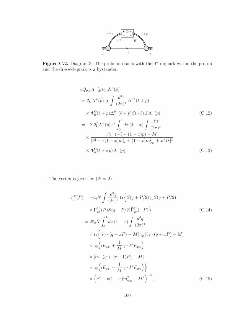
ℓ+ p
p p−ℓ
ℓ+ p
0+
0+
Figure C.2. Diagram 3: The probe interacts with the 0+ diquark within the protonand the dressed-quark is a bystander.
eQp,3 Λ+(p)γµΛ+(p)
= N Λ+(p) S
∫
d4ℓ
(2π)4∆0+
(ℓ+ p)
× V 0µ (ℓ+ p)∆0+
(ℓ+ p)S(−ℓ) S Λ+(p) (C.12)
= −2 N Λ+(p) s2
∫ 1
0
dx (1 − x)
∫
d4ℓ
(2π)4
× iγ · (−ℓ+ (1 − x)p) −M
[ℓ2 − x(1 − x)m2N + (1 − x)m2
qq0+ xM2]3
× V 0µ (ℓ+ xp) Λ+(p) . (C.13)
The vertex is given by (N = 2)
V 0µ (P ) = −e0N
∫
d4q
(2π)4tr
S(q + P/2)γµS(q + P/2)
× Γ0+
qq (P )S(q − P/2)Γ0+
qq (−P )
(C.14)
= 2e0N
∫ 1
0
dx (1 − x)
∫
d4q
(2π)4
× tr
[iγ · (q + xP ) −M ] γµ [iγ · (q + xP ) −M ]
× γ5
(
iEqq0+
1
Mγ · P Fqq0
)
× [iγ · (q + (x− 1)P ) −M ]
× γ5
(
iEqq0− 1
Mγ · P Fqq0
)
×(
q2 − x(1 − x)m2qq0
+M2)−3
, (C.15)
160
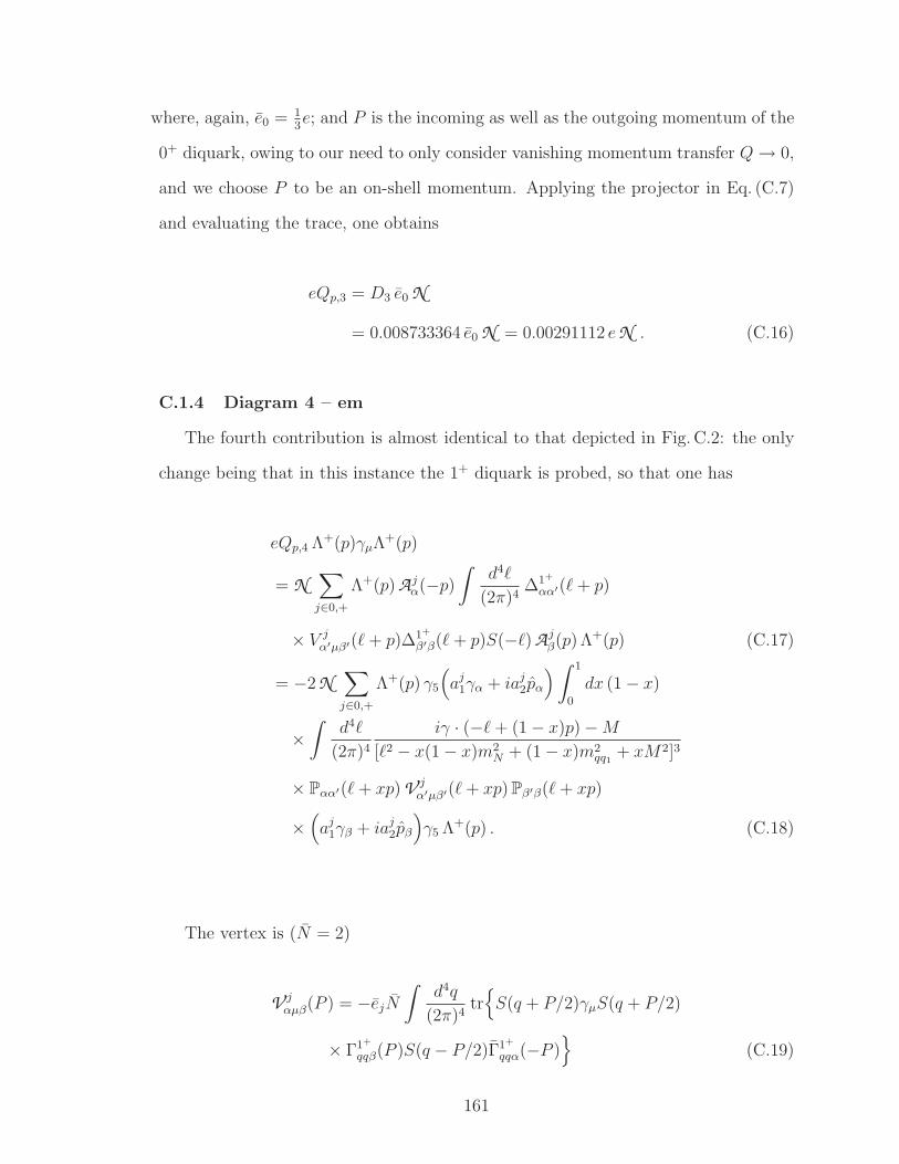
where, again, e0 = 13e; and P is the incoming as well as the outgoing momentum of the
0+ diquark, owing to our need to only consider vanishing momentum transfer Q→ 0,
and we choose P to be an on-shell momentum. Applying the projector in Eq. (C.7)
and evaluating the trace, one obtains
eQp,3 = D3 e0 N
= 0.008733364 e0 N = 0.00291112 eN . (C.16)
C.1.4 Diagram 4 – em
The fourth contribution is almost identical to that depicted in Fig. C.2: the only
change being that in this instance the 1+ diquark is probed, so that one has
eQp,4 Λ+(p)γµΛ+(p)
= N∑
j∈0,+
Λ+(p) A jα(−p)
∫
d4ℓ
(2π)4∆1+
αα′(ℓ+ p)
× V jα′µβ′(ℓ+ p)∆1+
β′β(ℓ+ p)S(−ℓ) A jβ(p) Λ+(p) (C.17)
= −2 N∑
j∈0,+
Λ+(p) γ5
(
aj1γα + iaj
2pα
)
∫ 1
0
dx (1 − x)
×∫
d4ℓ
(2π)4
iγ · (−ℓ+ (1 − x)p) −M
[ℓ2 − x(1 − x)m2N + (1 − x)m2
qq1+ xM2]3
× Pαα′(ℓ+ xp) V jα′µβ′(ℓ+ xp) Pβ′β(ℓ+ xp)
×(
aj1γβ + iaj
2pβ
)
γ5 Λ+(p) . (C.18)
The vertex is (N = 2)
V jαµβ(P ) = −ejN
∫
d4q
(2π)4tr
S(q + P/2)γµS(q + P/2)
× Γ1+
qqβ(P )S(q − P/2)Γ1+
qqα(−P )
(C.19)
161
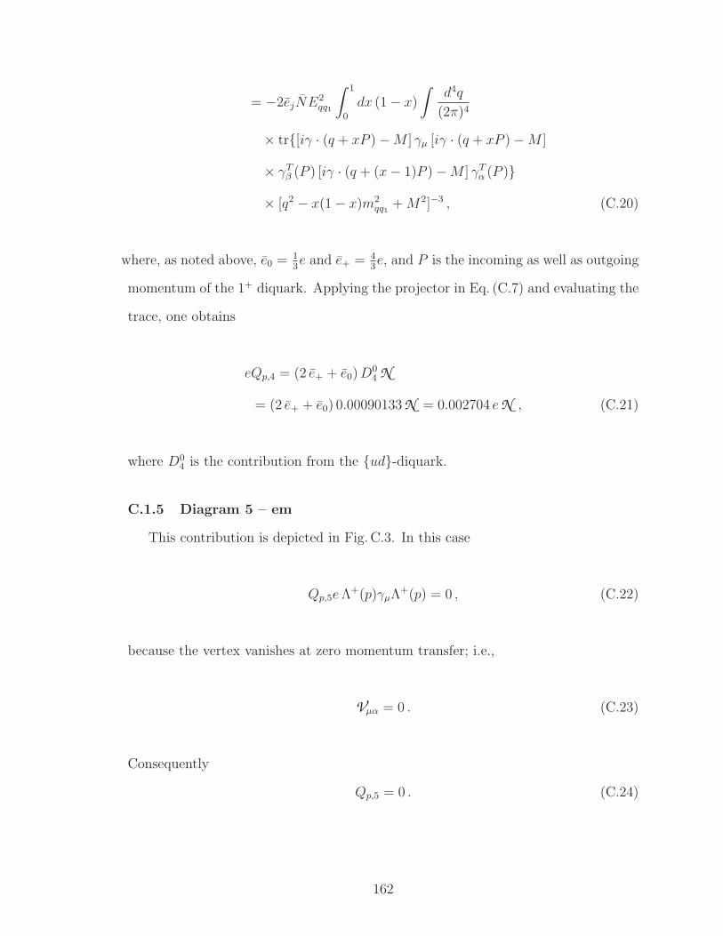
= −2ejNE2qq1
∫ 1
0
dx (1 − x)
∫
d4q
(2π)4
× tr[iγ · (q + xP ) −M ] γµ [iγ · (q + xP ) −M ]
× γTβ (P ) [iγ · (q + (x− 1)P ) −M ] γT
α (P )
× [q2 − x(1 − x)m2qq1
+M2]−3 , (C.20)
where, as noted above, e0 = 13e and e+ = 4
3e, and P is the incoming as well as outgoing
momentum of the 1+ diquark. Applying the projector in Eq. (C.7) and evaluating the
trace, one obtains
eQp,4 = (2 e+ + e0)D04 N
= (2 e+ + e0) 0.00090133 N = 0.002704 eN , (C.21)
where D04 is the contribution from the ud-diquark.
C.1.5 Diagram 5 – em
This contribution is depicted in Fig. C.3. In this case
Qp,5eΛ+(p)γµΛ+(p) = 0 , (C.22)
because the vertex vanishes at zero momentum transfer; i.e.,
Vµα = 0 . (C.23)
Consequently
Qp,5 = 0 . (C.24)
162
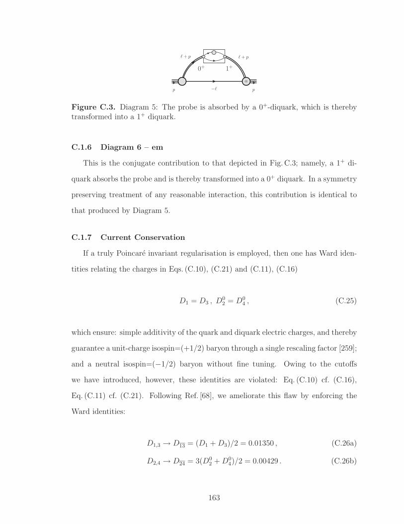
ℓ+ p
p p−ℓ
ℓ+ p
α
0+
1+
Figure C.3. Diagram 5: The probe is absorbed by a 0+-diquark, which is therebytransformed into a 1+ diquark.
C.1.6 Diagram 6 – em
This is the conjugate contribution to that depicted in Fig. C.3; namely, a 1+ di-
quark absorbs the probe and is thereby transformed into a 0+ diquark. In a symmetry
preserving treatment of any reasonable interaction, this contribution is identical to
that produced by Diagram 5.
C.1.7 Current Conservation
If a truly Poincare invariant regularisation is employed, then one has Ward iden-
tities relating the charges in Eqs. (C.10), (C.21) and (C.11), (C.16)
D1 = D3 , D02 = D0
4 , (C.25)
which ensure: simple additivity of the quark and diquark electric charges, and thereby
guarantee a unit-charge isospin=(+1/2) baryon through a single rescaling factor [259];
and a neutral isospin=(−1/2) baryon without fine tuning. Owing to the cutoffs
we have introduced, however, these identities are violated: Eq. (C.10) cf. (C.16),
Eq. (C.11) cf. (C.21). Following Ref. [68], we ameliorate this flaw by enforcing the
Ward identities:
D1,3 → D13 = (D1 +D3)/2 = 0.01350 , (C.26a)
D2,4 → D24 = 3(D02 +D0
4)/2 = 0.00429 . (C.26b)
163
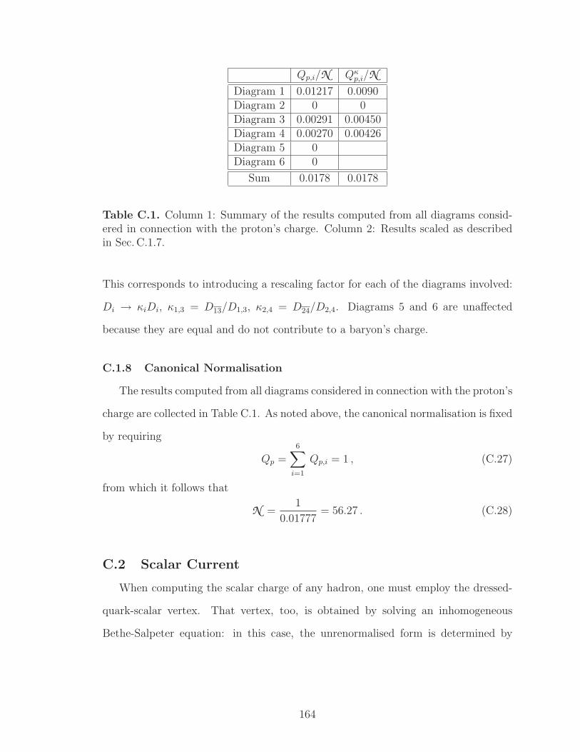
Qp,i/N Qκp,i/N
Diagram 1 0.01217 0.0090Diagram 2 0 0Diagram 3 0.00291 0.00450Diagram 4 0.00270 0.00426Diagram 5 0Diagram 6 0
Sum 0.0178 0.0178
Table C.1. Column 1: Summary of the results computed from all diagrams consid-ered in connection with the proton’s charge. Column 2: Results scaled as describedin Sec. C.1.7.
This corresponds to introducing a rescaling factor for each of the diagrams involved:
Di → κiDi, κ1,3 = D13/D1,3, κ2,4 = D24/D2,4. Diagrams 5 and 6 are unaffected
because they are equal and do not contribute to a baryon’s charge.
C.1.8 Canonical Normalisation
The results computed from all diagrams considered in connection with the proton’s
charge are collected in Table C.1. As noted above, the canonical normalisation is fixed
by requiring
Qp =6∑
i=1
Qp,i = 1 , (C.27)
from which it follows that
N =1
0.01777= 56.27 . (C.28)
C.2 Scalar Current
When computing the scalar charge of any hadron, one must employ the dressed-
quark-scalar vertex. That vertex, too, is obtained by solving an inhomogeneous
Bethe-Salpeter equation: in this case, the unrenormalised form is determined by
164
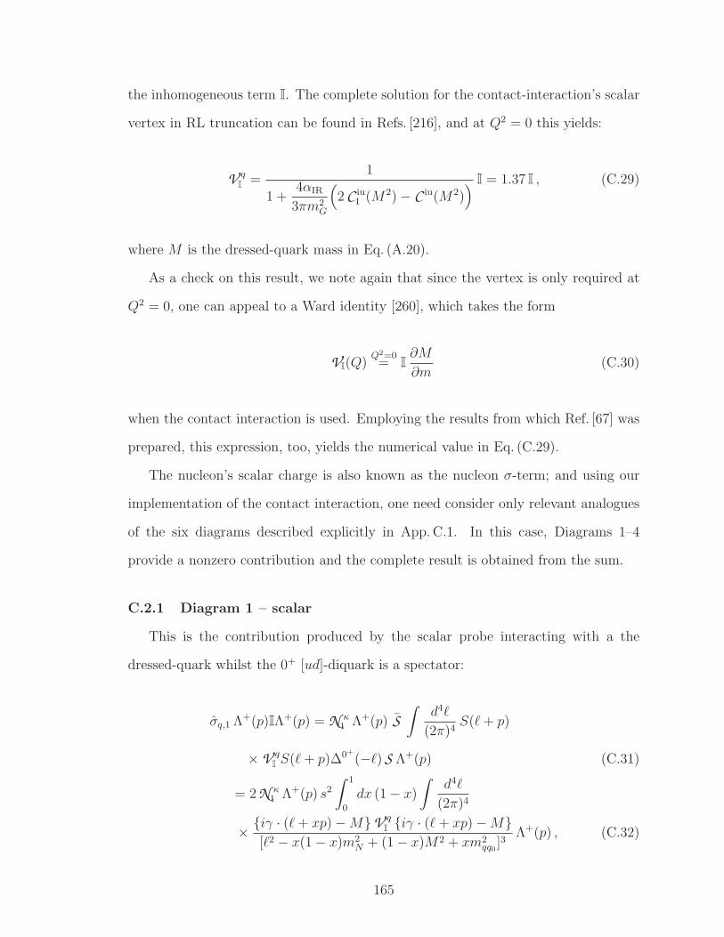
the inhomogeneous term I. The complete solution for the contact-interaction’s scalar
vertex in RL truncation can be found in Refs. [216], and at Q2 = 0 this yields:
V qI
=1
1 +4αIR
3πm2G
(
2 C iu1 (M2) − C iu(M2)
)I = 1.37 I , (C.29)
where M is the dressed-quark mass in Eq. (A.20).
As a check on this result, we note again that since the vertex is only required at
Q2 = 0, one can appeal to a Ward identity [260], which takes the form
VI(Q)Q2=0= I
∂M
∂m(C.30)
when the contact interaction is used. Employing the results from which Ref. [67] was
prepared, this expression, too, yields the numerical value in Eq. (C.29).
The nucleon’s scalar charge is also known as the nucleon σ-term; and using our
implementation of the contact interaction, one need consider only relevant analogues
of the six diagrams described explicitly in App. C.1. In this case, Diagrams 1–4
provide a nonzero contribution and the complete result is obtained from the sum.
C.2.1 Diagram 1 – scalar
This is the contribution produced by the scalar probe interacting with a the
dressed-quark whilst the 0+ [ud]-diquark is a spectator:
σq,1 Λ+(p)IΛ+(p) = N κ1 Λ+(p) S
∫
d4ℓ
(2π)4S(ℓ+ p)
× V qIS(ℓ+ p)∆0+
(−ℓ) S Λ+(p) (C.31)
= 2 N κ1 Λ+(p) s2
∫ 1
0
dx (1 − x)
∫
d4ℓ
(2π)4
× iγ · (ℓ+ xp) −MV qIiγ · (ℓ+ xp) −M
[ℓ2 − x(1 − x)m2N + (1 − x)M2 + xm2
qq0]3
Λ+(p) , (C.32)
165
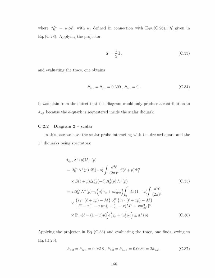
where N κ1 = κ1N , with κ1 defined in connection with Eqs. (C.26), N given in
Eq. (C.28). Applying the projector
P =1
2I , (C.33)
and evaluating the trace, one obtains
σu,1 = σq,1 = 0.309 , σd,1 = 0 . (C.34)
It was plain from the outset that this diagram would only produce a contribution to
σu,1 because the d-quark is sequestered inside the scalar diquark.
C.2.2 Diagram 2 – scalar
In this case we have the scalar probe interacting with the dressed-quark and the
1+ diquarks being spectators:
σqj,2Λ+(p)IΛ+(p)
= N κ2 Λ+(p) A j
α(−p)∫
d4ℓ
(2π)4S(ℓ+ p)V q
I
× S(ℓ+ p)∆1+
αβ(−ℓ) A jβ(p) Λ+(p) (C.35)
= 2 N κ2 Λ+(p) γ5
(
aj1γα + iaj
2pα
)
∫ 1
0
dx (1 − x)
∫
d4ℓ
(2π)4
× iγ · (ℓ+ xp) −MV qIiγ · (ℓ+ xp) −M
[ℓ2 − x(1 − x)m2N + (1 − x)M2 + xm2
qq1 ]3
× Pαβ(ℓ− (1 − x)p)(
aj1γβ + iaj
2pβ
)
γ5 Λ+(p). (C.36)
Applying the projector in Eq. (C.33) and evaluating the trace, one finds, owing to
Eq. (B.25),
σu,2 = σq0,2= 0.0318 , σd,2 = σq+,2
= 0.0636 = 2σu,2 . (C.37)
166
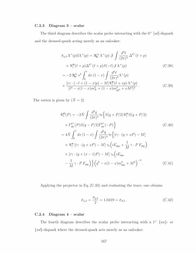
C.2.3 Diagram 3 – scalar
The third diagram describes the scalar probe interacting with the 0+ [ud]-diquark
and the dressed-quark acting merely as an onlooker:
σq,3 Λ+(p)IΛ+(p) = N κ3 Λ+(p) S
∫
d4ℓ
(2π)4∆0+
(ℓ+ p)
× V 0I(ℓ+ p)∆0+
(ℓ+ p)S(−ℓ) S Λ+(p) (C.38)
= −2 N κ3 s2
∫ 1
0
dx (1 − x)
∫
d4ℓ
(2π)4Λ+(p)
× [iγ · (−ℓ+ (1 − x)p) −M ]V 0I(ℓ+ xp) Λ+(p)
[ℓ2 − x(1 − x)m2N + (1 − x)m2
qq0 + xM2]3. (C.39)
The vertex is given by (N = 2)
V 0I(P ) = −2N
∫
d4q
(2π)4tr
S(q + P/2)V qIS(q + P/2)
× Γ0+
qq (P )S(q − P/2)Γ0+
qq (−P )
(C.40)
= 4N
∫ 1
0
dx (1 − x)
∫
d4q
(2π)4tr
[iγ · (q + xP ) −M ]
× V qI
[iγ · (q + xP ) −M ] γ5
(
iEqq0+
1
Mγ · P Fqq0
)
× [iγ · (q + (x− 1)P ) −M ] γ5
(
iEqq0
− 1
Mγ · P Fqq0
)(
q2 − x(1 − x)m2qq0
+M2)−3
. (C.41)
Applying the projector in Eq. (C.33) and evaluating the trace, one obtains
σu,3 =σq,3
2= 1.0419 = σd,3 . (C.42)
C.2.4 Diagram 4 – scalar
The fourth diagram describes the scalar probe interacting with a 1+ uu- or
ud-diquark where the dressed-quark acts merely as an onlooker:
167
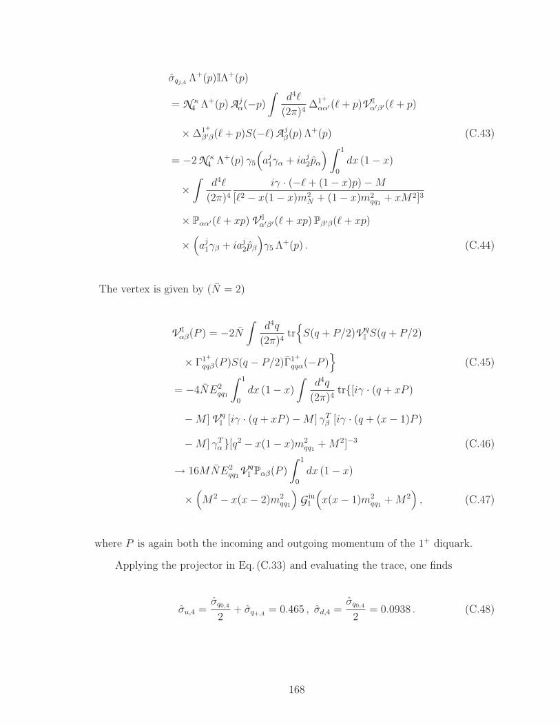
σqj,4Λ+(p)IΛ+(p)
= N κ4 Λ+(p) A j
α(−p)∫
d4ℓ
(2π)4∆1+
αα′(ℓ+ p)V I
α′β′(ℓ+ p)
× ∆1+
β′β(ℓ+ p)S(−ℓ) A jβ(p) Λ+(p) (C.43)
= −2 N κ4 Λ+(p) γ5
(
aj1γα + iaj
2pα
)
∫ 1
0
dx (1 − x)
×∫
d4ℓ
(2π)4
iγ · (−ℓ+ (1 − x)p) −M
[ℓ2 − x(1 − x)m2N + (1 − x)m2
qq1+ xM2]3
× Pαα′(ℓ+ xp) V I
α′β′(ℓ+ xp) Pβ′β(ℓ+ xp)
×(
aj1γβ + iaj
2pβ
)
γ5 Λ+(p) . (C.44)
The vertex is given by (N = 2)
V I
αβ(P ) = −2N
∫
d4q
(2π)4tr
S(q + P/2)V qIS(q + P/2)
× Γ1+
qqβ(P )S(q − P/2)Γ1+
qqα(−P )
(C.45)
= −4NE2qq1
∫ 1
0
dx (1 − x)
∫
d4q
(2π)4tr[iγ · (q + xP )
−M ] V qI
[iγ · (q + xP ) −M ] γTβ [iγ · (q + (x− 1)P )
−M ] γTα [q2 − x(1 − x)m2
qq1+M2]−3 (C.46)
→ 16MNE2qq1
V qIPαβ(P )
∫ 1
0
dx (1 − x)
×(
M2 − x(x− 2)m2qq1
)
G iu1
(
x(x− 1)m2qq1
+M2)
, (C.47)
where P is again both the incoming and outgoing momentum of the 1+ diquark.
Applying the projector in Eq. (C.33) and evaluating the trace, one finds
σu,4 =σq0,4
2+ σq+,4
= 0.465 , σd,4 =σq0,4
2= 0.0938 . (C.48)
168
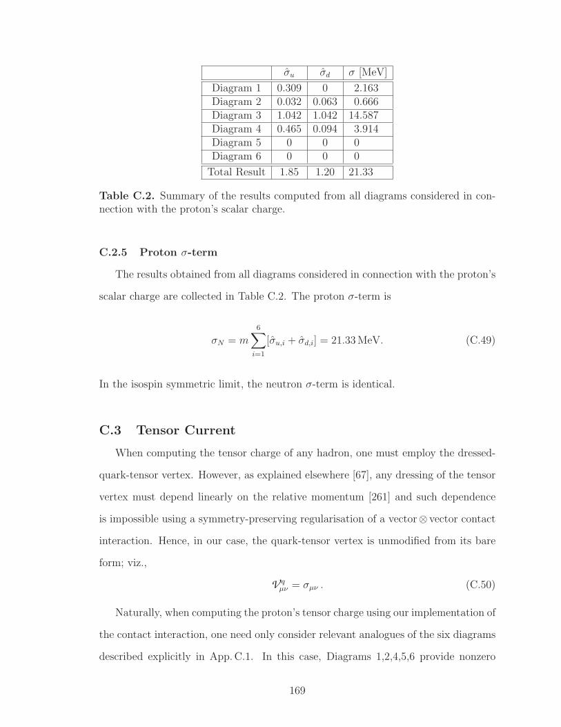
σu σd σ [MeV]
Diagram 1 0.309 0 2.163Diagram 2 0.032 0.063 0.666Diagram 3 1.042 1.042 14.587Diagram 4 0.465 0.094 3.914Diagram 5 0 0 0Diagram 6 0 0 0
Total Result 1.85 1.20 21.33
Table C.2. Summary of the results computed from all diagrams considered in con-nection with the proton’s scalar charge.
C.2.5 Proton σ-term
The results obtained from all diagrams considered in connection with the proton’s
scalar charge are collected in Table C.2. The proton σ-term is
σN = m6∑
i=1
[σu,i + σd,i] = 21.33 MeV. (C.49)
In the isospin symmetric limit, the neutron σ-term is identical.
C.3 Tensor Current
When computing the tensor charge of any hadron, one must employ the dressed-
quark-tensor vertex. However, as explained elsewhere [67], any dressing of the tensor
vertex must depend linearly on the relative momentum [261] and such dependence
is impossible using a symmetry-preserving regularisation of a vector⊗ vector contact
interaction. Hence, in our case, the quark-tensor vertex is unmodified from its bare
form; viz.,
V qµν = σµν . (C.50)
Naturally, when computing the proton’s tensor charge using our implementation of
the contact interaction, one need only consider relevant analogues of the six diagrams
described explicitly in App. C.1. In this case, Diagrams 1,2,4,5,6 provide nonzero
169
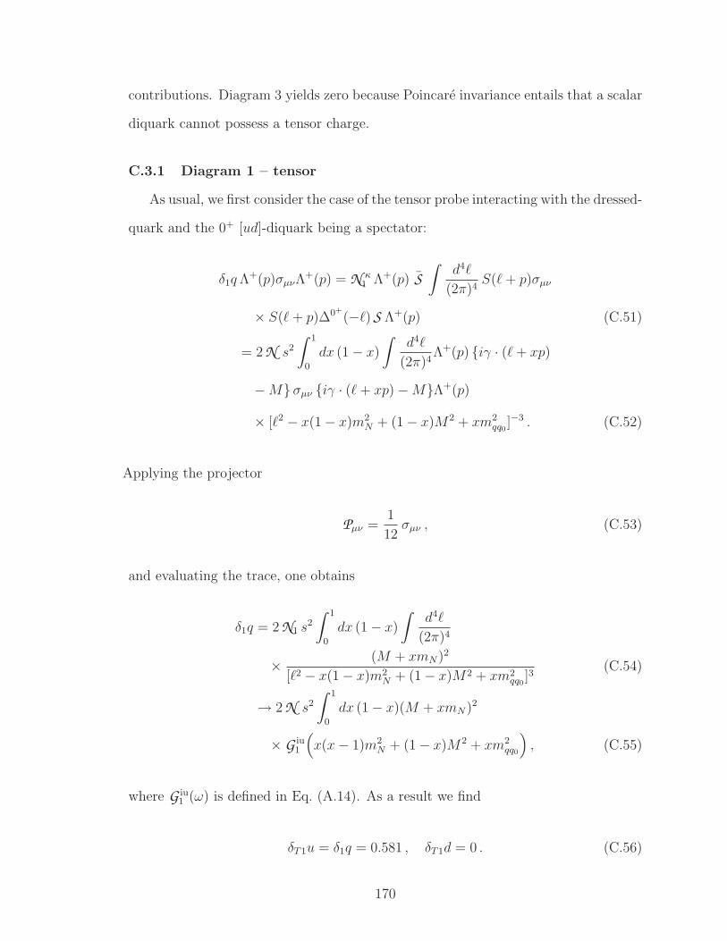
contributions. Diagram 3 yields zero because Poincare invariance entails that a scalar
diquark cannot possess a tensor charge.
C.3.1 Diagram 1 – tensor
As usual, we first consider the case of the tensor probe interacting with the dressed-
quark and the 0+ [ud]-diquark being a spectator:
δ1qΛ+(p)σµνΛ+(p) = N κ
1 Λ+(p) S
∫
d4ℓ
(2π)4S(ℓ+ p)σµν
× S(ℓ+ p)∆0+
(−ℓ) S Λ+(p) (C.51)
= 2 N s2
∫ 1
0
dx (1 − x)
∫
d4ℓ
(2π)4Λ+(p) iγ · (ℓ+ xp)
−Mσµν iγ · (ℓ+ xp) −MΛ+(p)
× [ℓ2 − x(1 − x)m2N + (1 − x)M2 + xm2
qq0]−3 . (C.52)
Applying the projector
Pµν =1
12σµν , (C.53)
and evaluating the trace, one obtains
δ1q = 2 N1 s2
∫ 1
0
dx (1 − x)
∫
d4ℓ
(2π)4
× (M + xmN)2
[ℓ2 − x(1 − x)m2N + (1 − x)M2 + xm2
qq0]3
(C.54)
→ 2 N s2
∫ 1
0
dx (1 − x)(M + xmN)2
× G iu1
(
x(x− 1)m2N + (1 − x)M2 + xm2
qq0
)
, (C.55)
where G iu1 (ω) is defined in Eq. (A.14). As a result we find
δT1u = δ1q = 0.581 , δT1d = 0 . (C.56)
170
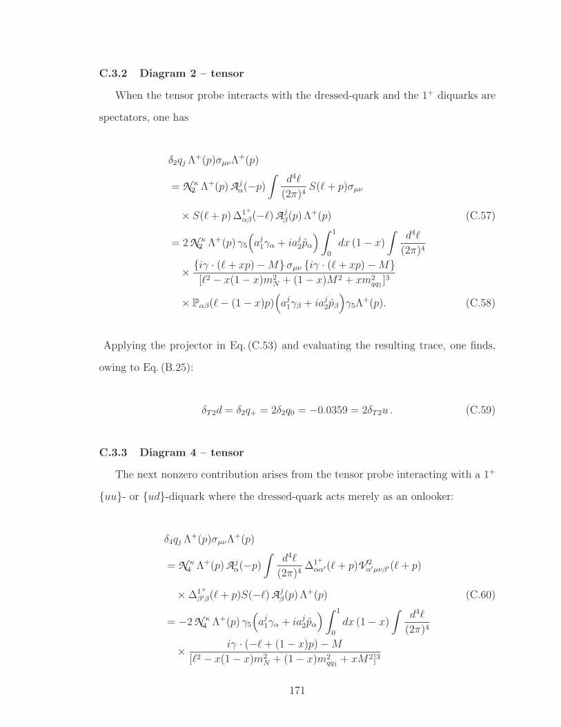
C.3.2 Diagram 2 – tensor
When the tensor probe interacts with the dressed-quark and the 1+ diquarks are
spectators, one has
δ2qj Λ+(p)σµνΛ+(p)
= N κ2 Λ+(p) A j
α(−p)∫
d4ℓ
(2π)4S(ℓ+ p)σµν
× S(ℓ+ p) ∆1+
αβ(−ℓ) A jβ(p) Λ+(p) (C.57)
= 2 N κ2 Λ+(p) γ5
(
aj1γα + iaj
2pα
)
∫ 1
0
dx (1 − x)
∫
d4ℓ
(2π)4
× iγ · (ℓ+ xp) −Mσµν iγ · (ℓ+ xp) −M[ℓ2 − x(1 − x)m2
N + (1 − x)M2 + xm2qq1
]3
× Pαβ(ℓ− (1 − x)p)(
aj1γβ + iaj
2pβ
)
γ5Λ+(p). (C.58)
Applying the projector in Eq. (C.53) and evaluating the resulting trace, one finds,
owing to Eq. (B.25):
δT2d = δ2q+ = 2δ2q0 = −0.0359 = 2δT2u . (C.59)
C.3.3 Diagram 4 – tensor
The next nonzero contribution arises from the tensor probe interacting with a 1+
uu- or ud-diquark where the dressed-quark acts merely as an onlooker:
δ4qj Λ+(p)σµνΛ+(p)
= N κ4 Λ+(p) A j
α(−p)∫
d4ℓ
(2π)4∆1+
αα′(ℓ+ p)V 2α′µνβ′(ℓ+ p)
× ∆1+
β′β(ℓ+ p)S(−ℓ) A jβ(p) Λ+(p) (C.60)
= −2 N κ4 Λ+(p) γ5
(
aj1γα + iaj
2pα
)
∫ 1
0
dx (1 − x)
∫
d4ℓ
(2π)4
× iγ · (−ℓ+ (1 − x)p) −M
[ℓ2 − x(1 − x)m2N + (1 − x)m2
qq1+ xM2]3
171
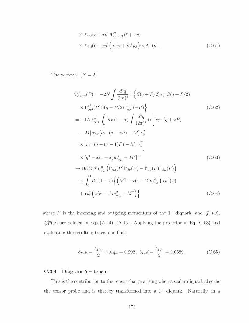
× Pαα′(ℓ+ xp) V 2α′µνβ′(ℓ+ xp)
× Pβ′β(ℓ+ xp)(
aj1γβ + iaj
2pβ
)
γ5 Λ+(p) . (C.61)
The vertex is (N = 2)
V 2αµνβ(P ) = −2N
∫
d4q
(2π)4tr
S(q + P/2)σµνS(q + P/2)
× Γ1+
qqβ(P )S(q − P/2)Γ1+
qqα(−P )
(C.62)
= −4NE2qq1
∫ 1
0
dx (1 − x)
∫
d4q
(2π)4tr
[
[iγ · (q + xP )
−M ]σµν [iγ · (q + xP ) −M ] γTβ
× [iγ · (q + (x− 1)P ) −M ] γTα
]
× [q2 − x(1 − x)m2qq1
+M2]−3 (C.63)
→ 16iMNE2qq1
(
Pαµ(P )Pβν(P ) − Pαν(P )Pβµ(P ))
×∫ 1
0
dx (1 − x)(
M2 − x(x− 2)m2qq1
)
G iu1 (ω)
+ G iu2
(
x(x− 1)m2qq1
+M2)
(C.64)
where P is the incoming and outgoing momentum of the 1+ diquark, and G iu1 (ω),
G iu2 (ω) are defined in Eqs. (A.14), (A.15). Applying the projector in Eq. (C.53) and
evaluating the resulting trace, one finds
δT4u =δ4q02
+ δ4q+ = 0.292 , δT4d =δ4q02
= 0.0589 . (C.65)
C.3.4 Diagram 5 – tensor
This is the contribution to the tensor charge arising when a scalar diquark absorbs
the tensor probe and is thereby transformed into a 1+ diquark. Naturally, in a
172
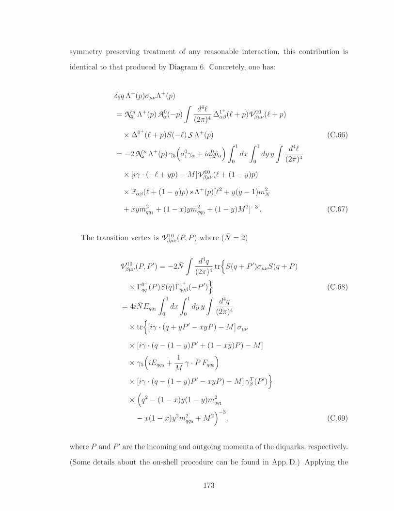
symmetry preserving treatment of any reasonable interaction, this contribution is
identical to that produced by Diagram 6. Concretely, one has:
δ5qΛ+(p)σµνΛ+(p)
= N κ5 Λ+(p) A0
α(−p)∫
d4ℓ
(2π)4∆1+
αβ(ℓ+ p)V 10βµν(ℓ+ p)
× ∆0+
(ℓ+ p)S(−ℓ) S Λ+(p) (C.66)
= −2 N κ5 Λ+(p) γ5
(
a01γα + ia0
2pα
)
∫ 1
0
dx
∫ 1
0
dy y
∫
d4ℓ
(2π)4
× [iγ · (−ℓ+ yp) −M ]V 10βµν(ℓ+ (1 − y)p)
× Pαβ(ℓ+ (1 − y)p) sΛ+(p)[ℓ2 + y(y − 1)m2N
+ xym2qq1
+ (1 − x)ym2qq0
+ (1 − y)M2]−3 . (C.67)
The transition vertex is V 10βµν(P, P ) where (N = 2)
V 10βµν(P, P
′) = −2N
∫
d4q
(2π)4tr
S(q + P ′)σµνS(q + P )
× Γ0+
qq (P )S(q)Γ1+
qqβ(−P ′)
(C.68)
= 4iNEqq1
∫ 1
0
dx
∫ 1
0
dy y
∫
d4q
(2π)4
× tr
[iγ · (q + yP ′ − xyP ) −M ]σµν
× [iγ · (q − (1 − y)P ′ + (1 − xy)P ) −M ]
× γ5
(
iEqq0+
1
Mγ · P Fqq0
)
× [iγ · (q − (1 − y)P ′ − xyP ) −M ] γTβ (P ′)
×(
q2 − (1 − x)y(1 − y)m2qq1
− x(1 − x)y2m2qq0
+M2)−3
, (C.69)
where P and P ′ are the incoming and outgoing momenta of the diquarks, respectively.
(Some details about the on-shell procedure can be found in App.D.) Applying the
173
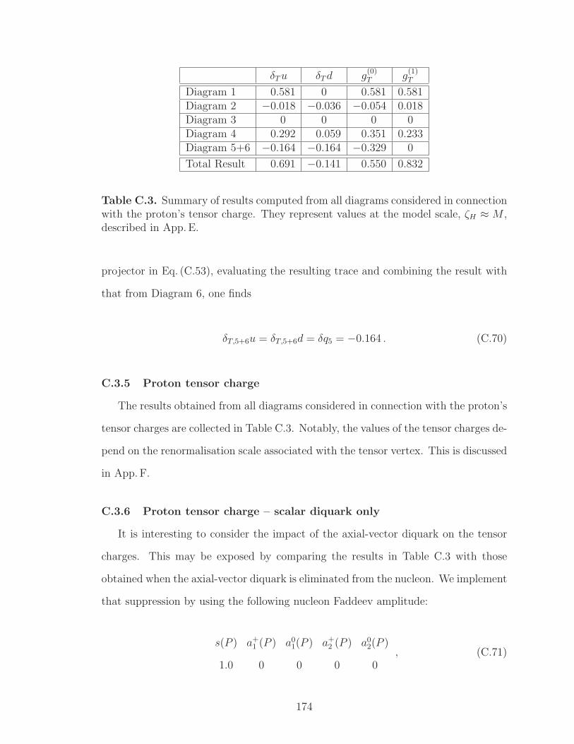
δTu δTd g(0)T g
(1)T
Diagram 1 0.581 0 0.581 0.581Diagram 2 −0.018 −0.036 −0.054 0.018Diagram 3 0 0 0 0Diagram 4 0.292 0.059 0.351 0.233Diagram 5+6 −0.164 −0.164 −0.329 0
Total Result 0.691 −0.141 0.550 0.832
Table C.3. Summary of results computed from all diagrams considered in connectionwith the proton’s tensor charge. They represent values at the model scale, ζH ≈ M ,described in App. E.
projector in Eq. (C.53), evaluating the resulting trace and combining the result with
that from Diagram 6, one finds
δT,5+6u = δT,5+6d = δq5 = −0.164 . (C.70)
C.3.5 Proton tensor charge
The results obtained from all diagrams considered in connection with the proton’s
tensor charges are collected in Table C.3. Notably, the values of the tensor charges de-
pend on the renormalisation scale associated with the tensor vertex. This is discussed
in App. F.
C.3.6 Proton tensor charge – scalar diquark only
It is interesting to consider the impact of the axial-vector diquark on the tensor
charges. This may be exposed by comparing the results in Table C.3 with those
obtained when the axial-vector diquark is eliminated from the nucleon. We implement
that suppression by using the following nucleon Faddeev amplitude:
s(P ) a+1 (P ) a0
1(P ) a+2 (P ) a0
2(P )
1.0 0 0 0 0, (C.71)
174
and then repeating the computations in Apps. C.1, C.3. Naturally, in this case only
Diagrams 1 and 3 can possibly yield nonzero contributions to any quantity.
Recomputing the canonical normalisation, we obtain
N6 1 =1
0.0174= 57.50 , (C.72)
which is 2% larger than the complete result in Eq. (C.28).
Regarding the tensor charges, Diagram 3 also vanishes in this instance so that the
net result is simply that produced by Diagram 1:
δT6 1u δT6 1d g(0)T6 1 g
(1)T6 1
0.765 0 0.765 0.765. (C.73)
Comparison with Table C.3 shows that with a symmetry-preserving treatment of a
vector⊗ vector contact interaction, the d-quark contribution to the proton’s tensor
charge is only nonzero in the presence of axial-vector diquark correlations and these
correlations reduce the u-quark contribution by 10%.
C.3.7 Proton tensor charge – Reduced DCSB
In order to expose the effect of DCSB on the tensor charges, we repeated all
relevant calculations above beginning with the value of αIR used to produce Eq. (A.21)
and thereby obtained the results listed in Table C.4.
175
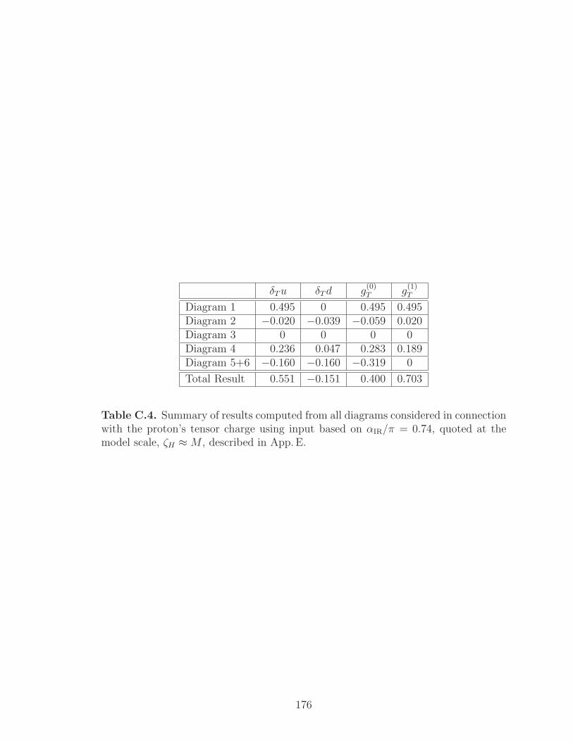
δTu δTd g(0)T g
(1)T
Diagram 1 0.495 0 0.495 0.495Diagram 2 −0.020 −0.039 −0.059 0.020Diagram 3 0 0 0 0Diagram 4 0.236 0.047 0.283 0.189Diagram 5+6 −0.160 −0.160 −0.319 0
Total Result 0.551 −0.151 0.400 0.703
Table C.4. Summary of results computed from all diagrams considered in connectionwith the proton’s tensor charge using input based on αIR/π = 0.74, quoted at themodel scale, ζH ≈M , described in App. E.
176
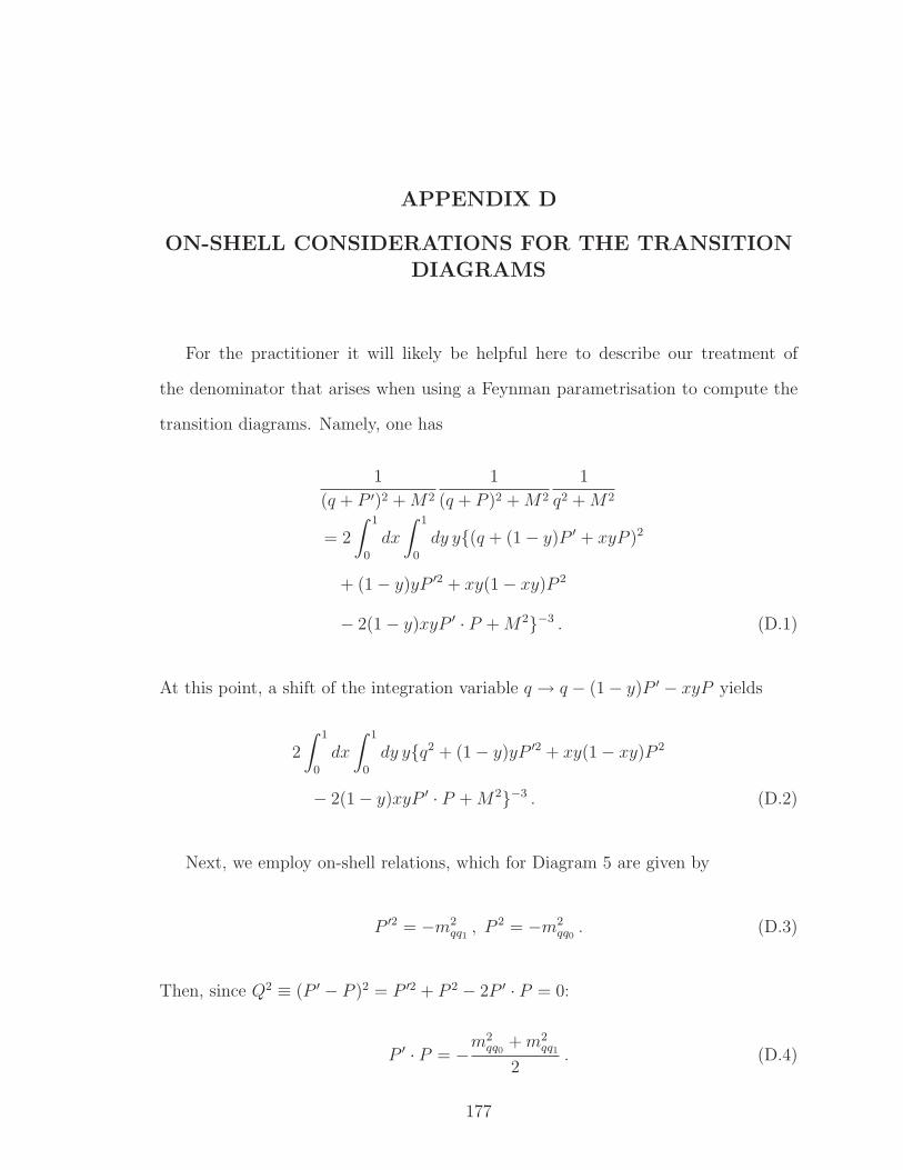
APPENDIX D
ON-SHELL CONSIDERATIONS FOR THE TRANSITION
DIAGRAMS
For the practitioner it will likely be helpful here to describe our treatment of
the denominator that arises when using a Feynman parametrisation to compute the
transition diagrams. Namely, one has
1
(q + P ′)2 +M2
1
(q + P )2 +M2
1
q2 +M2
= 2
∫ 1
0
dx
∫ 1
0
dy y(q + (1 − y)P ′ + xyP )2
+ (1 − y)yP ′2 + xy(1 − xy)P 2
− 2(1 − y)xyP ′ · P +M2−3 . (D.1)
At this point, a shift of the integration variable q → q − (1 − y)P ′ − xyP yields
2
∫ 1
0
dx
∫ 1
0
dy yq2 + (1 − y)yP ′2 + xy(1 − xy)P 2
− 2(1 − y)xyP ′ · P +M2−3 . (D.2)
Next, we employ on-shell relations, which for Diagram 5 are given by
P ′2 = −m2qq1, P 2 = −m2
qq0. (D.3)
Then, since Q2 ≡ (P ′ − P )2 = P ′2 + P 2 − 2P ′ · P = 0:
P ′ · P = −m2
qq0+m2
qq1
2. (D.4)
177
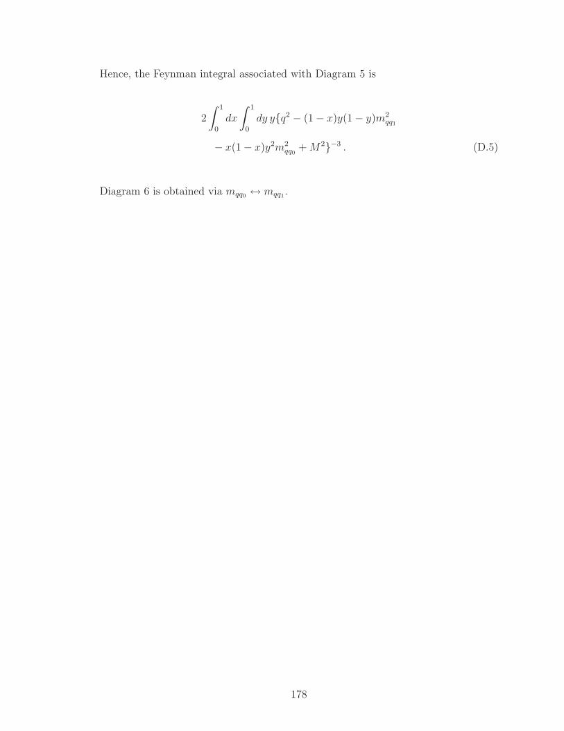
Hence, the Feynman integral associated with Diagram 5 is
2
∫ 1
0
dx
∫ 1
0
dy yq2 − (1 − x)y(1 − y)m2qq1
− x(1 − x)y2m2qq0
+M2−3 . (D.5)
Diagram 6 is obtained via mqq0↔ mqq1
.
178
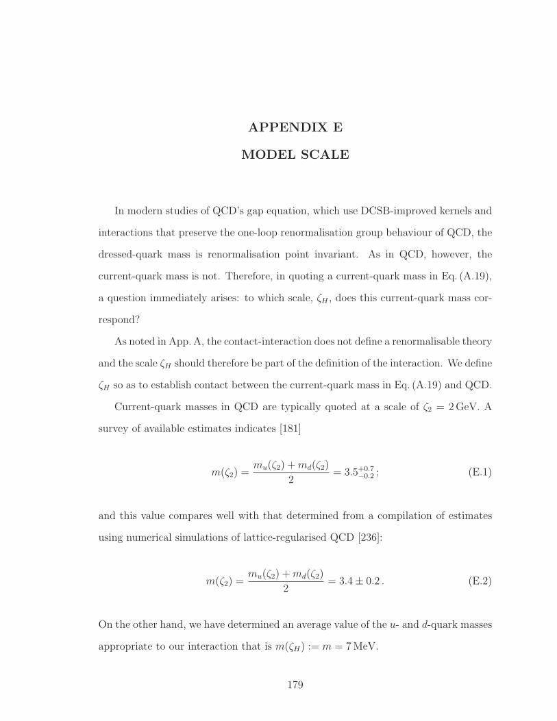
APPENDIX E
MODEL SCALE
In modern studies of QCD’s gap equation, which use DCSB-improved kernels and
interactions that preserve the one-loop renormalisation group behaviour of QCD, the
dressed-quark mass is renormalisation point invariant. As in QCD, however, the
current-quark mass is not. Therefore, in quoting a current-quark mass in Eq. (A.19),
a question immediately arises: to which scale, ζH , does this current-quark mass cor-
respond?
As noted in App. A, the contact-interaction does not define a renormalisable theory
and the scale ζH should therefore be part of the definition of the interaction. We define
ζH so as to establish contact between the current-quark mass in Eq. (A.19) and QCD.
Current-quark masses in QCD are typically quoted at a scale of ζ2 = 2 GeV. A
survey of available estimates indicates [181]
m(ζ2) =mu(ζ2) +md(ζ2)
2= 3.5+0.7
−0.2 ; (E.1)
and this value compares well with that determined from a compilation of estimates
using numerical simulations of lattice-regularised QCD [236]:
m(ζ2) =mu(ζ2) +md(ζ2)
2= 3.4 ± 0.2 . (E.2)
On the other hand, we have determined an average value of the u- and d-quark masses
appropriate to our interaction that is m(ζH) := m = 7 MeV.
179
The scale dependence of current-quark masses in QCD is expressed via
m(ζ ′)
m(ζ)=
[
αs(ζ′)
αs(ζ)
]γm
, (E.3)
where αs(ζ) is the running coupling and γm = 12/(33 − 2nf ), with nf the number
of active fermion flavours, is the mass anomalous dimension. Plainly, the running
current-quark mass increases as the scale is decreased.
Using the one-loop running coupling, with nf = 4 and ΛQCD = 0.234 GeV [83],
then
m(ζH) ≈ 2m(ζ2) for ζH = 0.39 ± 0.02 GeV ; (E.4)
and thus we have determined the model-scale. Given the arguments in Refs. [207,
262, 213], the outcome ζH ≈ M is both internally consistent and reasonable. (We
use the one-loop expression owing to the simplicity of our framework. Employing
next-to-leading-order (NLO) evolution leads simply to a 25% increase in ζH with no
material phenomenological differences.)
180
APPENDIX F
SCALE DEPENDENCE OF THE TENSOR CHARGE
Whilst the values of the tensor charges are gauge- and Poincare-invariant, they
depend on the renormalisation scale, ζ, employed to compute the dressed inhomoge-
neous tensor vertex
Γµν(k;Q; ζ) = S1(k;Q; ζ)σµν + . . . , (F.1)
at zero total momentum, Q = 0. (k is the relative momentum.) The renormalisation
constant ZT (ζ,Λ) is the factor required as a multiplier for the Bethe-Salpeter equation
inhomogeneity, σµν , in order to achieve S1(k2 = ζ2;Q = 0; ζ) = 1.
At one-loop order in QCD [263]:
Γµν(k;Q; ζ)ζ2≫Λ2
QCD
=
[
αS(ζ20 )
αS(ζ2)
]ηT
Γµν(k;Q; ζ0) , (F.2)
where ηT = (−1/3)γm. The pointwise behaviour of Γµν(k;Q = 0; ζ) is illustrated in
Ref. [238].
Equation (F.2) entails
δq(ζ)ζ2≫Λ2
QCD
=
[
αS(ζ20 )
αS(ζ2)
]ηT
δq(ζ0) , (F.3)
and hence that δq decreases as ζ increases. It follows, for example and in connection
with our analysis, that
δq(ζ2)
δq(ζH)= 0.794 ± 0.015 , (F.4)
with ζH drawn from Eq. (E.4).
181
APPENDIX G
EUCLIDEAN CONVENTIONS
The standard DSE treatment usually deals with Euclidean spacetime so it will be
worthwhile to explain the conventions here. In our Euclidean formulation:
p · q =4∑
i=1
piqi ; (G.1)
γµ, γν = 2 δµν ; ㆵ = γµ ; σµν =i
2[γµ, γν ] ; (G.2)
tr [γ5γµγνγργσ] = −4 ǫµνρσ , ǫ1234 = 1 . (G.3)
A positive energy spinor satisfies
u(P, s) (iγ · P +M) = 0 = (iγ · P +M) u(P, s) , (G.4)
where s = ±12
is the spin label. The spinor is normalised:
u(P, s) u(P, s) = 2M , (G.5)
and may be expressed explicitly:
u(P, s) =√M − iE
χs
~σ · ~PM − iE
χs
, (G.6)
182
with E = i√
~P 2 +M2,
χ+ =
1
0
, χ− =
0
1
. (G.7)
For the free-particle spinor, u(P, s) = u(P, s)†γ4.
The spinor can be used to construct a positive energy projection operator:
Λ+(P ) :=1
2M
∑
s=±u(P, s) u(P, s) =
1
2M(−iγ · P +M) . (G.8)
A charge-conjugated Bethe-Salpeter amplitude is obtained via
Γ(k;P ) = C† Γ(−k;P )TC , (G.9)
where “T” denotes a transposing of all matrix indices and C = γ2γ4 is the charge
conjugation matrix, C† = −C. We note that
C†γTµ C = −γµ , [C, γ5] = 0 . (G.10)
183
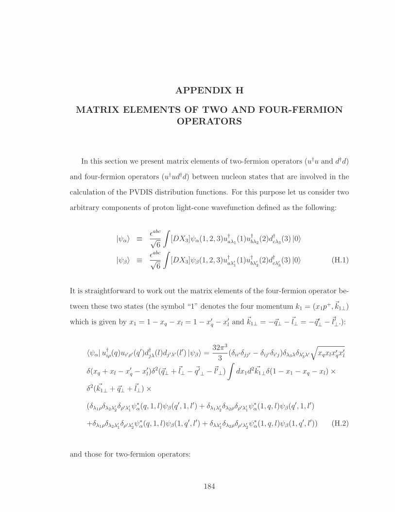
APPENDIX H
MATRIX ELEMENTS OF TWO AND FOUR-FERMION
OPERATORS
In this section we present matrix elements of two-fermion operators (u†u and d†d)
and four-fermion operators (u†ud†d) between nucleon states that are involved in the
calculation of the PVDIS distribution functions. For this purpose let us consider two
arbitrary components of proton light-cone wavefunction defined as the following:
|ψα〉 ≡ ǫabc
√6
∫
[DX3]ψα(1, 2, 3)u†aλ1(1)u†bλ2
(2)d†cλ3(3) |0〉
|ψβ〉 ≡ ǫabc
√6
∫
[DX3]ψβ(1, 2, 3)u†aλ′
1(1)u†bλ′
2(2)d†cλ′
3(3) |0〉 (H.1)
It is straightforward to work out the matrix elements of the four-fermion operator be-
tween these two states (the symbol “1” denotes the four momentum k1 = (x1p+, ~k1⊥)
which is given by x1 = 1 − xq − xl = 1 − x′q − x′l and ~k1⊥ = −~q⊥ −~l⊥ = −~q′⊥ −~l′⊥.):
〈ψα|u†iρ(q)ui′ρ′(q′)d†jλ(l)dj′λ′(l′) |ψβ〉 =
32π3
3(δii′δjj′ − δij′δi′j)δλ3λδλ′
3λ′
√
xqxlx′qx′l
δ(xq + xl − x′q − x′l)δ2(~q⊥ +~l⊥ − ~q′⊥ − ~l′⊥)
∫
dx1d2 ~k1⊥δ(1 − x1 − xq − xl) ×
δ2(~k1⊥ + ~q⊥ +~l⊥) ×
(δλ1ρδλ2λ′
2δρ′λ′
1ψ∗
α(q, 1, l)ψβ(q′, 1, l′) + δλ1λ′
2δλ2ρδρ′λ′
1ψ∗
α(1, q, l)ψβ(q′, 1, l′)
+δλ1ρδλ2λ′
1δρ′λ′
2ψ∗
α(q, 1, l)ψβ(1, q′, l′) + δλλ′
1δλ2ρδρ′λ′
2ψ∗
α(1, q, l)ψβ(1, q′, l′)) (H.2)
and those for two-fermion operators:
184
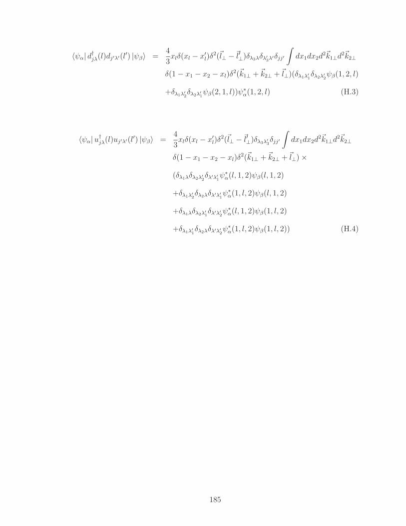
〈ψα| d†jλ(l)dj′λ′(l′) |ψβ〉 =4
3xlδ(xl − x′l)δ
2(~l⊥ −~l′⊥)δλ3λδλ′
3λ′δjj′
∫
dx1dx2d2~k1⊥d
2~k2⊥
δ(1 − x1 − x2 − xl)δ2(~k1⊥ + ~k2⊥ +~l⊥)(δλ1λ′
1δλ2λ′
2ψβ(1, 2, l)
+δλ1λ′
2δλ2λ′
1ψβ(2, 1, l))ψ∗
α(1, 2, l) (H.3)
〈ψα|u†jλ(l)uj′λ′(l′) |ψβ〉 =4
3xlδ(xl − x′l)δ
2(~l⊥ −~l′⊥)δλ3λ′
3δjj′
∫
dx1dx2d2~k1⊥d
2~k2⊥
δ(1 − x1 − x2 − xl)δ2(~k1⊥ + ~k2⊥ +~l⊥) ×
(δλ1λδλ2λ′
2δλ′λ′
1ψ∗
α(l, 1, 2)ψβ(l, 1, 2)
+δλ1λ′
2δλ2λδλ′λ′
1ψ∗
α(1, l, 2)ψβ(l, 1, 2)
+δλ1λδλ2λ′
1δλ′λ′
2ψ∗
α(l, 1, 2)ψβ(1, l, 2)
+δλ1λ′
1δλ2λδλ′λ′
2ψ∗
α(1, l, 2)ψβ(1, l, 2)) (H.4)
185
APPENDIX I
COMPLETE FORMULAE FOR VARIOUS QUARK
DISTRIBUTION FUNCTIONS IN TERMS OF PROTON
WAVEFUNCTION AMPLITUDES
In this section we present explicit expressions needed to compute the quark PDFs
and the twist-four distribution function.
The distribution functions Q±p (xB) in Eqs. (6.30) and (6.31) are expressed in terms
of ψ±lz(q, l, q′, l′), which have the following expressions:
186
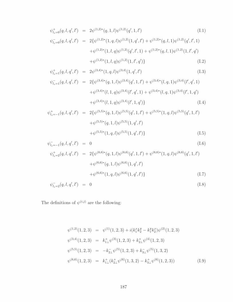
ψ+lz=0(q, l, q
′, l′) = 2ψ(1,2)∗(q, 1, l)ψ(1,2)(q′, 1, l′) (I.1)
ψ−lz=0(q, l, q
′, l′) = 2ψ(1,2)∗(1, q, l)ψ(1,2)(1, q′, l′) + ψ(1,2)∗(q, l, 1)ψ(1,2)(q′, l′, 1)
+ψ(1,2)∗(1, l, q)ψ(1,2)(q′, l′, 1) + ψ(1,2)∗(q, l, 1)ψ(1,2)(1, l′, q′)
+ψ(1,2)∗(1, l, q)ψ(1,2)(1, l′, q′) (I.2)
ψ+lz=1(q, l, q
′, l′) = 2ψ(3,4)∗(1, q, l)ψ(3,4)(1, q′, l′) (I.3)
ψ−lz=1(q, l, q
′, l′) = 2ψ(3,4)∗(q, 1, l)ψ(3,4)(q′, 1, l′) + ψ(3,4)∗(l, q, 1)ψ(3,4)(l′, q′, 1)
+ψ(3,4)∗(l, 1, q)ψ(3,4)(l′, q′, 1) + ψ(3,4)∗(l, q, 1)ψ(3,4)(l′, 1, q′)
+ψ(3,4)∗(l, 1, q)ψ(3,4)(l′, 1, q′) (I.4)
ψ+lz=−1(q, l, q
′, l′) = 2ψ(5,5)∗(q, 1, l)ψ(5,5)(q′, 1, l′) + ψ(5,5)∗(1, q, l)ψ(5,5)(q′, 1, l′)
+ψ(5,5)∗(q, 1, l)ψ(5,5)(1, q′, l′)
+ψ(5,5)∗(1, q, l)ψ(5,5)(1, q′, l′) (I.5)
ψ−lz=−1(q, l, q
′, l′) = 0 (I.6)
ψ+lz=2(q, l, q
′, l′) = 2ψ(6,6)∗(q, 1, l)ψ(6,6)(q′, 1, l′) + ψ(6,6)∗(1, q, l)ψ(6,6)(q′, 1, l′)
+ψ(6,6)∗(q, 1, l)ψ(6,6)(1, q′, l′)
+ψ(6,6)∗(1, q, l)ψ(6,6)(1, q′, l′) (I.7)
ψ−lz=2(q, l, q
′, l′) = 0 (I.8)
The definitions of ψ(i,j) are the following:
ψ(1,2)(1, 2, 3) = ψ(1)(1, 2, 3) + i(kx1k
y2 − ky
1kx2 )ψ(2)(1, 2, 3)
ψ(3,4)(1, 2, 3) = k+1⊥ψ
(3)(1, 2, 3) + k+2⊥ψ
(4)(1, 2, 3)
ψ(5,5)(1, 2, 3) = −k−2⊥ψ(5)(1, 2, 3) + k−3⊥ψ(5)(1, 3, 2)
ψ(6,6)(1, 2, 3) = k+1⊥(k+
2⊥ψ(6)(1, 3, 2) − k+
3⊥ψ(6)(1, 2, 3)) (I.9)
187
On the other hand, the quark distribution functions in (6.28) are given in terms
of Alz(q, 1, 2), which look like the following:
Alz=0(q, 1, 2) = ψ(1,2)∗(q, 1, 2)ψ(1,2)(q, 1, 2) + 2ψ(1,2)∗(1, q, 2)ψ(1,2)(1, q, 2)
+ψ(1,2)∗(q, 2, 1)ψ(1,2)(q, 2, 1) + ψ(1,2)∗(1, 2, q)ψ(1,2)(q, 2, 1)
+ψ(1,2)∗(q, 2, 1)ψ(1,2)(1, 2, q) + 2ψ(1,2)∗(1, 2, q)ψ(1,2)(1, 2, q)
+ψ(1,2)∗(1, q, 2)ψ(1,2)(2, q, 1) (I.10)
Alz=1(q, 1, 2) = 2ψ(3,4)∗(q, 1, 2)ψ(3,4)(q, 1, 2) + ψ(3,4)∗(1, q, 2)ψ(3,4)(1, q, 2)
+ψ(3,4)∗(2, q, 1)ψ(3,4)(2, q, 1) + ψ(3,4)∗(2, 1, q)ψ(3,4)(2, q, 1)
+ψ(3,4)∗(2, q, 1)ψ(3,4)(2, 1, q) + ψ(3,4)∗(2, 1, q)ψ(3,4)(2, 1, q)
+ψ(3,4)∗(1, 2, q)ψ(3,4)(1, 2, q)
+ψ(3,4)∗(q, 1, 2)ψ(3,4)(q, 2, 1) (I.11)
Alz=−1(q, 1, 2) = ψ(5,5)∗(q, 1, 2)ψ(5,5)(q, 1, 2) + ψ(5,5)∗(1, q, 2)ψ(5,5)(q, 1, 2)
+ψ(5,5)∗(q, 1, 2)ψ(5,5)(1, q, 2) + ψ(5,5)∗(1, q, 2)ψ(5,5)(1, q, 2)
+ψ(5,5)∗(1, 2, q)ψ(5,5)(1, 2, q)
+ψ(5,5)∗(1, 2, q)ψ(5,5)(2, 1, q) (I.12)
Alz=2(q, 1, 2) = ψ(6,6)∗(q, 1, 2)ψ(6,6)(q, 1, 2) + ψ(6,6)∗(1, q, 2)ψ(6,6)(q, 1, 2)
+ψ(6,6)∗(q, 1, 2)ψ(6,6)(1, q, 2) + ψ(6,6)∗(1, q, 2)ψ(6,6)(1, q, 2)
+ψ(6,6)∗(1, 2, q)ψ(6,6)(1, 2, q)
+ψ(6,6)∗(1, 2, q)ψ(6,6)(2, 1, q) (I.13)
188
with q = (xBp+, ~q⊥), x2 = 1 − xB − x1 and ~k2⊥ = −~q⊥ − ~k1⊥.
189
APPENDIX J
VANISHING ONE-LOOP DIAGRAMS IN THE
CALCULATIONS OF SM NUCLEON EDM
Here I will show that all 1-loop diagrams, other than those in Fig. 5.1, do not
give rise to the CKM-induced SM nucleon EDM, at least at leading order in the
HB-expansion.
All other possible 1-loop diagrams beside those I have calculated are summarized
in Fig. J.1. Since the weak Lagrangian used in my work does not involve covariant
derivatives of baryon fields, any baryon-photon coupling term has to arise from the
ordinary P and T-conserving Lagrangian.
For Fig. 4(a), the photon vertex must arise from Dirac coupling since an MDM
coupling is suppressed by (1/mN)2 as pointed out in [185]. Since the Dirac coupling
is independent of the photon momentum q, one can define loop momenta in a way
such that the dependence of q only appears in the baryon propagator. However, using
the on-shell condition v · q = 0, the baryon propagator is actually q-independent and
therefore so is the whole diagram. As a result, Fig. 4(a) cannot generate an EDM
that is linear in q.
For Fig. 4(b), at leading order in the HB-expansion the BB′φγ vertex is propor-
tional to Sµ, so it cannot generate an EDM because the latter is proportional to vµ
which is perpendicular to Sµ.
For Fig. 4(c), first I note that the BB′φφ′ vertex cannot come from the D or
F -term of the ordinary chiral Lagrangian because that would violate parity. There-
fore it can only come from L (s)w . In this case, it can only be parity-conserving and
190
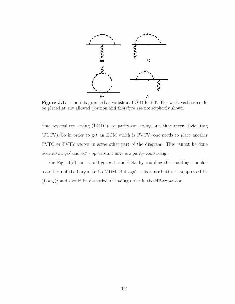
Figure J.1. 1-loop diagrams that vanish at LO HBchPT. The weak vertices couldbe placed at any allowed position and therefore are not explicitly shown.
time reversal-conserving (PCTC), or parity-conserving and time reversal-violating
(PCTV). So in order to get an EDM which is PVTV, one needs to place another
PVTC or PVTV vertex in some other part of the diagram. This cannot be done
because all φφ′ and φφ′γ operators I have are parity-conserving.
For Fig. 4(d), one could generate an EDM by coupling the resulting complex
mass term of the baryon to its MDM. But again this contribution is suppressed by
(1/mN)2 and should be discarded at leading order in the HB-expansion.
191
BIBLIOGRAPHY
[1] G. Arnison et al. [UA1 Collaboration], Phys. Lett. B 122 (1983) 103.
[2] M. Banner et al. [UA2 Collaboration], Phys. Lett. B 122 (1983) 476.
[3] J. E. Augustin et al. [SLAC-SP-017 Collaboration], Phys. Rev. Lett. 33 (1974)1406 [Adv. Exp. Phys. 5 (1976) 141].
[4] J. J. Aubert et al. [E598 Collaboration], Phys. Rev. Lett. 33 (1974) 1404.
[5] S. W. Herb, D. C. Hom, L. M. Lederman, J. C. Sens, H. D. Snyder, J. K. Yoh,J. A. Appel and B. C. Brown et al., Phys. Rev. Lett. 39 (1977) 252.
[6] F. Abe et al. [CDF Collaboration], Phys. Rev. Lett. 74 (1995) 2626 [hep-ex/9503002].
[7] S. Abachi et al. [D0 Collaboration], Phys. Rev. Lett. 74 (1995) 2422 [hep-ex/9411001].
[8] G. Aad et al. [ATLAS Collaboration], Phys. Lett. B 716 (2012) 1[arXiv:1207.7214 [hep-ex]].
[9] S. Chatrchyan et al. [CMS Collaboration], Phys. Lett. B 716 (2012) 30[arXiv:1207.7235 [hep-ex]].
[10] R. Davis, Jr., D. S. Harmer and K. C. Hoffman, Phys. Rev. Lett. 20 (1968)1205.
[11] Q. R. Ahmad et al. [SNO Collaboration], Phys. Rev. Lett. 87 (2001) 071301[nucl-ex/0106015].
[12] V. C. Rubin and W. K. Ford, Jr., Astrophys. J. 159 (1970) 379.
[13] V. C. Rubin, N. Thonnard and W. K. Ford, Jr., Astrophys. J. 238 (1980) 471.
[14] D. Clowe, M. Bradac, A. H. Gonzalez, M. Markevitch, S. W. Randall, C. Jonesand D. Zaritsky, Astrophys. J. 648 (2006) L109 [astro-ph/0608407].
[15] E. Komatsu et al. [WMAP Collaboration], Astrophys. J. Suppl. 192 (2011) 18[arXiv:1001.4538 [astro-ph.CO]].
[16] P. A. R. Ade et al. [Planck Collaboration], Astron. Astrophys. 571 (2014) A16[arXiv:1303.5076 [astro-ph.CO]].
192
[17] D. Hanneke, S. F. Hoogerheide and G. Gabrielse, Phys. Rev. A 83 (2011) 052122[arXiv:1009.4831 [physics.atom-ph]].
[18] T. Aoyama, M. Hayakawa, T. Kinoshita and M. Nio, Phys. Rev. Lett. 109
(2012) 111807 [arXiv:1205.5368 [hep-ph]].
[19] C. Y. Prescott, W. B. Atwood, R. L. Cottrell, H. C. DeStaebler, E. L. Garwin,A. Gonidec, R. H. Miller and L. S. Rochester et al., Phys. Lett. B 77 (1978)347.
[20] S. Schael et al. [ALEPH and DELPHI and L3 and OPAL and SLD and LEPElectroweak Working Group and SLD Electroweak Group and SLD HeavyFlavour Group Collaborations], Phys. Rept. 427 (2006) 257 [hep-ex/0509008].
[21] F. Jegerlehner and A. Nyffeler, Phys. Rept. 477 (2009) 1 [arXiv:0902.3360 [hep-ph]].
[22] C. S. Wu, E. Ambler, R. W. Hayward, D. D. Hoppes and R. P. Hudson, Phys.Rev. 105 (1957) 1413.
[23] J. H. Christenson, J. W. Cronin, V. L. Fitch and R. Turlay, Phys. Rev. Lett.13 (1964) 138.
[24] M. Kobayashi and T. Maskawa, Prog. Theor. Phys. 49 (1973) 652.
[25] Y. Fukuda et al. [Super-Kamiokande Collaboration], Phys. Rev. Lett. 81 (1998)1562 [hep-ex/9807003].
[26] F. P. An et al. [Daya Bay Collaboration], Phys. Rev. Lett. 108 (2012) 171803[arXiv:1203.1669 [hep-ex]].
[27] J. K. Ahn et al. [RENO Collaboration], Phys. Rev. Lett. 108 (2012) 191802[arXiv:1204.0626 [hep-ex]].
[28] S. Weinberg, “The quantum theory of fields. Vol. 2: Modern applications, Cam-bridge, UK: Univ. Pr. (1996) 489 p
[29] B. Grzadkowski, M. Iskrzynski, M. Misiak and J. Rosiek, JHEP 1010 (2010)085 [arXiv:1008.4884 [hep-ph]].
[30] D. J. Gross and F. Wilczek, Phys. Rev. Lett. 30 (1973) 1343.
[31] H. D. Politzer, Phys. Rev. Lett. 30 (1973) 1346.
[32] K. G. Wilson, Phys. Rev. D 10 (1974) 2445.
[33] J. H. Smith, E. M. Purcell and N. F. Ramsey, Phys. Rev. 108 (1957) 120.
[34] G. ’t Hooft, Phys. Rev. Lett. 37 (1976) 8.
[35] R. D. Peccei and H. R. Quinn, Phys. Rev. Lett. 38 (1977) 1440.
193
[36] A. E. Nelson, Phys. Lett. B 136 (1984) 387.
[37] S. M. Barr, Phys. Rev. Lett. 53 (1984) 329.
[38] A. D. Sakharov, Pisma Zh. Eksp. Teor. Fiz. 5 (1967) 32 [JETP Lett. 5 (1967)24] [Sov. Phys. Usp. 34 (1991) 392] [Usp. Fiz. Nauk 161 (1991) 61].
[39] M. B. Gavela, P. Hernandez, J. Orloff and O. Pene, Mod. Phys. Lett. A 9 (1994)795 [hep-ph/9312215, hep-ph/9312215].
[40] P. Huet and E. Sather, Phys. Rev. D 51 (1995) 379 [hep-ph/9404302].
[41] see e.g. M. Gonzlez-Alonso and J. Martin Camalich, Phys. Rev. Lett. 112 (2014)4, 042501 [arXiv:1309.4434 [hep-ph]] and the references therein.
[42] P. Langacker, “Precision tests of the standard electroweak model,” Singapore,Singapore: World Scientific (1995) 1008 p. (Advanced series on directions inhigh energy physics: 14)
[43] J. D. Jackson, S. B. Treiman and H. W. Wyld, Phys. Rev. 106 (1957) 517.
[44] H. P. Mumm, T. E. Chupp, R. L. Cooper, K. P. Coulter, S. J. Freedman,B. K. Fujikawa, A. Garcia and G. L. Jones et al., Phys. Rev. Lett. 107 (2011)102301 [arXiv:1104.2778 [nucl-ex]].
[45] M. Anselmino, M. Boglione, U. D’Alesio, S. Melis, F. Murgia and A. Prokudin,Phys. Rev. D 87 (2013) 094019 [arXiv:1303.3822 [hep-ph]].
[46] P. Bosted et al., Jefferson-Lab proposal PR-09-012, Precision Measurementof Parity-violation in Deep Inelastic Scattering Over a Broad KinematicRange, http://hallaweb.jlab.org/collab/PAC/PAC34/PR-09-012-pvdis.pdf (un-published).
[47] S. Mantry, M. J. Ramsey-Musolf and G. F. Sacco, Phys. Rev. C 82 (2010)065205 [arXiv:1004.3307 [hep-ph]].
[48] A. V. Belitsky, A. Manashov and A. Schafer, Phys. Rev. D 84 (2011) 014010[arXiv:1104.0511 [hep-ph]].
[49] E. M. Purcell and N. F. Ramsey, Phys. Rev. 78 (1950) 807.doi:10.1103/PhysRev.78.807
[50] A. G. Cohen, D. B. Kaplan and A. E. Nelson, Ann. Rev. Nucl. Part. Sci. 43
(1993) 27 doi:10.1146/annurev.ns.43.120193.000331 [hep-ph/9302210].
[51] M. Trodden, Rev. Mod. Phys. 71 (1999) 1463 doi:10.1103/RevModPhys.71.1463[hep-ph/9803479].
[52] D. E. Morrissey and M. J. Ramsey-Musolf, New J. Phys. 14, 125003 (2012).
194
[53] P. G. Harris et al., Phys. Rev. Lett. 82 (1999) 904.doi:10.1103/PhysRevLett.82.904
[54] S. K. Lamoreaux and R. Golub, J. Phys. G 36 (2009) 104002. doi:10.1088/0954-3899/36/10/104002
[55] M. Pospelov and A. Ritz, Annals Phys. 318, 119 (2005).
[56] M. Ramsey-Musolf and S. Su, Phys. Rept. 456, 1 (2008).
[57] V. Cirigliano, Y. Li, S. Profumo and M. J. Ramsey-Musolf, JHEP 1001 (2010)002 doi:10.1007/JHEP01(2010)002 [arXiv:0910.4589 [hep-ph]].
[58] Y. Li, S. Profumo and M. Ramsey-Musolf, JHEP 1008 (2010) 062doi:10.1007/JHEP08(2010)062 [arXiv:1006.1440 [hep-ph]].
[59] J. Kozaczuk, S. Profumo, M. J. Ramsey-Musolf and C. L. Wainwright, Phys.Rev. D 86 (2012) 096001 doi:10.1103/PhysRevD.86.096001 [arXiv:1206.4100[hep-ph]].
[60] M. B. Hecht and B. H. J. McKellar, Phys. Rev. C 57 (1998) 2638doi:10.1103/PhysRevC.57.2638 [hep-ph/9704326].
[61] M. B. Hecht and B. H. J. McKellar, Phys. Rev. C 60 (1999) 065202doi:10.1103/PhysRevC.60.065202 [hep-ph/9906246].
[62] M. Pospelov and A. Ritz, Phys. Lett. B 471 (2000) 388 doi:10.1016/S0370-2693(99)01343-X [hep-ph/9910273].
[63] S. Weinberg, Phys. Rev. Lett. 63 (1989) 2333.doi:10.1103/PhysRevLett.63.2333
[64] L. X. Gutierrez-Guerrero, A. Bashir, I. C. Cloet and C. D. Roberts, Phys. Rev.C 81, 065202 (2010).
[65] H. L. L. Roberts, C. D. Roberts, A. Bashir, L. X. Gutierrez-Guerrero and P. C.Tandy, Phys. Rev. C 82, 065202 (2010).
[66] H. L. L. Roberts, A. Bashir, L. X. Gutierrez-Guerrero, C. D. Roberts and D. J.Wilson, Phys. Rev. C 83, 065206 (2011).
[67] H. L. L. Roberts, L. Chang, I. C. Cloet and C. D. Roberts, Few Body Syst. 51,1 (2011).
[68] D. J. Wilson, I. C. Cloet, L. Chang and C. D. Roberts, Phys. Rev. C 85, 025205(2012).
[69] C. Chen, L. Chang, C. D. Roberts, S.-L. Wan and D. J. Wilson, Few BodySyst. 53, 293 (2012).
195
[70] L. Chang, C. D. Roberts and P. C. Tandy, Chin. J. Phys. 49, 955 (2011).
[71] A. Bashir et al., Commun. Theor. Phys. 58, 79 (2012).
[72] C. D. Roberts, arXiv:1203.5341 [nucl-th].
[73] P. Jain and H. J. Munczek, Phys. Rev. D 48 (1993) 5403doi:10.1103/PhysRevD.48.5403 [hep-ph/9307221].
[74] P. Maris and C. D. Roberts, Phys. Rev. C 56 (1997) 3369doi:10.1103/PhysRevC.56.3369 [nucl-th/9708029].
[75] P. Maris and C. D. Roberts, Int. J. Mod. Phys. E 12 (2003) 297doi:10.1142/S0218301303001326 [nucl-th/0301049].
[76] H. J. Munczek, Phys. Rev. D 52, 4736 (1995).
[77] A. Bender, C. D. Roberts and L. von Smekal, Phys. Lett. B 380, 7 (1996).
[78] P. Maris, A. Raya, C. D. Roberts and S. M. Schmidt, Eur. Phys. J. A 18 (2003)231 doi:10.1140/epja/i2002-10206-6 [nucl-th/0208071].
[79] G. Eichmann, R. Alkofer, I. C. Cloet, A. Krassnigg and C. D. Roberts, Phys.Rev. C 77 (2008) 042202 doi:10.1103/PhysRevC.77.042202 [arXiv:0802.1948[nucl-th]].
[80] P. Maris and P. C. Tandy, Phys. Rev. C 60 (1999) 055214doi:10.1103/PhysRevC.60.055214 [nucl-th/9905056].
[81] M. S. Bhagwat and P. Maris, Phys. Rev. C 77 (2008) 025203doi:10.1103/PhysRevC.77.025203 [nucl-th/0612069].
[82] S. x. Qin, L. Chang, Y. x. Liu, C. D. Roberts and D. J. Wilson, Phys. Rev. C85 (2012) 035202 doi:10.1103/PhysRevC.85.035202 [arXiv:1109.3459 [nucl-th]].
[83] S.-X. Qin, L. Chang, Y.-X. Liu, C. D. Roberts and D. J. Wilson, Phys. Rev. C84, 042202(R) (2011).
[84] P. Maris and C. D. Roberts, Phys. Rev. C 58 (1998) 3659doi:10.1103/PhysRevC.58.3659 [nucl-th/9804062].
[85] P. Maris and P. C. Tandy, Phys. Rev. C 62 (2000) 055204doi:10.1103/PhysRevC.62.055204 [nucl-th/0005015].
[86] P. Maris and P. C. Tandy, Phys. Rev. C 65 (2002) 045211doi:10.1103/PhysRevC.65.045211 [nucl-th/0201017].
[87] M. S. Bhagwat, L. Chang, Y. X. Liu, C. D. Roberts and P. C. Tandy, Phys.Rev. C 76 (2007) 045203 doi:10.1103/PhysRevC.76.045203 [arXiv:0708.1118[nucl-th]].
196
[88] G. Eichmann, I. C. Cloet, R. Alkofer, A. Krassnigg and C. D. Roberts, Phys.Rev. C 79 (2009) 012202 doi:10.1103/PhysRevC.79.012202 [arXiv:0810.1222[nucl-th]].
[89] G. Eichmann, PoS QCD -TNT-II (2011) 017 [arXiv:1112.4888 [hep-ph]].
[90] G. Eichmann and C. S. Fischer, Eur. Phys. J. A 48 (2012) 9doi:10.1140/epja/i2012-12009-6 [arXiv:1111.2614 [hep-ph]].
[91] G. Eichmann, Phys. Rev. D 84, 014014 (2011).
[92] M. S. Bhagwat, A. Krassnigg, P. Maris and C. D. Roberts, Eur. Phys. J. A 31
(2007) 630 doi:10.1140/epja/i2006-10271-9 [nucl-th/0612027].
[93] A. C. Aguilar, D. Binosi and J. Papavassiliou, JHEP 07, 002 (2010).
[94] P. Boucaud et al., Phys. Rev. D 82, 054007 (2010).
[95] Y. Nambu and G. Jona-Lasinio, Phys. Rev. 122, 345 (1961).
[96] D. Ebert, T. Feldmann and H. Reinhardt, Phys. Lett. B 388, 154 (1996).
[97] C. D. Roberts, A. G. Williams and G. Krein, Int. J. Mod. Phys. A 7, 5607(1992).
[98] S. J. Brodsky, C. D. Roberts, R. Shrock and P. C. Tandy, Phys. Rev. C 82
(2010) 022201 doi:10.1103/PhysRevC.82.022201 [arXiv:1005.4610 [nucl-th]].
[99] L. Chang, C. D. Roberts and P. C. Tandy, Phys. Rev. C 85 (2012) 012201doi:10.1103/PhysRevC.85.012201 [arXiv:1109.2903 [nucl-th]].
[100] S. J. Brodsky, C. D. Roberts, R. Shrock and P. C. Tandy, Phys. Rev. C 85
(2012) 065202 doi:10.1103/PhysRevC.85.065202 [arXiv:1202.2376 [nucl-th]].
[101] K. Nakamura et al. [Particle Data Group Collaboration], J. Phys. G 37 (2010)075021. doi:10.1088/0954-3899/37/7A/075021
[102] L. Chang, Y. X. Liu and C. D. Roberts, Phys. Rev. Lett. 106 (2011) 072001doi:10.1103/PhysRevLett.106.072001 [arXiv:1009.3458 [nucl-th]].
[103] M. S. Bhagwat, M. A. Pichowsky, C. D. Roberts and P. C. Tandy, Phys. Rev.C 68 (2003) 015203 doi:10.1103/PhysRevC.68.015203 [nucl-th/0304003].
[104] P. O. Bowman, U. M. Heller, D. B. Leinweber, M. B. Parappilly,A. G. Williams and J. b. Zhang, Phys. Rev. D 71 (2005) 054507doi:10.1103/PhysRevD.71.054507 [hep-lat/0501019].
[105] M. S. Bhagwat and P. C. Tandy, AIP Conf. Proc. 842 (2006) 225doi:10.1063/1.2220232 [nucl-th/0601020].
[106] M. S. Bhagwat, I. C. Cloet and C. D. Roberts, arXiv:0710.2059 [nucl-th].
197
[107] L. Chang and C. D. Roberts, Phys. Rev. C 85 (2012) 052201doi:10.1103/PhysRevC.85.052201 [arXiv:1104.4821 [nucl-th]].
[108] S. Weinberg, Phys. Rev. Lett. 37 (1976) 657. doi:10.1103/PhysRevLett.37.657
[109] M. B. Hecht, C. D. Roberts and S. M. Schmidt, Phys. Rev. C64, 025204 (2001).
[110] P. K. Pallaghy. CP violation, PhD thesis, University of Melbourne, 1996.
[111] F. T. Hawes and M. A. Pichowsky, Phys. Rev. C 59 (1999) 1743doi:10.1103/PhysRevC.59.1743 [nucl-th/9806025].
[112] J. P. B. C. de Melo and T. Frederico, Phys. Rev. C 55 (1997) 2043doi:10.1103/PhysRevC.55.2043 [nucl-th/9706032].
[113] H. M. Choi and C. R. Ji, Phys. Rev. D 70 (2004) 053015doi:10.1103/PhysRevD.70.053015 [hep-ph/0402114].
[114] A. Samsonov, JHEP 0312 (2003) 061 doi:10.1088/1126-6708/2003/12/061 [hep-ph/0308065].
[115] J. E. Kim, AIP Conf. Proc. 1200 (2010) 83 doi:10.1063/1.3327743[arXiv:0909.3908 [hep-ph]].
[116] M. R. Buckley and M. J. Ramsey-Musolf, Phys. Lett. B 712, 261 (2012)[arXiv:1203.1102 [hep-ph]].
[117] M. Gonzlez-Alonso and M. J. Ramsey-Musolf, Phys. Rev. D 87 (2013) 5, 055013doi:10.1103/PhysRevD.87.055013 [arXiv:1211.4581 [hep-ph]].
[118] A. Kurylov, M. J. Ramsey-Musolf and S. Su, Phys. Lett. B 582, 222 (2004)[hep-ph/0307270].
[119] see, e.g. R.L. Jaffe in Lectures on QCD: Applications, (Springer, Germany,1997).
[120] P. Castorina and P. J. Mulders, Phys. Rev. D 31, 2760 (1985).
[121] T. Hobbs and W. Melnitchouk, Phys. Rev. D 77 (2008) 114023doi:10.1103/PhysRevD.77.114023 [arXiv:0801.4791 [hep-ph]].
[122] R. N. Cahn and F. J. Gilman, Phys. Rev. D 17, 1313 (1978).
[123] M. Burkardt and H. BC, Phys. Rev. D 79 (2009) 071501doi:10.1103/PhysRevD.79.071501 [arXiv:0812.1605 [hep-ph]].
[124] S. Bashinsky and R. L. Jaffe, Nucl. Phys. B 536 (1998) 303 doi:10.1016/S0550-3213(98)00559-8 [hep-ph/9804397].
[125] X. Ji, X. Xiong and F. Yuan, Phys. Rev. D 88 (2013) 1, 014041doi:10.1103/PhysRevD.88.014041 [arXiv:1207.5221 [hep-ph]].
198
[126] X. D. Ji, Phys. Rev. Lett. 78 (1997) 610 doi:10.1103/PhysRevLett.78.610 [hep-ph/9603249].
[127] X. Ji, X. Xiong and F. Yuan, Phys. Rev. Lett. 109 (2012) 152005doi:10.1103/PhysRevLett.109.152005 [arXiv:1202.2843 [hep-ph]].
[128] J. Ashman et al. [European Muon Collaboration], Nucl. Phys. B 328 (1989) 1.doi:10.1016/0550-3213(89)90089-8
[129] J. R. Ellis and R. L. Jaffe, Phys. Rev. D 9 (1974) 1444 [Phys. Rev. D 10 (1974)1669]. doi:10.1103/PhysRevD.10.1669.2, 10.1103/PhysRevD.9.1444
[130] B. Pasquini and F. Yuan, Phys. Rev. D 81 (2010) 114013doi:10.1103/PhysRevD.81.114013 [arXiv:1001.5398 [hep-ph]].
[131] B. Pasquini, S. Cazzaniga and S. Boffi, Phys. Rev. D 78 (2008) 034025doi:10.1103/PhysRevD.78.034025 [arXiv:0806.2298 [hep-ph]].
[132] M. Anselmino, M. Boglione, U. D’Alesio, S. Melis, F. Murgia, E. R. Nocera andA. Prokudin, Phys. Rev. D 83 (2011) 114019 doi:10.1103/PhysRevD.83.114019[arXiv:1101.1011 [hep-ph]].
[133] J. D. Bjorken, Phys. Rev. D 18 (1978) 3239. doi:10.1103/PhysRevD.18.3239
[134] L. Wolfenstein, Nucl. Phys. B 146 (1978) 477. doi:10.1016/0550-3213(78)90080-9
[135] I. I. Balitsky and V. M. Braun, Nucl. Phys. B 311 (1989) 541. doi:10.1016/0550-3213(89)90168-5
[136] X. d. Ji, J. P. Ma and F. Yuan, Nucl. Phys. B 652 (2003) 383 doi:10.1016/S0550-3213(03)00010-5 [hep-ph/0210430].
[137] F. Schlumpf, Phys. Rev. D 47 (1993) 4114 [Phys. Rev. D 49 (1994) 6246]doi:10.1103/PhysRevD.49.6246, 10.1103/PhysRevD.47.4114 [hep-ph/9212250].
[138] S. Boffi, B. Pasquini and M. Traini, Nucl. Phys. B 649 (2003) 243doi:10.1016/S0550-3213(02)01016-7 [hep-ph/0207340].
[139] M. Anselmino, M. Boglione, U. D’Alesio, S. Melis, F. Murgia and A. Prokudin,arXiv:1107.4446 [hep-ph].
[140] W. B. Atwood and G. B. West, Phys. Rev. D 7 (1973) 773.doi:10.1103/PhysRevD.7.773
[141] T. Hahn, Comput. Phys. Commun. 168 (2005) 78 doi:10.1016/j.cpc.2005.01.010[hep-ph/0404043].
[142] S. Bethke, Eur. Phys. J. C 64 (2009) 689 doi:10.1140/epjc/s10052-009-1173-1[arXiv:0908.1135 [hep-ph]].
199
[143] D. Boer and P. J. Mulders, Phys. Rev. D 57 (1998) 5780doi:10.1103/PhysRevD.57.5780 [hep-ph/9711485].
[144] X. d. Ji, J. P. Ma and F. Yuan, Eur. Phys. J. C 33 (2004) 75doi:10.1140/epjc/s2003-01563-y [hep-ph/0304107].
[145] A. Accardi, M. E. Christy, C. E. Keppel, P. Monaghan, W. Mel-nitchouk, J. G. Morfin and J. F. Owens, Phys. Rev. D 81 (2010) 034016doi:10.1103/PhysRevD.81.034016 [arXiv:0911.2254 [hep-ph]].
[146] J. Baron et al. [ACME Collaboration], Science 343 (2014) 6168, 269[arXiv:1310.7534 [physics.atom-ph]].
[147] W. C. Griffith, M. D. Swallows, T. H. Loftus, M. V. Romalis, B. R. Heckel andE. N. Fortson, Phys. Rev. Lett. 102 (2009) 101601.
[148] C. A. Baker, D. D. Doyle, P. Geltenbort, K. Green, M. G. D. van der Grinten,P. G. Harris, P. Iaydjiev and S. N. Ivanov et al., Phys. Rev. Lett. 97 (2006)131801 [hep-ex/0602020].
[149] I. Altarev, G. Ban, G. Bison, K. Bodek, M. Burghoff, M. Cvijovic, M. Daumand P. Fierlinger et al., Nucl. Instrum. Meth. A 611 (2009) 133.
[150] A. P. Serebrov et al.. 2009. Nucl.Instrum.Meth.,A611,263-266
[151] K. Kumar, Z. -T. Lu and M. J. Ramsey-Musolf, arXiv:1312.5416 [hep-ph].
[152] A. Lehrach, B. Lorentz, W. Morse, N. Nikolaev and F. Rathmann,arXiv:1201.5773 [hep-ex].
[153] Y. K. Semertzidis [Storage Ring EDM Collaboration], arXiv:1110.3378[physics.acc-ph].
[154] M. Pospelov, talk given at the Winter Workshop on Electric Dipole Moment(EDMs13), February 13-15, 2013, Fermilab (unpublished).
[155] E. P. Shabalin, Sov. J. Nucl. Phys. 32 (1980) 228 [Yad. Fiz. 32 (1980) 443].
[156] A. Czarnecki and B. Krause, Phys. Rev. Lett. 78 (1997) 4339 [hep-ph/9704355].
[157] G. Barton and E. D. White, Phys. Rev. 184 (1969) 1660.
[158] M. B. Gavela, A. Le Yaouanc, L. Oliver, O. Pene, J. C. Raynal and T. N. Pham,Phys. Lett. B 109 (1982) 215.
[159] M. B. Gavela, A. Le Yaouanc, L. Oliver, O. Pene, J. C. Raynal and T. N. Pham,Phys. Lett. B 109 (1982) 83.
[160] I. B. Khriplovich and A. R. Zhitnitsky, Phys. Lett. B 109 (1982) 490.
200
[161] X. -G. He, B. H. J. McKellar and S. Pakvasa, Int. J. Mod. Phys. A 4 (1989)5011 [Erratum-ibid. A 6 (1991) 1063].
[162] T. Mannel and N. Uraltsev, Phys. Rev. D 85 (2012) 096002 [arXiv:1202.6270[hep-ph]].
[163] E. E. Jenkins and A. V. Manohar, Phys. Lett. B 255 (1991) 558.
[164] J. Engel, M. J. Ramsey-Musolf and U. van Kolck, Prog. Part. Nucl. Phys. 71
(2013) 21 [arXiv:1303.2371 [nucl-th]].
[165] E. E. Jenkins, M. E. Luke, A. V. Manohar and M. J. Savage, Phys. Lett. B 302
(1993) 482 [Erratum-ibid. B 388 (1996) 866] [hep-ph/9212226].
[166] U. G. Meissner and S. Steininger, Nucl. Phys. B 499 (1997) 349 [hep-ph/9701260].
[167] L. Durand and P. Ha, Phys. Rev. D 58 (1998) 013010 [hep-ph/9712492].
[168] S. J. Puglia and M. J. Ramsey-Musolf, Phys. Rev. D 62 (2000) 034010 [hep-ph/9911542].
[169] S. J. Puglia, M. J. Ramsey-Musolf and S. L. Zhu, Phys. Rev. D 63 (2001)034014 [hep-ph/0008140].
[170] B. Guberina and R. D. Peccei, Nucl. Phys. B 163 (1980) 289.
[171] J. F. Donoghue, X. -G. He and S. Pakvasa, Phys. Rev. D 34 (1986) 833.
[172] S. Scherer, Adv. Nucl. Phys. 27 (2003) 277 [hep-ph/0210398].
[173] H. Georgi, Weak Interactions and Modern Particle Theory, Menlo Park, Usa:Benjamin/cummings ( 1984) 165p
[174] J. F. Donoghue, E. Golowich and B. R. Holstein, Dynamics of the standardmodel, Camb. Monogr. Part. Phys. Nucl. Phys. Cosmol. 2 (1992) 1.
[175] N. Kaiser, P. B. Siegel and W. Weise, Nucl. Phys. A 594 (1995) 325 [nucl-th/9505043].
[176] Y. Hara, Phys. Rev. Lett. 12 (1964) 378.
[177] A. Le Yaouanc, O. Pene, J. C. Raynal and L. Oliver, Nucl. Phys. B 149 (1979)321.
[178] B. Borasoy and B. R. Holstein, Phys. Rev. D 59 (1999) 054019 [hep-ph/9902431].
[179] J. Tandean and G. Valencia, Phys. Rev. D 67 (2003) 056001 [hep-ph/0211165].
201
[180] B. Borasoy and B. R. Holstein, Phys. Rev. D 59 (1999) 094025 [hep-ph/9902351].
[181] J. Beringer et al. [Particle Data Group Collaboration], Phys. Rev. D 86 (2012)010001.
[182] A. J. Buras and D. Guadagnoli, Phys. Rev. D 78 (2008) 033005[arXiv:0805.3887 [hep-ph]].
[183] C. Jarlskog, Phys. Rev. Lett. 55 (1985) 1039.
[184] G. Buchalla, A. J. Buras and M. K. Harlander, Nucl. Phys. B 337 (1990) 313.
[185] C. Y. Seng, J. de Vries, E. Mereghetti, H. H. Patel and M. Ramsey-Musolf,Phys. Lett. B 736 (2014) 147 [arXiv:1401.5366 [nucl-th]].
[186] R. F. Dashen, E. E. Jenkins and A. V. Manohar, Phys. Rev. D 49 (1994) 4713[Erratum-ibid. D 51 (1995) 2489] [hep-ph/9310379].
[187] F. M. Dittes, D. Muller, D. Robaschik, B. Geyer and J. Horejsi, Phys. Lett. B209, 325 (1988).
[188] X.-D. Ji, Phys. Rev. D 55, 7114 (1997).
[189] A. Radyushkin, Phys. Lett. B 380, 417 (1996).
[190] D. Mueller, D. Robaschik, B. Geyer, F. M. Dittes and J. Horejsi, Fortschr.Phys. 42, 101 (1994).
[191] K. Goeke, M. V. Polyakov and M. Vanderhaeghen, Prog. Part. Nucl. Phys. 47,401 (2001).
[192] M. Diehl, Phys. Rept. 388, 41 (2003).
[193] A. Belitsky and A. Radyushkin, Phys. Rept. 418, 1 (2005).
[194] S. Boffi and B. Pasquini, Riv. Nuovo Cim. 30, 387 (2007).
[195] J. P. Ralston and D. E. Soper, Nucl. Phys. B 152, 109 (1979).
[196] D. W. Sivers, Phys. Rev. D 41, 83 (1990).
[197] A. Kotzinian, Nucl. Phys. B 441, 234 (1995).
[198] P. Mulders and R. Tangerman, Nucl.Phys. B461, 197 (1996).
[199] J. C. Collins, Acta Phys. Polon. B 34, 3103 (2003).
[200] A. V. Belitsky, X.-d. Ji and F. Yuan, Phys. Rev. D 69, 074014 (2004).
[201] A. Bacchetta et al., JHEP 0702, 093 (2007).
202
[202] L. Chang, C. D. Roberts and S. M. Schmidt, Phys. Rev. C 87, 015203 (2013).
[203] V. Barone, A. Drago and P. G. Ratcliffe, Phys. Rept. 359, 1 (2002).
[204] J. Dudek et al., Eur. Phys. J. A 48, 187 (2012).
[205] H. Gao et al., Eur. Phys. J. Plus 126, 2 (2011).
[206] H. Avakian, EPJ Web Conf. 66, 01001 (2014).
[207] R. J. Holt and C. D. Roberts, Rev. Mod. Phys. 82, 2991 (2010).
[208] J. S. Conway et al., Phys. Rev. D 39, 92 (1989).
[209] M. B. Hecht, C. D. Roberts and S. M. Schmidt, Phys. Rev. C 63, 025213(2001).
[210] T. Nguyen, A. Bashir, C. D. Roberts and P. C. Tandy, Phys. Rev. C 83,062201(R) (2011).
[211] K. Wijesooriya, P. E. Reimer and R. J. Holt, Phys. Rev. C 72, 065203 (2005).
[212] M. Aicher, A. Schafer and W. Vogelsang, Phys. Rev. Lett. 105, 252003 (2010).
[213] L. Chang et al., Phys. Lett. B 737, 2329 (2014).
[214] L. Chang, I. C. Cloet, C. D. Roberts, S. M. Schmidt and P. C. Tandy, Phys.Rev. Lett. 111, 141802 (2013).
[215] C. Shi et al., Phys. Lett. B 738, 512 (2014).
[216] C. Chen et al., Phys. Rev. C 87, 045207 (2013).
[217] M. Pitschmann et al., Phys. Rev. C 87, 015205 (2013).
[218] K.-L. Wang, Y.-X. Liu, L. Chang, C. D. Roberts and S. M. Schmidt, Phys.Rev. D 87, 074038 (2013).
[219] J. Segovia, C. Chen, C. D. Roberts and S. Wan, Phys. Rev. C 88, 032201(R)(2013).
[220] J. Segovia et al., Few Body Syst. 55, 1 (2014).
[221] C. D. Roberts, M. S. Bhagwat, A. Holl and S. V. Wright, Eur. Phys. J. ST140, 53 (2007).
[222] I. C. Cloet and C. D. Roberts, Prog. Part. Nucl. Phys. 77, 1 (2014).
[223] The Committee on the Assessment of and Outlook for Nuclear Physics; Boardon Physics and Astronomy; Division on Engineering and Physical Sciences;National Research Council, Nuclear Physics: Exploring the Heart of Matter(National Academies Press, 2012).
203
[224] L. Chang et al., Phys. Rev. Lett. 110, 132001 (2013).
[225] I. C. Cloet, C. D. Roberts and A. W. Thomas, Phys. Rev. Lett. 111, 101803(2013).
[226] C. D. Roberts, R. J. Holt and S. M. Schmidt, Phys. Lett. B 727, 249 (2013).
[227] L. Chang, C. D. Roberts and S. M. Schmidt, Phys. Lett. B 727, 255 (2013).
[228] F. Gao, L. Chang, Y.-X. Liu, C. D. Roberts and S. M. Schmidt, Phys. Rev. D90, 014011 (2014).
[229] J. Segovia, I. C. Cloet, C. D. Roberts and S. M. Schmidt, Few Body Syst., inpress (2104), Nucleon and ∆ elastic and transition form factors.
[230] T. Bhattacharya et al., Phys. Rev. D 85, 054512 (2012).
[231] V. V. Flambaum et al., Few Body Syst. 38, 31 (2006).
[232] P. E. Shanahan, A. W. Thomas and R. D. Young, Phys. Rev. D 87, 074503(2013).
[233] P. Maris and P. C. Tandy, Phys. Rev. C 61, 045202 (2000).
[234] A. Holl, P. Maris, C. D. Roberts and S. V. Wright, Nucl. Phys. Proc. Suppl.161, 87 (2006).
[235] M. Pennington, AIP Conf. Proc. 1343, 63 (2011).
[236] G. Colangelo et al., Eur. Phys. J. C71, 1695 (2011).
[237] F. Erben, P. Shanahan, A. Thomas and R. Young, (arXiv:1408.6628 [nucl-th]), Dispersive estimate of the electromagnetic charge symmetry violation inthe octet baryon masses .
[238] N. Yamanaka, T. M. Doi, S. Imai and H. Suganuma, Phys. Rev. D 88, 074036(2013).
[239] A. Bacchetta, A. Courtoy and M. Radici, JHEP 1303, 119 (2013).
[240] I. C. Cloet, W. Bentz and A. W. Thomas, Phys. Lett. B 659, 214 (2008).
[241] B. Pasquini, M. Pincetti and S. Boffi, Phys. Rev. D 76, 034020 (2007).
[242] M. Wakamatsu, Phys. Lett. B 653, 398 (2007).
[243] C. Alexandrou et al., PoS LAT2014, 326 (2014).
[244] M. Gockeler et al., Phys. Lett. B 627, 113 (2005).
[245] L. P. Gamberg and G. R. Goldstein, Phys. Rev. Lett. 87, 242001 (2001).
204
[246] H.-x. He and X.-D. Ji, Phys. Rev. 52, 2960 (1995).
[247] J. Pretz, Hyperfine Interact. 214, 111 (2013).
[248] W. Dekens et al., JHEP 1407, 069 (2014).
[249] G. Eichmann, J. Phys. Conf. Ser. 426, 012014 (2013).
[250] R. T. Cahill, C. D. Roberts and J. Praschifka, Austral. J. Phys. 42, 129 (1989).
[251] R. T. Cahill, C. D. Roberts and J. Praschifka, Phys. Rev. D 36, 2804 (1987).
[252] A. Buck, R. Alkofer and H. Reinhardt, Phys. Lett. B 286, 29 (1992).
[253] W. Bentz, I. C. Cloet, T. Ito, A. W. Thomas and K. Yazaki, Prog. Part. Nucl.Phys. 61, 238 (2008).
[254] M. Oettel, G. Hellstern, R. Alkofer and H. Reinhardt, Phys. Rev. C 58, 2459(1998).
[255] I. C. Cloet, A. Krassnigg and C. D. Roberts, (arXiv:0710.5746 [nucl-th]), InProceedings of 11th International Conference on Meson-Nucleon Physics andthe Structure of the Nucleon (MENU 2007), Julich, Germany, 10-14 Sep 2007,eds. H. Machner and S. Krewald, paper 125.
[256] M. B. Hecht et al., Phys. Rev. C 65, 055204 (2002).
[257] C. D. Roberts, Nucl. Phys. A 605, 475 (1996).
[258] S.-X. Qin, L. Chang, Y.-X. Liu, C. D. Roberts and S. M. Schmidt, Phys. Lett.B 722, 384 (2013).
[259] M. Oettel, M. Pichowsky and L. von Smekal, Eur. Phys. J. A 8, 251 (2000).
[260] L. Chang et al., Phys. Rev. C 79, 035209 (2009).
[261] C. H. Llewellyn-Smith, Annals Phys. 53, 521 (1969).
[262] L. Chang, C. D. Roberts and D. J. Wilson, PoS QCD-TNT-II, 039 (2012).
[263] V. Barone, Phys. Lett. B 409, 499 (1997).
[264] C. G. Callan, Jr., R. F. Dashen and D. J. Gross, Phys. Lett. B 63 (1976) 334.doi:10.1016/0370-2693(76)90277-X
[265] R. Jackiw and C. Rebbi, Phys. Rev. Lett. 37 (1976) 172.doi:10.1103/PhysRevLett.37.172
[266] W. Dekens and J. de Vries, JHEP 1305, 149 (2013).
[267] Y. Zhang, H. An, X. Ji, and R. N. Mohapatra, Nucl. Phys. B 802, 247 (2008).
205
[268] H. An, X. Ji, and F. Xu, JHEP 1002, 043 (2010); F. Xu, H. An and X. Ji,JHEP 1003, 088 (2010).
[269] J. Ng and S. Tulin, Phys. Rev. D 85, 033001 (2012).
[270] X. -G. He and B. McKellar, Phys. Rev. D 47, 4055 (1993).
[271] J. de Vries, R. Higa, C. -P. Liu, E. Mereghetti, I. Stetcu, R. G. E. Timmermans,and U. van Kolck, Phys. Rev. C 84, 065501 (2011); J. Bsaisou, C. Hanhart,S. Liebig, U.-G. Meißner, A. Nogga, and A. Wirzba, Eur. Phys. J. A 31, 49(2013); Y. -H. Song, R. Lazauskas and V. Gudkov, Phys. Rev. C 87, 015501(2013).
[272] V. Bernard, Prog. Part. Nucl. Phys. 60 (2008) 82doi:10.1016/j.ppnp.2007.07.001 [arXiv:0706.0312 [hep-ph]].
[273] M. E. Luke and A. V. Manohar, Phys. Lett. B 286, 348 (1992); W. Kilianand T. Ohl, Phys. Rev. D 50, 4649 (1994); R. Sundrum, Phys. Rev. D 57 331(1998).
[274] S. Weinberg, The Quantum Theory of Fields , Vol. 2 (Cambridge UniversityPress, Cambridge, 1996); V. Bernard, N. Kaiser, and U.-G. Meißner, Int. J.Mod. Phys. E 4, 193 (1995).
[275] S. R. Beane, K. Orginos and M. J. Savage, Nucl. Phys. B 768 (2007) 38doi:10.1016/j.nuclphysb.2006.12.023 [hep-lat/0605014].
[276] J. Gasser, H. Leutwyler, and M. E. Sainio, Phys. Lett. B 253, 252 (1991); J. M.Alarcon, J. Martin Camalich, and J. A. Oller, Phys. Rev. D 85, 051503 (2012);G. S. Bali et al. Nucl. Phys. B 866, 1 (2013).
[277] J. de Vries, E. Mereghetti, R. G. E. Timmermans and U. van Kolck, AnnalsPhys. 338 (2013) 50 doi:10.1016/j.aop.2013.05.022 [arXiv:1212.0990 [hep-ph]].
[278] E. Mereghetti, W. H. Hockings and U. van Kolck, Annals Phys. 325 (2010)2363 doi:10.1016/j.aop.2010.03.005 [arXiv:1002.2391 [hep-ph]].
[279] W. H. Hockings and U. van Kolck, Phys. Lett. B 605 (2005) 273doi:10.1016/j.physletb.2004.11.043 [nucl-th/0508012].
[280] J. de Vries, R. G. E. Timmermans, E. Mereghetti and U. van Kolck, Phys.Lett. B 695 (2011) 268 doi:10.1016/j.physletb.2010.11.042 [arXiv:1006.2304[hep-ph]].
[281] S. Narison, Phys. Lett. B 666, 455 (2008); K. Ottnad, B. Kubis, U.-G. Meißner,and F. -K. Guo, Phys. Lett. B 687, 42 (2010); E. Mereghetti, J. de Vries, W.H.Hockings, C.M. Maekawa, and U. van Kolck, Phys. Lett. B 696, 97 (2011);F.-K. Guo and U.-G. Meißner, JHEP 1212, 097 (2012).
206

[282] R. J. Crewther, P. Di Vecchia, G. Veneziano, and E. Witten, Phys. Lett. B 88,123 (1979); 91, 487(E) (1980).
[283] A. V. Manohar and H. Georgi, Nucl. Phys. B234, 189 (1984); S. Weinberg,Phys. Rev. Lett. 63, 2333 (1989).
207