arX

iv:n

lin/0

0010

03v1

[nl

in.P

S] 3

Jan

200

0

On Soliton-type Solutions of Equations Associated with

N-component Systems ∗

Mark S. Alber †

Department of Mathematics

University of Notre Dame

Notre Dame, IN 46556

Mark.S.Alber.1@nd.edu

Gregory G. Luther ‡

Engineering Sciences and Applied Mathematics Department

McCormick School of Engineering and Applied Science

Northwestern University

2145 Sheridan Road

Evanston, Il 60208–3125

ggluther@nwu.edu

Charles Miller

Department of Mathematics

University of Notre Dame

Notre Dame, IN 46556

cmiller6@nd.edu

1

December 19, 2013

byline: Soliton-type Solutions and N -component Systems

Abstract

The algebraic geometric approach to N -component systems of nonlinear integrable PDE’s is

used to obtain and analyze explicit solutions of the coupled KdV and Dym equations. Detailed

analysis of soliton fission, kink to anti-kink transitions and multi-peaked soliton solutions is

carried out. Transformations are used to connect these solutions to several other equations that

model physical phenomena in fluid dynamics and nonlinear optics.

1 Introduction

The solution of nonlinear evolution equations using techniques from algebraic geometry was ini-

tially developed to handle N -phase wave trains. With this approach, parameterized families of

quasi-periodic and soliton solutions are associated with Hamiltonian flows on level sets of finite-

dimensional phase spaces. In Section 2, these flows are described using the µ variable representation

on symmetric products of Riemann surfaces. The first integrals in the quasi-periodic case have the

form P 2j = C(µj) where C(µj) is a polynomial with constant coefficients and Pj is the conjugate

variable for µj. The polynomial C(E) is called the spectral polynomial and determines the form of

the first integrals.

The algebraic geometric approach provides a way to construct solutions by analytical or nu-

merical integration of a system of Hamiltonian equations for these µ variables. Solutions of the

∗PACS numbers 03.40.Gc, 11.10.Ef, 68.10.-m, AMS Subject Classification 58F07, 70H99, 76B15

†Research partially supported by NSF grant DMS 9626672.

‡Research partially supported by NSF grant DMS 9626672.

2

nonlinear PDE’s are expressed in terms of these variables by using the trace formulas. The µ vari-

able representation yields an action angle representation on a Jacobi variety (invariant variety in

the phase space) that linearizes the Hamiltonian flow, and in the quasi-periodic case the solution

of the µ equations is reduced to a Jacobi inversion problem. Solutions are then expressed using

Riemann theta functions. For details see, for example, Mumford(1983) and Ercolani and McKean

(1990).

As pairs of roots of the polynomial C(E) coalesce, soliton solutions begin to appear. Applying

this limit to the first integrals and the equations of motion in terms of the µ variables for quasi-

periodic solutions, Hamiltonian systems of ODE’s that describe soliton solutions are obtained.

Soliton solutions are computed by solving these equations and using the trace formula to connect

them to the associated nonlinear PDE’s. In the soliton limit the Jacobi inversion problem for

the system often reduces to a system of algebraic equations. As will be shown, these algebraic

equations are exactly solvable in the case of genus one and two. For details about the connection

between soliton and quasi-periodic solutions see for example Ablowitz and Ma (1981) and Alber and

Alber(1985). The exact representations obtained for soliton solutions are shown to be related to

the Hirota τ -functions. The case of genus n solutions is analogous to the lower genus case and can

be described using similar formulas. Using the action-angle representation, the algebraic geometric

approach also introduces a powerful way to compute the phase shifts due to soliton interactions

(see Alber and Marsden(1992) for details.)

In this paper, soliton solutions of multicomponent systems of equations are studied using the

algebraic geometric approach. The soliton fission effect, kink to anti-kink transitions, and multi-

peaked solitons are demonstrated using a class of commuting Hamiltonian systems on Riemann

surfaces. These first two effects manifest themselves in the soliton limit of the genus two quasi-

periodic solution when six roots of the spectral polynomial C(E) coalesce in a pairwise fashion.

3

Exact formulas for these solutions are obtained and asymptotic and numerical analysis of them

is performed. The technique used to obtain these limiting solutions is demonstrated explicitly in

the case of the coupled Korteweg-de Vries (cKdV) and the coupled Dym (cDym) equations and

physically relevant equations associated with them.

The modified cKdV system is

ut = vx − 32uux +K1ux , (1.1)

vt = 14uxxx − vux − 1

2uvx +K1vx , (1.2)

which reduces to the cKdV system for K1 = 0. Otherwise K1 is viewed as a small constant. The

coupled Dym equations are given by

ut = 14uxxx − 3

2uux + vx +K1ux , (1.3)

vt = −uxv − 12uvx +K1vx . (1.4)

The general method is demonstrated by describing quasi-periodic and soliton solutions for the

cKdV and cDym systems for genus two and less.

The cKdV and cDym equations are both generic examples of N -component systems. Energy

dependent Schrodinger operators and bi-Hamiltonian structures for multicomponent systems were

investigated in Antonowicz and Fordy(1987). Quasi-periodic and soliton solutions were studied in

connection with Hamiltonian systems on Riemann surfaces in Alber et al.(1997). In Alber et al.

(1994) it was also shown that the presence of a pole in the associated Schrodinger operator yields

a special class of weak billiard solutions for nonlinear PDE’s.

The soliton fission effect, kink to anti-kink transitions, and multi-peaked solitons extend to

equations that model physical phenomena. The generalized Kaup equation, the classical Boussinesq

system, and the equations governing second harmonic generation (SHG) are each connected to the

cKdV system through nonsingular transformations. Direct application of these transformations

4

enables solutions of the cKdV system to be interpreted in the context of these related equations.

Such transformations are given explicitly in Appendix A. Both the Boussinesq System,

Ut +Wx + UUx = γUx , (1.5)

Wt + Uxxx + (WU)x = γWx , (1.6)

and the generalized Kaup equations

πt = φxx + 13(1 − 3σ)δ2φxxxx − ǫ(φxπ)x + απx , (1.7)

φt = −αφx +ǫ

2φ2

x + π , (1.8)

arise from the theory of shallow water waves (see Whitham(1974)). Here γ and α are small param-

eters.

In optics, the interaction of a wave envelope at frequency and wavenumber (w, k) with a second

wave at twice the frequency is modeled by the system of equations

(q1)x = −2q2q∗1 , (1.9)

(q2)τ = q21 . (1.10)

This process is called second harmonic generation in nonlinear optics and is used to convert laser

light to its second harmonic frequency.

The scattering problem for the energy dependent Schodinger operators was studied by Jaulent(1972)

and Jaulent and Jean(1976). The completely integrable variant of the Boussinesq system (1.5)-

(1.6) was first introduced by Kaup(1972). In Matveev and Yavor(1979) θ-functions were used

to describe quasi-periodic solutions of the Boussinesq System. They also described a particular

type of N -soliton solution using singular classes of θ-functions. Rational solutions were studied

in Sachs(1998) in connection with a pair of Calogero-Moser equations coupled through the con-

straints. Martinez Alonso and Medina Reus(1992) and Estevez et al.(1994) described some of the

5

soliton solutions using Hirota’s τ -functions. Using asymptotics of these soliton solutions they also

demonstrated soliton fission. A connection between the SHG system and the cKdV system was

recently discussed by Khusnutdinova and Steudel(1998).

2 Generating Equations for the Coupled KdV and Dym Equations

We begin by describing the general approach of generating equations and applying it to the cKdV

and cDym equations. Details for the general case of N -component systems are discussed in Alber

et al.(1997).

2.1 Dynamical Generating Equations.

The hierarchy of the coupled KdV and Dym equations is obtained as the compatibility condition

for the eigenfunction of the linear system of equations

Lψ = 0 , (2.1)

ψt = Aψ . (2.2)

The time flow is produced by the linear differential operator

A = Bd

dx− Bx

2, (2.3)

where B(x, t, E) is a specified rational function. The operator L is assumed to be of the energy

dependent Schrodinger type,

L = − d2

dx2+ V (x, t, E) , (2.4)

with a rational potential having the form

V (x, t, E) =

∑Nj=0 vj(x, t)E

j

∑Mi=0 riE

i, (2.5)

6

where ri are constants and vj(x, t) are functions of the variable x and the parameter t. E is a

complex spectral parameter. In particular, the potential is chosen as

V (E) = κE2 + u(x, t)E + v(x, t) , (2.6)

for the cKdV system or

V (E) = u(x, t) + E +v(x, t)

E, (2.7)

to recover the cDym system. Here κ = ±1. One chooses κ = −1 to establish the transformation

from the cKdV system to the SHG system, and κ = 1 to establish the transformation from the

cKdV system to the Boussinesq System. Notice that the main difference between the cKdV and

cDym systems is the presence of a pole in the Schrodinger operator (2.4) associated with the cDym

equations. The pole in the potential for the cDym case was shown in Alber et al.(1994) to be a

necessary feature for systems with weak billiard solutions.

The compatibility condition of (2.1)-(2.2) can be found by taking the t derivative of (2.1), acting

on (2.2) by L, and forcing the fact that these two operators commute. This leads to the following

system of equations

(Lt + [L,A])ψ = 0, Lψ = 0 , (2.8)

where [L,A] = LA − AL is the commutator of L and A. Using the definition of the differential

operator A in (2.3) and L in (2.4), this Lax equation yields

∂V

∂t= −1

2

∂3B

∂x3+ 2

∂B

∂xV +B

∂V

∂x, (2.9)

which is a generating equation for the coefficients of the differential operator A. By taking B to be

the rational function,

B(x, t, E) =

m∑

k=−r

bm−k(x, t)Ek = E−r

n∏

k=1

(E − µk(x, t)) , (2.10)

7

substituting it into the generating equation (2.9) and equating like powers of E, a recurrence chain

of equations for the coefficients bj is obtained. Evaluating these equations one by one, a PDE for

the coefficient bn is obtained, where n = m + r. By considering all possible values of n and m, a

hierarchy of systems generated by the Lax equation with a given potential (generating equation) is

obtained.

Assuming that∂V

∂t= 0 in (2.9) and integrating gives the stationary generating equation which

has the form

−B′′B + 12(B′)2 + 2B2V = C(E) , (2.11)

where the choice of B(E) from (2.10) ensures that C(E) is a rational function with constant

coefficients. These coefficients are the first integrals and parameters of the coupled system of

equations. (For details about the general method see Alber and Alber(1985).) This equation gives

rise to level sets in the phase space Cn corresponding to the Riemann surface

W 2 = C(E) . (2.12)

The dynamics of genus n quasi-periodic solutions for u and v with respect to the x and t coordinates

are captured as flows on the level set produced by a symmetric product of n copies of the Riemann

surface (2.12) (see Alber et al.(1997) for details).

The method of generating equations yields the cKdV and cDym equations by using B(x, t, E) =

b0(x, t)E + b1(x, t). In Appendix A solutions of the generalized Boussinesq and generalized Kaup

equations are linked to these systems. Further, the second harmonic generation equations are

obtained when B(x, t, E) = b2(x, t)E−1.

8

3 Solutions of the cKdV and cDym Systems from Dynamical Sys-

tems on Riemann Surfaces

In this section we obtain finite-dimensional Hamiltonian systems on Riemann surfaces for the µ

variables defined in (2.10) as the roots of the function B(x, t, E). These systems capture the essential

dynamics of quasi-periodic and soliton solutions of the cKdV and cDym systems. The quasi-periodic

solutions are often called n-gap solutions in physics literature and quasi-periodic solutions of genus

n in mathematics literature. In Appendix B the solutions of these finite-dimensional Hamiltonian

systems are linked to the solutions of the integrable nonlinear PDE’s through trace formulas of

the general form u = α∑n

j=1 µj + β, where α and β are constants. This general construction also

provides links between the solutions of the cKdV and cDym systems and other nonlinear PDE’s.

Choose B(x, t, E) as in (2.10) where n = r + m is the genus of the desired solution. For the

cKdV case, we substitute (2.6) into (2.9) and (2.11) to obtain

utE + vt = −12B

′′′ + 2κB′E2 + 2B′uE + 2B′v +Bu′E +Bv′ , (3.1)

and

−B′′B + 12(B′)2 + 2κB2E2 + 2B2uE + 2B2v = C(E) . (3.2)

For the cDym system we substitute the potential (2.7) into the same equations to obtain

utE + vt = −12B

′′′E + 2B′Eu+ 2B′E2 + 2B′v +Bu′E +Bv′ , (3.3)

and

−B′′B + 12(B′)2 + 2B2u+ 2B2E +

2B2v

E= C(E) . (3.4)

By equating like powers of E on the left and right hand side of the equations (3.2) and (3.4) we

9

obtain the necessary forms for C(E). Therefore we write

C(E) = 2κE−2r

2(n+1)∏

i=1

(E −mi) , (3.5)

for cKdV equations and

C(E) = 2E−(2r+1)

2(n+1)∏

i=1

(E −mi) , (3.6)

for the cDym equations, where the real numbers mi are the roots of the polynomials C(E).

3.1 Finite-Dimensional Hamiltonian Systems.

From the generating equation above it follows that the µi’s, which are the roots of the function

B(x, t, E), are solutions of finite-dimensional Hamiltonian systems. By solving these Hamiltonian

systems and using the trace formula, the dynamics of the roots µi are connected to the functions

u and v to obtain solutions of the PDE’s.

Namely, Hamiltonian equations for µi’s are obtained by substituting E = µi into the generating

equations (3.2), (3.4). This yields the following systems of equations for cKdV:

µ′i = ±2√

κ∏2n+2

j=1 (µi −mj)∏

j 6=i(µi − µj)i = 1, . . . , n , (3.7)

for the flow in space, and

µi = ∓2(∑

j 6=i µj)√

κ∏2n+2

j=1 (µi −mj)∏

j 6=i(µi − µj)i = 1, . . . , n , (3.8)

for the flow in time. Here n = m+ r from the definition of B in (2.10) and mi are fixed real roots

of C(E) in (3.5). The plus/minus refers to which branch of the Riemann surface (2.12) the solution

is on. Systems (3.7)-(3.8) are commuting Hamiltonian systems with Hamiltonians

H =

n∑

j=1

D(µj)(P2j − C(µj))

∏nr 6=j(µj − µr)

(3.9)

10

where D(µi) = 1 and D(µi) = −∑j 6=i µj in the stationary and dynamical cases respectively. These

systems share the same complete set of first integrals: P 2j = C(µj), j = 1, ..., n where the polynomial

C(E) is defined by (3.5) (for details see Alber et al.(1997)).

For the cDym equation we see that

µ′i = ±2√

∏2n+2j=1 (µi −mj)

√µi∏

j 6=i(µi − µj)i = 1, . . . , n , (3.10)

for the spatial flow, and

µi = ∓2(∑

j 6=i µj)√

∏2n+2j=1 (µi −mj)

√µi∏

j 6=i(µi − µj)i = 1, . . . , n , (3.11)

for the time flow. Systems (3.10)-(3.11) are also Hamiltonian systems and they share the same

complete set of first integrals: P 2j = C(µj), j = 1, ..., n where polynomial C(E) is defined by (3.6).

Systems (3.7)-(3.8) and (3.10)-(3.11) can be solved analytically by reducing them to Jacobi

inversion problems. We will demonstrate the general method in the next section. These equations

are also easily integrated numerically. Perhaps the best method for accomplishing numerical inte-

gration with the use of symplectic integrators. Such integrators preserve the Poincare invariants

and are stable over a long period of time, see for example Channell and Scovel(1990).

3.2 The Trace Formulas.

The connection between the solutions u and v of the cKdV equation and the µi’s from (3.7),(3.8)

is derived in Appendix B and is given by

u = 2κn∑

i=1

µi + 2κK1 , (3.12)

v = −2κ∑

i<j≤n

µiµj +3

4κu2 −K1u+K2 , (3.13)

11

where

K1 = −1

2

2n+2∑

i=1

mi , (3.14)

K2 = κ∑

i<j≤2n+2

mimj − κK21 . (3.15)

Observe that the small parameter K1 from (1.1) is zero if∑2n+2

i=1 mi = 0. The trace formulas for

the cDym system are

u = 2n∑

i=1

µi + 2K1 , (3.16)

v = −1

4u′′ − 2

∑

1≤i<j≤n

µiµj +3

4u2 −K1u+K2 . (3.17)

4 Classification of Limits of Periodic Solutions

For the next three sections we seek various periodic (genus-one) solutions of the Boussinesq System.

Therefore unless otherwise stated we assume r = 0 from (2.10) and κ = 1 from (2.6). We first

obtain the periodic traveling-wave solutions and then show that they are equivalent to solutions

obtained in terms of a µ variable in the case n = 1. This provides a natural introduction to the

algebraic geometric method. A one-soliton solution is then obtained by deforming the Riemann

surface of the genus-one periodic solution. This method of first finding periodic/quasi-periodic

solutions and then deforming the level set (Riemann surface) in the phase space to obtain soliton

solutions will be utilized throughout this paper. (For details about general approach see amongst

others Ablowitz and Ma(1981) and Alber and Alber(1985).)

12

4.1 Periodic Traveling-Wave Solutions

Let U = U(ζ) and W = W (ζ) where ζ = x− ct so that the Boussinesq System becomes

− cU ′ +W ′ + UU ′ = γU ′ , (4.1)

−cW ′ + U ′′′ + (WU)′ = γW ′ , (4.2)

where W ′ and U ′ denote differentiation with respect to ζ. Then (4.1) gives

W = ηU − 12U

2 + τ0 , (4.3)

where η = c+ γ and τ0 is a constant of integration. Plugging this into (4.2) and integrating twice

gives

τ0 − η2

2U2 +

η

2U3 +

1

2(U ′)2 − 1

8U4 = τ1U + τ2 , (4.4)

where τ1, τ2 are constants of integration. Writing this as an integral equation and taking a square

root we obtain

dζ = ± dU√

C4(U)(4.5)

where

C4(U) =4∏

l=1

(U −mj) = U4 − 4ηU3 − 4(τ0 − η2)U2 − 8τ1U − 8τ2.

Notice that the right hand side of this differential equation is multi valued since it involves a square

root. This is uniquely defined on a Riemann surface of genus 1 parametrized by a pair (W,E)

where

W 2 = C4(E) =

4∏

l=1

(E −mj). (4.6)

One indicates one of two sheets of the Riemann surface by choosing a particular sign in front of

the square root: W = ±√

C4(E). Therefore U in (4.5) is considered on a particular sheet of the

Riemann surface (4.6) and so meaningful integration can take place.

13

The equation (4.5) can also be obtained from the µ-equations (3.7) and (3.8) for n = 1. Notice

that the trace formula shows that U and µ are linearly related so that one can substitute µ instead

of U in (4.5). Using µ in this case will make it consistent with the formulas in the case when n = 2

to be described in the next section.

After integrating (4.5), the following Jacobi inversion problem is obtained

θ = x− ct+ θ0 =1

2

∫ µ

µ0

dµ√

∏4i=1(µ−mi)

, (4.7)

As stated before, this is a typical Jacobi inversion problem (Mumford (1983)). This integral is

inverted using Jacobi’s elliptic functions,

√

(m1 −m3)(m2 −m4)

2

∫ µ

µ0

dµ√

∏4i=1(µ−mi)

=

∫ z

z0

dz√

(1 − z2)(1 − k2z2), (4.8)

where

z2 =(m2 −m4)(µ−m1)

(m1 −m4)(µ−m2), k2 =

(m1 −m4)(m2 −m3)

(m2 −m4)(m1 −m3). (4.9)

Notice that (4.8) is an elliptic integral of the first kind (see Mumford (1983)). Therefore, µ is

obtained explicitly and

µ(x, t) =m2(m4 −m1)sn

2(k, ω) +m1(m2 −m4)

m2 −m4 + (m4 −m1)sn2(k, ω), (4.10)

where sn(k, ω) is the Jacobi sine function and ω = (x − ct + θ0)/√

(m1 −m3)(m2 −m4). This

function is plotted in Figure B.1.

Periodic solutions correspond to the case when all mi are distinct. In this case, each fixed

point in the phase space repels the trajectories so that for any initial value, µ oscillates periodically

between the two nearest points. Notice that µ(0) must be chosen so that the right hand side of (4.7)

is real. Then the fixed points repel and µ remains real valued. The solution µ leads to solutions

for U and W through the trace formulas. The shape of U is essentially the same as µ. The shape

14

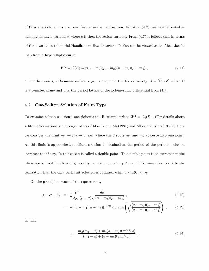
of W is aperiodic and is discussed further in the next section. Equation (4.7) can be interpreted as

defining an angle variable θ where c is then the action variable. From (4.7) it follows that in terms

of these variables the initial Hamiltonian flow linearizes. It also can be viewed as an Abel -Jacobi

map from a hyperelliptic curve

W 2 = C(E) = 2(µ−m1)(µ−m2)(µ−m3)(µ−m4) , (4.11)

or in other words, a Riemann surface of genus one, onto the Jacobi variety: J = [C|wZ] where C

is a complex plane and w is the period lattice of the holomorphic differential from (4.7).

4.2 One-Soliton Solution of Kaup Type

To examine soliton solutions, one deforms the Riemann surface W 2 = C4(E). (For details about

soliton deformations see amongst others Ablowitz and Ma(1981) and Alber and Alber(1985).) Here

we consider the limit m1 → m2 → a, i.e. where the 2 roots m1 and m2 coalesce into one point.

As this limit is approached, a soliton solution is obtained as the period of the periodic solution

increases to infinity. In this case a is called a double point. This double point is an attractor in the

phase space. Without loss of generality, we assume a < m3 < m4. This assumption leads to the

realization that the only pertinent solution is obtained when a < µ(0) < m3.

On the principle branch of the square root,

x− ct+ θ0 =1

2

∫ µ

µ0

dµ

(µ− a)√

(µ−m3)(µ−m4), (4.12)

= − [(a−m4)(a−m3)]−1/2 arctanh

(√

(a−m4)(µ−m3)

(a−m3)(µ−m4)

)

, (4.13)

so that

µ =m3(m4 − a) +m4(a−m3)tanh2(ω)

(m4 − a) + (a−m3)tanh2(ω), (4.14)

15

where ω = −(x − ct + θ0)√

(a−m4)(a−m3) and a,m3,m4 are functions of c. Using the trace

formulas (3.12)-(3.13) and the transformations (A.3)-(A.4), the exact formulas for U and W from

the Boussinesq equation are obtained. For example,

U =−4a2 + (m3 −m4)

2 + 2a(m3 +m4) + (m24 −m2

3)cosh(2ω)

2a− (m3 +m4) + (m3 −m4)cosh(2ω). (4.15)

Notice that µ has a shape similar to a KdV solitary wave. It has a peak at m3 and approaches

m1 for large |x|. From this we conclude that U is also shaped like a KdV soliton with a peak of

height 4a+ 2m4 − 2m3 and for large |x| approaches 2m3 + 2m4. One might be surprised that the

soliton does not approach 0 as x → ±∞. But remember that this is the modified cKdV equation

with K1 6= 0. Howver we may choose the parameters so that the solution does approach zero. The

solution is plotted in Figure B.2. This solution was first found by Kaup(1972) using the inverse

scattering transform in case when m3 = −m4 and a = 0, hence K1 = 0. One advantage of the

approach used here is that W is easily found using the trace formulas, and the relationship between

U and W is seen explicitly.

4.3 Solutions with Two Peaks.

Observe next that since n = 1, W is only a quadratic in U . The polynomial

W = −12U

2 + (2a+m3 +m4)U − 4am3 − 4am4 + (m3 −m4)2 , (4.16)

obtained from the trace formula is a parabola in U with vertex at U = 2a+m3 +m4. Since U has

the shape of a solitary wave, W has either one or two peaks depending on the parameters defining

the vertex of U . (See Figure B.2). If U is concave down, then W is a double peaked soliton if

m3 +m4 < 2a and 3m3 < 2a +m4. In the unperturbed case (γ = 0), these conditions reduce to

m3 < 0 < a. Otherwise W has a single peak. The concave up case is similar.

16

4.4 One Kink Solution

The one-kink solutions were initially found by Alonso and Rues(1992) as the simplest solutions

obtained using the bilinear formalism of the Kyoto school. Our method introduces an alternate

description of soliton fusion and fission for n = 2 and simplifies the computations.

To obtain the one-kink solutions, we deform the Riemann surface further by taking the limit

m3 → m4, so that m1 = m2 = a1 and m3 = m4 = a2. Note that if κ = −1 this limit is not

permitted for real valued µ in (3.7). However, for κ = 1 the system is readily solved for real µ

producing a special case of equation (4.5) where τ1 = 0 = τ2 = γ. After inverting, the angle variable

is

θ = x− ct+ θ0 = ±∫

2dU

U(U − 2c)= ∓2

carctanh

(

U − c

c

)

, (4.17)

and we find using the trace formulas and the transformations obtained in Appendix A that

U = ±c tanh(− c2(x− ct+ θ0)) + c2 , (4.18)

W = ±c2

2sech2(− c

2(x− ct+ θ0)) . (4.19)

These functions are plotted in Figure B.3. Here U is always a kink or anti-kink while W is always

similar to a typical KdV soliton. Observe that the speed of the soliton, c2/2 is exactly the amplitude

of W and is proportional to the square of the amplitude of the U soliton. This connection between

wave speed and amplitude is reminiscent of that found in the KdV equation.

5 Classification of Limits of Genus-Two Solutions

In this section genus-two quasi-periodic solutions are constructed. By deforming the Riemann

surface (spectral polynomial), two-soliton solutions are obtained and several types of soliton-soliton

interactions are described.

17

5.1 Quasi-periodic Genus-Two Solutions

In the genus-two case U is given by the trace formulas to be the sum of two periodic functions,

µ1 and µ2, and a constant. In general the functions, µ1 and µ2, have noncommensurate periods,

so that the solution U is generically quasi-periodic and systems (3.7) and (3.8) are defined on the

symmetric product of two copies of the Riemann surface (hyperelliptic curve) of genus two given

by

W 2 = C6(E) , (5.1)

where

C6(E) = κ

6∏

l=1

(E −mj) . (5.2)

After reordering the equations, summing them up, and integrating, the following Jacobi inversion

problem is obtained:

θ1 =

∫ µ1

µ0

1

dµ1√

C6(µ1)+

∫ µ2

µ0

2

dµ2√

C6(µ2)= 2x− 2a1t+ θ0

1 , (5.3)

θ2 =

∫ µ1

µ0

1

µ1dµ1√

C6(µ1)+

∫ µ2

µ0

2

µ2dµ2√

C6(µ2)= 2x− 2a2t+ θ0

2 . (5.4)

Inverting the Abel-Jacobi map defined by (5.3)-(5.4) results in expressions for µ1 and µ2 in terms

of Riemann θ-functions. (For details about the Abel-Jacobi map see Mumford(1983), Matveev and

Yavor(1979), and Ercolani and McKean (1990).)

Having derived the genus-two quasi-periodic solutions, several limiting cases will now be ex-

plored to introduce solitons. Below each distinct case is considered.

5.2 One-Soliton Solution on a Quasi-periodic Background

A one-soliton solution on a quasi-periodic background is obtained in the limit m1 → m2 → a. Just

as in the one-soliton case, a soliton is created as the Riemann surface is manipulated by pinching

18

two elements of the spectrum. However, in this case there are two µ variables and the orbit for only

one µ-variable is changed. The other µ variable remains periodic. The result is a solution with a

Kaup type soliton on a quasi-periodic background, and it is plotted in Figure B.4. The problem of

inversion may be written in the following way,

θ1 =

∫ µ1

µ0

1

dµ1

(µ1 − a)√

P4(µ1)+

∫ µ2

µ0

2

dµ2

(µ2 − a)√

P4(µ2)= 2t+ θ0

1 , (5.5)

θ2 =

∫ µ1

µ0

1

dµ1√

P4(µ1)+

∫ µ2

µ0

2

dµ2√

P4(µ2)= 2x− 2at+ θ0

2 , (5.6)

where

P4(E) = (E −m3)(E −m4)(E −m5)(E −m6) . (5.7)

(For details about inverting problems of this type see Alber and Fedorov(1999).)

5.3 Two-Soliton Solutions of Kaup Type

The two-soliton solution is obtained by piecewise pinching together two pairs of elements of the

spectrum so that m1 → m2 → a1 and m3 → m4 → a2. Here there are two double points a1

and a2, as well as two remaining hyperelliptic points at m5 and m6. Choosing the initial data on

the positive branch of the Riemann surface for both µ variables leads to the following problem of

inversion

θ1 =

∫ µ1

µ0

1

dµ1

(µ1 − a2)√

(µ1 −m5)(µ1 −m6)

+

∫ µ2

µ0

2

dµ2

(µ2 − a2)√

(µ2 −m5)(µ2 −m6)= 2x− 2a1t+ θ0

1 , (5.8)

θ2 =

∫ µ1

µ0

1

dµ1

(µ1 − a1)√

(µ1 −m5)(µ1 −m6)

+

∫ µ2

µ0

2

dµ2

(µ2 − a1)√

(µ2 −m5)(µ2 −m6)= 2x− 2a2t+ θ0

2 . (5.9)

This angle representation is similar to the one found in the case of the defocusing NLS equation.

(See Alber and Marsden(1994).)

19

Notice that the θi’s are essentially the sum of two Kaup type solitons as t → ±∞. The

integrals in system (5.8),(5.9) may be evaluated to obtain the following nonlinear algebraic system

of equations for the µi:

(s1625 + s1526)(s2625 + s2526) = A1(s1625 − s1526)(s2625 − s2526) , (5.10)

(s1615 + s1516)(s2615 + s2516) = A2(s1615 − s1516)(s2615 − s1516) , (5.11)

where sijkl =√

(µi −mj)(ak −ml) and

A1 = exp[−√

(a2 −m5)(a2 −m6)(2x− 2a1t+ θ01)] , (5.12)

A2 = exp[−√

(a1 −m5)(a1 −m6)(2x− 2a2t+ θ02)] . (5.13)

5.4 Phase Shift Formulas

When two solitons interact, they normally re-emerge with their initial profile and velocity. However,

they have shifted ahead or behind where they would have been had there been no interaction at

all. The amount a soliton shifts is called its phase shift, and the integral equations (5.8),(5.9) can

be used to compute it. Assume that a1 > a2 and define

M(x) =

√

x−m5

x−m6. (5.14)

The phase shifts for the systems (5.8)-(5.9) are calculated by using the following procedure. First,

consider the reference frame where θ1 is a constant, that is 2x− 2a1t+ θ01 = α1 for some constant

α1. Then observe that θ2 can be written only as a function of t and α1. Namely, θ2 = α1 + 2(a1 −

a2)t+ θ02 − θ0

1. Notice that the integrals on the left hand side of (5.8) are exactly the expression for

single Kaup type solitons. Integrals of this form may be integrated as

∫ µ2

µ0

2

dµ2

2(µ2 − a1)√

(µ2 −m5)(µ2 −m6)=

1

2√

(a1 −m5)(a1 −m6)log

∣

∣

∣

∣

ψ −M(a1)

ψ +M(a1)

∣

∣

∣

∣

, (5.15)

20

where for clarity we have defined ψ2 = M(µ2)2. Then we see that in this frame when t → ∞ the

right side of (5.9) goes to infinity so that the left hand side must also grow without bound. On

evaluation of the integrals we see that this can only happen when ψ → −M(a1). Similarly when

t → −∞, ψ must approach M(a1). Substituting these values for µ2 in (5.9) gives asymptotics for

θ1 as t → ∞ and as t → −∞, respectively. The phase shift for one of the solitons will be the

difference between the behavior of θ1 at minus infinity and its behavior at plus infinity in the frame

given by θ1 = α1. In this way we obtain the shift between phases before and after interaction for

θ1 to be

∆1 =1

√

(a2 −m5)(a2 −m6)log

∣

∣

∣

∣

M(a2) +M(a1)

M(a2) −M(a1)

∣

∣

∣

∣

. (5.16)

Similarly the phase shift for µ2 along θ2 = α2 is computed to be

∆2 =1

√

(a1 −m5)(a1 −m6)log

∣

∣

∣

∣

M(a1) +M(a2)

M(a1) −M(a2)

∣

∣

∣

∣

. (5.17)

These formulas were initially obtained by Matveev and Yavor(1979) by studying asymptotics of

singular θ-functions.

5.5 Kink-Anitkink Interaction Solutions

The interaction of kink and antikink solutions will now be considered. The two-kink solutions are

constructed by taking the limit of the spectral parameters so that m1 → m2 → a1, m3 → m4 → a2,

and m5 → m6 → a3. We examine both the case when the µi’s are both initially on the positive

branch of the Riemann surface and the case when only one of the µi’s is initially on the positive

branch and the other is on the negative branch. In contrast to the KdV equation, this difference

in the initial conditions produces qualitatively different solutions. This difference arises because

the KdV and cKdV equations contain at least one hyperelliptic branch point, while all of the fixed

points are double points for the two-kink solutions.

21

5.6 Initial values of µ1 and µ2 are chosen on the positive branches of the Rie-

mann surface.

In this situation, the angle variables are computed to be

θ1 = +

∫ µ1

µ0

1

dµ1

(µ1 − a2)(µ1 − a3)

+

∫ µ2

µ0

2

dµ2

(µ2 − a2)(µ2 − a3)= 2x− 2a1t+ θ0

1 , (5.18)

θ2 = +

∫ µ1

µ0

1

dµ1

(µ1 − a1)(µ1 − a3)

+

∫ µ2

µ0

2

dµ2

(µ2 − a1)(µ2 − a3)= 2x− 2a2t+ θ0

2 . (5.19)

These integrals are tractable, and the symmetric polynomials µ1µ2 and µ1 + µ2 which appear in

the trace formulas, can be calculated explicitly from the resulting system

(1 −A1)µ1µ2 + (a3A1 − a2)(µ1 + µ2) = A1a23 − a2

2 , (5.20)

(1 −A2)µ1µ2 + (a3A2 − a1)(µ1 + µ2) = A2a23 − a2

1 , (5.21)

with

A1 =(µ0

1 − a2)(µ02 − a2)

(µ01 − a3)(µ0

2 − a3)e2(a2−a3)(x−a1t+θ0

1) , (5.22)

A2 =(µ0

1 − a1)(µ02 − a1)

(µ01 − a3)(µ

02 − a3)

e2(a1−a3)(x−a2t+θ0

1) . (5.23)

These calculations are carried out for the unperturbed Boussinesq equations (K1 = 0) in the next

section and soliton fusion and fission are discussed.

5.7 Soliton Fusion and Fission.

Given this particular deformation of the Riemann surface, solitons can undergo fission or fusion.

This interesting phenomenon occurs when two separate solitons enter an interaction but only one

single soliton emerges from this interaction. Since all of the equations under study are invariant

22

under the space-time inversion (x → −x, t → −t), the reverse process of soliton fission may also

occur where a single soliton breaks into two distinct solitons at some critical time. Observe that

soliton fission can be interpreted as an infinite phase shift. This is because the solitons change their

speed since when they fuse together. Therefore they will be infinitely far from where they would

have been had there been no interaction. In this sense formulas (5.16)-(5.17) are still correct since

in the limit m5 = m6 = a3, M(x) = 1 and so the formulas become singular.

For this discussion we assume that γ = −2∑2n+2

i=1 mi = 0 although the general case is similar.

Hence the system (5.20)-(5.21) can be solved for µ1 + µ2 and is found to be

U = −4(µ1 + µ2) = −4a1f1 + a2f2 + a3f3

f1 + f2 + f3, (5.24)

where

f1 = exp(2a1x+ 2a21t+ θ1) , (5.25)

f2 = exp(2a2x+ 2a22t+ θ2) , (5.26)

f3 = exp(2a3x+ 2a23t+ θ3) , (5.27)

and

θ1 = a1θ01 + log [(a2 − a3)(µ

01 − a1)(µ

02 − a1)] , (5.28)

θ2 = a2θ01 + log [(a3 − a1)(µ

01 − a2)(µ

02 − a2)] , (5.29)

θ3 = a3θ02 + log [(a1 − a2)(µ

01 − a3)(µ

02 − a3)] . (5.30)

The expression (5.24) coincides with a solution to Burger’s equation which describes a confluence

of shocks (see Whitham(1974)) and has the same form as a solution obtained by using the Hirota

method. This expression is now analyzed to see why it represents soliton fusion. Suppose a1 <

0 < a2 < a3 and consider t = 0. We claim that at this instant (5.24) is a two-tiered kink (sum of

two kinks), see Figure B.8. To see why this is the case, consider 2x < (θ2 − θ1)/(a1 − a2). For

23

these values of x, f1 is the largest of the terms f1, f2, and f3. In fact as x → −∞, the terms

f2,f3 are negligible in comparison to f1. So for these values of x, µ1 + µ2 is nearly constant and is

approximately a1. Similarly for (θ2 − θ1)/(a1 − a2) < 2x < (θ3 − θ2)/(a2 − a3), f2 is the dominant

term and µ1 + µ2 ≈ a2. For the remaining values of x, f3 dominates so µ1 + µ2 ≈ a3.

We now apply this analysis for arbitrary t. In this manner we get that U is essentially constant

in three regions, D1, D2 and D3, of the (x, t) plane as seen in Figure B.7. When t is sufficiently

small, these regions are bounded by the points where the functions f1 = f2 and where f2 = f3. At

t∗ =(a2 − a3)(θ2 − θ1) − (a1 − a2)(θ3 − θ2)

2(a1 − a2)(a2 − a3)(a1 − a3), (5.31)

the functions f1 = f2 = f3 for some x∗. From this instant on, f2 is never the largest term and so

for t > t∗, the plane is divided into two regions bounded by the points where f1 = f3 as seen in

Figure B.7. For more details on this analysis see Whitham’s(1974) chapter on Burger’s equation.

As explained above, the regions Di, which contain all the information regarding fission of the

two-kink solution (times, speeds etc.), are derived from the parameterization of the lines f1 = f2,

f2 = f3, and f1 = f3. These lines are computed explicitly giving that f1 = f2 along the line where

2x = 2a3t+ (θ2 − θ1)/(a1 − a2), f2 = f3 along the line where 2x = 2a1t+ (θ3 − θ2)/(a2 − a3) and

f1 = f3 along the lines where 2x = 2a2t + (θ3 − θ1)/(a1 − a3). From this it is possible to predict

the times at which two solitons experience fission or fusion based solely on the initial phase and

the values of the three spectrum points ai. The speeds of the solitons are given by the slopes of

the lines, and in this way a complete explanation of fission is given. Notice that the arguments are

quite general and that this approach can be applied directly to the entire class of N -component

systems.

24

5.8 Initial values of µ1 and µ2 are chosen on different branches of the Riemann

surface.

This case gives a similar problem of inversion as the fusion case, namely

θ1 = +

∫ µ1

µ0

1

dµ1

(µ1 − a2)(µ1 − a3)

−∫ µ2

µ0

2

dµ2

(µ2 − a2)(µ2 − a3)= 2x− 2a1t+ θ0

1 , (5.32)

θ2 = +

∫ µ1

µ0

1

dµ1

(µ1 − a1)(µ1 − a3)

−∫ µ2

µ0

2

dµ2

(µ2 − a1)(µ2 − a3)= 2x− 2a2t+ θ0

2 . (5.33)

These integrals may be evaluated in terms of the log function and give rise to the following algebraic

equations for the µi’s

(µ1 − a1)(µ2 − a3)

(µ1 − a3)(µ2 − a1)=

(µ01 − a1)(µ

02 − a3)

(µ01 − a3)(µ

02 − a1)

exp[(a1 − a3)(2x− 2a2t+ θ02)] , (5.34)

(µ1 − a2)(µ2 − a3)

(µ1 − a3)(µ2 − a2)=

(µ01 − a2)(µ

02 − a3)

(µ01 − a3)(µ0

2 − a2)exp[(a2 − a3)(2x− 2a1t+ θ0

1)] . (5.35)

This is a system from which the µi’s can be found explicitly. The solutions are plotted in Figure B.9

and the corresponding U andW are graphed in Figure B.10. By initially choosing different branches

of this particular Riemann surface we see that the solitons ‘change form’, i.e. a kink changes

to an antikink and vice versa. An analytic explanation is given in the next section. This was

first observed in Alonso and Rues(1992) who noticed this phenomenon asymptotically. Using the

algebraic geometric construction the finite-time interactions can be analyzed as well.

5.9 Change of Form of Kinks to Antikinks.

The solutions obtained from (5.34) can be put in the following form

µ1 =−a1g1 − a2g2 − a3g3

g1 + g2 + g3, (5.36)

µ2 =a1h1 + a2h2 + a3h3

h1 + h2 + h3, (5.37)

25

where

g1 = exp

[

−2a1x− 2a2a3t− a1θ02 + log

(a3 − a2)(µ01 − a1)

µ02 − a1

]

, (5.38)

g2 = exp

[

−2a2x− 2a1a3t− a2θ01 + log

(a1 − a3)(µ01 − a2)

µ02 − a2

]

, (5.39)

g3 = exp

[

−2a3x− 2a1a2t− a3(θ01 + θ0

2) + log(a2 − a1)(µ

01 − a3)

µ02 − a3

]

, (5.40)

h1 = exp

[

2a1x+ 2a2a3t+ a1θ02 + log

(a3 − a2)(µ01 − a1)

µ02 − a1

]

, (5.41)

h2 = exp

[

2a2x+ 2a1a3t+ a2θ01 + log

(a1 − a3)(µ01 − a2)

µ02 − a2

]

, (5.42)

h3 = exp

[

2a3x+ 2a1a2t+ a3(θ01 + θ0

2) + log(a2 − a1)(µ

01 − a3)

µ02 − a3

]

. (5.43)

Notice the similarity between the form of the solutions (5.36),(5.37) and the solution (5.24) for U in

the previous case. Since they have an identical form as that in (5.24), all the analysis from the last

section applies and we conclude that both µ1 and µ2 are kinks which experience fission or fusion

respectively. We find that as t → −∞, µ1 is an antikink and µ2 decomposes into two kinks. This

implies that −14U = µ1 + µ2 consists of two kinks and one antikink. As t → ∞, µ1 fissions into

two antikinks and the 2 kinks comprising µ2 fuse into one kink. Therefore µ1 + µ2 is the sum of

one kink and two antikinks. This explains the transformation of kinks to antikinks and vice versa.

See Figure B.11 to see how these µ variables combine to form U . Of course the same analysis can

be performed as above to see this analytically. This is the first time two-soliton solutions of this

equation have been derived in this simple form.

6 The SHG Equations

Solutions of the cKdV may also be transformed into solutions of the SHG equation if κ is chosen

to be −1. This is shown explicitly in Appendix A. The results from the previous sections can be

viewed in the context of the SHG equations. First, if κ = −1, the initial conditions must be chosen

26

differently or the µi’s will not be real valued. That is, the cases κ = 1 and κ = −1 are dual to each

other in the sense that in the process of the construction of the Riemann surface the cuts in the

complex plane for the κ = 1 case correspond to where real valued solutions lie in the κ = −1 case

and vice versa. This is because the kappa appears under the square root in (3.7) so that real values

of µ for kappa = 1 correspond exactly to imaginary values of µ when κ = −1 and vice versa.

Another important difference is that no kink solutions exist for the SHG equations. When

κ = −1 there is no way to deform the Riemann surface so that all points coalesce piecewise as

required for kink solitons. Therefore there are always at least two hyperelliptic points left. This

means that SHG solutions do not have a possibility of either fusing or fissioning and no change of

form can occur.

The phase shift formulas for this system are very similar to those in the cKdV hierarchy with

κ = 1, namely

∆1 =1

√

−(a2 −m5)(a2 −m6)log

∣

∣

∣

∣

M(a2) +M(a1)

M(a2) −M(a1)

∣

∣

∣

∣

, (6.1)

∆2 =1

√

−(a1 −m5)(a1 −m6)log

∣

∣

∣

∣

M(a1) +M(a2)

M(a1) −M(a2)

∣

∣

∣

∣

. (6.2)

This is the first time these formulas have been derived. It is remarkable that the formulas are so

similar to those of the coupled KdV equation since they are not in the same hierarchy of equations -

the two equations are derived from two different potentials. The phase shift formulas show another

strength of the algebraic geometric method since the details of the inverse scattering transform

have not been completed at this time, see Khusnutdinova(1998). u and v are plotted in Figure

B.12. These functions can be transformed into q1, q2 of the SHG by transformations in Appendix

A.

7 Modified Coupled Dym Equations

27

7.1 Genus-1 solutions for the cDym System

7.1.1 Periodic solutions.

A periodic solution of the cDym equation is described by the following differential equation

√µdµ

√

∏4i=1(µ−mi)

= dX , (7.1)

for particular choice of mi’s. Here X = 2x− 2ct+ θ0 and integration is carried out on the Riemann

surface W 2 =C(E)

E. This can be reduced to a standard form by introducing a new variable Y by

dY =dXõ. (7.2)

After integration (7.1) becomes

∫ µ

µ0

dµ√

∏4i=1(µ−mi)

= Y . (7.3)

Notice that this holomorphic differential is defined on a genus two Riemann surface. To invert this

integral one has first to consider the following problem of inversion

∫ µ1

µ0

1

dµ1√

µ1C4(µ1)+

∫ µ2

µ0

2

dµ2√

µ2C4(µ2)= θ0

1 , (7.4)

∫ µ1

µ0

1

µ1dµ1√

µ1C4(µ1)+

∫ µ2

µ0

2

µ2dµ2√

µ2C4(µ2)= X1 + θ0

2 , (7.5)

where C4(µ) =∏4

l=1(µ−mj). One needs to rearrange integrals in such a way that to obtain X1 on

the right hand side of the first integral equation. This yields exact formulas for µ1 and µ2 in terms

of Riemann θ-functions. By fixing µ2 = m3 and writing µ = µ1 we resolve the initial problem of

inversion. (For details see Alber and Fedorov(1999).)

28

7.1.2 Kink solutions.

Now consider a kink limit by setting m1,m2 → a1 and m3,m4 → a2 such that a2 > a1 > 0. Integral

(7.3) becomes

dµ

(µ− a1)(µ− a2)= dY . (7.6)

Observe that this is the same problem of inversion as in the cKdV case except that we have Y

instead of X on the right hand side. After integrating we obtain

µ(Y ) =a1(µ0 − a2) − a2(µ0 − a1) exp((a1 − a2)Y )

(µ0 − a2) − (µ0 − a1) exp((a1 − a2)Y ). (7.7)

This gives µ as a function of Y and as in the cKdV case this is a kink. X is defined in terms of

Y by (7.2) once we know µ(Y ) from (7.7). The integration in (7.2) may be carried out explicitly.

Note that dX/dY > 0 and so X(Y ) is always increasing. By the definition of X it is also clear

that the range of X(Y ) is all real numbers. Therefore the Inverse Function Theorem implies that

an inverse function Y = Y (X) exists for all values of X and is monotonically decreasing. Therefore

the graph of µ(X) = µ(Y (X)) will have a similar appearance to that of µ(Y ), that is, it is also a

kink.

After combining numerics for Y (X) with the expression for µ, a description for the kink of the

cDym system is obtained, see Figure B.13.

7.1.3 Cusp solution

For this solution, the limit m1,m2 → a1 and m3,m4 → a2 such that a2 < 0 < a1 is analyzed. The

analysis is the same as in the kink case except that now dX/dY changes sign exactly once when

the branch point Y ∗ is crossed where µ(Y ∗) = 0. In this case, Y (X) has two branches begining at

the hyperelliptic point X∗ where Y (X∗) = Y ∗. Therefore µ(X) has two branches and reaches a

cusp at the point X∗. See Figure B.14.

29

7.1.4 Peakon solution

If the Camassa-Holm shallow water equation is an indication(1994), a peakon may develop in the

limit m1,m2 → a1 and m3,m4 → a2 with a2 = 0 < a1. The analysis is similar to that of the kink

case, except now the range of X(Y ) is bounded above by some number X∗. This means that the

inverse function Y (X) is defined only for those X < X∗. But, it can be defined symmetrically, as

if the integration were carried out on the negative branch of the square root, and this gives rise to

a peakon solution. The difference between this and a cusp solution is that in the cusp,

dY

dX=

1õ, (7.8)

is infinite at the branch point, while in the Peakon case µ(Y ) > 0 for all Y and so at the branch

point the derivative is finite.

7.2 Genus 2 solutions

The algebraic geometric procedure outlined thus far in this paper can be used for other equations

as well, even when other methods may fail. (For details see Alber and Fedorov (1999).) Using our

experience with the cKdV system, the case when there are three double points will be considered.

For the positive branch of the Riemann Surface W 2 = C(E)/E, the problem of inversion can be

written as

µ1dµ1

2(µ1 − a1)(µ1 − a2)(µ1 − a3)√µ1

+µ2dµ2

2(µ2 − a1)(µ2 − a2)(µ2 − a3)√µ2

= dt , (7.9)

µ21dµ1

2(µ1 − a1)(µ1 − a2)(µ1 − a3)√µ1

+µ2

2dµ2

2(µ2 − a1)(µ2 − a2)(µ2 − a3)√µ2

= dx . (7.10)

This inversion problem is very similar to that in the cKdV case, with the exception of the poles

present in the left hand side of the equation. This case is complicated by the fact that only

differentials of the third kind appear having simple poles at a1, a2, a3. Following the procedure

30

outlined in Alber and Fedorov(1999), a third variable y is introduced such that

dµ1

2(µ1 − a1)(µ1 − a2)(µ1 − a3)√µ1

+dµ2

2(µ2 − a1)(µ2 − a2)(µ2 − a3)√µ2

= dy . (7.11)

Also the normalized differentials of the third kind are introduced

Ωi =αidµ

(µ− α2i )√µ, i = 1, 2, 3 , (7.12)

where αi =√ai. Next, consider three points zi given by

3∑

j=1

∫ Pj

P0

Ωi = zi , i = 1, 2, 3 . (7.13)

The zi are dependent on x, t, y by

z1 = 2√a1 [x− (a2 + a3)t+ a2a3y] , (7.14)

z2 = 2√a2 [x− (a1 + a3)t+ a1a3y] , (7.15)

z3 = 2√a3 [x− (a1 + a2)t+ a1a2y] . (7.16)

Integrating (7.13) and putting ξ =√µ gives

(ξ1 − αi)(ξ2 − αi)(ξ3 − αi)

(ξ1 + αi)(ξ2 + αi)(ξ3 + αi)= ezi , i = 1, 2, 3 . (7.17)

This gives the following system for the symmetric polynomials in ξ.

1 − ez1 −α1(1 + ez1) α21(1 − ez1)

1 − ez2 −α2(1 + ez2) α22(1 − ez2)

1 − ez3 −α3(1 + ez3) α23(1 − ez3)

ξ1ξ2ξ3

ξ1ξ2 + ξ2ξ3 + ξ1ξ3

ξ1 + ξ2 + ξ3

=

α31(1 + ez1)

α32(1 + ez2)

α33(1 + ez3)

(7.18)

¿From this, the expression µ1 + µ2 + µ3 = ξ21 + ξ22 + ξ23 may be found as a function of z1, z2, z3.

The determinant of the matrix in the system must be zero to obtain nonzero solutions. This added

equation gives µ3 in terms of µ1 and µ2. Then we can find µ1 + µ2 as a function of z1, z2. Then

this solution must be connected to the (x, t) variables by using (7.14).

31

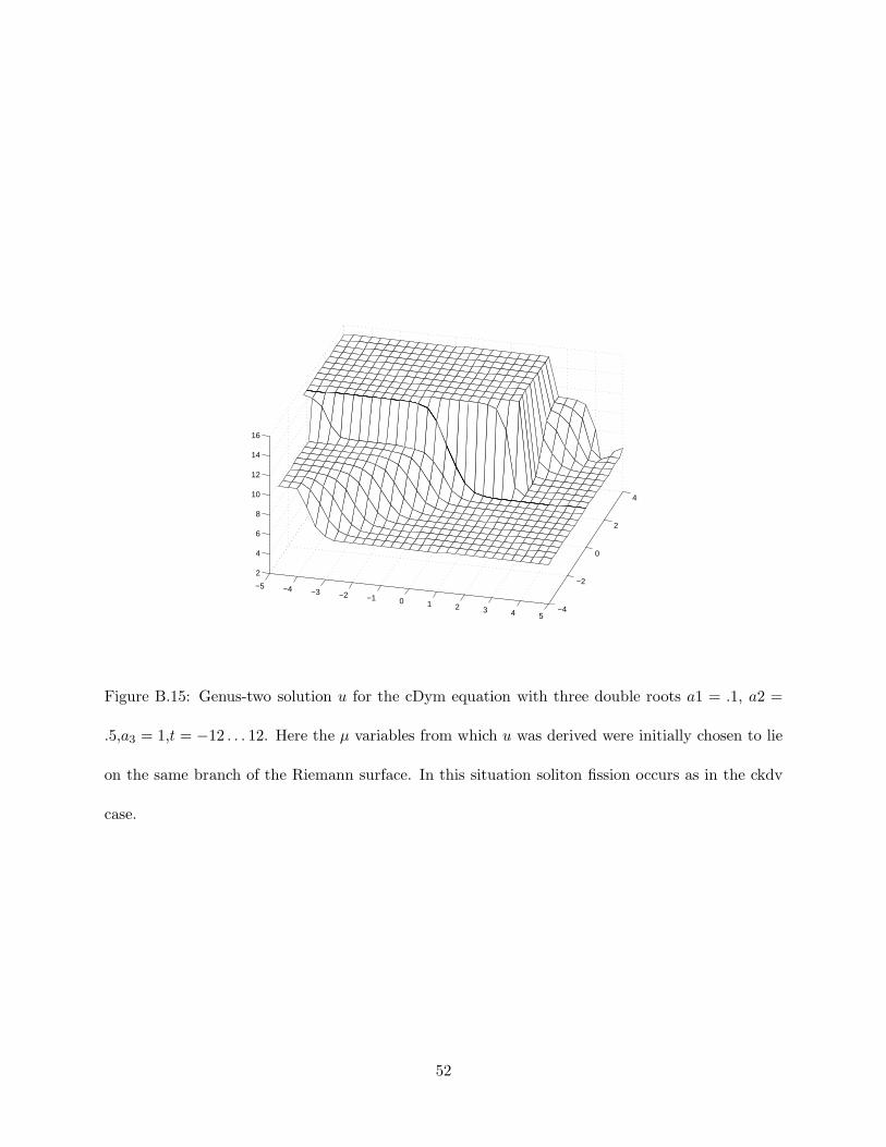
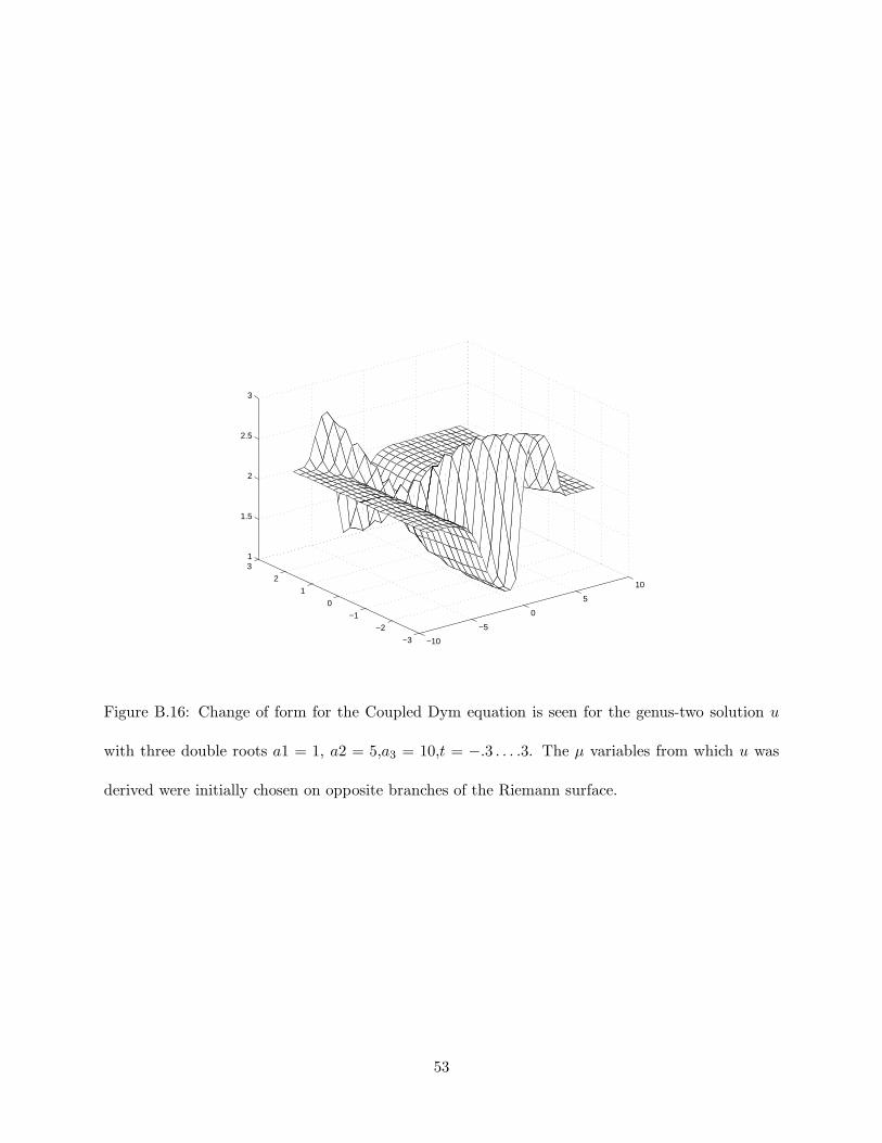
Numerics are provided in Figures B.15 and B.16. As expected, the phenomena of change of form

and fission occurs. A more detailed analysis of fission/fusion for the cDym case will be described

in a forth coming paper.

8 Acknowledgments

The research of Mark Alber and Gregory Luther was partially supported by NSF grant DMS

9626672. Mark Alber would like to thank Peter Miller for a helpful discussion and bringing to his

attention references Estevez et al.(1994) and Martinez Alonso and Medina Reus(1992).

A Transformations to Related Equations

In what follows we describe exact connections between solutions of the cKdV and the Kaup equa-

tions, Boussinesq systems and SHG system.

A.1 Generalized Coupled KdV System

For this system, assume that κ = 1 and r = 0. Observe that if we take n = 1, B takes the form of

B = E + b1. Furthermore, as in (B.1) we see that b1 = −u/2 +K1. Collecting coefficients of order

1 and 0 respectively in (2.9) and substituting the value of b1 shows that u, v satisfy the modified

cKdV system

ut = v′ − 32uu

′ +K1u′ , (A.1)

vt = 14u

′′′ − vu′ − 12uv

′ +K1v′ . (A.2)

K1 is a small parameter. When K1 = 0 this is the cKdV.

32

A.2 Generalized Boussinesq System

To connect u and v to the classical Boussinesq system the following change of variables must be

made

u(x, t) = −12U(X,T ) , (A.3)

v(x, t) = 116U(X,T )2 − 1

4W (X,T ) , (A.4)

where X = x and T = −t/2. Plugging in u and v from (A.3)-(A.4) into (A.1)-(A.2) and defining

γ = −2K1 we see that U and W satisfy

UT +WX + UUX = γUX , (A.5)

WT + UXXX + (WU)X = γWX . (A.6)

Again γ is a small parameter. When γ = 0, we have exactly the Boussinesq System. Otherwise

the system gives rise to a generalization of the Boussinesq system. Such a transformation can be

found in Sattinger(1995) for example.

A.3 Generalized Kaup Equations

To connect U(X,T ) and W (X,T ) from above to π(x, t) and φ(x, t) from the Kaup equations

(1.7),(1.8) the following change of variables was suggested by Kaup(1972):

U(X,T ) =ǫ

βφx(x, t) , (A.7)

W (X,T ) = β−2[1 − ǫπ(x, t)] , (A.8)

where X = x, T = βt, β = δ√

3/√

1 − 3σ, and α = βγ. Then substituting this into (A.5)-(A.6)

gives

πt = φxx + 13(1 − 3σ)δ2φxxxx − ǫ(φxπ)x + απx , (A.9)

π = φt + 12ǫφ

2x − αφx , (A.10)

33

which is a perturbed Kaup equations and reduces identically to it when α = 0. Summarizing we see

that every solution of the coupled KdV system yields, using the transformations stated, a solution

of the Boussinesq and Kaup systems.

A.4 The SHG System

For the SHG system we choose κ = −1 in the potential (2.6), and define w, ν by the equations

u = w, and v = νx/2 + ν2/4. Then the generating equation (3.1) becomes

Ewt + 12νxt + 1

2ννt = −12Bxxx + 2BxwE +Bxνx + 1

2Bxν2

−2BxE2 +BwxE + 1

2Bνxx + 12Bννx . (A.11)

Now we choose B = b/E, that is we choose m = 1, n = −1, b = b−2. Then (A.11) becomes

Ewt + 12νxt + 1

2ννt = − 12E bxxx + 2bxw + 1

E bxνx + 12E bxν

2

−2bxE + bwx + 12E bνxx + 1

2E bννx . (A.12)

Collecting coefficients of E gives

b = −η2, (A.13)

where we define η by ηx = wt. Then collecting coefficients of orders zero and one respectively and

substituting in the value for b gives

12νxt + 1

2ννt = −ηxw − 12ηwx (A.14)

0 = 14ηxxx − 1

2ηxνx − 14ηxν

2 − 14ηνxx − 1

4ηννx . (A.15)

(A.15) may be integrated to get

(ηx)x = (ην)ν + ηνx +

∫

νx(ην − ηx)dx . (A.16)

34

Notice that this equation is satisfied when ηx = ην. Next we define the new function s by the

relation νt = s−1 − ηw. Then plugging this into (A.14) gives

−sx

s2− ηxw − ηwx +

ν

s− ηνw = −2ηxw − ηwx . (A.17)

Substituting ηx = ην and canceling like terms yields sx = sν. These two equations, along with the

two we defined will determine the SHG system. Summarizing, we have

ηx = ην = wt , (A.18)

νt = s−1 − ηw , (A.19)

sx = sν . (A.20)

Next define Q = s−1 and φt = η. This and ηx = wt implies that w = φx. Therefore (A.18) becomes

(Qφt)x = Qxφt +Qφxt ,

= −sx

s2η +

ηx

s,

=1

s(ηx − ην) = 0 , (A.21)

and

(lnQ)xt − φxφt = −(ln s)xt − ηw ,

= −(sx

s

)

t− ηw ,

= −νt − ηw ,

= −(s−1 − ηw) − ηw = −Q . (A.22)

Finally, substitute q1 = (√Q/2) exp[i(φ/2)] and the real and imaginary parts of the following

equation correspond to (A.21) and (A.22), so that

q1xtq∗1 − q∗1tq1x = −2(q1q

∗1)

2 . (A.23)

35

If we define q2 = −[(lnQ)x + iφx] exp(iφ)/4. Then q1 and q2 satisfy

q1x = −2q2q∗1 , (A.24)

q2t = q21 , (A.25)

which is exactly the SHG equation, and q1 and q2 are obtained from the µ variables through the

relation

φx = u , (A.26)

Q = exp

(

− ut∫

ut dx

)

. (A.27)

The above transformations were inspired by Khusnutdinova(1998). Summarizing the above

gives that solutions of the SHG system may be expressed as follows

q1 =1

2exp

(

1

2

∫

ut

(∫

ut dx

)−1

dx

)

exp

(

i

2

∫

u dx

)

, (A.28)

q2 =1

4

(

d2

dx2log

(∫

utdx

)

− iu

)

exp

(

i

∫

u dx

)

. (A.29)

Notice that the dependence on v is implicit by the fact that ν = ut

(∫

ut dx)−1

.

B Trace Formulas

B.1 cKdV System

In this section, the connection between u, v, and µ for cKdV is derived. This connection is called

the trace formula for this system. Collect coefficients of En−r+2 in (3.1) to see that 2κb′0 = 0 from

which we assume that b0 = 1. Now gather coefficients of order n− r + 1 to arrive at

b1 = − u

2κ+K1 , (B.1)

36

for some constant of integration K1. Next collect coefficients of order 2n − 2r + 1 in (3.2) to see,

along with (B.1), that

K1 = −1

2

2n+2∑

i=1

mi . (B.2)

(B.1) then yields the trace formula for u,

u = 2κ

n∑

i=1

µi − κ

2n+2∑

i=1

mi . (B.3)

Now we just need the trace formula for v. For this we collect coefficients of order n− r in (3.1)

to get

0 = 2κb′2 + 2b′1u+ b1u′ + v′ , (B.4)

which gives upon substitution of b1 from (B.1) that

v′ = −2κb′2 +3uu′

2κ−K1u

′ , (B.5)

or simply

v = −2κb2 +3u2

4κ−K1u+K2 , (B.6)

where K2 is some constant and K1 is the same as above. From the definition of B(E) we see that

b2 =∑

1≤i<j≤n

µiµj . (B.7)

All that remains is to find K2. To derive this we collect coefficients of order 2n − 2r in (3.2). To

simplify calculations let cn be the (2n− 2r)th coefficient of the polynomial C(E). Then we see that

2κ(2b2 + b21) + 2u(2b1) + 2v = cn , (B.8)

or after substitution of the value of b1 that

4κb2 −3u2

2κ+ 2uK1 + 2κK2

1 + 2v = cn . (B.9)

37

Now solving for K2 in (B.6) and substituting in v from (B.9),

K2 = v + 2κb2 −3u2

4κ+K1u , (B.10)

=

(

c22

− 2κb2 +3u2

4κ− uK1 − κK2

1

)

+ 2κb2 −3u2

4κ+K1u , (B.11)

=c22

− κK21 . (B.12)

Now from the definition of C(E) we see that

cn = 2κ∑

1≤i<j≤2n+2

mimj . (B.13)

B.2 cDym System

In an analogous manner, we derive the trace formulas for the cDym system. The derivation of the

trace formula for u is identical to the cKdV case so that

u = 2n∑

i=1

µi −2n+2∑

i=1

mi . (B.14)

Only the trace formula for v is different. For this we collect coefficients of order n− r in (3.3)

to get

0 = −b′′′1

2+ 2b′2 + 2b′1u+ b1u

′ + v′ , (B.15)

which, upon substitution of b1 from (B.1) and integrating, gives

v = −u′′

4− 2b2 +

3u2

4−K1u+K2 , (B.16)

where K2 is some constant and K1 is the same as in cKdV. From the definition of B(E) we see

that

b2 =∑

1≤i<j≤n

µiµj . (B.17)

38

All that remains is to find K2. To derive this we collect coefficients of order 2n − 2r − 1 in (3.4).

To simplify calculations let cn−1 be the (2n − 2r − 1)st coefficient of the polynomial C(E). Then

we see that

−b′′1 + 2(2b2 + b21) + 2u(2b1) + 2v = cn−1 , (B.18)

or after substitution of the value of b1 that

u′′

2+ 4b2 −

3u2

2+ 2uK1 + 2K2

1 + 2v = cn−1 . (B.19)

Now solving for K2 in (B.16) and substituting in v from (B.19) gives

K2 = v + 2b2 −3u2

4+K1u+

u′′

4, (B.20)

= (c22

− 2b2 +3u2

4− uK1 −K2

1 − u′′

4) + 2b2 −

3u2

4+K1u+

u′′

4, (B.21)

=cn−1

2−K2

1 . (B.22)

¿From the definition of C(E) we see that

cn−1 = 2∑

1≤i<j≤2n+2

mimj . (B.23)

39

Bibliography

D. Mumford, Tata Lectures on Theta I and II, Progress in Math.28 and 43, (Birkhauser, Boston

1983).

Ercolani, N. and H. McKean, “Geometry of KdV(4). Abel sums, Jacobi variety, and theta function

in the scattering case,” Invent. Math 99, 483-544 (1990).

Ablowitz, M.J. and Y-C. Ma, “The Periodic Cubic Schrodinger Equation,” Studies in Appl. Math.

65, 113–158 (1981).

Alber, M.S. and S.J. Alber, “ Hamiltonian formalism for finite-zone solutions of integrable equa-

tions,” C. R. Acad. Sci. Paris Sr. I Math. 301, 777–781 (1985).

Alber, M.S. and J.E. Marsden, “On Geometric Phases for Soliton Equations,” Comm. Math.

Phys. 149, 217–240 (1992).

Antonowicz, M. and A.P. Fordy, “A family of completely integrable multi-Hamiltonian systems”,

Phys. Lett. A 122, 95–99 (1987).

Antonowicz, M. and A.P. Fordy, “Coupled KdV equations with multi-Hamiltonian structures,”

Physica D 28, 345–357 (1987).

Antonowicz, M. and A.P. Fordy, “ Coupled Harry Dym equations with multi-Hamiltonian struc-

tures,” J. Phys. A 21, L269–L275 (1988).

Antonowicz, M. and A.P. Fordy, “ Factorization of energy dependent Schrodinger operators: Miura

maps and modified systems,” Comm. Math. Phys. 124, 465–486 (1989).

Alber, M.S., G.G. Luther, and J.E. Marsden, “ Energy Dependent Schrodinger Operators and

Complex Hamiltonian Systems on Riemann Surfaces,” Nonlinearity 10, 223–242 (1997).

40

Channell, P.J. and C. Scovel, “Symplectic integration of Hamiltonian systems,” Nonlinearity 3,

231–259 (1990).

Channell, P.J. and C. Scovel, “An introduction to symplectic integrators,” Fields Institute Com-

munications 10, 45–58 (1996).

Alber, M.S., R. Camassa, D.D. Holm and J.E. Marsden, “The geometry of peaked solitons and

billiard solutions of a class of integrable PDE’s,” Lett. Math. Phys. 32, 137–151 (1994).

Alber, M.S., R. Camassa, D.D. Holm and J.E. Marsden, “On Umbilic Geodesics and Soliton

Solutions of Nonlinear PDE’s,” Proc. Roy. Soc. London Ser. A 450, 677–692 (1995).

Alber, M.S., R. Camassa, Yu.N. Fedorov, D.D. Holm and J.E. Marsden, “The geometry of new

classes of weak billiard solutions of nonlinear PDE’s,” (preprint) (1999).

Alber, M.S. and Yu.N. Fedorov, “Algebraic Geometric Solutions for Nonlinear Evolution Equations

and Flows on the Nonlinear Subvarieties of Jacobians,” (preprint) (1999)

Whitham, G.B., Linear and Nonlinear Waves, (Pure and applied mathematics, John Wiley &

Sons, Inc. 1974).

Jaulent, M., “On an inverse scattering problem with an energy dependent potential,” Ann. Inst.

H. Poincare A 17, 363–372 (1972).

Jaulent, M. and C. Jean, “The inverse problem for the one-dimensional Schodinger operator with

an energy dependent potential,” Ann. Inst. H. Poincare A I, II25, 105–118, 119–137 (1976).

Kaup, D.J., “A Higher-Order Water-Wave Equation and the Method for Solving It,” Prog. Theor.

Phys. 54, 72–78, 396–408 (1975).

41

Matveev, V.B. and M.I. Yavor, “Solutions presque periodiques et a N -solitons de lequation hy-

drodynamique non lineaire de Kaup,” Ann. Inst. Henri Poincare: Sec. A 31, 25–41 (1979).

Sachs, R.L., “On the integrable variant of the Boussinesq system: Painleve property, rational

solutions, a related many-body system, and equivalence with the AKNS hierarchy,” Physica

D 30, 1–27 (1998).

Martinez Alonso, L. and E. Medina Reus, “Soliton interaction with change form in the classical

Boussinesq system,” Phys. Lett. A 167, 370–376 (1992).

Estevez, P.G., P.R. Gordoa, L. Martinez Alonso, and E. Medina Reus , “On the characterization

of a new soliton sector in the classical Boussinesq system,” Inverse Problems 10, L23–L27

(1994).

Khusnutdinova, K.R. and H. Steudel, “Second harmonic generation: Hamiltonian structures and

particular solutions,” J. Math. Phys. 39, 3754–3764 (1998).

Sattinger, David and Szmigielski, Jacek, “Energy dependent scattering theory,” Differential and

Integral Equations 8, 945–959 (1995).

Sattinger, David and Szmigielski, Jacek, “A Riemann Hilbert problem for an energy dependent

Schrodinger operator,” Inverse Problems 12, 1003–1025 (1996).

Ablowitz, M.J. and Segur, H. , Solitons and the Inverse Scattering Transform, (SIAM, Philadel-

phia, 1981).

Belokolos, E.D., A.I. Bobenko, V.Z. Enol’sii, A.R. Its, and V.B. Matveev, Algebro-Geometric

Approach to Nonlinear Integrable Equations, (Springer-Verlag series in Nonlinear Dynamics,

1994).

42

Ercolani, N. “Generalized Theta functions and homoclinic varieties,” Proc. Symp. Pure Appl.

Math. 49, 87–100 (1989).

Kupershmidt, B.A., “Mathematics of Dispersive Water Waves,” Commun. Math. Phys. 99,

51–73 (1985).

43

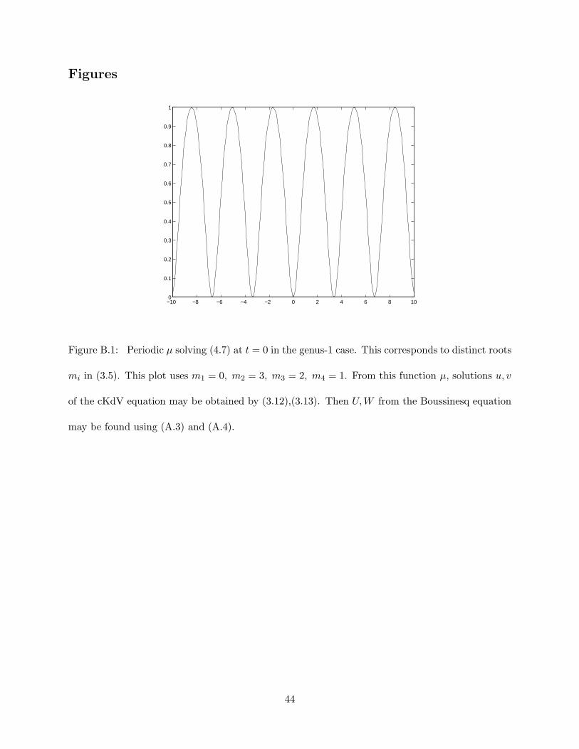
Figures

−10 −8 −6 −4 −2 0 2 4 6 8 100

0.1

0.2

0.3

0.4

0.5

0.6

0.7

0.8

0.9

1

Figure B.1: Periodic µ solving (4.7) at t = 0 in the genus-1 case. This corresponds to distinct roots

mi in (3.5). This plot uses m1 = 0, m2 = 3, m3 = 2, m4 = 1. From this function µ, solutions u, v

of the cKdV equation may be obtained by (3.12),(3.13). Then U,W from the Boussinesq equation

may be found using (A.3) and (A.4).

44

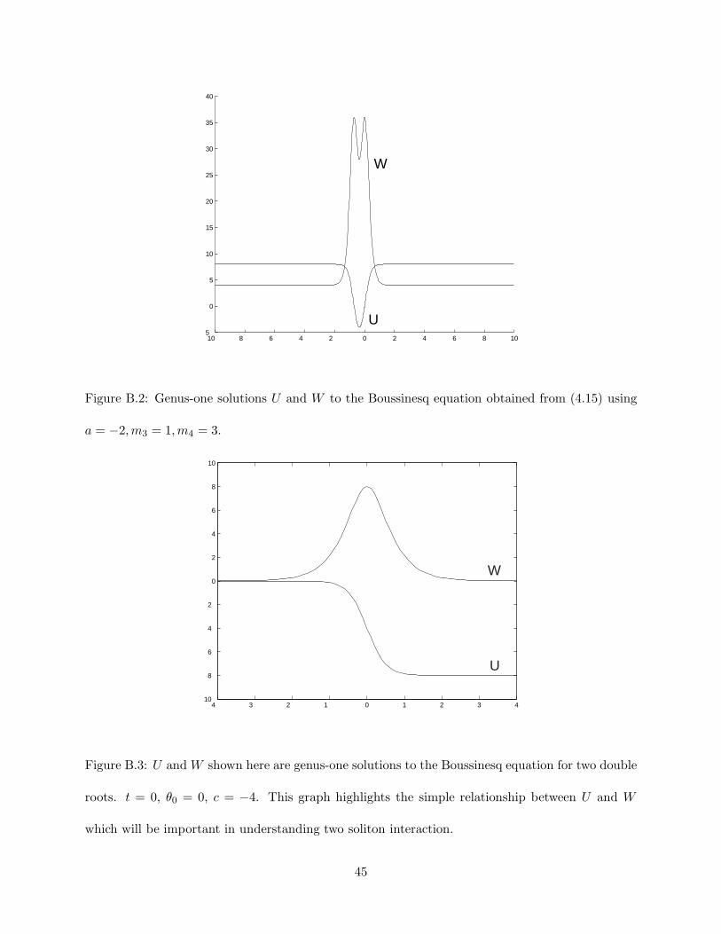
10 8 6 4 2 0 2 4 6 8 105

0

5

10

15

20

25

30

35

40

W

U

Figure B.2: Genus-one solutions U and W to the Boussinesq equation obtained from (4.15) using

a = −2,m3 = 1,m4 = 3.

4 3 2 1 0 1 2 3 410

8

6

4

2

0

2

4

6

8

10

W

U

Figure B.3: U and W shown here are genus-one solutions to the Boussinesq equation for two double

roots. t = 0, θ0 = 0, c = −4. This graph highlights the simple relationship between U and W

which will be important in understanding two soliton interaction.

45

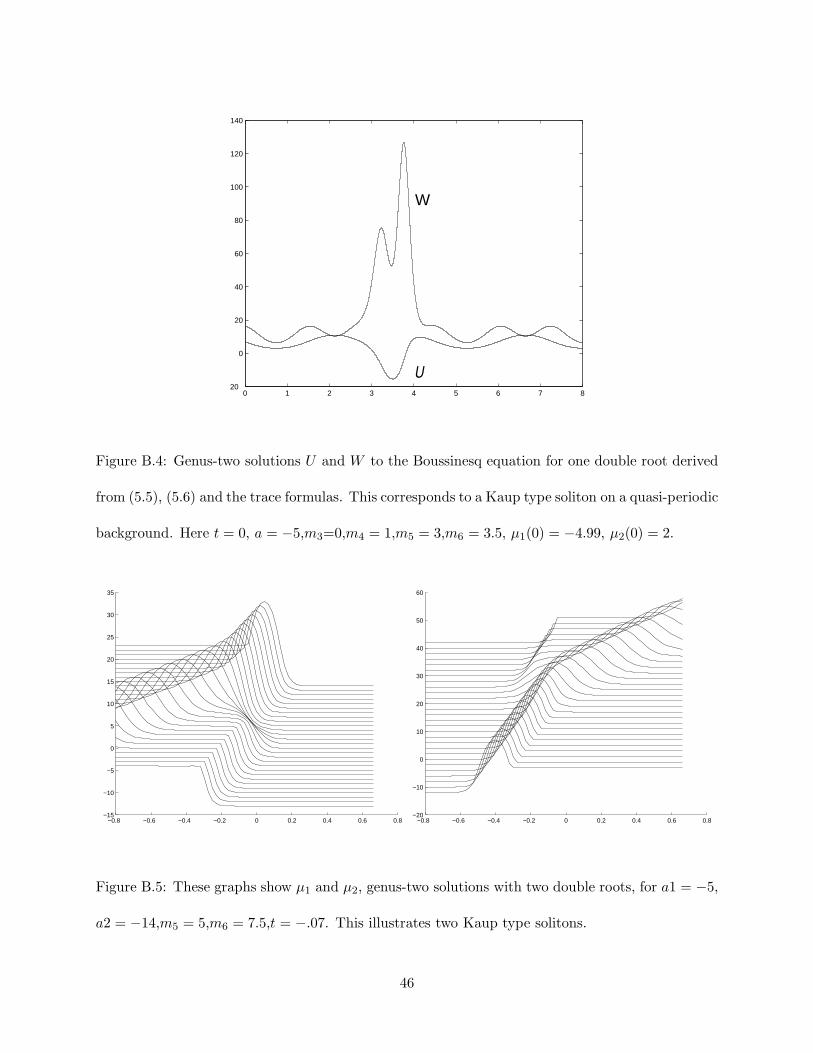
0 1 2 3 4 5 6 7 820

0

20

40

60

80

100

120

140

U

W

Figure B.4: Genus-two solutions U and W to the Boussinesq equation for one double root derived

from (5.5), (5.6) and the trace formulas. This corresponds to a Kaup type soliton on a quasi-periodic

background. Here t = 0, a = −5,m3=0,m4 = 1,m5 = 3,m6 = 3.5, µ1(0) = −4.99, µ2(0) = 2.

−0.8 −0.6 −0.4 −0.2 0 0.2 0.4 0.6 0.8−15

−10

−5

0

5

10

15

20

25

30

35

−0.8 −0.6 −0.4 −0.2 0 0.2 0.4 0.6 0.8−20

−10

0

10

20

30

40

50

60

Figure B.5: These graphs show µ1 and µ2, genus-two solutions with two double roots, for a1 = −5,

a2 = −14,m5 = 5,m6 = 7.5,t = −.07. This illustrates two Kaup type solitons.

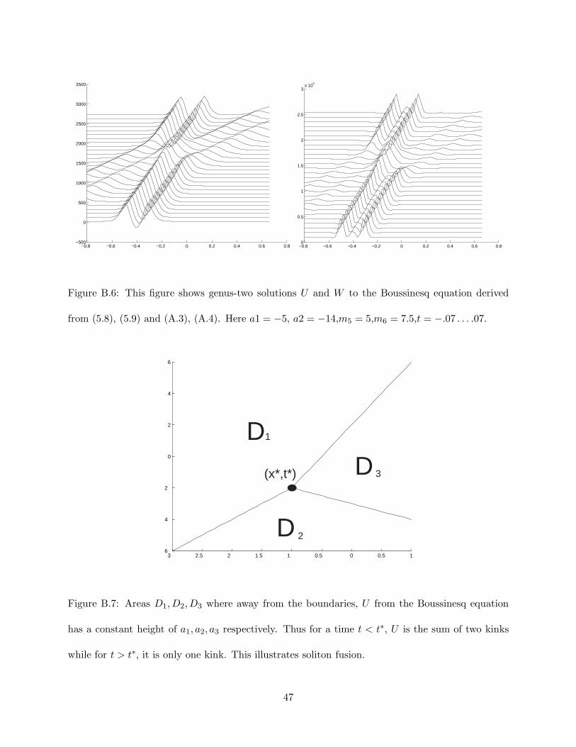
46

−0.8 −0.6 −0.4 −0.2 0 0.2 0.4 0.6 0.8−500

0

500

1000

1500

2000

2500

3000

3500

−0.8 −0.6 −0.4 −0.2 0 0.2 0.4 0.6 0.80

0.5

1

1.5

2

2.5

3x 10

5

Figure B.6: This figure shows genus-two solutions U and W to the Boussinesq equation derived

from (5.8), (5.9) and (A.3), (A.4). Here a1 = −5, a2 = −14,m5 = 5,m6 = 7.5,t = −.07 . . . .07.

3 2.5 2 1.5 1 0.5 0 0.5 16

4

2

0

2

4

6

a1

a2

a3

D1

D

D 2

3

(x*,t*)

Figure B.7: Areas D1,D2,D3 where away from the boundaries, U from the Boussinesq equation

has a constant height of a1, a2, a3 respectively. Thus for a time t < t∗, U is the sum of two kinks

while for t > t∗, it is only one kink. This illustrates soliton fusion.

47

−4 −3 −2 −1 0 1 2 3 4−10

0

10

20

30

40

50

60

−4 −3 −2 −1 0 1 2 3 40

20

40

60

80

100

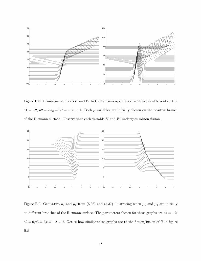
120

Figure B.8: Genus-two solutions U and W to the Boussinesq equation with two double roots. Here

a1 = −2, a2 = 2,a3 = 5,t = −.4 . . . .4. Both µ variables are initially chosen on the positive branch

of the Riemann surface. Observe that each variable U and W undergoes soliton fission.

−4 −3 −2 −1 0 1 2 3 4−5

0

5

10

15

20

25

−4 −3 −2 −1 0 1 2 3 4−5

0

5

10

15

20

25

Figure B.9: Genus-two µ1 and µ2 from (5.36) and (5.37) illustrating when µ1 and µ2 are initially

on different branches of the Riemann surface. The parameters chosen for these graphs are a1 = −2,

a2 = 0,a3 = 2,t = −2 . . . 2. Notice how similar these graphs are to the fission/fusion of U in figure

B.8

48

−4 −3 −2 −1 0 1 2 3 4−20

0

20

40

60

80

100

120

140

−4 −3 −2 −1 0 1 2 3 40

100

200

300

400

500

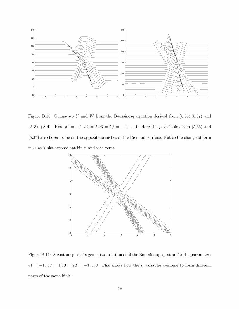
600

Figure B.10: Genus-two U and W from the Boussinesq equation derived from (5.36),(5.37) and

(A.3), (A.4). Here a1 = −2, a2 = 2,a3 = 5,t = −.4 . . . .4. Here the µ variables from (5.36) and

(5.37) are chosen to be on the opposite branches of the Riemann surface. Notice the change of form

in U as kinks become antikinks and vice versa.

−6 −4 −2 0 2 4 6−3

−2

−1

0

1

2

3

Figure B.11: A contour plot of a genus-two solution U of the Boussinesq equation for the parameters

a1 = −1, a2 = 1,a3 = 2,t = −3 . . . 3. This shows how the µ variables combine to form different

parts of the same kink.

49

3 2 1 0 1 2 315

10

5

0

5

10

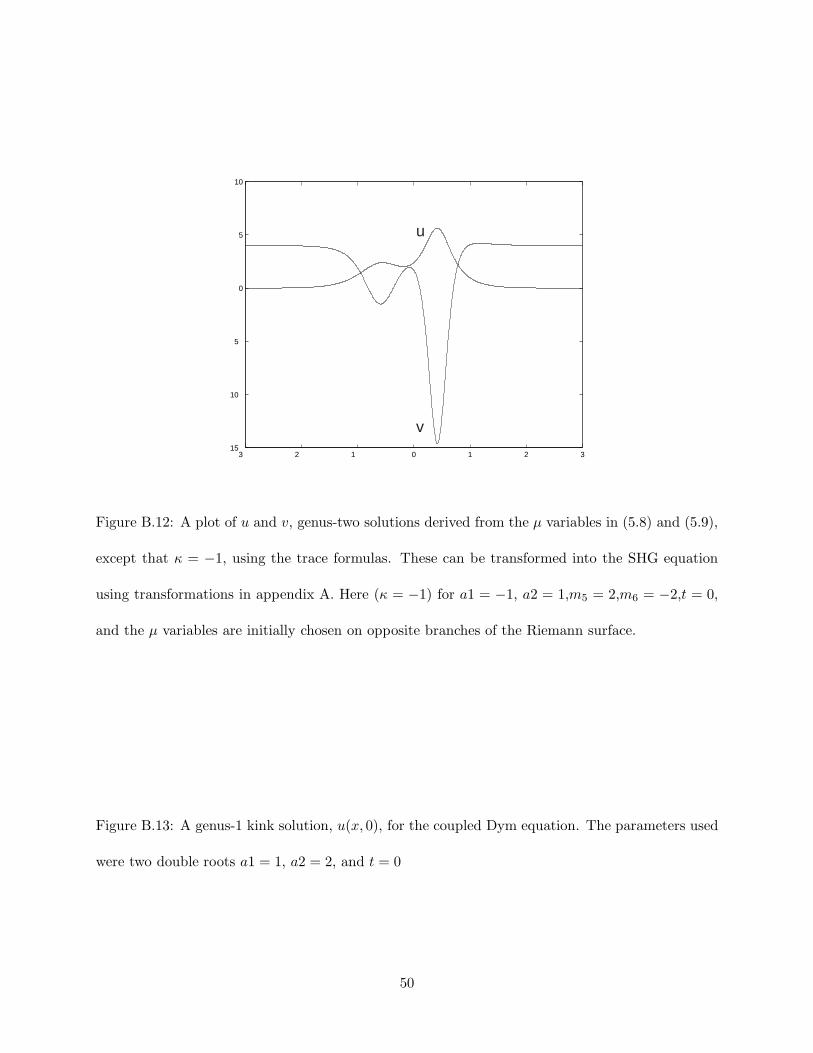
u

v

Figure B.12: A plot of u and v, genus-two solutions derived from the µ variables in (5.8) and (5.9),

except that κ = −1, using the trace formulas. These can be transformed into the SHG equation

using transformations in appendix A. Here (κ = −1) for a1 = −1, a2 = 1,m5 = 2,m6 = −2,t = 0,

and the µ variables are initially chosen on opposite branches of the Riemann surface.

Figure B.13: A genus-1 kink solution, u(x, 0), for the coupled Dym equation. The parameters used

were two double roots a1 = 1, a2 = 2, and t = 0

50

−5 −4 −3 −2 −1 0 1 2 3 4 5−0.5

0

0.5

1

1.5

2

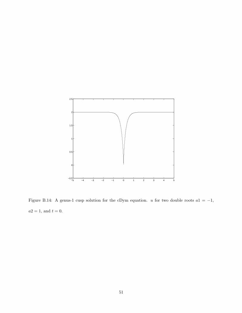
2.5

Figure B.14: A genus-1 cusp solution for the cDym equation. u for two double roots a1 = −1,

a2 = 1, and t = 0.

51

−5 −4 −3 −2 −1 0 1 2 3 4 5−4

−2

0

2

4

2

4

6

8

10

12

14

16

Figure B.15: Genus-two solution u for the cDym equation with three double roots a1 = .1, a2 =

.5,a3 = 1,t = −12 . . . 12. Here the µ variables from which u was derived were initially chosen to lie

on the same branch of the Riemann surface. In this situation soliton fission occurs as in the ckdv

case.

52

−10

−5

0

5

10

−3

−2

−1

0

1

2

31

1.5

2

2.5

3

Figure B.16: Change of form for the Coupled Dym equation is seen for the genus-two solution u

with three double roots a1 = 1, a2 = 5,a3 = 10,t = −.3 . . . .3. The µ variables from which u was

derived were initially chosen on opposite branches of the Riemann surface.

53