Soliton Interpretation of Arterial Blood Pressure Waveform
104
Delft Center for Systems and Control (DCSC) Biomechanical Engineering (BMechE) Soliton Interpretation of Arterial Blood Pressure Waveform: Derivation, Veri- fication of Korteweg-de Vries type Dy- namics and Application of Nonlinear Fourier Analysis G. Gezer Master of Science Thesis
-
Upload
khangminh22 -
Category
Documents
-
view
0 -
download
0
Transcript of Soliton Interpretation of Arterial Blood Pressure Waveform
Delft Center for Systems and Control (DCSC)Biomechanical Engineering (BMechE)
Soliton Interpretation of Arterial BloodPressure Waveform: Derivation, Veri-fication of Korteweg-de Vries type Dy-namics and Application of NonlinearFourier Analysis
G. Gezer
Mas
tero
fScie
nce
Thes
is


Soliton Interpretation of ArterialBlood Pressure Waveform: Derivation,Verification of Korteweg-de Vries type
Dynamics and Application ofNonlinear Fourier Analysis
Master of Science Thesis
For the degrees of Master of Science in Systems & Control andMechanical Engineering at Delft University of Technology
G. Gezer
January 21, 2019
Faculty of Mechanical, Maritime and Materials Engineering (3mE) · Delft University ofTechnology

Copyright c© Biomechanical Engineering and Delft Center for Systems and ControlAll rights reserved.

Delft University of TechnologyDepartment of
Biomechanical Engineering and Delft Center for Systems andControl
The undersigned hereby certify that they have read and recommend to the Faculty ofMechanical, Maritime and Materials Engineering (3mE) for acceptance a thesis
entitledSoliton Interpretation of Arterial Blood Pressure Waveform:
Derivation, Verification of Korteweg-de Vries type Dynamics andApplication of Nonlinear Fourier Analysis
byG. Gezer
in partial fulfillment of the requirements for the degrees ofMaster of Science Systems & Control and Mechanical Engineering
Dated: January 21, 2019
Supervisor(s):prof.dr.ir. J. Dankelman
dr.ir. S. Wahls
ir. P.J. Prins
Reader(s):prof.dr.ir. M. Verhaegen


Abstract
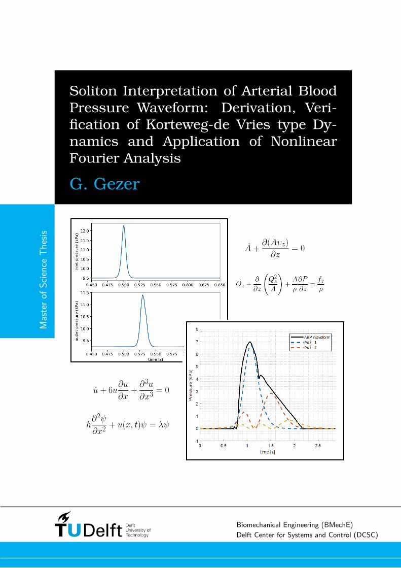
As a nonlinear alternative to the linear interpretation of arterial blood pressure waveform,soliton theory has been proposed to model arterial blood pressure by interpreting the pulsatilenature of pressure pulses in the viewpoint of soliton transmission. The existing solitary waveliterature supports this interpretation by deriving Korteweg-de Vries (KdV) type dynamicsfrom 1-D Navier-Stokes equations. In this paper, we explain and discuss the derivation ofKdV type dynamics for arterial blood pressure from basics of fluid motion. As original work,we provide two verification tests for two of the existing KdV models in three case studieswhich are considered to be interconnected sections of a simplified arterial network. Finally,using both KdV models and considering realistic inlet boundary conditions, we study arterialblood pressure waveforms using nonlinear Fourier analysis to extract physical information.
Master of Science Thesis G. Gezer

ii
G. Gezer Master of Science Thesis

Table of Contents
Preface v
1 Introduction 1
2 Biomechanical Design Part 32-1 Cardiac Output and its Clinical Measurement . . . . . . . . . . . . . . . . . . . 32-2 Arterial Blood Pressure Interpretation . . . . . . . . . . . . . . . . . . . . . . . 4
2-2-1 Windkessel Interpretation of Arterial Blood Pressure . . . . . . . . . . . 42-2-2 Soliton Interpretation of Arterial Blood Pressure . . . . . . . . . . . . . . 7
2-3 Derivation of Navier-Stokes Equations for Arterial Blood Flow . . . . . . . . . . 92-3-1 3-D Navier-Stokes Equations for Large Arteries . . . . . . . . . . . . . . 92-3-2 Non-dimensional Form of the Navier-Stokes Equations . . . . . . . . . . 10
2-4 1-D Modeling of Arterial Blood Flow . . . . . . . . . . . . . . . . . . . . . . . . 112-4-1 Reduction of 3-D Navier-Stokes Equations to 1-D . . . . . . . . . . . . . 112-4-2 Peripheral Friction Model . . . . . . . . . . . . . . . . . . . . . . . . . . 122-4-3 Linear Elastic Arterial Wall Model . . . . . . . . . . . . . . . . . . . . . 13
2-5 Derivation of KdV Equations from 1-D Navier-Stokes Equations . . . . . . . . . 142-5-1 Yomosa’s Model . . . . . . . . . . . . . . . . . . . . . . . . . . . . . . . 142-5-2 Crépeau and Sorine’s Model . . . . . . . . . . . . . . . . . . . . . . . . 18
2-6 Model Matching . . . . . . . . . . . . . . . . . . . . . . . . . . . . . . . . . . . 222-6-1 Fundamental Challenges of Testing Korteweg-de Vries Dynamics . . . . . 222-6-2 Blood Flow Simulation Software and Model . . . . . . . . . . . . . . . . 242-6-3 Yomosa’s and Simulation Model Matching . . . . . . . . . . . . . . . . . 252-6-4 Crépeau and Sorine’s and Simulation Model Matching . . . . . . . . . . 28
Master of Science Thesis G. Gezer

iv Table of Contents
3 Systems and Control Part 313-1 Case Studies and Physical Model Parameters . . . . . . . . . . . . . . . . . . . 31
3-1-1 Case I: Short Artery . . . . . . . . . . . . . . . . . . . . . . . . . . . . . 323-1-2 Case II: Long Artery . . . . . . . . . . . . . . . . . . . . . . . . . . . . . 333-1-3 Case III: Branching Artery . . . . . . . . . . . . . . . . . . . . . . . . . 34
3-2 Verification of the Matched KdV Models . . . . . . . . . . . . . . . . . . . . . . 363-2-1 Short Artery Results . . . . . . . . . . . . . . . . . . . . . . . . . . . . . 373-2-2 Long Artery Results . . . . . . . . . . . . . . . . . . . . . . . . . . . . . 383-2-3 Branching Artery Results . . . . . . . . . . . . . . . . . . . . . . . . . . 40
3-3 Testing of the Matched 1-Soliton Solutions . . . . . . . . . . . . . . . . . . . . 443-3-1 Matched Yomosa Solution Results . . . . . . . . . . . . . . . . . . . . . 463-3-2 Matched Crépeau and Sorine Solution Results . . . . . . . . . . . . . . . 48
3-4 Nonlinear Fourier Analysis of Arterial Blood Pressure Waveform . . . . . . . . . 513-4-1 Short Artery Results . . . . . . . . . . . . . . . . . . . . . . . . . . . . . 533-4-2 Long Artery Results . . . . . . . . . . . . . . . . . . . . . . . . . . . . . 613-4-3 Branching Artery Results . . . . . . . . . . . . . . . . . . . . . . . . . . 68
4 Conclusion 77
A Korteweg-De Vries Equation 79
B Solitons 81
C Nonlinear Fourier Transform 83
D Long Wave Estimation 87
Bibliography 89
G. Gezer Master of Science Thesis

Preface
As much as I would like to see this graduation project as the product of my initiative andendeavor, the project has taught me that scientific research is a cumulative effort beyond any-thing else. I want to use the opportunity to thank my supervisors involved in my graduationproject. I started as a beginner to both fields of partial differential nonlinear systems andcardiovascular modeling. Also considering the fact that my bachelor studies were in electricaland computer engineering fields, I would not be able to conduct this research without thesupervision of Dr.ir. S. Wahls and Prof.dr. J. Dankelman. Ir. P. J. Prins has also dedicatedhis time often to help me with minor issues as my daily supervisor, which helped me to resolveproblems arising in a smaller scale.
I also want to thank Prof.dr.ir. M. Verhaegen for taking the role of DCSC defense committeeleader. Under his vision, DCSC has employed dedicated researchers and research groups toNumerics for Control and Identification scientific section, which my project also dependedon. I truly feel blessed to have him in my defense committee.
Over the course of my studies, I have taken several responsibilities to act on the student lifein Delft Center for Systems and Control (DCSC) department and Mechanical, Maritime andMaterials Engineering (3mE) faculty. As a personal highlight, in DCSC’s old student disputeOut of Control (OoC), for three generations I had an opportunity to work among countlessfaculty members and student colleagues on academic, professional and social matters thatled to the formation of the new student dispute Delft Student Association for Systems andControl (D.S.A. Kalman). I want to thank especially Dr.ir. T. van den Boom, M. Versloot-Bus and Prof.dr.ir. H. Hellendoorn for providing me countless responsibilities and helpingin various matters to improve student life. I also want to thank my OoC colleagues for theunique comradery feeling that I will cherish for the rest of my life and the new generation ofD.S.A. Kalman for taking the mantle of OoC and furthering its vision.
Last but not least, I want to thank Dr. ir. S. Wahls again for reasons beyond my graduationproject context. In two of his lectures, for four years, I was employed as a teaching assistant.During my teaching assistant experience, I was granted the opportunity to help thousands ofstudents in practical sessions, in online sessions and in additional tutorials. He always allowedme to take over more responsibilities, which I can never thank him enough for. Under hissupervision, I became a better student and I had the opportunity to make other studentsbetter. I genuinely felt happy to show up for work ‘every’ time and I would not have had thesame experience if he was not involved.
Master of Science Thesis G. Gezer

vi Preface
G. Gezer Master of Science Thesis

Chapter 1
Introduction
Flow and pressure propagate in the cardiovascular system as waves, generated by periodicejection of blood from the heart to the arterial tree at each cardiac cycle. Based on blooddynamics, interaction with vessel walls and with mechanical discontinuities, the incidentwaveform changes as it travels, resulting in waveform shapes characteristic to their locationsin the arterial tree. This is referred to as pulsatile pressure and flow. Exemplary arterialvolumetric flow, Q, and pressure, P , waveforms are provided in Figure 1-1.
Figure 1-1: Exemplary arterial waveforms at different locations in the arterial network [1].
The cardiac cycle comprises of two phases called systole and diastole during which the heartmuscle contracts and relaxes respectively. The part of the arterial waveforms correspondingto the first one third of the cardiac cycle is referred to as the systolic part, whereas the restof the waveform is referred to as the diastolic part. In the systolic part, pressure increases tothe maximum value from the minimum value fast, which is immediately followed by a fastdecrease. In the diastolic part, the variation of pressure is relatively smaller and the pressureis considered to gradually decrease with time reaching its minimum value at the end.
Master of Science Thesis G. Gezer

2 Introduction
Modeling and understanding of the dynamics of arterial blood flow and pressure can bebeneficial beyond a mathematical context. Cardiac output, which is a measure of volumetricflow, is used in clinical applications to assess cardiovascular state. Accurate measurements ofthe cardiac output are needed for high risk patients and are often done with invasive methods.As arterial blood pressure is measured continuously by minimally invasive monitoring devices,modeling of arterial blood pressure can potentially provide us better means to estimate thecardiac output globally and at the same time improve patient health by removing dependencyon invasive methods.
The Windkessel models, originally proposed by Frank [2], have been intensively studied inscientific literature and used in clinical applications to model the flow-pressure relationship.This led to the popular linear interpretation of arterial blood pressure waveform referredto as the wave-reflection model proposed by Westerhof et al. [3]. Based on this model, thewaveform is interpreted as the superposition of a forward and a backward wave. Howeverthe nonlinear dynamics of fluid motion can not be properly modeled by Windkessels. Asa nonlinear alternative, soliton theory has been proposed to model arterial blood flow andpressure dynamics in large arteries, dating back to works of Hashizume [4, 5] and Yomosa [6].
Based on the soliton interpretation, arterial blood waveform is modeled after solitons mov-ing in one direction, whereas the rest of the waveform characteristics are associated to thereflections in transmission. To the extent of our knowledge, the existing soliton theory onthe modeling of arterial blood pressure is supported by the derivation of Korteweg-De Vries(KdV) dynamics from 1-D Navier-Stokes equations for blood flow in large arteries [6, 7, 8].Once again to to the extent of our knowledge, in the scientific literature there has not beenpublications dedicated to the verification of the KdV type dynamics, beyond the benchmarktests provided by the original model creators or their coworkers. In this paper, we will provideverification tests for KdV type dynamics derived by Yomosa [6] and Crépeau and Sorine [9]and the corresponding 1-soliton solutions. These dynamics will be benchmarked against 1-DNavier-Stokes equations using openBF blood software by Melis [10]. Both considered KdVmodels [6, 9], do not take the effects of friction and the connection to other vessels into ac-count for the derivation of KdV type dynamics. We will also test the modeling capabilities ofKdV models with in the presence of these effects beyond their derivation assumptions. Thiswould provide us insight on modeling clinical measurements with KdV type equations, as theclinical data is subject to frictional effects and interconnection effects.
Additionally, KdV type dynamics for the arterial blood flow implies a potential applicationof scattering transform to analyze arterial blood pressure waveform. To the extent of ourknowledge, Nonlinear Fourier Analysis of the arterial blood waveform has been done by onlyLaleg-Kirati and her co-workers in multiple works [11, 12, 13, 14, 15]. In all Laleg-Kirati’spublications, although the application of nonlinear Fourier analysis is attributed to the under-lying KdV type dynamics, the parameter used for the scattering transform is not calculatedbased on the coefficients of the derived KdV equation, but chosen small enough to provide thedesired estimate error by considering only the discrete spectrum for the reconstruction of theinitial data. Such an approach can be seen as a model fitting task instead of calculation of aphysically representative spectrum. In our paper, both Yomosa’s model [6] and Crépeau andSorine’s model [9] will be used to calculate the corresponding scattering problem which mightprovide us physically relevant insight on the soliton interpretation of arterial blood pressurewaveforms.
G. Gezer Master of Science Thesis

Chapter 2
Biomechanical Design Part
2-1 Cardiac Output and its Clinical Measurement
Section 2-1 is adapted from the literature survey.
Cardiac output is the volume of blood ejected by the left ventricle per minute and it isa cardinal parameter used to assess cardiovascular state, global oxygen delivery and tissueperfusion. The cardiac output can be calculated by multiplying the heart rate with the strokevolume, which is the amount of blood pumped by the left ventricle at each heart beat:
Cardiac output = Heart rate× Stroke volume. (2-1)
Cardiac output monitoring is an important tool in high risk critically ill surgical patients inwhom large fluid shifts are expected along with bleeding and hemodynamic instability [16].Routine clinical measurements of the cardiac output is often done with invasive indicator-dilution methods such as thermodilution [17]. The pulmonary artery catheter method is tilldate considered as the golden standard method to measure the cardiac output [18]. There arevarious complications associated with the pulmonary artery catheter method as described inDomino et al. [19]. Based on the study of Boyd et al. on pulmonary artery catheter method,in 24% of the cases complications are reported. Based on Katsikis et al. [20], pulmonaryartery catheter accounts for 64-67% of knotted devices among all intravascular catheters. Animage of knotted pulmonary artery catheter after removal is provided in Figure 2-1.
Master of Science Thesis G. Gezer

4 Biomechanical Design Part
Figure 2-1: Knotted pulmonary artery catheter after removal [21].
Due to the invasive nature of the pulmonary artery catheter method, less invasive and non-invasive methods to measure the cardiac output have gained increased appeal. Among theminimally invasive methods, analysis of arterial blood pressure waveforms has been of scientificinterest to provide important information as arterial blood pressure is measured continuouslyin many operating rooms and intensive care units [22]. Commercially available monitoringdevices estimate the cardiac output from arterial blood pressure waveforms with pulse con-tour methods which assume that the area under the systolic part of an arterial blood pressurewaveform is proportional to the cardiac output. Often imprecise metrics, like maximum, mini-mum and mean value of the arterial blood pressure waveform, are used to estimate the cardiacoutput. For the interested reader, a comparison of some of these global estimation algorithmscan be found in Sun et al. [17]. As the variability of arterial blood pressure waveforms beyondthe imprecise metrics is not taken into account by the pulse contour methods, modelling thedynamics of arterial blood flow and pressure can potentially lead to the development of betterestimators for cardiac output.
2-2 Arterial Blood Pressure Interpretation
2-2-1 Windkessel Interpretation of Arterial Blood Pressure
As a pioneer in linear modeling of arterial blood flow, in 1899 Frank [2] has applied theWindkessel concept to describe the mechanics of a compliant aorta. Based on this model, theblood flow-pressure relationship is described by a linear ordinary differential equation. Anelectrical analogy of the Frank’s 2-element Windkessel is provided in Figure 2-2.
G. Gezer Master of Science Thesis

2-2 Arterial Blood Pressure Interpretation 5
R C
Qin(t)
Pin(t)
Qout(t)
Pout(t)
Figure 2-2: Representation of the 2-element Windkessel using an electrical circuit analogy.
Frank’s model was able to describe the dynamics of the diastolic portion of arterial bloodpressure and flow waveforms accurately with an exponential decay profile in time. However,variability of data in the systolic part of waveforms were not explained by the 2-elementWindkessel. Westerhof et al. [23] have proposed a third element between the flow source andthe Frank’s Windkessel to account for the resistance to blood flow due to the aortic valve totackle this specific problem. An electrical analogy of the Westerhof’s 3-element Windkesselis provided in Figure 2-3.
R1 C
Qin(t)
Pin(t)
R2 Qout(t)
Pout(t)
Figure 2-3: Representation of the 3-element Windkessel using an electrical circuit analogy.
Additionally in Westerhof’s model, Fourier analysis has been used to identify the Windkesselelements as a natural consequence of assuming linear ordinary differential dynamics. The 3-element Windkessel modeling choice lead to its own interpretation of arterial blood waveforms,referred to as the wave reflection model. In particular, Westerhof et al. [3] have interpretedthe pressure and flow pulses as composite waves consisting of a forward traveling and a
Master of Science Thesis G. Gezer

6 Biomechanical Design Part
backward traveling component. The forward wave is associated to the ejection of blood fromthe heart and the backward wave is associated to physical reflections caused by the mechanicaldiscontinuities in the arterial tree. In the diastolic phase, both waves are considered to havedestructive superposition, whereas in the systolic phase, both waves are considered to haveconstructive superposition. The constructive superposition can also explain the increase ofpeak pressure of the waveform during its propagation in some arteries which is referred toas steepening. An illustration of the wave reflection model and the steepening phenomena isprovided in Figure 2-4.
Figure 2-4: An illustration of the forward and the backward wave superposition [24]. SBP:systolic blood pressure, DBP: diastolic blood pressure.
3-element Windkessel models are till date widely used to model the pressure and flow rela-tionship. Windkessels with 4-element proposed by Burattini and Gnudi [25] are also used inabundance in the existing literature. The Windkessel models made arterial compliance andimpedance frequently used parameters to model arterial dynamics in lumped models. In thelumped models, each artery is modeled after a Windkessel and arterial networks are modeledafter the interconnection of these individual Windkessels. However based on the derivationsof Navier-Stokes equations for large arteries, the evolution of blood flow and pressure aredescribed by nonlinear partial differential equations instead [26]. Furthermore in compliantartery models, the dynamics of the vessel wall movement is also an important determinantof arterial flow and pressure dynamics. Frank’s and Westerhof’s Windkessels relies on thesimplification of fluid dynamics and vessel wall movement dynamics, using 2 and 3 linearelements respectively. In the lumped models, this simplification leads to more error with in-creasing network size. This is why the modern compliant artery modeling literature combinesthe concept of Windkessel, Navier-Stokes equations and the vessel wall dynamics in hybridmodels. In the hybrid models, intermediate Windkessel flow and pressure variables, QW andPW respectively, are calculated based on fluid and vessel wall dynamics using the systeminput. The input flow and/or pressure is referred to as inlet boundary conditions. Systemequations comprise of Navier-Stokes equations describing fluid dynamics and the materiallaw describing vessel wall movement. QW and PW are treated as inputs to the Windkessel
G. Gezer Master of Science Thesis

2-2 Arterial Blood Pressure Interpretation 7
whose output is also considered as the system output. An an important remark, this typeof Windkessel models the hydraulic impedance that results from connection to other ves-sels instead of all dynamics describing a compliant artery. In mathematical terminology, theWindkessel describes the outlet boundary conditions. The structure of common hybrid modelswith 3-element Windkessel is provided in Figure 2-5.
fluid mass conservation equation
fluid momentumconservationequation
vessel wall material law
NavierStokes equations
Pin
Qin
System equations
R1 R2
C
QW
PW Pout
Qout
inlet boundary conditions
outlet boundary conditions
Figure 2-5: Hybrid arterial blood flow and pressure model structure.
In the rest of our paper, we will treat Windkessels as outlet boundary conditions that modelthe connection to the other vessels based on hybrid modeling approach.
2-2-2 Soliton Interpretation of Arterial Blood Pressure
Based on the soliton theory interpretation of arterial blood pressure, an analogy is madebetween pressure pulses and soliton transmission. Unfamiliar readers can read about basicproperties of solitons in Appendix B. There have been handful of publications on modelingarterial blood pressure using soliton theory; the earliest publications date back to Hashizume[4, 5] and Yomosa [6].
To the extent of our knowledge, the existence of soliton solutions are supported by the deriva-tion of KdV type dynamics from 1-D Navier-Stokes equations and a dynamic material law[6, 27, 8, 7, 9, 11, 28]. As a side remark, the terms included in 1-D Navier-Stokes equationsand the material law assumptions differ between some of these works. The following stepsare followed for the derivation of KdV type dynamics.
1. Physical model parameters, such as the vessel length or radius, are used to scale thesystem variables to dimensionless system variables. The system variables consist of aflow variable, either the axial velocity υz or the volumetric flow Qz, the pressure variableP and either the vessel radius R or the vessel cross-sectional area A. The space variable,z and the time variable t are also scaled to dimensionless variables. The dimensionlessvariables are used to convert the system equations to the non-dimensional form. The
Master of Science Thesis G. Gezer

8 Biomechanical Design Part
system equations consist of three equations: two of them are the 1-D Navier-Stokesequations and the other one is the material law. The system equations and variableswill be explained more in detail in Sections 2-3 and 2-4.
2. Traveling wave solutions in only one direction are used over the space variable z or thetime variable t. If z is replaced, a spacelike KdV equation is obtained for P like inYomosa [6]. If t is replaced instead, a timelike KdV equation is instead for P , like inCrépeau and Sorine [9]. If traveling wave solutions in both directions are considered,Boussinesq type equation is obtained for P , like in Paquerot and Remoissenet [29],which has a wave solution between a solitary and a shock wave.
3. Using long wave estimation and the reductive perturbation expansion method, the threenon-dimensional equations are converted into three KdV type equations for the dimen-sionless system variables.
In the literature review submission, the solitary wave literature on modeling arterial bloodpressure was discussed in detail. In this paper, we will focus on two works, specifically Yomosa[6] and Crépeau and Sorine [9].
Yomosa [6] has described the pulse waves of pressure and flow propagating through arteries assolitons by considering the 1-D Navier-Stokes equations of ideal fluid motion in an infinitelylong, straight, circular, thin walled elastic tube. In Yomosa’s work the effects of viscosityand friction are both neglected and only the traveling wave solutions in one direction areconsidered. Using various asymptotic methods, spacelike KdV type dynamics are derived forthe longitudinal velocity, the pressure and the vessel radius.
Créapau and Sorin [9] and Laleg et al. [11] have proposed a model for the arterial bloodflow based on the decomposition of pressure into two components; the wave component ismodeled after 2 or 3-solitons whereas the slow phenomena is modeled after 2 or 3-elementWindkessel which is used to correct the behavior of solitons, just like an outlet boundarycondition. In Crépeau and Sorine timelike KdV type dynamics are derived for the volumetricflow, the pressure and the vessel cross-sectional area. Friction is included in the considered1-D Navier Stokes equations but the frictional effects are excluded for the derivation of KdVtype dynamics based on the fast times assumption. This is why the soliton solutions aredefined only in boundary layers by Crépeau and Sorine and the frictional effects are absorbedby the Windkessel included in the model.
Solitons associated to the underlying KdV type dynamics are considered to move only in onedirection, contrary to the interpretation of the wave reflection model. The superposition offinite number of solitons are considered to model a forward wave, comprising a discrete spec-trum. The non-soliton contribution in the waveforms is considered to comprise a continuousspectrum associated to the reflections in transmission, which differ from physical reflectionsof the backward wave component of the wave reflection model. To the extent of our knowl-edge, there is not a work addressing the continuous spectrum of arterial blood pressure in thesolitary wave literature.
If KdV type dynamics describes the pressure evolution in a compliant artery, we can extractphysical information from the discrete spectrum of a given initial pressure data. The coeffi-cients of the KdV equation derived for the pressure, will determine the relationship betweenthe amplitudes, group velocities and width scalings of the solitons included in the solution.
G. Gezer Master of Science Thesis
2-3 Derivation of Navier-Stokes Equations for Arterial Blood Flow 9
Furthermore based on the perturbation expansion method, the soliton solutions for differentvariables are also related. For example, in Yomosa [6], a soliton solution for P corresponds toa soliton for υz and for R. In Crépeau and Sorine [9], a soliton solution for P corresponds to asoliton for Qz and for A. Therefore the discrete spectrum of the pressure solution can be usedto estimate the discrete spectrum of the other system variables. This potentially means thatestimation of the cardiac output can be done based on the correlation between the forwardflow and the discrete spectrum of the pressure.
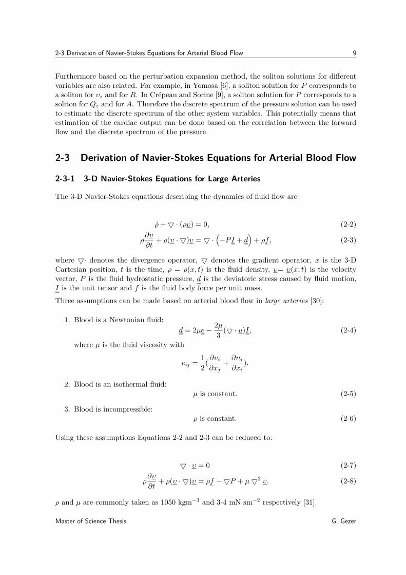
2-3 Derivation of Navier-Stokes Equations for Arterial Blood Flow
2-3-1 3-D Navier-Stokes Equations for Large Arteries
The 3-D Navier-Stokes equations describing the dynamics of fluid flow are
ρ̇+5 · (ρυ) = 0, (2-2)
ρ∂υ
∂t+ ρ(υ · 5)υ = 5 ·
(−PI + d
)+ ρf, (2-3)
where 5· denotes the divergence operator, 5 denotes the gradient operator, x is the 3-DCartesian position, t is the time, ρ = ρ(x, t) is the fluid density, υ= υ(x, t) is the velocityvector, P is the fluid hydrostatic pressure, d is the deviatoric stress caused by fluid motion,I is the unit tensor and f is the fluid body force per unit mass.Three assumptions can be made based on arterial blood flow in large arteries [30]:
1. Blood is a Newtonian fluid:d = 2µe− 2µ
3 (5 · u)I, (2-4)
where µ is the fluid viscosity with
eij = 12( ∂υi∂xj
+ ∂υj∂xi
).
2. Blood is an isothermal fluid:µ is constant. (2-5)
3. Blood is incompressible:ρ is constant. (2-6)
Using these assumptions Equations 2-2 and 2-3 can be reduced to:
5 · υ = 0 (2-7)
ρ∂υ
∂t+ ρ(υ · 5)υ = ρf −5P + µ52 υ. (2-8)
ρ and µ are commonly taken as 1050 kgm−3 and 3-4 mN sm−2 respectively [31].
Master of Science Thesis G. Gezer

10 Biomechanical Design Part
2-3-2 Non-dimensional Form of the Navier-Stokes Equations
The variables in Equations 2-7 and 2-8 are scaled to non-dimensional form using the followingvariable transformations [30]:
x∗ = 1Rd
x, t∗ = tω, v∗ = 1υmean
v, P ∗ = 1ρυ2
meanP, f∗ = Rd
υ2mean
f, (2-9)
where Rd is the vessel radius at diastolic phase, ω is the angular frequency of flow variationand υmean is the mean velocity at the inlet of the artery. Dimensionless Reynolds and Strouhalnumbers describing fluid dynamics, denoted by Re and St respectively, are defined as
Re = ρRdυmeanµ
, St = ωRdυmean
. (2-10)
Using Equations 2-9 and 2-10 Navier-Stokes equations can be described in non-dimensionalform:
5 · υ∗ = 0, (2-11)
St∂υ
∂t
∗+ υ∗ · 5υ∗ − 1
Re52 υ∗ +5P ∗ = f∗. (2-12)
Based on Equations 2-11 and 2-12, for large Reynolds numbers the nonlinear convective term,υ∗ ·5υ∗, dominates the viscous term, 1
Re 52 υ∗. Based on the measurements of flow pulses in
canine arteries [32], this is assumed to be the case so the viscosity term is neglected, leadingto further reduced 3-D Navier-Stokes equations:
∂υ
∂t+ (υ · 5)υ + 1
ρ5 P = f, (2-13)
5 · υ = 0. (2-14)
G. Gezer Master of Science Thesis

2-4 1-D Modeling of Arterial Blood Flow 11
2-4 1-D Modeling of Arterial Blood Flow
Section 2-4 and its subsections are adapted from the literature survey.
2-4-1 Reduction of 3-D Navier-Stokes Equations to 1-D
The solitary wave literature on modeling arterial blood flow is based on 1-D Navier-Stokesequations [6, 29, 27, 8, 9, 11, 14]. This makes the assumptions followed for dimension reductionrelevant for these works. In order to reduce 3-D Navier-Stokes equations (Equations 2-13 and2-14) to 1-D form, the following ideal vessel geometry assumptions are made:
1. The artery is modeled after a cylinder resting in horizontal position. Due to this choicecylindrical coordinates, (z, r, θ), are chosen for representation over Euclidean coordi-nates, (x1, x2, x3). z is the longitudinal coordinate and increases in the direction awayfrom the heart whereas (r, θ) pair refer to the polar coordinates of the cross-section atz. A diagram of the cylindrical coordinate representation of the artery is provided inFigure 2-6.
rzθ
Figure 2-6: Cylindrical coordinates chosen for blood vessel representation.
2. The artery is assumed to be symmetrical around longitudinal axis (axisymmetry), there-fore dependencies on and the dynamics of θ are excluded.
3. The radial flow dynamics are excluded.
4. The derivatives with respect to r are excluded in the dynamics based on the thin cylinderassumption. Based on this assumption:
L� Rd, (2-15)
where L is the vessel length.
5. The terms multiplied with the radial velocity, υr instead of the longitudinal velocity,υz, are neglected based on the assumption
υz � υr. (2-16)
Master of Science Thesis G. Gezer

12 Biomechanical Design Part
Using these assumptions, the 3-D model described by Equations 2-13 and 2-14 can be reducedto 1-D form:
∂υz∂t
+ υz∂υz∂z
+ 1ρ
∂P
∂z= fzρA
, (2-17)
∂A
∂t+ ∂(Aυz)
∂z= 0, (2-18)
where fz = fz(vz) = fA is the axial friction force per length. The volumetric flow in the
longitudinal direction, Qz, is the product of the cross-sectional area and the longitudinalvelocity:
Qz = Aυz, (2-19)
where A = A(z, t) = πR2 is the vessel cross-sectional area and R = R(z, t) is the vessel radius.Equations 2-17 and 2-18 can alternatively be written in terms of Qz:
∂Qz∂t
+ ∂
∂z
(Q2z
A
)+ A
ρ
∂P
∂z= fz
ρ, (2-20)
∂A
∂t+ ∂Qz
∂z= 0. (2-21)
2-4-2 Peripheral Friction Model
The frictional force in the longitudinal direction for an incompressible Newtonian fluid forthe axisymmetric vessels is given as follows [33]:
fz = 2πµR∂ (Fυz)∂r
|r=R , (2-22)
where F = F (r) is the radial velocity profile. Based on Equation 2-22, the friction depends onthe flow value at r = R, which is the reason this type of friction is also referred to as peripheralfriction, associated to the interaction of blood with the vessel wall. In the literature, the termviscous friction is also commonly used as fz scales linearly with µ. In fact, in modelingliterature friction is referred to as viscous effect. In our paper, friction is considered as aseparate effect whereas viscous effects are considered to correspond to viscosity dependentsecond order spatial dynamics in Navier-Stokes equations.
Based on Equation 2-22, F is needed to derive fz. Polynomial radial velocity profile of orderΓ is assumed [34] such that
F = Γ + 2Γ
[1−
(r
R
)Γ]. (2-23)
G. Gezer Master of Science Thesis

2-4 1-D Modeling of Arterial Blood Flow 13
Based on the experimental studies by Hagen [35] and Poiseuille [36] on steady laminar flow ofwater in the cylindrical pipes, F is found to have a parabolic shape (Γ = 2). This assumptionis used throughout in the existing solitary wave literature on arterial blood pressure modeling[6, 29, 27, 8]. However based on Smith et al.’s analysis of blood flow through a geometricmodel of the coronary network in different points of the cardiac cycle [33], F is found to havea higher polynomial order instead (Γ = 9). In this paper, Γ = 9, is assumed based on Smithet al’s findings. By substituting Equation 2-23 into Equation 2-22, the following frictionalforce is obtained:
fz = −2πµ(Γ + 2)υz = −2πµ(Γ + 2)QzA. (2-24)
2-4-3 Linear Elastic Arterial Wall Model
The arterial wall is modeled after a thin, incompressible, homogenous, isotropic membrane[37]. Furthermore the arterial wall is assumed to deform axisymmetrically and the longitudinaldeformations are ignored. The membrane is assumed to participate in only linear elasticdeformation. Under these assumptions the material law is defined as [37]
P = P0 + 4Eh03R2
0(R−R0), (2-25)
where P0 is the reference pressure, E is the Young’s elastic modulus, R0 is the vessel radius atthe reference pressure and h0 is the reference vessel wall thickness at the reference pressure.The reference pressure in our paper will be taken as P0 = 0, when the internal pressure ofthe vessel equals to the external pressure [37].
Master of Science Thesis G. Gezer

14 Biomechanical Design Part
2-5 Derivation of KdV Equations from 1-D Navier-Stokes Equa-tions
In this section, derivation of the KdV type dynamics from 1-D Navier-Stokes equations inYomosa [6] and Créapau and Sorine [9] are discussed. Interested readers can find moreinformation on the scaling of KdV Equation in Appendix A.
2-5-1 Yomosa’s Model
In 1986, Yomosa [6] proposed a soliton theory for a simplified and idealized model-systemthe blood motion in large arteries. Yomosa’s model can derive a relationship between thewidth, the amplitude and the group velocity of the flow and pressure pulses. Instead ofinterpreting the wave as a linear superposition of a backward and a forward component, thewave is interpreted as a nonlinear superposition of only forward components consisting of of2 to 3 solitons. As the peripheral friction is neglected in Yomosa’s work, his model does notaccount for the energy losses which means Yomosa’s model can not describe the pressure asa decreasing function away from the heart. The steepening of the arterial blood pressure isexplained in Yomosa’s work in the context of nonlinear superposition principle of solitons. Inthis subsection, the model and the derivations of [6] will be discussed and referred to by theauthor name, Yomosa.
In Yomosa, the following model assumptions are made:
1. Blood is modeled as an isothermal, incompressible, Newtonian fluid (Section 2-3-1).
2. Viscous term in the blood dynamics is excluded (Section 2-3-2).
3. Friction term in the blood dynamics is excluded (Section 2-4-2).
4. The blood vessel is modeled as an infinitely long, straight cylinder.
5. 1-D dynamics are used over 3-D dynamics (Section 2-4-1).
6. The vessel wall is modeled as a thin, homogenous, elastic membrane. This correspondsto an extension of the static material law described in Equation 2-4-3 to a dynamiclaw with an additional parameter, a, which when set as non zero, makes the staticcomponent of P a nonlinear function of R.
Based on these assumptions in Yomosa, the provided system equations are
∂Qz∂t
+ ∂
∂z
(Q2z
A
)+ 1ρA∂P
∂z= 0, (2-26)
∂A
∂t+ ∂Qz
∂z= 0, (2-27)
P = Eh0R3
0(R−R0) (aR+ (1− a)R0) + ρwH
∂2R
∂t2, (2-28)
G. Gezer Master of Science Thesis

2-5 Derivation of KdV Equations from 1-D Navier-Stokes Equations 15
where Qz = Qz(z, t) is the volumetric flow rate, P = P (z, t) is the pressure, R = R(z, t) isthe vessel radius, A = A(z, t) = πR2 is the vessel cross-sectional area, ρ is the blood density,E is the elastic Young’s modulus, h0 is the reference vessel wall thickness, R0 is the referencevessel radius, a is the nonlinear coefficient of elasticity, ρw is the vessel wall density andH = H(z, t) = h+h′ is the effective inertial thickness where h = h(z, t) is the vessel thicknessthat participates in elastic deformation and h′ is the vessel thickness that does not. Thereference length measurements are taken at P = 0, specifically when the external pressureof the vessel equals to the internal pressure. It should be noted that in Yomosa’s work, thelongitudinal velocity, υz = υz(z, t), is used as a model variable, instead of Qz = Aυz.
Using various asymptotic methods, Yomosa reduces the system equations to three KdV typeequations for each model variable, specifically for υz, P and R. Yomosa’s derivations can besummarized in the following steps.
1. t, z, υz, P and R are scaled to dimensionless variables t∗, z∗, υ∗z , P ∗ and γ∗ respec-tively using physical model parameters. The dimensionless variables are used to convertEquations 2-26, 2-27 and 2-28 to non-dimensional form.
2. A linear dispersion relation is acquired for the non-dimensional nonlinear problem. Todo so, first nonlinear terms in the dynamics are neglected to obtain linearized set ofequations. Then harmonic solutions are assumed for the dimensionless variables so that
υ∗z , P∗, γ∗ ∝ ei(kz∗−ωt∗), (2-29)
and the non-vanishing solutions of the form w(k) = gf(k) are obtained when the deter-minant of the system equals to zero. g is the group velocity and f(k) denotes a functionof k, which is the wavenumber.
3. D’Alembert’s solution for a right traveling wave is considered such that
z∗ − gt∗,
is used over the space variable z∗.
4. Using long wave estimation (Appendix D), the scaling variable ε is introduced to scalethe time variable and the new space variable:
ξ = ε12 (z∗ − gt∗), τ = ε
32 t∗. (2-30)
5. The dimensionless variables are expressed as power series of ε:
υ∗z =∞∑n=1
εnυn(ξ, τ), (2-31)
P ∗ =∞∑n=1
εnpn(ξ, τ), (2-32)
γ∗ =∞∑n=1
εnγn(ξ, τ), (2-33)
and this power expansion is substituted into the non-dimensional equation. The termsscaled with ε3 and higher powers are neglected under small ε assumption.
Master of Science Thesis G. Gezer
16 Biomechanical Design Part
6. Perturbation expansion is done by grouping and solving the terms scaled with samepowers of ε. In particular, this leads to three set of equations that scale with ε0, ε1 andε2 respectively.
7. Using realistic boundary conditions and solving for the terms scaled with ε1, the expan-sion variables υ1, p1 and γ1 are related to each other.
8. Using these relationships, the terms proportional to ε2 are solved to relate υ2, p2 andγ2 to υ1, p1 and γ1. Then, the terms proportional to ε2 are expressed in terms of υ1, p1and γ1 which leads to KdV type equations.
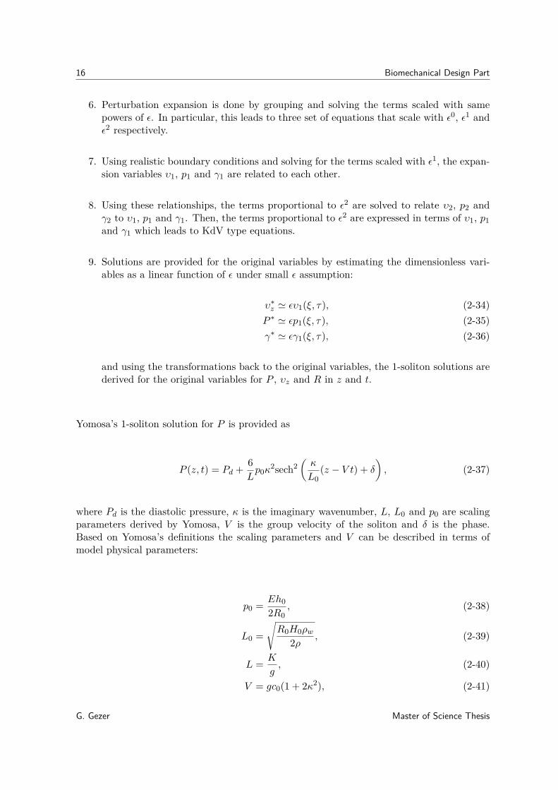
9. Solutions are provided for the original variables by estimating the dimensionless vari-ables as a linear function of ε under small ε assumption:
υ∗z ' ευ1(ξ, τ), (2-34)P ∗ ' εp1(ξ, τ), (2-35)γ∗ ' εγ1(ξ, τ), (2-36)
and using the transformations back to the original variables, the 1-soliton solutions arederived for the original variables for P , υz and R in z and t.
Yomosa’s 1-soliton solution for P is provided as
P (z, t) = Pd + 6Lp0κ
2sech2(κ
L0(z − V t) + δ
), (2-37)
where Pd is the diastolic pressure, κ is the imaginary wavenumber, L, L0 and p0 are scalingparameters derived by Yomosa, V is the group velocity of the soliton and δ is the phase.Based on Yomosa’s definitions the scaling parameters and V can be described in terms ofmodel physical parameters:
p0 = Eh02R0
, (2-38)
L0 =√R0H0ρw
2ρ , (2-39)
L = K
g, (2-40)
V = gc0(1 + 2κ2), (2-41)
G. Gezer Master of Science Thesis

2-5 Derivation of KdV Equations from 1-D Navier-Stokes Equations 17
with
K = (1 + γ0) (1 + 2a+ 3(2a− 1)γ0)4 (1 + (2a− 1)γ0)
32
,
g =√
1 + (2a− 1)γ01 + γ0
,
c0 =√Eh02ρR0
,
Pdp0
= 2γ0(1 + aγ0)(1 + γ0)2 .
KdV equations for the original variables, P , υz and R are not provided explicitly in Yomosa’swork. We will derive the KdV equation for P expressed in z and t following Yomosa’snormalization steps. In Yomosa, the following KdV equation is provided for p1:
∂p1∂τ
+ Lp1∂p1∂ξ
+ 12∂3p1∂ξ3 = 0. (2-42)
Following the normalization steps for time and space variables in Yomosa’s work, ξ and τ canbe described as a function of z and t:
ξ = ε12
L0(z − gc0t) , τ = ε
32 gc0L0
t (2-43)
which is used to express Equation 2-42 in terms of z and t:
∂p1∂t
+ gc0(1 + εLp1)∂p1∂z
+ gc0L20
2∂3p1∂z3 = 0. (2-44)
Following Yomosa’s normalization steps, p1 can be described as an affine function of P :
p1 '1εP ∗ = 1
εp0(P − Pd), (2-45)
which can be used to derive KdV-type dynamics for P :
∂P
∂t+ gc0L
p0
(p0L− Pd + P
)∂P
∂z+ gc0L
20
2∂3P
∂z3 = 0. (2-46)
The solution to this equation can be determined uniquely if the initial data decays sufficientlyrapidly. The initial data is considered to be fixed in time:
Pini = P (z, t0). (2-47)
In practical applications we are interested in solving for initial data fixed in z instead. This isdue to the fact that clinical measurements of arterial blood pressure is done at fixed positions
Master of Science Thesis G. Gezer

18 Biomechanical Design Part
making space evolution of interest over time evolution. Equation 2-46 can be convertedtimelike KdV equation referring to the work of Osborne and Petti [38]. First P is normalizedsuch that the vertical offset is removed.
P̂ = P − Pd (2-48)
which leads to the spacelike KdV Equation
∂P̂
∂t+ gc0
∂P̂
∂z+ gc0L
p0P̂∂P̂
∂z+ gc0L
20
2∂3P̂
∂z3 = 0. (2-49)
Then, based on [38], the spacelike KdV Equation is converted to an estimated timelike form:
∂P̂
∂z+ 1gc0
∂P̂
∂t− L
gc0p0P̂∂P̂
∂t− L2
02
∂3P̂
∂t3= 0, (2-50)
such that the associated initial data is fixed in position instead
P̂ini = P (z0, t)− Pd. (2-51)
2-5-2 Crépeau and Sorine’s Model
In 2005, Crépeau and Sorine[7] proposed a reducel model describing the input-output behaviorof an arterial compartment. Based on this model, the arterial blood pressure waveform isinterpreted as finite number of solitons moving in forward direction and the contribution ofthe frictional effects is estimated by a Windkessel. In 2007, Créapau and Sorine revised theirmodel for a different conference submission [9] and Laleg contributed to Crépeau and Sorine’swork by proposing identification method for the soliton components [11]. In particular, in thissubsection, the model and the derivations of [9] will be discussed and referred to by authorname, Crépeau and Sorine.
In Crépeau and Sorine following model assumptions are made:
1. Blood is modeled as an isothermal, incompressible, Newtonian fluid (Section 2-3-1).
2. Viscous term in the blood dynamics is excluded (Section 2-3-2).
3. Frictional term in the blood dynamics is included but the coefficient of the term is notderived based on model physical parameters but rather taken as an arbitrary constant.
4. The blood vessel is modeled as an infinitely long, straight cylinder.
5. 1-D dynamics are used over 3-D dynamics (Section 2-4-1).
6. The vessel wall is modeled as a thin, homogenous, elastic membrane. Pressure is con-sidered to be a linear dynamical function of the vessel cross-sectional area, which makesit a nonlinear function of vessel radius.
G. Gezer Master of Science Thesis

2-5 Derivation of KdV Equations from 1-D Navier-Stokes Equations 19
Based on the aforementioned assumptions Crépeau and Sorine’s system equations are givenas
∂Qz∂t
+ ∂
∂z
(Q2z
A
)+ 1ρA∂P
∂z+ b
QzA
= 0, (2-52)
∂A
∂t+ ∂Qz
∂z= 0, (2-53)
P = Eh02R3
0(R−R0) (R+R0) + 2ρwh0
R0
[R∂2R
∂t2+(∂R
∂t
)2], (2-54)
where Qz = Qz(z, t) is the volumetric flow rate, P = P (z, t) is the pressure, R = R(z, t) isthe vessel radius, A = A(z, t) = πR2 is the vessel cross-sectional area, ρ is the blood density,b is the coefficient of the frictional term, E is the elastic Young’s modulus, h0 is the referencevessel wall thickness, R0 is the reference vessel radius and ρw is the vessel wall density. Thereference length measurements are taken at P = 0.Using various derivations, Crépeau and Sorine reduces this set of equations to three KdVequations for Qz, P and A in a boundary layer. Crépeau and Sorine’s derivations can besummarized as follows:
1. z, t, Qz, P and A are scaled to dimensionless variables z∗, t∗, Q∗z, P ∗ and A∗ usingphysical model parameters. The dimensionless variables are used to convert Equations2-52, 2-53 and 2-54 to non-dimensional form.
2. D’Alembert’s solution for a right traveling wave is considered such that
t∗ − z∗,
is used over the time variable t∗.
3. Using long wave estimation (Appendix D), the scaling variable ε is introduced to scalethe space variable and the new time variable:
τ = t∗ − zε2
, ξ = z∗
ε. (2-55)
An explicit definition for ε is also provided:
ε =(R0L0
) 25, (2-56)
where L0 is the typical wave length of the waves propagating in the tube.
4. The dimensionless variables are expressed as power series of ε:
Q∗z =∞∑n=1
εnQn(ξ, τ), (2-57)
P ∗ =∞∑n=1
εnpn(ξ, τ), (2-58)
A∗ =∞∑n=1
εnAn(ξ, τ), (2-59)
Master of Science Thesis G. Gezer

20 Biomechanical Design Part
and this power expansion is substituted into the non-dimensional equation. The termsscaled with ε3 and higher powers are neglected under small ε assumption.
5. Perturbation expansion is done by grouping and solving the terms scaled with samepowers of ε. In particular, this leads to three set of equations that scale with ε0, ε1 andε2 respectively.
6. Using the relationships of the variables and assuming fast times in a boundary layer,the equations obtained from the perturbation expansion are solved for Q1, p1 and A1,leading to KdV type equations in timelike form.
7. The dimensionless variables are estimated as an linear function of ε under small ε as-sumption:
Q∗z ' εQ1(ξ, τ), (2-60)P ∗ ' εp1(ξ, τ), (2-61)A∗ ' εA1(ξ, τ). (2-62)
and using the transformations back to the original variables from dimensionless vari-ables, the KdV equation for Qz is obtained.
8. The frictional effects are neglected based on fast times in a boundary layer assumption,but assuming large time or space a parabolic equation for Qz is obtained instead:
∂Qz∂t− A0h0E
2ρbR0
∂2Qz∂z2 = 0, (2-63)
whose low frequency approximation is used to estimate a 2 or 3 element Windkessel.
In Crépeau and Sorine’s work, the KdV equation representing the fast blood flow is providedin initial variables:
∂Qz∂z
+ d0∂Qz∂t
+ d1∂Qz∂t
Qz + d2∂3Qz∂t3
= 0, (2-64)
with
d0 = 1c0, d1 = − 3
2A0c20, d2 = −ρwh0R0
2ρc30, (2-65)
where c0 is Moens-Korteweg velocity of a wave propagating in an elastic tube and defined as
c0 =√Eh02ρR0
. (2-66)
The 1-soliton solutions for Qz and P are not explicitly provided in Crépeau and Sorine. Firstwe will derive the denormalized 1-soliton solution for Qz following the normalization steps inCrépeau and Sorine. Consider a standard KdV equation of the form
G. Gezer Master of Science Thesis

2-5 Derivation of KdV Equations from 1-D Navier-Stokes Equations 21
∂U
∂Z+ 6∂U
∂TU + ∂3T
∂Z3 = 0, (2-67)
whose 1-soliton solution is given as
U(Z, T ) = 12κ
2sech2(κ
2 (T − κ2Z) + δ
). (2-68)
Using the following transformations [11]
T = t− d0z, Z = d2z, U = d16d2
Qz (2-69)
the denormalized 1-soliton solution for Equation 2-64 can be derived as
Qz(z, t) = 3d2d1
κ2sech2(κ
2 (t− d0z − d2κ2z) + δ
), (2-70)
where κ is the imaginary wavenumber and δ is the phase. The 1-soliton solution for P canbe calculated using the following equations provided in Crépeau and Sorine:
Qz = A0c0Q1, P = ρc20P1 + Pd, P1 = Q1, (2-71)
leading to the 1-soliton solution for P :
P (z, t) = Pd + 3ρc0d2A0d1
κ2sech2(κ
2 (t− d0z − d2κ2z) + δ
). (2-72)
The linear transformations in Equation 2-71 can used along with Equation 2-64 to deriveKdV-type dynamics for P :
∂P
∂z+(d0 −
A0ρc0
Pd
)∂P
∂t+ d1
(A0ρc0
)P∂P
∂t+ d2
∂3P
∂t3= 0. (2-73)
P is normalized to remove the vertical offset so that
P̂ = P − Pd, (2-74)
which leads to the KdV Equation
∂P̂
∂z+ d0
∂P̂
∂t+ d1
(A0ρc0
)P̂∂P̂
∂t+ d2
∂3P̂
∂t3= 0. (2-75)
The associated initial data for the problem then becomes
P̂ini = P (z0, t)− Pd. (2-76)
Master of Science Thesis G. Gezer
22 Biomechanical Design Part
2-6 Model Matching
The simulation model and the KdV models have different model assumptions, so these differ-ences have to be addressed for the verification of KdV type dynamics and soliton solutions.We propose imposing consistency between models by adjusting the physical model parametersof KdV models.
2-6-1 Fundamental Challenges of Testing Korteweg-de Vries Dynamics
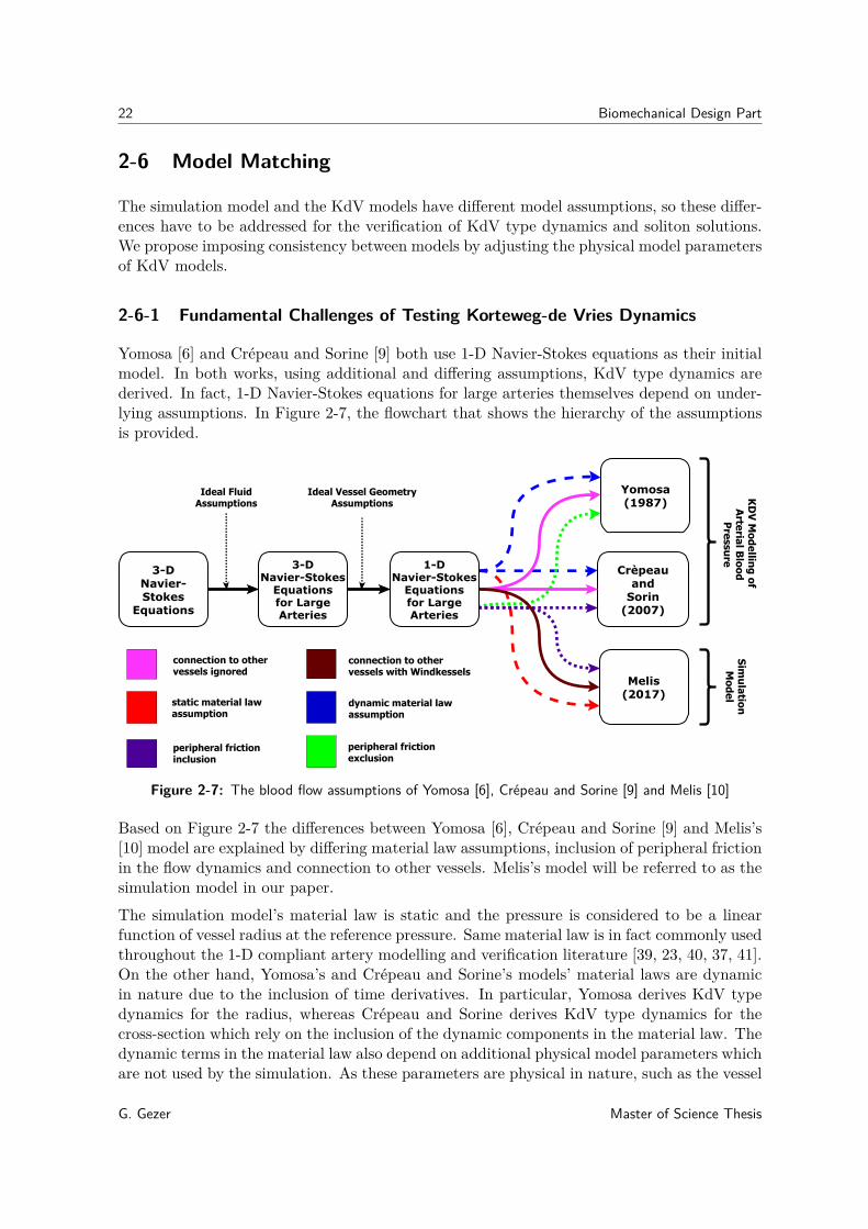
Yomosa [6] and Crépeau and Sorine [9] both use 1-D Navier-Stokes equations as their initialmodel. In both works, using additional and differing assumptions, KdV type dynamics arederived. In fact, 1-D Navier-Stokes equations for large arteries themselves depend on under-lying assumptions. In Figure 2-7, the flowchart that shows the hierarchy of the assumptionsis provided.
3D NavierStokes
Equations
3D NavierStokesEquations for LargeArteries
Yomosa (1987)
Crèpeau and Sorin (2007)
Melis (2017)
Ideal FluidAssumptions
Ideal Vessel GeometryAssumptions
KDV Modelling of
Arterial B
loodPressure
Simulation Model
1D NavierStokes Equations for LargeArteries
peripheral frictionexclusion
peripheral frictioninclusion
dynamic material lawassumption
static material lawassumption
connection to othervessels with Windkessels
connection to othervessels ignored
Figure 2-7: The blood flow assumptions of Yomosa [6], Crépeau and Sorine [9] and Melis [10]
Based on Figure 2-7 the differences between Yomosa [6], Crépeau and Sorine [9] and Melis’s[10] model are explained by differing material law assumptions, inclusion of peripheral frictionin the flow dynamics and connection to other vessels. Melis’s model will be referred to as thesimulation model in our paper.
The simulation model’s material law is static and the pressure is considered to be a linearfunction of vessel radius at the reference pressure. Same material law is in fact commonly usedthroughout the 1-D compliant artery modelling and verification literature [39, 23, 40, 37, 41].On the other hand, Yomosa’s and Crépeau and Sorine’s models’ material laws are dynamicin nature due to the inclusion of time derivatives. In particular, Yomosa derives KdV typedynamics for the radius, whereas Crépeau and Sorine derives KdV type dynamics for thecross-section which rely on the inclusion of the dynamic components in the material law. Thedynamic terms in the material law also depend on additional physical model parameters whichare not used by the simulation. As these parameters are physical in nature, such as the vessel
G. Gezer Master of Science Thesis

2-6 Model Matching 23
wall density, it is possible to refer to literature to come up with valid values. Unfortunatelythis is not the case for all additional parameters assumed by Yomosa - although Yomosaderives a soliton solution based on physical parameters, in his benchmark tests two of theadditional parameters, specifically nonlinear coefficient of elasticity, a, and thickness of thearterial wall that does not participate in elastic deformation, h′, are treated as fit variablesbased on additional assumptions on the solution. To the extent of our knowledge, theseparticular parameters do not have reference values or even ranges in the existing literature.Testing Yomosa’s solution for a range of these values is also problematic in nature as thesimulation model’s material law lacks a dynamic component, making over-fitting a relevantproblem for testing Yomosa’s model.
Another difference between the models arises from the inclusion or exclusion of terms in the1-D Navier-Stokes momentum equation. The simulation model and Crépeau and Sorine’smodel both include frictional term in the dynamics, whereas Yomosa’s model does not. Asthe inclusion of friction correspond to energy losses over wave propagation, this violates theenergy conservation principles of the soliton solutions over large space or time propagation.This in fact explains why Yomosa’s model can not explain the decrease of pressure as functionof increasing longitudinal distance. Crépeau and Sorine tackles this issue, by restricting thedefinition of proposed soliton solutions to boundary layers which removes the effects of thefriction due to fast times assumption. For large space or time propagation, the effects offriction is estimated with a 2 or 3-element Windkessel (described in Figures 2-2 and 2-3respectively). In the simulation model, peripheral friction is included in the dynamics and isderived based on Equation 2-24. Setting the viscosity parameter, µ, to zero in the simulationinitialization file can eliminate the effects of peripheral friction. The existing literature on1-D modelling of compliant arteries accounts for the effects of friction in the flow dynamics[39, 40, 37, 41, 10] so in our tests we will include the effects of friction in the dynamics aswell.
Last but not least, assumption on connection to other vessels plays an important part inthe arterial blood pressure dynamics. In Yomosa’s model, the artery is assumed to be in-finitely long, which means physical reflections caused by the interconnections of arteries areneglected. In Crépeau and Sorine, the assumptions on reflections are not explicitly addressed;specifically Crépeau and Sorine restrict their derivations to describe the dynamics of the ar-terial compartment of a single artery. In the simulation, connections to other vessels canbe accounted for by imposing outlet boundary conditions using 2 or 3-element Windkessels.Alternatively, the reflection type outlet can be chosen in the simulation model and by settingthe reflection parameter, Rt, to zero, the connections to other vessels can be neglected tomatch the assumptions of Yomosa’s and Crépeau and Sorine’s model. In our tests, the effectsof connections to the other vessels will be considered as clinical pressure measurements aresubject to the interconnection effects. Windkessels can represent the effects of interconnectionin a simple manner by assigning a hydraulic impedance at the outlet which can be effectiveto explain the steepening phenomena (described in Section 2-2-1). In contrast, Crépeau andSorine describe the Windkessel dynamics based derivations of 1-D Navier-Stokes equationsand the assumed material law. The values of the Windkessel elements are not explicitly givenin Crépeau and Sorine but treated as fit variables in the benchmark tests with real patientpressure measurements. As the experimental data is subject to network effects, the fittedWindkessel elements might be representing effects beyond friction in the dynamics. In ourpaper, the 3-element Windkessels will be used to model reflections caused by network effects,
Master of Science Thesis G. Gezer

24 Biomechanical Design Part
consistent with its definition in the simulation model.
The ideal fluid and vessel geometry assumptions used for the derivation of 1-D Navier-Stokesequations (Figure 2-7) also impose fundamental limitations on physiological implications ofour testing. Xiao et al. [37] address the ideal vessel geometry assumptions by comparing 1-Dand 3-D compliant artery models using consistent physical parameters and boundary condi-tions. Based on the results of Xiao et al., both formulations are in good agreement. The idealfluid assumptions will not be fully addressed in the scope of our work. The incompressiblefluid behavior is an estimation of a conceptually unphysical phenomenon; as a truly incom-pressible fluid would require the sound waves to travel at an instant throughout the fluid,violating the concept of causality. In the smaller vessels non-Newtonian effects may also playa role [30] and these effects may be potentially relevant for larger vessels. In a nutshell, 1-DNavier-Stokes representation may not be able to represent the real physiological phenomenaaccurately. Addressing such a problem would require benchmarking 1-D Navier-Stokes equa-tions against accurate in vivo measurements, which might be challenging in its own way aspressure and flow relationship of human subjects differ in an individual level and betweendifferent groups. This the main reason, we want to test KdV type dynamics and associatedsoliton solutions against 1-D Navier-Stokes equations, as this approach removes dependencieson ideal fluid and vessel geometry assumptions in the reference and tested behavior. To ver-ify KdV type equations for arterial blood pressure, the ideal fluid and ideal vessel geometryassumptions have to be properly addressed to verify results at the physiological level.
2-6-2 Blood Flow Simulation Software and Model
openBF is an open-source 1D blood flow solver based on MUSCL finite-volume numericalscheme, written in Julia and released under Apache 2.0 free software license. The docu-mentation of openBF, the benchmark tests that compares the results with existing modelingliterature is provided in the PhD dissertation of Melis [10].
The blood flow model of openBF is based on the following model assumptions:
1. Blood is modeled after an incompressible and isothermal Newtonian fluid. This assump-tion is used for the derivation of 3-D Navier Stokes equations (Section 2-3-1).
2. Viscosity term in the blood dynamics is excluded (Section 2-3-2).
3. The vessel is modeled after a thin axisymmetric cylinder which is used to reduce the3-D dynamics to 1-D (Section 2-4-1).
4. The friction model is derived under polynomial radial velocity profile assumption (Sec-tion 2-4-2).
5. The vessels are straight and have linearly elastic compliant walls (Section 2-4-3).
G. Gezer Master of Science Thesis

2-6 Model Matching 25
The simulation model is given as follows:
∂Qz∂t
+ ∂
∂z
(Q2z
A
)+ A
ρ
∂P
∂z+ 2µ
ρ(Γ + 2)Q
A= 0, (2-77)
∂A
∂t+ ∂Qz
∂z= 0, (2-78)
P = 4Eh03R2
0(R−R0), (2-79)
where t is time, z is the longitudinal position, R = R(z, t) is the vessel radius, A = A(z, t) =πR2 is the vessel cross-sectional area, Qz is the longitudinal volumetric flow rate, P is theblood pressure, ρ is the blood density, µ is the blood viscosity, Γ is the polynomial fit orderassumed for the radial velocity profile, E is the vessel wall elastic Young’s modulus, h0 is thereference vessel wall thickness and R0 is the reference vessel radius. In this paper, Equations 2-77, 2-78 and 2-79 will be referred to as the simulation’s equation of motion, mass conservationprinciple and material law respectively. As an important remark, the solver has the hybridmodel structure described in Figure 2-5. The system boundary conditions are applied to theinlet and the outlet of the vessel. The inlet boundary conditions describe the time evolutionfixed at the initial location and can be in terms of P or Q based on user choice:
Pin(t) = P (z0, t), (2-80)Qin(t) = Q(z0, t), (2-81)
where Pin and Qin are the considered pressure and volumetric flow rate boundary conditions atthe inlet respectively. The solver assumes the time data to be normalized on the cardiac cycleperiod, Tc. Therefore the boundary conditions are expected to represent the values within acardiac cycle, with time data scaled to the domain [0, 1]. The inlet boundary conditions aretreated as periodic.The user is expected to enter model physical parameters in a yml file. In this file also solverparameters have to be specified. The solver runs for multiple cardiac cycles until the differencebetween the output signals in the current and previous cycle are found be within the userdefined error tolerance. The maximum number of cardiac cycles and the number of timestepsincluded in the outputs can be specified as well.Outlet boundary conditions should be chosen based on the assumptions to other vessels. Ifthe vessel is not connected to another vessel the reflection type outlet should be chosen andthe reflection coefficient, Rt, has to be provided. If the vessel is connected to another vessel,2 or 3-element Windkessel type outlets should be chosen and then the values of Windkesselelements have to be provided.If a network of arteries are simulated, the junctions of the components have to be specified.The inlet boundary conditions have to be assigned only to the input components of thenetwork. Outlet types and parameters, have to be assigned only to the output components.
2-6-3 Yomosa’s and Simulation Model Matching
Yomosa’s material law (Equation 2-28) is different compared to the simulation’s material law(Equation 2-79). In particular, in Yomosa’s model [6]:
Master of Science Thesis G. Gezer
26 Biomechanical Design Part
1. The acceleration of the vessel radius is included in the material law resulting with adynamic material law instead of a static one.
2. P is a quadratic function of R, if the nonlinear coefficient of elasticity a is non-zero andthe acceleration term is ignored.
3. P is scaled with 1 instead of 43 , if the acceleration term is ignored.
These steps are proposed for imposing consistency between Yomosa’s model and the simula-tion model.
1. The acceleration term in Yomosa’s material law can not be taken into considerationby the simulation model which assumes a static material law. However neglecting thismismatch between the models is a reasonable option as the scaling of the accelerationterm is very small; in standard units ρw scales with 103, H scales with 10−3 and withina cardiac cycle P variation scales with 104.
2. The acceleration term in Yomosa’s material law is scaled by ρw and H which are notconsidered parameters in the simulation model but are included in Yomosa’s solitonsolution. Furthermore as the inclusion of dynamics in the material law is fundamentalto the derivation of Yomosa’s solution, the acceleration term can not be cancelled bysetting ρw or H to zero. ρw will be considered to match ρ used in the simulation modelas the vessel wall density and the blood density are almost equal in the physiologicalsystems leading to the relation:
ρw = ρ. (2-82)
Yomosa defines H as the sum of h, which is the vessel thickness that participates in theelastic deformation and h′, the vessel thickness that does not [6]. Although the value ofH at the reference pressure, H0, is included as a parameter in Yomosa’s solution, theparameter is treated as a fit parameter in Yomosa’s benchmark tests. In Yomosa, H0is estimated based on additional assumptions on the solution which makes Yomosa’sestimates of H0 questionable for generic applications. Due to this, the thickness of thewall that does not participate in elastic deformation will be ignored in the solution,leading to the equation:
H0 = h0. (2-83)
This also imposes consistency between Yomosa’s and simulation model as in the simu-lation model entire vessel thickness is considered to participate in linear deformation.
3. If the acceleration term is ignored, Yomosa’s material law can be reduced to a linearstatic function as the simulation model when a is set to zero. Since the simulation modelhas a linear static law, a will be set as zero to match model behavior:
a = 0. (2-84)
G. Gezer Master of Science Thesis

2-6 Model Matching 27
4. E is scaled by a factor of 43 to compensate for the coefficient difference between the
models:
EY = 43E. (2-85)
Yomosa introduces E only for the material law and does not use it in intermediate stepsbeyond this context so the coefficient can be absorbed without changing the nature ofthe solution.
The matched Yomosa’s 1-soliton solution for P is given as
P (z, t) = Pd + 6Lp0κ
2sech2(κ
L0(z − V t)− δ
), (2-86)
where κ is the imaginary wavenumber, L, L0 and p0 are scaling parameters derived by Yomosa,V is the group velocity of the pressure soliton and δ is the phase. To address material lawinconsistencies, it is assumed that a = 0, ρw = ρ, H0 = h0 and EY = 4
3E. The matched scalingparameters and the matched V can be described in terms of model physical parameters:
p0 = EY h02R0
, (2-87)
L = K
g, (2-88)
L0 =
√R0h0
2 , (2-89)
V = gc0(1 + 2κ2
), (2-90)
with
K = (1 + γ0)(1− 3γ0)4(1− γ0)
32
,
g =√
1− γ01 + γ0
,
c0 =√EY h02ρR0
,
Pdp0
= 2γ0(1 + γ0)2 .
The matched parameters can be plugged into the timelike KdV equation (Equation 2-50),leading to the matched KdV equation
∂P̂
∂z+ 1gc0
∂P̂
∂t− L
gc0p0P̂∂P̂
∂t− L2
02
∂3P̂
∂t3= 0. (2-91)
Master of Science Thesis G. Gezer

28 Biomechanical Design Part
with
P̂ = P − Pd. (2-92)
The associated initial data for the match KdV equation is
P̂ini = P (z0, t)− Pd. (2-93)
2-6-4 Crépeau and Sorine’s and Simulation Model Matching
Crépeau and Sorine’s material law (Equation 2-54) is different compared to the simulation’smaterial law (Equation 2-79). In particular, in Crépeau and Sorine’s model:
1. The acceleration of the vessel cross-section is included in the material law resulting witha dynamic material law instead of a static one.
2. P is a linear function of A which makes it a quadratic function of R, if the accelerationterm is ignored.
3. P is scaled with 1 instead of 43 , if the acceleration term is ignored.
These steps are proposed for imposing consistency between Crépeau and Sorine’s model andthe simulation model.
1. The acceleration term in Crépeau and Sorine’s material law can not be taken intoconsideration by the simulation model which assumes a static material law. Howeverneglecting this mismatch between the models is a reasonable option as the scaling ofthe acceleration term is very small; in standard units ρw scales with 103, h0 scales with10−3 and within a cardiac cycle P variation scales with 104.
2. The acceleration term in Crépeau and Sorine’s material law is scaled by ρw which is nota considered parameter in the simulation model but is included in Crépeau and Sorine’smodel and solution. Furthermore as the inclusion of dynamics in the material law isfundamental to derivation of the Crépeau and Sorine’s solution, the acceleration termcan not be cancelled by setting ρw to zero. ρw will be considered to match ρ used inthe simulation model as the vessel wall density and the blood density are almost equalin the physiological systems leading to the relation:
ρw = ρ. (2-94)
3. If the acceleration term is ignored, Crépeau and Sorine’s material is a linear function ofA which makes it a quadratic function of R as a = πR2. To address this issue, we aredefining the following optimization problem
minEC
∫ 1.04Rd
Rd
(4E(R−R0)
3 − EC(R2 −R20)
2R0
)2
dR, (2-95)
G. Gezer Master of Science Thesis

2-6 Model Matching 29
which returns Young modulus EC that will be used in the matched model instead ofE. The optimization problem minimizes the 2-norm of the difference between the staticcontribution of the material laws between the range [Rd, 1.04Rd]. Rd is the radius atthe diastolic pressure and can be calculated using Equation 2-79:
Rd = 3R20
4Eh0Pd +R0. (2-96)
The upper range in the integral, 1.04Rd is determined based on Chen et al. [42] whichstates that the radius stretch rate is less than 4% in the real arteries. As EC dependson physical model parameters in this formulation, the value of it will be provided in thetests. It should be noted that the optimization problem has an analytical result but dueto its complex form the exact solution is not provided. Crépeau and Sorineintroduce Eonly for the material law and does not use it in intermediate steps beyond this contextso the coefficient can be absorbed without changing the nature of the solution.
The matched Crépeau and Sorine’s 1-soliton solution for P is given as
P (z, t) = Pd + 3ρc0d2A0d1
κ2sech2(κ
2 (t− d0z − d2κ2z) + δ
). (2-97)
where κ is the imaginary wavenumber and δ is the phase with
A0 = πR20, c0 =
√ECh02ρR0
, d0 = 1c0, d1 = − 3
2A0c20, d2 = −h0R0
2c30. (2-98)
The matched parameters can be plugged into the timelike KdV equation (Equation 2-75),leading to the matched KdV equation
∂P̂
∂z+ d0
∂P̂
∂t+ d1
(A0ρc0
)P̂∂P̂
∂t+ d2
∂3P̂
∂t3= 0 (2-99)
with
P̂ = P − Pd. (2-100)
The associated initial data for the matched KdV equation is
P̂ini = P (z0, t)− Pd. (2-101)
Master of Science Thesis G. Gezer

30 Biomechanical Design Part
G. Gezer Master of Science Thesis

Chapter 3
Systems and Control Part
3-1 Case Studies and Physical Model Parameters
We are considering the simplified arterial network and case studies described in Figure 3-1.
CASE Ishort artery
CASE IIlong artery
CASE IIIbranching artery
ascending aorta aorta from ascending part to the thoracic part
abdominal aorta
iliac bifurcation
Figure 3-1: The simple artery network and case studies used for simulations.
In all cases, curvature and tapering of the vessels are neglected. The branching of aorta exceptCase III is also neglected. The simplified artery network output is considered to represent thearterial network from aortic root to the end of iliac bifurcation. The output of the previous
Master of Science Thesis G. Gezer

32 Systems and Control Part
case is considered to be the input of the next case, however in some tests the cases will betreated independently.
For all simulations, the number of time steps is set to 600 and the error tolerance is set to0.1%. The rest of the solver parameters are taken as default.
In the simulations, the connections to other arteries will be addressed using a 3-elementWindkessel and the frictional effects will be also included. As a reminder, the matched KdVmodels are derived based on the exclusion of both connection to other vessels and peripheralfriction. If the tested and the reference behavior is found to be significantly different, first onlythe connection to other vessels, then both the connection to other vessels and the peripheralfriction will be excluded to test whether the mismatch is explained by any of these factors.This way we can test the modeling capabilities of the matched KdV models beyond theirderivation assumptions and also understand whether the derivation of KdV type dynamicsfrom 1-D Navier-Stokes equations under derivation assumptions changes the original behavior.
3-1-1 Case I: Short Artery
R0
E,h0
Pin
l
R2 C
R1Pout
Figure 3-2: Technical drawing of the ascending aorta.
The short artery is modeled after the human ascending aorta. The technical diagram of theascending aorta is provided in Figure 3-2.
The physical model parameters are taken from Melis [10] except the value of Young modulus,E, which is taken from Westerhof et al. [23] and are provided in Table 3-1.
G. Gezer Master of Science Thesis

3-1 Case Studies and Physical Model Parameters 33
Table 3-1: The physical model parameters of the human ascending aorta [10, 23].
Parameter Value
Length, l 4.00 cmRadius at reference pressure, R0 1.47 cm
Wall thickness at reference pressure, h0 1.65 mmYoung’s modulus, E 400 kPa
Windkessel resistance 1, R1 1.31×10⁷ Pa s m−3
Windkessel resistance 2, R2 2.22×10⁷ Pa s m−3
Windkessel compliance C, C 1.61×10⁻⁸ Pa−1 m3
3-1-2 Case II: Long Artery
R0
E,h0
Pin
l
R2 C
R1Pout
Figure 3-3: Technical drawing of the aorta from ascending part to the thoracic part.
The long artery is modeled after the human aorta from ascending part to the thoracic part.The technical diagram of the ascending aorta is provided in Figure 3-3.
The physical model parameters are taken from Melis [10] and are provided in Table 3-2.
Master of Science Thesis G. Gezer

34 Systems and Control Part
Table 3-2: The physical model parameters of the human aorta, from ascending part to thethoracic part [10].
Parameter Value
Length, l 24.1 cmRadius at reference pressure, R0 9.87 mm
Wall thickness at reference pressure, h0 0.82 mmYoung’s modulus, E 400 kPa
Windkessel resistance 1, R1 1.17×10⁷ Pa s m−3
Windkessel resistance 2, R2 1.12×10⁸ Pa s m−3
Windkessel compliance C, C 1.02×10⁻⁸ Pa−1 m3
3-1-3 Case III: Branching Artery
R2 C
R1
R0
E,h0
Pin
l
l
l
R0
R0
E,h0
R2 C
R1
ABDOMINAL AORTA ILIAC BIFURCATION
Pout,1
Pout,2
Figure 3-4: Technical Drawing of the abdominal aorta and the iliac bifurcation.
The network comprising of the human abdominal aorta and the human iliac bifurcation isconsidered for the third case study. The technical diagram of the network is provided inFigure 3-4. The input to the abdominal aorta is considered as the input to the network. Thedistal end of the abdominal aorta is considered to be connected to the proximal ends of iliacbifurcation which consists of two identical arteries. In the tests, the interconnection point of
G. Gezer Master of Science Thesis

3-1 Case Studies and Physical Model Parameters 35
the arteries is taken as the the first reference output and the output of one of the identicaliliac arteries is taken as the second reference output.
The physical model parameters are taken from Melis [10]. The physical parameters of theabdominal aorta and iliac bifurcation components are provided in Tables 3-3 and 3-4 respec-tively.
Table 3-3: The physical model parameters of the abdominal aorta component
Parameter Value
Length, l 8.60 cmRadius at reference pressure, R0 7.58 mm
Wall thickness at reference pressure, h0 0.900 mmYoung’s modulus, E 500 kPa
Table 3-4: The physical model parameters of the iliac bifurcation components
Parameter Value
Length, l 8.50 cmRadius at reference pressure, R0 5.49 mm
Wall thickness at the reference pressure, h0 0.680 mmYoung’s modulus, E 700 kPa
Windkessel resistance 1, R1 6.81×10⁷ Pa s m−3
Windkessel resistance 2, R2 3.10×10⁹ Pa s m−3
Windkessel compliance C, C 3.67×10⁻¹⁰ Pa−1 m3
Master of Science Thesis G. Gezer

36 Systems and Control Part
3-2 Verification of the Matched KdV Models
Pin Matched KDV Model I
Matched KDV ModelII
Simulation PM
PY
PCS
reference output
test outputs
realistic input
Figure 3-5: KdV verification test flowchart followed in each case study.
The flowchart of the verification test of the matched KdV models are provided in Figure 3-5.For the verification of the matched KdV models, we employ using a realistic inlet pressuredata. The pressure output of the simulation, PM , is considered to be the reference output.Using the same inlet, both timelike matched KdV equations (Equations 2-50 and 2-75) willbe used to calculate the pressure at the outlet, PY and PCS , corresponding to the output ofthe matched Yomosa model and the matched Crépeau and Sorine model respectively. Thenormalized 2-norm error between the reference and the matched KdV outputs will be usedto evaluate the match:
εY = ||PM − PY ||2||PM ||2
, εCS = ||PM − PCS ||2||PM ||2
, (3-1)
where εY is the error of the matched Yomosa model and εCS is the error of the matchedCrépeau and Sorine model. The inlet boundary conditions for Case I is manually extractedfrom Brown et al. [43]. The pressure at the inlet is provided in Figure 3-6.
0 0.2 0.4 0.6 0.8 1 1.2
time [s]
6
7
8
9
10
11
12
Pre
ssu
re [
kPa]
Brown et al.
Figure 3-6: The manually extracted pressure data [43].
G. Gezer Master of Science Thesis

3-2 Verification of the Matched KdV Models 37
The blood density and the blood viscosity is also taken from Brown et al. [43] as 1056 kgm−3
and 3.5×10⁻³ Pa s respectively. The inlet boundary conditions for the other cases is taken asthe simulation’s pressure output from the previous case. Diastolic pressure, Pd, is calculatedas the minimum value of the inlet pressure in each case.
For the matched model output calculations Chebfun is used, which is an open-source pack-age for computing with functions to about 15-digit accuracy that runs on MATLAB [44].The pressure at the inlet is converted to chebfun data type using interpolation of 100 pointChebyshev grid of the second kind using periodic boundary conditions. For the solution, spinfunction is used using 1000 time steps in the cardiac cycle (TC = 1.25 s). The position isdiscretized using 1 mm steps.
3-2-1 Short Artery Results
The measured and optimized parameters used for the matched models are
Pd = 6.590 kPa, EC = 500 kPa. (3-2)
The outlet pressure of the simulation and the matched KdV models are provided in Figure3-7.
0 0.2 0.4 0.6 0.8 1 1.2
time [s]
6
7
8
9
10
11
12
Pre
ssu
re [
kPa]
SimulationYomosaCrepeau and Sorin
Figure 3-7: Short artery pressure output of the simulation and the matched KdV models(εY = 0.0119, εCS = 0.00714).
The output of both matched KdV models are found to be in good agreement with the sim-ulation output. However comparing the pressure at the inlet and the simulation pressureoutput (Figures 3-6 and 3-7 respectively), the inlet waveform is found to be well preservedat the outlet except a small time delay. As the artery is small in length, this is expected.Considering this, it is not possible to fully address whether the matched models are able tomodel the nonlinear phenomena of the pressure evolution in the arteries. In a way, the shortartery test can only prove that the matched KdV models do no deviate too much from thereference behavior. The long artery test can provide us with more insight.
Master of Science Thesis G. Gezer

38 Systems and Control Part
3-2-2 Long Artery Results
The measured and optimized parameters used for the matched models are
Pd = 6.550 kPa, EC = 490 kPa. (3-3)
The outlet pressure of the simulation and the matched KdV models are provided in Figure3-8.
0 0.2 0.4 0.6 0.8 1 1.2
time [s]
6
7
8
9
10
11
12
13
Pre
ssu
re [
kPa]
SimulationYomosaCrepeau and Sorin
Figure 3-8: Long artery pressure output of the simulation and the matched KdV models(εY = 0.0615, εCS = 0.0629).
The output of the both matched KdV models are found to differ from the simulation output,especially in the systolic part of the waveforms. In particular, we see a clear steepeningbehavior in the simulation output which is visible from the pressure increase in the systolicpart compared to the pressure at the inlet taken as the simulation output in Figure 3-7.Steepening can be explained by the connection to other vessels, which is modeled using a3-element Windkessel. To test this, we are neglecting the connection to the other vesselsin the simulation by removing the Windkessel and using a reflection outlet type with zeroreflection coefficient. The results are provided in Figure 3-9.
G. Gezer Master of Science Thesis

3-2 Verification of the Matched KdV Models 39
0 0.2 0.4 0.6 0.8 1 1.2
time [s]
6
7
8
9
10
11
12P
ress
ure
[kP
a]SimulationYomosaCrepeau and Sorin
Figure 3-9: Long artery pressure output of the simulation and the matched KdV models. In thesimulation, the reflection type outlet is chosen with Rt = 0 (εY = 0.0579, εCS = 0.0299).
We see the removal of the steepening phenomena in the simulation output as a consequence.In fact, the simulation output is found to be smaller compared to the output of the matchedmodels. The error between the matched models and the simulation output is found to decreaseand the waveform shape of all outputs are found to be at a representative agreement level.The matched Yomosa output is found to be lagging compared to the matched Crépeau andSorine output which seems to be in good agreement with the output in terms of phase.The difference between the simulation output and the matched models can be explained byfrictional effects. Next, we also exclude the frictional effects in the simulation. The resultsare provided in Figure 3-10.
0 0.2 0.4 0.6 0.8 1 1.2
time [s]
6
7
8
9
10
11
12
Pre
ssu
re [
kPa]
SimulationYomosaCrepeau and Sorin
Figure 3-10: Long artery pressure output of the simulation and the matched KdV models. Inthe simulation, peripheral friction is neglected by setting µ = 0 and the reflection type outlet ischosen with Rt = 0 (εY = 0.0483, εCS = 0.00648).
With the additional exclusion of the peripheral friction, matched Crépeau and Sorine outputis found to be almost identical with the simulation output. Although the shape of the matchedYomosa output waveform is in good agreement with the simulation output, it is found to belagging by about 20-30 ms.Based on the long artery tests, it was found out that in the long artery the matched KdV
Master of Science Thesis G. Gezer

40 Systems and Control Part
models deviate from the simulation model when the connection to the other vessels is takeninto account. In particular, the steepenin phenomena, which can be explained by a simpleassignment of hydraulic impedance at the end of the vessel, can not be explained well basedon the nonlinear superposition of solitons. We have also found out that the error betweenthe simulation and both matched KdV outputs decrease significantly when the Windkessel isremoved. The additional exclusion of frictional dynamics also reduce the error, making thematched KdV models reasonable approximations of the original system under the derivationassumptions. In all considered scenarios in this subsection, the error of the matched Crépeauand Sorine model is found to be less than the matched Yomosa model. An an importantreminder, in Yomosa’s original work [6] a spacelike KdV equation is derived and in our paperwe converted it to timelike form based on Osborne and Petti [38] to derive the matchedYomosa model. This conversion is expected to increase the mismatch between the simulationand the matched Yomosa model so the conversion might be a causal or a contributing factorfor the associated phase mismatch problem.
3-2-3 Branching Artery Results
The measured and optimized parameters used in the matched models are
Pd = 6.440 kPa, EC = 633 kPa. (3-4)
The pressure of the simulation at the end of the abdominal aorta and the matched KdVmodels are provided in Figure 3-11.
0 0.2 0.4 0.6 0.8 1 1.2
time [s]
6
8
10
12
14
Pre
ssu
re [
kPa]
SimulationYomosaCrepeau and Sorin
Figure 3-11: Branching artery pressure output of the simulation and the matched KdV models(εY = 0.0381, εCS = 0.0350).
The output of the both matched KdV models are found to differ from the simulation outputsignificantly, especially in the systolic part of the waveform. In particular, we see a clearsteepening behavior in the simulation output which is visible from the pressure increase inthe systolic part compared to the pressure at the inlet taken as the simulation output inFigure 3-8. As discussed in the previous case, the steepening can be explained by connectionto the other vessels. To test this, we are neglecting the connection to the other vessels in the
G. Gezer Master of Science Thesis

3-2 Verification of the Matched KdV Models 41
simulation by removing the Windkessel and using a reflection outlet type with zero reflectioncoefficient. The results are provided in Figure 3-12.
0 0.2 0.4 0.6 0.8 1 1.2
time [s]
6
7
8
9
10
11
12
13
Pre
ssu
re [
kPa]
SimulationYomosaCrepeau and Sorin
Figure 3-12: Branching artery pressure output of the simulation and the matched KdV models.In the simulation, the reflection type outlet is chosen with Rt = 0. (εY = 0.0186, εCS = 0.0140).
Both matched models are found to be in good agreement with the simulation output afterthe removal of the Windkessel. However it should be mentioned that the removal of theWindkessel makes the reference output taken at the end of the abdominal aorta becomeindependent of the bifurcation. In other words, the results in Figure 3-12 should be seen asthe test of a medium length artery more than a branching artery. Like in the previous case,the exclusion of the friction leads to reduced error. The results are provided in Figure 3-13.
0 0.2 0.4 0.6 0.8 1 1.2
time [s]
6
7
8
9
10
11
12
13
Pre
ssu
re [
kPa]
SimulationYomosaCrepeau and Sorin
Figure 3-13: Branching artery pressure output of the simulation and the matched KdV models.In the simulation, peripheral friction is neglected by setting µ = 0 and the reflection type outletis chosen with Rt = 0 (εY = 0.0137, εCS = 0.00678).
Like in the previous subsection, with the additional exclusion of the peripheral friction bothmatched models and the simulation output is found to be in good agreement. However theperformance of the matched models in branching artery is not properly addressed so far asthe first reference output is considered taken at the interconnection but not at the end ofone of the identical branches. As the branches have different physical model parameters, to
Master of Science Thesis G. Gezer

42 Systems and Control Part
test the performance of the matched models we need to use two KdV equations to computethe evolution of the inlet waveform. In particular, the matched KdV equations derived forthe abdominal aorta is used to evolve the input from the proximal to the distal ends of theabdominal aorta, whereas the matched KdV equations derived for the iliac artery is used toevolve the pressure from the proximal to the distal end of the iliac artery.
EC = 897 kPa. (3-5)
The outlet pressure of the simulation at the end of the iliac artery and the matched KdVmodels are provided in Figure 3-14.
0 0.2 0.4 0.6 0.8 1 1.2
time [s]
6
8
10
12
14
16
Pre
ssu
re [
kPa]
SimulationYomosaCrepeau and Sorin
Figure 3-14: Branching artery pressure output of the simulation and the matched KdV models(εY = 0.0693, εCS = 0.0633).
As it can be seen, the waveforms obtained from matched models are significantly different thanthe output waveform. Next, the Windkessel is removed to exclude the effects of connectionof the iliac arteries to other arteries. The results are provided in Figure 3-15.
0 0.2 0.4 0.6 0.8 1 1.2
time [s]
6
7
8
9
10
11
12
13
Pre
ssu
re [
kPa]
SimulationYomosaCrepeau and Sorin
Figure 3-15: Branching artery pressure output of the simulation and the matched KdV models.In the simulation, the reflection type outlet is chosen with Rt = 0. (εY = 0.0393, εCS = 0.0367).
The simulation output and the output of the matched models are in good agreement. As theWindkessel of both branches are removed, the effects of the other branch is also removed. In
G. Gezer Master of Science Thesis
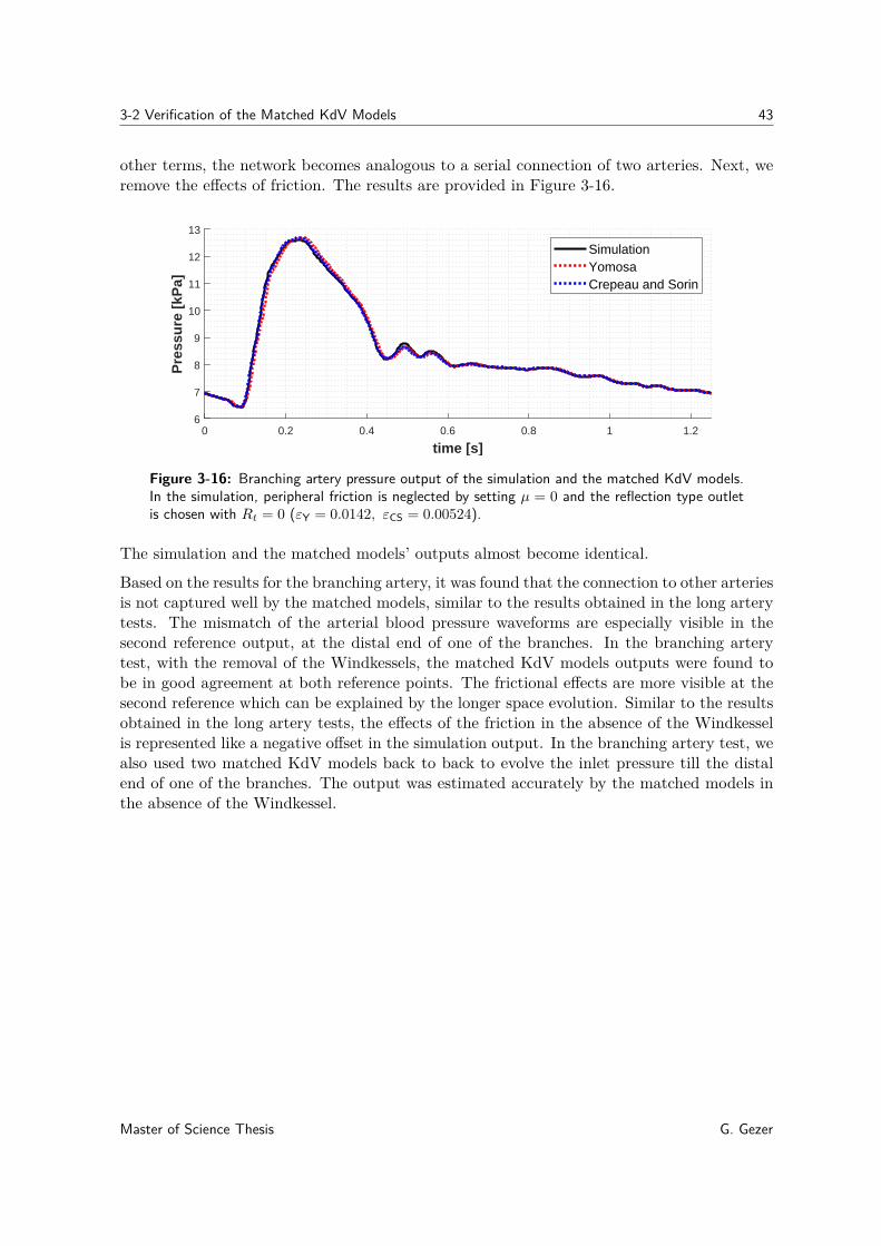
3-2 Verification of the Matched KdV Models 43
other terms, the network becomes analogous to a serial connection of two arteries. Next, weremove the effects of friction. The results are provided in Figure 3-16.
0 0.2 0.4 0.6 0.8 1 1.2
time [s]
6
7
8
9
10
11
12
13
Pre
ssu
re [
kPa]
SimulationYomosaCrepeau and Sorin
Figure 3-16: Branching artery pressure output of the simulation and the matched KdV models.In the simulation, peripheral friction is neglected by setting µ = 0 and the reflection type outletis chosen with Rt = 0 (εY = 0.0142, εCS = 0.00524).
The simulation and the matched models’ outputs almost become identical.
Based on the results for the branching artery, it was found that the connection to other arteriesis not captured well by the matched models, similar to the results obtained in the long arterytests. The mismatch of the arterial blood pressure waveforms are especially visible in thesecond reference output, at the distal end of one of the branches. In the branching arterytest, with the removal of the Windkessels, the matched KdV models outputs were found tobe in good agreement at both reference points. The frictional effects are more visible at thesecond reference which can be explained by the longer space evolution. Similar to the resultsobtained in the long artery tests, the effects of the friction in the absence of the Windkesselis represented like a negative offset in the simulation output. In the branching artery test, wealso used two matched KdV models back to back to evolve the inlet pressure till the distalend of one of the branches. The output was estimated accurately by the matched models inthe absence of the Windkessel.
Master of Science Thesis G. Gezer
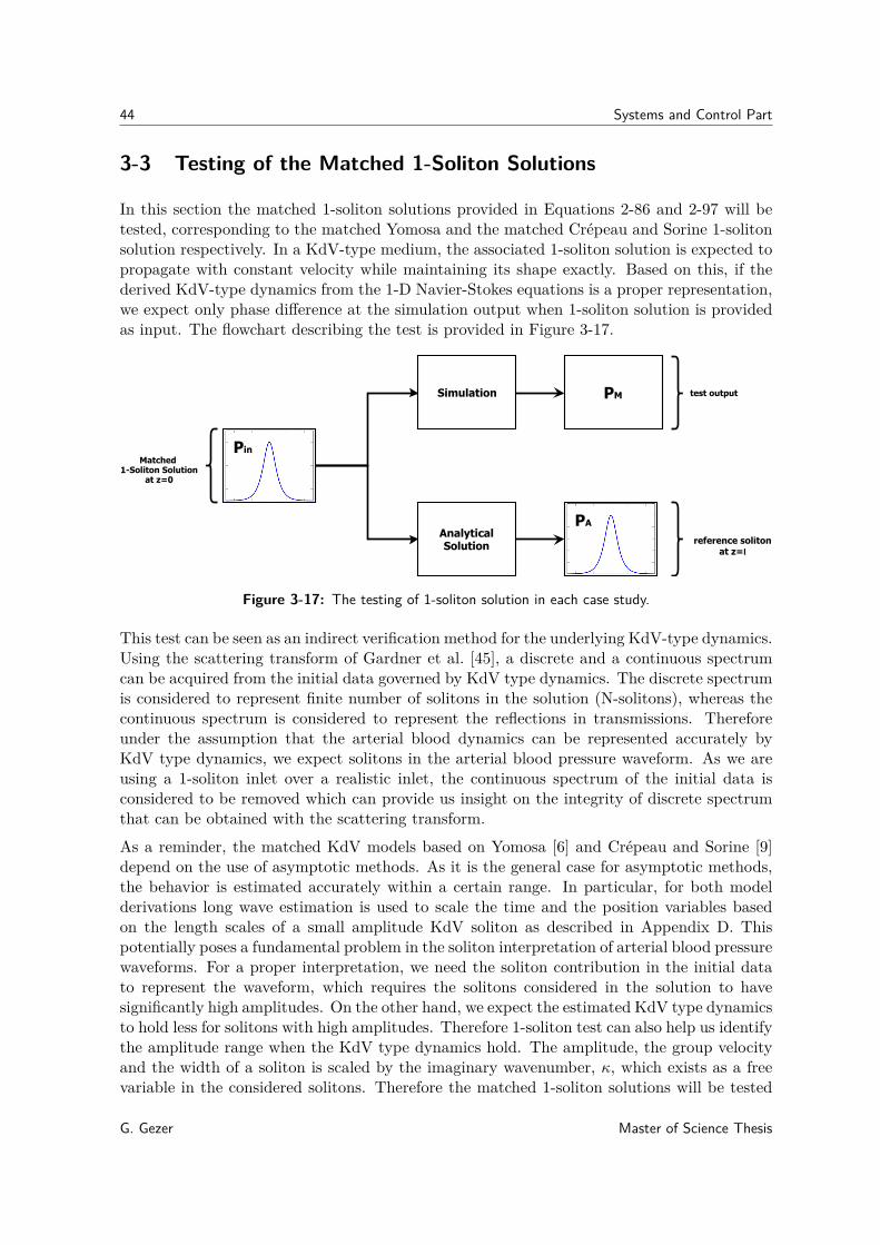
44 Systems and Control Part
3-3 Testing of the Matched 1-Soliton Solutions
In this section the matched 1-soliton solutions provided in Equations 2-86 and 2-97 will betested, corresponding to the matched Yomosa and the matched Crépeau and Sorine 1-solitonsolution respectively. In a KdV-type medium, the associated 1-soliton solution is expected topropagate with constant velocity while maintaining its shape exactly. Based on this, if thederived KdV-type dynamics from the 1-D Navier-Stokes equations is a proper representation,we expect only phase difference at the simulation output when 1-soliton solution is providedas input. The flowchart describing the test is provided in Figure 3-17.
Simulation
Matched 1Soliton Solution
at z=0
AnalyticalSolution reference soliton
at z=l
PM test output
Pin
PA
Figure 3-17: The testing of 1-soliton solution in each case study.
This test can be seen as an indirect verification method for the underlying KdV-type dynamics.Using the scattering transform of Gardner et al. [45], a discrete and a continuous spectrumcan be acquired from the initial data governed by KdV type dynamics. The discrete spectrumis considered to represent finite number of solitons in the solution (N-solitons), whereas thecontinuous spectrum is considered to represent the reflections in transmissions. Thereforeunder the assumption that the arterial blood dynamics can be represented accurately byKdV type dynamics, we expect solitons in the arterial blood pressure waveform. As we areusing a 1-soliton inlet over a realistic inlet, the continuous spectrum of the initial data isconsidered to be removed which can provide us insight on the integrity of discrete spectrumthat can be obtained with the scattering transform.
As a reminder, the matched KdV models based on Yomosa [6] and Crépeau and Sorine [9]depend on the use of asymptotic methods. As it is the general case for asymptotic methods,the behavior is estimated accurately within a certain range. In particular, for both modelderivations long wave estimation is used to scale the time and the position variables basedon the length scales of a small amplitude KdV soliton as described in Appendix D. Thispotentially poses a fundamental problem in the soliton interpretation of arterial blood pressurewaveforms. For a proper interpretation, we need the soliton contribution in the initial datato represent the waveform, which requires the solitons considered in the solution to havesignificantly high amplitudes. On the other hand, we expect the estimated KdV type dynamicsto hold less for solitons with high amplitudes. Therefore 1-soliton test can also help us identifythe amplitude range when the KdV type dynamics hold. The amplitude, the group velocityand the width of a soliton is scaled by the imaginary wavenumber, κ, which exists as a freevariable in the considered solitons. Therefore the matched 1-soliton solutions will be tested
G. Gezer Master of Science Thesis

3-3 Testing of the Matched 1-Soliton Solutions 45
within a range of κ. As the scaling also depends on the physical model parameters and thecoefficients of the matched KdV equations, the range for κ has to be adapted for each caseand between models.
In the simulation, the connection to other vessels and the peripheral friction will be included,as the clinical measurements are subject to the same effects. Same Pd and EC values used inthe previous section in the case studies. The analytical solution, PA, can be calculated easilyusing
PA = Ps(l, t), (3-6)
where Ps is the considered matched 1-soliton solution also used to calculate the pressure atthe inlet, Pin, such that
Pini = Ps(0, t). (3-7)
As the analytical solution is considered to be the reference behavior, the normalized error, ε,is defined as
ε = ||PM − PA||2||PA||2
. (3-8)
In Case III tests, only the first reference output at the end distal of the abdominal aorta isconsidered. This is based on the fact that the 1-soliton solution for the abdominal aorta is nota 1-soliton solution to the iliac arteries. This is explained by the dependence of the matchedKdV coefficients on physical model parameters.
Master of Science Thesis G. Gezer
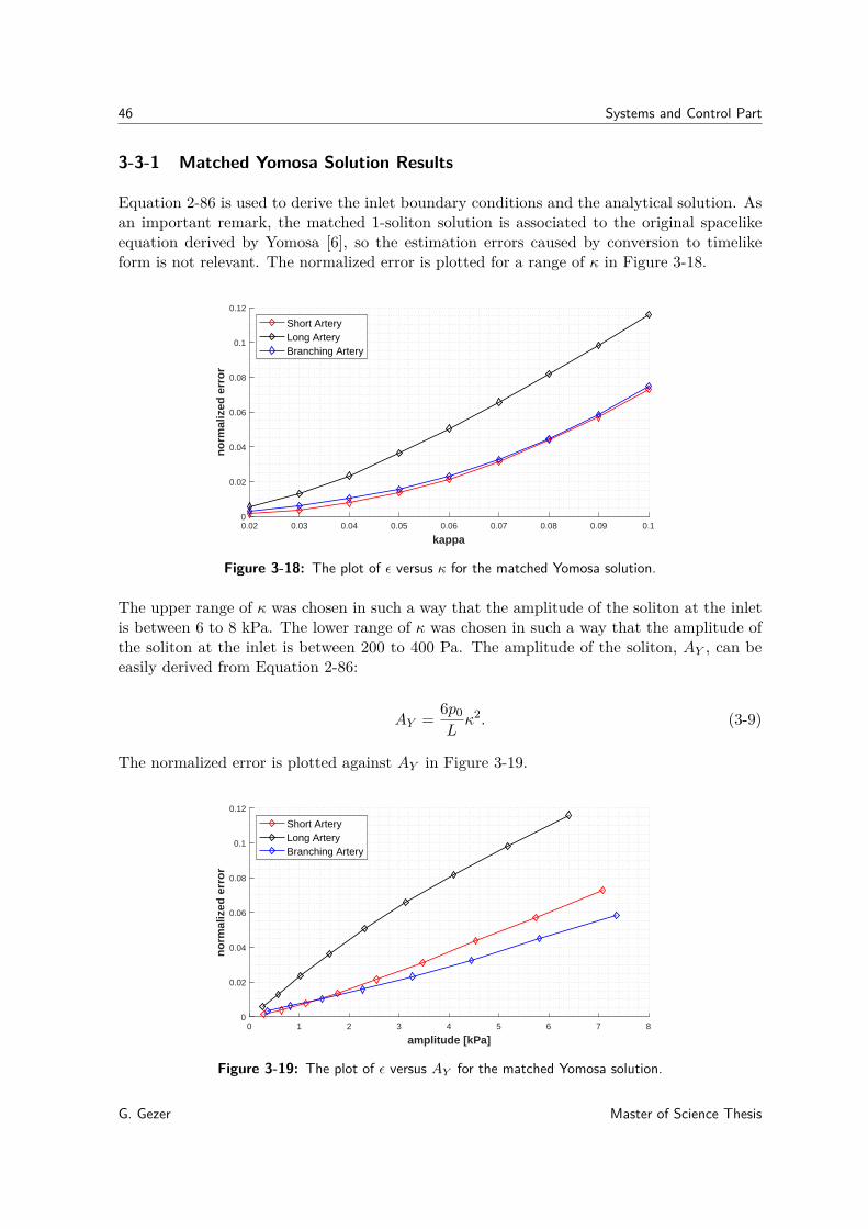
46 Systems and Control Part
3-3-1 Matched Yomosa Solution Results
Equation 2-86 is used to derive the inlet boundary conditions and the analytical solution. Asan important remark, the matched 1-soliton solution is associated to the original spacelikeequation derived by Yomosa [6], so the estimation errors caused by conversion to timelikeform is not relevant. The normalized error is plotted for a range of κ in Figure 3-18.
0.02 0.03 0.04 0.05 0.06 0.07 0.08 0.09 0.1
kappa
0
0.02
0.04
0.06
0.08
0.1
0.12
no
rmal
ized
err
or
Short ArteryLong ArteryBranching Artery
Figure 3-18: The plot of ε versus κ for the matched Yomosa solution.
The upper range of κ was chosen in such a way that the amplitude of the soliton at the inletis between 6 to 8 kPa. The lower range of κ was chosen in such a way that the amplitude ofthe soliton at the inlet is between 200 to 400 Pa. The amplitude of the soliton, AY , can beeasily derived from Equation 2-86:
AY = 6p0Lκ2. (3-9)
The normalized error is plotted against AY in Figure 3-19.
0 1 2 3 4 5 6 7 8
amplitude [kPa]
0
0.02
0.04
0.06
0.08
0.1
0.12
no
rmal
ized
err
or
Short ArteryLong ArteryBranching Artery
Figure 3-19: The plot of ε versus AY for the matched Yomosa solution.
G. Gezer Master of Science Thesis

3-3 Testing of the Matched 1-Soliton Solutions 47
Based on Figures 3-18 and 3-19, the normalized error is an increasing function of κ and AY .This is as expected due to long wave estimation. Although ε provides a measure of the matchbetween the analytical solution and the simulation output, it is also important to study thetime behavior. These differences are expected to be more visible in the long artery test as ε ishiger at the same AY compared to the other cases. The analytical solution and the simulationoutput for high amplitude soliton in long artery test is provided in Figure 3-20.
0 0.1 0.2 0.3 0.4 0.5 0.6 0.7 0.8 0.9 1
time [s]
6
7
8
9
10
11
12
13
pre
ssu
re [
kPa]
SimulationAnalytical
Figure 3-20: The comparison of the analytical solution and the simulation output in Case II(κ = 0.1).
Based on the plot, we see that the analytical solution is lagging. Furthermore the simula-tion output’s peak pressure is less compared to the analytical solution and there is a visibledeviation from soliton’s characteristic sech-squared profile. The analytical solution and thesimulation output for a lower amplitude soliton is provided in Figure 3-21.
0 0.1 0.2 0.3 0.4 0.5 0.6 0.7 0.8 0.9 1
time [s]
6.4
6.6
6.8
7
7.2
7.4
7.6
pre
ssu
re [
kPa]
SimulationAnalytical
Figure 3-21: The comparison of the analytical solution and the simulation output in Case II(κ = 0.04).
We see similar results in a smaller pressure scale compared to high amplitude soliton re-sults. However in comparison, the decrease of peak pressure and the phase difference is lessnoticeable.
Master of Science Thesis G. Gezer

48 Systems and Control Part
3-3-2 Matched Crépeau and Sorine Solution Results
Equation 2-97 is used to derive the inlet boundary conditions and the analytical solution. Asthe solution is associated to a timelike KdV equation, the scaling κ range is different fromthe tests done in the previous subsection. The normalized error is plotted for a range of κ inFigure 3-22.
100 200 300 400 500 600 700 800 900 1000 1100
kappa
0
0.005
0.01
0.015
0.02
0.025
0.03
0.035
0.04
0.045
no
rmal
ized
err
or
Short ArteryLong ArteryBranching Artery
Figure 3-22: The testing of 1-soliton solution in each case study.
The upper range of κ was chosen in such a way that the amplitude of the soliton at the inletis between 6 to 8 kPa. The lower range of κ was chosen in such a way that the amplitude ofthe soliton at the inlet is between 200 to 400 Pa. The amplitude of the soliton, ACS , can beeasily derived from Equation 2-97:
ACS = 3ρc0d2A0d1
κ2. (3-10)
The normalized error is plotted against ACS in Figure 3-23.
0 1 2 3 4 5 6 7 8
amplitude [kPa]
0
0.005
0.01
0.015
0.02
0.025
0.03
0.035
0.04
0.045
no
rmal
ized
err
or
Short ArteryLong ArteryBranching Artery
Figure 3-23: The plot of ε versus ACS for the matched Crépeau and Sorine solution.
G. Gezer Master of Science Thesis

3-3 Testing of the Matched 1-Soliton Solutions 49
Based on Figures 3-22 and 3-23, the normalized error is an increasing function of κ and AY .This is as expected due to long wave estimation. As an important remark, the tested inputsolitons were found to be very steep in nature, which is expected to cause numerical errorsin the simulation output as the provided time steps lead to misrepresentative discretizationof the input in the tested high κ range. The steepness of the matched Crépeau and Sorinesolutions are explained by the high nonlinear term scaling and low dispersion term scalingin the derived KdV equations. This problem could be solved by increasing the time stepsin the simulation file but this was found to cause stability problems. As the steepest solitonsolutions are tested in Case 2, this explains the difference of the error profile compared toother cases in the high κ range. Although ε provides a simplified measure of the matchbetween the analytical solution and the simulation output, it is also important to study thetime behavior. These differences are expected to be more visible in the long artery test butshort artery test will be considered to study time behavior for high κ instead due to thedescribed discretization problem. The analytical solution and the simulation output for highamplitude soliton in the short artery test is provided in Figure 3-24.
0 0.1 0.2 0.3 0.4 0.5 0.6 0.7 0.8 0.9 1
time [s]
4
6
8
10
12
14
16
pre
ssu
re [
kPa]
SimulationAnalytical
Figure 3-24: The comparison of the analytical solution and the simulation output in Case I(κ = 500).
Based on the plot, the simulation output’s peak pressure is less compared to the analyticalsolution and there is a visible deviation from soliton’s characteristic sech-squared profile.In fact the simulation output looks oscillatory, much like the response of an underdampedsystem. The analytical solution and the simulation output for a lower amplitude soliton inshort artery test is provided in Figure 3-25.
Master of Science Thesis G. Gezer

50 Systems and Control Part
0 0.1 0.2 0.3 0.4 0.5 0.6 0.7 0.8 0.9 1
time [s]
6.55
6.6
6.65
6.7
6.75
6.8
6.85
6.9p
ress
ure
[kP
a]
SimulationAnalytical
Figure 3-25: The comparison of the analytical solution and the simulation output in Case I(κ = 100).
The analytical solution and the simulation output are found to be in good agreement. To com-pare matched Crépeau and Sorine 1-soliton solution with matched Yomosa 1-soliton solution,the low amplitude soliton in long artery test is provided in Figure 3-26.
0 0.1 0.2 0.3 0.4 0.5 0.6 0.7 0.8 0.9 1
time [s]
6.5
6.6
6.7
6.8
6.9
pre
ssu
re [
kPa]
SimulationAnalytical
Figure 3-26: The comparison of the analytical solution and the simulation output in Case II(κ = 200).
The simulation output’s waveform is found to be similar compared to the results obtained inthe previous section (Figure 3-21). However unlike the results obtained for matched Yomosasolution, the phase difference between the analytical solution and the simulation is found tobe minimal. As a reminder, matched Crépeau and Sorine model was also found to outperformmatched Yomosa model in terms of phase estimation, when the realistic input were evolvedbased on the matched timelike KdV models (Figures 3-8, 3-9 and 3-10).
G. Gezer Master of Science Thesis

3-4 Nonlinear Fourier Analysis of Arterial Blood Pressure Waveform 51
3-4 Nonlinear Fourier Analysis of Arterial Blood Pressure Wave-form
In this test, the discrete spectrum of pressure at the inlet and at the outlet will be com-puted using the scattering transform proposed by Gardner et al. [45]. Unfamiliar readerscan find more information on scattering transform in Appendix C. The matched Yomosa andthe matched Crépeau and Sorine model will be used to derive the corresponding scatteringproblem parameter. Chebfun will be used for the computation of the spectrum. The discretespectrum of the input and the output will be compared and discussed. The flowchart of thistest is provided in Figure 3-27.
Pin Poutsimulation
discrete spectrum
discrete spectrum
compare
realisticinput
realisticoutput
Figure 3-27: The task description in each case study.
The scattering transform is analogous to a nonlinear generalization of Fourier transform. Inthe literature, the study of system behavior from such spectra is referred to as NonlinearFourier Analysis which is explained in detail in Osborne [46].
Consider the following timelike KdV equation:
P̂ + C1∂P̂
∂t+ C2P̂
∂P̂
∂t+ C3
∂3P̂
∂t3= 0. (3-11)
Soliton solutions to Equation 3-11 propagate in space and considered to be fixed in the frameξ = t − C1z − C3κ
2z, where κ is the imaginary wavenumber. The group velocity, v, of thesolitons then can be calculated based on ξ:
v(κ) = 1C1 + C3κ2 . (3-12)
Based on Gardner [45], the associated Schroedinger eigenvalue problem is
∂2Ψ∂t2
+ λP̂ (z0, t)Ψ + κ2Ψ = 0, (3-13)
where Ψ = Ψ(t) are the eigenfunctions associated with κ2 eigenvalues and λ is a measure ofnonlinearity to dispersion given by
Master of Science Thesis G. Gezer

52 Systems and Control Part
λ = C16C2
. (3-14)
As we will use Chebfun for the calculation of spectrum, the definition used for the scatteringproblem by Chebfun has to be considered as well. In particular, the quantumstates functionwill be used in Chebfun and based on the documentation the Schroedinger eigenvalue problemdefined as
h2∂2Ψ∂t2− V (z0, t)Ψ + κ̃2Ψ = 0, (3-15)
where h is considered to be the parameter instead of λ. Equation 3-13 can be transformedinto 3-15 by using the following transformations:
h =( 1λ
) 12, κ̃ = hκ, V (z0, t) = −P̂ (z0, t). (3-16)
The coefficients of the matched Yomosa model (2-91) and the matched Crépeau and Sorinemodel (Equation 2-99) can be substituted into Equation 3-11 to calculate h. Additionally theinitial data has to be reversed in sign and the scaling of the output wavenumbers should beconsidered in the spectrum calculations.
The number of negative eigenvalues included in the solution, N , will be finite, leading toN imaginary wavenumbers κ̃n and corresponding eigenfunctions Ψn. The calculated Ψn arenormalized wavefunctions so that
∫ ∞−∞||Ψn||2 dt = 1, ∀n ∈ {1, ..., N}. (3-17)
Ψn can be denormalized to original unit scaling using κ̃n [47]
ψn = 4hκ̃nΨ2n, (3-18)
where ψn is the denormalized wavefunction.
If the continuous spectrum is neglected, the initial data can be reconstructed using the de-normalized wavefunctions:
V (z0, t) ' Ve(t) =N∑n=1
ψn, (3-19)
where Ve is the estimate signal from the discrete spectrum. Based on Yomosa [6] and Crépeauand Sorine [9] 2 or 3 solitons can be used represent arterial blood pressure waveform. Basedon this hypothesis, in the case our calculations result with the calculation of more discretecomponents (N > 3), we will use the first 3 ψn to calculate Ve. As an important remark, thefirst 3 ψn correspond to the highest 3 κ̃n based on the calculation of the discrete spectrum so
G. Gezer Master of Science Thesis

3-4 Nonlinear Fourier Analysis of Arterial Blood Pressure Waveform 53
the most significant contributions will be included in the truncated estimates. The normalizederror between the arterial blood pressure waveform, PABP, and Ve is calculated as
ε = ||PABP − Ve||2||PABP||2
. (3-20)
3-4-1 Short Artery Results
First hY is calculated based on matched Yomosa model:
hY = 4.30. (3-21)
Using the calculated hY , we get 3 imaginary wavefunctions both for the input and the output.The denormalized wavefunctions and the arterial blood pressure waveform is provided inFigure 3-28.
0 0.2 0.4 0.6 0.8 1 1.2
time [s]
6
7
8
9
10
11
12
Pre
ssu
re [
kPa]
OUTPUT
ABP
1
2
3
0 0.2 0.4 0.6 0.8 1 1.2
time [s]
6
7
8
9
10
11
12
pre
ssu
re [
kPa]
INPUT
ABP
1
2
3
Figure 3-28: Calculated denormalized wavefunctions using matched Yomosa model for Case I.
Imaginary κ̃ values of the calculated input spectrum are given as
κ̃ ∈ {56.5, 39.0, 27.5}, (3-22)
Master of Science Thesis G. Gezer
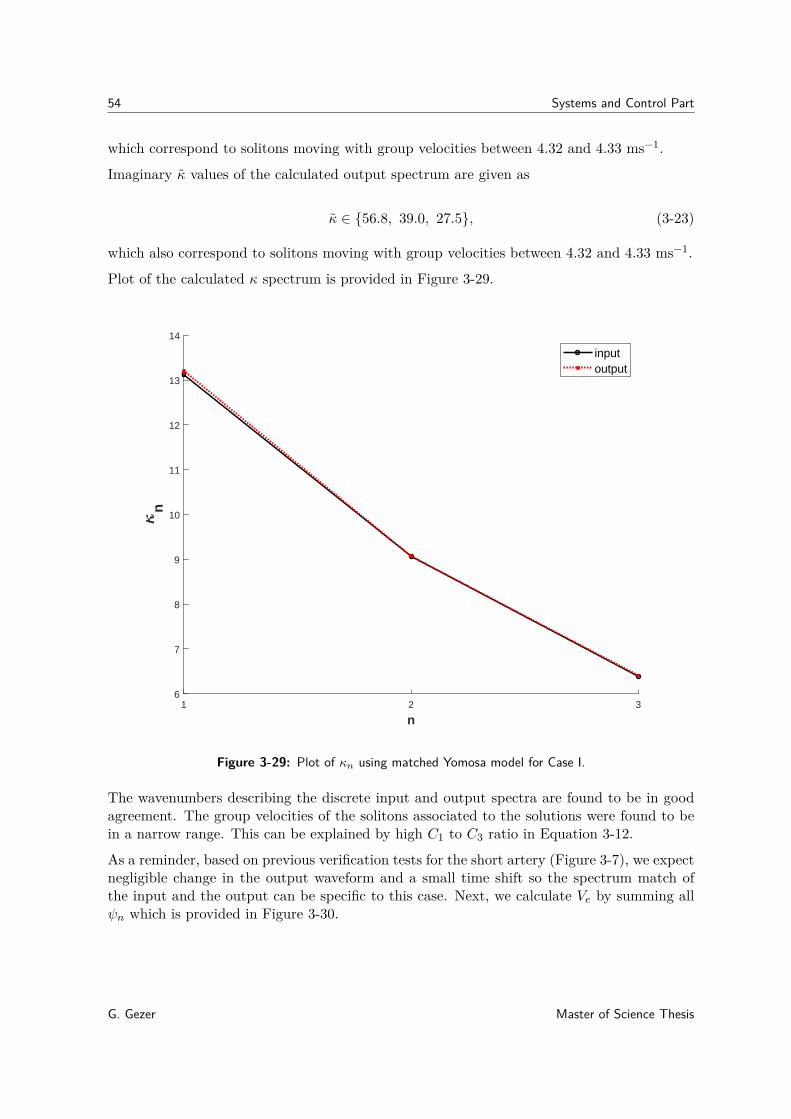
54 Systems and Control Part
which correspond to solitons moving with group velocities between 4.32 and 4.33 ms−1.
Imaginary κ̃ values of the calculated output spectrum are given as
κ̃ ∈ {56.8, 39.0, 27.5}, (3-23)
which also correspond to solitons moving with group velocities between 4.32 and 4.33 ms−1.
Plot of the calculated κ spectrum is provided in Figure 3-29.
1 2 3
n
6
7
8
9
10
11
12
13
14
n
inputoutput
Figure 3-29: Plot of κn using matched Yomosa model for Case I.
The wavenumbers describing the discrete input and output spectra are found to be in goodagreement. The group velocities of the solitons associated to the solutions were found to bein a narrow range. This can be explained by high C1 to C3 ratio in Equation 3-12.
As a reminder, based on previous verification tests for the short artery (Figure 3-7), we expectnegligible change in the output waveform and a small time shift so the spectrum match ofthe input and the output can be specific to this case. Next, we calculate Ve by summing allψn which is provided in Figure 3-30.
G. Gezer Master of Science Thesis

3-4 Nonlinear Fourier Analysis of Arterial Blood Pressure Waveform 55
0 0.2 0.4 0.6 0.8 1 1.2
time [s]
6
7
8
9
10
11
12
pre
ssu
re [
kPa]
OUTPUT
OriginalEstimate
0 0.2 0.4 0.6 0.8 1 1.2
time [s]
6
7
8
9
10
11
12p
ress
ure
[kP
a]INPUT
OriginalEstimate
Figure 3-30: The estimate of ABP waveform from the discrete spectrum using matched Yomosamodel for Case I.
The normalized errors associated to the estimates are calculated as
εin = 0.237, εout = 0.229. (3-24)
Based on Figure 3-30, the reconstruction of the waveform based on the matched Yomosamodel results with a simplified waveform that captures the main variations in the originalwaveform. However the minor variations of the original waveform are not captured well inthe reconstructed signal.
Considering the soliton interpretation of the arterial blood pressure waveform and referringto Figure 3-28, ψ1 is considered to represent the systolic phenomena in which the wave groupvelocity and amplitude is the highest. ψ3 is considered to represent the diastolic phenomenain which the wave group velocity and the amplitude is lowest. ψ2 can be associated to anintermediate wave which seems to be dominant following the closing of the aortic valve.
Next hCS is calculated based on matched Crépeau and Sorine model:
hCS = 0.226. (3-25)
Master of Science Thesis G. Gezer

56 Systems and Control Part
Using the calculated hCS , we get 71 imaginary wavefunctions both for the input and theoutput. This is explained by the smallness of hCS as N included in the solution is a decreasingfunction of h used for analysis. However the results contradict with Crépeau and Sorine andcoworkers’ results [9, 11] as 3 solitons chosen from such spectrum is not expected to representthe waveform well. The first three denormalized wavefunctions and the arterial blood pressurewaveform are provided in Figure 3-31.
0 0.2 0.4 0.6 0.8 1 1.2
time [s]
6
7
8
9
10
11
12
Pre
ssu
re [
kPa]
OUTPUT
ABP
1
2
3
0 0.2 0.4 0.6 0.8 1 1.2
time [s]
6
7
8
9
10
11
12
pre
ssu
re [
kPa]
INPUT
ABP
1
2
3
Figure 3-31: Calculated first 3 denormalized wavefunctions using matched Crépeau and Sorinemodel for Case I.
Considering the fact that the first three wavefunctions belong to the highest amplitude andgroup velocity solitons, the rest of the denormalized wavefunctions will have even smallercontribution. Next, we calculate Ve by summing the first 3 ψn which is provided in Figure3-32.
The normalized errors associated to the estimates are calculated as
εin = 0.892, εout = 0.891. (3-26)
The estimates do not represent the original waveform. The results indicate that matchedCrépeau and Sorine model rather explains a soliton interpretation of the arterial blood pres-sure waveform corresponding to the transmission of many small amplitude solitons. Referring
G. Gezer Master of Science Thesis

3-4 Nonlinear Fourier Analysis of Arterial Blood Pressure Waveform 57
0 0.2 0.4 0.6 0.8 1 1.2
time [s]
6
7
8
9
10
11
12
pre
ssu
re [
kPa]
OUTPUT
OriginalEstimate
0 0.2 0.4 0.6 0.8 1 1.2
time [s]
6
7
8
9
10
11
12p
ress
ure
[kP
a]INPUT
OriginalEstimate
Figure 3-32: The estimate of ABP waveform from the discrete spectrum using matched Crépeauand Sorine model for Case I using the first 3 denormalized wavefunctions.
back to the previous results, the 1-soliton solutions to matched Crépeau and Sorine modelwere found to be too steep, which in a way requires many solitons in the solution to representthe entire waveform. As an example, in Figure 3-33 all 71 denormalized wavefunctions areused for the estimation of Ve.
Master of Science Thesis G. Gezer

58 Systems and Control Part
0 0.2 0.4 0.6 0.8 1 1.2
time [s]
6
7
8
9
10
11
12
pre
ssu
re [
kPa]
OUTPUT
OriginalEstimate
0 0.2 0.4 0.6 0.8 1 1.2
time [s]
6
7
8
9
10
11
12p
ress
ure
[kP
a]INPUT
OriginalEstimate
Figure 3-33: The estimate of ABP waveform from the discrete spectrum based on matchedCrépeau and Sorine model for Case I using all 71 denormalized wavefunctions.
The normalized errors associated to the estimates are calculated as
εin = 0.00458, εout = 0.00876. (3-27)
The estimate and the original signal seem to be identical but this can alternatively be seenas an overfitting problem. The estimate error between the reconstructed signal from thediscrete spectrum and the original signal, is a decreasing function of h. As a consequence, if his chosen smaller than what it should be based on the physics of the medium, the continuoussolution would be forced to become negligible and the scattering data would be representingunphysical phenomena. The process can be seen analogous to modeling a signal using sech-squared functions - as long as we include enough of them in the solution, the estimation errorwill vanish.
Plot of the calculated κ spectrum is provided in Figure 3-34.
G. Gezer Master of Science Thesis

3-4 Nonlinear Fourier Analysis of Arterial Blood Pressure Waveform 59
10 20 30 40 50 60 70
n
0
10
20
30
40
50
60
70
n
inputoutput
Figure 3-34: Plot of κn of matched Crépeau and Sorine model for Case I.
The input and the output spectrum are found to be in good agreement. Soliton solutionsassociated to the input and the output were found to have group velocities between 5.15to 5.38 m−1. Based on Figure 3-34, we see change of profile after n = 16. Following thisintuition, the fastest 16 solitons are grouped together to estimate a systolic component whichis given in Figure 3-35.
Master of Science Thesis G. Gezer
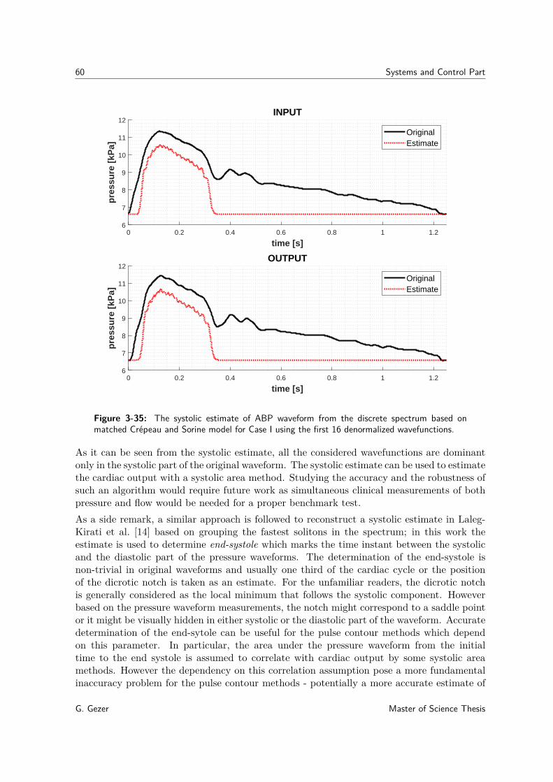
60 Systems and Control Part
0 0.2 0.4 0.6 0.8 1 1.2
time [s]
6
7
8
9
10
11
12
pre
ssu
re [
kPa]
OUTPUT
OriginalEstimate
0 0.2 0.4 0.6 0.8 1 1.2
time [s]
6
7
8
9
10
11
12p
ress
ure
[kP
a]INPUT
OriginalEstimate
Figure 3-35: The systolic estimate of ABP waveform from the discrete spectrum based onmatched Crépeau and Sorine model for Case I using the first 16 denormalized wavefunctions.
As it can be seen from the systolic estimate, all the considered wavefunctions are dominantonly in the systolic part of the original waveform. The systolic estimate can be used to estimatethe cardiac output with a systolic area method. Studying the accuracy and the robustness ofsuch an algorithm would require future work as simultaneous clinical measurements of bothpressure and flow would be needed for a proper benchmark test.As a side remark, a similar approach is followed to reconstruct a systolic estimate in Laleg-Kirati et al. [14] based on grouping the fastest solitons in the spectrum; in this work theestimate is used to determine end-systole which marks the time instant between the systolicand the diastolic part of the pressure waveforms. The determination of the end-systole isnon-trivial in original waveforms and usually one third of the cardiac cycle or the positionof the dicrotic notch is taken as an estimate. For the unfamiliar readers, the dicrotic notchis generally considered as the local minimum that follows the systolic component. Howeverbased on the pressure waveform measurements, the notch might correspond to a saddle pointor it might be visually hidden in either systolic or the diastolic part of the waveform. Accuratedetermination of the end-sytole can be useful for the pulse contour methods which dependon this parameter. In particular, the area under the pressure waveform from the initialtime to the end systole is assumed to correlate with cardiac output by some systolic areamethods. However the dependency on this correlation assumption pose a more fundamentalinaccuracy problem for the pulse contour methods - potentially a more accurate estimate of
G. Gezer Master of Science Thesis

3-4 Nonlinear Fourier Analysis of Arterial Blood Pressure Waveform 61
the end-systole might work as good as a rough estimate in terms of global flow estimation.
Major differences were found between matched Yomosa and Crépeau and Sorine models inthe discrete spectrum analysis. Nonlinear Fourier analysis based on Matched Yomosa modelreturned 3 high amplitude solitons propagating relatively with similar group velocities, specif-ically between 4.32 and 4.33 ms−1. Nonlinear Fourier analysis based on Matched Crépeauand Sorine model returned 71 low-amplitude solitons propagating relatively with more diversegroup velocities, specifically between 5.15 and 5.38 ms−1.
3-4-2 Long Artery Results
First hY is calculated based on the matched Yomosa model:
hY = 2.07. (3-28)
Using the calculated hY , we get 8 and 7 imaginary wavefunctions for the input and the outputrespectively. The first 3 denormalized wavefunctions and the arterial blood pressure waveformis provided in Figure 3-36.
0 0.2 0.4 0.6 0.8 1 1.2
time [s]
6
8
10
12
14
Pre
ssu
re [
kPa]
OUTPUT
ABP
1
2
3
0 0.2 0.4 0.6 0.8 1 1.2
time [s]
6
7
8
9
10
11
12
pre
ssu
re [
kPa]
INPUT
ABP
1
2
3
Figure 3-36: Calculated first three denormalized wavefunctions using matched Yomosa modelfor Case II.
Master of Science Thesis G. Gezer

62 Systems and Control Part
Imaginary κ̃ values of the calculated input spectrum are given as
κ̃ ∈ {63.6, 52.9, 43.8, 37.3, 32.9, 27.4, 20.6, 6.34}. (3-29)
which correspond to solitons moving with group velocities between 3.31 and 3.34 ms−1.
Imaginary κ̃ values of the calculated output spectrum are given as
κ̃ ∈ {71.6, 58.2, 43.8, 36.7, 32.0, 25.5, 17.7}. (3-30)
which correspond to solitons moving with group velocities between 3.32 and 3.34 ms−1.
Plot of the calculated κ spectrum is provided in Figure 3-37.
1 2 3 4 5 6 7 8
n
0
5
10
15
20
25
30
35
n
inputoutput
Figure 3-37: Plot of κn using matched Yomosa model for Case II.
The first two wavenumbers for the input and the output are found to be higher in the output.The rest of the wavenumbers are found to be in good agreement. As a reminder, based onprevious verification tests for the long artery (Figure 3-8), the simulation output had highervalues in the systolic portion of the waveform whereas the diastolic portion was found tobe in good agreement. The calculated imaginary wavenumbers provide us a similar insight,as the high wavenumbers are associated to the systolic portion of the wavenumber, whereasthe lower ones are associated to the diastolic portion. Examining Figure 3-36, in the input
G. Gezer Master of Science Thesis

3-4 Nonlinear Fourier Analysis of Arterial Blood Pressure Waveform 63
waveform we see the first two wavefunctions are in the systolic portion, whereas the third oneis located in the portion associated to the closing of the aortic valve. In the output waveform,the third wavefunction is absorbed into the systolic portion seemingly moving backward.This can be explained steepening which can be addressed by connections to other vesselsbut not properly by matched KdV model based on previous results for KdV type dynamicsverification. Additionally based on test the results of the associated 1-soliton solutions, weexpect low amplitude solitons at the inlet to be more preserved at the outlet, which can beseen from the agreement of lower κ̃ values.
Next, we calculate Ve by summing the first 3 ψn which is provided in Figure 3-38.
0 0.2 0.4 0.6 0.8 1 1.2
time [s]
6
8
10
12
14
pre
ssu
re [
kPa]
OUTPUT
OriginalEstimate
0 0.2 0.4 0.6 0.8 1 1.2
time [s]
6
7
8
9
10
11
12
pre
ssu
re [
kPa]
INPUT
OriginalEstimate
Figure 3-38: The estimate of ABP waveform from the discrete spectrum using matched Yomosamodel for Case II using the first 3 denormalized wavefunctions.
The normalized errors associated to the estimates are calculated as
εin = 0.357, εout = 0.412. (3-31)
Based on Figure 3-38, the reconstruction of the waveform using the first wavefunctions yield agood representation only in the systolic portion as discussed before, especially at the output.The estimate can be improved by including all the calculated denormalized wavefunctions,which is shown in Figure 3-39.
Master of Science Thesis G. Gezer

64 Systems and Control Part
0 0.2 0.4 0.6 0.8 1 1.2
time [s]
6
8
10
12
14
pre
ssu
re [
kPa]
OUTPUT
OriginalEstimate
0 0.2 0.4 0.6 0.8 1 1.2
time [s]
6
7
8
9
10
11
12p
ress
ure
[kP
a]INPUT
OriginalEstimate
Figure 3-39: The estimate of ABP waveform from the discrete spectrum using matched Yomosamodel for Case II using all denormalized wavefunctions.
The normalized errors associated to the new estimates are calculated as
εin = 0.0632, εout = 0.0847. (3-32)
The estimate error are low, which can be associated to the reduce value of hY . As animportant remark, the difference of hY value in the short and the long artery case, changethe interpretation of the same waveform as the input of the long artery test is assigned asthe short artery test, which essentially were found to have different κ spectra with differentgroup velocities between the cases. This is as expected as the analysis method depends ondifferent dynamics. The finding also suggests that a global nonlinear Fourier analysis mightbe problematic using the matched Yomosa model as the local interpretation of the samewaveform differs a lot between different vessels.Next hCS is calculated based on matched Crépeau and Sorine model:
hCS = 0.226. (3-33)
Using the calculated hCS , we get 69 and 71 imaginary wavefunctions for the input and theoutput respectively. It should be pointed out that the calculated hCS has the same value in
G. Gezer Master of Science Thesis

3-4 Nonlinear Fourier Analysis of Arterial Blood Pressure Waveform 65
the short artery test. This is a promising result for global nonlinear Fourier analysis, as theparameter was found to be invariant between different arteries. Based on the results obtainedfrom the short artery test, discussion based on the first 3 solitons are avoided as the first 3solitons out of many were not found to be good representatives for the matched Crépeau andSorine model.
Plot of the calculated κ spectrum is provided in Figure 3-40.
10 20 30 40 50 60 70
n
0
10
20
30
40
50
60
70
80
n
inputoutput
Figure 3-40: Plot of κn of matched Crépeau and Sorine model for Case II.
Based on the plot, the imaginary wavenumber spectrum varies significantly in the input andthe output spectrum. As the output pressure is calculated based on the simulation model, it isimportant to consider the results obtained in the long artery KdV type dynamics verificationtest (Figure 3-8). The simulation output had increased pressure in the systolic part, which wasexplained in the context of steepening caused by connection to the other vessels and there wasa general pressure reduction in the output waveform due to the inclusion of friction. Figure3-40 provides us a similar insight, as in general κ values of the output are smaller with respectto the input except for the highest κ values which were found to increase at the output. Asa reminder, the high κ values are associated to the systolic part of the waveform and the lowκ values are associated to the diastolic part so by inspecting Figure 3-40 we can extrapolatethe differences in time behavior and vice versa.
The group velocities of the input solitons were found between 5.16 and 5.38 ms−1 which
Master of Science Thesis G. Gezer

66 Systems and Control Part
matches the group velocities found for the output in the short artery test. The group velocitiesof the output solitons were found between 5.16 and 5.45 ms−1.Next we calculate Ve based on all calculated denormalized wavefunctions which is providedin Figure 3-41.
0 0.2 0.4 0.6 0.8 1 1.2
time [s]
6
8
10
12
14
pre
ssu
re [
kPa]
OUTPUT
OriginalEstimate
0 0.2 0.4 0.6 0.8 1 1.2
time [s]
6
7
8
9
10
11
12
pre
ssu
re [
kPa]
INPUT
OriginalEstimate
Figure 3-41: The estimate of ABP waveform from the discrete spectrum based on matchedCrépeau and Sorine model for Case II using all calculated denormalized wavefunctions.
The normalized errors associated to the estimates are calculated as
εin = 0.0174, εout = 0.00421. (3-34)
As many solitons are included in the solution, the reconstruction error is found to be minimal.Next we only consider the first 16 wavefunctions in the reconstruction to estimate a systoliccomponent which is provided in Figure 3-42.Like the results obtained in the short artery analysis, the first 16 wavefunctions are found to bedominant in the systolic portion of the waveform. As discussed in the short artery analysis,the systolic estimate can be potentially used to estimate global flow and/or to determineend-systole.Major differences were found between matched Yomosa and Crépeau and Sorine models in thediscrete spectrum analysis in the long artery case. The analysis based on matched Yomosa
G. Gezer Master of Science Thesis

3-4 Nonlinear Fourier Analysis of Arterial Blood Pressure Waveform 67
0 0.2 0.4 0.6 0.8 1 1.2
time [s]
6
8
10
12
14
pre
ssu
re [
kPa]
OUTPUT
OriginalEstimate
0 0.2 0.4 0.6 0.8 1 1.2
time [s]
6
7
8
9
10
11
12p
ress
ure
[kP
a]INPUT
OriginalEstimate
Figure 3-42: The systolic estimate of ABP waveform from the discrete spectrum based onmatched Crépeau and Sorine model for Case II using the first 16 denormalized wavefunctions.
model resulted in a different spectrum for the same waveform. In contrast, analysis based onmatched Crépeau and Sorine model resulted with identical spectrum for the same waveform.However based on the KdV-type dynamics verification results for the long artery, the matchedCrépeau and Sorine model was found inadequate to model the effects of connection to theother vessels which can be also observed in the differing κ spectrum of the input and theoutput. Although the matched Crépeau and Sorine model was found compatible for globalanalysis, the mismatch in the simulation and the matched Crépeau and Sorine dynamics fromthe dynamics verification test suggest that information obtained from the analysis might berepresenting mathematical phenomena rather than physical phenomena.
Master of Science Thesis G. Gezer

68 Systems and Control Part
3-4-3 Branching Artery Results
First hY is calculated based on the matched Yomosa model:
hY = 2.86. (3-35)
Using the calculated hY , we get 5 imaginary wavefunctions both for the input and the output.The first 3 denormalized wavefunctions and the arterial blood pressure waveform is providedin Figure 3-43.
0 0.2 0.4 0.6 0.8 1 1.2
time [s]
6
8
10
12
14
Pre
ssu
re [
kPa]
OUTPUT
ABP
1
2
3
0 0.2 0.4 0.6 0.8 1 1.2
time [s]
6
8
10
12
14
pre
ssu
re [
kPa]
INPUT
ABP
1
2
3
Figure 3-43: Calculated first 3 denormalized wavefunctions using matched Yomosa model forCase III.
Imaginary κ̃ values of the calculated input spectrum are given as
κ̃ ∈ {70.0, 51.5, 37.8, 31.5, 22.3}, (3-36)
which correspond to solitons moving with group velocities between 5.30 and 5.32 ms−1.
Imaginary κ̃ values of the calculated output spectrum are given as
κ̃ ∈ {73.1, 51.4, 37.7, 31.0, 21.4}. (3-37)
G. Gezer Master of Science Thesis

3-4 Nonlinear Fourier Analysis of Arterial Blood Pressure Waveform 69
which correspond to solitons moving with group velocities between 5.30 and 5.33 ms−1.
The wavenumbers for the input and the output are found to be in good agreement exceptthe first one which is increased in the output. As a reminder, based on previous verificationtests for the branching artery (Figure 3-11), we expect negligible change in the first referenceoutput waveform except an increase in the systolic portion which can be explained by theincrease in the first wavenumber. Next, we calculate Ve by summing the first three ψn whichis provided in Figure 3-44.
0 0.2 0.4 0.6 0.8 1 1.2
time [s]
6
8
10
12
14
pre
ssu
re [
kPa]
OUTPUT
OriginalEstimate
0 0.2 0.4 0.6 0.8 1 1.2
time [s]
6
8
10
12
14
pre
ssu
re [
kPa]
INPUT
OriginalEstimate
Figure 3-44: The estimate of ABP waveform from the discrete spectrum using matched Yomosamodel for Case III using the first 3 denormalized wavefunctions.
The normalized errors associated to the estimates are calculated as
εin = 0.245, εout = 0.260. (3-38)
The estimate can be improved by including all the calculated denormalized wavefunctions,which is shown in Figure 3-45.
Master of Science Thesis G. Gezer
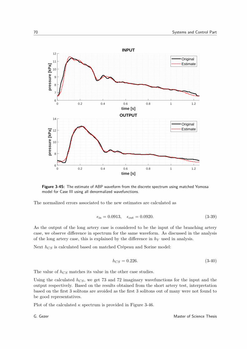
70 Systems and Control Part
0 0.2 0.4 0.6 0.8 1 1.2
time [s]
6
8
10
12
14
pre
ssu
re [
kPa]
OUTPUT
OriginalEstimate
0 0.2 0.4 0.6 0.8 1 1.2
time [s]
6
7
8
9
10
11
12p
ress
ure
[kP
a]INPUT
OriginalEstimate
Figure 3-45: The estimate of ABP waveform from the discrete spectrum using matched Yomosamodel for Case III using all denormalized wavefunctions.
The normalized errors associated to the new estimates are calculated as
εin = 0.0913, εout = 0.0920. (3-39)
As the output of the long artery case is considered to be the input of the branching arterycase, we observe difference in spectrum for the same waveform. As discussed in the analysisof the long artery case, this is explained by the difference in hY used in analysis.
Next hCS is calculated based on matched Crépeau and Sorine model:
hCS = 0.226. (3-40)
The value of hCS matches its value in the other case studies.
Using the calculated hCS , we get 73 and 72 imaginary wavefunctions for the input and theoutput respectively. Based on the results obtained from the short artery test, interpretationbased on the first 3 solitons are avoided as the first 3 solitons out of many were not found tobe good representatives.
Plot of the calculated κ spectrum is provided in Figure 3-46.
G. Gezer Master of Science Thesis

3-4 Nonlinear Fourier Analysis of Arterial Blood Pressure Waveform 71
10 20 30 40 50 60 70
n
0
10
20
30
40
50
60
70
80
90
n
inputoutput
Figure 3-46: Plot of κn of matched Crépeau and Sorine model for Case III.
The input and output spectra were found to be in good agreement. We observe increase inthe highest κ values at the output which can be explained by the steepening behavior causedby the connection to the other vessels.
The group velocities of the input solitons were found between 5.16 and 5.45 ms−1 whichmatches the group velocities found for the output in the short artery test. The group velocitiesof the output solitons were found to be between 5.16 and 5.51 ms−1.
Next we calculate Ve based on all calculated denormalized wavefunctions which is providedin Figure 3-47.
Master of Science Thesis G. Gezer

72 Systems and Control Part
0 0.2 0.4 0.6 0.8 1 1.2
time [s]
6
8
10
12
14
pre
ssu
re [
kPa]
OUTPUT
OriginalEstimate
0 0.2 0.4 0.6 0.8 1 1.2
time [s]
6
8
10
12
14p
ress
ure
[kP
a]INPUT
OriginalEstimate
Figure 3-47: The estimate of ABP waveform from the discrete spectrum based on matchedCrépeau and Sorine model for Case III using all calculated denormalized wavefunctions.
The normalized errors associated to the estimates are calculated as
εin = 0.0198, εout = 0.0174. (3-41)
The reconstruction error is found to be minimal.
Next we only consider the first 16 wavefunctions in the reconstruction to estimate a systoliccomponent which is provided in Figure 3-48.
G. Gezer Master of Science Thesis

3-4 Nonlinear Fourier Analysis of Arterial Blood Pressure Waveform 73
0 0.2 0.4 0.6 0.8 1 1.2
time [s]
6
8
10
12
14
pre
ssu
re [
kPa]
OUTPUT
OriginalEstimate
0 0.2 0.4 0.6 0.8 1 1.2
time [s]
6
8
10
12
14p
ress
ure
[kP
a]INPUT
OriginalEstimate
Figure 3-48: The systolic estimate of ABP waveform from the discrete spectrum based onmatched Crépeau and Sorine model for Case III using the first 16 denormalized wavefunctions.
Like the results obtained in the analysis of the previous cases, the first 16 wavefunctions arefound to be dominant in the systolic portion of the waveform. As discussed in the shortartery analysis, the systolic estimate can be potentially used to estimate global flow and/orto determine end-systole.
As the scattering transform parameter was found to be invariant between cases, we also repeatthe analysis based on matched Crépeau and Sorine at the outlet of the branches. In particular,the input corresponds to the inlet of the abdominal aorta and the output corresponds to theoutlet of one of the iliac arteries in the following tests.
Using the same hCS , we get 73 and 71 imaginary wavefunctions for the input and the outputrespectively.
Plot of the calculated κ spectrum is provided in Figure 3-49.
Master of Science Thesis G. Gezer

74 Systems and Control Part
10 20 30 40 50 60 70
n
0
10
20
30
40
50
60
70
80
90
n
inputoutput
Figure 3-49: Plot of κn of matched Crépeau and Sorine model for Case III.
The differences between the input and the output spectrum are found to be greater, comparedto the results obtained for the first reference pressure in the same case study. Similarly, weobserve increase in the highest κ values at the output which can be explained steepeningbehavior caused by the connection to the other vessels.
The group velocities of the output solitons were found between 5.16 and 5.55 ms−1.
Next we calculate Ve based on all calculated denormalized wavefunctions which is providedin Figure 3-50.
G. Gezer Master of Science Thesis

3-4 Nonlinear Fourier Analysis of Arterial Blood Pressure Waveform 75
0 0.2 0.4 0.6 0.8 1 1.2
time [s]
6
8
10
12
14
pre
ssu
re [
kPa]
OUTPUT
OriginalEstimate
0 0.2 0.4 0.6 0.8 1 1.2
time [s]
6
8
10
12
14p
ress
ure
[kP
a]INPUT
OriginalEstimate
Figure 3-50: The estimate of ABP waveform from the discrete spectrum based on matchedCrépeau and Sorine model for Case III using all calculated denormalized wavefunctions.
The normalized errors associated to the estimates are calculated as
εin = 0.0198, εout = 0.0174. (3-42)
The reconstruction error is found to be minimal.
Next we only consider the first 16 wavefunctions in the reconstruction to estimate a systoliccomponent which is provided in Figure 3-51.
Master of Science Thesis G. Gezer
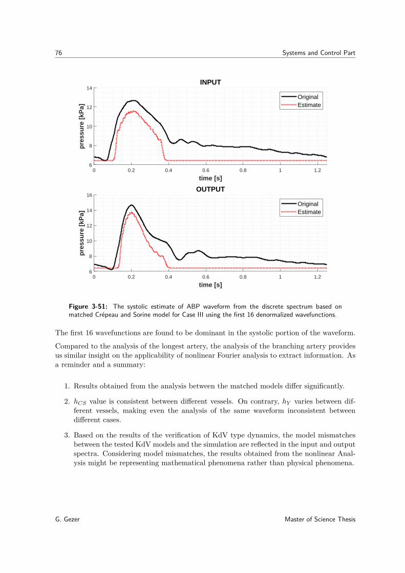
76 Systems and Control Part
0 0.2 0.4 0.6 0.8 1 1.2
time [s]
6
8
10
12
14
16
pre
ssu
re [
kPa]
OUTPUT
OriginalEstimate
0 0.2 0.4 0.6 0.8 1 1.2
time [s]
6
8
10
12
14p
ress
ure
[kP
a]INPUT
OriginalEstimate
Figure 3-51: The systolic estimate of ABP waveform from the discrete spectrum based onmatched Crépeau and Sorine model for Case III using the first 16 denormalized wavefunctions.
The first 16 wavefunctions are found to be dominant in the systolic portion of the waveform.
Compared to the analysis of the longest artery, the analysis of the branching artery providesus similar insight on the applicability of nonlinear Fourier analysis to extract information. Asa reminder and a summary:
1. Results obtained from the analysis between the matched models differ significantly.
2. hCS value is consistent between different vessels. On contrary, hY varies between dif-ferent vessels, making even the analysis of the same waveform inconsistent betweendifferent cases.
3. Based on the results of the verification of KdV type dynamics, the model mismatchesbetween the tested KdV models and the simulation are reflected in the input and outputspectra. Considering model mismatches, the results obtained from the nonlinear Anal-ysis might be representing mathematical phenomena rather than physical phenomena.
G. Gezer Master of Science Thesis

Chapter 4
Conclusion
Biomechanical Design Part addresses the clinical importance of modeling arterial blood pres-sure waveforms in the context of improving non-invasive cardiac output measurements andincludes the derivation of dynamics from the basics of fluid motion to the two arterial bloodpressure KdV models proposed by Yomosa [6] and Crépeau and Sorine [9]. Using the nor-malization steps provided in both papers, we derive KdV equation coefficients for the originalpressure variable. Yomosa’s spacelike KdV equation is converted into timelike form to addressspace evolution in an artery instead of time evolution, as clinical pressure measurements aredone at fixed locations in continuous time. Using the KdV equation in the original pressurevariable from Crépeau and Sorine, the corresponding 1-soliton solution for pressure is alsoderived. The explicit and underlying assumptions of both works are explained in detail. Ad-ditional assumptions on the physical parameters are made to make both models consistentwith the simulation software, openBF [10], resulting with the matched KdV models and theassociated matched 1-soliton solutions.
Systems and Control Part includes the description of the case studies, verification of bothmatched models’ KdV type dynamics and associated 1-soliton solutions, and analysis of arte-rial blood pressure waveform using scattering transform. The case studies comprise of a shortartery, a long artery and a branching artery network which are considered to be the sectionsof a simplified arterial network from aortic root to the distal end of both iliac arteries.
In the KdV type dynamics verification tests, a realistic pressure waveform is considered asthe input for the simplified arterial network and the pressure output is calculated based onthe matched KdV equations. The outputs of the matched KdV models are compared to thesimulation output to evaluate fits. Both matched KdV model outputs were found to be ingood agreement with the simulation output in the short artery case. In the long artery and inthe branching artery cases, the systolic parts of both matched KdV model outputs were foundto differ from the simulation output. The matched KdV models were found to be inadequateat modeling the steepening phenomena, when the tested vessel or network is assumed to beconnected to the other vessels. The effects of including peripheral friction were found to besmall but still relevant for the mismatches. Overall the matched Crépeau and Sorine modeloutput was found to a better fit for the simulation output in all case studies.
Master of Science Thesis G. Gezer

78 Conclusion
In the 1-soliton solutions test, the matched 1-soliton solution of Yomosa [6] and the matched1-soliton solution derived based on Crépeau and Sorine [9], were used as an inlet to thesimulation to test soliton propagation. The analytical solution and the simulation outputwere compared for both models and it was found that the 1-soliton solutions provided at theinlet can not maintain their shape exactly once they arrive at the outlet. However, the solitonbehavior was found to be more preserved for low amplitude solitons which was explained inthe context of the long wave estimation and the perturbation expansion methods used forthe derivation of both KdV models. Overall the analytical results and the simulation outputswere in better agreement for the matched Crépeau and Sorine 1-soliton solution, as the phasedifferences between the simulation and analytical output were found to be small compared tothe matched Yomosa 1-soliton solution.
Finally, the matched timelike KdV equations were used to define the parameter of the associ-ated scattering problems. The scattering problem was used to calculate the discrete spectrumof the input and at the output in all cases, when a realistic inlet is used input to the sim-plified network. The input and the output spectra for the short artery case were found tobe in good agreement. The input and the output spectra for the other cases were found tobe different. In particular, highest imaginary wavenumbers in the long and the branchingartery cases were found to increase significantly at the output spectra which was explainedin the context of steepening. The parameter used in the scattering transform was found tochange between different case studies when the parameter is calculated based on the matchedYomosa model. On the contrary, the parameter used in the scattering transform was found tobe same when the parameter is calculated based on the matched Crépeau and Sorine model.Scattering transform based on the matched Yomosa model were found to describe a spectrumof slow high amplitude 3 to 7 solitons. Scattering transform based on the matched Crépeauand Sorine model were found to describe a spectrum of relatively fast low amplitude 69 to 73solitons. Using the spectrum obtained based on matched Crépeau and Sorine model, systolicwave estimates based on grouping the fastest 16 solitons were also included.
G. Gezer Master of Science Thesis

Appendix A
Korteweg-De Vries Equation
The KdV Equation is a nonlinear partial differential equation given as
∂u
∂t+ 6u∂u
∂z+ ∂3u
∂z3 = 0. (A-1)
In fact any equation of the form
∂U
∂T+ αU
∂U
∂Z+ β
∂U
∂Z+ γ
∂3U
∂Z3 = 0, (A-2)
where α, β and γ are the scaling constants, is considered to be of KdV type. If the additionalterm β ∂U∂Z is associated to a vertical offset in U , the following linear transformations
T = 1γt, U = 6γ
αu− β
α, Z = z, (A-3)
can be used to scale Equation A-2 to the standard form. Instead, if the additional term β ∂U∂Zis associated to a group velocity offset in U , the following transformations
T = 1γt, U = 6γ
αu, Z = z − βt, (A-4)
can be used to scale Equation A-2 to the standard form.
The KdV equation has exact solutions when the initial data, u(z, t0), decays sufficientlyrapidly. The initial data decays sufficiently rapidly iff
lim|z|→∞
dnu(z, t0)dzn
= 0, ∀n ∈ N. (A-5)
Master of Science Thesis G. Gezer

80 Korteweg-De Vries Equation
Lax [48] has derived a general principle for associating nonlinear equations evolutions withlinear operators. In particular, the KdV Equation can be expressed as a Lax integrable systemusing linear operator pair, A and L, such that
∂L
∂t= [A,L] = LA−AL = −∂u
∂t= 6u∂u
∂z+ ∂3u
∂z3 , (A-6)
with
L = − ∂
∂z− u (A-7)
A = 4 ∂3
∂z3 + 6u ∂∂z
+ 3∂u∂z, (A-8)
where [., .] is the commutator.
G. Gezer Master of Science Thesis

Appendix B
Solitons
In a linear non-dispersive medium, any wave propagates without deformation. In a lineardispersive medium, only sinusoidal wave can propagate without deformation. In a nonlinearnon-dispersive medium, any wave propagates with deformation. In a nonlinear dispersivemedium, if the nonlinear effects compensate the dispersive effects, it results with a specialwave called soliton. In particular, solitons are traveling wave solutions of some widespreadclass of weakly nonlinear dispersive partial differential equations.
Solitons have some characteristic physical properties:
1. Solitons propagate with constant group velocities.
2. Solitons move in one direction.
3. Solitons preserve their shape during their evolution.
4. If a faster soliton takes over a slower one, after their interaction both solitons preservetheir form and velocity.
5. The amplitude, the horizontal scaling and the group velocity of the solitons are relatedin a special way.
The KdV equation admit soliton solutions. In particular, if the initial data evolves accordingto a KdV type dynamics (Equation A-5), the exact solution can be expressed in terms offinite number of soliton solutions, N-solitons, and a continuous solution associated with thereflections in the transmission. For a KdV equation expressed in the standard form (EquationA-1), the 1-soliton solution is given as
u(z, t) = 12κ
2sech2(κ
2 (z − κ2t) + δ
), (B-1)
where κ is the imaginary wavenumber and δ is the phase. Equation B-1 describes a normalizedsoliton traveling to the right with the group velocity κ2.
Master of Science Thesis G. Gezer

82 Solitons
G. Gezer Master of Science Thesis

Appendix C
Nonlinear Fourier Transform
In 1967, Gardner et al. [45] have developed a method for deriving exact solutions for KdVequation. The method makes use of the spectral problem, for which the solution is interpretedas the potential in 1-D Schroedinger Eigenvalue Problem:
− ~2∂2Ψ∂z2 − uΨ = λΨ, (C-1)
where ~ is the spectral parameter, Ψ = Ψ(z, t) > 0 are the wavefunctions associated withλ(t) eigenvalues. For KdV Equations expressed in the standard form (Equation A-1), ~ = 1.For scaled KdV Equations (Equation A-2), the spectral parameter can be derived using theLax Pair for the standard KdV equation (A-6) and the linear transformations provided inEquation A-3. In particular, L (Equation A-7) is the Schroedinger operator associated withthe spectral problem and L can be derived using the linear transformations of z and u
L = − ∂2
∂Z2 −α
6γU −β
6γ . (C-2)
The associated spectral problem with Equation A-2 then becomes
− ∂2Ψ∂Z2 −
(α
6γU + β
6γ
)Ψ = λΨ, (C-3)
The terms can be rearranged and scaled such that
− ~2∂2Ψ∂Z2 − UΨ =
(6γαλ+ β
α
)Ψ, (C-4)
with
~ =√β
6γ . (C-5)
Master of Science Thesis G. Gezer
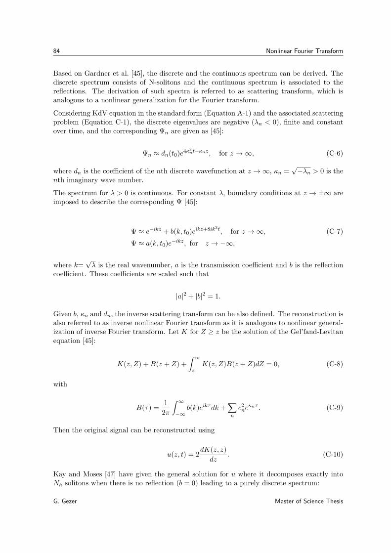
84 Nonlinear Fourier Transform
Based on Gardner et al. [45], the discrete and the continuous spectrum can be derived. Thediscrete spectrum consists of N-solitons and the continuous spectrum is associated to thereflections. The derivation of such spectra is referred to as scattering transform, which isanalogous to a nonlinear generalization for the Fourier transform.
Considering KdV equation in the standard form (Equation A-1) and the associated scatteringproblem (Equation C-1), the discrete eigenvalues are negative (λn < 0), finite and constantover time, and the corresponding Ψn are given as [45]:
Ψn ≈ dn(t0)e4κ3nt−κnz, for z →∞, (C-6)
where dn is the coefficient of the nth discrete wavefunction at z →∞, κn =√−λn > 0 is the
nth imaginary wave number.
The spectrum for λ > 0 is continuous. For constant λ, boundary conditions at z → ±∞ areimposed to describe the corresponding Ψ [45]:
Ψ ≈ e−ikz + b(k, t0)eikz+8ik3t, for z →∞, (C-7)Ψ ≈ a(k, t0)e−ikz, for z → −∞,
where k=√λ is the real wavenumber, a is the transmission coefficient and b is the reflection
coefficient. These coefficients are scaled such that
|a|2 + |b|2 = 1.
Given b, κn and dn, the inverse scattering transform can be also defined. The reconstruction isalso referred to as inverse nonlinear Fourier transform as it is analogous to nonlinear general-ization of inverse Fourier transform. Let K for Z ≥ z be the solution of the Gel’fand-Levitanequation [45]:
K(z, Z) +B(z + Z) +∫ ∞z
K(z, Z)B(z + Z)dZ = 0, (C-8)
with
B(τ) = 12π
∫ ∞−∞
b(k)eikτdk +∑n
c2neκnτ . (C-9)
Then the original signal can be reconstructed using
u(z, t) = 2dK(z, z)dz
. (C-10)
Kay and Moses [47] have given the general solution for u where it decomposes exactly intoNh solitons when there is no reflection (b = 0) leading to a purely discrete spectrum:
G. Gezer Master of Science Thesis

85
u(t) = 4~N∑n=1
κnΨ2n(t), (C-11)
where N is the number of discrete eigenvalues. Depending on the initial data and ~, N willbe finite and fixed.
Master of Science Thesis G. Gezer

86 Nonlinear Fourier Transform
G. Gezer Master of Science Thesis
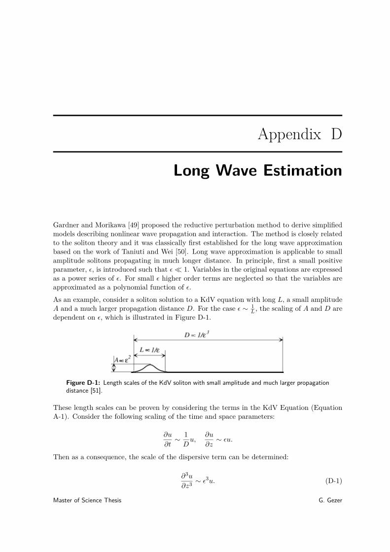
Appendix D
Long Wave Estimation
Gardner and Morikawa [49] proposed the reductive perturbation method to derive simplifiedmodels describing nonlinear wave propagation and interaction. The method is closely relatedto the soliton theory and it was classically first established for the long wave approximationbased on the work of Taniuti and Wei [50]. Long wave approximation is applicable to smallamplitude solitons propagating in much longer distance. In principle, first a small positiveparameter, ε, is introduced such that ε� 1. Variables in the original equations are expressedas a power series of ε. For small ε higher order terms are neglected so that the variables areapproximated as a polynomial function of ε.
As an example, consider a soliton solution to a KdV equation with long L, a small amplitudeA and a much larger propagation distance D. For the case ε ∼ 1
L , the scaling of A and D aredependent on ε, which is illustrated in Figure D-1.
Figure D-1: Length scales of the KdV soliton with small amplitude and much larger propagationdistance [51].
These length scales can be proven by considering the terms in the KdV Equation (EquationA-1). Consider the following scaling of the time and space parameters:
∂u
∂t∼ 1Du,
∂u
∂z∼ εu.
Then as a consequence, the scale of the dispersive term can be determined:
∂3u
∂z3 ∼ ε3u. (D-1)
Master of Science Thesis G. Gezer

88 Long Wave Estimation
For the KdV soliton the nonlinear term and the dispersive term has to compensate for eachother, so the scaling of these terms match each other which can be used to determine thescaling of u:
u∂u
∂z∼ εu2 = ε3u→ u ∼ ε2, (D-2)
which gives us the fundamental relationship, A ∝ ε2. Contribution of the time derivative andthe dispersive term can be set to equal each other to derive the scale of D with respect to ε:
∂u
∂t∼ 1Du = ε3u→ D ∝ ε−3. (D-3)
G. Gezer Master of Science Thesis
Bibliography
[1] M. Willemet, P. Chowienczyk, and J. Alastruey, “A database of virtual healthy subjectsto assess the accuracy of foot-to-foot pulse wave velocities for estimation of aortic stiff-ness,” American Journal of Physiology-Heart and Circulatory Physiology, vol. 309, no. 4,pp. H663–H675, 2015.
[2] F. Otto, “Die grundform des arteriellen pulses,” Zeitung fur Biologie, vol. 37, pp. 483–586, 1899.
[3] N. Westerhof, P. Sipkema, G. V. D. Bos, and G. Elzinga, “Forward and backward wavesin the arterial system,” Cardiovascular research, vol. 6, no. 6, pp. 648–656, 1972.
[4] Y. Hashizume, “Nonlinear pressure waves in a fluid-filled elastic tube,” Journal of thePhysical Society of Japan, vol. 54, no. 9, pp. 3305–3312, 1985.
[5] Y. Hashizume, “Nonlinear pressure wave propagation in arteries,” Journal of the PhysicalSociety of Japan, vol. 57, no. 12, pp. 4160–4168, 1988.
[6] S. Yomosa, “Solitary waves in large blood vessels,” Journal of the Physical society ofJapan, vol. 56, no. 2, pp. 506–520, 1987.
[7] E. Crépeau and M. Sorine, “Identifiability of a reduced model of pulsatile flow in anarterial compartment,” in Decision and Control, 2005 and 2005 European Control Con-ference. CDC-ECC’05. 44th IEEE Conference on, pp. 891–896, IEEE, 2005.
[8] H. Demiray, “Weakly nonlinear waves in a viscous fluid contained in a viscoelastic tubewith variable cross-section,” European Journal of Mechanics-A/Solids, vol. 24, no. 2,pp. 337–347, 2005.
[9] E. Crépeau and M. Sorine, “A reduced model of pulsatile flow in an arterial compart-ment,” Chaos, Solitons & Fractals, vol. 34, no. 2, pp. 594–605, 2007.
[10] A. Melis, Gaussian process emulators for 1D vascular models. PhD thesis, University ofSheffield, 2017.
Master of Science Thesis G. Gezer

90 Bibliography
[11] T.-M. Laleg, E. Crépeau, and M. Sorine, “Separation of arterial pressure into a nonlinearsuperposition of solitary waves and a windkessel flow,” Biomedical signal processing andcontrol, vol. 2, no. 3, pp. 163–170, 2007.
[12] T.-M. Laleg, E. Crépeau, Y. Papelier, and M. Sorine, “Arterial blood pressure analysisbased on scattering transform i,” in Engineering in Medicine and Biology Society, 2007.EMBS 2007. 29th Annual International Conference of the IEEE, pp. 5326–5329, IEEE,2007.
[13] T.-M. Laleg, C. Médigue, F. Cottin, and M. Sorine, “Arterial blood pressure analysisbased on scattering transform ii,” in Engineering in Medicine and Biology Society, 2007.EMBS 2007. 29th Annual International Conference of the IEEE, pp. 5330–5333, IEEE,2007.
[14] T.-M. Laleg-Kirati, C. Médigue, Y. Papelier, F. Cottin, and A. Van de Louw, “Validationof a semi-classical signal analysis method for stroke volume variation assessment: Acomparison with the PiCCO technique,” Annals of biomedical engineering, vol. 38, no. 12,pp. 3618–3629, 2010.
[15] T.-M. Laleg-Kirati, E. Crépeau, and M. Sorine, “Semi-classical signal analysis,” Mathe-matics of Control, Signals, and Systems, vol. 25, no. 1, pp. 37–61, 2013.
[16] Y. Mehta and D. Arora, “Newer methods of cardiac output monitoring,” World journalof cardiology, vol. 6, no. 9, p. 1022, 2014.
[17] J. X. Sun, A. T. Reisner, M. Saeed, T. Heldt, and R. G. Mark, “The cardiac output fromblood pressure algorithms trial,” Critical care medicine, vol. 37, no. 1, p. 72, 2009.
[18] A. J. Lee, J. H. Cohn, and J. S. Ranasinghe, “Cardiac output assessed by invasive andminimally invasive techniques,” Anesthesiology research and practice, vol. 2011, 2011.
[19] K. B. Domino, T. A. Bowdle, K. L. Posner, P. H. Spitellie, L. A. Lee, and F. W. Cheney,“Injuries and liability related to central vascular catheters: A closed claims analysis,”Anesthesiology: The Journal of the American Society of Anesthesiologists, vol. 100, no. 6,pp. 1411–1418, 2004.
[20] A. Katsikis, G. Karavolias, and V. Voudris, “Transfemoral percutaneous removal of aknotted swan-ganz catheter,” Catheterization and Cardiovascular Interventions, vol. 74,no. 5, pp. 802–804, 2009.
[21] M. M. Smith, D. W. Barbara, L. C. Torsher, and C. J. Jankowski, “Nonsurgical removalof knotted pulmonary artery catheter,” Journal of Medical Cases, vol. 4, no. 3, pp. 163–165, 2012.
[22] S. A. Esper and M. R. Pinsky, “Arterial waveform analysis,” Best Practice & ResearchClinical Anaesthesiology, vol. 28, no. 4, pp. 363–380, 2014.
[23] N. Westerhof, F. Bosman, C. J. De Vries, and A. Noordergraaf, “Analog studies of thehuman systemic arterial tree,” Journal of biomechanics, vol. 2, no. 2, pp. 121–143, 1969.
G. Gezer Master of Science Thesis

91
[24] L. Zanoli, S. Rastelli, G. Inserra, and P. Castellino, “Arterial structure and function ininflammatory bowel disease,” World Journal of Gastroenterology: WJG, vol. 21, no. 40,p. 11304, 2015.
[25] R. Burattini and G. Gnudi, “Computer identification of models for the arterial tree inputimpedance: comparison between two new simple models and first experimental results,”Medical and Biological Engineering and Computing, vol. 20, no. 2, pp. 134–144, 1982.
[26] L. Formaggia, D. Lamponi, and A. Quarteroni, “One-dimensional models for blood flowin arteries,” Journal of engineering mathematics, vol. 47, no. 3-4, pp. 251–276, 2003.
[27] H. Demiray, “Nonlinear waves in a viscous fluid contained in a viscoelastic tube,”Zeitschrift für angewandte Mathematik und Physik ZAMP, vol. 52, no. 6, pp. 899–912,2001.
[28] J. Misra and M. Patra, “A study of solitary waves in a tapered aorta by using the theoryof solitons,” Computers & Mathematics with Applications, vol. 54, no. 2, pp. 242–254,2007.
[29] J.-F. Paquerot and M. Remoissenet, “Dynamics of nonlinear blood pressure waves inlarge arteries,” Physics Letters A, vol. 194, no. 1-2, pp. 77–82, 1994.
[30] N. Westerhof, Physics of Heart and Circulation. CRC Press, 1993.
[31] C. G. Caro, T. Pedley, and R. Schroter, The mechanics of the circulation. CambridgeUniversity Press, 2012.
[32] C. G. Caro and R. M. Nerem, “Transport of 14c-4-cholesterol between serum and wall inthe perfused dog common carotid artery,” Circulation Research, vol. 32, no. 2, pp. 187–205, 1973.
[33] N. Smith, A. Pullan, and P. J. Hunter, “An anatomically based model of transientcoronary blood flow in the heart,” SIAM Journal on Applied mathematics, vol. 62, no. 3,pp. 990–1018, 2002.
[34] P. Hunter, Numerical simulation of arterial blood flow. PhD thesis, ResearchSpace@Auckland, 1972.
[35] G. Hagen, “Ueber die bewegung des wassers in engen cylindrischen röhren,” Annalen derPhysik, vol. 122, no. 3, pp. 423–442, 1839.
[36] J. L. Poiseuille, Recherches expérimentales sur le mouvement des liquides dans les tubesde très-petits diamètres. Imprimerie Royale, 1844.
[37] N. Xiao, J. Alastruey, and C. Alberto Figueroa, “A systematic comparison between1-D and 3-D hemodynamics in compliant arterial models,” International journal fornumerical methods in biomedical engineering, vol. 30, no. 2, pp. 204–231, 2014.
[38] A. Osborne and M. Petti, “Numerical inverse-scattering-transform analysis of laboratory-generated surface wave trains,” Physical Review E, vol. 47, no. 2, p. 1035, 1993.
Master of Science Thesis G. Gezer

92 Bibliography
[39] E. Boileau, P. Nithiarasu, P. J. Blanco, L. O. Müller, F. E. Fossan, L. R. Hellevik, W. P.Donders, W. Huberts, M. Willemet, and J. Alastruey, “A benchmark study of numericalschemes for one-dimensional arterial blood flow modelling,” International journal fornumerical methods in biomedical engineering, vol. 31, no. 10, p. e02732, 2015.
[40] X. Wang, J.-M. Fullana, and P.-Y. Lagrée, “Verification and comparison of four numericalschemes for a 1d viscoelastic blood flow model,” Computer methods in biomechanics andbiomedical engineering, vol. 18, no. 15, pp. 1704–1725, 2015.
[41] S. Sherwin, V. Franke, J. Peiró, and K. Parker, “One-dimensional modelling of a vascularnetwork in space-time variables,” Journal of Engineering Mathematics, vol. 47, no. 3-4,pp. 217–250, 2003.
[42] H. C. Chen, V. Patel, J. Wiek, S. M. Rassam, and E. M. Kohner, “Vessel diameterchanges during the cardiac cycle,” Eye, vol. 8, no. 1, p. 97, 1994.
[43] A. G. Brown, Y. Shi, A. Marzo, C. Staicu, I. Valverde, P. Beerbaum, P. V. Lawford,and D. R. Hose, “Accuracy vs. computational time: translating aortic simulations to theclinic,” Journal of biomechanics, vol. 45, no. 3, pp. 516–523, 2012.
[44] T. A. Driscoll, N. Hale, and L. N. Trefethen, “Chebfun guide,” 2014.
[45] C. S. Gardner, J. M. Greene, M. D. Kruskal, and R. M. Miura, “Method for solving theKorteweg-de Vries equation,” Physical review letters, vol. 19, no. 19, p. 1095, 1967.
[46] A. Osborne, “Nonlinear Fourier analysis for the infinite-interval Korteweg-de Vries equa-tion i: An algorithm for the direct scattering transform,” Journal of ComputationalPhysics, vol. 94, no. 2, pp. 284–313, 1991.
[47] I. Kay and H. Moses, “Reflectionless transmission through dielectrics and scatteringpotentials,” Journal of Applied Physics, vol. 27, no. 12, pp. 1503–1508, 1956.
[48] P. D. Lax, “Integrals of nonlinear equations of evolution and solitary waves,” Communi-cations on pure and applied mathematics, vol. 21, no. 5, pp. 467–490, 1968.
[49] C. Gardner and O. Morikawa, “Similarity in the asymptotic behaviour of collision-freehydromagnetic waves and water waves,” Sc. Rep. NYO, vol. 9082, 1960.
[50] T. Taniuti and C.-C. Wei, “Reductive perturbation method in nonlinear wave propaga-tion. i,” Journal of the Physical Society of Japan, vol. 24, no. 4, pp. 941–946, 1968.
[51] H. Leblond, “The reductive perturbation method and some of its applications,” Journalof Physics B: Atomic, Molecular and Optical Physics, vol. 41, no. 4, p. 043001, 2008.
G. Gezer Master of Science Thesis