Magnetostatic surface wave bright soliton propagation in ferrite-dielectric-metal structures

IEEE TRANSACTIONS ON MAGNETICS, VOL. 42, NO. 7, JULY 2006 1785

Magnetostatic Surface Wave Bright SolitonPropagation in Ferrite-Dielectric-Metal Structures

R. Marcelli1, S. A. Nikitov2, Yu. A. Filimonov3, A. A. Galishnikov3, A. V. Kozhevnikov3, and G. M. Dudko3

CNR-IMM, Rome Section, Microwave Microsystems Technology Group, 00133 Rome, ItalyInstitute of Radioengineering and Electronics RAS, Moscow 103907, Russia

Institute of Radioengineering and Electronics RAS, Saratov 410019, Russia

Magnetostatic surface wave (MSSW) bright solitons in a ferrite-dielectric-metal (FDM) structure have been studied experimentallyand numerically in the framework of the nonlinear Schrödinger equation. Attention was focused on the influence of the parametricinstability on the soliton formation and propagation. We also discussed the contribution of the nonsolitary (dispersive wave) part ofthe MSSW pulse on the soliton propagation, to show that their mutual interference leads to the leveling off or to the appearance ofsome peaks in the MSSW pulse output versus the input amplitude. We have also shown that for MSSW pulses with rectangular shape,the linear pulse compression caused by an induced phase modulation of the input pulse must be taken into account. Experiments wereperformed on FDM microstrip structures loaded by a 14-�m-thick yttrium iron garnet film, separated from the ground metal by an airgap with thickness h1 � 100 �m or h2 � 200 �m. It was found experimentally for MSSW with wavelength � � h that the modulationinstability leads to soliton formation for rectangular input pulses with duration � less than the characteristic transient time t� needed forthe onset of the parametric instability, while pulses with � � t� are mainly subjected to parametric instability. The measured thresholdamplitudes for parametric and modulation instabilities are in agreement with the theoretical predictions. An influence of additionalpumping in the form of both continuous-wave and pulsed signals on the soliton formation was studied. It was shown that an additionalpumping signal with duration � � t�, and amplitude above the threshold of the parametric instability, suppressed the MSSW soliton.Numerical modeling of the pulsewidth dependence on the microwave power during the propagation in the FDM structure yields resultsthat are in agreement with the experimental observations. Moreover, pulse narrowing due to the induced phase modulation of the inputpulse was numerically predicted. All of these effects are in agreement with the experimental findings.

Index Terms—Microwave devices, modulation instability, nonlinear microwave ferrites, solitons.

I. INTRODUCTION

MAGNETOSTATIC WAVE (MSW) pulse envelope soli-tons propagating in magnetic films have been studied for

many years as a promising kind of wave excitation for signalprocessing based on nonlinear microwave transmission lines[1]. Actually, by properly choosing the magnetic dc bias fielddirection, it is possible to excite the MSWs characterized by anonlinear dispersion relation (where is thefrequency, is the wave number, and is the MSW dimension-less complex amplitude), which fulfills the Lighthill criterionfor modulation instability [2]:

(1)

where and are the dispersion andnonlinear coefficients of the MSW, respectively. In high-qualityyttrium iron garnet (YIG) films, the threshold values of themicrowave incident powers needed for starting the modu-lation instability do not exceed 1 W. This can be observed inexperiments with films having thickness m and fer-romagnetic resonance (FMR) linewidth Oe. MSWscan be easily excited and detected by means of single microstripantennas at frequencies ranging from 1 to 20 GHz, typically.Finally, dispersion properties of MSWs can be modified bychanging the direction and the magnitude of the dc bias field,placing near the YIG film a surface metal screen, dielectric

Digital Object Identifier 10.1109/TMAG.2006.872005

or magnetic layers, as well as by resonance interaction withexchange or elastic modes of the ferrite structure.

As well established, three basic types of dipole MSWs insingle YIG films can be defined: forward volume (FVMSW),backward volume (BVMSW), and surface (MSSW) mag-netostatic waves. Both FVMSW and BVMSW are unstablefor soliton formation [2], while the dispersion law for dipoleMSSWs in ungrounded single YIG films does not allow thefulfillment of the Lighthill criterion (1). For that reason, duringthe last two decades, MSW pulse envelope bright solitons inYIG films have been intensively studied, namely by usinggeometries corresponding to FVMSW [3]–[6] and BVMSW[7]–[11]. On the other hand, due to the surface character, andthe consequent nonreciprocal and single-mode propagationregime, MSSWs are more appealing for device applications.

In [12], MSSW pulse propagation in a YIG film with surfacepinned spins was investigated. In those films, dipole MSSWscan be in phase synchronism with volume exchange modes [13].Resonance interaction of those waves can lead to an MSSW dis-persion relation which creates some narrow ( MHz) fre-quency bands at carrier frequencies lower than the resonanceone for the fulfillment of the Lighthill criterion. For this narrow-frequency band, the formation of pulse envelope bright soli-tons was observed [12]. However, simultaneously with changesin dispersion, MSSW losses gradually increase [14], thus ren-dering this effect difficult to be used for device applications[15].1

1It is worth noting that the hybridization with exchange volume waveschanges the character of the dipole MSSW, transforming it in a dipole-ex-change quasi-surface wave [16].

0018-9464/$20.00 © 2006 IEEE

1786 IEEE TRANSACTIONS ON MAGNETICS, VOL. 42, NO. 7, JULY 2006

Another possibility to change the MSSW dispersion for ob-taining the Lighthill criterion fulfilment is by using a metal plate,acting as an electrical ground, placed near the ferrite film sur-face and with an air gap (spacer) having a thickness betweenferrite and metal surfaces [17]. As the metal has an effective in-fluence only on the MSSW having wavelength comparablewith the gap thickness , one may expect significative changesof the MSSW dispersion characteristics at wavelengths .On the other hand, MSSWs with wavelengths have dis-persive characteristics corresponding to the isolated ferrite film.It is easy to understand that for MSSW wavelengths thedispersion curve has a change in the slope and, consequently,in the sign of the dispersion coefficient [17]. This “transient”part of the MSSW dispersion characteristic (labeled as “I” inthe following text and figures) corresponding to MSSW wave-lengths is suitable for soliton formation and self-mod-ulation effects [17], [18]. It is the aim of this paper to presentexperimental results concerning soliton formation and propaga-tion in FDM structures and to propose a numerical modelingof the MSSW pulse propagation on the basis of the nonlinearSchrödinger equation (NSE).

The modulation instability generated by four-magnon (4M)or second-order Suhl processes2 can be formally described byusing the conservation laws

(2)

where and are the wave-vector and the radian frequencycorresponding to the MSW excited in the YIG film, whileand are the values corresponding to the created nonequi-librium magnons. For the modulation instability development,in addition to criterion (1) it is needed that nonequilibriummagnons generated in processes (2) must be in phase withtraveling MSWs:

(3)

If the conditions (3) are not fulfilled ( , for ex-ample), we get an MSW parametric instability. One may ex-pect that in a real experiment both kinds of instabilities cancoexist, with mutual interactions between them. Moreover, bothof them can contribute to the reshaping of the MSW pulse enve-lope [3]–[11], [19] and a question arises on who is responsiblefor pulse shrinking or self-modulation in a real experiment. Onlya few papers are known where this question was discussed forcontinuous-wave (CW) [20] and pulse [21] regimes of the MSWexcitation. Here, our aim is to enter the details of this discussionon the basis of the MSSW propagation in an FDM structure.Such an analysis of the MSSWs in FDM configurations can bedivided in three parts, depending on the dispersion character-istic: (I), (II) and (III). For MSSWsat frequencies corresponding to branches II and III the criterion(1) is not valid because both the dispersive and the nonlinear

2The 4M processes for MSSW in YIG film dominates in the range of biasfields H > 2�M � 780 Oe, where three-magnon (3M) or first-order Suhlprocesses are prohibited by the conservation laws.

coefficient are negative and only the parametric in-stability is possible. In region I both modulation and parametricinstabilities can be developed. Those properties of the MSSWdispersion in an FDM structure give us a chance to compare thebehaviour of microwave pulse envelopes under the influence ofthe parametric instability only (regions II and III) and when bothkinds of instabilities are possible (region I).

Another question discussed here concerns with the problemof the soliton interaction with an additional MSSW signal prop-agating simultaneously with the soliton in the FDM structure.This problem has been recently considered for the soliton para-metric amplification [22]–[24] and control of soliton propaga-tion in a magnetic film [11], [25].

A possibility to realize a microwave control on the MSWmodulation instability development is given by the mechanismof the phase cross-modulation between two MSWs co-propa-gating in YIG films [25]–[28]. It was shown that an additionalMSW may lead to the suppression [25] or to the creation[26]–[28] of the conditions for modulation instability of theMSW propagating in the YIG film. Another mechanism canbe the influence of the parametric magnons, excited by anadditional MSW, on the MSW propagation [29].

Recently [11], the influence of additional CW MSW signalson the soliton propagation in YIG films was experimentallystudied for device geometries and dc magnetic bias conditionssuitable for the propagation of FVMSWs and BVMSWs. It wasshown that CW MSW signals at power levels above a well-de-fined threshold contributed to a strong damping of the soliton.As expected, both the pulse duration and the delay time betweenpulses (duty cycle) of the train used to excite the YIG delayline result in a strong influence on the pulse propagation. In thispaper, experimental results of the interaction between MSSWpulses in an FDM structure also will be presented.

In the most part of the literature dealing with experimentson MSW nonlinear propagation in YIG films, the reshaping ofthe microwave pulse envelope at the output transducer was fullytreated as a soliton. However, if the MSW input power exceedsthe threshold level for the soliton formation, part of the inputpulse energy is not “included” into the soliton and it contributesto form “nonsolitary” (dispersive) waves. The interference be-tween these waves may be responsible for leveling off the trendof the output peak versus the input amplitude of the MSSWpulse, which was previously reported also for FVMSW [4], [5]and BVMSW [7], [8]. It is worth noting that the dispersion hasan important contribution to the soliton formation and propaga-tion. First of all, the dispersion plays a feedback role in the de-velopment of the modulation instability and in the soliton for-mation. It is also well known that, due to the damping of theMSW pulse at a critical distance, it will become insufficient forsupporting a soliton and the pulse will become wider as it prop-agates longer. However, this is only a partial explanation. ForMSW pulses having an envelope close to a rectangular shape,one can expect a strong dispersive perturbation of the pulsefronts since the beginning of the propagation in the YIG film. Itwill be numerically predicted that the result of this process is thephase modulation of the flat part of the pulse (which was initiallywithout any modulation) contributing to the well-known pulsecompression effect in dispersive media. Experimental data of

MARCELLI et al.: MAGNETOSTATIC SURFACE WAVE BRIGHT SOLITON PROPAGATION IN FERRITE-DIELECTRIC-METAL STRUCTURES 1787

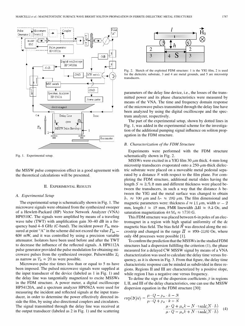
Fig. 1. Experimental setup.

the MSSW pulse compression effect in a good agreement withthe theoretical calculations will be presented.

II. EXPERIMENTAL RESULTS

A. Experimental Setup

The experimental setup is schematically shown in Fig. 1. Themicrowave signals were obtained from the synthesized sweeperof a Hewlett-Packard (HP) Vector Network Analyzer (VNA)HP8510C. The signals were amplified by means of a travelingwave tube (TWT) with amplification gain 30–40 dB in a fre-quency band 4–8 GHz (C-band). The incident power mea-sured at point “A” in the scheme did not exceed the value

mW, and it was controlled by using a precision variableattenuator. Isolators have been used before and after the TWTto decrease the influence of the reflected signals. A HP8112Apulse generator provided the pulse modulation for obtaining mi-crowave pulses from the synthesized sweeper. Pulsewidthsas narrow as ns were possible.

Microwave-pulse rise times less than or equal to 5 ns havebeen imposed. The pulsed microwave signals were supplied atthe input transducer of the device (labeled as 1 in Fig. 1) andthe delay line was tangentially magnetized to excite MSSWsin the FDM structure. A power meter, a digital oscilloscopeHP54120A, and a spectrum analyzer HP8562A were used formeasuring the incident and reflected signals at the input trans-ducer, in order to determine the power effectively directed in-side the film, by using also directional couplers and circulators.The signal transmitted through the delay line was received atthe output transducer (labeled as 2 in Fig. 1) and the scattering

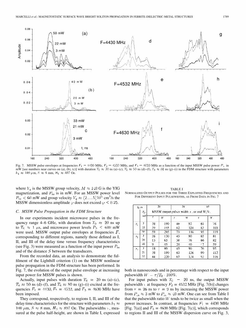
Fig. 2. Sketch of the exploited FDM structure: 1 is the YIG film, 2 is usedfor the dielectric substrate, 3 and 4 are metal grounds, and 5 are microstriptransducers.

parameters of the delay line device, i.e., the losses of the trans-mitted power and its phase characteristics were measured bymeans of the VNA. The time and frequency domain responseof the microwave pulses transmitted through the delay line havebeen analyzed by using the digital oscilloscope and the spec-trum analyzer, respectively.

The part of the experimental setup, shown by dotted lines inFig. 1, was added in the experimental scheme for the investiga-tion of the additional pumping signal influence on soliton prop-agation in the FDM structure.

B. Characterization of the FDM Structure

Experiments were performed with the FDM structureschematically shown in Fig. 2.

MSSWs were excited in a YIG film 30 m thick. 4-mm-longmicrostrip transducers evaporated onto a 250- m-thick dielec-tric substrate were placed on a moveable metal pedestal sepa-rated by a distance with respect to the film plane. For com-pleting the FDM structure, additional metal slides having thelength mm and different thickness were placed be-tween the transducers, in such a way that the distance be-tween the YIG and the metal surface was changed to obtain

m and m. The film dimensional andmagnetic parameters were: thickness m, widthmm, length mm, FMR linewidth Oe, andsaturation magnetization G.

This FDM structure was placed between 6-in poles of an elec-tromagnet in a region with high spatial uniformity of the dcmagnetic bias field. The bias field was directed along the mi-crostrip and changed in the range – Oe, whereonly 4M processes were possible [1].

To confirm the prediction that the MSSWs in the studied FDMstructures had a dispersion fulfilling the criterion (1), the phasemeasured for a delayed CW MSSW signal by means of a VNAcharacterization was used to calculate the delay time versus fre-quency, as it is shown in Fig. 3. From that figure, the delay timecharacteristic response can be minded as subdivided in three re-gions. Regions II and III are characterized by a positive slope,while region I has a negative one versus frequency.

To define the sign of the dispersion coefficients in regionsI, II, and III of the delay characteristics, one can use the MSSWdispersion equation in the FDM structure [30]:

(4)


Fig. 3. Experimental curves of the delay time versus frequency for the ex-ploited FDM structures, for two values (h � 100 �m and h � 200 �m)of the air spacer thickness. The separation between the input and output trans-ducers was S = 5 mm, and the dc bias field was H = 897 Oe.

Fig. 4. Calculated delay time (curve 1), dispersion (curve 2), nonlinear coef-ficient (curve 3) and wavenumbers (curve 4) versus frequency for the MSSWexcited in the exploited FDM structure, with parameters S = 5 mm, h =

200 �m, H = 987 Oe. Vertical and horizontal dotted lines indicate the fre-quency and wavenumbers interval corresponding to the region I of the delay linecharacteristics.

where

GHz/kOe is the gyro-magnetic ratio in YIG.The response of the MSSW-FDM device in terms of the delay

time, the coefficients for the dispersion and the nonlinearity, and the wavenumbers as a function of the frequency, cal-

culated from (4) for cm and other parame-ters as from Fig. 3, are shown in Fig. 4. For frequencies corre-sponding to region I the sign of the dispersion coefficient ispositive, while the nonlinearity coefficient is negative, as it isneeded for the soliton formation. It is worth noting that in theFDM structure used for our experiment the MSSW wavenum-bers belonging to region I of the dispersion characteristic arein the interval cm , as from curve 4 in Fig. 4.

To provide a microwave power level high enough for thedevelopment of the MSSW nonlinear processes, the insertionlosses of the delay line at different power levels for the input “A”of the experimental setup were preliminarily investigated—seeFig. 5.

Fig. 5. Experimental curves of the transmission losses versus frequency forthe exploited FDM structure, with parameters S = 5 mm, h � 200 �m fordifferent levels of the MW power at point “A” P —see Fig. 1. For curve 1the power at point “A” was in the range 6 < P < 20 mW. For curve 2:175 < P < 375 mW.

Fig. 6. MSSW power in the FDM structure with parameters correspondingto Fig. 4 versus the incident MW power P at point “A” of the experimentalscheme. The numbers refer to different frequencies: 1–4430 MHz, 2–4460 MHz,3–4500 MHz, 4–4530 MHz, 5–4600 MHz.

It was found that the transmission losses were unchanged formicrowave power levels less than 20 mW (point “A” in curve1 on Fig. 5). For higher powers the transmission losses are in-creased, as it is evidenced from the curve 2 in Fig. 5. An increaseof the transmission losses in the propagation of the MSSW in theFDM structure has been used in [29] to demonstrate the onsetof a nonlinear character for the surface wave. The MSSW inputpower , propagating in the FDM structure biased by the ex-ternal dc magnetic field , was calculated from the relation

(5)

where and are the power levels reflected fromthe input transducer and measured at dc bias fields in-band andout-of-band for the excitation of the surface waves. In Fig. 6,the MSSW input power calculated from (5) as a function of thepower available from the generator at point “A” for differentfrequencies is shown.

One can see that the MSSW power inside the film was in theorder of 10% with respect to the power level available atthe synthesizer. The dimensionless MSSW amplitude can beestimated from the following relation [29]:

(6)


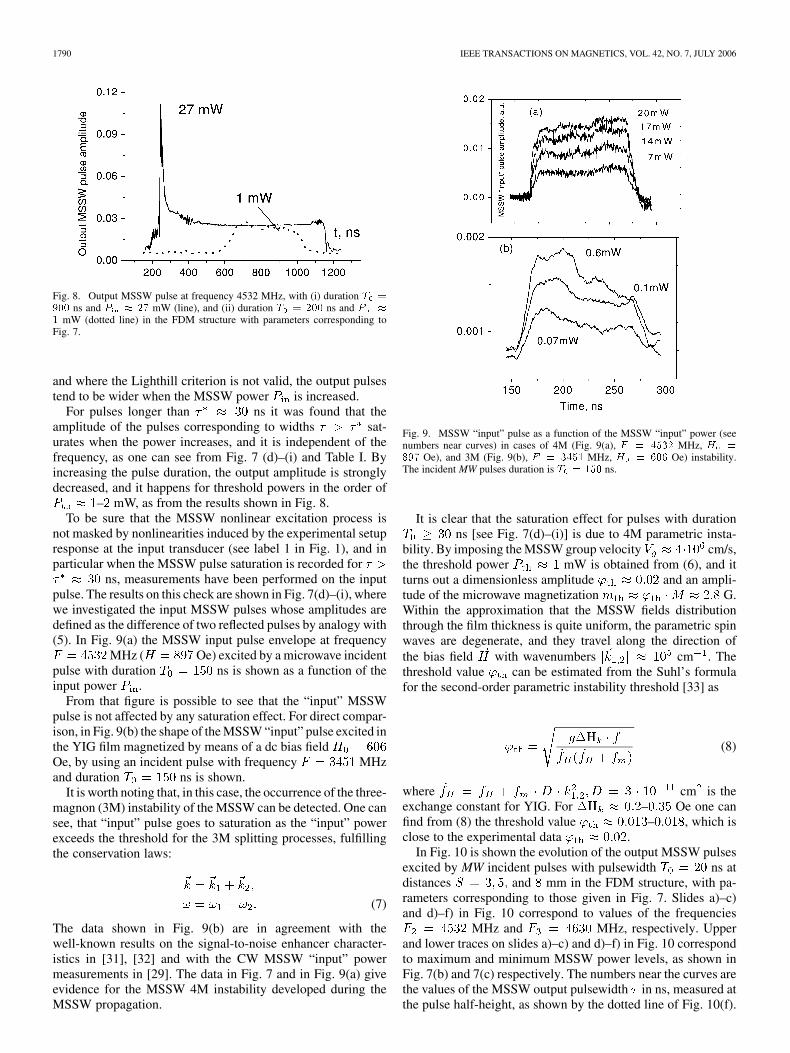
Fig. 7. MSSW pulse envelopes at frequencies F = 4430 MHz, F = 4532 MHz, and F = 4630 MHz as a function of the input MSSW pulse power P inmW [see numbers near curves on (a), (b), (c)] with duration T � 20 ns (a)–(c), T � 50 ns (d)–(f), T � 80 ns (g)–(i) in the FDM structure with parametersh � 100 �m, S � 8 mm, H � 897 Oe.

where is the MSSW group velocity, G is the YIGmagnetization, and is in mW. For an MSSW power level

mW and group velocity cm /s theMSSW dimensionless amplitude does not exceed .

C. MSSW Pulse Propagation in the FDM Structure

In our experiments incident microwave pulses in the fre-quency range 4–6 GHz, with duration from ns upto s, and microwave power levels mWwere used. MSSW output pulse envelopes at frequencies ,corresponding to different regions, namely those defined as I,II, and III of the delay time versus frequency characteristics(see Fig. 3) were measured as a function of the input powerand of the distance between the transducers.

From the recorded data, an analysis to demonstrate the ful-filment of the Lighthill criterion (1) on the MSSW nonlinearpulse propagation in the FDM structure has been performed. InFig. 7, the evolution of the output pulse envelope at increasinginput power for MSSW pulses is shown.

Actually, input pulses with duration ns (a)–(c),ns (d)–(f), and ns (g)–(i) excited at the fre-

quencies and MHz havebeen imposed.

They correspond, respectively, to regions I, II, and III of thedelay time characteristics for the structure with parameters

m, mm, Oe. The pulsewidths , mea-sured at the pulse half-height, are shown in Table I, expressed

TABLE INORMALIZED OUTPUT PULSES FOR THE THREE EXPLOITED FREQUENCIES AND

FOR DIFFERENT INPUT PULSEWIDTHS, AS FROM DATA IN FIG. 7

both in nanoseconds and in percentage with respect to the inputpulsewidth %.

For input pulses with ns, the output MSSWpulsewidth at frequency MHz [Fig. 7(b)] changesfrom ns to ns by increasing the MSSW powerfrom mW to mW. One can see from Table Ithat the pulsewidth ratio tends to be twice as small when thepower increases. In contrast, at frequencies MHz[Fig. 7(a)] and MHz [Fig. 7(c)], which correspondsto regions II and III of the MSSW dispersion curve on Fig. 3,


Fig. 8. Output MSSW pulse at frequency 4532 MHz, with (i) duration T =

900 ns and P � 27 mW (line), and (ii) duration T = 200 ns and P �

1 mW (dotted line) in the FDM structure with parameters corresponding toFig. 7.

and where the Lighthill criterion is not valid, the output pulsestend to be wider when the MSSW power is increased.

For pulses longer than ns it was found that theamplitude of the pulses corresponding to widths sat-urates when the power increases, and it is independent of thefrequency, as one can see from Fig. 7 (d)–(i) and Table I. Byincreasing the pulse duration, the output amplitude is stronglydecreased, and it happens for threshold powers in the order of

– mW, as from the results shown in Fig. 8.To be sure that the MSSW nonlinear excitation process is

not masked by nonlinearities induced by the experimental setupresponse at the input transducer (see label 1 in Fig. 1), and inparticular when the MSSW pulse saturation is recorded for

ns, measurements have been performed on the inputpulse. The results on this check are shown in Fig. 7(d)–(i), wherewe investigated the input MSSW pulses whose amplitudes aredefined as the difference of two reflected pulses by analogy with(5). In Fig. 9(a) the MSSW input pulse envelope at frequency

MHz ( Oe) excited by a microwave incidentpulse with duration ns is shown as a function of theinput power .

From that figure is possible to see that the “input” MSSWpulse is not affected by any saturation effect. For direct compar-ison, in Fig. 9(b) the shape of the MSSW “input” pulse excited inthe YIG film magnetized by means of a dc bias fieldOe, by using an incident pulse with frequency MHzand duration ns is shown.

It is worth noting that, in this case, the occurrence of the three-magnon (3M) instability of the MSSW can be detected. One cansee, that “input” pulse goes to saturation as the “input” powerexceeds the threshold for the 3M splitting processes, fulfillingthe conservation laws:

(7)

The data shown in Fig. 9(b) are in agreement with thewell-known results on the signal-to-noise enhancer character-istics in [31], [32] and with the CW MSSW “input” powermeasurements in [29]. The data in Fig. 7 and in Fig. 9(a) giveevidence for the MSSW 4M instability developed during theMSSW propagation.

Fig. 9. MSSW “input” pulse as a function of the MSSW “input” power (seenumbers near curves) in cases of 4M (Fig. 9(a), F = 4532 MHz, H =

897 Oe), and 3M (Fig. 9(b), F = 3451 MHz, H = 606 Oe) instability.The incident MW pulses duration is T = 150 ns.

It is clear that the saturation effect for pulses with durationns [see Fig. 7(d)–(i)] is due to 4M parametric insta-

bility. By imposing the MSSW group velocity cm/s,the threshold power mW is obtained from (6), and itturns out a dimensionless amplitude and an ampli-tude of the microwave magnetization G.Within the approximation that the MSSW fields distributionthrough the film thickness is quite uniform, the parametric spinwaves are degenerate, and they travel along the direction ofthe bias field with wavenumbers cm . Thethreshold value can be estimated from the Suhl’s formulafor the second-order parametric instability threshold [33] as

(8)

where cm is theexchange constant for YIG. For – Oe one canfind from (8) the threshold value – , which isclose to the experimental data .

In Fig. 10 is shown the evolution of the output MSSW pulsesexcited by MW incident pulses with pulsewidth ns atdistances and mm in the FDM structure, with pa-rameters corresponding to those given in Fig. 7. Slides a)–c)and d)–f) in Fig. 10 correspond to values of the frequencies

MHz and MHz, respectively. Upperand lower traces on slides a)–c) and d)–f) in Fig. 10 correspondto maximum and minimum MSSW power levels, as shown inFig. 7(b) and 7(c) respectively. The numbers near the curves arethe values of the MSSW output pulsewidth in ns, measured atthe pulse half-height, as shown by the dotted line of Fig. 10(f).


Fig. 10. MSSW output pulses as a function of the MSSW power at distancesS = 3 mm (a, d), S = 5 mm (b, e) and S = 8 mm (c, e) in an FDM struc-ture with parameters as in Fig. 7. Slides a)-c) and d)-f) correspond to MSSWpulses excited under experimental conditions equivalent to Fig. 7(b) and (c), re-spectively. Upper and lower traces on slides a)–c) and d)–f) correspond to max-imum and minimum MSSW power on Fig. 7(b) and (c), respectively. Numbersnear curves are the MSSW pulsewidth � in nanoseconds, measured at pulsehalf-height as shown by the dashed line on Fig. 10(f).

As expected, the role of nonlinearity in changing the pulse shapeis more and more pronounced when the distance increases.

At the frequency MHz, where the Lighthill crite-rion is fulfilled, the width of the MSSW pulses at the distance

mm were found ns and ns at MSSWpower mW and mW, respectively, as it isshown in Fig. 10(a). At distances mm and mmthe pulse shrinking is more evident by increasing the power, asit is shown in Fig. 10(b) and (c). For power values less than

mW the MSSW pulses are affected only by disper-sion broadening with increasing distance, as expected in linearregime [34].

The nonlinear broadening of the MSSW pulses with cen-tral frequency MHz increases with the distance ,as one can see from Fig. 10(d)–(f). However, at power levels

mW the MSSW pulsewidth is practically unchangedwith the distance, having the smallest width ns at thedistance mm, always a bit smaller than the incident MWpulsewidth ns. This result cannot be attributed to theaccuracy of the measurements and, as it is seen from Table I,was observed for the majority of the low-power MSSW pulses( mW), except for those output pulses corresponding toinput pulses with duration ns at frequencies and .These results are in contrast to expected linear pulse spreadingin dispersive media [34].

However, it will be discussed later that the pulse compressioncan really take place in linear dispersive regime at a critical dis-tance for input pulses with an almost rectangular envelopeshape.

In Fig. 11 are shown the results for the output peak amplitudeversus the input MSSW pulse amplitude obtained at

Fig. 11. MSSW output peak versus input pulse amplitude ' at frequenciesF ; F ; F and experimental conditions corresponding to Fig. 7(a)–(b). Thedashed lines indicate the linear dependence extrapolated from low amplitude.On Fig. 11(a) curves 1 and 2 represent ' (' ) at frequency F for a distancebetween the transducers S � 8 mm and S � 3 mm, respectively.

frequencies and experimental conditions corresponding to thosegiven in Fig. 7(a)–(b). In Fig. 11(a) the dependence forthe MSSW pulse with central frequency [as for Fig. 7(b)]obtained at distance mm is also shown in curve 2. Thedashed lines represent the linear behavior of the output signalwith increasing input amplitude.

As it is seen from Fig. 11(a), for amplitudes theMSSW output amplitude increases nonlinearly. This nonlinearincrease is consistent with the experimental results previouslyreported for MSFWV [4], [5] and MSBVW [7], [8]. The trendfor the curves has a similar behavior for both MSSWpropagation distances: mm (see curve 1) and mm(see curve 2). It is worth noting that the onset for an apparentleveling off or peak in the curves takes place at theMSSW input amplitudes – . From this we canargue that the existence of the peak in the curves couldnot be attributed only to the condition , i.e., to the bal-ance between the nonlinear length and the propagation one

, as it was discussed in [5]. In fact, the MSSW input amplitudescorresponding to the fulfillment of the condition at

distances mm and mm might be in the ratio(3 mm) / (8 mm) , while from our experimentwe find (3 mm) (8 mm), as it is shown in Fig. 11(a).It must be stressed that the excitation processes could not be re-sponsible for the onset of peaks in . This can be easilyseen from Figs. 6 and 9, where the MSSW power monotonouslyincreases with the incident MW power for both CW and pulseexcitation regime.

In our opinion, the nonlinear relaxation caused by parametricinstability has a small chance to be responsible for the onsetof peaks in , as it is shown in Fig. 11(a). Actually, atfrequencies and , where only the parametric instability


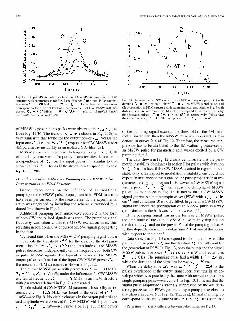
Fig. 12. Output MSSW pulse as a function of CW MSSW power in the FDMstructure with parameters as for Fig. 7 and distance S � 5 mm. Pulse parame-ters were F = 4400 MHz, T = 20 ns, P = 30 mW. Numbers near curvescorrespond to the different level of input power P of CW MSSW with fre-quency F = 4532 MHz: 1� P < P � 1 mW; 2–1.3 mW; 3–4 mW;4–10 mW; 5–21 mW; 6–27 mW.

of MSSW is possible, no peaks were observed in , asfrom Fig. 11(b). The trend of shown in Fig. 11(b) isvery similar to that found for the output power versus theinput one , i.e., the response for CW MSSW under4M parametric instability in an isolated YIG film [29].

MSSW pulses at frequencies belonging to regions I, II, IIIof the delay time versus frequency characteristics demonstratea dependence of on the input power similar to thatshown in Figs. 7–11 for an FDM structure with spacer thickness

m.

D. Influence of an Additional Pumping on the MSSW PulsePropagation in an FDM Structure

Further experiments on the influence of an additionalpumping on the MSSW pulse propagation in an FDM structurehave been performed. For the measurements, the experimentalsetup was upgraded by including the scheme surrounded by adotted line shown in Fig. 1.

Additional pumping from microwave source 2 in the formof both CW and pulsed signals was used. The pumping signalfrequency was taken within the MSSW excitation band, thusresulting in additional CW or pulsed MSSW signals propagatingin the film.

We found that when the MSSW CW pumping signal powerexceeds the threshold for the onset of the 4M para-

metric instability ( ) the amplitude of the MSSWpulses decreases, independently on the frequency, for both CWor pulse MSSW signals. The typical behavior of the MSSWoutput pulse as a function of the input CW MSSW power inthe measured FDM structures is shown in Fig. 12.

The output MSSW pulse with parameters MHz,ns, mW, under the influence of a CW MSSW

excited at frequency MHz in an FDM structurewith parameters defined in Fig. 7 is presented.

The threshold of CW MSSW 4M parametric instability at fre-quency MHz was found in the order of

mW—see Fig. 9. No visible changes in the output pulse shapeand amplitude were observed for CW MSSW with input power

mW—see curve 1 on Fig. 12. If the power

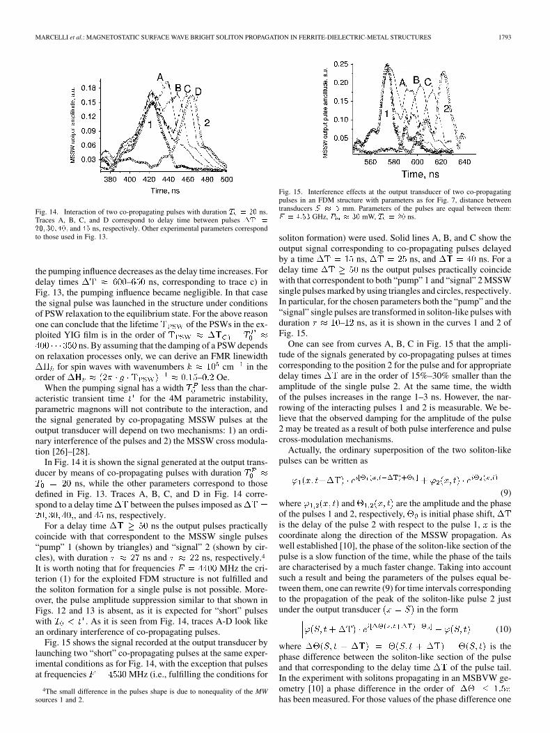
Fig. 13. Influence of a PSW excited by an MSSW pumping pulse: (1) withduration T = 250 ns on a “short” T = 20 ns MSSW signal pulse, and(2) propagation in FDM structure with parameters correspondent to Fig. 7 withdistance S � 5 mm. Traces a), b) and c) correspond to values of the delaytime between pulses �T = 250; 450; and 650 ns, respectively. Pulses havethe same frequency F = 4:4 GHz and power P � P � 30 mW.

of the pumping signal exceeds the threshold of the 4M para-metric instability, then the MSSW pulse is suppressed, as evi-denced in curves 2–6 of Fig. 12. Therefore, the measured sup-pression has to be attributed to the 4M scattering processes ofan MSSW pulse for parametric spin waves excited by a CWpumping signal.

The data shown in Fig. 12 clearly demonstrate that the para-metric instability dominates in region I for pulses with duration

ns. In fact, if the CW MSSW excited in region I is un-stable only with respect to modulation instability, one could notexpect an influence of this signal on the pulse propagation at fre-quencies belonging to region II. However, a CW MSSW signalwith a power will cause the damping of MSSWpulses, as evidenced in Fig. 12. It means that a CW MSSWsignal generates parametric spin waves (PSW) withcm , and condition (3) is not fulfilled. In general, a CW MSSWsignal influences the propagation of an MSSW pulse in a wayquite similar to the backward volume waves [11].

If the pumping signal was in the form of an MSSW pulse,the amplitude of the output MSSW pulse mainly depends onthe duration and on the power of the pumping pulse. Afurther dependence is on the delay time of one of the pulseswith respect to the other.3

Data shown in Fig. 13 correspond to the situation when thepumping pulse power and the duration are sufficient forthe generation of PSW. In Fig. 13, both the pump and the signalMSSW pulses have power mW and frequencies

GHz. The pumping pulse had a width ns,while the duration of the signal pulse was ns.

When the delay time was ns thepulses overlapped at the output transducer, resulting in an en-velope which was practically the same with respect to that for asingle pumping pulse—see curve 1 in Fig. 13. It means that thesignal pulse amplitude is strongly suppressed by the 4M scat-tering processes on PSWs generated by a pump pulse close tothat shown in curve 6 of Fig. 12. Traces a), b), and c) in Fig. 13correspond to the delay time values . It is seen that

3Delay time �T is time difference between pulses fronts; see Fig. 13.


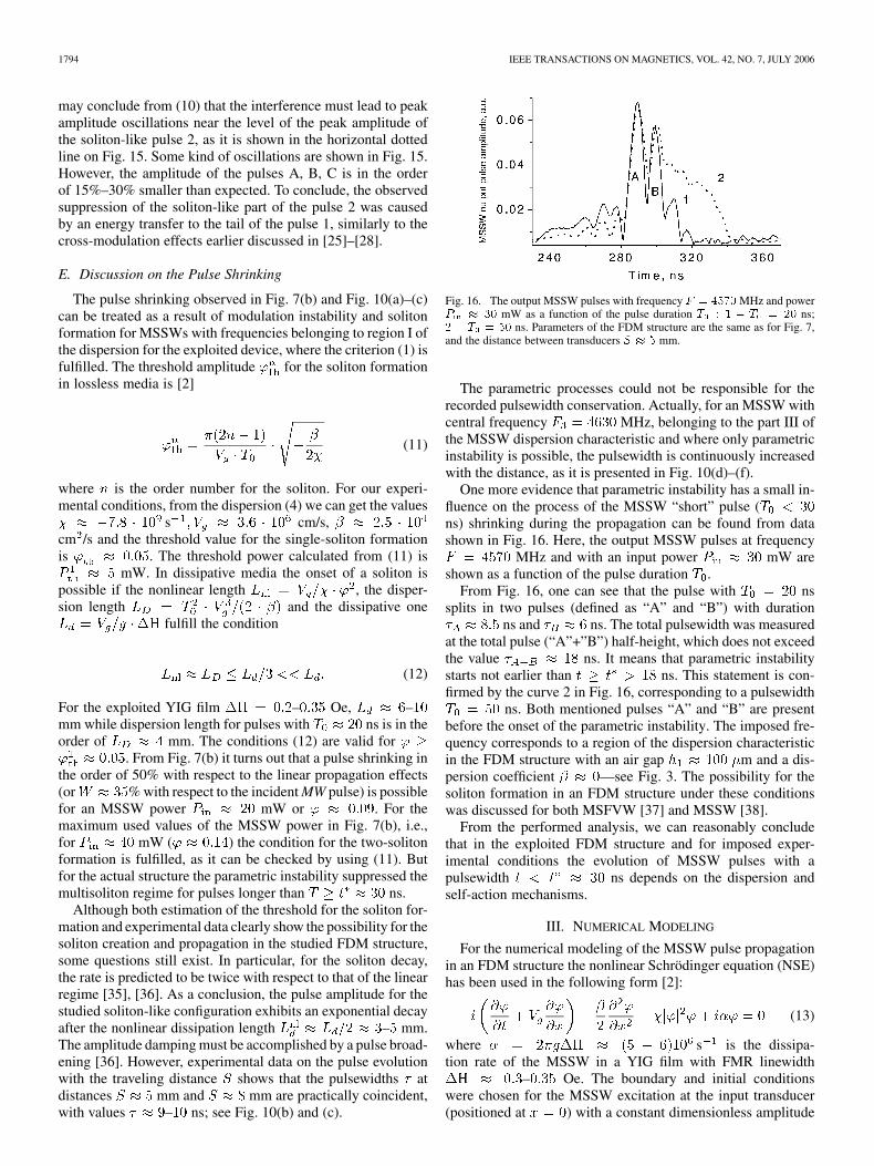
Fig. 14. Interaction of two co-propagating pulses with duration T = 20 ns.Traces A, B, C, and D correspond to delay time between pulses �T =

20; 30;40; and 45 ns, respectively. Other experimental parameters correspondto those used in Fig. 13.

the pumping influence decreases as the delay time increases. Fordelay times – ns, corresponding to trace c) inFig. 13, the pumping influence became negligible. In that casethe signal pulse was launched in the structure under conditionsof PSW relaxation to the equilibrium state. For the above reasonone can conclude that the lifetime of the PSWs in the ex-ploited YIG film is in the order of

ns. By assuming that the damping of a PSW dependson relaxation processes only, we can derive an FMR linewidth

for spin waves with wavenumbers cm in theorder of – Oe.

When the pumping signal has a width less than the char-acteristic transient time for the 4M parametric instability,parametric magnons will not contribute to the interaction, andthe signal generated by co-propagating MSSW pulses at theoutput transducer will depend on two mechanisms: 1) an ordi-nary interference of the pulses and 2) the MSSW cross modula-tion [26]–[28].

In Fig. 14 it is shown the signal generated at the output trans-ducer by means of co-propagating pulses with duration

ns, while the other parameters correspond to thosedefined in Fig. 13. Traces A, B, C, and D in Fig. 14 corre-spond to a delay time between the pulses imposed as

, and ns, respectively.For a delay time ns the output pulses practically

coincide with that correspondent to the MSSW single pulses“pump” 1 (shown by triangles) and “signal” 2 (shown by cir-cles), with duration ns and ns, respectively.4It is worth noting that for frequencies MHz the cri-terion (1) for the exploited FDM structure is not fulfilled andthe soliton formation for a single pulse is not possible. More-over, the pulse amplitude suppression similar to that shown inFigs. 12 and 13 is absent, as it is expected for “short” pulseswith . As it is seen from Fig. 14, traces A-D look likean ordinary interference of co-propagating pulses.

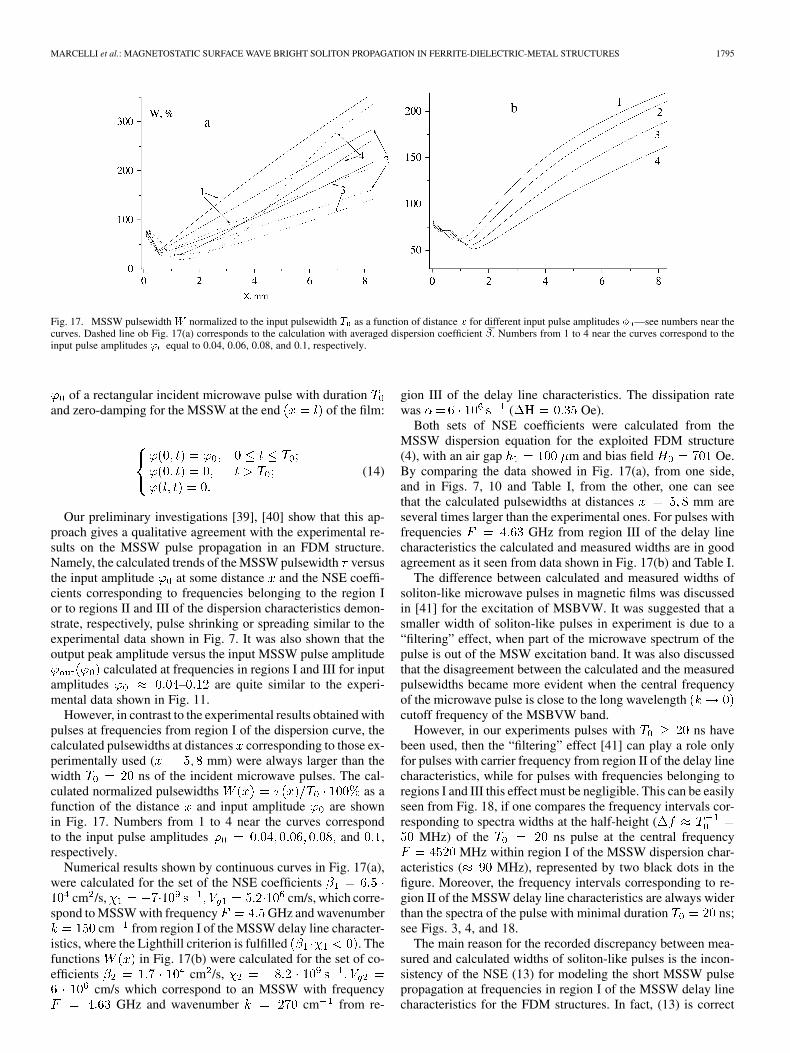
Fig. 15 shows the signal recorded at the output transducer bylaunching two “short” co-propagating pulses at the same exper-imental conditions as for Fig. 14, with the exception that pulsesat frequencies MHz (i.e., fulfilling the conditions for

4The small difference in the pulses shape is due to nonequality of the MWsources 1 and 2.

Fig. 15. Interference effects at the output transducer of two co-propagatingpulses in an FDM structure with parameters as for Fig. 7, distance betweentransducers S � 5 mm. Parameters of the pulses are equal between them:F = 4:53 GHz, P � 30 mW, T = 20 ns.

soliton formation) were used. Solid lines A, B, and C show theoutput signal corresponding to co-propagating pulses delayedby a time ns, ns, and ns. For adelay time ns the output pulses practically coincidewith that correspondent to both “pump” 1 and “signal” 2 MSSWsingle pulses marked by using triangles and circles, respectively.In particular, for the chosen parameters both the “pump” and the“signal” single pulses are transformed in soliton-like pulses withduration – ns, as it is shown in the curves 1 and 2 ofFig. 15.

One can see from curves A, B, C in Fig. 15 that the ampli-tude of the signals generated by co-propagating pulses at timescorresponding to the position 2 for the pulse and for appropriatedelay times are in the order of 15%–30% smaller than theamplitude of the single pulse 2. At the same time, the widthof the pulses increases in the range 1–3 ns. However, the nar-rowing of the interacting pulses 1 and 2 is measurable. We be-lieve that the observed damping for the amplitude of the pulse2 may be treated as a result of both pulse interference and pulsecross-modulation mechanisms.

Actually, the ordinary superposition of the two soliton-likepulses can be written as

(9)where and are the amplitude and the phaseof the pulses 1 and 2, respectively, is initial phase shift,is the delay of the pulse 2 with respect to the pulse 1, is thecoordinate along the direction of the MSSW propagation. Aswell established [10], the phase of the soliton-like section of thepulse is a slow function of the time, while the phase of the tailsare characterised by a much faster change. Taking into accountsuch a result and being the parameters of the pulses equal be-tween them, one can rewrite (9) for time intervals correspondingto the propagation of the peak of the soliton-like pulse 2 justunder the output transducer in the form

(10)

where is thephase difference between the soliton-like section of the pulseand that corresponding to the delay time of the pulse tail.In the experiment with solitons propagating in an MSBVW ge-ometry [10] a phase difference in the order ofhas been measured. For those values of the phase difference one


may conclude from (10) that the interference must lead to peakamplitude oscillations near the level of the peak amplitude ofthe soliton-like pulse 2, as it is shown in the horizontal dottedline on Fig. 15. Some kind of oscillations are shown in Fig. 15.However, the amplitude of the pulses A, B, C is in the orderof 15%–30% smaller than expected. To conclude, the observedsuppression of the soliton-like part of the pulse 2 was causedby an energy transfer to the tail of the pulse 1, similarly to thecross-modulation effects earlier discussed in [25]–[28].

E. Discussion on the Pulse Shrinking

The pulse shrinking observed in Fig. 7(b) and Fig. 10(a)–(c)can be treated as a result of modulation instability and solitonformation for MSSWs with frequencies belonging to region I ofthe dispersion for the exploited device, where the criterion (1) isfulfilled. The threshold amplitude for the soliton formationin lossless media is [2]

(11)

where is the order number for the soliton. For our experi-mental conditions, from the dispersion (4) we can get the values

s cm/s,cm /s and the threshold value for the single-soliton formationis . The threshold power calculated from (11) is

mW. In dissipative media the onset of a soliton ispossible if the nonlinear length , the disper-sion length and the dissipative one

fulfill the condition

(12)

For the exploited YIG film – Oe, –mm while dispersion length for pulses with ns is in theorder of mm. The conditions (12) are valid for

. From Fig. 7(b) it turns out that a pulse shrinking inthe order of 50% with respect to the linear propagation effects(or % with respect to the incident MW pulse) is possiblefor an MSSW power mW or . For themaximum used values of the MSSW power in Fig. 7(b), i.e.,for mW ( ) the condition for the two-solitonformation is fulfilled, as it can be checked by using (11). Butfor the actual structure the parametric instability suppressed themultisoliton regime for pulses longer than ns.

Although both estimation of the threshold for the soliton for-mation and experimental data clearly show the possibility for thesoliton creation and propagation in the studied FDM structure,some questions still exist. In particular, for the soliton decay,the rate is predicted to be twice with respect to that of the linearregime [35], [36]. As a conclusion, the pulse amplitude for thestudied soliton-like configuration exhibits an exponential decayafter the nonlinear dissipation length – mm.The amplitude damping must be accomplished by a pulse broad-ening [36]. However, experimental data on the pulse evolutionwith the traveling distance shows that the pulsewidths atdistances mm and mm are practically coincident,with values – ns; see Fig. 10(b) and (c).

Fig. 16. The output MSSW pulses with frequency F = 4570 MHz and powerP � 30 mW as a function of the pulse duration T : 1 � T = 20 ns;2 � T = 50 ns. Parameters of the FDM structure are the same as for Fig. 7,and the distance between transducers S � 5 mm.

The parametric processes could not be responsible for therecorded pulsewidth conservation. Actually, for an MSSW withcentral frequency MHz, belonging to the part III ofthe MSSW dispersion characteristic and where only parametricinstability is possible, the pulsewidth is continuously increasedwith the distance, as it is presented in Fig. 10(d)–(f).

One more evidence that parametric instability has a small in-fluence on the process of the MSSW “short” pulse (ns) shrinking during the propagation can be found from datashown in Fig. 16. Here, the output MSSW pulses at frequency

MHz and with an input power mW areshown as a function of the pulse duration .

From Fig. 16, one can see that the pulse with nssplits in two pulses (defined as “A” and “B”) with duration

ns and ns. The total pulsewidth was measuredat the total pulse (“A”+”B”) half-height, which does not exceedthe value ns. It means that parametric instabilitystarts not earlier than ns. This statement is con-firmed by the curve 2 in Fig. 16, corresponding to a pulsewidth

ns. Both mentioned pulses “A” and “B” are presentbefore the onset of the parametric instability. The imposed fre-quency corresponds to a region of the dispersion characteristicin the FDM structure with an air gap m and a dis-persion coefficient —see Fig. 3. The possibility for thesoliton formation in an FDM structure under these conditionswas discussed for both MSFVW [37] and MSSW [38].

From the performed analysis, we can reasonably concludethat in the exploited FDM structure and for imposed exper-imental conditions the evolution of MSSW pulses with apulsewidth ns depends on the dispersion andself-action mechanisms.

III. NUMERICAL MODELING

For the numerical modeling of the MSSW pulse propagationin an FDM structure the nonlinear Schrödinger equation (NSE)has been used in the following form [2]:

(13)

where s is the dissipa-tion rate of the MSSW in a YIG film with FMR linewidth

– Oe. The boundary and initial conditionswere chosen for the MSSW excitation at the input transducer(positioned at ) with a constant dimensionless amplitude


Fig. 17. MSSW pulsewidth W normalized to the input pulsewidth T as a function of distance x for different input pulse amplitudes � —see numbers near thecurves. Dashed line ob Fig. 17(a) corresponds to the calculation with averaged dispersion coefficient ��. Numbers from 1 to 4 near the curves correspond to theinput pulse amplitudes ' equal to 0.04, 0.06, 0.08, and 0.1, respectively.

of a rectangular incident microwave pulse with durationand zero-damping for the MSSW at the end of the film:

(14)

Our preliminary investigations [39], [40] show that this ap-proach gives a qualitative agreement with the experimental re-sults on the MSSW pulse propagation in an FDM structure.Namely, the calculated trends of the MSSW pulsewidth versusthe input amplitude at some distance and the NSE coeffi-cients corresponding to frequencies belonging to the region Ior to regions II and III of the dispersion characteristics demon-strate, respectively, pulse shrinking or spreading similar to theexperimental data shown in Fig. 7. It was also shown that theoutput peak amplitude versus the input MSSW pulse amplitude

calculated at frequencies in regions I and III for inputamplitudes – are quite similar to the experi-mental data shown in Fig. 11.

However, in contrast to the experimental results obtained withpulses at frequencies from region I of the dispersion curve, thecalculated pulsewidths at distances corresponding to those ex-perimentally used ( mm) were always larger than thewidth ns of the incident microwave pulses. The cal-culated normalized pulsewidths as afunction of the distance and input amplitude are shownin Fig. 17. Numbers from 1 to 4 near the curves correspondto the input pulse amplitudes and ,respectively.

Numerical results shown by continuous curves in Fig. 17(a),were calculated for the set of the NSE coefficients

cm /s, cm/s, which corre-spond to MSSW with frequency GHz and wavenumber

cm from region I of the MSSW delay line character-istics, where the Lighthill criterion is fulfilled . Thefunctions in Fig. 17(b) were calculated for the set of co-efficients cm /s,

cm/s which correspond to an MSSW with frequencyGHz and wavenumber cm from re-

gion III of the delay line characteristics. The dissipation ratewas ( Oe).

Both sets of NSE coefficients were calculated from theMSSW dispersion equation for the exploited FDM structure(4), with an air gap m and bias field Oe.By comparing the data showed in Fig. 17(a), from one side,and in Figs. 7, 10 and Table I, from the other, one can seethat the calculated pulsewidths at distances mm areseveral times larger than the experimental ones. For pulses withfrequencies GHz from region III of the delay linecharacteristics the calculated and measured widths are in goodagreement as it seen from data shown in Fig. 17(b) and Table I.

The difference between calculated and measured widths ofsoliton-like microwave pulses in magnetic films was discussedin [41] for the excitation of MSBVW. It was suggested that asmaller width of soliton-like pulses in experiment is due to a“filtering” effect, when part of the microwave spectrum of thepulse is out of the MSW excitation band. It was also discussedthat the disagreement between the calculated and the measuredpulsewidths became more evident when the central frequencyof the microwave pulse is close to the long wavelengthcutoff frequency of the MSBVW band.

However, in our experiments pulses with ns havebeen used, then the “filtering” effect [41] can play a role onlyfor pulses with carrier frequency from region II of the delay linecharacteristics, while for pulses with frequencies belonging toregions I and III this effect must be negligible. This can be easilyseen from Fig. 18, if one compares the frequency intervals cor-responding to spectra widths at the half-height (

MHz) of the ns pulse at the central frequencyMHz within region I of the MSSW dispersion char-

acteristics ( MHz), represented by two black dots in thefigure. Moreover, the frequency intervals corresponding to re-gion II of the MSSW delay line characteristics are always widerthan the spectra of the pulse with minimal duration ns;see Figs. 3, 4, and 18.

The main reason for the recorded discrepancy between mea-sured and calculated widths of soliton-like pulses is the incon-sistency of the NSE (13) for modeling the short MSSW pulsepropagation at frequencies in region I of the MSSW delay linecharacteristics for the FDM structures. In fact, (13) is correct


Fig. 18. MSSW delay time characteristics in the exploited FDM structure (A),MSSW pulse spectra at the central frequency F = 4520 MHz and pulsewidthT = 20 ns (B) and wavenumbers k versus Frequency (C). Two black dotsindicate the boundaries of the dispersion region I of the MSSW dispersion char-acteristic, where the Lighthill criterion is fulfilled. The �f marks the width ofthe MSSW pulse spectra at the pulse half-height (�3 dB). The horizontal dottedlines indicate the wavenumbers interval corresponding to the region I.

for both temporal and spatial spectral narrow wave packets ful-filling the following equations:

(15a)

(15b)

It is also expected that the NSE coefficients do notchange across the wave packet width and, consequently, theLighthill criterion (1) must be fulfilled for all the spectral com-ponents of the pulse.

From Figs. 18 and 4, one can see that in the exploitedFDM structures the dispersion coefficient gradually changesthrough the spectral width MHz of the MSSW pulseswith duration ns and central frequencies belonging tothe region I of the MSSW delay line characteristics, where thecriterion (1) is fulfilled. In this case an adequate approach fornumerical modeling of soliton propagation must be based on thesystem of coupled NSE [42], [43], [26]–[28], where the numberof the equations corresponds to the number of harmonics of thepulse spectra. However, in this paper we will use a simplifiedapproach, based on a NSE with weighted spectral components,by using the pulse spectra dispersion coefficient . As a matterof fact, a good agreement is obtained with experimental results.

A. Calculation Results Based on NSE With WeightedDispersion Coefficient

The weight for the pulse spectra components leads to the fol-lowing definition of the dispersion coefficient :

(16)

where and are the bound-aries of the frequency interval corresponding to the pulse spectrawidth at the pulse (spectral function ) half-height. Fromdata shown in Figs. 4 and 18 one can expect, that averagedvalues for pulses with central frequencies from regions I

Fig. 19. Envelope MSSW pulses j'(x ; t)j calculated at the distances x =3 mm, x = 5 mm, and x = 8 mm as a function of the input amplitude. Thecurves in Fig. 19(a) and (b) were calculated for the same parameters used forW (x) shown in Fig. 17(a) by solid and dashed curves, respectively. The pulsesshown in Fig. 19(c) were calculated for parameters corresponding to Fig. 17(b).Numbers from 1 to 4 near the curves correspond to an input pulse amplitude' = 0:04;0:06; 0:08; and 0:1, respectively. The pulsewidths were foundpractically unchanged for input amplitudes ' smaller than the threshold value' .

and II of the delay line characteristics could be several timessmaller or change sign with respect to the dispersion coefficient

calculated in the usual way at the frequency from (4). Asan example, for the parameters of the MSSW pulse and FDMstructure in Fig. 18, the coefficients are cm /sand cm /s.

The influence of the approach based on the average of thedispersion coefficient on the results of the numerically solved(13) and (14) is shown by dotted lines in Figs. 17(a) and 19(b).

In Fig. 17(a), the normalized pulsewidths calculatedfrom NSE with weighted dispersion coefficients are plottedby using a dashed line. It is evidenced that the calculatedpulsewidths for input amplitudes is closer to theexperimental values, as from the dotted line in Fig. 17(a) andTable I. However, the curve for has a quite different


character with respect to the experimental results. The pos-sible origin of this discrepancy will be discussed in the nextparagraph.

In Fig. 19, the envelope MSSW pulses calculatedat the distances mm, mm, and mmas a function of the input amplitude are shown. The curves inFig. 19(a) and (b) were calculated for the same parameters usedfor shown in Fig. 17(a) by solid and dashed curves, re-spectively. The pulses shown in Fig. 19(c) were calculated forparameters corresponding to Fig. 17(b). Numbers from 1 to 4near curves correspond to the input pulse amplitudes equalto 0.04, 0.06, 0.08, and 0.1, respectively. The pulsewidths werefound practically unchanged for input amplitudes smallerthan the threshold value . The threshold value for the inputamplitude obtained from numerical solutions of the NSE withan ordinary dispersion coefficient cm /s wascalculated as , while by using the weighted disper-sion coefficient cm /s measurable changes inthe calculated pulses occurs for . The valuesfor calculated from (13) and (14) coincide with those ob-tained by using the formula (11) and they are quite close to theexperimental ones. It is seen from Fig. 19(a) and (b) that for pa-rameters of NSE equation which allow for the soliton formationthe pulses tend to be narrower by increasing the power. How-ever, pulse shrinking was obtained only for input amplitudes inthe range . For input amplitudes ,the pulse amplitude starts to decrease while the width increases.For higher values of the dispersion coefficient, a larger propa-gation distance is needed to observe the saturation of the outputpulse amplitude. The leveling off in the experimental findingsfor was also observed, as it is shown in Fig. 11(a). Bycomparing the pulsewidths in Fig. 19(b) and Fig. 19(a), one cansee that data calculated with weighted dispersion coefficientsare in good agreement with the experimental ones.

Calculated pulses for NSE solutions corresponding to regionIII of the delay line characteristics are affected only pulse broad-ening, as shown in Fig. 19(c). Numerical results calculated forboth weighted and ordinary dispersion coefficients demonstratea good fit to experimental data; actually the calculated and ex-perimental pulses are practically coincident. This is justified bythe fact that the values and practically coincide for pulsesfrom region III of the delay line characteristics (except of thefrequency interval close to region I).

B. Soliton and Nonsolitary Part (Dispersive Wave)Interaction Effects

As well established [44], [45], in the lossless approximationthe solitonic solutions of NSE involve damping oscillations be-fore reaching the stationary amplitude. This happens for pulseswith initial shape different from the hyperbolic-secant solutionsas well as for pulses with initial shape and ampli-tude within the range , where isthe threshold of the input amplitude for -soliton formation.This damping oscillations are due to the superposition of soli-tonic and nonsolitonic contributions in the pulse, where the non-solitonic part decreases during the propagation because of thedispersion spreading. An apparent leveling off or peak in the

trend for soliton-like pulses in Fig. 11(a) as well as adecrease of the peak pulse amplitude for in Fig. 19

Fig. 20. The pulses energy j'(x)j calculated from (13) and (14) in the losslessapproximation at fixed times for input amplitude values corresponding to ' =' = 0:01 (a), ' = ' = 0:03 (b), and ' < ' = 0:026 < ' (c).

can be observed as a result of the interference of the co-prop-agating soliton-like and nonsolitary (dispersive wave) parts ofthe MSSW pulse along the same trajectory.

In Fig. 20, the pulses amplitude distribution alongthe magnetic film calculated from (13), (14) in the lossless

approximation and for other NSE coefficients asfor Fig. 17 is shown as a function of . Input amplitudesfor calculated traces a), b), and c) in Fig. 20 were taken as

and ,respectively. The values for the input amplitudes andcorrespond to thresholds of single- and two-soliton formationdefined by (11). It is seen that for input amplitudes andthe behavior of the numerical solutions of the NSE (13) withinitial and boundary conditions (14) is very close to single- andtwo-soliton regimes, as one can expect from (11). However, forpulses with an input amplitude the shape changes as it


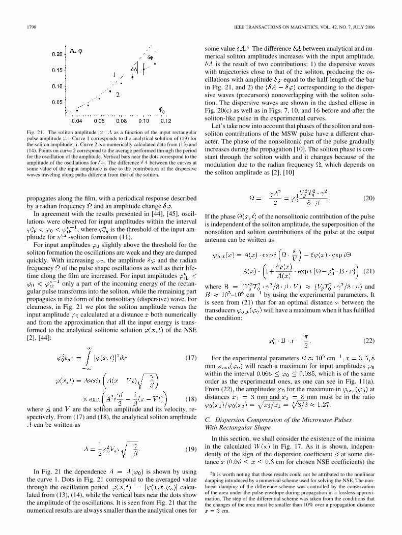
Fig. 21. The soliton amplitude j'j; A as a function of the input rectangularpulse amplitude ' . Curve 1 corresponds to the analytical solution of (19) forthe soliton amplitude A. Curve 2 is a numerically calculated data from (13) and(14). Points on curve 2 correspond to the average performed through the periodfor the oscillation of the amplitude. Vertical bars near the dots correspond to theamplitude of the oscillations for �'. The difference �A between the curves atsome value of the input amplitude is due to the contribution of the dispersivewaves traveling along paths different from that of the soliton.

propagates along the film, with a periodical response describedby a radian frequency and an amplitude change .

In agreement with the results presented in [44], [45], oscil-lations were observed for input amplitudes within the interval

, where is the threshold of the input am-plitude for -soliton formation (11).

For input amplitudes slightly above the threshold for thesoliton formation the oscillations are weak and they are dampedquickly. With increasing , the amplitude and the radianfrequency of the pulse shape oscillations as well as their life-time along the film are increased. For input amplitudes

only a part of the incoming energy of the rectan-gular pulse transforms into the soliton, while the remaining partpropagates in the form of the nonsolitary (dispersive) wave. Forclearness, in Fig. 21 we plot the soliton amplitude versus theinput amplitude calculated at a distance both numericallyand from the approximation that all the input energy is trans-formed to the analytical solitonic solution of the NSE[2], [44]:

(17)

(18)

where and are the soliton amplitude and its velocity, re-spectively. From (17) and (18), the analytical soliton amplitude

can be written as

(19)

In Fig. 21 the dependence is shown by usingthe curve 1. Dots in Fig. 21 correspond to the averaged valuethrough the oscillation period calcu-lated from (13), (14), while the vertical bars near the dots showthe amplitude of the oscillations. It is seen from Fig. 21 that thenumerical results are always smaller than the analytical ones for

some value .5 The difference between analytical and nu-merical soliton amplitudes increases with the input amplitude.

is the result of two contributions: 1) the dispersive waveswith trajectories close to that of the soliton, producing the os-cillations with amplitude equal to the half-length of the barin Fig. 21, and 2) the corresponding to the disper-sive waves (precursors) nonoverlapping with the soliton solu-tion. The dispersive waves are shown in the dashed ellipse inFig. 20(c) as well as in Figs. 7, 10, and 16 before and after thesoliton-like pulse in the experimental curves.

Let’s take now into account that phases of the soliton and non-soliton contributions of the MSW pulse have a different char-acter. The phase of the nonsolitonic part of the pulse graduallyincreases during the propagation [10]. The soliton phase is con-stant through the soliton width and it changes because of themodulation due to the radian frequency , which depends onthe soliton amplitude as [2], [10]

(20)

If the phase of the nonsolitonic contribution of the pulseis independent of the soliton amplitude, the superposition of thenonsoliton and soliton contributions of the pulse at the outputantenna can be written as

(21)

where and– cm by using the experimental parameters. It

is seen from (21) that for an optimal distance between thetransducers will have a maximum when it has fulfilledthe condition:

(22)

For the experimental parameters cmmm will reach a maximum for input amplitudeswithin the interval , which is of the sameorder as the experimental ones, as one can see in Fig. 11(a).From (22), the amplitudes for the maximum in atdistances mm and mm must be in the ratio

.

C. Dispersion Compression of the Microwave PulsesWith Rectangular Shape

In this section, we shall consider the existence of the minimain the calculated in Fig. 17. As it is shown, indepen-dently of the sign of the dispersion coefficient at some dis-tance ( cm for chosen NSE coefficients) the

5It is worth noting that these results could not be attributed to the nonlineardamping introduced by a numerical scheme used for solving the NSE. The non-linear damping of the difference scheme was controlled by the conservationof the area under the pulse envelope during propagation in a lossless approxi-mation. The step of the differential scheme was taken from the conditions thatthe changes of the area must be smaller than 10% over a propagation distancex = 3 cm.


Fig. 22. Envelope j'(x; t)j (full line) and phase �(x; t) (dotted line) of theMSSW pulse calculated from (13) with initial and boundary conditions (14)in a linear (� = 0) and lossless (� = 0) medium. Parameters in (13) wereV = 3:6 � 10 cm/s; � = �10 cm /s, T = 20 ns.

MSSW pulsewidth at the half-height calculated for input am-plitudes less than the threshold necessary for the onsetof the self-action mechanisms is smaller than thewidth of the incident MW pulse . It is worth notingthat the position for the minima of are sensitive to thedispersion coefficient values, as it is seen from comparison ofdata in Fig. 17(a), corresponding to the dispersion coefficients

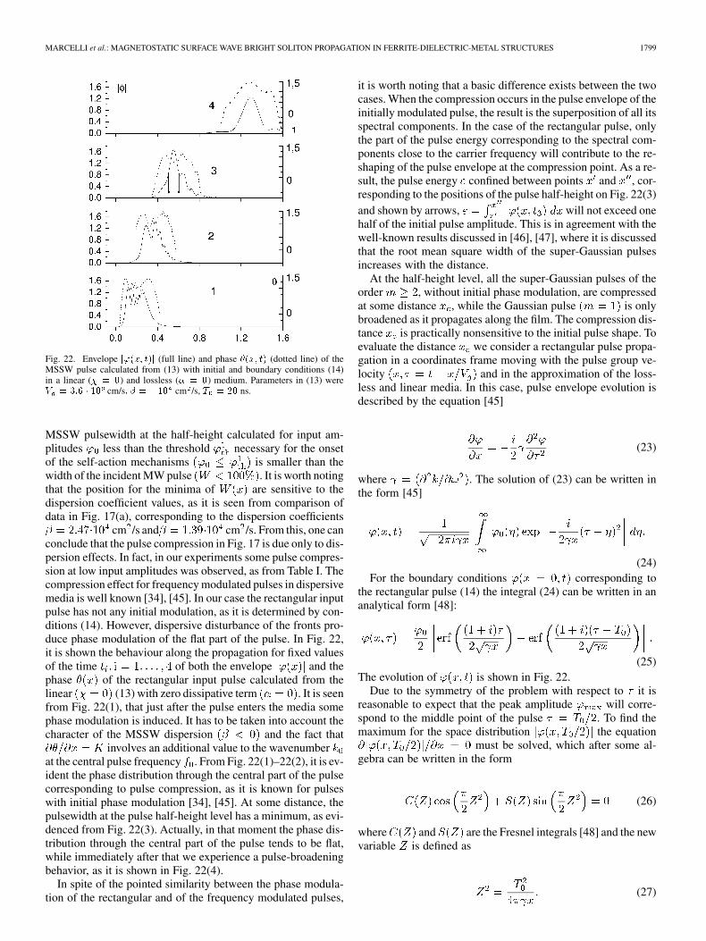
cm /s and cm /s. From this, one canconclude that the pulse compression in Fig. 17 is due only to dis-persion effects. In fact, in our experiments some pulse compres-sion at low input amplitudes was observed, as from Table I. Thecompression effect for frequency modulated pulses in dispersivemedia is well known [34], [45]. In our case the rectangular inputpulse has not any initial modulation, as it is determined by con-ditions (14). However, dispersive disturbance of the fronts pro-duce phase modulation of the flat part of the pulse. In Fig. 22,it is shown the behaviour along the propagation for fixed valuesof the time of both the envelope and thephase of the rectangular input pulse calculated from thelinear (13) with zero dissipative term . It is seenfrom Fig. 22(1), that just after the pulse enters the media somephase modulation is induced. It has to be taken into account thecharacter of the MSSW dispersion and the fact that

involves an additional value to the wavenumberat the central pulse frequency . From Fig. 22(1)–22(2), it is ev-ident the phase distribution through the central part of the pulsecorresponding to pulse compression, as it is known for pulseswith initial phase modulation [34], [45]. At some distance, thepulsewidth at the pulse half-height level has a minimum, as evi-denced from Fig. 22(3). Actually, in that moment the phase dis-tribution through the central part of the pulse tends to be flat,while immediately after that we experience a pulse-broadeningbehavior, as it is shown in Fig. 22(4).

In spite of the pointed similarity between the phase modula-tion of the rectangular and of the frequency modulated pulses,

it is worth noting that a basic difference exists between the twocases. When the compression occurs in the pulse envelope of theinitially modulated pulse, the result is the superposition of all itsspectral components. In the case of the rectangular pulse, onlythe part of the pulse energy corresponding to the spectral com-ponents close to the carrier frequency will contribute to the re-shaping of the pulse envelope at the compression point. As a re-sult, the pulse energy confined between points and , cor-responding to the positions of the pulse half-height on Fig. 22(3)and shown by arrows, will not exceed onehalf of the initial pulse amplitude. This is in agreement with thewell-known results discussed in [46], [47], where it is discussedthat the root mean square width of the super-Gaussian pulsesincreases with the distance.

At the half-height level, all the super-Gaussian pulses of theorder , without initial phase modulation, are compressedat some distance , while the Gaussian pulse is onlybroadened as it propagates along the film. The compression dis-tance is practically nonsensitive to the initial pulse shape. Toevaluate the distance we consider a rectangular pulse propa-gation in a coordinates frame moving with the pulse group ve-locity and in the approximation of the loss-less and linear media. In this case, pulse envelope evolution isdescribed by the equation [45]

(23)

where . The solution of (23) can be written inthe form [45]

(24)For the boundary conditions corresponding to

the rectangular pulse (14) the integral (24) can be written in ananalytical form [48]:

(25)The evolution of is shown in Fig. 22.

Due to the symmetry of the problem with respect to it isreasonable to expect that the peak amplitude will corre-spond to the middle point of the pulse . To find themaximum for the space distribution the equation

must be solved, which after some al-gebra can be written in the form

(26)

where and are the Fresnel integrals [48] and the newvariable is defined as

(27)


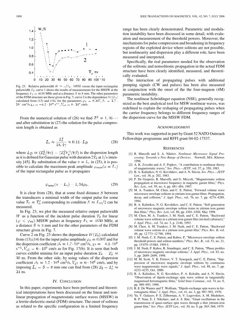
Fig. 23. Relative pulsewidth W = �=T � 100% versus the input rectangularpulsewidth T : curve 1 shows the results of measurements for the MSSW at thefrequency F = 4630MHz and at a distance S � 8 mm. The other parametersof the FDM structure are those given in Fig. 7; curve 2 is the dependenceW (T )calculated from (13) and (14), for the parameters ' = 0:007; � = 1:7 �10 cm /s,� = �8:2 � 10 s ; V = 6 � 10 cm/s.

From the numerical solution of (26) we findand after substitution in (27) the solution for the pulse compres-sion length is obtained as

(28)

where is the dispersion lengthas it is defined for Gaussian pulse with duration at inten-sity [45]. By substitution of the value in (25), it is pos-sible to calculate the maximum peak amplitudeof the input rectangular pulse as it propagates

(29)

It is clear from (28), that at some fixed distance betweenthe transducers a minimal width of the output pulse for somevalue corresponding to condition can bemeasured.

In Fig. 23, we plot the measured relative output pulsewidthas a function of the incident pulse duration for linear

MSSW pulses at frequency MHz, ata distance mm and for the other parameters of the FDMstructure given in Fig. 7.

Curve 2 on Fig. 23 shows the dependence calculatedfrom (13),(14) for the input pulse amplitude and forthe dispersion coefficient cm /s,s cm/s as for Fig. 17(b). It is seen that bothcurves exhibit minima for an input pulse duration

ns. From the other side, by using values of the dispersioncoefficient cm /s, cm/s, and byimposing mm one can find from (28)

ns.

IV. CONCLUSION

In this paper, experiments have been performed and theoret-ical interpretations have been discussed on the linear and non-linear propagation of magnetostatic surface waves (MSSW) ina ferrite-dielectric-metal (FDM) structure. The onset of solitonsas related to the specific configuration in a limited frequency

range has been clearly demonstrated. Parametric and modula-tion instability have been discussed in some detail, with evalu-ation and measurement of the threshold powers. Moreover, themechanisms for pulse compression and broadening in frequencyregions of the exploited device where solitons are not possible,but nonlinearity and dispersion play a different role, have beenmeasured and interpreted.

Specifically, the real parameters needed for the observationof the solitonic and nonsolitonic propagation in the actual FDMstructure have been clearly identified, measured, and theoreti-cally evaluated.

The interaction of propagating pulses with additionalpumping signals (CW and pulses) has been also measuredin conjunction with the onset of the the four-magnon (4M)parametric instability.

The nonlinear Schrödinger equation (NSE), generally recog-nized as the best analytical tool for MSW nonlinear waves, wasredefined to explain the reshaping of propagating pulses whenthe carrier frequency belongs to different frequency ranges ofthe dispersion curve for the MSSW FDM.

ACKNOWLEDGMENT

This work was supported in part by Grant 52 NATO OutreachFellowships programme and RFFI grant 04-02-17537.

REFERENCES

[1] R. Marcelli and S. A. Nikitov, Nonlinear Microwave Signal Pro-cessing: Towards a New Range of Devices. Norwell, MA: Kluwer,1996.

[2] A. K. Zvezdin and A. F. Popkov, “A contribution to nonlinear theoryof magnetostatic waves,” Sov. Phys.—JETP, vol. 57, p. 350, 1983.

[3] B. A. Kalinikos, N. G. Kovshikov, and A. N. Slavin, Sov. Phys.—JETPLett., vol. 38, p. 202, 1983.

[4] P. De Gasperis, R. Marcelli, and G. Miccoli, “Magnetostatic solitonpropagation at microwave frequency in magnetic garnet films,” Phys.Rev. Lett., vol. 59, no. 4, pp. 481–484, 1987.

[5] M. A. Tsankov, M. Chen, and C. E. Patton, “Forward volume wavemicrowave envelope solitons in yttrium iron garnet films: Propagation,decay, and collision,” J. Appl. Phys., vol. 76, no. 7, pp. 4274–4289,1994.

[6] B. A. Kalinikos, N. G. Kovshikov, and C. E. Patton, “Self-generationof microwave magnetic envelope soliton trains in yttrium iron garnetthin films,” Phys. Rev. Lett, vol. 80, pp. 4301–4304, May 1998.

[7] M. Chen, M. A. Tsankov, J. M. Nash, and C. E. Patton, “Backwardvolume wave solitons in a yttrium iron garnet film (invited) (abstract),”J. Appl. Phys., vol. 74, no. 3, p. 2146, 1993.

[8] M. Chen, A. M. Tsankov, J. M. Nash, and C. E. Patton, “Backwardvolume wave soitons in a yttrium iron garnet film,” Phys. Rev. B, vol.49, pp. 12 773–12 790, 1994.

[9] J. M. Nash, C. E. Patton, and Kabos. P, “Microwave-envelope solitonthreshold powers and soliton numbers,” Phys. Rev. B., vol. 51, no. 21,pp. 15 079–15 084, 1995-I.

[10] J. M. Nash, P. Kabos, R. Staudinger, and C. E. Patton, “Phase profilesof microwave magnetic envelope solitons,” J. Appl. Phys., vol. 83, no.5, pp. 2689–2699, 1998.

[11] M. M. Scott, Y. K. Fetisov, V. T. Synogach, and C. E. Patton, “Sup-pression of microwave magnetic envelope solitons by continuouswave magnetostatic wave signals,” J. Appl. Phys., vol. 88, no. 7, pp.4232–4235, Oct. 2000.

[12] B. A. Kalinikos, N. G. Kovshikov, P. A. Kolodin, and A. N. Slavin,“Observation of dipole-exchange spin wave soliton in tangentiallymagnetised ferromagnetic films,” Solid State Commun., vol. 74, no. 9,pp. 989–993, 1990.

[13] R. E. De Wames and T. Wolfram, “Dipole-exchange spin waves in fer-romagnetic films,” J. Appl. Phys., vol. 41, no. 3, pp. 987–992, 1970.

[14] Yu. V. Gulayev, P. E. Zilberman, A. V. Lugovskoi, A. M. Mednikov,B. P. Nam, E. I. Nikolaev, and A. S. Khe, “Giant oscillations in thetransmission of quasi-surface spin waves through a thin yttrium-irongarnet film,” Sov. Phys. JETP Lett., vol. 30, no. 9, pp. 565–568, 1979.


[15] J. D. Adam and S. N. Stitzer, “MSW frequecy selective limiters atUHF,” IEEE Trans. Magn., vol. 40, no. 4, pp. 2844–2846, Jul. 2004.

[16] M. Wu, B. A. Kalinikos, and C. E. Patton, “Generation of dark andbright spin wave envelope soliton trains through self-modulation insta-bility in magnetic films,” Phys. Rev. Lett., vol. 93, no. 15, p. 15 207,2004.

[17] A. D. Boardman and S. A. Nikitov, “To the theory of magnetostaticsurface waves,” Fizika Tverdogo Tela, Sov. Phys. Leningrad, 1989.

[18] S. A. Nikitov, S. Jun, R. Marcelli, and P. DeGasperis, “Modulatiominstability of surface magnetostatic waves in ferromagnetic films,” J.Magn. Magn. Mater., vol. 145, pp. L6–L10, 1995.

[19] V. T. Synogach, Y. K. Fetisov, C. Mathieu, and C. E. Patton, “Ultrashort magnetostatic surface wave pulse formation due to three magnoninteraction,” Phys. Rev. Lett., vol. 85, no. 10, pp. 2184–2187, 2000.

[20] Y. V. Gulayev, P. E. Zilberman, S. A. Nikitov, and A. G. Temiryazev,Solid State Phys., (Sov. Phys. Leningrad), vol. 29, 1987.

[21] P. Kabos, H. Xia, H. Zhang, P. A. Kolodin, and C. E. Patton, “Brillouinlight scattering and magnon wave vector distributions for microwavemagnetic envelop solitons in thin films,” presented at the Int. Symp.Spin Waves, St. Petersburg, Russia, 1998.

[22] A. V. Bagada, G. A. Melkov, A. A. Serga, and A. N. Slavin, “Parametricinteraction of dipolar spin wave solitons with localized electromagneticpumping,” Phys. Rev. Lett., vol. 79, no. 11, pp. 2137–2140, 1997.

[23] P. A. Kolodin, P. Kabos, C. E. Patton, B. A. Kolinikos, N. G.Kovshikov, and M. P. Kostylev, “Amplification of microwave mag-netic envelope solitons in thin yttrium iron garnet films by parallelpumping,” Phys. Rev. Lett., vol. 80, no. 9, pp. 1976–1979, 1998.

[24] A. A. Serga, S. O. Demokritov, S. O. B. Hillebrands, and A. N. Slavin,“Formation of envelope solitons from parametrically amplified andconjugated spin wave pulses,” J. Appl. Phys., vol. 93, no. 10, pp.8758–8760, 2003.

[25] A. V. Kokin and S. A. Nikitov, “Influence of continuous pumpingon magnetostatic spin wave soliton envelope propagation,” Solid StatePhys., vol. 43, no. 5, pp. 851–854, 2001.

[26] A. O. Korotkevich and S. A. Nikitov, “Cross-phase modulation of sur-face magnetostatic spin waves,” JETP, vol. 116, no. 12, p. 2001, 1997.

[27] J. W. Boyle, S. A. Nikitov, A. D. Boardman, and K. Xie, J. Magn.Magn. Mater., vol. 173, p. 241, 1997.

[28] R. Marcelli and S. A. Nikitov, “Magnetostatic surface wave solitonsinduced by cross-phase modulation,” Europhys. Lett., vol. 54, no. 1,pp. 91–97, 2001.

[29] G. T. Kazakov, A. V. Kozhevnikov, and Y. A. Filimonov, “The effectof parametrically excited spin waves on the dispersion and damping ofmagnetostatic surface waves in ferrite films,” JETP, vol. 88, no. 1, pp.174–181, 1999.

[30] T. W. O’Keeffe and R. W. Patterson, “Magnetostatic surface-wavepropagation in finite samples,” J. Appl. Phys., vol. 49, no. 9, pp.4886–4895, 1978.

[31] J. D. Adam, “A broadband microwave signal to noise enchancer,” IEEETrans. Magn., vol. MAG-5, no. 5, pp. 1168–1170, Sep. 1980.

[32] S. N. Stitzer and P. R. Emtage, “Nonlinear microwave signal-pro-cessing devices using thin ferrimagnetic films,” Circ. Syst. SignalProcess., vol. 4, no. 1–2, pp. 227–252, 1985.

[33] H. Suhl, “The theory of ferromagnetic resonance at high signalpowers,” J. Phys. Chem. Solids, vol. 1, pp. 209–227, 1957.

[34] L. A. Vainstein, “Pulse propagation,” Uspechi Phyzicheskich Nauk, vol.118, no. 2, pp. 339–367, 1976.

[35] B. A. Kalinikos, N. G. Kovshikov, and A. N. Slavin, “Effect of mag-netic dissipation on propagation of dipole spin-wave envelope solitonsin yttrium iron garnet films,” IEEE Trans. Magn., vol. 28, no. 5, pp.3207–3209, Sep. 1992.

[36] M. Chen, J. M. Nash, and C. E. Patton, “A numerical study of nonlinearSchrödinger equation solution for microwave soliton in magnetic thinfilms,” J. Appl. Phys., vol. 73, no. 8, pp. 3906–3909, 1993.

[37] A. D. Boardman, S. A. Nikitov, N. A. Waby, R. Putman, H. M. Metha,and R. F. Wallis, “Effect of third-order dispersion on nonlinear magne-tostatic spin waves in ferromagnetic films,” Phys. Rev. B, vol. B.57, p.10667, 1998.

[38] A. S. Kindyak, M. M. Scott, and C. E. Patton, “Numerical analysis ofnonlinear pulse propagation in ferrite-dielectric-metal structure basedon the nonlinear Schrödinger equation with higher order term,” J. Appl.Phys., vol. 93, no. 8, pp. 4739–4745, 2003.

[39] G. M. Dudko, Y. A. Filimonov, A. V. Galishnikov, R. Marcelli, and S.A. Nikitov, “Nonlinear Schrödinger equation analysis of MSSW pulsepropagation in ferrite-dielectric-metal structure,” in Proc. ICM, Rome,Italy, Jul. 27–Aug. 1 2003.

[40] A. A. Galishnikov, G. M. Dudko, and Y. A. Filimonov, “Magnetostatocsurface waves soliton in ferrite-dielectric-metal structure,” Radiotech-nika i electronica, vol. 40, no. 2, pp. 228–234, 2004.

[41] M. P. Kostylev and N. G. Kovshikov, “Excitation, generation and prop-agation of soliton-like spin-wave pulses in ferromagnetic films: Calcu-lations and experiment,” Tech. Phys., vol. 47, no. 11, pp. 1350–1358,2002.

[42] C. J. Mckinstrie and R. Bingham, “The modulation instability of cou-pled waves,” Phys. Fluids B, vol. 1, no. 1, pp. 23–237, 1989.

[43] N. M. Ryskin, “Coupled nonlinear Schrödinger equations for multifre-quency wave packets in a dispersive nonlinear medium,” J. Exp. The-oret. Phys., vol. 79, no. 5, pp. 833–835, 1994.

[44] J. Satsuma and N. Yajima, “Initial value problems of one-dimensionalself modulation of nonlinear waves in dispersive media,” Progr. The-oret. Phys. Supplement, vol. 55, pp. 284–306, 1974.

[45] S. A. Akhmanov, V. A. Vyslouch, and A. S. Chirkin, “Wave packetsself-action in a nonlinear medium and femtosecond laser pulses gener-ation,” Uspechi phyzicheskich nauk, vol. 149, no. 3, pp. 449–509, 1986.

[46] G. Agrawal and M. J. Potasek, “Effect of frequency chirping on theperfomance of optical communication systems,” Opt. Lett., vol. 11, no.5, pp. 318–320, 1986.

[47] D. Anderson and M. Lisak, “Propagation characteristics of the fre-quency-chirped super-Gaussian optical pulses,” Opt. Lett., vol. 11, no.9, pp. 569–571, 1986.

[48] M. Abramowitz and I. A. Stegun, “Handbook of mathematical func-tions,” National Bureau of Standards, Applied mathematics series 55,1964.

Manuscript received January 13, 2005; revised February 3, 2006. Corre-sponding author: R. Marcelli (e-mail: [email protected]).

Magnetostatic surface wave bright soliton propagation in ferrite-dielectric-metal structures

Documents

Transcript of Magnetostatic surface wave bright soliton propagation in ferrite-dielectric-metal structures