A waveform inversion including tilt: method and simple tests

Geophys. J. Int. (2011) 184, 907–918 doi: 10.1111/j.1365-246X.2010.04892.x

GJI

Sei

smol

ogy

A waveform inversion including tilt: method and simple tests

Yuta Maeda,∗ Minoru Takeo and Takao OhminatoEarthquake Research Institute, The University of Tokyo, Japan. E-mail: [email protected]

Accepted 2010 November 13. Received 2010 November 13; in original form 2010 June 25

S U M M A R YA new waveform inversion method is proposed to deal with horizontal seismograms stronglycontaminated by tilt signals, without assumptions regarding tilt motions. Instead of decom-posing the horizontal seismograms into translational and tilt contributions, we realize this taskby calculating the Green’s functions consisting of not only the seismometer’s response to thesynthetic translational motions but also to the synthetic tilt motions. A finite difference method(FDM), which uses a staggered grid and a perfect matched layer (PML) boundary condition, isused to calculate the Green’s functions. This method enables calculation of wavefields whichhave wavelengths of up to 10 times larger than the dimension of the computational grid.Although reflected waves from the numerical boundaries are negligible, comparisons withanalytical solutions evidence errors of up to several per cent. These occur either because thesource-to-receiver distance is small once compared to the grid size, or as a consequence of thehalf-cell difference between the actual free surface and the station location. In addition, in thecase that the free surface is not flat, an error of up to 60 per cent occurs in calculating the tiltmotion, due to the stair-like approximation of topography in the FDM. This latter error canbe reduced to 10 per cent by averaging the tilts at five adjacent cells aligned in the directionof the tilt component, centred on the target grid cell. By applying this algorithm, a waveforminversion can be used to successfully reconstruct the vertical and horizontal seismograms ofvery-long-period (10–30 s) pulses at Asama Volcano, central Japan, despite the fact that thehorizontal seismograms are strongly contaminated by tilt signals.

Key words: Time-series analysis; Inverse theory; Earthquake source observations; Volcanoseismology; Computational seismology; Wave propagation.

1 I N T RO D U C T I O N

Horizontal broad-band seismograms are contaminated by tilt mo-tions because a tilt motion generates a gravitational force whichis equivalent to an inertial force resulting from ground accelera-tion (e.g. Rodgers 1968). For vertical seismograms, this gravita-tional force appears as a second-order term of the tilt angle, mean-ing that it is negligible for ordinary microradian-order tilt motions(e.g. Graizer 2006). In contrast, this force affects horizontal seismo-grams as a first-order term and cannot be neglected under certainobservational conditions, especially in near-field observations ofvolcanoes. For example, Aoyama (2008) demonstrated theoreticallythat the contribution from a tilt motion to a horizontal seismogramis as large as 0.6 times that from a translational motion in the casethat input is an isotropic point source with 60 s duration at a depthof 100 m and that the resultant displacement and tilt are observedby a CMG40T seismometer located 200 m from the epicentre.

∗Now at: National Research Institute for Earth Science and DisasterPrevention, Japan.

Fig. 1 shows a very-long-period (VLP) pulse (e.g. McNutt 2005)observed at the crater rim of Asama Volcano, central Japan (seeFig. 2a for a location map). While the horizontal (upper panel inFig. 1) and vertical (lower panel in Fig. 1) initial pulse shapes fromt = 1090 to 1100 s are similar to each other, a much longer transientsignal from t = 1100 to 1300 s appears only in the horizontalseismogram, suggesting that this transient signal is caused mainly bya tilt motion. Indeed, we observed this pulse at 14 stations (Fig. 2b)at various incidence and azimuthal angles, thereby excluding thepossibility that the transient signal was observed exclusively in thehorizontal seismogram simply because the seismometer was locatedat a node of the vertical component.

Various algorithms have been proposed to decompose horizon-tal seismograms into translational and tilt signals. For example,Wielandt & Forbriger (1999) assumed that a vertical ground dis-placement, a horizontal ground displacement, and a ground tilt allshare the same time functions (with different amplitudes to eachother) in near-field observations. If this assumption is correct, thencontribution from translational motion to the horizontal seismo-gram is expected to be proportional to the vertical seismogram,and contribution from tilt motion to the horizontal seismogram is

C© 2010 The Authors 907Geophysical Journal International C© 2010 RAS

Geophysical Journal InternationalD

ownloaded from

https://academic.oup.com

/gji/article/184/2/907/594741 by guest on 22 June 2022

908 Y. Maeda, M. Takeo and T. Ohminato

Figure 1. Very-long-period (VLP) pulse at Asama Volcano, central Japan, provided as an example of a seismogram strongly contaminated by tilt motion. Theupper panel shows an east–west (nearly radial) seismogram and the lower panel shows a vertical seismogram recorded at station KAE. A pulse from t = 1090to 1100 s, which appears in both seismograms, can be interpreted as reflecting a translational motion. A much longer transient signal, from t = 1100 to 1300 s,appears only in the horizontal seismogram, indicating that this signal is the seismometer’s response to a tilt motion. Because a gravitational force generated byground tilting is a second-order term in vertical seismograms, the degree of contamination of the vertical seismogram resulting from a microradian-order tiltmotion is 0.000001 times as small as that of a horizontal seismogram; consequently, it can be neglected. Therefore, the vertical signal from t = 1100 to 1130 sis also a translational signal.

Figure 2. (a) Location of Asama Volcano (black triangle), central Japan. (b) Station layout at the summit area of Asama Volcano. Squares, circles, diamonds,and triangles indicate Guralp CMG-3T 360 s sensors, Nanometrics Trillium 120 s sensors, Guralp CMG-3T 100 s sensors, and Nanometrics Trillium 40 ssensors, respectively. Contour interval is 20 m, and station KAE is located at 2568 m above sea level.

expected to be proportional to the twice integration of the verti-cal seismogram; thus the total horizontal seismogram is expectedto be the weighted sum of a vertical seismogram and its doubleintegration of the same station. The weighting factors multipliedwith the vertical seismogram and with its double integration arethe relative amplitudes of horizontal translational motion and tiltmotion to the vertical ground motion, respectively, which can bedetermined by a least squares fitting of the real horizontal seismo-gram and the synthetic seismogram (the weighted sum). Zahradnik& Plesinger (2005) made the assumption that a ground tilt motionitself is short enough to be approximated as a step function. Basedon this assumption, the timing and amplitude of the step can be

determined by minimizing the fitting error between an observedtransient signal and a synthetic response of the seismometer to thestep-like tilt. Graizer (2006) considered that horizontal seismogramsare dominated by translational signals at high frequencies and bytilt signals at low frequencies. Given this scenario, a high-pass fil-ter would return an approximated translational seismogram, whilea low-pass filter would return an approximated tilt seismogram.A corner frequency of these filters can be determined by compar-ing horizontal and vertical Fourier amplitude spectra if we assumesimilar spectra shapes between horizontal and vertical translationalmotions. In these algorithms, however, some assumption is requiredregarding time functions or the Fourier spectra of translational and

C© 2010 The Authors, GJI, 184, 907–918

Geophysical Journal International C© 2010 RAS

Dow

nloaded from https://academ

ic.oup.com/gji/article/184/2/907/594741 by guest on 22 June 2022

A waveform inversion including tilt 909

tilt motions. Such assumption was justified in previous papers byreferring to independently observed tilt values, as well as the excel-lent match between observed and synthetic seismograms calculatedbased on the assumption. However, there may be cases where ei-ther direct observations of tilt are absent or where the assumptionfail to produce an excellent match. Consequently, a new method isrequired to deal with cases in which horizontal seismograms arecontaminated by tilt motions.

In this paper, we propose a new moment-tensor inversion methodto deal with horizontal seismograms contaminated by tilt motions,without making any assumptions regarding tilt motions. Our ideais to include the effect of tilt motions into the Green’s functionsinstead of decomposing the horizontal seismograms into transla-tional and tilt responses. We realized this idea by introducing aperfect matched layer (PML) boundary condition (Festa & Nielsen2003) into the finite difference method (FDM) code developed byOhminato & Chouet (1997). In Section 2, we explain the basic ideaof the inversion and describe the FDM code using a PML boundary,as used to calculate synthetic tilt motions. An explicit formulationof the FDM code is described in Appendix A. In Section 3, weshow the results of numerical tests of the FDM code, revealing itsaccuracy and limitations. In Section 4, we briefly describe the ap-plication of the method to waveform inversion. The full applicationof the new inversion method and the obtained results are describedin a future paper.

2 N E W M O M E N T - T E N S O R I N V E R S I O NA L G O R I T H M T O D E A L W I T HH O R I Z O N TA L S E I S M O G R A M SC O N TA M I NAT E D B Y T I LT

A source time function of the (p, q) component of a moment-tensorpoint source Mpq(t) generates the following displacement

U transn (t) = Mpq (t) ∗ G trans

np,q (t), (1)

where p is the direction of force, q is the direction of the arm ofthe moment, n is a consecutive number which uniquely indicatesa combination of station and component, t is time, ‘,q’ is a partialderivative with respect to the coordinate xq, ‘∗’ is the convolutionwith respect to time and Gnp(t) is the nth component of Green’sfunction at a station excited by a pth direction unit impulse at asource (e.g. Ohminato et al. 1998). Here, the summation conventionis applied for repeated subscripts. The superscript ‘trans’ indicatesthat the displacement Un(t) and the Green’s functions Gnp,q(t) aretranslational. The Fourier transform of eq. (1) is

U transn (ω) = Mpq (ω)G trans

np,q (ω), (2)

where ω denotes the angular frequency. Previous moment-tensorinversions are based on eq. (2) with an assumption that the Fouriertransform of observed seismograms U obs

n (ω) can be approximatedas

U obsn (ω) ∼ U trans

n (ω), (3)

by neglecting tilt motions. A key aspect of this study is the extensionof eq. (3) to a more generalized equation, as follows

U obsn (ω) = U trans

n (ω)I transn (ω) + θn(ω)I tilt

n (ω) (4)

which is applicable in cases where the contribution of tilt motion tothe observed seismogram cannot be neglected. Here, I trans

n (ω) andI tilt

n (ω) represent the seismometer’s translational and tilt responses,

respectively, and θn(ω) is the Fourier transform of the ground tiltmotion, which can be written as

θn(ω) = Mpq (ω)G tiltnp,q (ω), (5)

where G tiltnp,q is the Green’s function of tilt motion; that is, tilt motion

generated by an impulsive source. Substituting eqs (2) and (5) intoeq. (4) yields

U obsn (ω) = Mpq (ω)

[G trans

np,q (ω)I transn (ω) + G tilt

np,q (ω)I tiltn (ω)

]. (6)

For practical use, the following equation is more convenient

U obsn (ω)S0(ω) = Mpq (ω)

[{S0(ω)G trans

np,q (ω)}

I transn (ω)

+ {S0(ω)G tilt

np,q (ω)}

I tiltn (ω)

],

(7)

where S0(ω) is the Fourier transform of an arbitrary source timefunction used to calculate a synthetic displacement S0(ω)G trans

np,q (ω)and a synthetic tilt S0(ω)G tilt

np,q(ω).I trans

n (ω) can be obtained from the poles and zeroes informationof the seismometer, and I tilt

n (ω) for horizontal seismograms can beobtained by recognizing that a tilt motion θ (t) generates a grav-itational force −mg sin θ (t) ∼ −mgθ (t), where m is the mass ofthe seismometer and g is gravitational acceleration. This gravita-tional force is equivalent to an inertial force generated by a groundacceleration gθ (t), or by a ground displacement, as follows∫

dt

∫ t

0dt ′gθ (t ′). (8)

The Fourier transform of eq. (8) is gθ (ω)/(iω)2, where i is theimaginary unit. Therefore, a seismometer’s tilt response I tilt

n (ω) canbe written as

I tiltn (ω) = g

(iω)2I trans

n (ω) (for horizontal components). (9)

For vertical seismometers, a tilt motion θ (t) generates a gravitationalforce with an order of θ (t)2 (e.g. Graizer 2006), which appears to besufficiently small for ordinary microradian-order tilt motions; thus,

I tiltn (ω) ∼ 0 (for vertical components). (10)

For calculations of the synthetic displacement S0(ω)G transnp,q (ω) and

the synthetic tilt S0(ω)G tiltnp,q(ω) for long-period earthquakes in the

near-field of volcanoes, which is a typical setting in which strongcontamination by tilt signals occurs (e.g. Wielandt & Forbriger1999; Aoyama & Oshima 2008), a synthetic time trace that is suf-ficiently long to cover the duration of the event must be calculatedusing 3-D topography and a sufficiently small grid size to expressthe volcano topography and the wavefield in the near-field. Calcu-lation of long synthetic time traces requires a large computationalvolume or an efficient absorbing boundary condition to avoid con-tamination by waves reflected from model boundaries. However,a large computational volume appears unrealistic, at least for thevery-long-period earthquakes recorded at Asama Volcano (Fig. 1),where the grid size must be as small as 10 m and the computationalvolume must be as large as 20 km × 20 km × 10 km in the casethat we use an insufficient absorbing boundary condition, whichrequires up to 4 × 109 grid cells. Therefore, an efficient absorbingboundary condition is required in addition to consideration of anarbitrary 3-D topography. Ohminato & Chouet (1997) developeda FDM code relevant to this latter requirement. However, it usesClayton’s first-order absorbing boundary condition (Clayton &Engquist 1977), which is somewhat inefficient.

Here, we employed the PML absorbing boundary proposedby Festa & Nielsen (2003) and combined it with Ohminato and

C© 2010 The Authors, GJI, 184, 907–918


Dow




Chouet’s (1997) staggered-grid FDM algorithm. In the PML algo-rithm, the computational volume is bounded by the PML layer, forwhich strong absorption is realized by replacing ∂

∂t , a partial deriva-tive with respect to time, with ∂

∂t +α, where α is a positive constantwith respect to time. The explicit formulation of the present algo-rithm is described in Appendix A. The proposed algorithm does notconsider seismic attenuation Q or rigid body rotations. The directresults of the calculation are velocity and tilt-rate. Displacementand tilt can be obtained by integrating the results with respect totime.

The results of numerical tests are described in the next sec-tion, revealing that the present approach can be used to calcu-late the synthetic displacements S0(ω)G trans

np,q (ω) and synthetic tiltsS0(ω)G tilt

np,q(ω) with an error of ∼10 per cent if the values are calcu-lated at an epicentral distance of 200–500 m and using a grid sizeof 10 m for a 5-s-long source located at a depth of ∼200 m. Theerror is derived mainly from a discretization effect, with contami-nation from the PML layer making a much smaller contribution. Insummary, it is possible to calculate all the factors on the both sidesof eq. (7) except for Mpq(ω); thus, we can invert eq. (7) to obtainthe moment-tensor solution Mpq(ω).

3 N U M E R I C A L T E S T SO F T H E F D M C O D E

3.1 Synthetic displacements in a homogeneousinfinite medium

To assess the efficiency of absorption in the PML layer, we cal-culated a synthetic velocity wavefield in a homogeneous infinite3-D medium using the FDM code proposed in this study. A 1 N mpoint-source dipole having the following source time function

S0(t) =

⎧⎪⎪⎪⎨⎪⎪⎪⎩

0 (for t < 0)

10(

tτp

)3− 15

(t

τp

)4+ 6

(t

τp

)5(for 0 � t � τp)

1 (for τp < t)

(11)

with τ p = 5 s was placed at the centre of the computational volume.This function is the unique polynomial of the minimum possibledegree which satisfies the following conditions: (1) zero beforet = 0, (2) unity after t = τ p, (3) monotone and (4) the secondorder derivatives are continuous. Conditions (1) and (2) indicatethat this source time function is a quasi-static one when seen in along timescale, which is an advantage to compare the calculationresults with analytical solutions such as Mogi (1958). In addition,since many of the very-long-period velocity pulses, including thoseof Asama Volcano (Fig. 1), are one-sided and are observed in near-field, source time functions of them are expected to be similarto eq. (11). Many of the very-long-period pulses are consideredto be generated by volumetric increase caused by vaporization ofliquid, degassing, or similar phenomena, generating a static momentrelease at the source. Condition (3) is only for a simplification.Condition (4) is required because we calculate the velocities whosefar-field terms are proportional to second-order derivatives of thesource moment function. Other parameters in this calculation areas follows: P-wave velocity V p = 2 km s−1, S-wave velocity V s =V p/

√3, density ρ = 2.5 kg m−3, grid size of 20 m, time step of

0.002 s, and source-to-PML distance of 500 m in all directions.Under these conditions, reflected waves from the PML layers arrivewithin 1 s, throughout the entire computational volume.

Fig. 3 shows a series of velocity snapshots obtained by the FDMcalculation, on a x–y section that contains the source location. Here,the x-component of ground velocity, which is generated by a forcedipole at (0, 0) oriented along the x-axis, is shown by colour scale.The velocity decrease observed between t = 2.5 and 5 s is causedby a decrease in the source moment-rate intensity rather than re-flection from the numerical boundary. Although residual velocityis observed in the PML region after t = 5 s, it does not appear topropagate into the computational volume and it gradually attenu-ates with time. This result demonstrates that the wavefield is wellabsorbed in the PML region and that only small waves are reflectedfrom numerical boundaries.

The solid lines in Fig. 4 indicate x-component of ground dis-placements at some locations on Fig. 3, obtained by integrating thevelocities with respect to time. The results are compared with ana-lytical solution of eq. (4.29) in Aki & Richards (2002), as indicatedby dotted lines. Panels (c) and (d) show displacements at (400, 0)and (200, 200), respectively, where excellent fits were obtained.The fit is slightly less accurate at [200, 0; panel (b)] and again soat [100, 0; panel (a)], mainly because number of grid cells betweenthe source and the receiver is insufficient to express the wavefield.We conducted similar calculations for all the six moment tensor andthree single force source mechanisms. In all cases, a high level ofaccuracy was obtained in the FDM calculations for receivers locatedfarther than 10 grid cells from the source.

3.2 Synthetic displacements on a flat surfaceof a homogeneous half-space

Fig. 5 compares the synthetic displacements near a flat free surfaceof a homogeneous half-space medium obtained with the modifiedFDM code and those obtained by the discrete wavenumber method(DWM) proposed by Takeo (1985). In the FDM calculation, a 10 mgrid and a 0.001 s time interval were adopted, and an isotropicsource was applied at a depth of 505 m from the free surface; otherconditions were the same as in the previous calculation. We areunable to obtain the FDM result at the free surface because thezero-traction free surface condition is implemented along the gridinterface, whereas the velocities (and displacements) are definedat the centre of the grid cell. Instead, we calculated the horizontal(radial) displacements at depths from 5 m (a half grid) to 35 m witha 10 m interval (solid lines in Fig. 5). In contrast, the DWM codeof Takeo (1985) yields the displacements only at the free surface.The green and blue dotted lines in the figure indicate the radialdisplacements at the free surface, as obtained by the DWM codeand using the same isotropic source as FDM at depths of 500 and510 m from the free surface, respectively. The epicentral distanceis 200 m for all the lines in Fig. 5.

We can imagine a displacement at the surface in the FDM cal-culation by extrapolating the solid lines in Fig. 5. This imaginaryline probably approaches near the mid-points of the green and bluedotted lines in the figure. In addition, if we use DWM to calcu-late a displacement at the surface caused by an isotropic source ata depth of 505 m, the result would probably be located near themid-point of these dotted lines. Thus, the displacements obtainedby FDM and DWM are consistent with each other. Fig. 5 also showsthe difference in displacement (to within several per cent) betweendisplacement at the surface and at 5 m below the free surface. Con-sequently, in the case that a 10 m grid is used, an error of several percent cannot be avoided in the FDM calculation for a source depthof 500 m and an epicentral distance of 200 m. We found that thiseffect is smaller for vertical displacements for the same geometry.

C© 2010 The Authors, GJI, 184, 907–918


Dow




Figure 3. Velocity snapshots obtained from the FDM simulation for an infinite homogeneous space with V p = 2 km s−1, V s = V p/√

3 and ρ = 2.5 kg m−3.Time of each snapshot is indicated at the top of each panel. The calculation was conducted in a 3-D medium, from which the figure shows a x–y cross sectionthat contains the source location. This figure represents the x-component of ground velocity generated by a force dipole of 1 N m at (0, 0) oriented along thex-axis. The boundary between the computational volume and the PML region is indicated by the rectangle in panel t = 0.0 s.

Figure 4. The x-component of ground displacements obtained from thesame calculation as that shown in Fig. 3. The solid lines indicate the FDM re-sults; dotted lines indicate analytical solution of eq. (4.29) in Aki & Richards(2002). The receiver locations in each panel are as follows: (a) (100, 0), (b)(200, 0), (c) (400, 0) and (d) (200, 200) in Fig. 3. Arrows in each panel in-dicate the arrival times of reflected waves from the nearest PML boundary.

Figure 5. Horizontal (radial) displacements obtained with the modifiedfinite-difference method (FDM; solid lines) and by the discrete wavenumbermethod (DWM; dotted lines) proposed by Takeo (1985) in a homogeneoushalf-space. The source depth of the FDM calculation is 505 m, and thereceiver depths for the red, cyan, magenta and green solid lines are 5 (a half-grid), 15, 25 and 35 m, respectively. For DWM calculation, the receivers lieat the free surface, and the source depths for the green and blue dotted linesare 500 and 510 m, respectively.

C© 2010 The Authors, GJI, 184, 907–918


Dow




Figure 6. Comparison of the tilts calculated by the FDM code proposed in this paper and the analytical solution provided by Mogi (1958). An isotropic sourceof 1 N m was applied at a depth of 195 m from the horizontal surface. The spatial distributions of x-component tilts ∂U z

∂x are compared along the x-axis. Thered line indicates the final tilt (t = 10 s) at the surface and the green dotted line indicates the final tilt at a half-grid below the surface, both obtained from theFDM code. The blue dotted line indicates the analytical solution proposed by Mogi (1958).

3.3 Synthetic tilts on a flat surface of a homogeneoushalf-space

Fig. 6 compares the final tilts calculated by the FDM code with thoseof the analytical solution proposed by Mogi (1958). An isotropicsource of 1 N m was applied at a depth of 195 m in a half-spacewith V p = 2 km s−1, V s = V p/

√3 and ρ = 2500 kg m−3. In

the FDM simulation, a 10 m grid and 0.001 s time interval wereadopted. The PML boundary was placed 500 m from the sourcein the horizontal direction and at a depth of 400 m from the freesurface. The source time function of eq. (11) with τ p = 5 s wasapplied. In this case, tilt-rate functions converged to zero before t =10 s; thus, we integrated these tilt-rate functions with respect to timeto obtain tilt functions, and then adopted the tilt values at t = 10 s asthe final tilts. These final tilts can be calculated at each point on thefree surface and can then be compared with the analytical solutionproposed by Mogi (1958). Fig. 6 show the spatial distributions ofx-components of the final tilts along the x-axis, as obtained by theFDM code (red line) and by the analytical solution (blue dottedline), revealing a near-perfect match. The green dotted line in Fig. 6indicates the final tilt at a half-grid below the surface, which isused in the real inversions. This line is slightly different from theanalytical solution at the surface because the location of calculatedtilt is by a half-grid different from that of the analytical solution.However, this difference is smaller than the mismatch in Fig. 5because the tilt is a spatial derivative of a vertical displacement,and the difference in the vertical displacement caused by a half-gridmismatch between a station and surface location is smaller than thatin the horizontal.

3.4 Synthetic tilts on a constantly inclined surfaceof a homogeneous half-space

We calculated synthetic tilts on a constantly inclined surface witha ∼10◦ slope (dashed line in Fig. 7b) generated by an isotropic

source whose location is indicated by the grey circles in Figs 7(a)and (b). Strictly, our FDM simulation was conducted using thetopography indicated by the solid line in Fig. 7(b), and we calculatedthe tilt motions at a half-grid below the free surface. Other structuralconditions and the source time function are identical to those in theprevious tests.

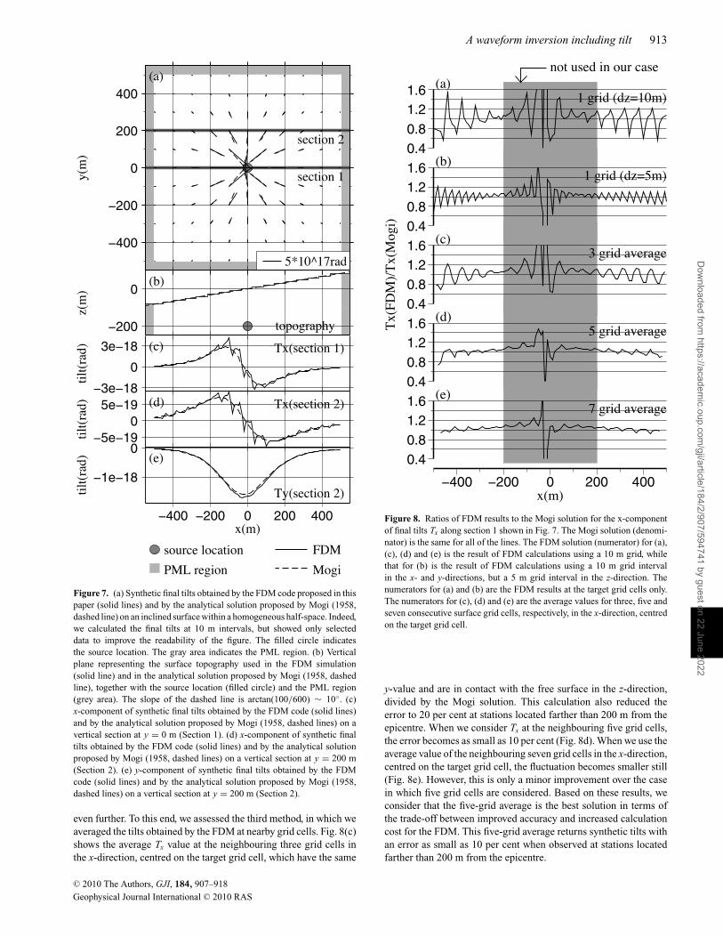
Fig. 7(a) compares the spatial distribution of the final tilts ob-tained by the FDM code (solid lines) and those obtained by theMogi model (dashed lines). The final tilts on vertical sections ofy = 0 m (Section 1) and y = 200 m (Section 2) are shown inFigs 7(c)–(e). The x-components of the final tilts (Tx) obtained bythe FDM simulation fluctuate along the x-axis, whose pattern isconsistent with a stair-like topography. The y-components of thefinal tilts (Ty) obtained by the FDM simulation show minor fluctu-ations, but they systematically deviate from the Mogi solution byseveral per cent. For observations at stations located farther than200 m from the epicentre, this deviation of Ty is minor and the erroris derived mainly from Tx.

The degree of error in Tx along the x-axis is more clearly seenwhen displayed as a ratio to Mogi’s solutions, as shown in Fig. 8(a).The error is as large as 60 per cent, even at stations located as faras 400 m from the source. To suppress this large error and to obtainmore precise tilt by the FDM code, we evaluated three methods. Thefirst method involved the use of a higher-order approximation of thespatial differentiation of the vertical displacements to obtain the tilts;however, this method resulted in greater fluctuations, probably dueto real differences in tilt motions between the stair-like topographyand the smooth slope. The second method involved performingthe FDM calculations using a finer grid size. Fig. 8(b) shows theresult obtained using the same 10 m grid size in the x- and y-directions while using a smaller 5 m grid size in the z-direction. Thefluctuations are reduced to 20 per cent at stations located farther than200 m from the epicentre. However, because the real calculation usesa more complicated topography with locally steeper slopes whichmay amplify the fluctuations, the fluctuations need to be minimized

C© 2010 The Authors, GJI, 184, 907–918


Dow




Figure 7. (a) Synthetic final tilts obtained by the FDM code proposed in thispaper (solid lines) and by the analytical solution proposed by Mogi (1958,dashed line) on an inclined surface within a homogeneous half-space. Indeed,we calculated the final tilts at 10 m intervals, but showed only selecteddata to improve the readability of the figure. The filled circle indicatesthe source location. The gray area indicates the PML region. (b) Verticalplane representing the surface topography used in the FDM simulation(solid line) and in the analytical solution proposed by Mogi (1958, dashedline), together with the source location (filled circle) and the PML region(grey area). The slope of the dashed line is arctan(100/600) ∼ 10◦. (c)x-component of synthetic final tilts obtained by the FDM code (solid lines)and by the analytical solution proposed by Mogi (1958, dashed lines) on avertical section at y = 0 m (Section 1). (d) x-component of synthetic finaltilts obtained by the FDM code (solid lines) and by the analytical solutionproposed by Mogi (1958, dashed lines) on a vertical section at y = 200 m(Section 2). (e) y-component of synthetic final tilts obtained by the FDMcode (solid lines) and by the analytical solution proposed by Mogi (1958,dashed lines) on a vertical section at y = 200 m (Section 2).

even further. To this end, we assessed the third method, in which weaveraged the tilts obtained by the FDM at nearby grid cells. Fig. 8(c)shows the average Tx value at the neighbouring three grid cells inthe x-direction, centred on the target grid cell, which have the same

Figure 8. Ratios of FDM results to the Mogi solution for the x-componentof final tilts Tx along section 1 shown in Fig. 7. The Mogi solution (denomi-nator) is the same for all of the lines. The FDM solution (numerator) for (a),(c), (d) and (e) is the result of FDM calculations using a 10 m grid, whilethat for (b) is the result of FDM calculations using a 10 m grid intervalin the x- and y-directions, but a 5 m grid interval in the z-direction. Thenumerators for (a) and (b) are the FDM results at the target grid cells only.The numerators for (c), (d) and (e) are the average values for three, five andseven consecutive surface grid cells, respectively, in the x-direction, centredon the target grid cell.

y-value and are in contact with the free surface in the z-direction,divided by the Mogi solution. This calculation also reduced theerror to 20 per cent at stations located farther than 200 m from theepicentre. When we consider Tx at the neighbouring five grid cells,the error becomes as small as 10 per cent (Fig. 8d). When we use theaverage value of the neighbouring seven grid cells in the x-direction,centred on the target grid cell, the fluctuation becomes smaller still(Fig. 8e). However, this is only a minor improvement over the casein which five grid cells are considered. Based on these results, weconsider that the five-grid average is the best solution in terms ofthe trade-off between improved accuracy and increased calculationcost for the FDM. This five-grid average returns synthetic tilts withan error as small as 10 per cent when observed at stations locatedfarther than 200 m from the epicentre.

C© 2010 The Authors, GJI, 184, 907–918


Dow




4 A P P L I C AT I O N O F T H E I M P ROV E DM E T H O D T O WAV E F O R M I N V E R S I O N

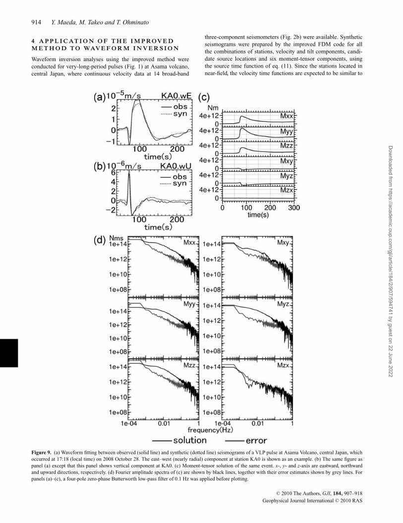
Waveform inversion analyses using the improved method wereconducted for very-long-period pulses (Fig. 1) at Asama volcano,central Japan, where continuous velocity data at 14 broad-band

three-component seismometers (Fig. 2b) were available. Syntheticseismograms were prepared by the improved FDM code for allthe combinations of stations, velocity and tilt components, candi-date source locations and six moment-tensor components, usingthe source time function of eq. (11). Since the stations located innear-field, the velocity time functions are expected to be similar to

Figure 9. (a) Waveform fitting between observed (solid line) and synthetic (dotted line) seismograms of a VLP pulse at Asama Volcano, central Japan, whichoccurred at 17:18 (local time) on 2008 October 28. The east–west (nearly radial) component at station KA0 is shown as an example. (b) The same figure aspanel (a) except that this panel shows vertical component at KA0. (c) Moment-tensor solution of the same event. x-, y- and z-axis are eastward, northwardand upward directions, respectively. (d) Fourier amplitude spectra of (c) are shown by black lines, together with their error estimates shown by grey lines. Forpanels (a)–(c), a four-pole zero-phase Butterworth low-pass filter of 0.1 Hz was applied before plotting.

C© 2010 The Authors, GJI, 184, 907–918


Dow




moment-rate time functions. Eq. (11) was chosen because its time-derivative (the moment-rate time function) seems to have similarwaveform to the velocity seismogram indicated in the lower panelof Fig. 1. While it would be identical to make use of τ p in eq. (11) asnear as the duration of velocity pulse in the real seismogram (10–20s), τ p = 5 s was adopted in order to save calculation time. As isindicated in eq. (7), the source time function used to calculate thesynthetic seismograms is eliminated by convolving it with the ob-served data. Also, the inversion is conducted in frequency domain,where all the discretized frequency contents of the moment-tensorsolution are obtained independently. Thus, theoretically, the choiceof the source time function does not affect the inversion result.

A special care must be taken in preparing the data-kernel. Becausethe calculation of the seismometer’s tilt response includes a doubleintegration with respect to time, a large value is generated at the endof the time window, equivalent to a very large step. Convolution ofthe poles and zeroes of the seismometer in the frequency domainwith this doubly integrated waveform results in a step-responsefunction at the beginning of the time window with a much greateramplitude than that of the real signal. Note that this problem cannotbe avoided simply by using a long time window because this resultsin a larger step at the end of the window. In addition, this problemcannot be avoided by tapering because of the large magnitude ofthe artificial signal. To overcome this problem, it is necessary tofirst prepare a sufficiently long sequence of dummy zeroes at the

beginning of the synthetic tilt waveforms, then to conduct the doubleintegration and convolution operations, and finally to remove thatpart of the time window contaminated by the artificial signal.

Fig. 9 is an extracted result of the inversion thus obtained; fullresults are indicated in a future paper. Figs 9(a) and (b) shows the fitbetween observed (solid lines) and synthetic (dotted lines) seismo-grams, indicating that both the horizontal [panel (a)] and vertical[panel (b)] seismograms are well reconstructed. Fig. 9(c) showsthe moment-tensor time function, consisting of initial rapid infla-tion phase and the following gradual deflation phase. Again, this isthe moment-tensor component itself; not convolved with the timefunction of eq. (11). All the six moment-tensor components werederived with sufficient resolution. They have similar time functionsto each other, indicating that the source mechanism does not seri-ously change with time. The source mechanism can be interpretedas a synchronized expansion of a tensile-crack and a cylinder, lo-cated under the northern part of the crater, near the upper end of thevolcanic earthquake hypocentres (Fig. 10). Fig. 9(d) is the Fourierspectrum of the moment-tensor solution (black lines), together withits error estimate (grey lines). Here, roughly speaking, the errorwas estimated by multiplying the inverse of the Green’s functionswith the error of data itself; thus error caused by uncertainty ofthe Green’s functions are not included in the gray lines. Since theGreen’s functions seem to have uncertainties of up to 10 per centfrom our numerical tests described in the previous sections, it might

Figure 10. Relationship among the inversion results, surface topography, and hypocentres of other volcanic earthquakes. The upper left panel, lower panel, andright panel show projections into the horizontal cross-section, an east–west cross-section and a north–south cross-section, respectively. Topographies plottedin the vertical sections are those along the black dashed lines in the map view. Orange solid quadrangle indicates the source tensile crack, while red dottedline indicates a symmetry axis of the source cylinder. Hypocentres are shown for ordinary earthquakes with latitudes (lower panel) and longitudes (right-handpanel) within 300 m of the black dashed lines and with altitudes (upper left-hand panel) higher than 500 m above sea level. These hypocentres were determinedusing the double-difference method proposed by Waldhauser & Ellsworth (2000). Because the installation of summit stations in early 2007 November mayhave affected the hypocentre distributions, different symbols are used for data collected before and after installation of the stations.

C© 2010 The Authors, GJI, 184, 907–918


Dow




map to uncertainty of ∼10 per cent in the black lines of Fig. 9(d).On the other hand, difference between the moment-tensor spectra[black lines in Fig. 9(d)] and their errors (grey lines in Fig. 9d) aremeaningfully larger than 10 per cent in a frequency range between0.002 and 0.1 Hz (except for Mzx), indicating that the moment-tensor solution was well reconstructed in this frequency range. Mzx

is no larger than error.

5 C O N C LU S I O N

We developed a new moment-tensor inversion method applicableto seismograms strongly contaminated by tilt motions. The methodinvolves calculating the Green’s functions of the tilt motions, madepossible by adopting the Perfect Matched Layer absorbing bound-aries proposed by Festa & Nielsen (2003). The results of numericaltests indicate negligible contamination from reflected waves fromthe numerical boundaries, even in the case where the wavelengthis 10 times as long as the computational volume. However, errorsof up to 10 per cent occur as a result of either the small source-to-receiver distance compared with the grid size or as a result of thehalf-grid difference between the free surface and the station loca-tion. In addition, an error of up to 60 per cent occurs in synthetictilts as a result of a stair-like topography approximation. This errorcan be reduced to 10 per cent by averaging the synthetic tilts at fiveadjacent grid cells in the direction of the tilt component, centred onthe target grid cell. In preparing the data-kernel of the inversion,it is necessary to ensure sufficient zero padding before the doubleintegration of the Green’s functions of the tilt motions, and to theneliminate the artificial signals at the beginning of the seismometer’sresponse. With a use of the proposed algorithm, both horizontal andvertical seismograms were well reconstructed by inversion, deriv-ing a reliable moment-tensor time function in a frequency rangebetween 0.002 and 0.1 Hz.

A C K N OW L E D G M E N T S

Professor Bernard Chouet and another anonymous reviewer pro-vided constructive comments. MT was partially supported from theGrant-in-Aid for Scientific Research, Japan Society for Promotionof Science (KAKENHI) No. 22540431.

R E F E R E N C E S

Aki, K. & Richards, P., 2002. Quantitative Seismology, 2nd edn, UniversityScience Books, Sausalito, CA.

Aoyama, H., 2008. Simplified test on tilt response of CMG40T seismome-ters, Bull. Volcanol. Soc. Jpn., 53, 35–46.

Aoyama, H. & Oshima, H., 2008. Tilt change recorded by broad-band seismometer prior to small phreatic explosion of Meakan-dake volcano, Hokkaido, Japan, Geophys. Res. Lett., 35, L06307,doi:10.1029/2007GL032988.

Clayton, R. & Engquist, B., 1977. Absorbing boundary conditions for acous-tic and elastic wave equations, Bull. seism. Soc. Am., 67, 1529–1540.

Festa, G. & Nielsen, S., 2003. PML absorbing boundaries, Bull. seism. Soc.Am., 93, 891–903.

Graizer, V., 2006. Tilts in strong ground motion, Bull. seism. Soc. Am., 96,2090–2102.

McNutt, S., 2005. Volcanic seismology, Ann. Rev. Earth planet Sci., 32,461–491.

Mogi, K., 1958. Relations between the eruptions of various volcanoes andthe deformations of the ground surface around them, Bull. Earthq. Res.Inst., 36, 99–134.

Ohminato, T. & Chouet, B., 1997. A free-surface boundary condition forincluding 3D topography in the finite-difference method, Bull. seism. Soc.Am., 87, 494–515.

Ohminato, T., Chouet, B., Dawson, P. & Kedar S., 1998. Waveform inversionof very long period impulsive signals associated with magmatic injectionbeneath Kilauea Volcano, Hawaii, J. geophys. Res., 103, 23 839–23 862.

Rodgers, P.W., 1968. The response of the horizontal pendulum seismometerto Reileigh and Love waves, tilt, and free oscillations of the Earth, Bull.seism. Soc. Am., 58, 1384–1406.

Takeo, M., 1985. Near-field synthetic seismograms taking into account theeffects of anelasticity—the effects of anelastic attenuation on seismo-grams caused by a sedimentary layer, Papers Meteorol. Geophys., 36,245–257.

Waldhauser, F. & Ellsworth, W.L., 2000. A double difference earthquakelocation algorithm: method and application to the Northern HaywardFault, California, Bull. seism. Soc. Am., 90, 1353–1368.

Wielandt, E. & Forbriger, T., 1999. Near-field seismic displacement and tiltassociated with the explosive activity of Stromboli, Annali di Geofisica,42, 407–416.

Zahradnik, J. & Plesinger, A., 2005. Long-period pulses in broadbandrecords of near earthquakes, Bull. seism. Soc. Am., 95, 1928–1939.

A P P E N D I X A : E X P L I C I TF O R M U L AT I O N S O F T H E M O D I F I E DF D M C O D E

The equation of motion and the constitutive law of an isotropicelastic medium are

ρui =3∑

k=1

τik,k + fi (A1)

and

τi j =3∑

p,q=1

ci jpq u p,q , (A2)

respectively, where ρ is density, ui is the ith component of dis-placement, τ ik is the (i,k) component of the stress tensor, fi is theith component of the body force, ‘ ˙ ’ is the partial derivative withrespect to time, ‘,k’ is the partial derivative with respect to the co-ordinate xk , and cijpq is the elastic modulus, which can be writtenusing Lame’s moduli λ and μ, and Kronecker’s delta δij, as follows

ci jpq = λδi jδpq + μ(δi pδ jq + δiqδ j p). (A3)

The summation convention for repeated subscripts is not appliedthroughout this appendix. Eqs (A1) and (A2) are equivalent to

ρvki =

3∑l=1

τ lik,k + fiδk1 (A4)

and

τ li j =

3∑p=1

ci jpl

3∑k=1

vkp,l (A5)

with

vi =3∑

k=1

vki (A6)

and

τi j =3∑

l=1

τ li j , (A7)

where vi is the ith component of velocity; that is, vi = ui .

C© 2010 The Authors, GJI, 184, 907–918


Dow




Efficient absorption in the PML region can be realized by replac-ing ∂

∂xkwith 1

Sk

∂

∂xk, where

Sk = 1 − iαk

ω= iω + αk

iω. (A8)

Here, i is the imaginary unit, ω is angular frequency, and αk is afunction of position, representing the intensity of absorption. Thefunction αk is set to zero in the computational volume and in thosePML layers not perpendicular to the xk axis; a positive value isassigned to the function in PML layers perpendicular to the xk axis.This replacement modifies eqs (A4) and (A5), respectively, to

ρvki =

3∑l=1

iω

iω + αkτ l

ik,k + fiδk1. (A9)

and

τ li j =

3∑p=1

ci jpl

3∑k=1

iω

iω + αlvk

p,l (A10)

Given that the time derivative is equivalent to multiplication of iωin the frequency domain, we can further arrange these equations to

ρ

[∂

∂t+ αk

]vk

i =3∑

l=1

τ lik,k + fiδk1 (A11)

and

[∂

∂t+ αl

]τ l

i j =3∑

p=1

ci jpl

3∑k=1

vkp,l (A12)

under the condition in which αk fi is zero for all locations, whichappears to be an appropriate assumption because this indicates acondition of no body force in the PML region.

Eqs (A11) and (A12) can be discretized, respectively, as

ρ+i/2

[v

k,+1/2i,+i/2 − v

k,−1/2i,+i/2

t+ αk

+i/2

vk,+1/2i,+i/2 + v

k,−1/2i,+i/2

2

]

=3∑

l=1

τl,0ik,+i/2+k/2 − τ

l,0ik,+i/2−k/2

|xk | + f 0i,+i/2δk1

(A13)

and

τl,+1i j,+i/2− j/2 − τ

l,0i j,+i/2− j/2

t+ αl

+i/2− j/2

τl,+1i j,+i/2− j/2 + τ

l,0i j,+i/2− j/2

2

=3∑

p=1

ci jpl,+i/2− j/2

3∑k=1

vk,+1/2p,+i/2− j/2+l/2 − v

k,+1/2p,+i/2− j/2−l/2

|xl | , (A14)

which can be arranged into

vk,+1/2i,+i/2 = 1/t − αk

+i/2/2

1/t + αk+i/2/2

vk,−1/2i,+i/2

+ 1

ρ+i/2

1

1/t + αk+i/2/2

3∑l=1

τl,0ik,+i/2+k/2 − τ

l,0ik,+i/2−k/2

|xk |

+ 1

ρ+i/2

1

1/t + αk+i/2/2

f 0i,+i/2δk1

(A15)

and

τl,+1i j,+i/2− j/2 = 1/t − αl

+i/2− j/2/2

1/t + αl+i/2− j/2/2

τl,0i j,+i/2− j/2

+ 1

1/t + αl+i/2− j/2/2

3∑p=1

ci jpl,+i/2− j/2

3∑k=1

vk,+1/2p,+i/2− j/2+l/2 − v

k,+1/2p,+i/2− j/2−l/2

|xl |(A16)

Here, the last subscripts of the position variables indicate the loca-tions of the variables in a sense that +i/2 − j represents the valuesat xc + xi/2 − xj, for example, where xc is a position vector ata grid centre and x i is a vector with a direction along the xi axisand a length of the discretization grid size in the xi direction. Sim-ilarly, the last superscripts of the time variables indicate the timesof the variables in the sense that +1/2 represents the values at t +t/2, for example, where t is time and t is the time interval ofdiscretization. In these formulae, body force components fi are de-fined at the centre of grid interfaces oriented perpendicular to the xi

axis, diagonal components of the stress tensor τ ii are defined at gridcentres, and off-diagonal components of the stress tensor τ ij(i �=j) are defined at the centre of grid edges oriented perpendicularto both the xi and xj axes, as schematically shown in Fig. A1. Inaddition, all of the velocities vk

i which appear in the above equationsare defined at the same locations as fi, which are easily confirmedby considering a combination of indices (i, j, p, l) which returnsnon-zero cijpl in eq. (A3). Fig. A1 is equivalent to the staggered-gridscheme proposed by Ohminato & Chouet (1997), except that it usesvelocities instead of displacements. Following Ohminato & Chouet(1997), the free surface condition can be realized by setting Lame’smoduli to zero above the free surface. The definition of the inputsource is the same as that proposed by Ohminato & Chouet (1997).Station locations are approximated to the nearest grid centre, forwhich the velocity is defined as the average of velocities on both

Figure A1. Staggered-grid scheme used in this study. This figure is a pro-jection onto the 2-D plane that includes the xi- and xj-axes. The squaresrepresent grid cells and black circles represent sites where variables aredefined. This scheme is the same as that proposed by Ohminato & Chouet(1997) except that velocities are used instead of displacements.

C© 2010 The Authors, GJI, 184, 907–918


Dow




sides of the grid interface; that is,

vki (xc, t) ∼ vk

i,+i/2 + vki,−i/2

2(A17)

which is used as the synthetic calculation result.Following Festa & Nielsen (2003),

αk(x) = AVp

LPML

(L

LPML

)n

(A18)

is used in the PML region, where Vp represents the P-wave velocityat the nearest grid cell in the computational volume, LPML is thethickness of the PML layer, and L is the distance from x to thenearest boundary between the PML region and the computationalvolume. Based on a trial-and-error approach, the constants A and nwere chosen to be 10.0 and 2, respectively.

Tilt motions are calculated from vertical displacements uz by

θi = arctan

(∂uz

∂xi

)∼ ∂uz

∂xi, (A19)

where θ i is the i-th component of tilt motion. Discretization ofthis tilt motion at a grid centre, using the proposed staggered-gridscheme, can be realized as

θi (xc, t) = (uz,+i+z/2 + uz,+i−z/2) − (uz,−i+z/2 + uz,−i−z/2)

4|xi | ,

(A20)

as shown schematically in Fig. A2(a). However, this calculationcannot be carried out when one of the neighbouring grid cells islocated above the free surface, as in Figs A2(b)–(e). In the casesshown in Figs A2(b) and (c), tilt motion at the shaded grid cell canbe calculated by differentiating vertical displacements indicated byarrows in these figures. In the cases shown in Figs A2(d) and (e), tiltmotion at the shaded grid cell cannot be defined using the staggered-grid scheme used in this study. Fortunately, all of the 14 stations

Figure A2. Schematic illustration of how to calculate tilt motions at shadedsquares. This figure shows a projection onto a vertical plane. Only gridcells beneath the free surface are shown. In (a)–(c), vertical displacementsindicated by arrows are used to calculate the tilt motions. (d) and (e) showexamples of cases for which tilt motions at the shaded grid cells cannot bedefined using the proposed staggered-grid scheme.

used in the inversion at Asama Volcano (Fig. 2) correspond to thecases shown in Figs A2(a), (b) or (c), meaning that tilt motions couldbe calculated at all stations. Application of the proposed method tothe cases shown in Figs A2(d) and (e) remains a topic for futurework.

Indeed, calculation of tilt by the aforementioned method re-sulted in a large fluctuation corresponding to a stair-like topography(Fig. 8a). This fluctuation can be suppressed by using the averagetilt of nearby cells. In Section 3.4, we documented that a five-gridaverage in the direction of the tilt component results in a reductionin tilt error to 10 per cent.

C© 2010 The Authors, GJI, 184, 907–918


Dow



A waveform inversion including tilt: method and simple tests

Documents

Transcript of A waveform inversion including tilt: method and simple tests