Novel algorithm for tilt measurements using MEMS ...

Novel algorithm for tilt measurements using MEMS accelerometers

Sergiusz Łuczak1,* 1Warsaw University of Technology, Faculty of Mechatronics, ul. A. Boboli 8, 02-525 Warszawa, Poland

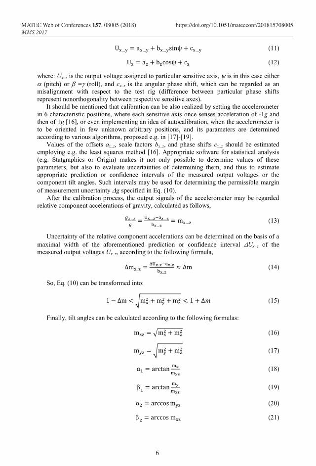
Abstract. A novel algorithm for determining pitch and roll under static or quasi-static conditions is presented. It is based on application of a triaxial micromachined accelerometer for the necessary measurements. In order to obtain a possibly high accuracy, a simple data fusion is applied. Depending on the nominal value of pitch/roll, appropriate mathematical formula is selected. Additionally, the algorithm makes it possible to check if the operating conditions are dynamic, as indications of accelerometers are then not reliable. Implementation of the algorithm makes it possible to determine pitch and roll with accuracy of ca. 0.2° over 360° or better.

Keywords: tilt, MEMS, accelerometer, algorithm, data fusion

1 Introduction Micromachined (or Micro Electromechanical Systems - MEMS) accelerometers have been applied over the last years in numerous applications and various devices [1]. Some of the devices are typical and known for a long time (e.g. automotive airbags [2]), yet other are very novel and appeared only recently (e.g. new generation of motorcycle traction control systems [3]).

Except for their crucial advantages (low cost, high reliability, compatibility with electronics, high resistance to mechanical shocks, low power consumption), their miniature size is of a big importance, especially in the case of mobile microrobots, whose control systems in many cases require information on the robot attitude. Such information is related to tilt measurement - one of the most typical application of low-g accelerometers [4].

However, it must be stated that the most limiting shortcoming of micromachined accelerometers in tilt measurements are operation only under static or quasi-static conditions as well as relatively low accuracy, as compared to their conventional counterparts. With regard to the first issue, an interesting solution is a simultaneous application of a MEMS gyroscope (or even an Inertial Measurement Unit - IMU, integrating an accelerometer, a gyroscope and optionally a magnetometer) [5]; then any operating conditions are permissible. With regard to the second issue, there is a lot of solutions of increasing the aforementioned accuracy. One of them is to apply a sensor fusion (using output signals generated by few different sensors) or a data fusion (using

* Corresponding author: [email protected] Reviewers: Milan Žmindák, Maciej Bodnicki

© The Authors, published by EDP Sciences. This is an open access article distributed under the terms of the Creative Commons Attribution License 4.0 (http://creativecommons.org/licenses/by/4.0/).

MATEC Web of Conferences 157, 08005 (2018) https://doi.org/10.1051/matecconf/201815708005MMS 2017

output signals generated by one sensor only). The presented novel algorithm for tilt measurements employs the later concept: 3 output signals of a standard triaxial MEMS accelerometer are used in a smart way in order to increase accuracy of tilt measurements as well as to simplify some mathematical transformations executed by means of a microprocessor system.

The algorithm addresses also such issues as: calibration of MEMS accelerometers and verification of the operation conditions. Besides, problems pertaining to physical alignment of MEMS accelerometers or anisotropy of triaxial MEMS accelerometers are briefly discussed.

2 Mathematical formulas Geometrical relations between components (gx, gy, gz) of the gravitational acceleration (g) and tilt angles ( - pitch, - auxiliary angle, - roll, - axial tilt [6]) are illustrated in Fig. 1. (Static or quasi-static operating conditions exclude existence of any other constant accelerations.)

Fig. 1. Components of the gravitational acceleration vs. tilt angles [1].

There are few equivalent ways of calculating the tilt angles (basically pitch and roll) on the basis of the components of the gravitational acceleration, as discussed e.g. in [1,7]. Three basic mathematical relations between the aforementioned quantities are: arc sine, arc cosine and arc tangent. Even though application of any of these equivalent formulas yields the same nominal value, each formula is characterised by different sensitivity [7].

In order to simplify the succeeding formulas, let us introduce two additional quantities, being geometric sums of the respective pairs of Cartesian components [8]:

√ (1)

√ (2)

2


output signals generated by one sensor only). The presented novel algorithm for tilt measurements employs the later concept: 3 output signals of a standard triaxial MEMS accelerometer are used in a smart way in order to increase accuracy of tilt measurements as well as to simplify some mathematical transformations executed by means of a microprocessor system.

The algorithm addresses also such issues as: calibration of MEMS accelerometers and verification of the operation conditions. Besides, problems pertaining to physical alignment of MEMS accelerometers or anisotropy of triaxial MEMS accelerometers are briefly discussed.

2 Mathematical formulas Geometrical relations between components (gx, gy, gz) of the gravitational acceleration (g) and tilt angles ( - pitch, - auxiliary angle, - roll, - axial tilt [6]) are illustrated in Fig. 1. (Static or quasi-static operating conditions exclude existence of any other constant accelerations.)

Fig. 1. Components of the gravitational acceleration vs. tilt angles [1].

There are few equivalent ways of calculating the tilt angles (basically pitch and roll) on the basis of the components of the gravitational acceleration, as discussed e.g. in [1,7]. Three basic mathematical relations between the aforementioned quantities are: arc sine, arc cosine and arc tangent. Even though application of any of these equivalent formulas yields the same nominal value, each formula is characterised by different sensitivity [7].

In order to simplify the succeeding formulas, let us introduce two additional quantities, being geometric sums of the respective pairs of Cartesian components [8]:

√ (1)

√ (2)

The proposed algorithm is based on application of arc cosine and arc tangent formulas; so, for each component tilt angle, two formulas (denoted by respective subscripts) will be employed [1,7]:

(3)

(4)

(5)

(6)

In some cases it may turn out that the auxiliary angle is more convenient for further computations. However, if the roll angle must be determined, it can be calculated directly [9]:

(7)

or on the basis of the angle [10]:

(8)

In most of measurement cases, arc tangent formulas ensure the highest sensitivity of tilt measurements [7] (thus, the highest accuracy). However, tangent is a discontinuous function at inputs of approximately ±90°. Moreover, within the vicinity of these inputs, values of the function are very high (e.g. -89.4, 89.4 for the angular domains -91°, -89° or 89°, 91°), as presented in Fig. 4. These two features are very disadvantageous, as far as microprocessor systems are concerned.

However, arc cosine function not only features continuity, but also sensitivity similar to arc tangent function [7] within the vicinity of tilt angles of ±90°. At the same time its inputs are very small (of few thousandths of V for a typical scale factor of MEMS accelerometers).

Thus, the basic idea of the proposed algorithm is to use both functions in turns. In most of the cases, arc tangent function is to be employed, except for the vicinity of tilt angles of ±90°, where arc cosine function is to be used. Then, a basic shortcoming of the latter function with regard to tilt measurements, i.e. sensitivity of zero value at tilt angles of ca. 0° [8] does not matter whatsoever.

3 Operating conditions It is well know, that indications of a triaxial accelerometer operating under static conditions must theoretically meet the following equation [11]:

√ . (9)

In the case of qausi-static conditions, output signals of the accelerometer should be first processed by means of a low-pass filter (with the cutoff frequency set e.g. to 1 Hz or lower). Then, Eq. (9) is valid; yet, in such case a decrease of accuracy of the output signals due to amplitude attenuation [12] must be taken into account.

3


Because of the existing random errors (especially accelerometer inherent noise), Eq. (9) should be replaced with the following set of inequalities:

√ , (10)

where g is the permissible margin of measurement uncertainty. At this point it must be emphasized that even though Eq. (10) is satisfied, the

accelerometer may still operate under dynamic conditions. It results from the fact that there exists an infinite group of vectors of external acceleration, disturbing tilt measurement, which added to the vector of gravitational acceleration (senses of these two kinds of vectors are opposite with respect to one another) yield a vector with an absolute value meeting conditions of Eq. (9).

The group of vectors (a1, a2, a3, ...) is illustrated in Fig. 2, where the blue circle represents all the possible positions of their tips, and the red circle represents all the possible positions of the tip of vectors (b1, b2, b3, ...), which are resultants of the gravitational acceleration and vectors (a1, a2, a3, ...).

Let us consider the simplest case, when external constant acceleration a2 acts in vertical direction, has the absolute value of 2g and the sense opposite with respect to the gravitational acceleration g. The accelerometer in this case will sense a resultant acceleration vector b2, which has the absolute value of 1g, vertical direction, yet opposite sense with respect to the gravitational acceleration g. Then, the error of measuring tilt will have the maximal possible value of 180°. The other two acceleration vectors (a1, a3) yield resultant vectors (b1, b3) having also the absolute value of 1g, yet completely inconsistent with the attitude of the accelerometer.

Fig. 2. Undetectable dynamic conditions

If no additional source of information about constant accelerations acting upon the accelerometer is available (or an information about the attitude of the accelerometer), generally, it is not possible to state if tilt measurements are correct. An exception may be a case, when it is known that the only constant external acceleration may act in a strictly defined direction. Then, on the basis of the measured Cartesian components of the resultant

4


Because of the existing random errors (especially accelerometer inherent noise), Eq. (9) should be replaced with the following set of inequalities:

√ , (10)

where g is the permissible margin of measurement uncertainty. At this point it must be emphasized that even though Eq. (10) is satisfied, the

accelerometer may still operate under dynamic conditions. It results from the fact that there exists an infinite group of vectors of external acceleration, disturbing tilt measurement, which added to the vector of gravitational acceleration (senses of these two kinds of vectors are opposite with respect to one another) yield a vector with an absolute value meeting conditions of Eq. (9).

The group of vectors (a1, a2, a3, ...) is illustrated in Fig. 2, where the blue circle represents all the possible positions of their tips, and the red circle represents all the possible positions of the tip of vectors (b1, b2, b3, ...), which are resultants of the gravitational acceleration and vectors (a1, a2, a3, ...).

Let us consider the simplest case, when external constant acceleration a2 acts in vertical direction, has the absolute value of 2g and the sense opposite with respect to the gravitational acceleration g. The accelerometer in this case will sense a resultant acceleration vector b2, which has the absolute value of 1g, vertical direction, yet opposite sense with respect to the gravitational acceleration g. Then, the error of measuring tilt will have the maximal possible value of 180°. The other two acceleration vectors (a1, a3) yield resultant vectors (b1, b3) having also the absolute value of 1g, yet completely inconsistent with the attitude of the accelerometer.

Fig. 2. Undetectable dynamic conditions

If no additional source of information about constant accelerations acting upon the accelerometer is available (or an information about the attitude of the accelerometer), generally, it is not possible to state if tilt measurements are correct. An exception may be a case, when it is known that the only constant external acceleration may act in a strictly defined direction. Then, on the basis of the measured Cartesian components of the resultant

acceleration, it possible to determine both the tilt angles as well as the external acceleration, as proposed e.g. in [13].

If it is difficult to state whether the operation conditions are static, a gyroscope can be used. MEMS gyroscopes are sometimes even integrated with MEMS accelerometers (constituting an IMU), so it is a reasonable option to use both kinds of sensors. Even though gyroscopes do not directly respond to linear acceleration, one of their shortcomings is a cross coupling error caused by linear acceleration [14]. So, if it is expected that possible constant disturbing accelerations may be of a certain value, that can be distinguished in the gyroscope noise and drift, it is an interesting and inexpensive option of verifying the operation conditions of the tilt sensor. Moreover, some constant accelerations (e.g. centripetal) are interconnected with a constant or variable rotational speed, which is a standard input of a gyroscope. So, such accelerations can be easily detected.

On the other hand, if it is certain that no constant accelerations occur, the presented considerations pertaining to the operating conditions may be ignored.

4 Calibration of MEMS accelerometers With regard to the output signal, there are two kinds of MEMS accelerometers: digital and analogue. A course of an output signal of an analogue accelerometer while tilted over a full angle (i.e. when the sensed gravitational acceleration changes within the range -1g, 1g) is presented in Fig. 3, where a is the offset and b is the scale factor. Course of a digital output signal is similar, yet the offset is approximately of a = 0.

Fig. 3. Offset and scale factor of a typical MEMS accelerometer while tilted

If a decrease of measurement accuracy is acceptable, one may assume average catalogue values for the offset and the scale factor assigned to each sensitive axis. However, if a possibly high accuracy is striven for, values of offsets and the scale factors must be determined for each sensitive axis by the way of an experimental calibration. The most accurate method of calibration is rotation of each sensitive axis of the accelerometer around a horizontal axis (the calibrated sensitive axis should be perpendicular to the rotation axis with accuracy no lower than ca. 1°). In the case of triaxial accelerometers, two sensitive axes can be calibrated at the same time (i.e. x- and z-axis while rotated around y0-axis, or y- and z-axis while rotated around x0-axis see Fig. 1), so two calibration procedures must be performed. Result of such calibration is illustrated in Fig. 3, and can be expressed by the following formula [15]:

5


(11)

(12)

where: Ux..z is the output voltage assigned to particular sensitive axis, is in this case either (pitch) or = (roll), and cx..z is the angular phase shift, which can be regarded as an misalignment with respect to the test rig (difference between particular phase shifts represent nonorthogonality between respective sensitive axes).

It should be mentioned that calibration can be also realized by setting the accelerometer in 6 characteristic positions, where each sensitive axis once senses acceleration of -1g and then of 1g [16], or even implementing an idea of autocalibration, when the accelerometer is to be oriented in few unknown arbitrary positions, and its parameters are determined according to various algorithms, proposed e.g. in [17]-[19].

Values of the offsets ax..z, scale factors bx..z, and phase shifts cx..z should be estimated employing e.g. the least squares method [16]. Appropriate software for statistical analysis (e.g. Statgraphics or Origin) makes it not only possible to determine values of these parameters, but also to evaluate uncertainties of determining them, and thus to estimate appropriate prediction or confidence intervals of the measured output voltages or the component tilt angles. Such intervals may be used for determining the permissible margin of measurement uncertainty g specified in Eq. (10).

After the calibration process, the output signals of the accelerometer may be regarded relative component accelerations of gravity, calculated as follows,

(13)

Uncertainty of the relative component accelerations can be determined on the basis of a maximal width of the aforementioned prediction or confidence interval Ux..z of the measured output voltages Ux..z, according to the following formula,

(14)

So, Eq. (10) can be transformed into:

√ (15)

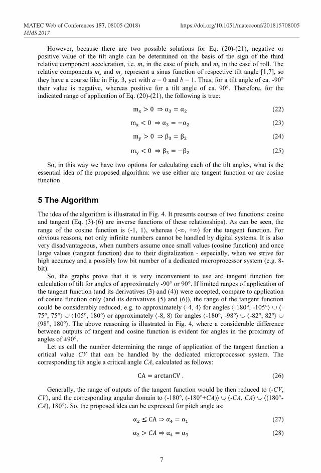
Finally, tilt angles can be calculated according to the following formulas:

√ (16)

√ (17)

(18)

(19)

(20)

(21)

6


(11)

(12)

where: Ux..z is the output voltage assigned to particular sensitive axis, is in this case either (pitch) or = (roll), and cx..z is the angular phase shift, which can be regarded as an misalignment with respect to the test rig (difference between particular phase shifts represent nonorthogonality between respective sensitive axes).

It should be mentioned that calibration can be also realized by setting the accelerometer in 6 characteristic positions, where each sensitive axis once senses acceleration of -1g and then of 1g [16], or even implementing an idea of autocalibration, when the accelerometer is to be oriented in few unknown arbitrary positions, and its parameters are determined according to various algorithms, proposed e.g. in [17]-[19].

Values of the offsets ax..z, scale factors bx..z, and phase shifts cx..z should be estimated employing e.g. the least squares method [16]. Appropriate software for statistical analysis (e.g. Statgraphics or Origin) makes it not only possible to determine values of these parameters, but also to evaluate uncertainties of determining them, and thus to estimate appropriate prediction or confidence intervals of the measured output voltages or the component tilt angles. Such intervals may be used for determining the permissible margin of measurement uncertainty g specified in Eq. (10).

After the calibration process, the output signals of the accelerometer may be regarded relative component accelerations of gravity, calculated as follows,

(13)

Uncertainty of the relative component accelerations can be determined on the basis of a maximal width of the aforementioned prediction or confidence interval Ux..z of the measured output voltages Ux..z, according to the following formula,

(14)

So, Eq. (10) can be transformed into:

√ (15)

Finally, tilt angles can be calculated according to the following formulas:

√ (16)

√ (17)

(18)

(19)

(20)

(21)

However, because there are two possible solutions for Eq. (20)-(21), negative or positive value of the tilt angle can be determined on the basis of the sign of the third relative component acceleration, i.e. mx in the case of pitch, and my in the case of roll. The relative components mx and my represent a sinus function of respective tilt angle [1,7], so they have a course like in Fig. 3, yet with a = 0 and b = 1. Thus, for a tilt angle of ca. -90 their value is negative, whereas positive for a tilt angle of ca. 90. Therefore, for the indicated range of application of Eq. (20)-(21), the following is true:

(22)

(23)

(24)

(25)

So, in this way we have two options for calculating each of the tilt angles, what is the essential idea of the proposed algorithm: we use either arc tangent function or arc cosine function.

5 The Algorithm The idea of the algorithm is illustrated in Fig. 4. It presents courses of two functions: cosine and tangent (Eq. (3)-(6) are inverse functions of these relationships). As can be seen, the range of the cosine function is -1, 1, whereas -, + for the tangent function. For obvious reasons, not only infinite numbers cannot be handled by digital systems. It is also very disadvantageous, when numbers assume once small values (cosine function) and once large values (tangent function) due to their digitalization - especially, when we strive for high accuracy and a possibly low bit number of a dedicated microprocessor system (e.g. 8-bit).

So, the graphs prove that it is very inconvenient to use arc tangent function for calculation of tilt for angles of approximately -90° or 90°. If limited ranges of application of the tangent function (and its derivatives (3) and (4)) were accepted, compare to application of cosine function only (and its derivatives (5) and (6)), the range of the tangent function could be considerably reduced, e.g. to approximately -4, 4 for angles -180°, -105° -75°, 75° 105°, 180° or approximately -8, 8 for angles -180°, -98° -82°, 82° 98°, 180°. The above reasoning is illustrated in Fig. 4, where a considerable difference between outputs of tangent and cosine function is evident for angles in the proximity of angles of ±90°.

Let us call the number determining the range of application of the tangent function a critical value CV that can be handled by the dedicated microprocessor system. The corresponding tilt angle a critical angle CA, calculated as follows:

. (26)

Generally, the range of outputs of the tangent function would be then reduced to -CV, CV, and the corresponding angular domain to -180°, (-180°+CA) -CA, CA (180°-CA), 180°. So, the proposed idea can be expressed for pitch angle as:

(27)

(28)

7


and for roll angle as:

(29)

(30)

Fig. 4. Angular regions of data fusion

A problem similar to application of Eq. (20) or (21) is related to measurements over the full angular range of -180°, 180° while using Eq. (18) or (19). It must be distinguished whether the calculated tilt angle is contained within a sub-range of -90°, 90° or the remaining sub-range of -180°, 90°) (90°, 180°. This time, the sign of the mz relative component acceleration is decisive. If it has a positive value (see the red part of the cos(x) course in Fig. 4), the tilt angle is contained within the first sub-range, whereas its negative value indicates the second sub-range (see the blue part of the cos(x) course in Fig. 4).

So, formulas valid for the pitch angle are the following [20]:

(31)

If Eq. (22) is true, then:

(32)

otherwise Eq. (23) is true, so:

(33)

Analogical formulas are valid for the roll angle:

(34)


(35)


(36)

8


and for roll angle as:

(29)

(30)

Fig. 4. Angular regions of data fusion

A problem similar to application of Eq. (20) or (21) is related to measurements over the full angular range of -180°, 180° while using Eq. (18) or (19). It must be distinguished whether the calculated tilt angle is contained within a sub-range of -90°, 90° or the remaining sub-range of -180°, 90°) (90°, 180°. This time, the sign of the mz relative component acceleration is decisive. If it has a positive value (see the red part of the cos(x) course in Fig. 4), the tilt angle is contained within the first sub-range, whereas its negative value indicates the second sub-range (see the blue part of the cos(x) course in Fig. 4).

So, formulas valid for the pitch angle are the following [20]:

(31)


(32)


(33)

Analogical formulas are valid for the roll angle:

(34)


(35)


(36)

To summarise, the presented algorithm consists of the following steps: 1. Assume the maximal value of parameter CV 2. Compute value of the critical angle CA according to (26) 3. Calibrate the accelerometer in order to estimate: ax, ay, az, bx, by, bz, Ux, Uy, Uz 4. Compute the permissible margin of the relative acceleration m according to (14) 5. Set an unknown orientation of the accelerometer to be determined 6. Record the output signals of the accelerometer: Ux, Uy, Uz 7. Compute the relative component accelerations mx, my, mz according to (13) 8. Verify condition (15); if not satisfied get back to step 6 9. Compute the resultant accelerations mxz, myz according to (16)-(17) 10. Determine value of pitch and roll according to (20) and (21) 11. If condition (28) is satisfied, proceed to step 16 12. Determine value of pitch according to (18) 13. Condition (27) is satisfied 14. Determine the final value of pitch according to (31)-(33) 15. Proceed to step 17 16. Determine the final value of pitch according to (22) or (23) 17. Final value of pitch has been determined 18. If condition (30) is satisfied, proceed to step 23 19. Determine value of roll according to (19) 20. Condition (29) is satisfied 21. Determine the final value of roll according to (34)-(36) 22. Proceed to step 24 23. Determine the final value of roll according to (24) or (25) 24. Final value of roll has been determined

6 Experimental verification In order to evaluate accuracy of tilt measurements according to the proposed algorithm, few experiments were performed, using a computer-controlled test rig minutely described in [21]. Low-g triaxial MEMS accelerometers by Analog Devices Inc. were tested.

The error was calculated as an absolute value of a difference between the real tilt angle (applied by means of the test rig) and the estimated tilt angle (calculated on the basis of the average value related to output signals of the tested accelerometer, using the calibration parameters defined in Eq. (11) and (12), which had been determined beforehand). It was accepted that the arc cosine formula was used within the range of -105°, -75° 75°, 105°, and the arc tangent formula within the remaining range.

a) b)

Fig. 5. Error of deterring component tilt angle

9


The obtained results prove that the presented algorithm makes it possible to obtain errors typical for application of arc tangent formula (in other words, almost at constant measurement sensitivity - in contrary to application of arc cosine formula - see Fig. 5a), yet without using this function within the angular regions where its outputs are very large. Fig. 5b proves that application of arc cosine formula within the range of 75°, 105°, does not result in increasing the measurement error. The presented course is of a random character.

The experimental studies have proven correctness of the proposed algorithm. A relatively high accuracy has been obtained: better than 0.2 over the full angular range, so similar to the value reported in [20], when an algorithm was used, which employed only arctangent formula.

Conclusions

The proposed algorithm makes it possible to determine pitch and roll within the full angular range with accuracy of ca. 0.2 degrees arc. It makes it possible to employ a simple microprocessor system for the necessary computations.

Using accurate low-range MEMS accelerometers, called MEMS inclinometers [22], [23], the accuracy of tilt measurements may be considerably increased, at least to 0.1 degrees arc [23]. Yet, since the inclinometers are single- or dual-axis accelerometers, in order to implement the proposed algorithm, at least two inclinometers must be applied, without neglecting the problem of aligning their sensitive axes.

Even higher accuracies are reported while applying differential MEMS accelerometers [24]. More detailed information regarding application of MEMS accelerometers for tilt measurements (e.g. selecting their types, configurations, spatial arrangements and imperfections) can be found in [1]. It must not be neglected that alignment of the sensitive axes of MEMS accelerometers is a problem important especially in tilt measurements, as proved in [25], [26].

References 1. S. Łuczak, R. Grepl, M. Bodnicki, Selection of MEMS Accelerometers for Tilt

Measurements. J. Sensors 2017, Article ID 9796146 (2017) 2. M. Jrad, M.I. Younis, F. Najar, Modeling and Design of an Electrically Actuated

Resonant Switch. MATEC Web of Conf. 1, Article No. 04001 (2012) 3. S. Łuczak, Tilt Measurements in BMW Motorcycles, in R. Jabłoński, R. Szewczyk

(Eds.), Recent Global Research and Education: Technological Challenges. (Springer International Publishing, Cham, Switzerland, 2017)

4. J. S. Wilson, Sensor Technology Handbook. (Newnes, Burlington, 2005) 5. L. Beran, P. Chmelar, L. Rejfe, An Increase in Estimation Accuracy Position

Determination of Inertial Measurement Units. MATEC Web of Conf. 75, Article No. 05001 (2016)

6. S. Łuczak, Specific Measurements of Tilt with MEMS Accelerometers, in R. Jabłoński, T. Brezina (Eds.), Mechatronics. Recent Technological and Scientific Advances. (Springer-Verlag, Berlin Heidelberg, 2012)

7. S. Łuczak, Guidelines for Tilt Measurements Realized by MEMS Accelerometers. Int. J. Precis. Eng. Manuf. 15, 2012-2019 (2014)

8. S. Łuczak, W. Oleksiuk, M. Bodnicki, Sensing Tilt With MEMS Accelerometers. IEEE Sensors J. 6, 1669-1675 (2006)

10


The obtained results prove that the presented algorithm makes it possible to obtain errors typical for application of arc tangent formula (in other words, almost at constant measurement sensitivity - in contrary to application of arc cosine formula - see Fig. 5a), yet without using this function within the angular regions where its outputs are very large. Fig. 5b proves that application of arc cosine formula within the range of 75°, 105°, does not result in increasing the measurement error. The presented course is of a random character.

The experimental studies have proven correctness of the proposed algorithm. A relatively high accuracy has been obtained: better than 0.2 over the full angular range, so similar to the value reported in [20], when an algorithm was used, which employed only arctangent formula.

Conclusions

The proposed algorithm makes it possible to determine pitch and roll within the full angular range with accuracy of ca. 0.2 degrees arc. It makes it possible to employ a simple microprocessor system for the necessary computations.

Using accurate low-range MEMS accelerometers, called MEMS inclinometers [22], [23], the accuracy of tilt measurements may be considerably increased, at least to 0.1 degrees arc [23]. Yet, since the inclinometers are single- or dual-axis accelerometers, in order to implement the proposed algorithm, at least two inclinometers must be applied, without neglecting the problem of aligning their sensitive axes.

Even higher accuracies are reported while applying differential MEMS accelerometers [24]. More detailed information regarding application of MEMS accelerometers for tilt measurements (e.g. selecting their types, configurations, spatial arrangements and imperfections) can be found in [1]. It must not be neglected that alignment of the sensitive axes of MEMS accelerometers is a problem important especially in tilt measurements, as proved in [25], [26].

References 1. S. Łuczak, R. Grepl, M. Bodnicki, Selection of MEMS Accelerometers for Tilt

Measurements. J. Sensors 2017, Article ID 9796146 (2017) 2. M. Jrad, M.I. Younis, F. Najar, Modeling and Design of an Electrically Actuated

Resonant Switch. MATEC Web of Conf. 1, Article No. 04001 (2012) 3. S. Łuczak, Tilt Measurements in BMW Motorcycles, in R. Jabłoński, R. Szewczyk

(Eds.), Recent Global Research and Education: Technological Challenges. (Springer International Publishing, Cham, Switzerland, 2017)

4. J. S. Wilson, Sensor Technology Handbook. (Newnes, Burlington, 2005) 5. L. Beran, P. Chmelar, L. Rejfe, An Increase in Estimation Accuracy Position

Determination of Inertial Measurement Units. MATEC Web of Conf. 75, Article No. 05001 (2016)

6. S. Łuczak, Specific Measurements of Tilt with MEMS Accelerometers, in R. Jabłoński, T. Brezina (Eds.), Mechatronics. Recent Technological and Scientific Advances. (Springer-Verlag, Berlin Heidelberg, 2012)

7. S. Łuczak, Guidelines for Tilt Measurements Realized by MEMS Accelerometers. Int. J. Precis. Eng. Manuf. 15, 2012-2019 (2014)

8. S. Łuczak, W. Oleksiuk, M. Bodnicki, Sensing Tilt With MEMS Accelerometers. IEEE Sensors J. 6, 1669-1675 (2006)

9. D. Jurman, M. Jankovec, R. Kamnik, M. Topič, Calibration and data fusion solution for the miniature attitude and heading reference system. Sens. Actuators A: Phys. 138, 411-420 (2007)

10. S. Popowski, Determination of Pitch and Roll Angles in Low Cost Land Navigation Systems. J. Aeronautica Integra 1, 93-97 (2008) (in Polish)

11. J.C. Lötters, J. Schipper, P.H. Veltink, W. Olthuis, P. Bergveld, Procedure for in-use calibration of triaxial accelerometers in medical applications, Sens. Actuators A: Phys. 68, 221-228 (1998)

12. A. Albarbar, A. Badri, J. K. Sinha, A. Starr, Performance evaluation of MEMS accelerometers. Measurement 42, 790-795 (2009)

13. R. Dao, Inclination Sensing of Moving Vehicle. Application Note n/r 3/12/03, MEMSIC Inc. (2003)

14. S. Liu, R. Zhu, Micromachined Fluid Inertial Sensors, Sens. 17, 367 (2017) 15. S. Łuczak, Experimental Studies of Hysteresis in MEMS Accelerometers:

A Commentary. IEEE Sensors J. 15, 3492-3499 (2015) 16. S. Stančin, S. Tomažič, Time- and Computation-Efficient Calibration of MEMS 3D

Accelerometers and Gyroscopes. Sens. 14, 14885-14915 (2014) 17. I. Frosio, F. Pedersini, N. A. Borghese, Autocalibration of Triaxial MEMS

Accelerometers With Automatic Sensor Model Selection. IEEE Sensors J. 12, 2100-2108 (2012)

18. M. Sipos, P. Paces, J. Rohac, P. Novacek, Analyses of triaxial accelerometer calibration algorithms. IEEE Sensors J. 12, 1157-1165 (2012)

19. W. Yang, B. Fang, Y. Y. Tang, J. Qian, X. Qin, W. Yao, A robust inclinometer system with accurate calibration of tilt and azimuth angles. IEEE Sensors J. 13, 2313-2321 (2013)

20. S. Łuczak, Advanced Algorithm for Measuring Tilt with MEMS Accelerometers, in R. Jabłoński, M. Turkowski, R. Szewczyk (Eds.), Recent Advances in Mechatronics. (Springer-Verlag, Berlin Heidelberg, 2007)

21. S. Łuczak, Dual-Axis Test Rig for MEMS Tilt Sensors. Metrol. Meas. Syst. 21, 351-362 (2014)

22. TS1000T Colybris Acceleration Inclinometer. Preliminary Datasheet, Safran Colibrys SA

23. The SCA103T differential inclinometer series, Datasheet, Murata Electronics Oy 24. S. Zhao, Y. Li, E. Zhang, P. Huang, H. Wei, Differential amplified high-resolution tilt

angle measurement system. Rev. Scientific Instrum. 85, 096104 (2014) 25. S. Łuczak, Fast Alignment Procedure for MEMS Accelerometers. R. Jabłoński, T.

Brezina (Eds.), Advanced Mechatronics Solutions. (Springer International Publishing, Cham, Switzerland, 2016)

26. S. Łuczak, Effects of Misalignments of MEMS Accelerometers in Tilt Measurements. T. Brezina, R. Jabloński (Eds.), Mechatronics 2013. Recent Technological and Scientific Advances. (Springer International Publishing, Cham, Switzerland, 2014)

11


Novel algorithm for tilt measurements using MEMS ...

Documents

Transcript of Novel algorithm for tilt measurements using MEMS ...