Florida State University Libraries

Electronic Theses, Treatises and Dissertations The Graduate School

2004

Magnetic MEMS and Its ApplicationsPan Zheng

Follow this and additional works at the FSU Digital Library. For more information, please contact lib-ir@fsu.edu

THE FLORIDA STATE UNIVERSITY

COLLEGE OF ENGINEERING

MAGNETIC MEMS AND ITS APPLICATIONS

By

PAN ZHENG

A Dissertation submitted to the Department of Mechanical Engineering

in partial fulfillment of the requirements for the degree of

Doctor of Philosophy

Degree Awarded: Summer Semester, 2004

ii

The members of the Committee approve the dissertation of Pan Zheng defended on July 6, 2004.

Ching-Jen Chen

Professor Co-Directing Dissertation

Yousef Haik Professor Co-Directing Dissertation Jim P. Zheng Outside Committee Member Namas Chandra Committee Member Peter Kalu Committee Member

Approved: Chiang Shih, Chair, Department of Mechanical Engineering

Ching-Jen Chen, Dean, College of Engineering

The Office of Graduate Studies has verified and approved the above named committee members.

iii

To My Parents

iv

ACKNOWLEDGEMENTS

I would like to express my gratitude to my advisors Dr. Ching-Jen Chen and Dr. Yousef

Haik, for their support, patience, and encouragement throughout my graduate studies.

Dr. Chen has not only provided the research advice that was essential to the completion

of this dissertation but also has inspired me with his broad and insightful visions on the

academic field and his optimism and enthusiasm towards life. Without his valuable

encouragement and suggestions, this work would not have been possible.

Dr. Haik has considerably helped me to accomplish the work with his perceptive outlook

of engineering, critical reviews and suggestions on my research project. His hardworking

attitude and creative ideas in research motivate me to pursue success in my research.

Thanks to Dr. Jim P. Zheng of the Department of Electrical and Computer Engineering

for allowing me to use his Pulsed Laser Deposition Apparatus and serving on my

dissertation committee. Thanks to Dr. Eric Lochner and Mr. Ian Winger of the FSU

Center for Material Research and Technology (MARTECH) for using their facilities.

I appreciate Dr. Namas Chandra and Dr. Peter Kalu for serving on my dissertation

committee.

I also like to extend my thanks to my colleagues and friends of the Center for

Nanomagnetics and Biotechnology. Their valuable discussions and suggestions have

broadened my interdisciplinary knowledge.

Lastly, I also deeply thank my parents for their faithful support and confidence in my

ability to complete this work.

v

TABLE OF CONTENTS List of Tables……………………………………………………………………………viii List of Figures ……………………………………………………………………………ix Abstract …………………………………………………………………………….……xii

CHAPTER 1

INTRODUCTION ...........................................................................................1

1.1 Objective of the Research ......................................................................................... 1 1.2 Historical Development of Micro Devices ............................................................... 1 1.3 Method of Actuation in MEMS ................................................................................ 3

1.3.1 Electrostatic Actuation....................................................................................... 3 1.3.2 Thermal Actuation ............................................................................................. 5 1.3.3 Shape Memory Alloy (SMA) Actuation............................................................ 7 1.3.4 Piezoelectric Actuation ...................................................................................... 7 1.3.5 Magnetic Actuation............................................................................................ 8

1.4 Motivation of Research........................................................................................... 11 1.5 Outline of the Dissertation ...................................................................................... 13

CHAPTER 2

MAGNETIC FILM DEPOSITION FOR MEMS .........................................14

2.1 General Remarks..................................................................................................... 14 2.2 Methods of Material Deposition ............................................................................. 15

2.2.1 Chemical Vapor Deposition............................................................................. 16 2.2.2 Evaporation and Sputtering.............................................................................. 18 2.2.3 Pulsed Laser Deposition .................................................................................. 18

2.3 Magnetic Material And Its Properties..................................................................... 21 2.3.1 Magnetic Units................................................................................................. 21 2.3.2 Magnetic Material............................................................................................ 23

2.4 Deposition of NdFeB Film...................................................................................... 27 2.4.1 Review of the Study of NdFeB film ................................................................ 27 2.4.2 Experiment Setting Up..................................................................................... 28 2.4.3 Measurement Methods..................................................................................... 32

2.5 Discussion of Film Magnetic Properties................................................................. 35 2.5.1 External Magnetic Effect On Film Magnetic Properties ................................. 35 2.5.2 Temperature Effect On Film’s Magnetic Properties........................................ 39

2.6 Summary ................................................................................................................. 41

vi

CHAPTER 3

MATHEMATICL PRINCIPLES AND SIMULATIONS

OF MAGNETIC COUPLING.......................................................................42

3.1 Magnetic Field Calculation..................................................................................... 42 3.2 Magnetic Coupling Force and Torque .................................................................... 45 3.3 Magnetic Force on Magnetic Particles ................................................................... 51 3.4 Numerical Element Method for Magnetic Field..................................................... 54 3.5 Numerical Simulations of Magnetic Coupling ....................................................... 57

3.5.1 Simulations Arrangements and Goals.............................................................. 57 3.5.2 Effecting Parameters for the Magnetic Coupling ............................................ 61 3.5.3 Conclusion of Simulations............................................................................... 70

3.6 Summary ................................................................................................................. 70

CHAPTER 4

MAGNETICALLY DRIVEN MINI SCREW PUMP ..................................71

4.1 Introduction of Screw Pump ................................................................................... 71 4.2 Magnetically Driven Screw Pumps Performance ................................................... 74

4.2.1 Two Different Mini Screw Pump Prototypes .................................................. 74 4.2.2 Experiment Procedures .................................................................................... 76 4.2.3 Experimental Results ....................................................................................... 77

4.3 Summary ................................................................................................................. 79

CHAPTER 5

MAGNETIC DRIVEN MICRO VISCOUS SPIRAL PUMP.......................80

5.1 Introduction............................................................................................................. 80 5.2 Magnetically Driven Pumps ................................................................................... 81 5.3 Microfabrication and Magnetic Deposition ............................................................ 83

5.3.1 Microfabrication and SUMMiT....................................................................... 84 5.3.2 Magnetic Material Deposition ......................................................................... 88 5.3.3 Two New Designs of Microgears for Film Deposition ................................... 90

5.4 Magnetic Micro Spiral Pump.................................................................................. 94 5.4.1 Introduction of Viscous Drag Spiral Pump...................................................... 94 5.4.2 Fabrication of Magnetic Micro Spiral Pump ................................................... 96

5.5 Magnetic Coupling Force and Torque of Micro Spiral Pump ................................ 98 5.6 Summary ............................................................................................................... 103

vii

CHAPTER 6

EXPERIMENTS OF SCALED UP MODELS OF MICROPUMP........... 104

6.1 Two Scaled-up Models for Micro Spiral Pumps .................................................. 104 6.2 Experimental Set-up.............................................................................................. 109 6.3 Experimental Results and Discussing................................................................... 111 6.4 Summary ............................................................................................................... 115

CHAPTER 7

NUMERICAL SIMULATION OF SCALED UP MODELS OF MICROPUMP ............................................................................................ 117

7.1 Introduction........................................................................................................... 117 7.2 Characteristics of Fluid Flow in Micro-scale Device ........................................... 118 7.3 Formulation of Problems ...................................................................................... 120

7.3.1 Governing Equations ..................................................................................... 120 7.3.2 Boundary Conditions for Governing Equations ............................................ 121

7.4 Numerical Simulation ........................................................................................... 125 7.4.1 Numerical Simulation of rotating spiral model ............................................. 125 7.4.2 Numerical Simulation of fixed spiral model.................................................. 130

7.5 Discussion of Numerical Simulation Results ....................................................... 133 7.6 Summary ............................................................................................................... 138

CHAPTER 8

CONCLUSIONS AND RECOMMENDATIONS..................................... 140

8.1 Summary of Magnetic-MEMS Research.............................................................. 140 8.1.1 Magnetic Material Deposition and Magnetic Coupling................................. 140 8.1.2 Magnetic MEMS and Micropumps ............................................................... 142

8.2 Future Prospects of the Relative Research............................................................ 144

REFERENCES ........................................................................................... 146

BIOGRAPHICAL SKETCH……………………………………………...155

viii

LIST OF TABLES

Table 1.1 W (J/m3) for Several Low Voltage Microactuators [27, 28] ............................ 10

Table 2.1 The Rrelationship Between Some Magnetic Parameters in cgs and S.I. Units 25 Table 2.2 Summary of Different Types of Magnetic Behavior ....................................... 25 Table 3.1 Summary of the Boundary Value Problems for Magnetostatics ...................... 55 Table 3.2 Verification of the Ampere Package................................................................. 59 Table 7.1 Knudson Number Regimes............................................................................. 119 Table 7.2 Boundary Conditions of Fixed-spiral Channel ............................................... 122 Table 7.3 Boundary Conditions of Rotating Spiral Channel .......................................... 122 Table 7.4 Spiral Geometry Parameters in Micro Pump Design...................................... 137

ix

LIST OF FIGURES Figure 1.1 Electrostatic Working Principle [12]................................................................. 4 Figure 1.2 (a): Comb Driver (Left) .................................................................................... 4 Figure 1.2 (b): Torsional Ratchet Actuator (TRA) (Right) [13]......................................... 4 Figure 1.3. Schematic Diagram of Micropump [14]........................................................... 5 Figure 1.4 Micromachined Thermal Actuator .................................................................... 6 Figure 1.5 Thermally Actuated Microvalve [16,17]........................................................... 7 Figure 1.6 SEM of Electromagnetic Core [25,26].............................................................. 9 Figure 1.7 Micromachined Toroidal Inductor [25,26]........................................................ 9 Figure 1.8 Magnetic Levitator .......................................................................................... 10 Figure 2.1 CVD Horizontal Reactor ................................................................................. 16 Figure 2.2 Evaporation Systems [38]................................................................................ 17 Figure 2.3 Sputtering Systems [38] ................................................................................. 17 Figure 2.4 Schematic Diagram of Pulsed Laser Deposition ............................................. 18 Figure 2.5 Pulsed Laser Deposition Apparatus................................................................. 20 Figure 2.6 (a) A Typical M versus H Hysteresis Curve. .................................................. 24 Figure 2.6 (b) The Corresponding B versus H.................................................................. 24 Figure 2.7 Soft and Hard Magnetic Properties. ................................................................ 24 Figure 2.8 B-H curve of Grade 30 Nd2Fe14B Compound................................................. 29 Figure 2.9 PLD Plume of Energetic Species of the Target Material ................................ 29 Figure 2.10 Illustration of the Experiment Setup.............................................................. 30 Figure 2.11 External Magnetic Field Distributions in the Substrate ................................ 31 Figure 2.12 The Thickness and Roughness of Film on Silicon Substrate ........................ 32 Figure 2.13 SEM and AFM of Film Surface .................................................................... 33 Figure 2.14 XRD Pattern of Target Nd2Fe14B.................................................................. 34

Figure 2.15 XRD Patterns of Film Deposited at 250°C ................................................... 35 Figure 2.16 Magnetization Hysteresis in the Perpendicular Direction with and without

External Fields .......................................................................................................... 36

Figure 2.17 XRD Patterns of Film Deposited at 500°C, 550°C ....................................... 37 Figure 2.18 Magnetization Hysteresis Loops In and Perpendicular to the Film Deposited

at 500°C. ................................................................................................................... 39 Figure 2.19 Magnetization Hysteresis Loop In and Perpendicular to the Film Deposited at

650°C. ....................................................................................................................... 40

Figure 2.20 XRD Pattern of the Film Deposited at 650°C ............................................... 40 Figure 3.1 Coordination of Permanent Magnet in the Problem........................................ 44 Figure 3.2 Superparamagnetic Hysteresis........................................................................ 52 Figure 3.3 Magnetically Driven Mini-screw Pump .......................................................... 57 Figure 3.4 Two Repulsive Magnets .................................................................................. 58 Figure 3.5 2-pole Magnetic Coupling............................................................................... 60 Figure 3.6 4-pole Magnetic Coupling............................................................................... 60 Figure 3.7 6-pole Magnetic Coupling............................................................................... 60

x

Figure 3.8 Magnetic Induction Distributions on the plane that is 0.5mm above the Load Magnets of 2-pole Set (a) Solid-contour (b) 3-D Profile ......................................... 62

Figure 3.9 The Magnetic Induction Distributions on the Plane that is 0.5mm above the Load Magnets of 4-pole set (a) Solid-contour (b) 3-D Profile ................................. 63

Figure 3.10 The Magnetic Induction Distribution on the Plane that is 0.5mm above the Load Magnets of 6-pole set (a) Solid-contour (b) 3-D Profile ................................. 64

Figure 3.11 B-field of 2,4,6-pole Magnetic Coupling with Separation of 30mm the Poles................................................................................................................................... 65

Figure 3.12 B-field of 2,4,6-pole Magnetic Coupling with Separation of 4mm .............. 65 Figure 3.13 Magnetic Force of Different Coupling Poles ................................................ 66 Figure 3.14 Magnetic Force versus Separation................................................................. 67 Figure 3.15 Magnetic Torque versus Separation .............................................................. 68 Figure 3.16 Torque of 2,4,6-pole Magnetic Coupling with Separation of 4mm at Different

Rotation Angle θ ....................................................................................................... 69 Figure 4.1 Schematic Diagram of a Magnetically Driven Screw Pump........................... 73 Figure 4.2 Model M1: Lateral Flow Configuration .......................................................... 75 Figure 4.3 Model M2: Combined Flow Configuration..................................................... 75 Figure 4.4 Experimental Setting of Magnetic Driven Screw Pump ................................. 76 Figure 4.4 Model 1 Pump Characteristics......................................................................... 77 Figure 4.5 Model 2 Pump Characteristics......................................................................... 78 Figure 5.1 Spiral Pump Driven by Electrostatic Comb Driver......................................... 81 Figure 5.2 Micro Spiral Pump Driven by TRA ............................................................... 82 Figure 5.3 Magnetically Driven Spiral Pump................................................................... 83 Figure 5.4 SUMMiT-5 Layer Description ........................................................................ 85 Figure 5.5 Standard Release Processes............................................................................. 87 Figure 5.6 (a) Before Deposition (b) Pattern Transfer by Mask (c, d) Gear Surface After

Deposition ................................................................................................................. 89 Figure 5.7 Illustration of the PLD Setting-up for Microgear............................................ 90 Figure 5.8 Released Holes in the Microgear Surface ....................................................... 90 Figure 5.9 New Design of the Gear with Releasing (etching) Holes Through the Substrate

................................................................................................................................... 92 Figure 5.10 A-A Cross-section View of the Dack Releasing ........................................... 92 Figure 5.11 Center Rectangle Release Cut of Microgear ................................................. 93 Figure 5.12 A-A Cross-section View of Rectangle Release Cut ...................................... 94 Figure 5.13 Schematic Illustration of Spiral Pump.......................................................... 96 Figure 5.14 A Cross Section Through the Spiral Disk Centerline.................................... 97 Figure 5.15 The Hysteresis Loop of Perpendicular Magnetization of NdFeB Film......... 98 Figure 5.16 The Normal Magnetic Induction Distribution on the Films Without Angular

Offset between the Driving Magnets and Driven Microgear.................................. 100 Figure 5.17 The Normal Magnetic Induction Distribution on the Films with 45 Degrees

Angular Offset between Driving Magnets and Driven Microgear ......................... 100 Figure 5.18 The Normal Magnetic Induction Distribution on the Films with 90 Degrees

Angular Offset between Driving Magnets and Driven Microgear ......................... 101 Figure 5.19 The Relation of the Magnetic Force and Angular Offset ............................ 101

xi

Figure 5.10 The Relation of the Magnetic Torque and Angular Offset.......................... 102 Figure 6.1 Scaled-up Pump for Rotating Spiral Disk Design......................................... 106 Figure 6.2 (a) Experimental Mounting of the Rotating Spiral Pump ............................. 107 Figure 6.2 (b) The Magnetic Coupling between the Motor and Pump........................... 107 Figure 6.3 The Perspective Drawing of the Rotating Part of Scaled-up Spiral Pump

Design ..................................................................................................................... 108 Figure 6.4 Scaled-up Pump Model for Fixed Spiral Design........................................... 109 Figure 6.5 Experimental Set up for Scaled-up Pump Model .......................................... 110 Figure 6.6 Rotation Direction of the Spiral Channel ...................................................... 111

Figure 6.7 Flow Rate versus Head Pressure of 2π Angular Span with the 0.1 mmGap. 112

Figure 6.8 Flow Rate versus Head Pressure of 2π Angular Span with the 0.4 mmGap. 112

Figure 6.9 Flow Rate versus Head Pressure of 8π Angular Span with the 0.1 mmGap. 113

Figure 6.10 Flow Rate versus Head Pressure of 8π Angular with the 0.4 mm Gap....... 114 Figure 6.11 The Highest Head Pressure the Pump Can Overcome (flow rate is 0 at this

point) with Counterclockwise Rotation Direction .................................................. 115 Figure 7.1 Outline of the Spiral Channel ........................................................................ 121 Figure 7.2 Illustration of the Inlet Situation of Experiment............................................ 123 Figure 7.3 3-D View of the Numerical Simulation Model ............................................. 125 Figure 7.4 Flow Grids of the Simulation Model............................................................. 126 Figure 7.5 Numerical Simulated Mass Flow Rates versus Different Spiral Rotation Speed

................................................................................................................................. 127 Figure 7.6 Velocity Contour on the Top of the Rotating Spiral Channel @1800 rpm... 129 Figure 7.7 Velocity Contour on the Bottom of the Rotating Spiral @1800 rpm............ 129 Figure 7.8 Velocity Contour in Rotating Spiral Channel Cross Section @1800 rpm .... 129 Figure 7.9 Pressure Distributions on the Middle of the Rotating Channel @1800 rpm. 130 Figure 7.10 Numerical Simulated Mass Flow Rates versus Different Top Disk Rotation

Speed....................................................................................................................... 131 Figure 7.11 Velocity Contour on the Top of the Spiral Channel @1800 rpm................ 132 Figure 7.12 Velocity Contour on the Plane 5% Below the Top Disk @1800 rpm......... 132 Figure 7.13 Velocity Contour in Fixed Spiral Channel Cross Section @1800 rpm....... 132 Figure 7.14 Pressure Distribution Below the Top Disk @1800 rpm.............................. 133 Figure 7.16 Outlet Position 1 of Rotating Spiral ............................................................ 134 Figure 7.17 Outlet Position 2 of Rotating Spiral ............................................................ 134

xii

ABSTRACT

This research is to investigate the performance of mini and micro devices driven

magnetically through simulations and experiments. Micro-Electro-Mechanical Systems

(MEMS) invoking magnetic coupling were designed and tested. Scaled up models and

numerical simulation of the micro spiral channel flow were also presented.

Magnetic devices can generate larger forces for larger distance than their

electrostatic counterparts; the energy density between the magnetic plates is usually

larger than that between the electric plates. Properly designed, magnetic actuators can be

made to hold high torques with no intervening wires. Magnetic actuation may be

considered a feasible method to drive the MEMS with advantages.

Pulsed laser deposition method is used for growing magnetic material to the

surface of micro device. Magnetic material properties are investigated. A permanent

magnet made of NdFeB is used as a target for pulsed laser deposition to produce the thin

film on a micro device which may induce magnetic coupling with external magnet

sources. The properties of the thin film formed at different substrate temperatures and

effects of external magnetic field to the thin magnetic film are presented.

A mini screw pump invoking the magnetic driven system is demonstrated and its

working performance is verified experimentally. The experiment on mini screw pump is

to demonstrate the advantages of magnetic coupling and to verify the feasibility of

magnetic coupling concept in a real device. The mathematical modeling and numerical

simulations for magnetic coupling are also carried out.

Further, the design and microfabrication technologies are introduced for a

magnetically driven micro gear and micro viscous pump. Through the study of several

experiments, improvements for designs are made.

Due to the challenge in testing the actual microdevices, scaled-up experiments for

magnetically driven viscous pumps are made. These studies simulate the performance of

the micro size counterpart. In addition, the analyses of flow in micro size channels are

xiii

made. Boundary conditions required for a proper simulation are discussed. Numerical

simulations required for a pump performance are given. The factors to affect the pump

performance are discussed based on the theoretical model, experiment and numerical

simulation results.

CHAPTER 1

INTRODUCTION

1.1 Objective of the Research

The present research is to investigate the performance of mini and micro devices.

The focus is on actuation of Micro-Electro-Mechanical Systems (MEMS) invoking

magnetic coupling between the micro device and the driving mechanism.

The objectives of this study are (1) to investigate the fundamentals of magnetic

driven system and its application to mini screw pump and micro spiral pump; (2) to

develop mathematical models and simulation for the magnetic couplings; (3) to

demonstrate the characteristics of the micro magnetic device; (4) to investigate the

method of deposition of magnetic materials to the micro devices; (5) to fabricate

magnetically driven micro gear system and (6) to conduct experiments in scaled up

magnetic driven viscous pumps that simulate the performance of the micro size

counterpart and to carry out the relative fluid analysis for macro and micro size channels .

1.2 Historical Development of Micro Devices

Nobel laureate physicist Richard P. Feynman in his 1961 lecture on

electromechanical miniaturization entitled “There is Plenty of Room at the Bottom” said :

“Small but movable machines may or may not be useful, but they surely would be fun to

1

2

make,” and, 23 years later, in his 1983 presentation “Infinitesimal Machinery”[1,2],

Feynman still said “There is no use for these machines, so I still don’t understand why I

am fascinated by the question of making small machines with movable and controllable

parts.”. However, in the past decades, those very small machines began to find increased

applications in a variety of industrial and medical fields. By the year of 2004, there was

estimated $82 billion in revenues for the microsystems and related products [3].

Accelerometers for automobile airbags [4], keyless entry systems, dense arrays of

micromirrors for high-definition optical displays [5], scanning electron microscope tips to

image single atoms, micro-heat-exchangers for cooling of electronic circuits, reactors for

separating biological cells, blood analyzers and pressure sensors for catheter tips are a

few in current use. In addition, microducts are used in infrared detectors, diode lasers,

miniature gas chromatographs and highfrequency fluidic control systems. Micropumps

are used for ink-jet printing, environmental testing and electronic cooling [6]. Potential

medical applications for small pumps include controlled delivery and monitoring of

minute amounts of medication or analysis of chemicals, and development of monitor for

diabetic patients [103, 104].

The research about those small machines was finally developed as an

interdisciplinary engineering field: Micro-Electro-Mechanical Systems (MEMS). It is

hard to make a unanimous definition about MEMS. Basically, MEMS are machines or

devices that integrate the micron size mechanical and electrical components to achieve

certain engineering function by electromechanical or electrochemical means of the

sensing, actuating, signal processing elements [7,8,9].

In the past decades, the successful applications of MEMS in many industries and

people’s common living stimulate the further relative research in material, packaging and

devices. MEMS promises to revolutionize nearly every product category by bringing

together silicon-based microelectronics with micromachining technology and makes it

possible to integrate the complete systems-on-a-chip. Sensing and actuating elements are

two basic components in MEMS. Today, additional technologies are being created in

microsensors and microactuators expanding the domain of possible designs and

applications.

1.3 Method of Actuation in MEMS

The actuator is a very important part of a microsystem that involves motion. It is

designed to deliver a desired motion when it is driven by a power source. The present

study focuses on the development of magnetically actuated micro devices that include

study of magnetic material and the interaction between MEMS and magnetic driving

systems. In addition to investigating actuation of micro device, it also needs to study

packaging and testing techniques. This chapter will give brief overview of major

actuation techniques used in MEMS.

1.3.1 Electrostatic Actuation

Electrostatic forces are often used as the driving forces for many actuators [10 11].

Accurate assessment of electrostatic forces is an essential part of the design of many

micromotors and microactuators. Electrostatic force F is defined as the electrical force of

repulsion or attraction induced by electric field.

Figures 1.1 a, b show the configuration for two plates. Electrostatic forces in

parallel plates are governed by the equation x

U

∂F

∂−= , Where F is the electrostatic force

generated between the plates of the actuator, U is the energy contained in the electrostatic

field, and the derivative is with respect to the motion of one of the actuators plates in the

x direction. The simplest model for the actuation is the parallel plate capacitor

approximation [12]. When one plate moves toward the x direction, the capacity between

two plates changes due to the area changes. Thereafter the energy associated with them

changes, the electrostatic force along the x direction and normal to the plate are generated.

3

4

Figure 1.1 Electrostatic Working Principle [12]

If the moving plates are put in the middle of two anchored plates such as figure

1.1 c, the force F along the d direction (normal to the plate) will balance by two plates. It

can generate a large amplitude displacement parallel to the capacitor plate (the x

direction) due to the electrostatic force along the x direction. The force is independent of

the displacement and is proportional to the square of voltages. The maximum

displacement is equal to the length of suspended, movable center electrode. These

electrostatic forces are often used as the prime driving forces of micromotors. The comb

driver and torsional ratchet actuator shown in the figure 1.2 a, b are operated based on the

above principle [13].

Figure 1.2 (a): Comb Driver (Left) Figure 1.2 (b): Torsional Ratchet Actuator (TRA) (Right) [13]

Zengerle[14] reported a micropump design using electrostatic actuation of a

diaphragm as in figure 1.3. The deformable silicon diaphragm forms one electrode of a

5

capacitor. It can be actuated and deformed toward the top electrode by applying a

voltage across the electrodes. The upward motion of the diaphragm increases the volume

of the pumping chamber and hence reduces the pressure in the chamber, then causes the

inlet valve opening to allow inflow fluid. The subsequent cutoff of the applied voltage to

the electrodes releases diaphragm to its initial position and push the fluid out of the

chamber through the outlet valve.

One drawback of the electrostatic actuation is that the force generated by this

method is low in magnitude though the input voltage is high.

Figure 1.3. Schematic Diagram of Micropump [14]

1.3.2 Thermal Actuation

The heat transport by conduction from a region to another depends on the

temperature gradient. In the micromechanical domain, the distances are generally quite

small and the temperature gradient is large. Hence, heat transport out of micro regions is

usually rapid. With proper design, a small region can be heated and cooled in

microseconds, As a result, actuators depending on temperature can have fast responses.

Thermal actuators have very low efficiency in terms of energy transfer. However, the

total energy consumption by a thermal actuator is many times lower than microcomputers

6

or many other drive electronics. Figure 1.4 shows a thermal actuator example. The

device consists of a surface micromachined thermal actuator (electro-thermal actuated

beam). The actuator consists of a blade connected to electrical contact pads by two thin

beams. A potential difference is applied to the electrical contact pads and current flows

through the thin beam & blade. The device is constructed from polysilicon which has a

finite, temperature dependent resistivity. The current flow produces Joule heating that in

turn imparts a large thermal stress on the device, concentrated in the long thin beam. The

thermal expansion of the thin beam causes the device to bend at the short thin beam. The

blade rotates in the plane of the substrate. The tip of the blade is typically connected to

pushrods that are used move gears and ratchet mechanisms (e.g. for mirror positioning)

[15].

Figure 1.4 Micromachined Thermal Actuator

Figure 1.5 shows a simple microvalve design which uses a thermal actuation

principle showed by Henning et al. [16, 17]. The cross-section of this type of valve is

shown in figure 1.5. The downward bending of the silicon membrane activated by

electric heaters regulates the amount of valve opening.

7

Figure 1.5 Thermally Actuated Microvalve [16,17]

1.3.3 Shape Memory Alloy (SMA) Actuation

Alloys are capable of regaining either fully or partially previous conformation

when heated above characteristic transition temperature (Shape memory effect).

Changing the temperature of an SMA material causes a reversible crystal phase

transformation. Below the transformation temperature, the material is in the martensite

phase, and it is weak and easily deformed. Above the transformation temperature, the

material changes to the austenite phase and becomes strong, exerting large forces in an

attempt to return to its memory state. This type of actuation has been used extensively in

micro rotary actuators, microjoints and robots [18], and microsprings [19]. Shape

memory actuators provide very large forces, but their linear deformation is limited to

about 8% [20].

1.3.4 Piezoelectric Actuation

Certain crystals, such as quartz, that exist in nature deform with the application of

an electric voltage. The reverse is also valid. An electric voltage can be generated across

the crystal when an applied force deforms the crystal. Piezoeletric actuators generally

produce very strong forces and very small motions. Larger motions can be obtained by

8

making the piezoelectric material part of a biomorph. However the forces generated are

substantially reduced.

Piezoelectric actuation is used in a micropositioning mechanism, microclamp

[21] and micromotor using a piezoelectric device (PZT) are developed [22]. Basically,

when a voltage is applied to the piezoelectric device, the expansion and contraction of the

piezoelectric device is converted to up and down movements of the vibrator, and these up

and down movements are converted to rotor rotation movements. Very low voltages

(several volts) are applied and practical rotations ranging from several tens to several

hundreds of rpm have been achieved [23,24].

1.3.5 Magnetic Actuation

Even though electrostatics is the focus of much present research, magnetic

actuation still has its special advantages. In micromachines, frictional force is barrier to

many applications. However the magnetic actuation can give a distant component a

motion through the magnetic field effect without any physical contacting. Motor is most

widely used device that is basically driven by magnetic force and torque.

Micromachined magnetic devices which have low resistance and high values of

inductance, coupling factor, and saturation current are useful in many applications such

as miniaturized sensors, actuators, filters, and switched power converters integrated with

multichip modules or electronic systems. In particular, the use of these devices is

necessary in integrated miniaturized DC/DC converters used as power supplies in

communications, military/aerospace applications, and computer/peripheral or other

portable devices. Figure 1.6 and 1.7 show multi-turned micromachined inductors which

can create magnetic field and force by electric current input [25,26].

Figure 1.8 shows other kind of magnetic actuator. Nickel coils were electroplated

on the base. Magnet is levitated and driven back and forth by switching the current into

the various coils at different times. Though 3D coils are shown here, they are difficult to

microfabricate and are costly.

9

Figure 1.6 SEM of Electromagnetic Core [25,26]

Figure 1.7 Micromachined Toroidal Inductor [25,26]

10

Figure 1.8 Magnetic Levitator

Another important magnetic actuation is using magnetic coupling to transfer force

and torque to micro component of MEMS by permanent-permanent or soft magnets, or

by electromagnet to hard magnet or ferromagnetic materials. This dissertation will focus

on actuation method by magnetic coupling and will show some applications such as

microfluidics. More details will be given later.

As a summary, it is interesting to compare the various microactuation methods for

their relative advantages and disadvantages, but detailed comparisons are only realistic

when performed in light of an application. Nevertheless, it is possible to outline some

general points. An important point of interest for a microactuation method is the amount

of force (or mechanical energy) that can be generated. One approach for general

comparison is to estimate the amount of energy, W, available per unit volume.

Table 1.1 W (J/m3) for Several Low Voltage Microactuators [27, 28]

Electrostatic comb

drive

Electrostatic parallel

plates

Magnetic Piezoelectric

102 10

3 10

4~10

6 10

5

Thermo Bimorph Thermo Pneumatic SMA

105 10

6 10

7

Other factors must also be considered in comparing different microactuation

methods. In general, thermal microactuator has a slow response time (e.g., on the order of

11

tens of milliseconds) and high power consumption (e.g., on the order of tens of

milliwatts). Comparatively, electromagnetic microactuators can be much faster (e.g.,

microsecond response time) and consume far less power, particularly electrostatic

microactuators. The construction of thermal microactuators often requires the final free-

standing part to be a laminate of layers with very different mechanical properties. This

often complicates device design as evidenced by the fact that reported bimetallic

actuators exhibit a preset deflection due to the residual stresses in the thin films.

Piezoelectric microactuators require deposition of additional films since silicon is

not piezoelectric. Furthermore, static operation of piezoelectric microactuators is limited

by charge leakage. Electrostatic microactuators can be fabricated using conducting and

insulating films which are common to microelectronics technology.

Static excitation of electrostatic microactuators requires voltages across insulating

gaps and nearly no loss. Magnetic microactuators require magnetic materials which are

not common in IC technology and often require some type of manual assembly. Static

excitation of magnetic microactuators requires current through windings and persistent

conduction losses.

1.4 Motivation of Research

The suitability of an actuator depends greatly on the application of MEMS.

Applications differ on the amount of power available, suitable voltages and currents,

temperature requirements, size constraints, and so on. Electromagnetic actuators tend to

use lower voltages, create more power, and be sensitive to the magnetic properties of

material used. Small electromagnets have difficulty to generate strong magnetic fields.

However as new magnetic materials are being developed, their magnetic properties

exhibit dramatic improvement. In some applications, permanent magnets are considered

to replace the electromagnets. In the existing micro actuators for MEMS, micro motors

based on electrostatic-drive principles are widely used. The comb driver (figure 1.2a) and

12

torsional ratcheting actuator (figure 1.2b) developed in Sandial National Laboratories

are examples for this kind of actuators. Magnetic components can generate larger forces

at a larger distance than their electrostatic counterparts; the energy density between the

magnetic plates is usually larger than that between the electric plates [29,30]. Properly

designed, magnetic actuators can be made to hold strong torques. Especially in

developing micro-mechanical systems, magnetic actuators may be a feasible driving

method to be considered.

Recently there has been much work done towards realizing practical magnetic-

based microactuators for a variety of applications [30]. These efforts have used hybrid

techniques either to place magnetic components into integrated planar coils [26], or to

introduce external magnetic fields into integrated high-permeability moving parts [31,32].

The limitations of applying magnetic material to micro device are from poor

scaling of magnetic field, difficulty to insert the non-standard material to current micro

fabrication procedures. However, magnetic actuation has some advantages in certain

applications. For example, magnetic actuation may be an attractive microactuation

method in cases such as dust-filled environment, operation in conducting fluids, and

operation in environments where high driving voltages are unacceptable or unattainable.

In addition, magnetic force and torque may be suitable in no-contacting wireless

actuation. Depending the magnetic materials used for magnetic actuators, magnetic

energy density are higher than electrostatic as the separation being larger than 2 to 5

micrometers [30].

In order to improve applications of microdevices, the present study proposes to

replace the electrostatic actuation by magnetic coupling. MEMS or micro device can be

driven by separate, wireless and remote powering system through the magnetic coupling

principle. The magnetic coupling may also provide the torque that is many-folds larger

than the present micro electronic motor to the micro actuator shaft system.

Magnetic coupling can also be used to drive and separate magnetic particles. Pai

[33] reported that the magnetized particles and bars with featured size of 1~10 µm

submerged in fluid were found to spin with the rotating magnetic field. These magnetized

particles and bars in the fluid spun as the result of the magnetic torque generated from the

13

remote rotating magnets. This phenomenon demonstrates the feasibility of magnetic

MEMS and microdevice for novel applications the biomedical area. Several patents of

cells separation by magnetic field with using magnetic particles tagging the blood cells

were already issued [34].

The magnetic coupling or magnetic actuations have their special advantages

compared with electrostatic or other actuating methods for the micro devices as they are

described in the above sections. Magnetic MEMS is a worthy area for the future research.

It is proposed to investigate magnetic material suitable for MEMS applications and

mathematical models for coupling and applications.

1.5 Outline of the Dissertation

In Chapter 2, basic principle of magnetic coupling and its application in MEMS

are introduced; magnetic materials and relative deposition methods that can be used in

magnetic actuation are also discussed. Mathematical principles and simulation of

magnetic couplings are given in Chapter 3. Chapter 4 presents a magnetically driven mini

screw pump. The experiments of the magnetically driven pump are to demonstrate the

advantages of magnetic coupling in applications and to verify the magnetic coupling

concept in a real device. Further, micro gear and micro viscous pump driven magnetically

are designed and fabricated in Chapter 5. Relative technologies such as micro fabrication,

design tools are introduced and discussed in the same chapter. Chapter 6 shows the

experiment and analysis of the scaled up magnetic driven model for micro spiral pump

and gives the experiment data. Chapter 7 provides the fluid flow analysis and numerical

simulation results for pump performance characteristics. Chapter 8 gives summary and

contribution of the current study. Suggestions of future study of the field and application

are also mentioned.

14

CHAPTER 2

MAGNETIC FILM DEPOSITION FOR MEMS

2.1 General Remarks

In this chapter, the magnetic film growth on silicon wafer is investigated invoking

the techniques of pulsed laser deposition. Permanent magnet made of NdFeB was used as

target for pulsed laser apparatus to produce the thin film on micro device which may

induce magnetic coupling with external magnet sources. The micro systems using

magnetic coupling or magnetic effects as its function principles are named Magnetic

MEMS.

Magnetic MEMS present a new class of micro devices with great potential and

applications. Using the same technology as for conventional MEMS and incorporating

magnetic materials as the sensing or actuating element offer new capabilities and open

new markets within the information technology, automotive, biomedical, space and

instrumentation. Magnetic MEMS are based on electromagnetic or magnetic interactions

between magnetic materials and active electromagnetic coils or passive magnetic field

sources such as permanent magnets. Magnetic materials can be deposited on micro

device, which can be remotely interaction by magnetic driving components. At the

micrometer scale, magnetic MEMS offer distinct advantages as compared with

electrostatic and piezoelectric actuators in strength, polarity and distance of actuation as

discussed in Chapter 1. However, at the micrometer scale, it also presents a great

fabrication challenge to produce magnetic micro device.

15

The magnetic coupling in MEMS generates high torques and forces on a micro

scale. Magnetic MEMS has an advantage over MEMS driven by electrostatic forces

when the operating gap is around 1 or 2 µm [30, 35] depending on different magnetic

material. One important process in the present research of magnetic MEMS is the

deposition of magnetic materials on micro components. One approach is to utilize the

techniques by magnetic recording industry on depositing high-quality ferromagnetic

materials reliably on magnetic storage media, so, magnetic materials can be incorporated

into MEMS with an extremely low cost due to the simplicity of the electroplating set up

[36, 37]. One significant advantage of using magnetic materials in MEMS is that

actuating can be realized remotely, avoiding reliability problems conventionally

encountered during MEMS packaging (e.g., mechanical failures during wire bonding,

electrical failures due to poor insulation and thermal failures due to the mismatch in

thermal expansion coefficients).

The techniques used for the fabrication of magnetic MEMS may be a combination

of conventional integrated circuits processes and compatible techniques for coil or

magnetic film deposition. As for the micromaching techniques for MEMS are

photolithography, silicon-surface micromaching, bulk micromaching, thermal oxidation,

dopant diffusion, ion implantation, low pressure chemical vapor deposition (LPCVD),

plasma enhanced chemical vapor deposition (PECVD), evaporation, sputtering, wet

etching, plasma etching, deep reactive ion etching (DRIE), Lithography Galvonoformung

Abformung (LIGA, lithography, electroplating, molding), ion milling, electrodepostion.

More processes methods will be surely developed in the future.

2.2 Methods of Material Deposition

For a number of MEMS applications, in particular surface micromachining,

additional thin films are required to make special micro structures such as pattern transfer,

to change the surface material properties such as electric conductivity, relative magnetic

susceptibility or just simply to avoid erosion. Some of these films can be produced in

16

standard IC processing, whereas others require the wafers to be removed from clean

room and processed elsewhere.

Generally, the methods of deposition are physical deposition and chemical

deposition. The chemical reactions are normally happened through the gaseous

compounds in chemical deposition technique. Different deposition methods are briefly

described in the section.

2.2.1 Chemical Vapor Deposition

Chemical vapor deposition (CVD) is a popular and preferred deposition method

for a wide range of materials. Figure 2.1 shows a typical set up for CVD. It is generally

used to grow polysilicon, insulator like SiO2 and Si2N4 and some metals (particularly

tungsten) films. In CVD, the components of the film are transported via reactants in the

form of gases. The reaction is driven in conventional CVD by elevated temperature. The

substrate is exposed to the flowing gas with diffused reactants. Resistance heaters either

surround the chamber or lie directly under the susceptor that holds the substrates as in

figure 2.1. A special case of CVD is epitaxy, the growth of single crystal films as an

extension of the underlying substrate [38].

Figure 2.1 CVD Horizontal Reactor

17

Figure 2.2 Evaporation Systems [38]

Figure 2.3 Sputtering Systems [38]

18

2.2.2 Evaporation and Sputtering

Figures 2.2 and 2.3 illustrate the evaporation and sputtering methods [38]. Both

methods are largely physical deposition processes, in contrast to CVD, which relies on

chemical reactions. In both types of processes the material to be deposited starts out as a

solid and is transported to the substrate where a film is slowly built up. In the evaporation

method, the transport takes places by thermally converting the solid into a vapor. In the

sputtering method, atoms or molecules of the desired materials are removed from the

target by energetic ions created in a glow discharge. Evaporation has been displaced by

sputtering in most silicon technologies for two reasons. One is that evaporated films have

very poor ability to cover the surface topology, Second is that evaporation is difficult to

produce well controlled alloys.

Figure 2.4 Schematic Diagram of Pulsed Laser Deposition

2.2.3 Pulsed Laser Deposition

Another method to create thin magnetic films is pulsed laser deposition (PLD)

[39]. PLD is a technique to deposit thin films of complex materials. Any material, from

pure elements to multicomponent compounds can be deposited by PLD techniques, the

19

stoichiometry of the charge material is faithfully reproduced in the film; it is simple and

the capital cost is low.

Conceptually and experimentally, PLD is relatively simple, probably the simplest

among all thin film growth techniques. Figure 2.4 shows a schematic diagram of an

experimental setup and figure 2.5 shows the experiment apparatus. It consists of a target

holder and a substrate holder housed in a vacuum chamber. A high-power laser is used as

an external energy source to vaporize materials and to deposit thin film on the surface on

the substrate. A set of optical lens is used to focus the laser beam over the target surface.

Pulsed-laser deposition (PLD) has gained a great deal of attention in the past few

years for its ease of use and success in depositing materials of complex stoichiometry.

Many materials that are normally difficult to deposit by other methods, especially multi-

element oxides, have been successfully deposited by PLD.

The main advantage of PLD derives from the laser material removal mechanism;

PLD relies on a photon interaction to create an ejected plume of material from any target.

The vapor (plume) is collected on a substrate placed a short distance from the target.

Though the actual physical processes of material removal are quite complex, one can

consider the ejection of material to occur due to rapid explosion of the target surface due

to superheating. When the laser radiation is absorbed by a solid surface, electromagnetic

energy is converted first to electronic excitation and then into thermal, chemical and even

mechanical energy to cause evaporation, ablation, excitation, plasma formation, and

exfoliation. Evaporants form a plume consisting of a mixture of energetic species

including atoms, molecules, electrons, ions, clusters, micron-sized solid particulates, and

molten globules. Unlike thermal evaporation, which produces a vapor composition

dependent on the vapor pressures of elements in the target material, the laser-induced

expulsion produces a plume of material with stoichiometry similar to the target. It is

generally easier to obtain the desired film stoichiometry for multi-element materials using

PLD than with other deposition technologies.

20

Figure 2.5 Pulsed Laser Deposition Apparatus

Another advantage of PLD is the ability to fabricate films in high partial pressures

of reactive gas, such as oxygen. It is crucial to maintain the proper oxygen content in the

film during deposition of many oxides. Also, the presence of reactive gas can help bind

volatile species to a substrate, preserving the film stoichiometry. A distinct advantage

over sputtering is that PLD does not require a constant glow discharge, which can limit

independent control of process parameters. Other advantages of PLD include its minimal

vacuum requirements, flexibility of targets and ability to deposit films of many different

materials in situ for multilayer structures. The main limitation of PLD at the present time

is that, as a relatively new process, some issues related to industrial scale-up have yet to

be addressed. In particular, deposition of films on large-area substrates may be difficult.

The pulsed laser deposition is adopted in the present study. Details of experimental setup

procedure will be described later.

21

2.3 Magnetic Material And Its Properties

For better understanding of the magnetic coupling and magnetic film preparation

in MEMS, magnetic properties are introduced and discussed in this section. The

permanent magnetic materials used in the experiment are also discussed.

2.3.1 Magnetic Units

In the study of magnetism there are two systems of units currently in use: the mks

(meters-kilograms-seconds) system, which has been adopted as the S.I. units and the cgs

(centimeters-grams-seconds) system, which is also known as the Gaussian system. The

cgs system is used by many magnets experts due to the numerical equivalence of the

magnetic induction (B) and the applied field (H) [58, 59].

When a magnetic field is applied to a magnetic material it responds by producing

a magnetic field, the magnetization (M). This magnetization is a measure of the magnetic

moment per unit volume of material, but can also be expressed per unit mass, the specific

magnetization (s). The external magnetic field that is applied to the material is called the

applied field (H) and is the total field that would be present if the field were applied to a

vacuum. Another important parameter is the magnetic induction (B), which is the total

flux of magnetic field lines through a unit cross sectional area of the material, considering

both lines of force from the applied field and from the magnetization of the material. B, H

and M are related by equation 2.1a in S.I. units and by equation 2.1b in cgs units.

B = µo (H + M) (2.1 a)

B = H + 4π M (2.1 b)

In equation 2.1a, the constant µo is the permeability of free space (4π x 10-7 Hm-1),

which is the ratio of B/H measured in a vacuum. In cgs units the permeability of free

space is unity and so does not appear in equation 2.1b. The units of B, H and M for both

S.I. and cgs systems are given in table 2.1. Note that in the cgs system 4πM is usually

quoted as it has units of Gauss and is numerically equivalent to B and H.

22

Another equation to consider is that concerning the magnetic susceptibility χ, in

equation 2.2. This is the same for S.I. and cgs units. The magnetic susceptibility is a

parameter that demonstrates the type of magnetic material and the strength of that type of

magnetic effect.

H

M=χ (2.2)

Sometimes the mass susceptibility χ m is quoted and this has the units of m3kg-1

and can be calculated by dividing the susceptibility of the material by the density.

Another parameter that demonstrates the type of magnetic material and the

strength of that type of magnetic effect is the permeability µ of a material, this is defined

in equation 2.3 (the same for S.I. and cgs units).

H

B=µ (2.3)

In the S.I. system of units, the permeability is related to the susceptibility, as

shown in equation 2.4 and can be broken down into µo and the relative permeability (µ r),

as shown in equation 2.5.

1+= χµ r (2.4)

µ = µ o µ r (2.5)

Finally, an important parameter (in S.I. units) to know is the magnetic polarization

J, also referred to as the intensity of magnetization I. This value is effectively the

magnetization of a sample expressed in Tesla, and can be calculated as shown in equation

2.6.

J = µ o M (2.6)

23

Table 2.1 and table 2.2 show the magnetic properties unit relation and the

classification of magnetic material according to their susceptibility and magnetic moment

arrangement respectively.

2.3.2 Magnetic Material

The magnetization behavior of a ferromagnetic material are clearly described in

terms of M-H and B-H magnetization curves such as figure 2.6. In figures 2.6(a) and

2.6(b), H is the amplitude of the externally applied magnetic field Hv

, and B is the

amplitude of the total magnetic flux density Bv

presented within the material. When the

external field Hv

is zero, the flux density Bv

in the ferromagnetic material is not zero now.

This value of Bv

is called the residual flux density denoted by Br, and the value of Mv

this

time is called the remnant or residual magnetization denoted by Mr. The reverse external

field Hc that would demagnetize the material and make M zero, is called the coercivity or

coercive force. The B-H curve, or hysteresis loop, describes the cycling of a magnet in

closed circuit as it is brought to saturation, demagnetized, saturated in the opposite

direction, and then demagnetized again under the influence of an external magnetic field.

The second quadrant of the B-H curve, commonly referred as the “Demagnetization

Curve”, describes the conditions under which ferromagnetic materials are use in the

practice. The area enclosed by the hysteresis loop is the energy dissipated per unit

volume per cycle of applied field oscillation.

24

Figure 2.6 (a) A Typical M versus H Hysteresis Curve. Figure 2.6 (b) The Corresponding B versus H

Based on their B-H behavior, engineering materials are also typically classified

into soft and hard magnetic materials. Soft magnetic materials are easy to magnetize and

demagnetized, hence require relatively low magnetic field intensities. Their B-H loops

are narrow and a small area enclosed within the hysteresis loop. Soft magnetic materials

are typically suitable for application where repeated cycles of magnetization and

demagnetization are involved, as in electric motors, transformers, and inductors, where

magnetic field varies cyclically [40].

Figure 2.7 Soft and Hard Magnetic Properties.

25

Table 2.1 The Rrelationship Between Some Magnetic Parameters in cgs and S.I. Units

Quantity Gaussian

(cgs units) S.I. Units

Conversion factor

(cgs to S.I.)

Magnetic Induction (B) G T 10-4

Applied Field (H) Oe Am-1 10

3 / 4π

Magnetization (M) emu cm-3 Am-1

103

Magnetization (4πM) G - -

Magnetic Polarization (J) - T -

Specific Magnetization (s) emu g-1 JT-1kg-1

1

Permeability (µ) Dimensionless H m-1 4 π x 10

-7

Relative Permeability (µr) - Dimensionless -

Susceptibility (χ) emu cm-3

Oe-1 Dimensionless 4 π

Maximum Energy Product (BHmax) M G Oe k J m-3 10

2 / 4 π

(Where: G = Gauss, Oe = Oersted, T = Tesla)

Table 2.2 Summary of Different Types of Magnetic Behavior

Type of

Magnetism

Susceptibility

χ

Atomic / Magnetic Behaviour Example /

Susceptibility

Diamagnetism Small & negative.

Atoms have no magnetic

Moment

Au, Cu

-2.74x10-6

-0.77x10-6

Paramagnetism Small & positive. Atoms have randomly oriented magnetic moments

Pt, Mn, Fe2O3

21.04x10-6

66.10x10-6

26

Table 2.2 Continued

Ferromagnetism Large & positive, function of applied field, microstructure dependent. Atoms have parallel aligned magnetic moments

Fe,NdFeB,

Co

~100,000,

very large

Antiferromagnetism Small & positive Atoms have mixed parallel and anti-parallel aligned magnetic moments

Cr

3.6x10-6

Ferrimagnetism Large positive, function of applied field, microstructure dependent Atoms have anti-parallel aligned magnetic moments

MnZn,

Fe3O4

~2500

A permanent magnet (usually is hard magnetic material) is a passive device used

for generating a magnetic field, and is useful in a variety of situations where it is difficult

to provide electrical power or there are severe space restrictions where electromagnets are

not allowed. The energy needed to maintain the magnetic field has been stored previously

when the permanent magnet was magnetized and then left in a high state of remanent

magnetization. The important properties of permanent magnetic materials are coercivity

Hc and remanence Br. Samarium-cobalt is a permanent magnetic material used widely in

27

the 1960s. In the early 1980s, neodymium-iron-boron was developed as a low-cost high

performance permanent magnet. The presence of Nd2Fe14B, a very hard magnetic phase

with greater coercivity and energy product (H*B), is what leads to the superior magnetic

properties. Disadvantage of Nd-Fe-B magnets are their methods of fabrication (e.g.,

powder sintering developed by Sagawa et al. [41] and rapid quenching developed by

Croat et al. [42]) and their low Curie temperature (i.e., 300 to 500 °C). The fabrication

methods have limited the application of Nd-Fe-B in MEMS, although small permanent

magnets have been manually assembled with MEMS [43]. To integrate Nd-Fe-B with

MEMS, a few methods for depositing thin films has been developed in recent years [30,

44, 45].

High energy Nd-Fe-B compounds were found to provide a suitable magnetic

strength in film form and were able to be deposited on silicon wafers [46]. Much work

has been done on the film composed of Nd2Fe14B which has tetragonal crystalline. The

B-H product is ranging from 1.4 MGOe to 48 MGOe. Nd2Fe14B film has found wide

application in compact recording devices, magnetic sensors and other integrated

electromagnetic components.

2.4 Deposition of NdFeB Film

In this section, the deposition of Nd-Fe-B thin film on silicon substrate is

described. The properties of the thin film formed at different substrate temperatures and

effects of external magnetic field to the thin magnetic film are presented.

2.4.1 Review of the Study of NdFeB film

In order to achieve a NdFeB magnetic film for MEMS application, the effect of

substrate temperature on the magnetic properties of the film is studied. The effects of

external magnetic field around 1000 Gauss generated by a SmCo permanent magnet

placed in a perpendicular position to the substrate during a pulse laser deposition. on

films deposition are also tested and discussed in this section

28

Studies on the effects of substrate temperature, target composition, annealing

temperature, substrate material and buffer layers on the growth of Nd-Fe-B film were

reported in the past few years [47, 48]. These studies showed that heat annealing

treatment of film samples enhances the magnetic saturation strength and coercivity due to

change the crystallization such as grain size, orientation and element composition.

Yamashia showed the application of anisotropic Nd-Fe-B thin film for milli-size

motor [49]. Yang et al. [50] reported the feasibility of growing Nd-Fe-B film on a silicon

substrate using pulse laser ablation. They further reported that substrate temperature and

beam density play an important role in maximizing the films magnetic properties.

Yang and Park [51] showed that externally applied magnetic field during the heat

treatment of Nd-Fe-B induces uniform distribution of fine grains which induces a higher

coercivity compound. Piramanayagam [52] indicated that perpendicular magnetic

anisotropy of Nd-Fe-B film deposited on tantalum (Ta) substrate would vanish at larger

values of film thickness and the coercive force increases with decreasing thickness of the

film.

Earlier studies [51,53] reported that experiments with external magnetic field

applied during heat annealing process on Nd2Fe14B multilayer enhances the exchange

coupling between the hard and soft magnetic grains. Work on other rare earth magnetic

materials formed under magnetic field was also reported. A uniaxial anisotropy in the

SmCo film plane was formed with the easy magnetization direction parallel to the

direction of the field applied during deposition at the room temperature [54-56].

2.4.2 Experiment Setting Up

In the present investigation of PLD, KrF excimer pulse laser (λ=248 nm) (figure

2.5) is used on targets made of Nd2Fe14B to for a film on a Si (1 0 0) substrate. The

target’s residual induction Br is 11,400 G, coercive force Hc is 10,400 Oe, and intrinsic

coercive force Hci is 13,500 Oe (figure 2.8, Grade 30). The films are deposited in a

vacuum chamber with 3×10-5 torr at the beginning and with 9×10-5 torr at the end.

Vacuum environment is employed to minimize the film oxidation.

29

The laser beam output energy is 250 mJ at a pulsed rate of 20 Hz. The

separating distance between the target and substrate is 3cm. Figure 2.9 is an image taken

during the PLD deposition, the plume consists of a mixture of energetic species

(particles) of the target NdFeB (left in the figure). The substrate (right side of the plume)

temperatures are set to 25°C, 250°C, 500°C, 550°C and 650°C, respectively.

Figure 2.8 B-H curve of Grade 30 Nd2Fe14B Compound.

Figure 2.9 PLD Plume of Energetic Species of the Target Material

30

Figure 2.10 Illustration of the Experiment Setup

Figure 2.10 shows the experiment setting. Part of the silicon substrate is covered

with a plate. After the deposition the cover plate is removed to facilitate the

measurements of film thickness using a profilemeter. Permanent magnet made out of

samarium cobalt is used to provide the external magnetic field. Its Curie temperature is

820°C, and its maximum operation temperature is 350°C. When the substrate temperature

is set at 500°C, an aluminum strip with smooth surface is inserted in the gap between the

substrate and SmCo magnet, this strip reduces the heat transfer by radiation from the

silicon substrate to the SmCo surface. With this protection, SmCo can still work in its

temperature range. This permanent SmCo magnet is used to create external magnetic

field, which exerts magnetic field to the film on the silicon substrate during the

deposition. Later in the chapter, more discussions of the external field effects on the film

deposition are given. The purpose of this experiment is to produce a magnetic film with

more preferred magnetic properties such as high magnetic susceptibility or high magnetic

remanence.

31

In order to study the effects of the external magnetic field on the film deposition,

we first need to know the magnetic field distribution on the substrate. Figure 2.11 is a

numerical simulation of field created by external permanent magnets, which was carried

to estimate the field on the substrate due to the SmCo magnet. Figure 2.11 shows the

magnetic field distribution on the substrate by magnetic field vector (left one) and

magnitude contour (right one) respectively. The substrate temperatures in this case are

25°C and 250°C respectively. Since magnet SmCo Curie temperature is 820°C, and its

maximum operation temperature is 350°C. So it is still safe to use the room temperature

parameters to simulate the magnetic filed during film deposition at those two

temperatures.

Figure 2.11 External Magnetic Field Distributions in the Substrate

It is observed that the central part of the substrate has the strongest magnetic field

in the normal direction and its magnitude is around 1000 G. High temperature will

reduce the magnetization of permanent magnet. To keep the SmCo in its working

temperature, a reflective slip (aluminum foil) is inserting in the gap between the substrate

and the magnet. Hence, the heat radiation effect of high temperature of the substrate on

the SmCo magnet is reduced dramatically by this aluminum foil with smooth surface.

32

Through this protection way, SmCo may provide a relative strong external magnetic

field to the substrate.

2.4.3 Measurement Methods

Film thickness is measured by profilometry. The right flat line in the figure 2.12 is

the surface of the un-deposited silicon base. The left peaks shows that the film surface

structure is very rough. The height difference between left side and right side is due to the

thickness of the film. The average thickness of films are used in this study. In the figure

2.12, the average thickness of the film is 0.72 µm

Figure 2.12 The Thickness and Roughness of Film on Silicon Substrate

The film feature surface images gotten by Scanning Electron Microscopy (SEM)

and Atomic Force Microscopy (AFM) are shown in figure 2.13, which show that the film

surface is rough due to the PLD splashing. Average thickness of the film is used to

calculate the film volume. Error in magnetization data due to the inaccuracy of thickness

measurement could reach 10%. The magnetic properties of the film are obtained by

using a Superconducting Quantum Interference Device (SQUID) magnetometer. The

film structure is characterized by X-ray diffraction (XRD). The sample is a cut from the

33

center of substrate, which part has most effects of external magnetic field as shown in

figure 2.11. The magnetic field distribution of the central part is more uniform and larger

than other part.

Figure 2.13 SEM and AFM of Film Surface

X-ray diffraction (XRD) and Energy Dispersive Spectrometer (EDS)

measurements on the target were performed at room temperature. Chemical analysis

(microanalysis) in the scanning electron microscope (SEM) is performed by measuring

the energy or wavelength and intensity distribution of X-ray signal generated by a

focused electron beam on the specimen. With the attachment of the energy dispersive

spectrometer (EDS), the precise elemental composition of materials can be obtained with

high spatial resolution. X-ray diffraction takes a sample of the material and places a

powdered sample in a holder, then the sample is illuminated with x-rays of a fixed wave-

length and the intensity of the reflected radiation is recorded using a goniometer. This

data is then analyzed for the reflection angle to calculate the inter-atomic spacing (D

value in Angstrom units - 10-8 cm). The intensity (I) is measured to discriminate (using I

ratios) the various D spacing values and the results are to identify possible matches. The

X-ray diffraction is shown in figure 2.14. Reflecting planes of the target sample are

34

appearing in the figure. EDS measurements show the atomic ratio of Neodymium to

Iron is 1:11.30. The symbol (x y z) is used to denote a particular plane that is

perpendicular to the vector that points from the origin along [x y z] direction. They are

also called as miller indices of the plane. θ is the scattering angle. The peaks in the X-ray

diffraction pattern are directly related to material crystal atomic distances.

25 35 45 55 65 75

Inte

ns

ity

(115)

(008)

(116)

(105)

(214)

(004)

(218)

(006)

(208)

2θ

Figure 2.14 XRD Pattern of Target Nd2Fe14B

35

2.5 Discussion of Film Magnetic Properties

2.5.1 External Magnetic Effect On Film Magnetic Properties

Figure 2.15 shows XRD for the film deposited at 250oC with and without an

applied external magnetic field. Only the silicon peak is appearing. The amorphous film

magnetic properties were measured using a SQUID. The XRD and SQUID results for

the film deposited at room temperature are also got. Compared with film deposited at

250oC, the film deposited at room temperature seems to have no meaningful difference if

we consider the measurement error.

Si(

400)

25 50 75

2θ

Inte

ns

ity

Ts=250 oC

With external field

Ts=250 oC

Without external field

Figure 2.15 XRD Patterns of Film Deposited at 250°C

36

Ts=250°C

-5000

-3000

-1000

1000

3000

5000

-1000 -500 0 500 1000

Applied Field (Oe)

Ma

gn

etiza

tio

n

(G

au

ss)

Without external field

With external field

Figure 2.16 Magnetization Hysteresis in the Perpendicular Direction with and without External Fields

Figure 2.16 shows shows the perpendicular magnetization hysteresis loops with

demagnetization field correction of the thin film deposited on the silicon substrate at

250°C. The purpose of considering the demagnetization field correction is to reduce or

eliminate the shape (geometry) magnetic anisotropy effects. Hence the figure 2.16, 2.18,

2.19 shows the relations between the actual magnetic field inside the film specimen and

film magnetization without shape anisotropy effects. Film samples measured by SQUID

were cut from the center portion of the substrates. The external applied magnetic field

ranges from 900-1052 Oe in the normal direction to the substrate as shown in figure 2.11.

The remanence magnetization measured in perpendicular direction of film deposited with

the influence of external field is 2100 Gauss, almost 1.5 times larger than remanence

magnetization of the film without applying external field. The saturation magnetization

and the coercivity of film with external field are larger than those of the film without

external field. Though there is no crystalline phase found in the film deposited at 250°C,

it is possible that some submicron sized solid particulates ablated by laser from the source

37

Nd2Fe14B magnet keep their easy axis (the tetragonal axis) along the applied magnetic

field direction. When the atoms reach the substrate, they favor to grow domains parallel

to the applied field at the expense of the less favorable oriented domains. The parallel

magnetic properties between two samples have no obvious difference.

25 50 75

Inte

nsit

y

N

d2F

e14B(1

07)

Nd2F

e14B

(107)

Nd2F

e14B(0

06)

Nd2F

e14B(1

07)

Nd2F

e14B(0

06)

Nd2F

e14B(0

06)

Si(400)

Si(400)

Si(400)

Ts=500 °C

Ts=500 °C with

applied field

Ts=550 °C

2θ

Figure 2.17 XRD Patterns of Film Deposited at 500°C, 550°C

38

Figure 2.17 shows XRD patterns of the films deposited on substrates at Ts

=500°C with and without an applied external field, and at Ts =550°C without external

magnetic field. It can be seen that the films show three peaks. Peak (4 0 0) is from

silicon substrate. Peak (0 0 6) and peak (1 0 7) show that there has been some minor

Nd2Fe14B crystalline phase in the film. Compared XRD patterns of 500°C without

external field and 500°C with applied external field, they are almost the same. The

atomic ratio of Neodymium to Iron is about 1:3.41 in those films. The peak (0 0 6)

indicates that easy magnetization c-axis is perpendicular to the film plane; there should

be a perpendicular magnetic anisotropy in Nd-Fe-B film. However, there is not

perpendicular magnetization anisotropy showed in the figure 2.18 after demagnetization

factor correction. The first reason is that the amorphous phase dominates in the film

deposited at 500°C, the intensity peak of (0 0 6) is low. Secondly, the peak (0 0 6) of

Nd2Fe14B crystalline could be the peak (1 1 0) of α-Fe, and this could be reason why

there is not perpendicular magnetization anisotropy showed in the figure 2.18. Parallel

saturation magnetization Ms// and perpendicular saturation magnetization Ms⊥ of the film

are almost same. Similar magnetization hysteresis loops are found in the film deposited at

500°C with external magnetic field. When the substrate temperature increases from room

temperature to 500°C, the thermal energy exceeds dramatically the external magnetic

alignment energy to influence the film crystallographic alignment. Additionally with

such high temperature it is possible that the magnet has lost its magnetic field.

39

-8

-6

-4

-2

0

2

4

6

8

-15 -10 -5 0 5 10 15

Ma

gn

etiza

tio

n (

K G

au

ss)

Applied Field (K Oe)

Perpendicular

Parallel

Figure 2.18 Magnetization Hysteresis Loops In and Perpendicular to the Film Deposited

at 500°C.

2.5.2 Temperature Effect On Film’s Magnetic Properties

When the deposition was performed with substrate temperature at 650°C, the X-

ray pattern of the film in figure 2.20 shows (0 0 4) or (2 2 1) and (0 0 6) peaks of

Nd2Fe14B phase. The peaks at 33 degree and 61.72 degree are much sharp compared with

another two peaks. Hence, they maybe belong another phases. They could be the peaks of

iron oxide and neodymium oxide respectively. Another possibility is that these two peaks

might be due to the silicon base. Since CuKβ radiation is not 100% filtered out, the peak

at 61.72 degree could be the peak of Si (4 0 0) due to the CuKβ radiation. Though Nd-Fe-

B tetragonal crystalline structure exhibits c-axis of the grains as its energetically

favorable magnetization direction. The figure 2.19 illustrates there is no crystalline

anisotropy in the magnetic hysteresis loop. The reasons should be the same as explained

40

for the film deposited in 500 °C. Since the crystalline is not the major phase in the film,

the hysteresis loops present soft magnetic phase.

-6

-4

-2

0

2

4

6

-8 -6 -4 -2 0 2 4 6 8

Ma

gn

etiza

tio

n (

K G

au

ss)

Applied Field (K Oe)

Perpendicular

Parallel

Ts=650 °C

Figure 2.19 Magnetization Hysteresis Loop In and Perpendicular to the Film Deposited at

650°C.

25 50 75

Inte

nsi

ty (

Lo

g)

(00

6)

(00

4)

(22

1) N

dO

(31

1)

Fe

2O

3(1

04

)

Si(

40

0)

2θ

Figure 2.20 XRD Pattern of the Film Deposited at 650°C

41

2.6 Summary

This chapter presented the pulsed laser deposition (PLD) method used in the

research to grow magnetic film on the silicon substrate. Basic magnetic properties of

magnetic material and their relations are introduced. NdFeB is used as a target to grow

thin magnetic film which can be integrated to MEMS device due to its high B-H product.

Film thickness of around 1 µm is achieved.

External magnetic field and different deposition temperatures were set up in the

experiments to evaluate the effects on the thin film. When film deposited on the substrate

at temperature room temperature and 250°C, the applied external perpendicular magnetic

field can improve the amorphous film magnetization remanence at the same direction. As

temperature increases to 500°C, there has minor Nd2Fe14B crystalline phase showed in

the XRD patterns and the external magnetic field has negligible effect in the film

formation. When substrate temperature increases to 650oC, still have no major Nd2Fe14B

crystalline phase shows up, low intensity peaks of Nd2Fe14B crystalline phase indicate the

film magnetic properties still keep soft. No obvious magnetic crystalline anisotropy

showed after the correction of shape (geometry) anisotropy. Currently, PLD is a

convenient deposition method in the lab to add magnetic material to the micro device

surface.

42

CHAPTER 3

MATHEMATICL PRINCIPLES AND SIMULATIONS

OF MAGNETIC COUPLING

Magnetic force and torque for the magnetic driving mechanism are important

factors to judge whether the design of magnetically driven micro devices such as

microgear system or micropump satisfies the expectation. The magnetic coupling force

and torque between the driving part and driven part depend on several factors such as the

number of the interacting poles, the separation distance, the strength of the magnets or the

magnetic properties of the film in our case, and the angle offset between the magnetic

coupling setting [57]. From both fundamental and applied viewpoints, theoretical

computation study of the force and torque of a magnetic coupling or magnetic particles is

very useful for prediction and comparison purposes with the experimental results. In this

chapter, both basic analytic formula and finite element analysis of the magnetic related

parameter solutions were reported. The study is focused on static and steady magnetic

field.

3.1 Magnetic Field Calculation

In order to calculate the magnetic coupling force and torque, one should first know

the magnetic field distribution in the interested domain. Hence governing equations are

43

introduced for the purpose. Maxwell’s field equations (International System of Units)

form the base of the modern electromagnetism [58, 105]:

VD ρ=⋅∇v

(3.1a)

t

BE

∂∂

−=×∇v

v (3.1b)

0=⋅∇ Bv

(3.1c)

t

DJH

∂∂

+=×∇v

vv (3.1d)

Hv

, magnetic field (or magnetic intensity) [ampere⋅m-1];

Bv

, magnetic flux density (or magnetic induction) [tesla];

Dv

, electric flux density (or electric induction or displacement) [coulomb⋅m-2];

Ev

, electric field strength (or electric intensity) [volt⋅m-1];

Jv

, free current density (that is, the current density related to the transport of free electric

charges) [ampere⋅m-2];

vρ , volume density of free electric charges [coulomb⋅m-3];

∇ , nabla, vector differential operator, ;z

ky

jx

i∂∂

+∂∂

+∂∂ vvv

For steady magnetic field and the interest of the present research, there are no

electric flux density Dv

and electric field strength. Hence the Maxwell’s equations

become:

0=⋅∇ Bv

(3.1c)

JHvv

=×∇ (3.2)

44

In addition, there is no electric current input in the present study, Jv

is zero.

Consequently, a magnetic scalar potential MΦ may be introduced to satisfy equation

(3.2) as,

MH Φ−∇=v

(3.3)

The explicit constitutive relation of Bv

, Hv

and magnetization Mv

is:

)(0 MHBvvv

+= µ (3.4)

The constant µo is the permeability of free space (4π x 10-7 Hm-1), which is the ratio of

B/H measured in a vacuum. Thus, from the equations (3.1c), (3.3) and (3.4), we have

0))(( 0 =+⋅∇ MHvv

µ

MHvv

⋅−∇=⋅∇

MM

v⋅∇=Φ∇ 2 (3.5)

From the equation (3.5), the magnetic scalar potential of the observation point xv

due to the source point can be solved, provided that magnetizationx′v Mv

is given, as [59]:

Figure 3.1 Coordination of Permanent Magnet in the Problem

45

Vdxx

xMxM

′′−

′⋅∇′−= ∫ ||

)(

4

1)( vvΦ

vvv

π (3.6)

Vd ′ is a three dimensional volume element at x′v shown as in figure 3.1.

If a permanent magnet with volume V ′ and surface S ′ is used as the source to

maintain the magnetic field for application, one may specify )(x ′Mvv

inside the source

volume V and assume that it falls suddenly to zero at the surface of . Application of

the divergence theorem in equation (3.6),

′ S ′

Sdxx

xMnVd

xx

xMx

SVM

′′−′⋅′

−′′−

′⋅∇′−=Φ ∫∫ ||

)(

4

1

||

)(

4

1)( vv

vvv

vv

vvv

ππ (3.7)

Here is the outward unit normal to the source magnet surface . n′v S ′

Outside the source magnet, the magnetization Mv

vanishes; equation (3.4) can be

reduced to

HBvv

0µ= (3.8)

An integral expression of magnetic induction can be written as:

)||

))((

||

))(((

4)(

33

0 Sdxx

xxxMnVd

xx

xxxMxB

SV′

′−′−′⋅′

+′′−

′−′⋅∇′−= ∫∫ vv

vvvvv

vv

vvrvvv

πµ

(3.9)

3.2 Magnetic Coupling Force and Torque

Once the magnetic field distribution due to the source magnet is given in equation

(3.9) in the last section, the magnetic force and torque formula can be described in this

section.

46

In order to achieve these goals, one may assume the driven magnet as a

distribution of equivalent currents and then consider that the field is due to the other

magnet as the external field which is computed in the equation (3.9). The magnetization

maybe expressed in terms of volume and surface equivalent current densities MJv

and Mjv

respectively by [105]:

MJ M

vv×∇= (3.10)

nMjM

vvv×= (3.11)

We can thus treat the magnetic field generated from the driven magnet, as a equivalent

currents shown in equations (3.10) and (3.11). Therefore, the source magnet (driving

part) generates the external field Bv

, the force exerting on the driven part can be rewritten

as:

dVxBxJF )()(vvvvv

×= ∫ (3.12)

Considering equations (3.10), (3.11), the former formula can be rewritten as:

∫ ∫ ××+××∇=V S

dSBnMdVBMFvvvvvv

)()( (3.13)

Invoking that the divergence and curl of Bv

are zero, equation (3.13) can be reduced to:

∫ ∫ ⋅+⋅∇−=V S

dSBnMdVBMFvvvvvv

)()( (3.14)

We give the following definitions of the volume and surface charge densities:

MM

v⋅−∇=ρ (3.15)

47

MnM

vv ⋅−=σ (3.16)

Equation (3.14), using the notation of (3.15), (3.16), can be rewritten as:

∫∫ +=S

extMV

extM dSxBxdVxBxF )()()()(vvvvvvv

σρ (3.17)

The first term of the equation (3.17) is zero when the magnetization of the

permanent magnet is uniform. The integrations can be evaluated numerically by

dicretizing the volume V and surface S:

m

m

mextmmn

n

nextnM AxBxVxBxF ∆+∆= ∑∑ )()()()(vvvvvvv

σρ (3.18)

nV∆ and denote the indexed volume and area elements, respectively. mA∆

Similarly, equation (3.9) can be evaluated numerically as the same way, where

and denote the indexed volume and area elements of the source magnet volume

and surface respectively.

jV∆ kA∆

k

k ki

kikM

j

jji

jijM

i Axx

xxxV

xx

xxxxB ∆

−

−+∆

−

−= ∑∑ 3

0

3

0 ))((

4

))((

4)( vv

rrr

vv

rrrv σ

πµρ

πµ

(3.19)

Combination of equations (3.18) and (3.19), gives the force in terms of the

integration of two separate charge distribution:

48

m

m

k

kjm

jmkMmM

m

m

j

jjm

jmjMmM

n

n

k

kjn

jnjMnM

n

n

j

jjn

jnjMnM

AAxx

xxxx

AAxx

xxxx

VVxx

xxxx

VVxx

xxxxF

∆

∆−

−+

∆

∆−

−+

∆

∆−

−+

∆

∆−

−=

∑ ∑

∑ ∑

∑ ∑

∑ ∑

3

0

3

0

3

0

3

0

))(()(

4

))(()(

4

))(()(

4

))(()(

4

vv

rrrr

vv

rrrr

vv

rrrr

vv

rrrrv

σσπ

µ

ρσπ

µ

σρπ

µ

ρρπ

µ

(3.20)

where indices j and k label the discretization of one magnet while n and m label

that of the other.

The torque Tr

may be found from:

∫ ××=V

ext dVBJRT )(rrrr

(3.21)

Where Rv

is the vector from the origin of the coordinate system to the magnet or

magnetic material. One may write the integration formula for calculating the torque:

m

m

k

kjm

jmkMmM

m

m

m

j

jjm

jmjMmM

m

n

n

k

kjn

jnjMnM

n

n

n

j

jjn

jnjMnM

n

AAxx

xxxxr

AAxx

xxxxr

VVxx

xxxxr

VVxx

xxxxrT

∆

∆−

−+

∆

∆−

−+

∆

∆−

−⋅+

∆

∆−

−⋅=

∑ ∑

∑ ∑

∑ ∑

∑ ∑

3

0

3

0

3

0

3

0

))(()(

4

))(()(

4

))(()(

4

))(()(

4

vv

rrrrv

vv

rrrrv

vv

rrrrv

vv

rrrrvv

σσπ

µ

ρσπ

µ

σρπ

µ

ρρπ

µ

(3.22)

49

where mrv

and nrv

are the vector from the origin.

There is a need to define magnetization properties of the driven part material in

equations (3.15) and (3.16). Also we need to discuss the driven part magnetic properties

especially the magnetization Mv

in detail. However, it is necessary to evaluate the real

value of the magnetization for calculation. The magnetization of driving part is already

given. The magnetization Mv

of the driven part, which could be a thin magnetic film or

soft magnetic material besides permanent magnets, can be expressed:

rMHHMvvvv

+= )(χ (3.23)

Where rMv

is its remnant magnetization value (when Hv

=0) of the driven part, χ

is the material susceptibility which is a function of Hv

if the intrinsic characteristic is non-

linear as shown in figure 2.6.

))(( rMHHMvvvv

+⋅∇=⋅∇ χ (3.24)

When the material is homogenous and χ is a constant, then

rr

r

MMBH

MHHM

vvvv

vvvv

⋅∇=⋅∇+⋅∇=

⋅∇+⋅∇=⋅∇

0

)(

)(

µχ

χ

(3.25)

Since 0=⋅∇ Bv

is from equation (3.1).

Substitute equation (3.25) to the equation (3.14),

∫ ∫ ⋅+⋅+⋅∇−=V S

rr dSBnMnBH

dVBMFvvvvv

vvvv

))(

()(0µ

χ (3.26)

Here nv

is the outward unit normal to the driven part surface S.

50

If the material is a soft magnetic material or the practicable remanence is small,

the rMv

may be neglected, so we can reduce the equation (3.26) to a simple formation:

∫ ⋅=S

dSBnBH

Fvvv

vv

)()(

0µχ

(3.27)

Combining equations (3.9), equation (3.27), becomes:

dSSdxx

xxxVd

xx

xxx

nSdxx

xxxVd

xx

xxxHF

S

M

V

M

S S

M

V

M

)]||

))((

||

))(((

))||

))((

||

))((((

)4(

)([

33

332

0

′′−

′−′+′

′−′−′

×

⋅′′−

′−′+′

′−′−′

=

∫∫

∫ ∫∫

vv

vvv

vv

vvv

vvv

vvv

vv

vvvvv

σρ

σρπ

µχ

(3.28)

In another case, when the driven part is a permanent magnet, M is constant, which

will not be effected by outside applied magnetic field within the work strength range (so

χ =0),

0=⋅∇ rMv

(3.29)

Then the equation (3.26) may be written as:

∫ ⋅=S

r dSBnMFvvvv

)( (3.30)

The torque may be calculated from equation (3.21). As it was mentioned before, if

we assume that the driving magnet has permanent magnetization, that is,

MM

v⋅−∇=ρ =0, equations (3.20) is reduced to

m

m

k

kjm

jmkMmMAA

xx

xxxxF ∆

∆−

−= ∑ ∑ 3

0))(()(

4 vv

rrrrv σσ

πµ

(3.32)

Correspondingly, equation (3.28) becomes:

51

i

i

k

k ki

kikM

ik

k ki

kikM AAxx

xxxnA

xx

xxxF ∆

∆−

−•

∆−

−= ∑ ∑∑ 332

0 ))((*

))((

)4( vv

rrrv

vv

rrrv σσπ

χµ (3.33)

Where denotes the indexed elements of the source magnet volume (driving

magnet) and ∆ denotes the indexed elements of the destination magnet (driven part)

surface respectively.

kA∆

iA

If the driven part is a inhomogeneous and nolinear magnetic material, the material

susceptibility χ will be a function of ),( xHvv

χ . Then the force and torque calculation will

be very complicated. It is not practical to the measure the susceptibility of such material,

thus the above formulas are not applicable to this situation.

3.3 Magnetic Force on Magnetic Particles

In recent years, the use of high gradient magnetic fields for particles (e.g. cells)

separation and manipulation has become widespread in field of BioMEMS or biomedical

disciplines. Applications include cell sorting, cell separation, cell purification and

sequencing as well as cell isolation. This section introduces mathematical formulas to

calculate magnetic force exerted on the magnetic particles from an external field.

The basic concept of magnetic separation in biotechnologies, including lab-on-

chip systems, is to bind selective biomaterial of interest, such as a specific cell, protein or

DNA fragments, to a magnetic particle and then separate it from its surrounding media

using a magnetic field for manipulation or purification of biological cells or molecules.

Magnetic beads of iron oxide (F2O3 or F3O4) with diameters ranging from a few

nanometers to a few micrometers are typically used for such separations. These magnetic

particles (iron oxide) are called as superpapramagnetic particles. Superpapramagnetic

particles are attracted to a magnetic field but they cannot maintain any remament

52

magnetization after external magnetic field was removed. The magnetic property of

paramagnetic material is shown as figure 3.2.

Figure 3.2 Superparamagnetic Hysteresis

The hysteresis of superparamagnetic material indicates that superparamagnetic

particles will be attracted to a magnetic field but will lose all attraction for one another in

the absence of a magnetic field, allowing efficient separation and complete resuspension.

Magnetic force acting on a point-like magnetic dipole moment mv

is

described by the equation (3.34) [59,60]:

)()()()( BmBmBmBmFvvvvvvvvv

•∇=•∇−•∇=×∇×= (3.34)

For steady-state fields, ∇ 0=× Bv

, then the force on a particle can be expressed as:

BmFvvv

)( ∇•= (3.35)

where the geometrical interpretation of the expression ∇•mv

is differentiation with

respect to the direction of vector mv

multiplied by the magnitude of vector mv

. Thus, the

53

components of the magnetic force Fv

arise from differentiation components of vector Bv

along vector mv

, multiplied by the magnitude of vector mv

.

MVm

χ∆

Bv

Bv

mv

( )∇•

)∇•=

The total magnetic dipole moment mv

of a magnetic particle or magnetized cell is

the result of volume magnetization of the magnetic particles attached to the cell, Mv

:

mvv = (3.36)

Where V is the total volume of the magnetic material attached to the cell. The

magnetic label (particle) is free to rotate in space (together with the cell), and its

magnetization is induced by the external magnetic field of strength :

m

Hv

HMvr

= (3.37)

Where χ∆ is the effective magnetic susceptibility of the label or

superparamagnetic particle relative to the medium.

In an isotropic, weakly diamagnetic medium such as water, and for diluted cell

suspensions with no free magnetic label in the solution, the magnetic fields Hv

and

differ only by a constant magnetic permeability 0µ as shown in equation (3.4). There is

no magnetization in the media. Combining the above equations (3.35), (3.36) and (3.37),

one obtains:

BV

BHVBF m

m

vvvvv)(()

0

∇•∆

=•∆=∇=µ

χχ (3.38)

To simplify the above equation, one may take advantage of the following identity,

which applies to the special case of time-independent fields (magnetostatic fields,

0=×∇ Bv

) with no electric currents:

BBBBBBBBvvvvvvvv

)(2(2)(2)( ∇•=+×∇ו∇ (3.39)

54

Here, curl Bv

vanishes, because there are no sources of the field B in the carrier

medium or superparamagnetic particles due to neither time varying electric fields nor

electric currents existence. Since 22|| BBBB ==•vvv

, equation (3.38) can be rewritten as:

)(2

)( 2

00

BV

BBV

F mm ∇∆

=∇•∆

=µ

χµ

χ vvv (3.40)

From equation (3.40), magnetic force on a particle in a magnetic field is

proportional to the strength of the magnetic field and to the field gradient that the cell or

particle experiences. Equation (3.40) also indicate that increasing particle volume can

increase the magnetic force.

3.4 Numerical Element Method for Magnetic Field

In last couple of sections of this chapter, we showed that magnetic field

distribution can be solved by solving second-order partial differential scalar equation

(3.5). With discrete surfaces and volumes of the device, one may be able to find the field

solution analytically for regular and simple geometries. But this analytical method is far

too tedious or almost impossible to model the complex geometry shapes that are common

in the MEMS devices. Two distinct numerical approaches exist for the solution of

boundary value problems; they are domain-type and boundary type.

Domain-type formulation is the direct solution of the governing differential

equation for the potential such as equation (3.5). The finite difference and finite element

methods are the two most commonly used direct methods. In the finite difference

approach, the differential operator is discretized using a truncated Taylor series expansion

in each coordinate direction and applied at each point of a rectangular grid placed on the

problem region. The method usually involves an iterative process. With finite element

method, the field potential is approximated by a sequence of functions defined over the

55

entire domain of the problem. The domain is discretized into finite number of

subregions or elements. Then, derived governing equations for a typical element,

assembled of all elements in the solution region and solved the system of equations

obtained. Finite Element Method (FEM) is a versatile numerical technique for handling

problems involving complex geometries and inhomogeneous media. Both methods have

been researched extensively and are widely documented in literatures [61, 62, 63].

The second numerical approach is to solve the boundary value problem, which is

the method of boundary integral equation formulation. In the integral equation

formulation the potential (equation 3.3) is not solved for directly, but an equivalent

source, which would sustain the field, is found by forcing it to satisfy prescribed

boundary conditions under a function which relates the location and effect of the source

to any point on the boundary. This function, called the Green or influence function,

effectively eliminates the need of a finite element mesh or a finite difference grid. Once

the source is determined, the potential or derivatives of the potential can be calculated at

any point.

Table 3.1 Summary of the Boundary Value Problems for Magnetostatics

In magnetic quantities

In vector potential

Governing equations JHvv

=×∇

0=⋅∇ Bv

)(0 MHBvvv

+= µ

JAr

vv0)

1( νµ

=×∇×∇

Continuity conditions

0=− −+ AAvv

0=

×∇−

×∇⋅ −

−

+

+

µµAA

n

vvv

Boundary conditions

CONSTANTAn =×vv

0)( =×∇× Anvv

vvv0)( =−⋅ −+ BBn

0)( =−× −+ HHnvvv

0=⋅ Bnv v

0=× Hnv v

56

In equation (3.3), we introduce a scalar potential MΦ to help solving the field

equations. The advantage of using magnetic scalar potential MΦ is that the magnetic

field distribution can be solved by one differential equation instead of a system of three

simultaneous differential equations regarding the three components of the magnetic field

vector. Scalar potential Φ also provides a straightforward method of representation for

magnetizing force or flux density

M

Hv

. If there exists surface current Jv

, tangential

component of magnetizing field strength is discontinuous [64], which adds significant

complexity to the solution. Therefore, in FEA method, a vector potential Av

, is defined

as:

AB ×∇= (3.41)

Ampere’s law (equation 3.2) can be written as:

JBrr

µ=×∇ (3.42)

Where Jv

is electric current density.

Specifying ∇ , and substituting equation (3.42) to equation (3.41), leads to

the vector Poisson equation given by

0=⋅ Ar

JArr

µ−=∇ 2 (3.43)

Table 3.1 is a summary of boundary value problems for magnetostatics. We will

see that the vector potential Av

is continuous across a material interface, which is favored

in the finite element method [61-64].

In this section, a brief discussion about governing equations and their relative

boundary and continuity conditions for numerical element methods is presented. Solution

for magnetic force and torque of magnetic coupling depends the in situ problem’s details.

A little more details in analytical solution are given because they give us more physical

57

understanding of the magnetic field properties. The numerical element methods are

described very briefly in the introduction for solving the magnetic field problems. Most

of commercial software packages of the magnetic field solver are based on these

methods. The package we used is AMPERES [65] which is based on boundary element

method.

3.5 Numerical Simulations of Magnetic Coupling

3.5.1 Simulation Arrangements and Goals

This section gives the simulations of permanent magnets coupling. The

mathematical principles background of the magnetic force and torque simulatons are

already introduced in last several sections. Here simulations of three different magnetic

coupling arrangements were obtained numerically based on package AMPERES [65]. The

force and torque for the three arrangements were computed. The effect of the separation

gap between poles and the displacement angle on the force and torque is also presented.

These simulations together provide important design reference for a magnetically driven

mini screw pump shown in figure 3.3 that is discussed in chapter 4.

Figure 3.3 Magnetically Driven Mini-screw Pump

58

In order to calibrate the numerical code AMPERES, it is first verified by

comparing the experimental data of the force measured between two similar pole

opposing magnets shown in figure 3.4. Two rectangular NdFeB permanent magnets are

placed in a plastic cubic. Two magnets will repulse each other due to the same poles

opposing to each other. Weights could be put on the top magnet to reduce the gap

between two magnets. Hence we can derive a relation of magnetic repulsive force versus

gap distance. Using the Ampere, we can get the similar relation with same parameters as

shown in the table 3.2. The computed force was around the 10% experimental error of the

experimental results. The experiment reading error, the permanent H-B hysteresis used in

the Ampere package not being completely matching the real magnets used in the testing,

excluding effect of friction due to the wall and magnets during the testing, these three

reasons may generate the difference of the testing and Ampere computing. Additionally,

the computed results are in good agreement with the analytical results obtained by

Furlani [66] when the magnetization is assumed constant.

Figure 3.4 Two Repulsive Magnets

59

Table 3.2 Verification of the Ampere Package

Gap L (mm) 46 51 54 63 84

Force From test (N) 4.587 3.607 2.813 1.833 0.611

Force From Ampere (N) 4.057 3.064 2.611 1.671 0.687

The Magnetically driven mini-screw pump is illustrated in figure 3.3. The pump

consists of a single screw that rotates inside a close fitting barrell. The screw is rotated

by the effect of magnetic coupling between permanent magnets attached to the screw and

magnets attached to an outside rotor. The rotation of the screw moves the fluid forward

in the channel between the screw core and the barrel and increases its hydrostatic

pressure. The fluid enters at the feed port and exits at the discharge port due to the

continuous rotation of the screw. During the experiment, it was observed that a slip in the

magnetic couple would occur when the driving motor speed was increased rapidly and it

will cause a back flow in the pump. Thus, it becomes important to optimize the magnetic

coupling between the driving and driven magnets with numerical simulation in order to

know the magnetic coupling characteristics for the mini screw pump. Three simulation

setups for the magnetic coupling mechanism were computed. There are:

(a) Sets of two-pole magnets opposing each other with opposing poles (i.e. north

facing south), shown in figure 3.5.

(b) Sets of four-pole magnets opposing each other with opposing poles, shown in

figure 3.6.

(c) Sets of six-pole magnets opposing each other with opposing fields, shown in

figure 3.7.

Further, computations were conducted to

(i) Compare the magnetic force and torque for all three setups at different separation

gaps, L.

(ii) Compare the magnetic force and torque at different rotation angle, θ.

(iii) Effect of the magnetic property of the plates on the coupling force.

60

13mm

40mm

2mm

6mm

L

Figure 3.5 2-pole Magnetic Coupling

Figure 3.6 4-pole Magnetic Coupling

Figure 3.7 6-pole Magnetic Coupling

61

Figures 3.5, 3.6 and 3.7 show schematics for the two, four and six poles magnets

sets respectively. The magnets are NdFeB with residual induction Br=1.085 tesla,

coercive force Hc=767,922 A/m, intrinsic coercive force Hci=1,074,295 A/m. The

magnets dimensions are: diameter d=13 mm, height h=6 mm, shown in figure 3.3. The

plates are either made out of steel or plastic, the steel relative permeability rµ =2,000.

The diameter of the plate is 40mm and thickness is 2mm. L is the separation gap

between two opposite magnets nearest surface. Using Integrated Engineering Software’s

3D magnetic field solver [65], which is based on the boundary element method, the force

and torque were calculated with the source magnets rotating and the load magnets fixed

through a series of angular displacement values θ from 0° to 90°.

3.5.2 Effecting Parameters for the Magnetic Coupling

(A) Number of magnet poles

We first consider the effects of magnetic coupling between two, four and six

magnetic poles shown in figure 3.5, 3.6 and 3.7. Figure 3.8(a) shows the magnetic field

distribution on the plane between the two sets that is 0.5mm above the load (driven)

magnets for two poles magnetic coupling setup. The separation distance between the two

sets is L=4 mm. The plate is steel with magnetic permeability rµ of 2,000. The poles

are aligned as that the two opposing poles on the two sets are facing each other. The

angle of rotation in this case is set to zero. As shown in figure 3.8, the magnetic field is

strongest in the area where the two poles are coupling directly with each other. Some

cross coupling between magnets on the same set is also shown. Figure 3.8(b) shows the

field profile distribution drawn in three dimensions for the same plane as in figure 3.8(a).

Figures 3.9(a, b) and 3.10(a, b) show the magnetic field distribution for the four

and six poles magnets sets, respectively. As shown in the figures the closer the distance

between the magnets on the plate the more cross connect on the same plate. The nearer

of the neighbouring magnet the denser the magnetic loops produced between the two

magnets.

62

Figure 3.8 Magnetic Induction Distributions on the plane that is 0.5mm above the Load Magnets of 2-pole Set (a) Solid-contour (b) 3-D Profile

63

Figure 3.9 The Magnetic Induction Distributions on the Plane that is 0.5mm above the Load Magnets of 4-pole set (a) Solid-contour (b) 3-D Profile

The field magnitude across a diagonal line 0.5 mm above the poles (6.5 mm

above the plate) for the 2, 4 and 6 pole arrangements is shown in figure 3.11 when the

separation distance between the two opposing set is 30mm. As shown in the figure 3.11,

the magnetic field strength varies slightly on the surface of the magnets, however it

maintains at around the maximum value. The magnets on the same plate are separated

apart by the distance of 14mm(measuring from the axis of the magnets). The magnetic

field reaches a minimum at middle point between the magnets. The four and six poles

magnetic coupling sets show the lower minimum than the two pole magnetic coupling set

because of the cross connection on the same plate between the poles.

64

Figure 3.10 The Magnetic Induction Distribution on the Plane that is 0.5mm above the Load Magnets of 6-pole set (a) Solid-contour (b) 3-D Profile

65

Figure 3.11 B-field of 2,4,6-pole Magnetic Coupling with Separation of 30mm the Poles.

Figure 3.12 B-field of 2,4,6-pole Magnetic Coupling with Separation of 4mm

Figure 3.12 shows the field sterngth distribution on a diagonal line in a plane at a

distance 6.5 mm above the plate for the 2, 4 and 6 magnet sets when the two opposing

sets are 4 mm apart. As shown from the figure the maximum field magnitude of the 4-

pole setting is larger than that of the 6-pole setting, and the maximum field magnitude of

the 2-pole setting is samllest. This shows that increasing the pole number cannot assure

the increasing of the magnetic field instensity at certain point. As the number of poles

that are placed in alternating mode increases, the distance between similar poles

66

decreases, thus the magnetic field of that is induced by the same magnetization poles

will counteract by the field that induced by the different magnetization poles. As the

separtion distance between the two sets becomes closer, a higher concentration of the

field is obtained, thus causes a higher attraction force.

Figure 3.13 Magnetic Force of Different Coupling Poles

(B) Effect of the separation gap L

The effect of the gap between the two sets of magnets is investigated. Figure 3.13

shows the force as a function of the separation distance between the two opposing sets.

As shown in the figure, the 2 poles curves cross over the 6-pole curve at a separation

distance of 24 mm. The 2-pole magnetic coupling set has shown the smallest attraction

force for gaps less than 24mm. The 4-pole magnetic coupling set has shown a higher

magnetic force than the 6-pole and the 2-pole magnetic coupling sets in the investigated

separation range of the 4mm~30mm. The smaller the gap between the poles the higher

the coupling force.

67

Figure 3.14 Magnetic Force versus Separation

(C) Effect of plate material

The effect of the plate material type where the magnets are attached on the

driving and driven plates is also investigated. Figure 3.14 shows two curves for the force

as a function of the separation distance for the 2-pole magnetic coupling set. The

computations which made for two different cases that were (a) both plates are made of

steel with µr=2,000 and (b) one plate (driving) is made of steel and the other plate (driven)

is made of plastic. The second scenario is more practical for the magnetically driven

pump that is used to pump blood. As shown when the two plates are made out of steel, a

higher coupling force is produced. However the difference is less than 15% between

these two different plate settings.

68

Figure 3.15 Magnetic Torque versus Separation

(D) Driving angle θ

The driven (load) magnets will be lagging the driving (source) magnets that will

maintain a torque to overcome the friction and flow pressure in the screw pump. The lag

angle ∆θ should be no more than the angle θp at which the torque reaches its peak. The

torques is a function of the separation distance, the rotation angle and the number of

magnets. Figure 3.15 shows the torque as a function of the rotation angle with different

separation distance for the two poles magnetic coupling set. The angle θp decreases when

the separation decreases. For example, for separation of 4mm, the maximum torque is

obtained at angle θp=27.5° while the maximum torque is obtained at θp=35° when the

separation distance is 12 mm.

Figure 3.16 shows the magnetic torque distribution as a function of the rotation

angle for the 2, 4 and 6 poles magnetic coupling sets with a separation distance of 4mm.

The computation is made for the range 0<θ<90o. The torque is smallest for the two poles

magnetic coupling set, as the angle is over 90o, the repulsive force is increasing, as the

two magnets with same magnetization direction will be closer and this force can still

produce a driving torque for the rotation of screw pump. It will be an impeding torque

69

after the lag angle is over 180 o. For the four poles magnetic coupling setup, the two

same magnetization direction magnets will face each other at an angle of 90o. For the 6

poles set the similar magnets will face each other at an angle of 60o. When the lag angle

is over those degrees for different poles setting respectively, the torque will retard the

screw pump’s rotation. The torque is cross product of the force and the arm. When the

force and arm are parallel to each other as in θ=0 although the force is maximum but the

arm is parallel to the force, thus the torque in this situation is equal to zero.

Figure 3.16 Torque of 2,4,6-pole Magnetic Coupling with Separation of 4mm at Different

Rotation Angle θ

When ∆θ is larger than θp, the torque decreases and slippage may occur in the

operation of the magnetic pump. The torque varies periodically. To keep the screw

rotating stably with the same rate as motor, it is important to improve the coupling torque

and assure that the necessary torque to drive the pump is no more than the torque the

magnetic coupling can provide.

70

3.5.3 Conclusion of Simulations

The magnetic characteristics for the coupling force and torque were investigated

using a 3D solver that is base on boundary element method. Three different magnetic

configurations were studied. Based on the practical separation distance and the needed

torque to drive the pump and considered the force and dimension of the setting, it was

concluded that a four-pole configuration might be the optimal configuration compared to

two and six pole configuration. The closer the opposing poles to each other the better

coupling could be achieved, for practical setting up to 4 mm separation gap for a four

poles setting will be practically accepted.

3.6 Summary

In this chapter, theoretical computation and numerical simulation of the force and

torque of magnetic coupling and magnetic particles are presented. Mathematic formulas

for magnetic coupling force and torque were derived based on the introduction of

magnetic potential scalar Φ and equivalent electric current inversion of magnets. Finite

boundary element method with governing equations and their relative boundary and

continuity conditions were also brief discussed. Commercial package AMPERES based

on the boundary element method was used for numerical simulations. The force and

torque for the three arrangements were computed. The effect of the pole number,

separation gap between poles and the displacement angle on the force and torque was

also presented. These simulations provide important design reference for a magnetically

driven mini screw pump that is discussed in next chapter.

71

CHAPTER 4

MAGNETICALLY DRIVEN MINI SCREW PUMP

A magnetically driven mini screw pump was designed based the last chapter

simulation and fabricated for pumping biological fluids such as blood. The pump

characteristics were obtained experimentally. This application showed some advantages

of magnetic driven device.

4.1 Introduction of Screw Pump

This chapter investigates the performance of mini screw pump which is driven

from a detached magnetic system. The pumping of the flow is achieved with the rotating

screw enclosed in cylindrical case as shown in figure 4.1. The intent of the magnetically

driven screw pumps is for application of magnetically coupling in mini device, although

there are already many applications in large size where magnetic field through the

connection motor shaft to transfer the torque. In this chapter the mini screw pump were

designed and fabricated for pumping biological fluids. The pump characteristics were

obtained experimentally.

Pumping and transport of fluid is an important clinical operation [67]. Pumping

operations are required in heart surgery, life sustaining devices such as heart-lung

machines, left ventricular assist devices and total artificial hearts [68, 69, 70]. This

section is devoted to the analysis of mini screw pumps that have detached driving source.

For a pump to operate, it must have (a) a power mechanism by which power is

transmitted to the pump from an outside source (b) a fluid dynamics mechanism capable

72

of conveying the power to the fluid motion. As a pump is shown in figure 4.1, the power

is transmitted to the pump from an outside motor through magnetic coupling without

physical connection. Figure 4.1 illustrates the schematics of the magnetically driven

pump.

The advantage of a magnetically driven pump shown in figure 4.1 is that it is seal-

less and self-contained. The pump works without a shaft that crosses its housing. In

blood flow applications, this design eliminates the possibility of blood leakage through

the seals. The pump can be driven remotely by magnetic coupling shown on the left side

of the figure 4.1. Another advantage of this design is that it allows the pump to be

disposable and eliminates the possibility of bio-contamination from the more expensive

driving system.

From previous investigations of the blood pump, Akari et al. [71] investigated the

relationship between hemolysis and heat generation in six types of centrifugal blood

pumps. They found a strong correlation between hemolysis and heat generation due to

the heat is conducted from the driving motor to the blood. Friction between the shaft and

seal that generates heat locally also causes the hemolysis. In this study, the screw-type

pumps were found to offer certain advantages in terms of (a) design simplicity (b)

inexpensive disposable part (c) suitability for magnetic coupling and (d) possibility of

low hemolysis of blood cells. The application of screw pump mechanisms for blood

transport has been demonstrated by several investigators [72-75]. Owing to their

compactness and simplicity, screw pumps have received serious consideration in blood

transport applications and several new designs are being explored [76]. The term

magnetic pumps have existed for several years. Some of these pumps utilize magnetic

force to create a seal mechanism that is able to provide lubrication to the driving shaft

and a seal [77]. Other magnetic pumps use the magnetic clutch mechanism to provide a

coupling between the driving motor and the driven pumping mechanism.

73

Drive Magnets

Motor

Barrel

Screw Core

Channel

Flight

Discharge port Feed port

P

ϕ W

H

Figure 4.1 Schematic Diagram of a Magnetically Driven Screw Pump

In this study the pumping mechanism is a screw shaped shaft that is remotely

driven by magnets [78]. The pump consists of a single screw that rotates inside a close

fitting barrell. The screw is rotated by the effect of magnetic coupling between

permanent magnets attached to the screw and magnets attached to an outside motor. The

inside magnets couple and synchronize with the outside magnets. The rotation of the

screw moves the fluid forward in the channel between the screw core and the barrel and

increases its hydrostatic pressure [79]. The fluid enters at the feed port and exits at the

discharge port due to the continuous rotation of the screw. Because of the self-contained

seal, the interaction between the pump and the outside environment is minimized. So

leaking and contamination are eliminated. The mechanical friction is also minimized.

The conduction of heat from the driving motor to the inside fluid is eliminated.

In the following sections, the performance of the two different screw core pumps

were tested experimentally. The magnetic field distribution between the coupling

magnets, the magnetic force, magnetic torques and the effect of the separation distance

between the driving and driven magnets were discussed in last chapter.

74

4.2 Magnetically Driven Screw Pumps Performance

The pumps consist of a single screw that rotates inside a close fitting barrell. The

screw is rotated by the effect of magnetic coupling between permanent magnets attached

to the screw and magnets attached to an outside rotor. The rotation of the screw moves

the fluid forward in the channel between the screw core and the barrel and increases its

hydrostatic pressure. The fluid enters at the feed port and exits at the discharge port due

to the continuous rotation of the screw.

The fluid in the screw pump is contained in the channel between the screw and

inside surface of the barrel. The channel is bounded by the screw flights on its sides and

the screw core on the bottom. The top of the channel is the inner surface of the barrel.

Because of the rotation of the screw, the fluid is contained within a system that has both a

moving boundary (surfaces of the screw) and a stationary boundary (barrel surface).

With the necessary condition that the fluid has a certain viscosity, a drag flow is

established in the fluid. It is only because of the existence of this drag flow that a screw

pump is able to operate. The screw pump works without a shaft that crosses its housing,

this eliminates the possibility of blood leakage through the seals. Magnetic coupling can

drive it remotely. This design eliminates the possibility of bio-contamination.

4.2.1 Two Different Mini Screw Pump Prototypes

Two model prototypes as shown in the schematics figure 4.2 and figure 4.3 were

prepared to measure the flow rate – pressure head characteristics of screw pumps.

The difference between two models is that the exit of the first model is normal to

the axis of screw core. The exit of second model is parallel to the axis of the screw core.

Both models had a screw length of 10cm and a diameter of 1.9cm. The first prototype,

M1, (schematic figure 4.2) had a pitch of 0.64 cm (4 threads / inch) while the second

model, M2, (schematic figure 4.3) has a pitch of 1.3 cm (2 threads/inch). The flow rate –

pressure head characteristics for model M1 and M2 are shown in figure 3.2 (a) and (b),

respectively.

75

P: 0.25” H: 0.11" W: 0.115"

Figure 4.2 Model M1: Lateral Flow Configuration

P: 0.5"

H: 0.11"

W: 0.115"

Figure 4.3 Model M2: Combined Flow Configuration

76

4.2.2 Experiment Procedures

Figure 4.4 Experimental Setting of Magnetic Driven Screw Pump

Figure 4.4 shows the experimental setup used in testing the magnetically driven

screw pump prototypes. The pump is held in position on V-holders with its two magnets

facing magnets of opposite polarity attached to an electric motor. To increase the

magnetic coupling, the magnets on the motor are brought close to the thin wall cover at

the end of the pump without touching the cover. The magnets poles distance is 4mm. The

lag angle between the two couplings provides the torque for screw pump overcoming the

resistance. The magnets on the motor drive the magnets on the pump causing the screw to

rotate with a velocity equal to the motor velocity. Two flexible silicone tubes are fitted to

the input and discharge nozzle. The input tube is connected to a reservoir places at a

fixed height above the ground. The output tube is connected to a calibrated jar. The

height of the calibrated jar above the ground is allowed to vary.

The fluid used in the experiment is water with viscosity of 1×10-6 m2/s.

Experiments were conducted with a constant level liquid at the inlet. The rotation of

77

screw was generated by magnetic coupling as described. The rotation speeds were set

from 0 to 3,300 rpm.

4.2.3 Experimental Results

RPM

0.00

10.00

20.00

30.00

40.00

50.00

60.00

70.00

80.00

90.00

0.00 2.00 4.00 6.00 8.00

Flow Rate (ml/s)

He

ad

(m

m H

g)

3300

3200

2900

2600

2300

2000

1700

1400

Linear

P: 0.25�

H: 0.11"

W: 0.115"

Figure 4.4 Model 1 Pump Characteristics

78

Figure 4.5 Model 2 Pump Characteristics

0.00

10.00

20.00

30.00

40.00

50.00

60.00

70.00

80.00

90.00

100.00

0.00 0.50 1.00 1.50 2.00 2.50 3.00 3.50

Flow Rate (ml/s)

Head

(m

m H

g)

3200

2600

2400

2200

1800

1400

850

500

275

P: 0.5"

H: 0.11"

W: 0.115"

RPM

The experimental results are shown in figures 4.4 and 4.5. These figure show the

relation between the pressure head needed for the flow rate with the rotating speed as

parameters. The head pressure shows in the figure is the pressure between the inlet and

out.

It can be seen from figure 4.4 and figure 4.5 that in order to achieve the same flow

rate and pressure head, the model M2 need to rotate at a higher speed than M1. For

example, When the head pressure is maintained to 18 mmHg for both models, the

rotating rate of M2 needs 3200 rpm while that of M1 just needs 2300 rpm to keep the

same flow rate of 3 ml/second. This is mainly due to the difference of the helix angle(ϕ)

difference between the two models (refer to fig. 3.1(c)). Model with smaller helix angle

ϕ will produce larger viscous drag effect to act in the direction of the screw axis. The

79

model with small helix angle will contain more thread and hence more screw surface for

viscous drag. High helix angle ϕ may cause the screw to produce large viscous drag

effect on the direction normal to the screw axis and produces significant secondary flow.

Since the flow rate out the screw pump is determined by the axial velocity along the

screw channel. Therefore, decreasing the screw helix angle will result in a higher flow

rate for the same speed and head pressure.

In the separate experiments with human blood, the level of hemolysis during the

pumping is measured by the amount of free hemoglobin in plasma of the pumped blood.

The blood sample from model M2 was found to have much less of free hemoglobin than

that of model M1. This suggests that changes in exit port location may have a profound

effect on the hemolytic level of the screw pump.

4.3 Summary

Magnetically driven mini screw pumps were designed and tested in this chapter.

Two poles magnets coupling was used to transfer the torque from the outside motor to the

inside screw core remotely. This mini screw pump running smooth during experiment

and shows some obvious advantages over conventional pump due to the detached power

supplier system by magnetic coupling. From numerical simulations made in the Chapter

3, one may conclude that 2-pole coupling is not the optimized one to provide largest

torque. However the experiments conducted in this chapter show that the 2-poles

coupling provides sufficient torque for the designs in situ. For a heavier load work

condition, one can choose the 4 poles coupling even the 6 poles coupling to meet the

power requirement.

80

CHAPTER 5

MAGNETIC DRIVEN MICRO VISCOUS SPIRAL PUMP

5.1 Introduction

A particularly challenging task of micromachines development is to produce

actuators that can function in various environments. Scaling laws show that devices in

electrostatics, hydraulics and pneumatics may be miniaturized well to the applications in

micro domain. However the miniaturized devices are either too complicated or cannot

work well in the application environments due to their fabrication or packaging

technologies limitation [80]. Fabrication in micro-devices at the present are very much

limited in surface machining with lithography for complex geometry patterning. The

micro actuators are mostly relied on electrostatic or thermal means, though there are a

few other means (Chapter 1). In this study, wireless magnetic actuation is proposed.

Magnetic actuation has low mechanical impedance and may be fabricated and packaged

in micro devices.

Generally, there are two ways to generate magnetic actuations, one is

electromagnetic drive, and the other is permanent magnet drive. Micromachined planar

and wrapped electromagnetic coils were fabricated to integrate microactuators in past

decade [81-84]. Permanent magnet also was used to create external magnetic field that

can drive the micro magnetic parts [33,85]. The magnetized particles and bars with size

of 1~10 µm submerged in fluid were found to spin with the rotating magnetic field. These

magnetized particles and bars in the fluid spun as the result of the magnetic torque

generated from the remote rotating magnets. This phenomenon demonstrates the

feasibility of magnetic MEMS and microdevice for novel applications [33]. Similar idea

was applied to design the magnetic microstirrer for microflidic mixing, which uses a

81

rotating magnetic field to cause a single magnetic bar or an array of them to rotate

rapidly within a fluid environment to enhance the rate of fluid mixing [86].

5.2 Magnetically Driven Pumps

In this chapter, rotating magnets were used to couple with a micro gear coated

with magnetic material and make it rotate. This rotating micro gear can transfer torque to

other micro parts such as a micro spiral pump. The electrostatic actuators, which were

adopted to drive the micropump [87], are the electrostatic comb actuators and the

torsional ratcheting actuators (TRA) respectively shown in figure 5.1 and figure 5.2.

Figure 5.1 Spiral Pump Driven by Electrostatic Comb Driver

Electrostatic comb drives have been popular in MEMS applications requiring high

frequency, very low current, and well controlled force generation over several microns of

82

displacement. However, conventional comb drives typically only produce a few µN’s of

drive force, while often requiring non-resonant mode operating voltages on the order of

100 volts [88]. In addition, conventional comb drives consume significant space on the

wafer and can occupy more than a square millimeter of chip area, placing a fundamental

limit on the size and complexity of advanced microelectromechanical systems. TRA

(Torsional Ratcheting Actuator) can be operated with a single square wave, has minimal

rubbing surfaces, maximizes comb finger density, and can be used for open-loop position

control. However at voltages of 80 to 100 V, significant bending of the ratchet pawl of

TRA was observed and led to pawl failure. TRA actuator was observed to easy to stick

due to backlash when it drives the micropump. Once the TRA was stuck it

Figure 5.2 Micro Spiral Pump Driven by TRA

is likely that further sticking would be observed. These failures point to that TRA

actuators used is underpowered for this application. An actuator that delivers more torque

to the pump, which has less friction and backlash associated with its motion is required

for efficient and reliable pump operation.

In order to overcome above shortcomings of the Comb driver and TRA, in this

study a magnetic actuator shown in figure 5.3 is designed to drive the pump. Magnetic

components can generate larger forces at a reasonable separation distance comparable to

83

their electrostatic counterparts; the energy density between the magnetic plates is

usually larger than that between the electric plates [29,30].

As figure 5.3 illustrates, the driven micro parts is a micro spiral pump with

microgear meshed and is physically separated from the actuating part, a meso-size

rotating permanent magnets. The micropump and driven microgear is the only

micromachined parts on the silicon chip. Magnetic material NdFeB film was deposited

on the surface of microgear by method of pulsed laser sputtering which will be

introduced more detail later. Two remote permanent magnets are used to provide the

wireless power transmission to the microgear through magnetic coupling between the

driving magnets and the driven component. As the driving magnet rotates with the motor,

it transfers torque to the magnetic film and forces the micro device to rotate once the

magnetic coupling torque overcomes the loading drag and internal friction.

Driven by magnetic

Rotating permanent magnets

Deposited magnetic

Driven Gear

Spiral

Figure 5.3 Magnetically Driven Spiral Pump

5.3 Microfabrication and Magnetic Deposition

84

In this section we briefly describe the process of microfabrication and magnetic

masking. It should be remarked that microfabrication is normally done before the process

of magnetic masking (deposition) is made.

5.3.1 Microfabrication and SUMMiT

The micro gear and micro spiral pump is fabricated using Sandia’s National

Laboratory SUMMiT-5 surface micromachining process [13]. Sandia Ultraplanar

Multilevel MEMS Technology (SUMMiT) was developed to serve a general-purpose

polysilicon surface micromachining technology capable of supporting a wide variety of

MEMS design needs. SUMMiT has the general features of a standard surface

micromachining process, including the deposition and lithographic patterning of alternate

layers of polysilicon as the structural material, and silicon oxide as the sacrificial

material. SUMMiT-5 provides five independent layers of low-stress polysilicon and

offers chemical-mechanical planarization to eliminate inter-level interference. Further,

the process is designed to be as general as possible, and to be capable of supporting the

monolithic integration of microelectronics with micromechanical structures on a single

silicon wafer. Figure 5.4 describes the different polysilicon and oxide layers employed in

SUMMiT. The substrate is a 6-inch diameter, 675 µm-thick, <100> n-type silicon wafer.

The surface of the substrate is covered with a layer of 0.8 µm LPCVD silicon nitride

deposited over a layer of 0.63 µm-thick thermal SiO2. The nitride and oxide films serve

as an electric isolation blanket that isolate the electrically active parts of MEMS devices

to be built on top of the wafer. The process proceeds by depositing and patterning

alternate layers of polysilicon and silicon oxide films. The polysilicon layers are denoted

P0 (mmpoly0), P1(mmpoly1), P2(mmpoly2), P3(mmpoly3), and P4(mmpoly4). P0 is a

polysilicon layer used for electrical interconnect as a ground plane. P1 to P4 are

mechanical construction layers. The intervening sacrificial oxide layers are denoted

S1(sacox1), S2(sacox2), S3(sacox3), and S4(sacox4), where S1 resides between P0 and

P1, S2 between P1 and P2, and so on. All polysilicon films are deposited as n-type, fine-

grained polysilicon from silane in a low-pressure chemical vapor deposition (LPCVD)

furnace at ~ 580°C. Similarly, the intervening sacrificial oxide layers are typically

85

deposited in a LPCVD furnace from tetraethylorthosilicate (TEOS) at ~ 720°C. The

backfill oxide used prior to CMP (chemical mechanical polishing) planarization is

deposited using plasma enhanced chemical vapor deposition (PECVD).

Figure 5.4 SUMMiT-5 Layer Description

Each film in SUMMiT may be connected to the film in the level below it by one

or more anchor. Anchoring two films completely restrains their relative motion, a method

commonly used in building fixed or limited motion structures such as bridges, resonating

beams, and fluidic channels. Alternatively, SUMMiT provides the capability of creating

revolute joints between elements created in P1 and P2 levels. Revolute joints allow in-

86

plane rotational freedom while restraining other degrees of freedom. Revolute joints are

essential in the creation of continuously rotating structures such as gears, cranks and

rotational links. Such elements are needed in MEMS devices employing movable

microstructures including gear trains and rotational motors.

When creating movable microstructures, dimples need to be defined between

moving surfaces to reduce friction. Dimples also help reduce the sticking of the layers

during etch-release and are employed in many non-moving or limited motion structures

such resonating cantilever beams. Dimples may be defined on P1, P3 and P4 layers. More

details of the SUMMiT fabrication process are described these references [13,89, 90].

After the microfabrication, unreleased microgears were first etching released

before depositing the magnetic film on them. The diameter of gear is 1 mm. The

standard release process is shown as figure 5.5. The chip was put in the 1:1 HF:HCL

solution for 90 minutes. This etch does not affect polylayers. the solution selectivity to

nitride is twice as good as HF only. Followed two steps of rinsing, the freestanding

structure on the chip is dried by blowing with low-pressure nitrogen instead of

transferring chip to supercritical pressure vessel. The magnetic material deposition

process is discussed in the following section.

87

Transfer to supercritical pressure vessel

Soak in methanol

Displacement rinse with deionized water

Release etch parts in aqueous HF (or HF/HCl)

Figure 5.5 Standard Release Processes

88

5.3.2 Magnetic Material Deposition

In this section, an experiment procedure of depositing magnetic material to the

surface of the micro gear is listed. Relative experiment preparations such as pattern

transfer are discussed in detail.

SUMMiT was used to design the micro gear and which was fabricated in Sandia

Laboratory. Unreleased microgears were sent to us for next procedure. Before deposit

any materials to the micro gear, a standard etching release steps were taken to make

micro gear free to rotate.

To avoid the magnetic material to block the micro gear rotating axis, A mask is

needed to make sure the magnetic film will be developed in desired place. A mask pattern

made out of aluminum is produced by CNC lathe. The mask allows the magnetic material

to be deposited directly on the surface through the mask pattern. This direct deposition

procedure do not require photoresist and etching. The hollow circle diameter is 900µm.

The bar width is 300µm. Figure 5.6(a) shows the microgear of 1000µm, which is

patterned by the mask that has the hollow circle, separated by the rectangle bar as shown

in figure 5.6(b). The rectangle bar is used to prevent the magnetic material from covering

the gear’s rotating axis and to separate magnetic material into two sides of the gear.

Figure 5.6(c) shows gear surface after 2 hours of deposition. The dark parts on the two

sides of the microgear are deposited with magnetic film. The magnetic material didn’t

cover the bright middle part of the gear due to the mask protection. Figure 5.6(d) shows

the overview of the full size microgear after deposition.

89

Figure 5.6 (a) Before Deposition (b) Pattern Transfer by Mask (c, d) Gear Surface After Deposition

Figure 5.7 is an illustration of the pulse laser deposition (PLD) setup for growing

magnetic film on the surface of microgear. KrF excimer pulse laser (λ=248 nm) is used

on targets made of Nd2Fe14B to for depositing a film on driven gear (Poly3) surface. The

target’s residual induction Br is 11,400 G, coercive force Hc is 10,400 Oe, and intrinsic

coercive force Hci is 13,500 Oe. The film is deposited in a vacuum chamber with 3×10-5

torr at the beginning of the deposition and with 9×10-5 torr at the end of the deposition.

Vacuum environment is employed to minimize the film oxidation. The laser beam output

energy is 250 mJ at a pulsed rate of 20 Hz. The separating distance between the target

and substrate is 3cm. The chip with micro gear is mounted in the groove of an aluminum

holder. The mask was placed on top of the holder. The separating distance between the

target and micro gear is 3cm. The substrate (chip of micro gear) temperatures are set at

room temperature and the deposition had lasted for 2 hours. The film characteristics and

90

magnetic coupling between the magnetic films and outside magnetic driving part will be

discussed in later sections.

PlumePulsed laser

Mask

Micro Gear

Holder

NdFeBTarget

Figure 5.7 Illustration of the PLD Setting-up for Microgear

Figure 5.8 Released Holes in the Microgear Surface

5.3.3 Two New Designs of Microgears for Film Deposition

In this section, a microstructure defect of the above the micro gear will discuss

and alternative solutions are given.

From figure 5.8, it can be seen that there are many release holes in the microgear.

The holes can help etchant to reach the sacrificial layer under the gear and dissolve the

sacrificial layer between two polysiclicon layers. When the microgear surface is exposed

to pulsed laser deposition, the magnetic material ablated from the target will accumulate

underneath layer through the gear surface release holes. These magnetic materials then

91

cause the gear to stick to the underneath layer and block the rotational movement of the

freedom rotation of the micro gear.

To avoid this problem, the gear design will need to be modified to prevent the

magnetic particles from passing through the release holes in the microgear. Different

methods were applied to modify the gear fabrication process for this purpose. The first

method was to put the release holes through the substrate instead of gear from the top.

Figure 5.9 shows the plan view of the design. The A-A cross-section of this design is

shown as figure 5.10, the nitride cut was made firstly, and then followed with the

microgear fabrication process. Before release or etch the sacrificial oxide, flip the

substrate upward. The backside bore and back cuts were made to release the sacrificial

oxide layers and then release the microgear to free movement. The gear surface has no

any release holes. This design avoids to fabricate the holes through the gear and then

prevent the deposition from accumulating on the underneath layer through the holes of

the micro gear.

This 2mm diameter gear was connected to a torque-meter which was used to

measure the torque exerted on the gear under the magnetic coupling. But this toque-

meter will limit the free rotating of the gear. When outside drive rotating, the gear will

oscillate due to the lock of the toque-meter. When the coupling torque is large enough,

the link between the torque meter and gear will break, It then tell the coupling torque

merely exceed the torque meter maximum value.

92

2 mm gear

Torque meter

Back release hole

Figure 5.9 New Design of the Gear with Releasing (etching) Holes Through the Substrate

Figure 5.10 A-A Cross-section View of the Dack Releasing

93

Another design is shown in figure 5.11, two rectangle holes were fabricate in the

gear surface. These two releasing holes are big and close to the microgear pin joint. In

figure 5.6(b), the center part of gear will not be covered with magnetic material due to

protection of the mask. Figure 5.12 shows the cross-section view of this design. The two

rectangular holes replace the small holes which shown in figure 5.8. The releasing

efficient will be reduced because the etching solution is not so easy to reach all volume of

the sacrificial layer. The figure 5.12 shows the dimple gap is 0.4 um, which limits the

etching solution to come inside and vice versa.

Figure 5.11 Center Rectangle Release Cut of Microgear

94

Figure 5.12 A-A Cross-section View of Rectangle Release Cut

5.4 Magnetic Micro Spiral Pump

Fluids can transport chemicals, cells, suspended particles and many other

constituents. A pump is one of the devices to transfer fluids either gas or liquid.

Micropump plays an important role in micro flow systems. By using micropump, a very

small amount of fluid may be precisely controlled for application such as in drug delivery

systems or micro total analysis systems (µTAS). In this section, a viscous drag micro

spiral pump is introduced. Fabrication procedures for modifying the micro pump to be

magnetic driven is also included.

5.4.1 Introduction of Viscous Drag Spiral Pump

Micropump develops with microfabrication technologies. The upward motion of

the diaphragm of membrane micropump [14-17] increases the volume of the pumping

chamber and hence reduces the pressure in the chamber, then causes the inlet valve

opening to allow inflow fluid. Following release of diaphragm to its initial position will

push the fluid out of the chamber through the outlet valve. Electrostatic, thermal,

piezoelectric actuations were used to drive the membrane. Unlike membrane pump,

which usually need moving parts such as membranes, valves. Ion pump [91] use electric

field to drag charged ion from emitter (cathodes) to collector (anode), the movement of

ion transfer the momentum to fluid, hence make the fluid flow from one side to another

95

side. Similarly, Electroosmotic pump [92] use moementum of the moving charges to

drive electrically neutral fluids through channels of extremely small cross sections. Very

different from the above the pump working principles, the viscous drag pump use

dominantly viscous force between the moving part of the pump to drag fluid move

forward. The mini blood pump described in chapter 3 is one sample of using this driving

principle. The viscous drag force is also a dominant force in the micro spiral pump

discussed in this chapter.

The diameters of the spiral pump are fabricated ranging from 700 µm to 2000µm

for testing purpose. A schematic illustration of the viscous-type spiral pump concept is

shown in figure 5.13. A disk with a spiral protrusion rotates at a close proximity over a

stationary plate. Fluid is contained in the spiral channel created by the spiral protrusion

and is bounded by the stationary plate on the bottom and by the rotating disk on the top.

Due to non-slip conditions, a velocity profile develops in the channel with fluid velocity

increasing from zero at the stationary plate to the rotating plate velocity at the top.

Viscous stresses on the upper and lower surfaces of the channel generate a pressure

gradient along the channel and allow the fluid to be transported against an imposed

pressure difference. Two holes at either end of the spiral channel provide the required

inlet and outlet for the pumped fluid. The concept described is a mechanical concept that

takes advantage of the shallow channel heights of surface micromachined devices, where

viscous forces become dominant [87].

It does not rely on the electrical properties of the pumped fluid, and is therefore

capable of handling a wide variety of fluids of moderate to high viscosities. The pump

operates with no valves, which allows it to handle particle-laden fluids as well. Further,

this concept is easy to implement in surface micromachining and easy to make by five

levels of polysilicon using SUMMiT.

96

Figure

2 14 nergy

density (B-H product), and ability to be deposited to the silicon substrate [93, 94].

5.4.2 F

own on a polysilicon gear

which

t is

Poly3 and is covered by magnetic film. Outside magnets rotating will force driven gear to

Outlet Stationary plate

Rotating disk

Pin joint

Inlet

Spiral groove

5.13 Schematic Illustration of Spiral Pump

Pulse laser deposition is used to grow thin film of Nd-Fe-B on the silicon

component (microgear). Nd Fe B compound is chosen due to its high magnetic e

abrication of Magnetic Micro Spiral Pump

This section presents the fabrication procedures of magnetic drivable micro spiral

pump. Magnetic characteristics of a magnetic thin film was gr

is matched with rotating disk of the micro spiral pump.

Figure 5.14 shows a cross sectional view through the centerline of the spiral disk

to illustrate the layer layout. The rotating disk is defined in the upper polysilicon level

Poly3 and the stationary plate is in ground level Poly0. The spiral protrusion is defined in

intervening levels Poly1, Poly2 and is attached to the Poly3 rotating disk. A pin join

defined at the center of the upper disk to provide rotational freedom. Gear teeth on

perimeter of the rotating disk mesh with teeth of driven gear, which is defined in the

97

follow up, then provide the torque to the pump. The Bosch back-etch process is used to

produce the inlet and outlet holes are through the wafer.

Driven gear

Poly3

Poly4

Poly1

Poly0

Poly2

Pump Housing

Spiral protrusion

Rotating disk Pin joint

InletOutlet

Figure 5.14 A Cross Section Through the Spiral Disk Centerline

Figure 5.15 shows the magnetic hysteresis loop of the film. The results show that

the film is soft magnetic material, and its remanence is about 550 Gauss while the

coercive force is 650 Oesterds. The remanence and coercive force of target are 11400

Gauss, 10400 Oesterds, respectively. It is well known that the magnetic film magnetic

properties will be dramatically improved if the substrate is heated to a proper temperature

during the deposition or annealed after the deposition [50-53]. In these cases, highly

anisotropic magnetic films are expected. A hard magnetic thin film with perpendicular

magnetic coercivity up to 1.5T is reported by PLD with appropriate buffer, substrate

temperature and film thickness [95]. It will definitely helps microgear to get more

coupling magnetic torque from outside resource. However, our deposition process is

additional procedure after the micro gear and micropump were fabricated by Sandia

standard process. Appling high temperature afterwards to improve the film magnetic

properties of micro devices may cause micro moving structure failure. The film we got at

room temperature is amorphous without crystalline phase.

98

-7

-5

-3

-1

1

3

5

7

-20 -15 -10 -5 0 5 10 15 20

Applied Field(K Oe)

Magn

etiz

ati

on

(K G

au

ss)

Figure 5.15 The Hysteresis Loop of Perpendicular Magnetization of NdFeB Film

The gear thickness is 10µm, the thickness of the deposited film measured by a

profilometer is 1µm.

Till here, the magnetically driven micro spiral pump is fabricated and ready for

test.

5.5 Magnetic Coupling Force and Torque of Micro Spiral Pump

It exits practical difficulty to measure the in situ magnetic force and torque which

exerts to the micro spiral pump. So the numerical simulation method which was

discussed in chapter 3 is adopted here to get simulation results. The simulation results

are the estimations of the real experiment setup for microgear.

Numerical analysis is conducted to compare the magnetic force and torque at

different offset angles, θ, between the driving and driven components. The effects of the

separation distance between the driving and driven elements are also considered. The

source magnets (driving part) are made out of Nd2Fe14B grade 35 discs with 2.5mm in

diameter and 1.5mm in thickness. Its residual induction Br is 12.3 KG, coercive force Hc

is 11.3 KOe, and its intrinsic coercive force Hci is 14 KOe [96]. The magnetic field

distribution, force and torque are computed using Integrated Engineering Software’s 3D

magnetic field solver, which is based on boundary element method. The force and torque

are computed with the source magnets rotating and the microgear fixed through a series

of offset angles ranging from 0° to 90°. Two permanent magnet Nd2Fe14B disks are

attached on the plate that is mounted to a motor. The micro gear with film deposited on

the surface facing the driving magnets is set at a gap close to magnets.

Figures 5.16, 5.17 and 5.18 show the normal magnetic induction, B, distribution

on the surface of the films that are deposited on the microgear surface. It is noticed that

the magnetic induction magnitude is symmetrically distributed on both sides of the film’s

surface. Each side of surfaces is magnetized by the magnet on the driving part facing that

side. The magnets on the driving part are placed in alternating pole configuration. It is

clear that as the magnets are rotating the magnetic field induction on the surface fellows.

The magnetic films as shown in the figures 5.16, 5.17, 5.18 are easy to magnetize and

demagnetize, their M-H hysteresis loop is narrow as shown on the figure 5.15.

Figure 5.19 shows the attracting magnetic forces Fz with different offset angles.

The force is constant and does not depend on the offset angle. The magnitude of the

force is decided by taking the surface integral of the product of magnetic induction along

the normal direction of the inducted surface area with the magnitude of the magnetic

induction in that area. The magnetic field distribution is symmetric and does not have

obvious changes as shown in figure 5.16-5.18; the size of the microgear is very small

compared with source magnets. Thus the magnetic force along z-axis may not change in

large magnitude at different offset angles between the microgear and driving permanent

99

100

magnets. The effective torque Tz, which makes the driven part (microgear) rotate with

its axis z, depends the vector product of force and arm length according equation. Under

the simulation conditions the torque it reaches its peak when the angular offset is of

approximate 45° as shown in the figure 5.10.

Figure 5.16 The Normal Magnetic Induction Distribution on the Films Without Angular Offset between the Driving Magnets and Driven Microgear

Figure 5.17 The Normal Magnetic Induction Distribution on the Films with 45 Degrees Angular Offset between Driving Magnets and Driven Microgear

101

Figure 5.18 The Normal Magnetic Induction Distribution on the Films with 90 Degrees Angular Offset between Driving Magnets and Driven Microgear

0

8

16

24

32

40

0 20 40 60 80 1

Angular displacement(degree)

Fz (

mic

ro N

)

00

Figure 5.19 The Relation of the Magnetic Force and Angular Offset

102

0

0.2

0.4

0.6

0.8

1

1.2

1.4

1.6

1.8

0 20 40 60 80 10

Angular displacement (degree)

To

rqu

e (

mic

roN

*mm

)

0

Figure 5.10 The Relation of the Magnetic Torque and Angular Offset

The driven microgear lags the driving magnets by θ (offset angle) that will

maintain a torque to overcome the friction and load of the gear. The leading angle θ

should be no more than the angle θp at which the torque reaches its peak or slipping will

occur when excessive torque is applied. The maximum torque of the gear getting is

around 1.6 µN*mm when the separation distance is 1mm. For a gear of about 0.02 mg,

the torque is relative large. The torques is calculated by a formula composed of the

separation distance, the angle and the number of magnets. The magnetic torque changes

dramatically when the separation distance change. For example if the separation gap

between the magnets and microgear increases to 3mm, the maximum torque Tz will

dramatically decrease to 6% of the torque of 1 mm separation distance.

103

5.6 Summary

Magnetically driven micro gear was fabricated by growing a thin film of rare

earth magnetic material on a driving gear surface using pulse laser deposition. The

magnetic properties were measured using a SQUID magnetometer. The film is

amorphous with soft magnetic properties. The PLD preparation of magnetic film in situ is

not compatible with standard IC processes (currently Sandia MEMS fabrication

procedure), this limits us to get hard rare earth permanent magnet thick film. The design

of micro spiral viscous pump driven by magnetic coupling transmission is introduced and

real model is fabricated and demonstrated. Numerical analysis of the force and torque

between the driving and driven parts of the magnetic couple was carried out. The

magnetic interaction force was found to be independent of the offset angle. The magnetic

torque reaches a peak at 45° offset angle. The magnitude of the torque is found to be

relatively large at a separation distance between the driving and driven part of 1 mm.

The component structure of magnetic external actuation is simpler than electrostatic

comb actuators and torsional ratcheting actuators (TRA) and hence reduces the failure

factors. A rotating external magnetic field is found to be a promising actuation for

magnetic MEMS.

Magnetically driven micro gear and micro spiral pump have been designed and

fabricated. Magnetic coupling between an external applied magnetic dipole and an

induced magnetic dipole on magnetic thin film is used to actuate the micro spiral viscous

pump. Pulse laser deposition was used to grow magnetic film on the silicon structure at

room temperature, amorphous film with soft magnetic properties were obtained.

Numerical simulation results of the magnetic force and torque induced by the magnetic

coupling are discussed in conjunction with micro component.

104

CHAPTER 6

EXPERIMENTS OF SCALED UP MODELS OF

MICROPUMP

Advances in microfabrication technology enable us to create new designs of

micropumps. We have demonstrated the magnetically driven micro spiral pump in the

chapter 5. Although the micropump may pump the fluid, it is still challenging

experimentally to assess the pumping performance in micro scale. In this chapter, scaled-

up models were built to verify the spiral pump concept and to examine pumping

characteristics.

6.1 Two Scaled-up Models for Micro Spiral Pumps

In order to assess the pumping characteristics of micro spiral pumps, two

designs for the pumps are considered. Figure 5.13 shows the schematic configuration of

micro spiral pump. The first design is that the spiral protrusion is attached with rotating

top disk. The second design is to put the spiral protrusion on the stationary bottom. The

spiral pump operates by spinning the top disk. The spinning disk causes the fluid

contained in the spiral to be dragged along with the moving boundary. Two holes at

either end of the spiral channel provide the required inlet and outlet for the pumped fluid.

Due to non-slip conditions, a velocity profile develops in the channel with fluid velocity

increasing from zero at the stationary plate to the rotating plate velocity at the top, and

viscous stresses on the upper and lower surfaces of the channel allow the fluid to be

105

transported against an imposed pressure difference. The flow is then set up to push to

the outlet located in the end of the spiral channel.

Rotating disk Spiral groove

Stationary plate

Pin joint

Outlet

Inlet

Fig. 5.13 Schematic Illustration of the Spiral Pump

Figure 6.1 shows the scaled-up design that the spiral channel rotates. There are

two magnets in the back of the spiral disk. The magnets may be seen from figure 6.2

where the fully assemble setup is shown. The pump is completely sealed except the inlet

and outlet. Through the magnetic coupling as shown in figure 6.2, the torque can be

transferred to the spiral disk by the magnetic coupling without any physical contact. This

design invoking the magnetic coupling avoids the leakage problem; the good sealing in

the pump housing help to build up the pumping pressure.

106

Pump House Bottom

Outlet

Spiral Pump House Top

Inlet

Figure 6.1 Scaled-up Pump for Rotating Spiral Disk Design

The spiral disk is made of Derlin plastic disk. The pump house is made of Derlin

acetal disk. Due to the machining difficulty for a true spiral, the spiral groove is

approximately machined by connecting different radius arcs. As shown in figure 6.3, The

depth of the spiral channel (groove) is 0.125 inch, the width of the channel is 0.145 inch,

the thickness of the spiral wall is 0.03125 (1/32) inch. The diameter of the rotating spiral

disk is 1 inch. The total angular span of the centerline of spiral channel is close to 2π. The

hollow cylinders were made to put the magnets inside. The pump is mounted as figure

6.2 (a, b) showed.

Magnetic coupling

Pump Inlet tube

Outlet tubeMotor

Figure 6.2 (a) Experimental Mounting of the Rotating Spiral Pump

Magnets

Figure 6.2 (b) The Magnetic Coupling between the Motor and Pump

107

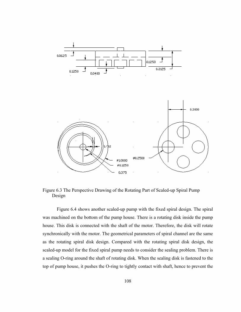
108

Figure 6.3 The Perspective Drawing of the Rotating Part of Scaled-up Spiral Pump Design

Figure 6.4 shows another scaled-up pump with the fixed spiral design. The spiral

was machined on the bottom of the pump house. There is a rotating disk inside the pump

house. This disk is connected with the shaft of the motor. Therefore, the disk will rotate

synchronically with the motor. The geometrical parameters of spiral channel are the same

as the rotating spiral disk design. Compared with the rotating spiral disk design, the

scaled-up model for the fixed spiral pump needs to consider the sealing problem. There is

a sealing O-ring around the shaft of rotating disk. When the sealing disk is fastened to the

top of pump house, it pushes the O-ring to tightly contact with shaft, hence to prevent the

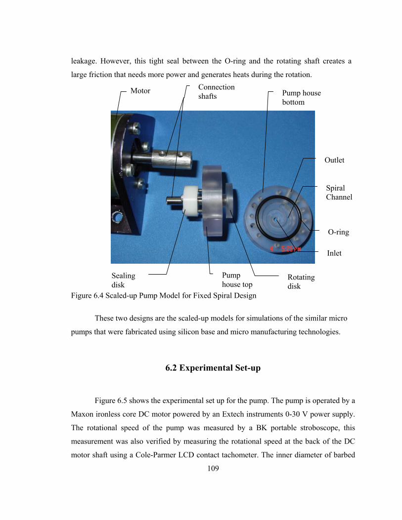
109

leakage. However, this tight seal between the O-ring and the rotating shaft creates a

large friction that needs more power and generates heats during the rotation.

Figure 6.4 Scaled-up Pump Model for Fixed Spiral Design

O-ring

Inlet

Spiral Channel

Outlet

Pump house bottom

Rotating disk

Pump house top

Sealing disk

Connection shafts

Motor

These two designs are the scaled-up models for simulations of the similar micro

pumps that were fabricated using silicon base and micro manufacturing technologies.

6.2 Experimental Set-up

Figure 6.5 shows the experimental set up for the pump. The pump is operated by a

Maxon ironless core DC motor powered by an Extech instruments 0-30 V power supply.

The rotational speed of the pump was measured by a BK portable stroboscope, this

measurement was also verified by measuring the rotational speed at the back of the DC

motor shaft using a Cole-Parmer LCD contact tachometer. The inner diameter of barbed

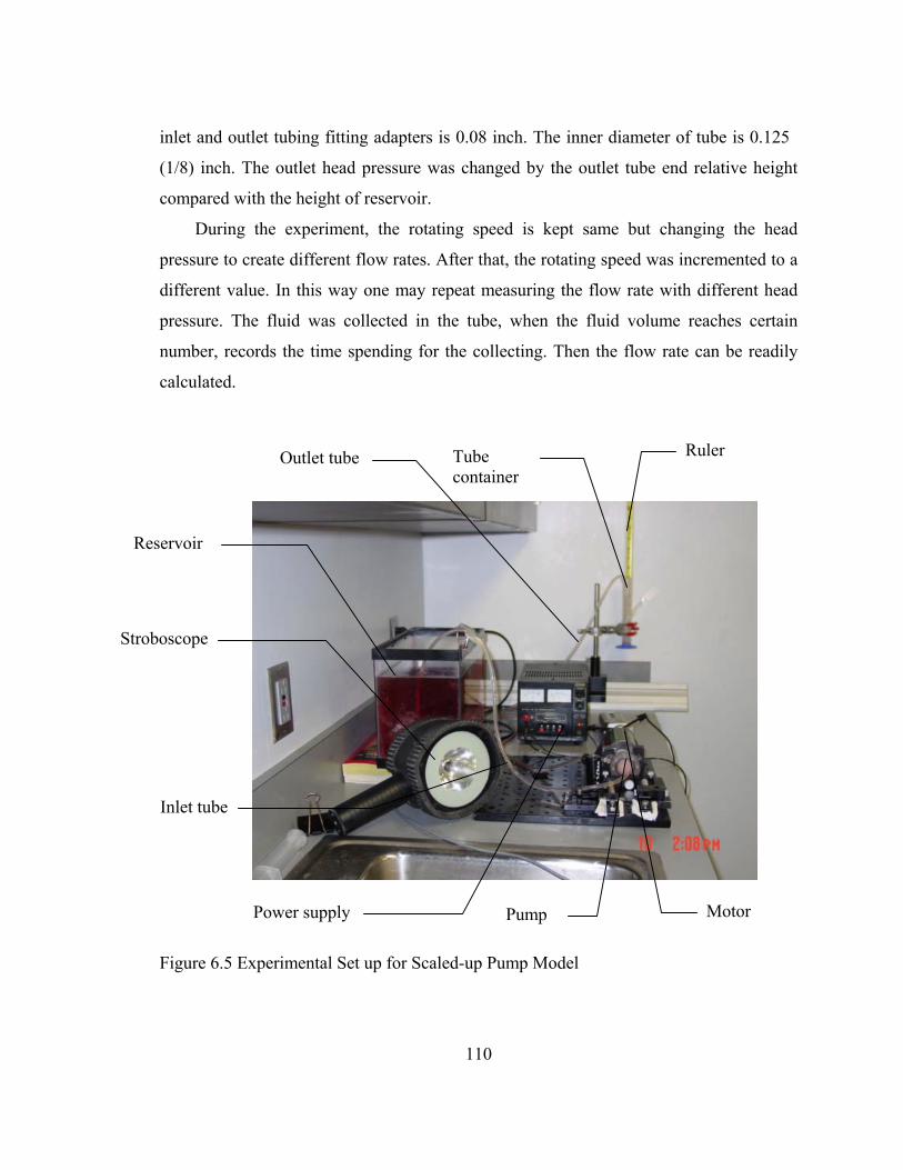
110

inlet and outlet tubing fitting adapters is 0.08 inch. The inner diameter of tube is 0.125

(1/8) inch. The outlet head pressure was changed by the outlet tube end relative height

compared with the height of reservoir.

During the experiment, the rotating speed is kept same but changing the head

pressure to create different flow rates. After that, the rotating speed was incremented to a

different value. In this way one may repeat measuring the flow rate with different head

pressure. The fluid was collected in the tube, when the fluid volume reaches certain

number, records the time spending for the collecting. Then the flow rate can be readily

calculated.

MotorPump Power supply

Inlet tube

Stroboscope

Reservoir

Outlet tube Tube container

Ruler

Figure 6.5 Experimental Set up for Scaled-up Pump Model

111

6.3 Experimental Results and Discussion

For the experiments of rotating spiral disk from the fist design, the gap distance h′

between the stationary disk (pump house top) and the top of wall of spiral protrusion is

0.1 mm. During the experiments, the spiral channel rotates clockwise as shown in figure

6.6. The stationary top cap is fastened to the pump house. The top cap presses the O-ring

so that the pump is sealed.

Figure 6.6 Rotation Direction of the Spiral Channel

When the spiral channel disk rotates clockwise, the fluid close to the top of the channel

sticks with the stationary top disk due to no slip boundary condition. The rest of fluid that

contacts with the other three sides of the channel was dragged forward in the direction of

the disk rotation. From the kinematics view, or from the viewpoint inside the channel,

the fluid in the top of the channel was dragged by the top disk to the outlet.

Figure 6.7 shows the relation of flow rate and pressure at different rotation

speeds. The adverse pressure is created by imposing a higher pressure at the outlet than

112

that at the inlet. Therefore, the result shows that the outlet the flow rate is almost linearly

decreasing function with the pressure head imposed. For example, the pump rotating at

at 3600 RPM under the adverse pressure of 6,000 pa with the set up shown in figure 6.7

will almost produce no net flow.

pressure vs flow rate

0

0.5

1

1.5

2

2.5

3

3.5

0 2000 4000 6000 8000 10000

pressure (pa)

flo

w r

ate

(m

l/s) 600 rpm

1200 rpm

1800 rpm

2400 rpm

3000 rpm

3600 rpm

4200 rpm

4500 rpm

Figure 6.7 Flow Rate versus Head Pressure of 2π Angular Span with the 0.1 mmGap

pressure vs flow rate

0

0.5

1

1.5

2

2.5

3

0 2000 4000 6000 8000

head pressure (Pa)

flo

w r

ate

(m

l/s)

600 rpm

1200 rpm

1800 rpm

2400 rpm

3000 rpm

3600 rpm

4200 rpm

4500 rpm

Figure 6.8 Flow Rate versus Head Pressure of 2π Angular Span with the 0.4 mmGap

When the distance h′ between the stationary disk (pump house top) and the top of

wall of spiral protrusion is increased from 0.1 mm to the 0.4 mm, the flow rate decreases

113

as shown in figure 6.8. This may be attributed to the cross flow in the gap between the

spiral and top cap. When this happens, the fluid in the top of the spiral channel does not

contact with the top stationary disk directly. The viscous force to drag the fluid along the

channel to the outlet is actually reduced. Hence, the viscous effect on the fluid in the

channel is diminished. The phenomenon is more pronounced when the gap distance

increases. The cross flow influence on the flow rate is exaggerated in higher pressures

from the comparison of figure 6.7 and figure 6.8.

When the total angular span of the centerline of spiral channel is close to 8π in the

same rotator with same channel depth and channel wall width, the flow rate versus the

pressure at different rotation speed are varied as figure 6.9 and figure 6.10 showed.

Head pressure vs flow rate

0

0.5

1

1.5

2

2.5

3

0 2000 4000 6000 8000 10000

Head pressure (Pa)

Flo

w r

ate

(m

l/s

) 600 rpm

1200 rpm

1800 rpm

2400 rpm

3000 rpm

3600 rpm

4200 rpm

4500 rpm

Figure 6.9 Flow Rate versus Head Pressure of 8π Angular Span with the 0.1 mmGap

114

Head pressure vs flow rate

0

0.5

1

1.5

2

2.5

0 2000 4000 6000 8000

head pressure (Pa)

flo

w r

ate

(m

l/s)

600 rpm

1200 rpm

1800 rpm

2400 rpm

3000 rpm

3600 rpm

4200 rpm

4500 rpm

Figure 6.10 Flow Rate versus Head Pressure of 8π Angular with the 0.4 mm Gap

The flow rate decreases for the setup with 8π angular span spiral channel when

compared with that of the 2π angular span spiral channel with the same head pressure and

same rotation speed. The reason is that the total fluid contained the channel decreases due

to the spiral channel wall occupying more volume of the pump house than that of the 2π

angular span spiral channel rotator. Less fluid is dragged in the 8π angular span spiral

channel per turn.

It is also interesting to investigate the influence of rotation direction on the spiral

pump flow rate. Experiments have been done when the spiral disk rotated with

counterclockwise direction instead of clockwise direction. The results are shown in figure

6.11. The pump used in the experiment has the 2π angular span spiral channel and the

gap distance h′ of 0.1 mm. The viscous drag from the stationary top disk to the fluid in

the spiral channel should have the negative effects to the flow rate. However, the

centrifugal force and the pump shape itself acting as the propeller dominates and the fluid

comes out of the outlet even with a relatively high head pressure.

115

Anti-RPM vs Highest head pressure

0

1000

2000

3000

4000

5000

6000

7000

8000

0 1000 2000 3000 4000 5000

Anti-RPM

Hig

he

st

he

ad

pre

ss

ure

Figure 6.11 The Highest Head Pressure the Pump Can Overcome (flow rate is 0 at this point) with Counterclockwise Rotation Direction

For the second spiral pump design, whose spiral channel was groove in the pump

house bottom as shown in figure 6.4, the testing results were quite different from the

rotating spiral channel design. The top disk rotates when the spiral channel keeps

stationary with the bottom. During the experiments, there is leakage problem through the

connecting shaft. Although there is O-ring with sealing disk to reduce the leakage, it is

difficult to provide the enough torque to the rotating disk when the O-ring was pressed

tight to the shaft. The flow rate is much lower than the rotating spiral channel disk design.

It also can barely overcome a very low head pressure.

6.4 Summary

This chapter discussed the performance of two fabricated scaled up pump

prototypes as simulations of micro spiral pumps’ performance. Through the comparison

of two designs, it is obvious that rotating spiral channel disk design have more

advantages. The different experiments showed that the spiral wall when rotated can help

116

to pump the fluid during pumping. The pump performance also depends on the

curvature ratio of the spiral, which will discuss in more detail in the next chapter.

Through the scaled up model experiments, the rotating spiral channel is recommended for

the fabrication in micro scale to the Sandia National Laboratories.

117

CHAPTER 7

NUMERICAL SIMULATION OF SCALED UP MODELS OF

MICROPUMP

7.1 Introduction

After the scaled up experiments for the micropumps, the numerical simulations for

the scaled-up and real micro models is performed in this chapter to improve and refine

the micropump designs and possibly to shorten the time required from the design to

fabrication of workable and marketable microdevices. The factors such as spiral

curvature ratio, pressure, fluid viscosity, tube geometry and package errors are studied

and discussed in the chapter based on the theoretical modeling and numerical simulation

results.

Before the numerical simulation of flow of the pump and the comparison with the

experimental results, it should be remarked fluid flow features in micro device may not

be the same as that in macro scale device. One may still predict the general fluid flow

from numerical simulations based on Navier-Stokes equations with non-slip-boundary

conditions at the wall provided that certain conditions are satisfied [3,97]. In this chapter,

the validity of the non-slip boundary conditions from microfluid flow simulation is

adopted and verified.

118

7.2 Characteristics of Fluid Flow in Micro-scale Device

One of important effect displacement by the fluid flow in the microdevice is

molecular effect that could induce slip flow at the wall. The traditional non-slip boundary

condition used in the continuum model may fail to provide accurate predictions for the

flow in the microdevices. If the traditional continuum model fails to regulate the liquid

fluid, then the more complicated molecular dynamic simulation seems to be the other

approach available to rationally characterize flow in microdevices. Such numerical

simulations are not yet well developed for realistic micro-scale flow. The microfluid

mechanics of liquids is much less developed than gases [97]. The molecular-based

models for gases were well developed. Liquid flow in micro device will be introduced

followed by introduction of some important concepts of the flow model for gases.

The continuum model is valid when mean free path λ in gas is much

smaller than a characteristic flow dimension L. The mean free path λ in a gas is the

average distance that molecules travel between the collisions with other molecules in the

gas. As a general guideline, macroscopic or continuum analysis cannot be applied to

situations that the characteristic length of the flow is of the same order as or lower than

the mean free path λ. λ is related to temperature T and pressure P as [3]:

(7.1)

where P is pressure, d is the molecular diameter and k is the Boltzmann constant

(1.38×10-23 J/K•molecule).

The ratio between the mean free and the characteristic length is known as

Knudsen number:

LKn

λ= (7.2)

119

If the Knudsen number is less than 10-3, Navier-Stokes equations with

non-slip boundary conditions are still valid for micro flow analysis. Table 7.1

summarizes the different Knudsen number regimes [3, 97].

Table 7.1 Knudson Number Regimes

Kn ~ 0 Kn < 10-3 10-3<Kn<10-1 10-1 <Kn<10 Kn ≥10

No molecular

diffusion;

Euler equations

Continuum

flow;

Navier-Stokes

equations with

non-slip

boundary

conditions

Slip-flow

regime;

Navier-Stokes

equations with

slip boundary

conditions

Transition

regime;

Moderately

rarefied

Free-molecule

flow;

Highly rarefied

The effects of molecular structure are quite different in gases and liquids. The

density of liquids is about 1000 times as the density of the gases; the spacing between

molecules in liquids is approximately ten times less than the spacing in gases. Liquid

molecules do not have a mean free path, but the lattice spacing, δ, may be used as a

similar measure. The lattice spacing δ is defined as [3]:

3/1

1~

AN

Vδ (7.3)

where 1V is the molar volume and N is Avogadro’s number. For water, this

spacing δ is 0.3 nm. For micro-spiral channel, the characteristic length L is the depth of

the channel. L is 5.8 µm that was designed in this study. The equivalent Knudsen number

is 5.17×10

A

-5. This number is well below 10-3. In this case, it is safe to assign the non-slip

boundary conditions for numerical simulation of the flow. Also, the scaled-up pump

model definitely has the macro-flow features including of the non-slip boundary

conditions.

120

Through the discussion of the boundary conditions situations in the micro

scale, it is clear that the liquid flow in micropump could be described adequately by

conventional continuum model from Navier-Stokes equations.

7.3 Formulation of Problems

7.3.1 Governing Equations

The numerical model may provide meaningful data for the performance of the

micropump which is difficult to quantitatively test in experiment. The data from scaled

up model experiment will be compared and verified with numerical simulation. The

numerical simulation after validated may provide the characteristic performance in the

same scale size of the micropump.

For the continuum model with constant viscosity, conventional Navier-Stoke

equations for incompressible flow in rectangular coordinates may be written as [98]:

∂∂

+∂∂

+∂∂

+∂∂

−=

∂∂

+∂∂

+∂∂

+∂∂

2

2

2

2

2

2

z

u

y

u

x

u

x

pg

z

uw

y

u

x

uu

t

ux µρυρ (7.4)

∂∂

+∂∂

+∂∂

+∂∂

−=

∂∂

+∂∂

+∂∂

+∂∂

2

2

2

2

2

2

z

v

y

v

x

v

y

pg

z

vw

y

v

x

vu

t

vy µρυρ (7.5)

∂∂

+∂∂

+∂∂

+∂∂

−=

∂∂

+∂∂

+∂∂

+∂∂

2

2

2

2

2

2

z

w

y

w

x

w

z

pg

z

ww

y

w

x

wu

t

wz µρυρ (7.6)

The continuum equation for incompressible fluid is written as:

0=∂∂

+∂∂

+∂∂

z

w

y

v

x

u (7.7)

121

There are four unknowns (p, u, v, w) in four equations. The velocity u, v and w

have second order differentiation with respect to x, y, z dimensions, and the pressure, p,

has a first order differentiation with respect to space. In each Navier-Stoke equation, the

velocity component has one order of differentiation with respect to time t. To solve these

equations for a unique solution, it is necessary to know seven boundary conditions and

one initial condition for each equations of (7.4)-(7.6).

7.3.2 Boundary Conditions for Governing Equations

Figure 7.1 shows the spiral pump control volume. To simpify the present

problem, the x-axis is assigned as the direction of channel width, the y-axis is assigned as

the direction of channel height, and the z-axis along the centerline the spiral channel. This

assumption of numerical simulation with Cartesian coordinates for Navier-Stokes

equtions is approximately valid if the channel width is small compared with the radius of

the channel curvature which is the case for the present study.

Figure 7.1 Outline of the Spiral Channel

122

The boundary conditions of the channel are listed as table 7.2 and table 7.3. As

the tables shown, there are totally 7 boundary conditions given in each equations.

Table 7.2 Boundary Conditions of Fixed-spiral Channel

X-Inner X-Outer Y-Bottom Y-Top Z-Inlet Z-Outlet

Non-slip

wall (u, v, w

=0)

Non-slip

wall (u, v,

w=0)

Non-slip

wall (u, v,

w=0)

Moving

wall(ω rad/s)

(u, w known,

v=0)

Total

pressure p1

Fixed

Pressure p2

Table 7.3 Boundary Conditions of Rotating Spiral Channel

X-Inner X-Outer Y-Bottom Y-Top Z-Inlet Z-Outlet

Moving

wall(ω rad/s)

Moving

wall(ω rad/s)

Moving

wall(ω rad/s)

Non-slip

wall

Total

pressure p1

Fixed

Pressure p2

we note that the velocity w, which is normal velocity to the channel cross section,

contribute to the net mass flow rate of the pump. Specify equation 7.6

∂∂

+∂∂

+∂∂

+∂∂

−=

∂∂

+∂∂

+∂∂

+∂∂

2

2

2

2

2

2

z

w

y

w

x

w

z

pg

z

ww

y

w

x

wu

t

wz µρυρ (7.6)

t

w

∂∂

may be neglected when it is steady. The boundary conditions for the fixed spiral

channel case are:

X at the spiral channel inner wall: w=0;

X at the spiral channel outer wall: w=0;

Y at the spiral channel bottom wall: w=0;

Y at the spiral channel top wall: w can be calculated from rotation speed ω, where ω is

the top disk rotation speed around the pump center axis;

Z at spiral channel inlet: either pressure P1, or inlet velocity w (z=0) is specified;

123

Z at spiral channel outlet: fixed pressure P2, or conservation of mass flow, or flow is

fully developed;

The boundary conditions for the rotating spiral channel case:

X at the spiral channel inner wall: w can be calculated from rotation ω;

X at the spiral channel outer wall: w can be calculated from rotation ω;

Y at the spiral channel bottom wall: w can be calculated from rotation ω;

Y at the spiral channel top wall: w =0;

Z at the spiral channel inlet: pressure P1, or inlet velocity;

Z at the spiral channel outlet: fixed pressure P2, or conservation of mass flow, or flow is

fully developed.

From figure 6.6, we notice that the surface area of the reservoir is much larger

than the cross area of the inlet tubing. Figure 7.2 gives the illustration of this situation,

where the inlet pressure P1is below the water surface level at P0.

Figure 7.2 Illustration of the Inlet Situation of Experiment

Considering the Bernoulli equation

1

2

110

2

00

22gz

WPgz

WP++=++

ρρ (7.8)

where W is approximately zero due to the relative large area of the reservoir compared

with that of inlet tube, the above equation could be rewritten as

0

124

)(2

100

2

11 zzgP

WP −+=+ ρ

ρ (7.9)

The left side of the equation (7.9) is defined as total pressure, which can be

calculated from the right side of the equation.

From this relation, we can rewrite equation (7.6) as

∂∂

+∂∂

+∂∂

+∂

+∂−=

∂∂

+∂∂

+∂∂

2

2

2

2

2

2

2

)2

(

z

w

y

w

x

w

z

wp

gy

w

x

wu

t

wz µ

ρ

ρυρ (7.10)

So, the total pressure may be considered as a specified known condition for

solving the equation (7.10). Now it is required to have 6 boundary conditions for each

unknown velocities to solve the governing equations (7.4-7.7). For specifying the

velocity w, the fixed pressure at the outlet is an equivalent boundary condition for the

velocity w in the z direction. There are four other boundary conditions for the velocity at

the x and y directions. The last boundary condition may be deduced from the continuity

equation: 0=∂∂

z

w.

The numerical simulation for the geometry shown in figure 7.3 is more

complicated than figure 7.1. However, both cases have similar boundary conditions.

Referring to figure 6.2 which shows the experiment model, the diameter of inlet and

outlet barbed tubing fitting adapters is 0.08 inch, the inner diameter of plastic tubes is

0.125 (1/8) inch. The tube connected to the inlet extends 20 inches long and the tube

connected to the outlet extends 40 inches long. Figure 7.3 shows the approximated

numerical simulation model invoking a hydraulic equivalent rectangular channel as its

outlet. The reason for this shape substitution of the outlet is only for the simplicity of the

grid generation in the numerical simulation. The flow media is water with density ρ of

997 kg/m3 and kinematic viscosity ν of 1.0× 10-6m2/s.

125

Figure 7.3 3-D View of the Numerical Simulation Model

7.4 Numerical Simulation

7.4.1 Numerical Simulation of rotating spiral model

As mentioned in the chapter 6, there are two different designs of micro spiral

pumps. In the first design, the spiral channel rotates, in another design, the top disk

rotates and the spiral channel with the substrate (the pump housing bottom for the scaled-

up model) is immobilized. In the first design, the fluid in the spiral channel moves with

when the pump runs. The upper side of the spiral channel is the stationary disk. The

viscous force between the static disk and fluid in channel drives the fluid to the outlet. At

the same time, the centrifugal force due to the rotating channel also contributes to push

the fluid to the outlet. In the second design, where the spiral channel is stationary, the

disk on the top of the spiral channel rotates. Hence, the viscous force between the disk

and fluid drags the fluid to the outlet. The centrifugal in this case will be small since the

spiral channel is stationary.

126

Spiral channel

Inlet

Outlet

Figure 7.4 Flow Grids of the Simulation Model

Figure 7.4 shows the grids for numerical calculation generated by CFDRC [100].

There are two group 3D grid data listed for verification purpose:

=====================================

Group 1: Summary of 3D Grid Data

=====================================

Total No. of nodes : 10280

No. of quad faces : 25330

Total No. of faces : 25330

No. of hexagon cells : 7629

Total No. of cells : 7629

=====================================

Group 2: Summary of 3D Grid Data

=====================================

Total No. of nodes : 27240

No. of quad faces : 73299

127

Total No. of faces : 73299

No. of hexagon cells : 23112

Total No. of cells : 23112

=====================================

Group 3: Summary of 3D Grid Data

=====================================

Total No. of nodes : 113502

No. of quad faces : 300868

Total No. of faces : 300868

No. of hexagon cells : 93985

Total No. of cells : 93985

The difference of flow rate results from group 1 and group 2 is less than 5%. The

difference of flow rate results from group 2 and group 3 is less than 3%. The third group

grid number is large enough to achieve the numerical results independent of grids. The

numerical simulation results (mass flow rate, gram/second) are shown as figure 7.5.

0

0.2

0.4

0.6

0.8

1

1.2

1.4

1.6

0 1000 2000 3000 4000 5000

rpm

g/s

Figure 7.5 Numerical Simulated Mass Flow Rates versus Different Spiral Rotation Speed

128

From the mass flow rate, average flow velocity in the channel could be

calculated:

V =(mass flow rate)/(channel cross area).

When pump rotates at 1800 rpm without head pressure, which means the outlet

pressure and inlet total pressure are the same. The average Reynolds number in

simulation is:

νLV

=eR =(9.31×10-4 kg/s / (997 kg/ m3×11.7 mm2) × 3.175 mm)/1.0× 10-6m2/s=253

The depth of the spiral channel (groove) is 0.125 inch, the width of the channel is

0.145 inch, the cross area is 11.7 mm2, the density of water is 997 kg/ m3, the feature

length is the channel depth which is 3.175mm. The maximum velocity Vmax of the fluid

in the channel is at the boundary with the outset spiral wall with rotates with the spiral:

Vmax =ω×r=188.4 rad/s × 10.5 mm =1.978 m/s

If we use this velocity to estimate the maximum Reynolds number of the channel, it

is:

Re=1.978 m/s × 3.175 mm/1.0× 10-6m2/s =6280.

Figure 7.6, 7.7 and 7.8 present the velocity distribution at different position in the

channel when the spiral channel rotates at 1800 rpm clockwise.

129

Figure 7.6 Velocity Contour on the Top of the Rotating Spiral Channel @1800 rpm

Figure 7.7 Velocity Contour on the Bottom of the Rotating Spiral @1800 rpm

Figure 7.8 Velocity Contour in Rotating Spiral Channel Cross Section @1800 rpm

130

Figure 7.9 Pressure Distributions on the Middle of the Rotating Channel @1800 rpm

Fluids near the top of channel contacts with a static top disk while the other three

sides of the fluid are adjacent to the rotating wall of the spiral. Due to the no-slip

boundary conditions, the fluid adjacent to the top disk keeps static when the thin layer of

fluid adjacent to the other sides rotates with walls of the channel. In the figure 7.8, the left

side is the outside of the channel, so the fluid flow over there is larger than the flow close

to the inner side of the channel when the channel is rotating. Figure 7.9 gives the pressure

distribution in the channel. From the figure, the pressure decreases from the inlet along

the spiral to the end of the spiral.

7.4.2 Numerical Simulation of fixed spiral model

In the fixed spiral channel design, the spiral channel keeps stationary and the top

disk rotates. Hence, the viscous force between them could make the flow to outlet. Figure

6.5 shows the scaled-up model of fixed spiral for experiment. In the experiment, this

131

fixed spiral model pump barely works when the total pressure of inlet and fixed pressure

of outlet are the same. The pump can only hold about 2-3 inches water height higher than

reservoir water level. However, the numerical simulation still gives a result that is close

to the simulation result of the rotating spiral channel. Figure 7.10 plots the mass flow rate

versus different rotating speed of the top disk. The total pressure of inlet keeps the same

as the fixed pressure of the outlet.

0

0.2

0.4

0.6

0.8

1

1.2

1.4

1.6

1.8

0 1000 2000 3000 4000 5000

Rotating speed (rpm)

Mass f

low

rate

(g

/s)

Figure 7.10 Numerical Simulated Mass Flow Rates versus Different Top Disk Rotation Speed

Figure 7.11, 7.12 and 7.13 present the velocity distribution in the channel when

the top disk rotates at 1800 rpm in the counterclockwise direction. Compared with figure

7.11 and figure 7.12, we notice that the viscous effect due to top rotating disk to the fluid

in the channel decays very fast.

132

Figure 7.11 Velocity Contour on the Top of the Spiral Channel @1800 rpm

Figure 7.12 Velocity Contour on the Plane 5% Below the Top Disk @1800 rpm

Figure 7.13 Velocity Contour in Fixed Spiral Channel Cross Section @1800 rpm

133

Figure 7.14 Pressure Distribution Below the Top Disk @1800 rpm

Comparison of pressure distribution in figure 7.14 with that in figure 7.9, which

giving the pressure distribution of the rotating spiral shows that the scale of pressure in

the fixed spiral is less than the pressure in the rotating spiral pump. The reason is that the

rotating channel could create centrifugal force to press the fluid while the centrifugal

force in the fixed spiral channel design is negligible.

7.5 Discussion of Numerical Simulation Results

Though the moving parts are different in two designs, the mass flow rates

predicted from numerical simulation are close as figure 7.5 and figure 7.10 shown. As

mentioned before, the scaled up model experiment of fixed spiral channel pump do not

work well, while another design with rotating spiral channel can pump fluid much better

than the fixed spiral scaled up design, as shown in figure 7.15.

The fluid flow analytical simulations where the spiral channel does not rotate and

the top disk rotates, is given conditionally in kilani’s paper [100]. The numerical

simulation of mass flow rate by CFDRC matches well with his theoretical flow rate by

solving the Navier-Stoke equations under unfolding approximation in a straight-channel

model for the flow field in the spiral channel. As far as the rotating spiral channel

134

situation is concerned, the problem is more complicated than that of the stationary spiral

channel.

0

0.5

1

1.5

2

2.5

3

3.5

0 1000 2000 3000 4000 5000

rpm

g/s

Figure 7.15 Experimental Mass Flow Rates at Different Rotation Speed without Head Pressure

Figure 7.16 Outlet Position 1 of Rotating Spiral

Figure 7.17 Outlet Position 2 of Rotating Spiral

When the spiral channel is rotating, the stationary outlet position will appear to

changing from the rotating spiral viewpoint. Figure 7.16 shows outlet position at one time

and figure 7.17 shows outlet positions relative to the spiral when the spiral channel

135

rotation of 90 degree. The numerical simulation results give 25% difference of the mass

flow rates in two cases when the rotation is at 1800 rpm. This fact tells us that the

CFDRC numerical simulation could not predict effectively to the simulation due to the

moving outlet position, especially for the asymmetric geometry such as our spiral

channel. The numerical simulation results in figure 7.16 and figure 7.17 are achieved

without considering the actually outlet connected tubing length which is around 45

inches. If this factor is considered, the mass flow rate should decrease. For example, the

mass flow decreases from 0.93 g/s to 0.41 g/s when the rotating speed is 1800 rpm. The

actually mass flow rate in this situation measured in experiment is 1.04 g/s. This may be

attributed to the wall of the spiral channel acting as a propeller when it rotates and the

effect of centrifugal force.

It is valuable to set-up an analytic mathematical model for the flow in the channel to

study different effects. As the flow enters a curvature site such as spiral channel, the fluid

is being forced to change direction to follow the curve and hence a radial pressure

gradient develops between the outer and inner wall of curvature. The fluid is also

subjected to centrifugal force that is proportional to the square of the axial velocity. In the

case of inviscid flow, these two forces balance each other and hence the axial velocity

profile is skewed towards the inner wall of curvature and almost no secondary flow

develops. With viscous fluid, the two opposing forces do not balance each other because

the fluid near the flow axis which have a higher velocity due to a larger centrifugal force

than the slower particles near the walls. Hence a secondary flow develops. Dean number

determines the influence of curvature in the laminar case [98]:

r

RRV

r

RRD e υ

==2

1 (7.11)

Where R is the radius of the cross-section and r is the radius of curvature.

The resistance λ to flow caused by the curvature pipe compared with the

resistance λ0 in a straight pipe given by L.Prandtl [98]:

136

36.0

0

37.0 D=λλ

(7.12)

This equation gives good agreement with experimental results in the range:

0.36.1 10Re10 <<r

R (7.13)

For the scaled up model, the Re is 253, hence the Dean number is

r

RRV

r

RRD e υ

==2

1=0.5×253×(1.7 /10.5 )0.5=51

R is hydraulic diameter given by

PerimeterWetted

AreaSectionCrossR

_

__2×= =2×(0.125×0.145)/(2×(0.125+0.145))=0.134″ =1.7 mm

The sizes of 0.125″ and 0.145″ in the above formula are the depth and width of the

scalped-up rectangular spiral channel respectively.

The resistance λ to flow caused by this scaled-up model in the above case, which

Re is in the limit (equation 7.13) of application of equation 7.12, is compared with the

resistance λ0 in a unfolding straight channel:

36.0

0

37.0 D=λλ

=1.52

This analysis is very approximate and it is only to help to explain that the

unfolding straight channel is not approximate for the scaled-up model in the experiment

besides the large Reynolds number itself make a large leading-order error in the axial

137

velocity due to the unfolding approximation is proportional to the square of Reynolds

number [101]. The analytic solution for this case is difficult to achieve due to its

geometry. The numerical simulation based on finite element method may be suitable for

solving the problem.

The micro spiral pump geometry is listed in table 7.4. The centerline curve of the

spiral channel is designed in polar coordinates by:

θθθ ∆≤≤+= 0,0rkr (7.14)

Table 7.4 Spiral Geometry Parameters in Micro Pump Design

Parameter Value

Polar slope k 12 um

Starting radius r0 146 um

Angular span ∆θ 8π

Channel Height h 5.8 um

Channel width w 54 um

According equation 7.14, the maximum radius of the micro spiral pump is 287

um.

Re=Vh/ν=ωrh/ν=ω( 0rk +θ )/ν

ν is fluid (water) kinematic viscosity which is 1.0× 10-6m2/s here. ω is the top disk

rotation speed. r is the radius of spiral at certain angular span θ. For instance, when ω is

1800 rpm, Re number at spiral channel maximum radius is 0.5. This low Re number

indicates the viscous effects is dominated in the flow. As the rotation speed increases,

inertial effects increases to be comparable to the viscous effect in the micro channel. This

low Reynolds number is out of the limit of range which can use Prandtl model (equation

7.12) to predict the relative resistance to the flow compared with one in unfolding straight

138

channel case. In this micro spiral pump, the curvature ratio rw /=ε (w is the width of

channel and r is radius of curvature channel) and Re are very small. So the unfolding

approximation is valid, part of total flow rate due to viscous drag by the stationary

boundaries could be given by [100]:

pr

whwhrQ

a

a ∆∆

−=θµ

ω122

3

(7.15)

where 02

rkra +∆

=θ

, is pressure difference between the outlet and inlet of the spiral

channel.

p∆

The numerical simulation results of micro spiral channel pump meet the

theoretical expectation by equation (7.15) in the above conditions [106]. When the spiral

channel curvature changes, for example, the curvature ratio 0/ rw=ε increases to 0.56 as

the scaled up model, the unfolding assumption is not satisfied due to the large curvature

ratio. We still use CFD software package to simulate in this situation.

This section explains the difference between experimental and numerical

simulation results for the scaled up model. The comparison between scaled-up model

experiment results and numerical simulation results indicates that one could not only

focus on the flow in the pump channel. It also requires considering the effect of pump

rotational wall in the final flow rate out the outlet in the real working situation. In this

section, some useful analysis equations for analyzing the flow in the channel are also

given and discussed with the pump characteristics.

7.6 Summary

In this chapter, the continuity problem of the micro-scale channel is discussed.

The governing equation for the flow in the channel and relative boundary conditions are

given which help to set up the numerical simulation for the spiral pump. The numerical

simulations of two different scaled-up models for micro spiral pumps are given in the

139

chapter. Through the comparison and discussion between the experimental results and

numerical simulation results, we found that the effect of rotating asymmetric spiral wall

geometry may be an important factor to effect the final flow rate of in situ pumping

condition which we did not considered before the scaled-up experiment. The analytical

model for spiral pump based on unfold channel approximation is also discussed, the

analytical solution of micro spiral pump is verified by the numerical simulations.

140

CHAPTER 8

CONCLUSIONS AND RECOMMENDATIONS

8.1 Summary of Magnetic-MEMS Research

The present study investigates magnetic coupling in the MEMS and its

application in micropumps. Magnetic material deposition techniques and material

properties on micro devices were first studied. Then magnetic driven mini screw pumps

and magnetic driven gear systems were designed and discussed. The magnetic driven

gear system may be used to actuate the micro pump. The performance characteristics of

the microfluidics and micro spiral pump are investigated and evaluated by the scaled-up

experimental and numerical simulation methods.

8.1.1 Magnetic Material Deposition and Magnetic Coupling

The pulsed laser deposition (PLD) method was used in growing magnetic film on

silicon substrate. The study focused on achieving high magnetic susceptibility properties

for the magnetic film. Effects of (1) substrate temperature and (2) external magnetic field

on the magnetic material growing were considered in the depositing process. The

experiment showed that when the film was deposited on the substrate at the room

temperature or 250°C, the applied external perpendicular magnetic field could improve

the amorphous film magnetization remanence at the same direction. As temperature

increases to 500°C, some minor Nd2Fe14B crystalline phases showed in the X-ray

Diffraction patterns and the external magnetic field has negligible effect in the film

formation. When substrate temperature increases to 650oC, no major Nd2Fe14B crystalline

141

phase was formed. The low intensity peaks of Nd2Fe14B crystalline phase indicate the

film magnetic properties are soft. No obvious magnetic crystalline anisotropy showed

after the correction of shape (geometry) anisotropy. Along the external magnetic field, a

higher remanence film may be achieved comparing with the film deposited without

external field. However, This phenomenon will be weakened with the temperature

raising. PLD is a convenient lab method to implement as the addition step for magnetic

material deposition to the micro device surface. In the present study, the magnetic

material deposition is a post-microfabricature processing after the micro devices are

fabricated from Sandia National Laboratories standard micro fabrication procedures

(SUMMiT) which could not integrate with the magnetic material deposition process. This

two-step fabrication process also creates many challenges to make the magnetic micro

devices a popular MEMS applications.

There are certain advantages of the magnetic driven systems. For example, A

magnetically driven mini screw pump that was designed and fabricated for pumping

biological fluids such as blood. The magnetically driven pumps offer (1) remote coupling

of driving torque, (2) complete sealing of the pump housing except the inlet and outlet, (3)

contamination free pumping and (4) insulation of heat conduction from the pump shaft.

The performance characteristics of the magnetically driven pump were obtained

experimentally. The experiment demonstrates that mini-screw pump with a detached

magnetic driven system is able to pump the fluid with a rotating screw enclosed in

cylindrical in a cylindrical case. Two poles magnets couplings were used to transfer the

torque from outside motor to inside screw core remotely. This seal-less and self-

contained magnetic driven mini screw pump operates smoothly without a shaft crossing

its housing during the experiment. In blood flow applications, this design was shown to

eliminate the possibility of blood leakage through the seals. Another advantage of this

design is that it allows the pump to be designed as a disposable device eliminating the

possibility of bio-contamination from the more expensive driving system.

Magnetic force and torque for the magnetic driving mechanism are important

factors to judge whether the design of magnetically driven micro devices such as

microgear system or micropump satisfies the expectation. The magnetic coupling force

142

and torque between the driving part and driven part depend on several factors such as

the number of the interacting poles, the separation distance, the strength of the magnets or

the magnetic properties of the film, and the angle offset between the magnetic coupling

setting. From both fundamental and applied viewpoints, theoretical computation study of

the force and torque of a magnetic coupling or magnetic particles is very useful for

prediction and comparison purposes with the experimental results. Mathematically

analytic formulas for magnetic coupling force and torque and governing equations with

their relative boundary and continuity conditions for finite element analysis of the

magnetic related parameter solutions were presented in the dissertation. Commercial

package AMPERES based on boundary element method was used for numerical

simulations for magnetic coupling. The magnetic force and torque simulation results

provide important references for the magnetic coupling design.

8.1.2 Magnetic MEMS and Micropumps

Magnetic MEMS present a new class of micro devices with great potential and

applications. Improving the conventional MEMS by incorporating magnetic materials as

the sensing or actuating element offers new capabilities and open new markets for the

information technology, automotive industry, biomedical devices, space and

instrumentation. Magnetic MEMS are based on electromagnetic or magnetic interactions

between magnetic materials and active electromagnetic coils or passive magnetic field

sources such as permanent magnets. Magnetic materials can be deposited on micro

device that can be remotely manipulated by magnetic driving components. At the

micrometer scale, magnetic MEMS offer distinct advantages as compared with

electrostatic and piezoelectric actuators in strength, polarity and distance of actuation.

The first application is to replace the current electrostatic actuator in some situations.

Detail design and fabrication procedures were described in the dissertation. Magnetically

driven micro gear was fabricated by growing a thin film of rare earth magnetic material

on a driving gear surface using pulse laser deposition. From magnetic coupling with

outside magnets, the magnetized micro gear may transfer the torque to the micro moving

parts such as micro pump by gear trains.

143

Experimental study shows that micropump is able to pump the fluid. Due to the

lack of microfabrication and testing facilities, it is difficult to test experimentally in the

micro scale to acquire quantitative pumping performance. Scaled-up models were built to

verify the micro spiral pump concept and investigate relative pumping characteristics.

Numerical simulation of the flow in the pumps was also presented in the dissertation.

Numerical simulations for two designs of the micro-scale pumps were made. The first

design has a rotating top disk with spiral channel. In the second design, the spiral is

stationary with the substrate while the top disk rotates alone. The rotating parts in both

designs are driven by microengine such as electrostatic actuators or magnetic coupling.

The continuity problem of the micro-scale channel was also discussed. Before the

numerical simulation it was investigated the flow in the small scale at the micrometers

since it may have molecular effects such as wall slip which may be more important than

before and traditional continuum model may fail to provide accurate predictions for the

flow. From the analysis, the Knudsen number is a key reference to define the boundary

conditions for different flow regimes. Navier-Stoke equations with no-slip boundary

conditions are still valid for simulations of the channel flow in the micro-spiral pump.

Details of boundary conditions were given which were acquired for the numerical

simulation. The scaled up models used in the experiment provided the data. Through the

comparison and discussion between the experimental results and numerical simulation,

the role of rotating asymmetric spiral wall geometry is investigated and it may be a factor

to effect the final flow rate of in situ pumping condition. The rotation spiral pump design

is more efficient to pump fluid than the fixed spiral pump design is. The efficiency

difference will decrease when the spiral curvature rw /=ε (w is the width of channel and

r is radius of curvature channel) reduces.

144

8.2 Future Prospects of the Relative Research

1. To develop micro electromagnetic motors, one may arrange coils around a high

susceptibility magnetic pillar to produce appropriate magnetic flux for coupling the

magnetic thin film which was deposited on the surface on the micro rotation devices such

as gear or disk. There are some literatures [29,81,102] reporting the design of magnetic

MEMS. Whether the electromagnetic field strength is able to drive micro-size and to

mini-size device is still under investigation. However, the fabrication convenience and

cost of micro electromagnetic motor are important factors to be considered in the future

magnetic MEMS design.

2. The effect of the spiral geometry on the mass flow rate needs further

investigation by experiment and simulation. From the experiment investigation and

numerical simulation by varying the spiral channel’s geometry, an appropriate geometry

parameters for the spiral pump may be found to pump more efficiently than current

design.

3. In the dissertation, the magnetic coupling is used as driving principle to design

the microactuator. It should be remarked that recently application of micro or nano

magnetic particles becomes increasingly popular in cell sorting and separation. The

general approach involves the use of paramagnetic particles coated with antibodies

against the target cell surface. Then an external magnet or other magnetic source is

imposed to achieving the sorting or separation. This immunomagnetic separation

technology has been applied to removal harmful cells from blood or to make

immunomagnetic assays for clinical diagnostics. Since magnetic field can be used to

capture the micro or nano size magnetic particles the present research in magnetic driven

mechanism may apply to develop inexpensive single cell manipulating array, The

investigation for the magnetic force and torque on a single magnetic particle were already

included in the dissertation. These efforts may be extended to the design of cell sorting

or cell array devices.

145

4. Magnetic thin film was grown in the research. It is noted that there are many

studies made in this area. However, the effects of the external field on the magnetic films

properties during the PLD deposition process still requires further investigation. The

micro fabrication techniques to make micro-magnets are very important. There is great

potential usage of micro-magnets to sensors, telecommunications and biomedical

applications.

The present work only presents the preliminary study on the Magnetic-MEMS

and Micro-fluidics. The research in these two areas grows rapidly because the

applications of the magnetic MEMS and microfluidics are developed in life science and

nano science as well as in the electrical industry.

146

REFERENCES

[1] R. P Feynman, (1961), “There’s Plenty of Room at the Bottom,” Journal of Microelectromechanical Systems, vol. 1, no.1, March 1992, pp. 60-66.

[2] R. P. Feynman, (1983), “Infinitesimal Machinery”, Journal of

Microelectromechanical Systems”, vol.2, no.1, March 1993, pp. 4-44. [3] Mohamed Gad-el-Hak, “The MEMS Handbook”, CRC Press, 2001. [4] K. H. –L. Chau, et al., “An Integrated Force-balanced Capacitive Accelerometer

For Low-G Applications”, Proc. 8th Int. Conf. on Solid State Sensors and Actuators, Stockholm, Sweden, June 1995, pp 593-596.

[5] L. J. Horbeck, T. R. Howell, R. L. Knipe and M. A Mignardi, “Digital Micromirror

Device – Commercialization of a Massively Parallel MEMS Technology”, MEMS Symposium, ASME IMECE, November 1997, pp. 3-8.

[6] J. Darabi, M. M. Ohadi, and D. DeVoe, “An Electrohydrodynamic Polarization

Micropump for Electronic Cooling”, Journal of Microelectromechanical Systems, vol.10, no.1, March 2001, pp. 98-106.

[7] Committee on Advanced Materials and Fabrication Methods for

Microelectromechanical Systems, “Microelectromechanical Systems-Advanced Materials and Fabrication Methods”, National Academy Press, Washington, D.C. 1997.

[8] T. R. Hsu, “MEMS & Microsystems Design and Manufuacuture”, McGraw-Hill 1st

ed. 2002. [9] Nadim Maluf, “An Introduction to Microelectromechanical Systems Engineering”,

Artech House, 2000. [10] C. J. Kim, A. P. Pisano, and R. S. Muller, “Overhung Electrostatic Microgripper”,

Technical Digest, IEEE International Conference on Solid-State Sensors and Actuators, San Francisco, 1991, pp.610-613.

147

[11] E. J. Garcia, and J. J. Sniegowski, “Surface Micromachined Microengine as the Driver for Micromechanical Gears”, in Digest Int. Conf. on Solid-State Sensors and Actuators, June, Stockholm, Sweden, 1995, pp. 365–368.

[12] W. S. Trimmer, K. J. Gabriel, “Design Considerations for a Pratical Electrostatic

Micro Motor”, Sensors & Actuators, vol. 11, 1987, pp. 189-206. [13] Sandia National Laboratories, “ MEMS Short Courses”, 2000. [14] R. Zengerle, M. Richter, and H. Sandmaier, “A Micro Membrane Pump with

Electrostatic Actuation”, Proceedings of IEEE Micro Elctro Mechanical systems workshop, Travemunde, Germany, February 1992, pp 19-24.

[15] http://www.ansys.com/ansys/mems/mems_applications/app_thermal_actuator.htm [16] A. K. Henning, J. Fitch, etc.,”A thermopneumatically Actuated Microvalve for

Liquid Expansion and Proportional Control”, Proceedings, transducers’97, IEEE Conference on Sensors and Actuators, June 1997, pp.825-828.

[17] A. K. Henning, “Micorfluidic MEMS”, IEEE Aerospace Conference, Snowmass,

Colorado, March 25, 1998. [18] Clements, Ken, U.S. Patent No. 6,588,208, "Wireless Technique for

Microactivation"

[19] K. J Gabriel, W. S Trimmer, and J. A Walker, “A Micro Rotary Actuator Using Ahape Memory Alloys”, Sensors and Actuators, vol.15, no.1, 1988, pp.95-102.

[20] P. Krulevitch, A. P. Lee, P. B. Ramsey, J. C. Trevino, J. Hamilton, and M. A.

Northrup, “Thin Film Shape Memory Alloy Microactuators”, Journal of Microeletromechanical Systems, vol.5, 1996, pp. 270-281.

[21] T. Higuchi, U. Yamagata, K. Furutani and K. Kudoh, “ Precise Positioning

Mechanism Utilizing Rapid Deformations of Piezoelectric Elements”, Proceedings of IEEE, Micro Electro Mechanical Systems, February 1990, pp. 222-226.

[22] J. W. Judy, D. L. Polla and W. P. Robbins, “Experiemental Model And IC-Process

Design of a Nanometer Linear Piezoelectric Stepper Motor”, MicroStructures, Sensors and Actuators, DSC-vol. 19, November 1990, pp. 11-17.

[23] G.-A. Racine et al, “Hybrid Ultrasonic Micromachined Motors”, MEMS 1993

Proceedings, pp. 128-132 [24] Seiko Instruments Inc. “Micro Piezoelectric Motor”.

148

[25] J. Y. Park and M. G. Allen, "Development of Magnetic Materials and Processing

Techniques Applicable to Integrated Micromagnetic Devices", Journal of Micromechanics and Microengineering, vol. 8, May 1998, pp. 307-316.

[26] D. J. Sadler, T. M. Liakopoulos, and C. H. Ahn, "A Universal Electromagnetic

Microactuator Using Magnetic Interconnection Concepts", Journal of Microlectromechanical Systems, vol. 9, no. 4, 2000, pp.460-468.

[27] E. T. Carlen and C. H. Mastrangelo, “Simple, High Actuation Power, Thermally

Acitivated Paraffin Microactuator”, Transuducers’99 conference, Sendai, Japan, June 1999.

[28] S. F. Bart, T. A. Lober, R. T. Howe, J. H. Lang and M. F. Schlecht, “Design

considerations for micromachined electric actuators”, Sensors and Actuators, vol.14, July 1988, pp.269--292.

[29] M. Barbic, Magnetic wires in MEMS and bio-medical applications, Journal of

Magnestism and Magnetic Material, vol. 249, 2002, pp. 357-367. [30] D. Niarchos, “Magnetic MEMS: Key Issues and Some Applications”, Sensors and

actuators, A. 106, 2003, 255-262. [31] P. Zheng, Y. Haik and C. J. Chen, “The Application Of Magnetic Coupling In

Micro Devices ”, ASME 2003, Washington DC, November 2003. [32] Y. Haik, M. Kilani and C. J. Chen, “Development of Magnetic MEMS”, 3rd

International Conference on the Scientific and Medical Applications of Magnetic Carriers, Rostock, Germany, May 1-6, 2000.

[33] V.M. Pai, “Experimental and Theoretical Study of Biomagnetic Fluid Dynamics”,

Ph.D. dissertation, department of M.E., Florida state university, summer, 1997. [34] Y. Haik, V. Pai and C. J. Chen, “Development of Magnetic Device for Cell

Separation”, Journal of Magnetism and Magnetic Materials, vol. 194, no. 1-3, April 1999, pp. 254-261.

[35] J. W. Judy, “Batch-fabricated Ferromagnetic Microactuators with Silicon Flexures”,

PhD dissertation, University of California, Berkeley, 1996 [36] J. W. Judy and R. S. Muller, “Magnetically Actuated, Addressable Microstructures”,

Journal of Microelectromechanical Systems, vol. 6, no. 3, 1997, pp. 249-56.

149

[37] Finn Jorgensen, “The Complete Handbook of Magnetic Recording”, 4th edition, McGraw-Hill 1995.

[38] T. Fukuda and W. Menz, “Micro Mechanical Systems: Principles and

Technology”, Elsevier Science 1998. [39] D. B. Chrisey and Graham K. Hubler, “Pulsed Laser Deposition of Thin Films”,

John Willy &Sons, Inc. 1994. [40] S. O. Kasap, “Principles of Electrical Engineering Magnetials and Devices”,

McGraw-Hill Higher Education, 2000. [41] M. Sagawa and S. Hirosawa, “Magnetic Hardening Mechanism in Sintering R-Fe-B

Permanent Magnets,” Journal of Materials Research, vol. 3, no. 1, 1988, pp. 45-54. [42] J. J. Croat, J. F. Herbst, R. W. Lee, and F. E. Pinkerton, “High-energy product Nd-

Fe-B permanent magnets”, Applied Physics Letters, vol. 44, no. 1, 1984, pp. 148-151.

[43] B. Wagner, M. Kreutzer and W. Benecke, “Permanent Magnet Micromotors on

Silicon Subtrate”, Journal of MEMS, vol.2, no.1, March 1993, pp. 23-29. [44] H. H. Yang etc., “Ferromagnetic Micromechanical Magnetometer”, Sensors and

Actuators, A 97-98, 2002, pp. 88-97. [45] T. S. Chin, “Permanent Magnet Films for Applications in Microelectromechanical

Systems”, Journal of Magnetism and Magnetic Materials, vol. 209, no. 1-3, February 2000, pp. 75-79.

[46] A. S. Kim and F. E. Camp, “High Performance of NdFeB”, Journal of Applied

Physics, vol. 79(8), 1996, pp. 5035-5039. [47] K. D. Aylesworth, Z. R. Zhao, D. J. Sellmyer and G. C. Hadjipanayis, “Magnetic

and Structural Properties of Nd2Fe14B Permanent-magnet Films and Multilayers with Fe and Ag”, Journal of Applied Physics, vol. 64(10), 1988, pp. 5742-5744.

[48] H. Jiang, J. Evans, J. J. O’Shea and J. Du, “Hard Magnetic Properties of Rapidly

Annealed NdFeB Thin Films on Nb and V Buffer Layers”, Journal of Magnetism and Magnetic Materials, vol. 224, 2001, pp. 233-240.

[49] S. Yamashita and J. Yamasaki, “Anisotropic Nd-Fe-B Thin-film Magnets for Miliz-

size Motor”, Journal of Applied Physics, vol. 70, no.10, 1991, pp. 6627-6629.

150

[50] C. J. Yang, S. W. Kim and J. S. Kang, “Magnetic Properties of NdFeB Thin Films Grown by a Pulsed Laser Deposition”, Journal of Magnetism and Magnetic Materials, vol. 188, 2001, pp. 100-108.

[51] C. J. Yang, E. B. Park, “ The Effect of Magnetic Field Treatment on the Enhanced

Exchange Coupling of a Nd2Fe14B/Fe3B Magnet”, Journal of Magnetism and Magnetic Materials, vol. 166, 1997, pp. 243-248.

[52] S. N. Piramanayagam, M. Mastsumoto and A. Morisako, “Thickness Dependence

of Magnetic Properties of NdFeB Thin Film with Perpendicular Magnetic Anisotropy”, Journal of Magnetism and Magnetic Materials, vol. 212, 2000, pp. L12-L16.

[53] J. Douglas Adam, Handbook of thin film devices (volume 4), Magnetic Thin Film

Devices, Academic Press 2000. [54] K. Chen, H. Hegde, S. U. Jen and F. J. Cadieu, “Different types of anisotropy in

amorphous SmCo films”, Journal of Applied Physics, vol.73, no.10, 1993, pp. 5923-5925.

[55] K. Chen, H. Hegde, and F. J. Cadieu, “Induced anisotropy in amorphous Sm-Co

sputtered films”, Applied Physics Letter, vol. 61 no.15, 1992, pp. 1861-1863. [56] G. Suran, K. Ounadjela and F. Machizaud, “Evidence for Structure-Related Induced

Anisotropy in Amorphous CoTi Soft Ferromagnetic Thin Films”, Physical Review Letters, vol. 57, no. 24, December 1986, pp. 3109-3112.

[57] P. Zheng, Y. Haik, M. Kilani and C.J. Chen, “ Froce and Torque Characteristics for

Magnetically Driven Blood Pump”, Journal of Magnetism and Magnetic Materials, vol. 241, 2002, pp. 292-302.

[58] F. T. Ulbay, “Fundamentals of Applied ElectroMagnetics”, Prentice Hall, 1996. [59] J. D. Jackson, “Classical Electrodynamics”, Second edition, John Wiley&

Sons.1975 [60] M. Zborowski, L. Sun, L.R. Moore, P. S. Williams and J. J. Chalmers, “Continuous

cell separation using novel magnetic quadrupole flow sorter” Journal of Magnetism and Magnetic Materials, vol. 194, 1999, pp. 224-230.

[61] L. Huang, R. E. Mandeville, W. D. Rolph III, “ Magnetostatics and Coupled

Structural Finite element Analysis”, Computers and Structures, vol. 72, 1999, pp. 199-207.

151

[62] D. Kondrashov and D. Keefer, “ A Maxwell’s Equation Solver for 3-D MHD Calculations”, IEEE Transaction on Magnetics, vol. 33, no. 1, 1997, pp.254-259.

[63] M. N. O. Sadiku, “Numerical Techniques in Electromagnetics ”, CRC Press, 1992. [64] P. Campbell, “Permanent Magnet Materials and Their Applications”, Cambridge,

1994. [65] Integrated Engineering Software Inc., Amperes 3D Magnetic Field Solver V4.0.

[66] E. P. Furlani, “Formulas for the Force and Torque of Axial Couplings”, IEEE

Transactions on Magnetics, vol.29, no.5, 19993, pp. 2295-2301. [67] G. M. Pantalas, T. Lewis and T. Graham (Eds.), Mechanical Circulatory Support,

Edward Arnolds, 1995. [68] T. G. Hogness, M. VanAntwerp, (Eds.), The Artificial Heart, Prototypes, Policies

and Patients, Institute of Medicine, National Academy Press, 1991. [69] S. Ohtsubo, E. Tayama et al., “ Clinical Comparative Study of Cardiopulmonary

Bypass with Nikkiso and BioMedicus Centrifugal Pumps”, Artificical Organs, vol. 20, June 1996, pp. 715-720.

[70] S. Ohtsubo, K. Naito, M. Matsuura, et al., “Initial Clinical-Experience with the

Baylor-Nikkiso Centrifugal Pump”, Artificial Organs, vol.19, 1995, pp. 769-773. [71] K. Araki, Y. Taenaka, et al., Hemolysis and Heat-Generation in 6 Different Types

of Centrifugal Blood Pumps”, Artificial Organs, vol. 19, 1995, pp. 928-932. [72] R. Jarvik, S. Westaby, T. Katsumata T, et al., “LVAD Power Delivery: A

Percutaneous Approach to Avoid Infection”, Annals of Thoracic Surgery, vol. 65 ,1998, pp. 470-473.

[73] A.C. Wiebalck, P. F. Wouters, F. R. Waldenberger, and B. Akpinar, “Left-

Ventricular Assist with an Axial-Flow Pump (Hemopump) - Clinial-Application”, Annals of Thoracic Surgery, vol. 55, 1993, pp. 1141-1146.

[74] D. G. Wampler, J. C. Moise, O. H. Frazier and D. B. Olesn, “ In Vivo Evaluation of

a Peripheral Vascular Access Axial Flow Blood Pump”, ASAIO (Trans Am Soc Artif Intern Organs) Trans, vol. 34,1988, pp. 450-454.

[75] L. B. Loverett, J. D. Hellums, C. P. Alfrey, E. C. Lynch, “Red Blood Cell Damage

by Shear Stress”, Biophysical Journal, vol. 2, 1972, pp.257-273.

152

[76] M. E. Debakey, “A Miniature Implantable Axial Flow Ventricular Assist Device”, Annals of Thoracic Surgery, vol. 68, 1999, pp. 637-640.

[77] Y. Ohara and K. Makinouchi, “An Ultimate, Compact, Sealless Centrifugal

Ventricular Assist Device - Baylor C-Gyro Pump”, Artificial Organs, vol.18 1994, pp. 17-24.

[78] M.I. Kilani, S.Y. Jaw, Y. Haik and C.J. Chen, Proced. 14th Eng. Mechan. Conf.

ASCE, Austin-Texas, 2000. [79] R. T. Fenner, “Developments in Analysis of Steady Screw Extursion of Polymers”,

Polymer, vol. 8, 1977, pp. 617-635. [80] L Larry., Howell and Timothy W. Mclain, “A little push”, Mechanical engineering,

vol. 124, no.10, October 2002, pp.58-59. [81] W. Tang, R. Miller, A. Desai, V. Temesvary, S. Wu, W. Hsieh, Y. C. Tai and D. K.

Miu, “Silicon Micromachined Electromagnetic Microactuators for Rigid Disk Drives”, Proceedings, INTERMAG Conference, San Antonio, TX, Apr. 18-21 1995.

[82] C. Liu, Tom Tsao, Y. C. Tai and C. M. Ho, “Surface Micromachined Magnetic

Actuators”, Proceedings, 1994 IEEE Micro Electro Mechanical Systems Workshop (MEMS '94), Oiso, Japan, Jan. 25-28, 1994, pp. 57-62.

[83] C. H. Ahn and M. G. Allen, “A Fully Integrated Surface Micromachined Magnetic

Microactuator with a Multilevel Meander Magnetic Core”, Journal of Microelectromechanical Systems (MEMS), vol. 2, no. 1, 1993, pp. 15-22.

[84] B. Wagner, M. Kreutzer and W. Benecke, “Permanent Magnet Micromotors on

Silicon Substrates”, Journal of Microelectromechanical Systems (MEMS), vol. 2, no. 1, 1993, pp. 23-28.

[85] J. W. Judy, R. S. Muller, and H. H. Zappe, “Magnetic Microactuation of Polysilicon

Flexure Structures”, Journal of Microelectromechanical System, vol. 4, 1995, pp. 162–169.

[86] L-H Lu, K. Ryu, and C. Liu, “A Magnetic Microstirrer and Array for Microfluidic

Mixing”, IEEE Journal of Microelectromechanical Systems, vol. 11, no. 5, Oct. 2002, pp. 462-469.

[87] M. Kilani, “Development of A Surface Micromachined Sprial-Channel Viscous

Pump”, PhD. Dissertation of Mechanical Engieering at Florida State University, 2002.

153

[88] S. L. Miller, J. J. Sniegowski, G. LaVigne and P. J. McWhorter, “Friction in surface micromachined microengines”, Proc. SPIE Smart Electronics and MEMS, 2/28-29/96, San Diego, CA., 1996, pp. 197-204.

[89] J. J.Sniegowski and M. P. De Boer, “IC-compatible Polysilicon Surface

Micromachining”, Annual Review of Material Science, vol. 30, 2000, pp.229-333. [90] E. J.Garcia and J. J. Sniegowski, “Surface Micromachining Microengine”, Sensors

and Actuators, A: Physical, vol. 48, no. 3, May 1995, pp. 203-214. [91] G. T. A. Kovacs, Micromahined Transducers Sourcebook, McGraw-Hill, New York,

1998. [92] A. Manz, C.S. Effenhauser, N. Burggraf, D.J. Harrison, K. Seller and K. Fluri,

“Electroosmotic pumping and electrophoretic Separation for Miniaturized Chemical Analysis Systems”, Journal of Micromechanics and Micro Engineering, vol. 4, 1994, pp. 257-265.

[93] S. Yamashita and J. Yamasaki, Anistropic Nd-Fe-B thin-film magnets for milli-size

motor”, Journal of Applied Physics, vol. 70, no. 10, 1991, pp. 6627-6629. [94] T-S Chin, “Permanent Magnet Films for Applications in Microelectromechanical

Systems”, Journal of Magnentism and Magnetic Material, vol. 209, 2000, pp. 75-79. [95] U. Hannemann, S. Fähler, S. Oswald, B. Holzapfel and L. Schultz, “Effect of Cr and

Ta buffers on hard magnetic Nd2Fe14B films”, Journal of Magnetism and Magnetic Materials, vol. 242-245, Part 2, April 2002, pp.1294-1296.

[96] Catalog of magnet sales&manufacturing Inc. [97] N-T Nguyen and S. T. Werely, Fundamental and Applications of Microfluidics,

Artech House microelectromechanical system series, 2002. [98] H. Schlichting, “Boundary-layer Theory”, Sixth Edition, McGraw Hill Book

Company, 1968. [99] CRDRC Package, CFD Research Corporation, 2003. [100] M. I. Kilani, P. C. Galambos, Y. S. Haik and C-J Chen, “Design and Analysis of a

Surface Micromachined Spiral-Channel Viscous Pump”, Journal of Fluids Engineering, March 2003, pp. 339-344.

[101] L.G. Leal, “Laminar Flow and Convective Transport Processes: Scaling Principles

and Asymptotic analysis”, Butterworth-Heinemann, Boston, MA, 1992.

154

[102] L-S Fan, Y-C Tai and R. S. Muller, “IC-Processed Electrostatic Micro-Motors”,

IEEE International Electronic Devices Meeting. December 1988, pp. 666-669. [103] A. Poscia, M. Mascini, D. Moscone, etc., “A Microdialysis Technique for

Continuous Subcutaneous Glucose Monitoring in Diabetic Patients (part 1)”, Biosensors and Bioelectronics, vol. 18, 2003, pp. 891-898.

[104] R. S. Shawgo, A. C. R. Grayson, Y Li and M. J. Cima, “ BioMEMS for Drug

Delivery”, Current Opinion in Solid State and Materials Science, vol. 6, issue 4, August 2002, pp. 329-334.

[105] Heinz E., Knoepfel, “Magnetic Fields: A Comprehensive Theoretical Treatise for

Practical Use”, John Willy & Son Inc., 2000. [106] Jason Hendrix, “Design and Analysis of Mechanical Pumps”, Master Thesis of

Mechanical Engineering, Florida State University, 2004.

155

BIOGRAPHICAL SKETCH

Pan Zheng was born in 1971 in Zhejiang Province, China. He received a Bachelor

degree in Mechanical Engineering with the best graduate of Zhejiang province honor

from Zhejiang University of Technology in 1993, after which he received a Master

degree from Zhejiang University in the same major in 1996. He had worked as a

mechanical engineer for almost three years. In the fall of 1999, Mr. Zheng enrolled in the

doctoral program in Mechanical Engineering at Florida State University, where he

focused on the development of magnetic MEMS. This research was performed in

collaboration with the Intelligent Micromachine Department of Sandia National

Laboratories. He worked as teaching assistant for Machine design and Thermodynamics

and Heat transfer for four semesters. He also worked as research assistant for the Center

for Nanomagnetics and Biotechnology. His research interests include magnetic MEMS,

bio-magnetics, microfluidics and magnetic materials.