Full-Waveform Inversion of Crosshole Radar Data Based on 2-D Finite-Difference Time-Domain Solutions...
22
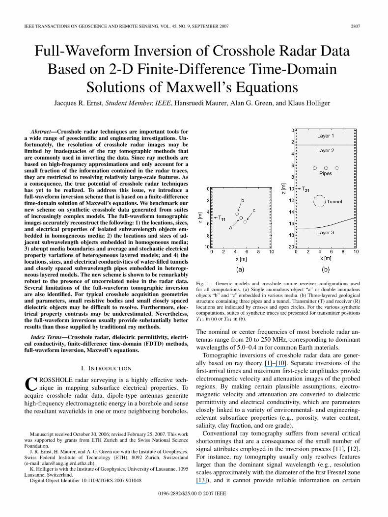
IEEE TRANSACTIONS ON GEOSCIENCE AND REMOTE SENSING, VOL. 45, NO. 9, SEPTEMBER 2007 2807 Full-Waveform Inversion of Crosshole Radar Data Based on 2-D Finite-Difference Time-Domain Solutions of Maxwell’s Equations Jacques R. Ernst, Student Member, IEEE, Hansruedi Maurer, Alan G. Green, and Klaus Holliger Abstract—Crosshole radar techniques are important tools for a wide range of geoscientific and engineering investigations. Un- fortunately, the resolution of crosshole radar images may be limited by inadequacies of the ray tomographic methods that are commonly used in inverting the data. Since ray methods are based on high-frequency approximations and only account for a small fraction of the information contained in the radar traces, they are restricted to resolving relatively large-scale features. As a consequence, the true potential of crosshole radar techniques has yet to be realized. To address this issue, we introduce a full-waveform inversion scheme that is based on a finite-difference time-domain solution of Maxwell’s equations. We benchmark our new scheme on synthetic crosshole data generated from suites of increasingly complex models. The full-waveform tomographic images accurately reconstruct the following: 1) the locations, sizes, and electrical properties of isolated subwavelength objects em- bedded in homogeneous media; 2) the locations and sizes of ad- jacent subwavelength objects embedded in homogeneous media; 3) abrupt media boundaries and average and stochastic electrical property variations of heterogeneous layered models; and 4) the locations, sizes, and electrical conductivities of water-filled tunnels and closely spaced subwavelength pipes embedded in heteroge- neous layered models. The new scheme is shown to be remarkably robust to the presence of uncorrelated noise in the radar data. Several limitations of the full-waveform tomographic inversion are also identified. For typical crosshole acquisition geometries and parameters, small resistive bodies and small closely spaced dielectric objects may be difficult to resolve. Furthermore, elec- trical property contrasts may be underestimated. Nevertheless, the full-waveform inversions usually provide substantially better results than those supplied by traditional ray methods. Index Terms—Crosshole radar, dielectric permittivity, electri- cal conductivity, finite-difference time-domain (FDTD) methods, full-waveform inversion, Maxwell’s equations. I. I NTRODUCTION C ROSSHOLE radar surveying is a highly effective tech- nique in mapping subsurface electrical properties. To acquire crosshole radar data, dipole-type antennas generate high-frequency electromagnetic energy in a borehole and sense the resultant wavefields in one or more neighboring boreholes. Manuscript received October 30, 2006; revised February 25, 2007. This work was supported by grants from ETH Zurich and the Swiss National Science Foundation. J. R. Ernst, H. Maurer, and A. G. Green are with the Institute of Geophysics, Swiss Federal Institute of Technology (ETH), 8092 Zurich, Switzerland (e-mail: [email protected]). K. Holliger is with the Institute of Geophysics, University of Lausanne, 1095 Lausanne, Switzerland. Digital Object Identifier 10.1109/TGRS.2007.901048 Fig. 1. Generic models and crosshole source–receiver configurations used for all computations. (a) Single anomalous object “a” or double anomalous objects “b” and “c” embedded in various media. (b) Three-layered geological structure containing three pipes and a tunnel. Transmitter (T) and receiver (R) locations are indicated by crosses and open circles. For the various synthetic computations, suites of synthetic traces are presented for transmitter positions T 11 in (a) or T 21 in (b). The nominal or center frequencies of most borehole radar an- tennas range from 20 to 250 MHz, corresponding to dominant wavelengths of 5.0–0.4 m for common Earth materials. Tomographic inversions of crosshole radar data are gener- ally based on ray theory [1]–[10]. Separate inversions of the first-arrival times and maximum first-cycle amplitudes provide electromagnetic velocity and attenuation images of the probed regions. By making certain plausible assumptions, electro- magnetic velocity and attenuation are converted to dielectric permittivity and electrical conductivity, which are parameters closely linked to a variety of environmental- and engineering- relevant subsurface properties (e.g., porosity, water content, salinity, clay fraction, and ore grade). Conventional ray tomography suffers from several critical shortcomings that are a consequence of the small number of signal attributes employed in the inversion process [11], [12]. For instance, ray tomography usually only resolves features larger than the dominant signal wavelength (e.g., resolution scales approximately with the diameter of the first Fresnel zone [13]), and it cannot provide reliable information on certain 0196-2892/$25.00 © 2007 IEEE
Transcript of Full-Waveform Inversion of Crosshole Radar Data Based on 2-D Finite-Difference Time-Domain Solutions...
IEEE TRANSACTIONS ON GEOSCIENCE AND REMOTE SENSING, VOL. 45, NO. 9, SEPTEMBER 2007 2807
Full-Waveform Inversion of Crosshole Radar DataBased on 2-D Finite-Difference Time-Domain
Solutions of Maxwell’s EquationsJacques R. Ernst, Student Member, IEEE, Hansruedi Maurer, Alan G. Green, and Klaus Holliger
Abstract—Crosshole radar techniques are important tools fora wide range of geoscientific and engineering investigations. Un-fortunately, the resolution of crosshole radar images may belimited by inadequacies of the ray tomographic methods thatare commonly used in inverting the data. Since ray methods arebased on high-frequency approximations and only account for asmall fraction of the information contained in the radar traces,they are restricted to resolving relatively large-scale features. Asa consequence, the true potential of crosshole radar techniqueshas yet to be realized. To address this issue, we introduce afull-waveform inversion scheme that is based on a finite-differencetime-domain solution of Maxwell’s equations. We benchmark ournew scheme on synthetic crosshole data generated from suitesof increasingly complex models. The full-waveform tomographicimages accurately reconstruct the following: 1) the locations, sizes,and electrical properties of isolated subwavelength objects em-bedded in homogeneous media; 2) the locations and sizes of ad-jacent subwavelength objects embedded in homogeneous media;3) abrupt media boundaries and average and stochastic electricalproperty variations of heterogeneous layered models; and 4) thelocations, sizes, and electrical conductivities of water-filled tunnelsand closely spaced subwavelength pipes embedded in heteroge-neous layered models. The new scheme is shown to be remarkablyrobust to the presence of uncorrelated noise in the radar data.Several limitations of the full-waveform tomographic inversionare also identified. For typical crosshole acquisition geometriesand parameters, small resistive bodies and small closely spaceddielectric objects may be difficult to resolve. Furthermore, elec-trical property contrasts may be underestimated. Nevertheless,the full-waveform inversions usually provide substantially betterresults than those supplied by traditional ray methods.
Index Terms—Crosshole radar, dielectric permittivity, electri-cal conductivity, finite-difference time-domain (FDTD) methods,full-waveform inversion, Maxwell’s equations.
I. INTRODUCTION
CROSSHOLE radar surveying is a highly effective tech-nique in mapping subsurface electrical properties. To
acquire crosshole radar data, dipole-type antennas generatehigh-frequency electromagnetic energy in a borehole and sensethe resultant wavefields in one or more neighboring boreholes.
Manuscript received October 30, 2006; revised February 25, 2007. This workwas supported by grants from ETH Zurich and the Swiss National ScienceFoundation.
J. R. Ernst, H. Maurer, and A. G. Green are with the Institute of Geophysics,Swiss Federal Institute of Technology (ETH), 8092 Zurich, Switzerland(e-mail: [email protected]).
K. Holliger is with the Institute of Geophysics, University of Lausanne, 1095Lausanne, Switzerland.
Digital Object Identifier 10.1109/TGRS.2007.901048
Fig. 1. Generic models and crosshole source–receiver configurations usedfor all computations. (a) Single anomalous object “a” or double anomalousobjects “b” and “c” embedded in various media. (b) Three-layered geologicalstructure containing three pipes and a tunnel. Transmitter (T) and receiver (R)locations are indicated by crosses and open circles. For the various syntheticcomputations, suites of synthetic traces are presented for transmitter positionsT11 in (a) or T21 in (b).
The nominal or center frequencies of most borehole radar an-tennas range from 20 to 250 MHz, corresponding to dominantwavelengths of 5.0–0.4 m for common Earth materials.
Tomographic inversions of crosshole radar data are gener-ally based on ray theory [1]–[10]. Separate inversions of thefirst-arrival times and maximum first-cycle amplitudes provideelectromagnetic velocity and attenuation images of the probedregions. By making certain plausible assumptions, electro-magnetic velocity and attenuation are converted to dielectricpermittivity and electrical conductivity, which are parametersclosely linked to a variety of environmental- and engineering-relevant subsurface properties (e.g., porosity, water content,salinity, clay fraction, and ore grade).
Conventional ray tomography suffers from several criticalshortcomings that are a consequence of the small number ofsignal attributes employed in the inversion process [11], [12].For instance, ray tomography usually only resolves featureslarger than the dominant signal wavelength (e.g., resolutionscales approximately with the diameter of the first Fresnel zone[13]), and it cannot provide reliable information on certain
0196-2892/$25.00 © 2007 IEEE

2808 IEEE TRANSACTIONS ON GEOSCIENCE AND REMOTE SENSING, VOL. 45, NO. 9, SEPTEMBER 2007
TABLE IMODEL PARAMETERS. HOMOGENEOUS MODELS WERE USED AS INPUTS
FOR ALL RAY TOMOGRAPHIC INVERSIONS. THE RELATIVE
PERMITTIVITIES AND CONDUCTIVITIES OF THESE
MODELS ARE PROVIDED IN THE LAST COLUMN
important types of low-velocity structures. These deficienciesare particularly acute for targets that can only be illuminatedfrom a limited number of directions, which is the situation formany crosshole investigations.
Since inversion is important for a wide range of problems inseismic exploration and exploitation, medical imaging, nonde-structive testing, and tunnel and landmine detection, a numberof accurate alternative methods for inverting diverse types ofwavefield data (e.g., acoustic, elastic, radar, microwave, optical,and X-ray) have evolved over the past two decades. As ex-amples, the following waveform-based tomographic inversionmethods have been introduced in exploration seismology:
1) Fresnel volume [14], [15];2) wave-equation traveltime [16]–[19];3) diffraction [20]–[25];4) full-waveform [26]–[47].
These methods have been developed for both acoustic andelastic waves generated and recorded at the surface and/or alongboreholes. They have included finite-difference and finite-element approaches in both the time- and frequency-domains.
In exploration seismology, waveform-based inversionschemes provide subwavelength resolution [37], and underfavorable conditions, the resolution is as good as one-half[21] to one-third [24] of a wavelength. In a direct comparison,Dessa and Pascal [47] demonstrate that waveform-basedinversion of ultrasonic data improves the resolution thresholdby an order-of-magnitude relative to that supplied by ray
tomography. By considering information contained in relevantparts of the entire recorded signal, waveform-based inversionsare capable of providing reliable information on a broad rangeof structures, including those distinguished by low velocities.
Advances in waveform-based tomographic inversions ofradar data have either been made as a result of indepen-dent developments in electromagnetism or implicitly/explicitlyfollowed those made in exploration seismology (i.e., theacoustic/elastic equations have been replaced by Maxwell’sequations, and the solutions have been appropriately refor-mulated). Important advances in the first category resultedfrom various Born iterative methods based on integral rep-resentations of Maxwell’s equations [48]–[54]. In the secondcategory, Johnson et al. [55] and Cai et al. [56] adaptedthe Fresnel volume and wave-equation traveltime methods,respectively, and different authors [57]–[63] reported modi-fied diffraction tomography techniques. An early attempt byMoghaddam et al. [51] to determine the dielectric permittivitiesof small objects from synthetic data using a suitably modifiedversion of Tarantola’s [26], [27] full-waveform inversion ap-proach was not considered fully satisfactory by the authors,primarily because significant a priori information was requiredto ensure correct convergence. We have since learned fromnumerous studies in seismology that a good initial model isrequired for the successful application of many full-waveformtomographic inversion techniques (e.g., see review by Dessaand Pascal [47]). Independently, three groups have recentlydeveloped full-waveform time-domain tomographic inversionschemes and tested them on synthetic radar data [64]–[66]. Allthree groups were able to determine the locations and relativepermittivities of subwavelength bodies located within weaklyconductive media.
Despite the considerable advantages compared to ray to-mography, most applications of waveform-based inversiontechniques to synthetic and observed crosshole radar datahave suffered from one or more of the following limitations:1) unrealistic assumptions were made about the backgroundmedia (e.g., they were assumed to be homogeneous and/orlossless); 2) the effects of realistic electrical conductivities wereignored; 3) the conductivities were not determined; 4) onlylow contrasts between the target structures and backgroundmedium were accommodated (e.g., they were based on the Bornor Rytov weak scattering approximations); 5) only one or afew discrete targets were imaged; 6) target shapes had to beknown; 7) target sizes had to be large relative to the dominantwavelength of the signal; and/or 8) monofrequency signals wereemployed.
In this contribution, we describe a full-waveform time-domain tomographic inversion scheme for crosshole radar data.It provides high-resolution dielectric permittivity and electricalconductivity images of the Earth between boreholes by auto-matically accounting for all phases of the radar signal. Thebackground media may be heterogeneous, the physical propertycontrasts are not limited by the Born or Rytov weak scatter-ing approximations, and the size of the dielectric/conductivetargets may be smaller than the dominant wavelength of theradar signal. As for other full-waveform inversion methods, agood initial model is required to prevent the inversion process

ERNST et al.: INVERSION OF RADAR DATA BASED ON FDTD SOLUTIONS OF MAXWELL’S EQUATIONS 2809
Fig. 2. Relative permittivity (εr) tomograms and cross sections derived from synthetic radar traces generated for input model 1 (Table I) with a medium relativepermittivity εrm = 4.0 and a medium conductivity σm = 0.1 mS/m, and a single small object [a in Fig. 1(a)] with εra = 5.0 and σa = 0.1 mS/m. (a) and (b) To-mograms that result from applying ray-based and full-waveform inversion schemes to noise-free synthetic radar traces. Dashed white circles delineate the object’strue location. (c) Blue, red, and black lines are the A cross sections through the tomograms in (a) and (b) and input model. (d) As for (c), but for the B cross sections.(e) and (f) Tomograms that result from applying the full-waveform inversion scheme to synthetic radar traces contaminated with 5% and 20% random noises.(g) Blue, red, and black lines are the A cross sections through the tomograms in (e) and (f) and input model. (h) As for (g), but for the B cross sections.
converging to local minima in the search space. Accordingly,we employ conventional ray tomography to derive the initialmodels [37], [39], [42], [47].
After presenting the theory for the forward and inversecomponents of our new scheme, key implementation issues arehighlighted. We then illustrate the advantages and limitations
2810 IEEE TRANSACTIONS ON GEOSCIENCE AND REMOTE SENSING, VOL. 45, NO. 9, SEPTEMBER 2007
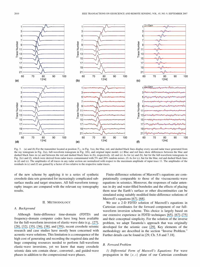
Fig. 3. (a) and (b) For the transmitter located at position T11 in Fig. 1(a), the blue, red, and dashed black lines display every second radar trace generated fromthe ray tomogram in Fig. 2(a), full-waveform tomogram in Fig. 2(b), and original input model. (c) Blue and red lines show differences between the blue anddashed black lines in (a) and between the red and dashed black lines in (b), respectively. (d) and (e) As for (a) and (b), but for the full-waveform tomograms inFig. 2(e) and (f), which were derived from radar traces contaminated with 5% and 20% random noises. (f) As for (c), but for the blue, red and dashed black linesin (d) and (e). The amplitudes of all traces in any radar section are normalized with respect to the maximum amplitude of input trace 11. The amplitudes of theresiduals in (c) and (f) are gained by a factor of two relative to the respective radar traces.
of the new scheme by applying it to a series of syntheticcrosshole data sets generated for increasingly complicated sub-surface media and target structures. All full-waveform tomog-raphy images are compared with the relevant ray tomographyresults.
II. METHODOLOGY
A. Background
Although finite-difference time-domain (FDTD) andfrequency-domain computer codes have long been availablefor the full-waveform inversion of elastic-wave data (e.g., [27],[28], [32], [35], [36], [38], and [39]), recent crosshole seismicresearch and case studies have mostly been concerned withacoustic-wave solutions. This limitation is a consequence of thehigh cost of generating and recording the required data and thehuge computing resources needed to perform full-waveformelastic-wave inversions, yet we know that many crossholeseismic data sets contain shear-, converted-, and guided-wavephases in addition to the compressional-wave phases.
Finite-difference solutions of Maxwell’s equations are com-putationally comparable to those of the viscoacoustic-waveequations in seismics. Moreover, the responses of radar anten-nas in dry and water-filled boreholes and the effects of placingthem near the Earth’s surface or other discontinuities can besimulated using suitably modified finite-difference solutions ofMaxwell’s equations [67], [68].
We use a 2-D FDTD solution of Maxwell’s equations inCartesian coordinates for the forward component of our full-waveform inversion scheme. This choice is largely based onour extensive experience in FDTD techniques [65], [67]–[75]and their conceptual simplicity. For the solution of the inverseproblem, we adapt Tarantola’s approach that was originallydeveloped for the seismic case [29]. Key elements of themethodology are described in the section “Inverse Problem.”Further details can be found in [29, Ch. 5.8 and 7.18].
B. Forward Problem
1) Differential Form of Maxwell’s Equations: For wavepropagation in the (x, z) plane of our Cartesian coordinate

ERNST et al.: INVERSION OF RADAR DATA BASED ON FDTD SOLUTIONS OF MAXWELL’S EQUATIONS 2811
Fig. 4. Conductivity (σ) tomograms and cross sections derived from synthetic radar traces generated for input model 2 (Table I) with a medium relativepermittivity εrm = 4 and a medium conductivity σm = 0.1 mS/m, and a single small object [a in Fig. 1(a)] with εra = 4 and σa = 10.0 mS/m. All other detailsare explained in Fig. 2.
system, the transverse electric or TE mode of Maxwell’s equa-tions can be written as [76]
∂Ex
∂t=
1ε
(−∂Hy
∂z− σEx
)(1a)
∂Ez
∂t=
1ε
(∂Hy
∂x− σEz
)(1b)
∂Hy
∂t=
1µ
(∂Ez
∂x− ∂Ex
∂z
)(1c)

2812 IEEE TRANSACTIONS ON GEOSCIENCE AND REMOTE SENSING, VOL. 45, NO. 9, SEPTEMBER 2007
Fig. 5. As for Fig. 3, but showing radar sections and residuals for the inversion results illustrated in Fig. 4. The amplitudes of the residuals in (c) and (f) aregained by factors of eight and two relative to the respective radar traces.
where Ex and Ez are the horizontal and vertical electric fieldcomponents, Hy is the magnetic field perpendicular to thepropagation plane, ε is the dielectric permittivity, σ is theelectrical conductivity, and µ is the magnetic permeability(assumed in the following to be constant and equal to thefree-space permeability µ0 ). Bold letters are used to representvectors and matrices. Equations (1a)–(1c) can be solved effi-ciently using FDTD techniques (e.g., [76] and [77]) based onstaggered-grid finite-difference operators that are second-orderaccurate in both space and time. Highly efficient generalizedperfectly matched layer (GPML) absorbing boundaries [78],[79] minimize the artificial reflections at the edges of themodel space.
2) Integral Form of Maxwell’s Equations: To determinethe update directions required in our inversion procedure,it is useful to work with the integral form of Maxwell’sequations. Typical borehole radar systems record the verticalcomponent of the electric field Ez , such that Maxwell’s equa-tions can be recast in a form corresponding to the telegraphyequation
ε∂2Ez
∂t2− 1
µ
∂2Ez
∂x2+ σ
∂Ez
∂t= Ψz (2)
where x is a vector that refers to location (x, z), and Ψz isthe source function. Solutions of (2) can be formally expressedusing Green’s functions Gz [80]
Ez(x, t) =∫V
dV(x′)
Tmax∫0
dt′Gz(x, t;x′, t′)Ψz(x′, t′) (3)
where V is the model space and Tmax is the maximum obser-vation time.
C. Inverse Problem
1) Inversion Strategy: Our full-waveform tomographic in-version scheme for crosshole radar data involves finding thespatial distributions of ε and σ that minimize a functional ofthe form
S =12‖Ez (xtrn,xrec, t, ε(x),σ(x))
−Eobsz (xtrn,xrec, t, εtrue(x),σtrue(x))
∥∥2(4)

ERNST et al.: INVERSION OF RADAR DATA BASED ON FDTD SOLUTIONS OF MAXWELL’S EQUATIONS 2813
Fig. 6. Relative permittivity (ε) and conductivity (σ) tomograms and cross sections derived from synthetic radar traces generated for input model 3 (Table I) witha medium relative permittivity εrm = 4.0 and a medium conductivity σm = 3.0 mS/m, and two small objects [b and c in Fig. 1(a)], the upper with εrb = 5.0and σb = 10.0 mS/m and the lower with εrc = 3.0 and σc = 0.1 mS/m. (a) and (d) εr and σ tomograms that result from applying the ray-based inversionscheme to noise-free synthetic radar traces. (b) and (e) As for (a) and (d), but showing the results of applying the full-waveform inversion scheme to radar tracescontaminated with 5% random noise. (c) Blue, red, and black lines are diagonal cross sections C through the tomograms in (a) and (b) and input model. (f) Blue,red, and black lines are diagonal cross sections C through the tomograms in (d) and (e) and input model. Dashed white circles in (a), (b), (d), and (e) delineate theobjects’ true locations.
where xtrn and xrec are vectors that identify the transmitterand receiver positions, ε and σ are the model permittivityand conductivity distributions, and εtrue and σtrue are thetrue subsurface parameters. Ez and Eobs
z are the synthetic(computed) and observed vertical electric fields at the receiver
locations. Following Tarantola [29], we use logarithmicallyscaled versions of our unknown parameters
ε=log(
ε
ε0
)=log(εr) and σ= log
(σ
σ0
)= log (σ) (5)
2814 IEEE TRANSACTIONS ON GEOSCIENCE AND REMOTE SENSING, VOL. 45, NO. 9, SEPTEMBER 2007
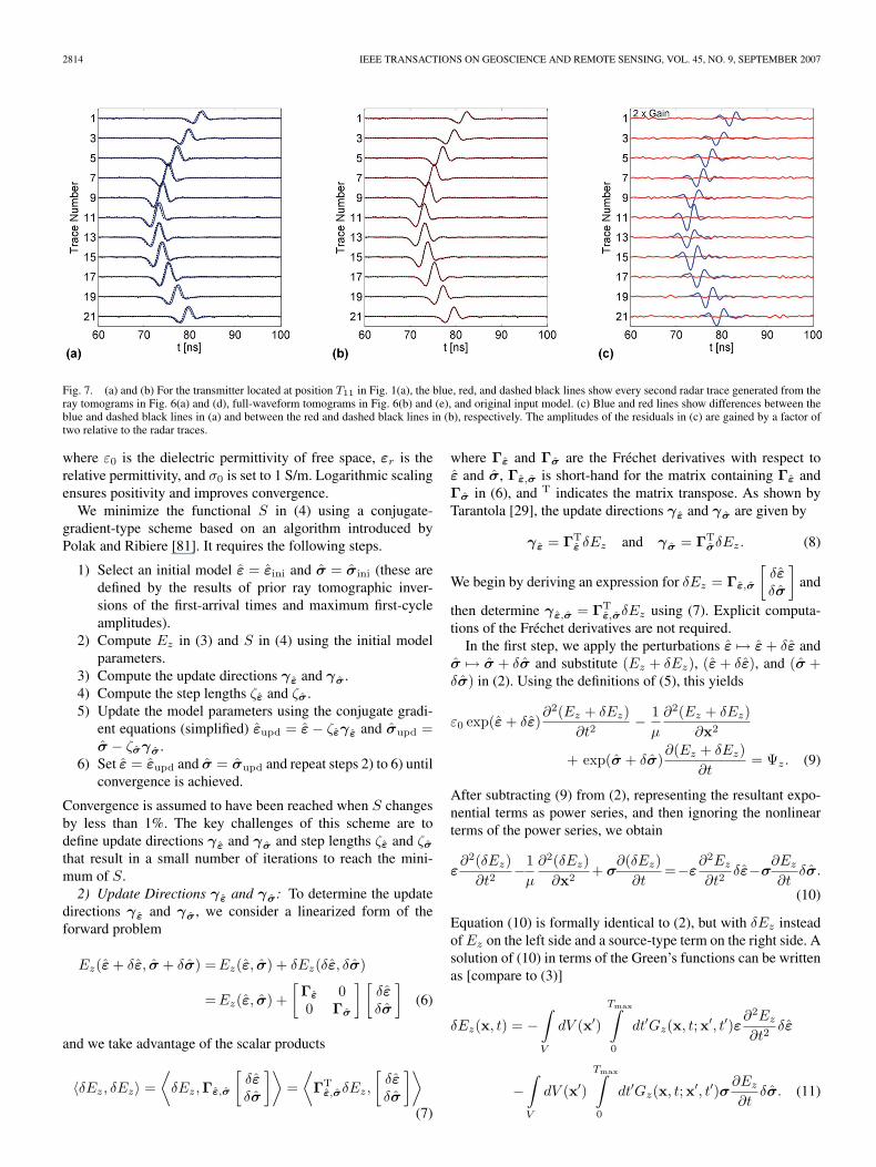
Fig. 7. (a) and (b) For the transmitter located at position T11 in Fig. 1(a), the blue, red, and dashed black lines show every second radar trace generated from theray tomograms in Fig. 6(a) and (d), full-waveform tomograms in Fig. 6(b) and (e), and original input model. (c) Blue and red lines show differences between theblue and dashed black lines in (a) and between the red and dashed black lines in (b), respectively. The amplitudes of the residuals in (c) are gained by a factor oftwo relative to the radar traces.
where ε0 is the dielectric permittivity of free space, εr is therelative permittivity, and σ0 is set to 1 S/m. Logarithmic scalingensures positivity and improves convergence.
We minimize the functional S in (4) using a conjugate-gradient-type scheme based on an algorithm introduced byPolak and Ribiere [81]. It requires the following steps.
1) Select an initial model ε = εini and σ = σini (these aredefined by the results of prior ray tomographic inver-sions of the first-arrival times and maximum first-cycleamplitudes).
2) Compute Ez in (3) and S in (4) using the initial modelparameters.
3) Compute the update directions γ ε and γσ .4) Compute the step lengths ζε and ζσ .5) Update the model parameters using the conjugate gradi-
ent equations (simplified) εupd = ε − ζεγ ε and σupd =σ − ζσγσ.
6) Set ε = εupd and σ = σupd and repeat steps 2) to 6) untilconvergence is achieved.
Convergence is assumed to have been reached when S changesby less than 1%. The key challenges of this scheme are todefine update directions γ ε and γσ and step lengths ζε and ζσ
that result in a small number of iterations to reach the mini-mum of S.
2) Update Directions γ ε and γσ: To determine the updatedirections γ ε and γσ , we consider a linearized form of theforward problem
Ez(ε + δε, σ + δσ) =Ez(ε, σ) + δEz(δε, δσ)
=Ez(ε, σ) +[Γε 00 Γσ
] [δεδσ
](6)
and we take advantage of the scalar products
〈δEz, δEz〉 =⟨
δEz,Γε,σ
[δεδσ
]⟩=
⟨ΓT
ε,σδEz,
[δεδσ
]⟩(7)
where Γε and Γσ are the Fréchet derivatives with respect toε and σ, Γε,σ is short-hand for the matrix containing Γε andΓσ in (6), and T indicates the matrix transpose. As shown byTarantola [29], the update directions γ ε and γσ are given by
γ ε = ΓTε δEz and γσ = ΓT
σδEz. (8)
We begin by deriving an expression for δEz = Γε,σ
[δεδσ
]and
then determine γ ε,σ = ΓTε,σδEz using (7). Explicit computa-
tions of the Fréchet derivatives are not required.In the first step, we apply the perturbations ε �→ ε + δε and
σ �→ σ + δσ and substitute (Ez + δEz), (ε + δε), and (σ +δσ) in (2). Using the definitions of (5), this yields
ε0 exp(ε + δε)∂2(Ez + δEz)
∂t2− 1
µ
∂2(Ez + δEz)∂x2
+ exp(σ + δσ)∂(Ez + δEz)
∂t= Ψz. (9)
After subtracting (9) from (2), representing the resultant expo-nential terms as power series, and then ignoring the nonlinearterms of the power series, we obtain
ε∂2(δEz)
∂t2−1
µ
∂2(δEz)∂x2
+ σ∂(δEz)
∂t=−ε
∂2Ez
∂t2δε−σ
∂Ez
∂tδσ.
(10)
Equation (10) is formally identical to (2), but with δEz insteadof Ez on the left side and a source-type term on the right side. Asolution of (10) in terms of the Green’s functions can be writtenas [compare to (3)]
δEz(x, t) = −∫V
dV (x′)
Tmax∫0
dt′Gz(x, t;x′, t′)ε∂2Ez
∂t2δε
−∫V
dV (x′)
Tmax∫0
dt′Gz(x, t;x′, t′)σ∂Ez
∂tδσ. (11)

ERNST et al.: INVERSION OF RADAR DATA BASED ON FDTD SOLUTIONS OF MAXWELL’S EQUATIONS 2815
Fig. 8. (a) and (d) Input εr and σ values for model 4 (as for Fig. 1(b), but without the pipes and tunnel; Table I). Parameters of the three layers are the following:εr1 = 5.2 and σ1 = 2.8 mS/m, εr2 = 3.7 and σ2 = 2.0 mS/m, and εr3 = 5.0 and σ3 = 0.1 mS/m. (b) and (e) εr and σ tomograms that result from applyingthe ray-based inversion scheme to noise-free synthetic radar traces generated from model 4. (c) and (f) As for (b) and (e), but for the results of the full-waveforminversions.
In the second step, we consider the integral representationsof the scalar products on the left and right sides of (7)
〈δEz, δEz〉 =∑trn
Tmax∫0
dt∑rec
δEzδEz (12)
and
⟨[ΓT
ε δEz
ΓTσδEz
],
[δεδσ
]⟩=
∫V
dV(ΓT
ε δEz · δε)
+∫V
dV(ΓT
σδEz · δσ). (13)
By substituting (11) in (12), the integral representation of (7)becomes
∑trn
Tmax∫0
dt∑rec
δEz
−∫
V
dV
Tmax∫0
dt′Gzε∂2Ez
∂t2δε
−∫V
dV
Tmax∫0
dt′Gzσ∂Ez
∂tδσ
=∫V
dV(ΓT
ε δEz · δε)
+∫V
dV(ΓT
σδEz · δσ). (14)
Since (14) is valid for arbitrary small values of δε and δσ,we can equate the terms containing permittivity and the terms
2816 IEEE TRANSACTIONS ON GEOSCIENCE AND REMOTE SENSING, VOL. 45, NO. 9, SEPTEMBER 2007
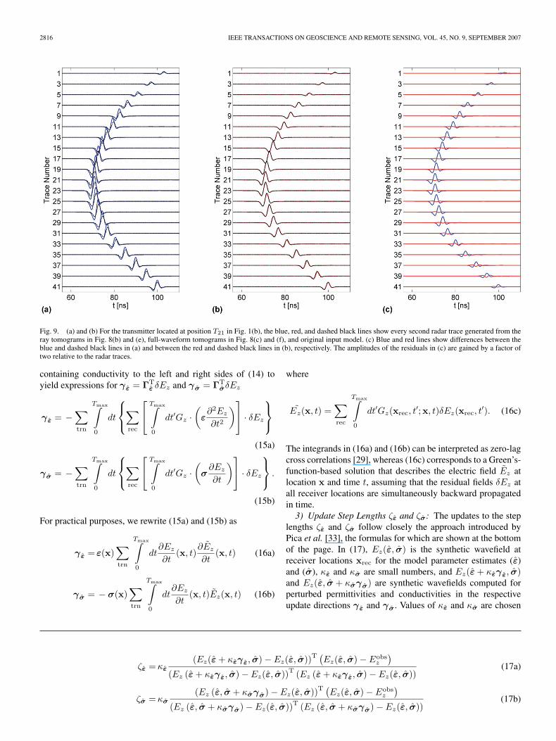
Fig. 9. (a) and (b) For the transmitter located at position T21 in Fig. 1(b), the blue, red, and dashed black lines show every second radar trace generated from theray tomograms in Fig. 8(b) and (e), full-waveform tomograms in Fig. 8(c) and (f), and original input model. (c) Blue and red lines show differences between theblue and dashed black lines in (a) and between the red and dashed black lines in (b), respectively. The amplitudes of the residuals in (c) are gained by a factor oftwo relative to the radar traces.
containing conductivity to the left and right sides of (14) toyield expressions for γ ε = ΓT
ε δEz and γσ = ΓTσδEz
γ ε = −∑trn
Tmax∫0
dt
∑rec
Tmax∫
0
dt′Gz ·(
ε∂2Ez
∂t2
) · δEz
(15a)
γσ = −∑trn
Tmax∫0
dt
∑rec
Tmax∫
0
dt′Gz ·(
σ∂Ez
∂t
) · δEz
.
(15b)
For practical purposes, we rewrite (15a) and (15b) as
γ ε = ε(x)∑trn
Tmax∫0
dt∂Ez
∂t(x, t)
∂Ez
∂t(x, t) (16a)
γσ = − σ(x)∑trn
Tmax∫0
dt∂Ez
∂t(x, t)Ez(x, t) (16b)
where
Ez(x, t) =∑rec
Tmax∫0
dt′Gz(xrec, t′;x, t)δEz(xrec, t
′). (16c)
The integrands in (16a) and (16b) can be interpreted as zero-lagcross correlations [29], whereas (16c) corresponds to a Green’s-function-based solution that describes the electric field Ez atlocation x and time t, assuming that the residual fields δEz atall receiver locations are simultaneously backward propagatedin time.
3) Update Step Lengths ζε and ζσ: The updates to the steplengths ζε and ζσ follow closely the approach introduced byPica et al. [33], the formulas for which are shown at the bottomof the page. In (17), Ez(ε, σ) is the synthetic wavefield atreceiver locations xrec for the model parameter estimates (ε)and (σ), κε and κσ are small numbers, and Ez(ε + κεγ ε, σ)and Ez(ε, σ + κσγσ) are synthetic wavefields computed forperturbed permittivities and conductivities in the respectiveupdate directions γ ε and γσ . Values of κε and κσ are chosen
ζε = κε
(Ez(ε + κεγ ε, σ) − Ez(ε, σ))T(Ez(ε, σ) − Eobs
z
)(Ez (ε + κεγ ε, σ) − Ez(ε, σ))T (Ez (ε + κεγ ε, σ) − Ez(ε, σ))
(17a)
ζσ = κσ
(Ez (ε, σ + κσγσ) − Ez(ε, σ))T(Ez(ε, σ) − Eobs
z
)(Ez (ε, σ + κσγσ) − Ez(ε, σ))T (Ez (ε, σ + κσγσ) − Ez(ε, σ))
(17b)
ERNST et al.: INVERSION OF RADAR DATA BASED ON FDTD SOLUTIONS OF MAXWELL’S EQUATIONS 2817
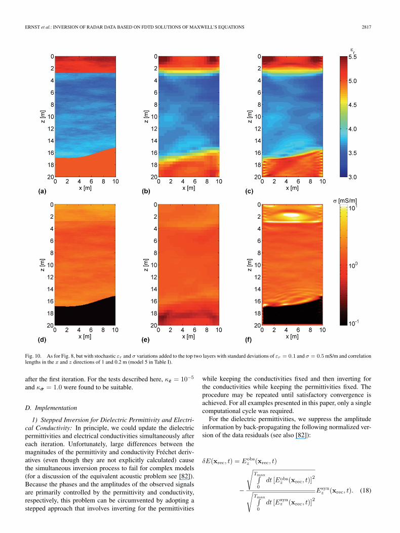
Fig. 10. As for Fig. 8, but with stochastic εr and σ variations added to the top two layers with standard deviations of εr = 0.1 and σ = 0.5 mS/m and correlationlengths in the x and z directions of 1 and 0.2 m (model 5 in Table I).
after the first iteration. For the tests described here, κε = 10−5
and κσ = 1.0 were found to be suitable.
D. Implementation
1) Stepped Inversion for Dielectric Permittivity and Electri-cal Conductivity: In principle, we could update the dielectricpermittivities and electrical conductivities simultaneously aftereach iteration. Unfortunately, large differences between themagnitudes of the permittivity and conductivity Fréchet deriv-atives (even though they are not explicitly calculated) causethe simultaneous inversion process to fail for complex models(for a discussion of the equivalent acoustic problem see [82]).Because the phases and the amplitudes of the observed signalsare primarily controlled by the permittivity and conductivity,respectively, this problem can be circumvented by adopting astepped approach that involves inverting for the permittivities
while keeping the conductivities fixed and then inverting forthe conductivities while keeping the permittivities fixed. Theprocedure may be repeated until satisfactory convergence isachieved. For all examples presented in this paper, only a singlecomputational cycle was required.
For the dielectric permittivities, we suppress the amplitudeinformation by back-propagating the following normalized ver-sion of the data residuals (see also [82]):
δE(xrec, t) = Eobsz (xrec, t)
−
√Tmax∫0
dt [Eobsz (xrec, t)]
2
√Tmax∫0
dt [Esynz (xrec, t)]
2
Esynz (xrec, t). (18)

2818 IEEE TRANSACTIONS ON GEOSCIENCE AND REMOTE SENSING, VOL. 45, NO. 9, SEPTEMBER 2007
Fig. 11. As for Fig. 9, but for the tomograms in Fig. 10.
By including realistic conductivities in the input model (e.g.,those obtained with ray amplitude inversion), we partly accountfor the effects of electrical conductivity on the phases (e.g.,[56]). After determining the distribution of permittivities, theoriginal data are used for the conductivity inversion, i.e., thenormalization terms in (18) are not applied.
2) Computational Issues: Our full-waveform inversionscheme requires the forward problem to be solved three timesper iteration for each transmitter location: once to evaluatethe synthetic data Ez [step 2) of our implementation of Polakand Ribiere’s [81] algorithm], once to compute the updatedirections [step 3); eq. (16)], and once to determine the steplength [step 4); eq. (17)]. Consequently, the computationalcosts of forward modeling largely control the efficiency of ourwaveform inversion scheme.
By using FDTD techniques to solve the forward problem fora typical crosshole radar data set requires 105–106 grid pointsand a few tens of transmitter positions, for which a few thou-sand time steps need to be computed. For computation of theupdate directions (16), the complete Ez fields generated by alltransmitters at all grid locations need to be kept in memory. Thiswould require a large core memory of about 20 × Ntrn GigaBytes, where Ntrn is the number of transmitters. However, thespatial resolution of the data is much lower than the discretiza-tion needed for accurate forward modeling, so that a number offorward modeling cells can be represented with a single inver-sion cell. We include 3 × 3 forward modeling cells within oneinversion cell without loss of resolution in the inversion process.This reduces the memory requirements by roughly an orderof magnitude, thus making the computations tractable with-out having to implement time-consuming memory-swappingprocedures. Furthermore, because the single transmitter cal-culations are largely independent of each other, the computa-tional scheme can be implemented efficiently on a distributed
computer network comprising one CPU per transmitter plus amaster CPU. The overhead for distributing the computationsis only about 10%. Accordingly, the total computational timeTcomp required for a complete inversion is given by
Tcomp ≈ 3 · 1.1 · Tforward · Niter (19)
where Tforward is the time required for a single forward calcula-tion, and Niter is the number of iterations. On a PC cluster con-sisting of Opteron 244 processors, each with 4-GB of memory,the computational time for a single-parameter inversion with105 forward grid points requires 3 h, whereas that for a two-parameter inversion with 106 forward grid points requires 18 h.
III. APPLICATIONS TO SYNTHETIC DATA
We explore the potential and limitations of our full-waveformtomographic inversion scheme using synthetic data generatedfrom a suite of increasingly complex models. The modelsand acquisition geometries are shown in Fig. 1, and the keyparameters are summarized in Table I. For the first three nu-merical experiments [Fig. 1(a)], two 10-m-deep boreholes areseparated by 10 m, and the forward and inverse grids havespacings of 0.02 and 0.06 m, respectively. There are 21 equallyspaced transmitter antenna locations in the left borehole and 21equally spaced receiver antenna locations in the right borehole.The model space is surrounded by a 0.8-m-thick GPML frame.For the other experiments [Fig. 1(b)], the borehole depthsare increased to 20 m, and the number of transmitters andreceivers are increased to 41. All other acquisition parametersare identical to those of the first three experiments.
We employed the same FDTD code to create the syntheticdata and to solve the forward problems in the inversion process.The waveform of the source signal corresponded to a Gaussian

ERNST et al.: INVERSION OF RADAR DATA BASED ON FDTD SOLUTIONS OF MAXWELL’S EQUATIONS 2819
Fig. 12. As for Fig. 8, but with stochastic εr and σ variations added to the top two layers with standard deviations of εr = 0.3 and σ = 1.5 mS/m and correlationlengths in the x and z directions of 1 and 0.2 m (model 6 in Table I).
pulse with a nominal frequency of ∼150 MHz and a bandwidthof ∼3 octaves, which yielded a dominant wavelength of ∼1 min our models.
To begin the inversion process, we applied conventionalray tomography using the first-arrival times and maximumfirst-cycle amplitudes [4], [6], [9] to obtain the velocity andattenuation tomograms that were converted to correspondingdielectric permittivity and electrical conductivity distributionsusing the following high-frequency approximations:
ε ≈ 1µ0
ν−2 (20a)
and
σ ≈ 2α
√ε
µ0(20b)
where ν and α are velocity and attenuation, respectively. Theresulting ε and σ distributions (our optimum ray tomograms)were then used as the initial models for the full-waveformtomographic inversions. The ε and σ computations usually con-verged after 20 and 10 iterations, respectively. For convenience,we describe our models in the following in terms of the relativepermittivity εr = ε/ε0. Initial εr and σ values (converted tocorresponding velocities and attenuations) that are used to startthe ray tomographic inversions are shown in the last columnof Table I.
A. Numerical Experiment 1: Single Dielectric Object in aHomogeneous Medium
Model 1 comprises a high-permittivity circular object (a inFig. 1(a); εra = 5.0) embedded in the center of a homogeneousmedium (εra = 4.0). The diameter of the anomalous object is
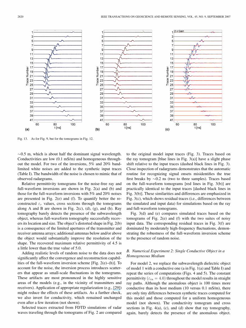
2820 IEEE TRANSACTIONS ON GEOSCIENCE AND REMOTE SENSING, VOL. 45, NO. 9, SEPTEMBER 2007
Fig. 13. As for Fig. 9, but for the tomograms in Fig. 12.
∼0.5 m, which is about half the dominant signal wavelength.Conductivities are low (0.1 mS/m) and homogeneous through-out the model. For two of the inversions, 5% and 20% band-limited white noises are added to the synthetic input traces(Table I). The bandwidth of the noise is chosen to mimic that ofobserved radargrams.
Relative permittivity tomograms for the noise-free ray andfull-waveform inversions are shown in Fig. 2(a) and (b) andthose for the full-waveform inversions with 5% and 20% noisesare presented in Fig. 2(e) and (f). To quantify better the re-constructed εr values, cross sections through the tomogramsalong A and B are shown in Fig. 2(c), (d), (g), and (h). Raytomography barely detects the presence of the subwavelengthobject, whereas full-waveform tomography successfully recov-ers its location and size. The object’s distorted shape in Fig. 2(b)is a consequence of the limited apertures of the transmitter andreceiver antenna arrays; additional antennas below and/or abovethe object would substantially improve the resolution of theshape. The recovered maximum relative permittivity of 4.5 isa little lower than the true value of 5.0.
Adding realistic levels of random noise to the data does notsignificantly affect the convergence and reconstruction capabil-ities of the full-waveform inversion scheme [Fig. 2(e)–(h)]. Toaccount for the noise, the inversion process introduces scatter-ers that appear as small-scale fluctuations in the tomograms.These artifacts are most pronounced in the highly sensitiveareas of the models (e.g., in the vicinity of transmitters andreceivers). Application of appropriate regularization (e.g., [29])might reduce the effects of these artifacts. As a further check,we also invert for conductivity, which remained unchangedeven after a few iteration (not shown).
Selected traces extracted from FDTD simulations of radarwaves traveling through the tomograms of Fig. 2 are compared
to the original model input traces (Fig. 3). Traces based onthe ray tomogram [blue lines in Fig. 3(a)] have a slight phaseshift relative to the input traces (dashed black lines in Fig. 3).Close inspection of radargrams demonstrates that the automaticroutine for recognizing signal onsets misidentifies the truefirst breaks by ∼0.2 ns (two to three samples). Traces basedon the full-waveform tomograms [red lines in Fig. 3(b)] arepractically identical to the input traces [dashed black lines inFig. 3(b)]. These similarities and differences are emphasized inFig. 3(c), which shows residual traces (i.e., differences betweenthe simulated and input data) for simulations based on the rayand full-waveform tomograms.
Fig. 3(d) and (e) compares simulated traces based on thetomograms of Fig. 2(e) and (f) with the two suites of noisyinput data. The corresponding residual traces in Fig. 3(f) aredominated by moderately high-frequency fluctuations, demon-strating the robustness of the full-waveform inversion schemeto the presence of random noise.
B. Numerical Experiment 2: Single Conductive Object in aHomogeneous Medium
For model 2, we replace the subwavelength dielectric objectof model 1 with a conductive one (a in Fig. 1(a) and Table I) andrepeat the series of computations (Figs. 4 and 5). The constantpermittivity (εra = 4.0) throughout the model results in straightray paths. Although the anomalous object is 100 times moreconductive than its host medium (10 versus 0.1 mS/m), thereare only tiny differences between synthetic traces computed forthis model and those computed for a uniform homogeneousmodel (not shown). The conductivity tomogram and crosssections in Fig. 4(a), (c), and (d) show that ray tomography,again, barely detects the presence of the anomalous object.

ERNST et al.: INVERSION OF RADAR DATA BASED ON FDTD SOLUTIONS OF MAXWELL’S EQUATIONS 2821
Fig. 14. As for Fig. 8, but with the addition of three pipes and a tunnel filled with moderately conductive water [Fig. 1(b); model 7 in Table I]. For the pipes andtunnel, εrp = εrt = 80, and σp = σt = 10.0 mS/m.
By comparison, the anomaly’s location, size, and conductivityare satisfactorily reproduced in the full-waveform tomograms,even in those based on the noisy traces [Fig. 4(b)–(h)]. As innumerical experiment 1, the shape of the reconstructed objectis somewhat distorted.
Since we are primarily interested in the role played byconductivity in this experiment, we use the correct constantpermittivity in simulating traces based on the conductivity raytomogram of Fig. 5(a) (note the absence of an anomalous phaseshift in this figure). Even though the differences between thesimulated and input traces in Fig. 5(a) are quite small [thedifferences are magnified by a factor of eight in Fig. 5(c)], theresolution of the conductivity tomogram is poor [Fig. 4(a)].In contrast, the even smaller differences between simulatedand input traces in Fig. 5(b) [see also Fig. 5(c)] result fromthe high-resolution waveform-based tomogram of Fig. 4(b).
Furthermore, traces based on the full-waveform tomogramsderived from the noisy data match well with the input noisytraces [Fig. 5(d)–(f)].
C. Numerical Experiment 3: Two Dielectric-ConductiveObjects in a Homogeneous Medium
Model 3 contains two subwavelength objects: a high-permittivity/-conductivity object (b in Fig. 1(a) and Table I)intended to represent a water-saturated porous zone and a low-permittivity/-conductivity object (c in Fig. 1(a) and Table I)intended to represent an air-filled porous zone. The two0.5-m-diameter objects are separated by ∼1.5 m in an otherwisehomogeneous background medium. The first-break times forthe ray inversion are picked from noise-free traces, whereas theinput traces for the full-waveform inversion contain 5% noise.

2822 IEEE TRANSACTIONS ON GEOSCIENCE AND REMOTE SENSING, VOL. 45, NO. 9, SEPTEMBER 2007
Fig. 15. As for Fig. 9, but for the tomograms in Fig. 14.
Neither object is clearly distinguishable in the permittivityand conductivity ray tomograms [Fig. 6(a), (c), (d), and (f)].Although there is an additional smearing relative to the model1 and 2 results, the permittivity and conductivity full-waveformtomograms successfully predict the location and size of thehigh-permittivity/-conductivity object [Fig. 6(b), (c), (e), and(f)]. The low-permittivity/-conductivity object is also well re-solved in the permittivity full-waveform tomogram, but it onlyappears as a small deviation from noisy background valuesin the conductivity tomogram [Fig. 6(f)]. We also note thatthe predicted permittivity and conductivity contrasts for bothobjects are notably smaller than the original model. Never-theless, traces simulated from the full-waveform tomogramscorrespond closely to the input traces [Fig. 7(b) and (c)],demonstrating that we are approaching the resolution limits ofthe full-waveform inversion scheme with this combination ofmodel and borehole geometry.
D. Numerical Experiments 4–6: Layered Models With andWithout Stochastic Variations
Many subsurface environments are distinguished by physicalproperties that vary substantially over a wide range of scales.Generally, the large-scale structures can be treated in a de-terministic fashion, but many small-scale features need to behandled as stochastic phenomena [83]–[85]. For the next threenumerical experiments, we estimate the electrical propertiesand boundaries of three models that contain three distinctlayers with different permittivity and conductivity distributions(Figs. 8, 10, and 12). The average media properties for allthree models are the following: layer 1, εr1 = 5.2 and σ1 =2.8 mS/m; layer 2, σr2 = 3.7 and σ2 = 2.8 mS/m; and layer 3,εr3 = 5.0 and σ3 = 0.1 mS/m (models 4-6 in Table I). Layers
in model 4 and the lowermost layer of models 5 and 6 arehomogeneous. Stochastic variations of relative permittivity andconductivity that are characterized by exponential covariancefunctions with 0.1 and 0.5 mS/m standard deviations and1.0 m horizontal and 0.2 m vertical correlation lengths areadded to the upper two layers of model 5. For model 6, weincrease the standard deviations to 0.3 and 1.5 mS/m. Thesynthetic input data used for these numerical experiments arenoise-free. Fig. 1(b) shows the source–receiver geometries.
For all three synthetic data sets, ray-based inversions of theautomatically picked first-arrival times reproduce the permittiv-ities and approximate depths and shapes of the layer boundaries[compare Figs. 8(a) and (b), 10(a) and (b), and 12(a) and (b)],whereas inversions of the maximum first-cycle amplitudes pro-duce only poor representations of the conductivity distributions[compare Figs. 8(d) and (e), 10(d) and (e), and 12(d) and (e)].In these examples, the amplitude ray tomography is clearlydeficient. The conductivities do not move sufficiently far fromthe initial value of 1.3 mS/m (see last column of Table I). Asa consequence, the first-cycle amplitudes of some traces areinadequately explained by the ray tomograms [Figs. 9(a)–13(a)and 9(c)–13(c)].
Many fine details of the stochastic permittivity and conduc-tivity variations and reliable information on the layer bound-aries are provided by the full-waveform tomograms [Figs. 8(c)and (f), 10(c) and (f), and 12(c) and (f)]. The estimated permit-tivities and conductivities throughout the well-sampled areas ofthe middle layer are accurate, and those of the sparsely sampledupper and lower layers are good approximations. The full-waveform tomograms are distinguished by correctly locatedlayer boundaries that are sharper than those in the ray tomo-grams. Traces generated from the full-waveform tomograms arevery similar to the original synthetic data [Figs. 9(b)–13(b) and
ERNST et al.: INVERSION OF RADAR DATA BASED ON FDTD SOLUTIONS OF MAXWELL’S EQUATIONS 2823
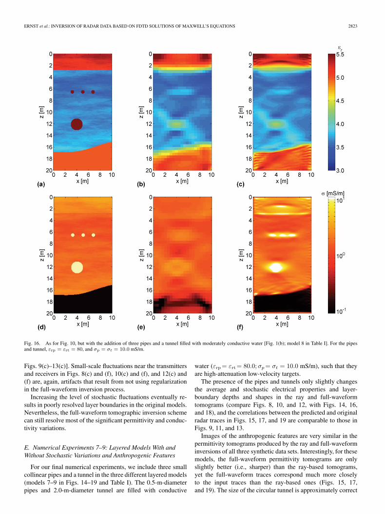
Fig. 16. As for Fig. 10, but with the addition of three pipes and a tunnel filled with moderately conductive water [Fig. 1(b); model 8 in Table I]. For the pipesand tunnel, εrp = εrt = 80, and σp = σt = 10.0 mS/m.
Figs. 9(c)–13(c)]. Small-scale fluctuations near the transmittersand receivers in Figs. 8(c) and (f), 10(c) and (f), and 12(c) and(f) are, again, artifacts that result from not using regularizationin the full-waveform inversion process.
Increasing the level of stochastic fluctuations eventually re-sults in poorly resolved layer boundaries in the original models.Nevertheless, the full-waveform tomographic inversion schemecan still resolve most of the significant permittivity and conduc-tivity variations.
E. Numerical Experiments 7–9: Layered Models With andWithout Stochastic Variations and Anthropogenic Features
For our final numerical experiments, we include three smallcollinear pipes and a tunnel in the three different layered models(models 7–9 in Figs. 14–19 and Table I). The 0.5-m-diameterpipes and 2.0-m-diameter tunnel are filled with conductive
water (εrp = εrt = 80.0;σp = σt = 10.0 mS/m), such that theyare high-attenuation low-velocity targets.
The presence of the pipes and tunnels only slightly changesthe average and stochastic electrical properties and layer-boundary depths and shapes in the ray and full-waveformtomograms (compare Figs. 8, 10, and 12, with Figs. 14, 16,and 18), and the correlations between the predicted and originalradar traces in Figs. 15, 17, and 19 are comparable to those inFigs. 9, 11, and 13.
Images of the anthropogenic features are very similar in thepermittivity tomograms produced by the ray and full-waveforminversions of all three synthetic data sets. Interestingly, for thesemodels, the full-waveform permittivity tomograms are onlyslightly better (i.e., sharper) than the ray-based tomograms,yet the full-waveform traces correspond much more closelyto the input traces than the ray-based ones (Figs. 15, 17,and 19). The size of the circular tunnel is approximately correct
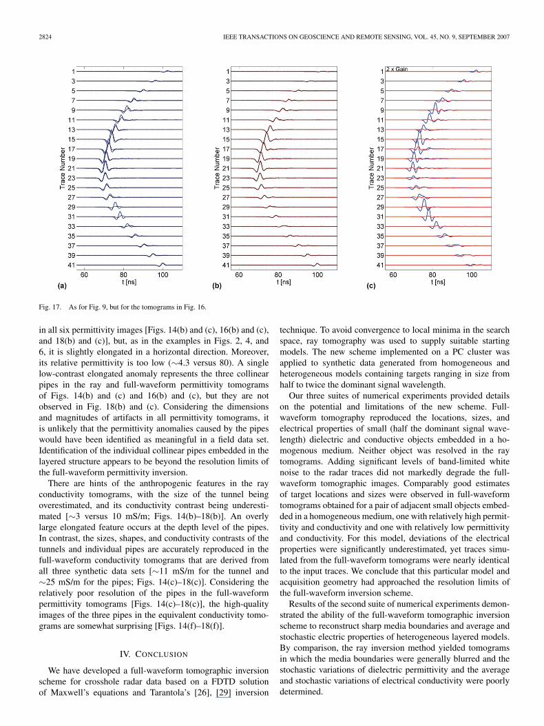
2824 IEEE TRANSACTIONS ON GEOSCIENCE AND REMOTE SENSING, VOL. 45, NO. 9, SEPTEMBER 2007
Fig. 17. As for Fig. 9, but for the tomograms in Fig. 16.
in all six permittivity images [Figs. 14(b) and (c), 16(b) and (c),and 18(b) and (c)], but, as in the examples in Figs. 2, 4, and6, it is slightly elongated in a horizontal direction. Moreover,its relative permittivity is too low (∼4.3 versus 80). A singlelow-contrast elongated anomaly represents the three collinearpipes in the ray and full-waveform permittivity tomogramsof Figs. 14(b) and (c) and 16(b) and (c), but they are notobserved in Fig. 18(b) and (c). Considering the dimensionsand magnitudes of artifacts in all permittivity tomograms, itis unlikely that the permittivity anomalies caused by the pipeswould have been identified as meaningful in a field data set.Identification of the individual collinear pipes embedded in thelayered structure appears to be beyond the resolution limits ofthe full-waveform permittivity inversion.
There are hints of the anthropogenic features in the rayconductivity tomograms, with the size of the tunnel beingoverestimated, and its conductivity contrast being underesti-mated [∼3 versus 10 mS/m; Figs. 14(b)–18(b)]. An overlylarge elongated feature occurs at the depth level of the pipes.In contrast, the sizes, shapes, and conductivity contrasts of thetunnels and individual pipes are accurately reproduced in thefull-waveform conductivity tomograms that are derived fromall three synthetic data sets [∼11 mS/m for the tunnel and∼25 mS/m for the pipes; Figs. 14(c)–18(c)]. Considering therelatively poor resolution of the pipes in the full-waveformpermittivity tomograms [Figs. 14(c)–18(c)], the high-qualityimages of the three pipes in the equivalent conductivity tomo-grams are somewhat surprising [Figs. 14(f)–18(f)].
IV. CONCLUSION
We have developed a full-waveform tomographic inversionscheme for crosshole radar data based on a FDTD solutionof Maxwell’s equations and Tarantola’s [26], [29] inversion
technique. To avoid convergence to local minima in the searchspace, ray tomography was used to supply suitable startingmodels. The new scheme implemented on a PC cluster wasapplied to synthetic data generated from homogeneous andheterogeneous models containing targets ranging in size fromhalf to twice the dominant signal wavelength.
Our three suites of numerical experiments provided detailson the potential and limitations of the new scheme. Full-waveform tomography reproduced the locations, sizes, andelectrical properties of small (half the dominant signal wave-length) dielectric and conductive objects embedded in a ho-mogenous medium. Neither object was resolved in the raytomograms. Adding significant levels of band-limited whitenoise to the radar traces did not markedly degrade the full-waveform tomographic images. Comparably good estimatesof target locations and sizes were observed in full-waveformtomograms obtained for a pair of adjacent small objects embed-ded in a homogeneous medium, one with relatively high permit-tivity and conductivity and one with relatively low permittivityand conductivity. For this model, deviations of the electricalproperties were significantly underestimated, yet traces simu-lated from the full-waveform tomograms were nearly identicalto the input traces. We conclude that this particular model andacquisition geometry had approached the resolution limits ofthe full-waveform inversion scheme.
Results of the second suite of numerical experiments demon-strated the ability of the full-waveform tomographic inversionscheme to reconstruct sharp media boundaries and average andstochastic electric properties of heterogeneous layered models.By comparison, the ray inversion method yielded tomogramsin which the media boundaries were generally blurred and thestochastic variations of dielectric permittivity and the averageand stochastic variations of electrical conductivity were poorlydetermined.
ERNST et al.: INVERSION OF RADAR DATA BASED ON FDTD SOLUTIONS OF MAXWELL’S EQUATIONS 2825
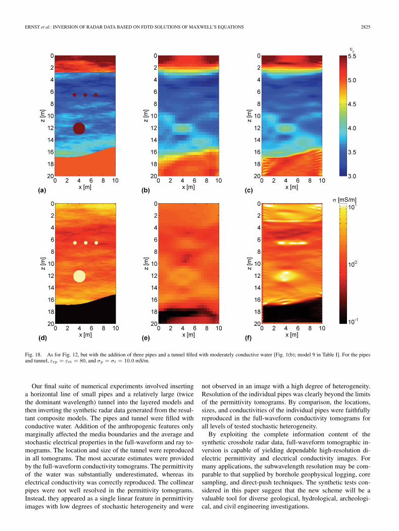
Fig. 18. As for Fig. 12, but with the addition of three pipes and a tunnel filled with moderately conductive water [Fig. 1(b); model 9 in Table I]. For the pipesand tunnel, εrp = εrt = 80, and σp = σt = 10.0 mS/m.
Our final suite of numerical experiments involved insertinga horizontal line of small pipes and a relatively large (twicethe dominant wavelength) tunnel into the layered models andthen inverting the synthetic radar data generated from the resul-tant composite models. The pipes and tunnel were filled withconductive water. Addition of the anthropogenic features onlymarginally affected the media boundaries and the average andstochastic electrical properties in the full-waveform and ray to-mograms. The location and size of the tunnel were reproducedin all tomograms. The most accurate estimates were providedby the full-waveform conductivity tomograms. The permittivityof the water was substantially underestimated, whereas itselectrical conductivity was correctly reproduced. The collinearpipes were not well resolved in the permittivity tomograms.Instead, they appeared as a single linear feature in permittivityimages with low degrees of stochastic heterogeneity and were
not observed in an image with a high degree of heterogeneity.Resolution of the individual pipes was clearly beyond the limitsof the permittivity tomograms. By comparison, the locations,sizes, and conductivities of the individual pipes were faithfullyreproduced in the full-waveform conductivity tomograms forall levels of tested stochastic heterogeneity.
By exploiting the complete information content of thesynthetic crosshole radar data, full-waveform tomographic in-version is capable of yielding dependable high-resolution di-electric permittivity and electrical conductivity images. Formany applications, the subwavelength resolution may be com-parable to that supplied by borehole geophysical logging, coresampling, and direct-push techniques. The synthetic tests con-sidered in this paper suggest that the new scheme will be avaluable tool for diverse geological, hydrological, archeologi-cal, and civil engineering investigations.

2826 IEEE TRANSACTIONS ON GEOSCIENCE AND REMOTE SENSING, VOL. 45, NO. 9, SEPTEMBER 2007
Fig. 19. As for Fig. 9, but for the tomograms in Fig. 18.
ACKNOWLEDGMENT
The authors would like to thank the Hreidar group, ETHZurich for allowing the authors to access its high-performancecluster. This is ETH-Geophysics Publication 1476.
REFERENCES
[1] S. Carlsten, S. Johansson, and A. Worman, “Radar techniques for indi-cating internal erosion in embankment dams,” J. Appl. Geophys., vol. 33,no. 1–3, pp. 143–156, Jan. 1995.
[2] P. K. Fullagar, D. W. Livelybrooks, P. Zhang, A. J. Calvert, and Y. R.Wu, “Radio tomography and borehole radar delineation of the McConnellnickel sulfide deposit, Sudbury, Ontario, Canada,” Geophysics, vol. 65,no. 6, pp. 1920–1930, Nov./Dec. 2000.
[3] G. Bellefleur and M. Chouteau, “Massive sulphide delineation using bore-hole radar: Tests at the McConnell nickel deposit, Sudbury, Ontario,”J. Appl. Geophys., vol. 47, no. 1, pp. 45–61, May 2001.
[4] K. Holliger, M. Musil, and H. R. Maurer, “Ray-based amplitude tomog-raphy for crosshole georadar data: A numerical assessment,” J. Appl.Geophys., vol. 47, no. 3/4, pp. 285–298, Jul. 2001.
[5] J. Tronicke, D. R. Tweeton, P. Dietrich, and E. Appel, “Improved cross-hole radar tomography by using direct and reflected arrival times,” J. Appl.Geophys., vol. 47, no. 2, pp. 97–105, Jun. 2001.
[6] K. Holliger and H. Maurer, “Effects of stochastic heterogeneity on ray-based tomographic inversion of crosshole georadar amplitude data,”J. Appl. Geophys., vol. 56, no. 3, pp. 177–193, Oct. 2004.
[7] J. D. Irving and R. J. Knight, “Effect of antennas on velocity estimatesobtained from crosshole GPR data,” Geophysics, vol. 70, no. 5, pp. K39–K42, Sep./Oct. 2005.
[8] W. P. Clement and W. Barrash, “Crosshole radar tomography in a fluvialaquifer near Boise, Idaho,” J. Environ. Eng. Geophys., vol. 11, no. 3,pp. 171–184, 2006.
[9] M. Musil, H. Maurer, K. Hollinger, and A. G. Green, “Internal structureof an alpine rock glacier based on crosshole georadar traveltimes andamplitudes,” Geophys. Prospect., vol. 54, no. 3, pp. 273–285, May 2006.
[10] H. Paasche, J. Tronicke, K. Holliger, A. G. Green, and H. Maurer, “In-tegration of diverse physical-property models: Subsurface zonation andpetrophysical parameter estimation based on fuzzy c-means cluster analy-ses,” Geophysics, vol. 71, no. 3, pp. H33–H44, 2006.
[11] G. Nolet, Seismic Wave Propagation and Seismic Tomography: SeismicTomography With Application in Global Seismology and ExplorationGeophysics, G. Nolet, Ed. Amsterdam, The Netherlands: Reidel, 1987.
[12] E. Wielandt, On the Validity of the Ray Approximation for Interpret-ing Delay Times: Seismic Tomography With Applications in GlobalSeismology and Exploration Geophysics, G. Nolet, Ed. Amsterdam,The Netherlands: Reidel, 1987.
[13] P. R. Williamson and M. H. Worthington, “Resolution limits in ray to-mography due to wave behavior—Numerical experiments,” Geophysics,vol. 58, no. 5, pp. 727–735, May 1993.
[14] V. Cerveny and J. E. P. Soares, “Fresnel volume ray tracing,” Geophysics,vol. 57, no. 7, pp. 902–915, Jul. 1992.
[15] J. Spetzler and R. Snieder, “The Fresnel volume and transmitted waves,”Geophysics, vol. 69, no. 3, pp. 653–663, May/Jun. 2004.
[16] Y. Luo and G. T. Schuster, “Wave-equation traveltime inversion,”Geophysics, vol. 56, no. 5, pp. 645–653, May 1991.
[17] D. W. Vasco and E. L. Majer, “Wavepath travel-time tomography,”Geophys. J. Int., vol. 115, no. 3, pp. 1055–1069, Dec. 1993.
[18] C. X. Zhou, W. Y. Cai, Y. Luo, G. T. Schuster, and S. Hassanzadeh,“Acoustic wave-equation travel-time and wave-form inversion of cross-hole seismic data,” Geophysics, vol. 60, no. 3, pp. 765–773, May/Jun. 1995.
[19] C. X. Zhou, G. T. Schuster, S. Hassanzadeh, and J. M. Harris, “Elasticwave equation traveltime and waveform inversion of crosswell data,”Geophysics, vol. 62, no. 3, pp. 853–868, May/Jun. 1997.
[20] A. J. Devaney, “Geophysical diffraction tomography,” IEEE Trans.Geosci. Remote Sens., vol. GRS-22, no. 1, pp. 3–13, Jan. 1984.
[21] R. S. Wu and M. N. Toksoz, “Diffraction tomography and multisourceholography applied to seismic imaging,” Geophysics, vol. 52, no. 1,pp. 11–25, Jan. 1987.
[22] R. G. Pratt and M. H. Worthington, “The application of diffractiontomography to cross-hole seismic data,” Geophysics, vol. 53, no. 10,pp. 1284–1294, Oct. 1988.
[23] M. J. Woodward, “Wave-equation tomography,” Geophysics, vol. 57,no. 1, pp. 15–26, Jan. 1992.
[24] T. A. Dickens, “Diffraction tomography for crosswell imaging of nearlylayered media,” Geophysics, vol. 59, no. 5, pp. 694–706, May 1994.
[25] J. M. Harris and G. Y. Wang, “Diffraction tomography for inhomo-geneities in layered background medium,” Geophysics, vol. 61, no. 2,pp. 570–583, Mar./Apr. 1996.
[26] A. Tarantola, “Inversion of seismic-reflection data in the acoustic approx-imation,” Geophysics, vol. 49, no. 8, pp. 1259–1266, Aug. 1984.
[27] A. Tarantola, “The seismic reflection inverse problem,” in Inverse Prob-lems of Acoustic and Elastic Waves, F. Santosa, Y.-H. Pao, W. Symes,and C. Holland, Eds. Philadelphia, PA: Soc. Ind. and Appl. Math.,1984.
[28] A. Tarantola, “A strategy for nonlinear elastic inversion of seismic-reflection data,” Geophysics, vol. 51, no. 10, pp. 1893–1903, Oct. 1986.

ERNST et al.: INVERSION OF RADAR DATA BASED ON FDTD SOLUTIONS OF MAXWELL’S EQUATIONS 2827
[29] A. Tarantola, Inverse Problem Theory and Methods for Model ParameterEstimation. Philadelphia, PA: Soc. Ind. and Appl. Math., 2005.
[30] O. Gauthier, J. Virieux, and A. Tarantola, “Two-dimensional nonlinearinversion of seismic wave-forms—Numerical results,” Geophysics,vol. 51, no. 7, pp. 1387–1403, Jul. 1986.
[31] P. Mora, “Nonlinear two-dimensional elastic inversion of multioffset seis-mic data,” Geophysics, vol. 52, no. 9, pp. 1211–1228, Sep. 1987.
[32] W. B. Beydoun, J. Delvaux, M. Mendes, G. Noual, and A. Tarantola,“Practical aspects of an elastic migration-inversion of crosshole data forreservoir characterization—A Paris basin example,” Geophysics, vol. 54,no. 12, pp. 1587–1595, Dec. 1989.
[33] A. Pica, J. P. Diet, and A. Tarantola, “Nonlinear inversion of seismic-reflection data in a laterally invariant medium,” Geophysics, vol. 55, no. 3,pp. 284–292, Mar. 1990.
[34] R. G. Pratt and M. H. Worthington, “Inverse-theory applied to multi-source cross-hole tomography. Part 1: Acoustic wave-equation method,”Geophys. Prospect., vol. 38, no. 3, pp. 287–310, Apr. 1990.
[35] R. G. Pratt, “Frequency-domain elastic wave modeling by finite-differences—A tool for crosshole seismic imaging,” Geophysics, vol. 55,no. 5, pp. 626–632, May 1990.
[36] R. G. Pratt, “Inverse-theory applied to multisource cross-hole tomogra-phy. Part 2: Elastic wave-equation method,” Geophys. Prospect., vol. 38,no. 3, pp. 311–329, Apr. 1990.
[37] R. G. Pratt, “Seismic waveform inversion in the frequency domain, Part 1:Theory and verification in a physical scale model,” Geophysics, vol. 64,no. 3, pp. 888–901, May/Jun. 1999.
[38] R. G. Pratt, Q. Li, B. C. Dyer, N. R. Goulty, and M. H. Worthington, “Al-gorithms for eor imaging using crosshole seismic data—An experimentwith scale-model data,” Geoexploration, vol. 28, no. 3/4, pp. 193–220,1991.
[39] R. G. Pratt and N. R. Goulty, “Combining wave-equation imaging withtraveltime tomography to form high-resolution images from crossholedata,” Geophysics, vol. 56, no. 2, pp. 208–224, Feb. 1991.
[40] Z. M. Song, P. R. Williamson, and R. G. Pratt, “Frequency-domainacoustic-wave modeling and inversion of crosshole data. Part 2. Inversionmethod, synthetic experiments and real-data results,” Geophysics, vol. 60,no. 3, pp. 796–809, May/Jun. 1995.
[41] D. T. Reiter and W. Rodi, “Nonlinear waveform tomography appliedto crosshole seismic data,” Geophysics, vol. 61, no. 3, pp. 902–913,May/Jun. 1996.
[42] R. G. Pratt and R. M. Shipp, “Seismic waveform inversion in the fre-quency domain, Part 2: Fault delineation in sediments using crossholedata,” Geophysics, vol. 64, no. 3, pp. 902–914, May/Jun. 1999.
[43] B. Zhou and S. A. Greenhalgh, “A damping method for 2.5-D Green’sfunction for arbitrary acoustic media,” Geophys. J. Int., vol. 144, pp. 111–120, 1998.
[44] B. Zhou and S. A. Greenhalgh, “Crosshole acoustic velocity imaging withthe full-waveform spectral data: 2.5-D numerical simulations,” Explor.Geophys., vol. 29, pp. 680–684, 1998.
[45] B. Zhou and S. A. Greenhalgh, “Crosshole seismic inversion withnormalized full-waveform amplitude data,” Geophysics, vol. 68, no. 4,pp. 1320–1330, Jul./Aug. 2003.
[46] G. J. Hicks and R. G. Pratt, “Reflection waveform inversion using localdescent methods: Estimating attenuation and velocity over a gas–sanddeposit,” Geophysics, vol. 66, no. 2, pp. 598–612, Mar./Apr. 2001.
[47] J. X. Dessa and G. Pascal, “Combined traveltime and frequency-domainseismic waveform inversion: A case study on multi-offset ultrasonic data,”Geophys. J. Int., vol. 154, no. 1, pp. 117–133, Jul. 2003.
[48] Y. M. Wang and W. C. Chew, “An iterative solution of the two-dimensional electromagnetic inverse scattering problem,” Int. J. ImagingSyst. Technol., vol. 1, no. 1, pp. 100–108, 1989.
[49] W. C. Chew and Y. M. Wang, “Reconstruction of 2-dimensional permit-tivity distribution using the distorted Born iterative method,” IEEE Trans.Med. Imag., vol. 9, no. 2, pp. 218–225, Jun. 1990.
[50] A. G. Sena and M. N. Toksoz, “Simultaneous reconstruction of permit-tivity and conductivity for crosshole geometries,” Geophysics, vol. 55,no. 10, pp. 1302–1311, Oct. 1990.
[51] M. Moghaddam, W. C. Chew, and M. Oristaglio, “Comparison of the Borniterative method and Tarantola’s method for an electromagnetic time-domain inverse problem,” Int. J. Imaging Syst. Technol., vol. 3, no. 4,pp. 318–333, 1991.
[52] M. Moghaddam and W. C. Chew, “Nonlinear 2-dimensional velocityprofile inversion using time domain data,” IEEE Trans. Geosci. RemoteSens., vol. 30, no. 1, pp. 147–156, Jan. 1992.
[53] M. Moghaddam and W. C. Chew, “Study of some practical issues ininversion with the Born iterative method using time-domain data,” IEEETrans. Antennas Propag., vol. 41, no. 2, pp. 177–184, Feb. 1993.
[54] T. J. Cui, W. C. Chew, A. A. Aydiner, and S. Y. Chen, “Inverse scatteringof two-dimensional dielectric objects buried in a lossy earth using the dis-torted Born iterative method,” IEEE Trans. Geosci. Remote Sens., vol. 39,no. 2, pp. 339–346, Feb. 2001.
[55] T. C. Johnson, P. S. Routh, and M. D. Knoll, “Fresnel volume georadarattenuation-difference tomography,” Geophys. J. Int., vol. 162, no. 1,pp. 9–24, Jul. 2005.
[56] W. Y. Cai, F. H. Qin, and G. T. Schuster, “Electromagnetic velocityinversion using 2-D Maxwell’s equations,” Geophysics, vol. 61, no. 4,pp. 1007–1021, Jul./Aug. 1996.
[57] C. G. Zhou and L. B. Liu, “Radar-diffraction tomography using themodified quasi-linear approximation,” IEEE Trans. Geosci. Remote Sens.,vol. 38, no. 1, pp. 404–415, Jan. 2000.
[58] H. Zhou, M. Sato, T. Takenaka, and G. Li, “Reconstruction from antenna-transformed radar data using a time-domain reconstruction method,”IEEE Trans. Geosci. Remote Sens., vol. 45, no. 3, pp. 689–696,Mar. 2007.
[59] T. J. Cui, Y. Qin, G. Y. Wang, and W. C. Chew, “Low-frequency detec-tion of two-dimensional buried objects using high-order extended Bornapproximations,” Inverse Probl., vol. 20, no. 6, pp. S41–S62, Dec. 2004.
[60] M. Strickel, A. Taflove, and K. Umashankar, “Finite-difference time-domain formulation of an inverse scattering scheme for remote-sensingof conducting and dielectric targets: Part 2: 2-dimensional case,” J. Elec-tromagn. Waves Appl., vol. 8, no. 4, pp. 509–529, 1994.
[61] M. Popovic and A. Taflove, “Two-dimensional FDTD inverse-scatteringscheme for determination of near-surface material properties at mi-crowave frequencies,” IEEE Trans. Antennas Propag., vol. 52, no. 9,pp. 2366–2373, Sep. 2004.
[62] T. J. Cui and W. C. Chew, “Novel diffraction tomographic algorithm forimaging two-dimensional targets buried under a lossy earth,” IEEE Trans.Geosci. Remote Sens., vol. 38, no. 4, pp. 2033–2041, Jul. 2000.
[63] T. J. Cui and W. C. Chew, “Diffraction tomographic algorithm for thedetection of three-dimensional objects buried in a lossy half-space,” IEEETrans. Antennas Propag., vol. 50, no. 1, pp. 42–49, Jan. 2002.
[64] J. R. Ernst, K. Holliger, H. Maurer, and A. G. Green, “Full-waveform in-version of crosshole georadar data,” presented at the SEG Int. Expositionand 75th Annu. Meeting, Houston, TX, 2005.
[65] H. T. Jia, T. Takenaka, and T. Tanaka, “Time-domain inverse scatteringmethod for cross-borehole radar imaging,” IEEE Trans. Geosci. RemoteSens., vol. 40, no. 7, pp. 1640–1647, Jul. 2002.
[66] S. Kuroda, M. Takeuchi, and H. J. Kim, “Full waveform inversion algo-rithm for interpreting cross-borehole GPR data,” in Proc. SEG Int. Expo.and 75th Annu. Meeting, Houston, TX, 2005, pp. 1176–1179.
[67] K. Holliger and T. Bergmann, “Numerical modeling of borehole georadardata,” Geophysics, vol. 67, no. 4, pp. 1249–1257, Jul./Aug. 2002.
[68] J. R. Ernst, K. Holliger, H. Maurer, and A. G. Green, “Realistic FDTDmodelling of borehole georadar antenna radiation: Methodology andapplication,” Near Surf. Geophys., vol. 4, pp. 19–30, 2006.
[69] T. Bergmann, J. O. A. Robertsson, and K. Holliger, “Numerical proper-ties of staggered finite-difference solutions of Maxwell’s equations forground-penetrating radar modeling,” Geophys. Res. Lett., vol. 23, no. 1,pp. 45–48, 1996.
[70] T. Bergmann, J. O. A. Robertsson, and K. Holliger, “Finite-differencemodeling of electromagnetic wave propagation in dispersive and atten-uating media,” Geophysics, vol. 63, no. 3, pp. 856–867, 1998.
[71] T. Bergmann, J. O. Blanch, J. O. A. Robertsson, and K. Holliger, “Asimplified Lax–Wendroff correction for staggered-grid FDTD modelingof electromagnetic wave propagation in frequency-dependent media,”Geophysics, vol. 64, no. 5, pp. 1369–1377, 1999.
[72] K. Holliger and T. Bergmann, “Accurate and efficient FDTD modeling ofground-penetrating radar antenna radiation,” Geophys. Res. Lett., vol. 25,no. 20, pp. 3883–3886, 1998.
[73] B. Lampe, K. Holliger, and A. G. Green, “A finite-differencetime-domain simulation tool for ground-penetrating radar antennas,”Geophysics, vol. 68, no. 3, pp. 971–987, May/Jun. 2003.
[74] B. Lampe and K. Holliger, “Effects of fractal fluctuations in topographicrelief, permittivity and conductivity on ground-penetrating radar antennaradiation,” Geophysics, vol. 68, no. 6, pp. 1934–1944, Nov./Dec. 2003.
[75] B. Lampe and K. Holliger, “Resistively loaded antennas for ground-penetrating radar: A modeling approach,” Geophysics, vol. 70, no. 3,pp. K23–K32, May/Jun. 2005.
[76] A. Taflove and S. C. Hagness, Computational Electrodynamics the Finite-Difference Time-Domain Method, 2nd ed. Boston, MA: Artech House,2000.
[77] K. S. Yee, “Numerical solution of initial boundary value problems in-volving Maxwell’s equations in isotropic media,” IEEE Trans. AntennasPropag., vol. AP-14, no. 3, pp. 302–307, May 1966.

2828 IEEE TRANSACTIONS ON GEOSCIENCE AND REMOTE SENSING, VOL. 45, NO. 9, SEPTEMBER 2007
[78] J. P. Berenger, “A perfectly matched layer for the absorption ofelectromagnetic-waves,” J. Comput. Phys., vol. 114, no. 2, pp. 185–200,Oct. 1994.
[79] J. Y. Fang and Z. H. Wu, “Generalized perfectly matched layer for theabsorption of propagating and evanescent waves in lossless and lossymedia,” IEEE Trans. Microw. Theory Tech., vol. 44, no. 12, pp. 2216–2222, Dec. 1996.
[80] J. D. Jackson, Classical Electrodynamics, 2nd ed. New York: Wiley,1975.
[81] E. Polak and G. Ribiere, “Note on convergence of conjugate directionmethods,” Revue Francaise d’Informatique de Recherche Operationnelle,vol. 3, pp. 35–43, 1969.
[82] T. Watanabe, K. T. Nihei, S. Nakagawa, and L. R. Myer, “Viscoacousticwaveform inversion of transmission data for velocity and attenuation,”J. Acoust. Soc. Amer., vol. 115, no. 6, pp. 3059–3067, Jun. 2004.
[83] T. A. Hewett, “Fractal distribution of reservoir heterogeneity and theirinfluence on fluid transport,” presented at the 61st Annu. Technical Conf.SPE, New Orleans, LA, 1986, Paper SPE 15386.
[84] J. A. Goff and J. W. Jennings, “Improvement of Fourier-based uncondi-tional and conditional simulations for band limited fractal (von Karman)statistical models,” Math. Geol., vol. 31, no. 6, pp. 627–649, Aug. 1999.
[85] J. Tronicke and K. Holliger, “Quantitative integration of hydrogeophys-ical data: Conditional geostatistical simulation for characterizing het-erogeneous alluvial aquifers,” Geophysics, vol. 70, no. 3, pp. H1–H10,May/Jun. 2005.
Jacques R. Ernst (S’07) received the M.S. de-gree in applied and environmental geophysics fromthe Swiss Federal Institute of Technology (ETH),Zurich, Switzerland, in 2002, where he is currentlyworking toward the Ph.D. degree in geophysics.
His current research interests include simulationof realistic ground penetrating radar (GPR) antennasand full-waveform modeling and inversion of cross-borehole GPR data.
Mr. Ernst is a member of Society of ExplorationGeophysicists (SEG).
Hansruedi Maurer received the M.S. and Ph.D. de-grees in geophysics from the Swiss Federal Instituteof Technology (ETH), Zurich, Switzerland.
He was with the Geological Survey of Canada,Ottawa, ON, Canada, for six months. In 1993, hejoined the Applied and Environmental GeophysicsGroup, Institute of Geophysics, ETH, where he iscurrently a Senior Research Scientist. Since 2000,he has been an Associate Editor of Geophysics.His main research interests are the inversion theoryand its applications to diverse geophysical datasets,
including crosshole georadar data.Dr. Maurer received the Best Poster Award from the Society of Exploration
Geophysics in 1998 for his contributions to statistical experimental designs.
Alan G. Green completed his studies at Britishuniversities before moving to Canada in 1973.
After a one-year Postdoctoral Fellowship at theEarth Physics Branch, Ottawa, ON, Canada, he be-came an Assistant Professor of geophysics at theUniversity of Manitoba, Winnipeg, MB, Canada. In1979, he accepted an invitation to become the Headof the Lithospheric Geophysics Section, GeologicalSurvey of Canada, Ottawa. During his 19 years inCanada, he further developed and applied seismic re-flection methods in investigations of the continental
crust, studies associated with nuclear waste disposal, and mineral explorationin crystalline terranes. Shortly after a one-year sabbatical leave in Switzerland,he accepted an invitation to become a Professor of applied and environmentalgeophysics at the Institute of Geophysics, Swiss Federal Institute of Technology(ETH), Zurich, Switzerland.
Klaus Holliger received the M.Sc. and Ph.D. de-grees in geophysics from the Swiss Federal Instituteof Technology (ETH), Zurich, Switzerland, and apostgraduate degree in economics from the Univer-sity of London, London, U.K.
He was a Postdoc at Rice University, Houston, TX,and worked for extended periods at the U.S. Geologi-cal Survey, Menlo Park, CA; Imperial College, U.K.;and Cambridge University, U.K. He was a Lecturerwith the Applied and Environmental GeophysicsGroup, ETH, in 1994, became a Senior Lecturer in
1996, and became a Professor in 2002. In September 2005, he was the Chair inapplied and environmental geophysics at the University of Lausanne, Lausanne,Switzerland, and he currently serves as Vice-Dean of research. He also teachesat Ecole Polytechnique Fédérale de Lausanne and the University of Neuchatel.His main research interests include hydrogeophysics, geostatistical data fusion,and seismic and electromagnetic wave propagation phenomena in the shallowsubsurface.