JOURNAL OF GEOPHYSICAL RESEARCH, VOL. 98, NO. B2, PAGES 1777-1792, FEBRUARY 10, 1993

Shallow Structure of Oceanic Crust in the Western North Atlantic From Seismic Waveform Inversion and Modeling

TIMOTHY A. MINSHULL

Bullard Laboratories, Department of Earth Sciences, University of Cambridge, England

SATISH C. SINGH

British Institutions Reflection Profiling Syndicate and Institute of Theoretical Geophysics, Bullard Laboratories, Cambridge, England

Seismic reflection data from Mesozoic oceanic crust in the western North Atlantic, in the vicinity of the Blake Spur Fracture Zone, have imaged a number of short, subhorizontal events in the upper 1 km of the crystalline crust. Wide-angle expanding spread profile (ESP) data from the same region indicate the presence of first-order velocity discontinuities in this depth interval. Using ESP data reprocessed to enhance precritical reflection events, we investigate the relationship between the precritical and postcritical reflections with three different approaches: amplitude analysis, forward modeling, and waveform inversion. The precritical reflections have high apparent reflection coet•cients (~ 0.1) and may be divided into two types: those which can be traced out to critical ranges (5-6 km), representing velocity steps, and those which fade out at ranges of 3-4 kin, representing shorter-wavelength velocity variations. Synthetic seismogram modeling indicates that the velocity steps occur within a 50 m depth interval, while the shorter-wavelength features may correspond to high- or low-velocity zones with a thickness of 20 m (10% of the dominant seismic wavelength) or less. We investigate the velocity structure in detail by full waveform inversion of a selected portion of ESP data, transformed into the intercept time-slowness domain. The inversion method minimizes the sample-by-sample misfit between the data and reflectivity synthetics in a least squares sense. A conjugate gradient algorithm was used, starting from a velocity structure derived from forward modeling of wide-angle ESP data. The inversion tightly constrains short-wavelength components of the velocity structure, and indicates that intracrustal reflections result both from major velocity steps and from zones of alternating high and low velocity. Synthetic seismograms generated from sonic log data from Deep Sea Drilling Project hole 418A show reflections of similar amplitude and character to those seen in the ESP data. These reflections probably originate from rather subtle features of the velocity-depth profile, related primarily to changes in porosity in the pillow lava sequence. A deeper reflector, 800 ms below oceanic basement in the Blake Spur Fracture Zone, may correspond to the top of a zone of serpentinized upper mantle.

INTRODUCTION

For young oceanic crust at fast spreading ridges, the detailed structure of the upper part of layer 2 may be readily investigated using first-arrival energy from sur- face [e.g. Harding e! al., 1989; Vera et al., 1990] and ocean bottom [e.g. Purdy, 1987] seismic sources and receivers. However, on old, sedimented oceanic crust, postcritical energy from this part of the crust is ob- scured by reflections from the water bottom and sedi- ments, and precritical reflections are contaminated by multiples. A smoothed velocity structure for the up- permost crust may be derived using borehole seismic methods [e.g. Swift et al., 1988], but such studies are necessarily limited to a very few localities. Several stud- ies using surface seismic data have concentrated on the sediment-basement transition [White, 1979; White and Stephen, 1980; Rohr, 1987], and these studies indicate that this transition varies from a sharp discontinuity

Copyright 1993 by the American Geophysical Union.

Papor numbor 92JB02136. 0148-0227/93/92JB-02136505.00

to a gradient zone up to 300 m thick. Many exper- iments have constrained the long-wavelength velocity- depth variation in the upper crust, but data quality is rarely good enough to look in detail beneath this tran- sition.

A large data set of ESPs and reflection profiles was acquired on Mesozoic oceanic crust in the western North Atlantic in November-December 1987 (Figure 1). Nineteen ESPs were acquired: 15 flowline profiles at the Blake Spur Fracture Zone and across a ribbon of "nor- mal" oceanic crust extending to an unnamed fracture zone to the north, and four isochron profiles. Simulta- neous reflection profiles were acquired along the tracks of the ESPs, and further single-ship reflection profiles completed the survey. Details of the experiment, pro- cessing and synthetic seismogram modeling of post criti- cal arrivals from eight profiles in the immediate vicinity of the Blake Spur Fracture Zone (ESPs 1-8) are given by Minshull e! al. [1991]. The reflection profiles im- aged many intracrustal reflectors [While ½! al., 1990; E. Morris et al., Seismic structure of oceanic crust in the western North Atlantic, submitted to J. Geophys. Res., 1992], including a number of short (up to 3 km long)

1777

1778 IV[INSHULL AND SINGH: UPPER OCEANIC CRUST

29øN

28øN

27øN

26øN

72 ø W 70 ø W

I

•,...' Hatteras Abyssal Plain

ß

BERMUDA

,

!

¾.... ß 418

50 km I I

68 ø W

Fig. 1. Location of two-ship seismic experiment. Solid lines mark R/V Conrad tracks, and thicker lines mark expanding spread profiles (ESPs) in the vicinity of the Blake Spur Fracture Zone [Minshull et al., 1991], and published reflection profiles 699 and 711 [White et al., 1990]. Filled circle marks Deep Sea Drilling Project (DSDP) Site 418.

subhorizontal reflectors in the uppermost few hundred meters of the crust. Although energy from this part of the crust is often scattered and incoherent, and may be obscured in the reflection data by diffractions due to the rough topography at the top of oceanic layer 2, later- ally coherent reflectors appear clearly at some locations (Figure 2).

Triplications in the ESP data also indicated the presence of velocity discontinuities within oceanic layer 2. However, the relationship between these discon- tinuities and the reflectors imaged on normal incidence data was not clear. A synthetic generated from an ideal- ized velocity structure consisting of gradient transitions and thin low-velocity zones (Figure 3) indicates that the reflections and the triplications need not be related at all, since gradient transitions reflect energy only at large angles of incidence, while thin low-velocity zones reflect only at near-normal incidence. Here we investigate the origin of upper crustal reflections in detail by quantita• tive amplitude studies, synthetic seismogram modeling and waveform inversion of precritical intracrustal reflec- tions detected in the ESP data. We also illustrate the

long-recognized importance of the starting model in the

inversion procedure, and identify various sources of mis- fit between the inverted data and a synthetic generated from the final inversion model. The use of ESP data

limits us to a one-dimensional approach to a structure which is clearly three-dimensional; this approach is jus- tified because of the relative lateral homogeneity of the sediments, oceanic basement, and upper crust in the data set we use, the small offset range chosen, and the common-midpoint geometry.

AMPLITUDE ANALYSIS

This study focuses on ESP5, shot along the Blake Spur Fracture Zone, because this ESP had the highest data quality and conformed most closely to the one- dimensional assumption inherent in our methods. To confirm that the velocity structure of ESP5 is indeed typical of the uppermost oceanic crust in our survey area, we first compare velocities, reflection amplitudes and apparent reflection coefficients for this ESP with those obtained for a number of other ESPs.

In order to meaningfully measure and model ampli- tudes, partial reprocessing of the ESP data was neces- sary. The standard ESP processing sequence, including

MJNSHULL AND $INGH: UPPER OCEANIC CRUST 1779

w

7.o

ESP Midpoints lkm

9.0

1500 1400 1300

CDP

Fig. 2. Part of along-track reflection profile for ESP2. Arrows mark laterally coherent reflection events in the uppermost igneous crust. The filled bar marks the along-track spread of ESP midpoints at the time of minimum source-receiver range. Midpoints are offset ~ 400 m perpendicular to the profile.

1200

a constant offset stack across the streamer, enhances low-frequency wide-angle arrivals, but causes severe de- structive interference of precritical reflections in the presence of basement topography or reflector dip. For the 2.4 km streamer used in the Blake Spur experiment and a 4 km/s velocity at the top of oceanic layer 2, a re- flector dip of only 2.4 ø gives total cancellation of 20 Hz energy in a constant offset stack. Reflector dips were investigated by processing the ESP data into a 1.2 km common midpoint stack, using data out to 5 km range; the limit here is determined by the severe normal move- out stretch which results as reflectors merge and cross, rather than errors in the hyperbolic moveout approxi- mation, which are still less than 10 ms for intracrustal reflectors at this range. These short profiles image the true structure beneath the ESP midpoint, in contrast to the simultaneous reflection profile, which necessarily has its midpoint track offset by at least a few hundred meters (Figure 4). The structure imaged at ESP mid- points was quite complex, as might be expected from the associated reflection profiles (e.g. Figure 2). How- ever, in the case of four ESPs, intracrustal reflectors were imaged with enough horizontal coherence to allow

common offset stacking over part of the dataset without destructive interference.

Interval velocities were determined in detail for in-

tracrustal reflectors and for the overlying sediment col- umn by one-dimensional travel time modeling. In some locations, high velocity (2.5-3.0 km/s) sediments were detected immediately above the basement. A compi- lation of interval velocities in the crystalline crust is shown in Figure 5. Velocities in the top 800 m of oceanic crust fall in the range 3.7-4.7 km/s for all ESPs ana- lyzed in this way. Since intervals between reflectors are small, uncertainties in these velocities are large, up to 10% in some cases.

Reflection coefficients were calculated for in-

tracrustal reflectors by comparison with the seabed re- flection and its multiple, assuming a sea surface reflec- tion coefficient of-1 [e.g., Ansley, 1977]. The seabed reflection coefficient is also required to scale the for- ward modeling and inversion results which follow. Data from one high-quality ESP gave a seabed reflection co- efficient of 0.20 :t: 0.02, and other ESPs and reflection profiles in the survey area gave similar values. A value of 0.2 was used in all subsequent calculations. Travel-

1780 MINS•LL AND SINGH: UPPER OCEANIC CRUST

i

lO

.4

5

i i I I I I 1

2 4 6 8 10 12 14

Range (krn)

Fig. 3. Reflectivity synthetic for idealized crustal velocity model, reduced at 8 km/s, with p and s wave velocities shown in the inset. Densities were derived from p wave velocities as described in the text, and the source wavelet is shown in Figure 15. The sediment thickness and water depth are typical for the experiment area. Normal incidence reflections are generated by the basement (b) and by the three thin (5 m) intracrustal low-velocity zones (1-3). Wide-angle reflections are generated by the basement and the two gradient transition zones (4, 5).

time modeling of sediment reflectors indicated little ve- locity contrast across the seabed, as is commonly ob- served for abyssal sediments [e.g. $hipley, 1983]; the large impedance contrast here is mainly due to a den- sity contrast.

Normal incidence reflection coefficients were calcu-

lated for all intracrustal reflectors with large enough amplitude to be readily distinguished from the back- ground noise, using traces within 2.5 km range, except for ESP5, where ranges of 2.15-3 km were used. At normal incidence, the appropriate geometric spreading correction is proportional to two-way time multiplied

RECEIVING SHIP

SHOO'riNG SHIP

Tr•ck of Mmult•neous

rdfl©ctlon profile

Fig. 4. Schematic diagram showing the offset as the two ships cross between ESP midpoints and midpoints for a simultaneous reflection profile (thick lines).

by the square of root-mean-square velocity [Newman, 1973]. Hence reflection coefficients r were estimated as follows'

r- o.2 Actcv• ( 2 ) AwtwV2 w exp •rf y•.(ti/Qi) (1) i=1

where A½ and Aw are the amplitudes of the crustal re- flector and the seabed, respectively, tc and tw are their respective two-way times, vc and vw are their respec- tive root-mean-square velocities, f is the dominant fre- quency of around 20 Hz, t• is the two-way time through the overlying sediment layer (between 0.8 and 1.2 s), Q• is the sediment attenuation parameter, and t2 and Q• are the equivalent values for the igneous crust. Q values of 200 in the sediment and 400 in the crust were used; these values were estimated from detailed forward mod-

elling of ESP5 (see below). The resulting reflection coefficients, computed for

each trace, are illustrated as histograms in Figure 6, together with representative incoherent noise ampli- tudes from the same traces scaled in the same way. Scatter in amplitudes represents the effects of multiples and diffractions as well as real variations in impedance contrast. Reflection coefficients are generally in the re- gion of 0.1 (means marked by arrows), while noise levels

MINSHULL AND SING}I: UPPER OCEANIC CRUST 1781

0.2

•

O.8

Velocity !km/sl 4.0 4.5 5.0

i •

,, ,• ,,• • / •-

3.5 5•5 61:) 6.5

ODP HOLE 418A SONIC LOG

\• ODP HOLE 418A OSE

Fig. 5. P wave velocity compilation for uppermost Mesozoic oceanic crust. Triangles mark interval velocities from travel-time modeling of ESP precritical reflections in ~ 140 Ma crust, with filled triangles for ESP5, and bars mark estimated uncertainties. The smooth line marks velocities derived from the oblique seismic experiment at DSDP Hole 418A [Swift et aL, 1988]; the layered model marks velocities from sonic logs at Hole 418A [Moos, 1988; Broglia and Moos, 1988], averaged over 6-m intervals.

correspond to reflection coefficients of around 0.03-0.05, and the noise probably obscures many weaker reflec- tions. The reflectors identified in ESP5 have coefficients

typical of the observed range.

SYNTHETIC SEISMOGRAM MODELING

The rapid downward increase of velocity between the water column and the oceanic basement means that

the angle of incidence of seismic waves on intracrustal reflectors can be quite large (i.e., near to critical) for rel- atively small source-receiver distances (much less than the reflector depths). Even in noisy ESPs (Figure 7), a distinction can be made between those reflectors which

may be traced out toward the critical angle and those which are visible only at short offsets. For ESP5, which has a large signal-to-noise ratio after reprocessing, we performed detailed forward modeling and waveform in- version to tightly constrain the velocity variations giv- ing rise to the reflections.

Synthetic seismogram modeling required a detailed impedance structure for the overlying sediment. The velocity model previously obtained from travel times (Figure 8c, dashed line) was generally adequate, but the high amplitude of one sediment reflector (higher

than the seabed; marked "A" in Figure 8), which oc- curs throughout the experiment area at 0.5 s below the seabed, could only be matched by introducing a thin high-velocity layer. This reflector is identified elsewhere in the western North Atlantic as "Horizon A" [e.g. Tu- cholke, 1979; Shipley, 1983]. A sediment Poisson's ratio of 0.4 was assumed, and densities were calculated using the velocity-density relations of Hamilton [1978], except at the seabed where the density was chosen to match the computed reflection coefficient. An important factor in the generation of synthetics is the Q value assigned to the sediments. Field and laboratory measurements of Q in marine sediments often give values much less than 100 [e.g. Hamilton, 1972]. A value of 50 gives quite se- vere attenuation of a 20 Hz signal passing through i s of sediment. However, measurement of spectral amplitude ratios between top and bottom halves of the sediment column suggested no systematic loss of high frequen- cies. A Q value of 200 was estimated by reflectivity modelling [Fuchs and Miiller, 1971] of the amplitudes of peg-leg multiples from within the sediment column (figure 9).

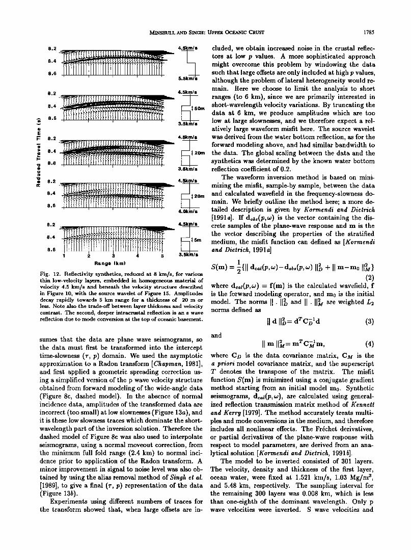
In the crystalline crust, a Poisson's ratio of 0.27 and the velocity-density relation of Christensen and Shaw [1970] were used. Reflectors with significant energy at both near and far offsets were modeled as major layer boundaries. For these reflectors to appear near normal incidence, the corresponding velocity transitions must take place over a depth interval less than around 50 m (Figure 10). Conversely, a reflector which appears near normal incidence but dies out at large offsets is most simply modeled as an isolated thin layer, with a large velocity contrast. Note that the thin layer tuning ef- fects are not necessary for a high amplitude reflection [Widess, 1973]; all that is required is a sufficiently large impedance contrast between the layer and the surround- ing medium. For a broad-band, near-minimum phase source wavelet as used in this experiment, the ampli- tudes of normal incidence reflections from such a layer are comparable with those from a velocity step with the same velocity contrast even for layer thicknesses of one-tenth of a wavelength (Figure 11). Synthetic seis- mogram studies of such layers have been carried out in a number of geological contexts [e.g. Fuchs, 1969; Hughes and Kennett, 1983], but not for oceanic crust. There is some degree of trade-off in modeling between layer thickness and velocity contrast (Figure 12), and the sign of the contrast is not well constrained by the amplitude variation, but a thickness of 5-20 m with a velocity contrast of 0.5-1.0 km/s is required to give high amplitude upper crustal reflections at normal incidence with amplitudes decreasing rapidly within a few kilo- meters offset. Multiples and mode conversions make important contributions to the reflection response, par- ticularly at large angles of incidence.

Hence modeling offset-dependent amplitude varia- tions allows us to distinguish three types of reflectors in the upper oceanic crust: (1) reflectors with both long-

1782 MINSHULL AND SINGH: UPPER OCEANIC CRUST

I

/

• I i I I I

'• • o

I

• •l I I I I I 0 o

0 • • a:) •0 •' Ol 0 -c•

o

o

o c•

o

o

•. I o u•

o

c• o o

o

o o. o

I

• I I I I I I l• m o

o

• o

o llll

o

ø 0

o

I

• •l I I I I I Ill o

seoeJ• 1o JeqtunN

MINSHULL AND SINGH: UPPER OCEANIC CRUST 1783

ESP1

2.0 3.0 4.0 5.0 6.0

ESP7

7.8

8.0

8.2

8.0

2.0 3.0 4.0 5.0 6.0

Range(kin) Fig. 7. Reprocessed precritical ESP data showing the basement reflector (b) and intracrustal reflectors (1-3), reduced at 8 km/s.

500m ESP5 I

(a) (b) ? ?

(o) (d) o

• t3

• 4

2 4 6

-i

Velocity (km\s)

10 I I I I I I

4 6 8 10 12

Range (km)

Fig. 8. (a) Near-offset ESP5 data reprocessed as CDP stack. Solid bar marks traces used in the common offset stack, and dashed lines mark reflections from the top of igneous basement (b), and three intracrustal reflectors (1-3). "A" marks high amplitude sedimentary reflector. No simultaneous reflection profile is available at the midpoint of this ESP. (b) Common offset stack of selected ESP5 traces, reduced at 8 km/s. (c) Solid line marks final p wave velocity-depth model for ESP5; dashed line marks original model from analysis of post-critical data. Q ',,,-dues are 200 in the sediment and 400 in the crust, and the reflector 1.4 km below the seabed is modeled as a thin (5 m) low-velocity zone. (d) Corresponding reflectivity synthetic, reduced at 8 km/s.

1784 1VIINSHULL AND SINGH: UPPER OCEANIC CRUST

lO

A 11

7 8 9 10 11 12

[[[Ir

ponents only, such as transition zones with steep ve- locity gradients, which give low amplitudes at normal incidence but a sharp increase at ranges where rays are focused by the gradient zone, and (3) reflectors with short-wavelength components only, such as sin- gle (or multiple) thin layers embedded in a surround- ing medium of constant velocity, which give offset- dependent tuning effects, and little or no post critical energy.

Based on the above analysis, a final synthetic for

Range (kin)

Fig. 9. Part of ESP5 data with reflectivity synthetics for estima- tion of sediment Q value. Travel times are unreduced, plots are scaled to the same water bottom reflection amplitude at normal incidence, and only the sediment Q value is varied between the synthetics. A trade-off exists between impedance contrast and Q value in forward modeling, and the synthetics do not include the effect of receiver directivity. For impedance contrasts based on interval velocity contrasts, a value of around 200 appears to give the best match to amplitude patterns in primaries and peg-leg multiples.

ESP5, with the corresponding velocity model, is shown in Figure 8d. Four reflectors were modeled in detail: the basement reflector, which here appears as an unusually sharp and laterally coherent boundary, and three in- tracrustal reflectors, two of type 1 and one of type 3. The type 3 reflector is modeled as a 5 m layer of anoma-

.• 1ously low velocity, but could equally well be a thicker layer (up to ~ 20 m) with a smaller velocity contrast,

? s 9 10 11 12 or have anomalously high velocity. The type I reflec- tors match closely in depth (within 300 m) two veloc- ity boundaries determined by triplications in the wide- angle data (dashed model). The difference in depth may represent minor lateral heterogeneity, but is barely sig- nificant, since at wide angle a 300-m transition zone is indistinguishable from a first-order discontinuity (Fig- ure 3).

WAVEFORM INVERSION

and short-wavelength velocity-depth components, such as first-order discontinuities, which show little change in amplitude with angle of incidence until close to the critical angle, (2) reflectors with long-wavelength com-

The data from ESP5 were also well suited to wave-

form inversion; this was used both as a check on the forward modeling result, and to elucidate further tails of the velocity structure. The method we use as-

160ms •-

100 50 20 0

Transition Thickness (m)

4.5kmls i

r

nsition

Depth 5.5kmls

Fig. 10. Near-normal incidence (100 m range) reflectivity synthetics for intracrustal gradient transition zones of various thicknesses and the source wavelet of Figure 15. The transition zone lies beneath 5.5 km of water, I km of sediment (velocity 2 km/s), and 0.5 km of basement (velocity 4.5 km/s). Note the decay in amplitude when the transition zone is more than 50 m thick.

150ms

100 40 20 10 4 2

Layer Thickness(m)

4km

I Layer

Depth

Fig. 11. Normal incidence synthetics generated by convolving the source wavelet of Figure 15 with two equal and opposite impedance contrasts separated by the thickness given. The reflection amplitude is comparable to the half-space response (infinite thickness) at thicknesses as low as 10-20 m (5-10% of a wavelength).

M. INSHIJLL AND SINGH: UPPER OCEANIC CRUST 1785

8.2

8.4

8.6

4.5 m/s

5.

8.2

8.4

8.6

8.2

8.4

8.6

8.2

8.4

8.6

4.5km/s

$ 50m

,,

3'.5km/s

4.5km/s

• t20m

3.5km/$

4.5. k•/. t 20m

8.2

8.4

8.6

Range (km)

:•.5km/s

Fig. 12. Reflectivity synthetics, reduced at 8 km/s, for various thin low-velocity layers, embedded in homogeneous material of velocity 4.5 km/s and beneath the velocity structure described in Figure 10, with the source wavelet of Figure 15. Amplitudes decay rapidly towards 5 km range for a thickness of 20 m or less. Note also the trade-off between layer thickness and velocity contrast. The second, deeper intracrustal reflection is an s wave reflection due to mode conversion at the top of oceanic basement.

sumes that the data are plane wave seismograms, so the data must first be transformed into the intercept time-slowness (r, p) domain. We used the asymptotic approximation to a Radon transform [Chapman, 1981], and first applied a geometric spreading correction us- ing a simplified version of the p wave velocity structure obtained from forward modeling of the wide-angle data (Figure 8c, dashed model). In the absence of normal incidence data, amplitudes of the transformed data are incorrect (too small)at low slownesses (Figure 13a), and it is these low slowness traces which dominate the short-

wavelength part of the inversion solution. Therefore the dashed model of Figure 8c was also used to interpolate seismograms, using a normal moveout correction, from the minimum full fold range (2.4 km) to normal inci- dence prior to application of the Radon transform. A minor improvement in signal to noise level was also ob- tained by using the alias removal method of $ingh et al. [1989], to give a final (r, p) representation of the data (Figure 13b).

Experiments using different numbers of traces for the transform showed that, when large offsets are in-

eluded, we obtain increased noise in the crustal reflec- tors at low p values. A more sophisticated approach might overcome this problem by windowing the data such that large offsets are only included at high p values, although the problem of lateral heterogeneity would re- main. Here we choose to limit the analysis to short ranges (to 6 km), since we are primarily interested in short-wavelength velocity variations. By truncating the data at 6 krn, we produce amplitudes which are too low at large slownesses, and we therefore expect a rel- atively large waveform misfit here. The source wavelet was derived from the water bottom reflection, as for the forward modeling above, and had similar bandwidth to the data. The global scaling between the data and the synthetics was determined by the known water bottom reflection coefficient of 0.2.

The waveform inversion method is based on mini-

mizing the misfit, sample-by sample, between the data and calculated wavefield in the frequency-slowness do- main. We briefly outline the method here; a more de- tailed description is given by Kormendi and Dietrich [1991a]. If dob,(p,w) is the vector containing the dis- crete samples of the plane-wave response and m is the the vector describing the properties of the stratified medium, the misfit function can defined as [tformendi and Dietrich, 1991a]

1

$(m)- {11 dca,(p,w)-dob•(p,w)I1• + II m-m0 I[•} where d,•,(p,•) - f(m) is the calculated wavefield, f is the forward modeling operator, and m0 is the initial model. The norms II. and II. I1, are weighted L2 norms defined as

and

II d I1>- d'CB ld (3)

II m IlY- mTc] TM, (4) where CD is the data covariance matrix, CM is the a priori model covariance matrix, and the superscript T denotes the transpose of the matrix. The misfit function $(m) is minimized using a conjugate gradient method starting from an initial model mo. Synthetic seismograms, dca•(p,w), are calculated using general- ized reflection transmission matrix method of Kennet!

and Kerry [1979]. The method accurately treats multi- ples and mode conversions in the medium, and therefore includes all nonlinear effects. The Frdchet derivatives, or partial derivatives of the plane-wave response with respect to model parameters, are derived from an ana- lytical solution [Kormendi and Dietrich, 1991b].

The model to be inverted consisted of 301 layers. The velocity, density and thickness of the first layer, ocean water, were fixed at 1.521 km/s, 1.03 Mg/m 3, and 5.48 km, respectively. The sampling interval for the remaining 300 layers was 0.008 km, which is less than one-eighth of the dominant wavelength. Only p wave velocities were inverted. S wave velocities and

1786 MINS• AND SINGH: UPPER OCEANIC CRUST

6.0

6.5

7.0

7.5

8.0

8.5

9.0

9.5

½<

> <

0.05 0.10 0.15 0.20 0.25 0.30 0.05 0.10 0.15 0.20 0.25 0.30

Slowness (s/km) Slowness (s/km)

Fig. 13. (a) Radon transform of reprocessed ESP5 data. Note the low amplitudes and linear artifacts at low slownesses due to the absence of near-normal incidence data. (b) Radon transform of ESP5 data after interpolation using the dashed velocity model of Figure 8a and alias removal using the same velocity model. Note the improved coherence and increased amplitude of reflectors at low slowness.

densities were fixed at starting values, derived from the initial p wave velocity model using the velocity-density relations and Poisson's ratios described in the previous section, throughout the inversion. Both have small ef- fects on the synthetic seismograms and hence on the inversion. Q values are fixed at 200 throughout. The data and model covariance matrices used were 0.025I

and I, respectively, where I is the identity matrix. The waveform inversion was performed in 6 different

runs with 5 iterations in each run. The starting model for each run was the final result of the previous run. The bandwidth of the data was increased progressively. The progressive inversion strategy (i.e., 6 runs) was used to decouple inversion of short and medium wavelengths of the velocity-depth model. This strategy is justified be- cause the short wavelengths of velocity are controlled by the waveform and the medium wavelengths by am- plitude variations along elliptical trajectories of the re- flectors in the (r, p) domain [Jannane e! al., 19881.

In the first run, the first five traces of Figure 12b were used. The data and the source wavelet were fil-

tered using a 6-26 Hz bandpass filter. The starting

model, derived by smoothing the model used for geo- metric spreading corrections and interpolation, is shown in Figure 14a and the corresponding synthetic seismo- gram for p = 0.05 s/km is shown in Figure 15a. The synthetic seismogram after five iterations is shown in Figure 15b. The cross-correlation coefficient for the syn- thetic and the real data (Figure 15f) for p = 0.05 s/km is 0.70.

In the next run, the number of traces was the same, but a preconditioning operator [Kormendi and Dietrich, 1991a] was applied to enhance the effect of later ar- rivals on the inversion. Furthermore, the bandwidth of the bandpass filter was changed to 3-40 Hz. The synthetic seismogram for p = 0.05 s/km, which has a cross-correlation coefficient of 0.72, is shown in Figure 15c. The short-wavelength velocity variation for the up- per part of the model was retrieved in these first two runs. In the third run, we used the first ten traces, to give the synthetic seismogram shown in Figure 15d. At this stage, the cross-correlations of the synthetic with the data were 0.74 for p = 0.05 s/km and 0.82 for p- 0.10 s/km. To incorporate medium wavelengths of

IV[INSI-IULL AND SINGI-I: UPPER OCEANIC CRUST 1787

(a)

1

5.5

6.0

6.5

8.0-

8.5-

9.0-

Velocity (km/s) (b) Velocity (km/s) 2 3 4 5 6 7 8 I 2 3 4 5 6 7 8

Fig. 14. Starting (dashed) and final (solid) p wave velocity models for the two inversions. (a) Starting model based on forward modelling of wide-angle data. (b) Uniform gradient starting model.

velocity variation in the model, we then inverted fifteen traces, from p = 0.10 s/km to p = 0.24 s/km, to give a cross-correlation coefficient of 0.9 for the trace with

p = 0.1 s/km. Most of the features of the final model (Figure 14a) were retrieved after four runs. To further refine the model, we performed two more runs. In the next run, we used ten traces, from p = 0.14 s/km to p- 0.24 s/km, and in the last run, we inverted the first

fifteen traces filtered with a 3-50 Hz bandpass filter, to give the final synthetic seismogram for p = 0.05 s/km shown in Figure 15e, with a cross-correlation coefficient of 0.77. The data are now well matched by the synthet- ics, except at later times.

The quality of the inversion can be checked by com- puting the residuals at the last iteration. Figure 16a shows the waveform residuals between the seismograms

(d) '

• (c) (b)

(a)

s'.s s'.s o.o

Time (s)

120ms

Fig. 15. (a)-(e) Synthetic seismograms for p = 0.05 s/km after snccessive rnns of the waveform inversion. See text for details. (f) ESP5 data for p = 0.05 s/km. (g) Source wavelet for inversion.

1788 MINSHULL AND SINGH: UPPER OCEANIC CRUST

0.04 6.5

7.0

7.5

8.0

8.5

9.0

9,5

10.0

Fig. 16. (a) Residuals derived from subtracting best-fitting synthetics from Radon transform of F, SP5. Synthetic seismograms from final inversion model (Figure 14a). (c) Radon transform of ESP5.

SLOWNESS (s/km) SLOWNESS ($/km) SLOWNESS ($/km)

0.08 0.12 0.16 0.20 0.04 0.08 0.12 0.16 0.20 0.04 0.08 0.12 0.16 0.20

calculated for the final model (Figure 16b) and the real data (Figure 16c), and demonstrates that most of the information contained in the data has been explained during the inversion process, except for some events at high slownesses. The residuals can be defined as

R(r, p) = D(r, p) - S(r,p) = Nz•(r,p) + Ez•(r,p) + Es(r,p), (5)

where It, D and S represent the residuals, data and synthetics, respectively. N D is the noise in the data, which may include shot generated noise and/or three- dimensional effects. ED is the error in the data due to the limited offsets used in the Radon transform and Es is the residual introduced due to error in the model. To

give a quantitativ• measure to the terms in equation (5), we define a coherency energy function, E, between two functions, Ul(r,p) and u2( r, p) [Sen and $toffa, 1991]

NT

1 •v, 2y]Ul(ri, pj)u2(ri,PJ) i--1

E(Ul, u2)---- •pp • NT ' -- N'--•'--' , (6) j----1 y•tg•(Ti,Pj) q- y•tg22(Ti,Pj )

i=1 i--1

where Np is the number of traces and NT is the number of time points in the time series. Unlike the standard cross-correlation function, which is a measure of phase correlation only, the function E(u•, ua) contains infor- mation on both amplitude and phase. The value of E(D, $) for the data and the synthetics for the fifteen traces shown in Figure 16 is 0.81. Its value for the data and the residual, E(D, It), is 0.4, and for the synthet- ics and the residual, E($, It) = 0.08. The high value of E(D, $) indicates that the most of the data have been

explained in the synthetics. The low value of E(S,It) and the rather high value of E(D, It)suggest that N D and ED dominate the residual in equation (5), i.e., most of the misfit is due to the data rather than to errors in

the model, and we cannot do much better than this with one-dimensional model.

A good prior knowledge of the long-wavelength ve- locity variation is necessary for our waveform inver- sion. Near-normal incidence data (small slownesses) constrain only the short-wavelength velocity variation, but some information on medium-wavelength variations is contained at and near critical angles (large slow- nesses). To investigate how the long-wavelength start- ing model influences the estimation of medium and short-wavelength velocity variations, we performed a similar set of inversions starting from a model with a linear increase in velocity from the water velocity at the seabed to 7.2 km/s 5 km below the seabed (Figure 14b). The cross-correlation between the data and synthetics computed from the final inverted model was the same as that for Figure 14a. All the short-wavelength fea- tures seen in Figure 14a are present in Figure 14b, but the medium-wavelength features of the velocity are am- plified when the background velocity is more realistic. This becomes evident in spectral representations of the models (Figure 17). The background velocity spectra (dashed) are very similar for both cases, but the spec- tra of model perturbations resulting from the inversion (solid) are quite different, in particular for the medium wave numbers, between 0.5 and 2.2 km -1. This seems to indicate that medium-wavelength velocity estimation from inversion of multi-offset data can be enhanced by starting from a background velocity which is close to the global solution. It is also clear from Figure 17 that the short-wavelength velocity variation is well constrained

MINISHULL AND SINGH: UPPER OCEANIC CRUST 1789

(a) (b)

1.o 1.o

0.2 0.2

0.0 0.0 -- • i • • 0 10 20 30 40 0 10 20 30 40

WAVE NUMBER (krr• •) WAVE NUMBER (krff •)

Fig. 17. Solid lines mark amplitude spectra of perturbations (difference between starting and final velocity models) introduced by the inversion. Dashed lines mark amplitude spectra of starting models. Amplitudes are normalized for plotting convenience. (a) Preferred starting model, from wide-angle model. (b) Linear gradient starting model.

by the inversion, independent of the long-wavelength starting model.

The final inverted velocity model (Figure 14a) con- tains both short and long wavelengths of velocity vari- ation. The alternating high and low velocity layers at 6 km depth, with velocity contrasts of ~ 0.8 km/s and thicknesses of ~ 50 m, represent the "Horizon A" reflec- tor package. Drilling results suggest that this package corresponds to interbedded chalk and mud around an Eocene chert horizon, and indicate velocity contrasts of a similar magnitude [Shipley, 1983]. The velocity in- crease at 6.5 km depth, near the base of the sediments, is probably due to increasing limestone content. The top of layer 2 is marked by a sharp increase from velocities of less than 3 km/s to velocities greater than 4 km/s. The reflector modeled previously as a thin low-velocity zone appears at 7.1 km depth as a short-wavelength fea- ture, but with a thickness of ~ 100 m. Sharp increases in velocity are recovered at 7.3 and 8.6 km depth, again consistent with the forward modeling results above, and there are no sharp increases between these reflectors. The geological significance of these intracrustal reflec- tors is discussed in the next section.

DISCUSSION

The above analysis has demonstrated that two types of reflector return significant precritical energy in the uppermost oceanic crust in the region studied: those with both long- and short-wavelength velocity depth variations, and those with short-wavelength variations only. Although no borehole data are available for the immediate vicinity of our work area, data from Deep Sea Drilling Project (DSDP) Sites 417 and 418 in Atlantic crust of similar age (108 Ma), 300 km to the south- east of our work area (Figure 1), are appropriate for comparison. These data indicate the seismic velocities in the upper 450 m of old oceanic crust, as far as the drill bit has penetrated, are controlled predominantly by porosity (Figure 18). Laboratory and theoretical studies indicate that the rapid increase in velocity with

lOO

200

300

400

Velocity (km/s) 2 4 6

-•__•• I• I -

I i I

60 30 0

Neutron Porosity (%)

Fig. 18. Comparison of sonic velocity (right) and neutron poros- ity (left), smoothed with a 1 m running average, for DSDP Hole 418A. Porosities are uncorrected for smectite content. Note the

correlation between low velocities and high porosities.

1790 MINSHULL AND SINGH: UPPER OCEANIC CRUST

relatively small changes in porosity is due to the prefer- ential sealing of thin cracks, primarily due to alteration [Wilkens et al., 1991]. The velocities measured by sonic logs in Hole 418A [Moos, 1988; Broglia and Moos, 1988] are significantly higher than those derived above from seismic data (Figure 4), probably because of the effect of large-scale cracks and fissures on our relatively low- frequency data.

In order to identify those features of the velocity pro- file detected by the sonic log which might give rise to reflections seen in surface seismic data, we have com- puted synthetic seismograms for a velocity structure consisting of our best-fitting ESP5 forward model ve- locities for the sediments and the sediment-basement

interface, with velocities from the multichannel sonic log at the depths into basement covered by this log, and from the conventional Schlumberger log in the top 140 m of basement (Figure 19). The dominant energy in the resulting synthetic is due to the assumed overlying structure, since the hole covers only about 200 ms two- way time. However, one reflection from the basement section has an amplitude comparable to a reflector seen

in the ESP data, and similar amplitude variation. This reflection appears to result from a major low velocity zone ~ 100 m into basement, associated with thermal neutron porosities in excess of 30% (Figure 18). Apart from a few thin units of massive basalt, the core recov- ered from this hole consists entirely of pillow basalts. Hence it appears that, at least at these depths, rel- atively high amplitude seismic reflections may actually be generated by subtle porosity variations within pillow basalts, rather than by major geological boundaries. To generate the observed reflections, these variations must sometimes be coherent over horizontal distances of at

least a few hundred meters.

Oceanic crust at slow-spreading ridges undergoes a complex series of tectonic processes as it is carried away from the axial neovolcanic zone. However, some guide to the spatial extent of structures within the extrusive section may be obtained from studies of the morphol- ogy of the neovolcanic zone. Such studies suggest that at slow-spreading ridges this section is dominated by pillow lavas, erupted at axial volcanoes which are typ- ically ~ 250 m high, 1-2 km wide and several kilo-

(a)

(c)

8o0'

(b) 6.6

6.8

7.0

Velocity (kml s) 2.0 3.0 4.0 5.0 6.0

,,

.._

3 4 5 6

0.3

0.2

o.•

Range (km) 0.0 , '. , , , 2.4 2.6 2.8 3.0 3.2 3.4

(d) Range (km) Fig. 19. (a) Close-up of ESP5 precritical data from uppermost crust, reduced at 8 km/s. "b" marks the basement reflector, and the arrow marks the reflection modeled as arising from a thin low-velocity zone. (b) Velocity model generated from smoothed full-waveform and Schlumberger sonic log data from DSDP Hole 418A (Figure 4), with linear gradients where data are missing (top 6 m of basement and 8 m gap between the two logs), and a 60 m basement transition zone. (c) Reflectivity synthetic from model in Figure 19b with sediment velocity structure from ESPS, reduced at 8 km/s and scaled to the same normal incidence seabed reflection amplitude as data in Figure 19a. Arrow marks reflection from low-velocity zone. (d) Variation with range of peak-to-peak amplitude of afrowed reflections, expressed as a fraction of the normal incidence seabed reflection amplitude.

MINSHULL AND SINGH: UPPER OCEANIC CRUST 1791

meters long, and that discrete volcanic units are pre- served during uplift on the ridge flanks [Ballard and van Andel, 1977; MacDonald, 1982]. Recent work on the Mid-Atlantic Ridge suggests that these volcanoes are built up of many smaller features with a character- istic height of ~ 60 m and diameters of typically around I km [Smith and Cann, 1992]. These scales are compa- rable to those of uppermost crustal reflectivity, so we may be observing energy scattered, sometimes coher- ently, by sharp porosity gradients at the boundaries of such volcanoes, which have been subsequently buried by further volcanism at the ridge. Another possibility is that reflections are generated by the impedance con- trast due to low-porosity massive basalt flows embedded in higher porosity pillow lavas. These massive basalts commonly have velocities in excess of 6 km/s [Moos e! al., 1990], although in the case of the Hole 418A syn- thetic they do not generate observable reflections.

The deepest reflector observed in ESP5 coincides in depth approximately with the top of a layer of velocity in excess of 7.2 km/s identified from postcritical data [Minshull et al., 1991]. Its amplitude also appears to be consistent with a transition to such velocities; waveform inversion gives slightly lower velocities, partly because small lateral variations lead to partial destructive in- terference of this reflector in the Radon transform, and partly because the highly smoothed starting model has a velocity of less than 7 km/s here. Based on anoma- lous p and s wave velocities, the high-velocity zone be- neath the fracture zone was interpreted by Minshull e! al. [1991] as partially serpentinized upper mantle. Here we have shown that the top of this zone appears locally as a coherent, high amplitude event in seismic reflection data. A prominent reflector at similar depth appears frequently in reflection data from the fracture zone [Minshull e! al., 1991]; we may now be more con- fident that this reflector corresponds to the top of the high-velocity zone.

CONCLUSIONS

From our quantitative analysis of seismic data from the vicinity of the Blake Spur Fracture Zone, the fol- lowing conclusions may be drawn:

1. Large impedance contrasts, corresponding to re- flection coefficients of ~ 0.1, are present in the upper I km of layer 2 in old oceanic crust. Some of these impedance contrasts represent short-wavelength veloc- ity variations, while others correspond to velocity steps. The short-wavelength components of the velocity-depth variation for one ESP, from the fracture zone, are con- strained by forward modeling and full-waveform inver- sion. The impedance contrasts are coherent over length scales of up to 1-2 km.

2. Comparison with the sonic log for DSDP Hole 418A suggests that these impedance contrasts may arise primarily from porosity variations within the pillow basalt sequence, and their distribution may thus con-

strain the spatial distribution of extrusive activity at the ridge crest.

Acknowledgments. Seismic data were acquired during a two- ship experiment involving the University of Cambridge, the Uni- versity of Rhode Island, and Lamont-Doherty Geological Obser- vatory (chief scientists R. S. White, R. S. Detrick and J. C. Mut- ter), supported by the Natural Environment Research Council in the UK and the Office of Naval Research in the USA, and the re- flection data were processed at L-DGO. We thank M. Dietrich for providing the computer code for the waveform inversion, D. Moos for providing the sonic log data from Hole 418A, and R. Wilkens for providing porosity data. Processing and forward modeling was done on the Bullard Laboratories Convex C120, and wave- form inversion on the ITG Convex C210. Department of Earth Sciences, Cambridge, contribution 2457.

REFERENCES

Anstey, N., Seismic Interpretation: The Physical Aspects, Inter- national Human Resources Development Corporation, Boston, Mass., 1977.

Ballard, R. D., and Tj. H. van Andel, Morphology and tectonics of the inner rift valley at lat 36 ø 50'N on the Mid-Atlantic Ridge, GeoL Soc. Am. BulL, 88, 507-530, 1977.

Broglia, C., and D. Moos, In-situ structure and properties of 110-Ma crust from geophysical logs in DSDP Hole 418A, Proc. Ocean Drill Program Sci. Results, 102, 29-47, 1988.

Chapman, C. H., Generalised Radon transforms and slant stacks, Geophys. J. R. Astron. Soc., 66, 445-453, 1981.

Christensen, N. I., and G. H. Shaw, Elasticity of mafic rocks from the Mid-Atlantic Ridge, Geophys. J. R. Astron. Soc., 20, 271- 284, 1970.

Fuchs, K., On the properties of deep crustal reflectors, Z. G eo- phys., 35, 133-149, 1969.

Fuchs, K., and G. M'tiller, Computation of synthetic seismograms with the reflectivity method and comparison with observation, Geophys. J. R. Astron. Soc., 23, 417-433, 1971.

Hamilton, E. L., Compressional-wave attenuation in marine sed- iments, Geophysics, 37, 620-646, 1972.

Hamilton, E. L., Sound velocity-density relations in sea-floor sed- iments and rocks, J. Acoust. Soc. Am., 63,•, 366-377, 1978.

Harding, A. J., J. A. Orcutt, M. E. Kappus, E. E. Vera, J. C. Mutter, P. Buhl, R. S. Detrick, and T. M. Brocher, The struc- ture of young oceanic crust at 13øN on the East Pacific Rise from expanding spread profiles, J. Geophys. Res., 9,•, 12,163- 12,196, 1989.

Hughes, V. J., and B. L. N. Kennett, The nature of seismic re- flections from coal seams, First Break, 1(2), 9-18, 1983.

Jannane, M., and ETG, Wavelengths of earth structures that can be resolved from seismic reflection data, Geophysics, 5,•, 906- 910, 1989.

Kennett, B. L. N., and N.J. Kerry, Seismic waves in a stratified half-space, Geophys. J. R. Astron. Soc. 57, 557-583, 1979.

Kormendi, F., and M. Dietrich, Non-linear waveform inversion of plane-wave seismograms in stratified elastic media, Geophysics 56, 664-674, 1991a.

Kormendi, F., and M. Dietrich, Pertubation of the plane-wave reflectivity of a depth-dependent elastic medium by weak inho- mogeneities, Geophys. J. Int., 100, 203-214, 1991b.

MacDonald, K. C., Mid-ocean ridges: Fine scale tectonic, vol- canic and hydrothermal processes within the plate boundary zone, Ann. Rev. Earth Planet. Sci., 10, 155-190, 1982.

Minshull, T. A., R. S. White, J. C. Mutter, P. Buhl, R. S. Detrick, C. A. Williams, and E. Morris, Crustal structure at the Blake Spur Fracture Zone from expanding spread profiles, J. Geophys. Res., 96, 9955-9984, 1991.

Moos, D., Elastic properties of 110-Ma oceanic crust from sonic full waveforms in DSDP Hole 418A, Proc. Ocean Drill Pro- gram Sci. Results, 102, 49-62, 1988.

Moos, D., P. Pezard, and M. Lovell, Elastic wave velocities within oceanic Layer 2 from sonic full waveform logs in Deep Sea

1792 M/NSHULL AND SINOH: UPPER OCEANIC CRUST

Drilling Project Holes 395A, 418A, and 504B, J. Geoph•ts. Res., 95, 9189-9207, 1990.

Newman, P., Divergence effects in a layered Earth, Geoph•tsics, $8, 481-488, 1973.

Purdy, G. M., New observations of the shallow seismic structure of young oceanic crust, d. Geoph•ts. Res., 9•, 9351-9362, 1987.

Rohr, K. M. M., Variations of the amplitudes of reflections from old oceanic basement in the North Atlantic, d. Geoph•ts. Res., 9•, 10,581-10,594, 1987.

Sen, M. K., and P. L. Stoffa, Nonlinear one-dimensional seismic waveform inversion using simulated anneMing, Geophilsics 56, 1624-1638, 1991.

Shipley, T. H., Physical properties, synthetic seismograms and seismic reflections: correlations at Deep Sea Drilling Project site 534, Blake-Bahama Basin, Initial Rep. Deep Sea Drill. Proj., 76, 653-666, 1983.

Singh, S.C., G. F. West, and C. H. Chapman, On plane-wave de- composition: Alias removal, Geophilsics, 54, 1339-1343, 1989.

Smith, D. K., and J. R. Cann, The role of seamount volcanism in crustal construction at the Mid-Atlantic Ridge (24 ø- 30øN), d. Geoph•ts. Res., 97, 1645-1658, 1992.

Swift, S. A., R. A. Stephen and H. Hoskins, Structure of upper oceanic crust from an oblique seismic experiment at hole 418A, western North Atlantic, Proc. Ocean Drill. Program Sci. Re- s•lts, 10•, 97-124, 1988.

Tucholke, B. E., Relationships between acoustic stratigraphy and lithostratigraphy in the western North Atlantic basin, Init. Repts. Deep Sea Drill. Proj., 45, 827-846, 1979.

Vera, E. E., J. C. Mutter, P. Buhl, J. A. Orcutt, A. J. Harding, M.

E. Kappus, R. S. Derrick, and T. M. Brocher, The structure of 0- to 0.2-m.y.-old oceanic crust at 9øN on the East Pacific Rise from expanded spread profiles, J. Geoph•ts. Res., 95, 15,529- 15,556, 1990.

White, R. S., Oceanic upper crustal structure from variable angle seismic reflection-refraction profiles, Geoph•ts. J. R. Astron. Soc., 57, 683-726, 1979.

White, R. S., and R. A. Stephen, Compressional to shear wave conversion in oceanic crust, Geoph•ts. J. R. Astron. Soc., 63, 547-565, 1980.

White, R. S., R. S. Detrick, J. C. Mutter, P. Buhl, T. A. Minshull, and E. Morris, New seismic images of oceanic crustal structure, Geolog•t, 18, 462-465, 1990.

Widess, M. B., How thin is a thin bed?, Geoph•tsics, 38, 1176- 1180, 1973.

Wilkens, R. H., G. J. Fryer, and J. Karsten. Evolution of poros- ity and seismic structure of upper oceanic crust: Importance of aspect ratios, J. Geoph•ts. Res., 96, 17,981-17,995, 1991.

T. A. Minshull, Department of Earth Sciences, Bullard Lab- oratories, Madingley Road, Cambridge CB3 0EZ, England.

S.C. Singh, BIRPS and IT(I, Bullard Laboratories, Madin- gley Road, Cambridge CB3 0EZ, England.

(Received March 6, 1992; revised August 25, 1992;

accepted September 1, 1992.)