Teleseismic waveform modelling with a one-way wave equation

Geophys. J. Int. (2007) 171, 1212–1225 doi: 10.1111/j.1365-246X.2007.03586.xG

JISei

smol

ogy

Teleseismic waveform modelling with a one-way wave equation

Pascal Audet, Michael G. Bostock and Jean-Philippe MercierDepartment of Earth and Ocean Sciences, University of British Columbia, 6339 Stores Road, Vancouver, BC, Canada V6T 1Z4. E-mail: [email protected]

Accepted 2007 August 13. Received 2007 July 19; in original form 2007 April 18

S U M M A R YIt is now widely accepted that elastic properties of the continental lithosphere and the underly-ing sublithospheric mantle are both anisotropic and laterally heterogeneous at a range of scales.To fully exploit modern three-component broad-band array data sets requires the use of com-prehensive modelling tools. In this work, we investigate the use of a wide-angle, one-way waveequation to model variations in teleseismic 3-D waveforms due to 2-D elastic heterogeneity andanisotropy. The one-way operators are derived based on a high-frequency approximation of thesquare-root operator and include the effects of wave propagation as well as multiple scattering.Computational cost is reduced through a number of physically motivated approximations. Wepresent synthetic results from simple 1-D (layer over a half-space) and 2-D (subduction zone)models that are compared with reference solutions. The algorithm is then used to model datafrom an array of broad-band seismograph stations deployed in northwestern Canada as partof the IRIS-PASSCAL/LITHOPROBE CANOE experiment. In this region radial-componentreceiver functions show a clear continental Moho and the presence of crustal material dippinginto the mantle at the suture of two Palaeo-Proterozoic terranes. The geometry of the sutureis better defined on the transverse component where subduction is associated with a ∼10 kmthick layer exhibiting strong elastic anisotropy. The modelling reproduces the main features ofthe receiver functions, including the effects of anisotropy, heterogeneity and finite-frequencyscattering.

Key words: anisotropy, elastic heterogeneity, one-way wave equation, teleseismic waveformmodelling.

1 I N T RO D U C T I O N

The last decade has seen an increase in the quality and number of temporary regional broad-band seismic experiments conducted over specific

geological targets that have imaged the lithosphere in remarkable detail. Such experiments demonstrate that elastic properties of continental

crust and the underlying mantle are both laterally heterogeneous and anisotropic at a range of scales. The characterization of these properties

provides key constraints on lithospheric deformation and evolution. For example, teleseismic imaging of the lithosphere below Precambrian

cratons has brought new evidence of early-Earth continental stabilization through shallow subduction by the identification of fossil structures

within the lithospheric mantle (e.g. Poppeliers & Pavlis 2003; Mercier et al. 2007). Other examples include the characterization of deep

tectonic structures with multiple implications for modern lithospheric processes (e.g. Vinnik et al. 1995; Kosarev et al. 1999; Yuan et al. 2000;

Bostock et al. 2002; Zandt et al. 2004). Results such as these have prompted the funding of new experiments (e.g. INDEPTH), infrastructure

(e.g. POLARIS) or both (e.g. USArray).

In most analyses of teleseismic wavefields for lithospheric structure (e.g. receiver functions, SKS splitting, traveltime tomography), one or

both of two simplifying assumptions are commonly made. These assumptions are (1) that the wavefield propagation is adequately represented

by ray theory and (2) that structure can be (locally) characterized as 1-D. Consequently, interpretation of results in regions of complex geology

can prove difficult or, worse, may yield erroneous results. In this context, an improved exploitation of high-quality broad-band data sets for

optimum recovery of the elastic tensor requires the use of comprehensive modelling tools. Unfortunately, fully 3-D complete techniques

(e.g. finite differences Virieux 1986; Levander 1988, spectral elements Komatitsch & Tromp 1999b) are still impractical for inverse modelling

on desktop computers and may provide too much information, rendering the interpretation difficult. Ray tracing methods are intuitively and

computationally appealing but may neglect important wave effects.

A computationally attractive yet near-complete representation of the seismic wavefield is based on the solution of the one-way wave

equation. In this approach one identifies a preferred direction of propagation and splits the wavefield into constituents travelling in opposite

directions. The one-way formulation is a valid approximation in teleseismic studies because the wave fronts are propagating at near-vertical

1212 C© 2007 The Authors

Journal compilation C© 2007 RAS

Teleseismic one-way modelling 1213

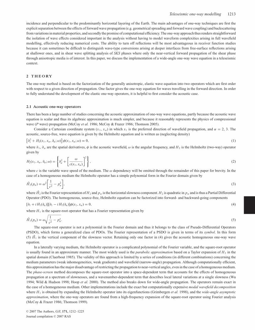
incidence and perpendicular to the predominantly horizontal layering of the Earth. The main advantages of one-way techniques are first the

explicit separation between the effects of forward wave propagation (e.g. geometrical spreading and forward wave coupling) and backscattering

from variations in material properties, and secondly the promise of computational efficiency. The one-way approach thus renders straightforward

the isolation of wave effects considered important in the analysis without having to model waveform complexities arising in full wavefield

modelling, effectively reducing numerical costs. The ability to turn off reflections will be most advantageous in receiver function studies

because it can sometimes be difficult to distinguish wave-type conversions arising at deeper interfaces from free-surface reflections arising

at shallower ones, and in shear wave splitting analysis of SKS phases where only the near-vertical forward propagation of the shear phase

through anisotropic media is of interest. In this paper, we discuss the implementation of a wide-angle one-way wave equation in a teleseismic

context.

2 T H E O RY

The one-way method is based on the factorization of the generally anisotropic, elastic wave equation into two operators which are first order

with respect to a given direction of propagation. One factor gives the one-way equation for waves travelling in the forward direction. In order

to fully understand the development of the elastic one-way operators, it is helpful to first consider the acoustic case.

2.1 Acoustic one-way operators

There has been a large number of studies concerning the acoustic approximation of one-way wave equations, partly because the acoustic wave

equation is scalar and thus its algebraic approximation is much simpler, and because it reasonably represents the physics of compressional

wave (P wave) propagation (McCoy et al. 1986; McCoy & Frazer 1986; Thomson 2005).

Consider a Cartesian coordinate system (x 1, x α) in which x1 is the preferred direction of wavefield propagation, and α = 2, 3. The

acoustic, source-free, wave equation is given by the Helmholtz equation and is written as (neglecting density)[∂2

1 + H2(x1, xα, ∂α; ω)]φ(x1, xα; ω) = 0, (1)

where ∂ 1, ∂α are the spatial derivatives, φ is the acoustic wavefield, ω is the angular frequency, and H 2 is the Helmholtz (two-way) operator

given by

H2(x1, xα, ∂α; ω) ={

∂2α +

[ω

c(x1, xα)

]2}

, (2)

where c is the variable wave speed of the medium. The ω dependency will be omitted through the remainder of this paper for brevity. In the

case of a homogeneous medium the Helmholtz operator has a simple polynomial form in the Fourier domain given by

H̃ 2(pα) = ω2

[1

c2− p2

α

], (3)

where H̃ 2 is the Fourier representation of H 2 and pα is the horizontal slowness component. H 2 is quadratic in pα and is thus a Partial Differential

Operator (PDO). The homogeneous, source-free, Helmholtz equation can be factorized into forward- and backward-going components

[∂1 + i H1(∂α)][∂1 − i H1(∂α)]φ(x1, xα) = 0, (4)

where H 1 is the square-root operator that has a Fourier representation given by

H̃ 1(pα) = ω

√1

c2− p2

α. (5)

The square-root operator is not a polynomial in the Fourier domain and thus it belongs to the class of Pseudo-Differential Operators

(PSDO), which forms a generalized class of PDOs. The Fourier representation of a PSDO is given in terms of its symbol. In this form

(5) H̃ 1 is the vertical component of the slowness vector. Retaining only one factor in (4) gives the acoustic homogeneous one-way wave

equation.

In a laterally varying medium, the Helmholtz operator is a complicated polynomial of the Fourier variable, and the square-root operator

is usually found in an approximate manner. The most widely used is the parabolic approximation based on a Taylor expansion of H 2 in the

spatial domain (Claerbout 1985). The validity of this approach is limited by a series of conditions (in different combinations) concerning the

medium parameters (weak inhomogeneities, weak gradients) and wavefield (narrow-angle) propagation. Although computationally efficient,

this approximation has the major disadvantage of restricting the propagation to near-vertical angles, even in the case of a homogeneous medium.

The phase-screen method decomposes the square-root operator into a space-dependent term that accounts for the effects of homogeneous

propagation at a spectrum of slownesses, and a wavenumber-dependent term that describes local lateral variations at a single slowness (Wu

1994; Wild & Hudson 1998; Hoop et al. 2000). The method also breaks down for wide-angle propagation. The operators remain exact in

the case of a homogeneous medium. Other implementations include the exact but computationally expensive modal wavefield decompositionwhere H 1 is obtained by expanding the Helmholtz operator into its eigenfunctions (Grimbergen et al. 1998), and the wide-angle asymptoticapproximation, where the one-way operators are found from a high-frequency expansion of the square-root operator using Fourier analysis

(McCoy & Frazer 1986; Thomson 1999).

C© 2007 The Authors, GJI, 171, 1212–1225


1214 P. Audet, M. G. Bostock and J.-P. Mercier

All the ideas presented above can be generalized to the elastic and generally anisotropic one-way (vector) wave equation (e.g. Thomson

1999). For example, a parabolic approximation has been successfully implemented to model waveform distortions due to elastic heterogeneity

and anisotropy at a low computational cost (Angus et al. 2004; Angus 2005). Thomson (1999) also derived an expression for the wide-angle

propagation of elastic wavefields based on plane-wave (Fourier) decomposition and a high-frequency approximation of the square-root operator.

The leading-order term in frequency has a simple form in terms of the eigenpolarizations and slownesses for plane waves, and describes

the forward phase propagation and coupling of the wave components. Higher-order terms describing the scattering due to inhomogeneities,

and sometimes referred to as energy-flux normalization terms (e.g. Chapman 2004), are left unexploited. An acoustic implementation of the

wide-angle, one-way method showed that physically motivated approximations greatly improved upon the numerical efficiency (Thomson

2005). It was found that higher-order terms are of utmost importance for the proper description of the differential transmission of energy across

an interface. Here we build upon these findings and develop the elastic analogue of the acoustic implementation. The necessary theoretical

background of the elastic wide-angle, one-way wave equation is provided in detail in the paper by Thomson (1999). A brief summary is

presented in the next subsection.

2.2 Elastic one-way operators

The source-free elastic one-way wave equation for waves travelling in the forward (x1) direction in a homogeneous medium is given by

[∂1 − iωD(∂α)]u(x1, xα) = 0, (6)

where D =GP1G−1 will be termed the propagator matrix, the 3 × 3 matrices G and P1 are, respectively, the three-column eigendisplacements

of the forward going waves and the diagonal matrix of corresponding eigenvalues of p1, and u is the three-component displacement vector

(Thomson 1999). The propagator matrix is the square-root operator, solution to the factorization of the homogeneous wave equation, and is

the equivalent of eq. (5) for an elastic medium. The theory described herein takes into account the full elastic tensor and thus readily allows for

waveform modelling through the most general anisotropic media. The propagator matrix properly describes the phase shift propagation and

mode coupling between the different wave types composing the forward-going wavefield. No assumptions have been made in the derivation

of eq. (6), and hence it is exact.When inhomogeneities are present, the differential operators are represented in the Fourier domain with respect to the transverse

coordinates, where Fourier analysis is used to obtain an approximate solution. The factorization of the inhomogeneous wave equation requires

the solution of the square-root operator which is a PSDO that has a Fourier representation in terms of its symbol. In the remainder of the

paper we will adopt the shorthand sym[D(xα, ∂α)] = D̃(xα, pα) ≡ D(xα, pα), and omit the x1 dependency unless otherwise specified. Since

an exact representation of the symbol of the root operator is difficult to obtain, a high-frequency asymptotic expansion is commonly applied

(Thomson 1999). This approximation still allows for finite-frequency scattering because the signal is band-limited in practice, but restricts

the length scales for observing material heterogeneity (McCoy et al. 1986). Only the first two terms of the expansion are retained and the

one-way equation is written (see Appendix A)

∂1u(xα) =(

ω

2π

)2 ∫ ∫ [iωD0(xα, pα) + iD1(xα, pα) + O(ω−1)

]exp[iω(xα − yα)pα]u(yα) dyα dpα. (7)

Thomson (1999) shows that the leading-order term in frequency is given by the propagator matrix derived in the homogeneous case

D0(xα, pα) = G(xα, pα)P1(xα, pα)G(xα, pα)−1,

extended by a decomposition/recomposition over transverse plane waves. To recover the wavefield, the leading-order one-way wave equation

(cf. eq. 7, omitting D1) performs a number of operations: (1) the first integration over yα decomposes u(yα) into local plane waves; (2) the

matrix G−1 resolves the displacement into quasi-P, and quasi-S1, S2 plane modes; (3) the diagonal matrix P1 defines the rate of progression of

each local plane mode along x1; (4) the matrix G reconstitutes the total plane wavefield after a step in that direction and (5) the integration over

pα reconstitutes the wave fronts. In this form the wide-angle propagator correctly models geometric ray theory, Maslov- and Kirchhoff-like

representations of the elastic wavefield, because no restriction is made concerning the range of slownesses allowed (Thomson 1999; Angus

2007). However, the solution of (7) requires time-consuming integrations in both spatial and wavenumber (or slowness) domains. Thomson

(2005) showed that physically motivated assumptions can greatly improve upon numerical efficiency, as described in the next subsection.

The second-order term represents the energy-flux normalization term that properly describes the amplitude scaling due to the lateral

and depth dependent variations of the medium parameters. The exact form of this term requires the inversion of matrices and an increase in

computational costs. We derive in Appendix A an approximate factor that takes the form

D1(xα, pα) ≈ − i

2G(xα, pα)

{[C11(xα)P1(xα, pα)]−1 ∂1 [C11(xα)P1(xα, pα)]

}G(xα, pα)−1, (8)

where C11 is, in the special case of isotropy, a diagonal matrix given by the inverse wave speeds of the wave modes (see Appendix A). The

approximate amplitude scaling factor (8) neglects the effects due to gradients of the medium parameters in the transverse direction, and is

based on the narrow-angle approximation. However the one-way operators still describe lateral gradient effects through the dependence of all

the terms on x α . This form was also chosen because it is implemented in a straightforward manner, as described in the following subsections.

C© 2007 The Authors, GJI, 171, 1212–1225



2.3 Practical considerations

2.3.1 Higher order extrapolation

The one-way eq. (7) defines the derivative of the wavefield in the preferred direction of propagation. The leading term can be differentiated

with respect to x1 to yield the second derivative ∂21u accurate to within the one-way approximation (Thomson 1999). The extended propagator

is then expanded as (eq. 5.9 of Thomson 1999)

ε∂1u(xα) + 1/2ε2∂21 u(xα) =

(ω

2π

)2 ∫ ∫ [iωD0(xα, pα)ε + 1/2iω∂1D0(xα, pα)ε2 − 1/2ω2D2

0(xα, pα)ε2]

exp[iω(xα − yα)pα]u(yα) dyα dpα + O(ε3). (9)

A simplification occurs if the propagator is evaluated at the midpoint x 1 + 1/2 ε ≡ x ε , and after re-introducing the x1 dependency the

one-way wave equation can be written

u(x1 + ε, xα) =(

ω

2π

)2 ∫ ∫G(xε, xα, pα) exp[iωP1(xε, xα, pα)ε] · G−1(xε, xα, pα) exp[iω(xα − yα)pα]u(x1, yα) dyαdpα + O(ε3). (10)

It can be seen from eq. (10) that the conversion of wave types across an interface are taken up by a form of boundary condition

for displacements through the product G−1(x +ε)G(x −ε). If the material properties vary across the interval [x −ε , x +ε], this matrix product

introduces off-diagonal elements and generates converted waves that are then propagated with the exponential phase term.

In the derivation of the above expression (10), it was assumed that lateral gradients are small, and that the stepsize ε is small enough

for the Taylor expansion to be valid. However, Thomson (2005) suggests that larger stepsize may be used in practice, because the form (10)

corresponds to the exact separable solution in a homogeneous medium. The stepsize can then be chosen to densely sample the medium where

vertical and lateral inhomogeneities exist, and remain coarse elsewhere.

2.3.2 Natural interpolation

In the form (10), the one-way wave equation still appears to require a prohibitive amount of computation, because the Fourier synthesis

necessitates (1) the decomposition of the wavefield into Fourier (plane waves) components over N lateral x α gridpoints (first use of the FFT

with N log2 N operations), and (2) the formation of a unique propagator, or the associated eigenvectors/eigenvalues matrices (G, P1, G−1),

and inverse transform at each lateral x α gridpoint (N use of the FFT, N 2 log2 N operations).

The propagation of the wavefield thus requires N + 1 FFT calls at each frequency. To reduce the costs of computations, a key observation

(Thomson 2005) is made concerning the form of the one-way wave equation. For a laterally homogeneous (layered) model, the propagator

obviously needs only be evaluated at a single lateral gridpoint, and so the modelling requires only two calls to the FFT to describe the

propagation. If the model consists of only a few homogeneous regions described by M < N special points (or nodes) on the lateral grid, and

if in between points are interpolated to give smooth wave speed gradients, the propagator needs only be evaluated at those M points. This

yields M coverings of the entire lateral grid, and the second integral becomes a weighted sum of the M partial contributions to the wavefield,

where the weights are the interpolation coefficients calculated for the earth model. The number of FFT required to describe the propagation

of the wavefield is thus reduced to M , and hence necessitates MN log2 N operations, that is, computational costs are linearly proportional to

M . See Thomson (2005) for details on computation. We note that the laterally varying regions represent variations of the full elastic tensor,

and thus include variations in anisotropic parameters as well as variations in isotropic wave speeds.

2.3.3 Scattering operators

Near vertical reflection/transmission (R/T) at horizontal boundaries can be addressed directly in the one-way approach. The transmission

operator is simply the forward square-root operator given by (7). Explicitly, the transmitted wavefield is calculated by including the second

order term D1 in the asymptotic expansion of the square-root operator, D, and takes the form

uT (x1 + ε, xα) =(

ω

2π

)2 ∫ ∫G(xε, xα, pα)T(xε, xα, pα) exp[iωP1(xε, xα, pα)ε]G−1(xε, xα, pα)

exp[iω(xα − yα)pα]u(x1, yα) dyα dpα, (11)

where the energy-flux term is obtained by the integration of (8) over a small step ε in the forward direction following the procedure described

previously, and is written

T(xε, xα, pα) =√

[C11(x+ε, xα)P1(x+ε, xα, pα)]−1 [C11(x−ε, xα)P1(x−ε, xα, pα)]. (12)

The reflection operator is not derived explicitly because the 3 × 3 formulation neglects the coupling between forward and backward

going waves. However to the same order of approximation we can use the local plane-wave coefficients for reflection computed using the

material properties across the interface at lateral position x α and slowness pα , because they represent the higher order terms in the asymptotic

expansion of the corresponding pseudo-differential operators (McCoy et al. 1986; McCoy & Frazer 1986).

C© 2007 The Authors, GJI, 171, 1212–1225



The natural interpolation idea also applies to the scattering operators since the single-interface R/T is asymptotically local (Thomson

2005). The extension to a sequence of laterally inhomogeneous layers relates closely to the theory of invariant embedding (Kennett 1983),

where the exact reflection and transmission response is calculated for a stack of homogeneous layers. From an implementation perspective,

the first-order effects of scattering are obtained by making two passes through the model; one in the forward direction and a second in the

reverse direction. The reflection coefficients are stored during the first pass and added to the wavefield on the second pass (Thomson 2005).

Free surface multiples can be included in the wavefield by calculating the local plane wave free surface reflection coefficients and applying

them to the wavefield at the surface on the first pass. In the second pass the reflected wavefield at the surface is taken as the initial wavefield and

marched in the reverse direction. On the third pass the reflection coefficients calculated on the second pass are added to the initial wavefield.

2.3.4 2.5-D modelling

Although the wide-angle one-way formulation allows for waveform modelling through 3-D media, we restrict our applications to 2-D models

with invariant material properties in the perpendicular direction. For planar incident wavefields there is a single 2-D horizontal slowness

for any individual source. We can thus model 3-D propagation through 2-D media by giving a harmonic dependence to the wavenumber

component of the incident wavefield in the perpendicular direction because it will scatter independently from the in-plane components.

3 S Y N T H E T I C E X A M P L E S

3.1 1-D crustal structure

This example serves as a benchmark for the one-way implementation of teleseismic wave propagation with the aim of validating the amplitude

correction term (12) and first-order scattering by invariant embedding described in the previous section. The 1-D model consists of a 36 km

layer with typical crustal properties (V p = 6.55 km s−1, V s = 3.70 km s−1, ρ = 2800 kg m−3) overlying a mantle-like half-space (V p =8.10 km s−1, V s = 4.50 km s−1, ρ = 3500 kg m−3). The model has a total vertical extent of 100 km, and the vertical spacing in the extrapolation

is varied from 15 km within the homogeneous regions, to 250 m near the discontinuity. Because the model is laterally homogeneous, the

natural interpolation idea states that the model needs only be sampled at one lateral gridpoint. Wavefield extrapolation is still carried out on the

2-D grid and seismograms are obtained at each lateral gridpoint. The lateral extent is 384 km with 3 km spacing. We selected the seismogram

at the centre of the grid to compare with the reference solution.

The input wavefield is a positively polarized plane P-wave Ricker pulse coming from below with a dominant wavelength of 10 km (at

mantle P velocities) and a horizontal slowness of 0.08 s km−1, which is the maximum limit usually encountered in teleseismic studies (Bostock

1998). Time spacing is taken as 0.25 s and 129 frequencies are used. The propagated one-way wavefield is compared with a reference solution

calculated with the reflectivity technique (Kennett 1983; Thomson 1996), which calculates the exact R/T response for a vertical stack of plane

homogeneous layers.

Fig. 1 shows the horizontal and vertical component seismograms. The one-way results reproduce the P to S wave conversion generated

from the velocity contrast at the Moho, termed P mS , and the free-surface reverberations and conversions of the different phases P PmP, P SmP +P PmS , P SmS . The modelling reproduces the relative arrival times exactly, although the amplitudes are not fully corrected by our approximate

amplitude normalizing factor (e.g. P SmS).

This example demonstrates one of the limits of the wide-angle approach. Increasingly accurate results are found for wavefields propagating

at smaller slownesses. To illustrate this effect we calculated the relative difference in amplitude for increasing slowness for both the horizontal

and vertical components (Fig. 2). The amplitude difference increases quasi linearly with increasing slowness. The amplitude difference is lower

for the horizontal component and it reaches zero at normal incidence. The amplitude difference reaches 4 per cent for the vertical component

at a slowness of 0.08. This fit is reasonable considering the large horizontal slowness of the incident plane wave, the large velocity contrast,

and the level of approximation in obtaining the amplitude correction term (see Appendix A). Note that computation cost is independent of

slowness.

Computation time: ∼10 s using single precision Intel FC compiler on a 2.2 GHz AMD Athlon(tm) 64 processor.

3.2 2-D subduction model

The simple subduction model consists of a downgoing oceanic lithospheric crust and mantle, overriding continental crust and mantle, and

sublithospheric oceanic mantle. The geometry and velocities are based on a simplification of the Cascadia subduction zone model of McNeill

(2005) (Fig. 3). The oceanic crust is defined with a thickness of approximately 6 km. The continental Moho is taken at a depth of 37 km at

the eastern edge of the study area. The subduction zone model is shown as grey shaded contours in Fig. 3. The model is defined on a 360 ×110 km2 Cartesian grid. The lateral and vertical node spacings are equal to 500 m, or about 20 points per dominant wavelength of the initial

P wave in the subslab mantle. Material properties are defined in Table 1. The same geometry is used in the one-way and reference calculations.

The reference solution is calculated using the pseudo-spectral method of Kosloff et al. (1984), which calculates the spatial derivatives

of the full wave equation with the use of the Fast Fourier Transform, instead of by differencing (Finite-Difference) or through interpolation

C© 2007 The Authors, GJI, 171, 1212–1225



−0.6

−0.4

−0.2

0.0

0.2

0.4

0.6

0.8

1.0

1.2

Ve

rtic

al d

isp

lace

me

nt

0 5 10 15 20 25 30

Time (s)

One–Way

RMatrix

PmS PPmP

PSmP +PPmS

PSmS

−0.3

−0.2

−0.1

0.0

0.1

0.2

0.3

0.4

0.5

0.6

0.7

Ho

rizo

nta

l d

isp

lace

me

nt

0 5 10 15 20 25 30

Time (s)

One–Way

RMatrix

PmS

PPmP

PSmP +PPmS PSmS

Figure 1. Comparison of the one-way simulations with the reflectivity technique. (Top) Vertical component seismograms of an initial unit-normalized P-wave

Ricker pulse with a slowness of 0.08 s km−1. (Bottom) Horizontal component seismograms. We artificially introduced a time offset of 0.25 s to visually

compare the one-way results with the reference solution. The one-way results properly reproduce the Moho conversion (PmS) and the free surface multiples

of the different phases (P PmP, P PmS , P SmP, P SmS) and the exact arrival times, although the amplitudes are not fully corrected by the approximate one-way

normalizing factor.

0.000

0.005

0.010

0.015

0.020

0.025

0.030

0.035

0.040

Accu

racy

0.00 0.02 0.04 0.06 0.08

Slowness [s/km]

Vertical

Horizontal

Figure 2. Accuracy of the energy-flux normalization term versus slowness. Grey and black curves show the relative amplitude difference between one-way

simulations and reflectivity technique for the vertical and horizontal components, respectively. The accuracy decreases for increasing slowness, which is expected

due to the narrow-angle assumption in the derivation of the energy-flux term (see Appendix).

functions (Finite-Element). Time derivatives are approximated by differencing and the time spacing is taken to 0.02 s with a total of 1500

increments. The pseudo-spectral method is able to accurately resolve frequencies up to 3.6 Hz. The initial wavefield is a normally incident

plane P-wave Ricker pulse with a dominant wavelength of 10 km at subslab mantle P velocity.

Although larger vertical stepsizes in the one-way method can be specified where the material properties in the vertical direction are

slowly varying, we maintained the same regular spacing to facilitate direct comparison with the reference solution. The lateral model sampling

is specified by the layer discontinuities on a cross-section profile of the model at a given depth. The wavefield is interpolated between adjacent

C© 2007 The Authors, GJI, 171, 1212–1225



0

25

50

75

100

Depth

[km

]

50 100 150 200 250 300 350

Horizontal distance [km]

Figure 3. 2-D subduction zone model defining the geometry of the structural elements: subducting oceanic slab comprising the crust and lithospheric mantle,

the sublithospheric oceanic upper mantle, and the overriding continental crust and upper mantle. Velocities are defined in Table 1.

Table 1. Material properties of the structural elements composing the 2-D subduction

zone model.

Structural element P velocity (km s−1) S velocity (km s−1) Density (kg m−3)

Suboceanic mantle 7.7 4.5 3190

Oceanic slab mantle 8.1 4.6 3340

Oceanic slab crust 6.8 3.9 2900

Subcontinental mantle 7.5 4.1 3260

Continental crust 6.4 3.6 2770

model points as permitted by the natural interpolation idea. One-way extrapolation is performed using the exponential extrapolator for

129 frequencies, with a final seismogram time increment of 0.25 s. In this modelling only the first pass through the model is computed to

capture the essential features of single-scattering and avoid the cluttering of the images due to a high degree of model complexity.

Fig. 4 shows the comparison of horizontal component seismograms from (a) the one-way and (b) the pseudo-spectral method. Amplitudes

are scaled according to unit-normalized initial P-wavefield. Four major features are present in both simulations: (1) the direct transmitted

P arrival refracted at the dipping Moho that disappears beneath normal continental lithosphere; (2) the mixed polarity P S conversions at the

various dipping interfaces and (3) the bleeding tails of the wavefields due to artificial vertical discontinuities at the edges of the box and Fourier

wrap-around effects. Another noteworthy feature seen in the seismograms is the diffraction pattern (4) caused by the point scatterer at the tip of

the mantle wedge, although this feature seems to have a longer duration in the pseudo-spectral synthetics. Moreover the one-way simulations

do not reproduce the wave fronts associated with the internal reflections of the direct P wave and converted S waves (dipping positive and

negative pulses east of km 250, at 14 s and onwards) bouncing off the multiple slab interfaces beneath continental lithosphere, since reflections

have been neglected in this realization. The pseudo-spectral simulation shows further backscattering effects at later times that we chose not to

model with the one-way algorithm. Those are caused by artificial reflections at the free surface due to a velocity contrast between surface and

bottom velocities of the model box. Apart from those later effects, the agreement between the two methods for the forward-scattered portion

of the wavefield is remarkably good considering the level of approximation of the one-way algorithm and the complexity of the velocity

model.

Fig. 5 shows wiggle plots of both horizontal and vertical component seismograms at discrete horizontal locations. Horizontal-component

one-way synthetics are less noisy than the pseudo-spectral results due to (1) the absence of internal reflections in the one-way modelling,

and (2) larger numerical instabilities in the pseudo-spectral algorithm caused by the discrete lateral grid sampling. The main features seen

in horizontal-component seismograms is discussed above. The vertical-component seismograms show the horizontal moveout of the first

arrival due to higher velocities beneath the subducting lithosphere, compared to lower velocities beneath the continental lithosphere. From

6 s onwards the amplitudes are scaled by a factor of 10 to emphasize the finer details of the seismograms. Very low-amplitude free-surface

reflections are again observed at ∼9 s on the pseudo-spectral seismograms that are absent from the one-way simulations. Reflections from

the vertical boundary of the model box appear in both cases although the amplitudes vary between the two methods (e.g. traces 18 and 19).

Absorbing one-way boundary conditions could in theory be implemented to avoid artificial reflections from vertical boundaries (Clayton &

Engquist 1977). An alternative procedure is to extend the model horizontally with constant values outside the rectangle box such that the

artefacts arrive at much later times and do not contaminate the synthetic wavefields. We apply this procedure in the next section for modelling

real data.

Note that non-vertically incident waves can be modelled in both cases with similar levels of accuracy. Normal incidence was chosen

because the waveforms are more easily interpreted in terms of scattering due to structure heterogeneity.

Computation time: one-way ∼15 min using single precision Intel FC compiler on a 2.2 GHz AMD Athlon(tm) 64 processor; pseudo-

spectral about the same as the one-way method on the same machine.

C© 2007 The Authors, GJI, 171, 1212–1225



0

5

10

15

20

25

30

Tim

e [s]

0 50 100 150 200 250 300 350

Horizontal Distance [km]

3

31

2

4

−0.05 0.00 0.05

5

10

15

20

25

30

Tim

e [s]

50 100 150 200 250 300 350

Horizontal Distance [km]

3

31

2

4

5

−0.05 0.00 0.05

Figure 4. Horizontal-component synthetic wavefields calculated using the one-way algorithm (top) and the pseudo-spectral method (bottom). Colorbar shows

the amplitude normalized to the initial incident P-wave. Only one pass is included in the modelling and the seismograms show zeroth-order scattering effects.

The initial wavefield is a normally incident plane wave Ricker pulse with a dominant wavelength of 10 km. Four main features are common to both simulations:

(1) positive P S conversion from the dipping Moho; (2) mixed polarities P S conversions from the various interfaces of the subducting slab; (3) diffraction

patterns associated with edge discontinuities and Fourier wrap-around effects and (4) diffracted wave fronts caused by the point scatterer at the tip of the mantle

wedge. The later arrivals (5) seen in the pseudo-spectral simulation are caused by artificial reflections due to a velocity contrast between the surface and bottom

velocities of the model box. The pseudo-spectral simulations further show multiple internal reflections beneath normal continental Moho. Faint arrivals at t =0–15 s at 100–270 km distance in the one-way synthetics are due to wrap-around effects from time-domain Fourier reconstruction.

3.3 Remarks on computational efficiency

In our demonstration no attempt has been made to optimize the numerical efficiency of the algorithm, that is, we kept a regular grid and only

applied the wavefield interpolation idea. The flexibility offered by using variable stepsizes in the forward direction, which would most improve

upon the numerical efficiency, was not exploited to retain highest possible accuracy. Even so, the one-way algorithm performs equally fast

as the pseudo-spectral technique. As intuition suggests, the computational improvements will be most significant if the contrasts in material

properties in the transverse and vertical directions are small (Thomson 2005).

4 A P P L I C AT I O N T O DATA F RO M N W C A N A DA

A seismic array composed of nearly 60 broad-band instruments with ∼35 km spacing was recently deployed in northwestern Canada as part of

the IRIS- PASSCAL/LITHOPROBE CAnada NOrthwest Experiment (CANOE) for a period of 15–27 months. A subset of the array stretching

over the Wopmay orogen was more densely sampled with station spacing of ∼15 km (Fig. 6). This subset of 20 stations allowed teleseismic

study of a Proterozoic fossil subduction zone previously characterized by LITHOPROBE (SNORCLE) reflection/refraction surveys (Cook &

Erdmer 2005). Fig. 6 shows the location and events used in the study. Data were processed using standard receiver function techniques (Bostock

1998). Receiver functions are source-normalized seismograms obtained by deconvolving the P component from the SV (shear radial) and SH

C© 2007 The Authors, GJI, 171, 1212–1225



0 5 10 15 20 25 30

0

18

36

54

72

90

108

126

144

162

180

198

216

234

252

270

288

306

324

342

Time [s]

Horizonta

l dis

tance [km

]

Horizontal component

0 5 10 15 20 25 30

0

18

36

54

72

90

108

126

144

162

180

198

216

234

252

270

288

306

324

342

Time [s]

Horizonta

l dis

tance [km

]

Vertical component

Figure 5. Wiggle plots of horizontal (left-hand side) and vertical (right-hand side) component seismograms obtained with the one-way (black lines) and the

pseudo-spectral (grey lines) methods. Horizontal-component one-way seismograms are less noisy than the pseudo-spectral results, and the main arrivals are

coherent over the whole time range. Vertical-component seismograms show a moveout due to lower velocities beneath normal continental mantle. Vertical

amplitudes have been scaled up 10 times starting at 6 s to emphasize the finer details of the seismograms.

Figure 6. Data and station array from the CANOE seismic experiment in northwestern Canada. (left-hand side) Events used in the generation of teleseismic

receiver functions. (right-hand side) Subset of stations used in the analysis composed of 20 stations with ∼15 km spacing.

(shear transverse) components, and characterize the scattering structure of the crust and upper mantle underlying seismic stations. Details of

the methodology and interpretation are described in the paper by Mercier et al. (2007).

Individual receiver functions are ordered from left to right along the profile based on the geographic station locations, and, for individual

stations, on the sampling point of the P S conversions projected onto the west–east directions. Radial- and transverse-component receiver

function images (Fig. 8, bottom two panels) of the subsurface beneath this region shows a complex pattern of seismic discontinuities. The

radial receiver function image (Fig. 8, bottom left-hand side) shows a clear and nearly continuous Moho at ∼4 s, represented by a red pulse

with one significant, 75 km long interruption near the suture at km 150. In the same area, the presence of crustal material dipping into the

mantle is also inferred. The geometry of subduction is better defined, however, on the transverse component image where the subducting plate

is associated with a ∼10 km thick layer exhibiting strong elastic anisotropy. This layer clearly extends from depths of 35 km (∼4 s) at the

suture to at least 70 km (∼9 s), over a distance of 150 km further eastward, with some indication that it dips still more steeply thereafter to

depths of >120 km. A 1 − θ correction has been applied to the transverse component receiver functions to improve the visual coherence of

the dipping structure (Mercier et al. 2007).

Previous reflection/refraction surveys imaged strong dipping reflectors at the suture between the two terranes down to a depth of ∼60 km

that are interpreted to be a ∼10 km thick subducting crustal layer (Cook & Erdmer 2005). Surprisingly, but quite definitively, the anisotropic

layer imaged with teleseismic receiver functions does not coincide with the crustal reflectors but, rather, parallels that feature. The top of

the anisotropic layer corresponds to the base of the crustal layer, that is, the Moho of the subducting plate. The top of the crustal layer is

not evident in the teleseismic image. The P S conversion from the base of the anisotropic layer exhibits a frequency dependence favouring

C© 2007 The Authors, GJI, 171, 1212–1225



0

25

50

75

100

125

De

pth

[km

]

50 100 150 200 250

Horizontal distance [km]

Figure 7. Subsurface model of northwestern Canada showing the geometry of the dipping layer, represented as a series of 5 thin layers exhibiting a gradual

linear decrease in anisotropy from top to bottom with an average mantle velocity. The maximum amplitude of hexagonal anisotropy is 5 per cent at the top of

the layer and the fast axis of seismic wave speed has a plunge of 51◦ within the plane of the slab and a trend of 54◦ calculated from the north. The plunge and

trend are rotated along the downgoing portion of the slab to account for the layer dip. Subslab mantle and crustal P-velocities are taken to 8.1 and 6.6 km s−1,

and S-velocities are those calculated for a Poisson solid [α = √(3)β]. The subcontinental wedge shows a gradual increase in velocity from 7 to 8.1 km s−1 to

the eastern edge of the model box.

low frequencies which suggests that it is better modelled as a first-order (versus zeroth-order) discontinuity (or linear gradient) in material

properties.

The argument favouring anisotropy versus dipping isotropy deserves some discussion because it provides insights into the nature of the

anomalous structure. Coherent energy on the transverse component is the consequence of lateral heterogeneity, anisotropy, or both. However

the presence of energy on the transverse component directly beneath the horizontal portion of the Moho at distances less than 150 km cannot

be produced by an isotropic interface. The absence of strong conversion from the lower (basal) interface of the dipping layer on the radial

component suggests that average velocities of the layer and the underlying mantle are comparable. Moreover, the azimuthal correction applied

to the transverse component image does not correspond to the signature of an isotropic layer dipping to the east. Note that we were not able

to reproduce the main features on the transverse component using either a low- or high-velocity isotropic layer.

This data set offers a convenient opportunity to test the one-way algorithm for various material properties including heterogeneity,

anisotropy, as well as physical wave phenomena such as frequency-dependent scattering. In order to reproduce the main features of the

receiver functions we model the lithospheric structure as a ∼10 km thick layer of dipping anisotropic material (average V p = 8.1 km s−1)

overlying a homogeneous mantle (V p = 8.1 km s−1, isotropic Poisson material), overlain by a 37 km thick homogeneous crust (V p =6.6 km s−1) (Fig. 7). We model the interruption and dipping of the Moho on the radial component by a subcrustal mantle wedge showing

a linear horizontal gradient in velocity from V p = 7 km s−1 at the suture to 8.1 km s−1 at the eastern boundary. We note that purely linear

horizontal gradients need not be sampled at the same rate as dipping discontinuities, since only two points are necessary to model a linear

gradient. This is reminiscent of the natural interpolation idea described in Section 2.3.2

The first order discontinuity within the slab is modelled as a stack of thin layers showing a decrease from strong (5 per cent) to weak

anisotropy (hexagonal symmetry) from top to bottom. The fast axis of seismic wave speed has a plunge that follows the layer dip and a

trend of 220◦. Note that the natural interpolation idea is applied to the full elastic tensor, and not to the anisotropic parameters (symmetry

axis, strength, etc.). Model discretization is 128 × 220 with spatial sampling of 2 km laterally, and 500 m vertically. Vertical grid spacing is

increased to 5 km in the homogeneous crustal section. The three-component seismograms are picked according to stations location along the

regular 2-D profile.

In order to produce results consistent with the receiver functions, we used the same events (in terms of slownesses and backazimuths) as

input to the algorithm and applied the same processing as the raw data to produce similar receiver functions. As before the initial wavefields

are pure plane P-wave Ricker wavelets with a dominant wavelength of 10 km. Real and synthetic receiver functions are plotted in Fig. (8) in

bottom panels. Traces are filtered between 0.2 and 1.5 Hz.

The dipping anisotropic layer model clearly accounts for the essential features seen in the receiver functions, although finer details are

left unmodelled. The radial component receiver function shows the discontinuous positive P S Moho conversion, and the presence of material

dipping into the mantle. The dipping layer is obviously identified on the transverse component and shows the frequency-dependent signature

of a velocity gradient, in this case a gradient in anisotropy. The implications of this exercise are twofold: (1) the one-way algorithm is able

to reproduce all phenomena related to material heterogeneity, anisotropy, and gradients (2) the presence of dipping anisotropic material at

lithospheric mantle depths suggests that shallow subduction was active in the early Proterozoic and that this process may have helped in the

stabilization of subcontinental mantle root. The latter interpretation is discussed in detail in the paper by Mercier et al. (2007).

5 C O N C L U S I O N

We implement a waveform modelling tool using the elastic one-way wave equation to model wave effects generated by structural heterogeneity

and anisotropy in a teleseismic context. The form of wave propagation (near planar wave fronts) and scattering operators affords a number of

physically motivated approximations to improve upon the computational efficiency of the algorithm. We show through synthetic modelling

that the algorithm is able to reproduce waveforms from a simple 1-D model including free-surface reflections, and a 2-D heterogeneous model.

C© 2007 The Authors, GJI, 171, 1212–1225



Figure 8. Modelled (top panel) and observed (bottom panel) teleseismic receiver functions (RF) of the CANOE seismic experiment. Left-hand panels show

the radial component RF; right-hand panels are the transverse component RF. The same set of slownesses and backazimuths was used to generate the one-way

synthetic data. A butterworth filter is applied to the RF to emphasize frequency-dependent effects. The radial component shows strong signals at <2 s due to

reverberations within the sedimentary cover that are not modelled in the simulations. On the same component, a clear continuous positive (red) pulse associated

with P S conversion at the Moho is visible at ∼4 s with one interruption near a suture between two Palaeo-Proterozoic terranes, and the presence of crustal

material dipping into the mantle. The geometry is better defined, however, on the transverse component where the dipping layer exhibits strong elastic anisotropy

and first-order frequency effects from a gradual decrease in the percentage of anisotropy from top to bottom of the slab. The one-way simulations reproduce

the main features seen in the data.

We then proceed to model data from an array of seismic stations deployed in northwestern Canada that show a dipping layer of anisotropic

material interpreted to be a fossilized Proterozoic subduction structure. We show that the algorithm reproduces the main features of the data.

The wide-angle, elastic one-way algorithm could be used in other teleseismic applications such as SKS splitting analysis in complicated

settings, for example simulating the signature of corner flow behind a subduction front (Levin et al. 2007). Its relatively low computational cost

makes it a good candidate for Monte Carlo inversion of single scattering of teleseismic wavefields. The model implementation and sampling

is readily expanded in three dimensions to simulate wave propagation in more complicated media. These applications will be the focus of

future studies.

A C K N O W L E D G M E N T S

We thank Colin Thomson and Doug Angus for fruitful discussions at various stages of this work. We thank the two reviewers for their thorough

and constructive reviews. This work is supported by the Natural Science and Engineering Research Council of Canada through a Post-Graduate

Scholarship to PA and a Discovery Grant to MGB.

R E F E R E N C E S

Angus, D.A., 2005. A one-way wave equation for modelling seismic wave-

form variations due to elastic heterogeneity, Geophys. J. Int., 162, 882–

898.

Angus, D.A., 2007. True amplitude corrections for a narrow-angle one-way

elastic wave equation, Geophysics, 72, T19–T26.

Angus, D.A., Thomson, C.J. & Pratt, R.G., 2004. A one-way wave equa-

tion for modelling variations in seismic waveforms due to elastic

anisotropy, Geophys. J. Int., 156, 595–614.

Bostock, M.G., 1998. Mantle stratigraphy and evolution of the Slave

province, J. geophys. Res., 103(B9), 21 183–21 200.

Bostock, M.G., Hyndman, R.D., Rondenay, S. & Peacock, S.M., 2002. An

inverted continental Moho and serpentinization of the forearc mantle,

Nature, 417, 536–539.

Chapman, C., 2004. Fundamentals of Seismic Wave Propagation, Cambridge

University Press, Cambridge, UK.

Claerbout, J., 1985. Imaging the Earth’s interior, Blackwell Sci. Publ.,

Oxford, United Kingdom (GBR).

Clayton, R. & Engquist, B., 1977. Absorbing boundary conditions for acous-

tic and elastic wave equations, Bull. seism. Soc. Am., 67, 1529–1540.

Cook, F.A. & Erdmer, P., 2005. An 1800 km cross section of the lithosphere

through the northwestern North American plate: lessons from 4.0 billion

years of Earth’s history, Can. J. Earth Sci., 42(6), 1295–1311.

Grimbergen, J.L.T., Dessing, F.J. & Wapenaar, K., 1998. Modal expansion

of one-way operators in laterally varying media, Geophysics, 63, 995–

1005.

Hoop, M.V.D., Rousseau, J.H.L. & Wu, R.-S., 2000. Generalization of the

phase-screen approximation for the scattering of acoustic waves, WaveMotion, 31, 43–70.

C© 2007 The Authors, GJI, 171, 1212–1225



Kennett, B.L., 1983. Seismic wave Propagation in Stratified Media, Cam-

bridge University Press, Cambridge, UK.

Komatitsch, D. & Tromp, J., 1999. Introduction to the spectral element

method for three-dimensional seismic wave propagation, Geophys. J. Int.,139(3), 806–822.

Kosarev, G., Kind, R., Sobolev, S.V., Yuan, X., Hanka, W. & Oreshin, S.,

1999. Seismic evidence for a detached Indian lithospheric mantle beneath

Tibet, Science, 283, 1306–1309.

Kosloff, D., Reshef, M. & loewenthal, D., 1984. Elastic wave calculations

by the Fourier method, Bull. seism. Soc. Am., 74, 875–891.

Levander, A., 1988. Fourth-order finite-difference P-SV seismograms, Geo-physics, 53(11), 1425–1436.

Levin, V., Okaya, D. & Park, J., 2007. Shear wave birefringence in

wedge-shaped anisotropic regions, Geophys. J. Int., 168, 275–286,

doi:10.1111/j.1365–246X.2006.03224.x.

McCoy, J. & Frazer, L.N., 1986. Propagation modelling based on wave-

field factorization and invariant embedding, Geophys. J. R. astr. Soc., 86,703–717.

McCoy, J., Fishman, L. & Frazer, L.N., 1986. Reflection and transmission at

an interface separating transversely inhomogeneous acoustic half-spaces,

Geophys. J. R. astr. Soc., 85, 543–562.

McNeill, A.F., 2005. Contribution of post-critical reflections to ground mo-

tions from mega-thrust events in the Cascadia subduction zone, Master’sthesis, University of Victoria, BC, Canada.

Mercier, J.-P., Bostock, M.G., Audet, P., Gaherty, J.B., Garnero, E.J. &

Revenaugh, J., 2007. The teleseismic signature of fossil subduction:

Northwestern Canada, J. geophys. Res., submitted.

Poppeliers, C. & Pavlis, G., 2003. Three-dimensional, prestack, plane wave

migration of teleseismic P-to-S converted phases: 2. Stacking multiple

events, J. geophys. Res., 108, 2267, doi:10.1029/2001JB001583.

Thomson, C.J., 1996. Notes on waves in layered media to accompany pro-

gram Rmatrix, in Seismic waves in complex 3-D structures, pp. 147–162,

Department of Geophysics, Charles University.

Thomson, C.J., 1999. The ‘gap’ between seismic ray theory and ‘full’ wave-

field extrapolation, Geophys. J. Int., 137, 364–380.

Thomson, C.J., 2005. Accuracy and efficiency considerations for wide-angle

wavefield extrapolators and scattering operators, Geophys. J. Int., 163,308–323.

Vinnik, L.P., Green, R.W.E. & Nicolaysen, L.O., 1995. Recent deformations

of the deep continental root beneath southern Africa, Nature, 375(6526),

50–52.

Virieux, J., 1986. P-SV wave propagation in heterogeneous media; velocity-

stress finite-difference method, Geophysics, 51(4), 889–901.

Wild, A.J. & Hudson, J.A., 1998. A geometrical approach to the elastic

complex screen, J. geophys. Res., 103, 707–725.

Wu, R.-S., 1994. Wide-angle elastic wave one-way propagation in hetero-

geneous media and an elastic wave complex-screen method, J. geophys.Res., 99, 751–766.

Yuan, X. et al., 2000. Subduction and collision processes in the cen-

tral andes constrained by converted seismic phases, Nature, 408, 958–

961.

Zandt, G., Gilbert, H., Owens, T.J., Ducea, M., Saleeby, J. & Jones, C.H.,

2004. Active foundering of a continental arc root beneath the southern

Sierra Nevada in California, Nature, 431, 41–46.

A P P E N D I X A : A P P RO X I M AT E A M P L I T U D E N O R M A L I Z I N G FA C T O R

In this section, we derive a first order expression for the differential transmission operator of forward going waves, following the same approach

as Thomson (2005). The derivation is based on the propagation through a vertically layered medium, and the expressions are extrapolated to

the case of a laterally varying medium.

The anisotropic elastic wave equation at a single frequency ω in the absence of source is written

∂ j (ci jkl∂kul ) + ω2ρui = 0. (A1)

The elastic tensor cijkl can be written in a more compact form via

(C jk)il = ci jkl .

In a laterally homogeneous medium, eq. (A1) can be simplified to give

C11∂21 u + (Cα1 + C1α)∂α∂1u + ∂1C11∂1u + ∂1C1α∂αu + Cαβ∂α∂βu + ω2ρu = 0. (A2)

This is eq. (2.11) in Thomson (1999) with the terms consisting of lateral derivatives of the elasticity tensor removed. By multiplying on

the left-hand side by C−111 we get

∂21 u + C−1

11 (Cα1 + C1α)∂α∂1u + C−111 Cαβ∂α∂βu + C−1

11 ∂1C11∂1u + C−111 ∂1C1α∂αu + ω2ρC−1

11 u = 0. (A3)

This equation may be exactly rewritten

(∂1 + iD + E)(∂1 − iD)u + i(∂1D)u − D2u + iEDu + Mu = ∂21 u + E∂1u + Mu = 0,

where

M = C−111 (ω2ρI + ∂1C1α∂α + Cαβ∂α∂β ),

E = C−111 [(Cα1 + C1α)∂α + ∂1C11],

and D (x 1, ∂α) is an unknown PDO. If D can be found such that

[D2 − i(∂1D) − iED]u = Mu, (A4)

then (∂ 1 − iD) u = 0 is an exact one-way equation for waves propagating in the forward direction. The Fourier representation of the PDOs Eand M are simply

M = ω2C−111 (ρI − Cαβ pα pβ ) + iωC−1

11 ∂1C1α pα,

E = iωC−111 (Cα1 + C1α) pα + C−1

11 ∂1C11.

C© 2007 The Authors, GJI, 171, 1212–1225



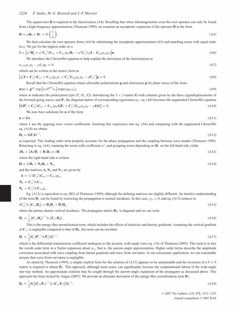
The square-root D is required in the factorization (A4). Recalling that when inhomogeneities exist the root operator can only be found

from a high-frequency approximation (Thomson 1999), we examine an asymptotic expansion of the operator D in the form

D = ωD0 + D1 + O

(1

ω

). (A5)

We then calculate the root operator from (A4) by substituting the asymptotic approximation (A5) and matching terms with equal order

in ω. We get for the highest order in ω

0 = [ω2D2

0 + ω2C−111 (Cα1 + C1α)pαD0 − ω2C−1

11 (ρI − Cαβ pα pβ )]u. (A6)

We introduce the Christoffel equation to help explain the derivation of the factorization as

(ci jkl p j pk − ρδil )gl = 0, (A7)

which can be written in the matrix form as[p2

1I + C−111 (Cα1 + C1α)pα p1 + C−1

11 Cαβ pα pβ − ρC−111

]g = 0. (A8)

Recall that the Christoffel equation relates allowable polarizations g and slownesses p for plane waves of the form:

u(x) = g(m) exp[iωP (m)

1 x1

]exp(iωpαxα), (A9)

where m indicates the polarization type (P, S1, S2). Introducing the 3 × 3 matrix G with columns given by the three eigendisplacements of

the forward-going waves, and P1 the diagonal matrix of corresponding eigenvalues p1, eq. (A8) becomes the augmented Christoffel equation[GP2

1 + C−111 (Cα1 + C1α)pαGP1 + C−1

11 (Cαβ pα pβ − ρI)G] = 0. (A10)

We now have solutions for u of the form

u = Gv, (A11)

where v are the upgoing wave vector coefficients. Inserting this expression into eq. (A8) and comparing with the augmented Christoffel

eq. (A10) we obtain

D0 = GP1G−1, (A12)

as expected. This leading order term properly accounts for the phase propagation and the coupling between wave modes (Thomson 1999).

Returning to eq. (A4), retaining the terms with coefficient ω1, and grouping terms depending on D1 on the left-hand side yields

(D0 + 2A) D1 + D1D0 = iH, (A13)

where the right-hand side is written

H = ∂1D0 + N0D0 + Nα, (A14)

and the matrices A, N0 and Nα are given by

A = 1/2C−111 (Cα1 + C1α)pα,

N0 = C−111 ∂1C11,

Nα = C−111 ∂1C1α pα.

Eq. (A13) is equivalent to eq. (B2) of Thomson (1999), although the defining matrices are slightly different. An intuitive understanding

of the term D1 can be found by restricting the propagation to normal incidence. In this case, pα = 0, and eq. (A13) reduces to

iC−111 ∂1

(C11D′

0

) = D′0D′

1 + D′1D′

0, (A15)

where the primes denote vertical incidence. The propagator matrix D0′ is diagonal and we can write

D′1 = i

2

(C11D′

0

)−1∂1

(C11D′

0

). (A16)

This is the energy-flux normalization term, which includes the effects of elasticity and density gradients. Assuming the vertical gradient

of C11 is negligible compared to that of D0, this term can be rewritten

D′1 = i

2G′ (P′−1

1 ∂1P′1

)G′−1, (A17)

which is the differential transmission coefficient analogous to the acoustic wide-angle wave eq. (14) of Thomson (2005). This term is in fact

the zeroth order term in a Taylor expansion about pα , that is, the narrow-angle approximation. Higher order terms describe the amplitude

correction associated with wave coupling from lateral gradients and wave front curvature. In our teleseismic application, we can reasonably

assume that wave front curvature is negligible.

As stated by Thomson (1999), a simple explicit form for the solution of (A13) appears to be unattainable and the inversion of a 9 × 9

matrix is required to obtain D1. This approach, although more exact, can significantly increase the computational labour of the wide-angle

one-way method. An approximate solution may be sought through the narrow-angle expansion of the propagator as discussed above. This

approach has been treated by Angus (2007). We provide an alternate derivation of the energy-flux normalization term D1:

D1 ≈ i

2G

[(C11P1)−1 ∂1 (C11P1)

]G−1, (A18)

C© 2007 The Authors, GJI, 171, 1212–1225



This form is a crude approximation of the exact form (A13) and neglects possible effects generated from the coupling of waves at

non-vertical incidence in isotropic media. However we adopt this form because it is easily implemented in the wide-angle formulation and

the associated inaccuracies, observed from the comparison of numerical results with a reference solution, are small, as demonstrated by the

numerical examples.

C© 2007 The Authors, GJI, 171, 1212–1225


Teleseismic waveform modelling with a one-way wave equation

Documents

Transcript of Teleseismic waveform modelling with a one-way wave equation