A nonlocal convection–diffusion equation
31
A NONLOCAL CONVECTION-DIFFUSION EQUATION LIVIU I. IGNAT AND JULIO D. ROSSI Abstract. In this paper we study a nonlocal equation that takes into account convective and diffusive effects, ut = J * u - u + G * (f (u)) - f (u) in R d , with J radially symmetric and G not necessarily symmetric. First, we prove existence, uniqueness and continuous dependence with respect to the initial condition of solutions. This problem is the nonlocal analogous to the usual local convection-diffusion equation ut =Δu + b ·∇(f (u)). In fact, we prove that solutions of the nonlocal equation converge to the solution of the usual convection-diffusion equation when we rescale the convolution kernels J and G appropriately. Finally we study the asymptotic behaviour of solutions as t →∞ when f (u)= |u| q-1 u with q> 1. We find the decay rate and the first order term in the asymptotic regime. 1. Introduction In this paper we analyze a nonlocal equation that takes into account convective and diffusive effects. We deal with the nonlocal evolution equation (1.1) u t (t, x)=(J * u - u)(t, x)+(G * (f (u)) - f (u)) (t, x), t> 0,x ∈ R d , u(0,x)= u 0 (x), x ∈ R d . Let us state first our basic assumptions. The functions J and G are nonnegatives and verify R d J (x)dx = R d G(x)dx = 1. Moreover, we consider J smooth, J ∈S (R d ), the space of rapidly decreasing functions, and radially symmetric and G smooth, G ∈S (R d ), but not necessarily symmetric. To obtain a diffusion operator similar to the Laplacian we impose in addition that J verifies 1 2 ∂ 2 ξ i ξ i J (0) = 1 2 supp(J ) J (z )z 2 i dz =1. This implies that J (ξ ) - 1+ ξ 2 ∼|ξ | 3 , for ξ close to 0. Here J is the Fourier transform of J and the notation A ∼ B means that there exist constants C 1 and C 2 such that C 1 A ≤ B ≤ C 2 A. We can consider more general kernels J with expansions in Fourier variables of the form J (ξ ) - 1+ Aξ 2 ∼|ξ | 3 . Since the results (and the proofs) are almost the same, we do not include the details for this more general case, but we comment on how the results are modified by the appearance of A. The nonlinearity f will de assumed nondecreasing with f (0) = 0 and locally Lipschitz continuous (a typical example that we will consider below is f (u)= |u| q-1 u with q> 1). Equations like w t = J * w - w and variations of it, have been recently widely used to model diffusion processes, for example, in biology, dislocations dynamics, etc. See, for example, Key words and phrases. Nonlocal diffusion, convection-diffusion, asymptotic behaviour. 2000 Mathematics Subject Classification. 35B40, 45M05, 45G10. 1
-
Upload
independent -
Category
Documents
-
view
1 -
download
0
Transcript of A nonlocal convection–diffusion equation

A NONLOCAL CONVECTION-DIFFUSION EQUATION
LIVIU I. IGNAT AND JULIO D. ROSSI
Abstract. In this paper we study a nonlocal equation that takes into account convectiveand diffusive effects, ut = J ∗u−u + G ∗ (f(u))− f(u) in Rd, with J radially symmetric andG not necessarily symmetric.
First, we prove existence, uniqueness and continuous dependence with respect to theinitial condition of solutions. This problem is the nonlocal analogous to the usual localconvection-diffusion equation ut = ∆u + b · ∇(f(u)). In fact, we prove that solutions of thenonlocal equation converge to the solution of the usual convection-diffusion equation whenwe rescale the convolution kernels J and G appropriately.
Finally we study the asymptotic behaviour of solutions as t → ∞ when f(u) = |u|q−1uwith q > 1. We find the decay rate and the first order term in the asymptotic regime.
1. Introduction
In this paper we analyze a nonlocal equation that takes into account convective and diffusiveeffects. We deal with the nonlocal evolution equation
(1.1)
{ut(t, x) = (J ∗ u− u) (t, x) + (G ∗ (f(u))− f(u)) (t, x), t > 0, x ∈ Rd,
u(0, x) = u0(x), x ∈ Rd.
Let us state first our basic assumptions. The functions J and G are nonnegatives andverify
∫Rd J(x)dx =
∫Rd G(x)dx = 1. Moreover, we consider J smooth, J ∈ S(Rd), the space
of rapidly decreasing functions, and radially symmetric and G smooth, G ∈ S(Rd), but notnecessarily symmetric. To obtain a diffusion operator similar to the Laplacian we impose inaddition that J verifies
12∂2
ξiξiJ(0) =
12
∫supp(J)
J(z)z2i dz = 1.
This implies thatJ(ξ)− 1 + ξ2 ∼ |ξ|3, for ξ close to 0.
Here J is the Fourier transform of J and the notation A ∼ B means that there exist constantsC1 and C2 such that C1A ≤ B ≤ C2A. We can consider more general kernels J withexpansions in Fourier variables of the form J(ξ)− 1 + A ξ2 ∼ |ξ|3. Since the results (and theproofs) are almost the same, we do not include the details for this more general case, but wecomment on how the results are modified by the appearance of A.
The nonlinearity f will de assumed nondecreasing with f(0) = 0 and locally Lipschitzcontinuous (a typical example that we will consider below is f(u) = |u|q−1u with q > 1).
Equations like wt = J ∗w−w and variations of it, have been recently widely used to modeldiffusion processes, for example, in biology, dislocations dynamics, etc. See, for example,
Key words and phrases. Nonlocal diffusion, convection-diffusion, asymptotic behaviour.2000 Mathematics Subject Classification. 35B40, 45M05, 45G10.
1

2 L. I. IGNAT AND J.D. ROSSI
[2], [4], [6], [7], [10], [13], [14], [20] and [21]. As stated in [13], if w(t, x) is thought of asthe density of a single population at the point x at time t, and J(x − y) is thought of asthe probability distribution of jumping from location y to location x, then (J ∗ w)(t, x) =∫
RN J(y−x)w(t, y) dy is the rate at which individuals are arriving to position x from all otherplaces and −w(t, x) = −
∫RN J(y − x)w(t, x) dy is the rate at which they are leaving location
x to travel to all other sites. This consideration, in the absence of external or internal sources,leads immediately to the fact that the density w satisfies the equation wt = J ∗ w − w.
In our case, see the equation in (1.1), we have a diffusion operator J ∗u−u and a nonlinearconvective part given by G ∗ (f(u))− f(u). Concerning this last term, if G is not symmetricthen individuals have greater probability of jumping in one direction than in others, provokinga convective effect.
We will call equation (1.1), a nonlocal convection-diffusion equation. It is nonlocal sincethe diffusion of the density u at a point x and time t does not only depend on u(x, t) andits derivatives at that point (t, x), but on all the values of u in a fixed spatial neighborhoodof x through the convolution terms J ∗ u and G ∗ (f(u)) (this neighborhood depends on thesupports of J and G).
First, we prove existence, uniqueness and well-possedness of a solution with an initialcondition u(0, x) = u0(x) ∈ L1(Rd) ∩ L∞(Rd).
Theorem 1.1. For any u0 ∈ L1(Rd) ∩ L∞(Rd) there exists a unique global solution
u ∈ C([0,∞);L1(Rd)) ∩ L∞([0,∞); Rd).
If u and v are solutions of (1.1) corresponding to initial data u0, v0 ∈ L1(Rd) ∩ L∞(Rd)respectively, then the following contraction property
‖u(t)− v(t)‖L1(Rd) ≤ ‖u0 − v0‖L1(Rd)
holds for any t ≥ 0. In addition,
‖u(t)‖L∞(Rd) ≤ ‖u0‖L∞(Rd).
We have to emphasize that a lack of regularizing effect occurs. This has been alreadyobserved in [5] for the linear problem wt = J ∗ w − w. In [12], the authors prove that thesolutions to the local convection-diffusion problem, ut = ∆u + b · ∇f(u), satisfy an estimateof the form ‖u(t)‖L∞(Rd) ≤ C(‖u0‖L1(Rd)) t−d/2 for any initial data u0 ∈ L1(Rd)∩L∞(Rd). Inour nonlocal model, we cannot prove such type of inequality independently of the L∞(Rd)-norm of the initial data. Moreover, in the one-dimensional case with a suitable bound on thenonlinearity that appears in the convective part, f , we can prove that such an inequality doesnot hold in general, see Section 3. In addition, the L1(Rd)−L∞(Rd) regularizing effect is notavailable for the linear equation, wt = J ∗ w − w, see Section 2.
When J is nonnegative and compactly supported, the equation wt = J ∗w−w shares manyproperties with the classical heat equation, wt = ∆w, such as: bounded stationary solutionsare constant, a maximum principle holds for both of them and perturbations propagate withinfinite speed, see [13]. However, there is no regularizing effect in general. Moreover, in [8] and[9] nonlocal Neumann boundary conditions where taken into account. It is proved there thatsolutions of the nonlocal problems converge to solutions of the heat equation with Neumannboundary conditions when a rescaling parameter goes to zero.

A NONLOCAL CONVECTION-DIFFUSION EQUATION 3
Concerning (1.1) we can obtain a solution to a standard convection-diffusion equation
(1.2) vt(t, x) = ∆v(t, x) + b · ∇f(v)(t, x), t > 0, x ∈ Rd,
as the limit of solutions to (1.1) when a scaling parameter goes to zero. In fact, let us consider
Jε(s) =1εd
J(s
ε
), Gε(s) =
1εd
G(s
ε
),
and the solution uε(t, x) to our convection-diffusion problem rescaled adequately,
(1.3)
(uε)t(t, x) =
1ε2
∫Rd
Jε(x− y)(uε(t, y)− uε(t, x)) dy
+1ε
∫Rd
Gε(x− y)(f(uε(t, y))− f(uε(t, x))) dy,
uε(x, 0) = u0(x).
Remark that the scaling is different for the diffusive part of the equation J ∗ u− u and forthe convective part G ∗ f(u) − f(u). The same different scaling properties can be observedfor the local terms ∆u and b · ∇f(u).
Theorem 1.2. With the above notations, for any T > 0, we have
limε→0
supt∈[0,T ]
‖uε − v‖L2(Rd) = 0,
where v(t, x) is the unique solution to the local convection-diffusion problem (1.2) with initialcondition v(x, 0) = u0(x) ∈ L1(Rd) ∩ L∞(Rd) and b = (b1, ..., bd) given by
bj =∫
Rd
xj G(x) dx, j = 1, ..., d.
This result justifies the use of the name “nonlocal convection-diffusion problem” when werefer to (1.1).
From our hypotheses on J and G it follows that they verify |G(ξ)− 1− ib · ξ| ≤ C|ξ|2 and|J(ξ)− 1 + ξ2| ≤ C|ξ|3 for every ξ ∈ Rd. These bounds are exactly what we are using in theproof of this convergence result.
Remark that when G is symmetric then b = 0 and we obtain the heat equation in the limit.Of course the most interesting case is when b 6= 0 (this happens when G is not symmetric).Also we note that the conclusion of the theorem holds for other Lp(Rd)-norms besides L2(Rd),however the proof is more involved.
We can consider kernels J such that
A =12
∫supp(J)
J(z)z2i dz 6= 1.
This gives the expansion J(ξ) − 1 + Aξ2 ∼ |ξ|3, for ξ close to 0. In this case we will arriveto a convection-diffusion equation with a multiple of the Laplacian as the diffusion operator,vt = A∆v + b · ∇f(v).
Next, we want to study the asymptotic behaviour as t → ∞ of solutions to (1.1). To thisend we first analyze the decay of solutions taking into account only the diffusive part (thelinear part) of the equation. These solutions have a similar decay rate as the one that holdsfor the heat equation, see [5] and [15] where the Fourier transform play a key role. Usingsimilar techniques we can prove the following result that deals with this asymptotic decayrate.

4 L. I. IGNAT AND J.D. ROSSI
Theorem 1.3. Let p ∈ [1,∞]. For any u0 ∈ L1(Rd) ∩ L∞(Rd) the solution w(t, x) of thelinear problem
(1.4)
{wt(t, x) = (J ∗ w − w)(t, x), t > 0, x ∈ Rd,
u(0, x) = u0(x), x ∈ Rd,
satisfies the decay estimate
‖w(t)‖Lp(Rd) ≤ C(‖u0‖L1(Rd), ‖u0‖L∞(Rd)) 〈t〉− d
2(1− 1
p).
Throughout this paper we will use the notation A ≤ 〈t〉−α to denote A ≤ (1 + t)−α.Now we are ready to face the study of the asymptotic behaviour of the complete prob-
lem (1.1). To this end we have to impose some grow condition on f . Therefore, in the sequelwe restrict ourselves to nonlinearities f that are pure powers
(1.5) f(u) = |u|q−1u
with q > 1.The analysis is more involved than the one performed for the linear part and we cannot
use here the Fourier transform directly (of course, by the presence of the nonlinear term).Our strategy is to write a variation of constants formula for the solution and then proveestimates that say that the nonlinear part decay faster than the linear one. For the localconvection diffusion equation this analysis was performed by Escobedo and Zuazua in [12].However, in the previously mentioned reference energy estimates were used together withSobolev inequalities to obtain decay bounds. These Sobolev inequalities are not available forthe nonlocal model, since the linear part does not have any regularizing effect, see Remark 5.4in Section 5. Therefore, we have to avoid the use of energy estimates and tackle the problemusing a variant of the Fourier splitting method proposed by Schonbek to deal with localproblems, see [17], [18] and [19].
We state our result concerning the asymptotic behaviour (decay rate) of the completenonlocal model as follows:
Theorem 1.4. Let f satisfies (1.5) with q > 1 and u0 ∈ L1(Rd) ∩ L∞(Rd). Then, for everyp ∈ [1,∞) the solution u of equation (1.1) verifies
(1.6) ‖u(t)‖Lp(Rd) ≤ C(‖u0‖L1(Rd), ‖u0‖L∞(Rd)) 〈t〉− d
2(1− 1
p).
Finally, we look at the first order term in the asymptotic expansion of the solution. Forq > (d + 1)/d, we find that this leading order term is the same as the one that appears in thelinear local heat equation. This is due to the fact that the nonlinear convection is of higherorder and that the radially symmetric diffusion leads to gaussian kernels in the asymptoticregime, see [5] and [15].
Theorem 1.5. Let f satisfies (1.5) with q > (d+1)/d and let the initial condition u0 belongsto L1(Rd, 1 + |x|) ∩ L∞(Rd). For any p ∈ [2,∞) the following holds
t− d
2(1− 1
p)‖u(t)−MH(t)‖Lp(Rd) ≤ C(J,G, p, d) αq(t),
where
M =∫
Rd
u0(x) dx,

A NONLOCAL CONVECTION-DIFFUSION EQUATION 5
H(t) is the Gaussian,
H(t) =e−
x2
4t
(2πt)d2
,
and
αq(t) =
〈t〉−12 if q ≥ (d + 2)/d,
〈t〉1−d(q−1)
2 if (d + 1)/d < q < (d + 2)/d.
Remark that we prove a weak nonlinear behaviour, in fact the decay rate and the firstorder term in the expansion are the same that appear in the linear model wt = J ∗ w − w,see [15].
As before, recall that our hypotheses on J imply that J(ξ)− (1− |ξ|2) ∼ B|ξ|3, for ξ closeto 0. This is the key property of J used in the proof of Theorem 1.5. We note that when wehave an expansion of the form J(ξ)− (1−A|ξ|2) ∼ B|ξ|3, for ξ ∼ 0, we get as first order terma Gaussian profile of the form HA(t) = H(At).
Also note that q = (d+1)/d is a critical exponent for the local convection-diffusion problem,vt = ∆v + b · ∇(vq), see [12]. When q is supercritical, q > (d + 1)/d, for the local equation italso holds an asymptotic simplification to the heat semigroup as t →∞.
The first order term in the asymptotic behaviour for critical or subcritical exponents 1 <q ≤ (d+1)/d is left open. One of the main difficulties that one has to face here is the absenceof a self-similar profile due to the inhomogeneous behaviour of the convolution kernels.
The rest of the paper is organized as follows: in Section 2 we deal with the estimates for thelinear semigroup that will be used to prove existence and uniqueness of solutions as well asfor the proof of the asymptotic behaviour. In Section 3 we prove existence and uniqueness ofsolutions, Theorem 1.1. In Section 4 we show the convergence to the local convection-diffusionequation, Theorem 1.2 and finally in Sections 5 and 6 we deal with the asymptotic behaviour,we find the decay rate and the first order term in the asymptotic expansion, Theorems 1.4and 1.5.
2. The linear semigroup
In this section we analyze the asymptotic behavior of the solutions of the equation
(2.1)
{wt(t, x) = (J ∗ w − w)(t, x), t > 0, x ∈ Rd,
w(0, x) = u0(x), x ∈ Rd.
As we have mentioned in the introduction, when J is nonnegative and compactly supported,this equation shares many properties with the classical heat equation, wt = ∆w, such as:bounded stationary solutions are constant, a maximum principle holds for both of them andperturbations propagate with infinite speed, see [13]. However, there is no regularizing effectin general. In fact, the singularity of the source solution, that is a solution to (2.1) withinitial condition a delta measure, u0 = δ0, remains with an exponential decay. In fact, thisfundamental solution can be decomposed as S(t, x) = e−tδ0 + Kt(x) where Kt(x) is smooth,see Lemma 2.1. In this way we see that there is no regularizing effect since the solution w of(2.1) can be written as w(t) = S(t) ∗u0 = e−tu0 +Kt ∗u0 with Kt smooth, which means thatw(·, t) is as regular as u0 is. This fact makes the analysis of (2.1) more involved.

6 L. I. IGNAT AND J.D. ROSSI
Lemma 2.1. The fundamental solution of (2.1), that is the solution of (2.1) with initialcondition u0 = δ0, can be decomposed as
(2.2) S(t, x) = e−tδ0(x) + Kt(x),
with Kt(x) = K(t, x) smooth. Moreover, if u is the solution of (2.1) it can be written as
w(t, x) = (S ∗ u0)(t, x) =∫
RS(t, x− y)u0(y) dy.
Proof. Applying the Fourier transform to (2.1) we obtain that
wt(ξ, t) = w(ξ, t)(J(ξ)− 1).
Hence, as the initial datum verifies u0 = δ0 = 1,
w(ξ, t) = e(J(ξ)−1)t = e−t + e−t(eJ(ξ)t − 1).
The first part of the lemma follows applying the inverse Fourier transform.To finish the proof we just observe that S ∗ u0 is a solution of (2.1) (just use Fubini’s
theorem) with (S ∗ u0)(0, x) = u0(x). �
In the following we will give estimates on the regular part of the fundamental solution Kt
defined by:
(2.3) Kt(x) =∫
Rd
(et(J(ξ)−1) − e−t) eix·ξ dξ,
that is, in the Fourier space,Kt(ξ) = et(J(ξ)−1) − e−t.
The behavior of Lp(Rd)-norms of Kt will be obtained by analyzing the cases p = ∞ andp = 1. The case p = ∞ follows by Hausdorff-Young’s inequality. The case p = 1 follows byusing the fact that the L1(Rd)-norm of the solutions to (2.1) does not increase.
The analysis of the behaviour of the gradient ∇Kt is more involved. The behavior ofLp(Rd)-norms with 2 ≤ p ≤ ∞ follows by Hausdorff-Young’s inequality in the case p = ∞and Plancherel’s identity for p = 2. However, the case 1 ≤ p < 2 is more tricky. In order toevaluate the L1(Rd)-norm of ∇Kt we will use the Carlson inequality (see for instance [3])
(2.4) ‖ϕ‖L1(Rd) ≤ C ‖ϕ‖1− d2m
L2(Rd)‖|x|mϕ‖
d2m
L2(R),
which holds for m > d/2. The use of the above inequality with ϕ = ∇Kt imposes that|x|m∇Kt belongs to L2(Rd). To guarantee this property and to obtain the decay rate for theL2(Rd)-norm of |x|m∇Kt we will use in Lemma 2.3 that J ∈ S(Rd).
The following lemma gives us the decay rate of the Lp(Rd)-norms of the kernel Kt for1 ≤ p ≤ ∞ .
Lemma 2.2. Let J be such that J(ξ) ∈ L1(Rd), ∂ξJ(ξ) ∈ L2(Rd) and
J(ξ)− 1 + ξ2 ∼ |ξ|3, ∂ξJ(ξ) ∼ −ξ as ξ ∼ 0.
For any p ≥ 1 there exists a positive constant c(p, J) such that Kt, defined in (2.3), satisfies:
(2.5) ‖Kt‖Lp(Rd) ≤ c(p, J) 〈t〉−d2(1− 1
p)
for any t > 0.
A NONLOCAL CONVECTION-DIFFUSION EQUATION 7
Remark 2.1. In fact, when p = ∞, a stronger inequality can be proven,
‖Kt‖L∞(Rd) ≤ Cte−δt‖J‖L1(Rd) + C 〈t〉−d/2,
for some positive δ = δ(J).Moreover, for p = 1 we have,
‖Kt‖L1(Rd) ≤ 2
and for any p ∈ [1,∞]‖S(t)‖Lp(Rd)−Lp(Rd) ≤ 3.
Proof of Lemma 2.2. We analyze the cases p = ∞ and p = 1, the others can be easily obtainedapplying Holder’s inequality.
Case p = ∞. Using Hausdorff-Young’s inequality we obtain that
‖Kt‖L∞(Rd) ≤∫
Rd
|et(J(ξ)−1) − e−t|dξ.
Observe that the symmetry of J guarantees that J is a real number. Let us choose R > 0such that
(2.6) |J(ξ)| ≤ 1− |ξ|2
2for all |ξ| ≤ R.
Once R is fixed, there exists δ = δ(J), 0 < δ < 1, with
(2.7) |J(ξ)| ≤ 1− δ for all |ξ| ≥ R.
Using that for any real numbers a and b the following inequality holds:
|ea − eb| ≤ |a− b|max{ea, eb}we obtain for any |ξ| ≥ R,
(2.8) |et(J(ξ)−1) − e−t| ≤ t|J(ξ)|max{e−t, et(J(ξ)−1)} ≤ te−δt|J(ξ)|.Then the following integral decays exponentially,∫
|ξ|≥R|et(J(ξ)−1) − e−t|dξ ≤ e−δtt
∫|ξ|≥R
|J(ξ)|dξ.
Using that this term is exponentially small, it remains to prove that
(2.9) I(t) =∫|ξ|≤R
|et(J(ξ)−1) − e−t|dξ ≤ C〈t〉−d/2.
To handle this case we use the following estimates:
|I(t)| ≤∫|ξ|≤R
et(J(ξ)−1)dξ + e−tC(R) ≤∫|ξ|≤R
dξ + e−tC(R) ≤ C(R)
and
|I(t)| ≤∫|ξ|≤R
et(J(ξ)−1)dξ + e−tC(R) ≤∫|ξ|≤R
e−t|ξ|2
2 + e−tC(R)
= t−d/2
∫|η|≤Rt1/2
e−|η|22 + e−tC(R) ≤ Ct−d/2.
The last two estimates prove (2.9) and this finishes the analysis of this case.

8 L. I. IGNAT AND J.D. ROSSI
Case p = 1. First we prove that the L1(Rd)-norm of the solutions to equation (1.4) doesnot increase. Multiplying equation (1.4) by sgn(w(t, x)) and integrating in space variable weobtain,
d
dt
∫Rd
|w(t, x)| dx =∫
Rd
∫Rd
J(x− y)w(t, y) sgn(w(t, x)) dy ds−∫
Rd
|w(t, x)| dx
≤∫
Rd
∫Rd
J(x− y)|w(t, y)| dx dy −∫
Rd
|w(t, x)| dx ≤ 0,
which shows that the L1(Rd)-norm does not increase. Hence, for any u0 ∈ L1(Rd), thefollowing holds: ∫
Rd
|e−tu0(x) + (Kt ∗ u0)(x)| dx ≤∫
Rd
|u0(x)| dx,
and as a consequence, ∫Rd
|(Kt ∗ u0)(x)| dx ≤ 2∫
Rd
|u0(x)| dx.
Choosing (u0)n ∈ L1(Rd) such that (u0)n → δ0 in S ′(Rd) we obtain in the limit that∫Rd
|Kt(x)|dx ≤ 2.
This ends the proof of the L1-case and finishes the proof. �
The following lemma will play a key role when analyzing the decay of the complete prob-lem (1.1). In the sequel we will denote by L1(Rd, a(x)) the following space:
L1(Rd, a(x)) ={
ϕ :∫
Rd
a(x)|ϕ(x)|dx < ∞}
.
Lemma 2.3. Let p ≥ 1 and J ∈ S(Rd). There exists a positive constant c(p, J) such that
‖Kt ∗ ϕ−Kt‖Lp(Rd) ≤ c(p)〈t〉−d2(1− 1
p)− 1
2 ‖ϕ‖L1(Rd,|x|)
holds for all ϕ ∈ L1(Rd, 1 + |x|).
Proof. Explicit computations shows that
(Kt ∗ ϕ−Kt)(x) =∫
Rd
Kt(x− y)ϕ(y)dy −∫
Rd
Kt(x) dx
=∫
Rd
ϕ(y)(Kt(x− y)−Kt(x)) dy
=∫
Rd
ϕ(y)∫ 1
0∇Kt(x− sy) · (−y) ds dy.(2.10)
We will analyze the cases p = 1 and p = ∞, the others cases follow by interpolation.For p = ∞ we have,
(2.11) ‖Kt ∗ ϕ−Kt‖L∞(Rd) ≤ ‖∇Kt‖L∞(Rd)
∫Rd
|y||ϕ(y)| dy.
A NONLOCAL CONVECTION-DIFFUSION EQUATION 9
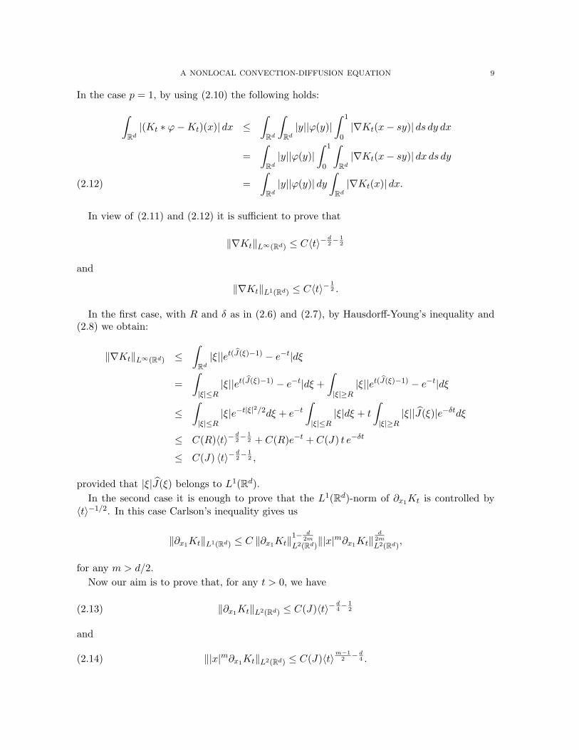
In the case p = 1, by using (2.10) the following holds:∫Rd
|(Kt ∗ ϕ−Kt)(x)| dx ≤∫
Rd
∫Rd
|y||ϕ(y)|∫ 1
0|∇Kt(x− sy)| ds dy dx
=∫
Rd
|y||ϕ(y)|∫ 1
0
∫Rd
|∇Kt(x− sy)| dx ds dy
=∫
Rd
|y||ϕ(y)| dy
∫Rd
|∇Kt(x)| dx.(2.12)
In view of (2.11) and (2.12) it is sufficient to prove that
‖∇Kt‖L∞(Rd) ≤ C〈t〉−d2− 1
2
and
‖∇Kt‖L1(Rd) ≤ C〈t〉−12 .
In the first case, with R and δ as in (2.6) and (2.7), by Hausdorff-Young’s inequality and(2.8) we obtain:
‖∇Kt‖L∞(Rd) ≤∫
Rd
|ξ||et(J(ξ)−1) − e−t|dξ
=∫|ξ|≤R
|ξ||et(J(ξ)−1) − e−t|dξ +∫|ξ|≥R
|ξ||et(J(ξ)−1) − e−t|dξ
≤∫|ξ|≤R
|ξ|e−t|ξ|2/2dξ + e−t
∫|ξ|≤R
|ξ|dξ + t
∫|ξ|≥R
|ξ||J(ξ)|e−δtdξ
≤ C(R)〈t〉−d2− 1
2 + C(R)e−t + C(J) t e−δt
≤ C(J) 〈t〉−d2− 1
2 ,
provided that |ξ|J(ξ) belongs to L1(Rd).In the second case it is enough to prove that the L1(Rd)-norm of ∂x1Kt is controlled by
〈t〉−1/2. In this case Carlson’s inequality gives us
‖∂x1Kt‖L1(Rd) ≤ C ‖∂x1Kt‖1− d
2m
L2(Rd)‖|x|m∂x1Kt‖
d2m
L2(Rd),
for any m > d/2.Now our aim is to prove that, for any t > 0, we have
(2.13) ‖∂x1Kt‖L2(Rd) ≤ C(J)〈t〉−d4− 1
2
and
(2.14) ‖|x|m∂x1Kt‖L2(Rd) ≤ C(J)〈t〉m−1
2− d
4 .

10 L. I. IGNAT AND J.D. ROSSI
By Plancherel’s identity, estimate (2.8) and using that |ξ|J(ξ) belongs to L2(Rd) we obtain
‖∂x1Kt‖2L2(Rd) =
∫Rd
|ξ1|2|et(J(ξ)−1) − e−t|2 dξ
≤ 2∫|ξ|≤R
|ξ1|2e−t|ξ|2dξ + e−2t
∫|ξ|≤R
|ξ1|2dξ +∫|ξ|≥R
|ξ1|2e−2δtt2|J(ξ)|2dξ
≤ C(R)〈t〉−d2− 1
2 + C(R)e−2t + C(J)e−2δtt2
≤ C(J) 〈t〉−d2− 1
2 .
This shows (2.13).To prove (2.14), observe that
‖|x|m∂x1Kt‖2L2(Rd) ≤ c(d)
∫Rd
(x2m1 + · · ·+ x2m
d )|∂x1Kt(x)|2dx.
Thus, by symmetry it is sufficient to prove that∫Rd
|∂mξ1(ξ1Kt(ξ))|2dξ ≤ C(J) 〈t〉m−1− d
2
and ∫Rd
|∂mξ2(ξ1Kt(ξ))|2dξ ≤ C(J) 〈t〉m−1− d
2 .
Observe that
|∂mξ1(ξ1Kt(ξ))| = |ξ1∂
mξ1Kt(ξ) + m∂m−1
ξ1Kt(ξ)| ≤ |ξ||∂m
ξ1Kt(ξ)|+ m|∂m−1ξ1
Kt(ξ)|
and|∂m
ξ2(ξ1Kt)| ≤ |ξ||∂mξ2Kt(ξ)|.
Hence we just have to prove that∫Rd
|ξ|2r|∂nξ1Kt(ξ)|2dξ ≤ C(J) 〈t〉n−r− d
2 , (r, n) ∈ {(0,m− 1), (1,m)} .
Choosing m = [d/2] + 1 (the notation [·] stands for the floor function) the above inequalityhas to hold for n = [d/2], [d/2] + 1.
First we recall the following elementary identity
∂nξ1(e
g) = eg∑
i1+2i2+...+nin=n
ai1,...,in(∂1ξ1g)i1(∂2
ξ1g)i2 ...(∂nξ1g)in ,
where ai1,...,in are universal constants independent of g. Tacking into account that
Kt(ξ) = et(J(ξ)−1) − e−t
we obtain
∂nξ1Kt(ξ) = et(J(ξ)−1)
∑i1+2i2+...+nin=n
ai1,...,inti1+···+in
n∏j=1
[∂jξ1
J(ξ)]ij
and hence
|∂nξ1Kt(ξ)|2 ≤ C e2t(J(ξ)−1)
∑i1+2i2+...+nin=n
t2(i1+···+in)n∏
j=1
[∂jξ1
J(ξ)]2ij .

A NONLOCAL CONVECTION-DIFFUSION EQUATION 11
Using that all the partial derivatives of J decay faster than any polinomial in |ξ|, as |ξ| → ∞,we obtain that ∫
|ξ|>R|ξ|2r|∂n
ξ1Kt(ξ)|2dξ ≤ C(J) e−2δt〈t〉2n
where R and δ are chosen as in (2.6) and (2.7). Tacking into account that J(ξ) is smooth(since J ∈ S(Rd)) we obtain that for all |ξ| ≤ R the following hold:
|∂ξ1 J(ξ)| ≤ C |ξ|
and|∂j
ξ1J(ξ)| ≤ C, j = 2, . . . , n.
Then for all |ξ| ≤ R we have
|∂nξ1Kt(ξ)|2 ≤ C e−t|ξ|2
∑i1+2i2+...+nin=n
t2(i1+···+in)|ξ|2i1 .
Finally, using that for any l ≥ 0∫|ξ|≤R
e−t|ξ|2 |ξ|ldξ ≤ C(R)〈t〉−d2− l
2 ,
we obtain ∫|ξ|≤R
|ξ|2r|∂nξ1Kt(ξ)|2dξ ≤ C(R)〈t〉−
d2
∑i1+2i2+···+nin=n
〈t〉2p(i1,...,id)−r
where
p(i1, . . . , in) = (i1 + · · ·+ in)− i12
=i12
+ i2 + · · ·+ in ≤i1 + 2i2 + . . . nin
2=
n
2.
This ends the proof. �
We now prove a decay estimate that takes into account the linear semigroup applied to theconvolution with a kernel G.
Lemma 2.4. Let 1 ≤ p ≤ r ≤ ∞, J ∈ S(Rd) and G ∈ L1(Rd, |x|). There exists a positiveconstant C = C(p, J, G) such that the following estimate
(2.15) ‖S(t) ∗G ∗ ϕ− S(t) ∗ ϕ‖Lr(Rd) ≤ C〈t〉−d2( 1
p− 1
r)− 1
2 (‖ϕ‖Lp(Rd) + ‖ϕ‖Lr(Rd)).
holds for all ϕ ∈ Lp(Rd) ∩ Lr(Rd).
Remark 2.2. In fact the following stronger inequality holds:
‖S(t) ∗G ∗ ϕ− S(t) ∗ ϕ‖Lr(Rd) ≤ C 〈t〉−d2( 1
p− 1
r)− 1
2 ‖ϕ‖Lp(Rd) + C e−t‖ϕ‖Lr(Rd).
Proof. We write S(t) as S(t) = e−tδ0 + Kt and we get
S(t) ∗G ∗ ϕ− S(t) ∗ ϕ = e−t(G ∗ ϕ− ϕ) + Kt ∗G ∗ ϕ−Kt ∗ ϕ.
The first term in the above right hand side verifies:
e−t‖G ∗ ϕ− ϕ‖Lr(Rd) ≤ e−t(‖G‖L1(Rd)‖ϕ‖Lr(Rd) + ‖ϕ‖Lr(Rd)) ≤ 2e−t‖ϕ‖Lr(Rd).

12 L. I. IGNAT AND J.D. ROSSI
For the second one, by Lemma 2.3 we get that Kt satisfies
‖Kt ∗G−Kt‖La(Rd) ≤ C(r, J)‖G‖L1(Rd,|x|)〈t〉−d2(1− 1
a)− 1
2
for all t ≥ 0 where a is such that 1/r = 1/a+1/p− 1. Then, using Young’s inequality we endthe proof. �
3. Existence and uniqueness
In this section we use the previous results and estimates on the linear semigroup to provethe existence and uniqueness of the solution to our nonlinear problem (1.1). The proof isbased on the variation of constants formula and uses the previous properties of the lineardiffusion semigroup.
Proof of Theorem 1.1. Recall that we want prove the global existence of solutions for initialconditions u0 ∈ L1(Rd) ∩ L∞(Rd).
Let us consider the following integral equation associated with (1.1):
(3.1) u(t) = S(t) ∗ u0 +∫ t
0S(t− s) ∗ (G ∗ (f(u))− f(u))(s) ds,
the functional
Φ[u](t) = S(t) ∗ u0 +∫ t
0S(t− s) ∗ (G ∗ (f(u))− f(u))(s) ds
and the spaceX(T ) = C([0, T ];L1(Rd)) ∩ L∞([0, T ]; Rd)
endowed with the norm
‖u‖X(T ) = supt∈[0,T ]
(‖u(t)‖L1(Rd) + ‖u(t)‖L∞(Rd)
).
We will prove that Φ is a contraction in the ball of radius R, BR, of XT , if T is small enough.Step I. Local Existence. Let M = max{‖u0‖L1(Rd), ‖u0‖L∞(Rd)} and p = 1,∞. Then,
using the results of Lemma 2.2 we obtain,
‖Φ[u](t)‖Lp(Rd) ≤ ‖S(t) ∗ u0‖Lp(Rd)
+∫ t
0‖S(t− s) ∗G ∗ (f(u))− S(t− s) ∗ f(u)‖Lp(Rd) ds
≤ (e−t + ‖Kt‖L1(Rd))‖u0‖Lp(Rd)
+∫ t
02(e−(t−s) + ‖Kt−s‖L1(Rd))‖f(u)(s)‖Lp(Rd) ds
≤ 3 ‖u0‖Lp(Rd) + 6 Tf(R) ≤ 3M + 6 Tf(R).
This implies that‖Φ[u]‖X(T ) ≤ 6M + 12 Tf(R).
Choosing R = 12M and T such that 12 Tf(R) < 6M we obtain that Φ(BR) ⊂ BR.

A NONLOCAL CONVECTION-DIFFUSION EQUATION 13
Let us choose u and v in BR. Then for p = 1,∞ the following hold:
‖Φ[u](t)− Φ[v](t)‖Lp(Rd) ≤∫ t
0‖(S(t− s) ∗G− S(t− s)) ∗ (f(u)− f(v))‖Lp(Rd) ds
≤ 6∫ t
0‖f(u)(s)− f(v)(s)‖Lp(Rd) ds
≤ C(R)∫ t
0‖u(s)− v(s)‖Lp(Rd) ds
≤ C(R) T ‖u− v‖X(T ).
Choosing T small we obtain that Φ[u] is a contraction in BR and then there exists a uniquelocal solution u of (3.1).
Step II. Global existence. To prove the global well posedness of the solutions we haveto guarantee that both L1(Rd) and L∞(Rd)-norms of the solutions do not blow up in finitetime. We will apply the following lemma to control the L∞(Rd)-norm of the solutions.
Lemma 3.1. Let θ ∈ L1(Rd) and K be a nonnegative function with mass one. Then for anyµ ≥ 0 the following hold:
(3.2)∫
θ(x)>µ
∫Rd
K(x− y)θ(y) dy dx ≤∫
θ(x)>µθ(x) dx
and
(3.3)∫
θ(x)<−µ
∫Rd
K(x− y)θ(y) dy dx ≥∫
θ(x)<−µθ(x) dx.
Proof of Lemma 3.1. First of all we point out that we only have to prove (3.2). Indeed, onceit is proved, then (3.3) follows immediately applying (3.2) to the function −θ.
First, we prove estimate (3.2) for µ = 0 and then we apply this case to prove the generalcase, µ 6= 0.
For µ = 0 the following inequalities hold:∫θ(x)>0
∫Rd
K(x− y)θ(y) dy dx ≤∫
θ(x)>0
∫θ(y)>0
K(x− y)θ(y) dy dx
=∫
θ(y)>0θ(y)
∫θ(x)>0
K(x− y) dx dy
≤∫
θ(y)>0θ(y)
∫Rd
K(x− y) dx dy
=∫
θ(y)>0θ(y) dy.
Now let us analyze the general case µ > 0. In this case the following inequality∫θ(x)>µ
θ(x) dx ≤∫
Rd
|θ(x)| dx

14 L. I. IGNAT AND J.D. ROSSI
shows that the set {x ∈ Rd : θ(x) > µ} has finite measure. Then we obtain∫θ(x)>µ
∫Rd
K(x− y)θ(y) dy dx =∫
θ(x)>µ
∫Rd
K(x− y)(θ(y)− µ) dy dx +∫
θ(x)>µµdx
≤∫
θ(x)>µ(θ(x)− µ) dx +
∫θ(x)>µ
µdx =∫
θ(x)>µθ(x) dx.
This completes the proof of (3.2). �
Control of the L1-norm. As in the previous section, we multiply equation (1.1) bysgn(u(t, x)) and integrate in Rd to obtain the following estimate
d
dt
∫Rd
|u(t, x)| dx =∫
Rd
∫Rd
J(x− y)u(t, y) sgn(u(t, x)) dy dx−∫
Rd
|u(t, x)| dx
+∫
Rd
∫Rd
G(x− y)f(u(t, y)) sgn(u(t, x)) dy dx−∫
Rd
f(u(t, x)) sgn(u(t, x)) dx
≤∫
Rd
∫Rd
J(x− y)|u(t, y)| dy dx−∫
Rd
|u(t, x)| dx
+∫
Rd
∫Rd
G(x− y)|f(u)(t, y)| dy dx−∫
Rd
|f(u)(t, x)| dx
=∫
Rd
|u(t, y)|∫
Rd
J(x− y) dx dy −∫
Rd
|u(t, x)| dx
+∫
Rd
|f(u)(t, y)|∫
Rd
G(x− y) dx dy −∫
Rd
|f(u)(t, x)| dx
≤ 0,
which shows that the L1-norm does not increase.Control of the L∞-norm. Let us denote m = ‖u0‖L∞(Rd). Multiplying the equation in
(1.1) by sgn(u−m)+ and integrating in the x variable we get,
d
dt
∫Rd
(u(t, x)−m)+dx = I1(t) + I2(t)
where
I1(t) =∫
Rd
∫Rd
J(x− y)u(t, y) sgn(u(t, x)−m)+ dy dx−∫
Rd
u(t, x) sgn(u(t, x)−m)+ dx
and
I2(t) =∫
Rd
∫Rd
G(x− y)f(u)(t, y) sgn(u(t, x)−m)+ dy dx
−∫
Rd
f(u)(t, x) sgn(u(t, x)−m)+ dx.
We claim that both I1 and I2 are negative. Thus (u(t, x) − m)+ = 0 a.e. x ∈ Rd and thenu(t, x) ≤ m for all t > 0 and a.e. x ∈ Rd.

A NONLOCAL CONVECTION-DIFFUSION EQUATION 15
In the case of I1, applying Lemma 3.1 with K = J , θ = u(t) and µ = m we obtain
∫Rd
∫Rd
J(x− y)u(t, y) sgn(u(t, x)−m)+ dy dx =∫
u(x)>m
∫Rd
J(x− y)u(t, y) dy dx
≤∫
u(x)>mu(t, x) dx.
To handle the second one, I2, we proceed in a similar manner. Applying Lemma 3.1 with
θ(x) = f(u)(t, x) and µ = f(m)
we obtain ∫f(u(t,x))>f(m)
∫Rd
G(x− y)f(u)(t, y) dy dx ≤∫
f(u(t,x))>f(m)f(u)(t, x) dx.
Using that f is a nondecreasing function, we rewrite this inequality in an equivalent form teobtain the desired inequality:
∫Rd
∫Rd
G(x− y)f(u)(t, y) sgn(u(t, x)−m)+ dy dx
=∫
u(t,x)≥m
∫Rd
G(x− y)f(u)(t, y) dy dx
=∫
f(u)(t,x)≥f(m)
∫Rd
G(x− y)f(u)(t, y) dy dx
≤∫
u(t,x)≥mf(u)(t, x) dx.
In a similar way, by using inequality (3.3) we get
d
dt
∫Rd
(u(t, x) + m)− dx ≤ 0,
which implies that u(t, x) ≥ −m for all t > 0 and a.e. x ∈ Rd.We conclude that ‖u(t)‖L∞(Rd) ≤ ‖u0‖L∞(Rd).Step III. Uniqueness and contraction property. Let us consider u and v two solutions
corresponding to initial data u0 and v0 respectively. We will prove that for any t > 0 thefollowing holds:
d
dt
∫Rd
|u(t, x)− v(t, x)| dx ≤ 0.

16 L. I. IGNAT AND J.D. ROSSI
To this end, we multiply by sgn(u(t, x) − v(t, x)) the equation satisfied by u − v and usingthe symmetry of J , the positivity of J and G and that their mass equals one we obtain,
d
dt
∫Rd
|u(t, x)− v(t, x)| dx =∫
Rd
∫Rd
J(x− y)(u(t, y)− v(t, y)) sgn(u(t, x)− v(t, x)) dx dy
−∫
Rd
∫Rd
|u(t, x)− v(t, x)| dx
+∫
Rd
∫Rd
G(x− y)(f(u)(t, y)− f(v)(t, y)) sgn(u(t, x)− v(t, x)) dx dy
−∫
Rd
|f(u)(t, x)− f(v)(t, x)| dx
≤∫
Rd
∫Rd
J(x− y)|u(t, y)− v(t, y)| dx dy −∫
Rd
|u(t, x)− v(t, x)| dx
+∫
Rd
∫Rd
G(x− y)|f(u)(t, y)− f(v)(t, y)| dx dy −∫
Rd
|f(u)(t, x)− f(v)(t, x)| dx
= 0.
Thus we get the uniqueness of the solutions and the contraction property
‖u(t)− v(t)‖L1(Rd) ≤ ‖u0 − v0‖L1(Rd).
This ends the proof of Theorem 1.1. �
Now we prove that, due to the lack of regularizing effect, the L∞(R)-norm does not getbounded for positive times when we consider initial conditions in L1(R). This is in contrastto what happens for the local convection-diffusion problem, see [12].
Proposition 3.1. Let d = 1 and |f(u)| ≤ C|u|q with 1 ≤ q < 2. Then
supu0∈L1(R)
supt∈[0,1]
t12 ‖u(t)‖L∞(R)
‖u0‖L1(R)= ∞.
Proof. Assume by contradiction that
(3.4) supu0∈L1(R)
supt∈[0,1]
t12 ‖u(t)‖L∞(R)
‖u0‖L1(R)= M < ∞.
Using the representation formula (3.1) we get:
‖u(1)‖L∞(R) ≥ ‖S(1) ∗ u0‖L∞(R) −∥∥∥∥∫ 1
0S(1− s) ∗ (G ∗ (f(u))− f(u))(s) ds
∥∥∥∥L∞(R)
Using Lemma 2.4 the last term can be bounded as follows:∥∥∥∫ 1
0S(1− s) ∗ (G∗(f(u))− f(u))(s) ds
∥∥∥L∞(R)
≤∫ 1
0〈1− s〉−
12 ‖f(u(s))‖L∞(R) ds
≤ C
∫ 1
0‖u(s)‖q
L∞(R)ds ≤ CM q‖u0‖qL1(R)
∫ 1
0s−
q2 ds
≤ CM q‖u0‖qL1(R)
,
provided that q < 2.

A NONLOCAL CONVECTION-DIFFUSION EQUATION 17
This implies that the L∞(R)-norm of the solution at time t = 1 satisfies
‖u(1)‖L∞(R) ≥ ‖S(1) ∗ u0‖L∞(R) − CM q‖u0‖qL1(R)
≥ e−1‖u0‖L∞(R) − ‖K1‖L∞(R)‖u0‖L1(R) − CM q‖u0‖qL1(R)
≥ e−1‖u0‖L∞(R) − C‖u0‖L1(R) − CM q‖u0‖qL1(R)
.
Choosing now a sequence u0,ε with ‖u0,ε‖L1(R) = 1 and ‖u0,ε‖L∞(R) →∞ we obtain that
‖u0,ε(1)‖L∞(R) →∞,
a contradiction with our assumption (3.4). The proof of the result is now completed. �
4. Convergence to the local problem
In this section we prove the convergence of solutions of the nonlocal problem to solutionsof the local convection-diffusion equation when we rescale the kernels and let the scalingparameter go to zero.
As we did in the previous sections we begin with the analysis of the linear part.
Lemma 4.1. Assume that u0 ∈ L2(Rd). Let wε be the solution to
(4.1)
(wε)t(t, x) =1ε2
∫Rd
Jε(x− y)(wε(t, y)− wε(t, x)) dy,
wε(0, x) = u0(x),
and w the solution to
(4.2)
{wt(t, x) = ∆w(t, x),
w(0, x) = u0(x).
Then, for any positive T ,limε→0
supt∈[0,T ]
‖wε − w‖L2(Rd) = 0.
Proof. Taking the Fourier transform in (4.1) we get
wε(t, ξ) =1ε2
(Jε(ξ)wε(t, ξ)− wε(t, ξ)
).
Therefore,
wε(t, ξ) = exp
(tJε(ξ)− 1
ε2
)u0(ξ).
But we have,Jε(ξ) = J(εξ).
Hence we get
wε(t, ξ) = exp
(tJ(εξ)− 1
ε2
)u0(ξ).
By Plancherel’s identity, using the well known formula for solutions to (4.2),
w(t, ξ) = e−tξ2u0(ξ).

18 L. I. IGNAT AND J.D. ROSSI
we obtain that
‖wε(t)− w(t)‖2L2(Rd) =
∫Rd
∣∣∣∣etJ(εξ)−1
ε2 − e−tξ2
∣∣∣∣2 |u0(ξ)|2 dξ
With R and δ as in (2.6) and (2.7) we get∫|ξ|≥R/ε
∣∣∣∣etJ(εξ)−1
ε2 − e−tξ2
∣∣∣∣2 |u0(ξ)|2dξ ≤∫|ξ|≥R/ε
(e−tδε2 + e
−tR2
ε2 )2|u0(ξ)|2dξ
≤ (e−tδε2 + e
−tR2
ε2 )2‖u0‖2L2(Rd) →ε→0
0.(4.3)
To treat the integral on the set {ξ ∈ Rd : |ξ| ≤ R/ε} we use the fact that on this set thefollowing holds:∣∣∣et
J(εξ)−1
ε2 − e−tξ2∣∣∣ ≤ t
∣∣∣ J(εξ)− 1ε2
+ ξ2∣∣∣max{et
J(εξ)−1
ε2 , e−tξ2}
≤ t∣∣∣ J(εξ)− 1
ε2+ ξ2
∣∣∣max{e−tξ2
2 , e−tξ2}
≤ t∣∣∣ J(εξ)− 1
ε2+ ξ2
∣∣∣e− tξ2
2 .(4.4)
Thus:∫|ξ|≤R/ε
∣∣∣∣etJ(εξ)−1
ε2 − e−tξ2
∣∣∣∣2 |u0(ξ)|2dξ ≤∫|ξ|≤R/ε
e−t|ξ|2t2∣∣∣ J(εξ)− 1
ε2+ ξ2
∣∣∣2|u0(ξ)|2 dξ
≤∫|ξ|≤R/ε
e−tξ2t2|ξ|4
∣∣∣∣∣ J(εξ)− 1 + ε2ξ2
ε2ξ2
∣∣∣∣∣2
|u0(ξ)|2 dξ.
From |J(ξ)− 1| ≤ K|ξ|2 for all ξ ∈ Rd we get
(4.5)
∣∣∣∣∣ J(εξ)− 1 + ε2ξ2
ε2ξ2
∣∣∣∣∣ ≤ (K + 1)ε2|ξ|2
ε2|ξ|2 ≤ K + 1.
Using this bound and that e−|s|s2 ≤ C, we get that
supt∈[0,T ]
∫|ξ|≤R/ε
∣∣∣∣etJ(εξ)−1
ε2 − e−tξ2
∣∣∣∣2 |u0(ξ)|2dξ ≤ C
∫Rd
∣∣∣∣∣ J(εξ)− 1 + ε2|ξ|2
ε2|ξ|2
∣∣∣∣∣2
|u0(ξ)|21{|ξ|≤R/ε}dξ.
By inequality (4.5) together with the fact that
limε→0
J(εξ)− 1 + ε2|ξ|2
ε2|ξ|2= 0
and that u0 ∈ L2(Rd), by Lebesgue dominated convergence theorem, we have that
(4.6) limε→0
supt∈[0,T ]
∫|ξ|≤R/ε
∣∣∣∣etJ(εξ)−1
ε2 − e−tξ2
∣∣∣∣2 |u0(ξ)|2dξ = 0.

A NONLOCAL CONVECTION-DIFFUSION EQUATION 19
From (4.3) and (4.6) we obtain
limε→0
supt∈[0,T ]
‖wε(t)− w(t)‖2L2(Rd) = 0,
as we wanted to prove. �
Next we prove a lemma that provides us with a uniform (independent of ε) decay for thenonlocal convective part.
Lemma 4.2. There exists a positive constant C = C(J,G) such that∥∥∥(Sε(t) ∗Gε − Sε(t)ε
)∗ ϕ∥∥∥
L2(Rd)≤ C t−
12 ‖ϕ‖L2(Rd)
holds for all t > 0 and ϕ ∈ L2(Rd), uniformly on ε > 0. Here Sε(t) is the linear semigroupassociated to (4.1).
Proof. Let us denote by Φε(t, x) the following quantity:
Φε(t, x) =(Sε(t) ∗Gε)(x)− Sε(t)(x)
ε.
Then by the definition of Sε and Gε we obtain
Φε(t, x) =∫
Rd
eix·ξ exp( t(J(εξ)− 1)
ε2
)G(ξε)− 1ε
dξ
= ε−d−1
∫Rd
eiε−1x·ξ exp( t(J(ξ)− 1)
ε2
)(G(ξ)− 1) dξ
= ε−d−1Φ1(tε−2, xε−1)
.
At this point, we observe that for ε = 1, Lemma 2.4 gives us
‖Φ1(t) ∗ ϕ‖L2(Rd) ≤ C(J,G)〈t〉−12 ‖ϕ‖L2(Rd).
Hence
‖Φε(t) ∗ ϕ‖L2(Rd) = ε−d−1‖Φ1(tε−2, ε−1·) ∗ ϕ‖L2(Rd) = ε−1‖[Φ1(tε−2) ∗ ϕ(ε·)](ε−1·)‖L2(Rd)
= ε−1+ d2 ‖Φ1(tε−2 ∗ ϕ(ε·))‖L2(Rd) ≤ ε−1+ d
2 (tε−2)−12 ‖ϕ(ε·)‖L2(Rd)
≤ t−12 ‖ϕ‖L2(Rd).
This ends the proof. �
Lemma 4.3. Let be T > 0 and M > 0. Then the following
limε→0
supt∈[0,T ]
∫ t
0
∥∥∥∥(Sε(s) ∗Gε − Sε(s)ε
− b · ∇H(s))∗ ϕ(s)
∥∥∥∥L2(Rd)
ds = 0,
holds uniformly for all ‖ϕ‖L∞([0,T ];L2(Rd)) ≤ M . Here H is the linear heat semigroup given bythe Gaussian
H(t) =e−
x2
4t
(2πt)d2
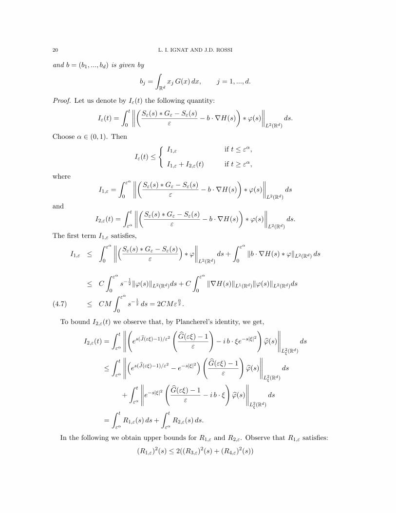
20 L. I. IGNAT AND J.D. ROSSI
and b = (b1, ..., bd) is given by
bj =∫
Rd
xj G(x) dx, j = 1, ..., d.
Proof. Let us denote by Iε(t) the following quantity:
Iε(t) =∫ t
0
∥∥∥∥(Sε(s) ∗Gε − Sε(s)ε
− b · ∇H(s))∗ ϕ(s)
∥∥∥∥L2(Rd)
ds.
Choose α ∈ (0, 1). Then
Iε(t) ≤
{I1,ε if t ≤ εα,
I1,ε + I2,ε(t) if t ≥ εα,
where
I1,ε =∫ εα
0
∥∥∥∥(Sε(s) ∗Gε − Sε(s)ε
− b · ∇H(s))∗ ϕ(s)
∥∥∥∥L2(Rd)
ds
and
I2,ε(t) =∫ t
εα
∥∥∥∥(Sε(s) ∗Gε − Sε(s)ε
− b · ∇H(s))∗ ϕ(s)
∥∥∥∥L2(Rd)
ds.
The first term I1,ε satisfies,
I1,ε ≤∫ εα
0
∥∥∥∥(Sε(s) ∗Gε − Sε(s)ε
)∗ ϕ
∥∥∥∥L2(Rd)
ds +∫ εα
0‖b · ∇H(s) ∗ ϕ‖L2(Rd) ds
≤ C
∫ εα
0s−
12 ‖ϕ(s)‖L2(Rd)ds + C
∫ εα
0‖∇H(s)‖L1(Rd)‖ϕ(s)‖L2(Rd)ds
≤ CM
∫ εα
0s−
12 ds = 2CMε
α2 .(4.7)
To bound I2,ε(t) we observe that, by Plancherel’s identity, we get,
I2,ε(t) =∫ t
εα
∥∥∥∥∥(
es(J(εξ)−1)/ε2
(G(εξ)− 1
ε
)− i b · ξe−s|ξ|2
)ϕ(s)
∥∥∥∥∥L2
ξ(Rd)
ds
≤∫ t
εα
∥∥∥∥∥(es(J(εξ)−1)/ε2 − e−s|ξ|2)(G(εξ)− 1
ε
)ϕ(s)
∥∥∥∥∥L2
ξ(Rd)
ds
+∫ t
εα
∥∥∥∥∥e−s|ξ|2(
G(εξ)− 1ε
− i b · ξ
)ϕ(s)
∥∥∥∥∥L2
ξ(Rd)
ds
=∫ t
εα
R1,ε(s) ds +∫ t
εα
R2,ε(s) ds.
In the following we obtain upper bounds for R1,ε and R2,ε. Observe that R1,ε satisfies:
(R1,ε)2(s) ≤ 2((R3,ε)2(s) + (R4,ε)2(s))

A NONLOCAL CONVECTION-DIFFUSION EQUATION 21
where
(R3,ε)2(s) =∫|ξ|≤R/ε
(es(J(εξ)−1)/ε2 − e−s|ξ|2
)2∣∣∣∣∣G(εξ)− 1
ε
∣∣∣∣∣2
|ϕ(s, ξ)|2dξ
and
(R4,ε)2(s) =∫|ξ|≥R/ε
(es(J(εξ)−1)/ε2 − e−s|ξ|2
)2∣∣∣∣∣G(εξ)− 1
ε
∣∣∣∣∣2
|ϕ(s, ξ)|2dξ.
With respect to R3,ε we proceed as in the proof of Lemma 4.2 by choosing δ and R as in (2.6)and (2.7). Using estimate (4.4) and the fact that |G(ξ)−1| ≤ C|ξ| and |J(ξ)−1+ ξ2| ≤ C|ξ|3for every ξ ∈ Rd we obtain:
(R3,ε)2(s) ≤ C
∫|ξ|≤R/ε
e−s|ξ|2s2
∣∣∣∣∣ J(εξ)− 1 + ξ2ε2
ε2
∣∣∣∣∣2
|ξ|2|ϕ(s, ξ)|2dξ
≤ C
∫|ξ|≤R/ε
e−s|ξ|2s2
[(εξ)3
ε2
]2
|ξ|2|ϕ(s, ξ)|2dξ
= C
∫|ξ|≤R/ε
e−s|ξ|2s2ε2|ξ|8|ϕ(s, ξ)|2dξ ≤ ε2s−2
∫Rd
e−s|ξ|2s4|ξ|8|ϕ(s, ξ)|2dξ
≤ Cε2−2α
∫Rd
|ϕ(s, ξ)|2dξ ≤ Cε2−2αM2.
In the case of R4,ε, we use that |G(ξ)| ≤ 1 and we proceed as in the proof of (4.3):
(R4,ε)2(s) ≤∫|ξ|≥R/ε
(e−sδε2 + e−
sR2
ε2 )2ε−2|ϕ(s, ξ)|2dξ
≤ (e−δ
ε2−α + e−R2
ε2−α )2ε−2
∫|ξ|≥R/ε
|ϕ(s, ξ)|2dξ
≤ M2(e−δ
ε2−α + e−R2
ε2−α )2ε−2
≤ CM2ε2−2α
for sufficiently small ε.Then
(4.8)∫ t
εα
R1,ε(s)ds ≤ CTMε1−α.
The second term can be estimated in a similar way, using that |G(ξ)− 1− ib · ξ| ≤ C|ξ|2 forevery ξ ∈ Rd, we get
(R2,ε)2(s) ≤∫
Rd
e−2s|ξ|2∣∣∣∣∣G(εξ)− 1− i b · ξε
ε
∣∣∣∣∣2
|ϕ(s, ξ)|2dξ
≤ C
∫Rd
e−2s|ξ|2[(ξε)2
ε
]2
|ϕ(s, ξ)|2dξ = C
∫Rd
e−2s|ξ|2ε2|ξ|4|ϕ(s, ξ)|2dξ
= Cε2s−2
∫Rd
e−2s|ξ|2s2|ξ|4|ϕ(s, ξ)|2dξ ≤ Cε2(1−α)
∫Rd
|ϕ(s, ξ)|2dξ
≤ CM2ε2(1−α),
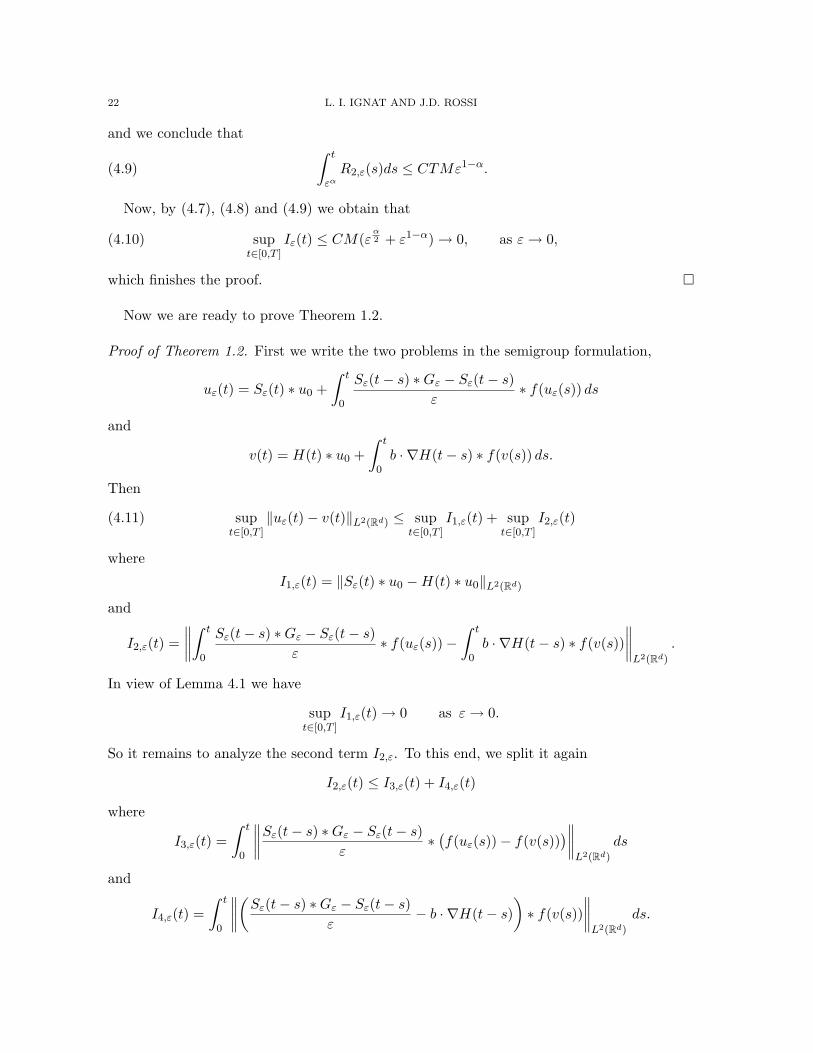
22 L. I. IGNAT AND J.D. ROSSI
and we conclude that
(4.9)∫ t
εα
R2,ε(s)ds ≤ CTMε1−α.
Now, by (4.7), (4.8) and (4.9) we obtain that
(4.10) supt∈[0,T ]
Iε(t) ≤ CM(εα2 + ε1−α) → 0, as ε → 0,
which finishes the proof. �
Now we are ready to prove Theorem 1.2.
Proof of Theorem 1.2. First we write the two problems in the semigroup formulation,
uε(t) = Sε(t) ∗ u0 +∫ t
0
Sε(t− s) ∗Gε − Sε(t− s)ε
∗ f(uε(s)) ds
and
v(t) = H(t) ∗ u0 +∫ t
0b · ∇H(t− s) ∗ f(v(s)) ds.
Then
(4.11) supt∈[0,T ]
‖uε(t)− v(t)‖L2(Rd) ≤ supt∈[0,T ]
I1,ε(t) + supt∈[0,T ]
I2,ε(t)
where
I1,ε(t) = ‖Sε(t) ∗ u0 −H(t) ∗ u0‖L2(Rd)
and
I2,ε(t) =∥∥∥∥∫ t
0
Sε(t− s) ∗Gε − Sε(t− s)ε
∗ f(uε(s))−∫ t
0b · ∇H(t− s) ∗ f(v(s))
∥∥∥∥L2(Rd)
.
In view of Lemma 4.1 we have
supt∈[0,T ]
I1,ε(t) → 0 as ε → 0.
So it remains to analyze the second term I2,ε. To this end, we split it again
I2,ε(t) ≤ I3,ε(t) + I4,ε(t)
where
I3,ε(t) =∫ t
0
∥∥∥∥Sε(t− s) ∗Gε − Sε(t− s)ε
∗(f(uε(s))− f(v(s))
)∥∥∥∥L2(Rd)
ds
and
I4,ε(t) =∫ t
0
∥∥∥∥(Sε(t− s) ∗Gε − Sε(t− s)ε
− b · ∇H(t− s))∗ f(v(s))
∥∥∥∥L2(Rd)
ds.

A NONLOCAL CONVECTION-DIFFUSION EQUATION 23
Using Young’s inequality and that from our hypotheses we have an uniform bound for uε
and u in terms of ‖u0‖L1(Rd), ‖u0‖L∞(Rd) we obtain
I3,ε(t) ≤∫ t
0
‖f(uε(s))− f(v(s))‖L2(Rd)
|t− s|12
ds
≤ ‖f(uε)− f(v)‖L∞((0,T ); L2(Rd))
∫ t
0
ds
|t− s|12
(4.12)
≤ 2T 1/2‖uε − v‖L∞((0,T ); L2(Rd))C(‖u0‖L1(Rd), ‖u0‖L∞(Rd)).
By Lemma 4.3 we obtain, choosing α = 2/3 in (4.10), that
(4.13) supt∈[0,T ]
I4,ε ≤ Cε13 ‖f(v)‖L∞((0,T ); L2(Rd)) ≤ Cε
13 C(‖u0‖L1(Rd), ‖u0‖L∞(Rd)).
Using (4.11), (4.12) and (4.13) we get:
‖uε − v‖L∞((0,T ); L2(Rd)) ≤ ‖I1,ε‖L∞((0,T ); L2(Rd))
+T12 C(‖u0‖L1(R), ‖u0‖L∞(R))‖uε − v‖L∞((0,T ); L2(Rd)).
Choosing T = T0 sufficiently small, depending on ‖u0‖L1(R) and ‖u0‖L∞(R) we get
‖uε − v‖L∞((0,T ); L2(Rd)) ≤ ‖I1,ε‖L∞((0,T ); L2(Rd)) → 0,
as ε → 0.Using the same argument in any interval [τ, τ + T0], the stability of the solutions of the
equation (1.3) in L2(Rd)-norm and that for any time τ > 0 it holds that
‖uε(τ)‖L1(Rd) + ‖uε(τ)‖L∞(Rd) ≤ ‖u0‖L1(Rd) + ‖u0‖L∞(Rd),
we obtainlimε→0
supt∈[0,T ]
‖uε − v‖L2(Rd) = 0,
as we wanted to prove. �
5. Long time behaviour of the solutions
The aim of this section is to obtain the first term in the asymptotic expansion of thesolution u to (1.1). The main ingredient for our proofs is the following lemma inspired in theFourier splitting method introduced by Schonbek, see [17], [18] and [19].
Lemma 5.1. Let R and δ be such that the function J satisfies:
(5.1) J(ξ) ≤ 1− |ξ|2
2, |ξ| ≤ R
and
(5.2) J(ξ) ≤ 1− δ, |ξ| ≥ R.
Let us assume that the function u : [0,∞) × Rd → R satisfies the following differentialinequality:
(5.3)d
dt
∫Rd
|u(t, x)|2 dx ≤ c
∫Rd
(J ∗ u− u)(t, x)u(t, x) dx,

24 L. I. IGNAT AND J.D. ROSSI
for any t > 0. Then for any 1 ≤ r < ∞ there exists a constant a = rd/cδ such that
(5.4)∫
Rd
|u(at, x)|2dx ≤‖u(0)‖2
L2(Rd)
(t + 1)rd+
rdω0(2δ)d2
(t + 1)rd
∫ t
0(s + 1)rd− d
2−1‖u(as)‖2
L1(Rd)ds
holds for all positive time t where ω0 is the volume of the unit ball in Rd. In particular
(5.5) ‖u(at)‖L2(Rd) ≤‖u(0)‖L2(Rd)
(t + 1)rd2
+(2ω0)
12 (2δ)
d4
(t + 1)d4
‖u‖L∞([0,∞); L1(Rd)).
Remark 5.1. Condition (5.1) can be replaced by J(ξ) ≤ 1 − A|ξ|2 for |ξ| ≤ R but omittingthe constant A in the proof we simplify some formulas.
Remark 5.2. The differential inequality (5.3) can be written in the following form:
d
dt
∫Rd
|u(t, x)|2 dx ≤ − c
2
∫Rd
∫Rd
J(x− y)(u(t, x)− u(t, y))2 dx dy.
This is the nonlocal version of the energy method used in [12]. However, in our case, exactlythe same inequalities used in [12] could not be applied.
Proof. Let R and δ be as in (5.1) and (5.2). We set a = rd/cδ and consider the following set:
A(t) =
{ξ ∈ Rd : |ξ| ≤ M(t) =
(2rd
c(t + a)
)1/2}
.
Inequality (5.3) gives us:
(5.6)d
dt
∫Rd
|u(t, x)|2dx ≤ c
∫Rd
(J(ξ)− 1)|u(ξ)|2dξ ≤ c
∫A(t)c
(J(ξ)− 1)|u(ξ)|2dξ.
Using the hypotheses (5.1) and (5.2) on the function J the following inequality holds for allξ ∈ A(t)c:
(5.7) c(J(ξ)− 1) ≤ − rd
t + a, for every ξ ∈ A(t)c,
since for any |ξ| ≥ R
c(J(ξ)− 1) ≤ −cδ = −rd
a≤ − rd
t + a
and
c(J(ξ)− 1) ≤ −c|ξ|2
2≤ − c
22rd
c(t + a)= − rd
t + a
for all ξ ∈ A(t)c with |ξ| ≤ R.

A NONLOCAL CONVECTION-DIFFUSION EQUATION 25
Introducing (5.7) in (5.6) we obtaind
dt
∫Rd
|u(t, x)|2dx ≤ − rd
t + a
∫A(t)c
|u(t, ξ)|2dξ
≤ − rd
t + a
∫Rd
|u(t, ξ)|2dξ +rd
t + a
∫|ξ|≤M(t)
|u(t, ξ)|2dξ
≤ − rd
t + a
∫Rd
|u(t, x)|2dx +rd
t + aM(t)dω0‖u(t)‖2
L∞(Rd)
≤ − rd
t + a
∫Rd
|u(t, x)|2dx +rd
t + a
[2rd
c(t + a)
] d2
ω0‖u(t)‖2L1(Rd)).
This implies thatd
dt
[(t + a)rd
∫Rd
|u(t, x)|2dx]
= (t + a)rd
[d
dt
∫Rd
|u(t, x)|2dx
]+ rd(t + a)rd−1
∫Rd
|u(t, x)|2dx
≤ (t + a)rd− d2−1rd
(2rd
c
) d2
ω0‖u(t)‖2L1(Rd).
Integrating on the time variable the last inequality we obtain:
(t+a)rd
∫Rd
|u(t, x)|2dx−ard
∫Rd
|u(0, x)|2dx ≤ rdω0
(2rd
c
) d2∫ t
0(s+a)rd− d
2−1‖u(s)‖2
L1(Rd)ds
and hence∫Rd
|u(t, x)|2 dx ≤ ard
(t + a)rd
∫Rd
|u(0, x)|2 dx
+rdω0
(t + a)rd
(2rd
c
) d2∫ t
0(s + a)rd− d
2−1‖u(s)‖2
L1(Rd) ds.
Replacing t by ta we get:∫Rd
|u(at, x)|2 dx ≤‖u(0)‖2
L2(Rd)
(t + 1)rd+
rdω0
(t + 1)rdard
(2rd
c
) d2∫ at
0(s + a)rd− d
2−1‖u(s)‖2
L1(Rd) ds
=‖u(0)‖2
L2(Rd)
(t + 1)rd+
rdω0
(t + 1)rd
(2rd
ca
) d2∫ t
0(s + 1)rd− d
2−1‖u(as)‖2
L1(Rd) ds
=‖u(0)‖2
L2(Rd)
(t + 1)rd+
rdω0(2δ)d2
(t + 1)rd
∫ t
0(s + 1)rd− d
2−1‖u(as)‖2
L1(Rd) ds
which proves (5.4).Estimate (5.5) is obtained as follows:∫
Rd
|u(at, x)|2dx ≤‖u(0)‖2
L2(Rd)
(t + 1)rd+
rdω0(2δ)d2
(t + 1)rd‖u‖2
L∞([0,∞); L1(Rd))
∫ t
0(s + 1)rd− d
2−1ds
≤‖u(0)‖2
L2(Rd)
(t + 1)rd+
2ω0(2δ)d2
(t + 1)d2
‖u‖2L∞([0,∞); L1(Rd)).

26 L. I. IGNAT AND J.D. ROSSI
This ends the proof. �
Lemma 5.2. Let 2 ≤ p < ∞. For any function u : Rd 7→ Rd, I(u) defined by
I(u) =∫
Rd
(J ∗ u− u)(x)|u(x)|p−1 sgn(u(x)) dx
satisfies
I(u) ≤ 4(p− 1)p2
∫Rd
(J ∗ |u|p/2 − |u|p/2)(x)|u(x)|p/2 dx
= −2(p− 1)p2
∫Rd
∫Rd
J(x− y)(|u(y)|p/2 − |u(x)|p/2)2 dx dy.
Remark 5.3. This result is a nonlocal counterpart of the well known identity∫Rd
∆u |u|p−1 sgn(u) dx = −4(p− 1)p2
∫Rd
|∇(|u|p/2)|2 dx.
Proof. Using the symmetry of J , I(u) can be written in the following manner,
I(u) =∫
Rd
∫Rd
J(x− y)(u(y)− u(x))|u(x)|p−1 sgn(u(x)) dx dy
=∫
Rd
∫Rd
J(x− y)(u(x)− u(y))|u(y)|p−1 sgn(u(y)) dx dy.
Thus
I(u) = −12
∫Rd
∫Rd
J(x− y)(u(x)− u(y))(|u(x)|p−1 sgn(u(x))− |u(y)|p−1 sgn(u(y))
)dx dy.
Using the following inequality,
||α|p/2 − |β|p/2|2 ≤ p2
4(p− 1)(α− β)(|α|p−1 sgn(α)− |β|p−1 sgn(β))
which holds for all real numbers α and β and for every 2 ≤ p < ∞, we obtain that I(u) canbe bounded from above as follows:
I(u) ≤ −4(p− 1)2p2
∫Rd
∫Rd
J(x− y)(|u(y)|p/2 − |u(x)|p/2)2 dx dy
= −4(p− 1)2p2
∫Rd
∫Rd
J(x− y)(|u(y)|p − 2|u(y)|p/2|u(x)|p/2 + |u(x)|p) dx dy
=4(p− 1)
p2
∫Rd
(J ∗ |u|p/2 − |u|p/2)(x)|u(x)|p/2 dx.
The proof is finished. �
Now we are ready to proceed with the proof of Theorem 1.4.

A NONLOCAL CONVECTION-DIFFUSION EQUATION 27
Proof of Theorem 1.4. Let u be the solution to the nonlocal convection-diffusion problem.Then, by the same arguments that we used to control the L1(Rd)-norm, we obtain the fol-lowing:
d
dt
∫Rd
|u(t, x)|pdx = p
∫Rd
(J ∗ u− u)(t, x)|u(t, x)|p−1 sgn(u(t, x)) dx
+∫
Rd
(G ∗ f(u)− f(u))(t, x)|u(t, x)|p−1 sgn(u(t, x)) dx
≤ p
∫Rd
(J ∗ u− u)(t, x)|u(t, x)|p−1 sgn(u(t, x)) dx.
Using Lemma 5.2 we get that the Lp(Rd)-norm of the solution u satisfies the following differ-ential inequality:
(5.8)d
dt
∫Rd
|u(t, x)|p dx ≤ 4(p− 1)p
∫Rd
(J ∗ |u|p/2 − |u|p/2)(x)|u(x)|p/2 dx.
First, let us consider p = 2. Then
d
dt
∫Rd
|u(t, x)|2 dx ≤ 2∫
Rd
(J ∗ |u| − |u|)(t, x)|u(t, x)| dx.
Applying Lemma 5.1 with |u|, c = 2, r = 1 and using that ‖u‖L∞([0,∞); L1(Rd)) ≤ ‖u0‖L1(Rd)
we obtain
‖u(td/2δ)‖L2(R) ≤‖u0‖L2(Rd)
(t + 1)d2
+(2ω0)
12 (2δ)
d4
(t + 1)d4
‖u‖L∞([0,∞); L1(Rd))
≤‖u0‖L2(Rd)
(t + 1)d2
+(2ω0)
12 (2δ)
d4
(t + 1)d4
‖u0‖L1(Rd))
≤C(J, ‖u0‖L1(Rd), ‖u0‖L∞(Rd))
(t + 1)d4
,
which proves (1.6) in the case p = 2. Using that the L1(Rd)-norm of the solutions to (1.1),does not increase, ‖u(t)‖L1(Rd) ≤ ‖u0‖L1(Rd), by Holder’s inequality we obtain the desireddecay rate (1.6) in any Lp(Rd)-norm with p ∈ [1, 2].
In the following, using an inductive argument, we will prove the result for any r = 2m,with m ≥ 1 an integer. By Holder’s inequality this will give us the Lp(Rd)-norm decay forany 2 < p < ∞.
Let us choose r = 2m with m ≥ 1 and assume that the following
‖u(t)‖Lr(Rd) ≤ C〈t〉−d2(1− 1
r)
holds for some positive constant C = C(J, ‖u0‖L1(Rd), ‖u0‖L∞(Rd)) and for every positive timet. We want to show an analogous estimate for p = 2r = 2m+1.
We use (5.8) with p = 2r to obtain the following differential inequality:
d
dt
∫Rd
|u(t, x)|2rdx ≤ 4(2r − 1)2r
∫Rd
(J ∗ |u|r − |u|r)(t, x)|u(t, x)|rdx.

28 L. I. IGNAT AND J.D. ROSSI
Applying Lemma (5.1) with |u|r, c(r) = 2(2r − 1)/r and a = rd/c(r)δ we get:∫Rd
|u(at)|2r ≤‖ur
0‖2L2(Rd)
(t + 1)rd+
dω0(2δ)d2
(t + 1)rd
∫ t
0(s + 1)rd− d
2−1‖ur(as)‖2
L1(Rd)ds
≤‖u0‖2r
L2r(Rd)
(t + 1)rd+
C(J)(t + 1)rd
∫ t
0(s + 1)rd− d
2−1‖u(as)‖2r
Lr(Rd)ds
≤C(J, ‖u0‖L1(Rd), ‖u0‖L∞(Rd))
(t + 1)d×(
1 +∫ t
0(s + 1)rd− d
2−1(s + 1)−dr(1− 1
r)ds
)≤ C
(t + 1)dr(1 + (t + 1)
d2 ) ≤ C(t + 1)
d2−dr
and then‖u(at)‖L2r(Rd) ≤ C(J, ‖u0‖L1(Rd), ‖u0‖L∞(Rd))(t + 1)−
d2(1− 1
2r),
which finishes the proof. �
Let us close this section with a remark concerning the applicability of energy methods tostudy nonlocal problems.
Remark 5.4. If we want to use energy estimates to get decay rates (for example in L2(Rd)),we arrive easily to
d
dt
∫Rd
|w(t, x)|2 dx = −12
∫Rd
∫Rd
J(x− y)(w(t, x)− w(t, y))2 dx dy
when we deal with a solution of the linear equation wt = J ∗ w − w and to
d
dt
∫Rd
|u(t, x)|2 dx ≤ −12
∫Rd
∫Rd
J(x− y)(u(t, x)− u(t, y))2 dx dy
when we consider the complete convection-diffusion problem. However, we can not go furthersince an inequality of the form(∫
Rd
|u(x)|p dx
) 2p
≤ C
∫Rd
∫Rd
J(x− y)(u(x)− u(y))2 dx dy
is not available for p > 2.
6. Weakly nonlinear behaviour
In this section we find the leading order term in the asymptotic expansion of the solutionto (1.1). We use ideas from [12] showing that the nonlinear term decays faster than the linearpart.
We recall a previous result of [15] that extends to nonlocal diffusion problems the result of[11] in the case of the heat equation.
Lemma 6.1. Let J ∈ S(Rd) such that
J(ξ)− (1− |ξ|2) ∼ B|ξ|3, ξ ∼ 0,

A NONLOCAL CONVECTION-DIFFUSION EQUATION 29
for some constant B. For every p ∈ [2,∞), there exists some positive constant C = C(p, J)such that
(6.1) ‖S(t) ∗ ϕ−MH(t)‖Lp(Rd) ≤ Ce−t‖ϕ‖Lp(Rd) + C‖ϕ‖L1(Rd,|x|)〈t〉− d
2(1− 1
p)− 1
2 , t > 0,
for every ϕ ∈ L1(Rd, 1 + |x|) with M =∫
R ϕ(x) dx, where
H(t) =e−
x2
4t
(2πt)d2
,
is the gaussian.
Remark 6.1. We can consider a condition like J(ξ) − (1 − A|ξ|2) ∼ B|ξ|3 for ξ ∼ 0 andobtain as profile a modified Gaussian HA(t) = H(At), but we omit the tedious details.
Remark 6.2. The case p ∈ [1, 2) is more subtle. The analysis performed in the previoussections to handle the case p = 1 can be also extended to cover this case when the dimensiond verifies 1 ≤ d ≤ 3. Indeed in this case, if J satisfies J(ξ) ∼ 1− A|ξ|s, ξ ∼ 0, then s has tobe grater than [d/2] + 1 and s = 2 to obtain the Gaussian profile.
Proof. We write S(t) = e−tδ0 + Kt. Then it is sufficient to prove that
‖Kt ∗ ϕ−MKt‖Lp(Rd) ≤ C‖ϕ‖L1(Rd,|x|)〈t〉− d
2(1− 1
p)− 1
2
andt
d2(1− 1
p)‖Kt −H(t)‖Lp(Rd) ≤ C〈t〉−
12 .
The first estimate follows by Lemma 2.3. The second one uses the hypotheses on J . Adetailed proof can be found in [15]. �
Now we are ready to prove that the same expansion holds for solutions to the completeproblem (1.1) when q > (d + 1)/d.
Proof of Theorem 1.5. In view of (6.1) it is sufficient to prove that
t− d
2(1− 1
p)‖u(t)− S(t) ∗ u0‖Lp(Rd) ≤ C〈t〉−
d2(q−1)+ 1
2 .
Using the representation (3.1) we get that
‖u(t)− S(t) ∗ u0‖Lp(Rd) ≤∫ t
0‖[S(t− s) ∗G− S(t− s)] ∗ |u(s)|q−1u(s)‖Lp(Rd) ds.
We now estimate the right hand side term as follows: we will split it in two parts, one inwhich we integrate on (0, t/2) and another one where we integrate on (t/2, t). Concerning thesecond term, by Lemma 2.4, Theorem 1.4 we have,∫ t
t/2‖[S(t− s) ∗G− S(t− s)] ∗ |u(s)|q−1u(s)‖Lp(Rd)ds
≤ C(J,G)∫ t
t/2〈t− s〉−
12 ‖u(s)‖q
Lpq(Rd)ds
≤ C(J,G, ‖u0‖L1(Rd), ‖u0‖L∞(R))∫ t
t/2〈t− s〉−
12 〈s〉−
d2(q− 1
p)ds
≤ C〈t〉−d2(q− 1
p)+ 1
2 ≤ Ct− d
2(1− 1
p)〈t〉−
d2(q−1)+ 1
2 .

30 L. I. IGNAT AND J.D. ROSSI
To bound the first term we proceed as follows,∫ t/2
0‖[S(t− s) ∗G− S(t− s)] ∗ |u(s)|q−1u(s)‖Lp(Rd) ds
≤ C(p, J, G)∫ t/2
0〈t− s〉−
d2(1− 1
p)− 1
2 (‖|u(s)|q‖L1(Rd) + ‖|u(s)|q‖Lp(Rd)) ds
≤ C〈t〉−d2(1− 1
p)− 1
2
(∫ t/2
0‖u(s)‖q
Lq(Rd)ds +
∫ t/2
0‖u(s)‖q
Lpq(Rd)ds)
= C〈t〉−d2(1− 1
p)− 1
2 (I1(t) + I2(t)).
By Theorem 1.4, for the first integral, I1(t), we have the following estimate:
I1(t) ≤∫ t/2
0‖u(s)‖q
Lq(Rd)ds ≤ C(‖u0‖L1(Rd), ‖u0‖L∞(Rd))
∫ t/2
0〈s〉−
d2(q−1)ds,
and an explicit computation of the last integral shows that
〈t〉−12
∫ t/2
0〈s〉−
d2(q−1)ds ≤ C〈t〉−
d2(q−1)+ 1
2 .
Arguing in the same manner for I2 we get
〈t〉−12 I2(t) ≤ C(‖u0‖L1(Rd), ‖u0‖L∞(Rd))〈t〉−
12
∫ t/2
0〈s〉−
dq2
(1− 1pq
)ds
≤ C(‖u0‖L1(Rd), ‖u0‖L∞(Rd))〈t〉− d
2(q− 1
p)+ 1
2
≤ C(‖u0‖L1(Rd), ‖u0‖L∞(Rd))〈t〉−d2(q−1)+ 1
2 .
This ends the proof. �
Acknowledgements.
L. I. Ignat is partially supported by the grants MTM2005-00714 and PROFIT CIT-370200-2005-10 of the Spanish MEC, SIMUMAT of CAM and CEEX-M3-C3-12677 of the RomanianMEC.
J. D. Rossi is partially supported by SIMUMAT (Spain), UBA X066, CONICET andANPCyT PICT 05009 (Argentina).
References
[1] P. Bates and A. Chmaj, A discrete convolution model for phase transitions, Arch. Rat. Mech. Anal.,150, 281–305, (1999).
[2] P. Bates, P. Fife, X. Ren and X. Wang, Travelling waves in a convolution model for phase transitions,Arch. Rat. Mech. Anal., 138, 105–136, (1997).
[3] P. Brenner, V. Thomee and L.B. Wahlbin, Besov spaces and applications to difference methods forinitial value problems, Lecture Notes in Mathematics, Vol. 434, Springer-Verlag, Berlin, 1975.
[4] C. Carrillo and P. Fife, Spatial effects in discrete generation population models, J. Math. Biol., 50(2),161–188, (2005).
[5] E. Chasseigne, M. Chaves and J. D. Rossi, Asymptotic behavior for nonlocal diffusion equations, J.Math. Pures Appl., 86, 271–291, (2006).
[6] X. Chen, Existence, uniqueness and asymptotic stability of travelling waves in nonlocal evolutionequations, Adv. Differential Equations, 2, 125–160, (1997).

A NONLOCAL CONVECTION-DIFFUSION EQUATION 31
[7] C. Cortazar, M. Elgueta and J. D. Rossi, A non-local diffusion equation whose solutions develop afree boundary, Annales Henri Poincare, 6(2), 269–281, (2005).
[8] C. Cortazar, M. Elgueta, J. D. Rossi and N. Wolanski, Boundary fluxes for non-local diffusion, J.Differential Equations, 234, 360–390, (2007).
[9] , How to approximate the heat equation with Neumann boundary conditions by nonlocal diffu-sion problems, to appear in Arch. Rat. Mech. Anal.
[10] F. Da Lio, N. Forcadel and R. Monneau, Convergence of a non-local eikonal equation to anisotropicmean curvature motion. Application to dislocations dynamics, to appear in J. Eur. Math. Soc.
[11] J. Duoandikoetxea and E. Zuazua, Moments, masses de Dirac et decomposition de fonctions. (Mo-ments, Dirac deltas and expansion of functions), C. R. Acad. Sci. Paris Ser. I Math., 315(6), 693-698,(1992).
[12] M. Escobedo and E. Zuazua, Large time behavior for convection-diffusion equations in RN , J. Funct.Anal., 100(1), 119–161, (1991).
[13] P. Fife, Some nonclassical trends in parabolic and parabolic-like evolutions. Trends in nonlinear anal-ysis, 153–191, Springer, Berlin, 2003.
[14] P. Fife and X. Wang, A convolution model for interfacial motion: the generation and propagation ofinternal layers in higher space dimensions, Adv. Differential Equations, 3(1), 85–110, (1998).
[15] I.L. Ignat and J.D. Rossi, Refined asymptotic expansions for nonlocal diffusion equations, preprint.[16] T. W. Korner. Fourier analysis. Cambridge University Press, Cambridge, 1988.[17] M. Schonbek, Decay of solutions to parabolic conservation laws, Comm. Partial Differential Equations,
5(5), 449–473, (1980).[18] , Uniform decay rates for parabolic conservation laws, Nonlinear Anal., 10(9), 943–956, (1986).[19] , The Fourier splitting method, Advances in geometric analysis and continuum mechanics
(Stanford, CA, 1993), Int. Press, Cambridge, MA, 1995, 269–274.[20] X. Wang, Metastability and stability of patterns in a convolution model for phase transitions, J.
Differential Equations, 183, 434–461, (2002).[21] L. Zhang, Existence, uniqueness and exponential stability of traveling wave solutions of some inte-
gral differential equations arising from neuronal networks, J. Differential Equations, 197(1), 162–196,(2004).
L. I. IgnatDepartamento de Matematicas,U. Autonoma de Madrid,28049 Madrid, Spainand
Institute of Mathematics of the Romanian Academy,P.O.Box 1-764, RO-014700 Bucharest, Romania.
E-mail address: [email protected]
Web page: http://www.uam.es/liviu.ignat
J. D. RossiDepto. Matematica, FCEyN UBA (1428)Buenos Aires, Argentina.
E-mail address: [email protected]
Web page: http://mate.dm.uba.ar/∼jrossi