International Journal of Astronomy and Astrophysics, 2014, 4, 683-698 Published Online December 2014 in SciRes. http://www.scirp.org/journal/ijaa http://dx.doi.org/10.4236/ijaa.2014.44062

How to cite this paper: Tokis, J.N. (2014) A Solution of Kepler’s Equation. International Journal of Astronomy and Astro-physics, 4, 683-698. http://dx.doi.org/10.4236/ijaa.2014.44062

A Solution of Kepler’s Equation John N. Tokis Technological Educational Institute of Epirus, Ioannina, Greece Email: JohnTokis@ioa.teiep.gr Received 27 October 2014; revised 24 November 2014; accepted 22 December 2014

Academic Editor: Ran Zhou, Theoretical High Energy Physics Group, Fermi National Accelerator Laboratory, China

Copyright © 2014 by author and Scientific Research Publishing Inc. This work is licensed under the Creative Commons Attribution International License (CC BY). http://creativecommons.org/licenses/by/4.0/

Abstract The present study deals with a traditional physical problem: the solution of the Kepler’s equation for all conics (ellipse, hyperbola or parabola). Solution of the universal Kepler’s equation in closed form is obtained with the help of the two-dimensional Laplace technique, expressing the universal functions as a function of the universal anomaly and the time. Combining these new expressions of the universal functions and their identities, we establish one biquadratic equation for universal anomaly ( )χ for all conics; solving this new equation, we have a new exact solution of the pre- sent problem for the universal anomaly as a function of the time. The verifying of the universal Kepler’s equation and the traditional forms of Kepler’s equation from this new solution are dis-cussed. The plots of the elliptic, hyperbolic or parabolic Keplerian orbits are also given, using this new solution.

Keywords Keplerian Motion, Universal Kepler’s Equation, Universal Anomaly, Two-Dimensional Laplace Transforms

1. Introduction In the Keplerian problem, a body of mass 2m follows a conic orbit, for which the focus is identified to the center of attracting body (with mass 1m ). The Keplerian motion is described by the fundamental differential equation of the physical two-body problem:

2

2 3

ddt r

µ= −r r (1)

where r is the vector position of the moving body related to the attraction center and µ the gravitational pa-

J. N. Tokis

684

rameter defined by ( )1 2 0G m mµ = + > (where G the Newtonian gravitational constant) (see [1], Equation (6.2.3)).

The traditional form of Kepler’s equation, which can be obtained directly from Equation (1) (see [1], Section 6.3 and [2]), is normally written as:

For elliptic orbits ( )0 1ε≤ ≤ sin eE E Mε− = (2a)

for hyperbolic orbits ( )1 ε≤ sinh hE E Mε− = − (2b)

where ε is the eccentricity, E the eccentric anomaly and M the mean anomaly, which is defined as 1 2

3 2 , 0 1eM tµ ε= ≤ <a

(2c)

( )

1 2

3 2 , 1hM tµ ε= <−a

(2d)

( )1 2

1 23, 1

2pM t

q

µ ε= = (2e)

(see [2], Equation (11) and [3], Equations (4.35) and (4.51)). Remark that the time t is measured from peri-center and a is the semimajor axis, which is positive for ellipses, negative for hyperbolas, and infinite for pa-rabolas; also, q is the pericenter distance of the orbit. The case of 0ε = leads to a circular orbit and the sim-ple solution eE M= (cf., Equation (2a)), so that we will regard 0ε > hereafter in the present work.

Johannes Kepler announced the relevant laws of above equation early in 1609 and 1619 [4]. He has used physics as a guide in this discovery [5]. For four centuries, the Kepler’s problem is to solve the nonlinear Ke-pler’s Equation (2) for the eccentric anomaly.

Early analytical solution of Kepler’s equation was considered in a comprehensive study of Tisserand [6]. Re-cently, analytical works of the solution and use of Kepler’s equation have been proposed by various authors (see, e.g., [7]-[12]).

In virtually every decade from 1650 to the present, there have appeared papers devoted to the solution of this Kepler’s equation. Its exact analytical solution is unknown, and therefore, efficient procedures to solve it nu-merically have been well discussed in many standard text books of Celestial Mechanics and Astrodynamics as well as in a large number of papers. Colwell [13] contains extensive references to the Kepler problem in his book. During last two decades, studies were carried out by several investigators of the present problem [2] [14]-[18]. In these studies, they used numerical or approximations methods for solution of the Kepler’s equation. Hence, it appears that an analytical solution of the Kepler’s equation will be of great interest.

In the current study, an analytical investigation of the Kepler’s equation real roots in closed form is presented. In Section 2, we will establish the general form of Kepler’s equation and will clear up the useful identities of the universal functions. In Section 3, using the two-dimensional Laplace transform technique, we will present an analytical solution for the universal Kepler’s equation, obtaining the universal functions ( ), 0,1, 2,3nU n = as function of the universal anomaly ( )χ and the time ( )t . In Section 4, in the first step we will establish one new biquadratic equation for universal anomaly χ for all conics with the help of Newman’s equation (cf. Eq-uation (23)) and some identities of the new expressions of universal functions. Then, the solution ( )tχ χ= of the present problem has been obtained, solving this biquadratic equation for all conics.

Finally, discussion of the results, thus obtained, is presented in Section 5; the new solution of the problem will prove that verifies the traditional form of Kepler’s equations for elliptic, hyperbolic or parabolic orbits. The el-liptic, hyperbolic or parabolic Keplerian motion is easily plotted, using this new solution.

2. General Form of Kepler’s Equation In order to solve the Kepler’s Equation (2), we use here the generalized form of this equation with the universal functions and the universal anomaly instead of the eccentric anomaly (see [3], Section 4.5).

J. N. Tokis

685

Working for the Kepler’s Equation (2), we consider an object following a path of same eccentricity ε about the center of attracting body; the object is at time t in (vector) position ( )r t with (vector) velocity 0v . The time t is measured from the pericenter passage; so, when 0 0t = this object was at position 0r (with 0 0r=r ) of the pericenter with velocity 0v (with 0 0υ=v ) and eccentric anomaly 0 0E = . We emphasize that the vec-tors r and 0r originate at the center of attraction. Then, we introduce the universal anomaly χ , which is de-fined by Sundman transformation:

1 2d dt rµ χ= (3)

(see [3], Equation (4.71)) and related to the classical eccentric anomaly by

, 0E a aχ≡ > (4a)

, 0E a aχ≡ − < (4b)

, 0D aχ≡ = (4c)

where E is the eccentric anomaly angle of elliptic or hyperbolic orbit and D the parabolic eccentric anomaly of parabolic orbit with dimension 1 2L (see [9], Equation (18)). The α denotes the reciprocal of the semimajor axis a , namely

220

0

1 2 2ar r

υυµ µ

≡ ≡ − = −a

(5a,b,c)

Depending on the sign of α or the value of the eccentricity ε , the type of the orbit is determined such that: 0α > (or 1ε < ) for elliptic orbits; 0α < (or 1ε > ) for hyperbolic orbits and 0α = (or 1ε = ) for para-

bolic orbits. Note that the universal anomaly χ is a new independent variable with dimension 1 2L (see [3], Equation (4.70)).

From the initial condition 0 0E = and the known relations: 0 0cos 1E r aε = − , 0 0sinE aε σ= for elliptic orbits and 0 0cosh 1E r aε = − , 0 0sinhE aε σ= for hyperbolic orbits (see [3], Sections 4.3 and 4.4), we have also for the present problem

( ) 0 00 0 1 21 , 0q r ε σ

µ⋅

= = − ≡ =r v

a (6a,b)

where q stands for the pericenter distance of the orbit related to the parameter p with the relation

( ) ( )21 1p qε ε= − = +a (7)

Remark that the p is a non-negative parameter and the pericenter distance q may be positive or zero; both of them have dimensions of length (see [3], Section 4.1).

Now, using the universal functions defined by

( ) ( )( )

2

0; , 0,1, 2,3,

2 !

k n k

nk

U nn kα χ

χ α+∞

=

−= =

+∑ (8)

with their following useful properties:

( ) ( )10; ; d , 1, 2,3,n nU U n

χχ α χ α χ−= =∫ (9a)

( ) ( )2; ; , 0,1, 2,3,!

n

n nU U nnχχ α α χ α++ = = (9b)

( ) ( )1

;; , 1, 2,3,n

n

UU n

χ αχ α

χ −

∂= =

∂ (9c)

( ) ( )01

;;

UaU

χ αχ α

χ∂

= −∂

(9d)

(see [3], Equation (9.73)), the two forms of Kepler’s Equation (2) are incorporated in one universal equation

J. N. Tokis

686

( ) ( ) 1 21 3; ;qU U tχ α χ α µ+ = (10)

which is a standard form of the traditional Kepler’s Equations (2) with the epoch at pericenter passage (see [9], Equation (23) and [2], Equation (29)). The general formula (10) is valid for all values of α and ε ; in particu-lar, it is good for parabolic orbits where 1 0a = =a .

To find out the expression of many orbital quantities, e.g. the magnitude of the position vector ( )r t , we must solve the standard universal form (10) of the Kepler’s equation for the universal anomaly as function of the time, namely ( )tχ χ= .

3. Solution of the Universal Kepler’s Equation In order to obtain the analytical solution of the present problem, we shall solve first the universal Kepler’s equa-tion Equation (10), obtaining the universal functions nU , 0,1, 2,3n = as a function of the universal anomaly and the time. For this purpose, we will use the double Laplace transformation technique, which was analytically studied by Aghili and Salkhordeh-Moghaddam [19] and by Valkó and Abate [20].

The universal functions 2U : For this case, we introduce a new variable ( ), tω χ so that

( )2 ,U tω χ≡ (11a)

21

UU χωχ∂

= =∂

(11b)

3 20 0d dU U

χ χχ ω χ= =∫ ∫ (11c)

(see Equations (9)) and the universal Kepler’s Equation (10) becomes 1 2

0dq t

χχω ω χ µ+ =∫ (12a)

From the initial condition 0E = or 0χ = and Equation (9a), we have the corresponding initial conditions to the Equation (12a)

( ) ( )0, 0, 0xt tω ω= = (12b)

The application of double Laplace transform (with respect to χ and t ) to the Equations (12) gives the so-lution ( ),s ξΩ in transform domain as

( ) ( )1 2

2 2,

1s

qsµξ

ξΩ =

+ (13)

where s and ξ are the transform variables of χ and time t , respectively. For the solution of partial diffe-rential Equation (12a), we use the Appendix.

Now, the universal function 2U can be obtained by taking the inverse transform of Equation (13) (cf., Ap-pendix). So, we get

( ) 1 22 , AU t t

qω χ µ= = (14)

where we have abbreviated ( )1 2 1 2sin , 0A q q qχ≡ > (15)

with dimensions: [ ] 1 2A L= . The universal functions 3U : For this case, we will use a new variable ( ), tψ χ so that

( )3 ,U tψ χ≡ (16a)

32

UU χψ

χ∂

= =∂

(16b)

21

UU χχψχ

∂= =

∂ (16c)

J. N. Tokis

687

(see Equations (9c)) and the universal Kepler’s Equation (10) becomes 1 2q tχχψ ψ µ+ = (17a)

For 0E = or 0χ = and Equation (9a), we have the initial conditions to the Equation (17a)

( ) ( ) ( )0, 0, 0, 0t t tχ χχψ ψ ψ= = = (17b)

Similarly as in the case of 2U , using the double Laplace transform (with respect to χ and t ) for the Equa-tions (17), we obtained the solution ( ),s ξΨ in transform domain as

( ) ( )1 2

2 2,

1s

s qsµξ

ξΨ =

+ (18)

(cf., Appendix). Inverting ( ),s ξΨ we have the universal function 3U

( ) ( ) 1 23 , 1U t B tψ χ µ= = − (19)

where we have defined the non-dimensional function

( )1 2cos , 0B q qχ≡ > (20)

Then, substituting the results of Equation (14) and (19) into the relations 1 3U aU χ+ = and 0 2 1U aU+ = (cf., Equation (9b)), respectively, we can easily obtain the new universal functions 1U and 0U as

( ) 1 21 1U B tχ αµ= − − (21)

1 20 1 AU t

qαµ= − (22)

where A and B are given from Equations (15) and (20), respectively.

4. Analytical Solution of the Problem In order to obtain a solution for the universal anomaly ( )tχ χ= , we use the explicit expression for χ :

1 2tχ αµ σ= + (23)

where 1 2σ µ= ⋅r v . This relation was discovered by C. M. Newman and its χ does not involve any of the universal functions nU (see [3], Equation (4.86)). The σ can be also given by the known equation (see [3], Equation (4.83))

( ) 11 q Uσ α= − (24)

Substituting Equation (24) (with 1U given by (21)) into Equation (23), the following relation is obtained

( )( ) 1 2 1 21 1q q B t tχ α µ µ+ − − = (25)

To find out two more relations between χ , A and B , similar to Equation (25), we will use the basic rela-tion ( ) ( )2 1 2 2 1 2sin cos 1q qχ χ+ = and the definitions of A and B Equations (15) and (20), respectively. Thus, we can easily obtain the relation

2 2 1B A q+ = (26)

Further, we can find one more relation using the basic identity ( )21 2 01U U U= + (see [3], Equation (4.93));

indeed, with the help of Equations (14), (21) and (22), we obtain the relation

( )21 2 1 2 1 21 2A AB t t t

q qχ αµ µ αµ

− − = − (27)

The three Equations (25), (26) and (27) are a system of the three unknowns: χ , A and B . Solving this system, we get from two Equations (25) and (26) the following relations

J. N. Tokis

688

( ) ( )1 2 1 2 1 21 qB t t tµ µ χ αµε

− = − − (28a)

( )1 22 21 2 1 2

2

A t qt tq q

µµ χ αµε

= − −

(28b)

Finally, substituting Equations (28) into Equation (27), we obtain the following biquadratic equation for uni-versal anomaly χ

4 22 0 0z b z b+ + = (29)

where we have abbreviated 1 2z tχ αµ≡ − (30a)

( )2

2 32 1 2tb qqµε ε

≡ − +

(30b)

( )2 2

220 31 4t tb

q qµ µε ε

≡ − −

(30c)

with dimensions: [ ] 1 2z L= , [ ]2b L= and [ ] 20b L= .

The solution of the biquadratic Equation (29) gives the relation between the universal anomaly χ and the time t for all conics: ellipse, hyperbola or parabola. The solution of this equation can be obtained using the standard formula of the solution for biquadratic equation.

Solving the new biquadratic Equation (29), we get the solution of the present problem for the universal ano-maly χ at time 0t ≥ as shown below

( )1 2t tχ αµ ϕ= + (31)

where we have abbreviated

( ) ( ) ( )1 21 21 2 2 3 2 32 1 2 1t q t q t qϕ εµ ε ε µ ≡ + − − −

(32a)

particularly, for elliptic orbits ( )0 1ε< < we have

( ) ( )( )1 221 21 2 2 2 31 1 1t t qϕ ε ε εµ

≡ − − − + a (32b)

for hyperbolic orbits ( )1 ε<

( ) ( ) ( )( )1 221 21 2 2 3 21 1 1t t qϕ ε εµ ε

≡ − − − + − a (32c)

and for parabolic orbits ( )1ε =

( ) ( ) ( ) 1 21 21 2 2 32 1 1p t q t qϕ µ≡ + − (32d)

Remark that the discriminant of the biquadratic Equation (29) is ( )2 2 30 16 1 0q t qεµ∆ = + > , for 0q > .

Consequently, the solution (31) is real in the cases of hyperbolic and parabolic cases since the corresponding ( )tϕ , given from Equations (32c,d), are always real-valued. In the case of the elliptic Keplerian orbits, the Equ-

ation (31) is real only in the special case for which ( )tϕ , given from Equation (32b), becomes real, namely for the case

( )( )

21 2

3 2

4 or 2 11

et M

qµ ε

ε< < −

− (32e,f)

where eM is the mean anomaly defined by Equation (2c). The upper limit of this mean anomaly eM is de-

J. N. Tokis

689

fined from the relation (32f) for every completed trip of the orbiting body in its elliptic orbit about the center of the attracting body; this limit is useful for determination of each Keplerian ellipse (cf., the applications in the next section).

In the case of parabolic orbits where the limiting case →∞a (or 0α = ) and 1ε → corresponds to 0 2r q p= = and 1 2

0 0 0 0σ µ= ⋅ =r v , the equation (29) and its solution (31) are reduced to 4 2 24 4 0q t qχ χ µ+ − = (33a)

( ) ( ) ( )1 21 21 2 2 32 1 1p t q t qχ ϕ µ = = + −

(33b)

The Equation (31) is the solution of the present problem for all conics (ellipse, hyperbola or parabola) and expresses the relation between the universal anomaly χ and the time t.

Knowing the solution of the universal anomaly ( )tχ , we establish the exact expressions of the universal functions nU , n = 0, 1, 2, 3 as functions of the time t . Indeed, using Equation (31), the Equation (28) are ob-tained as functions of the time t :

1 21 2 2

31 1A qt tq q

εµ µε

= + −

(34a)

( ) ( )1 2 1 21 qB t t tµ µ ϕε

− = − (34b)

Then, the universal functions (19), (14), (21) and (22) are expressed as functions of the time t as show below

( )1 23

qU t tµ ϕε

= − (35a)

1 22

2 31 1qU tqε µ

ε

= + −

(35b)

( )11U tϕε

= (35c)

( )1 2

20 3

1 1 1 1U tqεε µ

ε

= − − +

(35d)

The magnitude of the position vector r of the orbiting body is

( ) ( ) ( )0 0 2 2; ; ;r r U U q Uχ α χ α ε χ α= + = + (36a,b)

(see [3], Equation (4.82) and [14], Equation (8)). Substituting into Equation (36b) the new expressions of 2U , given by Equation (35b), we obtain the time-dependent distance r of the orbiting body from the center of at-traction as

1 22

31r q tqε µ

= +

(37)

Furthermore, if we work in the orbital reference system with the origin at the attracting center (or focus), we chose the ( ),X Y plane to be the plane of motion with X -axis pointing toward pericenter and Y -axis in the direction for which the true anomaly ( )f is 90˚; in this way the Z -axis is parallel to the angular momentum. Then, if X and Y are the coordinates of a point ( ),P X Y on the conic orbit, we have cosX r f= and

r p Xε= − (38)

where p is the non-negative quantity given by Equation (7) (see [3], Equation (4.3)). Thus, the X and Y coordinates can be expressed as function of the time t , using Equations (38) and the identities: 2 2

0 1 1U aU+ = , ( )2

1 2 01U U U= + ; namely, we get

J. N. Tokis

690

( )2 ;X q U χ α= − (39a)

( ) ( )1 21 211 ;Y q Uε χ α= + (39b)

where 1U and 2U are given from Equations (35) (see [14], Equations (6)-(7)).

5. Discussion Using the standard form of the universal Kepler’s equation (10) with the epoch at pericenter passage, we have derived a new biquadratic equation (29) for universal anomaly χ as a function of the time t . This equation governs the motion of an orbiting body following a path with position vector ( )r t from the center of attracting body and with velocity vector ( )tv .

The new solution (31) of the present problem was obtained solving Equation (29) with initial-value conditions for the orbiting body at time 0t = passages from the pericenter, with minimum position vector 0r , velocity vector 0v and eccentric anomaly 0 0E = .

The solution (31) is a solution of the present problem. Indeed, the new expressions of the universal functions 3U , and 1U given by (35a,c) verify universal Kepler’s Equation (10). Moreover, the solution (31) is a solution

of the Equation (29), since it can be easily verified by substitution of (31) into (29). The solution (31) verifies also the traditional forms of Kepler’s Equation (2). Particularly, in the case of ellip-

tic orbits ( )0 1ε< < the solution (31) of the problem is reduced for the eccentric anomaly (cf. Equation (4a)) to the form

( )1 2e eE M tα χ ϕ= = + (40)

where eM is the mean anomaly given by Equation (2c) and

( ) ( ) ( ) ( )( )1 221 231 2 2 21 1 1 1e et t Mϕ α ϕ ε ε ε ε

≡ = − − − + − (41)

Note that ( ) 1e tϕ < and ( )1 22 1eM ε< − (cf. Equation (32f)) for 0 1ε< < .

Similarly, in the case of hyperbolic orbits ( )1 ε< the solution (31) of the problem is reduced, for the eccen-tric anomaly (cf. Equation (4b)), to

( ) ( )1 2h hE a M tχ ϕ= − = − + (42)

where hM is the mean anomaly given by Equation (2d) and

( ) ( ) ( ) ( ) ( )( )1 221 21 2 32 21 1 1 1h et t Mϕ α ϕ ε ε ε ε

≡ − = + − + − − (43)

Finally, in the case of parabolic orbits ( )1ε = the solution (33b) gives for the parabolic eccentric anomaly (cf. Equations (4c) and (2e)):

( ) ( ) ( )1 2

1 21 2 22 1 2 1 .p pD x t q Mϕ = = = + − (44)

From the other hand, the standard and hyperbolic trigonometric functions of Equations (2) are expressed as

( ) ( )1 2 1 21sin sin e t

E Uϕ

α χ αε

= = = (45a)

( ) ( ) ( )1 2 1 21sinh sinh h t

E Uϕ

α χ αε

= − = − = (45b)

where we have use Equation (35) and the relationship between the function U1 and the standard and hyperbolic trigonometric functions of Equations (2): ( )1 2 1 2

1 sinU α α χ−= and ( ) ( )1 2 1 21 sinhU α α χ− = − − for ellipse

J. N. Tokis

691

and hyperbola, respectively (see [3], Problem 4 - 21 and [9], Equation (24)). Now, we will prove that the Equations (40) and (42) represent the solutions of the traditional forms of Kep-

ler’s Equations (2). Indeed, it can be shown that the left-hand sides of Equations (2) are reduced to the right- hand sides, namely

( ) ( )sin e

e e e

tE E M t M

ϕε ϕ ε

ε− = + − = (46a)

( ) ( )sinh h

h h h

tE E M t M

ϕε ϕ ε

ε− = − + − = − (46b)

in accordance with the Equations (40), (42) and (45). It should be pointed out that our solutions for eccentric anomaly (cf., Equations (40) and (42)) are ready for

physical applications in the corresponding Keplerian orbits. In addition to above Keplerian orbits, the new solution (33b) of the present problem for the case of parabola

( 1ε = and 0α = ) verifies the traditional Barker’s equation for parabolic orbits 3 1 26 6q tχ χ µ+ = (47)

Remark that the parabolic Keplerian equation is called Barker’s equation (see [3], Equation (4.24)). Indeed, from the definition (8) for the universal functions we have ( )3

36 ;0Uχ χ= and ( )1 ;0Uχ χ= . Using the solu-tion (33b), these universal functions are expressed from Equations (35a,c), so that

( ) ( )3 1 26 6 , p pt q t tχ µ ϕ χ ϕ= − = (48a,b)

where ( )p tϕ is given from Equation (32d). Then, the left-hand side of Equations (47) is reduced to the right- hand side, namely

( ) ( )3 1 2 1 26 6 6 6 6p pq t q t q t tχ χ µ ϕ ϕ µ+ = − + = (49)

In order to study the Keplerian orbits with the help of the new solutions, we use also the cartesian coordinates x and y with the origin at the center of the ellipse or hyperbola. In this case the X and Y coordinates of the orbital ( ),X Y plane system given by Equations (39) are related to the system ( ),x y with the relations X x ε= − a and Y y= (see [3], Equation (4.4)); so, for the case 1ε ≠ , these new coordinates can be obtained

in the explicit forms x ζ ε= a (50a)

( ) ( )22 2 21 1y ε ζ ε = − − a (50b)

where we have defined the non-dimensional relation

( )1 2

231 1 1 t

qεζ ε µ

≡ − − +

(51)

in accordance to the Equations (39). Then, we introduce the non-dimensional coordinates

xεζ ≡a

(52a)

( )22

2 22 1 1y ζη ε

ε

≡ = − − a

(52b)

The new expressions (52) verify the following equations of ellipse ( )1ε < and hyperbola ( )1ε > , respec-tively:

2 2

2 2 11

ζ ηε ε

+ =−

(53a)

2 2

2 2 11

ζ ηε ε

− =−

(53b)

J. N. Tokis

692

where ζ is defined by Equation (51). Remark that the equations (53) are the non-dimensional forms of the el-lipse and hyperbola, respectively, in the cartesian system ( ),x y with the origin at the center of the ellipse or hyperbola (see [1], Equations (A.2.1) and (A.4.2)).

In the other hand, for the case of parabola ( )1ε = , the coordinates X and Y can be also obtained, from Equations (39), as following

( )1 22 32 1X q t qµ = − + (54a)

( )1 21 22 32 1 1Y q t qµ = + −

(54b)

Then, we have, from Equations (54),

( ) ( )2 14 22

Y q q X p p X= − = − (55a,b)

The last Equation (55) is the equation of parabola, which passes through its pericenter with coordinates ( )1 ,02

p

(see [3], Equation (3.22)). The non-dimensional form of Equation (55) is 2 4η ζ= (56)

with the non-dimensional coordinates

( )1 22 3 1 21 1, 2t qζ µ η ζ≡ + − ≡ (57a,b)

In addition to above results for the non-dimensional coordinates we have (for physical application) the cor-responding expressions:

For elliptic orbits ( )0 1ε< < the Equation (51) becomes

( )( )

1 2

231 1 1

1eMεζ ε

ε

≡ − − +

− (58a)

for hyperbolic orbits ( )1 ε< the Equation (51) becomes

( )( )

1 2

231 1 1

1hMεζ ε

ε

≡ + − +

− (58b)

for parabolic orbits ( )1ε = the Equation (57a) yields

( )1 221 2 1pMζ ≡ + − (58c)

where eM , hM and pM are the mean anomalies of ellipse, hyperbola and parabola, respectively (cf., Equa-tions (2c,d,e)). These mean anomalies can be varied from 0 to 2 πk , where k is an integer. Note that the non- dimensional coordinates of attractive center (or focus) F in the non-dimensional cartesian system ( ),ζ η is given by ( )2 ,0F ε for all Keplerian orbits (ellipse, hyperbola or parabola).

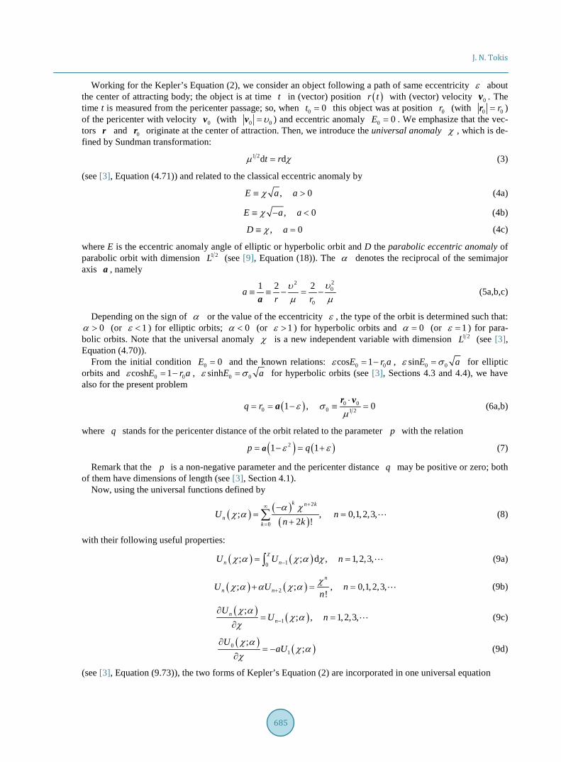
In order to get a physical insight into the new solution of the Kepler’s problem, we apply the above results for the system Earth-Moon. For this system the eccentricity of the Moon is 0.0549ε = and the upper limit for the mean anomaly can be obtained from relation (32f) as 1.94432eM < . So, varying the mean anomaly eM (with

1.944eM ≤ ) and using Equations (58a) and (52b), the elliptic Keplerian motion of the Moon about the Earth can be easily plotted in the non-dimensional cartesian system ( ),ζ η (Figure 1). Remark that the non-dimen- sional coordinates of the Earth are obtained as ( )0.003,0 .

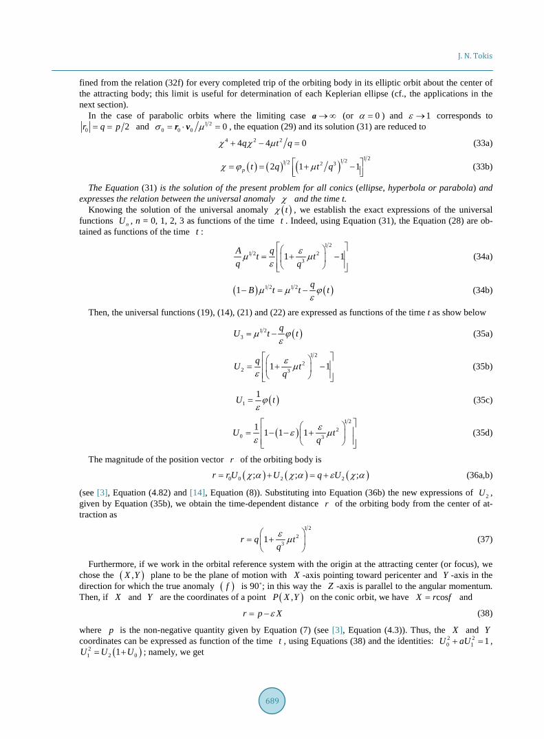
Note that the use of the upper limit of the mean anomaly, given from the relation ( )1 22 1eM ε< − (cf. rela-tion (32f)), is import for the plotting of all elliptic Keplerian orbits. To confirm that we give two more examples: (a) We consider an object following an elliptic orbit with eccentricity 0.5ε = about the center of attracting body; the upper limit of the mean anomaly, from relation (32f), is 1.4142eM < ; then, varying the mean ano-maly eM (with 1.414eM ≤ ) and using Equations (58a) and (52b), we plot the elliptic Keplerian orbit in the non-dimensional cartesian system ( ),ζ η (Figure 2). (b) We consider another object in an elliptic orbit with

J. N. Tokis

693

Figure 1. The elliptic orbit of the Moon ( )0.0549ε = about the Earth.

Figure 2. Two elliptic Keplerian orbits with eccentricities 0.5ε = and 0.97ε = .

eccentricity 0.97ε = about the center of another attracting body; the upper limit of the new mean anomaly, from relation (32f), is 0.3464eM < ; and, varying the mean anomaly eM (with 0.345eM ≤ ), we plot the el-liptic Keplerian orbit in the non-dimensional cartesian system ( ),ζ η (Figure 2).

Now, varying the mean anomaly hM (with 3.14hM ≤ for the present plot) and using equations (58b) and

J. N. Tokis

694

( ) ( )22 2 1 1η ε ζ ε = − − (cf., Equation (52b), we plot of the hyperbolic Keplerian motion of an orbiting body

with the eccentricity 1.3ε = about the attractive center ( )1.69,0F (Figure 3). Finally, varying the mean anomaly pM (with 2pM ≤ for the present plot) and using Equations (58c), and

(56), we plot of the parabolic Keplerian motion of an orbiting body with the eccentricity 1ε = about the attrac-tive center ( )1,0F (Figure 4).

6. Conclusions This work presents a solution to the well known Keplerian two body physical problem. From the investigation

Figure 3. The hyperbola of an orbiting body (with 1.3ε = ) about the attractive centre ( )1.69,0F .

Figure 4. The parabola of an orbiting body (with 1ε = ) about the attractive centre ( )1,0F .

J. N. Tokis

695

for this new solution, the main conclusions have been drawn as following: 1) An analytical solution for the universal Kepler’s equation has been determined, obtaining the universal

functions nU , n = 0, 1, 2, 3 as function of the universal anomaly ( )χ and the time ( )t with the help of the two-dimensional Laplace transform technique.

2) Using an explicit expression for the universal anomaly ( )χ without any of the nU functions (cf., Equa-tion (23)) and some identities of the new obtained universal functions, we developed a biquadratic equation for universal anomaly χ for all conics: ellipse, hyperbola or parabola.

3) The solution ( )tχ χ= of the present problem has been obtained, solving this biquadratic equation for all conics.

4) This new analytical solution for the universal anomaly has been discussed and proved that verifies the uni-versal Kepler’s equation (cf., Equation (10)), since the time depended universal functions U3 and U1 verify this equation. Then, the solutions for the eccentric anomaly (cf., Equations (40) and (42)) were also proved that ver-ify the traditional form of Kepler’s equations for elliptic or hyperbolic orbits. This new solution for the universal anomaly has also proved that verifies the traditional Barker’s equation for parabolic orbits [11]. The elliptic, hyperbolic or parabolic Keplerian motion is plotted, using this analytical solution.

5) To our knowledge, this work gives in closed form the actual analytical solution of the Kepler’s problem. The advantage of the new solution is simple and ready for physical applications in the elliptic, hyperbolic or parabolic Keplerian orbits.

References [1] Dandy, J.M.A. (2003) Fundamentals of Celestial Mechanics. 2nd Edition, Willmann-Bell, Virginia. [2] Fukushima, T. (1999) Fast Procedure Solving Universal Kepler’s Equation. Celestial Mechanics and Dynamical As-

tronomy, 75, 201-226. http://dx.doi.org/10.1023/A:1008368820433 [3] Battin, R.H. (1999) An Introduction to the Mathematics and Methods Astrodynamics. Revised Edition, AIAA Educa-

tion Series, New York. http://dx.doi.org/10.2514/4.861543 [4] Voelkel, J.R. (2001) The Composition of Kepler’s Astronomia Nova. Princeton University Press, New York.

http://press.princeton.edu/titles/7187.html [5] Bruce, S. (1987) Kepler’s Physical Astronomy. Springer-Verlag, New York. [6] Tisserand, F. (1894) Mécanique Céleste. Vol. 3. Gauthier-Villars, Paris. [7] Siewert, C.E. and Burniston, E.E. (1972) An Exact Analytical Solution of Kepler’s Equation. Celestial Mechanics, 6,

294-304. http://link.springer.com/article/10.1007/BF01231473#page-1 [8] Tokis, J.N. (1973) Effects of Tidal Dissipative Processes on Stellar Rotation. PhD Thesis, Victoria University of Man-

chester, Manchester. [9] Fernandes, S.daS. (2003) Universal Closed-form of Lagrangian Multipliers for Coast-Arcs of Optimum Space Trajec-

tories. Journal of the Brazilian Society of Mechanical Sciences and Engineering, 25, 1-9. http://dx.doi.org/10.1590/S1678-58782003000400004

[10] Condurache, D. and Martinusi, V. (2006) Vectorial Regularization and Temporal Means in Keplerian Motion. Journal of Nonlinear Mathematical Physics (World Scientific), 13, 420-440. http://dx.doi.org/10.2991/jnmp.2006.13.3.7

[11] Pathan, A. and Collyer, T. (2006) A Solution to a Cubic—Barker’s Equation for Parabolic Trajectories. Mathematical Gazette, 90, 398-403.

[12] Boubaker, K. (2010) Analytical Initial-Guess-Free Solution to Kepler’s Transcendental Equation Using Boubaker Poly- nomials Expansion Scheme BPES. Apeiron, 17, 1-12. http://redshift.vif.com/JournalFiles/V17NO1PDF/V17N1BOU.pdf

[13] Colwell, P. (1993) Solving Kepler’s Equation over Three Centuries. Willmann-Bell, Richmond. http://www.willbell.com/math/mc12.htm

[14] Floria, L. (1996) A Proof of Universality of Arc Length as Time Parameter in Kepler Problem. Extracta Mathematicae, 11, 315-324. http://dmle.cindoc.csic.es/pdf/EXTRACTAMATHEMATICAE_1996_11_02_09.pdf

[15] Fukushima, T. (1998) A Fast Procedure Solving Gauss Form of Kepler’s Equation. Celestial Mechanics and Dynami- cal Astronomy, 70, 115-130. http://link.springer.com/article/10.1023%2FA%3A1026479306748#page-1

[16] Sharaf, M.A. and Sharaf, A.A. (1998) Closest Approach in Universal Variables. Celestial Mechanics and Dynamical Astronomy, 69, 331-346. http://link.springer.com/article/10.1023%2FA%3A1008223105130#page-1

[17] Sharaf, M.A. and Sharaf, A.A. (2003) Homotopy Continuation Method of Arbitrary Order of Convergence for the

J. N. Tokis

696

Two-Body Universal Initial Value Problem. Celestial Mechanics and Dynamical Astronomy, 86, 351-362. http://link.springer.com/article/10.1023/A:1024544523868#page-1

[18] Jia, L. (2013) Approximate Kepler’s Elliptic Orbits with the Relativistic Effects. International Journal of Astronomy and Astrophysics, 3, 29-33. http://dx.doi.org/10.4236/ijaa.2013.31004

[19] Aghili, A. and Salkhordeh-Moghaddam, B. (2008) Laplace Transform Pairs of N-Dimensions and Second Order Linear Partial Differential Equations with Constant Coefficients. Annales Mathematicae et Informaticae, 35, 3-10. http://www.emis.de/journals/AMI/2008/ami2008-aghili-salkhordeh.pdf

[20] Valkó, P.P. and Abate, J. (2005) Numerical Inversion of 2-D Laplace Transforms Applied to Fractional Diffusion Equa- tion. Applied Numerical Mathematics, 53, 73-88. http://dx.doi.org/10.1016/j.apnum.2004.10.002

[21] Ditkin, V.A. and Prudnicov, A.P. (1962) Operational Calculus in Two Variables and Its Application. Pergamum Press, New York.

J. N. Tokis

697

Appendix Solution of partial differential equations using two-dimensional Laplace transforms

The general form of second-order linear partial differential equation in two variables is given as following

( )5 4 3 2 1 0 , , 0 , xx xy yy x yb f b f b f b f b f b f g x y x y+ + + + + = < < ∞ (A1)

where nb are constants and ( ),g x y is source function of x and y or constant. We use also the abbrevia-tions for the initial conditions

( ) ( ) ( ) ( )( ) ( ) ( ) ( ) ( )

1 2

3 4 0

,0 , 0, ,

,0 , 0, , 0,0 .y x

f x f x f y f y

f x f x f y f y f f

= =

= = = (A2)

and their one-dimensional Laplace transformations ( )1f s , ( )2f p , ( )3f s and ( )4f p , where “ s ” and “ p ” the transform variables of x and y , respectively (see [19] and [21] for details). Then, we get the relations for two-dimensional Laplace transforms

( ) ( ) ( )2 0 0, ; , , e , d dsx pyL f x y s p F s p f x y x y

∞ ∞ − −≡ = ∫ ∫ (A3a)

[ ] ( ) ( ) ( )22 2 4; , ,xxL f s p s F s p sf p f p= − − (A3b)

( ) ( ) ( )2 1 2 0; , ,xyL f s p spF s p sf s pf p f = − − − (A3c)

( ) ( ) ( )22 1 3; , ,yyL f s p p F s p pf s f s = − − (A3d)

[ ] ( ) ( )2 2; , ,xL f s p sF s p f p= − (A3e)

( ) ( )2 1; , ,yL f s p pF s p f s = − (A3f)

2 2

1; ,yL x s ps

= (A3g)

[ ]2 2

1; ,L x s ps p

= (A3h)

[ ]211; ,L s psp

= (A3i)

in accordance with the two-dimensional analysis formula, which can be written as one-dimensional analysis in the x direction followed by one-dimensional analysis in the y direction:

( ) ( )0 0

, e , d e dsx pyF s p f x y x y∞ ∞ − − = ∫ ∫ (A4)

Now, applying double Laplace transformation to both sides of Equation (A1) and using Equations (A3), we obtain the solution of Equation (A1) in the transform domain as

( )

( ) ( ) ( ) ( ) ( ) ( )( ) ( ) ( ) ( )

5 2 4 4 1 2 0

3 1 3 2 2 1 1

,1 ,,

.

F s p

g s p b sf p f p b sf s pf p fB s p

b pf s f s b f p b f s

= + + + + + −

+ + + +

(A5a)

with the abbreviation

( ) 2 25 4 3 2 1 0,B s p b s b sp b p b s b p b= + + + + + (A5b)

In order to invert this two-dimensional Laplace transform ( ),F s p , we follow the double inversion as a two-

J. N. Tokis

698

step process [20]. In the first step we invert, say, on the “ s ” transform variable

( ) ( )1, ,f x p L F s p−= (A6)

where we keep the second transform variable p as a constant. In the second step we invert on the “ p ” trans-form variable and obtain, finally,

( ) ( )1, ,f x y L f x p− = (A7)