1 Solution of a Non-Linear Equation

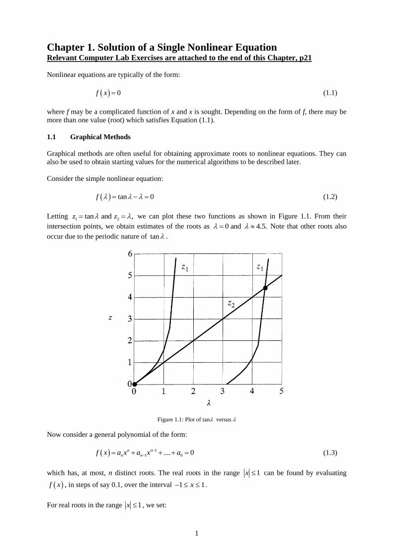
1

Chapter 1. Solution of a Single Nonlinear Equation Relevant Computer Lab Exercises are attached to the end of this Chapter, p21

Nonlinear equations are typically of the form:

0f x (1.1)

where f may be a complicated function of x and x is sought. Depending on the form of f, there may be

more than one value (root) which satisfies Equation (1.1).

1.1 Graphical Methods

Graphical methods are often useful for obtaining approximate roots to nonlinear equations. They can

also be used to obtain starting values for the numerical algorithms to be described later.

Consider the simple nonlinear equation:

tan 0f (1.2)

Letting 1 2tan and ,z z we can plot these two functions as shown in Figure 1.1. From their

intersection points, we obtain estimates of the roots as 0 and 4.5. Note that other roots also

occur due to the periodic nature of tan .

Figure 1.1: Plot of tan versus

Now consider a general polynomial of the form:

1

1 0.... 0n n

n nf x a x a x a

(1.3)

which has, at most, n distinct roots. The real roots in the range 1x can be found by evaluating

f x , in steps of say 0.1, over the interval 1 1x .

For real roots in the range 1x , we set:

2

1x z (1.4)

and rewrite (1.3) as

0)( 1

10

n

nn azazazf (1.5)

We then examine the behaviour of f z over the range 1 1z to find the roots in terms of z.

Once these are known, the roots in terms of x are found from (1.4).

To illustrate this technique, consider the polynomial equation:

3 24 10 2 6 0f x x x x (1.6)

Figure 1.2: Roots of cubic polynomial f x

Figure 1.3: Roots of cubic polynomial f z

3

For the roots in the range 1x we plot the function f x over the domain 1 1x at intervals of

0.2. From the plot of Figure 1.2, we see that roots occur at 0.75 and 0.8.x x For the roots in the

range 1x we plot the function

3 26 2 10 4 0f z z z z (1.7)

over the domain 1 1z at intervals of 0.2. From the plot of Figure 1.3 we see that a root occurs at

0.4.z This implies that a root occurs in the vicinity of 1 0.4 2.5.x

1.2 Bisection Algorithm

The bisection algorithm is one of the simplest methods for solving nonlinear equations. The method,

which is illustrated in Figure 1.4, is very robust and requires only that f x is continuous. To begin

the bisection algorithm, we need two values of lx and ux such that 0l uf x f x , which implies

that andl uf x f x must be of opposite sign. An improved estimate of the root is obtained by

computing the average of the end points lx and ux according to 1

1

2l ux x x

Figure 1.4: The bisection algorithm

If the product of 1f x and lf x is positive, then the new value for lx is set to 1x . Else, the new

value for ux is set to 1x . The whole process is then repeated in an iterative manner until the interval

u lx x becomes small. Thus the key idea behind the bisection method is to repeatedly halve the

interval in which the root must lie. All of the steps involved in the technique are shown in Algorithm

1.1.

Bisection Algorithm

In: End points l ux , x , tolerance , maximum number of iterations M.

Out: Solution x or error message.

f l = f ( x l )

loop i = 1 to M

1 u l

x

x = x + x - x 2

f = f x

if thenx l

l

l x

f f >0

x = x

f = f

else

ux = x

endif

4

if u 1x - x 2 ε then exit with root x

end loop

error: too many iterations.

Algorithm 1.1: The bisection algorithm

In the step which tests for convergence, is a small positive constant which determines the accuracy

of the computed solution. For typical floating point operations with a 32 bit word length, which gives

roughly 7 decimal digits of precision, is typically set somewhere in the range 10-5

to 10-6

. For double

precision arithmetic, where the machine accuracy is increased to approximately 15 decimal digits,

much smaller values can be employed. In most engineering applications, an accuracy of 10-6

is

sufficient.

Note that a variety of checks may be used to test for convergence. Each of these have particular

advantages and disadvantages, some of which will be discussed later in this Section. In the bisection

algorithm we insist that the interval which brackets the root is small so that 2 .u lx x Imposing

this condition guarantees that the best estimate for the root, which is the midpoint 2u ex x x ,

has an absolute error less than or equal to . The absolute sign is required in the test since we are only

interested in the magnitude of u lx x , and not its sign. Since we do not insist that u lx x , this

difference may in fact be negative and the algorithm will still work.

In all numerical methods for solving nonlinear equations, we also have to be careful of multiple roots

which, depending on the function, may be quite close together.

Each iteration of the bisection method halves the interval containing the root. Thus the number of

iterations required for convergence is given by the expression

22

u l

n

x x

(1.8)

or

2

10

10

10

log 2

1log 2

log 2

3.32log 2

u l

u l

u l

n x x

x x

x x

(1.9)

This implies that the number of iterations required for the bisection algorithm can always be estimated

beforehand.

To illustrate the bisection algorithm, consider the solution of the polynomial equation

2 2 3 1 3 0f x x x x x (1.10)

which has roots at 1 and 3.x x Let us start the iterations with the values 1 and 4l ux x

which bracket the positive root and set the convergence tolerance = 0.01. Substituting 3u lx x

and = 0.01, we predict from (1.9) that the algorithm will require precisely 8 iterations to isolate the

root. The iterations proceed as follows:

Input: 1, 4, 0.01l ux x

5

4l lf f x

Iteration 1:

2 2.5l u lx x x x

2.5 1.75xf f

1.75 4 7x lf f

0x lf f

2.5

1.75

l

l x

x x

f f

2 4 2.5 2 0.75u lx x

Iteration 2:

2 3.25l u lx x x x

3.25 1.0625xf f

1.0625 1.75 1.859375x lf f

0x lf f

3.25ux x

2 3.25 2.5 2 0.375u lx x

Iteration 3:

2 2.875l u lx x x x

2.875 0.484375xf f

0.484375 1.75 0.847656x lf f

0x lf f

2.875

0.484375

l

l x

x x

f f

2 3.25 2.875 2 0.1875u lx x

Iteration 4:

2 3.0625l u lx x x x

3.0625 0.253906xf f

0.253906 0.484375 0.122986x lf f

0x lf f

3.0625ux x

2 3.0625 2.875 2 0.09375u lx x

Iteration 5:

2 2.96875l u lx x x x

2.96875 0.124023xf f

0.124023 0.484375 0.060074x lf f

0x lf f

2.96875

0.124023

l

l x

x x

f f

2 3.0625 2.96875 2 0.046875u lx x

6

Iteration 6:

2 3.015625l u lx x x x

3.015625 0.062744xf f

0.062744 0.124023 0.007782x lf f

0x lf f

3.015625ux x

2 3.015625 2.96875 2 0.023438u lx x

Iteration 7:

2 2.992188l u lx x x x

2.992188 0.031189xf f

0.031189 0.124023 0.003868x lf f

0x lf f

2.992188

0.031189

l

l x

x x

f f

2 3.015625 2.992188 2 0.011719u lx x

Iteration 8:

2 3.003906l u lx x x x

3.003906 0.01564xf f

0.01564 0.031189 0.000488x lf f

0x lf f

3.003906ux x

2 3.003906 2.992188 2 0.005859u lx x

0.005859 0.01 3.003906exit with root

To reach the solution with a convergence tolerance of = 0.01, the bisection algorithm thus requires a

total of 8 iterations. This confirms the prediction from equation (1.0). A plot of f x versus iteration

number, shown in Figure 1.5, indicates that the bisection scheme converges relatively slowly.

Figure 1.5: Convergence of bisection algorithm

7

1.3 Regula Falsi Algorithm

In the bisection algorithm, the next estimate for the root is taken simply as an average of the end point

values andl ux x . No attempt is made to predict the likely behaviour of the function within this

interval to obtain an even better estimate.

In the regular falsi algorithm, we assume that the function is linear over the interval ,l ux x as shown

in Figure 1.6.

Figure 1.6: The regula falsi algorithm

Using similar triangles we see that

1

0 l u l

l u l

f x f x f x

x x x x

where 1x is the approximation of the root. Rearranging for 1x gives

1

l u l

l

u l

f x x xx x

f x f x

(1.11)

Once the improved estimate for the root is found, the method proceeds in the same way as the

bisection scheme. If 1 0,lf x f x then the root lies in the interval 1, ux x and the new value for

lx is set to 1x . Else, the root lies in the interval 1,lx x and the new value for ux is set to 1x . This

process ensures that root always lies in the interval ,l ux x and is repeated in an iterative manner

until f x , or ,u lx x becomes small. The fact that the bisection and regula falsi methods always

bracket the root prevents the iterations from diverging and is one of their key advantages. The steps

involved in the regula falsi method are summarised in Algorithm 1.2.

Regula Falsi Algorithm



l ef = f x

u uf = f x

loop i = 1 to M

l l u l u l

x

x = x - f x - x f f

f = f x

8

if thenexit withrootxf x

if thenx l

l

l x

f f >0

x = x

f = f

else

u

u x

x = x

f = f

endif

if then exit with rootu 1x - x 2 ε x

end loop


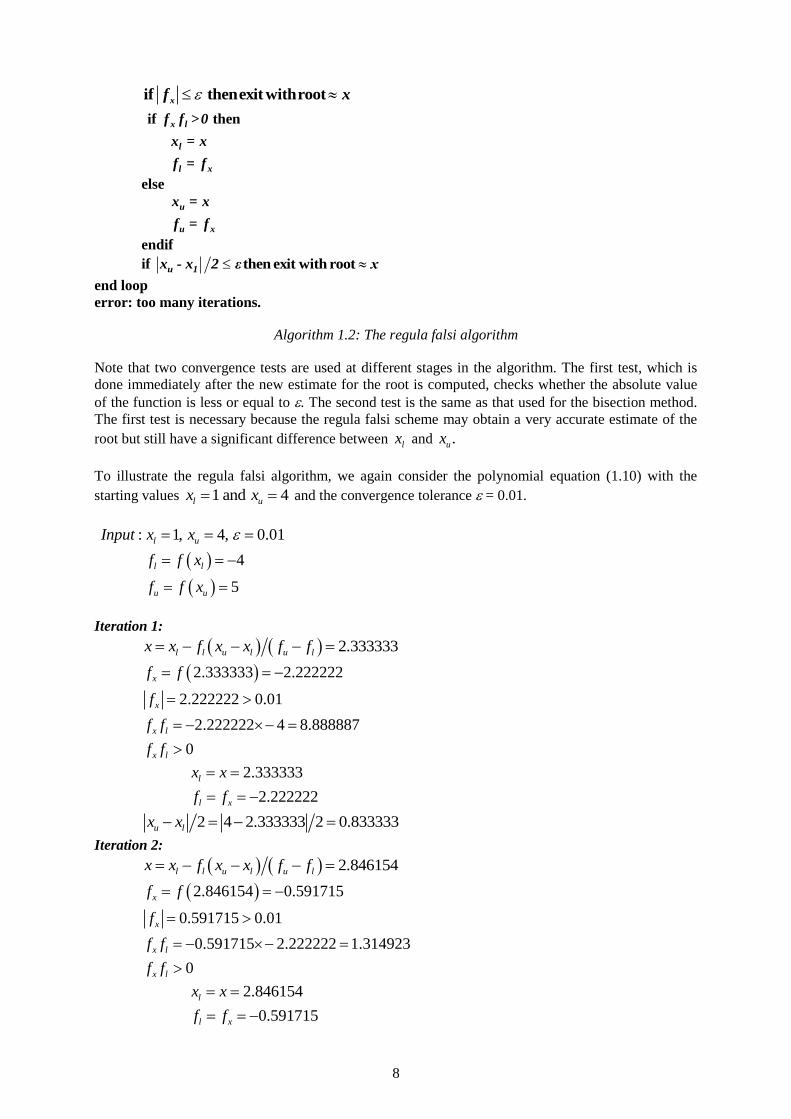
Algorithm 1.2: The regula falsi algorithm

Note that two convergence tests are used at different stages in the algorithm. The first test, which is

done immediately after the new estimate for the root is computed, checks whether the absolute value

of the function is less or equal to . The second test is the same as that used for the bisection method.

The first test is necessary because the regula falsi scheme may obtain a very accurate estimate of the

root but still have a significant difference between lx and .ux

To illustrate the regula falsi algorithm, we again consider the polynomial equation (1.10) with the

starting values 1 and 4l ux x and the convergence tolerance = 0.01.

: 1, 4, 0.01

4

5

l u

l l

u u

Input x x

f f x

f f x

Iteration 1:

2.333333l l u l u lx x f x x f f

2.333333 2.222222

2.222222 0.01

2.222222 4 8.888887

0

x

x

x l

x l

f f

f

f f

f f

2.333333

2.222222

l

l x

x x

f f

2 4 2.333333 2 0.833333u lx x

Iteration 2:


2.846154 0.591715

0.591715 0.01

0.591715 2.222222 1.314923

0

x

x

x l

x l

f f

f

f f

f f

2.846154

0.591715

l

l x

x x

f f

9

2 4 2.846154 2 0.576923u lx x

Iteration 3:


2.968254 0.125977

0.125977 0.01

0.125977 0.591715 0.074543

0

x

x

x l

x l

f f

f

f f

f f

2.968254

0.125977

l

l x

x x

f f

2 4 2.968254 2 0.515873u lx x

Iteration 4:


2.993610 0.025519

0.025519 0.01

0.025519 0.125977 0.003215

0

x

x

x l

x l

f f

f

f f

f f

2.993610

0.025519

l

l x

x x

f f

2 4 2.993610 2 0.503195u lx x

Iteration 5:


2.998720 0.005117

0.0051187 0.01 2.998720

x

x

f f

f exit with root

The convergence of the regula falsi algorithm is shown in Figure 1.7.

Figure 1.7: Convergence of regula falsi algorithm

10

It requires only 5 iterations to converge, compared with the 8 iterations needed for the bisection

scheme. Note that the algorithm terminates with a small value for ,f x even though the difference

between andl ux x is still fairly large.

1.4 Pegasus Algorithm

The regula falsi algorithm may converge slowly if linear interpolation does not estimate the location

of the root accurately. Such cases occur when the iterations approach the root from one side only, as

shown in Figure 1.8. This type of behaviour was indeed observed in the previous example.

Figure 1.8: Problem case for regula falsi algorithm

Figure 1.9: Pegasus algorithm

In the Pegasus algorithm, shown in Figure 1.9, we again assume that the function is linear over the

interval ,l ux x so that the improved estimate for the root is given by equation (1.11). However, if the

function has the same sign for two successive root estimates, uf x is replaced by ug f x where

1 and 0 1,l lg f x f x f x g before proceeding to the next iteration. The same type of

correction is also applied at the other end of the interval when necessary. At all times, the root

remains bracketed. The effect of this simple change, as shown in Figure 1.9, is to accelerate the

convergence of the regula falsi scheme by shifting the estimate toward the true root. An efficient

implementation of the Pegasus scheme is given in Algorithm 1.3.

11

Pegasus Algorithm



l lf = f x

u uf = f x

loop i = 1 to M

l l u l u l

x

x = x - f x - x f f

f = f x

if thenexit withrootf xx

if thenx l

u u l l x

f f >0

f = f f f + f

else

u l

u l

x = x

f = f

endif

l

l x

x = x

f = f

if then exit with rootu ex - x 2 ε x

end loop


Algorithm 1.3: Pegasus algorithm

The above implementation is not obvious and needs study to be understood. The algorithm uses the

fact that the linear interpolation formula of (1.11) can be used to obtain the new estimate for x,

regardless of whether ux is greater or smaller than .lx

To illustrate the Pegasus algorithm, we again consider the polynomial equation (1.10) with the

starting values 1 and 4l ux x and the convergence tolerance = 0.01.

: 1, 4, 0.01

4

5

l u

l l

u u

Input x x

f f x

f f x

Iteration 1:

2.333333

2.333333 2.222222

2.222222 0.01

l l u l u lx x f x x f f

f x f

f x

2.222222 4 8.888887lf x f x

0lf x f x

3.214286u u l l xf f f f f

2.333333

2.222222

2 4 2.333333 2 0.833333

l

l

u l

x x

f f x

x x

12

Iteration 2:

3.014599

3.014599 0.058608

0.058608 0.01

0.058608 2.222222 0.130239

0

l l u l u l

l

l

x x f x x f f

f x f

f x

f x f x

f x f x

2.333333

2.222222

u l

u l

x x

f f

3.014599

0.058608

2 2.333333 3.014599 2 0.340633

l

l

u l

x x

f f x

x x

Iteration 3:

2.997093

2.997093 0.011620

0.011620 0.01

0.011620 0.0558608 0.000681

0

l l u l u l

l

l

x x f x x f f

f x f

f x

f x f x

f x f x

3.014599

0.058608

u l

u l

x x

f f

2.997093

0.011620

2 3.014599 2.997093 2 0.008753

l

l

u l

x x

f f x

x x

0.008753 0.01 2.997093exit withroot

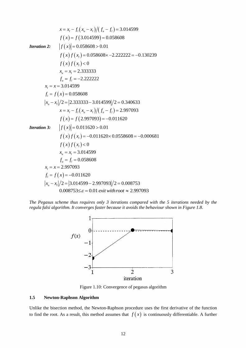
The Pegasus scheme thus requires only 3 iterations compared with the 5 iterations needed by the

regula falsi algorithm. It converges faster because it avoids the behaviour shown in Figure 1.8.

Figure 1.10: Convergence of pegasus algorithm

1.5 Newton-Raphson Algorithm

Unlike the bisection method, the Newton-Raphson procedure uses the first derivative of the function

to find the root. As a result, this method assumes that f x is continuously differentiable. A further

13

difference is that the algorithm only needs a single starting value in order to begin the iteration

process. Provided this starting value is fairly close to the true root, the convergence of the Newton-

Raphson technique is extremely rapid.

With reference to Figure 1.11, we see that, for a given 0x , a better estimate for the root is x, defined by

0

0

0 1

f xf x

x x

Rearranging to isolate 1x gives

0

1 0

0

f xx x

f x

(1.12)

Equation (1.12), which defines the updated estimate for the root, may be written as a more general

recurrence relation according to

1

1

1

i

i i

i

f xx x

f x

(1.13)

Figure 1.11: The Newton-Raphson algorithm

where ix is the ith iteration, which is generated from the 1th

i iteration using (1.13). An initial

guess 0x is required to start the iterations. In the usual form of the Newton-Raphson method, it is

necessary to compute f x explicitly as indicated in Algorithm 1.4.

Newton-Raphson Algorithm

In: Initial guess 0x , tolerance , maximum number of iterations M.


loop i = 1 to M

0 0 0x = x - f x f x

if thenexit withrootf x x

0x = x

end loop


Algorithm 1.4: Newton-Raphson Algorithm

14

Unlike the bisection and regula falsi algorithms discussed previously, the Newton procedure does not

maintain two values which bracket the root. This means that the iterations may become unstable, as

shown in Figure 1.12, or enter a nonconvergent cycle, as shown in Figure 1.13.

Figure 1.12: Divergent Newton-Raphson iterations

Figure 1.13: Nonconvergent cycle of Newton-Raphson iterations

This potential disadvantage, however, is counteracted by its speed of convergence. The method

typically doubles the number of significant figures with each iteration which, for many problems,

means that only three or four iterations are needed to obtain an accurate solution.

Because of the potential instability of the Newton scheme, it is generally prudent to ensure that a good

initial guess for the root is supplied. In some cases, it is beneficial to first use one of the previous

methods with a coarse tolerance to obtain a rough estimate of the root. This can then be improved

using the Newton method.

To illustrate the Newton algorithm we again consider the polynomial equation (1.10) with the starting

value 0 4x and the convergence tolerance 0.01.

Input: 0 4, 0.01x

Iteration 1:

0 0 0

0

3.166667

0.694445 0.01

3.166667

x x f x f x

f x

x x

Iteration 2:

0 0 0

0

3.006410

0.025681 0.01

3.006410

x x f x f x

f x

x x

Iteration 3:

15

0 0 0 3.000010

0.000041 0.01 3.000010

x x f x f x

f x exit with root

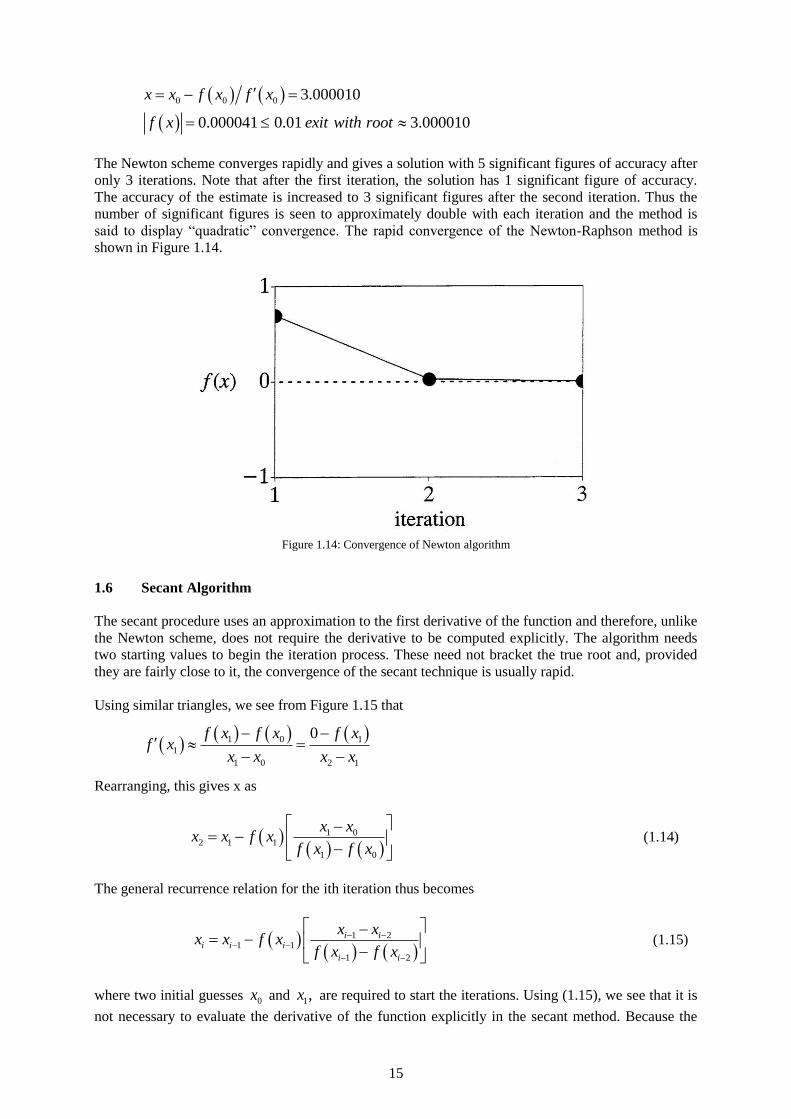
The Newton scheme converges rapidly and gives a solution with 5 significant figures of accuracy after

only 3 iterations. Note that after the first iteration, the solution has 1 significant figure of accuracy.

The accuracy of the estimate is increased to 3 significant figures after the second iteration. Thus the

number of significant figures is seen to approximately double with each iteration and the method is

said to display “quadratic” convergence. The rapid convergence of the Newton-Raphson method is

shown in Figure 1.14.

Figure 1.14: Convergence of Newton algorithm

1.6 Secant Algorithm

The secant procedure uses an approximation to the first derivative of the function and therefore, unlike

the Newton scheme, does not require the derivative to be computed explicitly. The algorithm needs

two starting values to begin the iteration process. These need not bracket the true root and, provided

they are fairly close to it, the convergence of the secant technique is usually rapid.

Using similar triangles, we see from Figure 1.15 that

1 0 1

1

1 0 2 1

0f x f x f xf x

x x x x

Rearranging, this gives x as

1 02 1 1

1 0

x xx x f x

f x f x

(1.14)

The general recurrence relation for the ith iteration thus becomes

1 21 1

1 2

i ii i i

i i

x xx x f x

f x f x

(1.15)

where two initial guesses 0x and 1,x are required to start the iterations. Using (1.15), we see that it is

not necessary to evaluate the derivative of the function explicitly in the secant method. Because the

16

secant procedure does not maintain two values which bracket the root, the iterations may become

unstable. This feature demands that good initial guesses for the root are supplied to ensure

convergence. The secant procedure converges rapidly, but slightly less so than the Newton method.

An efficient implementation of the Secant algorithm is shown in Algorithm 1.5.

Figure 1.15: The secant algorithm

Secant Algorithm

In: Initial guesses 0x and 1x , tolerance , maximum number of iterations M.


0 0f = f x

1 1f = f x

loop i = 1 to M

0 01 1 1 1x = x - f x - x f f

if thenexit withrootf x x

0 1

0 1

1

1

x = x

f = f

x = x

f = f x

end loop


Algorithm 1.5: Secant algorithm

To illustrate the secant algorithm we again consider the polynomial equation (1.10) with the starting

values 0 11 and 4x x and the convergence tolerance = 0.01.

0 1

0 0

1 1

: 1, 4, 0.01

4

5

Input x x

f f x

f f x

Iteration 1:

17

1 1 1 0 1 0

0 1

0 1

1

1

2.333333

2.222222 0.01

4

5

2.333333

2.222222

x x f x x f f

f x

x x

f f

x x

f f x

Iteration 2:

1 1 1 0 1 0

0 1

0 1

1

1

2.846154

0.591715 0.01

2.333333

2.222222

2.846154

0.591715

x x f x x f f

f x

x x

f f

x x

f f x

Iteration 3:

1 1 1 0 1 0

0 1

0 1

1

1

3.032258

0.130073 0.01

2.846154

0.591715

3.032258

0.130073

x x f x x f f

f x

x x

f f

x x

f f x

Iteration 4:

`

1 1 1 0 1 0 2.998720

0.005117 0.01 2.998720

x x f x x f f

f x exit with root

Figure 1.16: Convergence of secant algorithm

Thus the secant scheme meets the convergence tolerance on f x after 4 iterations. When the

derivative of the function is difficult to evaluate, the secant scheme is an attractive alternative to the

Newton method. The convergence rate of the two methods is very similar, although the secant scheme

is not quite quadratic. Figure 1.16 illustrates the variation of f x with iteration number for the

secant scheme.

18

1.7 Comparison of Algorithms for Nonlinear Equations

Key features of the various methods for solving a single nonlinear equation are summarised in Table

1.1. If stability is of the utmost importance, the Pegasus algorithm is a good choice for many

applications. For all continuous functions f x , this method is unconditionally stable and has fast

convergence. For well behaved continuous functions which are continuously differentiable, the

Newton scheme offers quadratic convergence and is generally the fastest of all the methods. It is

essential, however to furnish sound initial guesses for this algorithm if divergence problems are to be

avoided.

Method Initial Values

Required

Derivative

Required Root Bracketing

Speed of

Convergence

bisection 2 no

yes

very stable slow

regula falsi 2 no

yes

very stable medium

Pegasus 2 no

yes

very stable fast

Newton 1 yes

no

conditionally stable very fast

secant 2 no

no

conditionally stable fast

Table 1.1 Features of algorithms for nonlinear equations

1.8 Precision

When designing error and convergence tests for numerical algorithms, it is essential to have a

knowledge of the precision of the numbers that you are using. Precision is critically important for real

numbers, since these are stored only approximately in the computer due to its finite number system.

Roundoff errors also occur when the machine adds, subtracts, multiplies and divides numbers. The

influence of both of these types of error is reduced when the numbers are stored with high precision.

In most computers, integer and real numbers are stored as words which, in turn, are comprised of

bytes. At the next level down, bytes are comprised of bits. To store a number certain bits are reserved

to hold the sign, the exponent, the sign of the exponent, and the mantissa. The number of bits in the

mantissa defines the precision of a real number. The number of bits in the exponent defines the range

of the computer number system; that is the size of the largest and the smallest number that can be

represented on the machine. For numerical work, the precision of the computer number system is

usually of more concern than its range. In most languages, the default precision for real numbers on a

32 bit computer is about 7 decimal places. For large scale calculations this level of precision is not

sufficient, and many languages, such as FORTRAN and C, have double precision (long) reals which

typically give about 16 decimal places. In some extreme cases, where roundoff error is a serious

problem, it is also possible to use quadruple precision.

The level of precision affects the choice of the tolerance that can be used in all of the previous

algorithms. If all quantities are of the order of unity, typical values for would be in the range 410

to 610 for single precision on a 32 bit computer. It would be inappropriate to try and enforce a very

stringent tolerance of, say, 1010

in this case as the machine may be unable to satisfy this value. For

double precision on a 32 bit computer, much tighter values, such as 1210

to 1410

, may be specified

with safety.

Absolute and Relative Error

In numerical computation it is useful to quantify the notion of error. The simplest type of error is

known as absolute error and is defined as

19

true value approximate value (1.16)

This type of error measure can be misleading. Consider the case where the true value = 1000 and the

approximate value = 999. Although the absolute error is 1, the approximation is fairly accurate.

However, if the true value = 1 and the approximate value = 2, then the absolute error is again 1 but the

approximation is very inaccurate. This inconsistency arises because the test is dependent on the scales

of the numbers being used.

The second type of error, known as relative error, is defined as

true value approximate value

true value

(1.17)

Unlike the absolute error test, this type of error measure is insensitive to the scale of the numbers

being tested. It can be used for numbers of widely varying magnitudes and is a good estimator of the

accuracy of an approximation. In the above example, where the true value = 1000 and the approximate

value = 999, the relative error is 31 10 . This indicates that the approximation is relatively accurate.

When the true value = 1 and the approximate value = 2, however, the relative error is 1 which

indicates that the approximation is very inaccurate. Because of its scale independence, the relative

error measure is generally preferable to the absolute error measure. One important exception to this

rule occurs when the true value is zero or very small. In this case, the use of (1.17) may lead to an

arithmetic error due to division by zero or division by a small number.

1.10 The Concept of Significant Figures

The concept of significant figures is used to gauge the accuracy of an approximate value and is

related to the notion of relative error. Formally, the number x* is defined to approximate the true value

x to t significant digits if

*

5 10 tx x

x

(1.18)

where t is a non negative integer. For example, if x = 1000 and x* = 999.4, then

41000 999.4

6 101000

(1.19)

35 10 (1.20)

and x* approximates x to 3 significant figures. Similarly, if x = 1000 and x* = 999.6, then

41000 999.6

4 101000

(1.21)

45 10 (1.22)

and x* is said to approximate x to 4 significant figures. The number of significant figures indicates

how many leading digits in the approximation can be “trusted”. The concept is important in designing

error traps and convergence tests for numerical algorithms, where the exact solution is usually

unknown.

1.11 Testing for Convergence

In all of the previous iteration schemes, we need a test (or tests) to decide when the iterative

solution is sufficiently close to the true solution. This is not as trivial as it may seem, and often causes

20

problems in practical calculations. Letting the subscript i denote iteration number and a small

tolerance, a number of choices for testing convergence may be developed.

One of the simplest criteria uses the absolute change in successive iterates as shown below

1i ix x (1.23)

This test assumes that if the values of x are not changing very much from one iteration to the next,

then the current solution must be quite close to the true solution. This assumption is usually a

reasonable one, although the criterion may sometimes signal premature convergence if the iterative

changes in the solution are small but not changing rapidly with i. A key problem with using the

absolute error test is that the tolerance has to be chosen to reflect the magnitude of the solution x. For

example, if the solution was found to be of the order of 1210 , it would be inappropriate to use a

tolerance of 610 as this would demand roughly 18 decimal places of accuracy in the arithmetic

involving the mantissa.

Instead of using the absolute change, we can check the relative change in successive iterates

according to

1i i

i

x x

x

(1.24)

This criterion also assumes that small changes in the iterates for x imply that the current solution is

quite close to the true solution, but has the extra advantage of being scale independent because it uses

a relative, rather than absolute, error measure. Moreover, comparing equation (1.24) with equation

(1.18), we see that the test gives a rough estimate of the number of significant figures in the solution

(assuming that ix is relatively close to the true solution). Note that this type of criterion cannot be

applied to cases where the root approaches zero, since this may lead to problems with division by zero

or arithmetic overflow (where the root is very small but not identically zero).

In practical codes, it is usual to combine the tests of (1.23) and (1.24) into a single criterion known

as a mixed convergence test. This takes the form

1i i rel i absx x x (1.25)

where andrel abs are, respectively, relative and absolute error tolerances. Whenever ix approaches

zero, the mixed test is essentially an absolute criterion of the form of equation (1.23). For large values

of ix , however, it becomes a relative test of the form of (1.24). This type of test is very robust and

works for all ranges of x values. Using precision arithmetic on a 32-bit machine, typical settings for

andrel abs are in the range 4 610 to 10 .

For algorithms which maintain two bounds that bracket the root, such as the regula falsi and

Pegasus methods, the absolute difference in the bounds can be used to test convergence according to

u lx x (1.26)

Although simple, this test has the same drawbacks as (1.23) in that it is scale dependent. To overcome

this disadvantage, the relative difference in the bounds can be used in the form

u l

u

x x

x

(1.27)

with the restriction that 0.ux In practice, this type of test should not be used if ux is likely to be

small. In practice, the tests (1.26) and (1.27) are often combined into a single mixed bounds test of the

form

21

u l rel u absx x x (1.28)

This type of criterion has the same characteristics and advantages as (1.25), and similar values for the

tolerances andrel abs are used.

Finally, the absolute value of the function can be used as a test for convergence according to

if x (1.29)

Since our aim is to find x such that 0f x , this test has the dual advantages of being both simple

and direct. Unfortunately, it can indicate premature convergence for cases where large changes in x

give only small changes in .f x This occurs when 0f x at the root and is not especially

uncommon. A related problem can arise if the same absolute error test is used for x and for f x as

in several of the algorithms of the Chapter. If the units of f x are different from those of x, then

either the common test for convergence should be relative, or separate values of should be used.

Other tests may also be devised. In many practical codes, it is usual to use a combination of tests to

ensure that true root has been correctly identified.

Computer Lab. MATLAB tutorial: Solving the friction factor equation.

One of the many empirical relations between the friction factor f and the Reynolds number,

Re, for fully developed pipe flow, is

90.010

)(

2332631.0)(log873.1

1

fRefRe

f (1.1)

This relationship can be used to determine the pressure drop in a pipe network and hence

the size of the pump required to drive the flow.

For iteratively solving this equation, an appropriate starting value f0, for at any Re is given

by

2

9.0

100 )/74.5(log25.0

Ref (1.2)

To check your analysis: when Re = 104, f = 0.0324, and for Re = 10

6, f = 0.0119.

Matlab has the function fzero to determine the roots of a function of a single variable. You

can find out about fzero in the main Matlab window (with the prompt >>) by typing

>> help fzero

as you can for most of the Matlab functions and tools. To invoke the function,

>> f = fzero(‘fname’, f0)

22

where f is the root, fname is the function name, and f0 is an initial guess. This command

will automatically print the value of f, whereas

>> f = fzero(‘fname’, f0);

will store the answer in f without printing it. An alternative way of invoking the function is

through the “function handle” @:

>> f = fzero(@fname, f0);

Matlab purists generally prefer function handles. The easiest way to use fzero is to have

two auxiliary M-files, the first to obtain f0, and then the function given by (1.1). M-files

are a simple way of storing Matlab commands or evaluations so that they do not have to be

continually retyped. An M-file is created by selecting File in the Matlab window, then

New and then M-file. The M-file to give the initial guess from (1.2) has the following

contents:

function fric_0 = friction_0(Re) % All comments are preceded by a percentage sign

fric_0 = 0.25/(log10(5.74/Re^0.9))^2; % The semi-colon (;) prevents fric_0 being printed when the function is invoked.

and the file must be saved as friction_0.m. The file is then executed in the Matlab window

by

>>friction_0(10000)

which will return the answer 0.0310. If instead you use

>>f0 = friction_0(10000)

then f0 will hold the initial guess for the friction factor which can then be used in fzero.

fzero uses a mixture of root finding algorithms, but in its simplest form is limited to

functions of only one variable. Thus the M-file that evaluates (1) for the friction factor

cannot have Re as a function argument: it must be set in the function. (This problem does

not arise for Equation (2).) The outline of the methods used by fzero is:

Find xu and xl as so that f(xu) and f(xl) have opposite signs

Use the Secant method to find new x as approximation to the root

Repeat until convergence is achieved

Arrange xu, xl, and x so that f(xu) and f(xl) have opposite signs, | f(xu) | | f(xl) |, and

x is the previous value of xu.

If x xl, consider using the “inverse quadratic interpolation” algorithm which we

have not studied

If x = xl, consider using the Secant method

If either of the two previous steps give a solution in the interval [xu, xl] take the step,

otherwise use bisection again.

23

(This information about fzero comes from Chapter 4 of Cleve Moler “Numerical

Computing with Matlab” which is freely available from www.mathworks.com/moler.

Moler has developed a large number of the Matlab routines.)

Write an M-file that will solve (1) for f, noting that the form of the function must be F(f) =

0 and that the mathematical function sqrt(x) in Matlab returns the square root of x. If you

call your function friction, then you can now solve (1) by a statement similar to

>> f = fzero(‘friction’, f0)

You can also plot the function using the Matlab routine plot. One way to do this is to write

another M-file, called, say, plot_frict.m. Type the following into the file:

for k = 1:1:10 x(k) = 0.03 + (k-1)*.001; %values appropriate to Re = 1.e4 y(k) = friction(x(k)); end plot(x, y, 's-')

for Re = 10

4. Note that the code beginning “for” and ending “end” is Matlab’s way of

looping. The “loop variable” k has the successive values: 1, 2, 3, 4, … Note also that an M-

file may reference another M-file (friction.m in this case).

Then in the Matlab window

>> plot_frict

and a plot of the function going through zero should appear in a separate window. Under

“Edit” and “Axes Properties” you should find how to turn on the grid for the plot which

will show more clearly where the function goes through zero. Use help plot to figure out

the meaning of 's-'.

Exercises

1. Rewrite friction.m and plot_frict.m to plot the values of f going through zero for Re = 10

6.

2. Repeat the calculations using

>> f = fzero(‘friction’, f0, optimset(‘disp’, ‘iter’))

which gives information about how Matlab searches for the root and how many

iterations it requires. Check help fzero and help optimset for information on these

options. Relate the information to the outline of fzero given on the previous page.

3. Repeat Part with f0 replaced by 0.02, 0.04, 0.1 0.2, etc until Matlab cannot find the

root. Note how the number of iterations increases as the initial guess moves further

away from the root.

4. It is possible (in a somewhat roundabout way) to pass the Reynolds number to a

modified version of friction.m using

>> f = fzero(‘friction’, f0, [], Re);

Try modifying friction.m to do this.

http://www.mathworks.com/moler

24

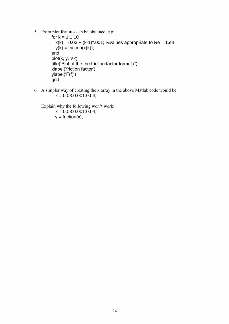
5. Extra plot features can be obtained, e.g:

for k = 1:1:10 x(k) = 0.03 + (k-1)*.001; %values appropriate to Re = 1.e4 y(k) = friction(x(k)); end plot(x, y, 's-') title(‘Plot of the the friction factor formula”) xlabel(‘friction factor’) ylabel(‘F(f)’) grid

6. A simpler way of creating the x array in the above Matlab code would be

x = 0.03:0.001:0.04;

Explain why the following won’t work:

x = 0.03:0.001:0.04; y = friction(x);

1 Solution of a Non-Linear Equation

Documents

Transcript of 1 Solution of a Non-Linear Equation