
Solution of the fully fuzzy linear systems using iterative techniques
21
Solution of the fully fuzzy linear systems using iterative techniques Mehdi Dehghan * , Behnam Hashemi, Mehdi Ghatee Department of Applied Mathematics, Faculty of Mathematics and Computer Science, Amirkabir University of Technology, No. 424, Hafez Avenue, Tehran 15914, Iran Accepted 17 March 2006 Communicated by Professor Gerando Iovane Abstract This paper mainly intends to discuss the iterative solution of fully fuzzy linear systems which we call FFLS. We employ Dubois and Prade’s approximate arithmetic operators on LR fuzzy numbers for finding a positive fuzzy vector ~ x which satisfies e A~ x ¼ e b, where e A and e b are a fuzzy matrix and a fuzzy vector, respectively. Please note that the pos- itivity assumption is not so restrictive in applied problems. We transform FFLS and propose iterative techniques such as Richardson, Jacobi, Jacobi overrelaxation (JOR), Gauss–Seidel, successive overrelaxation (SOR), accelerated over- relaxation (AOR), symmetric and unsymmetric SOR (SSOR and USSOR) and extrapolated modified Aitken (EMA) for solving FFLS. In addition, the methods of Newton, quasi-Newton and conjugate gradient are proposed from non- linear programming for solving a fully fuzzy linear system. Various numerical examples are also given to show the effi- ciency of the proposed schemes. Ó 2006 Elsevier Ltd. All rights reserved. 1. Introduction Since many real-world engineering systems are too complex to be defined in precise terms, imprecision is often involved. Analyzing such systems requires the use of fuzzy information. Fuzzy sets can provide solutions to a broad range of prob- lems of fuzzy topological spaces [5], hyperchaotic systems [33], quantum optics [12], medicine [1], and so on. Friedman and his colleagues proposed a general model for solving a fuzzy linear system of which the coefficient matrix is crisp and the right-hand side column is an arbitrary fuzzy vector for the first time [14]. They used the embed- ding method and replaced the original fuzzy linear system by a crisp linear system and then they solved it. But what happens if all parameters in a fuzzy linear system be fuzzy numbers, which we call a fully fuzzy linear system (denoted by FFLS) and what is the solution of this kind of fuzzy linear systems? Dubois and Prade investigated two definitions of a system of fuzzy linear equations, one consisting of a system of tolerance constraints, the other of approximate equalities in [10]. Buckley et al. [4] discussed the theoretical aspects of the 0960-0779/$ - see front matter Ó 2006 Elsevier Ltd. All rights reserved. doi:10.1016/j.chaos.2006.03.085 * Corresponding author. Tel.: +98 21 6406322; fax: +98 21 6497930. E-mail addresses: [email protected] (M. Dehghan), [email protected] (B. Hashemi), [email protected] (M. Ghatee). Chaos, Solitons and Fractals 34 (2007) 316–336 www.elsevier.com/locate/chaos
Transcript of Solution of the fully fuzzy linear systems using iterative techniques

Chaos, Solitons and Fractals 34 (2007) 316–336
www.elsevier.com/locate/chaos
Solution of the fully fuzzy linear systems usingiterative techniques
Mehdi Dehghan *, Behnam Hashemi, Mehdi Ghatee
Department of Applied Mathematics, Faculty of Mathematics and Computer Science, Amirkabir University of Technology,
No. 424, Hafez Avenue, Tehran 15914, Iran
Accepted 17 March 2006
Communicated by Professor Gerando Iovane
Abstract
This paper mainly intends to discuss the iterative solution of fully fuzzy linear systems which we call FFLS. Weemploy Dubois and Prade’s approximate arithmetic operators on LR fuzzy numbers for finding a positive fuzzy vector~x which satisfies eA~x ¼ eb, where eA and eb are a fuzzy matrix and a fuzzy vector, respectively. Please note that the pos-itivity assumption is not so restrictive in applied problems. We transform FFLS and propose iterative techniques suchas Richardson, Jacobi, Jacobi overrelaxation (JOR), Gauss–Seidel, successive overrelaxation (SOR), accelerated over-relaxation (AOR), symmetric and unsymmetric SOR (SSOR and USSOR) and extrapolated modified Aitken (EMA)for solving FFLS. In addition, the methods of Newton, quasi-Newton and conjugate gradient are proposed from non-linear programming for solving a fully fuzzy linear system. Various numerical examples are also given to show the effi-ciency of the proposed schemes.� 2006 Elsevier Ltd. All rights reserved.
1. Introduction
Since many real-world engineering systems are too complex to be defined in precise terms, imprecision is often involved.Analyzing such systems requires the use of fuzzy information. Fuzzy sets can provide solutions to a broad range of prob-lems of fuzzy topological spaces [5], hyperchaotic systems [33], quantum optics [12], medicine [1], and so on.
Friedman and his colleagues proposed a general model for solving a fuzzy linear system of which the coefficientmatrix is crisp and the right-hand side column is an arbitrary fuzzy vector for the first time [14]. They used the embed-ding method and replaced the original fuzzy linear system by a crisp linear system and then they solved it. But whathappens if all parameters in a fuzzy linear system be fuzzy numbers, which we call a fully fuzzy linear system (denotedby FFLS) and what is the solution of this kind of fuzzy linear systems?
Dubois and Prade investigated two definitions of a system of fuzzy linear equations, one consisting of a system oftolerance constraints, the other of approximate equalities in [10]. Buckley et al. [4] discussed the theoretical aspects of the
0960-0779/$ - see front matter � 2006 Elsevier Ltd. All rights reserved.doi:10.1016/j.chaos.2006.03.085
* Corresponding author. Tel.: +98 21 6406322; fax: +98 21 6497930.E-mail addresses: [email protected] (M. Dehghan), [email protected] (B. Hashemi), [email protected] (M. Ghatee).

M. Dehghan et al. / Chaos, Solitons and Fractals 34 (2007) 316–336 317
problem through the development of several theorems related to the existence of a solution. But their work may notrepresent a numerical tool for practical implementation in the context of engineering systems [28]. Although otherinvestigations have been reported in the literature on the solution of fuzzy systems [16,34,24], but very few methodsare available for the practical solution of a FFLS. The main reason of this drawback is their structure. With a moreclear statement, as mentioned by Kreinovich et al. [25] finding a solution of a system with interval coefficient is NP-hard. Based on their important results, it is trivial that obtaining the same solution of a FFLS is not easy. Differentfrom this practical point of view, Rao and Chen [28] provided a computational method to systematically solve a setof fuzzy linear equations, based on the specified a-level cuts. In this paper we intend to solve the fuzzy linear systemeA � ~x ¼ ~b, where eA is a fuzzy matrix and ~x and ~b are fuzzy vectors with appropriate sizes. These systems are usefulin the analysis of biological and physical systems and other topics in real engineering problems, where uncertaintyaspects appear, for instance the finite element formulation of equilibrium and steady state problems which lead to aset of simultaneous algebraic linear equations [28]. The term fuzzy matrix, which is the most important concept in thispaper, has various meanings in the literature. For definition of a fuzzy matrix we use the definition of Dubois and Pradein [11] i.e., a matrix with fuzzy numbers as its elements [10,11]. These fuzzy matrices can model uncertain and vagueaspects, and the researches on them are mostly limited. We limit our attention on fuzzy matrices and employ Duboisand Prade arithmetic operators as mentioned in [11,15,30]. Recently Dehghan et. al, proposed Cramer’s rule, Gaussianelimination and fuzzy LU decomposition (Doolittle algorithm) for solving FFLS. They also showed the applicability ofthe linear programming approach for over-determined FFLS in [7].
Iterative methods for solving linear systems have along history, going back at least to Gauss. In this paper we focuson the iterative solution of FFLS with some well-known iterative methods such as Jacobi, Gauss–Seidel, SOR, AOR,SSOR, USSOR and EMA.
In Section 2, we define FFLS and its solution based on the basic materials from fuzzy set theory which is presented inAppendix A. In Section 3, we construct some classic iterative methods for solving FFLS. Then we will representiterative methods for solving a FFLS, using splitting approach in Section 4. In Section 5, using some methods fromnonlinear programming, we will try to offer a solution for the FFLS. Section 6 contains stability and error analysison numerical examples. The final section ends this paper with a brief conclusion.
2. Fully fuzzy linear systems and their solutions
Definition 2.1. A matrix eA ¼ ðfaijÞ is called a fuzzy matrix, if each element of eA is a fuzzy number [10,11].eA will be positive (negative) and denoted by eA > 0 ðeA < 0Þ if each element of eA be positive (negative). Similarly,non-negative and non-positive fuzzy matrices may be defined.
Let each element of eA be a LR fuzzy number. We may represent eA ¼ ðfaijÞ that faij ¼ ðaij; aij; bijÞLR, with new nota-tion eA ¼ ðA;M ;NÞ; where A, M and N are three crisp matrices, with the same size of eA, such that A = (aij), M = (aij)and N = (bij), are called the center matrix and the right and left spread matrices, respectively.
Definition 2.2. A square fuzzy matrix eA ¼ faij will be an upper (lower) triangular fuzzy matrix, if
faij ¼ e0 ¼ ð0; 0; 0Þ; 8i > j ð8i < jÞ:
Definition 2.3. Let eA ¼ ðfaijÞ and eB ¼ ðfbijÞ be two m · n and n · p fuzzy matrices. We define eA � eB ¼ eC ¼ ðfcijÞ which isthe m · p matrix where
fcij ¼X�
k¼1;...;n
faik � fbkj :
Up to rest of this paper we use Dubois and Prade’s approximate multiplication �.
Definition 2.4. Consider the n · n linear system of equations:
ðfa11 � ex1Þ � ðfa12 � ex2Þ � � � � � ðfa1n � exnÞ ¼ eb1 ;
ðfa21 � ex1Þ � ðfa22 � ex2Þ � � � � � ðfa2n � exnÞ ¼ eb2 ;
..
.
ðfan1 � ex1Þ � ðfan2 � ex2Þ � � � � � ðfann � exnÞ ¼ ebn :
8>>>>><>>>>>:ð1Þ
318 M. Dehghan et al. / Chaos, Solitons and Fractals 34 (2007) 316–336
The matrix form of the above equations is
eA � ~x ¼ eb; ð2Þ or simply eA~x ¼ eb where the coefficient matrix eA ¼ ðfaijÞ; 1 6 i; j 6 n is a n · n fuzzy matrix and exi ; ebi 2FðE1Þ,1 6 i 6 n. This system is called a fully fuzzy linear system (FFLS). Also, if each element of eA and eb be a positiveLR fuzzy number, we call the system (2) a positive FFLS.To answer the question, ‘‘What is the solution of FFLS?’’, we firstly mention some ideas, in the following way:
1. Let x = (xj)j=1,. . .,n be a crisp vector solution of FFLS with some negative and positive elements.• Let we must find x P 0. In this case, the FFLS translates to the following system:
ðAx;Mx;NxÞ ¼ ðb; g; hÞ:
This system has clearly an exact solution if and only if the vector x be the solution of Ax = b, Mx = g andNx = h, synchronously. Otherwise, the system has not any positive exact solution. But in this case, we can definean approximate solution. This idea is common in real applications, such as solving non-square systems with thepseudo-inverse methods. For implementing this idea in the above system we may use the 2-norm and define apotential function, as follows:
f ðxÞ ¼ ðAx� bÞ2 þ ðMx� gÞ2 þ ðNx� hÞ2:
Ideally, if some x P 0, can be found as the optimal solution of this system by zero value, an exact solution isfound. Else, we could find an approximate solution for this system. Note that if A, M and N be positive definitematrices, then f(x) will be convex function which allow us to implement some powerful methods of nonlinearoptimization, such as iterative methods of Newton and quasi-Newton or conjugate gradient method [3], for find-ing its optimal solution. Consider the following FFLS, for example:
ð2; 1; 1Þx1 þ ð3; 1; 2Þx2 ¼ ð14; 6; 8Þ;ð4; 1; 2Þx1 þ ð5; 2; 2Þx2 ¼ ð26; 8; 12Þ;
�ð3Þ
in which (x1,x2) = (4,2) is its crisp solution.• Let we must find some x 6 0. In this case the original fuzzy system is transformed to the following system,
ðAx;�Nx;�MxÞ ¼ ðb; g; hÞ;
so, the exact solution of system can be found if and only if the vector x be satisfy in Ax = b, Nx = �g andMx = �h, contemporary. Otherwise, the system has not any negative exact solution. Like the discussion above,if we minimize,
f ðxÞ ¼ ðAx� bÞ2 þ ðNxþ gÞ2 þ ðMxþ hÞ2;
we can find exact or approximated negative solution of system when the optimal value be zero or greater thanzero, respectively.
• Let x be neither positive, nor negative. This case is very complicated, because the definition of scaler multiplyingfor positive and negative solution is different. So we should consider two cases for each variable; positive andnegative cases. Thus we must solve 2n crisp systems or corresponding optimization problem, which is not appli-cable to real problems with large scale matrices.
2. Another strategy is finding a vector as the center of solution of FFLS in one step and extending some spreads for itscomponents in the next step, i.e., if c be found as a center, for example, in the second step we find d > 0 that x + dand x � d be the solution of system, too. But solving these systems is as difficult as the previous approach.
3. In many applied problems, engineers had some information about the range of spreads of fuzzy solution. In thesecases with fixed vectors y and z, as the left and right spreads, the original problem is transformed to finding a vectorx which satisfies in the following systems:
Ax ¼ b;
Mx ¼ g � Ay;
Nx ¼ h� Az:
8><>: ð4Þ
Thus, with utilizing pseudo-inverse, we can find x that is the nearest solution for the above systems.For example, consider the FFLS (3) with yt = (1,0.5) and zt = (0.5,0.75) are given fixed left and right spreads, thenthe fuzzy solution
M. Dehghan et al. / Chaos, Solitons and Fractals 34 (2007) 316–336 319
~x ¼ð5:0057; 1; 0:5Þð0:5170; 0:5; 0:75Þ
� �;
can be found.4. Using the cuts instead of fuzzy numbers is a common event in fuzzy computations (see e.g. [28]). The most important
issue of this approach is the basic works on interval systems [19–22]. But solving these systems is not easy in practice.5. The cuts on 0 and 1 are the most important aspects of fuzzy numbers, because the first one presents the bound of
fuzzy numbers and the second one shows the most possible cases. So, we can solve Ax = b, (A �M)xL = b � g and(A + N)xR = b + h, where xL and xR are lower and upper bounds of fuzzy solution, which may be presented asy = x � xL and z = xR � x with our notations.
6. Utilizing the approximation arithmetic operators such as Dubois and Prade’s approach [11] or the idea of Wagen-knecht et al. [30], permit us to mention the error analysis, that will be presented in this article.
Definition 2.5. Consider the positive FFLS (2). ~x is a solution, if and only if
Ax ¼ b;
Mxþ Ay ¼ g;
Nxþ Az ¼ h:
8><>: ð5Þ
In addition, if y P 0, z P 0 and x � y P 0 we say ~x ¼ ðx; y; zÞ is a consistent solution of positive FFLS or for abbrevi-ation consistent solution. Otherwise, it will be called dummy solution.
The final target of this paper is to find the consistent solution of the FFLS. But unfortunately, the proposed algo-rithms (which will be mentioned soon) may converge to the dummy solutions.
2.1. The direct method for solving FFLS
Assuming that A is a non-singular crisp matrix, we can say
ðAx;Ay þMx;Azþ NxÞ ¼ ðb; h; gÞ:
Thus, we have
Ax ¼ b;
Ay þMx ¼ h;
Azþ Nx ¼ g;
8><>:
i.e., we can say,ai1x1 þ ai2x2 þ � � � þ ainxn ¼ bi;
ðai1y1 þ ai2y2 þ � � � þ ainynÞ þ ðmi1x1 þ mi2x2 þ � � � þ minxnÞ ¼ gi;
ðai1z1 þ ai2z2 þ � � � þ ainznÞ þ ðni1x1 þ ni2x2 þ � � � þ ninxnÞ ¼ hi:
8><>: 1 6 i 6 n; ð6Þ
In other words, we have
Ax ¼ b;
Ay ¼ h�Mx;
Az ¼ g � Nx:
8><>: ð7Þ
Thus we easily have
Ax ¼ b) x ¼ A�1b; ð8Þ
and then by this representation in the second and the third equations, we have
y ¼ A�1h� A�1Mx; ð9Þ
and
z ¼ A�1g � A�1Nx: ð10Þ
Theorem 2.6. Let eA ¼ ðA;M ;NÞ and eb ¼ ðb; g; hÞ be a non-negative fuzzy matrix and a non-negative fuzzy vector, and let
A be the product of a permutation matrix by a diagonal matrix with positive diagonal entries. Also, let h P MA�1b,
g P NA�1b and (MA�1 + I)b P h. Then the system eA~x ¼ eb has a positive fuzzy solution.
Proof. Our hypotheses on A, imply that A�1 exists and is a non-negative matrix [8]. So, x = A�1b P 0.On the other hand, h P MA�1b and g P NA�1b. Thus with y = A�1h � A�1Mx and z = A�1g � A�1Nx, we have
y P 0 and z P 0. So ~x ¼ ðx; y; zÞ is a fuzzy vector which satisfies eA~x ¼ eb. Since x � y = A�1(b � h + MA�1b), thepositivity property of ~x can be obtained from (MA�1 + I)b P h. h
320 M. Dehghan et al. / Chaos, Solitons and Fractals 34 (2007) 316–336
3. Iterative methods
In this section we seek for solving the FFLS (7) using iterative methods. These methods lead to the following form
xðkþ1Þ
yðkþ1Þ
zðkþ1Þ
264375 ¼ C
xðkÞ
yðkÞ
zðkÞ
264375þ c ðk P 0Þ; ð11Þ
where C is called the iteration matrix of the iterative method and c is a vector. On the other hand, consider the firstequation of (7), i.e., Ax = b. We use the following decomposition for the center matrix A
A ¼ LA þ DA þ U A; ð12Þ
in which DA is the diagonal of matrix A, LA its strict lower part and UA its strict upper part. It is always assumed thatthe diagonal entries of the crisp matrix A are all non-zero.
Note that we use positive fuzzy numbers and seek for the positive fuzzy solution of FFLS. The positivity assumptionis not so restrictive in applicable problems. Note also that there exist some cases in which eA~x ¼ ~b, but the left spread orright spread of ~x is negative, which is not acceptable.
3.1. Jacobi method
Consider the FFLS eA~x ¼ ~b. Using Eq. (6), we can say
aiixi ¼ bi �Pn
j¼1;j 6¼iaijxj;
aiiyi ¼ gi �Pn
j¼1;j6¼iaijyj þ
Pnj¼1
mijxj
!;
aiizi ¼ hi �Pn
j¼1;j6¼iaijzj þ
Pnj¼1
nijxj
!;
8>>>>>>>>><>>>>>>>>>:1 6 i 6 n;
which suggests the following iterative process as the Jacobi method for solving a FFLS
xðkþ1Þi ¼ 1
aiibi �
Xj 6¼i
aijxðkÞj
!;
yðkþ1Þi ¼ 1
aiigi �
Xj6¼i
aijyðkÞj �
Xn
j¼1
mijxðkÞj
!;
zðkþ1Þi ¼ 1
aiihi �
Xj 6¼i
aijzðkÞj �
Xn
j¼1
nijxðkÞj
!:
8>>>>>>>>>>><>>>>>>>>>>>:1 6 i 6 n; ð13Þ
So, the Jacobi iterative scheme is as follows:
xðkþ1Þ ¼ �D�1A ðLA þ U AÞxðkÞ þ D�1
A b;
yðkþ1Þ ¼ �D�1A ðLA þ U AÞyðkÞ � D�1
A MxðkÞ þ D�1A g;
zðkþ1Þ ¼ �D�1A ðLA þ U AÞzðkÞ � D�1
A NxðkÞ þ D�1A h;
8><>:

M. Dehghan et al. / Chaos, Solitons and Fractals 34 (2007) 316–336 321
where by Eq. (12) the Jacobi iteration matrix is the following block 3n · 3n crisp matrix
CJ ¼�D�1
A ðLA þ U AÞ 0 0
�D�1A M �D�1
A ðLA þ U AÞ 0
�D�1A N 0 �D�1
A ðLA þ U AÞ
264375; ð14Þ
and we have
c ¼D�1
A b
D�1A g
D�1A h
264375:
The stationary iterative methods are relatively easy to program, although there are many issues to consider when com-plicated data structures or parallel computers are used. The MATLAB implementation of the Jacobi iterative methodfor solving FFLS is given in Appendix B. One can use other stopping criteria in this program.
3.2. The forward Gauss–Seidel method
Another well-known method for solving FFLS is the forward Gauss–Seidel iteration. Seidel introduced its classicalversion for solving the crisp linear system Ax = b in 1874. Consider the Eq. (6). Thus, we can say
Pj6iaijxj ¼ bi �
Pnj>i
aijxj;
Pj6i
aijyi ¼ gi �Pnj>i
aijyj þPnj¼1
mijxj
!;
Pj6i
aijzi ¼ hi �Pnj>i
aijzj þPnj¼1
nijxj
!:
8>>>>>>>>><>>>>>>>>>:1 6 i 6 n;
So the forward Gauss–Seidel iterative method will be
xðkþ1Þi ¼ 1
aiibi �
Xn
j<i
aijxðkþ1Þj �
Xn
j>i
aijxðkÞj
" #;
yðkþ1Þi ¼ 1
aiigi �
Xn
j<i
aijyðkþ1Þj �
Xn
j>i
aijyðkÞj �
Xn
j¼1
mijxðkÞj
" #;
zðkþ1Þi ¼ 1
aiihi �
Xn
j<i
aijzðkþ1Þj �
Xn
j>i
aijzðkÞj �
Xn
j¼1
nijxðkÞj
" #;
8>>>>>>>>>>><>>>>>>>>>>>:1 6 i 6 n; k P 0 ð15Þ
or, in the matrix form we have
ðDA þ LAÞxðkþ1Þ ¼ b� U AxðkÞ;
ðDA þ LAÞyðkþ1Þ ¼ g � U AyðkÞ �MxðkÞ;
ðDA þ LAÞzðkþ1Þ ¼ h� U AzðkÞ � NxðkÞ:
8><>:
Thus the forward Gauss–Seidel iterative method for solving FFLS is as follows:xðkþ1Þ ¼ �ðDA þ LAÞ�1U AxðkÞ þ ðDA þ LAÞ�1b;
yðkþ1Þ ¼ �ðDA þ LAÞ�1U AyðkÞ � ðDA þ LAÞ�1MxðkÞ þ ðDA þ LAÞ�1g;
zðkþ1Þ ¼ �ðDA þ LAÞ�1U AzðkÞ � ðDA þ LAÞ�1NxðkÞ þ ðDA þ LAÞ�1h;
8><>:
and the Gauss–Seidel iteration matrix isCGS ¼�ðDA þ LAÞ�1U A 0 0
�ðDA þ LAÞ�1M �ðDA þ LAÞ�1U A 0
�ðDA þ LAÞ�1N 0 �ðDA þ LAÞ�1U A
264375; ð16Þ
322 M. Dehghan et al. / Chaos, Solitons and Fractals 34 (2007) 316–336
and
c ¼ðDA þ LAÞ�1b
ðDA þ LAÞ�1g
ðDA þ LAÞ�1h
264375:
3.3. The forward successive overrelaxation method
Now we introduce the forward SOR method for solving FFLS. Consider the Eq. (2), add and subtract xðkÞi to theright hand side of the first equation of (15), yðkÞi and zðkÞi to the right hand sides of the second and third equations of(15), respectively. Thus we get
xðkþ1Þi ¼ xðkÞi þ 1
aiibi �
Pnj<i
aijxðkþ1Þj �
PnjPi
aijxðkÞj
" #;
yðkþ1Þi ¼ yðkÞi þ 1
aiigi �
Pnj<i
aijyðkþ1Þj �
PnjPi
aijyðkÞj �
Pnj¼1
mijxðkÞj
" #;
zðkþ1Þi ¼ zðkÞi þ 1
aiihi �
Pnj<i
aijzðkþ1Þj �
PnjPi
aijzðkÞj �
Pnj¼1
nijxðkÞj
" #;
8>>>>>>>>>><>>>>>>>>>>:1 6 i 6 n; k P 0
and using the overrelaxation parameter x, the forward SOR iterative method will be
xðkþ1Þi ¼ xðkÞi þ x 1
aiibi �
Pj<i
aijxðkþ1Þj �
PjPi
aijxðkÞj
" #;
yðkþ1Þi ¼ yðkÞi þ x 1
aiigi �
Pj<i
aijyðkþ1Þj �
PjPi
aijyðkÞj �
Pnj¼1
mijxðkÞj
" #;
zðkþ1Þi ¼ zðkÞi þ x 1
aiihi �
Pj<i
aijzðkþ1Þj �
PjPi
aijzðkÞj �
Pnj¼1
nijxðkÞj
" #;
8>>>>>>>>>><>>>>>>>>>>:ð17Þ
where 1 6 i 6 n and k P 0 are integers. Now, consider the first equation in (17). We can say
aiixðkþ1Þi þ x
Xi�1
j¼1
aijxðkþ1Þj ¼ aiix
ðkÞi � x
Xn
j¼i
aijxðkÞj þ xbi;
and so,
aiixðkþ1Þi þ x
Xi�1
j¼1
aijxðkþ1Þj ¼ aiix
ðkÞi � xaiix
ðkÞi � x
Xn
j¼iþ1
aijxðkÞj þ xbi;
i.e., in the matrix form we have
ðDA þ xLAÞxðkþ1Þ ¼ ð1� xÞDAxðkÞ � xU AxðkÞ þ xb;
and since DA + xLA is a lower triangular square matrix with non-zero diagonal elements, it is non-singular and we canutter the first equation of (17) in the following form:
xðkþ1Þ ¼ �ðDA þ xLAÞ�1½ðx� 1ÞDA þ xU A�xðkÞ þ xðDA þ xLAÞ�1b:
Thus, we can determine the matrix form of the forward SOR method for solving FFLS in the following form:
xðkþ1Þ ¼ �ðDA þ xLAÞ�1½ðx� 1ÞDA þ xUA�xðkÞ þ xðDA þ xLAÞ�1b;yðkþ1Þ ¼ �ðDA þ xLAÞ�1½ðx� 1ÞDA þ xU A�yðkÞ � xðDA þ xLAÞ�1MxðkÞ þ xðDA þ xLAÞ�1g;zðkþ1Þ ¼ �ðDA þ xLAÞ�1½ðx� 1ÞDA þ xU A�zðkÞ � xðDA þ xLAÞ�1NxðkÞ þ xðDA þ xLAÞ�1h:
8><>: ð18Þ
Thus the SOR iteration matrix is
CSOR ¼W 0 0
�xðDA þ xLAÞ�1M W 0
�xðDA þ xLAÞ�1N 0 W
24 35;
W ¼ �ðDA þ xLAÞ�1½ðx� 1ÞDA þ xU A�:
ð19Þ
M. Dehghan et al. / Chaos, Solitons and Fractals 34 (2007) 316–336 323
4. The splitting approach for iterative techniques
We now consider iterative methods in a more general mathematical setting. A general type of iterative process forsolving the system (7), can be described as follows. Let A = Q � P be a proper splitting of crisp matrix A and Q, calledthe splitting matrix, be a non-singular crisp matrix. Thus, we obtain the equivalent form
Qx ¼ Pxþ b;
Qy ¼ Py �Mxþ h;
Qz ¼ Pz� Nxþ g;
8><>: ð20Þ
which suggests the following iterative processes
xðkþ1Þ ¼ Q�1PxðkÞ þ Q�1b;
yðkþ1Þ ¼ Q�1PyðkÞ � Q�1MxðkÞ þ Q�1h;
zðkþ1Þ ¼ Q�1PzðkÞ � Q�1NxðkÞ þ Q�1g:
8><>: ð21Þ
The initial vector ~xð0Þ ¼ ðxð0Þ; yð0Þ; zð0ÞÞ can be an arbitrary positive fuzzy vector. If a good guess of the solution is avail-able, it should be used for ~xð0Þ. Our objective is to choose Q so that
(i) the sequence f~xðkÞg is easily computed,(ii) the sequence f~xðkÞg converges rapidly to the solution.
If the iterative processes be convergent, then by taking the limit in Eq. (21), the result is Eq. (20), which means thatAx = b. In the sense of Eq. (11), the matrix
C ¼Q�1P 0 0
�Q�1M Q�1P 0
�Q�1N 0 Q�1P
264375; ð22Þ
is called the iteration matrix. Finally, we have the solution ~x ¼ ðx; y; zÞ in hand. In the following we propose the maintheorem of this paper.
Theorem 4.1. The iterative method (21) for solving fully fuzzy linear system eA~x ¼ eb, converges if and only if its classical
version converges for solving the crisp linear system Ax = b derived from the corresponding FFLS.
Proof. Clearly the iterative method (21) converges if and only if q(C) < 1, where C is its iteration matrix (22). Since it isa block lower triangular crisp matrix, we have
rfCg ¼ rfQ�1Pg;
where r shows the spectrum. Since Q�1P is the iteration matrix of the classical corresponding method for solvingAx = b, the proof is complete. h
4.1. The Richardson method and its extrapolation
As an illustration of the above concepts, we consider the Richardson method, in which the splitting matrix Q is cho-sen to be the identity matrix of order n. Eq. (21) in this case reads as follows:
xðkþ1Þ ¼ ðI � AÞxðkÞ þ b;
yðkþ1Þ ¼ ðI � AÞyðkÞ �MxðkÞ þ h;
zðkþ1Þ ¼ ðI � AÞzðkÞ � NxðkÞ þ g;
8><>: ð23Þ
and the Richardson iteration matrix is
CRich ¼I � A 0 0
�M I � A 0
�N 0 I � A
264375: ð24Þ
In this approach the sequence f~xðmÞg is easily computed, but the rate of convergence of the sequence f~xðmÞg is very slow.
324 M. Dehghan et al. / Chaos, Solitons and Fractals 34 (2007) 316–336
Theorem 4.2. Let the center matrix A be a symmetric positive definite crisp matrix. Then Richardson iterative method (23),
for solving FFLS (2) converges, if and only if l(A) < 2, where l(A) is the largest eigenvalue of A.
Proof. Suppose that the center matrix A, be SPD. So all of the eigenvalues of A will be positive. Note that
qðCRichÞ ¼ maxfj1� lðAÞj; j1� gðAÞjg;
where g(A) and l(A) are the least and the greatest eigenvalues of A, respectively. Now, let the Richardson method con-verge for FFLS, i.e., q(CRich) < 1. Since g(A) < l(A), we have q(A) < 2.
Conversely, let l(A) < 2. Since A is SPD, we have 0 < g(A) < l(A). Thus, we can say
�1 < 1� gðAÞ < 1;
�1 < 1� lðAÞ < 1:
�
So q(CRich) < 1, and the Richardson iterative technique is convergent. hAnother illustration for this basic theory is provided by the ER iteration, in which Q ¼ 1a I , where a is called the
extrapolation parameter. In this case we have:
xðkþ1Þ ¼ ðI � aAÞxðkÞ þ ab;
yðkþ1Þ ¼ ðI � aAÞyðkÞ � aMxðkÞ þ ah;
zðkþ1Þ ¼ ðI � aAÞzðkÞ � aNxðkÞ þ ag;
8><>: ð25Þ
and so the ER iteration matrix is
CER ¼I � aA 0 0
�aM I � aA 0
�aN 0 I � aA
264375: ð26Þ
Corollary 1. Using Theorem 4.1 of this paper and the discussions presented in [18, p. 23] , it is easy to show that if the
center matrix A is symmetric positive definite, then the optimum extrapolation parameter would be aopt ¼ 2mðAÞþMðAÞ, and in
this case we have qð.ERaðoptÞÞ ¼ qðAÞ�1
qðAÞþ1.
4.2. The Jacobi and JOR methods
A further illustration for our basic theory is provided by the Jacobi iteration, and the extrapolation of which isknown as Jacobi Over-relaxation (JOR) method. In the Jacobi method the splitting matrix Q is the diagonal matrixwhose diagonal entries are the same as those in the matrix A = (ai,j), i.e., Q = DA. So we have the Jacobi iterativemethod as introduced in (13). On the other hand, its iteration matrix is introduced in (14). In the Jacobi method thesequence f~xðmÞg is easily computed, and the rate of convergence is higher than the Richardson’s method.
If we use the Jacobi method with an extrapolation parameter x, i.e., Q ¼ 1x DA, we have the extrapolated Jacobi
method for solving FFLS which Young [31] calls the JOR method. Thus we have
xðkþ1Þ ¼ ½ð1� xÞI � xD�1A ðLA þ U AÞ�xðkÞ þ xD�1
A b;
yðkþ1Þ ¼ ½ð1� xÞI � xD�1A ðLA þ U AÞ�yðkÞ � xD�1
A MxðkÞ þ xD�1A h;
zðkþ1Þ ¼ ½ð1� xÞI � xD�1A ðLA þ U AÞ�zðkÞ � xD�1
A NxðkÞ þ xD�1A g:
8><>: ð27Þ
Also, the JOR iteration matrix is
CJOR ¼W 0 0
�xD�1A M W 0
�xD�1A N 0 W
264375;
W ¼ ½ð1� xÞI � xD�1A ðLA þ U AÞ�:
ð28Þ
If the center matrix A be a symmetric positive definite matrix, we can show [18, p. 25] that
xopt ¼2
2� mðCJ Þ �MðCJ Þ:
The JOR method (27) is evidently reduced to the Jacobi method (13) for x = 1.
M. Dehghan et al. / Chaos, Solitons and Fractals 34 (2007) 316–336 325
4.3. The Gauss–Seidel method and its extrapolation
Firstly, let us examine the Gauss–Seidel iteration and then the backward Gauss–Siedel iteration. The Forward Gauss–Siedel iteration is defined by letting Q be the lower triangular part of the center matrix A, including its diagonal. So,
Q ¼ DA þ LA:
Hence the forward Gauss–Seidel iterative method and its iteration matrix can be obtained as introduced in the Eqs. (15)and (16), respectively.
Similarly, the backward Gauss–Seidel iteration is defined by letting
Q ¼ DA þ U A:
And its iteration matrix is
CGS ¼�ðDA þ U AÞ�1LA 0 0
�ðDA þ UAÞ�1M �ðDA þ U AÞ�1LA 0
�ðDA þ U AÞ�1N 0 �ðDA þ U AÞ�1LA
264375: ð29Þ
Theorem 4.3. If the center matrix A is strictly diagonally dominant, both the Jacobi and Gauss–Seidel iterative methods
converge for any arbitrary initial value ~xð0Þ.
Proof. Using Theorem 4.1 of this paper and Theorem 2.5 and corollaries 6.10.1 and 6.10.2 of [6], the result istrivial. h
We can introduce the forward extrapolated Gauss–Seidel (EGS) method with
Q ¼ 1
aðDA þ LAÞ;
where a is the extrapolation parameter. So its iteration matrix is
CEGS ¼W 0 0
�aðDA þ LAÞ�1M W 0
�aðDA þ LAÞ�1N 0 W
264375;
W ¼ ð1� aÞI � aðDA þ LAÞ�1U A:
ð30Þ
It is trivial that for a = 1 the EGS method coincides with the GS method.
Theorem 4.4. Suppose that the center matrix A is a consistently ordered matrix with non-vanishing diagonal elements, such
that Jacobi iteration matrix CJ, in (14), has real eigenvalues. Then we have q(CEGS) < 1 if and only if q(CJ) < 1 and
0 6 a 6 2.
Proof. See Theorem 4.1 of this paper and Theorem 2.1 of [27]. h
Theorem 4.5. Let the center matrix A be a consistently ordered matrix with non-vanishing diagonal elements, such that the
matrix CJ in (14) has real eigenvalues, with q(CJ) < 1. Moreover assume
aopt ¼2
2� ½qðCJ Þ�2: ð31Þ
Then q(CEGS) is minimized and its corresponding value is qðCEGSÞ ¼ aopt ½qðCJ Þ�22
:
Proof. Combining Theorem 4.1 of this paper and Theorem 2.2 of [27], the proof is trivial. h
Theorem 4.6. Under hypotheses of the previous theorem and by aopt and R(M) = �logq(M) as the asymptotically rate of
convergence of matrix M, we have
limqðCJ Þ!1�
RðCEGSaoptÞ
RðCGSÞ¼ 2:
326 M. Dehghan et al. / Chaos, Solitons and Fractals 34 (2007) 316–336
Proof. See Theorem 4.1 of this paper and Theorem 2.2 of [27]. h
Corollary 2. The asymptotically rate of convergence of the EGS method is twice as fast as the rate of convergence of the
GS method (15). Note that similarly the backward EGS method can be used by letting:
Q ¼ 1
aðDA þ U AÞ:
4.4. The SOR method and its extrapolation
The next important iterative methods are known as forward and backward Successive Over-Relaxation methodscommonly abbreviated as SOR. For the forward SOR iteration suppose that the splitting matrix Q is chosen to be
Q ¼ 1
xðDA þ xLAÞ;
with the real overrelaxation parameter x. So using the above iteration matrix, we have forward SOR method for solv-ing FFLS as introduced in (17) and its iteration matrix as introduced in (19). Evidently the forward SOR method (17) isreduced to the forward Gauss–Seidel method (15) for x = 1. The backward SOR iteration is defined by letting
Q ¼ 1
xðDA þ xU AÞ;
and the backward SOR method reduces to the backward Gauss–Seidel method (its iteration matrix is introduced in Eq.(29)) for x = 1, similarly.
Theorem 4.7. Let the center matrix A be an irreducible matrix with weak diagonal dominance. Then
(a) Both the Jacobi method (13) and the JOR method (27) converge for 0 6 x 6 1.
(b) The Gauss–Seidel method (15) and the SOR method (17) converge for 0 6 x 6 1.
Proof. Using Theorem 4.1 presented in this paper and Theorem 4.2.1 of [31], the proof is straightforward. h
We may accelerate the rate of convergence in the SOR method by the Accelerated Overrelaxation method (abbrevi-ated as AOR) which is first introduced by Hadjidimos [17]. This method can be used for solving a FFLS by the splittingpoint of view with two parameters a (called relaxation parameter) and x (called extrapolation parameter). For forwardAOR method we can choose
Q ¼ 1
xðDA þ aLAÞ:
So we have:
xðkþ1Þ ¼ fð1� xÞI � xðDA þ aLAÞ�1½ð1� aÞLA þ U A�gxðkÞ þ xðDA þ aLAÞ�1b;
yðkþ1Þ ¼ xðDA þ aLAÞ�1g � xðDA þ aLAÞ�1MxðkÞ þ fð1� xÞI � xðDA þ aLAÞ�1½ð1� aÞLA þ U A�gyðkÞ;zðkþ1Þ ¼ xðDA þ aLAÞ�1h� xðDA þ aLAÞ�1NxðkÞ þ fð1� xÞI � xðDA þ aLAÞ�1½ð1� aÞLA þ U A�gzðkÞ:
8><>: ð32Þ
Thus the AOR iteration matrix is
Ca;x ¼W 0 0
�xðDA þ aLAÞ�1M W 0
�xðDA þ aLAÞ�1N 0 W
264375;
W ¼ ð1� xÞI � xðDA þ aLAÞ�1½ð1� aÞLA þ U A�:
ð33Þ
Corollary 3. The forward AOR method (32) is evidently reduced to:
(i) The Jacobi method (13) for a = 0 and x = 1.
(ii) The JOR method (27) for a = 0.
(iii) The forward Gauss–Seidel method (15) for a = x = 1.

M. Dehghan et al. / Chaos, Solitons and Fractals 34 (2007) 316–336 327
(iv) The EGS method (30) for a = 1 and x = a.
(v) The forward SOR method (18) for a = x.
Let li be the real eigenvalues of the Jacobi iteration matrix (14) which are less than one in modulus and l = minijlijand �l ¼ maxijlij. The optimum values for the AOR method are introduced in Table 1 as calculated by Avdelas andHadjidimos [2].
Similarly the backward AOR iteration is defined by letting Q ¼ 1x ðDA þ aUAÞ which is easily reduced to Jacobi, JOR,
backward Gauss–Seidel, backward EGS and backward SOR methods, as mentioned in Corollary 3. A sufficient con-dition for the convergence of the AOR method (32) is mentioned in the following theorem:
Theorem 4.8. If the center matrix A in FFLS (2) is a strictly diagonally dominant matrix, then q(Ca,x) < 1 with 0 < a 6 1
provided that
TableOptim
Case
(i)
(iia)
(iib)
(iii)
0 < x <2a
1þ qðCa;aÞ:
Proof. Using Theorem 4.1 in this article and Theorem (5) of [26] for matrix A, prove the theorem. h
4.5. The symmetric SOR (SSOR) method
If we use the following splitting matrix:
Q ¼ 1
xð2� xÞ ðDA þ xLAÞD�1A ðDA þ xU AÞ;
the SSOR iteration matrix will be obtained.
4.6. The unsymmetric SOR (USSOR) method
The USSOR method differs from the SSOR method in the second SOR part of each iteration where a different relax-ation factor is used. If we use
Q ¼ 1
x1 þ x2 � x1x2
ðDA þ x1LAÞD�1A ðDA þ x2UAÞ;
we will easily obtain this method.
4.7. The extrapolated modified Aitken (EMA) method
The extrapolated modified Aitken (EMA) iterative method was first introduced by Evans [13] as a method for solv-ing the systems of linear algebraic equations arising from discretizing the elliptic difference equations. This methodcould be easily used for solving the fully fuzzy linear systems by taking
Q ¼ 1
xðDA þ xLAÞD�1
A ðDA þ xU AÞ:
1um values for the AOR method
Identification a x Spectral radius q
l = 0 2
1þffiffiffiffiffiffiffiffi1��l2p 2
1þffiffiffiffiffiffiffiffi1��l2p 1�
ffiffiffiffiffiffiffiffi1��l2p
1þffiffiffiffiffiffiffiffi1��l2p
0 < l < �l 2
1þffiffiffiffiffiffiffiffi1��l2p 2
1þffiffiffiffiffiffiffiffi1��l2p 1�
ffiffiffiffiffiffiffiffi1��l2p
1þffiffiffiffiffiffiffiffi1��l2pffiffiffiffiffiffiffiffiffiffiffiffiffi
1� �l2p
6 1� �l2
0 < l < �l 2
1þffiffiffiffiffiffiffiffi1��l2p 1�l2�
ffiffiffiffiffiffiffiffi1��l2p
ð1�l2Þð1þffiffiffiffiffiffiffiffi1��l2p
Þ
lðffiffiffiffiffiffiffiffiffiffi�l2�l2p
Þffiffiffiffiffiffiffiffiffiffiffið1�l2Þp
ð1þffiffiffiffiffiffiffiffi1��l2p
Þ1� �l2 <
ffiffiffiffiffiffiffiffiffiffiffiffiffi1� �l2
p0 < l ¼ �l 2
1þffiffiffiffiffiffiffiffi1��l2p 1ffiffiffiffiffiffiffiffi
1��l2p 0
2
1þffiffiffiffiffiffiffiffi1��l2p �1ffiffiffiffiffiffiffiffi
1��l2p 0

328 M. Dehghan et al. / Chaos, Solitons and Fractals 34 (2007) 316–336
5. Nonlinear programming for exact and approximate solutions
In this section we discuss a general method for finding positive fuzzy solution of square or non-square FFLS. Basedon this scheme, if there exist the exact solution, we can find it. Otherwise, in worse case situation, we can find a nearestvector to the solution of the system. To clarify the method, let us define
f ðx; y; zÞ ¼ ðAx� bÞ2 þ ðMxþ Ay � gÞ2 þ ðNxþ Az� hÞ2;
where x, y, z and x � y be positive vectors. Note that if we limit our attention to positive real numbers, to guarantee fea-sibility, we must have x � y P 0, and this constraint may be insert in objective function with a penalty coefficient, say k.Note that if k be a number enough big, this constraint can be satisfied by minimizing the following objective function:
f ðx; y; zÞ ¼ ðAx� bÞ2 þ ðMxþ Ay � gÞ2 þ ðNxþ Az� hÞ2 þ k minfy � x; 0g;
instead of the term kmin{y � x, 0} we can use,
kðx� y � sÞ2;
where s is a non-negative vector. Please note that in the optimal solution we should have 0 6 s = x � y which fulfills theconstraint. So we have the following differentiable function,
f ðx; y; z; sÞ ¼ ðAx� bÞ2 þ ðMxþ Ay � gÞ2 þ ðNxþ Az� hÞ2 þ kðx� y � sÞ2: ð34Þ
For getting minimal solution of the above problem, we can employ the following iterative method,
ðx; y; z; sÞkþ1 ¼ ðx; y; z; sÞk � akðDx;Dy;Dz;DsÞk ;
where the vector (Dx,Dy,Dz,Ds)k is descent direction of kth step and ak is the step size of it. For guaranteeing the pos-itivity property of the solution, we use the following modified version,
ðx; y; z; sÞkþ1 ¼ ðmaxfx� akDx; 0g;maxfy � akDy; 0g;maxfz� akDz; 0g;maxfs� akDs; 0gÞ:
Based on the strategy which is used for finding (Dx,Dy,Dz,Ds)k, some techniques can be derived. Even though there areseveral methods in this class (see [3] for a review), we employ three important methods in the following.
5.1. The Newton method
In this scheme we set descent direction like,
ðDx;Dy;Dz;DsÞk ¼ H ½ðx; y; z; sÞk ��1r½ðx; y; z; sÞk �;
where H ½ðx; y; z; sÞk � ¼ @2ðf Þ@vi@vj
� �i;j
and $[(x,y,z, s)k] are Hessian matrix and Gradient vector respect to (x,y,z, s)k. The fol-
lowing theorem shows the importance of this scheme.
Theorem 5.1 [3, p. 309]. Let f : Rn 7!R be continuously thrice-differentiable and �x be such that rf ½�x� ¼ 0 and H ½�x��1
exist. Let the starting point x1 be sufficiently close to �x so that this proximity implies that there exist k1, k2 > 0, with
k1k2kx1 � �xk < 1; such that
(i) kH[x]�1k 6 k1 and by the Taylor series expansion of $f,
(ii) krf ½�x� � rf ½x� � H ½�x�ð�x� xÞk 6 k2k�x� xk2; for each x satisfying kx� �xk 6 kx1 � �xk. Then, the algorithm con-
verges super-linearly to �x with at least an order-two or quadratic rate of convergence.
5.2. The quasi-Newton method
In this class, the matrix Hessian is approximated to decrease the computations or for satisfying invertibility. Thefollowing algorithm which is proposed by Davidan–Fletcher–Powell [3, p. 319], can be employed.
1. Let � > 0 be the termination criterion. Choose an initial point x1 and initial symmetric positive definite matrix D1.Let y1 = x1, k = j = 1 and go to next step.
2. If k$f[yj]k < � stop; otherwise, let dj = �Dj$f[yj] and let aj be an optimal solution to minimize f(yj + adj) subject toa P 0. Let yj+1 = yj + ajd
j. If j < n, go to Step 3. If j = n, let y1 = xk+1 = yn+1, replace k by k + 1, let j = 1, and repeatStep 2.
M. Dehghan et al. / Chaos, Solitons and Fractals 34 (2007) 316–336 329
3. Construct Dj+1 as follows:
Djþ1 ¼ Dj þpjp
tj
ptjqj
�Djqjq
tjD
j
qtjD
jqj
;
where pj = ajdj and qj = $f [yj+1] � $f [yj].
Replace j by j + 1 and repeat Step 2.
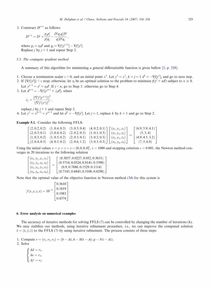
5.3. The conjugate gradient method
A summary of this algorithm for minimizing a general differentiable function is given bellow [3, p. 329].
1. Choose a termination scalar � > 0, and an initial point x1. Let y1 = x1, k = j = 1 d1 = �$f[y1], and go to next step.2. If k$f [yj]k < � stop; otherwise, let aj be an optimal solution to the problem to minimize f(yj + adj) subject to a P 0.
Let yj+1 = yj + ajdj. If j < n, go to Step 3. otherwise go to Step 4.
3. Let dj+1 = �$f [yj+1 + kjdj], where
kj ¼jjrf ½yjþ1�jj2
jjrf ðyjÞjj2;
replace j by j + 1 and repeat Step 2.4. Let y1 = xk+1 = yn+1 and let d1 = �$f[yj]. Let j = 1, replace k by k + 1 and go to Step 2.
Example 5.1. Consider the following FFLS:
ð2; 0:2; 0:2Þ ð1; 0:4; 0:3Þ ð3; 0:3; 0:4Þ ð4; 0:2; 0:1Þð2; 0:3; 0:1Þ ð3; 0:4; 0:2Þ ð2; 0:2; 0:3Þ ð1; 0:1; 0:3Þð1; 0:3; 0:2Þ ð1; 0:5; 0:2Þ ð2; 0:3; 0:1Þ ð3; 0:2; 0:3Þð2; 0:4; 0:5Þ ð4; 0:5; 0:2Þ ð2; 0:6; 1:2Þ ð3; 0:3; 0:3Þ
26643775ðx1; y1; z1Þðx2; y2; z2Þðx3; y3; z3Þðx4; y4; z4Þ
26643775 ¼
ð6:9; 5:9; 4:1Þð5; 3; 4Þ
ð4:9; 4:5; 3:2Þð7; 5; 6:8Þ
26643775:
Using the initial values x = y = z = s = [0,0,0,0]t, k = 1000 and stopping criterion � = 0.001, the Newton method con-verges in 20 iterations to the following solution
ðx1; y1; z1; s1Þðx2; y2; z2; s2Þðx3; y3; z3; s3Þðx4; y4; z4; s4Þ
26643775 ¼
ð0:3857; 0:0227; 0:052; 0:3631Þð0:5714; 0:0324; 0:8141; 0:5390Þð0:9; 0:7886; 0:1529; 0:1114Þð0:7143; 0:6845; 0:5108; 0:0298Þ
26643775:
Note that the optimal value of the objective function in Newton method (34) for this system is
f ðx; y; z; sÞ ¼ 10�9:
0:3610
0:1819
0:1983
0:4374
2666437775:
6. Error analysis on numerical examples
The accuracy of iterative methods for solving FFLS (7) can be controlled by changing the number of iterations (k).We may stabilize our methods, using iterative refinement procedure, i.e., we can improve the computed solution~x ¼ ðx; y; zÞ to the FFLS (7) by using iterative refinement. The process consists of three steps:
1. Compute r ¼ ðr1; r2; r3Þ ¼ ðb� Ax; h�Mx� Ay; g � Nx� AzÞ.2. Solve
Ad ¼ r1;
Ae ¼ r2;
Af ¼ r3:
8><>:

330 M. Dehghan et al. / Chaos, Solitons and Fractals 34 (2007) 316–336
3. Update ðx0; y0; z0Þ ¼ ðxþ d; y þ e; zþ f Þ.If there were no rounding errors in the computation of (r1, r2, r3), (d,e, f) and (x 0,y 0,z 0), then the exact solution to theFFLS, would be (x 0,y 0,z 0). For more information as to the accuracy and stability of stationary iterative methods, seethe excellent book [23] by Higham.
Now Consider the following FFLS,
Fig. 1.
ð4; 3; 2Þ ð3; 2; 3Þð5; 1; 4Þ ð6; 3; 1Þ
� � ex1ex2
� �¼ð17; 22; 30Þð28; 28; 39Þ
� �:
Employing our approach, its solution is
ex1ex2� �¼ð2; 1; 2Þð3; 2; 3Þ
� �:
We define 5 criteria for clarifying the amount of errors between the exact solution and our proposed solution. Note that
eA~x ¼ eb; iff ½eA�k½~x�k ¼ ½eb�k; where k 2 [0,1]. Thus we can employ this criterion for validation the results. LetALðkÞxLðkÞ ¼ bLðkÞ;
where AL(k), bL(k) and xL(k) be matrices which consisting of the lower bounds of k-cut of eA, eb and ~x. Similarly, AR(k),bR(k) and xR(k) denote the matrices including the upper bounds of k-cut of eA, eb and ~x respectively, which satisfy in thefollowing system
(a) The left and right errors respect to k, where L and R be linear functions. (b) Constrained with positivity of the solution.

TableThe re
max_e
12026.
Fig. 2.solutio
M. Dehghan et al. / Chaos, Solitons and Fractals 34 (2007) 316–336 331
ARðkÞxRðkÞ ¼ bRðkÞ:
Moreover suppose that ex� ; x*,L(k) and x*,R(k) be our determined solution, and the lower and upper bounds of its k-cut,respectively. With the above notations our criteria can be outlined as follows:
• max_error_left: The maximum error between x*,L(k) and xL(k), over k 2 [0,1].• max_error_right: The maximum error between x*,R(k) and xR(k), over k 2 [0,1].• average_error_left: The average error between x*,L(k) and xL(k), over all experiments.• average_error_right: The average error between x*,R(k) and xR(k), over all experiments.• average_error: The average between max_error_right and max_error_right.
2sults when L and R are linear functions
rror_left max_error_right average_error_left average_error_right average_error
0 204.16 138.84 8.66 147.50
(a) The left and right errors respect to k, where L be linear and R be nonlinear functions. (b) Constrained with positivity of then.

332 M. Dehghan et al. / Chaos, Solitons and Fractals 34 (2007) 316–336
In the following figures, with respect to k 2 [0,1] the error_left and error_right are represented. Also the criteriaamounts for linear functions L(x) = R(x) = 1 � x, are given in Fig. 1(a) and Table 2.
Note that the maximum errors, represented in Fig. 1(a), for the left and right shapes are revealed for k = 0.22 andk = 0.45 which are related to the following ill-posed matrices
Fig. 3.
AL ¼1:63 1:42
4:21 3:63
� �;
and
AR ¼5:10 4:65
7:20 6:55
� �
with the condition numbers of 580.33 and 1898.30, respectively. Moreover their solutions arexL ¼ ð7880;�9084Þ;xR ¼ ð140:23;�146; 60Þ;
which are not positive (Fig. 1(a)), while we applied our methods for finding positive solutions.In the next test, whenever both xL and xR are non-negative vectors, we register the results. By this constraint,
Fig. 1(b) presents the result of left and right errors.In another test, we set L(x) = 1 � x as a linear and RðxÞ ¼ 1
1þx2 a nonlinear function. The results of left and righterrors can be seen in Fig. 2(a) and (b). Also Fig. 3(a) and (b) shows the left and right errors for the case in whichLðxÞ ¼ 1
1þx, and RðxÞ ¼ 11þx2, respectively.
(a) The left and right errors respect to k, where L and R be nonlinear functions. (b) Constrained with positivity of the solution.
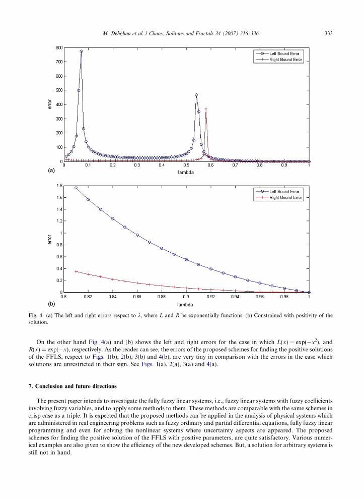
Fig. 4. (a) The left and right errors respect to k, where L and R be exponentially functions. (b) Constrained with positivity of thesolution.
M. Dehghan et al. / Chaos, Solitons and Fractals 34 (2007) 316–336 333
On the other hand Fig. 4(a) and (b) shows the left and right errors for the case in which L(x) = exp(�x2), andR(x) = exp(�x), respectively. As the reader can see, the errors of the proposed schemes for finding the positive solutionsof the FFLS, respect to Figs. 1(b), 2(b), 3(b) and 4(b), are very tiny in comparison with the errors in the case whichsolutions are unrestricted in their sign. See Figs. 1(a), 2(a), 3(a) and 4(a).
7. Conclusion and future directions
The present paper intends to investigate the fully fuzzy linear systems, i.e., fuzzy linear systems with fuzzy coefficientsinvolving fuzzy variables, and to apply some methods to them. These methods are comparable with the same schemes incrisp case as a triple. It is expected that the proposed methods can be applied in the analysis of physical systems whichare administered in real engineering problems such as fuzzy ordinary and partial differential equations, fully fuzzy linearprogramming and even for solving the nonlinear systems where uncertainty aspects are appeared. The proposedschemes for finding the positive solution of the FFLS with positive parameters, are quite satisfactory. Various numer-ical examples are also given to show the efficiency of the new developed schemes. But, a solution for arbitrary systems isstill not in hand.
334 M. Dehghan et al. / Chaos, Solitons and Fractals 34 (2007) 316–336
Acknowledgement
We would like to offer particular thanks to Mr. Ali Taghizadeh (Razi University, English Department, Kermanshah,Iran) for the language editing of this paper.
Appendix A. Fuzzy numbers and arithmetic operators
Fuzzy numbers are one way to describe the vagueness and lack of precision of data. They can be regarded as anextension of (crisp) real numbers. The concept of a fuzzy number was first used by Nahmias in the United Statesand by Dubois and Prade in France in the late 1970s, as follows:
Definition A.1. A fuzzy number eA is an upper semi-continuous, normal and convex fuzzy subset of the real line R suchthat leA : R7!½0; 1� where leAðxÞ is the membership function of eA, i.e., there exist x that leAðxÞ ¼ 1, andleAðkx1 þ ð1� kÞx2ÞP Minflex1
; lex2g, for k 2 [0,1].
Moreover a fuzzy number eA is called positive (negative), denoted by eA > 0 (eA < 0), if its membership function leAðxÞsatisfies leAðxÞ ¼ 0; 8x < 0 ð8x > 0Þ:
Definition A.2 (a-level set). The a-level set of a fuzzy set eA is defined as an ordinary set ½eA�a for which the degree of itsmembership function exceeds the level a:
½eA�a ¼ fxjleAðxÞP a; a 2 ½0; 1�g:
Definition A.3 (LR fuzzy numbers). A fuzzy number eA is said to be an LR fuzzy number if
leAðxÞ ¼ Lða�xa Þ; x 6 a; a > 0;
Rðx�ab Þ; x P a; b > 0;
(
where a is the mean value of eA and a and b are left and right spreads, respectively, and the function L(Æ) which is calledleft shape function satisfying:(1) L(x)=L(�x).(2) L(0)=1 and L(1)=0.(3) L(x) is non-increasing on [0,1).
Naturally, a right shape function R(Æ) is similarly defined as L(Æ).Using its mean value and left and right spreads, and shape functions, such a LR fuzzy number eA is symbolically
written as
eA ¼ ða; a; bÞLR:Clearly, eA ¼ ða; a; bÞLR is positive, if and only if, a � a > 0, (Since L(1) = 0).Also two LR fuzzy numbers eA ¼ ða; a; bÞLR and eB ¼ ðb; c; dÞLR are said to be equal, if and only if a = b, a = c and
b = d.On the other hand since each fuzzy number is a set, we can define its subset as follows:A LR fuzzy number eA ¼ ða; a; bÞLR is said to be a subset of the LR fuzzy number eB ¼ ðb; c; dÞLR, if and only if
a � a P b � c and a + b 6 b + d. Still there are other representations for fuzzy numbers, too (see e.g. [29]).
Definition A.4 (Extension Principle [32]). Let f : X! Y be a mapping from a set X to set Y. Then the extension prin-ciple allows you to define the fuzzy set eB in Y induced by the fuzzy set eA in X through f as follows:
eB ¼ fðy; leBðyÞÞjy ¼ f ðxÞ; x 2 Xg;with
leBðyÞ ¼ lf ðeAÞðyÞ ¼ sup
y¼f ðxÞleAðxÞ; f �1ðyÞ 6¼ /;
0; f �1ðyÞ ¼ /;
8<:
where f�1(y) is the inverse image of y.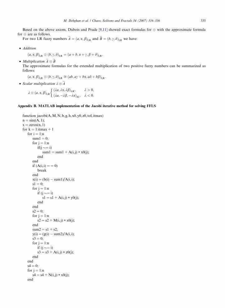
M. Dehghan et al. / Chaos, Solitons and Fractals 34 (2007) 316–336 335
Based on the above axiom, Dubois and Prade [9,11] showed exact formulas for � with the approximate formulafor � are as follows.
For two LR fuzzy numbers eA ¼ ða; a; bÞLR and eB ¼ ðb; c; dÞLR we have:
• Addition
ða; a; bÞLR � ðb; c; dÞLR ¼ ðaþ b; aþ c; bþ dÞLR:
• Multiplication eA � eBThe approximate formulas for the extended multiplication of two positive fuzzy numbers can be summarized asfollows:
ða; a; bÞLR � ðb; c; dÞLR ffi ðab; acþ ba; adþ bbÞLR:
• Scalar multiplication k� eA
k� ða; a; bÞLRðka; ka; kbÞLR; k > 0;
ðka;�kb;�kaÞRL; k < 0:
�
Appendix B. MATLAB implementation of the Jacobi iterative method for solving FFLS
function jacobi(A,M,N,b,g,h,x0,y0, z0, tol, itmax)n = size(A, 1);x = zeros(n,1)for k = 1:itmax + 1
for i = 1:nsum1 = 0;for j = 1:n
if(j = i)sum1 = sum1 + A(i, j) * x0(j);
endendif (A(i, i) = = 0)
breakendx(i) = (b(i) � sum1)/A(i, i);
s1 = 0;for j = 1:nif (j = i)s1 = s1 + A(i, j) * y0(j);
endends2 = 0;for j = 1:n
s2 = s2 + M(i, j) * x0(j);endsum2 = s1 + s2;y(i) = (g(i) � sum2)/A(i, i);
s3 = 0;for j = 1:nif (j = i)s3 = s3 + A(i, j) * z0(j);
endends4 = 0;for j = 1:n
s4 = s4 + N(i, j) * x0(j);end
336 M. Dehghan et al. / Chaos, Solitons and Fractals 34 (2007) 316–336
sum3 = s3 + s4;z(i) = (h(i) � sum3)/A(i, i);
endx0 = x;y0 = y;z0 = z;
endx = xy = yz = z
References
[1] Abbod MF, von Keyserlingk DG, Linkens DA, Mahfouf M. Survey of utilisation of fuzzy technology in medicine and healthcare.Fuzzy Sets Syst 2001;120:331–49.
[2] Avdelas G, Hadjidimos A. Optimum accelerated overrelaxation method in a special case. Math Comput 1981;36:183–7.[3] Bazaraa MS, Sherali HD, Shetty CM. Nonlinear programming, theory and algorithms. New York: John Wiley and Sons; 1993.[4] Buckley JJ, Qu Y. Solving systems of linear fuzzy equations. Fuzzy Sets Syst 1991;43:33–43.[5] Caldas M, Jafari S. h-Compact fuzzy topological spaces. Chaos, Solitons & Fractals 2005;25:229–32.[6] Datta BN. Numerical linear algebra and applications. California: Brooks/Cole Pub.; 1995.[7] Dehghan M, Hashemi B, Ghatee M. Computational methods for solving fully fuzzy linear systems. Appl Math Comput, in press.[8] DeMarr R. Nonnegative matrices with nonnegative inverses. Proc Amer Math Soc 1972;35:307–8.[9] Dubois D, Prade H. Operations on fuzzy numbers. Int J Syst Sci 1978;9:613–26.
[10] Dubois D, Prade H. Systems of linear fuzzy constraints. Fuzzy Sets Syst 1980;3:37–48.[11] Dubois D, Prade H. Fuzzy sets and systems: theory and applications. New York: Academic Press; 1980.[12] El Naschie MS. From experimental quantum optics to quantum gravity via a fuzzy Kahler manifold. Chaos, Solitons & Fractals
2005;25:969–77.[13] Evans DJ. The extrapolated modified Aitken iteration method for solving elliptic difference equations. Comput J 1963;6:193–201.[14] Friedman M, Ming M, Kandel A. Fuzzy linear systems. Fuzzy Sets Syst 1998;96:201–9.[15] Giachetti RE, Young RE. Analysis of the error in the standard approximation used for multiplication of triangular and
trapezoidal fuzzy numbers and the development of a new approximation. Fuzzy Sets Syst 1997;91:1–13.[16] Gvozdik AA. Solution of fuzzy equations. UDC 1985;518.9:60–7.[17] Hadjidimos A. Accelerated overrelaxation method. Math Comput 1978;32:149–57.[18] Hageman LA, Young DM. Applied iterative methods. New York: Academic Press; 1981.[19] Hansen E. Interval arithmetic in matrix computations, Part I. SIAM J Numer Anal 1965;2:308–20.[20] Hansen E. Interval arithmetic in matrix computations, Part II. SIAM J Numer Anal 1967;4:1–9.[21] Hansen ER. Interval forms of Newton’s method. Computing 1978;20:153–63.[22] Hansel E, Walster WG, Hansen ER, Walster GW. Global optimization using interval analysis. USA: Marcel Dekker; 2003.[23] Higham NJ. Accuracy and stability of numerical algorithms. Philadelphia: SIAM; 1996.[24] Kawaguchi MF, Da-Te T. A calculation method for solving fuzzy arithmetic equations with triangular norms. In: 2nd IEEE int
conf on fuzzy systems, San Francisco, USA, 1993.[25] Kreinovich V, Lakeyev AV, Rohn J, Kahl PT. Computational complexity and feasibility of data processing and interval
computations. Series: Appl Optimiz, 10. Springer; 1998.[26] Madalena Martins M. On an accelerated overrelaxation iterative method for linear systems with strictly diagonally dominant
matrix. Math Comput 1980;152:1269–73.[27] Missirils NM, Evans DJ. On the convergence of some generalized preconditioned iterative methods. SIAM J Numer Anal
1981;18:591–6.[28] Rao SS, Chen L. Numerical solution of fuzzy linear equations in engineering analysis. Int J Numer Methods Eng 1998;42:829–46.[29] Stefanini L, Sorini L, Letizia Guerra M. Simulation of fuzzy dynamical systems using the LU-representation of fuzzy numbers.
Chaos, Solitons & Fractals 2006;29:638–52.[30] Wagenknecht M, Hampel R, Schneider V. Computational aspects of fuzzy arithmetics based on Archimedean t-norms. Fuzzy Sets
Syst 2001;123:49–62.[31] Young DM. Iterative solution of large linear systems. New York: Academic Press; 1971.[32] Zadeh LA. Fuzzy sets. Inform Control 1965;8:338–53.[33] Zhang H, Liao X, Yu J. Fuzzy modeling and synchronization of hyperchaotic systems. Chaos, Solitons & Fractals
2005;26:835–43.[34] Zhao R, Govind R. Solutions of algebraic equations involving generalized fuzzy numbers. Inform Sci 1991;56:199–243.