Controlled switching in Kalman filtering and iterative learning ...
Upload
khangminh22Category
view
0download
0
Mathematics 19-61
© 1999 by CRC Press LLC
With y(x; ε) = y0(u, v) + εy1(u, v) + ε2y2(u, v) + L we have terms
Then y0(u, v) = A(u) + B(u)e–v and so the second equation becomes ∂2y1/∂v2 + ∂y1/∂v = 2 – A′(u) +B′(u)e–v, with the solution y1(u, v) = [2 – A′(u)]v + vB′(u)e–v + D(u) + E(u)e–v. Here A, B, D and E arestill arbitrary. Now the solvability condition — “higher order terms must vanish no slower (as ε → 0)than the previous term” (Kevorkian and Cole, 1981) — is used. For y1 to vanish no slower than y0 wemust have 2 – A′(u) = 0 and B′(u) = 0. If this were not true the terms in y1 would be larger than thosein y0 (v @ 1). Thus y0(u, v) = (2u + A0) + B0e–v, or in the original variables y(x; ε) ≈ (2x + A0) + B0e–x/ε
and matching to both boundary conditions gives y(x; ε) ≈ 2x – (1 – e–x/ε).
Boundary Layer Method
The boundary layer method is applicable to regions in which the solution is rapidly varying. See thereferences at the end of the chapter for detailed discussion.
Iterative Methods
Taylor Series
If it is known that the solution of a differential equation has a power series in the independent variable(t), then we may proceed from the initial data (the easiest problem) to compute the Taylor series bydifferentiation.
Example 19.7.3. Consider the equation (d2x/dt) = – x – x2, x(0) = 1, x′(0) = 1. From the differentialequation, x″(0) = –2, and, since x- = –x′ –2xx′, x-(0) = –1 –2 = –3, so the four term approximation forx(t) ≈ 1 + t – (2t2/2!) – (3t3/3!) = 1 + t – t2 – t3/2. An estimate for the error at t = t1, (see a discussionof series methods in any calculus text) is not greater than |d4x/dt4|max[(t1)4/4!], 0 ≤ t ≤ t1.
Picard’s Method
If the vector differential equation x′ = f(t, x), x(0) given, is to be approximated by Picard iteration, webegin with an initial guess x0 = x(0) and calculate iteratively = f(t, xi–1).
Example 19.7.4. Consider the equation x′ = x + y2, y′ = y – x3, x(0) = 1, y(0) = 2. With x0 = 1, y0 = 2,= 5, = 1, so x1 = 5t + 1, y1 = t + 2, since xi(0) = 1, yi(0) = 2 for i ≥ 0. To continue, use = xi
+ = yi – A modification is the utilization of the first calculated term immediately in thesecond equation. Thus, the calculated value of x1 = 5t + 1, when used in the second equation, gives = y0 – (5t + 1)3 = 2 – (125t3 + 75t2 + 15t + 1), so y1 = 2t – (125t4/4) – 25t3 – (15t2/2) – t + 2. Continuewith the iteration = xi + = yi – (xi+1)3.
Another variation would be = xi+1 + (yi)3, = yi+1 – (xi+1)3.
ε ∂∂ ε
∂∂
∂∂ ε
∂∂u v
yu v
y+
+ +
=1 12
2
Oy
v
y
vu
Oy
v
y
v
y
u v
y
u
Oy
v
y
v
y
u v
y
u
y
u
ε∂∂
∂∂
ε∂∂
∂∂
∂∂ ∂
∂∂
ε∂∂
∂∂
∂∂ ∂
∂∂
∂∂
−( ) + = ( )
( ) + = − −
( ) + = − − −
12
02
0
02
12
12
0 0
12
22
22
1 12
02
0
2 2
2
:
:
:
actually ODEs with parameter
M
′xi
′x1 ′y1 ′+xi 1
yi2 , ′+yi 1 xi
3.′y1
′+xi 1 yi3, ′+yi 1
′+xi 1 ′+yi 1

19-62 Section 19
© 1999 by CRC Press LLC
References
Ames, W. F. 1965. Nonlinear Partial Differential Equations in Science and Engineering, Volume I.Academic Press, Boston, MA.
Ames, W. F. 1968. Nonlinear Ordinary Differential Equations in Transport Processes. Academic Press,Boston, MA.
Ames, W. F. 1972. Nonlinear Partial Differential Equations in Science and Engineering, Volume II.Academic Press, Boston, MA.
Kevorkian, J. and Cole, J. D. 1981. Perturbation Methods in Applied Mathematics, Springer, New York.Miklin, S. G. and Smolitskiy, K. L. 1967. Approximate Methods for Solutions of Differential and Integral
Equations. Elsevier, New York.Nayfeh, A. H. 1973. Perturbation Methods. John Wiley & Sons, New York.Zwillinger, D. 1992. Handbook of Differential Equations, 2nd ed. Academic Press, Boston, MA.
19.8 Integral Transforms
William F. Ames
All of the integral transforms are special cases of the equation g(s) = K(s, t)f(t)d t, in which g(s) issaid to be the transform of f(t), and K(s, t) is called the kernel of the transform. Table 19.8.1 shows themore important kernels and the corresponding intervals (a, b).
Details for the first three transforms listed in Table 19.8.1 are given here. The details for the otherare found in the literature.
Laplace Transform
The Laplace transform of f(t) is g(s) = e–st f(t) dt. It may be thought of as transforming one class offunctions into another. The advantage in the operation is that under certain circumstances it replacescomplicated functions by simpler ones. The notation L[f(t)] = g(s) is called the direct transform andL–1[g(s)] = f(t) is called the inverse transform. Both the direct and inverse transforms are tabulated formany often-occurring functions. In general L–1[g(s)] = (1/2 πi) estg(s) ds, and to evaluate this integralrequires a knowledge of complex variables, the theory of residues, and contour integration.
Properties of the Laplace Transform
Let L[f(t)] = g(s), L–1[g(s)] = f(t).
1. The Laplace transform may be applied to a function f(t) if f(t) is continuous or piecewisecontinuous; if tn|f(t)| is finite for all t, t → 0, n < 1; and if e–at|f(t)| is finite as t → ∞ for somevalue of a, a > 0.
2. L and L–1 are unique.3. L[af(t) + bh(t)] = aL[f(t)] + bL[h(t)] (linearity).4. L[eatf(t)] = g(s – a) (shift theorem).5. L[(–t)kf(t)] = dkg/dsk; k a positive integer.
Example 19.8.1. L[sin a t] = e–st sin a t d t = a/(s2 + a2), s > 0. By property 5,
∫ ab
∫ ∞0
∫ − ∞+ ∞
αα
ii
∫ ∞0
02 2
2∞−∫ = [ ] =
+e t at dt L t at
as
s ast sin sin

Mathematics 19-63
© 1999 by CRC Press LLC
6.
In this property it is apparent that the initial data are automatically brought into the computation.
Example 19.8.2. Solve y″ + y = et, y(0) = 1, y′(0) = 1. Now L[y″] = s2L[y] – sy(0) – y′(0) = s2L[y] –s – 1. Thus, using the linear property of the transform (property 3), s2L[y] + L[y] – s – 1 = L[et] = 1/(s– 1). Therefore, L[y] =s2/[(s – 1)(s2 + 1)].
With the notations Γ(n + 1) = xne–x dx (gamma function) and Jn(t) the Bessel function of the firstkind of order n, a short table of Laplace transforms is given in Table 19.8.2.
7.
Example 19.8.3. Find f(t) if L[f(t)] = (1/s2)[1/(s2 – a2)]. L[1/a sinh a t] = 1/(s2 – a2). Therefore, f(t) =[ sinh a t d t]d t = 1/a2[(sinh a t)/a – t].
Example 19.8.4. L[(sin a t)/t] = L[sin a t)d s = [a d s/(s2 + a2)] = cot–1(s/a).
9. The unit step function u(t – a) = 0 for t < a and 1 for t > a. L[u(t – a) = e–as/s.10. The unit impulse function is δ(a) = u′(t – a) = 1 at t = a and 0 elsewhere. L[u′(t – a) = e–as.11. L–1[e–asg(s)] = f(t – a)u(t – a) (second shift theorem).12. If f(t) is periodic of period b — that is, f(t + b) = f(t) — then L[f(t)] = [1/(1 – e–bs)] × e–stf(t) dt.
Example 19.8.5. The equation ∂2y/(∂t∂x) + ∂y/∂t + ∂y/∂x = 0 with (∂y/∂x)(0, x) = y(0, x) = 0 and y(t,0) + (∂y/∂t)(t, 0) = δ(0) (see property 10) is solved by using the Laplace transform of y with respect tot. With g(s, x) = e–sty(t, x) dt, the transformed equation becomes
Table 19.8.1 Kernels and Intervals of Various Integral Transforms
Name of Transform (a, b) K(s, t)
Laplace (0, ∞) e–st
Fourier (–∞, ∞)
Fourier cosine (0, ∞)
Fourier sine (0, ∞)
Mellin (0, ∞) ts–1
Hankel (0, ∞) tJv(st), v ≥
1
2πe ist−
2
πcos st
2
πsin st
− 12
L f t sL f t f
L f t s L f t sf f
L f t s L f t s f sf fn n n n n
′( )[ ] = ( )[ ] − ( )
′′( )[ ] = ( )[ ] − ( ) − ′( )
( )[ ] = ( )[ ] − ( ) − − ( ) − ( )( ) − −( ) −( )
0
0 0
0 0 0
2
1 2 1
M
L
∫ ∞0
L f t dt L f t f t dta
t
s sa∫ ∫( )
= ( )[ ] + ( )1 10
.
∫ 0t ∫ 0
1ta
Lf t
tg s ds L
f t
tg s ds
sk
s s
k
k( )
= ( ) ( )
= ( )( )∞ ∞ ∞
∫ ∫ ∫; K124 34
integrals
∫ ∞s ∫ ∞
s
∫ 0b
∫ ∞0

19-64 Section 19
© 1999 by CRC Press LLC
or
The second (boundary) condition gives g(s, 0) + sg(s, 0) – y(0, 0) = 1 or g(s, 0) = 1/(1 + s). A solutionof the preceding ordinary differential equation consistent with this condition is g(s, x) = [1/(s + 1)]e–sx/(s+1).Inversion of this transform gives y(t, x) = e–(t+x)I0 where I0 is the zero-order Bessel function ofan imaginary argument.
Convolution Integral
The convolution integral (faltung) of two functions f(t), r(t) is x(t) = f(t)* r(t) = f(τ)r(t – τ) d τ.
Example 19.8.6. t * sin t = τ sin(t – τ) d τ = t – sin t.
13. L[f(t)]L[h(t)] = L[f(t) * h(t)].
Fourier Transform
The Fourier transform is given by F[f(t)] = f(t)e–ist d t = g(s) and its inverse by F–1[g(s)]= g(s)eist d t = f(t). In brief, the condition for the Fourier transform to exist is that |f(t)|d t < ∞, although certain functions may have a Fourier transform even if this is violated.
Table 19.8.2 Some Laplace Transforms
f(t) g(s) f(t) g(s)
1 e–at(1 – a t)
tn, n is a + integer
tn, n ≠ a + integer
cos a t cos a t cosh a t
sin a t
cosh a t
sinh a t
e–at J0(a t)
e–bt cos a t
e–bt sin a t
1
s
s
s a+( )2
n
sn
!+1
t at
a
sin
2
s
s a2 2 2+( )
Γ n
sn
+( )+
11
1
2 2aat atsin sinh
s
s a4 44+
s
s a2 2+s
s a
3
4 44+a
s a2 2+1
2aat atsinh sin+( ) s
s a
2
4 4−s
s a2 2−12 cosh cosat at+( ) s
s a
3
4 4−a
s a2 2−sin at
ttan −1 a
s
1
s a+1
2 2s a+
s b
s b a
++( ) +2 2
n
a
J at
tnn ( ) 1
2 2s a sn
+ +
a
s b a+( ) +2 2 J at0 2( ) 1
se a s− /
sg
x
y
xx sg y x
g
x
∂∂
∂∂
∂∂
− ( ) + − ( ) + =0 0 0, ,
sg
xsg
y
xx y x+( ) + = ( ) + ( ) =1 0 0 0
∂∂
∂∂
, ,
( / ),2 tx
∫ 0t
∫ 0t
( / )1 2π ∫ −∞∞
( / )1 2π ∫ −∞∞ ∫ −∞
∞

Mathematics 19-65
© 1999 by CRC Press LLC
Example 19.8.7. The function f(t) = 1 for – a ≤ t ≤ a and = 0 elsewhere has
Properties of the Fourier Transform
Let F[f(t)] = g(s); F–1[g(s)] = f(t).
1. F[f(n)(t)] = (i s)n F[f(t)]2. F[af(t) + bh(t)] = aF[f(t)] + bF[h(t)]3. F[f(–t)] = g(–s)4. F[f(at)] = 1/a g(s/a), a > 05. F[e–iwtf(t)] = g(s + w)6. F[f(t + t1)] = g(s)7. F[f(t)] = G(i s) + G(–i s) if f(t) = f(–t)(f(t) even)
F[f(t)] = G(i s) – G(–i s) if f(t) = –f(–t)(f odd)
where G(s) = L[f(t)]. This result allows the use of the Laplace transform tables to obtain the Fouriertransforms.
Example 19.8.8. Find F[e–a|t|] by property 7. The term e–a|t| is even. So L[e–at] = 1/(s + a). Therefore,F[e–a|t|] = 1/(i s + a) + 1/(–i s + a) = 2a/(s2 + a2).
Fourier Cosine Transform
The Fourier cosine transform is given by Fc[f(t)] = g(s) = f(t) cos s t d t and its inverse by[g(s)] = f(t) = g(s) cos s t d s. The Fourier sine transform Fs is obtainable by replacing
the cosine by the sine in the above integrals.
Example 19.8.9. Fc[f(t)], f(t) = 1 for 0 < t < a and 0 for a < t < ∞. Fc [f(t)] = cos s t d t =(sin a s)/s.
Properties of the Fourier Cosine Transform
Fc[f(t)] = g(s).
1. Fc[af(t) + bh(t)] = aFc[f(t)] + bFc[h(t)]2. Fc[f(at)] = (1/a) g (s/a)3. Fc[f(at) cos bt] = 1/2a [g ((s + b)/a) + g((s – b)/a)], a, b > 04. Fc[t2nf(t)] = (– 1)n(d2ng)/(d s2n)5. Fc[t2n+1f(t)] = (– 1)n(d2n+1)/(d s2n+1) Fs[f(t)]
Table 19.8.3 presents some Fourier cosine transforms.
Example 19.8.10. The temperature θ in the semiinfinite rod 0 ≤ x < ∞ is determined by the differentialequation ∂θ/∂t = k(∂2θ/∂x2) and the condition θ = 0 when t = 0, x ≥ 0; ∂θ/∂x = –µ = constant when x =0, t > 0. By using the Fourier cosine transform, a solution may be found as θ(x, t) = (2µ/π) (cos px/p)(1 – e–kp2t) d p.
References
Churchill, R. V. 1958. Operational Mathematics. McGraw-Hill, New York.Ditkin, B. A. and Proodnikav, A. P. 1965. Handbook of Operational Mathematics (in Russian). Nauka,
Moscow.Doetsch, G. 1950–1956. Handbuch der Laplace Transformation, vols. I-IV (in German). Birkhauser,
Basel.
F f t e dt e dt e dt st dtsa
sa
aist
aist
aist
a
( )[ ] = = + = =−
− −∫ ∫ ∫ ∫0 0 02
2cos
sin
eist1
( / )2 0π ∫ ∞
Fc−1 ( / )2 0π ∫ ∞
( / )2 0π ∫ a
( / )2 π
∫ ∞0

19-66 Section 19
© 1999 by CRC Press LLC
Nixon, F. E. 1960. Handbook of Laplace Transforms. Prentice-Hall, Englewood Cliffs, NJ.Sneddon, I. 1951. Fourier Transforms. McGraw-Hill, New York.Widder, D. 1946. The Laplace Transform, Princeton University Press, Princeton, NJ.
Further Information
The references citing G. Doetsch, Handbuch der Laplace Transformation, vols. I-IV, Birkhauser, Basel,1950–1956 (in German) and B. A. Ditkin and A. P. Prodnikav, Handbook of Operational Math-ematics, Moscow, 1965 (in Russian) are the most extensive tables known. The latter reference is485 pages.
Table 19.8.3 Fourier Cosine Transforms
f(t)
t–1/2 π1/2(s)–1/2
π1/2(s)–1/2 [cos a s – sin a s]
(t2 + a2)–1
e–at, a > 0
a > 0
a > 0
g s( )2 π
t t
t t
t
0 1
2 1 2
0 2
< <− < <
< < ∞
12 1 22s
s scos cos− −[ ]
0 01 2
< <−( ) < < ∞
−t a
t a a t
12
1πa e as− −
a
s a2 2+
e at− 2
, 12
1 2 1 2 42
π a e s a− − /
sin at
t
ππ
2
4
0
s a
s a
s a
<=>

Mathematics 19-67
© 1999 by CRC Press LLC
19.9 Calculus of Variations
William F. Ames
The basic problem in the calculus of variations is to determine a function such that a certain functional,often an integral involving that function and certain of its derivatives, takes on maximum or minimumvalues. As an example, find the function y(x) such that y(x1) = y1, y(x2) = y2 and the integral (functional)I = 2π y[1 + y′)2]1/2 d x is a minimum. A second example concerns the transverse deformation u(x,t) of a beam. The energy functional I = [1/2 ρ (∂u/∂t)2 – 1/2 EI (∂2u/∂x2)2 + fu] d x d t is to beminimized.
The Euler Equation
The elementary part of the theory is concerned with a necessary condition (generally in the form of adifferential equation with boundary conditions) that the required function must satisfy. To show math-ematically that the function obtained actually maximizes (or minimizes) the integral is much moredifficult than the corresponding problems of the differential calculus.
The simplest case is to determine a function y(x) that makes the integral I = F(x, y, y′) dx stationaryand that satisfies the prescribed end conditions y(x1) = y1 and y(x2) = y2. Here we suppose F has continuoussecond partial derivatives with respect to x, y, and y′ = dy/dx. If y(x) is such a function, then it mustsatisfy the Euler equation (d/dx)(∂F/∂y′) – (∂F/∂y) = 0, which is the required necessary condition. Theindicated partial derivatives have been formed by treating x, y, and y′ as independent variables. Expandingthe equation, the equivalent form Fy′y′y″ + Fy′yy′ + (Fy′x – Fy) = 0 is found. This is second order in yunless Fy′y′ = (∂2F)/[(∂y′)2] = 0. An alternative form 1/y′[d/dx(F – (∂F/∂y′)(dy/dx)) – (∂F/∂x)] = 0 isuseful. Clearly, if F does not involve x explicitly [(∂F/∂x) = 0] a first integral of Euler’s equation is F– y′(∂F/∂y′) = c. If F does not involve y explicitly [(∂F/∂y) = 0] a first integral is (∂F/∂y′) = c.
The Euler equation for I = 2π y[1 + (y′)2]1/2 dx, y(x1) = y1, y(x2) = y2 is (d/dx)[yy′/[1 + (y′)2]1/2] –[1 + (y′)2]1/2 = 0 or after reduction yy″ – (y′)2 – 1 = 0. The solution is y = c1 cosh(x/c1 + c2), where c1
and c2 are integration constants. Thus the required minimal surface, if it exists, must be obtained byrevolving a catenary. Can c1 and c2 be chosen so that the solution passes through the assigned points?The answer is found in the solution of a transcendental equation that has two, one, or no solutions,depending on the prescribed values of y1 and y2.
The Variation
If F = F(x, y, y′), with x independent and y = y(x), then the first variation δF of F is defined to be δF= (∂F/∂x) δy + (∂F/∂y) δy′ and δy′ = δ (dy/dx) = (d/dx) (δy) — that is, they commute. Note that the firstvariation, δF, of a functional is a first-order change from curve to curve, whereas the differential of afunction is a first-order approximation to the change in that function along a particular curve. The lawsof δ are as follows: δ(c1F + c2G) = c1δF + c2δG; δ(FG) = FδG + GδF; δ(F/G) = (GδF – FδG)/G2; if xis an independent variable, δx = 0; if u = u(x, y); (∂/∂x)(δu) = δ(∂u/∂x), (∂/∂y) (δu) = δ(∂u/∂y).
A necessary condition that the integral I = F(x, y, y′) dx be stationary is that its (first) variationvanish — that is, δI = δ F(x, y, y′) dx = 0. Carrying out the variation and integrating by parts yieldsof δI = [(∂F/∂y) – (d/dx)(∂F/∂y′)] δy dx + [(∂F/∂y′) = 0. The arbitrary nature of δy means thesquare bracket must vanish and the last term constitutes the natural boundary conditions.
Example. The Euler equation of F(x, y, y′, y″) dx is (d2/dx2)(∂F/∂y″) – (d/dx)(∂F/∂y′) + (∂F/∂y) =0, with natural boundary conditions {[(d/dx)(∂F/∂y″) – (∂F/∂y′)] = 0 and (∂F/∂y″) = 0. TheEuler equation of F(x, y, u, ux, uy, uxx, uxy, uyy) dx dy is (∂2/∂x2)(∂F/∂uxx) + (∂2/∂x∂y)(∂F/uxy) +(∂2/∂y2)(∂F/∂uyy) – (∂/∂x)(∂F/∂ux) – (∂/∂y)(∂F/∂uy) + (∂F/∂u), and the natural boundary conditions are
∫ xx
1
2
∫ ∫tt L
1
20
∫ xx
1
2
∫ xx
1
2
∫ xx
1
2
∫ xx
1
2
∫ xx
1
2 ∂y xx]1
2
∫ xx
1
2
δy xx}1
2 δ ′y xx|1
2
∫ ∫xx
yy
1
2
1
2

19-68 Section 19
© 1999 by CRC Press LLC
In the more general case of I = F(x, y, u, v, ux, uy, vx, vy) dx dy, the condition δI = 0 gives rise tothe two Euler equations (∂/∂x)(∂F/∂ux) + (∂/∂y)(∂F/∂uy) – (∂F/∂u) = 0 and (∂/∂x)(∂F/∂vx) + (∂/∂y)(∂F/∂vy)– (∂F/∂v) = 0. These are two PDEs in u and v that are linear or quasi-linear in u and v. The Euler equationfor I = dx dy dz, from δI = 0, is Laplace’s equation uxx + uyy + uzz = 0.
Variational problems are easily derived from the differential equation and associated boundary con-ditions by multiplying by the variation and integrating the appropriate number of times. To illustrate,let F(x), ρ(x), p(x), and w be the tension, the linear mass density, the natural load, and (constant) angularvelocity of a rotating string of length L. The equation of motion is (d/dx)[F (dy/dx)] + ρw2y + p = 0. Toformulate a corresponding variational problem, multiply all terms by a variation δy and integrate over(0, L) to obtain
The second and third integrals are the variations of 1/2 ρw2y2 and py, respectively. To treat the firstintegral, integrate by parts to obtain
So the variation formulation is
The last term represents the natural boundary conditions. The term 1/2 ρw2y2 is the kinetic energy perunit length, the term –py is the potential energy per unit length due to the radial force p(x), and the term1/2 F(dy/dx)2 is a first approximation to the potential energy per unit length due to the tension F(x) inthe string. Thus the integral is often called the energy integral.
Constraints
The variations in some cases cannot be arbitrarily assigned because of one or more auxiliary conditionsthat are usually called constraints. A typical case is the functional F(x, u, v, ux, vx) dx with a constraintφ(u, v) = 0 relating u and v. If the variations of u and v (δu and δv) vanish at the end points, then thevariation of the integral becomes
∂∂
∂∂
∂∂
∂∂
∂∂
δ ∂∂
δ
∂∂
∂∂
∂∂
∂∂
∂
x
F
u y
F
u
F
uu
F
uu
y
F
u x
F
u
xx xy xx
x
xxx
x
x
yy xy
+
−
=
=
+
−
1
2
1
2
0 0,
FF
uu
F
uu
yy
y
yyy
y
y
∂δ ∂
∂δ
=
=
1
2
1
2
0 0,
∫ ∫ R
∫ ∫ ∫ + +R x y zu u u( )2 2 2
0 0
2
00
L L Ld
dxF
dy
dxy dx w y y dx p y dx∫ ∫ ∫
+ + =δ ρ δ δ
Fdy
dxy F
dy
dx
dy
dxdx F
dy
dxy F
dy
dxdx
L L L L
δ δ δ δ
− =
−
=∫ ∫
0 0 0 0
212
0
δ ρ δ0
2 22
0
12
12
0L L
w y py Fdy
dxdx F
dy
dxy∫ + −
+
=
∫ xx
1
2
∂∂
∂∂
δ ∂∂
∂∂
δF
u
d
dx
F
uu
F
v
d
dx
F
vv dx
x xx
x
−
+ −
=∫
1
2
0

Mathematics 19-69
© 1999 by CRC Press LLC
The variation of the constraint φ(u, v) = 0, φuδu + φvδv = 0 means that the variations cannot both beassigned arbitrarily inside (x1, x2), so their coefficients need not vanish separately. Multiply φuδu + φvδv= 0 by a Lagrange multiplier λ (may be a function of x) and integrate to find (λφuδu + λφvδv) dx =0. Adding this to the previous result yields
which must hold for any λ. Assign λ so the first square bracket vanishes. Then δv can be assigned tovanish inside (x1, x2) so the two systems
plus the constraint φ(u, v) = 0 are three equations for u, v and λ.
References
Gelfand, I. M. and Fomin, S. V. 1963. Calculus of Variations. Prentice Hall, Englewood Cliffs, NJ.Lanczos, C. 1949. The Variational Principles of Mechanics. Univ. of Toronto Press, Toronto.Schechter, R. S. 1967. The Variational Method in Engineering, McGraw-Hill, New York.Vujanovic, B. D. and Jones, S. E. 1989. Variational Methods in Nonconservative Phenomena. Academic
Press, New York.Weinstock, R. 1952. Calculus of Variations, with Applications to Physics and Engineering. McGraw-
Hill, New York.
∫ xx
1
2
∂∂
∂∂
λφ δ ∂∂
∂∂
λφ δF
u
d
dx
F
uu
F
v
d
dx
F
vv dx
xu
xv
x
x
−
+
+ −
+
=∫
1
2
0
d
dx
F
u
F
u
d
dx
F
v
F
vxu
xv
∂∂
∂∂
λφ ∂∂
∂∂
λφ
− − =
− − =0 0,
19-70 Section 19
© 1999 by CRC Press LLC
19.10 Optimization Methods
George Cain
Linear Programming
Let A be an m × n matrix, b a column vector with m components, and c a column vector with ncomponents. Suppose m < n, and assume the rank of A is m. The standard linear programming problemis to find, among all nonnegative solutions of Ax = b, one that minimizes
This problem is called a linear program. Each solution of the system Ax = b is called a feasible solution,and the feasible set is the collection of all feasible solutions. The function cTx = c1x1 + c2x2 + L + cnxn
is the cost function, or the objective function. A solution to the linear program is called an optimalfeasible solution.
Let B be an m × n submatrix of A made up of m linearly independent columns of A, and let C bethe m × (n – m) matrix made up of the remaining columns of A. Let xB be the vector consisting of thecomponents of x corresponding to the columns of A that make up B, and let xC be the vector of theremaining components of x, that is, the components of x that correspond to the columns of C. Then theequation Ax = b may be written BxB + CxC = b. A solution of BxB = b together with xC = 0 gives asolution x of the system Ax = b. Such a solution is called a basic solution, and if it is, in addition,nonnegative, it is a basic feasible solution. If it is also optimal, it is an optimal basic feasible solution.The components of a basic solution are called basic variables.
The Fundamental Theorem of Linear Programming says that if there is a feasible solution, there is abasic feasible solution, and if there is an optimal feasible solution, there is an optimal basic feasiblesolution. The linear programming problem is thus reduced to searching among the set of basic solutionsfor an optimal solution. This set is, of course, finite, containing as many as n!/[m!(n – m)!] points. Inpractice, this will be a very large number, making it imperative that one use some efficient searchprocedure in seeking an optimal solution. The most important of such procedures is the simplex method,details of which may be found in the references.
The problem of finding a solution of Ax ≤ b that minimizes cTx can be reduced to the standard problemby appending to the vector x an additional m nonnegative components, called slack variables. The vectorx is replaced by z, where zT = [x1,x2…xn s1,s2…xm], and the matrix A is replaced by B = [A I ], where Iis the m × m identity matrix. The equation Ax = b is thus replaced by Bz = Ax + s = b, where sT =[s1,s2,…,sm]. Similarly, if inequalities are reversed so that we have Ax ≤ b, we simply append –s to thevector x. In this case, the additional variables are called surplus variables.
Associated with every linear programming problem is a corresponding dual problem. If the primalproblem is to minimize cTx subject to Ax ≥ b, and x ≥ 0, the corresponding dual problem is to maximizeyTb subject to tTA ≤ cT. If either the primal problem or the dual problem has an optimal solution, soalso does the other. Moreover, if xp is an optimal solution for the primal problem and yd is an optimalsolution for the corresponding dual problem cTxp =
Unconstrained Nonlinear Programming
The problem of minimizing or maximizing a sufficiently smooth nonlinear function f(x) of n variables,xT = [x1,x2…xn], with no restrictions on x is essentially an ordinary problem in calculus. At a minimizeror maximizer x*, it must be true that the gradient of f vanishes:
c xT = + + +c x c x c xn n1 1 2 2 L
y bdT .
∇ ( ) =f x* 0

Mathematics 19-71
© 1999 by CRC Press LLC
Thus x* will be in the set of all solutions of this system of n generally nonlinear equations. The solutionof the system can be, of course, a nontrivial undertaking. There are many recipes for solving systemsof nonlinear equations. A method specifically designed for minimizing f is the method of steepest descent.It is an old and honorable algorithm, and the one on which most other more complicated algorithms forunconstrained optimization are based. The method is based on the fact that at any point x, the directionof maximum decrease of f is in the direction of –∇ f(x). The algorithm searches in this direction for aminimum, recomputes ∇ f(x) at this point, and continues iteratively. Explicitly:
1. Choose an initial point x0.2. Assume xk has been computed; then compute yk = ∇ f(xk), and let tk ≥ 0 be a local minimum of
g(t) = f(xk – tyk). Then xk+1 = xk – tkyk.3. Replace k by k + 1, and repeat step 2 until tk is small enough.
Under reasonably general conditions, the sequence (xk) converges to a minimum of f.
Constrained Nonlinear Programming
The problem of finding the maximum or minimum of a function f(x) of n variables, subject to theconstraints
is made into an unconstrained problem by introducing the new function L(x):
where zT = [λ1,λ2,…,λm] is the vector of Lagrange multipliers. Now the requirement that ∇ L(x) = 0,together with the constraints a(x) = b, give a system of n + m equations
for the n + m unknowns x1, x2…, xn, λ1λ2…, λm that must be satisfied by the minimizer (or maximizer) x.The problem of inequality constraints is significantly more complicated in the nonlinear case than in
the linear case. Consider the problem of minimizing f(x) subject to m equality constraints a(x) = b, andp inequality constraints c(x) ≤ d [thus a(x) and b are vectors of m components, and c(x) and d arevectors of p components.] A point x* that satisfies the constraints is a regular point if the collection
where
a x b( ) =
( )( )
( )
=
=
a x x x
a x x x
a x x x
b
b
b
n
n
m n m
1 1 2
2 1 2
1 2
1, , ,
, , ,
, , ,
K
K
M
K
M
L fx x z a x( ) = ( ) + ( )T
∇ ( ) + ∇ ( ) =
( ) =
f x z a x
a x b
T 0
∇ ( ) ∇ ( ) ∇ ( ){ } ∪ ∇ ( ) ∈{ }a a a c j Jm j1 2x x x x* * * *, , , :K
J j c dj j= ( ) ={ }: *x

19-72 Section 19
© 1999 by CRC Press LLC
is linearly independent. If x* is a local minimum for the constrained problem and if it is a regular point,there is a vector z with m components and a vector w ≥ 0 with p components such that
These are the Kuhn-Tucker conditions. Note that in order to solve these equations, one needs to knowfor which j it is true that cj(x*) = 0. (Such a constraint is said to be active.)
References
Luenberger, D. C. 1984. Linear and Nonlinear Programming, 2nd ed. Addison-Wesley, Reading, MA.Peressini, A. L. Sullivan, F. E., and Uhl, J. J., Jr. 1988. The Mathematics of Nonlinear Programming.
Springer-Verlag, New York.
∇ ( ) + ∇ ( ) + ∇ ( ) =
( ) −( ) =
f x z a x w c x
w c x d
* * *
*
T T
T
0
0

Mathematics 19-73
© 1999 by CRC Press LLC
19.11 Engineering Statistics
Y. L. Tong
Introduction
In most engineering experiments, the outcomes (and hence the observed data) appear in a random andon deterministic fashion. For example, the operating time of a system before failure, the tensile strengthof a certain type of material, and the number of defective items in a batch of items produced are allsubject to random variations from one experiment to another. In engineering statistics, we apply thetheory and methods of statistics to develop procedures for summarizing the data and making statisticalinferences, thus obtaining useful information with the presence of randomness and uncertainty.
Elementary Probability
Random Variables and Probability Distributions
Intuitively speaking, a random variable (denoted by X, Y, Z, etc.) takes a numerical value that dependson the outcome of the experiment. Since the outcome of an experiment is subject to random variation,the resulting numerical value is also random. In order to provide a stochastic model for describing theprobability distribution of a random variable X, we generally classify random variables into two groups:the discrete type and the continuous type. The discrete random variables are those which, technicallyspeaking, take a finite number or a countably infinite number of possible numerical values. (In mostengineering applications they take nonnegative integer values.) Continuous random variables involveoutcome variables such as time, length or distance, area, and volume. We specify a function f(x), calledthe probability density function (p.d.f.) of a random variable X, such that the random variable X takesa value in a set A (or real numbers) as given by
(9.11.1)
By letting A be the set of all values that are less than or equal to a fixed number t, i.e., A = (–∞,t), theprobability function P[X ≤ t], denoted by F(t), is called the distribution function of X. We note that, bycalculus, if X is a continuous random variable and if F(x) is differentiable, then f(x) = F(x).
Expectations
In many applications the “payoff” or “reward” of an experiment with a numerical outcome X is a specificfunction of X (u(X), say). Since X is a random variable, u(X) is also a random variable. We define theexpected value of u(X) by
(9.11.12)
provided of course, that, the sum or the integral exists. In particular, if u(x) = x, the EX ≡ µ is calledthe mean of X (of the distribution) and E(X – µ)2 ≡ σ2 is called the variance of X (of the distribution).The mean is a measurement of the central tendency, and the variance is a measurement of the dispersionof the distribution.
P X A
f x A X
f x dx A X
x A
A
∈[ ] =( )
( )
∈∑∫
for all sets if is discrete
for all intervals if is continuous
ddx
Eu X
u x f x X
u x f x dx X
x
( ) =
( ) ( )
( ) ( )
∑
∫−∞
∞
if is discrete
if is continuous
19-74 Section 19
© 1999 by CRC Press LLC
Some Commonly Used Distributions
Many well-known distributions are useful in engineering statistics. Among the discrete distributions, thehypergeometric and binomial distributions have applications in acceptance sampling problems andquality control, and the Poisson distribution is useful for studying queuing theory and other relatedproblems. Among the continuous distributions, the uniform distribution concerns random numbers andcan be applied in simulation studies, the exponential and gamma distributions are closely related to thePoisson distribution, and they, together with the Weibull distribution, have important applications in lifetesting and reliability studies. All of these distributions involve some unknown parameter(s), hence theirmeans and variances also depend on the parameter(s). The reader is referred to textbooks in this areafor details. For example, Hahn and Shapiro (1967, pp. 163–169 and pp. 120–134) contains a compre-hensive listing of these and other distributions on their p.d.f.’s and the graphs, parameter(s), means,variances, with discussions and examples of their applications.
The Normal Distribution
Perhaps the most important distribution in statistics and probability is the normal distribution (also knownas the Gaussian distribution). This distribution involves two parameters: µ and σ2, and its p.d.f. is given by
(9.11.3)
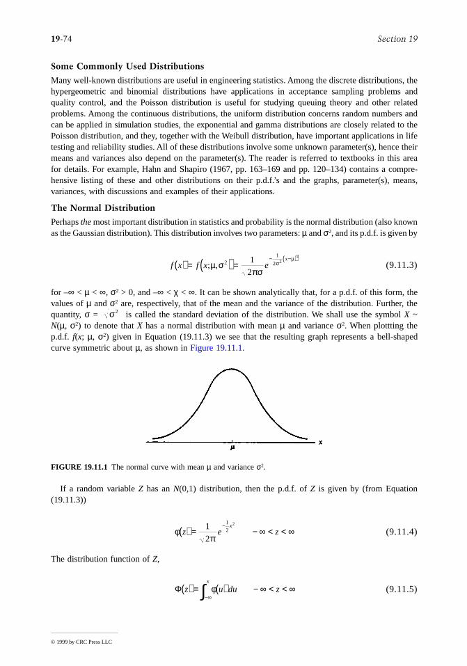
for –∞ < µ < ∞, σ2 > 0, and –∞ < χ < ∞. It can be shown analytically that, for a p.d.f. of this form, thevalues of µ and σ2 are, respectively, that of the mean and the variance of the distribution. Further, thequantity, σ = is called the standard deviation of the distribution. We shall use the symbol X ~N(µ, σ2) to denote that X has a normal distribution with mean µ and variance σ2. When plottting thep.d.f. f(x; µ, σ2) given in Equation (19.11.3) we see that the resulting graph represents a bell-shapedcurve symmetric about µ, as shown in Figure 19.11.1.
If a random variable Z has an N(0,1) distribution, then the p.d.f. of Z is given by (from Equation(19.11.3))
(9.11.4)
The distribution function of Z,
(9.11.5)
FIGURE 19.11.1 The normal curve with mean µ and variance σ2.
f x f x ex
( ) = ( ) =− −( )
; ,µ σπσ
σµ
21
21
22
2
σ2
φπ
z e zx
( ) = − ∞ < < ∞−1
2
1
22
Φ z u du zx
( ) = ( ) − ∞ < < ∞−∞∫ φ
Mathematics 19-75
© 1999 by CRC Press LLC
cannot be given in a closed form, hence it has been tabulated. The table of Φ(z) can be found in mosttextbooks in statistics and probability, including those listed in the references at the end of this section.(We note in passing that, by the symmetry property, Φ(z) + Φ(–z) = 1 holds for all z.)
Random Sample and Sampling Distributions
Random Sample and Related Statistics
As noted in Box et al., (1978), the design and analysis of engineering experiments usually involves thefollowing steps:
1. The choice of a suitable stochastic model by assuming that the observations follow a certaindistribution. The functional form of the distribution (or the p.d.f.) is assumed to be known, exceptthe value(s) of the parameters(s).
2. Design of experiments and collection of data.3. Summarization of data and computation of certain statistics.4. Statistical inference (including the estimation of the parameters of the underlying distribution and
the hypothesis-testing problems).
In order to make statistical inference concerning the parameter(s) of a distribution, it is essential tofirst study the sampling distributions. We say that X1, X2, …, Xn represent a random sample of size n ifthey are independent random variables and each of them has the same p.d.f., f(x). (Due to spacelimitations, the notion of independence will not be carefully discussed here. Nevertheless, we say thatX1, X2, …, Xn are independent if
(19.11.6)
holds for all sets A1, A2, …, An.) Since the parameter(s) of the population is (are) unknown, the populationmean µ and the population variance σ2 are unknown. In most commonly used distributions µ and σ2
can be estimated by the sample mean and the sample variance S2, respectively, which are given by
(19.11.7)
(The second equality in the formula for S2 can be verified algebraically.) Now, since X1, X2, …, Xn arerandom variables and S2 are also random variables. Each of them is called a statistic and has aprobability distribution which also involves the unknown parameter(s). In probability theory there aretwo fundamental results concerning their distributional properties.
Theorem 1. (Weak Law of Large Numbers). As the sample size n becomes large, converges to µin probability and S2 converges to σ2 in probability. More precisely, for every fixed positive number ε> 0 we have
(19.11.8)
as n → ∞.
Theorem 2. (Central Limit Theorem). As n becomes large, the distribution of the random variable
P X A X A X A P X An n i i
i
n
1 1 2 2
1
∈ ∈ ∈[ ] = ∈[ ]=
∏, , ,K
X
Xn
X Sn
X Xn
X nXi
i
n
i
i
n
i
i
n
= =−
−( ) =−
−
= = =
∑ ∑ ∑1 11
11
1
2 2
1
2 2
1
,
X
X
P X P S− ≤[ ] → − ≤[ ] →µ ε σ ε1 12 2,
19-76 Section 19
© 1999 by CRC Press LLC
(19.11.9)
has approximately an N(0,1) distribution. More precisely,
(19.11.10)
Normal Distribution-Related Sampling Distributions
One-Sample Case
Additional results exist when the observations come from a normal population. If X1, X2, …, Xn representa random sample of size n from an N(µ,σ2) population, then the following sample distributions are useful:
Fact 3. For every fixed n the distribution of Z given in Equation (19.11.9) has exactly an N(0,1)distribution.
Fact 4. The distribution of the statistic where is the sample standarddeviation, is called a Student’s t distribution with ν = n – 1 degrees of freedom, in symbols, t(n – 1).
This distribution is useful for making inference on µ when σ2 is unknown; a table of the percentilescan be found in most statistics textbooks.
Fact 5. The distribution of the statistic W = (n – 1)S2/σ2 is called a chi-squared distribution with ν =n – 1 degrees of freedom, in symbols χ2(ν). Such a distribution is useful in making inference on σ2; a table of the percentiles can also be found inmost statistics books.
Two-Sample Case
In certain applications we may be interested in the comparisons of two different treatments. Supposethat independent samples from treatments T1 and T2 are to be observed as shown in Table 19.11.1. .
The difference of the population means (µ1 – µ2) and the ratio of the population variances can beestimated, respectively, by and The following facts summarize the distributions ofthese statistics:
Fact 6. Under the assumption of normality, has an N(µ1 – µ2, distribu-tion; or equivalently, for all n1, n2 the statistic.
(19.11.11)
has an N(0,1) distribution.
Fact 7. When the common population variance is estimated by
(19.11.12)
TABLE 19.11.1 Summarization of Data for a Two-Sample Problem
Treatment Observations Distri bution Sample Size Sample Mean Sample Variance
T1 n1
T2 n2
ZX
n
n X= − =
−( )µσ
µσ
P Z z z z n≤[ ] → ( ) → ∞Φ for every fixed as
T n X S= −( )/ ,µ S S= 2
X X X n11 12 1 1
, , ,K N ( , )µ σ1 1
2X1
S12
X X X n21 22 2 2
, , ,K N ( , )µ σ2 2
2X2
S22
( )X X1 2− S S12
22/ .
( )X X1 2− ( / ) ( / ))σ σ12
1 22
2n n+
Z X X n n= −( ) − −( )[ ] +( )1 2 1 2 12
1 22
2
1 2µ µ σ σ
σ σ σ12
22 2= ≡ ,
S n n n S n Sp2
1 2
1
1 12
2 222 1 1= + −( ) −( ) + −( )[ ]−

Mathematics 19-77
© 1999 by CRC Press LLC
and has a χ2(n1 + n2 – 2) distribution.
Fact 8. When the statistic
(19.11.13)
has a t(n1 + n2 – 2) distribution, where
Fact 9. The distribution of is called an F distribution with degrees of freedom(n1 – 1, n2 – 1), in symbols, F(n1 – 1, n2 – 1),
The percentiles of this distribution have also been tabulated and can be found in statistics books.In the following two examples we illustrate numerically how to find probabilities and percentiles
using the existing tables for the normal, Student’s t, chi-squared, and F distributions.
Example 10. Suppose that in an experiment four observations are taken, and that the population isassumed to have a normal distribution with mean µ and variance σ2. Let and S2 be the sample meanand sample variance as given in Equation (19.11.7).
(a) If, based on certain similar experiments conducted in the past, we know that σ2 = 1.82 × 10⁻⁶ (σ= 1.8 × 10⁻³), then from Φ(–1.645) = 0.05 and Φ(1.96) = 0.975 we have
or equivalently,
(b) The statistic has a Student’s t distribution with 3 degrees of freedom (in symbols,t(3)). From the t table we have
which yields
or equivalently,
This is, in fact, the basis for obtaining the confidence interval for µ given in Equation (19.11.17) whenσ2 is unknown.
(c) The statistic 3S2/σ2 has a chi-squared distribution with 3 degrees of freedom (in symbols, χ2(3)).Thus from the chi-squared table we have P[0.216 ≤ 3S2/σ2 ≤ 9.348] = 0.95, which yields
( ) /n n Sp1 22 22+ − σ
σ σ12
22= ,
T X X S n np= −( ) − −( )[ ] +( )1 2 1 2 1 2
1 21 1µ µ
S Sp p= 2 .
F S S= ( / )/( / )12
12
22
22σ σ
X
PX− ≤ −
×≤
= − =−1 645
1 8 10 41 96 0 975 0 05 0 925
3.
.. . . .
µ
P X− × × ≤ − ≤ × ×[ ] =− −1 645 0 9 10 1 96 0 9 10 0 9253 3. . . . .µ
T X S= −2( )/µ
P X S− ≤ −( ) ≤[ ] =3 182 2 3 182 0 95. . .µ
PS
XS− × ≤ − ≤ ×
=3 1822
3 1822
0 95. . .µ
P XS
XS− × ≤ ≤ + ×
=3 1822
3 1822
0 95. . .µ
PS S3
9 3483
0 2160 95
22
2
. ..≤ ≤
=σ
19-78 Section 19
© 1999 by CRC Press LLC
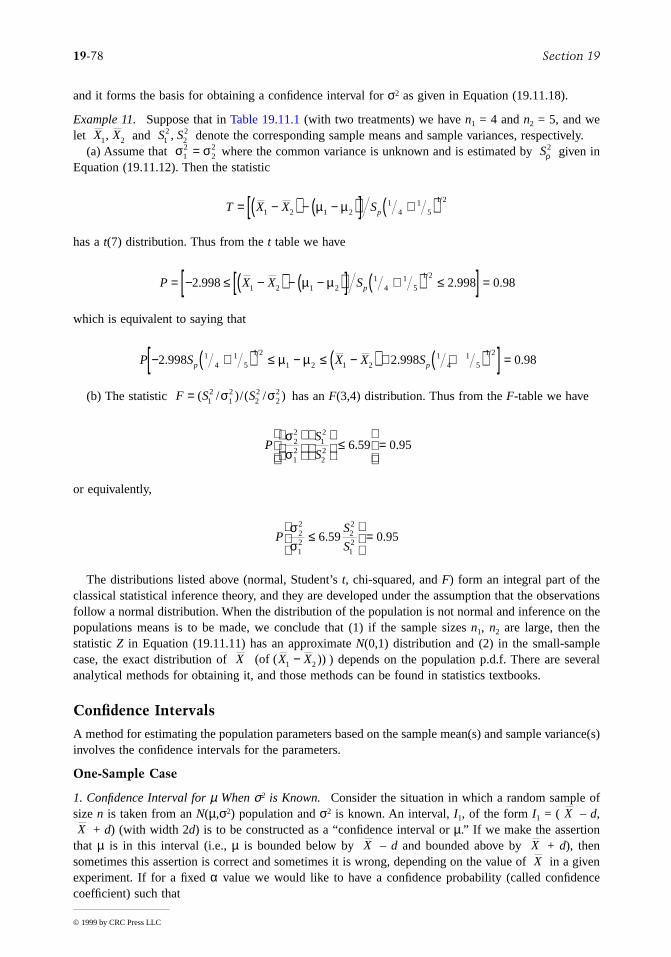
and it forms the basis for obtaining a confidence interval for σ2 as given in Equation (19.11.18).
Example 11. Suppose that in Table 19.11.1 (with two treatments) we have n1 = 4 and n2 = 5, and welet and denote the corresponding sample means and sample variances, respectively.
(a) Assume that where the common variance is unknown and is estimated by given inEquation (19.11.12). Then the statistic
has a t(7) distribution. Thus from the t table we have
which is equivalent to saying that
(b) The statistic has an F(3,4) distribution. Thus from the F-table we have
or equivalently,
The distributions listed above (normal, Student’s t, chi-squared, and F) form an integral part of theclassical statistical inference theory, and they are developed under the assumption that the observationsfollow a normal distribution. When the distribution of the population is not normal and inference on thepopulations means is to be made, we conclude that (1) if the sample sizes n1, n2 are large, then thestatistic Z in Equation (19.11.11) has an approximate N(0,1) distribution and (2) in the small-samplecase, the exact distribution of ) depends on the population p.d.f. There are severalanalytical methods for obtaining it, and those methods can be found in statistics textbooks.
Confidence Intervals
A method for estimating the population parameters based on the sample mean(s) and sample variance(s)involves the confidence intervals for the parameters.
One-Sample Case
1. Confidence Interval for µ When σ2 is Known. Consider the situation in which a random sample ofsize n is taken from an N(µ,σ2) population and σ2 is known. An interval, I1, of the form I1 = ( – d,
+ d) (with width 2d) is to be constructed as a “confidence interval or µ.” If we make the assertionthat µ is in this interval (i.e., µ is bounded below by – d and bounded above by + d), thensometimes this assertion is correct and sometimes it is wrong, depending on the value of in a givenexperiment. If for a fixed α value we would like to have a confidence probability (called confidencecoefficient) such that
X X1 2, S S12
22,
σ σ12
22= Sρ
2
T X X Sp= −( ) − −( )[ ] +( )1 2 1 21
41
5
1 2µ µ
P X X Sp= − ≤ −( ) − −( )[ ] +( ) ≤[ ] =2 998 2 998 0 981 2 1 21
41
5
1 2. . .µ µ
P S X X Sp p− +( ) ≤ − ≤ −( ) + +( )[ ] =2 998 2 998 0 9814
15
1 2
1 2 1 21
41
5
1 2. . .µ µ
F S S= ( / )/( / )12
12
22
22σ σ
PS
S
σσ
22
12
12
22 6 59 0 95
≤
=. .
PS
S
σσ
22
12
22
126 59 0 95≤
=. .
X (of ( ))X X1 2−
XX
X XX

Mathematics 19-79
© 1999 by CRC Press LLC
(19.11.14)
then we need to choose the value of d to satisfy i.e.,
(19.11.15)
where zα/2 is the (1 – α/2)th percentile of the N(0,1) distribution such that Φ(zα/2) = 1 – α/2. To see this,we note that from the sampling distribution of (Fact 3) we have
(19.11.16)
We further note that, even when the original population is not normal, by Theorem 2 the confidenceprobability is approximately (1 – α) when the sample size is reasonably large.
2. Confidence Interval for µ When σ 2 is Unknown. Assume that the observations are from an N(µ,σ2)population. When σ2 is unknown, by Fact 4 and a similar argument we see that
(19.11.17)
is a confidence interval for µ with confidence probability 1 – α, where tα/2(n – 1) is the (1 – α/2)thpercentile of the t(n – 1) distribution.
3. Confidence Interval for σ 2. If, under the same assumption of normality, a confidence interval for σ2
is needed when µ is unknown, then
(19.11.18)
has a confidence probability 1 – α, when (n – 1) and (n – 1) are the (α/2)th and (1 – α/2)thpercentiles, respectively, of the χ2(n – 1) distribution.
Two-Sample Case
1. Confidence Intervals for µ1 – µ2 When are Known. Consider an experiment that involvesthe comparison of two treatments, T1 and T2, as indicated in Table 19.11.1. If a confidence interval forδ = µ1 – µ2 is needed when and are unknown, then by Fact 6 and a similar argument, theconfidence interval
(19.11.19)
has a confidence probability 1 – α.
2. Confidence Interval for µ1 – µ2 when are Unknown but Equal. Under the add i t i ona lassumption that but the common variance is unknown, then by Fact 8 the confidence interval
P I P X d X dµ µ α∈[ ] = − < < +[ ] = −1 1
d zn
= ασ
2 ,
I X zn
X zn1 2 2= − +
α α
σ σ,
X
P X zn
X zn
PX
nz
z z
− < < +
=−
≤
= ( ) − −( ) = −
α α α
α α
σ µ σ µ
σ
α
2 2 2
2 2 1Φ Φ
I X t nS
nX t n
S
n2 2 21 1= − −( ) + −( )
α α,
I n S n n S n32
1 22 2
221 1 1 1= −( ) −( ) −( ) −( )( )−χ χα α,
χ α1 22− χα 2
2
σ σ12
22=
σ12 σ2
2
I X X z n n X X z n n4 1 2 2 12
1 22
2 1 2 2 12
1 22
2= −( ) − + −( ) + +( )α ασ σ σ σ,
σ σ12
22,
σ σ12
22= ,
19-80 Section 19
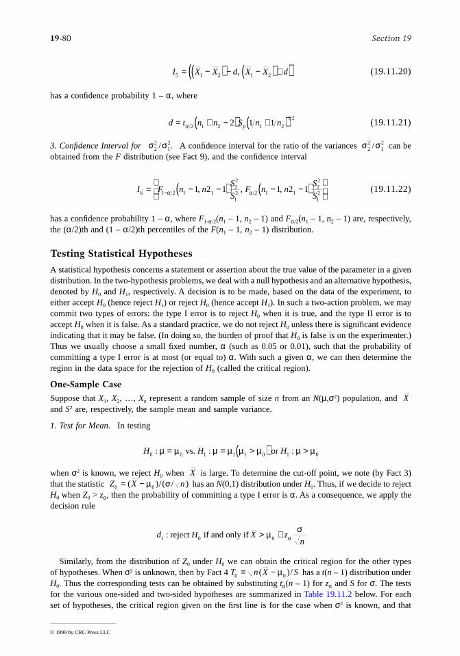
© 1999 by CRC Press LLC
(19.11.20)
has a confidence probability 1 – α, where
(19.11.21)
3. Confidence Interval for . A confidence interval for the ratio of the variances can beobtained from the F distribution (see Fact 9), and the confidence interval
(19.11.22)
has a confidence probability 1 – α, where F1-α/2(n1 – 1, n2 – 1) and Fα/2(n1 – 1, n2 – 1) are, respectively,the (α/2)th and (1 – α/2)th percentiles of the F(n1 – 1, n2 – 1) distribution.
Testing Statistical Hypotheses
A statistical hypothesis concerns a statement or assertion about the true value of the parameter in a givendistribution. In the two-hypothesis problems, we deal with a null hypothesis and an alternative hypothesis,denoted by H0 and H1, respectively. A decision is to be made, based on the data of the experiment, toeither accept H0 (hence reject H1) or reject H0 (hence accept H1). In such a two-action problem, we maycommit two types of errors: the type I error is to reject H0 when it is true, and the type II error is toaccept H0 when it is false. As a standard practice, we do not reject H0 unless there is significant evidenceindicating that it may be false. (In doing so, the burden of proof that H0 is false is on the experimenter.)Thus we usually choose a small fixed number, α (such as 0.05 or 0.01), such that the probability ofcommitting a type I error is at most (or equal to) α. With such a given α, we can then determine theregion in the data space for the rejection of H0 (called the critical region).
One-Sample Case
Suppose that X1, X2, …, Xn represent a random sample of size n from an N(µ,σ2) population, and and S2 are, respectively, the sample mean and sample variance.
1. Test for Mean. In testing
when σ2 is known, we reject H0 when is large. To determine the cut-off point, we note (by Fact 3)that the statistic has an N(0,1) distribution under H0. Thus, if we decide to rejectH0 when Z0 > zα, then the probability of committing a type I error is α. As a consequence, we apply thedecision rule
Similarly, from the distribution of Z0 under H0 we can obtain the critical region for the other typesof hypotheses. When σ2 is unknown, then by Fact 4 has a t(n – 1) distribution underH0. Thus the corresponding tests can be obtained by substituting tα(n – 1) for zα and S for σ. The testsfor the various one-sided and two-sided hypotheses are summarized in Table 19.11.2 below. For eachset of hypotheses, the critical region given on the first line is for the case when σ2 is known, and that
I X X d X X d5 1 2 1 2= −( ) − −( ) +( ),
d t n n S n np= + −( ) +( )α 2 1 2 1 2
1 22 1 1
σ σ22
12/ σ σ2
212/
I F n nS
SF n n
S
S6 1 2 1 122
12 2 1 1
22
121 2 1 1 2 1= − −( ) − −( )
−α α, , ,
X
H H H0 0 1 1 1 0 1 0: : :µ µ µ µ µ µ µ µ= = >( ) > vs. or
XZ X n0 0= −( )/( / )µ σ
d H X zn1 0 0: reject if and only if > +µ σ
α
T n X S0 0= −( )/µ

Mathematics 19-81
© 1999 by CRC Press LLC
given on the second line is for the case when σ2 is unknown. Furthermore, tα and tα/2 stand for tα(n –1) and tα/2(n – 1), respectively.
2. Test for Variance. In testing hypotheses concerning the variance σ2 of a normal distribution, use Fact5 to assert that, under H0: σ2 = the distribution of w0 = (n – 1) is χ2(n – 1). The correspondingtests and critical regions are summarized in the following table and stand for (n – 1) and
(n – 1), respectively):
Two-Sample Case
In comparing the means and variances of two normal populations, we once again refer to Table 19.11.1for notation and assumptions.
1. Test for Difference of Two Means. Let δ = µ1 – µ2 be the difference of the two population means.In testing H0: δ = δ0 vs. a one-sided or two-sided alternative hypothesis, we note that, for
(19.11.23)
and
(19.11.24)
TABLE 19.11.2 One-Sample Tests for Mean
Null Hypothesis H0 Alternative Hypothesis H1 Critical Region
µ = µ0 or µ ≤ µ0 µ = µ1 > µ0 or µ > µ0
µ = µ0 or µ ≥ µ0 µ = µ1 < µ0 or µ < µ0
µ = µ0 µ ≠ µ0
TABLE 19.11.3 One-Sample Tests for Variance
Null Hypothesis H0 Alternative Hypothesis H1 Critical Region
X zn
> +µ σα0
X tS
n> +µ α0
X zn
< −µ σα0
X tS
n< −µ α0
X zn
− >µ σα0 2/
X tS
n− >µ α0 2/
σ02 , S2
02/σ
(χα2 χα / 2
2 χα2
χα / 22
σ σ σ σ202 2
02= ≤ or σ σ σ σ σ2
12
02 2
02= >> or S
n2
02 21
1σ χα( ) >
−
σ σ σ σ202 2
02= ≥ or σ σ σ σ σ2
12
02 2
02= << or S
n2
02
121
1σ χ α( ) <
− −
σ σ202= σ σ2
02≠ S
n2
02
221
1σ χα( ) >
− /
or Sn
202
1 221
1σ χ α( ) <
− − /
τ σ σ= +( )12
1 22
2
1 2n n
ν = +( )S n np 1 11 2
1 2

19-82 Section 19
© 1999 by CRC Press LLC
Z0 = [ – δ0]/τ has an N(0,1) distribution under H0 and T0 = [ – δ0]/ν has a t(n1 +n2 – 2) distribution under H0 when Using these results, the corresponding critical regions forone-sided and two-sided tests can be obtained, and they are listed below. Note that, as in the one-samplecase, the critical region given on the first line for each set of hypotheses is for the case of knownvariances, and that given on the second line is for the case in which the variances are equal but unknown.Further, tα and tα/2 stand for tα(n1 + n2 – 2) and tα/2(n1 + n2 – 2), respectively.
A Numerical Example
In the following we provide a numerical example for illustrating the construction of confidence intervalsand hypothesis-testing procedures. The example is given along the line of applications in Wadsworth(1990, p. 4.21) with artificial data.
Suppose that two processes (T1 and T2) manufacturing steel pins are in operation, and that a randomsample of 4 pins (or 5 pins) was taken from the process T1 (the process T2) with the following results(in units of inches):
Simple calculation shows that the observed values of sample means sample variances, and samplestandard deviations are:
One-Sample Case
Let us first consider confidence intervals for the parameters of the first process, T1, only.
1. Assume that, based on previous knowledge of processes of this type, the variance is known tobe = 1.802 × 10⁻⁶ (σ1 = 0.0018). Then from the normal table (see, e.g., Ross (1987, p. 482)we have z0.025 = 1.96. Thus a 95% confidence interval for µ1 is
TABLE 19.11.4 Two-Sample Tests for Difference of Two Means
Null Hypothesis H0 Alternative Hypothesis H1 Critical Region
δ = δ or δ ≤ δ0 δ = δ1 > δ0 or δ > δ0
δ = δ0 or δ ≥ δ0 δ = δ1 < δ0 or δ < δ0
δ = δ0 δ ≠ δ0
( )X X1 2− ( )X X1 2−σ σ1
222= .
X X z1 2 0−( ) > +δ τα
X X t1 2 0−( ) > +δ να
X X z1 2 0−( ) < −δ τα
X X t1 2 0−( ) < −δ να
X X z1 2 0 2−( ) − >δ τα /
X X t1 2 0 2−( ) − >δ να /
T
T
1
2
0 7608 0 7596 0 7622 0 7638
0 7546 0 7561 0 7526 0 7572 0 7565
: . , . , . , .
: . , . , . , . , .
X S S
X S S
1 12 6
13
2 22 6
23
0 7616 3 280 10 1 811 10
0 7554 3 355 10 1 832 10
= = × = ×
= = × = ×
− −
− −
. , . , .
. , . , .
σ12
0 7616 1 96 0 0018 4 0 7616 1 96 0 0018 4. . . , . . .− × + ×( )

Mathematics 19-83
© 1999 by CRC Press LLC
or (0.7598, 0.7634) (after rounding off to the 4th decimal place).2. If is unknown and a 95% confidence interval for µ1 is needed then, for t0.023 (3) = 3.182 (see,
e.g., Ross, 1987, p. 484) the confidence interval is
or (0.7587, 0.7645)3. From the chi-squared table with 4 – 1 = 3 degrees of freedom, we have (see, e.g., Ross, 1987, p.
483) = 0.216, = 9.348. Thus a 95% confidence interval for is (3 × 3.280 ×10–6/9.348, 3 × 3.280 × 10–6/0.216), or (1.0526 × 10⁻⁶, 45,5556 × 10⁻⁶).
4. In testing the hypotheses
with a = 0.01 when is unknown, the critical region is > 0.76 + 4.541 × 0.001811/ =0.7641. Since the observed value is 0.7616, H0 is accepted. That is, we assert that there is nosignificant evidence to call for the rejection of H0.
Two-Sample Case
If we assume that the two populations have a common unknown variance, we can use the Student’s tdistribution (with degree of freedom ν = 4 + 5 – 2 = 7) to obtain confidence intervals and to testhypotheses for µ1 – µ2. We first note that the data given above yield
and = 0.0062.
1. A 98% confidence interval for µ1 – µ2 is (0.0062 – 2.998ν, 0.0062 + 2.998ν) or (0.0025, 0.0099).2. In testing the hypotheses H0: µ1 = µ2 (i.e., µ1 – µ2 = 0) vs. H1: µ1 > µ2 with α = 0.05, the critical
region is > 1.895ν = 2.3172 × 10⁻³. Thus H0 is rejected; i.e., we conclude that thereis significant evidence to indicate that µ1 > µ2 may be true.
3. In testing the hypotheses H0: µ1 = µ2 vs. µ1 ≠ µ2 with α = 0.02, the critical region is > 2.998ν = 3.6660 × 10⁻³. Thus H0 is rejected. We note that the conclusion here is consistentwith the result that, with confidence probability 1 – α = 0.98, the confidence interval for (µ1 –µ2) does not contain the origin.
Concluding Remarks
The history of probability and statistics goes back to the days of the celebrated mathematicians K. F.Gauss and P. S. Laplace. (The normal distribution, in fact, is also called the Gaussian distribution.) Thetheory and methods of classical statistical analysis began its developments in the late 1800s and early1900s when F. Galton and R.A. Fisher applied statistics to their research in genetics, when Karl Pearsondeveloped the chi-square goodness-of-fit method for stochastic modeling, and when E.S. Pearson andJ. Neyman developed the theory of hypotheses testing. Today statistical methods have been found usefulin analyzing experimental data in biological science and medicine, engineering, social sciences, andmany other fields. A non-technical review on some of the applications is Hacking (1984).
σ12
0 7616 3 182 0 001811 4 0 7616 3 182 0 001811 4. . . , . . .− × + ×( )
χ0 9752
. χ0 0252
. σ12
H H0 1 1 10 76 0 76: . : .µ µ= > vs.
σ12 x1 4
x1
S
S S
p
p p
2 6
6
3 3
17
3 3 280 4 3 355 10
3 3229 10
1 8229 10 1 4 1 5 1 2228 10
= × + ×( ) ×
= ×
= × = + = ×
−
−
− −
. .
.
. .ν
X X1 2−
( )X X1 2−
| |X X1 2−

19-84 Section 19
© 1999 by CRC Press LLC
Applications of statistics in engineering include many topics. In addition to those treated in thissection, other important ones include sampling inspection and quality (process) control, reliability,regression analysis and prediction, design of engineering experiments, and analysis of variance. Due tospace limitations, these topics are not treated here. The reader is referred to textbooks in this area forfurther information. There are many well-written books that cover most of these topics, the followingshort list consists of a small sample of them.
References
Box, G.E.P., Hunter, W.G., and Hunter, J.S. 1978. Statistics for Experimenters. John Wiley & Sons, NewYork.
Bowker, A.H. and Lieberman, G.J. 1972. Engineering Statistics, 2nd ed. Prentice-Hall, Englewood Cliffs,NJ.
Hacking, I. 1984. Trial by number, Science, 84(5), 69–70.Hahn, G.J. and Shapiro, S.S. 1967. Statistical Models in Engineering. John Wiley & Sons, New York.Hines, W.W. and Montgomery, D.G. 1980. Probability and Statistics in Engineering and Management
Science. John Wiley & Sons, New York.Hogg, R.V. and Ledolter, J. 1992. Engineering Statistics. Macmillan, New York.Ross, S.M. 1987. Introduction to Probability and Statistics for Engineers and Scientists. John Wiley &
Sons, New York.Wadsworth, H.M., Ed. 1990. Handbook of Statistical Methods for Engineers and Scientists. John Wiley
& Sons, New York.

Mathematics 19-85
© 1999 by CRC Press LLC
19.12 Numerical Methods
William F. Ames
Introduction
Since many mathematical models of physical phenomena are not solvable by available mathematicalmethods one must often resort to approximate or numerical methods. These procedures do not yieldexact results in the mathematical sense. This inexact nature of numerical results means we must payattention to the errors. The two errors that concern us here are round-off errors and truncation errors.
Round-off errors arise as a consequence of using a number specified by m correct digits to approximatea number which requires more than m digits for its exact specification. For example, using 3.14159 toapproximate the irrational number π. Such errors may be especially serious in matrix inversion or inany area where a very large number of numerical operations are required. Some attempts at handlingthese errors are called enclosure methods. (Adams and Kulisch, 1993).
Truncation errors arise from the substitution of a finite number of steps for an infinite sequence ofsteps (usually an iteration) which would yield the exact result. For example, the iteration yn(x) = 1+ xtyn–1(t)dt, y(0) = 1 is only carried out for a few steps, but it converges in infinitely many steps.
The study of some errors in a computation is related to the theory of probability. In what follows, arelation for the error will be given in certain instances.
Linear Algebra Equations
A problem often met is the determination of the solution vector u = (u1, u2, …, un)T for the set of linearequations Au = v where A is the n × n square matrix with coefficients, aij (i, j = 1, …, n), v = (v1, …,vn)T and i denotes the row index and j the column index.
There are many numerical methods for finding the solution, u, of Au = v. The direct inversion of Ais usually too expensive and is not often carried out unless it is needed elsewhere. We shall only list afew methods. One can check the literature for the many methods and computer software available. Someof the software is listed in the References section at the end of this chapter. The methods are usuallysubdivided into direct (once through) or iterative (repeated) procedures.
In what follows, it will often be convenient to partition the matrix A into the form A = U + D + L,where U, D, and L are matrices having the same elements as A, respectively, above the main diagonal,on the main diagonal, and below the main diagonal, and zeros elsewhere. Thus,
We also assume the ujs are not all zero and det A ≠ 0 so the solution is unique.
Direct Methods
Gauss Reduction.This classical method has spawned many variations. It consists of dividing the firstequation by a11 (if a11 = 0, reorder the equations to find an a11 ≠ 0) and using the result to eliminate theterms in u1 from each of the succeeding equations. Next, the modified second equation is divided by
(if = 0, a reordering of the modified equations may be necessary) and the resulting equation isused to eliminate all terms in u2 in the succeeding modified equations. This elimination is done n timesresulting in a triangular system:
∫ 0x
U
a a
a an
n=
0
0 0
0 0 0
12 1
23 2
L
L
M L L
L L
′a22 ′a22
19-86 Section 19
© 1999 by CRC Press LLC
where and represent the specific numerical values obtained by this process. The solution is obtainedby working backward from the last equation. Various modifications, such as the Gauss-Jordan reduction,the Gauss-Doolittle reduction, and the Crout reduction, are described in the classical reference authoredby Bodewig (1956). Direct methods prove very useful for sparse matrices and banded matrices that oftenarise in numerical calculation for differential equations. Many of these are available in computer packagessuch as IMSL, Maple, Matlab, and Mathematica.
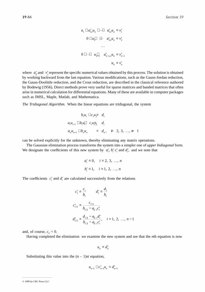
The Tridiagonal Algorithm.When the linear equations are tridiagonal, the system
can be solved explicitly for the unknown, thereby eliminating any matrix operations.The Gaussian elimination process transforms the system into a simpler one of upper bidiagonal form.
We designate the coefficients of this new system by and we note that
The coefficients are calculated successively from the relations
and, of course, cn = 0.Having completed the elimination we examine the new system and see that the nth equation is now
Substituting this value into the (n – 1)st equation,
u a u a u v
u a u v
u a u v
u v
n n
n n
n n n n n
n n
1 12 2 1 1
2 2 2
1 1 1
0
0
+ ′ + + ′ = ′
+ + + ′ = ′
+ + + ′ = ′
= ′
− − −
L
L
L
L ,
′aij ′vj
b u c u d
a u b u c u d
a u b u d i n
i i i i i i i
n n n n n
1 1 1 2 1
1 1
1
+ =
+ + =
+ = = −
− +
− , 2, 3, , 1K
′ ′ ′ ′a b c di i i i, ,and
′ = =
′ = =
a i n
b i n
i
i
0
1
,
,
2, 3, ,
1, 2, ,
K
K
′ ′c di iand
′ = ′ =
′ =− ′
′ =− ′− ′
= −
++
+ +
++ +
+ +
cc
bd
d
b
cc
b a c
dd a d
b a ci n
ii
i i i
ii i i
i i i
11
11
1
1
11
1 1
11 1
1 1
, 1, 2, , 1K
u dn n= ′
u c u dn n n n− − −+ ′ = ′1 1 1

Mathematics 19-87
© 1999 by CRC Press LLC
we have
Thus, starting with un, we have successively the solution for ui as
Algorithm for Pentadiagonal Matrix.The equations to be solved are
for 1 ≤ i ≤ R with a1 = b1 = a2 = eR–1 = dR = eR = 0.The algorithm is as follows. First, compute
and
Then, for 3 ≤ i ≤ R – 2, compute
Next, compute
u d c un n n n− − −= ′ − ′1 1 1
u d c u i n ni i i i= ′ − ′ = − −+1 1, , 2, , 1K
a u b u c u d u e u fi i i i i i i i i i i− − + ++ + + + =2 1 1 2
δ
λ
γ
1 1 1
1 1 1
1 1 1
=
=
=
d c
e c
f c
µ δ
δ λ µ
λ µ
γ γ µ
2 2 2 1
2 2 2 1 2
2 2 2
2 2 1 2
= −
= −( )=
= −( )
c b
d b
e
f b
β δ
µ β δ λ
δ β λ µ
λ µ
γ β γ γ µ
i i i i
i i i i i i
i i i i i
i i i
i i i i i i i
b a
c a
d
e
f a
= −
= − −
= −( )=
= − −( )
−
− −
−
− −
2
1 2
1
1 2
β δ
µ β δ λ
δ β λ µ
γ β γ γ µ
R R R R
R R R R R R
R R R R R
R R R R R R R
b a
c a
d
f a
− − − −
− − − − − −
− − − − −
− − − − − − −
= −
= − −
= −( )= − −( )
1 1 1 3
1 1 1 2 1 3
1 1 1 2 1
1 1 1 2 1 3 1

19-88 Section 19
© 1999 by CRC Press LLC
and
The βi and µi are used only to compute δi, λ i, and γi, and need not be stored after they are computed.The δi, λ i, and γi, must be stored, as they are used in the back solution. This is
and
for R – 2 ≥ i ≥ 1.
General Band Algorithm.The equations are of the form
for 1 ≤ j ≤ N, N ≥ M. The algorithm used is as follows:
The forward solution (j = 1, …, N) is
The back solution (j = N, …, 1) is
β δ
µ β δ λ
γ β γ γ µ
R R R R
R R R R R R
R R R R R R R
b a
c a
f a
= −
= − −
= − −( )
−
− −
− −
2
1 2
1 2
u
u u
R R
R R R R
=
= −− − −
γ
γ δ1 1 1
u u ui i i i i i= − −+ +γ δ λ1 2
A X A X A X A X B X
C X C X C X C X D
jM
j M jM
j M j j j j j j
j j j j jM
j M jM
j M j
( )−
−( )− +
( )−
( )−
( )+
( )+
−( )+ −
( )+
+ + + + +
+ + + + + =
11
22
11
11
22
11
L
L
α jk
jk
jk
A k j
C k N j
( ) ( )
( )
= = ≥
= ≥ + −
0
0 1
,
,
for
for
α α
β α
α β
jk
jk
jp
p k
p M
j pp k
j j jp
p
M
j pp
jk
jk
jp k
p k
p M
j p k
pj
A W k M
B W
W C W k
( ) ( ) ( )
= +
=
−−( )
( )
=−( )
( ) ( ) −( )
= +
=
− −( )( )
= − =
= −
= −
∑
∑
∑
1
1
1
1, , ,
,
K
==
= −
( )
=−∑
1
1
, ,K M
Dj j jp
p
M
j p jγ α γ β

Mathematics 19-89
© 1999 by CRC Press LLC
Cholesky Decomposition.When the matrix A is a symmetric and positive definite, as it is for manydiscretizations of self-adjoint positive definite boundary value problems, one can improve considerablyon the band procedures by using the Cholesky decomposition. For the system Au = v, the Matrix A canbe written in the form
where L is lower triangular, U is upper triangular, and D is diagonal. If A = A′ (A′ represents the transposeof A), then
Hence, because of the uniqueness of the decomposition.
and therefore,
that is,
The system Au = v is then solved by solving the two triangular system
followed by
To carry out the decomposition A = B′B, all elements of the first row of A, and of the derived system,are divided by the square root of the (positive) leading coefficient. This yields smaller rounding errorsthan the banded methods because the relative error of is only half as large as that of a itself. Also,taking the square root brings numbers nearer to each other (i.e., the new coefficients do not differ aswidely as the original ones do). The actual computation of B = (bij), j > i, is given in the following:
X W Xj j jp
p
M
j p= − ( )
=+∑γ
1
A I L D I U= +( ) +( )
A A I U D I L= ′ = +( )′ +( )′
I L I U I U+ = +( )′ = + ′
A I U D I U= +( )′ +( )
A B B B D I U= ′ = +( ), where
′ =B w v
Bu w=
a
19-90 Section 19
© 1999 by CRC Press LLC
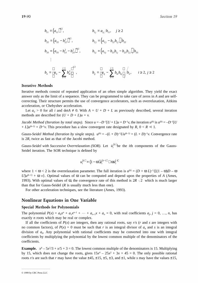
Iterative Methods
Iterative methods consist of repeated application of an often simple algorithm. They yield the exactanswer only as the limit of a sequence. They can be programmed to take care of zeros in A and are self-correcting. Their structure permits the use of convergence accelerators, such as overrelaxation, Aitkinsacceleration, or Chebyshev acceleration.
Let aii > 0 for all i and detA ≠ 0. With A = U + D + L as previously described, several iterationmethods are described for (U + D + L)u = v.
Jacobi Method (Iteration by total steps).Since u = –D–1[U + L]u + D–1v, the iteration u(k) is u(k) = –D–1[U+ L]u(k–1) + D–1v. This procedure has a slow convergent rate designated by R, 0 < R ! 1.
Gauss-Seidel Method (Iteration by single steps). u(k) = –(L + D)–1Uu(k–1) + (L + D)–1v. Convergence rateis 2R, twice as fast as that of the Jacobi method.
Gauss-Seidel with Successive Overrelaxation (SOR).Let be the ith components of the Gauss-Seidel iteration. The SOR technique is defined by
where 1 < ω < 2 is the overrelaxation parameter. The full iteration is u(k) = (D + ω L)–1{[(1 – ω)D – ωU]u(k–1) + ω v}. Optimal values of ω can be computed and depend upon the properties of A (Ames,1993). With optimal values of ω, the convergence rate of this method is 2R which is much largerthan that for Gauss-Seidel (R is usually much less than one).
For other acceleration techniques, see the literature (Ames, 1993).
Nonlinear Equations in One Variable
Special Methods for Polynomials
The polynomial P(x) = a0xn + a1xn–1 + L + an–1x + an = 0, with real coefficients aj, j = 0, …, n, hasexactly n roots which may be real or complex.
If all the coefficients of P(x) are integers, then any rational roots, say r/s (r and s are integers withno common factors), of P(x) = 0 must be such that r is an integral divisor of an and s is an integraldivision of a0. Any polynomial with rational coefficients may be converted into one with integralcoefficients by multiplying the polynomial by the lowest common multiple of the denominators of thecoefficients.
Example. x4 – 5x2/3 + x/5 + 3 = 0. The lowest common multiple of the denominators is 15. Multiplyingby 15, which does not change the roots, gives 15x4 – 25x2 + 3x + 45 = 0. The only possible rationalroots r/s are such that r may have the value ±45, ±15, ±5, ±3, and ±1, while s may have the values ±15,
b a b a b j
b a b b a b b b
b a b b b a b b b b b
b a b
j ij
j j j
j j j j
ii ii ki
k
i
11 11
1 2
1 11
22 22 122 1 2
2 2 12 1 22
33 33 132
232 1 2
3 3 13 1 23 2 33
2
1
1
2= ( ) = ≥
= −( ) = −( )= − −( ) = − −( )
= −
=
−
∑
, ,
,
,
M
= −
≥ ≥
=
−
∑1 2
1
1
2 2, , ,b a b b b i jij ij ki kj
k
i
ii
uik( )
u u uik
ik
ik( ) −( ) ( )= −( ) +1 1ω ω
2

Mathematics 19-91
© 1999 by CRC Press LLC
±5, ±3, and ±1. All possible rational roots, with no common factors, are formed using all possiblequotients.
If a0 > 0, the first negative coefficient is preceded by k coefficients which are positive or zero, and Gis the largest of the absolute values of the negative coefficients, then each real root is less than 1 +
(upper bound on the real roots). For a lower bound to the real roots, apply the criterion toP(–x) = 0.
Example. P(x) = x5 + 3x4 – 2x3 – 12x + 2 = 0. Here a0 = 1, G = 12, and k = 2. Thus, the upper boundfor the real roots is 1 + ≈ 4.464. For the lower bound, P(–x) = –x5 + 3x4 + 2x3 + 12x + 2 = 0,which is equivalent to x5 – 3x4 – 2x3 – 12x – 2 = 0. Here k = 1, G = 12, and a0 = 1. A lower bound is–(1 + 12) = 13. Hence all real roots lie in –13 < x < 1 +
A useful Descartes rule of signs for the number of positive or negative real roots is available byobservation for polynomials with real coefficients. The number of positive real roots is either equal tothe number of sign changes, n, or is less than n by a positive even integer. The number of negative realroots is either equal to the number of sign changes, n, of P(–x), or is less than n by a positive even integer.
Example. P(x) = x5 – 3x3 – 2x2 + x – 1 = 0. There are three sign changes, so P(x) has either three orone positive roots. Since P(–x) = –x5 + 3x3 – 2x2 – 1 = 0, there are either two or zero negative roots.
The Graeffe Root-Squaring Technique
This is an iterative method for finding the roots of the algebraic equation
If the roots are r1, r2, r3, …, then one can write
and if one root is larger than all the others, say r1, then for large enough p all terms (other than 1) wouldbecome negligible. Thus,
or
The Graeffe procedure provides an efficient way for computing Sp via a sequence of equations such thatthe roots of each equation are the squares of the roots of the preceding equations in the sequence. Thisserves the purpose of ultimately obtaining an equation whose roots are so widely separated in magnitudethat they may be read approximately from the equation by inspection. The basic procedure is illustratedfor a polynomial of degree 4:
Rewrite this as
G ak / 0
122
122 .
f x a x a x a x ap p
p p( ) = + + + + =−−0 1
11 0L
S rr
r
r
rpp
p
p
p
p= + + +
12
1
3
1
1 L
S rpp≈ 1
limp p
pS r→∞
=11
f x a x a x a x a x a( ) = + + + + =04
13
22
3 4 0
a x a x a a x a x04
22
4 13
3+ + = − −
19-92 Section 19
© 1999 by CRC Press LLC
and square both sides so that upon grouping
Because this involves only even powers of x, we may set y = x2 and rewrite it as
whose roots are the squares of the original equation. If we repeat this process again, the new equationhas roots which are the fourth power, and so on. After p such operations, the roots are 2p (original roots).If at any stage we write the coefficients of the unknown in sequence
then, to get the new sequence write (times the symmetric coefficient) with respectto – (times the symmetric coefficient) – L (–1)i Now if the roots are r1, r2, r3, and r4,then a1/a0 = – If the roots are all distinct and r1 is thelargest in magnitude, then eventually
And if r2 is the next largest in magnitude, then
And, in general This procedure is easily generalized to polynomials of arbitrary degreeand specialized to the case of multiple and complex roots.
Other methods include Bernoulli iteration, Bairstow iteration, and Lin iteration. These may be foundin the cited literature. In addition, the methods given below may be used for the numerical solution ofpolynomials.
General Methods for Nonlinear Equations in One Variable
Successive Substitutions
Let f(x) = 0 be the nonlinear equation to be solved. If this is rewritten as x = F(x), then an iterativescheme can be set up in the form xk+1 = F(xk). To start the iteration, an initial guess must be obtainedgraphically or otherwise. The convergence or divergence of the procedure depends upon the method ofwriting x = F(x), of which there will usually be several forms. A general rule to ensure convergencecannot be given. However, if a is a root of f(x) = 0, a necessary condition for convergence is that |F′(x)|< 1 in that interval about a in which the iteration proceeds (this means the iteration cannot convergeunless |F′(x)| < 1, but it does not ensure convergence). This process is called first order because the errorin xk+1 is proportional to the first power of the error in xk.
Example. f(x) = x3 – x – 1 = 0. A rough plot shows a real root of approximately 1.3. The equationcan be written in the form x = F(x) in several ways, such as x = x3 – 1, x = 1/(x2 – 1), and x = (1 +x)1/3. In the first case, F′(x) = 3x2 = 5.07 at x = 1.3; in the second, F′(1.3) = 5.46; only in the third case
a x a a a x a a a a a x a a a x a02 8
0 2 12 6
0 4 1 3 22 4
2 4 32 2
422 2 2 2 0+ −( ) + − +( ) + −( ) + =
a y a a a y a a a a a y a a a y a02 4
0 2 12 3
0 4 1 3 22 2
2 4 32
422 2 2 2 0+ −( ) + − +( ) + −( ) + =
a a a a ap p p p p0 1 2 3 4( ) ( ) ( ) ( ) ( )
aip( ) ,+1 a ai
p p( ) ( )+ =102
aip( ) 2 1a p( ) ai
p( ) .2
Σ Σ Σi i i i ip p
ipr a a r a a r− = − = −1
4 101 2
02, / , , / .( ) ( ) ( ) ( )K
ra
ap
p
p12 1
0
≈ −( )
( )
ra
ap
p
p22 2
1
≈ −( )
( )
a a rnp
np
np( ) ( )/ .− ≈ −1
2
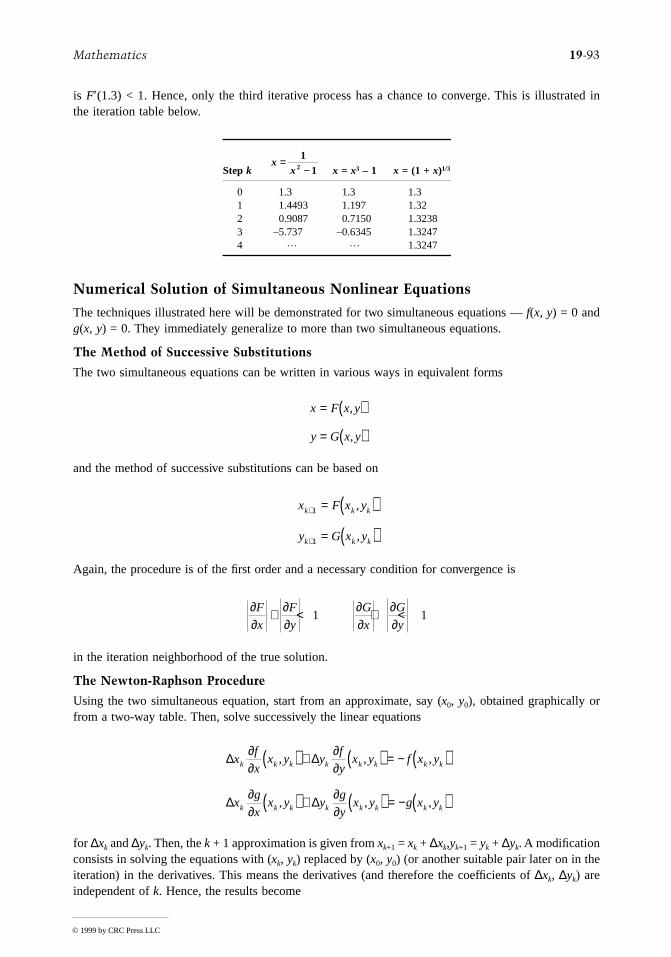
Mathematics 19-93
© 1999 by CRC Press LLC
is F′(1.3) < 1. Hence, only the third iterative process has a chance to converge. This is illustrated inthe iteration table below.
Numerical Solution of Simultaneous Nonlinear Equations
The techniques illustrated here will be demonstrated for two simultaneous equations — f(x, y) = 0 andg(x, y) = 0. They immediately generalize to more than two simultaneous equations.
The Method of Successive Substitutions
The two simultaneous equations can be written in various ways in equivalent forms
and the method of successive substitutions can be based on
Again, the procedure is of the first order and a necessary condition for convergence is
in the iteration neighborhood of the true solution.
The Newton-Raphson Procedure
Using the two simultaneous equation, start from an approximate, say (x0, y0), obtained graphically orfrom a two-way table. Then, solve successively the linear equations
for ∆xk and ∆yk. Then, the k + 1 approximation is given from xk+1 = xk + ∆xk,yk+1 = yk + ∆yk. A modificationconsists in solving the equations with (xk, yk) replaced by (x0, y0) (or another suitable pair later on in theiteration) in the derivatives. This means the derivatives (and therefore the coefficients of ∆xk, ∆yk) areindependent of k. Hence, the results become
Step k x = x3 – 1 x = (1 + x)1/3
0 1.3 1.3 1.31 1.4493 1.197 1.322 0.9087 0.7150 1.32383 –5.737 –0.6345 1.32474 L L 1.3247
xx
=−
112
x F x y
y G x y
= ( )
= ( )
,
,
x F x y
y G x y
k k k
k k k
+
+
= ( )= ( )
1
1
,
,
∂∂
∂∂
∂∂
∂∂
F
x
F
y
G
x
G
y+ < + <1 1
∆ ∆
∆ ∆
xf
xx y y
f
yx y f x y
xg
xx y y
g
yx y g x y
k k k k k k k k
k k k k k k k k
∂∂
∂∂
∂∂
∂∂
, , ,
, , ,
( ) + ( ) = − ( )
( ) + ( ) = − ( )

19-94 Section 19
© 1999 by CRC Press LLC
and xk+1 = ∆xk + xk, yk+1 = ∆yk + yk. Such an alteration of the basic technique reduces the rapidity ofconvergence.
Example
By plotting, one of the approximate roots is found to be x0 = 0.4, y0 = 0.3. At this point, there results∂f/∂x = 8, ∂f/∂y = –0.4, ∂g/∂x = 0.4, and ∂g/∂y = –1. Hence,
and
The first few iteration steps are shown in the following table.
Methods of Perturbation
Let f(x) = 0 be the equation. In general, the iterative relation is
where the iteration begins with x0 as an initial approximation and αk is some functional.
The Newton-Raphson Procedure.This variant chooses αk = f ′(xk) where f ′ = df/dx and geometricallyconsists of replacing the graph of f(x) by the tangent line at x = xk in each successive step. If f ′(x) andf ″(x) have the same sign throughout an interval a ≤ x ≤ b containing the solution, with f(a) and f(b) ofopposite signs, then the process converges starting from any x0 in the interval a ≤ x ≤ b. The process issecond order.
Step k xk yk f(xk, yk) g(xk, yk)
0 0.4 0.3 –0.26 0.071 0.43673 0.24184 0.078 0.01752 0.42672 0.25573 –0.0170 –0.0073 0.42925 0.24943 0.0077 0.0010
∆
∆
xf x y g y x y g x y f y x y
f x x y g y x y f y x y g x x y
yg x y f
kk k k k
kk k
=− ( )( )( ) + ( )( )( )
( )( )( )( ) − ( )( )( )( )
=− ( )
, , , ,
, , , ,
,
∂ ∂ ∂ ∂∂ ∂ ∂ ∂ ∂ ∂ ∂ ∂
∂ ∂
0 0 0 0
0 0 0 0 0 0 0 0
xx x y f x y g x x y
f x x y g y x y f y x y g x x yk k( )( ) + ( )( )( )
( )( )( )( ) − ( )( )( )( )0 0 0 0
0 0 0 0 0 0 0 0
, , ,
, , , ,
∂ ∂∂ ∂ ∂ ∂ ∂ ∂ ∂ ∂
f x y x x xy y
g x y x xy y
,
,
( ) = + − + −
( ) = − +
4 6 4 2 3
2 4
2 2
2 2
x x x xf x y g x y
x f x y g x y
k k k kk k k k
k k k k k
+ = + = +− ( ) − ( )
−( ) − −( )( )
= − ( ) − ( )
1
0 4
8 1 0 4 0 4
0 127 55 0 051 02
∆, . ,
. .
. , . ,
y y f x y g x yk k k k k k+ = − ( ) + ( )1 0 051 02 1 020 41. , . ,
x xf x
k kk
k+ = −
( )1 α

Mathematics 19-95
© 1999 by CRC Press LLC
Example
An approximate root (obtained graphically) is 2.
The Method of False Position.This variant is commenced by finding x0 and x1 such that f(x0) and f(x1)are of opposite signs. Then, α1 = slope of secant line joining [x0, f(x0)] and [x1, f(x1)] so that
In each following step, αk is the slope of the line joining [xk, f(xk)] to the most recently determined pointwhere f(xj) has the opposite sign from that of f(xk). This method is of first order.
The Method of Wegstein
This is a variant of the method of successive substitutions which forces or accelerates convergence. Theiterative procedure xk+1 = F(xk) is revised by setting = F(xk) and then taking xk+1 = qxk + (1 – q) .Wegstein found that suitably chosen qs are related to the basic process as follows:
At each step, q may be calculated to give a locally optimum value by setting
The Method of Continuity
In the case of n equations in n unknowns, when n is large, determining the approximate solution mayinvolve considerable effort. In such a case, the method of continuity is admirably suited for use on eitherdigital or analog computers. It consists basically of the introduction of an extra variable into the nequations
and replacing them by
Step k xk f(xk) f′(xk)
0 2 0.1667 0.42241 1.605 –0.002 0.26552 1.6125 –0.0005 L
Behavior of Successive Substitution Process
Range ofOptimum q
Oscillatory convergence 0 < q < 1/2Oscillatory divergence 1/2 < q < 1Monotonic convergence q < 0Monotonic divergence 1 < q
f x x
f x
x
x
( ) = − + ( ) −
′( ) = − [ ]
10 5 0 5
0 3
1 2 3105 0 5
. .
.
. .
x xx x
f x f xf x2 1
1 0
1 01= −
−( ) − ( ) ( )
xk+1 xk+1
qx x
x x xk k
k k k
=−
− ++
+ −
1
1 12
f x x x i ni n1 2 0, , , , , ,K K( ) = = 1
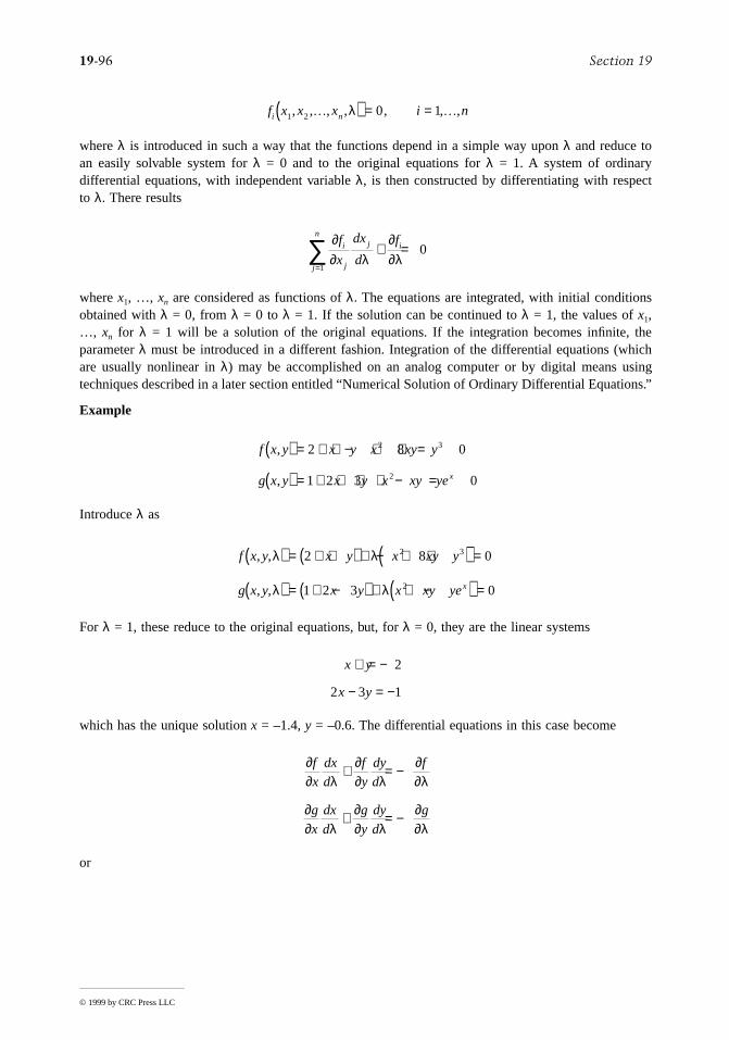
19-96 Section 19
© 1999 by CRC Press LLC
where λ is introduced in such a way that the functions depend in a simple way upon λ and reduce toan easily solvable system for λ = 0 and to the original equations for λ = 1. A system of ordinarydifferential equations, with independent variable λ, is then constructed by differentiating with respectto λ. There results
where x1, …, xn are considered as functions of λ. The equations are integrated, with initial conditionsobtained with λ = 0, from λ = 0 to λ = 1. If the solution can be continued to λ = 1, the values of x1,…, xn for λ = 1 will be a solution of the original equations. If the integration becomes infinite, theparameter λ must be introduced in a different fashion. Integration of the differential equations (whichare usually nonlinear in λ) may be accomplished on an analog computer or by digital means usingtechniques described in a later section entitled “Numerical Solution of Ordinary Differential Equations.”
Example
Introduce λ as
For λ = 1, these reduce to the original equations, but, for λ = 0, they are the linear systems
which has the unique solution x = –1.4, y = –0.6. The differential equations in this case become
or
f x x x i ni n1 2 0, , , , , , ,K Kλ( ) = = 1
∂∂ λ
∂∂λ
f
x
dx
d
fi
jj
nj i
=∑ + =
1
0
f x y x y x xy y
g x y x y x xy yex
,
,
( ) = + + − + + =
( ) = + + + + − =
2 8 0
1 2 3 0
2 3
2
f x y x y x xy y
g x y x y x xy yex
, ,
, ,
λ λ
λ λ
( ) = + +( ) + − + +( ) =
( ) = + −( ) + + −( ) =
2 8 0
1 2 3 0
2 3
2
x y
x y
+ = −
− = −
2
2 3 1
∂∂ λ
∂∂ λ
∂∂λ
∂∂ λ
∂∂ λ
∂∂λ
f
x
dx
d
f
y
dy
d
f
g
x
dx
d
g
y
dy
d
g
+ = −
+ = −

Mathematics 19-97
© 1999 by CRC Press LLC
Integrating in λ, with initial values x = –1.4 and y = –0.6 at λ = 0, from λ = 0 to λ = 1 gives the solution.
Interpolation and Finite Differences
The practicing engineer constantly finds it necessary to refer to tables as sources of information.Consequently, interpolation, or that procedure of “reading between the lines of the table,” is a necessarytopic in numerical analysis.
Linear Interpolation
If a function f(x) is approximately linear in a certain range, then the ratio [f(x1) – f(x0)]/(x1 – x0)= f[x0,x1] is approximately independent of x0 and x1 in the range. The linear approximation to the function f(x),x0 < x < x1, then leads to the interpolation formula
Divided Differences of Higher Order and Higher-Order Interpolation
The first-order divided difference f[x0, x1] was defined above. Divided differences of second and higherorder are defined iteratively by
and a convenient form for computational purposes is
for any k ≥ 0, where the ′ means the term (xj – xj) is omitted in the denominator. For example,
dx
d
f
y
g f g
xf
x
g
y
f
y
g
x
dy
d
f g
x
f
x
g
f
x
g
y
f
y
g
x
λ
∂∂
∂∂λ
∂∂λ
∂∂
∂∂
∂∂
∂∂
∂∂
λ
∂∂λ
∂∂
∂∂
∂∂λ
∂∂
∂∂
∂∂
∂∂
=−
−
=−
−
f x f x x x f x x f xx x
x xf x f x
x xx x f x x x f x
( ) ≈ ( ) + −( ) [ ] ≈ ( ) +−−
( ) − ( )[ ]
≈−
−( ) ( ) − −( ) ( )[ ]
0 0 0 1 00
1 01 0
1 01 0 0 1
1
,
f x x xf x x f x x
x x
f x x xf x x f x x x
x xkk k
k
0 1 21 2 0 1
2 0
0 11 0 1 1
0
, ,, ,
, , ,, , , , ,
[ ] = [ ] − [ ]−
[ ] = [ ] − [ ]−
−
M
KK K
f x x xf x
x x x x x xk
j
kj
j j j k
0 10
0 1
, , ,KL
[ ] =( )
−( ) −( ) −( )′∑=

19-98 Section 19
© 1999 by CRC Press LLC
If the accuracy afforded by a linear approximation is inadequate, a generally more accurate result maybe based upon the assumption that f(x) may be approximated by a polynomial of degree 2 or higherover certain ranges. This assumptions leads to Newton’s fundamental interpolation formula with divideddifferences:
where En(x) = error = [1/(n + 1)!]f(n–1) (ε)π(x) where min(x0, …, x) < ε < max(x0, x1,…, xn, x) and π(x)= (x – x0)(x – x1)…(x – xn). In order to use this most effectively, one may first form a divided-differencetable. For example, for third-order interpolation, the difference table is
where each entry is given by taking the difference between diagonally adjacent entries to the left, dividedby the abscissas corresponding to the ordinates intercepted by the diagonals passing through the calcu-lated entry.
Example. Calculate by third-order interpolation the value of cosh 0.83 given cosh 0.60, cosh 0.80,cosh 0.90, and cosh 1.10.
With n = 3, we have
which varies from the true value by 0.000 04.
Lagrange Interpolation Formulas
The Newton formulas are expressed in terms of divided differences. It is often useful to have interpolationformulas expressed explicitly in terms of the ordinates involved. This is accomplished by the Lagrangeinterpolation polynomial of degree n:
f x x xf x
x x x x
f x
x x x x
f x
x x x x0 1 20
0 1 0 2
1
1 0 1 2
2
2 0 2 1
, ,[ ] =( )
−( ) −( ) +( )
−( ) −( ) +( )
−( ) −( )
f x f x x x f x x x x x x f x x x
x x x x x x f x x x E xn n n
( ) ≈ ( ) + −( ) [ ] + −( ) −( ) [ ]+ −( ) −( ) −( ) [ ] + ( )−
0 0 0 1 0 1 0 1 2
0 1 1 0 1
, , ,
, , ,L K
x
x
x
x
f x
f x
f x
f x
f x x
f x x
f x x
f x x x
f x x xf x x x x
0
1
2
3
0
1
2
3
0 1
1 2
2 3
0 1 2
1 2 30 1 2 3
( )( )( )( )
[ ][ ][ ]
[ ][ ] [ ]
,
,
,
, ,
, ,, , ,
x
x
x
x
0
1
2
3
0 60
0 80
0 90
1 10
1 185 47
1 337 43
1 433 09
1 668 52
0 7598
0 9566
1 1772
0 6560
0 73530 1586
====
.
.
.
.
.
.
.
.
.
.
.
.
..
cosh . . . . . . .
. . . . .
0 83 1 185 47 0 23 0 7598 0 23 0 03 0 6560
0 23 0 03 0 07 0 1586 1 364 64
≈ + ( )( ) + ( )( )( )
+ ( )( ) −( )( ) =
y xx
x x xf x
j jj
n
j( ) = ( )−( ) ′( ) ( )
=∑ π
π0

Mathematics 19-99
© 1999 by CRC Press LLC
where
where (xj – xj) is the omitted factor. Thus,
Example. The interpolation polynomial of degree 3 is
Thus, directly from the data
we have as an interpolation polynomial y(x) for (x):
Other Difference Methods (Equally Spaced Ordinates)
Backward Differences.The backward differences denoted by
are useful for calculation near the end of tabulated data.
Central Differences.The central differences denoted by
x 0 1 3 4f(x) 1 1 –1 2
π
π
x x x x x x x
x x x x x x x
n
j j j j n
( ) = −( ) −( ) −( )′( ) = −( ) −( ) −( )
0 1
0 1
L
L
f x y x E xn( ) = ( ) + ( )
E xn
x fnn( ) =
+( ) ( ) ( )+( )11
1
!π ε
y xx x x x x x
x x x x x xf x
x x x x x x
x x x x x xf x
x x x x x x
x x
( ) =−( ) −( ) −( )−( ) −( ) −( ) ( ) +
−( ) −( ) −( )−( ) −( ) −( ) ( )
+−( ) −( ) −( )−
1 2 3
0 1 0 2 0 30
0 2 3
1 0 1 2 1 31
0 1 3
2 00 2 1 2 32
0 1 2
3 0 3 1 3 23( ) −( ) −( ) ( ) +
−( ) −( ) −( )−( ) −( ) −( ) ( )
x x x xf x
x x x x x x
x x x x x xf x
y xx x x x x x
x x x x x x
( ) = ⋅−( ) −( ) −( )−( ) −( ) −( )
+ ⋅−( ) −( )
−( ) −( ) −( )
− ⋅−( ) −( )
−( ) −( ) −( )+ ⋅
−( ) −( ) −( )−(
11 3 4
0 1 0 3 0 41
3 4
1 0 1 3 1 4
11 4
3 0 3 1 3 42
0 1 3
4 0)) −( ) −( )4 1 4 3
∇ ( ) = ( ) − −( )
∇ ( ) = ∇ ( ) − ∇ −( )
∇ ( ) = ∇ ( ) − ∇ −( )− −
f x f x f x h
f x f x f x h
f x f x f x hn n n
2
1 1
K

19-100 Section 19
© 1999 by CRC Press LLC
are useful for calculating at the interior points of tabulated data.Also to be found in the literature are Gaussian, Stirling, Bessel, Everett, Comrie differences, and so forth.
Inverse Interpolation
This is the process of finding the value of the independent variable or abscissa corresponding to a givenvalue of the function when the latter is between two tabulated values of the abscissa. One method ofaccomplishing this is to use Lagrange’s interpolation formula in the form
where x is expressed as a function of y. Other methods revolve about methods of iteration.
Numerical Differentiation
Numerical differentiation should be avoided wherever possible, particularly when data are empirical andsubject to appreciable observation errors. Errors in data can affect numerical derivatives quite strongly(i.e., differentiation is a roughening process). When such a calculation must be made, it is usuallydesirable first to smooth the data to a certain extent.
The Use of Interpolation Formulas
If the data are given over equidistant values of the independent variable x, an interpolation formula, suchas the Newton formula, may be used, and the resulting formula differentiated analytically. If theindependent variable is not at equidistant values, then Lagrange’s formulas must be used. By differen-tiating three- and five-point Lagrange interpolation formulas, the following differentiation formulas resultfor equally spaced tabular points.
Three-point Formulas.Let x0, x1, and x2 be the three points
where the last term is an error term and minj xj < ε < maxj xj.
Five-point Formulas.Let x0, x1, x2, x3, and x4 be the five values of the equally spaced independentvariable and fj = f(xj).
δ
δ δ δ
f x f xh
f xh
f x f xh
f xhn n n
( ) = +
− −
( ) = +
− −
− −
2 2
2 21 1
x yy
y y yx
j jj
n
j= ( ) = ( )−( ) ′( )=
∑ψπ
π0
′( ) = − ( ) + ( ) − ( )[ ] + ′′′( )
′( ) = − ( ) + ( )[ ] + ′′′( )
′( ) = ( ) − ( ) + ( )[ ] + ′′′
f xh
f x f x f xh
f
f xh
f x f xh
f
f xh
f x f x f xh
f
0 0 1 2
2
1 0 2
2
2 0 1 2
2
12
3 43
12 6
12
4 33
ε
ε
εε( )
′( ) = − + − + −[ ] + ( )( )f xh
f f f f fh
f v0 0 1 2 3 4
4112
25 48 36 16 35
ε

Mathematics 19-101
© 1999 by CRC Press LLC
and the last term is again an error term.
Smoothing Techniques
These techniques involve the approximation of the tabular data by a least squares fit of the data usingsome known functional form, usually a polynomial. In place of approximating f(x) by a single leastsquares polynomial of degree n over the entire range of the tabulation, it is often desirable to replaceeach tabulated value by the value taken on by a last squares polynomial of degree n relevant to a subrangeof 2M + 1 points centered, where possible, at the point for which the entry is to be modified. Thus, eachsmoothed value replaces a tabulated value. Let fi = f(xi) be the tabular points and yj = smoothed values.A first-degree least squares with three points would be
A first-degree least squares with five points would be
Thus, for example, if first-degree, five-point least squares are used, the central formula is used for allvalues except the first two and the last two, where the off-center formulas are used. A third-degree leastsquares with seven points would be
′( ) = − − + − +[ ] − ( )( )f xh
f f f f fh
f v1 0 1 2 3 4
4112
3 10 18 620
ε
′( ) = − + −[ ] + ( )( )f xh
f f f fh
f v2 0 1 3 4
4112
8 830
ε
′( ) = − + − + +[ ] − ( )( )f xh
f f f f fh
f v3 0 1 2 3 4
4112
6 18 10 320
ε
′( ) = − + − +[ ] + ( )( )f xh
f f f f fh
f v4 0 1 2 3 4
4112
3 16 36 48 255
ε
y f f f
y f f f
y f f f
016 0 1 2
113 0 1 2
216 0 1 2
5 2
2 5
= + −[ ]= + +[ ]= − + +[ ]
y f f f f
y f f f f
y f f f f f
y f f f f
y f f f f
015 0 1 2 4
11
10 0 1 2 3
215 0 1 2 3 4
31
10 0 1 2 3
415 0 2 3 4
3 2
4 3 2
2 3 4
2 3
= + + −[ ]= + + +[ ]= + + + +[ ]= + + +[ ]= − + + +[ ]

19-102 Section 19
© 1999 by CRC Press LLC
Additional smoothing formulas may be found in the references. After the data are smoothed, any of theinterpolation polynomials, or an appropriate least squares polynomial, may be fitted and the results usedto obtain the derivative.
Least Squares Method
Parabolic. For five evenly spaced neighboring abscissas labeled x–2, x–1, x0, x1, and x2, and their ordinatesf–2, f–1, f0, f1, and f2, assume a parabola is fit by least squares. There results for all interior points, exceptthe first and last two points of the data, the formula for the numerical derivative:
For the first two data points designated by 0 and h:
and for the last two given by α – h and α:
Quartic (Douglas-Avakian).A fourth-degree polynomial y = a + bx + cx2 + dx3 + ex4 is fitted to sevenadjacent equidistant points (spacing h) after a translation of coordinates has been made so that x = 0corresponds to the central point of the seven. Thus, these may be called –3h, –2h, –h, 0, h, 2h, and 3h.Let k = coefficient h for the seven points. This is, in –3h, k = –3. Then, the coefficients for the polynomialare
y f f f f f f f
y f f f f f f f
y f f f f f f f
y f f f
0142 0 1 2 3 4 5 6
1142 0 1 2 3 4 5 6
2142 0 1 2 3 4 5 6
3121 0 1
39 8 4 4 4 2
8 19 16 6 4 7 4
4 16 19 12 2 4
2 3 6
= + − − + + −[ ]= + + + − − +[ ]= − + + + + − +[ ]= − + + 22 3 4 5 6
4142 0 1 2 3 4 5 6
5142 0 1 2 3 4 5 6
6142 0 1 2 3 4 5
7 6 3 2
4 2 12 19 16 4
4 7 4 6 16 19 8
2 4 4 4 8 39
+ + + −[ ]= − + + + + −[ ]= − − + + + +[ ]= − + + − − + +
f f f f
y f f f f f f f
y f f f f f f f
y f f f f f f ff6[ ]
′ = − − + +[ ]− −fh
f f f f0 2 1 1 2
110
2 2
′( ) = − ( ) + ( ) + ( ) − ( )[ ]
′( ) = − ( ) + ( ) + ( ) + ( )[ ]
fh
f f h f h f h
f hh
f f h f h f h
01
2021 0 13 17 2 9 3
120
11 0 3 7 2 3
′ −( ) = − ( ) + −( ) + −( ) + −( )[ ]
′( ) = − ( ) + −( ) + −( ) − −( )[ ]
f hh
f f h f h f h
fh
f f h f h h
α α α α α
α α α α α
120
11 3 7 2 3
120
21 13 17 2 9 3

Mathematics 19-103
© 1999 by CRC Press LLC
where all summations run from k = –3 to k = +3 and f(kh) = tabular value at kh. The slope of thepolynomial at x = 0 is dy/dx = b.
Numerical Integration
Numerical evaluation of the finite integral f(x) dx is carried out by a variety of methods. A few aregiven here.
Newton-Cotes Formulas (Equally Spaced Ordinates)
Trapezoidal Rule.This formula consists of subdividing the interval a ≤ x ≤ b into n subintervals a to a+ h, a + h to a + 2h, …, and replacing the graph of f(x) by the result of joining the ends of adjacentordinates by line segments. If fj = f(xj) = f(a + jh), f0 = f(a), and fn = f(b), the integration formula is
where |En| = (nh3/12)|f ″(ε)| = [(b – a)3/12n2]|f ″(ε)|, a < ε < b. This procedure is not of high accuracy.However, if f ″(x) is continuous in a < x < b, the error goes to zero as l/n2, n → ∞.
Parabolic Rule (Simpson’s Rule).This procedure consists of subdividing the interval a < x < b into n/2subintervals, each of length 2h, where n is an even integer. Using the notation as above the integrationformula is
where
This method approximates f(x) by a parabola on each subinterval. This rule is generally more accuratethan the trapezoidal rule. It is the most widely used integration formula.
af kh k f kh k f kh
bkf kh
h
k f kh
h
cf kh k f kh k f kh
h
dkf kh k f kh
h
ef kh k f kh
=( ) − ( ) + ( )
=( )
−( )
=− ( ) + ( ) − ( )
=− ( ) + ( )
=( ) − ( )
∑ ∑ ∑
∑ ∑
∑ ∑ ∑
∑ ∑
∑ ∑
524 245 21
924
397
1512
7
216
840 679 67
3168
7
216
72 67
2 4
3
2 4
2
3
3
2 ++ ( )∑7
3168
4
4
k f kh
h
∫ ab
a
b
n n nf x dxh
f f f f f E∫ ( ) = + + + + +[ ] +−22 2 20 1 2 1L
a
b
n n n n nf x dxh
f f f f f f f f E∫ ( ) = + + + + + + + +[ ] +− − −34 2 4 4 2 40 1 2 3 3 2 1L
Enh
fb a
nf a bn
iv iv= ( ) =−( ) ( ) < <( ) ( )
5 3
4180 180ε ε ε

19-104 Section 19
© 1999 by CRC Press LLC
Weddle’s Rule.This procedure consists of subdividing the integral a < x < b into n/6 subintervals, eachof length 6h, where n is a multiple of 6. Using the notation from the trapezoidal rule, there results
Note that the coefficients of fj follow the rule 1, 5, 1, 6, 1, 5, 2, 5, 1, 6, 1, 5, 2, 5, etc.… This procedureconsists of approximately f(x) by a polynomial of degree 6 on each subinterval. Here,
Gaussian Integration Formulas (Unequally Spaced Abscissas)
These formulas are capable of yielding comparable accuracy with fewer ordinates than the equally spacedformulas. The ordinates are obtained by optimizing the distribution of the abscissas rather than byarbitrary choice. For the details of these formulas, Hildebrand (1956) is an excellent reference.
Two-Dimensional Formula
Formulas for two-way integration over a rectangle, circle, ellipse, and so forth, may be developed by adouble application of one-dimensional integration formulas. The two-dimensional generalization of theparabolic rule is given here. Consider the iterated integral f(x, y) dx dy. Subdivide c < x < d intom (even) subintervals of length h = (d – c)/m, and a < y < b into n (even) subintervals of length k = (b– a)/n. This gives a subdivision of the rectangle a ≤ y ≤ b and c ≤ x ≤ d into subrectangles. Let xj = c+ jh, yj = a + jk, and fi,j = f(xi, yj). Then,
where
where ε1 and ε2 lie in c < x < d, and η1 and η2 lie in a < y < b.
Numerical Solution of Ordinary Differential Equations
A number of methods have been devised to solve ordinary differential equations numerically. The generalreferences contain some information. A numerical solution of a differential equation means a table ofvalues of the function y and its derivatives over only a limited part of the range of the independentvariable. Every differential equation of order n can be rewritten as n first-order differential equations.Therefore, the methods given below will be for first-order equations, and the generalization to simulta-neous systems will be developed later.
The Modified Euler Method
This method is simple and yields modest accuracy. If extreme accuracy is desired, a more sophisticatedmethod should be selected. Let the first-order differential equation be dy/dx = f(x, y) with the initialcondition (x0, y0) (i.e., y = y0 when x = x0). The procedure is as follows.
a
b
n n n n nf x dxh
f f f f f f f f f f f f f E∫ ( ) = + + + + + + + + + + + + +[ ] +− − −310
5 6 5 2 5 6 50 1 2 3 4 5 6 7 8 3 2 1L
Enh
f h fn = ( ) + ( )[ ]( ) ( )7
61
2 821400
10 9ε ε
∫ ∫ab
cd
c
d
a
b
m m
m n n n
f x y dx dyhk
f f f f f f f f
f f f f f f f
∫∫ ( ) = + + + +( )[ + + + + +( )
+ + + + +( ) + + + + +
, , , , , , , , ,
, , , , , , ,
94 2 4 4 2
2 4 2 4 2
0 0 1 0 2 0 0 0 1 1 1 2 1 1
0 2 1 2 2 2 2 0 1 2
L L
L L LL +( )] +f Em n m n, ,
Ehk
mhf
xnk
f
ym n,
, ,= −
( )+
( )
90
44
1 14
44
2 24
∂ ε η∂
∂ ε η∂

Mathematics 19-105
© 1999 by CRC Press LLC
Step 1. From the given initial conditions (x0, y0) compute = f(x0, y0) and = [∂f(x0, y0)/∂x] +[∂f(x0, y0)/∂y] . Then, determine y1 = y0 + h + (h2/2) where h = subdivision of the independentvariable.
Step 2. Determine = f(x1, y1) where x1 = x0 + h. These prepare us for the following.
Predictor Steps.
Step 3. For n ≥ 1, calculate (yn+1)1 = yn–1 + 2hStep 4. Calculate = f[xn+1, (yn+1)1].
Corrector Steps.
Step 5. Calculate (yn+1)2 = yn + (h/2) where yn and without the subscripts are theprevious values obtained by this process (or by steps 1 and 2).
Step 6. = f[xn+1, (yn+1)2].Step 7. Repeat the corrector steps 5 and 6 if necessary until the desired accuracy is produced in yn+1,
Example. Consider the equation y′ = 2y2 + x with the initial conditions y0 = 1 when x0 = 0. Let h =0.1. A few steps of the computation are illustrated.
and so forth. This procedure. may be programmed for a computer. A discussion of the truncation errorof this process may be found in Milne (1953).
Modified Adam’s Method
The procedure given here was developed retaining third differences. It can then be considered as a moreexact predictor-corrector method than the Euler method. The procedure is as follows for dy/dx = f(x, y)and h = interval size.
Steps 1 and 2 are the same as in Euler method.
Predictor Steps.
Step 3. (yn+1)1 = yn + (h/24) etc…, are calculated instep 1.Step 4. = f[xn+1, (yn+1)1].
Step
1
2
3
4
5
6
5 (repeat)
6 (repeat)
′y0 ′′y0
′y0 ′y0 ′′y0 ,
′y1
′yn .( )′+yn 1 1
[( ) ],′ + ′+y yn n1 1 ′yn
( )′+yn 1 2
′+yn 1.
′ = + =y y x0 02
02 2
′′ = + ′ = + =y y y0 0 01 4 1 8 9
y121 0 1 2 0 1 2 9 1 245= + ( )( ) + ( )[ ] =. . .
′ = + = + =y y x1 12
12 3 100 0 1 3 200. . .
y y hy2 1 0 12 1 2 0 1 3 200 1 640( ) = + ′ = + ( ) =. . .
′( ) = ( ) + =y y x2 1 2 1
2
22 5 592.
y y y y2 2 1 2 1 10 1 2 1 685( ) = + ( ) ′( ) + ′[ ] =. .
′( ) = ( ) + =y y x2 2 2 2
2
22 5 878.
y y y y2 3 1 2 2 10 05 1 699( ) = + ( ) ′( ) + ′[ ] =. .
′( ) = ( ) + =y y x2 3 2 3
2
22 5 974.
[ ], , ,55 59 37 91 2 3 1′ − ′ + ′ − ′ ′ ′− − − −y y y y y yn n n n n n where
( )′+yn 1 1

19-106 Section 19
© 1999 by CRC Press LLC
Corrector Steps.
Step 5. (yn+1)2 = yn + (h/24)Step 6. = f[xn+1, (yn+1)2].Step 7. Iterate steps 5 and 6 if necessary.
Runge-Kutta Methods
These methods are self-starting and are inherently stable. Kopal (1955) is a good reference for theirderivation and discussion. Third- and fourth-order procedures are given below for dy/dx = f(x, y) and h= interval size.
For third-order (error ≈ h4).
and
for all n ≥ 0, with initial condition (x0, y0).For fourth-order (error ≈ h5),
and
Example. (Third-order) Let dy/dx = x – 2y, with initial condition y0 = 1 when x0 = 0, and let h = 0.1.Clearly, xn = nh. To calculate y1, proceed as follows:
[ ( ) ].9 19 51 1 1 2′ + ′ − ′ + ′+ − −y y y yn n n n
( )′+yn 1 2
k hf x y
k hf x h y k
k hf x h y k k
n n
n n
n n
0
11
21
2 0
2 1 02
= ( )= + +( )= + + −( )
,
,
,
y y k k kn n+ = + + +( )11
6 0 1 24
k hf x y
k hf x h y k
k hf x h y k
k hf x h y k
n n
n n
n n
n n
0
11
21
2 0
21
21
2 1
3 2
= ( )= + +( )= + +( )= + +( )
,
,
,
,
y y k k k kn n+ = + + + +( )11
6 0 1 2 32 2
k x y
k
k
y
0 0 0
1
2
11
6
0 1 2 0 2
0 1 0 05 2 1 0 1 0 175
0 1 0 1 2 1 0 35 0 2 0 16
1 0 2 0 7 0 16 0 8234
= −[ ] = −
= − −( )[ ] = −
= − − +( )[ ] = −
= + − − −( ) =
. .
. . . .
. . . . .
. . . .

Mathematics 19-107
© 1999 by CRC Press LLC
Equations of Higher Order and Simultaneous Differential Equations
Any differential equation of second- or higher order can be reduced to a simultaneous system of first-order equations by the introduction of auxiliary variables. Consider the following equations:
In the new variables x1 = x, x2 = y, x3 = z, x4 = dx1/dt, x5 = dx2/dt, and x6 = dx3/dt, the equations become
which is a system of the general form
where i = 1, 2, …, n. Such systems may be solved by simultaneous application of any of the abovenumerical techniques. A Runge-Kutta method for
is given below. The fourth-order procedure is shown.Starting at the initial conditions x0, y0, and t0, the next values x1 and y1 are computed via the equations
below (where ∆t = h, tj = h + tj–1):
d x
dtxy
dx
dtz e
d y
dtxy
dy
dtt
d z
dtxz
dz
dtx e
x
x
2
2
2
22
2
2
7
+ + =
+ = +
+ + =
dx
dtx
dx
dtx
dx
dtx
dx
dtx x x x e
dx
dtx x x t
dx
dtx x x x e
x
x
14
25
36
41 2 4 3
53 2 5
2
61 3 6 1
3
1
7
=
=
=
= − − +
= − + +
= − − +
dx
dtf t x x x xii n= ( ), , , , ,1 2 3 K
dx
dtf t x y
dy
dtg t x y
= ( )
= ( )
, ,
, ,
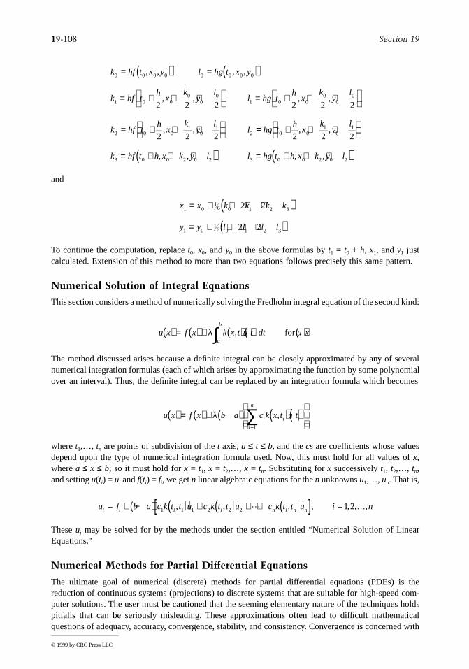
19-108 Section 19
© 1999 by CRC Press LLC
and
To continue the computation, replace t0, x0, and y0 in the above formulas by t1 = t0 + h, x1, and y1 justcalculated. Extension of this method to more than two equations follows precisely this same pattern.
Numerical Solution of Integral Equations
This section considers a method of numerically solving the Fredholm integral equation of the second kind:
The method discussed arises because a definite integral can be closely approximated by any of severalnumerical integration formulas (each of which arises by approximating the function by some polynomialover an interval). Thus, the definite integral can be replaced by an integration formula which becomes
where t1,…, tn are points of subdivision of the t axis, a ≤ t ≤ b, and the cs are coefficients whose valuesdepend upon the type of numerical integration formula used. Now, this must hold for all values of x,where a ≤ x ≤ b; so it must hold for x = t1, x = t2,…, x = tn. Substituting for x successively t1, t2,…, tn,and setting u(ti) = ui and f(ti) = fi, we get n linear algebraic equations for the n unknowns u1,…, un. That is,
These uj may be solved for by the methods under the section entitled “Numerical Solution of LinearEquations.”
Numerical Methods for Partial Differential Equations
The ultimate goal of numerical (discrete) methods for partial differential equations (PDEs) is thereduction of continuous systems (projections) to discrete systems that are suitable for high-speed com-puter solutions. The user must be cautioned that the seeming elementary nature of the techniques holdspitfalls that can be seriously misleading. These approximations often lead to difficult mathematicalquestions of adequacy, accuracy, convergence, stability, and consistency. Convergence is concerned with
k hf t x y l hg t x y
k hf th
xk
yl
l hg th
xk
yl
k hf th
xk
yl
l
0 0 0 0 0 0 0 0
1 0 00
00
1 0 00
00
2 0 01
01
2
2 2 2 2 2 2
2 2 2
= ( ) = ( )
= + + +
= + + +
= + + +
, , , ,
, , , ,
, , == + + +
= + + +( ) = + + +( )
hg th
xk
yl
k hf t h x k y l l hg t h x k y l
0 01
01
3 0 0 2 0 2 3 0 0 2 0 2
2 2 2, ,
, , , ,
x x k k k k
y y l l l l
1 01
6 0 1 2 3
1 01
6 0 1 2 3
2 2
2 2
= + + + +( )= + + + +( )
u x f x k x t u t dt u xa
b
( ) = ( ) + ( ) ( ) ( )∫λ , for
u x f x b a c k x t u ti i i
i
n
( ) = ( ) + −( ) ( ) ( )
=
∑λ ,1
u f b a c k t t u c k t t u c k t t u i ni i i i n i n n= + −( ) ( ) + ( ) + + ( )[ ] =1 1 1 2 2 2 1 2, , , , , , ,L K

Mathematics 19-109
© 1999 by CRC Press LLC
the approach of the approximate numerical solution to the exact solution as the number of mesh unitsincrease indefinitely in some sense. Unless the numerical method can be shown to converge to the exactsolution, the chosen method is unsatisfactory.
Stability deals in general with error growth in the calculation. As stated before, any numerical methodinvolves truncation and round-off errors. These errors are not serious unless they grow as the computationproceeds (i.e., the method is unstable).
Finite Difference Methods
In these methods, the derivatives are replaced by various finite differences. The methods will be illustratedfor problems in two space dimensions (x, y) or (x, t) where t is timelike. Using subdivisions ∆x = h and∆y = k with u(i h, jk) = ui,j, approximate ux|i,j = [(ui+1,j – ui,j)/h] + O(h) (forward difference), a first-order[O(h)] method, or ux|i,j = [(ui+1,j – ui–1,j)/2h] + O(h2) (central difference), a second-order method. Thesecond derivative is usually approximated with the second-order method [uxx|i,j = [(ui+1,j – 2ui,j + ui–1,j)/h2]+ O(h2)].
Example. Using second-order differences for uxx and uyy, the five-point difference equation (with h =k) for Laplace’s equation uxx + uyy = 0 is ui,j =1/4[ui+1,j + ui–1,j + ui,j+1 + ui,j–1]. The accuracy is O(h2). Thismodel is called implicit because one must solve for the total number of unknowns at the unknown gridpoints (i, j) in terms of the given boundary data. In this case, the system of equations is a linear system.
Example. Using a forward-difference approximation for ut and a second-order approximation for uxx,the diffusion equation ut = uxx is approximated by the explicit formula ui,j+1 = rui–1,j + (1 – 2r)ui,j + rui+1,j.This classic result permits step-by-step advancement in the t direction beginning with the initial data att = 0 (j = 0) and guided by the boundary data. Here, the term r = ∆t/(∆x)2 = k/h2 is restricted to be lessthan or equal to 1/2 for stability and the truncation error is O(k2 + kh2).
The Crank-Nicolson implicit formula which approximates the diffusion equation ut = uxx is
The stability of this numerical method was analyzed by Crandall (Ames, 1993) where the λ, r stabilitydiagram is given.
Approximation of the time derivative in ut = uxx by a central difference leads to an always unstableapproximation — the useless approximation
which is a warning to be careful.The foregoing method is symmetric with respect to the point (i, j), where the method is centered.
Asymmetric methods have some computational advantages, so the Saul’yev method is described (Ames,1993). The algorithms (r = k/h2)
are used as in any one of the following options:
1. Use Saul’yev A only and proceed line-by-line in the t(j) direction, but always from the leftboundary on a line.
2. Use Saul’yev B only and proceed line-by-line in the t(j) direction, but always from the rightboundary to the left on a line.
− + +( ) − = −( ) + − −( )[ ] + −( )− + + + + − +r u r u r u r u r u r ui j i j i j i j i j i jλ λ λ λ λ λ1 1 1 1 1 1 11 2 1 1 2 1 1, , , , , ,
u u r u u ui j i j i j i j i j, , , , ,+ − + −= + − +( )1 1 1 12 2
1
1
1 1 1 1
1 1 1 1
+( ) = + − +( ) ( )
+( ) = + − +( ) ( )
+ − + +
+ + + −
r u u r u u u
r u u r u u u
i j i j i j i j i j
i j i j i j i j i j
, , , , ,
, , , , ,
Saul' yev A
Saul' yev B
19-110 Section 19
© 1999 by CRC Press LLC
3. Alternate from line to line by first using Saul’yev A and then B, or the reverse. This is related toalternating direction methods.
4. Use Saul’yev A and Saul’yev B on the same line and average the results for the final answer (Afirst, and then B). This is equivalent to introducing the dummy variables Pi,j and Qi,j such that
and
This averaging method has some computational advantage because of the possibility of truncation errorcancellation. As an alternative, one can retain the Pi,j and Qi,j from the previous step and replace Ui,j andUi+1,j by Pi,j and Pi+1,j, respectively, and Ui,j and Ui–1,j by Qi,j and Qi–1,j, respectively.
Weighted Residual Methods (WRMs)
To set the stage for the method of finite elements, we briefly describe the WRMs, which have severalvariations — the interior, boundary, and mixed methods. Suppose the equation is Lu = f, where L is thepartial differential operator and f is a known function, of say x and y. The first step in WRM is to selecta class of known basis functions bi (e.g., trigonometric, Bessel, Legendre) to approximate u(x, y) as ~Σ ai bi (x, y) = U(x, y, a). Often, the bi are selected so that U(x, y, a) satisfy the boundary conditions.This is essentially the interior method. If the bi, in U(x, y, a) are selected to satisfy the differentialequations, but not the boundary conditions, the variant is called the boundary method. When neither theequation nor the boundary conditions are satisfied, the method is said to be mixed. The least ingenuityis required here. The usual method of choice is the interior method.
The second step is to select an optimal set of constants ai, i = 1,2, …, n, by using the residual RI(U)= LU – f. This is done here for the interior method. In the boundary method, there are a set of boundaryresidual RB, and, in the mixed method. Both RI and RB. Using the spatial average (w, v) = ∫vwvdV, thecriterion for selecting the values of ai is the requirement that the n spatial averages
These represent n equations (linear if the operator L is linear and nonlinear otherwise) for the ai.Particular WRMs differ because of the choice of the bjs. The most common follow.
1. Subdomain The domain V is divided into n smaller, not necessarily disjoint, subdomains Vj withwj(x, y) = 1 if (x, y) is in Vj, and 0 if (x, y) is not in Vj.
2. Collocation Select n points Pj = (xj, yj) in V with wj(Pj) = δ(P – Pj), where ∫vφ(P)δ(P – Pj)dP =φ(Pj) for all test functions φ(P) which vanish outside the compact set V. Thus, (wj, RE) = ∫vδ(P –Pj)REdV = RE[U(Pj) ≡ 0 (i.e., the residual is set equal to zero at the n points Pj).
3. Least squares Here, the functional I(a) = dV, where a = (a1, …, an), is to be made stationarywith respect to the aj. Thus, 0 = ∂I/∂aj = 2∫vRE(∂RE/∂aj)dV, with j = 1, 2, …, n. The wj in this caseare ∂RE/∂aj.
4. Bubnov-Galerkin Choose wj(P) = bj(P). This is perhaps the best-known method.5. Stationary Functional (Variational) Method With φ a variational integral (or other functional), set
∂φ[U]/∂aj = 0, where j = 1, …, n, to generate the n algebraic equations.
1
1
1 1 1 1
1 1 1 1
+( ) = + − +( )+( ) = + − +( )
+ − + +
+ + + −
r P U r P U U
r Q U r Q U U
i j i j i j i j i j
i j i j i j i j i j
, , , , ,
, , , , ,
U P Qi j i j i j, , ,+ + += +( )112 1 1
b R U i ni E, , , , ,( )( ) = =0 1 2 K
∫V ER2

Mathematics 19-111
© 1999 by CRC Press LLC
Example. uxx + uyy = –2, with u = 0 on the boundaries of the square x = ±1, y = ±1. Select an interiormethod with U = a1(1 – x2)(1 – y2) + a2x2y2(1 – x2)(1 – y2), whereupon the residual RE(U) = 2a1(2 – x2
– y2) + 2a2[(1 – 6x2)y2(1 – y2) + (1 – 6y2) – (1 – x2)] + 2. Collocating at (1/3, 1/3) and (2/3, 2/3) givesthe two linear equations –32a1/9 + 32a2/243x2 + 2 = 0 and –20a1/9 – 400a2/243 + 2 = 0 for a1 and a2.
WRM methods can obviously be used as approximate methods. We have now set the stage for finiteelements.
Finite Elements
The WRM methods are more general than the finite elements (FE) methods. FE methods require, inaddition, that the basis functions be finite elements (i.e., functions that are zero except on a small partof the domain under consideration). A typical example of an often used basis is that of triangular elements.For a triangular element with Cartesian coordinates (x1, y1), (x2, y2), and (x3, y3), define natural coordinatesL1, L2, and L3 (Li, ↔ (xi, yi)) so that Li = Ai/A where
is the area of the triangle and
Clearly L1 + L2 + L3 = 1, and the Li are one at node i and zero at the other nodes. In terms of the Cartesiancoordinates,
is the linear triangular element relation.Tables of linear, quadratic, and cubic basis functions are given in the literature. Notice that while the
linear basis needs three nodes, the quadratic requires six and the cubic basis ten. Various modifications,such as the Hermite basis, are described in the literature. Triangular elements are useful in approximatingirregular domains.
For rectangular elements, the chapeau functions are often used. Let us illustrate with an example. Letuxx + uyy = Q, 0 < x < 2, 0 < y < 2, u(x, 2) = 1, u(0, y) = 1, uy(x, 0) = 0, ux(2, y) = 0, and Q(x, y) =Qwδ(x – 1)δ(y – 1),
A
x y
x y
x y
=
12
1 1
2 2
3 3
1
1
1
det
A
x y
x y
x y
A
x y
x y
x y
A
x y
x y
x y
112 2 2
3 3
212
1 1
3 3
312
1 1
2 2
1
1
1
1
1
1
1
1
1
=
=
=
det
det
det
L
L
LA
x y x y y y x x
x y x y y y x x
x y x y y y x x
x
y
1
2
3
2 3 3 2 2 3 3 2
3 1 1 3 3 1 1 3
1 2 2 1 1 2 2 1
12
1
=− − −− − −− − −
, ,
, ,
, ,

19-112 Section 19
© 1999 by CRC Press LLC
Using four equal rectangular elements, map the element I with vertices at (0, 0) (0, 1), (1, 1), and (1,0) into the local (canonical) coordinates (ξ, η), – 1 ≤ ξ ≤ 1, – 1 ≤ η ≤ 1, by means of x = 1/2(ξ + 1), y= 1/2(η + 1). This mapping permits one to develop software that standardizes the treatment of allelements. Converting to (ξ, η) coordinates, our problem becomes uξξ + uηη = 1/4Q, – 1 ≤ ξ ≤ 1, – 1 ≤η ≤ 1, Q = Qwδ(ξ – 1)δ(η – 1).
First, a trial function (ξ, η) is defined as u(ξ, η) ≈ (ξ, η) = Ajφj(ξ, η) (in element I) wherethe φj are the two-dimensional chapeau functions
Clearly φi take the value one at node i, provide a bilinear approximation, and are nonzero only overelements adjacent to node i.
Second, the equation residual RE = ∇ 2 – 1/4Q is formed and a WRM procedure is selected toformulate the algebraic equations for the Ai. This is indicated using the Galerkin method. Thus, forelement I, we have
Applying Green’s theorem, this result becomes
Using the same procedure in all four elements and recalling the property that the φi in each element arenonzero only over elements adjacent to node i gives the following nine equations:
where the cξ and cη are the direction cosines of the appropriate element (e) boundary.
Method of Lines
The method of lines, when used on PDEs in two dimensions, reduces the PDE to a system of ordinarydifferential equations (ODEs), usually by finite difference or finite element techniques. If the originalproblem is an initial value (boundary value) problem, then the resulting ODEs form an initial value(boundary value) problem. These ODEs are solved by ODE numerical methods.
δ xx
x( ) =
≠=
0 0
1 0
u µ Σ j=14
φ ξ η φ ξ η
φ ξ η φ ξ η
112
12 2
12
12
312
12 4
12
12
1 1 1 1
1 1 1 1
= −( ) −( )[ ] = +( ) −( )[ ]= +( ) +( )[ ] = −( ) +( )[ ]
u
u u Q d d i
D
i
I
ξξ ηη φ ξ η ξ η+ −( ) ( ) = =∫∫ , , , ,0 1 4K
u u Q d d u c u c ds ii i i
DD
i
II
ξ ξ η η ξ ξ η η∂
φ φ φ ξ η φ( ) + ( ) +[ ] − +( ) = =∫∫ ∫14 0 1 2 4, , , ,K
A Q d d
u c u c ds n
j j i j i
jD
i
e
De
e
e
φ φ φ φ φ ξ η
φ
ξ ξ η η
ξ ξ η η∂
( ) ( ) + ( ) ( )
+
− +( ) = =
==
=
∑∫∫∑
∫∑
1
9
14
1
1
0 1 2 9
4
4
, , , ,K

Mathematics 19-113
© 1999 by CRC Press LLC
Example. ut = uxx + u2, 0 < x < 1, 0 < t, with the initial value u(x, 0) = x, and boundary data u(0, t) =0, u(1, t) = sin t. A discretization of the space variable (x) is introduced and the time variable is leftcontinuous. The approximation is = (ui+1 – 2ui + ui–1)/h2 + With h = 1/5, the equations become
and u1(0) = 0.2, u2(0) = 0.4, u3(0) = 0.6, and u4(0) = 0.8.
Discrete and Fast Fourier Transforms
Let x(n) be a sequence that is nonzero only for a finite number of samples in the interval 0 ≤ n ≤ N –1. The quantity
is called the discrete Fourier transform (DFT) of the sequence x(n). Its inverse (IDFT) is given by
Clearly, DFT and IDFT are finite sums and there are N frequency values. Also, X(k) is periodic in kwith period N.
Example. x(0) = 1, x(1) = 2, x(2) = 3, x(3) = 4
Thus,
and X(1) = x(0) + x(1)e–iπ/2 + x(2)e–iπ + x(3)e–i3π/2 = 1 – 2i – 3 + 4i = – 2 + 2i; X(2) = –2; X(3) = –2 – 2i.
DFT Properties
1. Linearity: If x3(n) = ax1(n) + bx2(n), then X3(k) = aX1(k) + bX2(k).2. Symmetry: For x(n) real, Re[X(k)] = Re[X(N – k)], Im[(k)] = –Im[X(N – k)].
ui ui2 .
u t
u u u u
u u u u u
u u u u u
u t u u u
u t
0
1125 2 1 1
2
2125 3 2 1 2
2
3125 4 3 2 3
2
4125 4 3 4
2
5
0
2
2
2
2
( ) =
= −[ ] +
= − +[ ] +
= − +[ ] +
= − +[ ] +
=
˙
˙
˙
˙ sin
sin
X k x n e k Ni N nk
n
N
( ) = ( ) = −− ( )
=
−
∑ 2
0
1
0 1 1π , , , ,K
x nN
X k e n N ii N nk
k
N
( ) = ( ) = − = −( )( )
=
−
∑10 1 1 12
0
12π , , , ,K
X k x n e ki nk
n
( ) = ( ) =− ( )
=∑ 2 4
0
3π , 0, 1, 2, 3, 4
X x nn
0 100
3
( ) = ( ) ==
∑

19-114 Section 19
© 1999 by CRC Press LLC
3. Circular shift: By a circular shift of a sequence defined in the interval 0 ≤ n ≤ N – 1, we meanthat, as values fall off from one end of the sequence, they are appended to the other end. Denotingthis by x(n ⊕ m), we see that positive m means shift left and negative m means shift right. Thus,x2(n) = x1(n ⊕ m) ⇔ X2(k) = X1(k)ei(2π/N)km.
4. Duality: x(n) ⇔ X(k) implies (1/N)X(n) ⇔ x(–k).5. Z-transform relation: X(k) = k = 0,1, …, N – 1.6. Circular convolution: x3(n) = x1(m)x2(n * m) = x1(n * ,)x2(,) where x2(n * m)
corresponds to a circular shift to the right for positive m.
One fast algorithm for calculating DFTs is the radix-2 fast Fourier transform developed by J. W. Cooleyand J. W. Tucker. Consider the two-point DFT X(k) = x(n)e–i(2π/2)nk, k = 0, 1. Clearly, X(k) =x(0) + x(1)e–iπk. So, X(0) = x(0) + x(1) and X(1) = x(0) – x(1). This process can be extended toDFTs of length N = 2r, where r is a positive integer. For N = 2r, decompose the N-point DFT intotwo N/2-point DFTs. Then, decompose each N/2-point DFT into two N/4-point DFTs, and so onuntil eventually we have N/2 two-point DFTs. Computing these as indicated above, we combinethem into N/4 four-point DFTs and then N/8 eight-point DFTs, and so on, until the DFT iscomputed. The total number of DFT operations (for large N) is O(N2), and that of the FFT is O(Nlog2 N), quite a saving for large N.
Figure 19.12.1
Figure 19.12.2 Figure 19.12.3
FIGURES 19.12.1 to 19.12.3 The “Oregonator” is a periodic chemical reaction describable by three nonlinear first-order differential equations. The results (Figure 19.12.1) illustrate the periodic nature of the major chemical versustime. Figure 19.12.2 shows the phase diagram of two of the reactants, and Figure 19.12.3 is the three-dimensionalphase diagram of all reactants. The numerical computation was done using a fourth-order Runge-Kuta method onMathematica by Waltraud Rufeger at the Georgia Institute of Technology.
X zz ei k N( )| ,( / )= 2π
ΣmN
=−
01
Σ l=−01N
Σn=01

Mathematics 19-115
© 1999 by CRC Press LLC
Software
Some available software is listed here.
General Packages
General software packages include Maple, Mathematica, and Matlab. All contain algorithms for handlinga large variety of both numerical and symbolic computations.
Special Packages for Linear Systems
In the IMSL Library, there are three complementary linear system packages of note.LINPACK is a collection of programs concerned with direct methods for general (or full) symmetric,
symmetric positive definite, triangular, and tridiagonal matrices. There are also programs for least squaresproblems, along with the QR algorithm for eigensystems and the singular value decompositions ofrectangular matrices. The programs are intended to be completely machine independent, fully portable,and run with good efficiency in most computing environments. The LINPACK User’s Guide by Dongarraet al. is the basic reference.
ITPACK is a modular set of programs for iterative methods. The package is oriented toward the sparsematrices that arise in the solution of PDEs and other applications. While the programs apply to fullmatrices, that is rarely profitable. Four basic iteration methods and two convergence acceleration methodsare in the package. There is a Jacobi, SOR (with optimum relaxation parameter estimated), symmetricSOR, and reduced system (red-black ordering) iteration, each with semi-iteration and conjugate gradientacceleration. All parameters for these iterations are automatically estimated. The practical and theoreticalbackground for ITPACK is found in Hagemen and Young (1981).
YALEPACK is a substantial collection of programs for sparse matrix computations.
Ordinary Differential Equations Packages
Also in IMSL, one finds such sophisticated software as DVERK, DGEAR, or DREBS for initial valueproblems. For two-point boundary value problems, one finds DTPTB (use of DVERK and multipleshooting) or DVCPR.
Partial Differential Equations Packages
DISPL was developed and written at Argonne National Laboratory. DISPL is designed for nonlinearsecond-order PDEs (parabolic, elliptic, hyperbolic (some cases), and parabolic-elliptic). Boundary con-ditions of a general nature and material interfaces are allowed. The spatial dimension can be either oneor two and in Cartesian, cylindrical, or spherical (one dimension only) geometry. The PDEs are reducedto ordinary DEs by Galerkin discretization of the spatial variables. The resulting ordinary DEs in thetimelike variable are then solved by an ODE software package (such as GEAR). Software featuresinclude graphics capabilities, printed output, dump/restart/facilities, and free format input. DISPL isintended to be an engineering and scientific tool and is not a finely tuned production code for a smallset of problems. DISPL makes no effort to control the spatial discretization errors. It has been used tosuccessfully solve a variety of problems in chemical transport, heat and mass transfer, pipe flow, etc.
PDELIB was developed and written at Los Alamos Scientific Laboratory. PDELIB is a library ofsubroutines to support the numerical solution of evolution equations with a timelike variable and oneor two space variables. The routines are grouped into a dozen independent modules according to theirfunction (i.e., accepting initial data, approximating spatial derivatives, advancing the solution in time).Each task is isolated in a distinct module. Within a module, the basic task is further refined into general-purpose flexible lower-level routines. PDELIB can be understood and used at different levels. Within asmall period of time, a large class of problems can be solved by a novice. Moreover, it can provide awide variety of outputs.
DSS/2 is a differential systems simulator developed at Lehigh University as a transportable numericalmethod of lines (NMOL) code. See also LEANS.
FORSIM is designed for the automated solution of sets of implicitly coupled PDEs of the form
19-116 Section 19
© 1999 by CRC Press LLC
The user specifies the φi in a simple FORTRAN subroutine. Finite difference formulas of any order maybe selected for the spatial discretization and the spatial grid need not be equidistant. The resulting systemof time-dependent ODEs is solved by the method of lines.
SLDGL is a program package for the self-adaptive solution of nonlinear systems of elliptic andparabolic PDEs in up to three space dimensions. Variable step size and variable order are permitted. Thediscretization error is estimated and used for the determination of the optimum grid and optimum orders.This is the most general of the codes described here (not for hyperbolic systems, of course). This packagehas seen extensive use in Europe.
FIDISOL (finite difference solver) is a program package for nonlinear systems of two-or three-dimensional elliptic and parabolic systems in rectangular domains or in domains that can be transformedanalytically to rectangular domains. This package is actually a redesign of parts of SLDGL, primarilyfor the solution of large problems on vector computers. It has been tested on the CYBER 205, CRAY-IM, CRAY X-MP/22, and VP 200. The program vectorizes very well and uses the vector arithmeticefficiently. In addition to the numerical solution, a reliable error estimate is computed.
CAVE is a program package for conduction analysis via eigenvalues for three-dimensional geometriesusing the method of lines. In many problems, much time is saved because only a few terms suffice.
Many industrial and university computing services subscribe to the IMSL Software Library. Announce-ments of new software appear in Directions, a publication of IMSL. A brief description of some IMSLpackages applicable to PDEs and associated problems is now given. In addition to those packages justdescribed, two additional software packages bear mention. The first of these, the ELLPACK system,solves elliptic problems in two dimensions with general domains and in three dimensions with box-shaped domains. The system contains over 30 numerical methods modules, thereby providing a meansof evaluating and comparing different methods for solving elliptic problems. ELLPACK has a specialhigh-level language making it easy to use. New algorithms can be added or deleted from the systemwith ease.
Second, TWODEPEP is IMSL’s general finite element system for two-dimensional elliptic, parabolic,and eigenvalue problems. The Galerkin finite elements available are triangles with quadratic, cubic, orquartic basic functions, with one edge curved when adjacent to a curved boundary, according to theisoparametric method. Nonlinear equatons are solved by Newton’s method, with the resulting linearsystem solved directly by Gauss elimination. PDE/PROTRAN is also available. It uses triangularelements with piecewise polynomials of degree 2, 3, or 4 to solve quite general steady state, time-dependent, and eigenvalue problems in general two-dimensional regions. There is a simple user input.Additional information may be obtained from IMSL. NASTRAN and STRUDL are two advanced finiteelement computer systems available from a variety of sources. Another, UNAFEM, has been extensivelyused.
References
General
Adams, E. and Kulisch, U. (Eds.) 1993. Scientific Computing with Automatic Result Verification, Aca-demic Press, Boton, MA.
Gerald, C. F. and Wheatley, P. O. 1984. Applied Numerical Analysis, Addison-Wesley, Reading, MA.Hamming, R. W. 1962. Numerical Methods for Scientists and Engineers, McGraw-Hill, New York.Hildebrand, F. B. 1956. Introduction to Numerical Analysis, McGraw-Hill, New York.Isaacson, E. and Keller, H. B. 1966. Analysis of Numerical Methods, John Wiley & Sons, New York.Kopal, Z. 1955. Numerical Analysis, John Wiley & Sons, New York.Rice, J. R. 1993. Numerical Methods, Software and Analysis, 2nd ed. Academic Press, Boston, MA.Stoer, J. and Bulirsch, R. 1976. Introduction to Numerical Analysis, Springer, New York.
∂∂
φu
tx t u u u u u i Ni
i i j i x i xx j xx= ( ) ( ) ( )( ) =, , , , , , , , , , , ,K K K Kfor 1

Mathematics 19-117
© 1999 by CRC Press LLC
Linear Equations
Bodewig, E. 1956. Matrix Calculus, Wiley (Interscience), New York.Hageman, L. A. and Young, D. M. 1981. Applied Iterative Methods, Academic Press, Boston, MA.Varga, R. S. 1962. Matrix Iterative Numerical Analysis, John Wiley & Sons, New York.Young, D. M. 1971. Iterative Solution of Large-Linear Systems, Academic Press, Boston, MA.
Ordinary Differential Equations
Aiken, R. C. 1985. Stiff Computation, Oxford Unitersity Press, New York.Gear, C. W. 1971. Numerical Initial Value Problems in Ordinary Differential Equations, Prentice Hall,
Englewood Cliffs, NJ.Keller, H. B. 1976. Numerical Solutions of Two Point Boundary Value Problems, SIAM, Philadelphia, PA.Lambert, J. D. 1973. Computational Methods in Ordinary Differential Equations, Cambridge University
Press, New York.Milne, W.E. 1953. Numerical Solution of Differential Equations, John Wiley & Sons, New York.Rickey, K. C., Evans, H. R., Griffiths, D. W., and Nethercot, D. A. 1983. The Finite Element Method
— A Basic Introduction for Engineers, 2nd ed. Halstead Press, New York.Shampine, L. and Gear, C. W. 1979. A User’s View of Solving Stiff Ordinary Differential Equatons,
SIAM Rev. 21:1–17.
Partial Differential Equations
Ames, W. F. 1993. Numerical Methods for Partial Differential Equations, 3d ed. Academic Press, Boston,MA.
Brebbia, C. A. 1984. Boundary Element Techniques in Computer Aided Engineering, Martinus Nijhoff,Boston, MA.
Burnett, D. S. 1987. Finite Element Analysis, Addison-Wesley, Reading, MA.Lapidus, L. and Pinder, G. F. 1982. Numerical Solution of Partial Differential Equations in Science and
Engineering, John Wiley & Sons, New York.Roache, P. 1972. Computational Fluid Dynamics, Hermosa, Albuquerque, NM.
19-118 Section 19
© 1999 by CRC Press LLC
19.13 Experimental Uncertainty Analysis
W.G. Steele and H.W. Coleman
Introduction
The goal of an experiment is to answer a question by measuring a specific variable, Xi, or by determininga result, r, from a functional relationship among measured variables
(19.13.1)
In all experiments there is some error that prevents the measurement of the true value of each variable,and therefore, prevents the determination of r true.
Uncertainty analysis is a technique that is used to estimate the interval about a measured variable ora determined result within which the true value is thought to lie with a certain degree of confidence. Asdiscussed by Coleman and Steele (1989), uncertainty analysis is an extremely useful tool for all phasesof an experimental program from initial planning (general uncertainty analysis) to detailed design,debugging, test operation, and data analysis (detailed uncertainty analysis).
The application of uncertainty analysis in engineering has evolved considerably since the classic paperof Kline and McClintock (1953). Developments in the field have been especially rapid and significantover the past decade, with the methods formulated by Abernethy and co-workers (1985) that wereincorporated into ANSI/ASME Standards in (1984) and (1986) being superseded by the more rigorousapproach presented in the International Organization for Standardization (ISO) Guide to the Expressionof Uncertainty in Measurement (1993). This guide, published in the name of ISO and six other interna-tional organizations, has in everything but name established a new international experimental uncertaintystandard.
The approach in the ISO Guide deals with “Type A” and “Type B” categories of uncertainties, notthe more traditional engineering categories of systematic (bias) and precision (random) uncertainties,and is of sufficient complexity that its application in normal engineering practice is unlikely. This issuehas been addressed by AGARD Working Group 15 on Quality Assessment for Wind Tunnel Testing, bythe Standards Subcommittee of the AIAA Ground Test Technical Committee, and by the ASME Com-mittee PTC 19.1 that is revising the ANSI/ASME Standard (1986). The documents issued by two ofthese groups (AGARD-AR-304, 1994) and (AIAA Standard S-071-1995, 1995) and in preparation bythe ASME Committee present and discuss the additional assumptions necessary to achieve a less complex“large sample” methodology that is consistent with the ISO Guide, that is applicable to the vast majorityof engineering testing, including most single-sample tests, and that retains the use of the traditionalengineering concepts of systematic and precision uncertainties. The range of validity of this “largesample” approximation has been presented by Steele et al. (1994) and by Coleman and Steele (1995).The authors of this section are also preparing a second edition of Coleman and Steele (1989), whichwill incorporate the ISO Guide methodology and will illustrate its use in all aspects of engineeringexperimentation.
In the following, the uncertainties of individual measured variables and of determined results arediscussed. This section concludes with an overview of the use of uncertainty analysis in all phases ofan experimental program.
Uncertainty of a Measured Variable
For a measured variable, Xi, the total error is caused by both precision (random) and systematic (bias)errors. This relationship is shown in Figure 19.13.1. The possible measurement values of the variableare scattered in a distribution (here assumed Gaussian) around the parent population mean, µi. The parentpopulation mean differs from (Xi,)true by an amount called the systematic (or bias) error, βi. The quantity
r r X X X Xi J= 1 2, , , , ,K K( )

Mathematics 19-119
© 1999 by CRC Press LLC
βi is the total fixed error that remains in the measurement process after all calibration corrections havebeen made. In general, there will be several sources of bias error such as calibration standard errors,data acquisition errors, data reduction errors, and test technique errors. There is usually no direct wayto measure these errors, so they must be estimated.
For each bias error source, (βi)k, the experimenter must estimate a systematic uncertainty (or biaslimit), (B i)k, such that there is about a 95% confidence that (Bi)k ≥ |(βi)k|. Systematic uncertainties areusually estimated from previous experience, calibration data, analytical models, and the application ofsound engineering judgment. For each variable, there will be a set, Ki, of elemental systematic uncer-tainties, (Bi)k, for the significant fixed error sources. The overall systematic uncertainty for variable Xi
is determined from these estimates as
(19.13.2)
For a discussion on estimating systematic uncertainties (bias limits), see Coleman and Steele (1989).The estimate of the precision error for a variable is the sample standard deviation, or the estimate of
the error associated with the repeatability of a particular measurement. Unlike the systematic error, theprecision error varies from reading to reading. As the number of readings, Ni, of a particular variabletends to infinity, the distribution of these readings becomes Gaussian.
The readings used to calculate the sample standard deviation for each variable must be taken overthe time frame and conditions which cover the variation in the variable. For example, taking multiplesamples of data as a function of time while holding all other conditions constant will identify the randomvariation associated with the measurement system and the unsteadiness of the test condition. If thesample standard deviation of the variable being measured is also expected to be representative of otherpossible variations in the measurement, e.g., repeatability of test conditions, variation in test configura-tion, then these additional error sources will have to be varied while the multiple data samples are takento determine the standard deviation.
When the value of a variable is determined as the mean, of Ni readings, then the sample standarddeviation of the mean is
(19.13.3)
FIGURE 19.13.1 Errors in the measurement of variable Xi.
B Bi i kk
Ki
2 2
1
= ( )=
∑
Xi ,
SN N
X XX
i ii k i
k
N
i
i
=−( )
( ) −[ ]
=∑1
1
2
1
1 2
19-120 Section 19
© 1999 by CRC Press LLC
where
(19.13.4)
It must be stressed that these Ni readings have to be taken over the appropriate range of variations forXi as described above.
When only a single reading of a variable is available so that the value used for the variable is Xi, then previous readings, (XPi)k, must be used to find the standard deviation for the variable as
(19.13.5)
where
(19.13.6)
Another situation where previous readings of a variable are useful is when a small current samplesize, Ni, is used to calculate the mean value, of a variable. If a much larger set of previous readingsfor the same test conditions is available, then it can be used to calculate a more appropriate standarddeviation for the variable (Steele et al., 1993) as
(19.13.7)
where Ni is the number of current readings averaged to determine and is computed from previous readings using Equation (19.13.5). Typically, these larger data sets are taken in the early “shake-down” or “debugging” phases of an experimental program.
For many engineering applications, the “large sample” approximation applies, and the uncertainty forvariable i (Xi or is
(19.13.8)
where Si is found from the applicable Equation (19.13.3), (19.13.5) or (19.13.7). The interval Xi ± Ui or + Ui, as appropriate, should contain (Xi)true 95 times out of 100. If a small number of samples (Ni
or < 10) is used to determine or , then the “large sample” approximation may not applyand the methods in ISO (1993) or Coleman and Steele (1995) should be used to find Ui.
Uncertainty of a Result
Consider an experimental result that is determined for J measured variables as
X
X
Ni
i kk
N
i
i
=( )
=∑
1
NPi
SN
X XXPi
Pk
P
k
N
i i i
Pi
=− ( ) −
=∑1
1
2
1
1 2
XN
XPP
Pk
k
N
i
i
i
Pi
= ( )=
∑1
1
Xi ,
SS
NX
X
ii
i=
Xi , SXiNPi
Xi )
U B Si i i= + ( )2 22
Xi
NPiS
XiSXi
r r X X X Xi J= 1 2, , , , ,K K( )

Mathematics 19-121
© 1999 by CRC Press LLC
where some variables may be single readings and others may be mean values. A typical mechanicalengineering experiment would be the determination of the heat transfer in a heat exchanger as
(19.13.9)
where q is the heat rate, is the flow rate, cp is the fluid specific heat, and To and Ti are the heatedfluid outlet and inlet temperatures, respectively. For the “large sample” approximation, Ur is found as
(19.13.10)
where Br is the systematic uncertainty of the result
(19.13.11)
with
(19.13.12)
and Sr is the standard deviation of the result
(19.13.13)
The term Bik in Equation (19.13.11) is the covariance of the systematic uncertainties. When theelemental systematic uncertainties for two separately measured variables are related, for instance whenthe transducers used to measure different variables are each calibrated against the same standard, thesystematic uncertainties are said to be correlated and the covariance of the systematic errors is nonzero.The significance of correlated systematic uncertainties is that they can have the effect of either decreasingor increasing the uncertainty in the result. Bik is determined by summing the products of the elementalsystematic uncertainties for variables i and k that arise from the same source and are therefore perfectlycorrelated (Brown et al., 1996) as
(19.13.14)
where L is the number of elemental systematic error sources that are common for measurements Xi and Xk.If, for example,
(19.13.15)
and it is possible for portions of the systematic uncertainties B1 and B2 to arise from the same source(s),Equation (19.13.11) gives
(19.13.16)
q mc T Tp o i= −( )˙
m
U B Sr r r= + ( )2 22
B B Br i i
i
J
i k ik
k i
J
i
J2 2
1 11
1
2= ( ) += = +=
−
∑ ∑∑θ θ θ
θ ∂∂i
i
r
X=
S Sr i i
i
J2 2
1
= ( )=
∑ θ
B B Bik i
L
k= ( ) ( )=
∑ αα
α1
r r X X= ( )1 2,
B B B Br2
12
12
22
22
1 2 122= + +θ θ θ θ
19-122 Section 19
© 1999 by CRC Press LLC
For a case in which the measurements of X1 and X2 are each influenced by four elemental systematicerror sources and sources two and three are the same for both X1 and X2, Equation (19.13.2) gives
(19.13.17)
and
(19.13.18)
while Equation (19.13.14) gives
(19.13.19)
In the general case, there would be additional terms in the expression for the standard deviation ofthe result, Sr , (Equation 19.13.13) to take into account the possibility of precision errors in differentvariables being correlated. These terms have traditionally been neglected, although precision errors indifferent variables caused by the same uncontrolled factor(s) are certainly possible and can have asubstantial impact on the value of Sr (Hudson et al., 1996). In such cases, one would need to acquiresufficient data to allow a valid estimate of the precision covariance terms using standard statisticaltechniques (ISO, 1993). Note, however, that if multiple test results over an appropriate time period areavailable, these can be used to directly determine Sr . This value of the standard deviation of the resultimplicitly includes the correlated error effect.
If a test is performed so that M multiple sets of measurements (X1, X2, …, XJ)k at the same testcondition are obtained, then M results can be determined using Equation (19.13.1) and a mean result,
can be determined using
(19.13.20)
The standard deviation of the sample of M results, Sr , is calculated as
(19.13.21)
The uncertainty associated with the mean result, for the “large sample” approximation is then
(19.13.22)
where
(19.13.23)
and where Br is given by Equation (19.13.11).The “large sample” approximation for the uncertainty of a determined result (Equations (19.13.10)
or (19.13.22)) applies for most engineering applications even when some of the variables have fewer
B B B B B12
1 1
2
1 2
2
1 3
2
1 4
2= ( ) + ( ) + ( ) + ( )
B B B B B22
2 1
2
2 2
2
2 3
2
2 4
2= ( ) + ( ) + ( ) + ( )
B B B B B12 1 2 2 2 1 3 2 3= ( ) ( ) + ( ) ( )
r ,
rM
rk
k
M
==
∑1
1
SM
r rr k
k
M
=−
−( )
=
∑11
2
1
1 2
r ,
U B Sr r r= + ( )2 22
SS
Mrr=

Mathematics 19-123
© 1999 by CRC Press LLC
than 10 samples. A detailed discussion of the applicability of this approximation is given in Steele etal. (1994) and Coleman and Steele (1995).
The determination of Ur from Sr (or and Br using the “large sample” approximation is calleddetailed uncertainty analysis (Coleman and Steele, 1989). The interval r (or ± Ur (or shouldcontain r true 95 times out of 100. As discussed in the next section, detailed uncertainty analysis is anextremely useful tool in an experimental program. However, in the early stages of the program, it is alsouseful to estimate the overall uncertainty for each variable, Ui . The overall uncertainty of the result isthen determined as
(19.13.24)
This determination of Ur is called general uncertainty analysis.
Using Uncertainty Analysis in Experimentation
The first item that should be considered in any experimental program is “What question are we tryingto answer?” Another key item is how accurately do we need to know the answer, or what “degree ofgoodness” is required? With these two items specified, general uncertainty analysis can be used in theplanning phase of an experiment to evaluate the possible uncertainties from the various approaches thatmight be used to answer the question being addressed. Critical measurements that will contribute mostto the uncertainty of the result can also be identified.
Once past the planning, or preliminary design phase of the experiment, the effects of systematic errorsand precision errors are considered separately using the techniques of detailed uncertainty analysis. Inthe design phase of the experiment, estimates are made of the systematic and precision uncertainties, Br
and 2Sr , expected in the experimental result. These detailed design considerations guide the decisionsmade during the construction phase of the experiment.
After the test is constructed, a debugging phase is required before production tests are begun. In thedebugging phase, multiple tests are run and the precision uncertainty determined from them is comparedwith the 2Sr value estimated in the design phase. Also, a check is made to see if the test results plusand minus Ur compare favorably with known results for certain ranges of operation. If these checks arenot successful, then further test design, construction, and debugging is required.
Once the test operation is fully understood, the execution phase can begin. In this phase, balancechecks can be used to monitor the operation of the test apparatus. In a balance check, a quantity, suchas flow rate, is determined by different means and the difference in the two determinations, z, is comparedto the ideal value of zero. For the balance check to be satisfied, the quantity z must be less than or equalto Uz.
Uncertainty analysis will of course play a key role in the data analysis and reporting phases of anexperiment. When the experimental results are reported, the uncertainties should be given along withthe systematic uncertainty, Br , the precision uncertainty, 2Sr , and the associated confidence level, usually95%.
References
Abernethy, R.B., Benedict, R.P., and Dowdell, R.B. 1985. ASME Measurement Uncertainty. J. FluidsEng., 107, 161–164.
AGARD-AR-304. 1994. Quality Assessment for Wind Tunnel Testing. AGARD, Neuilly Sur Seine,France.
AIAA Standard S-071-1995. 1995. Assessment of Wind Tunnel Data Uncertainty. AIAA, Washington,D.C.
Sr )r ) Ur )
U Ur i i
k
J2 2
1
= ( )=
∑ θ

19-124 Section 19
© 1999 by CRC Press LLC
ANSI/ASME MFC-2M-1983. 1984. Measurement Uncertainty for Fluid Flow in Closed Conduits.ASME, New York.
ANSI/ASME PTC 19.1-1985, Part 1. 1986. Measurement Uncertainty. ASME, New York.Coleman, H.W. and Steele, W.G. 1989. Experimentation and Uncertainty Analysis for Engineers. John
Wiley & Sons, New York.Coleman, H.W. and Steele, W.G. 1995. Engineering Application of Experimental Uncertainty Analysis.
AIAA Journal, 33(10), 1888–1896.Brown, K.B., Coleman, H.W., Steele, W.G., and Taylor, R.P. 1996. Evaluation of Correlated Bias
Approximations in Experimental Uncertainty Analysis. AIAA J., 34(5), 1013–1018.Hudson, S.T., Bordelon, Jr., W.J., and Coleman, H.W. 1996. Effect of Correlated Precision Errors on
the Uncertainty of a Subsonic Venturi Calibration. AIAA J., 34(9), 1862–1867.Kline, S.J. and McClintock, F.A. 1953. Describing Uncertainties in Single-Sample Experiments. Mech.
Eng., 75, 3–8.ISO. 1993. Guide to the Expression of Uncertainty in Measurement. ISO, Geneva, Switzerland.Steele, W.G., Taylor, R.P., Burrell, R.E., and Coleman, H.W. 1993. Use of Previous Experience to
Estimate Precision Uncertainty of Small Sample Experiments. AIAA J., 31(10), 1891–1896.Steele, W.G., Ferguson, R.A., Taylor, R.P., and Coleman, H.W. 1994. Comparison of ANSI/ASME and
ISO Models for Calculation of Uncertainty. ISA Trans., 33, 339–352.
Mathematics 19-125
© 1999 by CRC Press LLC
19.14 Chaos
R. L. Kautz
Introduction
Since the time of Newton, the science of dynamics has provided quantitative descriptions of regularmotion, from a pendulum’s swing to a planet’s orbit, expressed in terms of differential equations.However, the role of Newtonian mechanics has recently expanded with the realization that it can alsodescribe chaotic motion. In elementary terms, chaos can be defined as pseudorandom behavior observedin the steady-state dynamics of a deterministic nonlinear system. How can motion be pseudorandom,or random according to statistical tests and yet be entirely predictable? This is just one of the paradoxesof chaotic motion, which is globally stable but locally unstable, predictable in principle but not inpractice, and geometrically complex but derived from simple equations.
The strange nature of chaotic motion was first understood by Henri Poincaré, who established themathematical foundations of chaos in a treatise published in 1890 (Holmes, 1990). However, the practicalimportance of chaos began to be widely appreciated only in the 1960s, beginning with the work ofEdward Lorenz (1963), a meteorologist who discovered chaos in a simple model for fluid convection.Today, chaos is understood to explain a wide variety of apparently random natural phenomena, rangingfrom dripping faucets (Martien et al., 1985), to the flutter of a falling leaf (Tanabe and Kaneko, 1994),to the irregular rotation of a moon of Saturn (Wisdom et al., 1984).
Although chaos is used purposely to provide an element of unpredictability in some toys and carnivalrides (Kautz and Huggard, 1994), it is important from an engineering point of view primarily as aphenomenon to be avoided. Perhaps the simplest scenario arises when a nonlinear mechanism is usedto achieve a desired effect, such as the synchronization of two oscillators. In many such cases, the degreeof nonlinearity must be chosen carefully: strong enough to ensure the desired effect but not so strongthat chaos results. In another scenario, an engineer might be required to deal with an intrinsically chaoticsystem. In this case, if the system can be modeled mathematically, then a small feedback signal canoften be applied to eliminate the chaos (Ott et al., 1990). For example, low-energy feedback has beenused to suppress chaotic behavior in a thermal convection loop (Singer et al., 1991). As such consider-ations suggest, chaos in rapidly becoming an important topic for engineers.
Flows, Attractors, and Liapunov Exponents
Dynamic systems can generally be described mathematically in terms of a set of differential equationsof the form.
(19.14.1)
where x = (x1, …, xN) is an N-dimensional vector called the state vector and the vector function F =F1(x), …, FN(x)) defines how the state vector changes with time. In mechanics, the state variables xi aretypically the positions and velocities associated with the potential and kinetic energies of the system.Because the state vector at times t > 0 depends only on the initial state vector x(0), the system definedby Equation (19.14.1) is deterministic, and its motion is in principle exactly predictable.
The properties of a dynamic system are often visualized most readily in terms of trajectories x(t)plotted in state space, where points are defined by the coordinates (x1, …, xN). As an example, considerthe motion of a damped pendulum defined by the normalized equation
(19.14.2)
d t dt tx F x( ) = ( )[ ]
d dt d dt2 2θ θ ρ θ= − −sin
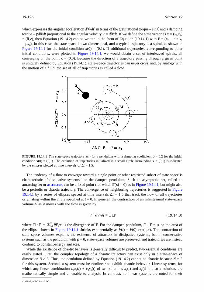
19-126 Section 19
© 1999 by CRC Press LLC
which expresses the angular acceleration d2θ/dt2 in terms of the gravitational torque – sin θ and a dampingtorque – ρdθ/dt proportional to the angular velocity ν = dθ/dt. If we define the state vector as x = (x1,x2)= (θ,ν), then Equation (19.14.2) can be written in the form of Equation (19.14.1) with F = (x2, – sin x1
– ρx2). In this case, the state space is two dimensional, and a typical trajectory is a spiral, as shown inFigure 19.14.1 for the initial condition x(0) = (0,1). If additional trajectories, corresponding to otherinitial conditions, were plotted in Figure 19.14.1, we would obtain a set of interleaved spirals, allconverging on the point x = (0,0). Because the direction of a trajectory passing through a given pointis uniquely defined by Equation (19.14.1), state–space trajectories can never cross, and, by analogy withthe motion of a fluid, the set of all of trajectories is called a flow.
The tendency of a flow to converge toward a single point or other restricted subset of state space ischaracteristic of dissipative systems like the damped pendulum. Such an asymptotic set, called anattracting set or attractor, can be a fixed point (for which F(x) = 0) as in Figure 19.14.1, but might alsobe a periodic or chaotic trajectory. The convergence of neighboring trajectories is suggested in Figure19.14.1 by a series of ellipses spaced at time intervals ∆t = 1.5 that track the flow of all trajectoriesoriginating within the circle specified at t = 0. In general, the contraction of an infinitesimal state–spacevolume V as it moves with the flow is given by
(19.14.3)
where ∇ · F = ∂Fi/xi is the divergence of F. For the damped pendulum, ∇ · F = ρ, so the area ofthe ellipse shown in Figure 19.14.1 shrinks exponentially as V(t) = V(0) exp(–ρt). The contraction ofstate–space volumes explains the existence of attractors in dissipative systems, but in conservativesystems such as the pendulum with ρ = 0, state–space volumes are preserved, and trajectories are insteadconfined to constant-energy surfaces.
While the existence of chaotic behavior is generally difficult to predict, two essential conditions areeasily stated. First, the complex topology of a chaotic trajectory can exist only in a state–space ofdimension N ≥ 3. Thus, the pendulum defined by Equation (19.14.2) cannot be chaotic because N = 2for this system. Second, a system must be nonlinear to exhibit chaotic behavior. Linear systems, forwhich any linear combination c1xa(t) + c2xb(t) of two solutions xa(t) and xb(t) is also a solution, aremathematically simple and amenable to analysis. In contrast, nonlinear systems are noted for their
FIGURE 19.14.1 The state-space trajectory x(t) for a pendulum with a damping coefficient ρ = 0.2 for the initialcondition x(0) = (0,1). The evolution of trajectories initialized in a small circle surrounding x = (0,1) is indicatedby the ellipses plotted at time intervals of ∆t = 1.5.
V V t− = ∇ ⋅1 ∂ ∂ F
Σ iN=1

Mathematics 19-127
© 1999 by CRC Press LLC
intractability. Thus, chaotic behavior is of necessity explored more frequently by numerical simulationthan mathematical analysis, a fact that helps explain why the prevalence of chaos was discovered onlyafter the advent of efficient computation.
A useful criterion for the existence of chaos can be developed from an analysis of a trajectory’s localstability. As sketched in Figure 19.14.2, the local stability of a trajectory x(t) is determined by consideringa neighboring trajectory (t) initiated by an infinitesimal deviation e(t0) from x(t) at time t0. The deviationvector e(t) = (t) – x(t) at times t1 > t0 can be expressed in terms of the Jacobian matrix
(19.14.4)
which measures the change in state variable xi at time t1 due to a change in xj at time t0. From theJacobian’s definition, we have e(t1) = J(t1,t0)e(t0). Although the local stability of x(t) is determined simplyby whether deviations grow or decay in time, the analysis is complicated by the fact that deviationvectors can also rotate, as suggested in Figure 19.14.2. Fortunately, an arbitrary deviation can be writtenin terms of the eigenvectors e(i) of the Jacobian, defined by
(19.14.5)
which are simply scaled by the eigenvalues µi(t1,t0) without rotation. Thus, the N eigenvalues of theJacobian matrix provide complete information about the growth of deviations. Anticipating that theasymptotic growth will be exponential in time, we define the Liapunov exponents,
(19.14.6)
Because any deviation can be broken into components that grow or decay asymptotically as exp(λ it),the N exponents associated with a trajectory determine its local stability.
In dissipative systems, chaos can be defined as motion on an attractor for which one or more Liapunovexponents are positive. Chaotic motion thus combines global stability with local instability in that motionis confined to the attractor, generally a bounded region of state space, but small deviations growexponentially in time. This mixture of stability and instability in chaotic motion is evident in the behaviorof an infinitesimal deviation ellipsoid similar to the finite ellipse shown in Figure 19.14.1. Because someλ i are positive, an ellipsoid centered on a chaotic trajectory will expand exponentially in some directions.On the other hand, because state-space volumes always contract in dissipative systems and the asymptoticvolume of the ellipsoid scales as exp(Λt), where Λ = λ i, the sum of the negative exponents mustbe greater in magnitude than the sum of the positive exponents. Thus, a deviation ellipsoid tracking a
FIGURE 19.14.2 A trajectory x(t) and a neighboring trajectory (t) plotted in state space from time t0 to t1. Thevectors e(t0) and e(t1) indicate the deviation of (t) from x(t) at times t0 and t1.
xx
xx
J t t x t x tij i j1 0 1 0,( ) = ( ) ( )∂ ∂
J e et t t tii
i1 0 1 0, ,( ) = ( )( ) ( )µ
λµ
i t
i t t
t t=
( )−→∞
limln ,
1
1 0
1 0
Σ iN=1

19-128 Section 19
© 1999 by CRC Press LLC
chaotic trajectory expands in some directions while contracting in others. However, because an arbitrarydeviation almost always includes a component in a direction of expansion, nearly all trajectories neigh-boring a chaotic trajectory diverge exponentially.
According to our definition of chaos, neighboring trajectories must diverge exponentially and yetremain on the attractor. How is this possible? Given that the attractor is confined to a bounded regionof state space, perpetual divergence can occur only for trajectories that differ infinitesimally. Finitedeviations grow exponentially at first but are limited by the bounds of the chaotic attractor and eventuallyshrink again. The full picture can be understood by following the evolution of a small state-space volumeselected in the neighborhood of the chaotic attractor. Initially, the volume expands in some directionsand contracts in others. When the expansion becomes too great, however, the volume begins to foldback on itself so that trajectories initially separated by the expansion are brought close together again.As time passes, this stretching and folding is repeated over and over in a process that is often likenedto kneading bread or pulling taffy.
Because all neighboring volumes approach the attractor, the stretching and folding process leads toan attracting set that is an infinitely complex filigree of interleaved surfaces. Thus, while the differentialequation that defines chaotic motion can be very simple, the resulting attractor is highly complex. Chaoticattractors fall into a class of geometric objects called fractals, which are characterized by the presenceof structure at arbitrarily small scales and by a dimension that is generally fractional. While the existenceof objects with dimensions falling between those of a point and a line, a line and a surface, or a surfaceand a volume may seem mysterious, fractional dimensions result when dimension is defined by howmuch of an object is apparent at various scales of resolution. For the dynamical systems encompassedby Equation (19.14.1), the fractal dimension D of a chaotic attractor falls in the range of 2 < D < Nwhere N is the dimension of the state space. Thus, the dimension of a chaotic attractor is large enoughthat trajectories can continually explore new territory within a bounded region of state space but smallenough that the attractor occupies no volume of the space.
Synchronous Motor
As an example of a system that exhibits chaos, we consider a simple model for a synchronous motorthat might be used in a clock. As shown in Figure 19.14.3, the motor consists of a permanent-magnetrotor subjected to a uniform oscillatory magnetic field B sin t provided by the stator. In dimensionlessnotation, its equation of motion is
(19.14.7)
where d2θ/dt2 is the angular acceleration of the rotor, –f sin t sin θ is the torque due to the interactionof the rotor’s magnetic moment with the stator field, and –ρdθ/dt is a viscous damping torque. AlthoughEquation (19.14.7) is explicitly time dependent, it can be case in the form of Equation (19.14.1) by
FIGURE 19.14.3 A synchronous motor, consisting of a permanent magnet free to rotate in a uniform magneticfield B sin t with an amplitude that varies sinusoidally in time.
d dt f t d dt2 2θ θ ρ θ= − −sin sin
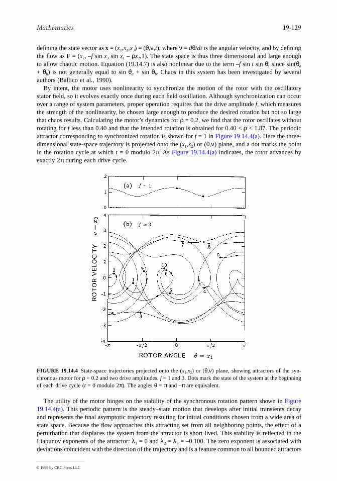
Mathematics 19-129
© 1999 by CRC Press LLC
defining the state vector as x = (x1,x2,x3) = (θ,ν,t), where ν = dθ/dt is the angular velocity, and by definingthe flow as F = (x2, –f sin x3 sin x1 – ρx2,1). The state space is thus three dimensional and large enoughto allow chaotic motion. Equation (19.14.7) is also nonlinear due to the term –f sin t sin θ, since sin(θa
+ θb) is not generally equal to sin θa + sin θb. Chaos in this system has been investigated by severalauthors (Ballico et al., 1990).
By intent, the motor uses nonlinearity to synchronize the motion of the rotor with the oscillatorystator field, so it evolves exactly once during each field oscillation. Although synchronization can occurover a range of system parameters, proper operation requires that the drive amplitude f, which measuresthe strength of the nonlinearity, be chosen large enough to produce the desired rotation but not so largethat chaos results. Calculating the motor’s dynamics for ρ = 0.2, we find that the rotor oscillates withoutrotating for f less than 0.40 and that the intended rotation is obtained for 0.40 < ρ < 1.87. The periodicattractor corresponding to synchronized rotation is shown for f = 1 in Figure 19.14.4(a). Here the three-dimensional state-space trajectory is projected onto the (x1,x2) or (θ,ν) plane, and a dot marks the pointin the rotation cycle at which t = 0 modulo 2π. As Figure 19.14.4(a) indicates, the rotor advances byexactly 2π during each drive cycle.
The utility of the motor hinges on the stability of the synchronous rotation pattern shown in Figure19.14.4(a). This periodic pattern is the steady–state motion that develops after initial transients decayand represents the final asymptotic trajectory resulting for initial conditions chosen from a wide area ofstate space. Because the flow approaches this attracting set from all neighboring points, the effect of aperturbation that displaces the system from the attractor is short lived. This stability is reflected in theLiapunov exponents of the attractor: λ1 = 0 and λ2 = λ3 = –0.100. The zero exponent is associated withdeviations coincident with the direction of the trajectory and is a feature common to all bounded attractors
FIGURE 19.14.4 State-space trajectories projected onto the (x1,x2) or (θ,ν) plane, showing attractors of the syn-chronous motor for ρ = 0.2 and two drive amplitudes, f = 1 and 3. Dots mark the state of the system at the beginningof each drive cycle (t = 0 modulo 2π). The angles θ = π and –π are equivalent.
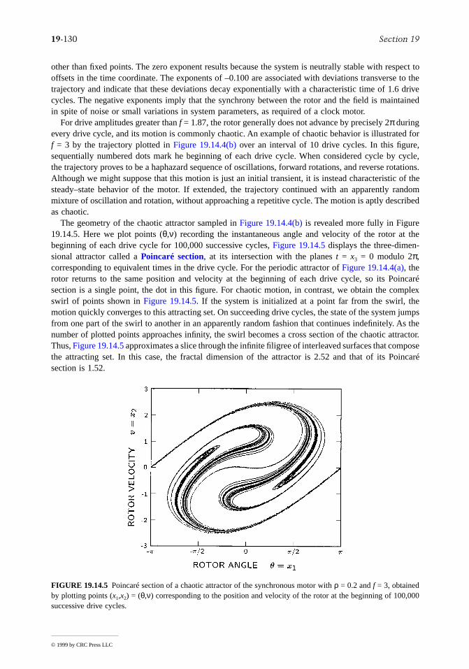
19-130 Section 19
© 1999 by CRC Press LLC
other than fixed points. The zero exponent results because the system is neutrally stable with respect tooffsets in the time coordinate. The exponents of –0.100 are associated with deviations transverse to thetrajectory and indicate that these deviations decay exponentially with a characteristic time of 1.6 drivecycles. The negative exponents imply that the synchrony between the rotor and the field is maintainedin spite of noise or small variations in system parameters, as required of a clock motor.
For drive amplitudes greater than f = 1.87, the rotor generally does not advance by precisely 2π duringevery drive cycle, and its motion is commonly chaotic. An example of chaotic behavior is illustrated forf = 3 by the trajectory plotted in Figure 19.14.4(b) over an interval of 10 drive cycles. In this figure,sequentially numbered dots mark he beginning of each drive cycle. When considered cycle by cycle,the trajectory proves to be a haphazard sequence of oscillations, forward rotations, and reverse rotations.Although we might suppose that this motion is just an initial transient, it is instead characteristic of thesteady–state behavior of the motor. If extended, the trajectory continued with an apparently randommixture of oscillation and rotation, without approaching a repetitive cycle. The motion is aptly describedas chaotic.
The geometry of the chaotic attractor sampled in Figure 19.14.4(b) is revealed more fully in Figure19.14.5. Here we plot points (θ,ν) recording the instantaneous angle and velocity of the rotor at thebeginning of each drive cycle for 100,000 successive cycles, Figure 19.14.5 displays the three-dimen-sional attractor called a Poincaré section, at its intersection with the planes t = x3 = 0 modulo 2π,corresponding to equivalent times in the drive cycle. For the periodic attractor of Figure 19.14.4(a), therotor returns to the same position and velocity at the beginning of each drive cycle, so its Poincarésection is a single point, the dot in this figure. For chaotic motion, in contrast, we obtain the complexswirl of points shown in Figure 19.14.5. If the system is initialized at a point far from the swirl, themotion quickly converges to this attracting set. On succeeding drive cycles, the state of the system jumpsfrom one part of the swirl to another in an apparently random fashion that continues indefinitely. As thenumber of plotted points approaches infinity, the swirl becomes a cross section of the chaotic attractor.Thus, Figure 19.14.5 approximates a slice through the infinite filigree of interleaved surfaces that composethe attracting set. In this case, the fractal dimension of the attractor is 2.52 and that of its Poincarésection is 1.52.
FIGURE 19.14.5 Poincaré section of a chaotic attractor of the synchronous motor with ρ = 0.2 and f = 3, obtainedby plotting points (x1,x2) = (θ,ν) corresponding to the position and velocity of the rotor at the beginning of 100,000successive drive cycles.
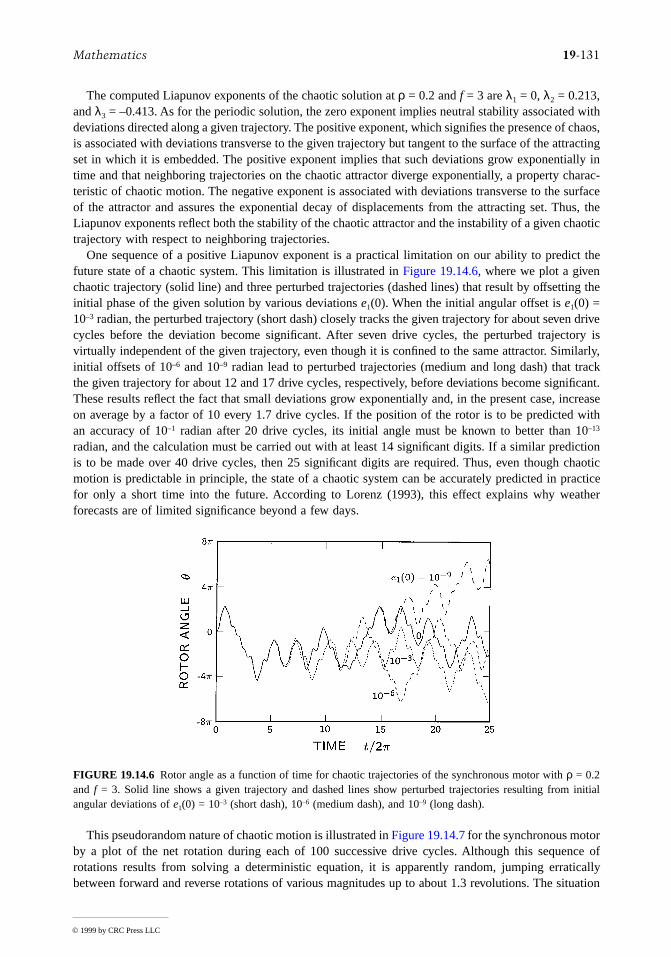
Mathematics 19-131
© 1999 by CRC Press LLC
The computed Liapunov exponents of the chaotic solution at ρ = 0.2 and f = 3 are λ1 = 0, λ2 = 0.213,and λ3 = –0.413. As for the periodic solution, the zero exponent implies neutral stability associated withdeviations directed along a given trajectory. The positive exponent, which signifies the presence of chaos,is associated with deviations transverse to the given trajectory but tangent to the surface of the attractingset in which it is embedded. The positive exponent implies that such deviations grow exponentially intime and that neighboring trajectories on the chaotic attractor diverge exponentially, a property charac-teristic of chaotic motion. The negative exponent is associated with deviations transverse to the surfaceof the attractor and assures the exponential decay of displacements from the attracting set. Thus, theLiapunov exponents reflect both the stability of the chaotic attractor and the instability of a given chaotictrajectory with respect to neighboring trajectories.
One sequence of a positive Liapunov exponent is a practical limitation on our ability to predict thefuture state of a chaotic system. This limitation is illustrated in Figure 19.14.6, where we plot a givenchaotic trajectory (solid line) and three perturbed trajectories (dashed lines) that result by offsetting theinitial phase of the given solution by various deviations e1(0). When the initial angular offset is e1(0) =10–3 radian, the perturbed trajectory (short dash) closely tracks the given trajectory for about seven drivecycles before the deviation become significant. After seven drive cycles, the perturbed trajectory isvirtually independent of the given trajectory, even though it is confined to the same attractor. Similarly,initial offsets of 10–6 and 10–9 radian lead to perturbed trajectories (medium and long dash) that trackthe given trajectory for about 12 and 17 drive cycles, respectively, before deviations become significant.These results reflect the fact that small deviations grow exponentially and, in the present case, increaseon average by a factor of 10 every 1.7 drive cycles. If the position of the rotor is to be predicted withan accuracy of 10–1 radian after 20 drive cycles, its initial angle must be known to better than 10–13
radian, and the calculation must be carried out with at least 14 significant digits. If a similar predictionis to be made over 40 drive cycles, then 25 significant digits are required. Thus, even though chaoticmotion is predictable in principle, the state of a chaotic system can be accurately predicted in practicefor only a short time into the future. According to Lorenz (1993), this effect explains why weatherforecasts are of limited significance beyond a few days.
This pseudorandom nature of chaotic motion is illustrated in Figure 19.14.7 for the synchronous motorby a plot of the net rotation during each of 100 successive drive cycles. Although this sequence ofrotations results from solving a deterministic equation, it is apparently random, jumping erraticallybetween forward and reverse rotations of various magnitudes up to about 1.3 revolutions. The situation
FIGURE 19.14.6 Rotor angle as a function of time for chaotic trajectories of the synchronous motor with ρ = 0.2and f = 3. Solid line shows a given trajectory and dashed lines show perturbed trajectories resulting from initialangular deviations of e1(0) = 10–3 (short dash), 10–6 (medium dash), and 10–9 (long dash).

19-132 Section 19
© 1999 by CRC Press LLC
is similar to that of a digital random number generator, in which a deterministic algorithm is used toproduce a sequence of pseudorandom numbers. In fact, the similarity is not coincidental since chaoticprocesses often underlie such algorithms (Li, 1978). For the synchronous motor, statistical analysisreveals almost no correlation between rotations separated by more than a few drive cycles. This statisticalindependence is a result of the motor’s positive Liapunov exponent. Because neighboring trajectoriesdiverge exponentially, a small region of the attractor can quickly expand to cover the entire attractor,and a small range of rotations on one drive cycle can lead to almost any possible rotation a few cycleslater. Thus, there is little correlation between rotations separated by a few drive cycles, and on this timescale the motor appears to select randomly between the possible rotations.
From an engineering point of view, the problem of chaotic behavior in the synchronous motor canbe solved simply by selecting a drive amplitude in the range of 0.40 < f < 1.87. Within this range, thestrength of the nonlinearity is large enough to produce synchronization but not so large as to producechaos. As this example suggests, it is important to recognize that erratic, apparently random motion canbe an intrinsic property of a dynamic system and is not necessarily a product of external noise. Searchinga real motor for a source of noise to explain the behavior shown in Figure 19.14.7 would be wastedeffort since the cause is hidden in a noise-free differential equation. Clearly, chaotic motion is a possibilitythat every engineer should understand.
Defining Terms
Attractor: A set of points in state space to which neighboring trajectories converge in the limit of largetime.
Chaos: Pseudorandom behavior observed in the steady–state dynamics of a deterministic nonlinearsystem.
Fractal: A geometric object characterized by the presence of structure at arbitrarily small scales and bya dimension that is generally fractional.
Liapunov exponent: One of N constants λ i that characterize the asymptotic exponential growth ofinfinitesimal deviations from a trajectory in an N-dimensional state space. Various componentsof a deviation grow or decay on average in proportion to exp(λ it).
Nonlinear system: A system of equations for which a linear combination of two solutions is not generallya solution.
Poincaré section: A cross section of a state-space trajectory formed by the intersection of the trajectorywith a plane defined by a specified value of one state variable.
Pseudorandom: Random according to statistical tests but derived from a deterministic process.State space: The space spanned by state vectors.
FIGURE 19.14.7 Net rotation of a synchronous motor during each of 100 successive drive cycles, illustratingchaotic motion for ρ = 0.2 and f = 3. By definition, ∆θ = θ(2πn) – θ(2π(n – 1)) on the nth drive cycle.

Mathematics 19-133
© 1999 by CRC Press LLC
State vector: A vector x whose components are the variables, generally positions and velocities, thatdefine the time evolution of a dynamical system through an equation of the form = F(x),where F is a vector function.
References
Ballico, M.J., Sawley, M.L., and Skiff, F. 1990. The bipolar motor: A simple demonstration of deter-ministic chaos. Am. J. Phys., 58, 58–61.
Holmes, P. 1990. Poincaré, celestial mechanics, dynamical-systems theory and “chaos.” Phys. Reports,193, 137–163.
Kautz, R.L. and Huggard, B.M. 1994. Chaos at the amusement park: dynamics of the Tilt-A-Whirl. Am.J. Phys., 62, 69–66.
Li, T.Y. and Yorke, J.A. 1978. Ergodic maps on [0,1] and nonlinear pseudo-random number generators.Nonlinear Anal. Theory Methods Appl., 2, 473–481.
Lorenz, E.N. 1963. Deterministic nonperiodic flow. J. Atmos. Sci., 20, 130–141.Lorenz, E.N. 1993. The Essence of Chaos, University of Washington Press, Seattle, WA.Martien, P., Pope, S.C., Scott, P.L., and Shaw, R.S. 1985. The chaotic behavior of a dripping faucet.
Phys. Lett. A., 110, 399–404.Ott, E., Grebogi, C., and Yorke, J.A. 1990. Controlling chaos. Phys. Rev. Lett., 64, 1196–1199.Singer, J., Wang, Y.Z., and Bau, H.H. 1991. Controlling a chaotic system. Phys. Rev. Lett., 66, 1123–1125.Tanabe, Y. and Kaneko, K. 1994. Behavior of falling paper. Phys. Rev. Lett., 73, 1372–1375.Wisdom, J., Peale, S.J., and Mignard, F. 1984. The chaotic rotation of Hyperion. Icarus, 58, 137–152.
For Further Information
A good introduction to deterministic chaos for undergraduates is provided by Chaotic and FractalDynamics: An Introduction for Applied Scientists and Engineers by Francis C. Moon. This bookpresents numerous examples drawn from mechanical and electrical engineering.
Chaos in Dynamical Systems by Edward Ott provides a more rigorous introduction to chaotic dynamicsat the graduate level.
Practical methods for experimental analysis and control of chaotic systems are presented in Coping withChaos: Analysis of Chaotic Data and the Exploitation of Chaotic Systems, a reprint volume editedby Edward Ott, Tim Sauer, and James A. York.
x dt•/

19-134 Section 19
© 1999 by CRC Press LLC
19.15 Fuzzy Sets and Fuzzy Logic
Dan M. Frangopol
Introduction
In the sixties, Zaheh (1965) introduced the concept of fuzzy sets. Since its inception more than 30 yearsago, the theory and methods of fuzzy sets have developed considerably. The demands for treatingsituations in engineering, social sciences, and medicine, among other applications that are complex andnot crisp have been strong driving forces behind these developments.
The concept of the fuzzy set is a generalization of the concept of the ordinary (or crisp) set. Itintroduces vagueness by eliminating the clear boundary, defined by the ordinary set theory, between fullnonmembers (i.e., grade of membership equals zero) and full members (i.e., grade of membership equalsone). According to Zaheh (1965) a fuzzy set A, defined as a collection of elements (also called objects)x ∈ X, where X denotes the universal set (also called universe of discourse) and the symbol ∈ denotesthat the element x is a member of X, is characterized by a membership (also called characteristic)function µA(x) which associates each point in X a real member in the unit interval [0,1]. The value ofµA(x) at x represents the grade of membership of x in A. Larger values of µA(x) denote higher gradesof membership of x in A. For example, a fuzzy set representing the concept of control might assign adegree of membership of 0.0 for no control, 0.1 for weak control, 0.5 for moderate control, 0.9 for strongcontrol, and 1.0 for full control. From this example, it is clear that the two-valued crisp set [i.e., nocontrol (grade of membership 0.0) and full control (grade of membership 1.0)] is a particular case ofthe general multivalued fuzzy set A in which µA(x) takes its values in the interval [0,1].
Problems in engineering could be very complex and involve various concepts of uncertainty. The useof fuzzy sets in engineering has been quite extensive during this decade. The area of fuzzy control isone of the most developed applications of fuzzy set theory in engineering (Klir and Folger, 1988). Fuzzycontrollers have been created for the control of robots, aircraft autopilots, and industrial processes, amongothers. In Japan, for example, so-called “fuzzy electric appliances,” have gained great success from bothtechnological and commercial points of view (Furuta, 1995). Efforts are underway to develop andintroduce fuzzy sets as a technical basis for solving various real-world engineering problems in whichthe underlying information is complex and imprecise. In order to achieve this, a mathematical backgroundin the theory of fuzzy sets is necessary. A brief summary of the fundamental mathematical aspects ofthe theory of fuzzy sets is presented herein.
Fundamental Notions
A fuzzy set A is represented by all its elements xi and associated grades of membership µA(xi) (Klir andFolger, 1988).
(19.15.1)
where xi is an element of the fuzzy set, µA(xi) is its grade of membership in A, and the vertical bar isemployed to link the element with their grades of membership in A. Equation (19.15.1) shows a discreteform of a fuzzy set. For a continuous fuzzy set, the membership function µA(x) is a continuous functionof x.
Figure 19.15.1 illustrates a discrete and a continuous fuzzy set. The larger membership grade max(µA(xi)) represents the height of a fuzzy set.
If at least one element of the fuzzy set has a membership grade of 1.0, the fuzzy set is called normalized.Figure 19.15.2 illustrates both a nonnormalized and a normalized fuzzy set.
The following properties of fuzzy sets, which are obvious extensions of the corresponding definitionsfor ordinary (crisp) sets, are defined herein according to Zaheh (1965) and Klir and Folger (1988).
A x x x x x xA A A n n= ( ) ( ) ( ){ }µ µ µ1 1 2 2| , | , , |K

Mathematics 19-135
© 1999 by CRC Press LLC
Two fuzzy sets A and B are equal, A = B, if and only if µA(x) = µB(x) for every element x in X (seeFigure 19.15.3).
The complement of a fuzzy set A is a fuzzy set defined as
(19.15.2)
Figure 19.15.4 shows both discrete and continuous fuzzy sets and their complements.
FIGURE 19.15.1 (a) Discrete and (b) continuous fuzzy set.
FIGURE 19.15.2 (a) Nonnormalized and (b) normalized fuzzy set.
A
µ µA Ax x( ) = − ( )1

19-136 Section 19
© 1999 by CRC Press LLC
If the membership grade of each element of the universal set X in fuzzy set B is less than or equalto its membership grade in fuzzy set A, then B is called a subset of A. This is denoted B ⊆ A. Figure19.15.5 illustrates this situation.
The union of two fuzzy sets A and B with membership functions µA(x) and µB(x) is a fuzzy set C =A ∪ B such that
(19.15.3)
FIGURE 19.15.3 Two equal fuzzy sets, A = B.
FIGURE 19.15.4 (a) Discrete fuzzy set A, (b) complement of fuzzy set A, (c) continuous fuzzy set B, and (d)complement of fuzzy set B.
AB
µ µ µC A Bx x x( ) = ( ) ( )[ ]max ,

Mathematics 19-137
© 1999 by CRC Press LLC
for all x in X.Conversely, the intersection of two fuzzy sets A and B with membership functions µA(x) and µB(x),
respectively, is a fuzzy set C = A ∩ B such that
(19.15.4)
for all x in X.Figure 19.15.6 illustrates two fuzzy sets A and B, the union set A ∪ B and the intersection set A ∩ B.
FIGURE 19.15.5 Fuzzy set A and its subset B.
FIGURE 19.15.6 (a) Two fuzzy sets, (b) union of fuzzy sets A ∪ B, and (c) intersection of fuzzy sets A ∩ B.
µ µ µC A Bx x x( ) = ( ) ( )[ ]min ,
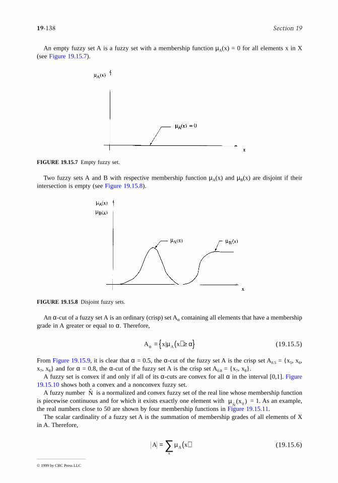
19-138 Section 19
© 1999 by CRC Press LLC
An empty fuzzy set A is a fuzzy set with a membership function µA(x) = 0 for all elements x in X(see Figure 19.15.7).
Two fuzzy sets A and B with respective membership function µA(x) and µB(x) are disjoint if theirintersection is empty (see Figure 19.15.8).
An α-cut of a fuzzy set A is an ordinary (crisp) set Aα containing all elements that have a membershipgrade in A greater or equal to α. Therefore,
(19.15.5)
From Figure 19.15.9, it is clear that α = 0.5, the α-cut of the fuzzy set A is the crisp set A0.5 = {x5, x6,x7, x8} and for α = 0.8, the α-cut of the fuzzy set A is the crisp set A0.8 = {x7, x8}.
A fuzzy set is convex if and only if all of its α-cuts are convex for all α in the interval [0,1]. Figure19.15.10 shows both a convex and a nonconvex fuzzy set.
A fuzzy number is a normalized and convex fuzzy set of the real line whose membership functionis piecewise continuous and for which it exists exactly one element with = 1. As an example,the real numbers close to 50 are shown by four membership functions in Figure 19.15.11.
The scalar cardinality of a fuzzy set A is the summation of membership grades of all elements of Xin A. Therefore,
(19.15.6)
FIGURE 19.15.7 Empty fuzzy set.
FIGURE 19.15.8 Disjoint fuzzy sets.
A x xAα µ α= ( ) ≥{ }|
Nµ ˜ ( )
Nx0
A xA
x
= ( )∑µ

Mathematics 19-139
© 1999 by CRC Press LLC
For example, the scalar cardinality of the fuzzy set A in Figure 19.15.4(a) is 2.5. Obviously, an emptyfuzzy set has a scalar cardinality equal to zero. Also, the scalar cardinality of the fuzzy complement setis equal to scalar cardinality of the original set. Therefore,
(19.15.7)
One of the basic concepts of fuzzy set theory is the extension principle. According to this principle(Dubois and Prade, 1980), given (a) a function f mapping points in the ordinary set X to points in theordinary set Y, and (b) any fuzzy set A defined on X,
FIGURE 19.15.9 α-cut of a fuzzy set.
FIGURE 19.15.10 Convex and non-convex fuzzy set.
FIGURE 19.15.11 Membership functions of fuzzy sets of real numbers close to 50.
A A=
19-140 Section 19
© 1999 by CRC Press LLC
then the fuzzy set B = f(A) is given as
(19.15.8)
If more than one element of the ordinary set X is mapped by f to the same element y in Y, then themaximum of the membership grades in the fuzzy set A is considered as the membership grade of y in f(A).
As an example, consider the fuzzy set in Figure 19.15.4(a), where x1 = –2, x2 = 2, x3 = 3, x4 = 4, andx5 = 5. Therefore, A = {0.8|–2, 0.6|2, 0.2|3, 0.4|4, 0.5|5} and f(x) = x4. By using the extension principle,we obtain
As shown by Klir and Folger (1988), degrees of association can be represented by membership gradesin a fuzzy relation. Such a relation can be considered a general case for a crisp relation.
Let P be a binary fuzzy relation between the two crisp sets X = {4, 8, 11} and Y = {4, 7} thatrepresents the relational concept “very close.” This relation can be expressed as:
or it can be represented by the two dimensional membership matrix
Fuzzy relations, especially binary relations, are important for many engineering applications.The concepts of domain, range, and the inverse of a binary fuzzy relation are clearly defined in Zadeh
(1971), and Klir and Folger (1988).The max-min composition operation for fuzzy relations is as follows (Zadeh, 1991; Klir and Folger,
1988):
(19.15.9)
for all x in X, y in Y, and z in Z, where the composition of the two binary relations P(X,Y) and Q(Y,Z)is defined as follows:
(19.15.10)
As an example, consider the two binary relations
A x x x x x xA A A n n= ( ) ( ) ( ){ }µ µ µ1 1 2 2| , | , , |K
B f A x f x x f x x f xA A A n n= ( ) = ( ) ( ) ( ) ( ) ( ) ( ){ }µ µ µ1 1 2 2| , | , , |K
f A( ) = ( ){ }= { }
max . , . | , . | , . | , . |
. | , . | , . | , . |
0 8 0 6 2 0 2 3 0 4 4 0 5 5
0 816 0 2 81 0 4 256 0 5 625
4 4 4 4
P X Y, | , , . | , , . | , , . | , , . | , , . | ,( ) = ( ) ( ) ( ) ( ) ( ) ( ){ }1 4 4 0 7 4 7 0 6 8 4 0 9 8 7 0 3 11 4 0 6 11 7
y y
x
x
x
1 2
1
2
3
1 0 0 7
0 6 0 9
0 3 0 6
. .
. .
. .
µ µ µP Q y Y P Qx z x y y zo , maxmin , , ,( ) = ( ) ( )[ ]
∈
R X Z P X Y Q Y Z, , ,( ) = ( ) ( )o
P X Y, . | , , . | , , . | , , . | , , . | , , . | ,( ) = ( ) ( ) ( ) ( ) ( ) ( ){ }1 0 4 4 0 7 4 7 0 6 8 4 0 9 8 7 0 3 11 4 0 6 11 7
Mathematics 19-141
© 1999 by CRC Press LLC
The following matrix equations illustrate the max-min composition for these binary relations
Zadeh (1971) and Klir and Folger (1988), define also an alternative form of operation on fuzzyrelations, called max-product composition. It is denoted as P(X,Y) ⊗ Q(Y,Z) and is defined by
(19.15.11)
for all x in X, y in Y, and z in Z. The matrix equation
illustrates the max product composition for the pair of binary relations P(X,Y) and Q(Y,Z) previouslyconsidered.
A crisp binary relation among the elements of a single set can be denoted by R(X,X). If this relationis reflexive, symmetric, and transistive, it is called an equivalence relation (Klir and Folger, 1988).
A fuzzy binary relation S that is reflexive
(19.15.12)
symmetric
(19.15.13)
and transitive
(19.15.14)
is called a similarity relation (Zadeh, 1971). Equations (19.15.12), (19.15.13), and (19.15.14) are validfor all x,y,z in the domain of S. A similarity relation is a generalization of the notion of equivalencerelation.
Fuzzy orderings play a very important role in decision-making in a fuzzy environment. Zadeh (1971)defines fuzzy ordering as a fuzzy relation which is transitive. Fuzzy partial ordering, fuzzy linear ordering,fuzzy preordering, and fuzzy weak ordering are also mathematically defined by Zaheh (1971) andZimmermann (1991).
The notion of fuzzy relation equation, proposed by Sanchez (1976), is an important notion with variousapplications. In the context of the max-min composition of two binary relations P(X,Y) and Q(Y,Z), thefuzzy relation equation is as follows
(19.15.15)
Q Y Z, . | , , . | , , . | , , . | , , . | , , . | , , . | , , . | ,( ) = ( ) ( ) ( ) ( ) ( ) ( ) ( ) ( ){ }0 8 4 6 0 5 4 9 0 2 4 12 0 0 4 15 0 9 7 6 0 8 7 9 0 5 7 12 0 2 7 15
1 0 0 7
0 6 0 9
0 3 0 6
0 8 0 5 0 2 0 0
0 9 0 8 0 5 0 2
0 8 0 7 0 5 0 2
0 9 0 8 0 5 0 2
0 6 0 6 0 5 0 2
. .
. .
. .
. . . .
. . . .
. . . .
. . . .
. . . .
=
o
µ µ µP Q y Y P Qx z x y y z⊗ ∈( ) = ( ) ( )[ ], max , , ,
1 0 0 7
0 6 0 9
0 3 0 6
0 8 0 5 0 2 0 0
0 9 0 8 0 5 0 2
0 8 0 7 0 5 0 2
0 9 0 8 0 5 0 2
0 6 0 6 0 5 0 2
. .
. .
. .
. . . .
. . . .
. . . .
. . . .
. . . .
×
=
µS x x,( ) = 1
µ µS Sx y y x, ,( ) = ( )
µ µ µS y S Sx z x y y z, maxmin , , ,( ) = ( ) ( )[ ]
P Q Ro =

19-142 Section 19
© 1999 by CRC Press LLC
where P and Q are matrices of membership functions µP(x,y) and µQ(y,z), respectively, and R is a matrixwhose elements are determined from Equation (19.15.9). The solution in this case in unique. However,when R and one of the matrices P, Q are given, the solution is neither guaranteed to exit nor to beunique (Klir and Folger, 1988).
Another important notion is the notion of fuzzy measure. It was introduced by Sugeno (1977). Afuzzy measure is defined by a function which assigns to each crisp subset of X a number in the unitinterval [0,1]. This member represents the ambiguity associated with our belief that the crisp subset ofX belongs to the subset A. For instance, suppose we are trying to diagnose a mechanical system witha failed component. In other terms, we are trying to assess whether this system belongs to the set ofsystems with, say, safety problems with regard to failure, serviceability problems with respect todeflections, and serviceability problems with respect to vibrations. Therefore, we might assign a lowvalue, say 0.2 to failure problems, 0.3 to deflection problems, and 0.8 to vibration problems. Thecollection of these values constitutes a fuzzy measure of the state of the system.
Other measures including plausibility, belief, probability, and possibility measures are also used fordefining the ambiguity associated with several crisp defined alternatives. For an excellent treatment ofthese measures and of the relationship among classes of fuzzy measures see Klir and Folger (1988).
Measures of fuzziness are used to indicate the degree of fuzziness of a fuzzy set (Zimmermann, 1991).One of the most used measures of fuzziness is the entropy. This measure is defined (Zimmermann, 1991)as
(19.15.16)
where h is a positive constant and S(α) is the Shannon function defined asS(α) = –α lnα – (1 – α) ln(1 – α) for rational α. For the fuzzy set in Figure 19.15.4(a), defined as
the entropy is
Therefore, for h = 1, the entropy of the fuzzy set A is 3.0399.The notion of linguistic variable, introduced by Zadeh (1973), is a fundamental notion in the devel-
opment of fuzzy logic and approximate reasoning. According to Zadeh (1973), linguistic variables are“variables whose values are not members but words or sentences in a natural or artificial language. Themotivation for the use of words or sentences rather than numbers is that linguistic characterizations are,in general, less specific than numerical ones.” The main differences between fuzzy logic and classicaltwo-valued (e.g., true or false) or multivalued (e.g., true, false, and indeterminate) logic are that (a) fuzzylogic can deal with fuzzy quantities (e.g., most, few, quite a few, many, almost all) which are in generalrepresented by fuzzy numbers (see Figure 19.15.11), fuzzy predicates (e.g., expensive, rare), and fuzzymodifiers (e.g., extremely, unlikely), and (b) the notions of truth and false are both allowed to be fuzzyusing fuzzy true/false values (e.g., very true, mostly false). As Klir and Folger (1988) stated, the ultimategoal of fuzzy logic is to provide foundations for approximate reasoning. For a general background onfuzzy logic and approximate reasoning and their applications to expert systems, the reader is referredto Zadeh (1973, 1987), Kaufmann (1975), Negoita (1985), and Zimmermann (1991), among others.
Decision making in a fuzzy environment is an area of continuous growth in engineering and otherfields such as economics and medicine. Bellman and Zadeh (1970) define this process as a “decision
d A h S xA i
i
n
( ) = ( )( )=
∑ µ1
A = −{ }0 8 2 0 6 2 0 2 3 0 4 4 0 5 5. | , . | , . | , . | , . |
d A h
h
( ) = + + + +( )
=
0 5004 0 6730 0 5004 0 6730 0 6931
3 0399
. . . . .
.

Mathematics 19-143
© 1999 by CRC Press LLC
process in which the goals and/or the constraints, but not necessarily the system under control, are fuzzyin nature.”
According to Bellman and Zadeh (1970), a fuzzy goal G associated with a given set of alternativesX = {x} is identified with a given fuzzy set G in X. For example, the goal associated with the statement“x should be in the vicinity of 50” might be represented by a fuzzy set whose membership function isequal to one of the four membership functions shown in Figure 19.15.11. Similarly, a fuzzy constraintC in X is also a fuzzy set in X, such as “x should be substantially larger than 20.”
Bellman and Zadeh (1970) define a fuzzy decision D as the confluence of goals and constraints,assuming, of course, that the goals and constraints conflict with one another. Situations in which thegoals and constraints are fuzzy sets in different spaces, multistage decision processes, stochastic systemswith implicitly defined termination time, and their associated optimal policies are also studied in Bellmanand Zadeh (1970).
References
Bellman, R.E. and Zadeh, L.A. 1970. Decision-making in a fuzzy environment. Management Science,17(4), 141–164.
Dubois, D. and Prade, H. 1980. Fuzzy Sets and Systems: Theory and Applications. Academic Press, NewYork.
Furuta, H. 1995. Fuzzy logic and its contribution to reliability analysis. In Reliability and Optimizationof Structural Systems, R. Rackwitz, G. Augusti, and A. Borri, Eds., Chapman & Hall, London,pp. 61–76.
Kaufmann, A. 1975. Introduction to the Theory of Fuzzy Subsets, Vol. 1, Academic Press, New York.Kli r, G.J. and Folger, T.A. 1988. Fuzzy Sets, Uncertainty, and Information, Prentice Hall, Englewood
Cliffs, New Jersey.Negoita, C.V. 1985. Expert Systems and Fuzzy Systems, Benjamin/Cummings, Menlo Park, California.Sanchez, E. 1976. Resolution of composite fuzzy relation equations. Information and Control, 30, 38–48.Sugeno, M. 1977. Fuzzy measures and fuzzy integrals — a survey, in Fuzzy Automata and Decision
Processes, M.M. Gupta, R.K. Ragade, and R.R. Yager, Eds., North Holland, New York, pp. 89–102.Zadeh, L.A. 1965. Fuzzy sets. Information and Control, 8, 338–353.Zadeh, L.A. 1971. Similarity relations and fuzzy orderings. Information Sciences. 3, 177–200.Zadeh, L.A. 1973. The concept of a linguistic variable and its applications to approximate reasoning.
Memorandum ERL-M 411, Berkeley, California.Zadeh, L.A. 1987. Fuzzy Sets and Applications: Selected Papers by L.A. Zadeh, R.R. Yager, S. Ovchin-
nikov, R.M. Tong, and H.T. Nguyen, Eds., John Wiley & Sons, New York.Zimmerman, H.-J. 1991. Fuzzy Set Theory – and Its Applications, 2nd ed., Kluwer Academic Publishers,
Boston.
Further Information
The more than 5000 publications that exist in the field of fuzzy sets are widely scattered in many books,journals, and conference proceedings. For newcomers, good introductions to the theory andapplications of fuzzy sets are presented in (a) Introduction to the Theory of Fuzzy Sets, VolumeI, Academic Press, New York, 1975, by Arnold Kaufmann; (b) Fuzzy Sets and Systems: Theoryand Applications, Academic Press, New York, 1980, by Didier Dubois and Henri Prade; (c) FuzzySets, Uncertainty and Information, Prentice Hall, Englewood Cliffs, NJ, 1988, by George Klirand Tina Folger, and (d) Fuzzy Set Theory and Its Applications,, 2nd ed., Kluwer AcademicPublishers, Boston, 1991, by H.-J. Zimmerman, among others.

19-144 Section 19
© 1999 by CRC Press LLC
The eighteen selected papers by Lotfi A. Zadeh grouped in Fuzzy Sets and Applications, John Wiley &Sons, New York, 1987, edited by R. Yager, S. Ovchinnikov, R.M. Tong, and H.T. Nguyen areparticularly helpful for understanding the developments of issues in fuzzy set and possibilitytheory. Also, the interview with Professor Zadeh published in this book illustrates the basicphilosophy of the founder of fuzzy set theory.

Kreith, F.; et. al. “Patent Law and Miscellaneous Topics”Mechanical Engineering HandbookEd. Frank KreithBoca Raton: CRC Press LLC, 1999
c©1999 by CRC Press LLC

20
-1
© 1999 by CRC Press LLC
Patent Law and
Miscellaneous Topics
20.1 Patents and Other Intellectual Property.........................20-2
Patents ¥ Trade Secrets ¥ Copyrights ¥ Trademarks ¥ Final Observations
20.2 Product Liability and Safety ........................................20-11
Introduction ¥ Legal Concepts ¥ Risk Assessment ¥ Engineering Analysis ¥ Human Error ¥ Warnings and Instructions
20.3 Bioengineering .............................................................20-16
Biomechanics ¥ Biomaterials
2.04 Mechanical Engineering Codes and Standards ...........20-34
What Are Codes and Standards? ¥ Codes and Standards-Related Accreditation, CertiÞcation, and Registration Programs ¥ How Do I Get Codes and Standards? ¥ What Standards Are Available?
20.5 Optics............................................................................20-40
Geometrical Optics ¥ Nonimaging Optics ¥ Lasers
20.6 Water Desalination .......................................................20-59
Introduction and Overview ¥ Distillation Processes ¥ Freeze Desalination ¥ Membrane Separation Processes
20.7 Noise Control ...............................................................20-77
Introduction ¥ Sound Propagation ¥ Human Hearing ¥ Noise Measure ¥ Response of People to Noise and Noise Criteria and Regulations ¥ Noise Control Approaches
20.8 Lighting Technology ....................................................20-85
Lamps ¥ Ballasts ¥ Lighting Fixtures ¥ Lighting EfÞciency
Frank Kreith
University of Colorado
Thomas H. Young
Dorsey & Whitney LLP
George A. Peters
Peters & Peters
Jeff R. Crandall
University of Virginia
Gregory W. Hall
University of Virginia
Walter D. Pilkey
University of Virginia
Michael Merker
American Society of Mechanical Engineers
Roland Winston
University of Chicago
Walter T. Welford (deceased)
Imperial College of London
Noam Lior
University of Pennsylvania
Malcolm J. Crocker
Auburn University
Barbara Atkinson
Lawrence Berkeley National Laboratory
Andrea Denver
Lawrence Berkeley National Laboratory
James E. McMahon
Lawrence Berkeley National Laboratory
Leslie Shown
Lawrence Berkeley National Laboratory
Robert Clear
Lawrence Berkeley National Laboratory
Craig B. Smith
Daniel, Mann, Johnson, & Mendenhall

20
-2
Section 20
© 1999 by CRC Press LLC
20.1 Patents and Other Intellectual Property
Thomas H. Young
*
The purpose of this chapter is to provide some very general information about intellectual propertyprotection (especially patents) to nonlawyers.
**
It is also intended to provide some suggestions for Òself-helpÓ to engineers that will enable them to improve the possibility of obtaining and securing appropriateprotection for their ideas and developments even before they consult a lawyer. One of the questions anintellectual property attorney frequently hears is: ÒI have a great idea. How do I protect it?Ó This sectionshould provide at least a starting point for answering that question.
In the case of patents, this section is designed to assist engineers and/or inventors in understandingwhat is expected of them and how to assist their patent lawyers or agents in the process of protectingtheir inventions. Be forewarned, however; the process of obtaining patent, trade secret, and/or copyrightprotection on such a development is not necessarily a linear one and is often neither short nor easy.
Patents
***
What is a patent?
The authorization for a patent system stems from the United Sates Constitution, whichprovides:
The Congress shall have powerÉ to promote the progress of science and useful arts, by securing forlimited times to authors and inventors the exclusive right to their resective writings and discoveries.U.S. Const. Art. I, ¤ 8.
Although the concept of a patent system did not originate in the United Sates, the drafters of theConstitution thought patents and copyrights signiÞcant enough to provide for them in the fundamentalpredicates on which our government is founded. Indeed, Thomas Jefferson, as Secretary of State, wasone of the Þrst patent Òexaminers.Ó
The premise of the Constitutional provision is to encourage the disclosure of inventions in the interestof promoting future innovation. SpeciÞcally, if inventors were not provided with patent protection fortheir innovations, they would seek to exploit them in secret. Thus, no one else would be able to beneÞtfrom and expand on their inventions, so technology would not move as rapidly as it would with fulldisclosure. Following enactment of the Constitution, Congress promptly adopted and has continuouslymaintained and updated laws implementing a patent system.
*
Mr. Young has practiced intellectual property law for more than 20 years, is a partner in the Denver ofÞceof the international law Þrm of Dorsey & Whitney, and has been an adjunct professor of patent and trademark lawat the University of Colorado law school. The author acknowledges with great appreciation the assistance of Mr.Gregory D. Leibold, an attorney focusing on intellectual property law at Dorsey & Whitney in the preparation ofthis article.
**
This section is in no way intended to provide the reader with all of the information he or she may need toevaluate or obtain intellectual property protection in particular situations on their own. Additional information isavailable from the Patent and Trademark OfÞce and the Copyright OfÞce in Washington, D.C. and other publishedreferences on these subjects. For information on patents and trademarks, the reader may contact the Commissionerof Patents and Trademarks, Washington, D.C. 20231, (703)308-3457. For information regarding copyrights, contactthe Register of Copyrights, Library of Congress, Washington, D.C. 20559, (202)707-3000. When applying the legalrequirements to a speciÞc issue, the reader is encouraged to consult with a knowledgeable lawyer.
***
The patent laws are codiÞed in 35 United States Code (i.e., ÒU.S.C.Ó) ¤ 100
et seq.
Regulations implementingthese patent laws, particularly as they relate to the operation of the Patent OfÞce, are found in volume 37 of theCode of Federal Regulations (i.e., ÒC.F.R.Ó). The internal rules of the Patent OfÞce relating to the examination ofpatents are contained in the Patent OfÞce ÒManual of Patent Examining ProcedureÓ or ÒM.P.E.P.Ó For more infor-mation on patents, the following treatises may be helpful:
Patents
, Donald S. Chisum, Matthew Bender & Co., NewYork, 1995;
Patent Law Fundamentals
, Peter D. Rosenberg, 2nd ed., Clark Boardman Callaghan, Rochester, NY,1995.

Patent Law and Miscellaneous Topics
20
-3
© 1999 by CRC Press LLC
Strictly speaking, patents are not contracts; however, because of the premise behind the Constitutionalprovision, patents have sometimes been analogized to contracts between inventors and the U.S. Gov-ernment. The Government agrees to allow the inventor exclusive rights to his or her invention for aperiod of time. In exchange, the inventor agrees to disclose his or her invention, thereby allowing otherinventors the beneÞt of the patenteeÕs work and enabling others to practice the invention after the patenthas expired.
What rights does a patent confer?
After a patent issues, the patentee has the right to exclude othersfrom making, using, or selling the subject matter claimed in the patent. Currently, the term of a U.S.patent is 20 years from the date the patent was Þled. The patentee is not required to license others touse the invention.
Nevertheless, a patent does not confer the right to do anything. In fact, it is frequently the case thatan inventor will receive a patent but will be unable to use the patented invention because it infringes onanotherÕs patent. For example, if A obtained the Þrst patent on a laser and B later obtains a patent onthe use of a laser in surgery, B cannot make or use the laser in surgery, because it would infringe AÕspatent. By the same token, however, A cannot use this laser in surgery, because it would infringe BÕspatent. In addition, patent rights are territorially limited, and the use of the same invention in differentcountries may have different ramiÞcations. Finally, regardless of patent rights, the use of certain tech-nologies (e.g., pharmaceuticals) may be limited by other government regulations and practical consid-erations.
A signiÞcant advantage of a patent over other forms of intellectual property protection, such ascopyright or trade secret, is that a patent can be enforced against anyone who utilizes the claimedtechnology regardless of whether that person copied or misappropriated the technology. Independentdevelopment of an infringing device is not a defense.
Who can obtain a patent?
Anyone who is the Þrst to invent something that falls into a category ofsubject matter that is deemed to be patentable may obtain a U.S. patent. A single patent can have severalinventors if the subject matter of one or more claims in the patent was jointly conceived or reduced topractice. In that case, each inventor, in essence, obtains his or her own rights to the patent, subject toan obligation to account to the other inventor(s) for their respective share of the remuneration. The patentmust be obtained by the true inventors or it may be invalid. Thus, persons who did not contribute to aninvention should not be named as inventors regardless of the desirability of recognizing their moral oreconomic support to the process of inventing.
What subject matter is patentable?
U.S. patent law provides that:
Whoever invents or discovers any new and useful
process, machine, manufacture, or composition ofmatter
, or nay new and useful
improvement
thereof, may obtain a patent therefore, subject to theconditions of patentability and requirements of this title. [emphasis added.] 35 U.S.C. ¤ 101.
Although the categories of patentable items seem archaic, Congress acknowledged that it intended thislanguage to Òinclude anything under the sun that is made by man.Ó
The development of signiÞcant new technologies, such as computers and biotechnology, have chal-lenged the limits of proper patentable subject matter. Nevertheless, with some diversions along the way,courts have continued to expand those boundaries so that they now include computer software andengineered life forms when embodied in properly drafted patent claims. In general, however, laws ofnature, scientiÞc truths, and mathematical algorithms are not patentable subject matter in and of them-selves. New and useful applications of those concepts, however, may be patented.
What are the standards for patentability?
In order to merit a patent, an invention must be new, useful,and nonobvious. The ÒnewÓ and ÒusefulÓ standards are deÞned precisely as one might expect. One maynot obtain a patent on an invention that has been invented before and, therefore, is not novel or on onethat has no practical utility.
The ÒnonobviousÓ standard is a more difÞcult one. Even if an invention has not been created before,in order to be patentable, it must not have been obvious to one of ordinary skill in the technical Þeld ofthe invention at the time the invention was made. In other words, a valid patent cannot be obtained on
20
-4
Section 20
© 1999 by CRC Press LLC
an invention that merely embodies a routine design or the application of principles within the ordinaryskill of the art. Whether an invention meets the standard for nonobviousness involves a factual inquiryinto the state of the art, the level of ordinary skill in the art, and the differences between what was knownin the art and the invention at the time it was made. In addition, both the Patent OfÞce and courts willlook at objective evidence of nonobviousness, including the context in which the invention was made(e.g., whether or not there was a long-standing problem that had not been solved by others), recognitionof the invention, and its success in the marketplace. Nevertheless, the determination of nonobviousnessis not precise. Indeed, the ÒbeautyÓ of many of the most signiÞcant inventions is embodied in theirsimplicity. As such, they are temptingly ÒobviousÓ after the fact, even though courts are theoreticallyconstrained from utilizing hindsight in determining nonobviousness.
How is a U.S. patent obtained?
The process of obtaining a patent starts with the invention. Invention,under U.S. patent law, has two parts. First, there is the ÒconceptionÓ of the invention, which literallyrefers to the date when the inventor Þrst thought of the novel aspect of his or her invention. Second,there is the Òreduction to practiceÓ of the invention, which can refer to a variety of activities. In the caseof a mechanical invention, for example, reduction to practice occurs when a working version of themachine is built embodying the invention. However, there is also a legal concept called ÒconstructiveÓreduction to practice, which occurs when the inventor Þles a patent application with the Patent OfÞce.
The date of invention is very important in the United States. Unlike every other country in the world,the United States awards patents to the Þrst person to invent it, rather than the Þrst person to Þle a patentapplication. Importantly, the date of conception serves as the date of invention in the United States solong as the inventor was ÒdiligentÓ in reducing the invention to practice. If the inventor is not continuouslyÒdiligentÓ (and there is some question as to what that word means, exactly), then the date of inventionis considered the date on which the inventor was continuously diligent until the invention was reducedto practice.
The date of invention can be critical to obtaining a patent in the United States. In foreign countries,however, the only date that matters is the date on which the inventor Þrst Þled the patent application.Filing a patent application in the United States will normally preserve the inventor Ôs rights abroad ifthe appropriate foreign patent applications are Þled within 1 year of the U.S. Þling date and the otherrequirements of the Patent Cooperation Treaty are met. Ideally, an inventor should Þle a patent applicationdirectly after the conception of the invention in order to achieve the earliest effective date in both theUnited States and abroad.
Before Þling a patent application, an inventor should have a Òprior art searchÓ performed.
Prior art
is a term used to refer, in part, to any printed materials published before the inventor Þles the applicationthat are relevant to the issues of novelty and nonobviousness. Having a search done for prior art is agood way to ensure that the invention for which the application is written is patentable and may alsoprovide some insight into whether or not practice of the invention would infringe the rights of others.The prior art search enables a preliminary determination of the patentability of the invention and, if itappears patentable, the identiÞcation of the patentable features to be focused upon in drafting theapplication. Nevertheless, there is always some prior art that will not be accessible using economicallyviable means at the time of application, so an inventor can never be completely sure about the noveltyof his/her invention at the time of Þling.
An inventor can apply for a patent from the Patent OfÞce either
pro se
(i.e., on his own) or througha registered patent agent or attorney. The process of obtaining a patent is a complex one, and the inventorÕschances of obtaining a valid patent of the broadest possible scope are greatly increased by the use of aqualiÞed agent or attorney. Lists of registered patent attorneys and agents are available from the PatentOfÞce. Patent attorneys may also be located through the
Martindale-Hubbell Law Directory
, state andlocal bar associations, and other publications, directories, and professional organizations.
This is not to say that inventors, themselves, have not successfully obtained patents from the PatentOfÞce. Nevertheless, busy patent examiners are easily frustrated by
pro se
applicantsÕ lack of familiaritywith patent application requirements and Patent OfÞce rules, and those frustrations are evidenced,consciously or unconsciously, in Patent OfÞce Òrejections.Ó Familiarity with the stated requirements of

Patent Law and Miscellaneous Topics
20
-5
© 1999 by CRC Press LLC
the Patent OfÞce and knowledge of its informal workings greatly increase the chances of successfullyobtaining a valid patent with the broadest possible scope.
A patent application contains a number of parts, all of which generally fall into two main categories.The Þrst group, known as the ÒspeciÞcation,Ó contains a detailed written description of the inventionincluding relevant drawings or graphs and any examples. The purpose of the speciÞcation is to ÒenableÓone of ordinary skill in the art to make and use the invention. In addition, the applicant must disclosethe Òbest modeÓ of practicing the invention. The ÒenablementÓ and Òbest modeÓ requirements are intendedto fulÞll the constitutional purpose of full disclosure of the invention. Thus, a patent that was otherwiseproperly granted by the Patent OfÞce may nevertheless be invalidated if it is later determined that theinventor failed to teach others how to utilize the invention or tried to maintain the best mode of practicingthe invention as a secret.
The second major part of the patent application is the Òclaims,Ó which are the separately numberedparagraphs appearing at the end of a patent. The claims deÞne the scope of protection that the patentwill confer, and they must be clear, deÞnite, and unambiguous. The goal of the applicant in prosecutinga patent is to obtain claims that cover the invention as broadly as possible without including subjectmatter that is obvious or not novel. For example, if A invented the two-wheeled bicycle, he might claima vehicle utilizing two round rotating objects for conveyance. Such a claim might prove to be invalid,for example, if carts were previously known. In such a situation, it would be better to claim the bicyclemore narrowly as a vehicle with two wheels in tandem.
Once the application is drafted and submitted to the Patent OfÞce, the Patent OfÞce classiÞes theinvention and sends it to an appropriate Òart unit.Ó The Patent OfÞce is divided into separate art unitsthat employ examiners who are knowledgeable about, or at least familiar with, particular Þelds oftechnology. Eventually, an examiner will read the application, focusing mainly on the claims since theydeÞne the legal parameters of the invention. After performing his own patentability search and reviewingthe application for other technical defects, the examiner may either ÒallowÓ the application to becomea patent or reject the application on the grounds that it lacks substantive merit and/or fails to complywith the formalitites of a proper patent application. If the examiner rejects some of the claims, he willexplain why the claims are not patentable in light of the speciÞc prior art references. This will start aseries of communications (in writing, by telephone, or in person) between the examiner and the applicant(or the registered attorney of record). During that process, the claims of the patent will be amended asbecomes necessary in an attempt to deÞne patentable subject matter.
If the application is eventually allowed, then the patent will be valid from the date of issuance until20 years after the date the application was originally Þled. If the application is not allowed by theexaminer and is Þnally rejected, the inventor can (1) abandon the application and the effort to obtain apatent, (2) Þle a ÒcontinuationÓ application and start the process over, or (3) appeal the rejection to theBoard of Patent Appeals and Interferences and eventually to other courts. It is not uncommon for theprocess from Þling of the application until allowance to take several years.
After the application is submitted, it is appropriate to advise the public that a patent is Òpending.ÓThis remains true until the application has been abandoned or has issued as a patent. Generally, neitherthe contents of the application nor even the fact that an application has been Þled are publicly availablefrom the Patent OfÞce absent the consent of the applicant. After the patent issues, the patent numbershould be marked on products embodying the patent. This notice serves to start the period running forthe collection of damages for patent infringement. Absent such notice, damages do not begin to run untilthe infringer receives actual notice of the patent.
Several aspects of this process bear particular note. First, once an application has been Þled, the PatentOfÞce does not permit the introduction of Ònew matterÓ into the application. Although typographicaland other simple errors in the application may be corrected, an applicant may not insert additional writtenmaterial or drawings (e.g., an additional embodiment or further improvement). The reason for this issimple Ñ because the date of invention and the date of Þling are both important for U.S. and foreignpriority purposes, the Patent OfÞce could not operate efÞciently if the subject matter of the applicationwere constantly amended. There would be numerous continuing disputes as to the effective date to be
20
-6
Section 20
© 1999 by CRC Press LLC
afforded the subject matter of an amended application. Instead, if it is necessary to amend the applicationsubstantively, a new Òcontinuation-in-partÓ application must be Þled. If it is Þled while the original orÒparentÓ application is still pending, the subject matter common to both applications will retain theoriginal Þling date, while the new material will only be afforded the Þling date of the later continuation-in-part application. The prohibition on adding Ònew matter,Ó therefore, places a premium on Þling anoriginal application that completely and accurately describes the invention.
Second, the patent application process frequently is not linear. Seldom does an invention constitutea static concept or a single Þnished embodiment. The concept may change as its full ramiÞcations areslowly revealed through practical experience, and its embodiment in physical articles, compositions, orprocesses may change after the patent application is Þled. Thus, as the invention evolves, it may benecessary to Þle further continuation-in-part applications to cover the developments which appear duringthis evolutionary process. To achieve the ultimate objective of obtaining patent protection on commer-cially viable aspects of the invention, it may be necessary for the inventor and legal counsel to reevaluatethe merits of the original application and to take appropriate corrective action in the patent prosecutionprocess.
How can the inventor help?
There are a variety of ways in which the inventor can and, in fact, shouldaid in the process of obtaining a patent.
First, and perhaps foremost, an inventor should keep detailed notes on his research and developmentthroughout the inventive process. All research and/or discoveries should be documented, dated, andwitnessed by a noninventor because they may become important later for purposes of determining whowas the Þrst to invent. The date of invention may also be useful in convincing the Patent OfÞce or acourt that certain prior art dated before the Þling of the patent application should, nevertheless, not beapplied. In preparing this documentation, it is important to realize that the testimony of the inventorhimself or documents authenticated only by the inventor are generally not sufÞcient to prove priority.There are many reasons for this. SufÞce it to say that there is a premium on having the records witnessedcontemporaneously by at least one noninventor. Getting a noninventor to witness pages of a lab notebookis one way to accomplish this. Alternatively, the Patent OfÞce will, for a nominal fee, accept and providevalidation of ÒdisclosureÓ documents evidencing the date of conception. This is probably the mostunquestionable evidence of a date of conception.
An inventor can also assist by performing an informal prior art search of his own before contactinga patent attorney. Filing a patent application is expensive. An inventor should be as conÞdent as possiblethat he has created something novel before spending the money to draft an application. Typically, apatent attorney will urge that a formal search be performed to ensure that the prior art that the PatentOfÞce examiner is likely to access has been considered. Due to the proliferation of electronic databasesfor scientiÞc and industry literature, however, there may be additional prior art which is more readilyaccessible to the inventor. A search of this material can be very helpful to the patent attorney in isolatingthe patentable features of the invention and improving the chances of obtaining a valid patent.
All prior art located by or known to the inventor should be disclosed to the patent attorney so that itcan be evaluated and disclosed to the Patent OfÞce, if necessary. In that regard, both an applicant andhis attorney are under an afÞrmative duty to disclose relevant prior art to the Patent OfÞce, and failureto do so can lead to invalidation of the patent.
Once a prior art search has been performed, an inventor should Þle an application as early as practicallypossible. As noted previously, this will protect the inventorÕs rights in foreign countries as well as provideconstructive reduction to practice of the invention if it has not already been embodied in a workingprototype. Nevertheless, some delay in Þling may be desirable in order to permit further testing andcorroboration. This is permissible, and in many instances desirable, bearing in mind that under U.S.patent law an application
must
be Þled within 1 year of the Þrst public use, disclosure, sale, or offer ofsale of the invention. This deadline cannot be extended and, if violated, will automatically result in theinvalidation of the patent. Many other countries do not have a 1 year ÒgraceÓ period; a patent applicationis immediately barred once there has been a public disclosure in that country or elsewhere. Althoughthere is an Òexperimental useÓ exception in the United States, it is limited to technical experiments (as
Patent Law and Miscellaneous Topics
20
-7
© 1999 by CRC Press LLC
opposed to test marketing) that are appropriately documented. To be safe, the inventor should contact apatent attorney before publicly disclosing or using an invention or offering it for sale. If any of thoseevents have already occurred, they should be immediately called to the patent attorneyÕs attention.
The inventor is also instrumental in drafting the patent application. The inventor must make sure thatthe speciÞcation is accurate, enables one skilled in the art to practice the invention, and discloses thebest way to make and use the invention. Although the art of claim drafting is somewhat of an acquiredskill, the inventor should also be very involved in that process to make sure that the claims cover theinvention and are not easily designed around. Sometimes a patent attorney will draft claims that do notexpressly state a physical element or process step, but utilize Òmeans-plus-functionÓ language. In thatcase, it is highly desirable to describe as many means as possible for fulÞlling that element in theapplication itself, and the inventor is the best source of that type of information. In other words, theinventor should continuously be asking questions of his attorney about whether or not certain variationsof his invention will be adequately protected by the claims as drafted. Finally, the inventor can andshould be instrumental in helping the attorney identify the technical/practical differences between theinvention and prior art. In short, the prosecution of a patent application should be a team effort betweeninventor and attorney at each step in the process.
Trade Secrets
*
In some instances it may be desirable to protect new technology as a trade secret rather than by patent.For example, an invention may not be patentable; it may be one of numerous small items or ÒknowhowÓ that improve oneÕs business. Such items are typically protected as trade secrets. While there is noformal method of acquiring trade secret protection as there is for patents and copyrights, attention muststill be paid to their identiÞcation and protection. Also, unlike patents and copyrights, trade secrets areprotected under state, rather than federal laws. Therefore, the nuances of trade secret protection mayvary depending on which stateÕs laws apply. There are, however, some general principles of trade secretsthat are common to most jurisdictions.
What is a trade secret?
A Òtrade secretÓ may include anything that gives a person an advantage overhis competitors and is not generally known to them. It includes compilations of information such ascustomer lists, compositions, process techniques and parameters, and software. In determining whetheror not something is a protectable trade secret, courts look at the following factors: (1) the extent to whichthe information is known outside of the trade secret ownerÕs business; (2) the extent to which it is knownby employees or others involved in the trade secret ownerÕs business; (3) the extent of measures takenby the trade secret owner to guard the secrecyof the information; (4) the value of the information to thetrade secret owner and to his competitors; (5) the amount of effort or money expended by the tradesecret owner in developing the information; and (6) the ease or difÞculty with which the informationcould be properly acquired or duplicated by others.
What protection does a trade secret provide?
A trade secret protects the owner from improperappropriation of the secret through use or disclosure by a person having an obligation not to do so. Themajor advantage of a trade secret is that it may last indeÞnitely; the major defect is that if it is lost, itgenerally cannot be reclaimed. Unlike patent infringement, a person accused of stealing a trade secretcan successfully defend such an accusation by showing that he independently developed the subjectmatter of the secret. Trade secret protection, therefore, is only as good as the inability of competitorsto Òreverse engineerÓ or independently develop it.
How can one obtain a trade secret?
Whether or not one has a trade secret is ultimately determinedjudicially in an action for enforcement. The court will look at all of the factors previously noted. At thattime it is usually too late to take the actions necessary to establish trade secret protection. Thus, thereis a premium for the periodic review and implementation of a program for trade secret protection. Among
*
See, generally, the Uniform Trade Secrets Act ¤ 1(4), 14 U.L.A. 537 (1980) and
Milgrim on Trade Secrets
,Roger M. Milgrim, Matthew Bender & Co., New York, 1995.

20
-8
Section 20
© 1999 by CRC Press LLC
the steps that can be taken to protect trade secrets are (1) identifying the types of materials that aredeemed to be trade secrets by an organization and notifying employees of the organizationÕs policy totreat this information as trade secrets; (2) restricting access to the trade secrets to only those individualswho have a need to know and who are obligated by contract or otherwise not to use or disclose them;(3) taking physical precautions to limit access to trade secrets such as using locked Þle cabinets, vaults,etc. These are the most fundamental steps that can be taken.
Although legal counsel is frequently consulted in establishing a plan for protecting trade secrets,including the drafting of appropriate conÞdentiality agreements, the physical steps required should beput in place by the trade secret owner prior to legal consultation.
Copyrights
*
Copyright protection is usually associated with writings, songs, paintings, sculpture, and other artisticendeavors. However, it also extends to certain technology, particularly software, databases, and certainarchitectural plans.
What protection does a copyright provide?
Copyright protection is a matter of federal law. Under thefederal Copyright Act, protection is available for ÒoriginalÓ works of appropriate subject matter, suchas those mentioned in the previous paragraph. A copyright provides the exclusive right to reproduce,publicly distribute, publicly perform, publicly display, and make derivative works from an original workof authorship. However, it protects only against ÒcopyingÓ of the protected work and does not provideprotection where a work has been independently developed by another. Copying can be presumed wherethe third party had access to the copyrighted work and there is Òsubstantial similarityÓ between the thirdpartyÕs work and the original. Further, in certain limited instances, a small portion of a work may bereproduced without liability as a Òfair use.Ó The parameters of the Òfair useÓ doctrine are complicated,however, and they are beyond the subject of this section.
Only a modicum of creativity is needed to satisfy the requirement of Òoriginality.Ó On the other hand,protection is limited. It has frequently been stated that a copyright only protects the manner in whichsomething is expressed, rather than the idea or content, which can be an extremely difÞcult distinctionto make. For example, there is signiÞcant debate as to the appropriate scope of copyright protection, forboth software and databases. Nevertheless, an advantage of a copyright is that it may last for a relativelylong period of time. At a minimum, copyright in works created at this time last for the life of the authorplus 50 years.
How is a copyright obtained?
Theoretically, in order to obtain a copyright an author need only showthat a work is original to him (i.e., that he is in fact the author). Federal protection for copyright attachesas soon as a writing is Þxed in a tangible medium (i.e., as soon as it is put on paper, or in memory ona computer, or anywhere else that it can be ÒperceivedÓ). Nevertheless, there are two important stepsthat should be taken to realize the full scope of that protection.
First, it is highly advisable to afÞx a copyright notice to the work. ÒNoticeÓ is provided by afÞxingto the work: (1) the word ÒCopyrightÓ or the Ò©Ó symbol, (2) the date of Þrst publication, and (3) thename of the copyright owner. Notice should be afÞxed to the work in an obvious position (such as oneof the Þrst pages of a book, an entry screen of a computer program, etc.). A copyright notice should beplaced on all drafts of material that may be subject to protection under copyright law. If an author failsto put the notice on his work, copyright protection is not lost; however, an infringer may then use thedefense that he innocently thought that the work was within the public domain. Adequate notice precludesthe ÒinnocentÓ infringer defense, and, because it does not cost anything, notice is always a good idea.
In addition, registration of the copyright with the Register of Copyrights at the Library of Congressis also highly recommended. This procedure is relatively simple and inexpensive. It consists of Þlling
*
The federal laws on copyright are codiÞed in the Lanham Act, ¤ 1
et seg.
For further information on copyrights,the following treatise may be helpful:
Nimmer on Copyright
, Melville B. & David Nimmer, Matthew Bender & Co.,New York, 1995.
Patent Law and Miscellaneous Topics
20
-9
© 1999 by CRC Press LLC
out a government form and submitting it with the appropriate Þling fee and a sample of the work soughtto be copyrighted. If the application is acceptable, the Copyright OfÞce returns a copy of the applicationstamped with the copyright registration number.
In the case of software and databases, there has been concern that an unscrupulous competitor mightattempt to purloin valuable information from the sample submitted with the application. In recognitionof this problem, the Copyright OfÞce has promulgated rules allowing the submission of only a limitedportion of the software or database adequate to identify the copyrighted work.
Although federal registration is not necessary to perfect a copyright, it does have some signiÞcantadvantages. First, it is necessary to obtain a registration in order to bring suit against an infringer. Whileit is possible to register the work on an expedited basis immediately prior to commencing the lawsuit,it is not advisable. Early registration (i.e., within 3 months of the Þrst publication of the work) allowsan author to elect to sue for ÒstatutoryÓ damages, which can be considerably easier to prove and, possibly,more muniÞcent than ÒactualÓ damages. In addition, an author may be able to recover attorneysÕ feesfrom a defendant in some cases, but only if the work in question was registered before or soon afterpublication. In sum, if an author believes that a work is important and might be copied, he shouldpromptly register the work.
Trademarks
*
Although trademark protection does not encompass technology per se, any summary of intellectualproperty protection would be incomplete without a few comments on the scope and availability oftrademark rights.
What is a trademark?
A trademark is anything that serves to identify the source of a product orservice. Trademark protection can be obtained on a wide variety of items such as words, symbols, logos,slogans, shapes (if they are not functional), tones (such as NBCÕs three-note tone), and even colors. Atrademark owner may assert his rights against a third party that is engaged in conduct that is likely tocause consumers to believe that his goods or services emanate from, are associated or afÞliated with,or are sponsored by the trademark owner.
The purpose of trademark protection is twofold: (1) to ensure the public that goods or services offeredunder a trademark have the quality associated with the trademark owner and (2) to preserve the valuablegoodwill that the trademark owner has established by promoting the mark. Trademark rights may lastindeÞnitely.
How are trademark rights established?
Trademarks are protected under both federal and state law.There are two ways to obtain rights in a trademark: use or federal registration. Rights in a mark can beacquired simply by using the mark in connection with the goods and services. If the mark is a distinctiveone (i.e., coined or Òmade-upÓ like ÒPOLAROIDÓ) rights are established immediately. On the otherhand, if the mark is descriptive, the use must be so prominent and lengthy that the mark has acquireda Òsecondary meaning,Ó (i.e., the public has come to recognize the term as identifying the source of thegoods and services rather than as a reference to the product or service itself). In either case, to establishrights through use, it is desirable to use the designation Ò
ª
Ó in connection with the mark, therebyindicating that the owner of the mark asserts that it is a trademark under common law.
In contrast, the process of obtaining a federal trademark registration involves the Þling of an applicationwith the U.S. Patent and Trademark OfÞce. The application identiÞes the mark, the goods and serviceswith which it is used, and, if it is already in use, the date of Þrst use and the date of Þrst use in interstatecommerce. A Þling fee is also required but is relatively minimal. A trademark examiner will check theapplication substantively, including the review of previously issued trademarks, to see if there is anyconßict. If the examiner allows the application, the mark is published in the
OfÞcial Gazette
, which is
*
The federal trademark laws are codiÞed at 17 U.S.C. ¤ 1
et seg.
For further information on trademarks, thefollowing treatise may be helpful:
McCarthy on Trademarks and Unfair Competition
, J. Thomas McCarthy, ClarkBoardman Callaghan, Rochester, NY, 3rd ed., 1995.
20
-10
Section 20
© 1999 by CRC Press LLC
a weekly publication of the Patent OfÞce. If no one opposes the registration within 30 days afterpublication, then a registration will be issued. If there is an objection, then an opposition proceeding isinitiated, and the applicant and the opposer essentially litigate to determine who should obtain thetrademark registration. Provided that certain documents are subsequently Þled with the Patent OfÞce toafÞrm and renew the registration, the registration may last indeÞnitely. The existence of a federallyregistered trademark is designated by the symbol Ò
¨
Ó, which is frequently seen on the shoulder of themark.
A federal trademark registration is a powerful tool in protecting a trademark. By law it serves asÒconstructiveÓ (i.e., assumed) notice of the registrantÕs claim of rights throughout the United States. Inessence, the registration acts like a recorded deed to real estate, and anyone who subsequently purchasesthat property without checking the recorded information does so subject to the interests of record. Incontrast, the rights of one who attempts to acquire a trademark only through use are generally limitedto the geographic area in which the mark is actually used. Others who subsequently use the mark inother areas of the country may also establish rights. Thus, the Þrst step in selecting a trademark is tosearch the records of the Patent OfÞce to determine whether or not a confusingly similar mark haspreviously been registered. Typically, a trademark search performed by a professional search organizationwill also reveal state registrations and other common law uses that might cause conßicts with the markunder consideration.
One other advantage to federal registration is that the registrant may begin to acquire protection ona mark prior to actual use. This is accomplished by Þling an Òintent-to-useÓ application on a mark thatthe applicant has made a
bona Þde
decision to use. The application is examined as described previously.Although the mark must actually be placed in use before the registration is issued, the registration willbe effective from the date of its Þling. Thus, the public is on notice of the applicantÕs potential rightsas soon as the application is Þled. The examination process will also give the applicant signiÞcant comfortthat the mark is available for use before investing a great deal of money in its promotion.
Final Observations
Selecting an appropriate method of acquiring intellectual property protection for a new developmentmay involve several forms of protection. Software, for example, may be protected by patent, trade secret,and copyright protection and may be sold using a registered trademark. In addition, other legal meansmay be used to protect the software, including appropriate contractual provisions limiting and restrictingthe rights of a user acquired by license. Those contractual commitments may survive, even if theintellectual property protection is lost.
It is hoped that this section has provided at least a general overview by which the nonlawyer canbegin to understand how to protect intellectual property. There are almost never any easy answers to thequestion of how to protect products, ideas, and services, and it is always advisable to consult a qualiÞedattorney with speciÞc questions. A knowledgeable client, however, can make a signiÞcant difference inachieving the strongest protection available.

Patent Law and Miscellaneous Topics
20
-11
© 1999 by CRC Press LLC
20.2 Product Liability and Safety
George A. Peters
Introduction
Almost all engineers, at some time in their career, can expect some direct contact or indirect involvementwith the legal system. The contact may be in the form of having to answer written interrogatories ontechnical issues for a company defendant or plaintiff, being personally deposed and having to respondto oral questions under oath, appearing for a company during trial, assisting lawyers in a lawsuit, orpersonally being a defendant in a lawsuit. Most important is having the ability to translate legalrequirements into engineering speciÞcations to assure compliance with the law.
The old maxim Òignorance of the law is no excuseÓ should be supplemented by an understanding thatignorance of the law may result in unnecessary mistakes (illegal acts) and personal fear when Þrstconfronted by an unknown aspect of the legal process. It is essential that the engineer have sufÞcientunderstanding to avoid gross errors and omissions, to react appropriately to legal proceedings, and towant to build a basic foundation of knowledge that can be quickly enhanced when needed. This sectionis only a brief overview that might be illustrative and helpful in both understanding potential legalliability and how to avoid, prevent, or proactively minimize any such legal exposure. If product liabilityis legal fault for an unsafe design, the question then becomes how to achieve an appropriate level of safety.
Legal Concepts
Fundamental to determining who might be legally Òat faultÓ is the concept of
negligence
which is utilizedworldwide in the apportionment of damages (legal redress). Negligence is the failure to exercise ordinaryor reasonable care, which persons of ordinary prudence would use to avoid injury to themselves orothers. The exact deÞnition is given to jurors, usually in the form of approved jury instructions (theactual operative law), who then apply the law given to them to the facts and circumstances of the casebefore them. The defenses to allegations of negligence (absence of due care) are, usually,
contributorynegligence
(fault) on the part of the plaintiff or
assumption of the risk
on the part of the plaintiff (thatrisk that is speciÞc and voluntarily assumed, not general or coerced). If there is a violation of a statuteor regulation there may be a rebuttable presumption of negligence. Compliance with a technical standardmay be some evidence of the exercise of due care. Concepts of
strict liability
involve the presence of adefect that legally caused personal injury or property damage. There are many deÞnitions of a
defect
,such as a failure to perform as safely as an ordinary consumer would expect when used in an intendedor reasonably foreseeable manner or Òexcessive preventable risks.Ó
Foreseeability
means that the personal injury, property damage, or environmental harm must havebeen predictable or knowable at the time of design, manufacture, or sale of the product. Generally, thelaw requires only
reasonable efforts
to prevent defects, deÞciencies, or unsafe conditions. In other words,there should be efforts to predict possible harm and reasonably practical risk reduction efforts to minimizethe harm.
The term
engineering malpractice
includes conduct that has personal legal consequences (professionalliability) for the individual engineer, conduct that has adverse legal consequences for his or her employer(such as product liability or toxic torts), and conduct having moral or ethical consequences even thoughit may be legally protected (Peters, 1996a).
There are many other supplemental legal concepts and each state or jurisdiction has summaries ofthe law (Witkin, 1987Ð1990), approved jury instructions (Breckinridge, 1994), statutes enacted by thelegislature, compendiums of case law decisions by the courts, and regulations issued by executiveagencies (all of which are constantly being revised and expanded). Thus, the engineer should alwaysconsult with an attorney-at-law before making an interpretation or taking any action that might be withinthe province of a licensed professional.

20
-12
Section 20
© 1999 by CRC Press LLC
There are thousands of technical standards issued by professional associations, trade groups, standardsformulation organizations, and government agencies. Compliance with such standards is the Þrst line ofliability prevention, but such standards should be exceeded by a confortable margin to accommodatedesign, material, fabrication, and in-use process variance (Council, 1989). However, there are otherimportant liability prevention measures that should be undertaken during the design process and describedin a product liability prevention plan.
Risk Assessment
A central theme in liability prevention is Òrisk assessmentÓ. The Þrst step in such an assessment is toidentify all probable
hazards
(those faults, failures, or conditions that could cause harm), then determinethe quantitative
risk
for each (the frequency and severity of harm), and, Þnally, render a subjectivejudgment as to
danger
(the presence of excessive preventable danger). It is important to determine whatkind of risk assessment is being made and to identify its objective as follows:
1.
Compliance
. The exact method of conducting a risk assessment may be speciÞed by procurementspeciÞcations, industry standards, or government regulations. The design objective may be onlycompliance with the assessment requirement. However, in the process of performing a writtenrisk assessment and classifying the risk into some severity level, it may result in a beneÞcialsafety audit of the product. Where there is Òresidual risk,Ó the design of speciÞc warnings andinstructions may be required.
2. Major Compliance Tasks. Where safe performance is very important, a detailed engineeringanalysis may be required by contract or regulation. This might involve listing all probable hazardsfor each component, part, and subsystem, then attempting to quantify the risk estimate for eachhazard at the 10Ð6 level of attempted precision. Since this requires a major effort, the primarydesign and management objective should be product improvements and informed product assur-ance.
3. Comparative Analysis. Some risk assessments involve only an overall risk estimate which is thencompared with other similar products or a wide range of products. The objective or use may befor marketing purposes or liability defense. Since the results are gross or macroscopic, such riskassessments generally do not result in product improvement.
4. Risk Ratings. Some trade associations may provide generic risk ratings for materials or products.The objective may be for an Òinformed choiceÓ of procedures and Þeld equipment in order tosatisfy a legal Òduty of careÓ or to help determine the Òbest practical meansÓ of job performance.
5. System Effectiveness. Some risk assessments are performed early in the design process, perhapsas part of a reliability analysis, for the purpose of predicting Þnal system effectiveness. Theobjective may be to check design efforts, reallocate available funds, or refocus management auditsto achieve a desired level of system effectiveness. The process may be used to assure that desiredsystem-of-systems performance is achievable.
From the societal viewpoint, some level of risk can be tolerable, acceptable, required, and speciÞed.What is desired at a given locality or time period can be made known by the local common law,government regulations, trade standards, practices, customs, and expectations. From the engineeringviewpoint, risk levels are controllable, adjustable, manageable, and a consequence of the applicationof appropriate engineering techniques, skills, and information resources.
Engineering Analysis
Rather than rely only upon an engineerÕs subjective and often biased judgment as to what constitutes asafe design, it is advisable to perform speciÞc objective engineering analyses for design safety. Thisusually includes some systematic approach to identifying failure modes and Þeld hazards, their riskconsequences, and alternative design options that might improve the safety performance. This should

Patent Law and Miscellaneous Topics 20-13
© 1999 by CRC Press LLC
be supplemented by formal design review sessions that consider information from or about customersand learned intermediaries in the fabrication, packaging, shipping, distribution, and marketing system.Written hazard analyses should include consideration of legal duties (Peters, 1991a,b), liability preventiontechniques (Peters, 1996b), and cultural attributes and technical information resources in the worldwidemarketplace (Murakami, 1987, 1992). There should be a systems perspective, a cradle-to-ultimate-disposal philosophy, a true understanding of customer needs and characteristics, and appropriate appli-cation of speciÞc design safety techniques.
Testing is required to verify the engineering analyses, to prove the inherent safety of the product orprocess system, and to discover all potential problems before they become manifest postsale. As part ofa product liability mitigation plan, procedures and costs should be determined for possible accidentinvestigations, product recalls, retroÞts, and injury reparations. A continuing (postsale) product surveil-lance plan should cover all foreseeable users, servicing, maintenance, repair, modiÞcation, transport,disposal, and recycling of the product and its components. This permits early discovery and resolutionof safety problems. It should also include a means for updating a knowledge bank of scientiÞc, engi-neering, legal, insurance, patent, and foreign standards information useful for future design efforts aswell as postsale obligations.
Human Error
Human error is a major source of undesirable variance in humanÐmachine interfaces. Unfortunately,many engineers neglect or virtually ignore the human factors aspects of product and system design.There should be some effort to control human performance and prevent human failure by designing fora wide range of human dimensions, characteristics, and predictable responses (Peters, 1996a). If possible,the physical attributes, kinetics, and creative perceptual abilities of human operators, maintenance andrepair personnel, and bystanders should be utilized in design. Human factors should be part of any earlyengineering analysis, with appropriate testing and safeguarding for human error that cannot otherwisebe eliminated. This includes mechanical guards, tamper-resistant features, safe-stop and limited move-ment switches, proximity sensors with directional control, built-in time for protective behavioral reac-tions, and the prevention of inadvertent activation and operation. One of the most important sources ofhelpful information on human error comes from incident and accident reconstruction, but the scope andbias of the inquiry may severely limit the design usefulness of the data obtained; for example,
1. The fatalistic approach where human error is considered as being inevitable in an imperfectworld. If there is Òno faultÓ other than by the person committing an error or omission, there islittle incentive to investigate in detail to determine other factors for purposes of corrective action.This fosters the continuance of tolerable human error, persistent undesirable human error, and alack of true recognition of causation and preventive actions.
2. The behavioral approach which has a focus on individual behavior in an attempt to develop Òsaferpeople,Ó safer attitudes, and to develop motivation to Òact responsibly.Ó This may result in closersupervision and additional training, with some short-term beneÞts, but it does not permanentlyalter the error-inducing situation.
3. The situational approach to human error is to blame the situation, the work environment, groupinteractions, sociotechnical factors, and the overall circumstances of the situation. There is somebeneÞt from a broader perspective to human error since it provides a better understanding ofcausation.
4. The product design approach has an emphasis on the interaction between the user and theengineered product to provide information useful to the design engineer.
5. The multifactorial approach is based on the assumption that there is multiple causation for eachinjury, damage, loss, harm, or error. If special attention is given to each substantial factor or cause,valuable design-oriented information can result. This multifaceted perspective of accident recon-struction has the greatest beneÞt and is compatible with concepts of pure comparative negligenceand the allocation of damages in proportion to the degree of fault.
20-14 Section 20
© 1999 by CRC Press LLC
During any accident investigation or accident reconstruction, care should be exercised to prevent anyÒspoliationÓ or distruction of evidence. This requires trained specialists, since even slight changes to theproduct may obliterate information that becomes critical in later product evaluations.
Warnings and Instructions
As a last resort, for residual risk, appropriate use of warnings and instructions is essential for productliability prevention and the safe use of products (Peters, 1993). Such communications require a speciÞcdesign engineering effort, plus relevant testing, if they are to be effective. They include warning devices,warnings on labels and packaging, material safety data sheets, instructions for training, insertions inowner's or operator's manuals, and postsale advertisements and letters to all owners. Some regulationsrequire that they be in two languages and in nonlanguage pictorials. Such hazard communications andprocedural directions should not be the result of a cursory afterthought, but an ongoing integral part ofthe design process. There may be neuropsychological considerations in the presentation of informationby visual or auditory displays, machine condition and status indicators, and computer-generated infor-mation that requires specialized knowledge and testing. The basic premise is to design a referent abouta speciÞc hazard so the target individual is adequately informed as to risk and has a reasonable choiceas to avoidance behavior. Warnings that fail to communicate their intended message are functionallyuseless. There is considerable scientiÞc and engineering information regarding the design of warningsand instructions, and the failure to heed such information may result in legal allegations about a failureto warn, instruct, test, or appropriately market a product. The issue becomes what proof exists aboutwhether or not warnings, instructions, or representations would have signiÞcantly inßuenced user behav-ior, purchaser choices (as, for example, in available options), and use of protective equipment. Warningsare an important liability prevention and design safety objective.
References
Breckenridge, P.G., Ed. 1994. California Jury Instructions. 2 vols., West Publishing, St. Paul, MN.Council Directive of 14 June 1989 on the approximation of the laws of the Member States relating to
machinery (89/392/EEC), as amended 20 June 1991 (91/368/EEC) and 14 June 1993 (93/44/EEC).Note: the Council is the Council of the European Communities. Conformity is indicated by theCE mark on machinery and safety components which must be accompanied by an EC declarationof conformity (93/465/EEC).
Murakami, Y., Ed. 1987, 1992. Stress Intensity Factors Handbook, Vols. 1 and 2 (1987), Vol. 3 (1992),The Society of Material Science (Japan), and Pergamon Press, Elmsford, NY.
Peters, G.A. 1991a. The globalization of product liability law, Prod. Liability Law J., Butterworth LegalPublishers, 2(3), 133Ð145.
Peters, G.A. 1991b. Legal duty and presumptions that are compatible with current technology and futureworld trade, Prod. Liability Law J., Butterworth Legal Publishers, 2(4), 217Ð222.
Peters, G.A. 1993. Warnings and alarms, Chap. 4 in Vol. 5 of Automotive Engineering and Litigation,Peters, G.A. and Peters B.J., Eds., John Wiley & Sons, New York, 93Ð120.
Peters, G.A. 1996a. Engineering malpractice and remedies: advanced techniques in engineering liability,Technol. Law Insurance, 1, 3Ð9.
Peters, G.A. 1996a. Human error prevention, Chap. 8 in Asbestos Health Risks, Vol. 12 of the Sourcebookon Asbestos Diseases, G.A. Peters and B.J. Peters, Eds., Michie, Charlottesville, VA, 207Ð234.
Peters, G.A. 1996b. Liability prevention techniques, in Proceedings of the JSME International Sympo-sium on Product Liability and Failure Prevention, Fukuoka, Japan, 167Ð184.
Witkin, B.E. 1987Ð1990. Summary of California Law, 9th ed., 13 vols., Bancroft-Whitney, San Francisco.

Patent Law and Miscellaneous Topics 20-15
© 1999 by CRC Press LLC
Further Information
For more detailed information, on product liability and safety, readPeters, G.A. and Peters B.J., Eds. Sourcebook on Asbestos Diseases: Medical, Legal, and Engineering
Aspects, 14 vols. Michie, Charlottesville, VA, 1980Ð1997.Peters, G.A. and Peters B.J., Eds. Automotive Engineering and Litigation, 6 vols. John Wiley & Sons,
New York, 1984Ð1993.

20-16 Section 20
© 1999 by CRC Press LLC
20.3 Bioengineering
Jeff R. Crandall, Gregory W. Hall, and Walter D. Pilkey
The interdisciplinary Þeld of bioengineering combines personnel and principles from the physical andlife sciences. Although a relatively young Þeld, it is developing rapidly by incorporating experimentaland computational techniques from traditional disciplines of engineering and applying them to biologicalproblems. In particular, Þnite-element techniques and computer modeling are revolutionizing the mannerin which bioengineering is conducted and interpreted.
Although based on the principles of traditional disciplines, bioengineering differs from classicalengineering because the human body is a living system capable of responding to a changing environment.This results in several challenges for the bioengineer:
¥ Material properties can vary due to intrinsic and extrinsic factors, e.g., physical properties changewith specimen age, gender, and health;
¥ The human body is capable of self-repair and adaptation, e.g., muscle size increases in responseto physical training;
¥ Many structures within the body cannot be isolated for laboratory testing, e.g., the heart cannotbe removed to study circulatory system mechanics.
The discipline of bioengineering includes, but is not limited to, the topics of
¥ Biomechanics
¥ Biomaterials
¥ Biomedical instrumentation and sensors
¥ Biotechnology
¥ Genetic engineering
¥ Medical imaging
¥ Clinical engineering.
Due to the vast breadth of the Þeld, the authors of this section have not attempted to provide an exhaustiveoverview of the Þeld of bioengineering but rather have tried to select those areas believed to be of mostinterest to mechanical engineers. Therefore, this summary of bioengineering is intended to acquaint thereader with the concepts and terminology within the Þelds of biomechanics and biomaterials and toprovide basic material properties for both tissues and implanted devices.
Biomechanics
The Þeld of biomechanics applies the theories and methods of classical mechanics to biological systems.More precisely, it is concerned with the forces that act on and within a biological structure and with theeffects that these forces produce. An overview of topics within the Þeld of biomechanics is provided inFigure 20.3.1. It is evident that the study of stress and strain distributions in biological materials for thedevelopment of constitutive equations is a major research emphasis. A review of the constitutive equationsand the associated material properties are provided in this section for the most commonly tested tissues.
Hard Tissue Mechanics
The term bone refers to two types of hard tissue structure: cortical and cancellous bone. Cortical boneis the dense, structured compact bone that composes the shaft of long bones such as the femur and tibia.Cancellous or trabecular bone is found within the ends of tubular bones and the body of irregularlyshaped bones. The mechanical and structural properties of the two types of bone can vary substantially.In addition, bone is capable of remodeling in response to its environment. Table 20.3.1 summarizes thegeneral physical and material properties for the two bone types.

Patent Law and Miscellaneous Topics 20-17
© 1999 by CRC Press LLC
Like most biological materials, bone behaves as an anisotropic, nonhomogeneous, viscoelastic mate-rial. Therefore, the values in Table 20.3.1 exhibit a wide range of scatter and variability due to thesimpliÞed model of bone as a linearly elastic isotropic material. It is generally adequate, however, tomodel bone as a linearly elastic anisotropic material at the strain rates found in most experiments. Toaddress the anisotropy of bone, bone is generally considered to exhibit either transverse isotropic ororthotropic behavior. The constitutive equation for a linearly elastic material can be written using asingle-index notation for stress and strain as
(20.3.1)
where the standard summation convention is used with the indexes possessing a range of 6. The stress-strain relationship can be similarly expressed in terms of the compliance matrix sij such that
(20.3.2)
Equation (20.3.3) represents the compliance matrix of an orthotropic material in terms of the YoungÕsmoduli (Ei), the PoissonÕs ratio (nij), and the shear moduli (Gij).
(20.3.3)
FIGURE 20.3.1 Topics of biomechanics.
TABLE 20.3.1 Physical and Material Properties of Cancellous and Cortical Bone
BoneDensity(kg/m3)
PoissonÕsRatio
ElasticModulus
(GPa)
TensileStrength(MPa)
CompressiveStrength(MPa) Ref.a
Cortical 1700Ð2000 0.28Ð0.45 5Ð28 80Ð150 106Ð224 1Cancellous 100Ð1000 Ñ 0.1Ð10 Ñ 1Ð100 2
a 1, Nigg and Herzog (1994); 2, Mow and Hayes (1991).
s ei ij jc=
e si ij j= S
Sij
E E E
E E E
E E E
G
G
G
=
- -
- -
- -
é
ë
êêêêêêêê
ù
û
úúúúúúúú
1 0 0 0
1 0 0 0
1 0 0 0
0 0 0 1 0 0
0 0 0 0 1 0
0 0 0 0 0 1
1 21 2 31 3
12 1 2 32 3
13 1 23 2 3
23
31
12
n n
n n
n n
20-18 Section 20
© 1999 by CRC Press LLC
For an orthotropic material the compliance matrix can be expressed in terms of 12 components, 9 ofwhich are independent. The additional symmetry of the transverse isotropic model results in a furthersimpliÞcation with
(20.3.4)
Table 20.3.2 provides a summary of the material constants for bone. Both mechanical and ultrasonictesting have been used to determine the independent elastic coefÞcients for bone. The anisotropy of bonerequires that mechanical tests be applied in several different directions in order to determine all of theindependent elastic coefÞcients. Ultrasound has the advantage that all elastic coefÞcients can be measuredon a single specimen.
Mechanics of Soft Tissue
The biomechanical properties of soft tissues depend on both the chemical composition and the structureof the tissue. Most soft tissue structures within the body demonstrate aspects of nonhomogeneous,anisotropic, nonlinear viscoelastic behavior. Given the complexity of the constitutive equations, thematerial properties are difÞcult to measure and many tests are required. To simplify the test procedures,homogeneity and linearity are frequently assumed.
The simplest representation of viscoelastic material behavior uses combinations of three discretemodels comprising linear springs and dashpots: the Maxwell solid, the Voigt model, and the Kelvinmodel. While these models are generally linear approximations of the nonlinear behavior of biologicalmaterials, they can often describe material behavior with reasonable accuracy and can help to visualizetissue behavior.
For improved characterization of the soft tissue response, Fung (1993) developed an approximatetheory that was based on the theory of linear viscoelasticity but incorporated nonlinear stress-straincharacteristics. More-complex nonlinear viscoelastic models can provide additional improvements indescribing tissue response but require extensive experimental testing to determine the model coefÞcients.
Cartilage
In most joints of the body, the ends of the articulating bones are covered with a dense connective tissueknown as hyaline articular cartilage. The cartilage is composed of a composite organic solid matrix thatis swollen by water (75% by volume). The cartilage serves to distribute load in the joints and to allowrelative movement of the joint surfaces with minimal friction and wear. The coefÞcient of friction forarticular cartilage ranges from 0.001 to 0.1 (Duck, 1990; Mow and Hayes, 1991).
The biomechanical properties of articular cartilage are summarized in Table 20.3.3. The experimentof preference for the testing of articular cartilage has historically been the indentation test. Analysis ofthe test results has used elastic contact theory, the correspondence principle, and the assumption ofmaterial incompressibility (n = 0.5). This analysis ignores the nonhomogeneous and directional propertiesof articular cartilage and does not take into account considerable Þnite deformational effects or the ßow
TABLE 20.3.2 Material Constants for Cortical Bone from the Human Femur
ModelE1
(GPa)E2
(GPa)E3
(GPa)G12
(GPa)G13
(GPa)G23
(GPa) n12 n13 n23 n21 n31 n32
TI 11.5 11.5 17.0 3.6 3.3 3.3 0.58 0.31 0.31 0.58 0.46 0.46Orth. 12.0 13.4 20.0 4.53 5.61 6.23 0.376 0.222 0.235 0.422 0.371 0.350
Note: TI = transverse isotropic; Orth. = orthotropic.
E E G G
GE
1 2 12 21 13 31 23 31
121
122 1
= = = =
=+( )
, , ,u u u u
u
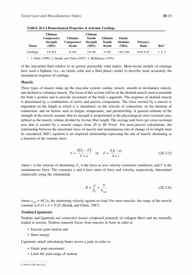
Patent Law and Miscellaneous Topics 20-19
© 1999 by CRC Press LLC
of the interstitial ßuid relative to its porous permeable solid matrix. More-recent models of cartilagehave used a biphasic (i.e., an elastic solid and a ßuid phase) model to describe more accurately themechanical response of cartilage.
Muscle
Three types of muscle make up the muscular system: cardiac muscle, smooth or involuntary muscle,and skeletal or voluntary muscle. The focus of this section will be on the skeletal muscle used to maintainthe bodyÕs posture and to provide movement of the bodyÕs segments. The response of skeletal muscleis determined by a combination of active and passive components. The force exerted by a muscle isdependent on the length at which it is stimulated, on the velocity of contraction, on the duration ofcontraction, and on factors such as fatigue, temperature, and prestretching. A general estimate of thestrength of the muscle assumes that its strength is proportional to the physiological cross-sectional area,deÞned as the muscle volume divided by its true Þber length. The average unit force per cross-sectionalarea that is exerted by a muscle ranges from 20 to 80 N/cm2. For more-precise calculations, therelationship between the maximum force of muscle and instantaneous rate of change of its length mustbe considered. HillÕs equation is an empirical relationship expressing the rate of muscle shortening asa function of the isotonic force
(20.3.5)
where v is the velocity of shortening, Fo is the force at zero velocity (isometric condition), and F is theinstantaneous force. The constants a and b have units of force and velocity, respectively, determinedempirically using the relationship
(20.3.6)
where vmax = bFo/a, the shortening velocity against no load. For most muscles, the range of the muscleconstant is 0.15 < k < 0.25 (Skalak and Chien, 1987).
Tendon/Ligaments
Tendons and ligaments are connective tissues composed primarily of collagen Þbers and are normallyloaded in tension. Tendons transmit forces from muscles to bone in order to
¥ Execute joint motion and
¥ Store energy.
Ligaments attach articulating bones across a joint in order to
¥ Guide joint movement;
¥ Limit the joint range of motion;
TABLE 20.3.3 Biomechanical Properties of Articular Cartilage
Tissue
UltimateCompressive
Strength(MPa)
UltimateCompressive
Strain
UltimateTensile
Strength(MPa)
UltimateTensileStrain
ElasticModulus
(MPa)Poisson's
Ratio Ref.a
Cartilage 5.0Ð8.0 0.136 2.8Ð40 0.182 1.63Ð220 0.42Ð0.47 1, 2, 3
a 1, Duck (1990); 2, Skalak and Chien (1987); 3, McElhaney (1976).
Vb F F
F aF
F b av
b v=
-( )+
=-
+0 0or
Ka
F
b
V= =
0 max

20-20 Section 20
© 1999 by CRC Press LLC
¥ Maintain joint congruency; and
¥ Assist in providing joint stability.
The biomechanical properties of ligaments and tendons are provided in Table 20.3.4.
The general stress-strain behavior of connective soft tissue can be represented by four distinct loadingregions (Figure 20.3.2). Region I is commonly referred to as the Òtoe regionÓ and is associated with thestraightening or alignment of the randomly ordered structural Þbers. Most physiological loading occursin this region where there is a small increase in stress for a given increase in strain. Region II characterizesthe linear region where the straightened Þbers are more uniformly loaded. The tangent to the stress-strain response curve in this linear region is frequently referred to as the elastic stiffness or tangentmodulus rather than the elastic modulus in order to emphasize that the soft tissue is not truly behavingas a perfectly elastic material. At the initiation of Region III, small ßuctuations in the stress can beobserved resulting from microfailures in the soft tissue. The Þnal loading proÞle shown in Region IVexhibits catastrophic failure of the soft tissue.
Factors Affecting Biomechanical Properties
Due to the nature of biological testing, a great deal of variability in the material properties of tissue isevident in the published literature. Unlike traditional engineering materials, there are no standardprotocols or procedures for the testing of biological materials. Although some variability can be attributedto differences in the experimental approaches undertaken by the researchers, mechanical behavior ofbiological materials can also be affected by
¥ Geometric characteristics;
¥ Loading mode (i.e., tension, compression, torsion);
¥ Rate and frequency of loading;
¥ Specimen preparation (i.e., temperature, preservation method, hydration);
¥ Age or health of specimen donor;
¥ Gender;
¥ Temperature;
¥ Anatomic location of load and specimen;
¥ Species.
TABLE 20.3.4 Biomechanical Properties of Tendon and Ligament
TissueUltimate TensileStrength (MPa)
Ultimate TensileStrain
Elastic Stiffness(MPa) Ref.a
Ligament 2.4Ð38 0.20Ð1.60 2Ð111 1, 2, 3Tendon, calcaneal 30Ð60 0.09Ð0.10 600 4, 5
a 1, Yamada (1970); 2, Skalak and Chien (1987); 3, Nahum and Melvin (1993); 4, Bronzino (1995); 5, Duck (1990).
FIGURE 20.3.2 General stress-strain behavior of connective soft tissue.
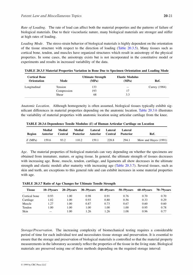
Patent Law and Miscellaneous Topics 20-21
© 1999 by CRC Press LLC
Rate of Loading. The rate of load can affect both the material properties and the patterns of failure ofbiological materials. Due to their viscoelastic nature, many biological materials are stronger and stifferat high rates of loading.
Loading Mode. The stress-strain behavior of biological materials is highly dependent on the orientationof the tissue structure with respect to the direction of loading (Table 20.3.5). Many tissues such ascortical bone, tendon, and muscles have organized structures which result in anisotropy of the physicalproperties. In some cases, the anisotropy exists but is not incorporated in the constitutive model orexperiments and results in increased variability of the data.
Anatomic Location. Although homogeneity is often assumed, biological tissues typically exhibit sig-niÞcant differences in material properties depending on the anatomic location. Table 20.3.6 illustratesthe variability of material properties with anatomic location using articular cartilage from the knee.
Age. The material properties of biological materials can vary depending on whether the specimens areobtained from immature, mature, or aging tissue. In general, the ultimate strength of tissues decreaseswith increasing age. Bone, muscle, tendon, cartilage, and ligaments all show decreases in the ultimatestrength and elastic moduli after maturity with increasing age (Table 20.3.7). Several tissues, such asskin and teeth, are exceptions to this general rule and can exhibit increases in some material propertieswith age.
Storage/Preservation. The increasing complexity of biomechanical testing requires a considerableperiod of time for each individual test and necessitates tissue storage and preservation. It is essential toensure that the storage and preservation of biological materials is controlled so that the material propertymeasurements in the laboratory accurately reßect the properties of the tissue in the living state. Biologicalmaterials are preserved using one of three methods depending on the required storage interval:
TABLE 20.3.5 Material Properties Variation in Bone Due to Specimen Orientation and Loading Mode
Cortical BoneOrientation Mode
Ultimate Strength(MPa)
Elastic Modulus(MPa) Ref.
Longitudinal Tension 133 Ñ Currey (1984)Compression 193 17Shear 68 3.3
TABLE 20.3.6 Dependence Tensile Modulus (E) of Human Articular Cartilage on Location
RegionMedial
AnteriorMedialCentral
MedialPosterior
LateralAnterior
LateralCentral
LateralPosterior Ref.
E (MPa) 159.6 93.2 110.2 159.1 228.8 294.1 Mow and Hayes (1991)
TABLE 20.3.7 Ratio of Age Changes for Ultimate Tensile Strength
Tissue 10Ð19years 20Ð29years 30Ð39years 40Ð49years 50Ð59years 60Ð69years 70Ð79years
Cortical bone 0.93 1.00 0.98 0.91 0.76 0.70 0.70Cartilage 1.02 1.00 0.93 0.80 0.56 0.33 0.29Muscle 1.27 1.00 0.87 0.73 0.67 0.60 0.60Tendon 1.00 1.00 1.00 1.00 1.00 0.95 0.78Skin Ñ 1.00 1.26 1.26 1.08 0.96 0.77

20-22 Section 20
© 1999 by CRC Press LLC
¥ Refrigeration for short-term storage;
¥ Freezing for long-term storage;
¥ Embalming for long-term storage.
Refrigeration and freezing have no effect on the properties of hard tissue. Although the effects ofrefrigeration on soft tissue properties are tissue dependent, stable properties can generally be achievedwithin 3 days of storage. Freezing of soft tissue can result in ice cavities that disrupt the tissue architectureand result in property changes. The effects of embalming on soft and hard tissue structures exhibitconßicting results.
Because many biological materials are composed primarily of water, humidity can strongly affect thestress-strain relationships (Table 20.3.8). Therefore, care must be taken to keep biological specimensmoist prior to and during testing. The control of the moisture level of specimens is most important whenanalyzing the elastic properties of surface tissues such as skin and hair. YoungÕs modulus of skin at 25to 30% relative humidity may be 1000-fold greater than that at 100% humidity (Duck, 1990).
Species. Animal tissues have been used extensively in biomechanical testing because of their availabil-ity. When extrapolating results to humans, care must be taken since signiÞcant differences can exist inthe structure and material properties between humans and other animals due to physiological andanatomic differences. Table 20.3.9 shows a comparison of elastic moduli of femoral bone specimensobtained from different animals.
Impact Biomechanics
The prevention of injury through the development of countermeasures is most effectively achievedthrough biomechanical testing and analysis. The prevalence of injuries resulting from motor vehiclecrashes, sporting activities, and industrial accidents has led to the development of a branch of biome-chanics referred to as impact biomechanics. In order to achieve the principal aims of prevention of injurythrough environmental modiÞcation, this branch of biomechanics must develop an improved understand-ing of the mechanisms of injury, descriptions of the mechanical response of the biological materialsinvolved, and information on the human tolerance to impact. Injury criteria for the human body asinterpreted by anthropometric dummies are provided in Table 20.3.10. The injury criteria are providedin terms of engineering parameters of resultant acceleration a(t), force F(t), velocity V(t), displacements(t), and anthropometric scaling factors such as the chest depth D.
Computational Biomechanics
Computational mechanics provides a versatile means of analyzing biomechanical systems. Modelinguses either rigid-body models composed of rigid masses, springs, joints, and contact surfaces or ßexible-
TABLE 20.3.8 Comparison of Material Properties between Wet and Dry Cortical Bone
TestCondition
Ultimate TensileStrength (kg/mm2)
Ultimate PercentageElongation (%)
Elastic Modulus(kg/mm2) Ref.
Wet tibia 14.3 ± 0.12 1.50 1840 Yamada (1970)Dry tibia 17.4 ± 0.12 1.38 2100 Yamada (1970)
TABLE 20.3.9 Comparison of Bone Elastic Modulus between Different Species
Tissue Source Tissue Elastic Modulus (MPa) Ref.
Human Femur 18 Currey (1984)Cow Femur 23Sheep Femur 22Tortoise Femur 10
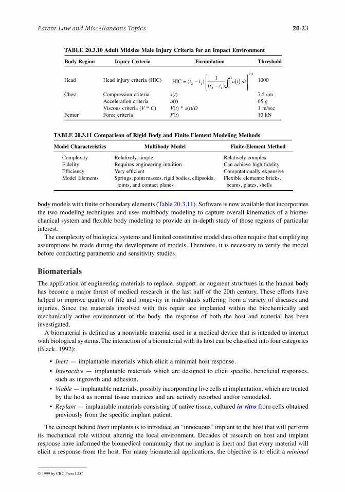
Patent Law and Miscellaneous Topics 20-23
© 1999 by CRC Press LLC
body models with Þnite or boundary elements (Table 20.3.11). Software is now available that incorporatesthe two modeling techniques and uses multibody modeling to capture overall kinematics of a biome-chanical system and ßexible body modeling to provide an in-depth study of those regions of particularinterest.
The complexity of biological systems and limited constitutive model data often require that simplifyingassumptions be made during the development of models. Therefore, it is necessary to verify the modelbefore conducting parametric and sensitivity studies.
Biomaterials
The application of engineering materials to replace, support, or augment structures in the human bodyhas become a major thrust of medical research in the last half of the 20th century. These efforts havehelped to improve quality of life and longevity in individuals suffering from a variety of diseases andinjuries. Since the materials involved with this repair are implanted within the biochemically andmechanically active environment of the body, the response of both the host and material has beeninvestigated.
A biomaterial is deÞned as a nonviable material used in a medical device that is intended to interactwith biological systems. The interaction of a biomaterial with its host can be classiÞed into four categories(Black, 1992):
¥ Inert Ñ implantable materials which elicit a minimal host response.
¥ Interactive Ñ implantable materials which are designed to elicit speciÞc, beneÞcial responses,such as ingrowth and adhesion.
¥ Viable Ñ implantable materials, possibly incorporating live cells at implantation, which are treatedby the host as normal tissue matrices and are actively resorbed and/or remodeled.
¥ Replant Ñ implantable materials consisting of native tissue, cultured in vitro from cells obtainedpreviously from the speciÞc implant patient.
The concept behind inert implants is to introduce an ÒinnocuousÓ implant to the host that will performits mechanical role without altering the local environment. Decades of research on host and implantresponse have informed the biomedical community that no implant is inert and that every material willelicit a response from the host. For many biomaterial applications, the objective is to elicit a minimal
TABLE 20.3.10 Adult Midsize Male Injury Criteria for an Impact Environment
Body Region Injury Criteria Formulation Threshold
Head Head injury criteria (HIC) 1000
Chest Compression criteria s(t) 7.5 cmAcceleration criteria a(t) 65 gViscous criteria (V * C) V(t) * s(t)/D 1 m/sec
Femur Force criteria F(t) 10 kN
TABLE 20.3.11 Comparison of Rigid Body and Finite Element Modeling Methods
Model Characteristics Multibody Model Finite-Element Method
Complexity Relatively simple Relatively complexFidelity Requires engineering intuition Can achieve high ÞdelityEfÞciency Very efÞcient Computationally expensiveModel Elements Springs, point masses, rigid bodies, ellipsoids,
joints, and contact planesFlexible elements: bricks, beams, plates, shells
HIC = --
( )é
ëêê
ù
ûúúò( )
( )
.
t tt t
a t dtt
t
2 12 1
2 51
1
2

20-24 Section 20
© 1999 by CRC Press LLC
host response. Those implants that are interactive with the biological environment do so in a desiredand planned fashion. Viable implants are at their infancy, but already show promise in assisting andpossibly directing tissue repair. The concept of an entire organ replant is still unrealized, but currentstrides in deciphering the human genetic code will make replants of autologous materials a clinicalmethod of the future.
Material and Host Response
The Physiological Environment. The Þrst reaction of the body to an implant is to Òwall offÓ or builda Þbrous tissue capsule around the implant. The biomaterial will be enclosed in a Þbrous capsule ofvarying tissue thickness that will depend on the material and the amount of motion between the tissuesand the implant. When the biomaterial elicits a minimal encapsulating response, it is possible for thetissue to integrate with the implant mechanically. This has been demonstrated in total-joint replacementwhen new bone is formed to interdigitate with a porous surface. Another approach to biocompatibilityhas been to use the tissue response to a material to beneÞt the function of the implant. This approachis used when bone chemically bonds to the hydroxyapetite coatings on hip implants.
The interaction between implant material and the host occurs at both the chemical and mechanicallevel. There are several parameters that affect the response of the biomaterial to the host environmentand the overall performance:
¥ The pH and salt content of the implant site Ñ A Pourbaix diagram for saline environments shouldbe consulted to see if the metal will be passivated.
¥ Lipid content of the implant site Ñ Lipophilic materials may swell or lose strength.
¥ Mechanical environment Ñ Implant materials may wear, creep, and/or fatigue.
¥ Corrosive potential of the material Ñ Metallic implants are susceptible to galvanic, crevice, andother types of corrosion.
¥ Method of manufacture and handling Ñ Scratches and other defects will increase the likelihoodof crack development and/or crevice corrosion.
¥ Method of sterilization Ñ Some methods of sterilization will cross-link polymers or affect thedegradation of biodegradable materials.
The host response to an implanted material is also affected by both chemical and mechanical factors.A few parameters that affect host response are
¥ Leached materials from the implant Ñ Leached material, consisting of metallic ions, polymericmolecules, or solvents from manufacturing, may denature proteins. The pathway and effects ofleached material should be examined.
¥ Surface tension and electric charge of the material.
¥ Stiffness of the biomaterial Ñ Stress shielding of the bone by a stiff implant has been shown toaffect bone remodeling.
¥ Geometry of the implant Ñ Sharp edges have been shown to increase the Þbrous tissue capsulethickness.
¥ Method of cleaning and sterilization Ñ Solvents, Þlings, or residues left from the manufacturing,handling, or sterilization processes will likely cause unwanted host response and increase theprobability of infection.
The expected life span of an implant varies with application. Some implants are used for temporarystructural support, such as intermedullary nails for fracture Þxation. In this application, corrosion is notas critical an issue as cost and mechanical fatigue. Another approach to temporary applications has beenthe use of biodegradable materials that eventually dissolve into the body. Biodegradable materials havebeen used for fracture Þxation and drug delivery with success.

Patent Law and Miscellaneous Topics 20-25
© 1999 by CRC Press LLC
Current Biomaterials
Metallic Biomaterials. Metals are typically selected for biomedical applications because of their hightensile strength (Table 20.3.12). With the high tensile strength of metals comes a high elastic modulusthat can lead to stress shielding of the bone. Bone, which remodels in response to its loading environment,resorbs in regions of low stress which can lead to implant loosening.
Another issue when using metals in the body is corrosion since very few metals are in a passivatedstate while in vivo. Metallic implant materials are subject to several types of corrosion: galvanic, crevice,pitting, intergranular, and stress/fatigue. For metallic biomaterial selection, it is best to refer to thecorrosion potential of a material in seawater, rather than tap water since seawater is a reasonableapproximation for the in vivo environment. Implant designs that involve dissimilar metals or multiplepieces have increased susceptibility to galvanic corrosion (Cook et al., 1985). A reasonable predictionof the reactivity between dissimilar metals can be made upon consideration of the galvanic series.
Polymers. The number of polymers available for biomedical applications has been increasing rapidlyin the last few decades. Polymers are viscoelastic materials whose mechanical properties, host response,and material response depend on molecular weight, degree of cross-linking, temperature, and loadingrate, among other factors. Therefore, it should be recognized that tabular data representing the mechanicalproperties of polymers only indicates the general range of properties for a class of polymers (Tables20.3.13 and 20.3.14). Common applications of polymers in biomedical engineering include articularwear components, drug-delivery devices, cosmetic augmentation, blood vessels, and structural applica-tions.
Biodegradable Polymers. There are a plethora of degradable polymers available to the modern bio-medical engineer. Each is unique in mechanical properties, degradation time, degradation products, andsensitivity of strength to degradation. Recent efforts in polymer development have focused on biode-gradable materials that serve as either temporary support or drug-delivery devices during the healing
TABLE 20.3.12 Common Metallic Biomaterials
Metal FormDensity(g/cm3)
EModulus
(GPa)
YieldStrength(MPa)
FatigueStrength @107 Cycles
(MPa) CharacteristicsMedical
Applications Ref.a
Ti-6Al-4V
ANCP-Ti
4.4Ñ
127120
830Ð896470
620Ñ
Chemically inert, poor wear properties, good fatigue properties, high strength-to-weight ratio, closest modulus to that of bone
Total hip and knee stems
1, 5
Co-Cr-Mo, ASTM F-75
C/ANW/AN
7.89.15
200230
450Ð492390
207Ð310Ñ
Excellent wear properties, castable, Co and Cr ions have been found mutagenic in vitro
Articular surfaces in hips and knees, dental implants, hip stems
2, 3
AISI-316LVMStainless
AN30%CW
7.9Ñ
210230
211Ð280750Ð1160
190Ð230530Ð700
Inexpensive Temporary applications, bone screws, bone plates, suture
5Ð7
Tantalum CW 16.6 190 345 Ñ Very inert, very dense Transdermal implant testing, suture
4
Note: AN: annealed, CW: cold worked, C: cast, W: wrought, CP: chemically pure.a 1, ASTM F136-79; 2, ASTM F75-82; 3, ASTM F90-82; 4, ASTM F560-86, p. 143, 1992; 5, Green and Nokes (1988);
6, ASTM F55-82; 7, Smith and Hughes (1977).
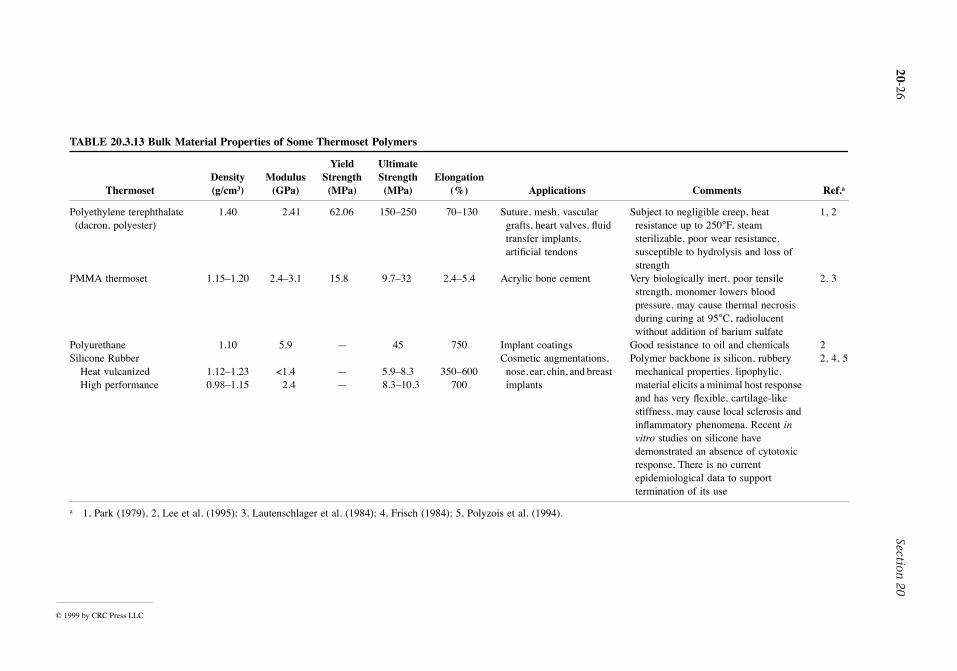
20-26Section
20
© 1999 by CRC Press LLC
TABLE 20.3.13 Bulk Material Properties of Some Thermoset Polymers
ThermosetDensity(g/cm3)
Modulus(GPa)
YieldStrength(MPa)
UltimateStrength(MPa)
Elongation(%) Applications Comments Ref.a
Polyethylene terephthalate (dacron, polyester)
1.40 2.41 62.06 150Ð250 70Ð130 Suture, mesh, vascular grafts, heart valves, ßuid transfer implants, artiÞcial tendons
Subject to negligible creep, heat resistance up to 250°F, steam sterilizable, poor wear resistance, susceptible to hydrolysis and loss of strength
1, 2
PMMA thermoset 1.15Ð1.20 2.4Ð3.1 15.8 9.7Ð32 2.4Ð5.4 Acrylic bone cement Very biologically inert, poor tensile strength, monomer lowers blood pressure, may cause thermal necrosis during curing at 95°C, radiolucent without addition of barium sulfate
2, 3
Polyurethane 1.10 5.9 Ñ 45 750 Implant coatings Good resistance to oil and chemicals 2Silicone Rubber Cosmetic augmentations,
nose, ear, chin, and breast implants
Polymer backbone is silicon, rubbery mechanical properties, lipophylic, material elicits a minimal host response and has very ßexible, cartilage-like stiffness, may cause local sclerosis and inßammatory phenomena. Recent in vitro studies on silicone have demonstrated an absence of cytotoxic response. There is no current epidemiological data to support termination of its use
2, 4, 5Heat vulcanizedHigh performance
1.12Ð1.230.98Ð1.15
<1.42.4
ÑÑ
5.9Ð8.38.3Ð10.3
350Ð600700
a 1, Park (1979), 2, Lee et al. (1995); 3, Lautenschlager et al. (1984); 4, Frisch (1984); 5, Polyzois et al. (1994).

Paten
t Law
and
Miscellan
eous Topics
20-27
© 1999 by CRC Press LLC
TABLE 20.3.14 Thermoplastic Biomedical Polymers
ThermoplasticDensity(g/cm3)
Modulus(GPa)
YieldStrength(MPa)
UltimateStrength(MPa)
Tglass
(°C)Elongation
(%) Applications Comments Ref.a
PMMA thermoplastic 1.19 2.4Ð3.1 Ñ 50Ð75 105 2Ð10 Contact lenses, blood pump
Very biologically inert, excellent optical properties, radiolucent without barium sulfate added, losses strength when heat sterilized
1Ð3
Polypropylene 0.85Ð0.98 1.5 Ñ 30Ð40 Ð12 50Ð500 Disposable syrine, suture, artiÞcial vascular grafts
High ßex life, excellent environment stress cracking resistance
2, 1
Polyvinylchloride (PVC) rigid
1.35Ð1.45 3.0 Ñ 40Ð55 70Ð105 400 Blood and solution bags, catheters, dialysis devices
High melt viscosity, thus difÞcult to process
2, 1
Polysulfone 1.23Ð1.25 2.3Ð2.48 65Ð96 106 Ñ 20Ð75 Hemodialysis, artiÞcial kidney circulatory assist, composite matrix
High thermal stability and chemical stability, unstable in polar organic solvents such as ketones or chlorinated hydrocarbons
2, 3
Polytetra-ßouroethylene (Teßon)
2.15Ð2.20 0.5Ð1.17 Ñ 17Ð28 Ñ 320Ð350 Catheter, artiÞcial vascular grafts
Heat sterilizable, low coefÞcient of friction, not recommended as a bearing surface, inert in solid form
1, 5
UHMWPE molded and machined extruded
0.93Ð0.970.93Ð0.94
Ñ1.24
2121Ð28
3434Ð47
ÑÑ
300200Ð250
Articular bearing surfaces UHMW has MW > 2E6 g/mol, very inert, induces minimal swelling in vivo, high concentration of wear particles leads to bone resorbtion, creeps under load, has heat resistance up to 180°F which is too low for steam sterilization
4
a 1, Park (1979); 2, Lee et al. (1995); 3, Dunkle (1988); 4, ASTM 648-83; 5, ASTM F754.
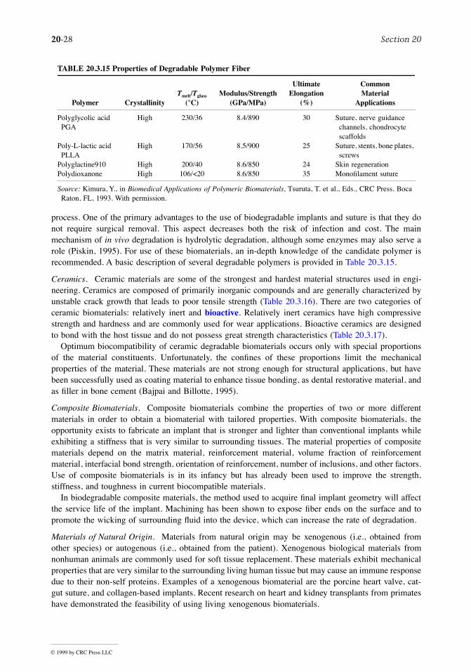
20-28 Section 20
© 1999 by CRC Press LLC
process. One of the primary advantages to the use of biodegradable implants and suture is that they donot require surgical removal. This aspect decreases both the risk of infection and cost. The mainmechanism of in vivo degradation is hydrolytic degradation, although some enzymes may also serve arole (Piskin, 1995). For use of these biomaterials, an in-depth knowledge of the candidate polymer isrecommended. A basic description of several degradable polymers is provided in Table 20.3.15.
Ceramics. Ceramic materials are some of the strongest and hardest material structures used in engi-neering. Ceramics are composed of primarily inorganic compounds and are generally characterized byunstable crack growth that leads to poor tensile strength (Table 20.3.16). There are two categories ofceramic biomaterials: relatively inert and bioactive. Relatively inert ceramics have high compressivestrength and hardness and are commonly used for wear applications. Bioactive ceramics are designedto bond with the host tissue and do not possess great strength characteristics (Table 20.3.17).
Optimum biocompatibility of ceramic degradable biomaterials occurs only with special proportionsof the material constituents. Unfortunately, the conÞnes of these proportions limit the mechanicalproperties of the material. These materials are not strong enough for structural applications, but havebeen successfully used as coating material to enhance tissue bonding, as dental restorative material, andas Þller in bone cement (Bajpai and Billotte, 1995).
Composite Biomaterials. Composite biomaterials combine the properties of two or more differentmaterials in order to obtain a biomaterial with tailored properties. With composite biomaterials, theopportunity exists to fabricate an implant that is stronger and lighter than conventional implants whileexhibiting a stiffness that is very similar to surrounding tissues. The material properties of compositematerials depend on the matrix material, reinforcement material, volume fraction of reinforcementmaterial, interfacial bond strength, orientation of reinforcement, number of inclusions, and other factors.Use of composite biomaterials is in its infancy but has already been used to improve the strength,stiffness, and toughness in current biocompatible materials.
In biodegradable composite materials, the method used to acquire Þnal implant geometry will affectthe service life of the implant. Machining has been shown to expose Þber ends on the surface and topromote the wicking of surrounding ßuid into the device, which can increase the rate of degradation.
Materials of Natural Origin. Materials from natural origin may be xenogenous (i.e., obtained fromother species) or autogenous (i.e., obtained from the patient). Xenogenous biological materials fromnonhuman animals are commonly used for soft tissue replacement. These materials exhibit mechanicalproperties that are very similar to the surrounding living human tissue but may cause an immune responsedue to their non-self proteins. Examples of a xenogenous biomaterial are the porcine heart valve, cat-gut suture, and collagen-based implants. Recent research on heart and kidney transplants from primateshave demonstrated the feasibility of using living xenogenous biomaterials.
TABLE 20.3.15 Properties of Degradable Polymer Fiber
Polymer CrystallinityTmelt/Tglass
(°C)Modulus/Strength
(GPa/MPa)
UltimateElongation
(%)
CommonMaterial
Applications
Polyglycolic acid PGA
High 230/36 8.4/890 30 Suture, nerve guidance channels, chondrocyte scaffolds
Poly-L-lactic acid PLLA
High 170/56 8.5/900 25 Suture, stents, bone plates, screws
Polyglactine910 High 200/40 8.6/850 24 Skin regenerationPolydioxanone High 106/<20 8.6/850 35 MonoÞlament suture
Source: Kimura, Y., in Biomedical Applications of Polymeric Biomaterials, Tsuruta, T. et al., Eds., CRC Press, Boca Raton, FL, 1993. With permission.
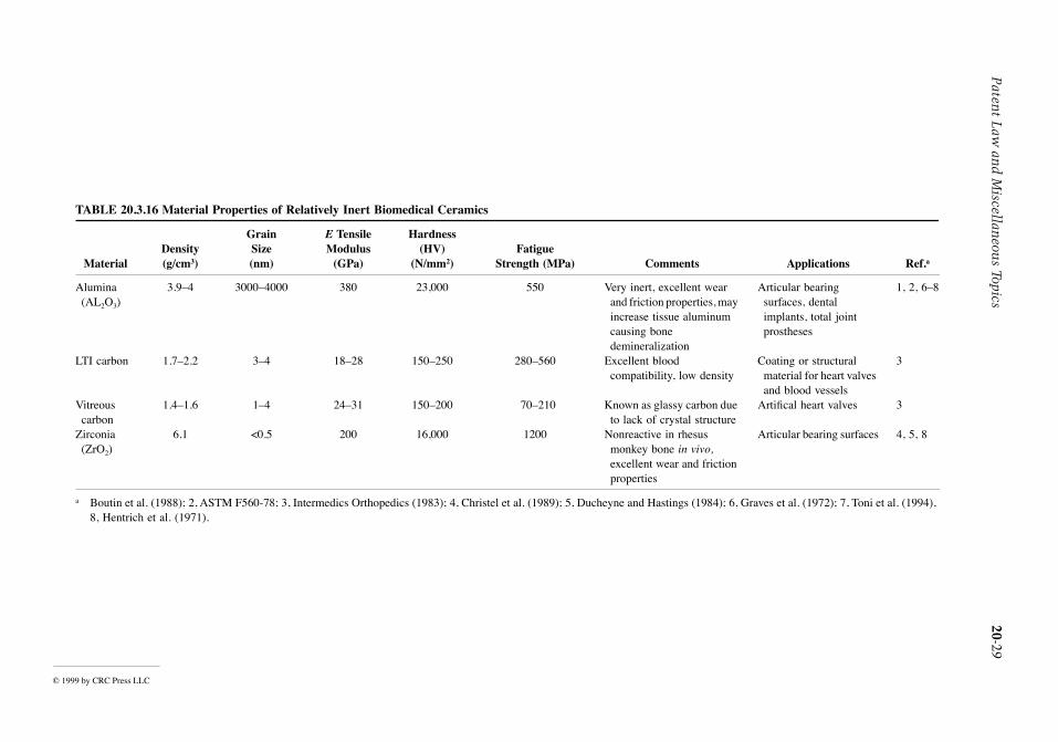
Paten
t Law
and
Miscellan
eous Topics
20-29
© 1999 by CRC Press LLC
TABLE 20.3.16 Material Properties of Relatively Inert Biomedical Ceramics
MaterialDensity(g/cm3)
GrainSize(nm)
E TensileModulus
(GPa)
Hardness(HV)
(N/mm2)Fatigue
Strength (MPa) Comments Applications Ref.a
Alumina (AL2O3)
3.9Ð4 3000Ð4000 380 23,000 550 Very inert, excellent wear and friction properties, may increase tissue aluminum causing bone demineralization
Articular bearing surfaces, dental implants, total joint prostheses
1, 2, 6Ð8
LTI carbon 1.7Ð2.2 3Ð4 18Ð28 150Ð250 280Ð560 Excellent blood compatibility, low density
Coating or structural material for heart valves and blood vessels
3
Vitreous carbon
1.4Ð1.6 1Ð4 24Ð31 150Ð200 70Ð210 Known as glassy carbon due to lack of crystal structure
ArtiÞcal heart valves 3
Zirconia (ZrO2)
6.1 <0.5 200 16,000 1200 Nonreactive in rhesus monkey bone in vivo, excellent wear and friction properties
Articular bearing surfaces 4, 5, 8
a Boutin et al. (1988); 2, ASTM F560-78; 3, Intermedics Orthopedics (1983); 4, Christel et al. (1989); 5, Ducheyne and Hastings (1984); 6, Graves et al. (1972); 7, Toni et al. (1994), 8, Hentrich et al. (1971).

20-30 Section 20
© 1999 by CRC Press LLC
Autogenous materials are used when skin and bone are relocated on a patient. As human ability tomanipulate the human genetic code continues, it may be possible to replace failed human organs withidentical organs that have been grown either in vitro or in vivo.
Biomaterial Testing
The human body is a biologically and mechanically active environment that reacts to all materials.Biomaterials should be initially selected for their engineering mechanical properties to serve a speciÞcfunction. Careful consideration must be given to the fatigue and creep properties of the material becauseof the rigorous loading incurred by many implants. The anterior cruciate ligament of a moderately activeperson, for example, will be subjected to 4.2 million loading cycles annually (Black, 1992). Thisfrequency of cyclic loading is consistent with the cyclic loading of other orthopedic structures.
Once a candidate material has been selected, the material must be tested to determine both the materialresponse to its proposed biological environment and the host response to that material. Valuable hostand material response information may be obtained from the use of in vitro tests that simulate a speciÞcphysiological environment. The Þnal step before implantation into a human is to test the performanceof a candidate material with an animal model.
In Vitro Studies. Experimental in vitro studies should be conducted prior to testing on living animals.In vitro studies provide essential information on the response of the candidate biomaterials to a simulatedhost environment and on the chemical interactions that ensue. It is important to observe the effect ofthe biomaterial on proteins to determine if any coating, denaturing, or other processes result. Thesestudies are inexpensive and can be tailored to simulate speciÞc implant sites. Initial tests may simplyexpose the candidate material to the expected inorganic chemical and thermal conditions. More complexin vitro tests may include appropriate, viable, active cells with their associated cell products. The cellsurvival count, reproduction rate, metabolic activity, effective motion activity, and cell damage shouldbe observed during testing (Black, 1992). Some sample in vitro materials tests are described in Table20.3.18.
Biomaterials intended for vascular applications must be tested for their interaction with blood. Exam-ination of blood-biomaterial interactions should include protein absorption, platelet interactions, intrinsiccoagulation, Þbrinolytic activity, erythrocytes, leukocytes, and complement activation. Since the circu-latory system has both an oxygen- and nutrient-rich arterial side and a carbon dioxide-rich venous side,a candidate material must be tested in the environment for which it is intended.
In Vivo Studies. Animal studies are extremely valuable for examining the host and material responseof a speciÞc test material. These studies must be in complete accordance with the Animal Welfare Act(7 U.S.C. 2131, December 23, 1985). Initial animal tests are nonfunctional and involve placing a testspecimen in an anatomic location similar to the expected implant location. These locations may besubcutaneous, intramuscular, intraperitoneal, transcortical, or intramedullar. Depending on the study, theduration of implantation can vary from weeks to years. Factors that affect the outcome of nonfunctional
TABLE 20.3.17 Bioactive Ceramic Materials
Material Chemical Content Comments Ref.a
Hydroxyapatite Ca10(PO4)6(OH)2 Actual mineral phase of bone, used as a coating or solid, synthetic versions available, good mechanical properties, excellent biocompatibility, subject to osteoclastic resorbtion, chemically bonds to bone
1, 2
Bioglass 46S5.2 46.1% SiO2, 26.9% CaO, 24.4% Na2O, 2.6% P2O5 mol%
Fine-grained, glassy ceramics, 46S5.2 exhibits best tissue bonding, other constitutent ratios are available
3, 4
Ceravital Bioglass materials with Al2O3, TiO2, and Ta2O5 added
Very similar composition to bioglass with additional metal oxides to control dissolution rate
4
a 1, Gessink et al. (1987); 2, Kay (1988); 3, Hench and Ethridge (1982); 4, Bajpai and Billotte (1995).

Patent Law and Miscellaneous Topics 20-31
© 1999 by CRC Press LLC
tests include the degree of relative motion between implant and host and the geometry of the testspecimen.
Functional testing of biomedical materials is performed in order to evaluate a test material or designas it performs its intended function. Species are selected for an animal model based on similarities withhuman models and then scaled to size. Some factors to consider are the life span, activity level, metabolicrate, and size of the test animal. Results are determined from macroscopic and histological evaluations.
Defining Terms
Autologous: Related to self; materials obtained from the same organism.Bioactive: The ability of a material to chemically interact with the host environment in a predetermined
manner.Biocompatibility: The ability of a biomaterial to perform with an appropriate host response in a speciÞc
manner.Bioengineering: The application of principles from engineering, applied mathematics, and physics to
the study of biological problems.Biomaterial: A nonviable material used in a medical device that is intended to interact with biological
systems.Biomechanics: The study of forces that act on and within a biological structure and the effects that
these forces produce.In vitro: Within a glass; observable in an artiÞcial environment such as a test tube.In vivo: Within the living body.Remodeling: Changes in internal architecture and external conformation of biological tissues in accor-
dance with applied strain.Sterilization: The complete elimination or destruction of all living microorganisms. The most common
methods are steam, radiation, and chemical sterilization.
References
Bajpai, P.K. and Billotte, W.G. 1995. Ceramic biomaterials; in The Biomedical Engineering Handbook,J.D. Bronzino, Ed., CRC Press, Boca Raton, FL, chap. 41, 552Ð580.
Black, J. 1992. Biological Performance of Materials; Fundamentals of Biocompatibility, Marcel Dekker,New York.
Boutin, P., Christel, P., Dorlot, J.M., Meunir, A., de Roquancourt, A., Blanquaert, D., Herman, S., Sedel,L., and Witvoet, J. 1988. J. Biomed. Mater. Res., 22,1203.
Bronzino, J.D., Ed. 1995. The Biomedical Engineering Handbook, CRC Press, Boca Raton, FL.Christel, P., Meunier, A., Heller, M., Torre, J.P., and Peille, C.N. 1989. J. Biomed. Mater. Res., 23, 45.
TABLE 20.3.18 Sample In Vitro Tests
In Vitro Test Brief Description
ASTM F895-4 cytotoxicity
Place sterile agar over mouse Þbroblast cells. Place the test material on top and incubate for 24 hr; examine the culture for the extent of cell lysis
Ames test for mutagenicity
Expose autotrophic Salmonella typhinurium bacteria cells to the test material and histidine for 48 hr at 37°C; if cells mutate to non-autotrophic state, histidine levels will be lower after testing
LeeÐWhite coagulation rate
Place a small volume of fresh-drawn blood on a test surface and similar amount on control surface; compare coagulation times
Ex vivo blood compatibility
Tap into the bloodstream of a canine; let blood ßow at typical rates and pressure through a test specimen for a short time; examine specimen for platelet adhesion and blood for hemolysis

20-32 Section 20
© 1999 by CRC Press LLC
Cook, S.D., Renz, E.A., Barrack, R.L., Thomas, K.A., Harding, A.F., Haddad, R.J., and Milicic, M.1985. Clin. Orthop., 194(236).
Cowin, S.C. 1989. Bone Mechanics, CRC Press, Inc., Boca Raton, FL.Currey, J.D. 1984. Mechanical Adaptations of Bone, Princeton University Press, Princeton, NJ.Ducheyne, P. and Hastings, G.W., Eds. 1984. Metal and Ceramic Biomaterials, CRC Press, Boca Raton,
FL.Duck, F. 1990. Physical Properties of Tissue, Academic Press, San Diego, CA.Dunkle, S.R. 1988. Engineering plastics, in Engineered Materials Handbook, Vol. 2, C.A. Dostal, Ed.,
ASM Int., Metals Park, OH, 200ff.Frisch, E. 1984. Polymeric materials and artiÞcial organs, in ACS Symposium 256, C.G. Gebelein, Ed.,
American Chemical Society, Washington, D.C., 63ff.Fung, Y.C. 1993. Biomechanics: Mechanical Properties of Living Tissues, 2nd ed. Springler-Verlag, New
York.Gessink, R.G., deGroot, K., and Klein, C. 1987. Chemical implant Þxation using hydroxyapatite coatings,
Clin. Orthop. Relat. Res., 226(147).Green, M. and Nokes, L.D.M., Eds. 1988. Engineering Theory in Orthopaedics: An Introduction, Ellis
Horwood, Chichester, England.Hench, L.L. and Ethridge, E.C. 1982. Biomaterials: An Interfacial Approach, Academic Press, New York.Kay, J.F. 1988. Bioactive surface coatings: cause for encouragement and caution, J. Oral Implantol.,
16(43).Kimura, Y. 1993. Biomedical polymers, in Biomedical Applications of Polymeric Biomaterials, T.
Tsuruta, T. Hayashi, K. Kataoka et al., Eds., CRC Press, Boca Raton, FL.Lautenschlager, E.P., Stupp, S., and Keller, J.C. 1984. In Functional Behavior of Orthopedic Biomate-
rials, Vol. II., P. Ducheyne and G.W. Hastings, Eds., CRC Press, Boca Raton, FL, 87ff.Lee, H.B., Kim, S.S., and Khang, G. 1995. Polymeric biomaterials, in The Biomedical Engineering
Handbook, J.D. Bronzino, Ed., CRC Press, Boca Raton, FL, 581Ð597.McElhaney, J.H., Roberts, V.L., and Hilyard, J.F., 1976. Handbook of Human Tolerance, Japanese
Automobile Research Institute, Tokyo, Japan.Mow, V.C. and Hayes, V.C. 1991. Basic Orthopedic Biomechanics, Raven Press, New York.Nahum, A.M. and Melvin, J.W., Eds. 1993. Accidental Injury: Biomechanics and Prevention, Springler-
Verlag, New York.Nigg, B.M. and Herzog, W., Eds. 1994. Biomechanics of the Musculo-Skeletal System, John Wiley and
Sons, Chichester, England.Nordin, M. and Frankel, V.H. 1989. Basic Biomechanics of the Musculoskeletal System, Lea and Febiger,
Malvern, PA.Park, J.B. 1979. Biomaterials: An Introduction, Plenum Press, New York.Piskin, E. 1995. Biodegradable polymers as biomaterials, J. Biomat. Sci. Polym. Ed. 6(9), 775Ð795.Polyzois, G.L., Hensten-Pettersen, A., and Kullmann, A. 1994. An assessment of the physical properties
and biocompatibility of three silicone elastomers, J. Prosth. Dent. 71(5), 500-504.Skalak, R. and Chien, S. 1987. Handbook of Bioengineering, McGraw-Hill, New York.Smith, D.J.E. and Hughes, A.N. 1977. The inßuence of frequency and cold work on fatigue strength of
316L stainless steel in air and 0.17M saline, AWRE Rep., 44/83/189, Atomic Weapons ResearchEstablishment, Aldermaston, Berkshire, U.K.
Yamada, H. 1970. In Strength of Biological Materials, F.G. Evans, Ed., Williams and Wilkins, Baltimore,MD.

Patent Law and Miscellaneous Topics 20-33
© 1999 by CRC Press LLC
Further Information
A comprehensive summary of the biomechanical properties of tissues can be found in the Strength ofBiological Materials (Yamada, 1970). A good introduction to material response, material testing, andhost response is presented in Biological Performance of Materials; Fundamentals of Biocompatibility(Black, 1992).
A reference that goes more in-depth on biomaterial chemical contents, applications, and manufacturingis The Biomedical Engineering Handbook, edited by Joseph Bronzino (1995).
The Journal of Biomedical Materials Research is a monthly publication that reports advancementsin the Þeld of biomaterial development and testing. For subscription information contact: Journal ofBiomedical Materials Research, Subscription FulÞllment and Distribution, John Wiley and Sons, Inc.,605 3rd Avenue, New York, NY 10158.
The Journal of Biomechanics covers a wide range of topics in biomechanics, including cardiovascular,respiratory, dental, injury, orthopedic, rehabilitation, sports, and cellular. For subscription information,contact: Elsevier Science, Inc., 660 White Plains Road, Tarrytown, NY 10591-5153.

20-34 Section 20
© 1999 by CRC Press LLC
20.4 Mechanical Engineering Codes and Standards
Michael Merker
What Are Codes and Standards?
A standard can be deÞned as a set of technical deÞnitions, requirements, and guidelines for the uniformmanufacture of items; safety, and/or interchangeability. A code is a standard which is, or is intended tobe, adopted by governmental bodies as one means of satisfying legislation or regulation. Simply put,they can range from a general set of minimum requirements to very speciÞc Òhow toÓ instructions fordesigners and manufacturers.
Voluntary standards, and they can run from a few paragraphs to hundreds of pages, are written byexperts who sit on the many committees administered by standards-developing organizations (SDOs),such as ASME International.
They are not considered voluntary because they are created by volunteers; rather they are voluntarybecause they serve as guidelines, but do not of themselves have the force of law. ASME Internationalpublishes its standards; accredits users of standards to ensure that they have the capability of manufac-turing products that meet those standards; and provides a stamp that accredited manufacturers may placeon their product, indicating that it was manufactured according to the standard. ASME Internationalcannot, however, force any manufacturer, inspector, or installer to follow ASME International standards.Their use is voluntary.
Why are voluntary standards effective? Perhaps the American Society for Testing and Materials(ASTM) said it best in its 1991 annual report. ÒStandards are a vehicle of communication for producersand users. They serve as a common language, deÞning quality and establishing safety criteria. Costs arelower if procedures are standardized; training is also simpliÞed. And consumers accept products morereadily when they can be judged on intrinsic merit.Ó
A dramatic example of the value and impact codes and standards have had on our society is providedby ASME InternationalÕs Boiler and Pressure Vessel Code. Toward the end of the 19th century, boilersof every description, on land and at sea, were exploding with terrifying regularity for want of reliablytested materials, secure Þttings, and proper valves. They would continue to do so into the 20th century.Engineers could take pride in the growing superiority of American technology, but they could not ignorethe price of 50,000 dead and 2 million injured by accidents annually.
The mechanical engineers who tackled the problems in 1884 began by seeking reliable methods fortesting steam boilers. The need for the establishment of universally accepted construction standardswould take many more years and resulted in the Þrst edition of the Boiler and Pressure Vessel Codebeing published by ASME International in 1915.
Codes and Standards–Related Accreditation, Certification, and Registration Programs
Accreditation
Shortly after the Boiler Code was Þrst published, the need emerged for a recognizable symbol to beafÞxed to a product constructed in accordance with the standards. ASME International commissionedappropriate seals that are now the internationally acknowledged symbols of the Society. The symbol isstamped onto the product.
But how does a manufacturer obtain permission to use one of the symbols? Through the ASMEInternational accreditation process, the manufacturer's quality control process is reviewed by an ASMEInternational team. If the quality control system meets the requirements of the applicable ASMEInternational code or standard and the manufacturer successfully demonstrates implementation of theprogram, the manufacturer is accredited by ASME International. This means that the manufacturer maycertify the product as meeting ASME International standards and may apply the stamp to the product.

Patent Law and Miscellaneous Topics 20-35
© 1999 by CRC Press LLC
The stamp consists of a modiÞed cloverleaf (from the shape of the ASME International logo), withletter(s) in the center. The letter(s) indicate the code or section of the code met by the product uponwhich it is placed. Boiler and pressure vessel stamps issued are
A Field Assembly of Power Boilers,E Electric Boilers,H Heating Boilers, Steel Plate, or Cast-Iron Sectional,HV Heating Boiler Safety Valves,HLW Lined Potable Water Heaters,M Miniature Boilers,N Nuclear Components,NPT Nuclear Component Partial,NA Nuclear Installation/Assembly,NV Nuclear Safety Valves,PP Pressure Piping,RP Reinforced Plastic Pressure Vessels,S Power Boilers,U, U2 Pressure Vessels,UM Miniature Pressure Vessels,UV Pressure Vessel Safety Valves,V Boiler Safety Valves.
ASME International also has accreditation programs for nuclear materials, offshore safety and pol-lution prevention equipment, fasteners, authorized inspection agencies, organizations that certify elevatorinspectors, and reinforced thermoset plastic corrosion-resistant vessels.
Certification
ASME International has also expanded its scope of activity to cover certiÞcation of individuals. TheÞrst program became available in 1992 and covered the qualiÞcation and certiÞcation of resource recoveryfacilities operators. They have since added programs to cover operators of hazardous waste incineratorsand medical waste incinerators. Programs to certify an individual's knowledge and ability in the area ofgeometric dimensioning and tolerancing and operators of fossil fuelÐÞred plants are under development.
Registration
Registration is similar to accreditation; however, it is the term used more frequently in the internationalarena, particularly when dealing with the International Organization for Standardization (ISO) 9000program on quality assurance systems. ASME InternationalÕs ISO 9000 Registration Program has beenaccredited by the American National Accreditation Program for Registrars of Quality Systems (ANSI-RAB) and the Dutch Council for CertiÞcation (RvC) in the following industrial sectors:
Primary Metals IndustriesFabricated Metal ProductsIndustrial and Commercial Machinery and EquipmentReinforced Thermoset Plastic Tanks and VesselsEngineering Services
How Do I Get Codes and Standards?
Role of ASME International in Mechanical Engineering Standards
ASME International is a nonproÞt educational and technical organization with more than 125,000members, most of whom are practicing engineers. About 20,000 are students. ASME International hasa wide variety of programs: publishing, technical conferences and exhibits, engineering education,

20-36 Section 20
© 1999 by CRC Press LLC
government relations, and public education, as well as the development of codes and standards, all aimedat serving the engineering profession, the public, industry, and government.
The ASME International Board of Governors has delegated the codes and standards activity to a 22-member Council on Codes and Standards, which directs all aspects of the program. Under the Councilare ten boards, also made up of ASME International members and other interested persons; supervisoryboards in turn oversee committees, each responsible for a speciÞc area of standard development.
Committees in one form or another have dealt with standards since the Þrst test code in 1884. Currently,there are more than 100 main committees dealing with over 500 standards that are under regular reviewand revision. Once a standard is accepted, it is printed and made available to manufacturers, regulatoryagencies, designers Ñ anyone with an interest in that particular subject. Close to 4000 individuals serveon these committees and their subcommittees, subgroups, and working groups.
After a standard has been considered and reconsidered at meetings and through many drafts, it is sentto the main committee, representing all interests, which votes on the standard. But this is not the Þnalstep. Before the draft becomes a standard and is published and ready for distribution, it is made availablefor public comment and must be approved by the appropriate ASME International supervisory board.This process is illustrated graphically in Figure 20.4.1.
ASME International has been a consistent supporter of the policy of prior announcement of meetings,open meeting rooms, balanced committees, public announcements and reviews, appeal mechanisms,and overall procedural due process.
Role of ANSI in These and Other Related Standards
In 1911, ASME International was one of a number of organizations which recommended the establish-ment of an organization to help eliminate conßict and duplication in the development of voluntarystandards in the U.S. Such an organization was formed in 1918 and is currently known as the AmericanNational Standards Institute (ANSI). ANSI is the U.S. member of the ISO and the administrator of theU.S. National Committee of the International Electrotechnical Committee (IEC). ANSI also serves as abookseller of domestic and international standards.
The intent of obtaining ANSI approval of a standard is to verify that in establishing the standard, theoriginating organization has followed principles of openness and due process and has achieved aconsensus of those directly affected by the standard.
FIGURE 20.4.1 A typical path for standards approval.

Patent Law and Miscellaneous Topics 20-37
© 1999 by CRC Press LLC
What Standards Are Available?
Listing of Topics Covered by ASME International Standards
AbbreviationsAccreditationAir Cooled Heat ExchangersAir Cylinders & AdaptersAir HeatersAtmospheric Water Cooling EquipmentAutomatically Fired BoilersAutomotive Lifting DevicesBackwater ValvesBoilersBoltsBuilding Services PipingCablewaysCargo ContainersCarriersCastings and ForgingsCentrifugal PumpsChemical Plant and Petroleum ReÞnery
EquipmentChucks and Chuck JawsCleanoutsCoal PulverizersCompressorsConsumable ToolsConveyorsCoordinate Measuring MachinesCranesDeaeratorsDensity DeterminationDerricksDial IndicatorsDiaphragm SealsDiesDiesel and Burner FuelsDigital SystemsDimensional MetrologyDimensioning and TolerancingDraftingDrainsDumbwaitersEjectorsElevatorsEscalatorsExhaustersFansFastenersFeedwater HeatersFittings
FlangesFloor DrainsFlue Gas DesulfurizationFluid Flow in PipesFuel Gas PipingGage BlanksGage BlocksGas Flow MeasurementGas Transmission and Distribution Piping
SystemsGas Turbine Power PlantsGas TurbinesGaseous FuelsGasketsGaugesGraphic SymbolsHand ToolsHigh Lift TrucksHoistsHooksHydroelectric EquipmentIncineratorsIndicated PowerIndustrial SoundIndustrial Trucks and VehiclesInternal Combustion Engine Generator
UnitsIon Exchange EquipmentJacksKeysKeyseatsKnurlingLetter SymbolsLiftsLimits and FitsLine Conventions and LetteringLinear MeasurementsLiquid Transportation SystemsLow Lift TrucksMachine GuardingMachine ToolsManliftsMaterial LiftsMeasurementMechanical Power Transmission Appara-
tusMechanical SpringsMetric System

20-38 Section 20
© 1999 by CRC Press LLC
Milling MachinesModel TestingMonorailsMoving WalksNuclear Facilities and TechnologyNutsOffshore Oil and Gas OperationsOil SystemsOptical PartsPalletsParticulate MatterPerformance Test CodesPinsPipe DimensionsPipe ThreadsPipingPliersPlumbingPressure TransducersPressure VesselsPumpsQuality AssuranceReamersRefrigeration PipingResource Recovery Facility OperatorsRetaining RingsRivetsSafety and Relief ValvesScrew Threads
ScrewsSlingsSlip SheetsSpray Cooling SystemsStainless Steel PipeStandsSteam-Generating UnitsSteel StacksStorage/Retrieval MachinesStorage TanksSurface TextureTemperature MeasurementThermometersToolsTransmission ApparatusTransmission ChainsTurbinesValvesWashersWaste Facility OperatorsWater Hammer ArrestersWeighing ScalesWelded Aluminum-Alloy Storage TanksWheel DolliesWheelchair LiftsWhirlpool Bathtub AppliancesWind TurbinesWindow CleaningWrenches
Where Do I Go If the Subject I Want Is Not on This List?
With the constant creation and revision of standards, not to mention the large number of different SDOs,it is impractical to search for standards-related information in anything other than an electronic format.The latest information on ASME InternationalÕs codes and standards can be found on the World WideWeb (WWW). ASME InternationalÕs home page is located at http://www.asme.org. It contains a search-able catalog of the various codes and standards available as well as general information about the otherareas ASME International is involved with. Additional information on drafts out for public review andcommittee meeting schedules will be added as the home page continues to evolve.
Another useful Web site is provided by the National Standards System Network (NSSN). This is aproject which is still under development, but has the goal of presenting a comprehensive listing of allbibliographic information on standards and standards-related material. Eventually, this site may alsoprovide direct electronic access to the standards themselves. The NSSN page is located at http://nssn.org.This site is also useful in that it provides links to many of the SDOÕs Web sites.
Defining Terms
Accreditation: The process by which the ability of an organization to produce a product according toa speciÞc code or standard is evaluated. It is not an actual certiÞcation of a speciÞc product, but doesprovide a third-party evaluation of the manufacturerÕs competence to certify that individual products arein compliance with the applicable standards.

Patent Law and Miscellaneous Topics 20-39
© 1999 by CRC Press LLC
Balanced committee: A committee in which the consensus body responsible for the development of astandard comprises representatives of all categories of interest that relate to the subject (e.g., manufac-turer, user, regulatory, insurance/inspection, employee/union interest). A balanced committee ensuresthat no one interest group can dominate the actions of the consensus body.CertiÞcation: The process by which an individualÕs training or abilities to perform a task according toa speciÞc code or standard is evaluated.Code: A standard which is, or is intended to be, adopted by governmental bodies as one means ofsatisfying legislation or regulation.Consensus: This means that substantial agreement has been reached by directly and materially affectedinterest groups. It signiÞes the concurrence of more than a simple majority, but not necessarily unanimity.Consensus requires that all views and objections be considered and that an effort be made toward theirresolution.Due process: A procedure by which any individual or organization who believes that an action or inactionof a third party causes unreasonable hardship or potential harm is provided the opportunity to have afair hearing of their concerns.Registration: Similar to accreditation, it is the term used more frequently in the international arena,particularly when dealing with the ISO 9000 program on quality assurance systems.Standard: A set of technical deÞnitions, requirements, and guidelines for the uniform manufacture ofitems; safety, and/or interchangeability.
Further Information
The Engineering Standard, A Most Useful Tool by Albert L. Batik is a comprehensive work coveringthe impact of standards in marketing and international trade as well as their application to traditionalareas such as design, manufacturing, and construction.
The Code: An Authorized History of the ASME Boiler and Pressure Vessel Code by Wilbur Crossprovides an in-depth look at events which led to need for codes and the pioneers who created the Boilerand Pressure Vessel Code.
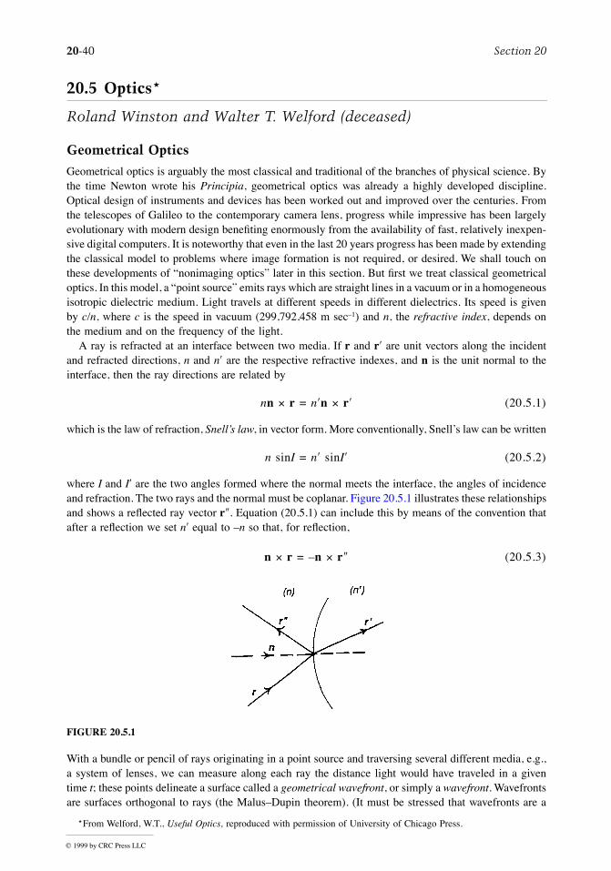
20-40 Section 20
© 1999 by CRC Press LLC
20.5 Optics*
Roland Winston and Walter T. Welford (deceased)
Geometrical Optics
Geometrical optics is arguably the most classical and traditional of the branches of physical science. Bythe time Newton wrote his Principia, geometrical optics was already a highly developed discipline.Optical design of instruments and devices has been worked out and improved over the centuries. Fromthe telescopes of Galileo to the contemporary camera lens, progress while impressive has been largelyevolutionary with modern design beneÞting enormously from the availability of fast, relatively inexpen-sive digital computers. It is noteworthy that even in the last 20 years progress has been made by extendingthe classical model to problems where image formation is not required, or desired. We shall touch onthese developments of Ònonimaging opticsÓ later in this section. But Þrst we treat classical geometricaloptics. In this model, a Òpoint sourceÓ emits rays which are straight lines in a vacuum or in a homogeneousisotropic dielectric medium. Light travels at different speeds in different dielectrics. Its speed is givenby c/n, where c is the speed in vacuum (299,792,458 m secÐ1) and n, the refractive index, depends onthe medium and on the frequency of the light.
A ray is refracted at an interface between two media. If r and r¢ are unit vectors along the incidentand refracted directions, n and n¢ are the respective refractive indexes, and n is the unit normal to theinterface, then the ray directions are related by
nn ´ r = n¢n ´ r¢ (20.5.1)
which is the law of refraction, SnellÕs law, in vector form. More conventionally, SnellÕs law can be written
n sinI = n¢ sinI¢ (20.5.2)
where I and I¢ are the two angles formed where the normal meets the interface, the angles of incidenceand refraction. The two rays and the normal must be coplanar. Figure 20.5.1 illustrates these relationshipsand shows a reßected ray vector r². Equation (20.5.1) can include this by means of the convention thatafter a reßection we set n¢ equal to Ðn so that, for reßection,
n ´ r = Ðn ´ r² (20.5.3)
With a bundle or pencil of rays originating in a point source and traversing several different media, e.g.,a system of lenses, we can measure along each ray the distance light would have traveled in a giventime t; these points delineate a surface called a geometrical wavefront, or simply a wavefront. Wavefrontsare surfaces orthogonal to rays (the MalusÐDupin theorem). (It must be stressed that wavefronts are a
FIGURE 20.5.1
*From Welford, W.T., Useful Optics, reproduced with permission of University of Chicago Press.

Patent Law and Miscellaneous Topics 20-41
© 1999 by CRC Press LLC
concept of geometrical optics and that they are not surfaces of constant phase, phase fronts, of the lightwaves in the scaler or electromagnetic wave approximations. However, in many situations the geometricalEarth are a very good approximation of phase fronts.) Thus, if successive segments of a ray are of lengthd1, d2, É, a wave front is a locus of constant Snd or, passing to the limit, òn dl. This quantity is calledan optical path length. (See Figure 20.5.2.)
Optical path lengths enter into an alternative to SnellÕs law as a basis for geometrical optics. Considerany path through a succession of media from, say, P to P¢. We can calculate the optical path length Wfrom P to P¢, and it will depend on the shape of this path, as shown in Figure 20.5.3. Then FermatÕsprinciple states that, if we have chosen a physically possible ray path, the optical path length along itwill be stationary (in the sense of the calculus of variations) with respect to small changes of the path.(The principle as originally formulated by Fermat proposed a minimum time of travel of the light.Stationarity is strictly correct, and it means roughly that, for any small transverse displacement dx of apoint on the path, the change in optical path length is of order dx2.) For our purposes, FermatÕs principleand SnellÕs law are almost equivalent, but in the case of media of continuously varying refractive indexit is sometimes necessary to invoke FermatÕs principle to establish the ray path. Apart from such cases,either one can be derived from the other.
Either Fermat or Snell can be used to develop the whole ediÞce of geometrical optics in designingoptical systems to form images.
Symmetrical Optical Systems
The axially symmetric optical system, consisting of lenses and/or mirrors with revolution symmetryarranged on a common axis of symmetry, is used to form images. Its global properties are described interms of paraxial or Gaussian optics. In this approximation only rays making small angles with the axisof symmetry and at small distances from the axis are considered. In Gaussian optics, we know fromsymmetry that rays from any point on the axis on one side of the system emerge on the other side andmeet at another point on the axis, the image point . This leads to the well-known formalism of principalplanes and focal planes shown in Figure 20.5.4. A ray entering parallel to the axis passes through F¢,the second, or image-side, principal focus on emerging from the system, and a ray entering through F,the Þrst principal focus, emerges parallel to the axis. A ray incident on the Þrst, or object-side, principalplane P at any height h emerges from the image-side principal plane P¢ at the same height h so that theprincipal planes are conjugated planes of unit magniÞcation. Excluding for the moment the special case
FIGURE 20.5.2
FIGURE 20.5.3
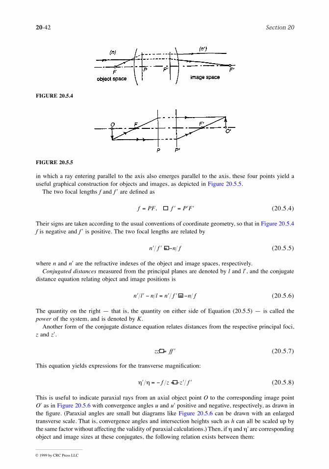
20-42 Section 20
© 1999 by CRC Press LLC
in which a ray entering parallel to the axis also emerges parallel to the axis, these four points yield auseful graphical construction for objects and images, as depicted in Figure 20.5.5.
The two focal lengths f and f ¢ are deÞned as
(20.5.4)
Their signs are taken according to the usual conventions of coordinate geometry, so that in Figure 20.5.4f is negative and f ¢ is positive. The two focal lengths are related by
(20.5.5)
where n and n¢ are the refractive indexes of the object and image spaces, respectively.Conjugated distances measured from the principal planes are denoted by l and l¢, and the conjugate
distance equation relating object and image positions is
(20.5.6)
The quantity on the right Ñ that is, the quantity on either side of Equation (20.5.5) Ñ is called thepower of the system, and is denoted by K.
Another form of the conjugate distance equation relates distances from the respective principal foci,z and z¢.
(20.5.7)
This equation yields expressions for the transverse magniÞcation:
(20.5.8)
This is useful to indicate paraxial rays from an axial object point O to the corresponding image pointO¢ as in Figure 20.5.6 with convergence angles u and u¢ positive and negative, respectively, as drawn inthe Þgure. (Paraxial angles are small but diagrams like Figure 20.5.6 can be drawn with an enlargedtransverse scale. That is, convergence angles and intersection heights such as h can all be scaled up bythe same factor without affecting the validity of paraxial calculations.) Then, if h and h¢ are correspondingobject and image sizes at these conjugates, the following relation exists between them:
FIGURE 20.5.4
FIGURE 20.5.5
f PF f P F= ¢ = ¢ ¢,
¢ ¢ = -n f n f
¢ ¢ - = ¢ ¢ = -n l n l n f n f
zz ff¢ = ¢
¢ = - = - ¢ ¢h h f z z f
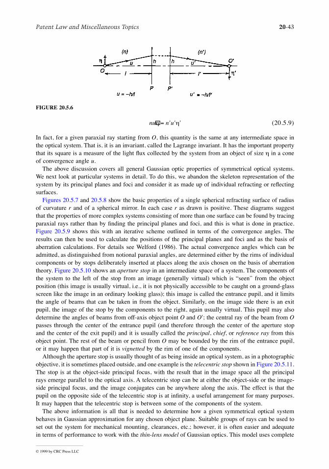
Patent Law and Miscellaneous Topics 20-43
© 1999 by CRC Press LLC
(20.5.9)
In fact, for a given paraxial ray starting from O, this quantity is the same at any intermediate space inthe optical system. That is, it is an invariant, called the Lagrange invariant. It has the important propertythat its square is a measure of the light ßux collected by the system from an object of size h in a coneof convergence angle u.
The above discussion covers all general Gaussian optic properties of symmetrical optical systems.We next look at particular systems in detail. To do this, we abandon the skeleton representation of thesystem by its principal planes and foci and consider it as made up of individual refracting or reßectingsurfaces.
Figures 20.5.7 and 20.5.8 show the basic properties of a single spherical refracting surface of radiusof curvature r and of a spherical mirror. In each case r as drawn is positive. These diagrams suggestthat the properties of more complex systems consisting of more than one surface can be found by tracingparaxial rays rather than by Þnding the principal planes and foci, and this is what is done in practice.Figure 20.5.9 shows this with an iterative scheme outlined in terms of the convergence angles. Theresults can then be used to calculate the positions of the principal planes and foci and as the basis ofaberration calculations. For details see Welford (1986). The actual convergence angles which can beadmitted, as distinguished from notional paraxial angles, are determined either by the rims of individualcomponents or by stops deliberately inserted at places along the axis chosen on the basis of aberrationtheory. Figure 20.5.10 shows an aperture stop in an intermediate space of a system. The components ofthe system to the left of the stop from an image (generally virtual) which is ÒseenÓ from the objectposition (this image is usually virtual, i.e., it is not physically accessible to be caught on a ground-glassscreen like the image in an ordinary looking glass); this image is called the entrance pupil, and it limitsthe angle of beams that can be taken in from the object. Similarly, on the image side there is an exitpupil, the image of the stop by the components to the right, again usually virtual. This pupil may alsodetermine the angles of beams from off-axis object point O and O¢; the central ray of the beam from Opasses through the center of the entrance pupil (and therefore through the center of the aperture stopand the center of the exit pupil) and it is usually called the principal, chief, or reference ray from thisobject point. The rest of the beam or pencil from O may be bounded by the rim of the entrance pupil,or it may happen that part of it is vignetted by the rim of one of the components.
Although the aperture stop is usually thought of as being inside an optical system, as in a photographicobjective, it is sometimes placed outside, and one example is the telecentric stop shown in Figure 20.5.11.The stop is at the object-side principal focus, with the result that in the image space all the principalrays emerge parallel to the optical axis. A telecentric stop can be at either the object-side or the image-side principal focus, and the image conjugates can be anywhere along the axis. The effect is that thepupil on the opposite side of the telecentric stop is at inÞnity, a useful arrangement for many purposes.It may happen that the telecentric stop is between some of the components of the system.
The above information is all that is needed to determine how a given symmetrical optical systembehaves in Gaussian approximation for any chosen object plane. Suitable groups of rays can be used toset out the system for mechanical mounting, clearances, etc.; however, it is often easier and adequatein terms of performance to work with the thin-lens model of Gaussian optics. This model uses complete
FIGURE 20.5.6
nu n uh h= ¢ ¢ ¢

20-44 Section 20
© 1999 by CRC Press LLC
FIGURE 20.5.7
FIGURE 20.5.8
FIGURE 20.5.9
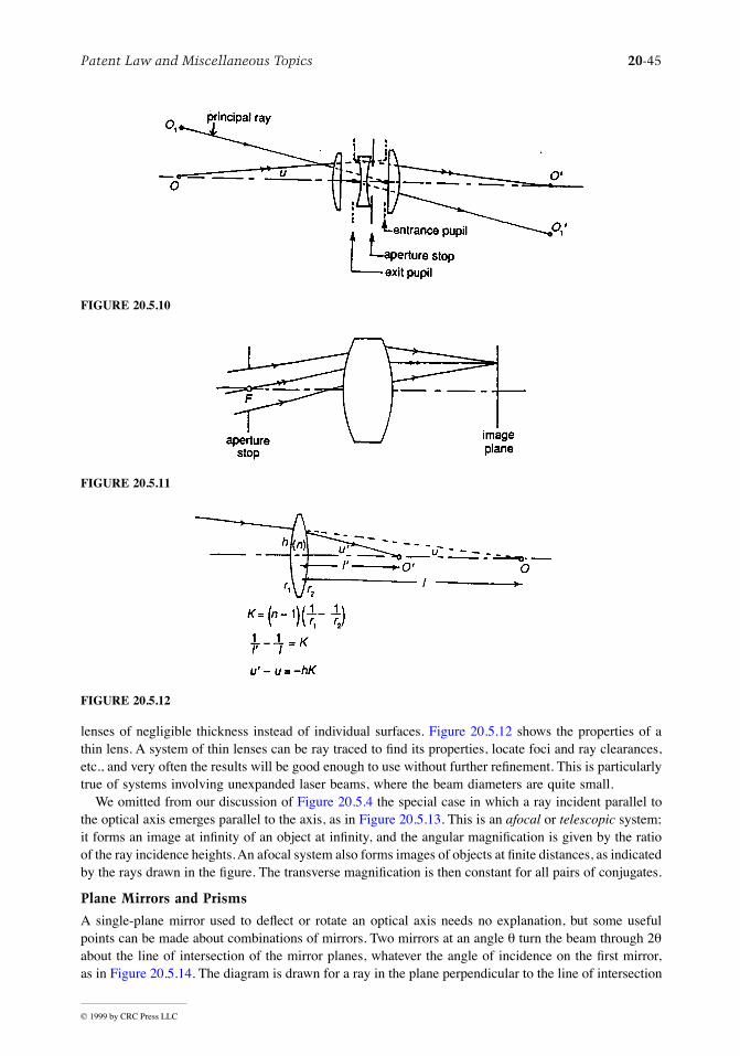
Patent Law and Miscellaneous Topics 20-45
© 1999 by CRC Press LLC
lenses of negligible thickness instead of individual surfaces. Figure 20.5.12 shows the properties of athin lens. A system of thin lenses can be ray traced to Þnd its properties, locate foci and ray clearances,etc., and very often the results will be good enough to use without further reÞnement. This is particularlytrue of systems involving unexpanded laser beams, where the beam diameters are quite small.
We omitted from our discussion of Figure 20.5.4 the special case in which a ray incident parallel tothe optical axis emerges parallel to the axis, as in Figure 20.5.13. This is an afocal or telescopic system;it forms an image at inÞnity of an object at inÞnity, and the angular magniÞcation is given by the ratioof the ray incidence heights. An afocal system also forms images of objects at Þnite distances, as indicatedby the rays drawn in the Þgure. The transverse magniÞcation is then constant for all pairs of conjugates.
Plane Mirrors and Prisms
A single-plane mirror used to deßect or rotate an optical axis needs no explanation, but some usefulpoints can be made about combinations of mirrors. Two mirrors at an angle q turn the beam through 2qabout the line of intersection of the mirror planes, whatever the angle of incidence on the Þrst mirror,as in Figure 20.5.14. The diagram is drawn for a ray in the plane perpendicular to the line of intersection
FIGURE 20.5.10
FIGURE 20.5.11
FIGURE 20.5.12
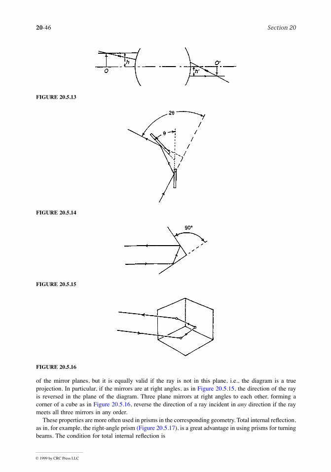
20-46 Section 20
© 1999 by CRC Press LLC
of the mirror planes, but it is equally valid if the ray is not in this plane, i.e., the diagram is a trueprojection. In particular, if the mirrors are at right angles, as in Figure 20.5.15, the direction of the rayis reversed in the plane of the diagram. Three plane mirrors at right angles to each other, forming acorner of a cube as in Figure 20.5.16, reverse the direction of a ray incident in any direction if the raymeets all three mirrors in any order.
These properties are more often used in prisms in the corresponding geometry. Total internal reßection,as in, for example, the right-angle prism (Figure 20.5.17), is a great advantage in using prisms for turningbeams. The condition for total internal reßection is
FIGURE 20.5.13
FIGURE 20.5.14
FIGURE 20.5.15
FIGURE 20.5.16
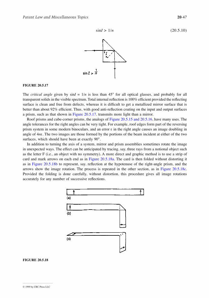
Patent Law and Miscellaneous Topics 20-47
© 1999 by CRC Press LLC
sinI > 1/n (20.5.10)
The critical angle given by sinI = 1/n is less than 45° for all optical glasses, and probably for alltransparent solids in the visible spectrum. Total internal reßection is 100% efÞcient provided the reßectingsurface is clean and free from defects, whereas it is difÞcult to get a metallized mirror surface that isbetter than about 92% efÞcient. Thus, with good anti-reßection coating on the input and output surfacesa prism, such as that shown in Figure 20.5.17, transmits more light than a mirror.
Roof prisms and cube-corner prisms, the analogs of Figure 20.5.15 and 20.5.16, have many uses. Theangle tolerances for the right angles can be very tight. For example, roof edges form part of the reversingprism system in some modern binoculars, and an error e in the right angle causes an image doubling inangle of 4ne. The two images are those formed by the portions of the beam incident at either of the twosurfaces, which should have been at exactly 90°.
In addition to turning the axis of a system, mirror and prism assemblies sometimes rotate the imagein unexpected ways. The effect can be anticipated by tracing, say, three rays from a notional object suchas the letter F (i.e., an object with no symmetry). A more direct and graphic method is to use a strip ofcard and mark arrows on each end as in Figure 20.5.18a. The card is then folded without distorting itas in Figure 20.5.18b to represent, say, reßection at the hypotenuse of the right-angle prism, and thearrows show the image rotation. The process is repeated in the other section, as in Figure 20.5.18c.Provided the folding is done carefully, without distortion, this procedure gives all image rotationsaccurately for any number of successive reßections.
FIGURE 20.5.17
FIGURE 20.5.18
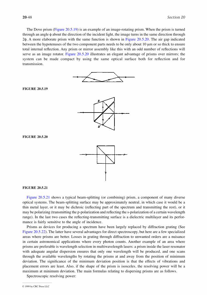
20-48 Section 20
© 1999 by CRC Press LLC
The Dove prism (Figure 20.5.19) is an example of an image-rotating prism. When the prism is turnedthrough an angle f about the direction of the incident light, the image turns in the same direction through2f. A more elaborate prism with the same function is shown in Figure 20.5.20. The air gap indicatedbetween the hypotenuses of the two component parts needs to be only about 10 mm or so thick to ensuretotal internal reßection. Any prism or mirror assembly like this with an odd number of reßections willserve as an image rotator. Figure 20.5.20 illustrates an elegant advantage of prisms over mirrors; thesystem can be made compact by using the same optical surface both for reßection and fortransmission.
Figure 20.5.21 shows a typical beam-splitting (or combining) prism, a component of many diverseoptical systems. The beam-splitting surface may be approximately neutral, in which case it would be athin metal layer, or it may be dichroic (reßecting part of the spectrum and transmitting the rest), or itmay be polarizing (transmitting the p-polarization and reßecting the s-polarization of a certain wavelengthrange). In the last two cases the reßecting-transmitting surface is a dielectric multilayer and its perfor-mance is fairly sensitive to the angle of incidence.
Prisms as devices for producing a spectrum have been largely replaced by diffraction grating (SeeFigure 20.5.22). The latter have several advantages for direct spectroscopy, but here are a few specializedareas where prisms are better. Losses in grating through diffraction to unwanted orders are a nuisancein certain astronomical applications where every photon counts. Another example of an area whereprisms are preferable is wavelength selection in multiwavelength lasers: a prism inside the laser resonatorwith adequate angular dispersion ensures that only one wavelength will be produced, and one scansthrough the available wavelengths by rotating the prisms at and away from the position of minimumdeviation. The signiÞcance of the minimum deviation position is that the effects of vibrations andplacement errors are least. Also, if the shape of the prism is isosceles, the resolving power will be amaximum at minimum deviation. The main formulas relating to dispersing prisms are as follows.
Spectroscopic resolving power:
FIGURE 20.5.19
FIGURE 20.5.20
FIGURE 20.5.21
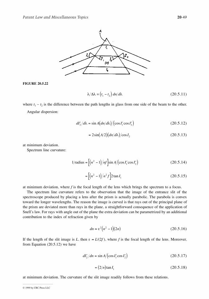
Patent Law and Miscellaneous Topics 20-49
© 1999 by CRC Press LLC
(20.5.11)
where t1 Ð t2 is the difference between the path lengths in glass from one side of the beam to the other.
Angular dispersion:
(20.5.12)
(20.5.13)
at minimum deviation.Spectrum line curvature:
(20.5.14)
(20.5.15)
at minimum deviation, where f is the focal length of the lens which brings the spectrum to a focus.The spectrum line curvature refers to the observation that the image of the entrance slit of the
spectroscope produced by placing a lens after the prism is actually parabolic. The parabola is convextoward the longer wavelengths. The reason the image is curved is that rays out of the principal plane ofthe prism are deviated more than rays in the plane, a straightforward consequence of the application ofSnellÕs law. For rays with angle out of the plane the extra deviation can be parametrized by an additionalcontribution to the index of refraction given by
(20.5.16)
If the length of the slit image is L, then e » L/(2f ), where f is the focal length of the lens. Moreover,from Equation (20.5.12) we have
(20.5.17)
(20.5.18)
at minimum deviation. The curvature of the slit image readily follows from these relations.
FIGURE 20.5.22
l l lD = t t dn d1 2-( )
dI d A dn d I I¢ = ( ) ¢ ¢( )2 1 2l lsin cos cos
= ( )( )2 2 2sin cosA dn d Il
1 121 2radius = -( )[ ] ¢ ¢( )n nf A I Isin cos cos
= -( )[ ]n n f I2 211 2 tan
dn n n» -( )( )e2 2 1 2
dI dn A I I¢ = ¢ ¢( )2 1 2sin cos cos
= ( )2 1n Itan

20-50 Section 20
© 1999 by CRC Press LLC
The typical dispersing prism of constant deviation shown in Figure 20.5.23 has the property that, ifit is placed in a collimated beam, the wavelength which emerges at right angles to the incident beam isalways at minimum deviation so that the spectrum is scanned by rotating the prism about a suitable axissuch as the one indicated.
A prism used a long way from minimum deviation will expand or contract a collimated beam in onedimension. Figure 20.5.24 shows a pair of prisms used in this way to turn a laser beam of ellipticalproÞle (from a diode laser) into a beam of circular proÞle by expanding it in the plane of the diagram only.
Nonimaging Optics
In one important respect conventional image-forming optical design is quite inefÞcient, that is, in merelyconcentrating and collecting light. This is well illustrated by an example taken from solar energyconcentration (Figure 20.5.25). The ßux at the surface of the sun (»63 W/mm2) falls off inversely withthe square of the distance to a value »1.37 mW/mm2 above the Earth's atmosphere or typically 0.8 to 1mW/mm2 on the ground. The second law of thermodynamics permits an optical device (in principle) toconcentrate the dilute solar ßux at Earth so as to attain temperatures up to but not exceeding that of thesun's surface. This places an upper limit on the solar ßux density achievable on Earth and correspondinglyon the concentration ratio of any optical device. From simple geometry, this limiting concentration ratiois related to the sun's angular size (2q) by Cmax = 1/sin2q » 1/q2 (small angle approximation). We willcall this thermodynamic limit the sine law of concentration. Therefore, since q = 0.27° or 4.67 mrad,Cmax » 46,000. When the target is immersed in a medium of refractive index n, this limit is increasedby a factor n2, Cmax = n2/sin2q. This means that a concentration of about 100,000 will be the upper limitfor ordinary (n » 1.5) refractive materials. In experiments at the University of Chicago we actuallyachieved a solar concentration of 84,000 by using a nonimaging design with a refractive medium(sapphire). We would not even have come close using conventional designs, not for any fundamentalreason but because imaging optical design is quite inefÞcient for delivering maximum concentration.For example, consider the paraboloidal mirror of a telescope used to concentrate sunlight at its focus(Figure 20.5.26). We can relate the concentration ratio to the angle 2f subtended by the paraboloid at
FIGURE 20.5.23
FIGURE 20.5.24
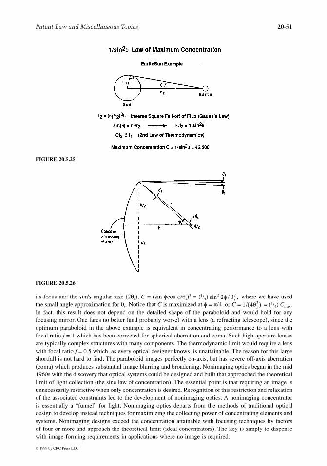
Patent Law and Miscellaneous Topics 20-51
© 1999 by CRC Press LLC
its focus and the sun's angular size (2qs), C = (sin fcos f/qs)2 = (1/4) where we have usedthe small angle approximation for qs. Notice that C is maximized at f = p/4, or C = = (1/4) Cmax.In fact, this result does not depend on the detailed shape of the paraboloid and would hold for anyfocusing mirror. One fares no better (and probably worse) with a lens (a refracting telescope), since theoptimum paraboloid in the above example is equivalent in concentrating performance to a lens withfocal ratio f = 1 which has been corrected for spherical aberration and coma. Such high-aperture lensesare typically complex structures with many components. The thermodynamic limit would require a lenswith focal ratio f = 0.5 which, as every optical designer knows, is unattainable. The reason for this largeshortfall is not hard to Þnd. The paraboloid images perfectly on-axis, but has severe off-axis aberration(coma) which produces substantial image blurring and broadening. Nonimaging optics began in the mid1960s with the discovery that optical systems could be designed and built that approached the theoreticallimit of light collection (the sine law of concentration). The essential point is that requiring an image isunnecessarily restrictive when only concentration is desired. Recognition of this restriction and relaxationof the associated constraints led to the development of nonimaging optics. A nonimaging concentratoris essentially a ÒfunnelÓ for light. Nonimaging optics departs from the methods of traditional opticaldesign to develop instead techniques for maximizing the collecting power of concentrating elements andsystems. Nonimaging designs exceed the concentration attainable with focusing techniques by factorsof four or more and approach the theoretical limit (ideal concentrators). The key is simply to dispensewith image-forming requirements in applications where no image is required.
FIGURE 20.5.25
FIGURE 20.5.26
sin / ,2 22f qs
1 4 2/( )qs

20-52 Section 20
© 1999 by CRC Press LLC
Since its inception, the Þeld has undergone three periods of rapid conceptual development. In the1970s the ÒstringÓ (see Figures 20.5.27 and 20.5.28) or Òedge-rayÓ method (see Welford and Winston,1989) was formulated and elaborated for a large variety of geometries. This development was driven bythe desire to design wide-angle solar concentrators. It may be succinctly characterized as òn dl = constantalong a string. (Notice that replacing ÒstringÓ by Òray,Ó Fermat's principle, gives all of imaging optics.)In the early 1980s, a second class of algorithms was found, driven by the desire to obtain ideally perfectsolutions in three dimensions (3D) (The ÒstringÓ solutions are ideal only in 2D, and as Þgures ofrevolution in 3D are only approximately ideal, though still very useful.) This places reßectors along thelines of ßow of a radiation Þeld set up by a radiating lambertian source. In cases of high symmetry suchas a sphere or disk, one obtains ideal solutions in both 2D and 3D. The third period of rapid developmenthas taken place only in the past several years; its implications and consequences are still in the processof being worked out. This was driven by the desire to address a wider class of problems in illuminationthat could not be solved by the old methods, for example, uniformly illuminating a plane (e.g., a tableor a wall) by a lambertian light source (e.g., a ßuorescent light). It is well known that the far-Þeldilluminance from a lambertian source falls off with a power of the cosine of the radiating angle q. Forexample, cylindrical radiators (such as a ßuorescent lamp) produce a cos2q illuminance on a distantplane, strip radiators produce a cos3q illuminance, while circular disk radiators produce a cos4q illumi-nance. But suppose one desires a predetermined far-Þeld illuminance pattern, e.g., uniform illuminance?The old designs will not sufÞce; they simply transform a lambertian source radiating over 2p into alambertian source radiating over a restricted set of angles. The limitation of the old designs is that theyare too static and depend on a few parameters, such as the area of the beam A1 and the divergence angleq. One needs to introduce additional degrees of freedom into the nonimaging designs to solve a widerclass of problems.
Edge-Ray Optics
One way to design nonimaging concentrators is to reßect the extreme input rays into the extreme outputrays. We call this the Òedge-ray method.Ó An intuitive realization of this method is to wrap a string aboutboth the light source and the light receiver, then allow the string to unwrap from the source and wraparound the receiver. In introducing the string picture, we follow an insight of Hoyt Hottel (MassachusettsInstitute of Technology), who discovered many years ago that the use of strings tremendously simpliÞedthe calculation of radiative energy transfer between surfaces in a furnace. Our string is actually a ÒsmartÓ
FIGURE 20.5.27

Patent Law and Miscellaneous Topics 20-53
© 1999 by CRC Press LLC
string; it measures the optical path length (ordinary length times the index of refraction) and refracts inaccordance with Snell's law at the interface between different refracting materials. òn dl = constant. Thelocus traced out turns out to be the correct reßecting surface! LetÕs see how this works in the simplestkind of problem nonimaging optics addresses: collecting light over an entrance aperture AA¢ with angulardivergence ±q and concentrating the light onto an exit aperture BB¢ (Figure 20.5.27). We attach one endof the string to the edge of the exit aperture B and the loop at the other end over a line WW¢ inclinedat angle q to the entrance aperture (this is the same as attaching to a Òpoint at inÞnityÓ). We now unwrapthe string and trace out the locus of the reßector taking care that string is taut and perpendicular to WW¢.Then we trace the locus of the other side of the reßector. We can see with a little algebra that when weare done the condition for maximum concentration has been met. When we start unwrapping the string,the length is AB¢ + BB¢; when we Þnish, the same length is WA¢ + A¢B. But WA¢ = AA¢sinq, while AB¢= A¢B. So we have achieved AA¢/BB¢ = 1/sinq which is maximum concentration! To see why this works,we notice that the reßector directs all rays at ±q to the edges BB¢ so that rays at angles > ±q are reßectedout of the system and rejected. Now there is a conservation theorem for light rays called conservationof phase space or ÒetendueÓ which implies that if the rays at angles > ±q are rejected, then the rays thathave angles <q are all collected. Next we can try a more-challenging problem, where the Òexit apertureÓis a cylinder of radius a (Figure 20.5.28). Now we attach the string to a point on the cylinder and wrapit around the cylinder. When the string is unwrapped, we Þnd that AA¢/2pa = 1/sinq which is maximumconcentration on the surface of the cylinder! Such designs are useful for solar-thermal concentratorssince the typical receiver is a tube for carrying ßuid. A solar plant for powering air conditioners thatuses this design is shown in Figure 20.5.29. As already mentioned, there is an alternative method fordesigning ÒidealÓ optical systems which bears little resemblance to the Òstring methodÓ already described.We picture the aggregate of light rays traversing an optical system as a ßuid ßow in an abstract spacecalled phase space.This is the ÒspaceÓ of ray positions and ray directions multiplied by the index ofrefraction, so it has twice the number of dimensions of ordinary space. By placing reßectors along thelines of ßow of this vector Þeld, nonimaging designs are generated. Flow-line designs are perfect inthree dimensions, while the string designs rotated about an axis are not. On the other hand, the numberof ßow-line designs are much more restricted. For details see Welford and Winston (1989).
FIGURE 20.5.28

20-54 Section 20
© 1999 by CRC Press LLC
Lasers
Lasers are by now a ubiquitous light source with certain properties in addition to coherence andmonochromaticity which have to be taken account of in some applications. Aside from many researchapplications of lasers, the HeNe laser at 632.8 nm wavelength has been available for several decadesfor alignment, surveying, and the like. But the explosive uses of lasers have come only recently withthe advent of the solid-state diode laser. To appreciate the convenience of diode lasers one can drawupon the analogy between transistors and vacuum tubes. Inexpensive diode lasers are in widespread usein compact disk players, optical disk readers, and Þber-optics communications. The list of consumerapplications is growing rapidly (e.g., laser pointers). In addition, diode lasers are used in arrays tooptically drive (pump) more powerful lasers. The radiation that lasers emit can be highly coherent, and,except for the wavelength, of the same general character as the radiation from a radio frequency oscillator.We can identify four elements common to nearly all lasers (we follow the discussion in Mandel andWolf, 1995, which should be consulted for details):
1. An optical resonator, generally formed by two or more mirrors;2. A gain medium in which an inverted atomic population between the laser energy levels is
established;3. An optical pump or energy source to excite the gain medium;4. A loss mechanism by which energy is dissipated or dispersed.
Figure 20.5.30 shows a typical form of laser, in which the resonator is a FabryÐPerot interferometer,and the ampliÞer is a gas plasma tube wherein a discharge is maintained. To reduce reßection lossesfrom the plasma tube, its end windows are generally arranged at the Brewster angle for linearly polarizedlight at the laser frequency. The end mirrors are usually provided with multilayer dielectric coatings tomake them highly reßecting. Of course, the output mirror needs to have its reßectivity, R, less than
FIGURE 20.5.29

Patent Law and Miscellaneous Topics 20-55
© 1999 by CRC Press LLC
100%, so that (1 Ð R) is commonly the main source of the energy loss that has to be compensated bythe gain medium. The cavity mirrors play the important role of feeding photons belonging to the lasermodes back into the laser cavity. Most of the spontaneously emitted photons traveling in various otherdirections are lost. However, photons associated with a cavity resonance mode interact repeatedly withthe atoms of the gain medium, and their number grows through stimulated emission, as illustrated inFigure 20.5.31. Once one mode is sufÞciently populated, the probability for stimulated emission intothat mode exceeds the spontaneous emission probability. In general, when the rate at which photons arefed into the optical cavity mode exceeds the rate at which they are lost from the cavity by the lossmechanism, the amplitude of the laser Þeld starts to grow until a steady state is reached. At that pointthe rate of radiation by the laser equals the net rate at which energy is supplied. It is easy to see thatthis is achievable by an inverted population between the two atomic laser levels, with more atoms inthe upper laser state than in the lower. If N2, N1 are the upper state and lower state populations, the rateof absorption of laser photons by the atomic system is proportional to N1, and the rate of stimulatedemission of laser photons by the system is proportional to N2, with the same constant of proportionalityfor both. If N2 exceeds N1 sufÞciently, all the radiation losses can be made good by the atomic system.It can be shown that the condition for laser action (in a single mode) is
(20.5.19)
where A is the cross-sectional area of the laser and l is the wavelength.We next summarize how the special properties of laser beams are to be taken into account in optical
design. The well-known Gaussian intensity proÞle of laser beams persists if it is taken through a sequenceof lenses along the axis, and at certain points that can be more-or-less predicted by paraxial optics aÒfocusÓ is formed. But when, as often happens, the convergence angle in the space in which this occursis small, say, 1 mrad or less, some departures from the predictions of the paraxial optics occur. We shallexamine these effects, since they are of importance in many of the systems already mentioned.
Gaussian Beams
In paraxial approximation the simplest form of a single-mode beam is the TEM00 Gaussian beam shownin Figure 20.5.32. Starting from the narrowest part, known as the waist, the beam diverges with sphericalphase fronts. The complex amplitude at the waist has the form
(20.5.20)
where w0 is called the beam width and r is a radial coordinate.
FIGURE 20.5.30 A simple form of laser.
FIGURE 20.5.31 Illustration of the growth of the stimulated emission probability with the intensity of the mode.
N N A R2 122 1- > -( ) l
A A r= -( )02
02exp w

20-56 Section 20
© 1999 by CRC Press LLC
At a distance z along the beam in either direction, the complex amplitude is, apart from a phase factor,
(20.5.21)
where w is given by
(20.5.22)
At a distance z from the waist, the phase fronts have a radius of curvature R given by
(20.5.23)
The beam contour of constant intensity is a hyperboloidal surface of (small) asymptotic anglegiven by
(20.5.24)
It can be seen that the centers of curvature of the phase fronts are not at the beam waist; in fact thephase front is plane at that point. The geometrical wavefronts are not exactly the same as true phasefronts, and if in this case we postulate that geometrical wavefronts should have their centers of curvatureat the beam waist, we have an example of this. However, the difference is small unless the convergenceangle is very small or, more precisely, when the Fresnel number of the beam is not much larger than unity:
(20.5.25)
There is nothing special about Gaussian beams to cause this discrepancy between phase fronts andgeometrical wavefronts; a similar phenomenon occurs with beams which are sharply truncated by thepupil (Òhard-edgedÓ beams). But it happens that it is less usual to be concerned with the region near thefocus of a hard-edged beam of small Fresnel number, whereas Gaussian beams are frequently used inthis way. Thus, Born and Wolf, Principles of Optics (1959) show that the phase front at the focus of ahard-edged beam is also plane, but with rapid changes of intensity and phase jumps across the zeros ofintensity.
Tracing Gaussian Beams
If the beam is in a space of large convergence angle, say, greater than 10 mrad, it can be traced byordinary paraxial optics, i.e., using the assumption that for all practical purposes the phase fronts arethe same as geometrical wavefronts. In a space of small convergence angle it is necessary to propagatethe beam between refracting surfaces by means of the proper Gaussian beam formulas and then useparaxial optics to refract (or reßect) the phase front through each surface in turn. To do this, we need
FIGURE 20.5.32
A A r= ( ) -( )w w w0 02
02exp
w w l pwz z( ) = + ( )[ ]0 02
1 21
R z z z( ) = + ( )[ ]1 02 2
pw l
A e02 2/
q l pw= 0
Fresnel number = 2w lR

Patent Law and Miscellaneous Topics 20-57
© 1999 by CRC Press LLC
two more formulas to give the position, z, and size of the beam waist starting from the beam size andphase front curvature at an arbitrary position on the axis, i.e., given w and R. These are
(20.5.26)
and
(20.5.27)
Equations (20.5.22) to (20.5.27) enable a Gaussian beam to be traced through a sequence of refractingsurfaces as an iterative process. Thus, starting from a beam waist of given size w0 (and angle given byEquation (20.5.24)), we move a distance z to the Þrst refracting surface. At this surface the beam sizew is given by Equation (20.5.22) and the radius of curvature R of the phase front is given by Equation(20.5.23). The radius of curvature R¢ of the refracted phase front is obtained by paraxial optics usingthe equation of Figure 20.5.7 and taking R and R¢ as the conjugate distances l and l¢. Then the positionand size of the new beam waist are found from Equations (20.5.26) and (20.5.27). These procedurescan be carried through all the refracting surfaces of the optical system.
It can be seen from Equation (20.5.26) that z and R are substantially equal when lR/pw2 is very small.When this is so, there is no need to use these special equations for transferring between surfaces; theiterative equations in Figure 20.5.9 can be used, with the understanding that the paraxial convergenceangle u is the equivalent of the asymptotic angle q in Equation (20.5.24).
There are no simple equations for hard-edged beams corresponding to Equations (20.5.23) to (20.5.27)for use with very small convergence angles. Numerical calculations of the beam patterns near focus havebeen published for some special cases, and these show, as might be expected, very complex structuresnear the ÒfocalÓ region; however, that is deÞned.
Truncation of Gaussian Beams
The theoretical origin of the Gaussian beam is as a paraxial solution of the Helmholtz equation, i.e., asolution concentrated near one straight line, the axis, but although most of the power is within the regionnear the axis the solution is nonzero, although very small, at an inÞnite distance from the axis. Thus,the Gaussian proÞle is truncated when it passes through any aperture of Þnite diameter Ñ e.g., a lensmount, an aperture stop, or even the Þnite-diameter end mirror of a laser resonator Ñ after which it isno longer Gaussian and the above equations are no longer valid! In practice, this need not be a problem,for if the radius of the aperture is 2w, the complex amplitude is down to 1.8% of its value at the centerand the intensity is 0.03% of its value at the center. Thus, it is often assumed that an aperture of radius2w has no signiÞcant effect on the Gaussian beam, and this assumption is adequate for many purposes,although not all.
Sometimes it is useful to truncate a Gaussian beam deliberately, i.e., turn it into a hard-edged beam,by using an aperture of radius less than, say, w. In this way an approximation to the Airy pattern isproduced at the focus instead of a Gaussian proÞle waist, and this pattern may be better for certainpurposes, e.g., for printers where the spot must be as small as possible for an optical system of givennumerical aperture.
Gaussian Beams and Aberrations
In principle, a Gaussian beam is a paraxial beam, from the nature of the approximations made in solvingthe Helmholtz equation. However, Gaussian beams can be expanded to large diameters simply by lettingthem propagate a large distance, and they can acquire aberrations by passing through an aberrating lensor mirror system. The beam is then no longer Gaussian, of course, in the strict sense, but we stress thatthe conventional optical design idea involving balancing and reduction of aberrations can be applied to
z R z= + ( )[ ]-1 2
1l pw
w w pw l02 2 1 2
1= + ( )[ ]-
R
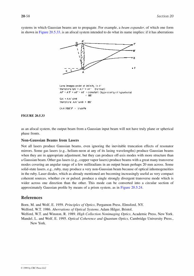
20-58 Section 20
© 1999 by CRC Press LLC
systems in which Gaussian beams are to propagate. For example, a beam expander, of which one formin shown in Figure 20.5.33, is an afocal system intended to do what its name implies: if it has aberrations
as an afocal system, the output beam from a Gaussian input beam will not have truly plane or sphericalphase fronts.
Non-Gaussian Beams from Lasers
Not all lasers produce Gaussian beams, even ignoring the inevitable truncation effects of resonatormirrors. Some gas lasers (e.g., helium-neon at any of its lasing wavelengths) produce Gaussian beamswhen they are in appropriate adjustment, but they can produce off-axis modes with more structure thana Gaussian beam. Other gas lasers (e.g., copper vapor lasers) produce beams with a great many transversemodes covering an angular range of a few milliradians in an output beam perhaps 20 mm across. Somesolid-state lasers, e.g., ruby, may produce a very non-Gaussian beam because of optical inhomogeneitiesin the ruby. Laser diodes, which as already mentioned are becoming increasingly useful as very compactcoherent sources, whether cw or pulsed, produce a single strongly divergent transverse mode which iswider across one direction than the other. This mode can be converted into a circular section ofapproximately Gaussian proÞle by means of a prism system, as in Figure 20.5.24.
References
Born, M. and Wolf, E. 1959. Principles of Optics, Pergamon Press, Elmsford, NY.Welford, W.T. 1986. Aberrations of Optical Systems, Adam Hilger, Bristol.Welford, W.T. and Winston, R. 1989. High Collection Nonimaging Optics, Academic Press, New York.Mandel, L. and Wolf, E. 1995. Optical Coherence and Quantum Optics, Cambridge University Press.,
New York.
FIGURE 20.5.33

Patent Law and Miscellaneous Topics 20-59
© 1999 by CRC Press LLC
20.6 Water Desalination
Noam Lior
Introduction and Overview
Water desalination is a process that separates water from a saline water solution. The natural water cycleis the best and most prevalent example of water desalination. Ocean waters evaporate due to solar heatingand atmospheric inßuences; the vapor consisting mostly of fresh water (because of the negligible volatilityof the salts at these temperatures) rises buoyantly and condenses into clouds in the cooler atmosphericregions, is transported across the sky by cloud motion, and is eventually deposited back on the earthsurface as fresh water rain, snow, and hail. The global freshwater supply from this natural cycle is ample,but many regions on Earth do not receive an adequate share. Population growth, rapidly increasingdemand for fresh water, and increasing contamination of the available natural fresh water resourcesrender water desalination increasingly attractive. Water desalinaiton has grown over the last four decadesto an output of about 20 million m3 of fresh water per day, by about 10,000 sizeable land-based waterdesalination plants.
The salt concentration in the waters being desalted ranges from below 100 ppm wt. (essentially freshwater, when ultrapure water is needed), through several thousand parts per million (brackish watersunsuitable for drinking or agricultural use) and seawater with concentrations between 35,000 and 50,000ppm. OfÞcial salt concentration limits for drinkable water are about 1000 ppm, and characteristic watersupplies are restricted to well below 500 ppm, with city water in the United States being typically below100 ppm. Salinity limits for agricultural irrigation waters depend on the type of plant, cultivation, andsoil, but are typically below 2000 ppm.
Many ways are availiable for separating water from a saline water solution. The oldest and stillprevalent desalination process is distillation. The evaporation of the solution is effected by the additionof heat or by lowering of its vapor pressure, and condensation of these vapors on a cold surface producesfresh water. The three dominant distillation processes are multistage ßash (MSF), multieffect (ME), andvapor compression (VC). Until the early 1980s the MSF process was prevalent for desalination. Nowmembrane processes, especially reverse osmosis (RO), are economical enough to have taken about onethird of the market. In all membrane processes separation occurs due to the selective nature of thepermeability of a membrane, which permits, under the inßuence of an external driving force, the passageof either water or salt ions but not of both. The driving force may be pressure (as in RO), electric potential(as in electrodialysis, ED), or heat (as in membrane distillation, MD). A process used for low-salinitysolutions is the well-known ion exchange (IE), in which salt ions are preferentially adsorbed onto amaterial that has the required selective adsorption property and thus reduce the salinity of the water inthe solution.
The cost of desalted water is comprised of the capital cost of the plant, the cost of the energy neededfor the process, and the cost of operation and maintenance staff and supplies. In large seawater desali-nation plants the cost of water is about $1.4 to $2/m3, dropping to less than $1/m3 for desalting brackishwater. A methodology for assessing the economic viability of desalination in comparison with otherwater supply methods is described by Kasper and Lior (1979). Desalination plants are relatively simpleto operate, and progress toward advanced controls and automation is gradually reducing operationexpenses. The relative effect of the cost of the energy on the cost of the fresh water produced dependson local conditions, and is up to one half of the total.
The boiling point of a salt solution is elevated as the concentration is increased, and the boiling pointelevation is a measure of the energy needed for separation. Thermodynamically reversible separationdeÞnes the minimal energy requirement for that process. The minimal energy of separation Wmin in sucha process is the change in the Gibbs free energy between the beginning and end of the process, DG. Theminimal work when the number of moles of the solution changes from n1 to n2 is thus
20-60 Section 20
© 1999 by CRC Press LLC
(20.6.1)
The minimal energy of separation of water from seawater containing 3.45 wt.% salt, at 25°C, is 2.55kJ/(kg fresh water) for the case of zero fresh water recovery (inÞnitesimal concentration change) and2.91 kJ/(kg fresh water) for the case of 25% freshwater recovery. Wmin is, however, severalfold smallerthan the energy necessary for water desalination in practice. Improved energy economy can be obtainedwhen desalination plants are integrated with power generation plants (Aschner, 1980). Such dual-purposeplants save energy but also increase the capital cost and complexity of operation.
Two aspects of the basically simple desalination process require special attention. One is the high-corrosivity of seawater, especially pronounced in the higher-temperature destillation processes, whichrequires the use of corrosion-resistant expensive materials. Typical materials in use are copperÐnickelalloys, stainless steel, titanium, and, at lower temperatures, Þber-reinforced polymers (George et al.,1975). Another aspect is scale formation (Glater et al., 1980; Heitman, 1990). Salts in saline water,particularly calcium sulfate, magnesium hydroxide, and calcium carbonate, tend to precipitate when acertain temperature and concentration are exceeded. The precipitate, often mixed with dirt entering withthe seawater and with corrosion products, will gradually plug up pipes, and when depositing on heattransfer surfaces reduces heat transfer rates and thus impairs plant performance. While the ambient-temperature operation of membrane processes reduces scaling, membranes are much more susceptiblenot only to minute amounts of scaling or even dirt, but also to the presence of certain salts and othercompounds that reduce their ability to separate salt from water. To reduce corrosion, scaling, and otherproblems, the water to be desalted is pretreated. The pretreatment consists of Þltration, and may inluderemoval of air (deaeration), removal of CO2 (decarbonation), and selective removal of scale-formingsalts (softening). It also includes the addition of chemicals that allow operation at higher temperatureswithout scale deposition, or which retard scale deposition and/or cause the precipitation of scale whichdoes not adhere to solid surfaces, and that prevent foam formation during the desalination process.
Saline waters, including seawater, contain, besides a variety of inorganic salts, also organic materialsand various particles. They differ in composition from site to site, and also change with time due to bothnatural and person-made causes. Design and operation of desalination plants requires good knowledgeof the saline water composition and properties (Fabuss, 1980; Heitman, 1991).
The major water desalination processes that are currently in use or in advanced research stages areconcisely described below. Information on detailed modeling can be found in the references.
Distillation Processes
Multistage Flash Evaporation (MSF)
Almost all of the large desalination plants use the MSF process shown schematically in Figure 20.6.1.A photo of an operating plant is shown in Figure 20.6.2. The seawater feed is preheated by internal heatrecovery from condensing water vapor during passage through a series of stages, and then heated to itstop temperature by steam generated by an external heat source. The hot seawater then ßows as a horizontalfree-surface stream through a series of Òstages,Ó created by vertical walls which separate the vapor spaceof each stage from the others. These walls allow the vapor space of each stage to be maintained at adifferent pressure, which is gradually decreased along the ßow path due to the gradually decreasingtemperature in the condenser/seawater-preheater installed above the free stream. The seawater is super-heated by a few degrees celsius relative to the vapor pressure in each stage it enters, and consequentlyevaporates in each stage along its ßow path. The latent heat of the evaporation is supplied by equivalentreduction of the sensible heat of the evaporating water, thus resulting in a gradual lowering of the streamtemperature. The evaporation is vigorous, resulting in intensive bubble generation and growth withaccompanying stream turbulence, a process known as ßash evaporation (Lior and Greif, 1980; Miyatakeet al., 1992; 1993). One of the primary advantages of the MSF process is the fact that evaporation occurs
W G dnn
n
Wmin = ( )ò1
2
D

Paten
t Law
and
Miscellan
eous Topics
20-61
© 1999 by CRC Press LLC
FIGURE 20.6.1 Schematic ßow and temperature diagram of the MSF process, for a recirculation type plant.

20-62 Section 20
© 1999 by CRC Press LLC
from the saline water stream and not on heated surfaces (as in other distillation processes such assubmerged tube and ME evaporation) where evaporation typically causes scale depostition and thusgradual impairment of heat transfer rates. Also, the fact that the sensible heat of water is much smallerthan its latent heat of evaporation, where the speciÞc heat cp = 4.182 kJ/kg/°C change of water temperatureand the latent heat is hfg = 2378 kJ/kg, and the fact that the top temperature is limited by considerationsof scaling and corrosion, dictate the requirement for a very large ßow rate of the evaporating stream.For example (in the following, the subscripts b, d, and s refer to brine distillate, and steam, respectively),operating between a typical top temperature Tb,t of 90°C at the inlet to the evaporator and an exittemperature Tb,e of 40°C corresponding to the ambient conditions, the overall temperature drop of theevaporating stream if 50°C. By using these values, the heat balance between the sensible heat of thewater stream, ßowing at a mass ßow rate and the latent heat needed for generating water vapor(distillate) at a mass ßow rate is
(20.6.2)
which yields the brine-to-product mass ßow ratio as
(20.6.3)
Therefore, 12.37 kg of saline water are needed to produce 1 kg of distillate. This high ßow rate incurscorresponding pumping equipment and energy expenses, sluggish system dynamics, and, since the streamlevel depth is limited to about 0.3 to 0.5 m for best evaporation rates, also requires large evaporatorvessels with their associated expense.
The generated water vapor rises through a screen (ÒdemisterÓ) placed to remove entrained saline waterdroplets. Rising further, it then condenses on the condenser tube bank, and internal heat recovery is
FIGURE 20.6.2 One of the six units of the 346,000 m3/day MSF desalination plant Al Taweelah B in Abu Dhabi,United Arab Emirates. (Courtesy of Italimpianti S. p. A.) It is a dual-purpose plant, composed of six identical powerand desalination units. Five of the six boilers are seen in the background. The desalination units were in 1996 thelargest in the world. They have 17 recovery and 3 reject stages and a performance ratio (PR) of 8.1. The plant alsoproduces 732 MWe of power.
Ç ,mb
Çmd
Ç Ç Ç, ,m m c T T m hb d p b t b e d fg-( ) -( ) »
Ç
Ç ..
, ,
m
m
h
c T Tb
d
fg
p b t b e
=-( )
+ =( )( )
+ =12378
4 182 501 12 37
Patent Law and Miscellaneous Topics 20-63
© 1999 by CRC Press LLC
achieved by transferring its heat of condensation to the seawater feed that is thus being preheated. Thisinternal heat recovery is another of the primary advantages of the MSF process. The energy performanceof distillation plants is often evaluated by the performance ratio, PR, typically deÞned as
(20.6.4)
where is the mass ßow rate of heating steam. Since the latent heat of evaporation is almost the samefor the distillate and the heating steam, PR is also the ratio of the heat energy needed for producing oneunit mass of product (distillate) to the external heat actually used for that purpose. Most of the heatingof the brine stream to the top temperature Tb,t is by internal heat recovery, and as seen in Figure 20.6.1,the external heat input is only the amount of heat needed to elevate the temperature of the preheatedbrine from its exit from the hottest stage at Tb,2 to Tb,t. Following the notation in Figure 20.6.1, and usingheat balances similar to that in Equation (20.6.3) for the brine heater and ßash evaporator, the PR canthus also be deÞned as
(20.6.5)
where and are the speciÞc heats of brine, the Þrst averaged over the temperature rangeTb,e ® Tb,t and the second over Tb,2 ® Tb,t. The rightmost expression in Equation (20.6.5) is nearly correctbecause the speciÞc heat of the brine does not change much with temperature, and the latent heat ofevaporation of the brine is nearly equal to the latent heat of condensation of the heating steam. It isobvious from Equation (20.6.5) that PR increases as the top heat recovery temperature Tb,2 (at the exitfrom the condenser/brine-preheater) increases. It is also obvious (even from just examining Figure 20.6.1)that increasing the number of stages (matched with a commensurate increase in condenser heat transferarea and assuming no signiÞcant change in the overall heat transfer coefÞcient) for a given Tb,t, willraise the ßash evaporator inlet temperature Tb,3, which will lead to a rise in Tb,2 and thus also in the PR.
Assuming that the temperature drop of the ßashing brine, DTb, is the same in each stage, the relationshipbetween the number of stages (n) and the performance ratio is
(20.6.6)
where LTD is the lowest temperature difference between the ßashed vapor and the heated feedwater, ineach stage (Figure 20.6.1). Equation (20.6.6) shows that increasing the number of stages increases thePR. This implies that more heat is then recovered internally, which would thus require a larger con-denser/brine-preheater heat transfer area. The required heat transfer area, A, per unit mass of distillateproduced for the entire heat recovery section (composed of nrec stages), and taking average values of theoverall vapor-to-feedwater heat transfer coefÞcient U and LMTD, is thus
(20.6.7)
LMTD, the log-mean temperature difference between the vapor condensing on the tubes and the heatedbrine ßowing inside the tubes, for an average stage is
PR ºÇ
Çm
md
s
Çms
PR =( ) -( )( ) -( )
»-
-®
®
Ç
Ç
, , , ,
, , , ,
, ,
, ,
m c T T h
m c T T h
T T
T T
b p b e t b t b e fg b
b p b t b t b fg s
b t b e
b t b2 2 2
( ),cp b e t® ( ),cp b t2®
PR LTD=
-+
11
T T nb t b e, ,
A n A nh
Unb fg= =
( )rec rec LMTD,

20-64 Section 20
© 1999 by CRC Press LLC
(20.6.8)
where GTD is the greatest temperature difference between the ßashing brine and the brine heated in thecondenser. The size of the heat transfer area per unit mass of distillate is
(20.6.9)
Examination of this equation will show that the required heat transfer area for the heat recovery sectionper unit mass of distillate produced, A, increases signiÞcantly when PR is increased, and decreasesslightly as the number of heat recovery stages, nrec, is increased.
The MSF plant shown in Figure 20.6.1 is of the recirculation type, where not all of the brine streamemerging from the last evaporation stage is discharged from the plant (as it would have been in a once-through type of plant). A fraction of the emerging brine is mixed with pretreated seawater and recirculatedinto the condenser of the heat recovery section of the plant. Since only a fraction of the entire streamin this conÞguration is new seawater, which needs to be pretreated (removal of air and CO2, i.e., deaerationand decarbonation, and the addition of chemicals that reduce scale deposition, corrosion, and foaming),the overall process cost is reduced. The recirculation plant is also easier to control than the once-throughtype.
While most of the energy exchange in the plant is internal, steady-state operation requires that energyin an amount equal to all external energy input be also discharged from the plant. Consequently, theheat supplied in the brine heater (plus any pumping energy) is discharged in the heat rejection stagessection of the plant (Figure 20.6.1). Assuming an equal temperature drop in each stage, and that thepumping energy can be neglected relative to the heat input in the brine heater, indicates that the ratioof the number of the heat-recovery to heat-rejection stages is approximately equal to the performanceratio PR.
Further detail about MSF desalination can be found in Steinbruchel and Rhinesmith, (1980) and Khan(1986). A detailed design of an MSF plant producing 2.5 million gals. of freshwater per day was publishedby the U.S. government (Burns and Roe, 1969).
Multi-Effect Distillation (ME)
The principle of the ME distillation process is that the latent heat of condensation of the vapor generatedin one effect is used to generate vapor in the next effect, thus obtaining internal heat recovery and goodenergy efÞciency. Several ME plant conÞgurations, most prominently the horizontal tube ME (HTME,shown in Figure 20.6.3) and the vertical tube evaporator (VTE, shown schematically in Figure 20.6.4)are in use. In the HTME, vapor is circulated through a horizontal tube bundle, which is subjected to anexternal spray of somewhat colder saline water. The vapor ßowing in these spray-cooled tubes condenses,and the latent heat of condensation is transferred through the tube wall to the saline water spray strikingthe exterior of the tube, causing it to evaporate. The vapor generated thereby ßows into the tubes in thenext effect, and the process is repeated from effect to effect.
In the VTE the saline water typically ßows downward inside vertical tubes and evaporates as a resultof condensation of vapor coming from a higher temperature effect on the tube exterior. While internalheat recovery is a feature common to both MSF and ME processes, there are at least three importantdifferences between them. One is that evaporation in the ME process occurs on the heat transfer surfaces(tubes), while in the MSF process it takes place in the free stream. This makes the ME process muchmore susceptible to scale formation. At the same time, the heat transfer coefÞcient between the vaporand the preheated brine is lower in the MSF process because the heated brine does not boil. In the ME
LMTDGTD LTD
lnGTDLTD
LTD
LTD
=-
=-( ) -
-æèç
öø÷
T T
T Tb t b
b t b
, ,
, ,ln
2
2
Ah
U
n
T T
n
n PRfg b
b t b e
=-( ) -
æ
èç
ö
ø÷
,
, ,
lnrec rec
rec
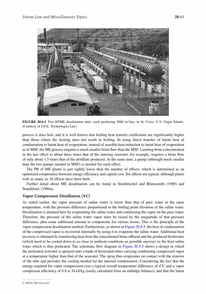
Patent Law and Miscellaneous Topics
20
-65
© 1999 by CRC Press LLC
process it does boil, and it is well known that boiling heat transfer coefÞcients are signiÞcantly higherthan those where the heating does not result in boiling. In using direct transfer of latent heat ofcondensation to latent heat of evaporation, instead of sensible heat reduction to latent heat of evaporationas in MSF, the ME process requires a much smaller brine ßow than the MSF. Limiting brine concentrationin the last effect to about three times that of the entering seawater, for example, requires a brine ßowof only about 1.5 times that of the distillate produced. At the same time, a pump (although much smallerthan the two pumps needed in MSF) is needed for each effect.
The PR of ME plants is just sightly lower than the number of effects, which is determined as anoptimized compromise between energy efÞciency and capital cost. Six effects are typical, although plantswith as many as 18 effects have been built.
Further detail about ME desalination can be found in Steinbruchel and Rhinesmith (1980) andStandiford, (1986a).
Vapor Compression Distillation (VC)
As stated earlier, the vapor pressure of saline water is lower than that of pure water at the sametemperature, with the pressure difference proportional to the boiling point elevation of the saline water.Desalination is attained here by evaporating the saline water and condensing the vapor on the pure water.Therefore, the pressure of the saline water vapor must be raised by the magnitude of that pressuredifference, plus some additional amount to compensate for various losses. This is the principle of thevapor compression desalination method. Furthermore, as shown in Figure 20.6.5, the heat of condensationof the compressed vapor is recovered internally by using it to evaporate the saline water. Additional heatrecovery is obtained by transferring heat from the concentrated brine efßuent and the produced freshwater(which need to be cooled down to as close to ambient conditions as possible anyway) to the feed salinewater which is thus preheated. The schematic ßow diagram in Figure 20.5.5 shows a design in whichthe preheated seawater is sprayed onto a bank of horizontal tubes carrying condensing compressed vaporat a temperature higher than that of the seawater. The spray thus evaporates on contact with the exteriorof the tube and provides the cooling needed for the internal condensation. Considering the fact that the
energy required for vapor compression over a typical overall temperature difference of 4
°
C and a vaporcompressor efÞciency of 0.8 is 34 kJ/kg (easily calculated from an enthalpy balance), and that the latent
FIGURE 20.6.3
Two HTME desalination units, each producing 5000 m
3
/day, in St. Croix, U.S. Virgin Islands.(Courtesy of I.D.E. Technologies Ltd.)
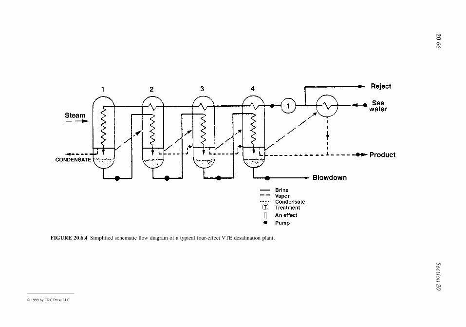
20-66Section
20
© 1999 by CRC Press LLC
FIGURE 20.6.4 SimpliÞed schematic ßow diagram of a typical four-effect VTE desalination plant.
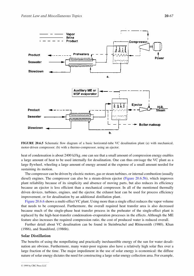
Patent Law and Miscellaneous Topics 20-67
© 1999 by CRC Press LLC
heat of condensation is about 2400 kJ/kg, one can see that a small amount of compression energy enablesa large amount of heat to be used internally for desalination. One can thus envisage the VC plant as alarge ßywheel, wheeling a large amount of energy around at the expense of a small amount needed forsustaining its motion.
The compressor can be driven by electric motors, gas or steam turbines, or internal combustion (usuallydiesel) engines. The compressor can also be a steam-driven ejector (Figure 20.6.5b), which improvesplant reliability because of its simplicity and absence of moving parts, but also reduces its efÞciencybecause an ejector is less efÞcient than a mechanical compressor. In all of the mentioned thermallydriven devices, turbines, engines, and the ejector, the exhaust heat can be used for process efÞciencyimprovement, or for desalination by an additional distillation plant.
Figure 20.6.6 shows a multi-effect VC plant. Using more than a single effect reduces the vapor volumethat needs to be compressed. Furthermore, the overall required heat transfer area is also decreasedbecause much of the single-phase heat transfer process in the preheater of the single-effect plant isreplaced by the high-heat-transfer condensationÐevaporation processes in the effects. Although the MEfeature also increases the required compression ratio, the cost of produced water is reduced overall.
Further detail about VC desalination can be found in Steinbruchel and Rhinesmith (1980), Khan(1986), and Standiford, (1986b).
Solar Distillation
The beneÞts of using the nonpolluting and practically inexhaustible energy of the sun for water desali-nation are obvious. Furthermore, many water-poor regions also have a relatively high solar ßux over alarge fraction of the time. The major impediment in the use of solar energy is economical: the diffusenature of solar energy dictates the need for constructing a large solar energy collection area. For example,
FIGURE 20.6.5 Schematic ßow diagram of a basic horizontal-tube VC desalination plant (a) with mechanical,motor-driven compressor; (b) with a thermo-compressor, using an ejector.

20-68 Section 20
© 1999 by CRC Press LLC
assuming a single-effect solar still efÞciency of 50% (which is the upper practical limit for conventionaldesigns), the still would produce at most about 3.5 to 4.8 kg fresh water per m2 per day, or a 208 to 286m2 solar still would be required to produce 1 m3 of fresh water per day. More realistic still efÞcienciesincrease the area requirement about twofold.
Shown in Figure 20.6.7, a typical solar still consists of a saline water container in which the water isexposed to the sun and heated by it. The temperature rise to above ambient causes net evaporation ofthe saline water, thus separating pure water vapor from the solution. The vapor condenses on the coldercover, and this destilled water ßows to collection troughs.
Solar stills of the type depicted in Figure 20.6.7, in many sizes and constructional variants, have beenbuilt and used successfully in many countries in the world. They are simple, easy to construct, reliable,and require very little maintenance although in some regions the covers must be cleaned frequently fromaccumulated dust or sand.
Since the heat of condensation in single-effect stills of the type shown in Figure 20.6.7 is lost to theambient, more-energy-efÞcient operation can obviously be achieved in a multi-effect design, where the
FIGURE 20.6.6 Schematic ßow diagram of a ME vapor compression submerged-tube desalinaton plant with threeeffects.
FIGURE 20.6.7 A typical basin-type solar still.
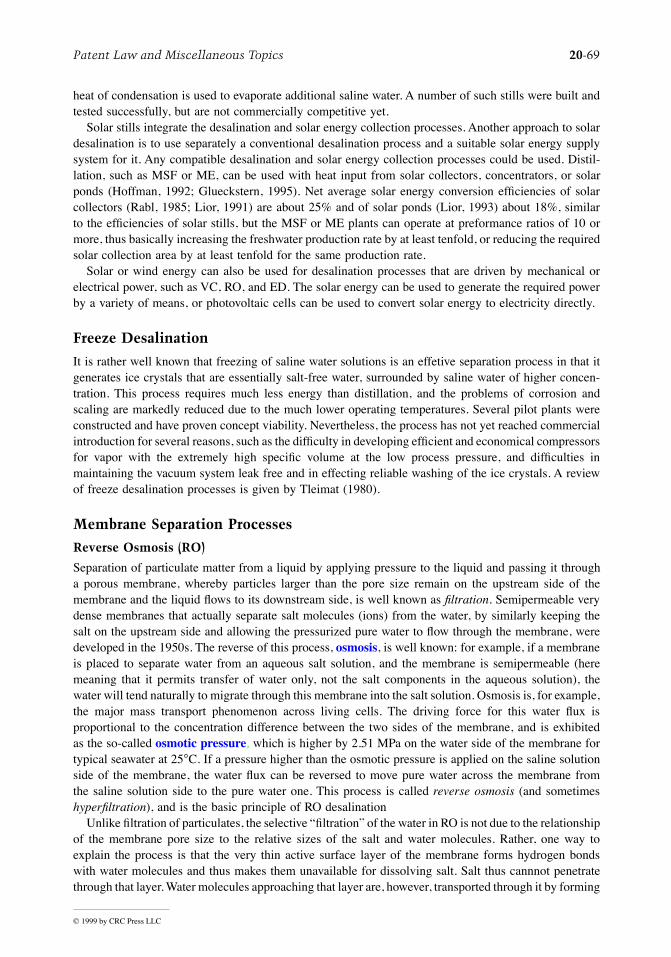
Patent Law and Miscellaneous Topics 20-69
© 1999 by CRC Press LLC
heat of condensation is used to evaporate additional saline water. A number of such stills were built andtested successfully, but are not commercially competitive yet.
Solar stills integrate the desalination and solar energy collection processes. Another approach to solardesalination is to use separately a conventional desalination process and a suitable solar energy supplysystem for it. Any compatible desalination and solar energy collection processes could be used. Distil-lation, such as MSF or ME, can be used with heat input from solar collectors, concentrators, or solarponds (Hoffman, 1992; Glueckstern, 1995). Net average solar energy conversion efÞciencies of solarcollectors (Rabl, 1985; Lior, 1991) are about 25% and of solar ponds (Lior, 1993) about 18%, similarto the efÞciencies of solar stills, but the MSF or ME plants can operate at preformance ratios of 10 ormore, thus basically increasing the freshwater production rate by at least tenfold, or reducing the requiredsolar collection area by at least tenfold for the same production rate.
Solar or wind energy can also be used for desalination processes that are driven by mechanical orelectrical power, such as VC, RO, and ED. The solar energy can be used to generate the required powerby a variety of means, or photovoltaic cells can be used to convert solar energy to electricity directly.
Freeze Desalination
It is rather well known that freezing of saline water solutions is an effetive separation process in that itgenerates ice crystals that are essentially salt-free water, surrounded by saline water of higher concen-tration. This process requires much less energy than distillation, and the problems of corrosion andscaling are markedly reduced due to the much lower operating temperatures. Several pilot plants wereconstructed and have proven concept viability. Nevertheless, the process has not yet reached commercialintroduction for several reasons, such as the difÞculty in developing efÞcient and economical compressorsfor vapor with the extremely high speciÞc volume at the low process pressure, and difÞculties inmaintaining the vacuum system leak free and in effecting reliable washing of the ice crystals. A reviewof freeze desalination processes is given by Tleimat (1980).
Membrane Separation Processes
Reverse Osmosis (RO)
Separation of particulate matter from a liquid by applying pressure to the liquid and passing it througha porous membrane, whereby particles larger than the pore size remain on the upstream side of themembrane and the liquid ßows to its downstream side, is well known as Þltration. Semipermeable verydense membranes that actually separate salt molecules (ions) from the water, by similarly keeping thesalt on the upstream side and allowing the pressurized pure water to ßow through the membrane, weredeveloped in the 1950s. The reverse of this process, osmosis, is well known: for example, if a membraneis placed to separate water from an aqueous salt solution, and the membrane is semipermeable (heremeaning that it permits transfer of water only, not the salt components in the aqueous solution), thewater will tend naturally to migrate through this membrane into the salt solution. Osmosis is, for example,the major mass transport phenomenon across living cells. The driving force for this water ßux isproportional to the concentration difference between the two sides of the membrane, and is exhibitedas the so-called osmotic pressure, which is higher by 2.51 MPa on the water side of the membrane fortypical seawater at 25°C. If a pressure higher than the osmotic pressure is applied on the saline solutionside of the membrane, the water ßux can be reversed to move pure water across the membrane fromthe saline solution side to the pure water one. This process is called reverse osmosis (and sometimeshyperÞltration), and is the basic principle of RO desalination
Unlike Þltration of particulates, the selective ÒÞltrationÓ of the water in RO is not due to the relationshipof the membrane pore size to the relative sizes of the salt and water molecules. Rather, one way toexplain the process is that the very thin active surface layer of the membrane forms hydrogen bondswith water molecules and thus makes them unavailable for dissolving salt. Salt thus cannnot penetratethrough that layer. Water molecules approaching that layer are, however, transported through it by forming
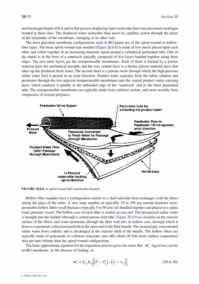
20-70 Section 20
© 1999 by CRC Press LLC
such hydrogen bonds with it and in that process displacing water molecules that were previously hydrogenbonded at these sites. The displaced water molecules then move by capillary action through the poresof the remainder of the membrane, emerging at its other side.
The most prevalent membrane conÞgurations used in RO plants are of the spiral-wound or hollow-Þber types. The basic spiral-wound-type module (Figure 20.6.8) is made of two sheets placed upon eachother and rolled together in an increasing diameter spiral around a cylindrical perforated tube. One ofthe sheets is in the form of a sandwich typically composed of Þve layers bonded together along threeedges. The two outer layers are the semipermeable membranes. Each of them is backed by a porousmaterial layer for mechanical strength, and the very central layer is a thicker porous material layer thattakes up the produced fresh water. The second sheet is a porous mesh through which the high-pressuresaline water feed is passed in an axial direction. Product water separates from the saline solution andpermeates through the two adjacent semipermeable membranes into the central product waterÐcarryinglayer, which conducts it spirally to the unbonded edge of the ÒsandwichÓ and to the inner perforatedtube. The semipermeable membranes are typically made from cellulose acetate, and more recently fromcomposites of several polymers.
Hollow Þber modules have a conÞguration similar to a shell-and-tube heat exchanger, with the Þberstaking the place of the tubes. A very large number of typicallly 25 to 250 mm outside-diameter semi-permeable hollow Þbers (wall thickness typically 5 to 50 mm) are bundled together and placed in a salinewater pressure vessel. The hollow core of each Þber is sealed on one end. The pressurized saline wateris brought into the module (through a central porous feed tube, Figure 20.6.9) to circulate on the exteriorsurface of the Þbers, and water permeates through the Þber wall into its hollow core, through which itßows to a permeate collection manifold at the open end of the Þber bundle. The increasingly concentratedsaline water ßows radially and is discharged at the exterior shell of the bundle. The hollow Þbers aretypically made of polyamide or cellulose triacetate, and offer about 20 fold more surface (separation)area per unit volume than the spiral-wound conÞguration.
The basic approximate equation for the separation process gives the water ßux (kg/m2sec) acrossan RO membrane, in the absence of fouling, as
(20.6.10)
FIGURE 20.6.8 A spiral-wound RO membrane element.
Ç¢¢mw
Ç¢¢ = -( ) - -( )[ ]m K K P Pw pe cf f p f pp p
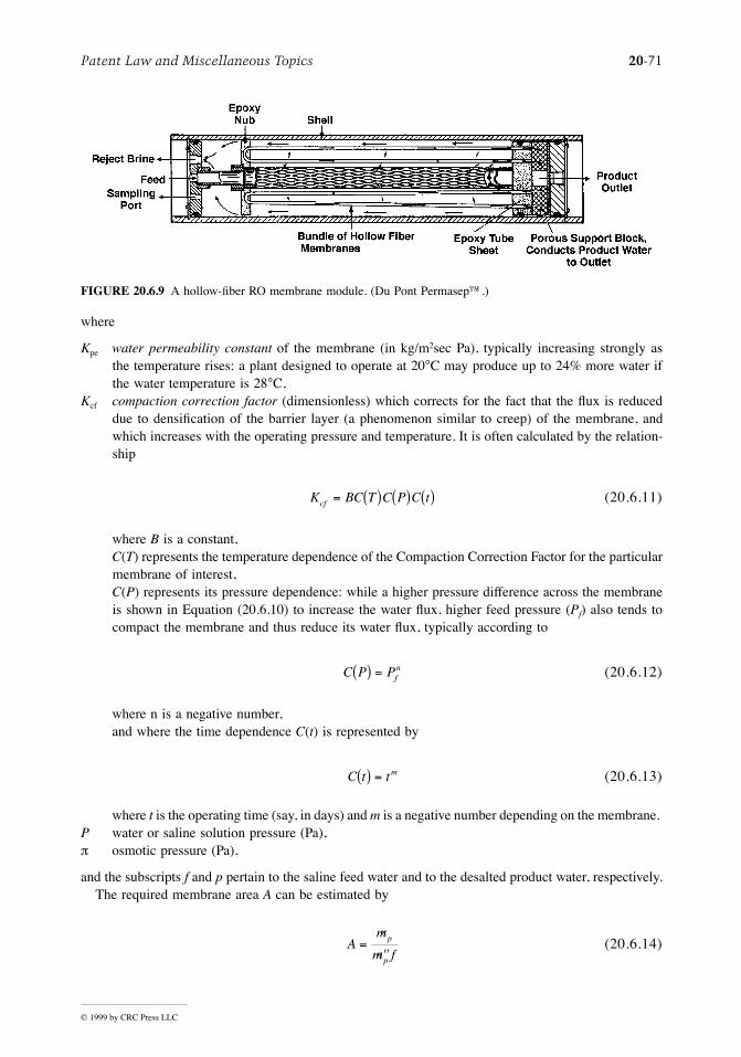
Patent Law and Miscellaneous Topics 20-71
© 1999 by CRC Press LLC
where
Kpe water permeability constant of the membrane (in kg/m2sec Pa), typically increasing strongly asthe temperature rises: a plant designed to operate at 20°C may produce up to 24% more water ifthe water temperature is 28°C,
Kcf compaction correction factor (dimensionless) which corrects for the fact that the ßux is reduceddue to densiÞcation of the barrier layer (a phenomenon similar to creep) of the membrane, andwhich increases with the operating pressure and temperature. It is often calculated by the relation-ship
(20.6.11)
where B is a constant,C(T) represents the temperature dependence of the Compaction Correction Factor for the particularmembrane of interest,C(P) represents its pressure dependence: while a higher pressure difference across the membraneis shown in Equation (20.6.10) to increase the water ßux, higher feed pressure (Pf) also tends tocompact the membrane and thus reduce its water ßux, typically according to
(20.6.12)
where n is a negative number,and where the time dependence C(t) is represented by
(20.6.13)
where t is the operating time (say, in days) and m is a negative number depending on the membrane. P water or saline solution pressure (Pa),p osmotic pressure (Pa),
and the subscripts f and p pertain to the saline feed water and to the desalted product water, respectively.The required membrane area A can be estimated by
(20.6.14)
FIGURE 20.6.9 A hollow-Þber RO membrane module. (Du Pont Permasepª.)
K BC T C P C tcf = ( ) ( ) ( )
C P Pfn( ) =
C t tm( ) =
Am
m fp
p
=¢¢
Ç
Ç
20-72 Section 20
© 1999 by CRC Press LLC
where is the freshwater mass production rate of the plant (kg/sec), and f (0 < f £ 1.0) is the areautilization factor that corrects for the fact that the membrane surface is incompletely in contact with thesaline water feed stream due to the porous mesh and other devices, such as turbulence promoters, placedin the feed stream path; in a good design f > 0.9.
Examination of Equation (20.6.10) shows that water separation rate increases with the water perme-ability constant Kpe. Unfortunately, so does the salt ßux across the membrane, resulting in a saltierproduct. An approximation for this salt ßow is
(20.6.15)
where
salt mass transfer rate across the membrane, kg/sec,K a proportionality constant, dimensionless,Ks salt permeation constant, kg/sec, which increases with pressure and temperature.
The salinity of the product water (Cp) can be estimated by the formula
(20.6.16)
where
Kcp concentration polarization coefÞcient, º is a measure of the increase of the feedwatersalinity at the membrane wall beyond that of the bulk solution,
Cfm salt concentration at the membrane wall,
bulk salinity of the saline water feed, » (Cf + Cr)/2,Cr salt concentration of the reject brine,h salt rejection factor, º (amount of salts rejected by the membrane)/(amount of salts in the brine
feed).
The pressure to be used for RO depends on the salinity of the feed water, the type of membrane, andthe desired product purity. It ranges form about 1.5 MPa for low feed concentrations or high-ßuxmembranes, through 2.5 to 4 MPa for brackish waters, and to 6 to 8.4 MPa for seawater desalination.In desalination of brackish water, typical product water ßuxes through spiral-wound membranes areabout 600 to 800 kg/(m2day) at a recovery ratio (RR) of 15% and an average salt rejection of 99.5%, where
(20.6.17)
The ßuxes in hollow-Þber membranes used in seawater desalination are 20- to 30-fold smaller, butthe overall RO system size does not increase, because the hollow-Þber membranes have a much largersurface area per unit volume. The RR and salt rejection ratio are similar to those of spiral-woundmembranes.
Since the concentrated reject brine is still at high pressure, it is possible to recover energy by passingthis brine through hydraulic turbines, and thus reduce the overall energy consumption by up to 20%.The energy requirements of seawater RO desalination plants with energy recovery are about 5 to 9 kWh,or 18 to 33 MJ, of mechanical or electric power per m3 fresh water produced. In comparison, the MSFdesalination process requires about 120 to 280 MJ of heat and about 15 MJ of mechanical/electric power(for pumping and auxiliaries) per m3. The energy requirement of the RO process is thus smaller thanthat of the MSF process even if the RO energy requirement is multiplied by the thermal-to-mechanical
Çmp
Çm KK C Cs s fm p= -( )
Çms
C K Cp cp= -( )1 h
C Cfm /
C
RR = @ -Ç
Ç
m
m
C
Cp
f
f
r
1
Patent Law and Miscellaneous Topics 20-73
© 1999 by CRC Press LLC
(or electrical) power conversion factor of 3 to 4. The speciÞc exergy consumption of the MSF processusing 120°C steam is about 2- to 3-fold higher than that of the RO process, but becomes comparable inmagnitude if the steam temperature is lowered to 80°C.
The life of membranes is affected by gradual chemical decomposition or change. For example,cellulose acetate membranes hydrolyze with time. The rate of hydrolysis has a steep minimum at asolution pH of 4.5 to 5.0, and increases drastically with temperature.
Membranes are susceptible to plugging by dirt and to deterioration in their selectivity caused byvarious species present in the saline water. Careful pretreatment of the feed water is therefore necessary.It typically consists of clariÞcation, Þltration, chlorination for destroying organic matter and microor-ganisms, removal of excess chlorine to prevent membrane oxidation, and dosing with additives to preventcalcium sulfate scaling and foam formation. Periodical chemical or mechanical cleaning is also necessary.Pretreatment and cleaning are signiÞcant and increasing fractions of the RO plant capital and operatingcosts.
Further detail about RO desalination can be found in Sourirajan and Matsuura (1985) and Amjad(1993).
Electrodialysis (ED)
In ED, the saline solution is placed between two membranes, one permeable to cations only and theother to anions only. A direct electrical current is passed across this system by means of two electrodes,cathode and anode, exposed to the solution (Figure 20.6.10). It causes the cations in the saline solutionto move toward the cathode, and the anions to the anode. As shown in Figure 20.6.10, the anions canleave the compartment in their travel to the anode because the membrane separating them from theanode is permeable to them. Cations would similarly leave the compartment toward the cathode. Theexit of these ions from the compartment reduces the salt concentration in it, and increases the saltconcentration in the adjacent compartments. Tens to hundreds of such compartments are stacked togetherin practical ED plants, leading to the creation of alternating compartments of fresh and salt-concentratedwater. ED is a continuous-ßow process, where saline feed is continuously fed into all compartments andthe product water and concentrated brine ßow out of alternate compartments. The ßow along themembranes also improves the mass transport there, and the separators between the membranes areconstructed to provide good ßow distribution and mixing on the membrane surfaces. Membrane sizesare roughly 0.5 ´ 1 m, spaced about 1 mm apart. Many typed of polymers are used to manufacture theseion-exchange selective membranes, which are often reinforced by strong fabrics made from otherpolymers or glass Þbers.
Careful and thorough feed water pretreatment similar to that described in the section on RO is required.Pretreatment needs and operational problems of scaling are diminished in the electrodialysis reversal(EDR) process, in which the electric current ßow direction is periodically reversed (say, three to fourtimes per hour), with simultaneous switching of the water ßow connections. This also reverses the saltconcentration buildup at the membrane and electrode surfaces, and prevents concentrations that causethe precipitation of salts and scale deposition.
The voltage used for ED is about 1 V per membrane pair, and the current ßux is of the order of 100A/m2 of membrane surface. The total power requirement increases with the feed water salt concentration,amounting to about 10 MW/m3 product water per 1000 ppm reduction in salinity. About half this poweris required for separation and half for pumping. Many plant ßow arrangements exist, and their descriptioncan be found, along with other details about the process, in Shaffer and Mintz (1980) and Heitman (1991).
Defining Terms
Boiling point elevation: The number of degrees by which the boiling point temperature of a solutionis higher than that of the pure solute at the same pressure.Flash evaporation: An evaporation process that occurs when a liquid with a free surface is exposed toits vapor, where the vapor is below the saturation pressure corresponding to the temperature of the liquid.
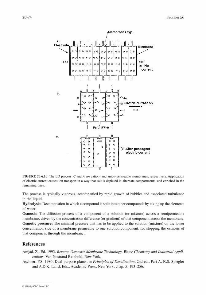
20-74 Section 20
© 1999 by CRC Press LLC
The process is typically vigorous, accompanied by rapid growth of bubbles and associated turbulencein the liquid.Hydrolysis: Decompostion in which a compound is split into other compounds by taking up the elementsof water.Osmosis: The diffusion process of a component of a solution (or mixture) across a semipermeablemembrane, driven by the concentration difference (or gradient) of that component across the membrane.Osmotic pressure: The minimal pressure that has to be applied to the solution (mixture) on the lowerconcentration side of a membrane permeable to one solution component, for stopping the osmosis ofthat component through the membrane.
References
Amjad, Z., Ed. 1993. Reverse Osmosis: Membrane Technology, Water Chemistry and Industrial Appli-cations. Van Nostrand Reinhold, New York.
Aschner, F.S. 1980. Dual purpose plants, in Principles of Desalination, 2nd ed., Part A, K.S. Spieglerand A.D.K. Laird, Eds., Academic Press, New York, chap. 5, 193Ð256.
FIGURE 20.6.10 The ED process. C and A are cation- and anion-permeable membranes, respectively. Applicationof electric current causes ion transport in a way that salt is depleted in alternate compartments, and enriched in theremaining ones.

Patent Law and Miscellaneous Topics 20-75
© 1999 by CRC Press LLC
Burns and Roe, Inc, 1969. Universal DesignÑReport and UserÕs Manual on Design of 2.5 MillionGallon per Day Universal Desalting Plant, Vols. IÐV, U.S. Department of the Interior, O.S.W.Contract No. 14-01-0001-955, Washington, D.C.
Fabuss, B.M. 1980. Properties of seawater, in Principles of Desalination, 2nd ed., Part B, K. S. Spieglerand A.D.K. Laird, Eds., Academic Press, New York, Appendix 2, 765Ð799.
George P.F., Manning, J.A., and Schrieber, C.F. 1975. Desalinatin Materials Manual. U.S. Departmentof the Interior, OfÞce of Saline Water, Washington, D. C.
Glater, J., York, J.L., and Campbell, K.S. 1980. Scale formation and prevention, in Principles ofDesalination, 2nd ed., Part B, K.S. Spiegler and A.D.K. Laird, Eds., Academic Press, New York,chap. 10, 627Ð678.
Glueckstern, P. 1995, Potential uses of solar energy for seawater desalination, Desalination, 101, 11Ð20.Heitman, H.-G. 1990. Saline Water Processing, VCH Publications, New York.Hoffman, D. 1992. The application of solar energy for large scale sea water desalination, Desalination,
89, 115Ð184.Kasper, S.P. and Lior, N. 1979. A methodology for comparing water desalination to competitive fresh-
water transportation and treatment, Desalination, 30, 541Ð552.Khan, A.S. 1986. Desalination Processes and Multistage Flash Distillation Practice, Elsevier, Amster-
dam.Lior, N., Ed. 1986. Measurements and Control in Water Desalinaion, Elsevier, Amsterdam.Lior, N. 1991. Thermal theory and modeling of solar collectors, in Solar Collectors, Energy Storage,
and Materials, F. de Winter, Ed., MIT Press, Cambridge, MA, chap. 4, 99Ð182.Lior, N. 1993. Research and new concepts, in Active Solar Systems, G.O.G. L�f, Ed., MIT Press,
Cambridge, MA, chap. 17, 615Ð674.Lior, N. and Greif, R, 1980. Some basic observations on heat transfer and evaporation in the horizontal
ßash evaporator, Desalination, 33, 269Ð286.Miyatake, O., Hashimoto, T., and Lior, N. 1992. The liquid ßow in multi-stage ßash evaporators, Int. J.
Heat Mass Transfer, 35, 3245Ð3257.Miyatake, O., Hashimoto, T., and Lior, N. 1993. The relationship between ßow pattern and thermal non-
equilibrium in the multi-stage ßash evaporation process, Desalination, 91, 51Ð64.M.W. Kellogg Co. 1975. Saline Water Data Conversion Engineering Data Book, 3rd ed., U.S. Department
of the Interior, OfÞce of Saline Water Contract No. 14-30-2639, Washington, D.C.Rabl, A. 1985. Active Solar Collectors and Their Applications, Oxford University Press, New York.Shaffer, L.H. and Mintz, M.S. 1980. Electrodialysis, in Principles of Desalination, 2nd ed., Part A, K.S.
Spiegler and A.D.K. Laird, Eds., Academic Press, New York, chap. 6, 257Ð357.Sourirajan, S. and Matsuura, T., Eds. 1985. Reverse Osmosis and UltraÞltration, ACS Symposium Series
281, American Chemical Society, Washington, D.C.Spiegler, K.S. and El-Sayed, Y.M. 1994. A Desalination Primer. Balaban Desalination Publications,
Mario Negri Sud Research Institute, 66030 Santa Maria Imbaro (Ch), Italy.Spiegler, K.S. and Laird, A.D.K., Eds. 1980. Principles of Desalination, 2nd ed., Academic Press, New
York.Standiford, F.C. 1986a. Control in multiple effect desalination plants, in Measurements and Control in
Water Desalination, N. Lior, Ed., Elsevier, Amsterdam, chap. 2.2, 263Ð292.Standiford, F.C. 1986b. Control in vapor compression evaporators, in Measurements and Control in
Water Desalination, N. Lior, Ed., Elsevier, Amsterdam, chap. 2.3, 293Ð306.Steinbruchel, A.B. and Rhinesmith, R.D. 1980. Design of distilling plants, in Principles of Desalination,
2nd ed., Part A, K.S. Spiegler and A.D.K. Laird, Eds., Academic Press, New York, chap. 3,111Ð165.
Tleimat, B.W. 1980. Freezing methods, in Principles of Desalination, 2nd ed., Part B, K.S. Spiegler andA.D.K. Laird, Eds., Academic Press, New York, chap. 7, 359Ð400.

20-76 Section 20
© 1999 by CRC Press LLC
Further Information
The major texts on water desalination written since the 1980s are Spiegler and Laird (1980), Khan,(1986) (contains many practical design aspects), Lior (1986) (on the measurements and control aspects),Heitman (1990) (on pretreatment and chemistry aspects), and Spiegler and El-Sayed (1994) (an overiewprimer). Extensive data sources are provided in George et al. (1975) and M. W. Kellog (1975).
The two major professional journals in this Þeld are Desalination, The International Journal on theScience and Technology of Desalting and Water PuriÞcation and Membrane Science, which oftenaddresses membrane-based desalination processes, both published by Elsevier, Amsterdam.
The major professional society in the Þeld is the International Desalination Association (IDA) head-quartered at P.O. Box 387, TopsÞeld, MA 01983. IDA regularly organizes international conferences,promotes water desalinaton and reuse technology, and is now publishing a trade magazine The Interna-tional Desalination & Water Reuse Quarterly.
The Desalination Directory by M. Balaban Desalination Publications, Mario Negri Sud ResearchInstitute, 66030 Santa Maria Imbaro (Ch), Italy, lists more than 5000 individuals and 2000 companiesand institutions in the world of desalinaiton and water reuse.
Two useful (though by now somewhat dated) books on desalination are by Howe, E. D. 1974.Fundamentals of Water Desalination, Marcel Dekker, New York, and by Porteous, A. 1975. Saline WaterDistillation Processes, Longman, London.
Much information on oceans and seawater properties is avaiable in the book by Riley, J. P. and Skinner,Eds. 1975. Chemical Oceanography, Academic Press, New York.
Patent Law and Miscellaneous Topics 20-77
© 1999 by CRC Press LLC
20.7 Noise Control
Malcolm J. Crocker
Introduction
Noise is usually deÞned as unwanted sound. Noise in industry experienced over an extended period cancause hearing loss. Noise in other environments Ñ in buildings, vehicles, and communities from avariety of sources causes speech interference, sleep disturbance, annoyance, and other effects (Crocker,1997b,d). Noise propagates as sound waves in the atmosphere and as vibration in buildings, machinery,vehicles, and other structures. Noise can be controlled at the source, in the path, or at the receiver. Theear is more sensitive to noise in the mid- to high-frequency range, but fortunately high-frequency iseasier to control than low-frequency noise. Several passive methods of noise and vibration control aredescribed. An example of successful noise control is the considerable reduction in passenger jet aircraftnoise in the last several years which has made them considerably quieter.
Sound Propagation
Sound waves propagate rather like ripples on a lake when a stone is thrown in (Crocker, 1997c). Theripples spread out from the source of the disturbance as circular waves until they reach a solid body orboundary (such as the lake edge) where reßections occur. The water does not ßow from the source, butthe disturbance propagates in the form of momentum and energy which is eventually dissipated. Soundwaves in air cannot be seen but behave in a similar manner. Sound waves propagating in three dimensionsfrom a source of sound are spherical rather than circular like the two-dimensional water wave propagation.Sound waves propagate at the wave speed (or sound speed c) which is dependent only on the absolutetemperature T. It is 343 m/sec (1120 ft/sec) at a normal atmospheric temperature of 20°C. The wavelengthl of sound is inversely proportional to the frequency f in cycles/sec (known as hertz or Hz) and is givenby l = c/f Hz. The sound waves result in ßuctuations in the air pressure as they propagate. The airpressure difference from the mean atmospheric pressure is deÞned as the sound pressure. A logarithmicmeasure, the sound pressure level SPL or Lp, is usually used with sound and noise and the units aredecibels (dB). The sound pressure level is Lp = 10 log10 where p is the rms sound pressureand pref is the reference sound pressure 20 mPa (or 20 ´ 10Ð6 N/m2). See Figure 20.7.1 (Crocker, 1997c).
Human Hearing
The human ear has a wide frequency response from about 15 or 20 Hz to about 16,000 Hz (Crocker,1975; Greenberg, 1997). The ear also has a large dynamic range; the ratio of the loudest sound pressurewe can tolerate to the quietest sound that we can hear is about ten million (107). This is equivalent to140 dB. The ear can be divided into three main parts: the outer, middle, and inner ear. The outer ear,consisting of the ßeshy pinna and ear canal, conducts the sound waves onto the ear drum. The middleear converts the sound pressure at the ear drum into the mechanical motion of three small bones (namedauditory ossicles: malleus, incus, and stapes) which in turn convert the mechanical motion into wavesin the inner ear. Hair cells in the inner ear respond to the excitation and send neural impulses along theauditory nerves to the brain (Figure 20.7.2).
The higher the sound pressure level of a sound, the louder it normally sounds, although the frequencycontent of the sound is important too. The ear is most sensitive to sound in the mid-frequency rangeand hears sound only poorly at lower frequencies (below 200 or 300 Hz). Most people have a maximumsensitivity to sound at about 4000 Hz (corresponding to a quarter wave resonance in the ear canal, witha pressure maximum at the eardrum). Electrical Þlters have been produced corresponding approximatelyto the frequency response of the ear. The A-weighting Þlter is the one most used and it Þlters off aconsiderable amount of the sound energy at low frequencies. The sound pressure level measured withan A-weighting Þlter is normally known as the A-weighted sound level (or the sound level for short).
( / ),p p2ref2

20-78 Section 20
© 1999 by CRC Press LLC
FIGURE 20.7.1 Some typical sound pressure levels.
FIGURE 20.7.2 Cross section of the human ear showing the three main parts: outer, middle, and inner ear.

Patent Law and Miscellaneous Topics 20-79
© 1999 by CRC Press LLC
The anatomy and functioning of the ear are described more completely in several books (Crocker, 1997;Greenberg, 1997).
Noise Measures
There are several rating measures and descriptors used to determine human response to noise. Only afew of the most important can be discussed here. The reader will Þnd more such measures discussed inthe literature. [1] Criteria derived from such measures can be used to produce regulations or legislation.
The speech interference level (SIL) is a measure used to evaluate the effect of background noise onspeech communication. The SIL is the arithmetic average of the sound pressure levels of the interferingbackground noise in the four octave bands with center frequencies of 500, 1000, 2000 and 4000 Hz.1,6
The speech interference level of the background noise is calculated; then this may be used inconjunction with Figure 20.7.3 to determine if communication is possible at various distances for differentvoice levels. This Þgure is for male voices. Since the average female voice is normally quieter, for femalevoices the horizontal scale should be moved to the right by 5 dB. Use of the results obtained with Figure20.7.3 and criteria for various spaces in buildings enable decisions to be made whether they are suitablefor their desired uses.
The equivalent sound level Leq is the A-weighted sound pressure level averaged over a suitable timeperiod T. The averaging time T can be chosen to be a number of minutes, hours or days, as desired.
where pA is the instantaneous sound pressure measured using an A-weighting frequency Þlter. The Leq
is also sometimes known as the average sound level LAT.
FIGURE 20.7.3 Recommended distances between speaker and listener for various voice levels for just reliablespeech communication. (From C.M. Harris Handbook of Noise Control, McGraw-Hill, New York, 1979. Withpermission.)
L T p dt p dBAeq ref2= ( )é
ëêùûúò10 110
2log

20-80 Section 20
© 1999 by CRC Press LLC
The day-night equivalent sound level (DNL) or Ldn is a measure that accounts for the different humanresponse to sound at night. It is deÞned (Crocker, 1997d) as:
where Ld is the 15-hr daytime A-weighted equivalent sound level (from 0700 to 2200 hr) and Ln is the9-hr nighttime equivalent sound level (from 2200 to 0700 hr). The nighttime level is subjected to a 10-dB penalty because noise at night is known to be more disturbing than noise during the day.
There is some evidence that noise that ßuctuates markedly in level is more annoying than noise whichis steady in level. Several noise measures have been proposed to try to account for the annoying effectof these ßuctuations. The percentile levels are used in some measures. The percentile level Ln is deÞnedto be the level exceeded n% of the time (Crocker, 1997d). The A-weighted sound level is normally usedin Ln.
Response of People to Noise and Noise Criteria and Regulations
In industry, noise is often intense enough to interfere with speech and to create noise conditions that arehazardous to hearing. By using Figure 20.7.3 it is seen that if the SIL is above 50 dB, then the noisewill interfere with normal speech communication between male voices at 4 m. If it is above 60 dB, thenspeech communication even when shouting is barely possible at the same distance. For women thecomparable values of SIL are 45 and 55 dB at the same distance. If the SIL is 90 dB, then communicationbetween male voices is only possible at distances less than 0.25 m, even when shouting. A-weightedsound levels are sometimes used instead of SIL values but with somewhat less conÞdence. It is seenthat if one has difÞculty in communicating in an industrial situation, then the A-weighted sound levelis likely to be above 90 dB. In the United States, OSHA regulations start at this level for an 8-hr period.There is a halving in the allowable exposure time for every 5-dB increase in sound level. See Table20.7.1. In almost all other countries the allowable exposure time is halved for every 3-dB increase insound level (Ward, 1997).
Noise in communities is caused by many different sources. In most countries, the maximum equivalentA-weighted sound level Leq is recommended for evaluating different types of noise source (Gottlob,1995). In some countries there are regulations which use Leq for road trafÞc noise and railroad noise,although some countries use L10 (e.g., the U.K.) or L50 (e.g., Japan) for planning permission in whichroad trafÞc noise is of concern (Crocker, 1997d; Gottlob, 1995). In the United States the Ldn has beenused for community noise situations involving aircraft noise at airports and road trafÞc noise. Table20.7.2 presents levels of noise given by the U.S. EPA and several other bodies to protect public health.
TABLE 20.7.1 Maximum A-Weighted Sound Levels Allowed by the U.S. Occupational Safety and Health Administration (OSHA) for Work Periods Shown during a Workday
Duration per Day (hr) Sound Level in dB(A)
8 906 924 953 972 1001.5 1021 1050.5 1100.25 or less 115
L dBL Ld ndn = ( ) ( ) + ( )é
ëêùûú
ìíî
üýþ
+( )10 1 24 15 10 9 101010 10 10log
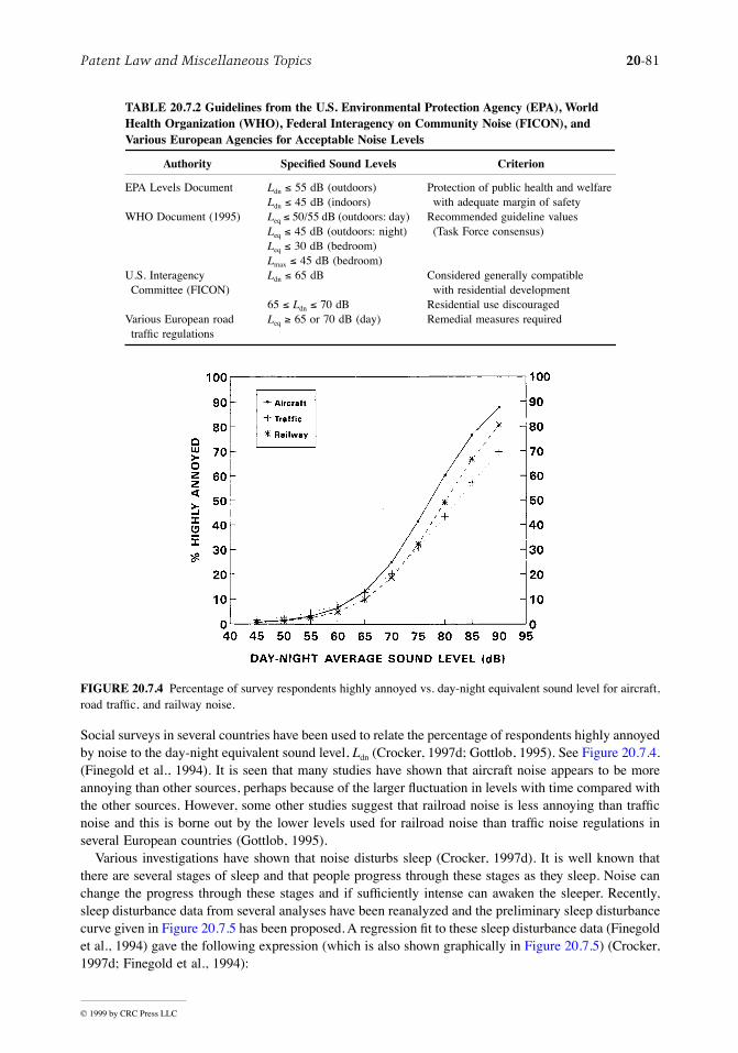
Patent Law and Miscellaneous Topics 20-81
© 1999 by CRC Press LLC
Social surveys in several countries have been used to relate the percentage of respondents highly annoyedby noise to the day-night equivalent sound level, Ldn (Crocker, 1997d; Gottlob, 1995). See Figure 20.7.4.(Finegold et al., 1994). It is seen that many studies have shown that aircraft noise appears to be moreannoying than other sources, perhaps because of the larger ßuctuation in levels with time compared withthe other sources. However, some other studies suggest that railroad noise is less annoying than trafÞcnoise and this is borne out by the lower levels used for railroad noise than trafÞc noise regulations inseveral European countries (Gottlob, 1995).
Various investigations have shown that noise disturbs sleep (Crocker, 1997d). It is well known thatthere are several stages of sleep and that people progress through these stages as they sleep. Noise canchange the progress through these stages and if sufÞciently intense can awaken the sleeper. Recently,sleep disturbance data from several analyses have been reanalyzed and the preliminary sleep disturbancecurve given in Figure 20.7.5 has been proposed. A regression Þt to these sleep disturbance data (Finegoldet al., 1994) gave the following expression (which is also shown graphically in Figure 20.7.5) (Crocker,1997d; Finegold et al., 1994):
TABLE 20.7.2 Guidelines from the U.S. Environmental Protection Agency (EPA), World Health Organization (WHO), Federal Interagency on Community Noise (FICON), and Various European Agencies for Acceptable Noise Levels
Authority SpeciÞed Sound Levels Criterion
EPA Levels Document Ldn £ 55 dB (outdoors)Ldn £ 45 dB (indoors)
Protection of public health and welfare with adequate margin of safety
WHO Document (1995) Leq £ 50/55 dB (outdoors: day)Leq £ 45 dB (outdoors: night)Leq £ 30 dB (bedroom)Lmax £ 45 dB (bedroom)
Recommended guideline values(Task Force consensus)
U.S. Interagency Committee (FICON)
Ldn £ 65 dB Considered generally compatiblewith residential development
65 £ Ldn £ 70 dB Residential use discouragedVarious European road trafÞc regulations
Leq ³ 65 or 70 dB (day) Remedial measures required
FIGURE 20.7.4 Percentage of survey respondents highly annoyed vs. day-night equivalent sound level for aircraft,road trafÞc, and railway noise.
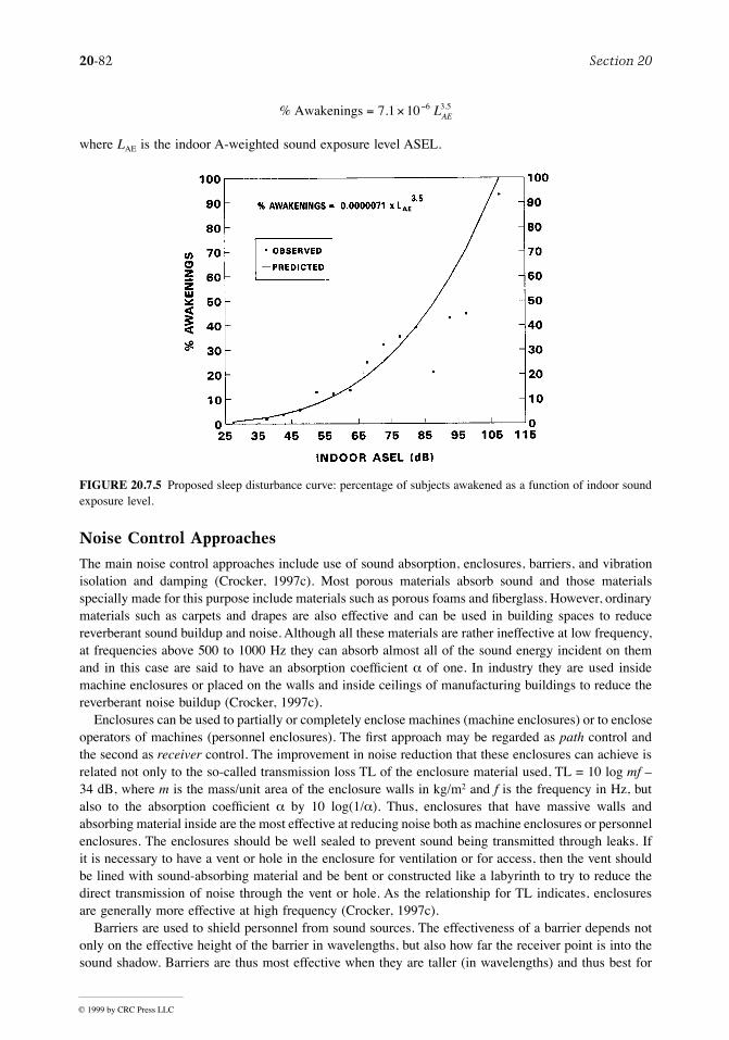
20-82 Section 20
© 1999 by CRC Press LLC
where LAE is the indoor A-weighted sound exposure level ASEL.
Noise Control Approaches
The main noise control approaches include use of sound absorption, enclosures, barriers, and vibrationisolation and damping (Crocker, 1997c). Most porous materials absorb sound and those materialsspecially made for this purpose include materials such as porous foams and Þberglass. However, ordinarymaterials such as carpets and drapes are also effective and can be used in building spaces to reducereverberant sound buildup and noise. Although all these materials are rather ineffective at low frequency,at frequencies above 500 to 1000 Hz they can absorb almost all of the sound energy incident on themand in this case are said to have an absorption coefÞcient a of one. In industry they are used insidemachine enclosures or placed on the walls and inside ceilings of manufacturing buildings to reduce thereverberant noise buildup (Crocker, 1997c).
Enclosures can be used to partially or completely enclose machines (machine enclosures) or to encloseoperators of machines (personnel enclosures). The Þrst approach may be regarded as path control andthe second as receiver control. The improvement in noise reduction that these enclosures can achieve isrelated not only to the so-called transmission loss TL of the enclosure material used, TL = 10 log mf Ð34 dB, where m is the mass/unit area of the enclosure walls in kg/m2 and f is the frequency in Hz, butalso to the absorption coefÞcient a by 10 log(1/a). Thus, enclosures that have massive walls andabsorbing material inside are the most effective at reducing noise both as machine enclosures or personnelenclosures. The enclosures should be well sealed to prevent sound being transmitted through leaks. Ifit is necessary to have a vent or hole in the enclosure for ventilation or for access, then the vent shouldbe lined with sound-absorbing material and be bent or constructed like a labyrinth to try to reduce thedirect transmission of noise through the vent or hole. As the relationship for TL indicates, enclosuresare generally more effective at high frequency (Crocker, 1997c).
Barriers are used to shield personnel from sound sources. The effectiveness of a barrier depends notonly on the effective height of the barrier in wavelengths, but also how far the receiver point is into thesound shadow. Barriers are thus most effective when they are taller (in wavelengths) and thus best for
FIGURE 20.7.5 Proposed sleep disturbance curve: percentage of subjects awakened as a function of indoor soundexposure level.
% Awakenings = ´ -7 1 10 6 3 5. .LAE
Patent Law and Miscellaneous Topics 20-83
© 1999 by CRC Press LLC
high-frequency noise and also best when placed close to the source or close to the receiver, since suchplacement increases the shadowing effect. Barriers are used in industry where it is desired to shieldpersonnel from machinery noise sources. It is important in such cases to put sound-absorbing materialon the ceiling of the building just above the barrier or on walls just behind a barrier where these surfacescould allow the reßection of sound to bypass the barrier and thus severely reduce its effectiveness(Crocker, 1997c).
The vibration isolation of machine sources from their supports can be particularly useful in reducingthe noise produced especially if the machine is small compared with a large ßexible support or enclosurethat can act as a sounding board and radiate the sound. Soft metal springs or elastomeric isolators areoften used as isolators. They should be designed so that the natural frequency of the machine mass onits isolators is much less than the forcing frequency, if possible. Care should be taken that such a designcondition does not produce excessive static deßection of the system that could interfere with the propermachine operation. Vibrating pipes and ducts can also be vibration-isolated from walls of buildings usingpipe hangers or soft rubber isolators. Vibration breaks made of rubber or similar soft material can bebuilt into elements such as walls in buildings or structural elements in vehicles or machine enclosuresto prevent vibration being propagated throughout the building or other structure and being reradiated asnoise (Crocker, 1997c).
Damping materials can also be effective at reducing noise when applied properly to structures if theirvibration is resonant in nature. Damping materials that are viscous, applied with thicknesses two or threetimes that of the vibrating metal panel, are particularly effective. Constrained damping layers can bevery effective even when the damping layer is relatively thin (Crocker, 1997c).
Figure 20.7.6 shows the reduction in the A-weighted sound level that can be expected using thesepassive noise control approaches discussed above. Often it is insufÞcient to use one approach, and greater,more-economic noise reduction can be achieved by using two or more approaches in conjunction.
References
Beranek, L.L. and Ver, I.L. 1992. Noise and Vibration Control Engineering, John Wiley & Sons, NewYork.
Crocker, M.J. 1975. in Noise and Noise Control, CRC Press, Cleveland, OH, chap. 2.Crocker, M.J. 1997a. Introduction to linear acoustics, in Encyclopedia of Acoustics, M.J. Crocker, Ed.,
John Wiley & Sons, New York, chap. 1.Crocker, M.J. 1997b. Noise, in Handbook of Human Factors and Ergonomics, 2nd ed., G. Salvendy,
Ed., John Wiley & Sons, New York, chap. 24.Crocker, M.J. 1977c. Noise generation in machinery, its control and source identiÞcation, in Encyclopedia
of Acoustics, M.J. Crocker, Ed., John Wiley & Sons, New York, chap. 83.Crocker, M.J. 1997d. Rating measures, criteria, and procedures for determining human response to noise,
in Encyclopedia of Acoustics, M.J. Crocker, Ed., John Wiley & Sons, New York, chap. 80.Finegold, L.S., Harris, C.S., and von Gierke, H.E. 1994. Community annoyance and sleep disturbance:
updated criteria for assessment of the impacts of general transportation noise on people, NoiseControl Eng. J., 42(1), 25Ð30.
Gottlob, D. 1995. Regulations for community noise, Noise/News Int., 3(4), 223Ð236.Greenberg, S. 1997. Auditory function, chap. 104; Shaw, E.A.G. Acoustical characteristics of the outer
ear, chap. 105; Peake, W.T. Acoustical properties of the middle ear, chap. 106; and Slepecky, N.B.Anatomy of the cochlea and auditory nerve, in Encyclopedia of Acoustics, M.J. Crocker, Ed., JohnWiley & Sons, New York.
Ward, W.D. 1997. Effects of high-intensity sound, in Encyclopedia of Acoustics, M.J. Crocker, Ed., JohnWiley & Sons, New York, chap. 119.
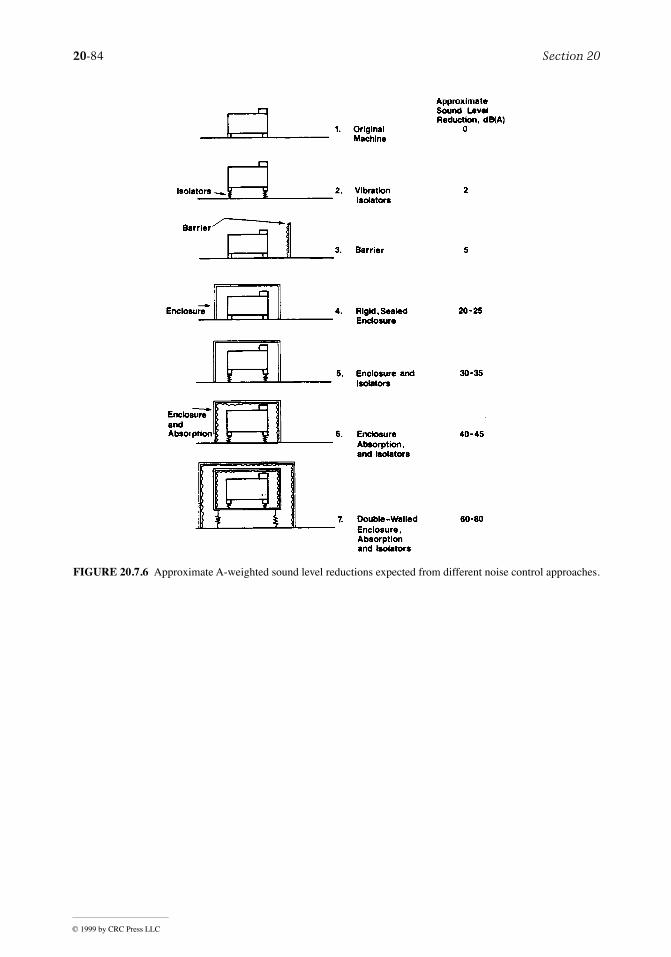
20-84 Section 20
© 1999 by CRC Press LLC
FIGURE 20.7.6 Approximate A-weighted sound level reductions expected from different noise control approaches.

Patent Law and Miscellaneous Topics 20-85
© 1999 by CRC Press LLC
20.8 Lighting Technology*
Barbara Atkinson, Andrea Denver, James E. McMahon, Leslie Shown, Robert Clear, and Craig B. Smith
In this section, we describe the general categories of lamps, ballasts, and Þxtures in use today. In addition,we brießy discuss several techniques for improving the energy-efÞciency of lighting systems.
Because the purpose of a lamp is to produce light, and not just radiated power, there is no directmeasure of lamp efÞciency. Instead, a lamp is rated in terms of its efÞcacy, which is the ratio of theamount of light emitted (lumens) to the power (watts) drawn by the lamp. The unit used to express lampefÞcacy is lumens per watt (LPW). The theoretical limit of efÞcacy is 683 LPW and would be producedby an ideal light source emitting monochromatic radiation with a wavelength of 555 nm. The lamps thatare currently on the market produce from a few percent to almost 25% of the maximum possible efÞcacy.**
The efÞcacies of various light sources are depicted in Figure 20.8.1. Lamps also differ in terms of theircost; size; color; lifetime; optical controllability; dimmability; lumen maintenance***; reliability; sim-plicity and convenience in use, maintenance, and disposal; and environmental effects (e.g., emission ofnoise, radio interference, and ultraviolet (UV) light).
* The contents of this section have been abstracted from Chapers 10 (Electrical Energy Management in Buildingsby Craig B. Smith) and 12B (Energy EfÞcient Lighting Technologies and Their Applications in the Commercial andResidential Sectors by Barbara Atkinson, Andrea Denver, James E. McMahon, Leslie Shown, and Robert Clear)published in the CRC Handbook of Energy EfÞciency, Frank Kreith and Ronald E. West, Eds., 1997.
** The efÞcacies of ßuorescent lamp/ballast combinations reported in this section are based on data compiled byOliver Morse from tests by the National Electrical Manufacturer's Association; all comparisons assume SP41 lamps.EfÞcacies of incandescent lamps are based on manufacturer catalogs. EfÞcacies of high-intensity discharge lampsare based on manufacturer catalogs and an assumed ballast factor of 0.95.
*** Over time, most lamps continue to draw the same amount of power but produce fewer lumens. The lumenmaintenance of a lamp refers to the extent to which the lamp sustains its lumen output, and therefore efÞcacy, overtime.
FIGURE 20.8.1 Ranges of lamp efÞcacy. (Ballast losses are included for all discharge lamps.) (Compiled fromU.S. DOE, 1993a; Morse, personal communication, 1994; and manufacturer's catalogs.)

20-86 Section 20
© 1999 by CRC Press LLC
The color properties of a lamp are described by its color temperature and its color rendering index.Color temperature, expressed in degrees Kelvin (K), is a measure of the color appearance of the lightof a lamp. The concept of color temperature is based on the fact that the emitted radiation spectrum ofa blackbody radiator depends on temperature alone. The color temperature of a lamp is the temperatureat which an ideal blackbody radiator would emit light that is closest in color to the light of the lamp.Lamps with low color temperatures (3000 K and below) emit ÒwarmÓ white light that appears yellowishor reddish in color. Incandescent and warm-white ßuorescent lamps have a low color temperature. Lampswith high color temperatures (3500 K and above) emit ÒcoolÓ white light that appears bluish in color.Cool-white ßuorescent lamps have a high color temperature.
The color rendering index (CRI) of a lamp is a measure of how surface colors appear whenilluminated by the lamp compared to how they appear when illuminated by a reference source of thesame color temperature. For color temperatures above 5000 K, the reference source is a standard daylightcondition of the same color temperature; below 5000 K, the reference source is a blackbody radiator.The CRI of a lamp indicates the difference in the perceived color of objects viewed under the lamp andunder the reference source. There are 14 differently colored test samples, 8 of which are used in thecalculation of the general CRI index.
The CRI is measured on a scale that has a maximum value of 100 and is an average of the resultsfor the 8 colors observed. A CRI of 100 indicates that there is no difference in perceived color for anyof the test objects; a lower value indicates that there are differences. CRIs of 70 and above are generallyconsidered to be good, while CRIs of 20 and below are considered to be quite poor. Most incandescentlamps have CRIs equal to or approaching 100. Low-pressure sodium lamps have the lowest CRI of anycommon lighting source (Ð44); their light is essentially monochromatic.
The optical controllability of a lamp describes the extent to which a user can direct the light of thelamp to the area where it is desired. Optical controllability depends on the size of the light-emittingarea, which determines the beam spread of the light emitted. In addition, controllability depends on theÞxture in which the lamp is used. Incandescent lamps emit light from a small Þlament area: they arealmost point sources of light, and their optical controllability is excellent. In contrast, ßuorescent lampsemit light from their entire phosphored area: their light is extremely diffuse, and their controllability ispoor.
Because of the many different characteristics and the variety of applications by which a lamp can bejudged, no one type of source dominates the lighting market. The types of lamps that are commonlyavailable include incandescent, ßuorescent, and high-intensity discharge (HID).
Lamps
The incandescent lamp was invented independently by Thomas Edison in the United States and JosephSwan in England in the late 1800s. An incandescent lamp produces light when electricity heats the lampÞlament to the point of incandescence. In modern lamps the Þlament is made of tungsten. Because 90%or more of an incandescent's emissions are in the infrared (thermal) rather than the visible range of theelectromagnetic spectrum, incandescent lamps are less efÞcacious than other types of lamps.
The two primary types of standard incandescent lamps are general service and reßector/PAR (parabolicaluminized reßector) lamps. General-service lamps (also known as A-lamps) are the pear-shaped, com-mon household lamps. Reßector lamps, such as ßood or spotlights, are generally used to illuminateoutdoor areas or highlight indoor retail displays and artwork. They are also commonly used to improvethe optical efÞciency of downlights (discussed later). Downlights are used where controlling glare orhiding the light source is important.
In spite of the fact that they are the least efÞcacious lamps on the market today, standard incandescentlamps are used for almost all residential lighting in the U.S. and are also common in the commercialsector. They have excellent CRIs and a warm color; they are easily dimmed, inexpensive, small,lightweight, and can be used with inexpensive Þxtures; and, in a properly designed Þxture, they permit
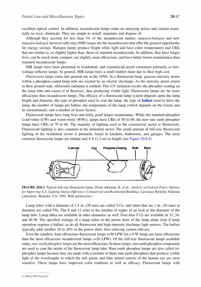
Patent Law and Miscellaneous Topics 20-87
© 1999 by CRC Press LLC
excellent optical control. In addition, incandescent lamps make no annoying noises and contain essen-tially no toxic chemicals. They are simple to install, maintain, and dispose of.
Although they account for less than 3% of the incandescent market, tungsten-halogen and nowtungsten-halogen infrared-reßecting (HIR) lamps are the incandescents that offer the greatest opportunityfor energy savings. Halogen lamps produce bright white light and have color temperatures and CRIsthat are similar to, or slightly higher than, those of standard incandescents. In addition, they have longerlives, can be much more compact, are slightly more efÞcacious, and have better lumen maintenance thanstandard incandescent lamps.
HIR lamps have been promoted to residential- and commercial-sector customers primarily as low-wattage reßector lamps. In general, HIR lamps have a small market share due to their high cost.
Fluorescent lamps came into general use in the 1950s. In a ßuorescent lamp, gaseous mercury atomswithin a phosphor-coated lamp tube are excited by an electric discharge. As the mercury atoms returnto their ground state, ultraviolet radiation is emitted. This UV radiation excites the phosphor coating onthe lamp tube and causes it to ßouresce, thus producing visible light. Fluorescent lamps are far moreefÞcacious than incandescent lamps. The efÞcacy of a ßuorescent lamp system depends upon the lamplength and diameter, the type of phosphor used to coat the lamp, the type of ballast used to drive thelamp, the number of lamps per ballast, the temperature of the lamp (which depends on the Þxture andits environment), and a number of lesser factors.
Fluorescent lamps have long lives and fairly good lumen maintanance. While the standard-phosphor(cool-white (CW) and warm-white (WW)), lamps have CRIs of 50 to 60, the new rare earth phosphorlamps have CRIs of 70 to 80. The majority of lighting used in the commercial sector is ßuorescent.Fluorescent lighting is also common in the industrial sector. The small amount of full-size ßuorescentlighting in the residential sector is primarily found in kitchens, bathrooms, and garages. The mostcommon ßuorescent lamps are tubular and 4 ft (1.2 m) in length (see Figure 20.8.2).
Lamp tubes with a diameter of 1.5 in. (38 mm) are called T12s, and tubes that are 1 in. (26 mm) indiameter are called T8s. The 8 and 12 refer to the number of eights of an inch in the diameter of thelamp tube. Lamp tubes are available in other diameters as well. Four-foot T12s are available in 32, 34,and 40 W. The speciÞed wattage of a lamp refers to the power draw of the lamp alone even if lampoperation requires a ballast, as do all ßuorescent and high-intensity discharge light sources. The ballasttypically adds another 10 to 20% to the power draw, thus reducing system efÞcacy.
Even the smallest, least efÞcacious ßuorescent lamps (»30 LPW for a 4-W lamp) are more efÞcaciousthan the most efÞcacious incandescent lamps (»20 LPW). Of the full-size ßuorescent lamps availabletoday, rare earth phosphor lamps are the most efÞcacious. In these lamps, rare earth phosphor compoundsare used to coat the inside of the ßuorescent lamp tube. Rare earth phosphor lamps are also called tri-phosphor lamps because they are made with a mixture of three rare earth phosphors that produce visiblelight of the wavelengths to which the red, green, and blue retinal sensors of the human eye are mostsensitive. These lamps have improved color rendition as well as efÞcacy. Fluorescent lamps with
FIGURE 20.8.2 Typical full-size ßuorescent lamp. (From Atkinson, B. et al., Analysis of Federal Policy Optionsfor Improving U.S. Lighting Energy EfÞciency: Commercial and Residential Buildings, Lawrence Berkeley NationalLaboratory, Berkeley, CA, 1992. With permission.)

20-88 Section 20
© 1999 by CRC Press LLC
diameters of 1 in. (26 mm) and smaller use tri-phosphors almost exclusively. Rare earth coatings canalso be used for lamps of larger diameter.
The most efÞcacious of the ßuorescent lamps available today are T8 lamps operating with electronicballasts. The efÞcacy of two 32-W T8 lamps operating with a single electronic ballast is about 90 LPW,approximately 30% more efÞcacious than the more standard lighting system consisting of two 40-WT12 lamps and a high-efÞciency magnetic ballast. T12 lamps are also available with rare earth phosphors,and can attain over 80 LPW when used with a two-lamp electronic ballast. The characteristics andapplications of 4-ft T8 lamps are summarized in Table 20.8.1.
In spite of their much greater efÞciency, ßuorescent lamps have several disadvantages when comparedto incandescent lamps. Fluorescent lamps can be dimmed, but only with special equipment that costsmuch more than the dimming controls used for incandescent lamps. Standard ßuorescent lamps aremuch bigger than incandescent lamps of equivalent output and are much harder to control optically. Inaddition, ßuorescent lamps contain trace amounts of mercury, a toxic metal, and emit more UV lightthan incandescent lamps. The ballast equipment that drives the lamps is sometimes noisy and may emitradio interference.
Circular ßuorescent lamps in 20- to 40-W sizes have been available for many years, but have alwayshad a fairly small market. Essentially, a circular lamp is a standard ßuorescent lamp tube (as describedearlier) that has been bent into a circle. Although they have a more compact geometry than a straighttube, circular lamps are still moderately large (16.5 to 41 cm in diameter).
Compact ßuorescent lamps (CFLs), which are substantially smaller than standard ßuorescent lamps,were introduced to the U.S. market in the early 1980s. In a CFL, the lamp tube is smaller in diameterand is bent into two to six sections (see Figure 20.8.3). CFLs have much higher power densities perphosphor area than standard ßuorescents, and their design was therefore dependent on the developmentof rare earth phosphors, which could hold up much better than standard phosphors at high power loadings.CFLs are available as both screw-in replacements for incandescent lamps and as pin-base lamps forhard-wired Þxtures. They may be operated with separate ballasts or purchased as integral lamp/ballastunits.
High-intensity discharge lamps produce light by discharging an electrical arc through a mixture ofgases. In contrast to ßuorescent lamps, HID lamps use a compact Òarc tubeÓ in which both temperatureand pressure are very high. Compared to a ßuorescent lamp, the arc tube in an HID lamp is small enoughto permit compact reßector designs with good light control. Consequently, HID lamps are both compactand powerful. There are currently three common types of HID lamps available: mercury vapor (MV),metal halide (MH), and high-pressure sodium (HPS).
TABLE 20.8.1 Characteristics and Applications of 4-ft Full-Size Fluorescent T8 Lamps
Available wattages 32 WEfÞcacy For two T8s and a single electronic ballast, »90 LPWRated lifetime Typically 12,000 to 20,000 hrColor rendition Typically 75Ð84Color temperature 2800Ð7500 KLumen maintenance Very good (light output typically declines by 10 to 12% over rated lamp life)Optical controllability Poor (very diffuse light but slightly better than a T12)Typical uses The majority of lighting used in the commercial sector is ßuorescent.
Fluorescent lighting is also used in the industrial sector. In the residential sector, full-size ßuorescent lighting is used in some kitchens, bathrooms, and garages
Technologies for which these lamps are energy-efÞcient alternatives
These lamps are most often replacements for less-efÞcient ßuorescents (T12s)
Notes Some T8 lamps are now available with CRIs above 90, especially those with high color temperature; however, these lamps are less efÞcacious than lamps with lower CRIs

Patent Law and Miscellaneous Topics 20-89
© 1999 by CRC Press LLC
Because of their very high light levels, except in the smallest lamps, and their substantial cost ($15to 80 for lamps up to 400 W), HID lamps are most often used for exterior applications such as streetlighting and commercial, industrial, and residential ßoodlighting (sports and security lighting). They arealso used in large, high-ceilinged, interior spaces such as industrial facilitites and warehouses, wheregood color is not typically a priority. Occasionally, HID lamps are used for indirect lighting in commercialofÞces. Interior residential applications are rare because of high cost, high light level, and the fact thatHID lamps take several minutes to warm up to full light output. If there is a momentary power outage,the lamps must cool down before they will restrike. Some HID lamps are now available with dual arctubes or parallel Þlaments. Dual arc tubes eliminate the restrike problem and a parallel Þlament givesinstantaneous light output both initially and on restrike, but at a cost of a high initial power draw.
The mercury vapor lamp was the Þrst HID lamp developed. Including ballast losses, the efÞcacies ofMV lamps range from about 25 to 50 LPW. Uncoated lamps have a bluish tint and very poor colorrendering (CRI » 15). Phosphor-coated lamps emit more red, but are still bluish, and have a CRI ofabout 50. Because of their poor color rendition, these lamps are only used where good color is not apriority. Although MV lamps generally have rated lifetimes in excess of 24,000 hr, light output candiminish signiÞcantly after only 12,000 hr (Audin et al., 1994). Both metal halide and high-pressuresodium HIDD lamps have higher efÞcacies than mercury vapor lamps and have consequently replacedthem in most markets.
Including ballast losses, metal halide lamps range in efÞcacy from 46 to 100 LPW. They produce awhite to slightly bluish-white light and have CRIs ranging from 65 to 70. Lamp lifetimes range fromonly 3500 to 20,000 hr, depending on the type of MH lamp. Lower-wattage metal halides (particularlythe 70-W and 100-W) are now available with CRIs of 65 to 75 and color temperatures of 3200 to 4200K. Good lumen maintenance, longer life, reduced maintenance costs, and the fact that they blend morenaturally with ßuorescent sources have made MH lamps a very good replacement in the commercialsector for 300-W and 500-W PAR lamps. New Þxtures utilizing these lamps, particularly 1-ft by 1-ftrecessed lensed troffers (downlights), are becoming common in lobbies, shopping malls, and retail stores.
Including ballast losses, high-pressure sodium lamps have efÞcacies ranging from 50 LPW for thesmallest lamps to 124 LPW for the largest lamps. Standard HPS lamps emit a yellow light and havevery poor color rendition. Like MV lamps, HPS lamps are only used where good color is not a priority.The rated lifetimes of HPS lamps rival those of MV lamps and typically exceed 24,000 hr.
FIGURE 20.8.3 A variety of compact ßuorescent and circular lamps: (a) twin-tube integral, (b and c) triple-tubeintegrals, (d) integral model with glare-reducing casing, (e) modular quad tube and ballast, and (f) modular circlineand ballast. (Courtesy of Katherine Falk and Home Energy magazine, 1995.)

20-90 Section 20
© 1999 by CRC Press LLC
Ballasts
Because both ßuorescent and HID lamps (discharge lamps) have a low resistance to the ßow of electriccurrent once the discharge arc is struck, they require some type of device to limit current ßow. A lampballast is an electrical device used to control the current provided to the lamp. In most discharge lamps,a ballast also provides the high voltage necessary to start the lamp. Older ÒpreheatÓ ßuorescent lampsrequire a separate starter, but these lamps are becoming increasingly uncommon. In many HID ballasts,the ignitor used for starting the lamp is a replaceable module.
The most common types of ballasts are magnetic core-coil and electronic high-frequency ballasts. Amagnetic core-coil ballast uses a transformer with a magnetic core coiled in copper or aluminum wireto control the current provided to a lamp. Magnetic ballasts operate at an input frequency of 60 Hz andoperate lamps at the same 60 Hz. An electronic high-frequency ballast uses electronic circuitry ratherthan magnetic components to control current. Electronic ballasts use standard 60 Hz power but operatelamps at a much higher frequency (20,000 to 60,000 Hz). Both magnetic and electronic ballasts areavailable for most ßuorescent lamp types.
Of the ballasts that are currently available for ßuorescent lamps, the most efÞcient options are theelectronic ballast and the cathode cutout ballast. Because an electronic ballast is more efÞcient than astandard core-coil magnetic ballast in transforming the input power to lamp requirements, and becauseßuorescent lamps are more efÞcient when operated at frequencies of 20,000 Hz or more, a lamp/ballastsystem using an electronic rather than magnetic ballast is more efÞcacious. Where there are two lampsper ballast, electronic ballast systems are approximately 20% more efÞcacious than magnetic ballastsystems; where there is only one lamp per ballast, electronic ballast systems are almost 40% moreefÞcacious than magnetic ballast systems.
In addition, electronic ballasts eliminate ßicker, weigh less than magnetic ballasts, and operate morequietly. Since electronic ballasts are packaged in ÒcansÓ that are the same size as magnetic ballasts, theycan be placed in Þxtures designed to be used with magnetic ballasts. Electronic ballasts are widelyavailable, but their use is limited because of their high cost and some technological limitations for certainapplications. Fluorescent electronic ballasts are available for standard commercial-sector applications.
The cathode cut-out (hybrid) ballast is a modiÞed magnetic ballast. It uses an electronic circuit toremove the Þlament power after the discharge has been initiated for rapid-start lamps. Cathode cut-outballasts use approximately 5 to 10% less energy than energy-efÞcient magnetic ballasts. Almost allballasts used for HID lamps are magnetic, and a number of different types are available. The varioustypes differ primarily in how well they tolerate voltage swings and, in the case of HPS lamps, theincreased voltage required to operate the lamp as it ages.
Lighting Fixtures
A lighting Þxture is a housing for securing lamp(s) and ballast(s) and for controlling light distributionto a speciÞc area. The function of the Þxture is to distribute light to the desired area without causingglare or discomfort. The distribution of light is determined by the geometric design of the Þxture as wellas the material of which the reßector and/or lens is made. The more efÞcient a Þxture is, the more lightit emits from the lamp(s) within it. Although a lighting Þxture is sometimes referred to as a luminaire,the term luminaire is most commonly used to refer to a complete lighting system including a lamp,ballast, and Þxture.
Types of ßuorescent lighting Þxtures that are commonly used in the nonresidential sectors includerecessed troffers, pendant-mounted indirect Þxtures and indirect/direct Þxtures, and surface-mountedcommercial Þxtures such as wraparound, strip, and industrial Þxtures.
Most ofÞces are equipped with recessed troffers, which are direct (downward) Þxtures and emphasizehorizontal surfaces. Many forms of optical control are possible with recessed luminaires. In the past,prismatic lenses were the preferred optical control because they offer high luminaire efÞciency anduniform illuminance in the work space. Electronic ofÞces have become increasingly common, however,

Patent Law and Miscellaneous Topics 20-91
© 1999 by CRC Press LLC
and the traditional direct lighting Þxtures designed for typing and other horizontal tasks have becomeless useful because they tend to cause reßections on video display terminal (VDT) screens.
No lighting system reduces glare entirely, but some Þxtures and/or components can reduce the amountof glare signiÞcantly. Because the glossy, vertical VDT screen can potentially reßect bright spots on theceiling, and because VDT work is usually done with the head up, existing Þxtures are sometimes replacedwith indirect or direct/indirect Þxtures, which produce light that is considered more visually comfortable.Most indirect lighting systems are suspended from the ceiling. They direct light toward the ceiling wherethe light is then reßected downward to provide a calm, diffuse light. Some people describe the indirectlighting as similar to the light on an overcast day, with no shadows or highlights. Generally, indirectlighting does not cause bright reßections on VDT screens. A direct/indirect Þxture is suspended fromthe ceiling and provides direct light as well as indirect. These Þxtures combine the high efÞciency ofdirect lighting systems with the uniformity of light and lack of glare produced by indirect lightingsystems.
A wraparound Þxture has a prismatic lens that wraps around the bottom and sides of the lamp, andis always surface mounted rather than recessed. Wraparound Þxtures are less expensive than othercommercial Þxtures and are typically used in areas where lighting control and distribution are not apriority. Strip and industrial Þxtures are even less expensive and are typically used in places where lightdistribution is less important, such as large open areas (grocery stores, for example) and hallways. Theseare open Þxtures in which the lamp is not hidden from view. The most common incandescent Þxture inthe nonresidential sector is the downlight, also known as a recessed can Þxture. Fixtures designed forCFLs are available to replace downlight Þxtures in areas where lighting control is less critical.
Lighting Efficiency*
There are seven techniques for improving the efÞciency of lighting systems:
¥ Delamping
¥ Relamping
¥ Improved controls
¥ More efÞcient lamps and devices
¥ Task-oriented lighting
¥ Increased use of daylight
¥ Room color changes, lamp maintenance
The Þrst two techniques and possibly the third are low in cost and may be considered operational changes.The last four items generally involve retroÞt or new designs.
The Þrst step in reviewing lighting electricity use is to perform a lighting survey. An inexpensivehand-held light meter can be used as a Þrst approximation; however, distinction must be made betweenraw intensities (lux or footcandles) recorded in this way and equivalent sphere illumination (ESI) values.
Many variables can affect the ÒcorrectÓ lighting values for a particular task: task complexity, age ofemployee, glare, and so on. For reliable results, consult a lighting specialist or refer to the literature andpublications of the Illuminating Engineering Society.
The lighting survey indicates those areas of the building where lighting is potentially inadequate orexcessive. Deviations from adequate illumination levels can occur for several reasons: overdesign,building changes, change of occupancy, modiÞed layout of equipment or personnel, more efÞcient lamps,
* It should be noted that the ÒLighting EfÞciencyÓ discussion was written by a different author than the earliermaterial in the chapter, and that there are some discrepancies between the lamp efÞcacy ranges reported in the twosections. These discrepancies are likely the result of the different data sources used to calculate efÞcacy ranges, thedifferent time periods during which they were calculated, and different assumptions regarding which lamp types aremost typical.

20-92 Section 20
© 1999 by CRC Press LLC
improper use of equipment, dirt buildup, and so on. Once the building manager has identiÞed areas withpotentially excessive illumination levels, he or she can apply one or more of the seven techniques listedearlier. Each of these will be described brießy.
Delamping refers to the removal of lamps to reduce illumination to acceptable levels. With incandes-cent lamps, bulbs are removed. With ßuorescent or HID lamps, ballasts account for 10 to 20% of totalenergy use and should be disconnected after lamps are removed.
Fluorescent lamps often are installed in luminaires in groups of two or more lamps where it isimpossible to remove only one lamp. In such cases an artiÞcial load (called a Òphantom tubeÓ) can beinstalled in place of the lamp that has been removed.
Relamping refers to the replacement of existing lamps by lamps of lower wattage or increasedefÞciency. Low-wattage ßuorescent tubes are available that require 15 to 20% less wattage (but produce
10 to 15% less light). In some types of HID lamps, a more efÞcient lamp can be substituted directly.However, in most cases, ballasts must also be changed. Table 20.8.2 shows typical savings by relamping.
Improved controls permit lamps to be used only when and where needed. For example, certain ofÞcebuildings have all lights for one ßoor on a single contactor. These lamps will be switched on at 6 A.M.,before work begins, and are not turned off until 10 P.M., when maintenance personnel Þnish their cleanupduties. Energy usage can be cut by as much as 50% by installing individual switches for each ofÞce orwork area, installing time clocks, installing occupancy sensors, using photocell controls, or instructingcustodial crews to turn lights on as needed and turn them off when work is complete.
There is a great variation in the efÞcacy (a measure of light output per electricity input) of variouslamps. Since incandescent lamps have the lowest efÞcacy, typically 8 to 20 LPW, wherever possible,ßuorescent lamps should be substituted. This not only saves energy but also offers economic savings,since ßuorescent lamps last 10 to 50 times longer. Fluorescent lamps have efÞcacies in the range of 30to 90 LPW.
Compact ßuorescent lamps are available as substitutes for a wide range of incandescent lamps. Theyrange in wattage from 5 to 25 W with efÞcacies of 26 to 58 lm/W and will replace 25- to 100-Wincandescent lamps. In addition to the energy savings, they have a 10,000-hr rated life and do not needto be replaced as often as incandescent lamps. Exit lights are good candidates for compact ßuorescentlamps. Conversion kits are available to replace the incandescent lamps. Payback is rapid because of thelower energy use and lower maintenance cost, since these lamps are normally on 24 hr a day. There arealso light-emitting diode exit lights that are very energy efÞcient.
TABLE 20.8.2 Typical Relamping Opportunities
Change OfÞce Lamps(2700 hr per year)
Energy Savings/Cost Savings
kWh GJe 5¢ kWhFrom To To save annually
1 300-W incandescent 1 100-W mercury vapor 486 5.25 $24.302 100-W incandescent 1 40-W ßuorescent 400 4.32 20.007 150-W incandescent 1 150-W sodium vapor 2360 25.5 $118.00Change industrial lamps (3000 hr per year)
1 300-W incandescent 2 40-W ßuorescent 623 6.73 $31.151 100-W incandescent 2 215-W ßuorescent 1617 17.5 80.853 300-W incandescent 1 250-W sodium vapor 1806 19.5 90.30Change store lamps(3300 hr per year)
1 300-W incandescent 2 40-W ßuorescent 685 7.40 $34.251 200-W incandescent 1 100-W mercury vapor 264 2.85 13.202 200-W incandescent 1 175-W mercury vapor 670 7.24 33.50
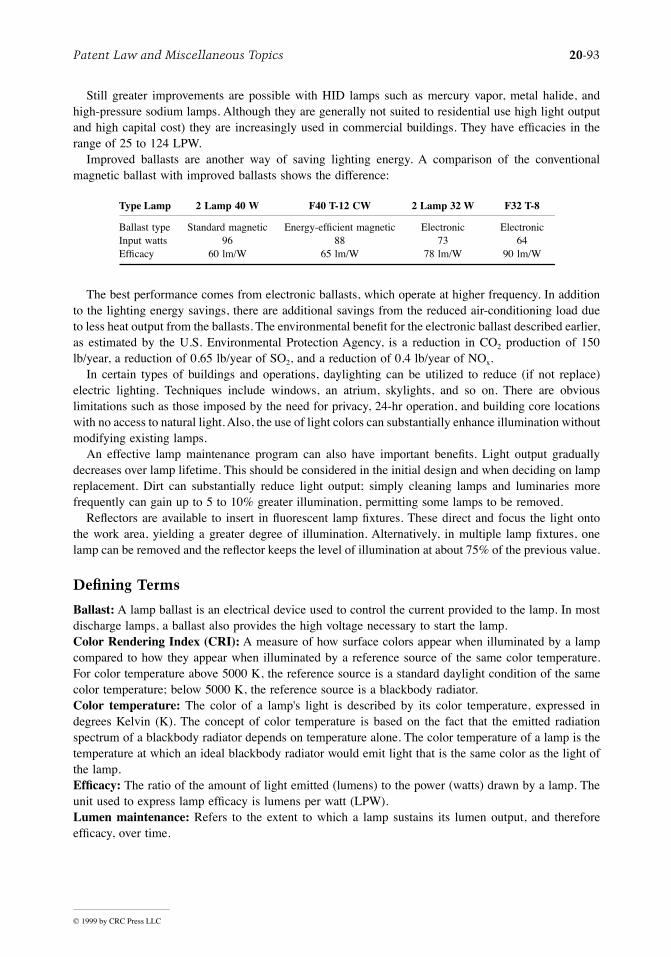
Patent Law and Miscellaneous Topics 20-93
© 1999 by CRC Press LLC
Still greater improvements are possible with HID lamps such as mercury vapor, metal halide, andhigh-pressure sodium lamps. Although they are generally not suited to residential use high light outputand high capital cost) they are increasingly used in commercial buildings. They have efÞcacies in therange of 25 to 124 LPW.
Improved ballasts are another way of saving lighting energy. A comparison of the conventionalmagnetic ballast with improved ballasts shows the difference:
The best performance comes from electronic ballasts, which operate at higher frequency. In additionto the lighting energy savings, there are additional savings from the reduced air-conditioning load dueto less heat output from the ballasts. The environmental beneÞt for the electronic ballast described earlier,as estimated by the U.S. Environmental Protection Agency, is a reduction in CO2 production of 150lb/year, a reduction of 0.65 lb/year of SO2, and a reduction of 0.4 lb/year of NOx.
In certain types of buildings and operations, daylighting can be utilized to reduce (if not replace)electric lighting. Techniques include windows, an atrium, skylights, and so on. There are obviouslimitations such as those imposed by the need for privacy, 24-hr operation, and building core locationswith no access to natural light. Also, the use of light colors can substantially enhance illumination withoutmodifying existing lamps.
An effective lamp maintenance program can also have important beneÞts. Light output graduallydecreases over lamp lifetime. This should be considered in the initial design and when deciding on lampreplacement. Dirt can substantially reduce light output; simply cleaning lamps and luminaries morefrequently can gain up to 5 to 10% greater illumination, permitting some lamps to be removed.
Reßectors are available to insert in ßuorescent lamp Þxtures. These direct and focus the light ontothe work area, yielding a greater degree of illumination. Alternatively, in multiple lamp Þxtures, onelamp can be removed and the reßector keeps the level of illumination at about 75% of the previous value.
Defining Terms
Ballast: A lamp ballast is an electrical device used to control the current provided to the lamp. In mostdischarge lamps, a ballast also provides the high voltage necessary to start the lamp.Color Rendering Index (CRI): A measure of how surface colors appear when illuminated by a lampcompared to how they appear when illuminated by a reference source of the same color temperature.For color temperature above 5000 K, the reference source is a standard daylight condition of the samecolor temperature; below 5000 K, the reference source is a blackbody radiator.Color temperature: The color of a lamp's light is described by its color temperature, expressed indegrees Kelvin (K). The concept of color temperature is based on the fact that the emitted radiationspectrum of a blackbody radiator depends on temperature alone. The color temperature of a lamp is thetemperature at which an ideal blackbody radiator would emit light that is the same color as the light ofthe lamp.EfÞcacy: The ratio of the amount of light emitted (lumens) to the power (watts) drawn by a lamp. Theunit used to express lamp efÞcacy is lumens per watt (LPW).Lumen maintenance: Refers to the extent to which a lamp sustains its lumen output, and thereforeefÞcacy, over time.
Type Lamp 2 Lamp 40 W F40 T-12 CW 2 Lamp 32 W F32 T-8
Ballast type Standard magnetic Energy-efÞcient magnetic Electronic ElectronicInput watts 96 88 73 64EfÞcacy 60 lm/W 65 lm/W 78 lm/W 90 lm/W

20-94 Section 20
© 1999 by CRC Press LLC
References
Atkinson, B., McMahon, J., Mills, E., Chan, P., Chan, T., Eto, J., Jennings, J., Koomey, J., Lo, K., Lecar,M., Price, L., Rubinstein, F., Sezgen, O., and Wenzel, T. 1992. Analysis of Federal Policy Optionsfor Improving U.S. Lighting Energy EfÞciency: Commercial and Residential Buildings. LawrenceBerkeley National Laboratory, Berkeley, CA. LBL-31469.
Audin, L., Houghton, D., Shepard, M., and Hawthorne, W. 1994. Lighting Technology Atlas. E-Source,Snowmass, CO.
Illuminating Engineering Society of North Amercia. 1993. Lighting Handbook, 8th ed., M. Rhea, Ed.,Illuminating Engineering Society of North America, New York.
Leslie, R. and Conway, K. 1993. The Lighting Pattern Book for Homes, Lighting Research Center,Rensselaer Polytechnic Institute, Troy, NY.
Turiel, I., Atkinson, B., Boghosian, S., Chan, P., Jennings, J., Lutz, J., McMahon, J., and Roenquist, G.1995. Evaluation of Advanced Technologies for Residential Appliances and Residential and Com-mercial Lighting. Lawrence Berkely National Laboratory, Berkeley, CA. LBL-35982.
Further Information
For additional information on performance characteristics of lamps, ballasts, lighting Þxtures, andcontrols, the reader is referred to the CRC Handbook of Energy EfÞciency from which this section hasbeen extracted. If interested in more discussions of energy-efÞcient lighting design strategies andtechnologies, consult the references and request information from the Green Lights program: GreenLights U.S. EPA, Air and Radiation (6202-J), Washington, D.C., 20460.

Norton, P. “Appendices”Mechanical Engineering HandbookEd. Frank KreithBoca Raton: CRC Press LLC, 1999
c©1999 by CRC Press LLC

A
-1
© 1999 by CRC Press LLC
Appendices
A. Properties of Gases and Vapors ...........................................A-2B. Properties of Liquids.......................................................... B-35C. Properties of Solids ............................................................ C-38D. SI Units ..............................................................................D-74E. Miscellaneous ..................................................................... E-75
Paul Norton
National Renewable Energy Laboratory

A
-2
Appendix A
© 1999 by CRC Press LLC
Appendix A. Properties of Gases and Vapors
TABLE A.1 Properties of Dry Air at Atmospheric Pressure
Symbols and Units:
K =
absolute temperature, degrees Kelvindeg
C
= temperature, degrees Celsiusdeg
F
= temperature, degrees Fahrenheit
r
= density, kg/m
3
c
p
= speciÞc heat capacity, kJ/kgáKc
p
/c
v
= speciÞc heat capacity ratio, dimensionless
m
= viscosity, Nás/m
2
´
10
6
(For Nás/m
2
(= kg/más) multiply tabulated values by 10
Ð6
)
k
= thermal conductivity, W/mák
´
10
3
(For W/máK multiply tabulated values by 10
Ð3
)
Pr
= Prandtl number, dimensionless
h
= enthalpy, kJ/kg
V
s
= sound velocity, m/s
AAppendix A
Gases and Vapors

Gases and Vapors
A
-3
© 1999 by CRC Press LLC
TABLE A.1 (continued) Properties of Dry Air at Atmospheric Pressure

A
-4
Appendix A
© 1999 by CRC Press LLC
TABLE A.2 Ideal Gas Properties of Nitrogen, Oxygen, and Carbon Dioxide
Symbols and Units:
T
= absolute temperature, degrees Kelvin= enthalpy, kJ/kmol= internal energy, kJ/kmol= absolute entropy at standard reference pressure, kJ/kmol K= enthalpy of formation per mole at standard state = 0 kJ/kmol]
Part a. Ideal Gas Properties of Nitrogen, N
2
Source:
Adapted from M.J. Moran and H.N. Shapiro,
Fundamentals of Engineering Thermodynamics
, 3rd. ed., Wiley, New York, 1995, as presented in K. Wark.
Thermodynamics
, 4th ed., McGraw-Hill, New York, 1983, based on the
JANAF Thermochemical Tables
, NSRDS-NBS-37, 1971.
hus°[h

Gases and Vapors
A
-5
© 1999 by CRC Press LLC
TABLE A.2 (continued) Ideal Gas Properties of Nitrogen, Oxygen, and Carbon Dioxide

A
-6
Appendix A
© 1999 by CRC Press LLC
Part b. Ideal Gas Properties of Oxygen, O
2
TABLE A.2 (continued) Ideal Gas Properties of Nitrogen, Oxygen, and Carbon Dioxide

Gases and Vapors
A
-7
© 1999 by CRC Press LLC
TABLE A.2 (continued) Ideal Gas Properties of Nitrogen, Oxygen, and Carbon Dioxide

A
-8
Appendix A
© 1999 by CRC Press LLC
Part c. Ideal Gas Properties of Carbon Dioxide, CO
2
TABLE A.2 (continued) Ideal Gas Properties of Nitrogen, Oxygen, and Carbon Dioxide

Gases and Vapors
A
-9
© 1999 by CRC Press LLC
TABLE A.2 (continued) Ideal Gas Properties of Nitrogen, Oxygen, and Carbon Dioxide
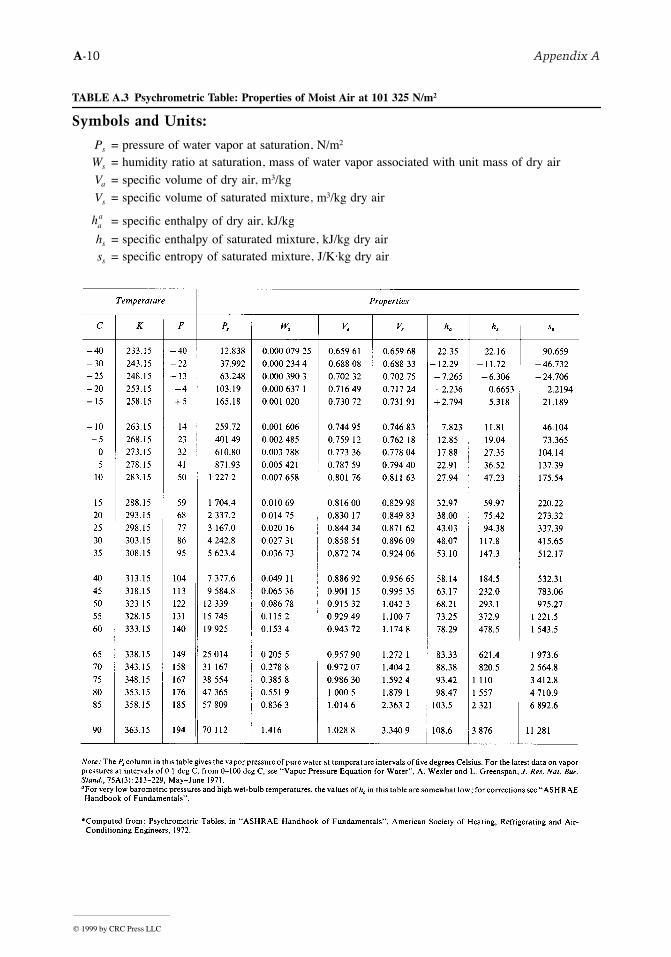
A
-10
Appendix A
© 1999 by CRC Press LLC
TABLE A.3 Psychrometric Table: Properties of Moist Air at 101 325 N/m
2
Symbols and Units:
P
s
= pressure of water vapor at saturation, N/m
2
W
s
= humidity ratio at saturation, mass of water vapor associated with unit mass of dry air
V
a
= speciÞc volume of dry air, m
3
/kg
V
s
= speciÞc volume of saturated mixture, m
3
/kg dry air
= speciÞc enthalpy of dry air, kJ/kg
h
s
= speciÞc enthalpy of saturated mixture, kJ/kg dry air
s
s
= speciÞc entropy of saturated mixture, J/Kákg dry air
haa
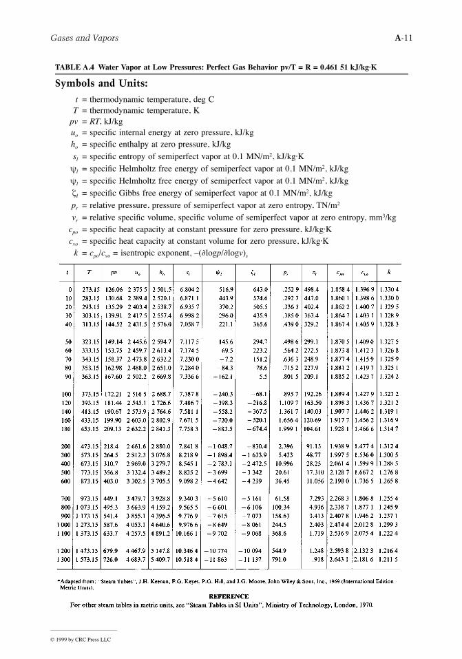
Gases and Vapors
A
-11
© 1999 by CRC Press LLC
TABLE A.4 Water Vapor at Low Pressures: Perfect Gas Behavior pv/T = R = 0.461 51 kJ/kgáK
Symbols and Units:
t
= thermodynamic temperature, deg C
T
= thermodynamic temperature, K
pv
=
RT
, kJ/kg
u
o
= speciÞc internal energy at zero pressure, kJ/kg
h
o
= speciÞc enthalpy at zero pressure, kJ/kg
s
l
= speciÞc entropy of semiperfect vapor at 0.1 MN/m
2
, kJ/kgáK
y
l
= speciÞc Helmholtz free energy of semiperfect vapor at 0.1 MN/m
2
, kJ/kg
y
l
= speciÞc Helmholtz free energy of semiperfect vapor at 0.1 MN/m
2
, kJ/kg
z
l
= speciÞc Gibbs free energy of semiperfect vapor at 0.1 MN/m
2
, kJ/kg
p
r
= relative pressure, pressure of semiperfect vapor at zero entropy, TN/m
2
v
r
= relative speciÞc volume, speciÞc volume of semiperfect vapor at zero entropy, mm
3
/kg
c
po
= speciÞc heat capacity at constant pressure for zero pressure, kJ/kgáK
c
vo
= speciÞc heat capacity at constant volume for zero pressure, kJ/kgáK
k
=
c
po
/
c
vo
= isentropic exponent, Ð(
log
p
/
log
v
)
s

A
-12
Appendix A
© 1999 by CRC Press LLC
TABLE A.5 Properties of Saturated Water and Steam
Part a. Temperature Table
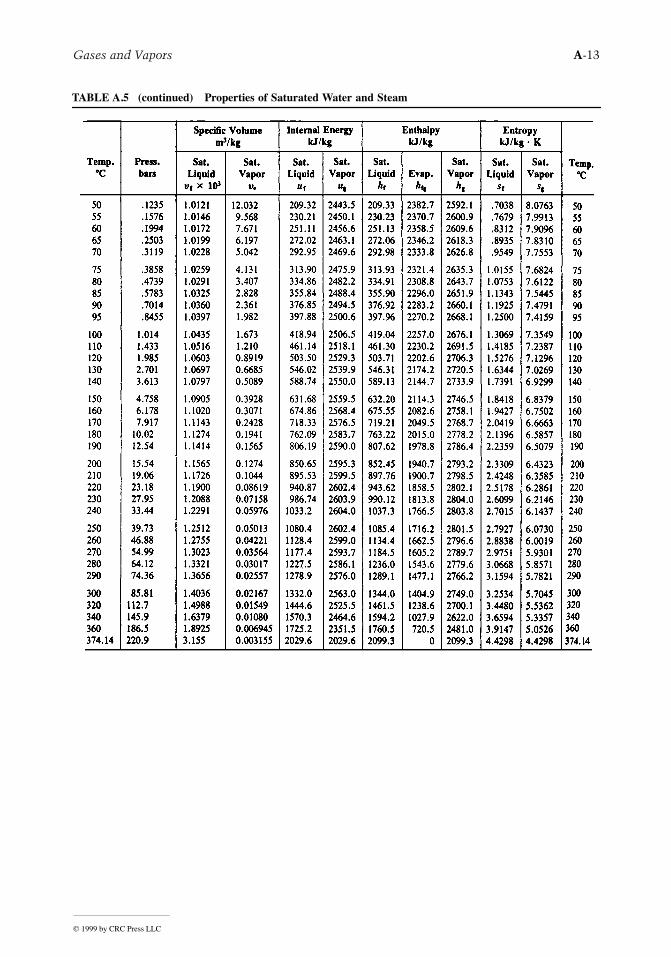
Gases and Vapors
A
-13
© 1999 by CRC Press LLC
TABLE A.5 (continued) Properties of Saturated Water and Steam

A
-14
Appendix A
© 1999 by CRC Press LLC
Part b. Pressure Table
Source:
Adapted from M.J. Moran and H.N. Shapiro,
Fundamentals of Engineering Thermodynamics
, 3rd. ed., Wiley, New York, 1995, as extracted from J.H. Keenan, F.G. Keyes, P.G. Hill, and J.G. Moore,
Steam Tables
, Wiley, New York, 1969.
TABLE A.5 (continued) Properties of Saturated Water and Steam
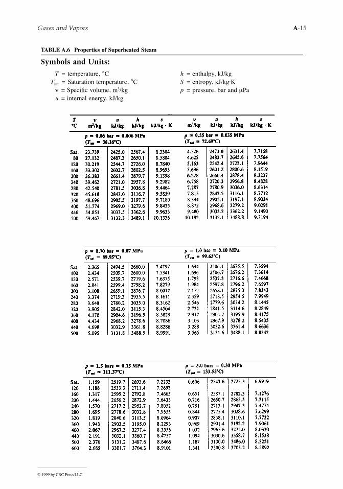
Gases and Vapors
A
-15
© 1999 by CRC Press LLC
TABLE A.6 Properties of Superheated Steam
Symbols and Units:
T =
temperature,
°
C
h
= enthalpy, kJ/kg
T
sat
=
Saturation temperature,
°
C
S
= entropy, kJ/kgáK
n
= SpeciÞc volume, m
3
/kg
p
= pressure, bar and
mPau = internal energy, kJ/kg

A-16 Appendix A
© 1999 by CRC Press LLC
TABLE A.6 (continued) Properties of Superheated Steam
Symbols and Units:
T = temperature, °C h = enthalpy, kJ/kgTsat = Saturation temperature, °C S = entropy, kJ/kgáK
n = SpeciÞc volume, m3/kg p = pressure, bar and mPau = internal energy, kJ/kg
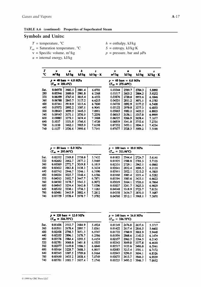
Gases and Vapors A-17
© 1999 by CRC Press LLC
TABLE A.6 (continued) Properties of Superheated Steam
Symbols and Units:
T = temperature, °C h = enthalpy, kJ/kgTsat = Saturation temperature, °C S = entropy, kJ/kgáK
n = SpeciÞc volume, m3/kg p = pressure, bar and mPau = internal energy, kJ/kg

A-18 Appendix A
© 1999 by CRC Press LLC
TABLE A.7 Chemical, Physical, and Thermal Properties of Gases: Gases and Vapors, Including Fuels and Refrigerants, English and Metric Units
Note: The properties of pure gases are given at 25°C (77°F, 298 K) and atmospheric pressure (except as stated).

Gases and Vapors A-19
© 1999 by CRC Press LLC
TABLE A.7 (continued) Chemical, Physical, and Thermal Properties of Gases: Gases and Vapors, Including Fuels and Refrigerants, English and Metric Units

A-20 Appendix A
© 1999 by CRC Press LLC
TABLE A.7 (continued) Chemical, Physical, and Thermal Properties of Gases: Gases and Vapors, Including Fuels and Refrigerants, English and Metric Units

Gases and Vapors A-21
© 1999 by CRC Press LLC
TABLE A.7 (continued) Chemical, Physical, and Thermal Properties of Gases: Gases and Vapors, Including Fuels and Refrigerants, English and Metric Units

A-22 Appendix A
© 1999 by CRC Press LLC
TABLE A.7 (continued) Chemical, Physical, and Thermal Properties of Gases: Gases and Vapors, Including Fuels and Refrigerants, English and Metric Units

Gases and Vapors A-23
© 1999 by CRC Press LLC
TABLE A.7 (continued) Chemical, Physical, and Thermal Properties of Gases: Gases and Vapors, Including Fuels and Refrigerants, English and Metric Units

A-24 Appendix A
© 1999 by CRC Press LLC
TABLE A.7 (continued) Chemical, Physical, and Thermal Properties of Gases: Gases and Vapors, Including Fuels and Refrigerants, English and Metric Units

Gases and Vapors A-25
© 1999 by CRC Press LLC
TABLE A.7 (continued) Chemical, Physical, and Thermal Properties of Gases: Gases and Vapors, Including Fuels and Refrigerants, English and Metric Units

A-26 Appendix A
© 1999 by CRC Press LLC
TABLE A.7 (continued) Chemical, Physical, and Thermal Properties of Gases: Gases and Vapors, Including Fuels and Refrigerants, English and Metric Units

Gases and Vapors A-27
© 1999 by CRC Press LLC
TABLE A.7 (continued) Chemical, Physical, and Thermal Properties of Gases: Gases and Vapors, Including Fuels and Refrigerants, English and Metric Units

A-28 Appendix A
© 1999 by CRC Press LLC
TABLE A.7 (continued) Chemical, Physical, and Thermal Properties of Gases: Gases and Vapors, Including Fuels and Refrigerants, English and Metric Units

Gases and Vapors A-29
© 1999 by CRC Press LLC
TABLE A.7 (continued) Chemical, Physical, and Thermal Properties of Gases: Gases and Vapors, Including Fuels and Refrigerants, English and Metric Units

A-30 Appendix A
© 1999 by CRC Press LLC
TABLE A.8 Ideal Gas Properties of Air
Part a. SI Units

Gases and Vapors A-31
© 1999 by CRC Press LLC
TABLE A.8 (continued) Ideal Gas Properties of Air

A-32 Appendix A
© 1999 by CRC Press LLC
TABLE A.8 (continued) Ideal Gas Properties of Air
Part b. English Units

Gases and Vapors A-33
© 1999 by CRC Press LLC
Source: Adapted from M.J. Moran and H.N. Shapiro, Fundamentals of Engineering Thermodynamics, 3rd. ed., Wiley, New York, 1995, as based on J.H. Keenan and J. Kaye, Gas Tables, Wiley, New York, 1945.
TABLE A.8 (continued) Ideal Gas Properties of Air

A-34
Appen
dix A
© 1999 by CRC Press LLC
TABLE A.9 Equations for Gas Properties
Source: Adapted from J.B. Jones and R.E. Dugan, Engineering Thermodynamics, Prentice-Hall, Englewood Cliffs, NJ 1996 from various sources: JANAF Thermochemical Tables, 3rd ed., published by the American Chemical Society and the American Institute of Physics for the National Bureau of Standards, 1986. Data for butane, ethane, and propane from K.A. Kobe and E.G. Long, ÒThermochemistry for the Petrochemical Industry, Part II Ñ ParafÞnic Hydrocarbons, C1ÐC16Ó Petroleum ReÞner, Vol. 28, No. 2, 1949, pp. 113Ð116.
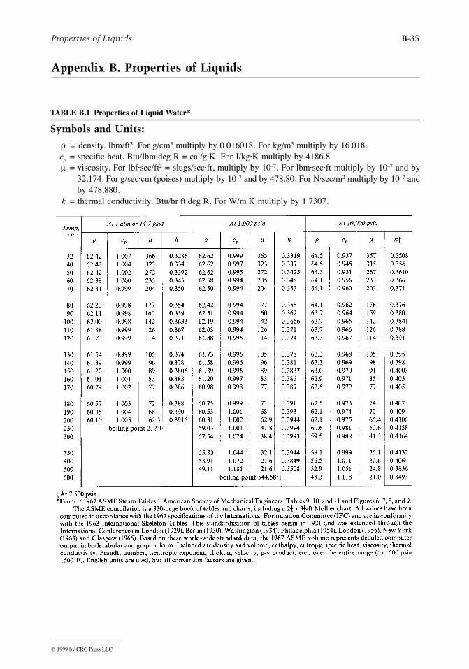
Properties of Liquids B-35
© 1999 by CRC Press LLC
Appendix B. Properties of Liquids
TABLE B.1 Properties of Liquid Water*
Symbols and Units:
r = density, lbm/ft3. For g/cm3 multiply by 0.016018. For kg/m3 multiply by 16.018.cp = speciÞc heat, Btu/lbmádeg R = cal/gáK. For J/kgáK multiply by 4186.8m = viscosity. For lbfásec/ft2 = slugs/secáft, multiply by 10Ð7. For lbmásecáft multiply by 10Ð7 and by
32.174. For g/secácm (poises) multiply by 10Ð7 and by 478.80. For Násec/m2 multiply by 10Ð7 andby 478.880.
k = thermal conductivity, Btu/hráftádeg R. For W/máK multiply by 1.7307.
BAppendix B
Properties of Liquids

B-36 Appendix B
© 1999 by CRC Press LLC
TABLE B.2 Physical and Thermal Properties of Common Liquids
Part a. SI Units(At 1.0 Atm Pressure (0.101 325 MN/m2), 300 K, except as noted.)

Properties of Liquids B-37
© 1999 by CRC Press LLC
TABLE B.2 (continued) Physical and Thermal Properties of Common Liquids
Part b. English Units(At 1.0 Atm Pressure 77°F (25°C), except as noted.)For viscosity in Nás/m2 (=kg más), multiply values in centipoises by 0.001. For surface tension in N/m,multiply values in dyne/cm by 0.001.

C-38 Appendix C
© 1999 by CRC Press LLC
Appendix C. Properties of Solids
TABLE C.1 Properties of Common Solids*
CAppendix C
Properties of Solids

Properties of Solids C-39
© 1999 by CRC Press LLC
TABLE C.2 Density of Various Solids:* Approximate Density of Solids at Ordinary Atmospheric Temperature
Note: In the case of substances with voids, such as paper or leather, the bulk density is indicated rather than the density of the solid portion. For density in kg/m3, multiply values in g/cm3 by 1,000.

C-40 Appendix C
© 1999 by CRC Press LLC
TABLE C.3 SpeciÞc Stiffness of Metals, Alloys, and Certain Non-Metallics*

Properties of Solid
sC
-41
© 1999 by CRC Press LLC
TABLE C.4 Thermal Properties of Pure MetalsÑMetric Units
* Temperatures of maximum thermal conductivity (conductivity values in watts/cm °C): Aluminum 13°K, cond. = 71.5; copper 10°K, cond. = 196; gold 10°K, cond. = 28.2; iron 20°K, cond. = 9.97; platinum 8°K, cond. = 12.9; silver 7°K, cond. = 193; tungsten 8°K, cond. = 85.3.
** To convert to SI units note that l cal = 4.186 J.

C-42
Appen
dix C
© 1999 by CRC Press LLC
TABLE C.5 Mechanical Properties of Metals and Alloys:* Typical Composition, Properties, and Uses of Common Materials
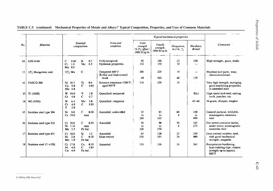
Properties of Solid
sC
-43
© 1999 by CRC Press LLC
TABLE C.5 (continued) Mechanical Properties of Metals and Alloys:* Typical Composition, Properties, and Uses of Common Materials

C-44
Appen
dix C
© 1999 by CRC Press LLC
TABLE C.5 (continued) Mechanical Properties of Metals and Alloys:* Typical Composition, Properties, and Uses of Common Materials

Properties of Solid
sC
-45
© 1999 by CRC Press LLC
TABLE C.5 (continued) Mechanical Properties of Metals and Alloys:* Typical Composition, Properties, and Uses of Common Materials

C-46
Appen
dix C
© 1999 by CRC Press LLC
TABLE C.5 (continued) Mechanical Properties of Metals and Alloys:* Typical Composition, Properties, and Uses of Common Materials

Properties of Solid
sC
-47
© 1999 by CRC Press LLC
TABLE C.5 (continued) Mechanical Properties of Metals and Alloys:* Typical Composition, Properties, and Uses of Common Materials
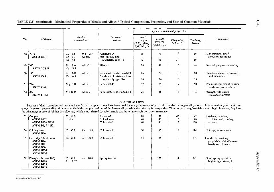
C-48
Appen
dix C
© 1999 by CRC Press LLC
TABLE C.5 (continued) Mechanical Properties of Metals and Alloys:* Typical Composition, Properties, and Uses of Common Materials

Properties of Solid
sC
-49
© 1999 by CRC Press LLC
TABLE C.5 (continued) Mechanical Properties of Metals and Alloys:* Typical Composition, Properties, and Uses of Common Materials
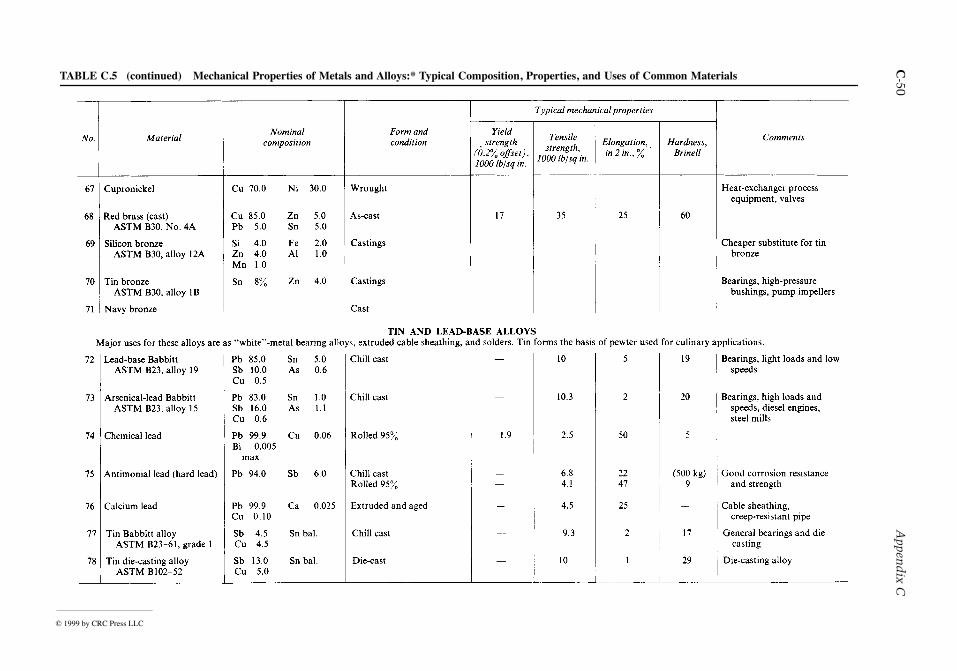
C-50
Appen
dix C
© 1999 by CRC Press LLC
TABLE C.5 (continued) Mechanical Properties of Metals and Alloys:* Typical Composition, Properties, and Uses of Common Materials
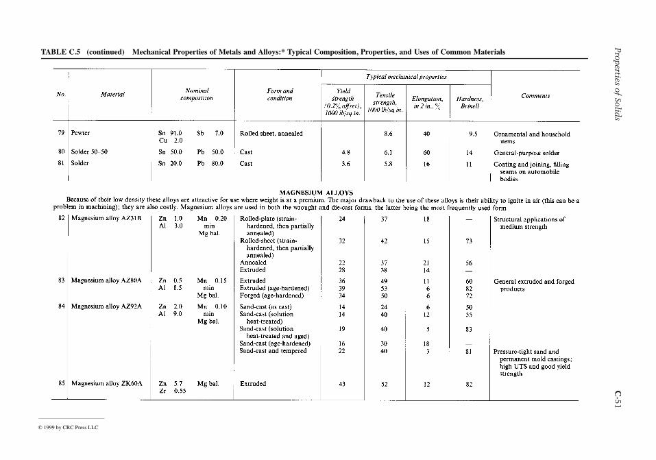
Properties of Solid
sC
-51
© 1999 by CRC Press LLC
TABLE C.5 (continued) Mechanical Properties of Metals and Alloys:* Typical Composition, Properties, and Uses of Common Materials
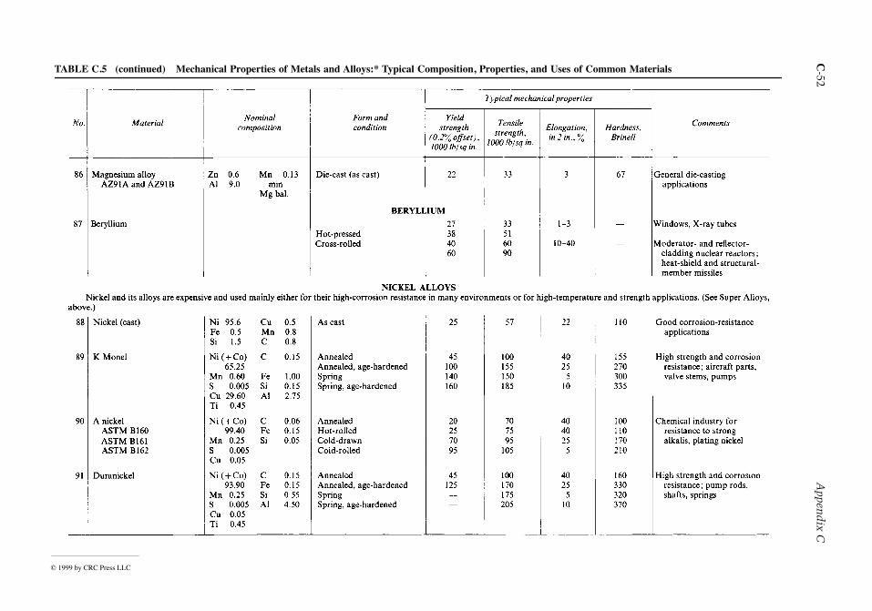
C-52
Appen
dix C
© 1999 by CRC Press LLC
TABLE C.5 (continued) Mechanical Properties of Metals and Alloys:* Typical Composition, Properties, and Uses of Common Materials

Properties of Solid
sC
-53
© 1999 by CRC Press LLC
TABLE C.5 (continued) Mechanical Properties of Metals and Alloys:* Typical Composition, Properties, and Uses of Common Materials

C-54
Appen
dix C
© 1999 by CRC Press LLC
TABLE C.5 (continued) Mechanical Properties of Metals and Alloys:* Typical Composition, Properties, and Uses of Common Materials

Properties of Solids C-55
© 1999 by CRC Press LLC
TABLE C.6 Miscellaneous Properties of Metals and Alloys
Part a. Pure MetalsAt Room Temperature

C-56 Appendix C
© 1999 by CRC Press LLC
TABLE C.6 Miscellaneous Properties of Metals and Alloys
Part b. Commercial Metals and Alloys

Properties of Solids C-57
© 1999 by CRC Press LLC
TABLE C.7 Composition and Melting Points of Binary Eutectic Alloys:* Binary Alloys and Solid Solutions of Metallic Components

C-58 Appendix C
© 1999 by CRC Press LLC
TABLE C.7 (continued) Composition and Melting Points of Binary Eutectic Alloys:* Binary Alloys and Solid Solutions of Metallic Components

Properties of Solids C-59
© 1999 by CRC Press LLC
TABLE C.8 Melting Points of Mixtures of Metals**
TABLE C.7 (continued) Composition and Melting Points of Binary Eutectic Alloys:* Binary Alloys and Solid Solutions of Metallic Components

C-60 Appendix C
© 1999 by CRC Press LLC
TABLE C.9 Trade Names, Composition, and Manufacturers of Various Plastics

Properties of Solids C-61
© 1999 by CRC Press LLC
TABLE C.9 (continued) Trade Names, Composition, and Manufacturers of Various Plastics

C-62 Appendix C
© 1999 by CRC Press LLC
TABLE C.10 Properties of Commercial Nylon Resins*
For Conversion factors see Table C.10.

Properties of Solids C-63
© 1999 by CRC Press LLC
TABLE C.11 Properties of Silicate Glasses*

C-64 Appendix C
© 1999 by CRC Press LLC
Corning Glass Works code numbers are used in this table.
TABLE C.11 (continued) Properties of Silicate Glasses*

Properties of Solids C-65
© 1999 by CRC Press LLC
TABLE C.11 (continued) Properties of Silicate Glasses*

C-66 Appendix C
© 1999 by CRC Press LLC
TABLE C.12 Properties of Window Glass*: Transmittance of Sheet and Plate Glass

Properties of Solids C-67
© 1999 by CRC Press LLC
TABLE C.13 Properties and Uses of American Woods*

C-68 Appendix C
© 1999 by CRC Press LLC
TABLE C.13 (continued) Properties and Uses of American Woods*

Properties of Solids C-69
© 1999 by CRC Press LLC
Note: For weight-density in kg/m3, multiply value in lb/ft3 by 16.02.
TABLE C.13 (continued) Properties and Uses of American Woods*

C-70 Appendix C
© 1999 by CRC Press LLC
TABLE C.14 Properties of Natural Fibers*
Because there are great variations within a given Þber class, average properties may be misleading. The followingtypical values are only a rough comparative guide.

Properties of Solids C-71
© 1999 by CRC Press LLC
TABLE C.15 Properties of Manufactured Fibers*

C-72 Appendix C
© 1999 by CRC Press LLC
TABLE C.16 Properties of Rubbers and Elastomers*

Properties of Solids C-73
© 1999 by CRC Press LLC
TABLE C.16 (continued) Properties of Rubbers and Elastomers*

D-74 Appendix D
© 1999 by CRC Press LLC
Appendix D. Gases and Vapors
TABLE D.1 SI Units Ñ DeÞnitions, Abbreviations and PreÞxes
DAppendix D
Gases and Vapors

Miscellaneous E-75
© 1999 by CRC Press LLC
Appendix E. Miscellaneous
TABLE E.1 Sizes and Allowable Unit Stresses for Softwood Lumber
American Softwood Lumber Standard. A voluntary standard for softwood lumber has been developing since 1922.Five editions of SimpliÞed Practice Recommendation R16 were issued from 1924Ð53 by the Department of Commerce;the present NBS voluntary Product Standard PS 20-70, ÒAmerican Softwood Lumber StandardÓ, was issued in 1970. Itwas supported by the American Lumber Standards Committee, which functions through a widely representative NationalGrading Rule Committee.
Part a. Nominal and Minimum-Dressed Sizes of Lumber*
Note: This table applies to boards, dimensional lumber, and timbers. The thicknesses apply to all widths and all widths to all thicknesses.
EAppendix E
Miscellaneous

E-76 Appendix E
© 1999 by CRC Press LLC
TABLE E.1 (continued) Sizes and Allowable Unit Stresses for Softwood Lumber
The ÒAmerican Softwood Lumber StandardÓ, PS 20-70, gives the size and grade provisions for American Standard lumberand describes the organization and procedures for compliance enforcement and review. It lists commercial nameclassiÞcations and complete deÞnitions of terms and abbreviations.Eleven softwood species are listed in PS 20-70, viz., cedar, cypress, Þr, hemlock, juniper, larch, pine, redwood, spruce,
tamarack, and yew. Five dimensional tables show the standard dressed (surface planed) sizes for almost all types of lumber,including matched tongue-and-grooved and shiplapped ßooring, decking, siding, etc. Dry or seasoned lumber must have19% or less moisture content, with an allowance for shrinkage of 0.7Ð1.0% for each four points of moisture content belowthe maximum. Green lumber has more than 19% moisture. Table A illustrates the relation between nominal size and dressedor green sizes.National Design SpeciÞcation. Part b is condensed from the 1971 edition of ÒNational Design SpeciÞcation for Stress-Grade Lumber and Its Fastenings,Ó as recommended and published by the National Forest Products Association, Washington,D.C. This speciÞcation was Þrst issued by the National Lumber Manufacturers Association in 1944; subsequent editionshave been issued as recommended by the Technical Advisory Committee. The 1971 edition is a 65-page bulletin with a20-page supplement giving ÒAllowable Unit Stresses, Structural Lumber,Ó from which Part b has been condensed. The dataon working stresses in this Supplement have been determined in accordance with the corresponding ASTM Standards,D245-70 and D2555-70.
Part b. Species, Sizes, Allowable Stresses, and Modulus of Elasticity of Lumber
Normal loading conditions: Moisture content not over 19%, No. 1 grade, visual grading. To convert psi to N/m2, multiply
by 6 895.
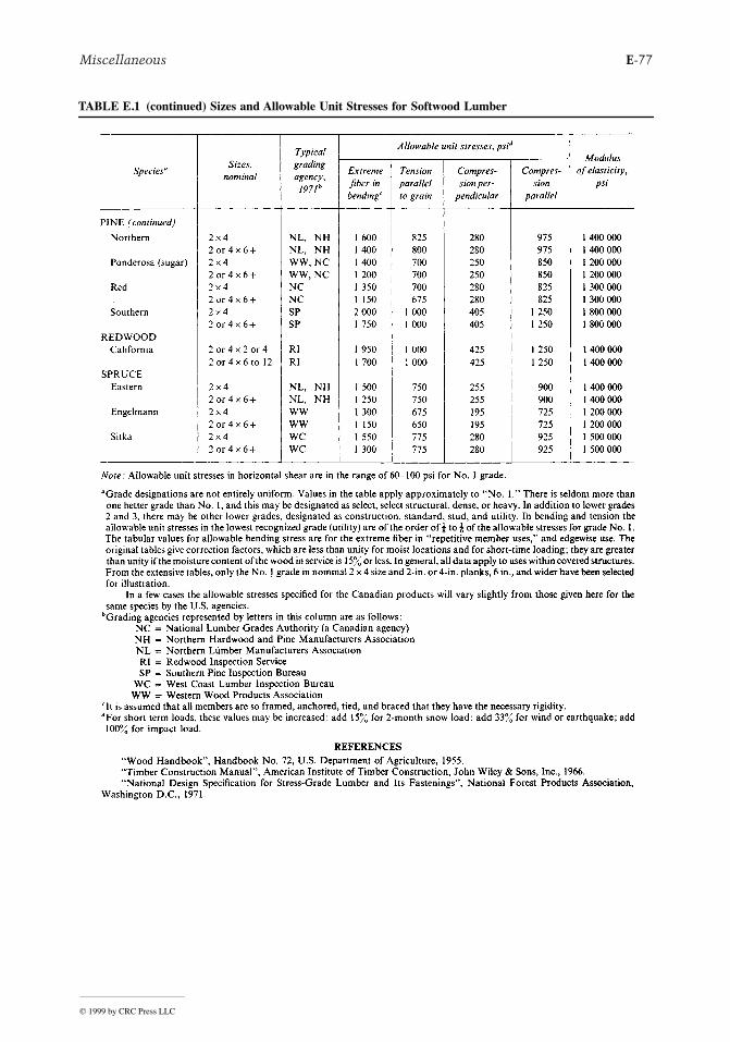
Miscellaneous E-77
© 1999 by CRC Press LLC
TABLE E.1 (continued) Sizes and Allowable Unit Stresses for Softwood Lumber

E-78 Appendix E
© 1999 by CRC Press LLC
TABLE E.2 Standard Grades of Bolts
Part a: SAE Grades for Steel Bolts

Miscellaneous E-79
© 1999 by CRC Press LLC
TABLE E.2 (continued) Standard Grades of Bolts
Part b: ASTM Grades for Steel Bolts

E-80 Appendix E
© 1999 by CRC Press LLC
Part c: Metric Mechanical Property Classes for Steel Bolts, Screws, and Studs
TABLE E.2 (continued) Standard Grades of Bolts
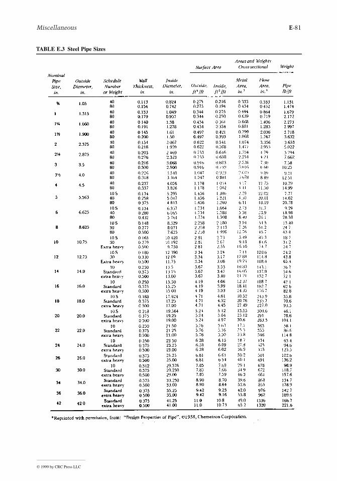
Miscellaneous E-81
© 1999 by CRC Press LLC
TABLE E.3 Steel Pipe Sizes
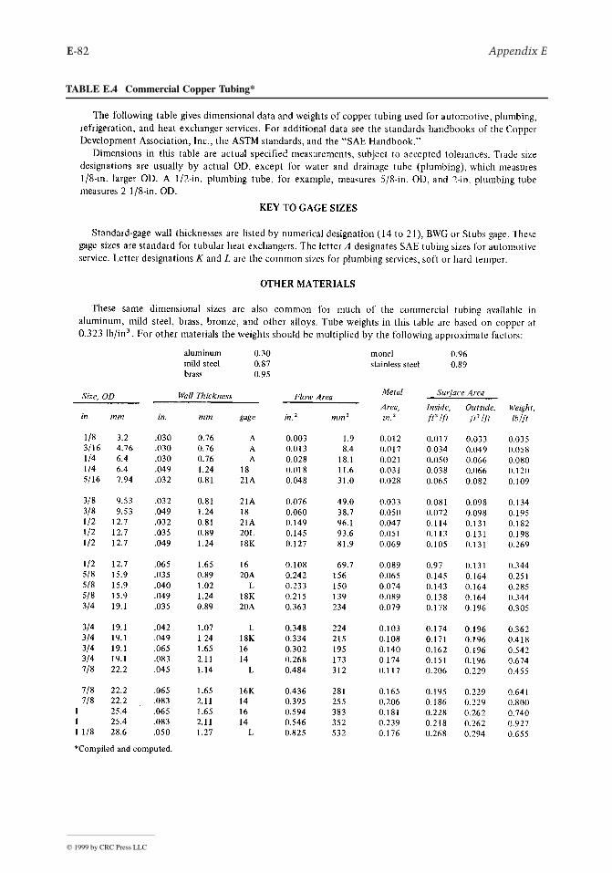
E-82 Appendix E
© 1999 by CRC Press LLC
TABLE E.4 Commercial Copper Tubing*

Miscellaneous E-83
© 1999 by CRC Press LLC
TABLE E.4 (continued) Commercial Copper Tubing*

E-84 Appendix E
© 1999 by CRC Press LLC
TABLE E.5 Standard Gages for Wire, Sheet, and Twist Drills
Dimensions in approximate decimals of an inch.
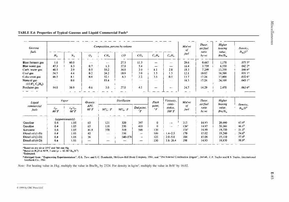
Miscellan
eous
E-85
© 1999 by CRC Press LLC
TABLE E.6 Properties of Typical Gaseous and Liquid Commercial Fuels*
Note: For heating value in J/kg, multiply the value in Btu/lbm by 2324. For density in kg/m3, multiply the value in lb/ft3 by 16.02.

E-86 Appendix E
© 1999 by CRC Press LLC
TABLE E.7 Combustion Data for Hydrocarbons*
Note: For heating value in J/kg, multiply the value in Btu/lbm by 2324. For ßame speed in m/s, multiply the value in ft/s by 0.3048.
Copyright © 2022 FDOKUMEN