Iterative Formalization of Smallest Workface Boundary for Generating

Daily Bills of Materials

By

Min Song & Martin Fischer

CIFE Working Paper #WP144 January 2019

STANFORD UNIVERSITY

COPYRIGHT © 2019 BY Center for Integrated Facility Engineering

If you would like to contact the authors, please write to:

c/o CIFE, Civil and Environmental Engineering Dept., Stanford University

The Jerry Yang & Akiko Yamazaki Environment & Energy Building 473 Via Ortega, Room 292, Mail Code: 4020

Stanford, CA 94305-4020

Iterative formalization of smallest workface boundary for generating daily bills of materials

Abstract A study on 831 daily work orders collected from five construction sites showed that a foreman can generate a bill of materials (BOM) quickly for daily work orders consisting of engineered-to-order (ETO) materials but that for daily work orders consisting of made-to-stock (MTS) materials, the process can be time consuming (e.g., 12-68 minutes per daily BOM). To help a foreman expedite the speed of generating a daily BOM consisting of MTS materials, this research develops a concept referred to as a smallest workface boundary (SWFB)—a boundary that encapsulates a set of level of development (LOD) 400 elements in the smallest workable unit for a certain trade with the objective of assisting a foreman in quickly generating a daily BOM. Through iterative field studies at a lab and nine construction sites, the concept of SWFB was developed, tested with foremen, and incrementally improved to speed up the process of generating a daily BOM for a foreman. With the latest version of the prototype, foremen were able to generate a daily BOM in 59 seconds on average. Author keywords: Bill of materials; Daily work order; Building information modeling; Level of development; Smallest workface boundary

Introduction A comprehensive daily work order issued to a construction crew has location information, reference drawings, a bill of materials, lists of equipment and workforce needed, a method description, and date information (Oglesby et al. 1989; Mourgues 2008). The construction industry is increasingly interested in implementing a daily work order (McGraw-Hill Construction 2013), but for a foreman, whose priority is managing fabrication work in progress at the field, generating a work order containing all of this information on a daily basis can be challenging. This is especially true for the information item “bill of materials” among others. A bill of materials (BOM) is a list of materials required to build a product (Clement et al. 1992; Popov et al. 1997; Zhao 2015). In order for a foreman to prepare a complete list of materials, the foreman has to refer to a fabrication level of drawing, i.e., a shop drawing, since this is the document that describes a fully engineered product with all components necessary for fabrication. But for the foreman, this process of referring to a shop drawing and generating a daily BOM can be time consuming. The time to generate a BOM can vary depending on the construction work at hand, but the field observations done in a previous study (Song et al. 2017) shows that it depends on the types of materials. The time to generate a daily BOM is typically longer when the materials involved in the BOM are MTS materials—the types of materials that are stocked at a site and further processed at the site through cutting, bending, fabricating, or applying. To help a foreman in quickly generating a daily BOM consisting of MTS materials, this paper formalizes the concept of a smallest workface boundary (SWFB): a boundary that encapsulates a set of level of development (LOD) 400 elements (AIA 2013) in the smallest workable unit for a certain trade. This paper describes how the concept of SWFB was iteratively improved through prototyping and executing field experiments where foremen were given the prototype for generating a daily BOM. Generating a BOM is time-consuming, and a foreman often does not have the time to do so on a daily basis. However, if this process can be made faster, it can become a basis for enabling precise control over the field. It can allow a foreman to plan where the materials should be, in what amount, and by which date—thereby establishing a precise baseline. It can also allow site people to delay the delivery of

materials until the last moment of installation, reducing unnecessary stacking and movement of materials. Furthermore, it can help generating refined controls metrics that are derived based on the quantities, such as production rate (when the BOM information is tied to manpower information) and percent plan complete (PPC) that can be drilled down to and analyzed on a daily level. To achieve this, a foreman first should be able to quickly generate a daily BOM. This paper describes a concept for enabling this—a SWFB.

Observed problem and points of departure

Types of materials At the start of this research in 2016, the authors conducted field observation at five construction sites where daily work orders were being produced by foremen. A total of 831 daily work orders were collected from the five sites and analysis on them showed that a daily BOM is not included in a daily work order. Then further analysis was done to see whether a foreman can quickly generate a daily BOM using the information resources available at the sites. The finding was that the availability of information depends on the types of materials associated with a BOM. In particular, the materials could be grouped into two types: engineered-to-order (ETO) types of materials and made-to-stock (MTS) types of materials. ETO materials are the types of materials that are engineered and fabricated upfront in a supply chain; MTS materials are the types of materials that are stocked at a site and further processed at the site through cutting, bending, fabricating, or applying. Examples of ETO materials are unitized curtain walls, structural steel, and pipe spools; examples of MTS materials are track and studs, sheetrock, concrete blocks, wood, and paint. (Further distinction between ETO and MTS can be found in (Sharman 1984).) The analysis on the generation of a daily BOM showed that when the BOM consists of ETO materials, generating a daily BOM can be done within a few minutes because ETO materials tend to be engineered and fabricated upfront before reaching the site, and this drives the suppliers to generate a product-specific shop drawing, which often has a BOM available at one corner of the shop drawing. By accessing this ready-made information prevalent in ETO materials, a foreman can generate a daily BOM quickly. In contrast, for MTS materials, a typical shop drawing (rather than a product-specific shop-drawing) is usually provided, and a foreman has to go through the additional process of manual takeoff based on the typical shop drawing. Sample tests with foremen at construction sites showed that the time to generate a daily BOM consisting of MTS materials is in the range of 12 - 68 minutes per daily BOM.

Level of development The second analysis on 831 daily work orders collected from the five sites was about the feasibility of BIM-based takeoff for generating a daily work order. This involved going through 831 daily work orders collected from the five sites and checking whether corresponding 3D elements of each daily work order exist in the BIM or not. The analysis showed a contrast between level of development (LOD) 300 and LOD 400. It showed that when LOD 300 is used, only 29% of the daily work orders have corresponding elements in BIM, but when LOD 400 is used, 98% of the daily work orders have corresponding elements in BIM. The finding related to this contrast between LOD 300 and LOD 400 is further described in Song et al. (2017).

Prior studies In the literature, there have been studies on controlling the flow of materials which requires a BOM. Song et al. (2017) point out that these studies include the pipe spool case in Tommelein (1998), the precast concrete case in Ergen et al. (2007), the pipe spool case in Song et al. (2006), and the prefabricated structural component case in Wang et al. (2007). One notable fact is that these studies relate to the types of materials that involve a certain degree of upfront engineering and fabrication, which makes them relevant to ETO materials. In contrast, to the best of the authors’ knowledge, there are no formal studies on generating a daily BOM consisting of MTS materials.

Regarding daily work orders, Oglesby et al. (1989) provide a generic insight into the formation of a daily work order, referred to as a job-assignment sheet in the literature, but the book lacks formal study (as Mourgues (2008) points out). The Last Planner application developed by the construction company DPR (now BIM 360 Plan, acquired by Autodesk) is on the level of describing the daily units of work, but the application does not establish a relationship between the description and a BIM. Sacks et al. (2010), on the other hand, uses a BIM and relates BIM elements with daily work descriptions, but the study is not focused on the use of LOD 400. Mourgues (2008) formalizes a model for generating a daily work order. This model builds on the OAR (Object-Action-Resource) model and the CARS (Component-Action-Resource-Sequencing) model, previously developed by Darwiche et al. (1989) and Aalami (1998), respectively. However, Mourgues (2008) focuses on rebar, which is ETO and for which there is typically a bar bending schedule available allowing for the quick generation of a BOM. The analyses on 831 daily work orders and literature review suggest that if one is to research a system for quickly generating a daily BOM, the research should focus on addressing the problem related to MTS materials and consider using LOD 400 elements. In line with this, the research in this paper attempts to answer the question of “how can a foreman quickly generate a daily BOM consisting of MTS materials using LOD 400 elements?”

Research method A daily work order or BOM at a construction site should be prepared by a person who thoroughly knows and manages a day's work of a trade. Hence interaction with a foreman was required in this research. This research comprised two types of field studies. One was field observation, where there was no intervention at the site and only observations and interviews were carried out. The other was field experiments, where a field intervention was made for testing a prototype and receiving feedback. Between the field experiments, prototyping was done at a research lab in an iterative process using the findings to improve the prototype and retesting successive versions of the prototype in the next field experiment, with the goal of reducing the time it takes for a foreman to generate a daily BOM. Fig. 1 shows the iterative field studies. The first five field observations in the figure were dedicated to finding a problem and points of departure. The findings of these five field observations are briefly summarized in the previous section and the details are documented in Song et al. (2017). Based on the problem identification and points of departure study, prototyping started intuitively with the use of LOD 400 elements for generating a daily BOM. When a certain version of a prototype was ready, a field experiment took place for a period of three weeks where the prototype was given to a foreman for generating a daily BOM consisting of MTS materials. For operating the prototype, an interactive board was installed at a site office or in a building under construction. The first of the three weeks was generally spent on getting the experiment ready by selecting trades involving MTS materials and importing LOD 400 elements to the prototype. In the remaining two weeks, foremen used the prototype for generating daily BOMs and the time to generate each daily BOM was recorded. The research repeated this cycle (i.e., reflecting on previous field findings, improving the prototype, and applying a new version of the protype to the next field experiment).

Fig. 1. Iterative field studies: with the problem identification and points of departure study from the first 5 field observations, the concept of a SWFB was iteratively developed and improved over the course of field observation 06 and field experiment 01 thru 03

First prototype using LOD 400 elements

Given the findings from analyzing 831 daily work orders collected from field observation 01 thru 05, the next logical step was to build a prototype that imports LOD 400 elements. This prototype was envisioned to be installed in a site office where a foreman can work with an interactive board with touch capabilities. The board had multiple viewports, and each viewport was dedicated to a single trade and displayed LOD 400 elements relevant to that trade. Fig. 2 shows the first version of the prototype, which was tested in a lab setting. This stage corresponds to the “Prototype v1” stage in Fig. 1.

Fig. 2. First version of the prototype: in each viewport, trade-specific LOD 400 elements were shown, and a user could select a set of LOD 400 elements and convert them into a daily BOM (card)

The problem with this prototype was that there were too many 3D elements to select from. The basic workflow for a user was to select a set of 3D elements from the viewport and convert these elements into a daily BOM (represented as a card on the display shown in Fig. 2). However, since the elements in the viewport are at LOD 400, there were too many elements to select from. For instance, a single interior wall modeled at LOD 400 may have around 180 elements including all the screws and frames. Selecting these elements individually by tapping on them did not make sense. To overcome this repetitive input, another approach that was tested was letting a user draw a free boundary that could be adjusted and selecting all the elements within the boundary. But this approach also turned out to be inconvenient, because a user

had to consistently check whether the edges of the boundaries were adjusted and placed correctly to include or exclude the small connection elements, such as screws or brackets, and this required a user to think, adjust, and maneuver around the 3D view multiple times. From this point, the prototyping evolved to questioning how to group the granular LOD400 elements into a unit of work for a faster generation of a daily BOM. The theories developed by researchers (Hopp and Spearman 1996; O’Brien 1998; Morkos 2014; Ballard and Tommelein 1999; Walsh et al. 2004; Sacks and Goldin 2007; Ballard and Choo 2011) shed light on how this question may be answered. Their theories have shown that creating a smaller batch size improves the performance of a production system in terms of reducing cycle time and risk. Reflecting on their theories, the authors of this paper arrived at the idea of grouping LOD400 elements into a smaller unit of work. One concern in doing so was that, in construction, there is a limitation on how much the size of a unit of work can be reduced. For instance, it does not make sense to work in the unit of one linear foot for installing track and studs of a drywall. To study this limitation, an observation was done at a site to determine whether identifying a smallest unit of work for a certain trade is feasible or not.

Field observation 06 and formation of SWFB Field observation 06 took place at a residential construction site in the US. The construction was at an interior stage for the first building and at a concrete structure stage for the second building. The purpose of this field observation was to follow the construction crews of different trades and identify the smallest unit of work per task. Forty-six tasks were observed at the site, and, based on the observation and interviews with the crews, it was feasible to identify the smallest unit of work for forty-two tasks (for the remaining four tasks, a larger unit of work was preferable due to concrete curing time since splitting pour areas and having multiple curing days did not reduce the work duration). The smallest unit of work tended to be different between tasks. For track and studs, the smallest unit of work was a wall; for painting, the smallest unit of work was a room; for piping, the smallest unit of work was a pipe component plus the connection parts (e.g., elbows/tees) at two ends of the pipe, and so on. Following field observation 06, the concept of a smallest workface boundary (SWFB) was developed in a lab environment. This corresponds to the “Prototype v2” stage in Fig. 1. In this research, a SWFB is defined as the boundary that encapsulates a set of LOD 400 elements in the smallest workable unit for a certain trade. (Note that the terminology “workface” has nothing to do with the “workface” in “workface planning” of the CII Research Team 272-1 (2011).) In what follows, an algorithm for generating a SWFB is explained with a piping case. A piping case is used as an example here because the algorithm for generating a SWFB for piping elements has a greater number of steps and greater complexity than the algorithms of other trades’ elements. Developing an algorithm for automatically generating a SWFB starts with a discussion with a foreman. For instance, in case of the piping work observed in field observation 06, the smallest unit of work was identified as a pipe component plus the connection parts (e.g., elbows/tees) at two ends of the pipe. In this case, a SWFB is defined by a boundary in a 3D space that encapsulates the pipe element and the connecting elements at two ends of the pipe. The steps for generating this boundary are illustrated in Fig. 3. The top-left image of Fig. 3 shows the scope of the example. There are in total 10 elements in the scope: 4 coupling elements, 2 elbow elements, 2 elbow insulation elements, 1 pipe element, and 1 pipe insulation element.

Fig. 3. Steps for generating a SWFB for a piping trade: a SWFB is generated by first finding a dominant vector direction, making a primitive cube and rotating it to align with the dominant vector direction, and extending the cube to include the connection parts (e.g., elbows)

Step 1. Find dominant vector direction: For piping elements, the “pipe” element is the reference element for generating a SWFB. In step 1 of Fig. 3, this pipe element is rendered in wireframe (i.e., illustrated with edge lines that form the geometry). These edge lines are collapsed into vectors. In the figure, these vectors point outward from the origin of the world axis. Then the number of vectors pointing in the same direction are counted. In the figure, “16” is the highest number, and therefore the vector pointing to “16” indicates the dominant vector direction, which is the direction that aligns with the direction of the pipe element. (Note that another way of finding this direction is by computing an eigen vector, but computing an eigen vector is computationally more expensive, especially when there is a large number of pipe elements in the 3D model.) Step 2. Align a local axis to the dominant vector direction: In this step, the world axis (expressed by XYZ in the figure) is rotated to align with the dominant vector direction. This rotated axis becomes the local axis aligned with the pipe direction (i.e., the dominant vector direction). Then the unit vectors (expressed by UVW in the figure) of the local axis are used to create a transformation matrix (1). The role of the transformation matrix is to rotate a vertex by the same amount of the rotation executed when going from the world axis to the local axis—this transformation matrix is used in the next step.

�

0.962 0 −0.272 00 1 0 0

0.272 0 0.962 00 0 0 1

� �

𝑥𝑥𝑦𝑦𝑧𝑧1� (1)

Step 3. Create a primitive cube and rotate it to align with the dominant vector direction: This step creates a primitive cube, which later will be turned into a SWFB. The primitive cube is rotated to align with the dominant vector direction. This also means that the primitive cube is aligned with the pipe direction. To rotate the cube, the transformation matrix is multiplied by each of the 8 vertices of the cube. The equation below shows the matrix multiplication for one vertex (0.05, 0.05, -0.05) as an example.

�

0.962 0 −0.272 00 1 0 0

0.272 0 0.962 00 0 0 1

� �

0.050.05−0.05

1� = �

0.06170.05

−0.03451

� (2)

Step 4. Move the rotated primitive cube to the center of the pipe element: After the rotation for 8 vertices is done at the origin of the world axis, the rotated primitive cube is moved to the center of the pipe element as shown in step 4 of Fig. 3.

�

1 0 0 −6.80 1 0 1.40 0 1 −1.20 0 0 1

� �

0.06170.05

−0.03451

� = �

−6.73831.45

−1.23451

� (3)

Step 5. Extend the cube to encapsulate the pipe and connection elements (i.e., the elbow elements): First, the primitive cube at the center of the pipe is extended to encapsulate the pipe element. Then the extension is further made to encapsulate the connection parts (elbow elements) at two ends of the pipe element. In this construction project, all the elbows were less than 0.3m in length, so the second extension is done by 0.3m. The bottom-right image of Fig. 3 shows the final SWFB generated encapsulating 10 elements. In a field setting when a foreman is using SWFBs, the benefit is that the foreman can select a SWFB (a predefined boundary) instead of selecting individual elements. This speeds up the process of scoping a day’s work (i.e., selecting a certain scope of elements) thereby helping a foreman to quickly generate a daily BOM. The algorithm for generating SWFBs was programmed in prototype v2 and this version was tested in a field setting. In what follows, three field experiments are described. In each field experiment, a prototype was provided to a foreman in charge of a certain trade and the task was to generate daily BOMs as described in the Research Method section of this paper. In the field setting, an interactive board was installed, and foremen used the interactive board to select SWFBs (which contain LOD 400 elements) to define a day’s scope of work. Then in the prototype, a daily BOM was automatically generated based on the selected SWFBs which contains LOD 400 elements.

Field experiment 01 using SWFB Field experiment 01 was on an airport, and the trades tested were ceiling, glass, and mechanical piping. The materials of the ceiling frames and mechanical piping were both MTS types, which were cut and fixed at the site. The materials of the glass trade were a mix of ETO and MTS materials. The glass panels were ETO materials with a unique material code, but the connection parts (angle brackets) were MTS materials. This stage of the research corresponds to the “Field experiment 01” stage in Fig. 1.

In this experiment, the first finding while focusing on the ceiling trade was that engineering decisions of a trade can affect the shape of a SWFB. In case of the ceiling trade, the C-channels (i.e., the rails of the ceiling frame) were engineered in the units of 3000mm, meaning that each C-channel installed was in the length of 3000mm (see the ceiling trade in Fig. 4). Once the C-channels (rails) were installed, the bridging studs @300mm were installed between the rails as shown in the figure. The foreman said that two to three units (one unit being 3000mm in length including the bridging studs) can be installed in a day and suggested that the SWFB should follow the dimension of the C-channels and should be formed to encapsulate each unit of C-channel, as shown in the ceiling trade in Fig. 4. Hence in this case, the C-channels served as a reference element for shaping a SWFB. For the glass trade in this experiment, determining the reference element was straightforward. The installation was done in the units of glass panels, and each glass panel served as a reference element for shaping a SWFB (see the glass trade in Fig. 4). And from the outer lines of the reference element, an offset of 300mm was made to shape a SWFB—the offset was to include the connection parts (angle brackets) that hold the glass panels. For the mechanical piping trade, a pipe (the straight portion in piping) served as a reference element for shaping a SWFB. The steps for generating a SWFB described in the previous section are based on this trade. As described previously, a SWFB in this case is a boundary encapsulating a pipe element and the connecting elements (e.g., elbows/tees) at two ends of the pipe.

Fig. 4. SWFBs generated in field experiment 01: the boxes drawn with bold edge lines are SWFBs; the shape of the SWFB for the ceiling trade was driven by the length of a C-channel element; the shape of the SWFB for the glass trade by a glass panel element; and the shape of the SWFB for the mechanical piping trade by a pipe element

Limitations observed in field experiment 01

A notable finding from field experiment 01 was that 7 daily BOMs (cards) out of a total of 46 took substantially longer to generate than the remaining cards (called out in Fig. 8). The difference between these 7 cards and the rest of the cards was that, for the 7 cards, the foreman had to segregate a set of elements that were to be installed on a different day from the rest of the elements within the same SWFB. In other words, the process of generating a card took longer when the elements in a SWFB were to be installed in multiple phases. To illustrate, Fig. 5 shows a case where this phasing problem was present. In

this SWFB, the pipes, elbows, and couplings were to be installed on day 1 (phase 1), and the insulation covering these elements were to be installed on day 7 (phase 2). The phasing was necessary because a hydro test needs to be done between the two phases. The 7 cards took longer to generate because when a foreman used a SWFB, the SWFB fetched all the elements within the SWFB, and after all the elements were selected, the foreman then again had to deselect the elements individually to exclude the elements that fell into a different phase. Based on the observed shortcoming, the next version (v3) of the prototype was made to allow a foreman to either select all elements within a SWFB or select a certain type of elements (e.g., all insulation elements) within a SWFB to help the phasing of the elements. This stage corresponds to the “Prototype v3” stage in Fig. 1.

Fig. 5. A case where a SWFB contains elements installed in two different phases

Field experiment 02 & 03 using SWFB and phasing functionality

Field experiment 02

Field experiment 02 was on a residential project, and the trades tested were facade, planter wooden frame, and protective concrete. The materials of facade and protective concrete were both MTS types—stacked and fabricated/installed on site. The materials of the planter trade were a mix of ETO and MTS materials. The planter boxes (steel frames) were ETO materials with unique material code, but the wooden frames fabricated on the exterior of the planter boxes were MTS materials. LOD400 elements were originally not available for the project, but for the field experiment, a roof construction area was selected and details were developed into LOD400. Fig. 6 shows the construction area. In this experiment, the facade trade had a phasing issue (similar to the one observed in the mechanical piping trade in field experiment 01). A SWFB for the facade trade was generated based on a wall object, as shown in the facade trade of Fig. 6, and in this SWFB there were screw type A, membrane, profiles, screw type B, and cedar wood elements. Among these elements screw type A, membrane, and profiles were substrates so these were installed first, and after around 10 days, the remaining elements, screw type B and cedar wood elements, were installed on top of the substrates. With prototype v3, a foreman was able to differentiate the selection by phases and select only a certain type of elements within a SWFB. After the experiment, the average time to generate a daily BOM card for the facade trade was 37 seconds, which was much lower than the average of 7 minutes and 24 seconds observed in the mechanical piping trade (the trade that had a similar phasing issue) in the previous experiment. In prototype v3, we also built a functionality of adding the number of workers to each daily BOM. When highlighting LOD 400 elements to be built on a certain day on the prototype display, the workers were also visualized next to the LOD 400 elements. This turned out to be helpful for cross checking the areas occupied by the workers on a certain day and preventing clashes between different trades’ workers in the same area.

Fig. 6. SWFBs generated in field experiment 02: the shape of the SWFB for the facade trade was driven by a wall element; the shape of the SWFB for the planter trade by a planter box element; and the shape of the SWFB for the protective concrete trade by a concrete element

Field experiment 03

Field experiment 03 was on a residential project, and the trades tested were masonry, electrical conduit, and water piping. All the materials of the trades were MTS types. On this project, the elements of the electrical conduit and water piping trades were modeled at LOD400. However, the elements of the masonry trade were modeled at LOD300. Therefore, during the 3 weeks of visit to the site, the first 2 weeks were focused on modeling LOD400 elements for masonry, testing interoperability, and setting up the prototype. At the time of the visit, the construction work of the trades was in progress on floor 2 through floor 5. On this project, there was a discussion on how to shape the SWFB for electrical conduits and water piping. For these two trades, one option was to use the method we used in field experiment 01 for mechanical piping, where a SWFB was determined by a pipe element and extended to include connection parts at two ends of the pipe, such as an elbow or a tee. Another option was to use a wall object as a SWFB for electrical conduits and water piping. After discussion, it made more sense to use the wall object as a reference element for generating a SWFB, as shown in Fig. 7, because the electrical and plumbing rough-ins were built in the units of walls to make a unit of a wall ready for the succeeding masonry trade to work. In field experiment 01, the mechanical pipes were not installed inside a wall, and the elements were spread across the ceiling, so shaping a SWFB to encapsulate a pipe and connection parts (elbows/tees) made more sense.

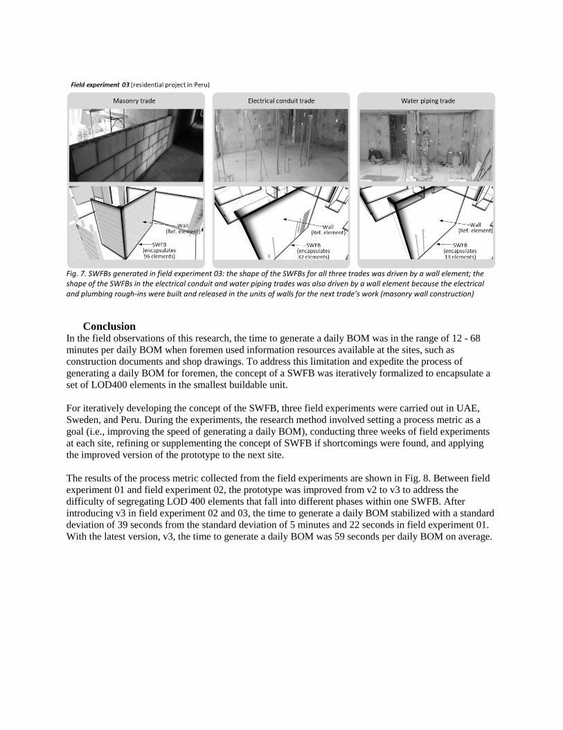
Fig. 7. SWFBs generated in field experiment 03: the shape of the SWFBs for all three trades was driven by a wall element; the shape of the SWFBs in the electrical conduit and water piping trades was also driven by a wall element because the electrical and plumbing rough-ins were built and released in the units of walls for the next trade’s work (masonry wall construction)

Conclusion

In the field observations of this research, the time to generate a daily BOM was in the range of 12 - 68 minutes per daily BOM when foremen used information resources available at the sites, such as construction documents and shop drawings. To address this limitation and expedite the process of generating a daily BOM for foremen, the concept of a SWFB was iteratively formalized to encapsulate a set of LOD400 elements in the smallest buildable unit. For iteratively developing the concept of the SWFB, three field experiments were carried out in UAE, Sweden, and Peru. During the experiments, the research method involved setting a process metric as a goal (i.e., improving the speed of generating a daily BOM), conducting three weeks of field experiments at each site, refining or supplementing the concept of SWFB if shortcomings were found, and applying the improved version of the prototype to the next site. The results of the process metric collected from the field experiments are shown in Fig. 8. Between field experiment 01 and field experiment 02, the prototype was improved from v2 to v3 to address the difficulty of segregating LOD 400 elements that fall into different phases within one SWFB. After introducing v3 in field experiment 02 and 03, the time to generate a daily BOM stabilized with a standard deviation of 39 seconds from the standard deviation of 5 minutes and 22 seconds in field experiment 01. With the latest version, v3, the time to generate a daily BOM was 59 seconds per daily BOM on average.

Fig. 8. The time a foreman spent on generating a daily BOM card using the prototype: in field experiment 01, prototype v2 was used and in field experiment 02 and 03, prototype v3 was used; the average time it took a foreman to generating a daily BOM with the latest version, v3, was 59 seconds per daily BOM; a video clip of foremen generating daily BOMs with prototype v3 can be found at Song (2018), https://vimeo.com/302808184

Next steps

The findings of field observations 01-05 of this research showed that generating a comprehensive daily work order containing precise materials quantity information is time consuming, especially when it involves MTS materials. This paper provided measures to speed up this process by which foremen can conveniently, yet precisely, generate quantities planned on a daily basis with connection to LOD 400 elements. This granular information can also be potentially utilized and support many control activities further down the road. Control activities rely on forming a baseline and controlling the actual execution over time to conform to the baseline. If this baseline can be established with precise quantities and LOD 400 elements, the information for control activities that rely on this baseline can also have a new foundation. In the context of the plan-do-check-act (PDCA) cycle (Deming 1993; Bubshait and Al-Atiq 1999), the research in this paper relates to the baseline, that is, the planning stage. The SWFB and the prototype were used to generate daily BOMs, which falls into the materials planning stage. In the future, the research can progress into taking daily BOMs generated in the planning stage and operating them throughout the remaining stages of the PDCA cycle. The topics that can be explored for the remaining stages of the PDCA cycle are utilizing the quantities in daily BOMs planned for on-time delivery of materials during the Do stage, and checking the installation of the materials in daily BOMs during the Check stage. For the Act stage, we can explore generating decision-support metrics that are enabled by going through the PDCA cycle, such as PPC (derived by comparing the daily BOM planned and the daily BOM completed) and productivity (derived by associating manpower to BOM completed), both of which can be linked to LOD 400 elements and can be analyzed on a daily level. These are some of the potential topics the authors of this paper are planning to study.

Acknowledgements We thank CCC, Drees & Sommer, Optima, Oscar Properties, Quality Consulting Solutions, and Proisac for giving us access to their projects, and we also thank CIFE members who supported our 2017-18 seed research.

References Aalami, F. (1998). “Using construction method models to generate 4D production models.” Ph.D. thesis,

Stanford Univ., Stanford, CA. AIA. (2013). “AIA document G202-2013: Project building information modeling protocol form.” AIA

contract document series G202, American Institute of Architects (AIA), Washington, DC. Ballard, G., and Choo, J. (2011). “Book review: schedule for sale: workface planning for construction

projects by Geoff Ryan.” Lean Construction Journal, 2011, 9–18. Ballard, G., and Tommelein, I. (1999). “Aiming for continuous flow.” White Paper 3, Lean Construction

Institute (LCI), Arlington, VA. Bubshait, A., and Al-Atiq, T. (1999). “ISO 9000 quality standards in construction.” J. Mgmt. in Engrg.,

15(6), 41–46, 10.1061/(ASCE)0742-597X(1999)15:6(41). Clement, J., Coldrick, A., and Sari, J. (1992). Manufacturing data structures: Building foundations for

excellence with bills of materials and process information. Oliver Wight, Essex Junction, VT. Construction Industry Institute (CII) Research Team 272-1. (2011). Enhanced work packaging: Design

through workface execution. CII, Univ. of Texas at Austin, Austin, TX. Darwiche, A., Levitt, R., and Hayes-Roth, B. (1989). “OARPLAN: Generating project plans in a

blackboard system by reasoning about objects, actions and resources.” Technical Report 97, CIFE, Dept. of Civil Engineering, Stanford Univ., Stanford, CA.

Deming, E. (1993). The new economics for industry, government, education. MIT Press, Cambridge, MA. Ergen, E., Akinci, B., and Sacks, R. (2007). “Tracking and locating components in a precast storage yard

utilizing radio frequency identification technology and GPS.” Automation in Constr., 16(3), 354–367, 10.1016/j.autcon.2006.07.004.

Hopp, W. J., and Spearman, M. L. (1996). “Push and pull production systems.” Factory physics—Foundations of manufacturing management, Richard D. Irwin, Chicago, IL.

McGraw-Hill Construction. (2013). “Lean construction: Leveraging collaboration and advanced practices to increase project efficiency.” SmartMarket Report, McGraw-Hill Construction, New York, NY.

Morkos, R. (2014). “Operational efficiency frontier - visualizing, manipulating, and navigating the construction scheduling state space with precedence, discrete, and disjunctive constraints.” Ph.D. thesis, Stanford Univ., Stanford, CA.

Mourgues, C. (2008). “Method to produce field instructions from product and process models.” Ph.D. thesis, Stanford Univ., Stanford, CA.

O’Brien, W. (1998). “Capacity costing approach for construction supply-chain management.” Ph.D. thesis, Stanford Univ., Stanford, CA.

Oglesby, C., Parker, H., and Howell, G. (1989). Productivity improvement in construction. McGraw-Hill, New York, NY.

Popov, K., Grigorova, K., and Tsaneva, D. (1997). “Product characteristics determining engineering processes.” CONFLOW.97.12, the Fourth Framework Programme (FP4), Research and Innovation European Commission (EC), Brussels.

Sacks, R., and Goldin, M. (2007). “Lean management model for construction of high-rise apartment buildings.” J. Constr. Engrg. Mgmt., 133(5), 374–384, 10.1061/(ASCE)0733-9364(2007)133:5(374).

Sacks, R., Radosavljevic, M., and Barak, R. (2010). “Requirements for building information modeling based lean production management systems for construction.” Automation in Constr., 19(5), 641–655, 10.1016/j.autcon.2010.02.010.

Sharman, G. (1984). “The rediscovery of logistics.” Harvard Business Review, 62(5), 71–80. Song, J., Haas, C., Caldas, C., Ergen, E., and Akinci, B. (2006). “Automating the task of tracking the

delivery and receipt of fabricated pipe spools in industrial projects.” Automation in Constr., 15(2), 166–177, 10.1016/j.autcon.2005.03.001.

Song, M. H. (2018). “Prototype v3.” Field experiment 02, <https://vimeo.com/302808184> (Nov. 26, 2018).

Song, M. H., Fischer, M., and Theis, P. (2017). “Field study on the connection between BIM and daily work orders.” J. Constr. Engrg. Mgmt., 143(5), 10.1061/(ASCE)CO.1943-7862.0001267, 06016007.

Tommelein, I. (1998). “Pull-driven scheduling for pipe-spool installation: simulation of a lean construction technique.” J. Constr. Engrg. Mgmt., 124(4), 279–288, 10.1061/(ASCE)0733-9364(1998)124:4(279).

Walsh, K., Hershauer, J., Tommelein, I., and Walsh, T. (2004). “Strategic positioning of inventory to match demand in a capital projects supply chain.” J. Constr. Engrg. Mgmt., 130(6), 818–826, 10.1061/(ASCE)0733-9364(2004)130:6(818).

Wang, L.-C., Lin, Y.-C., and Lin, P. H. (2007). “Dynamic mobile RFID-based supply chain control and management system in construction.” Advanced Engrg. Informatics, 21(4), 377–390, 10.1016/j.aei.2006.09.003.

Zhao, N. (2015). “Parts in building construction projects: definition and case study.” Eng. thesis, Stanford Univ., Stanford, CA.