Politecnico di Torino

Porto Institutional Repository

[Article] Geometry-based 3D face morphology analysis: soft-tissue landmarkformalization

Original Citation:Vezzetti Enrico, Marcolin Federica (2012). Geometry-based 3D face morphology analysis: soft-tissue landmark formalization. In: MULTIMEDIA TOOLS AND APPLICATIONS. - ISSN 1380-7501

Availability:This version is available at : http://porto.polito.it/2497053/ since: May 2012

Publisher:Springer

Published version:DOI:10.1007/s11042-012-1091-3

Terms of use:This article is made available under terms and conditions applicable to Open Access Policy Article("Public - All rights reserved") , as described at http://porto.polito.it/terms_and_conditions.html

Porto, the institutional repository of the Politecnico di Torino, is provided by the University Libraryand the IT-Services. The aim is to enable open access to all the world. Please share with us howthis access benefits you. Your story matters.

(Article begins on next page)

1

Geometry-based 3D face morphology analysis soft-tissue: landmark formalization

Enrico Vezzetti, Federica Marcolin

Dipartimento di Sistemi di Produzione ed Economia dell’Azienda Politecnico di Torino

Abstract

The face is perhaps the most important human anatomical part, and its study is very important especially for developing automatic public security recognition strategies. Technical literature presents many works on this topic involving bi-dimensional solutions. Even if these solution are able to provide interesting results they are strongly subjected to images distortion and to camouflages.

Thanks to the significant improvements obtained in the 3D scanner domain (photogrammetry for instance), today it is possible to replace the 2D images with more precise and complete 3D models (triangulated points clouds). Working on three-dimensional data in fact, it is possible to obtain a more complete set of information about the face morphology. At present, even if it is possible to find interesting papers on this field, there is the lack of a complete protocol for converting the big amount of data coming from the three-dimensional points cloud in a reliable set of facial data, disjoined from camouflages actions, that could be employed for face recognition tasks. Starting from some anatomical human face concepts, it has been possible to understand that some soft-tissues landmarks could be the right data set for supporting the face recognition process working on three-dimensional models. So working in the Differential Geometry domain, such Coefficients of the Fundamental Forms, the Principal Curvatures, Mean and Gaussian Curvatures, the derivatives and the Shape and Curvedness Indexes, the study has proposed a structured methodology for the soft-tissues landmarks formalisation in order to provide a methodology for their automatic identification. The proposed methodology and its sensitivity have been tested with the involvement of a series of subjects acquired in different scenarios. 1. Introduction Three-dimensional face recognition is a research field born in the last three decades which gradually developed and grew to become an industry, that specialized companies care for. Nowadays the aim is to refine and improve known recognition algorithms, or automate new procedures in order to use it as an official means for the recognition of suspects and public enemies by Police and other safety organizations. This is not the only application field: authentication and aesthetic surgery are other two sectors which have to deal with digital 3D information of human face. Recently, one of the methods used for recognition is the one involving the extraction of landmarks. A landmark is a point which all the faces share and that has a particular biological meaning. In human face we can collect up to fifty-nine landmarks, but the most famous ones are nearly twenty. Some facial recognition algorithms identify faces by extracting landmarks, or features, from an image of the subject’s face. For example, an algorithm may analyze the relative position, size, and/or shape of the eyes, nose, cheekbones, and jaw. These features are then used to search for other images with matching features.

Much research has been carried out on this topic. In his various publications, Rohr et al. proposed multi-step differential procedures for subvoxel localization of 3D point landmarks, addressing the problem of choosing an optimal size for a region-of-interest (ROI) around point landmarks [4] [5]. They introduced an approach for the localization of 3D anatomical point

2

landmarks based on deformable models. To model the surface at a landmark, they used quadric surfaces combined with global deformations [6] [1]. Then proposed a method based on 3D parametric intensity models which are directly fitted to 3D images, introducing an analytic intensity model based on the Gaussian error function in conjunction with 3D rigid transformations as well as deformations to efficiently model anatomical structures [14]. Finally introduced a novel multi-step approach to improve detection of 3D anatomical point landmarks in tomographic images [7]. Romero et al. presented a comparison of several approaches that use graph matching and cascade filtering for landmark localization in 3D face data. For the first method, they apply the structural graph matching algorithm relaxation-by-elimination using a simple distance-to-local-plane node property and a Euclidean-distance arc property. After the graph matching process has eliminated unlikely candidates, the most likely triplet is selected, by exhaustive search, as the minimum Mahalanobis distance over a six dimensional space, corresponding to three node variables and three arc variables. A second method uses state-of-the-art pose-invariant feature descriptors embedded into a cascade filter to localize the nose tip. After that, local graph matching is applied to localize the inner eye corners [9]. Then described and evaluated their pose-invariant pointpair descriptors, which encode 3D shape between a pair of 3D points. Two variants of descriptor are introduced: the first is the point-pair spin image, which is related to the classical spin image of Johnson and Hebert, and the second is derived from an implicit radial basis function (RBF) model of the facial surface. These descriptors can effectively encode edges in graph based representations of 3D shapes. Here they show how the descriptors are able to identify the nose-tip and the eye-corner of a human face simultaneously in six promising landmark localisation systems [10]. Ruiz et al. [11] presented an algorithm for automatic localization of landmarks on 3D faces. An Active Shape Model (ASM) is used as a statistical joint location model for configurations of facial features. The ASM is adapted to individual faces via a guided search whereby landmark specific Shape Index models are matched to local surface patches. Similarly, Sang-Jun et al. [13] applied the Active Shape Models to extract the position of the eyes, the nose and the mouth. Salah et al. [12] proposed a coarse-to-fme method for facial landmark localization that relies on unsupervised modeling of landmark features obtained through different Gabor filter channels. D’Hose et al. [3] presented a method for localization of landmarks on 3D faces using Gabor wavelets to extract the curvature of the 3D faces, which is then used for performing a coarse detection of landmarks. Vezzetti et al. [50] proposed a methodology for analyzing facial morphology working with geometrical features, decomposing the face into four different regions, sectioning the model with a series of planes passing through the vertex, the upper and lower part of the nose, and the chin.

Previous works show how recognition is possible with the use of different algorithms, mathematical operators, models and descriptors. What is really missing in this framework is a geometrical description of facial features. This is exactly the aim of this paper: to formalize the geometry of the anatomical landmarks, making use of derivatives, Shape and Curvedness Indexes, mean and Gaussian curvatures, geometrical operators such as e, f, g, E, F and G. The goal is most of all to show how a quite efficient landmark localization is possible only through geometry, or al least a precise identification of the zone of interest which the landmark lies in for supporting a successive automatic identification procedure. 2. The Proposed Method As said previously, a facial landmark is a point which all faces join and has a particular biological meaning. Hard-tissue landmarks lie on the skeletal and may be identified only through lateral cephalometric radiographs; soft-tissue landmarks are on the skin and can be identified on the point clouds generated by the scanning. In fact, this study only have to deal with soft-tissue landmarks. Although soft-tissue landmarks are nearly fifty-nine, in this paper only some identifiable ones, without touching the face, are considered, that are exactly nine. The landmarks close to the mouth are not taken into consideration, because it is more influenced by the pose, and near the

3

boundaries of the face, because in those zones the scan is not accurate. A large set of landmarks and the set here used are shown in Figure 1.

Figure 1. On the left. Anthropometric soft- tissue landmarks: g-glabella, n-nasion, en-endocanthion, ex-exocanthion, or-orbital, prn-pronasal, sn-subnasal, al-alae, ch-cheilion, pg-pogonion, gn-gnathion, go-gonion, me-menton [2]. On the right: our nine landmarks.

Landmarks are used to perform face recognition: through their localization a face description

is possible. Considering the morphological features of the face in order to extract the landmarks it is necessary to employ a refining procedure, that first identifies the region, collecting the significant points and at the end extracts the specific landmarks. Considering the different peculiarities of the different facial region where the landmarks are located, different combination of the first, second and mixed derivatives, the Coefficients of the Fundamental Forms E, F, G, e, f and g, the curvatures K, H, 1k and 2k , and Shape and Curvedness Indexes S and C as descriptors have been employed. A short description of their meanings is here given.

The First and Second Fundamental Forms are used to measure distance on surfaces and are defined by

22 2 GdvFdudvEdu ++ , 22 2 gdvfdudvedu ++ ,

respectively, where E, F, G, e, f and g are their Coefficients. Curvatures are used to measure

how a regular surface x bends in 3ℜ . If D is the differential and N is the normal plane of a surface, then the determinant of DN is the product 2121 ))(( kkkk =−− of the Principal Curvatures, and the trace of DN is the negative )( 21 kk +− of the sum of Principal Curvatures. In point P, the determinant of PDN is the Gaussian Curvature K of x at P. The negative of half of the trace of DN is called the Mean Curvature H of x at P. In terms of the principal curvatures can be written

.2

,

21

21

kkH

kkK+

=

=

Some definitions of these descriptors are given. These are the forms implemented in the algorithm:

4

,1

,,1

2

2

y

yx

x

hG

hhFhE

+=

=+=

,1

,1

,1

22

22

22

yx

yy

yx

xy

yx

xx

hh

hg

hh

hf

hh

he

++

−=

++

−=

++

−=

( )( ) ( )

( ),

1

121

,1

2322

22

222

2

yx

xxyxyyxyyx

yx

xyyyxx

hh

hhhhhhhH

hh

hhhK

++

++−+=

++

−=

,

,2

2

21

KHHk

KHHk

−−=

−+=

where h is a differentiable function ),( yxhz = . It is, therefore, convenient to have at hand formulas for the relevant concepts in this case. To obtain such formulas let us parametrize the surface by ( ) ( )( ),,,,, vuhvuvux = ( ) ,, Uvu ∈

where u = x, v = y.

The most used descriptors are surely the Shape and Curvedness Indexes S and C, introduced

by Koenderink et al. [8]:

,arctan2

21

21

kkkkS

−+

−=π

[ ],1,1−∈S ,21 kk ≥

.2

22

21 kkC +

=

For the role they play in the work, a little digression about their significance is needed. Their meaning is shown in Figures 2, 3 and 4 and in Table 1.

5

Figure 2. Illustration of Shape Index scale divided into seven categories. Different subintervals of its range [-1,1] correspond to seven geometric surfaces.

Class S Type H K cup/pit [-1,-0.625) elliptical convex + +

rut/valley [-0.625,-0.375) cylindrical convex + 0 saddle rut/saddle valley [-0.375,-0.125) hyperbolic convex + -

saddle [-0.125,0.125) hyperbolic symmetric 0 - saddle ridge [0.125,0.375) hyperbolic concave - -

ridge [0.375,0.625) cylindrical concave - 0 dome/peak [0.625,1) elliptical concave - +

Table 1. Topographic classes.

Figure 3. Curvedness Index scale, whose range is ( )∞∞− , .

Figure 4. Indexes (S,C) are viewed as polar coordinates in the ),( 21 kk -plane, with planar points mapped to the origin. The effects on surface structure from variations in the curvedness (radial coordinate) and Shape Index (angular coordinate) parameters of curvature, and the relation of these components to the principal curvatures ( 1k and 2k ). The degree of curvature increases radially from the centre.

6

Particularly, the identification of the zone of interest, i.e. the localization, generally was performed selecting the interest range of the Shape Index, selecting the critical points, if the point at issue is one of them, then reducing the range of one or more descriptors. All the deductions of these behaviours was done theoretically, then tested to some samples. If it worked correctly, the procedure was applied to all the faces employed for this study. The extraction of the landmark was obtained maximizing or minimizing one appropriate descriptor, generally a Coefficient of the Fundamental Forms. This is due to the fact that these Coefficients have “minimum and maximum behaviours” in correspondence of the points of interest. This is a general procedure: some of the algorithms explained below may differ a little from this general scheme, as appropriate. A representation diagram of the general process is here reported.

A landmark is here identified as a point of the grid with a particular biological and

geometrical meaning. It is described uniquely by its coordinates in a three-dimensional Cartesian reference system: in the figures presented below usually x-axis is vertical, y is horizontal and z enters the sheet.

A geometrical formalization of each landmark, one at a time, is presented below. The localization and extraction processes used in the algorithm are explained and graphically represented. Similarly to the scheme above, the white squares represent the steps of the localization process, while the grey ones are the extraction of the landmark. 2.1 Pronasal

The pronasal (PN) is the point on the tip of the nose. It surely is the point most easily identifiable by human eye, especially because, if the face is well oriented, it is the most salient. In fact, once found, it is possible to verify the reliability of the coordinates through a comparison with the coordinates of the point with the lowest value of z. These are its most noticeable geometrical features:

1. it belongs to the points whose Shape Index lies in the range corresponding to the surface of dome;

2. in our reference system it is an absolute minimum, so it is a critical point; 3. the coefficient e has a local (absolute, most of the times) maximum in it; 4. the coefficient g has a local (absolute, most of the times) maximum in it; 5. the Gaussian curvature K has a local (absolute, most of the times) maximum in it; 6. the mean curvature H has a local (absolute, most of the times) minimum in it.

From the theory it is deducible that conditions 1 and 2 always hold, and at least three of the

conditions 3, 4, 5 and 6 hold, namely identify the same point as PN. Actually, conditions 5 and 6 are equivalent, i.e. they always give the same result. Particularly, conditions 1 and 2 are used to identify the area, then the maximums of e, g and K (or, equivalently, the minimum of H) are computed to extract the points:

• if the coordinates of PN obtained maximizing e (condition 3) coincide with the ones obtained maximizing g or K or both, then the pronasal is the point got from conditions 3, 4, 5 (and 6);

7

• if conditions 4 and 5 give the same result, then the pronasal is the point obtained from condition 5 (or 6);

• if conditions 4 and 5 give different results, then the pronasal is given by condition 3, namely maximizing e. The steps of the process are explained in the graph below.

2.2 Subnasal The subnasal (SN) is the point which lies exactly below the nose, in that little dimple above the mouth. We looked for it in a neighborhood of the pronasal. These are its geometrical features:

1. it belongs to the points whose Shape Index lies in the range corresponding to the surfaces of saddle point, saddle ridge, saddle rut and rut;

2. the curvedness index C has a high value in its area; 3. it is a critical point; 4. the coefficient e has a local maximum in it; 5. the coefficient g has a local (absolute, most of the times) minimum in it; 6. the Gaussian curvature K has a local minimum in it; 7. the mean curvature H has a local maximum in it; 8. the coefficient F is close to zero in its area.

Actually, our algorithm uses only condition 5, namely it finds the subnasal minimizing g, so the other conditions were unnecessary. 2.3 Alae The alae (AL) are the two points which lie on the left and right of the widest part of the nose: therefore their distance is exactly the nose width. These are their geometrical features:

1. they belong to the points whose Shape Index lies in the range corresponding to the surface of ridge;

2. the curvedness index C has a high value in their areas; 3. the derivative of z with respect to x is positive on the right ala (from an external point

of view) and negative on the left; 4. the second derivative of z with respect to x has a local minimum in them; 5. the coefficient E has a two local maximums in them; 6. the coefficient f is positive on the right ala and negative on the left.

8

The elaborated algorithm identifies the two areas of interest through conditions 1, 2 and 3, then extracts the landmarks using condition 5, namely maximizing E. Condition 6 is useless. The steps of the process are explained in the scheme below.

2.4 Endocanthions The endocanthions (EN) are the two points on the inner corners of eyes. These are their geometrical features:

1. they belong to the points whose Shape Index lies in the range corresponding to the surfaces of cup and rut;

2. in our reference system they are local maximums, so they are critical points; 3. the derivative of z with respect to x is positive on the right endocanthion and negative on the

left; 4. the second derivative of z with respect to x is negative in them; 5. the derivative of z with respect to y is negative in them; 6. the second derivative of z with respect to y is negative in them; 7. the coefficient e has an hollow in them; 8. the coefficient f is negative on the right EN and positive on the left; 9. the coefficient F is negative on the right EN and positive on the left; 10. the mean curvature H is positive in them.

Conditions 1, 2, 3, 4, 8 and 9 were used to localize the areas, while the landmarks were

extracted minimizing e, namely using condition 7. The steps of the process are explained in the graph below.

9

2.5 Exocanthions The exocanthions are the two points on the outer corners of eyes. These are their geometrical features:

1. they belong to the points whose Shape Index lies in the range corresponding to the surface of ridge;

2. the derivative of z with respect to x is positive on the right exocanthion and negative on the left;

3. the second derivative of z with respect to y is positive in them; 4. the coefficient g is positive in them; 5. the coefficient E has an increasing behaviour from the inside out of the face; 6. the coefficient F is negative on the right EX and positive on the left; 7. the Gaussian curvature K is positive or equal to zero in them; 8. the mean curvature H is negative in them.

Conditions 1, 2, 3, 4, 6 and 7 were used to localize the areas. Then the landmarks were

extracted maximizing the coefficient E, i.e. using condition 5. The steps of the process are explained in the graph below.

10

2.6 Nasion The nasion (N) is a point at the top of the nose, nearly between the eyes. It lies on the height of the nose bone in the horizontal direction, in that hollow under the forehead in the vertical direction, so it absolutely is a saddle point and a critical point. These are its geometrical features:

1. it belongs to the points whose Shape Index lies in the range corresponding to the surface of ridge, saddle ridge, saddle point or saddle rut;

2. in our reference system it is a local maximum in x direction and a local minimum in y direction, so it is a saddle point and thus a critical point;

3. the coefficient g has a local minimum in it; 4. the Gaussian curvature K is negative or equal to zero in it.

We used conditions 1, 2 and 4 to localize the area, while the landmark was extracted

minimizing g, namely using condition 3. The steps of the process are explained in the graph below.

11

A summary of the numerical features of all geometrical descriptors for the nine landmarks is shown in Table 2.

PN SN ALA EN EX N class d ru/sru/s/sri ri c/ru ri sru/s/sri/ri

S [0.625,1) [-0.625,0.375) [0.375.0.625) [-1,-0.375) [0.375.0.625) [-0.375,0.625) C local max local max u> u> ( )4.0,0∈ ( )5.0,0∈ E local y-min 0≈ local max ( )50,0∈ ( )100,0∈ ( )2,0∈ F 0≈ 0≈ 0≈ < 0, > 0 < 0, > 0 ( )1,1−∈ G 0≈ 0≈ 0≈ ( )50,0∈ ( )50,0∈ ( )3,0∈ e local max local max 0≈ < 0 ( )3.0,3.0−∈ > 0.1 f 0≈ 0≈ > 0, < 0 < 0, > 0 0≈ ( )1.0,1.0−∈ g local max local min 0≈ 0≈ > 0 local min K local max local min = 0 = 0 0≥ 0≤ H local min local max 0≈ > 0 0≤ 0≥

1k local min 0≥ 0≈ > 0 = 0 0≥

2k local min 0≤ 0≈ 0≈ 0≤ 0≈ c.p. yes yes no yes no yes

Table 2. Behaviours of all geometrical descriptors near our landmarks. c.p. means critical point; u is the instrument uncertainty, equal to 0.025; c is cup, ru is rut, sru is saddle rut, s is saddle, sri is saddle ridge, r is ridge, d is dome. If there are two notes in the same box, the first one is referred to the landmark on the right side of the face, the other to the left, if we consider the point of view of someone who is looking to the face, in front of it. We remember that x-axis is vertical, y is horizontal and z enters the sheet. 3. Experimental Validation

A Matlab algorithm for landmark extraction was elaborated and implemented. It is totally based on the behaviour of these geometrical descriptors among faces. Thirty scanned faces, obtained with the use of Cyberware Head and Face Colour Scanner [15], of six persons with different facial expressions were used for the experimentation. They are useful to check if the descriptors and, consequently, the elaborated process are strongly connected to the expression or if they are stable between different persons and poses.

In the following paragraphs the landmark extraction procedures results will be presented, using one face as sample, in a graphical way where the descriptor graphical behaviour is shown on the left side, while the corresponding landmark neighbourhood reduction on the right one. 3.1 Pronasal

The area of interest of the pronasal is reduced firstly selecting the points whose Shape Index lies in the range corresponding to the surface of dome, then, among these points, selecting the critical points, namely the points whose first derivatives with respect to x and y is approximately equal to zero. In the face presented below the landmark is extracted maximizing K. The pronasal localization and extraction process explained above, applied to one face, graphically resulted this way:

12

Figure 5. On the left. The points whose Shape Index lies n the range corresponding to the surface of dome, in red and yellow. On the right. The reduction of the points of interest on the face applying this restriction.

Figure 6. On the left. Critical points, in red. On the right. The reduction of the points of interest on the face applying this restriction.

Figure 7. On the left. Graphical representation of K. On the right. The extraction of the landmark maximizing K.

The theoretical localization process seems to be reflected in the application. The points identified in the first two steps have many correspondences with the pronasal: pupils, cheeks, forehead and lips evidently are elliptical concave and have the first derivative which is approximately equal to zero. The algorithm elaborated for the extraction gives the point expected. Similarly to this landmark, the extraction of the other points showed that the theoretical processes are reflected in the application.

13

3.2 Subnasal The process of the extraction of the subnasal consists in minimizing g:

Figure 8. On the left. Graphical representation of g. On the right. The extraction of the landmark minimizing g.

Although it is less easily identifiable than the PN, it was the least computationally expensive to find. The behaviour of g helps the extraction process and allow to avoid the localization process, This is the unique case in which it happens. The results seem to be satisfactory for all thirty faces. 3.3 Alae The alae belong to that set of points whose Shape Index lies in the range corresponding to the surface of ridge. Their Curvedness Index has a value major than the instrument uncertainty u, and the derivative of z with respect to x is positive on the right ala (from an external point of view) and negative on the left. It is extracted maximizing E in the two zones of interest, identified with the previous sets.

Figure 9. On the left. The points whose Shape Index lies in the range corresponding to the surface of ridge, in red and yellow. On the right. The reduction of the points of interest on the face applying this restriction.

14

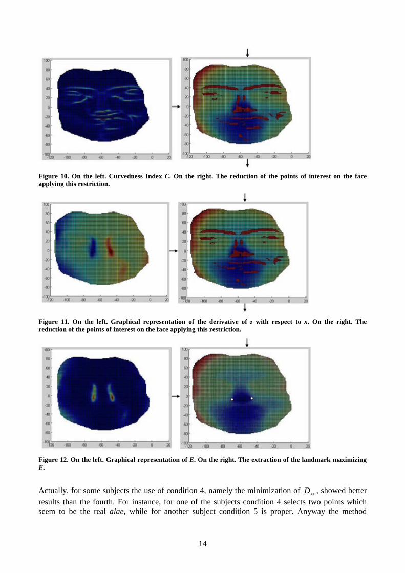
Figure 10. On the left. Curvedness Index C. On the right. The reduction of the points of interest on the face applying this restriction.

Figure 11. On the left. Graphical representation of the derivative of z with respect to x. On the right. The reduction of the points of interest on the face applying this restriction.

Figure 12. On the left. Graphical representation of E. On the right. The extraction of the landmark maximizing E.

Actually, for some subjects the use of condition 4, namely the minimization of xxD , showed better results than the fourth. For instance, for one of the subjects condition 4 selects two points which seem to be the real alae, while for another subject condition 5 is proper. Anyway the method

15

employing condition 5 was chosen as “official method”, because its overall results on the thirty clouds were the most satisfactory. 3.4 Endocanthions

The localization of the endocanthions was performed firstly selecting the points whose Shape Index lies in the range corresponding to the surfaces of cup and rut, then choosing among these points the critical ones, because in the reference system employed they are local maximums. The derivative of z with respect to x is positive on the right endocanthion and negative on the left, the second derivative of z with respect to x is negative in them, and both the Coefficients f and F are negative on the right EN and positive on the left. After selecting the zones of interest, the extraction is completed minimizing e.

Figure 13. On the left. The points whose Shape Index lies in the range corresponding to the surface of cup, in blue. On the right. The reduction of the points of interest on the face applying this restriction.

Figure 14. On the left. Critical points, in blue. On the right. The reduction of the points of interest on the face applying this restriction.

16

Figure 15. On the left. Graphical representation of the first derivative of z with respect to x. On the right. The reduction of the points of interest on the face applying this restriction.

Figure 16. On the left. Graphical representation of he second derivative of z with respect to x. On the right. The reduction of the points of interest on the face applying this restriction.

Figure 17. On the left. Graphical representation of f. On the right. The reduction of the points of interest on the face applying this restriction.

17

Figure 18. On the left. Graphical representation of F. On the right. The reduction of the points of interest on the face applying this restriction.

Figure 19. On the left. Graphical representation of e. On the right. The extraction of the landmark minimizing e.

Similarly to the outer corners of eyes, the exocanthions, they are not easily extractable, namely the elaboration of the algorithm was not immediate. The reason is that eyes may be open or close, and their geometrical features differ a little bit in the two situations. For instance, during the scanning, two subjects kept their eyes closed, while the other four subjects kept them open for all their scans. The aim was to implement only one algorithm, and so it was did, but the results are not as accurate as for the other landmarks. The localization of the areas of interest are right, but the extraction of the two landmarks is not rigorous for all the faces. Furthermore, it was necessary to localize the areas of landmarks through the coordinates of PN.

Furthermore the localization was not accurate for all the scans because, unlike the other points, no descriptors have a local maximum or minimum in them. The eyes are a moving part of the face, so it is not easy to describe their geometry precisely. 3.5 Exocanthions

The exocanthions were localized selecting the points whose Shape Index lies in the range corresponding to the surface of ridge, choosing among them the points whose first derivative of z with respect to x is positive in the right exocanthion and negative in the left, and whose second derivative with respect to y is positive. Then the points in which g is positive, F is negative in the right EX and positive in the left, and K is positive or equal to zero in them where selected. The point of reference was extracted maximizing E.

18

Figure 20. On the left. The points whose Shape Index lies in the range corresponding to the surface of ridge, in red. On the right. The reduction of the points of interest on the face applying this restriction.

Figure 21. On the left. Graphical representation of the derivative of z with respect to x. On the right. The reduction of the points of interest on the face applying this restriction.

Figure 22. On the left. Graphical representation of the second derivative of z with respect to y. On the right. The reduction of the points of interest on the face applying this restriction.

19

Figure 23. On the left. Graphical representation of g. On the right. The reduction of the points of interest on the face applying this restriction.

Figure 24. On the left. Graphical representation of F. On the right. The reduction of the points of interest on the face applying this restriction.

Figure 25. On the left. Graphical representation of K. On the right. The reduction of the points of interest on the face applying this restriction.

20

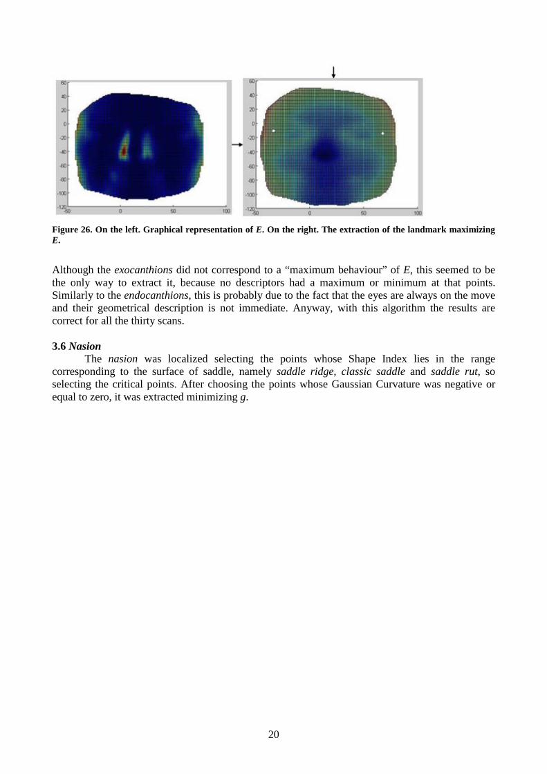
Figure 26. On the left. Graphical representation of E. On the right. The extraction of the landmark maximizing E.

Although the exocanthions did not correspond to a “maximum behaviour” of E, this seemed to be the only way to extract it, because no descriptors had a maximum or minimum at that points. Similarly to the endocanthions, this is probably due to the fact that the eyes are always on the move and their geometrical description is not immediate. Anyway, with this algorithm the results are correct for all the thirty scans. 3.6 Nasion The nasion was localized selecting the points whose Shape Index lies in the range corresponding to the surface of saddle, namely saddle ridge, classic saddle and saddle rut, so selecting the critical points. After choosing the points whose Gaussian Curvature was negative or equal to zero, it was extracted minimizing g.

21

Figure 27. On the left. The points whose Shape Index lies in the range corresponding to the surface of saddle ridge, the coloured ones. On the right. The reduction of the points of interest on the face applying this restriction.

Figure 28. On the left. Critical points, in red. On the right. The reduction of the points of interest on the face applying this restriction.

22

Figure 29. On the left. Graphical representation of K, also shown in another view. On the right. The reduction of the points of interest on the face applying this restriction.

Figure 30. On the left. Graphical representation of g, in two views. On the right. The extraction of the landmark minimizing g.

23

Since it has no significant changes of curvature, it has been very hard to extract it, although it has not many geometrical conditions. Coefficient g plays an important rule. Its “minimum behaviour” was not theoretically obvious and a deep study of the generated graphs was necessary. Nevertheless, this feature was not evident in all the scans, so before this discover it seemed to be impossible to find the nasion. After a targeted analysis of the graphs this behaviour of g was realized and then the extraction of the landmark was immediate and accurate. It should be considered it a strong result, probably the best of this paper. 4. Discussion and conclusions

The resulting nine landmarks of nine of the thirty faces are shown in Figure 31. The table in Figure 32 summarizes the coordinates obtained of all the landmarks of ten faces.

Figure 31. The extracted landmarks for nine of the thirty faces.

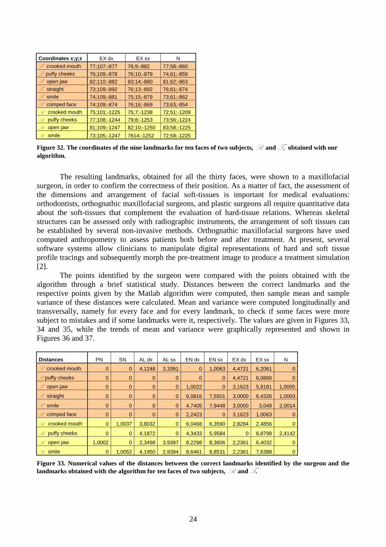
Coordinates x;y;z SN AL dx AL sx F crooked mouth 45;61;-846 53;71;-847 51;49;-849 F puffy cheeks 42;60;-852 49;71;-854 49;50;-854 F open jaw 46;62;-860 54;73;-856 54;53;-855 F straight 43;61;-866 50;73;-862 50;51;-863 F smile 40;62;-861 48;74;-856 48;52;-857 F crimped face 43;63;-849 52;75;-847 53;51;-847 B crooked mouth 40;51;-1203 48;59;-1200 47;39;-1206 B puffy cheeks 42;55;-1216 51;65;-1216 51;43;-1221 B open jaw 46;57;-1216 55;67;-1213 55;47;-1216 B smile 42;58;-1219 53;65;-1213 52;47;-1216

24

Coordinates x;y;z EX dx EX sx N F crooked mouth 77;107;-877 76;9;-882 77;58;-860 F puffy cheeks 76;109;-878 76;10;-879 74;61;-859 F open jaw 82;110;-882 83;14;-880 81;62;-863 F straight 73;109;-892 76;13;-892 76;61;-874 F smile 74;109;-881 75;15;-879 73;61;-862 F crimped face 74;109;-874 76;16;-869 73;63;-854 B crooked mouth 75;101;-1225 75;7;-1238 72;51;-1209 B puffy cheeks 77;108;-1244 79;8;-1253 73;56;-1224 B open jaw 81;109;-1247 82;10;-1250 83;58;-1225 B smile 73;105;-1247 7614;-1252 72;58;-1225

Figure 32. The coordinates of the nine landmarks for ten faces of two subjects, B and F, obtained with our algorithm.

The resulting landmarks, obtained for all the thirty faces, were shown to a maxillofacial

surgeon, in order to confirm the correctness of their position. As a matter of fact, the assessment of the dimensions and arrangement of facial soft-tissues is important for medical evaluations: orthodontists, orthognathic maxillofacial surgeons, and plastic surgeons all require quantitative data about the soft-tissues that complement the evaluation of hard-tissue relations. Whereas skeletal structures can be assessed only with radiographic instruments, the arrangement of soft tissues can be established by several non-invasive methods. Orthognathic maxillofacial surgeons have used computed anthropometry to assess patients both before and after treatment. At present, several software systems allow clinicians to manipulate digital representations of hard and soft tissue profile tracings and subsequently morph the pre-treatment image to produce a treatment simulation [2].

The points identified by the surgeon were compared with the points obtained with the algorithm through a brief statistical study. Distances between the correct landmarks and the respective points given by the Matlab algorithm were computed, then sample mean and sample variance of these distances were calculated. Mean and variance were computed longitudinally and transversally, namely for every face and for every landmark, to check if some faces were more subject to mistakes and if some landmarks were it, respectively. The values are given in Figures 33, 34 and 35, while the trends of mean and variance were graphically represented and shown in Figures 36 and 37.

Distances PN SN AL dx AL sx EN dx EN sx EX dx EX sx N

F crooked mouth 0 0 4,1248 3,3391 0 1,0063 4,4721 6,2061 0

F puffy cheeks 0 0 0 0 0 0 4,4721 6,0890 0 F open jaw 0 0 0 0 1,0022 0 3,1623 5,8181 1,0005

F straight 0 0 0 0 6,0816 7,5501 3,0000 6,4326 1,0003

F smile 0 0 0 0 4,7405 7,9448 3,0000 3,049 2,0014 F crimped face 0 0 0 0 2,2423 0 3,1623 1,0063 0

B crooked mouth 0 1,0037 3,8032 0 6,0468 6,3590 2,8284 2,4856 0

B puffy cheeks 0 0 4,1872 0 4,3433 5,9584 0 6,8798 2,4142

B open jaw 1,0002 0 2,3498 3,9397 8,2298 8,3606 2,2361 6,4032 0

B smile 0 1,0052 4,1950 2,9394 8,6461 8,8531 2,2361 7,6388 0

Figure 33. Numerical values of the distances between the correct landmarks identified by the surgeon and the landmarks obtained with the algorithm for ten faces of two subjects, B and F.

25

Mean and variance mean variance

F crooked mouth 2,1276 5,869

F puffy cheeks 1,1735 5,5854

F open jaw 1,2203 4,0566

F straight 2,6739 10,1280

F smile 2,3040 7,5149 F crimped face 0,7123 1,4342

B crooked mouth 2,5030 6,2833 B puffy cheeks 2,6425 7,7765

B open jaw 3,6133 11,0216

B smile 3,9460 12,9496

Figure 34. Values of sample mean and sample variance computed between the nine landmarks for ten faces of two subjects, B and F.

Mean and variance PN SN AL dx AL sx AL EN dx EN sx EN EX dx EX sx EX N

mean 0,1000 0,2009 1,8660 1,0218 1,4439 4,1333 4,6032 4,3682 2,8569 5,2009 4,0289 0,6416

variance 0,1000 0,1794 4,1457 2,7633 3,2727 10,31 13,4389 11,2492 1,5895 3,0473 2,1964 0,8262

Figure 35. Values of sample mean and sample variance computed between the ten faces for the nine landmarks. Mean and variance were calculated between the faces. Next to the right and left values of alae, endocanthions and exocanthions, another value is given, identified by the abbreviations AL, EN and EX. These values were obtained involving both the data of the right and the left landmark, i.e. averaging among twenty faces.

Figure 36. Graphical representation of the values of sample mean and sample variance computed between the nine landmarks for ten faces of two subjects, B and F.

26

Figure 37. Graphical representation of values of sample mean and sample variance computed between the ten faces for the nine landmarks.

The localization seems to be quite accurate on face soft-tissues. The first graph shows that

some faces are less subject to mistakes than others, for instance F’ ‘s puffy cheeks, F’ ‘s open jaw and F’ ‘s crimped face, while other faces are more subject to mistakes, i.e. F’ ‘s straight expression, B ‘s open jaw and B ‘s smile. It may be due to the fact the some poses on different people can change their faces a lot. The values of the other graph show that the position of the endocanthions was not as accurate as that of all the other landmarks in all the faces, although the area of interest was correctly identified. The landmarks which were best positioned are surely the pronasal, the subnasal and the nasion: their sample mean and variance values are approximately equal to zero. The distances between the landmarks are partially equal to zero, while the ones with the highest values are recorded for the endocanthions and exocanthions, reaching a maximum of 8.8531, although their areas of interest was correctly localized. The results are very good, if the fact that the extraction was only geometrical is considered. As described above, facial surface is a particular free-form surface, constituted by intersected and overlapped different patches. Each face is unique but its features are the same for all mankind. This allows to use the face as an instrument for recognition and identification.

Differential Geometry gave the research the possibility to describe facial features through landmarks, which are known worldwide by aesthetic plastic surgeons and face recognition companies. A geometric profile of each landmark that has noticeable feature, gives no identification problem and is far from the areas of face that are more subject and influenced by facial expressions, such as the mouth, is here provided. The fact is that these points were not only accurately describable, but even suitable to a geometrical description. Furthermore, their localization in the face was quite accurate. In fact, the results obtained here were shown to an expert, a maxillofacial surgeon, who confirmed their correctness. So, the Matlab algorithm elaborated for the landmarks extraction holds for the thirty faces and works correctly for all of them.

A future work should deepen the mathematical study of these and other landmarks. Moreover, the computed three-dimensional distances between landmarks shown in the last chapter could be used to verify computationally, through a focused algorithm, that a face recognition is really possible only using geometry.

27

5. References

[1] ALKER, M., FRANTZ, S., ROHR, K. AND STIEHL, H. S. (2001) “Improving the Robustness in Extracting 3D Point Landmarks from 3D Medical Images Using Parametric Deformable Models”, Springer-Verlag, 582-590.

[2] CALIGNANO, F. (2009) Morphometric methodologies for bio-engineering applications, PhD Degree Thesis, Politecnico di Torino, Department of Production Systems and Business Economics.

[3] D’HOSE, J., COLINEAU, J., BICHON, C. AND DORIZZI, B. (2007) “Precise Localization of Landmarks on 3D Faces using Gabor Wavelets”, First IEEE International Conference on Biometrics: Theory, Applications, and Systems, 1-6.

[4] FRANTZ, S., ROHR, K. AND STIEHL, H. S. (1998) “Multi-Step Procedures for the Localization of 2D and 3D Point Landmarksand Automatic ROI Size Selection”, Springer-Verlag, Vol.I: 687-703.

[5] FRANTZ, S., ROHR, K. AND STIEHL, H. S. (1999) “Improving the Detection Performance in Semi-automatic Landmark Extraction”, Springer-Verlag, 253-263.

[6] FRANTZ, S., ROHR, K. AND STIEHL, H. S. (2000) “Localization of 3D Anatomical Point Landmarks in 3D Tomographic Images Using Deformable Models”, Springer-Verlag, 492-501.

[7] FRANTZ, S., ROHR, K. AND STIEHL, H. S. (2005) “Development and validation of a multi-step approach to improved detection of 3D point landmarks in tomographic images”, Science Direct, 23: 956-971.

[8] KOENDERINK, J. J. AND VAN DOORN, A. J. (1992) “Surface shape and curvature scales”, Image and Vision Computing, 10(8): 557-564.

[9] ROMERO, M. AND PEARS, N. (2009) “Landmark Localisation in 3D Face Data”, 6th IEEE International Conference on Advanced Video and Signal Based Surveillance, 73-78.

[10] ROMERO, M. AND PEARS, N. (2009) “Point-pair descriptors for 3D facial landmark localisation”, IEEE 3rd International Conference on Biometrics: Theory, Applications, and Systems, 1-6.

[11] RUIZ, M. C. AND ILLINGWORTH, J. (2008) “Automatic landmarking of faces in 3D - ALF3D”, 5th International Conference on Visual Information Engineering - IEEE Conferences, 41-46.

[12] SALAH, A. A. AND AKARUN, L. (2006) “Gabor Factor Analysis for 2D+3D Facial Landmark Localization”, IEEE 14th Signal Processing and Communications Applications, 1-4.

[13] SANG-JUN, P. AND DONG-WON, S. (2008) “3D face recognition based on feature detection using active shape models”, International Conference on Control, Automation and Systems - IEEE Conferences, 1881-1886.

[14] WÖRZ, S. AND ROHR, K. (2005) “Localization of anatomical point landmarks in 3D medical images by fitting 3D parametric intensity models”, Science Direct, 10: 41-58.

[15] CYBERWARE COLOR 3D DIGITIZER PRODUCT INFORMATION. CYBERWARE INC. MONTEREY CA, USA.