Bregman Iterative Algorithms for 2D

Geosounding Inversion

Hugo Hidalgo-Silva Email: hugo@cicese.mx and E. Gomez-Trevino.

CICESE,Carr. Ensenada-Tijuana no. 3918

Ensenada, Baja California 22860 Mexico.

January 22, 2015

Abstract

Bregman iterative algorithms have been extensively used for l1 andTV regularization problems, allowing to obtain simple, fast and effec-tive algorithms. In this paper, three already available algorithms forgeosounding inversion are modified by including them in a Bregmaniterative procedure. The resulting algorithms are easy to implementand do not require any optimization package. Modeling results arepresented for synthetic and field data, observing better convergenceproperties than the original versions, avoiding the need of any contin-uation descent procedure.

1 Introduction

Tikhonov’s regularization method [1] is the standard technique applied toobtain models of the subsurface conductivity distribution from electric orelectromagnetic measurements (e.g. [2, 3]). The model proposed for theconductivity distribution (m) is obtained by minimizing the functional

UT (m) = ‖F (m)− d‖2H + λP (m). (1)

1

In this formulation, F :M⊃ D(F)→ H represents the direct functional,applied to an element on the model space M, a Banach space and return-ing a member of the Hilbert space H of data. The second term correspondto the Tikhonov’s stabilizing functional, with P (m) = ‖∇m‖2M, maximumsmoothness functional the usual approach [3, 4, 5] and λ the regularizationparameter, controlling the trade-off between smoothness of the model andgoodness of fit to the data. Due to the roughness penalizer inclusion, themodel developed by Tikhonov’s algorithm tends to smear discontinuities,a feature that may be undesirable in situations where different rock typessimply face each other without a fuzzy transition. In an effort to generatemodels with sharp boundaries, several techniques have been applied to thisproblem: piecewise continuous formulations as in [6, 7, 8], l1 norm minimiza-tion [9, 10, 11], total variation penalizers in [13] and [14], among others.

In this work, we will consider the discrete version of linear problemF (m) =

∫∞0

∫∞−∞ κ(x, z)m(x, z)dxdz, with κ the kernel of a Fredholm integral

equation of the first kind,

U(m) = ‖Am− d‖2 + λP (m) (2)

with A the matrix of integral kernel evaluations, and P (m) the discreteversion of stabilizing operator.

For the total variation (TV) approach the reconstruction problem is for-mulated with the stabilizing functional PTV (m) =

∫

|∇m|, with |∇m| =√

(∂m∂x

)2 + (∂m∂z

)2 for a two-dimensional model.

The non-differentiability of the Euclidean norm at the origin complicatesthe minimization procedure, and a smooth approximation like P θ

TV (m) =∫

h(|∇m|), with h(|∇m|) =√

(∂m∂x

)2 + (∂m∂z

)2 + θ2 is usually considered in

practice. The small positive parameter θ is incorporated in order to stabilizethe numerical algorithm [16].

Minimization of (2) with PTV was at first implemented by constructingthe Euler-Lagrange equations and then performing an iterative procedurebased on half-quadratic regularization. In practice, the construction had todeal with severe conditioning problems [14, 16].

Several improvements to TV that do not incorporated the parameter θwere proposed later [17, 18]. Among them, the introduction of hybrid regu-larization operators that consist of a sum of PTV (·) and other Pα(·) are usedto stabilize the algorithm [17]. Ordinarily, the hybrid regularizer maintains

2

the combination of operators constant during optimization. In practice, TVtends to produce low-contrasted solutions, and in the case of integral equa-tions with a slow-decaying kernel, smooth, staircase type models. Severalenhanced versions of TV have been developed by applying Bregman itera-tions [15, 20]. The models developed by the Bregman versions present highercontrast, but the staircasing effect remains for the slow-decaying kernel in-verse problems.

Observing the TV limitations, particularly for geosounding inversion,Portniaguine and Zhdanov [5] proposed the Minimum Support (MS) andMinimum Gradient Support (MGS) stabilizing functionals in order to de-velop models with sharp boundaries. The stabilizing functional they intro-duced minimize the area where significant variations of the model parametersand/or discontinuities occur.

The nonlinear functional is minimized by considering a reweighted least-squares iterative procedure applying conjugate gradient descent.

A Bregman version of the algorithm is presented here for electromagneticsounding data, applying Barzilai-Borwein algorithm to obtain the inner so-lution of a quadratic problem.

As observed below, a modified version can be obtained considering everycoordinate separately, and a Line-Process [6] type algorithm results. Theregularization functional corresponds to the edge-preserving operator (EPR)[39], a Bregman version of this algorithm is also presented here.

A hybrid regularization method is proposed in [19], implementing ho-motopy continuation in order to move from a smooth enhancing (L2) to adiscontinuous-preserving (L1) operator. The optimization is realized with acoordinate gradient descent (CGD) based numerical method. In this paper,a Bregman iteration version of the algorithm is presented, relieving the needfor continuation and presenting better convergence properties.

Bregman iterative regularization was introduced by Osher et. al. [20] inimage processing. They extended the Rudin-Osher-Fatemi [21] model

minu

λ

∫

|∇u|+ 1

2‖u− b‖2 (3)

in which u is an unknown image, b is an input noisy measurement of aclean image u, and λ the regularization parameter, into an iterative regular-ization model by using the Bregman distance based on the total variationfunctional J(u) = λPTV (u) = λ

∫

|∇u|.

3

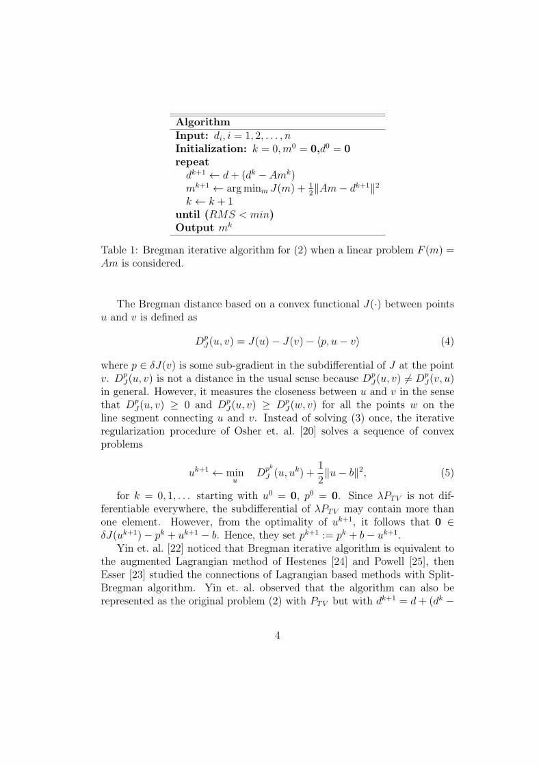
AlgorithmInput: di, i = 1, 2, . . . , nInitialization: k = 0,m0 = 0,d0 = 0repeatdk+1 ← d+ (dk − Amk)mk+1 ← argminm J(m) + 1

2‖Am− dk+1‖2

k ← k + 1until (RMS < min)Output mk

Table 1: Bregman iterative algorithm for (2) when a linear problem F (m) =Am is considered.

The Bregman distance based on a convex functional J(·) between pointsu and v is defined as

DpJ(u, v) = J(u)− J(v)− 〈p, u− v〉 (4)

where p ∈ δJ(v) is some sub-gradient in the subdifferential of J at the pointv. Dp

J(u, v) is not a distance in the usual sense because DpJ(u, v) 6= Dp

J(v, u)in general. However, it measures the closeness between u and v in the sensethat Dp

J(u, v) ≥ 0 and DpJ(u, v) ≥ Dp

J(w, v) for all the points w on theline segment connecting u and v. Instead of solving (3) once, the iterativeregularization procedure of Osher et. al. [20] solves a sequence of convexproblems

uk+1 ← minu

Dpk

J (u, uk) +1

2‖u− b‖2, (5)

for k = 0, 1, . . . starting with u0 = 0, p0 = 0. Since λPTV is not dif-ferentiable everywhere, the subdifferential of λPTV may contain more thanone element. However, from the optimality of uk+1, it follows that 0 ∈δJ(uk+1)− pk + uk+1 − b. Hence, they set pk+1 := pk + b− uk+1.

Yin et. al. [22] noticed that Bregman iterative algorithm is equivalent tothe augmented Lagrangian method of Hestenes [24] and Powell [25], thenEsser [23] studied the connections of Lagrangian based methods with Split-Bregman algorithm. Yin et. al. observed that the algorithm can also berepresented as the original problem (2) with PTV but with dk+1 = d+ (dk −

4

Amk) as input, instead of d, obtaining the ‘add-back residual’ version:

mk ← solve (2) with d := dk (6)

dk+1 ← d+ (dk − Amk). (7)

The Bregman iterative algorithm applied to (2) is presented on Table 1. Aconvergence termination criteria is established when fitness to data (RMS =1√N‖d − Am‖) reaches some minimum, with A the matrix containing the

discrete evaluation of the kernel κ. Osher et. al. [20] presented convergenceresults when H(m) generalizes the data fitness term 1

2‖Am − d‖22. They

showed that a sequence {mk} of Bregman iterations (6,7) has the followingproperties:

1. Monotonic decrease in H(·): H(mk+1) ≤ Dpk

J (mk+1,mk) +H(mk+1) ≤H(mk).

2. Convergence to the true solution m∗ in H with exact data: if m∗ mini-mizes H(·) and satisfies J(m∗) <∞, then H(mk) ≤ H(m∗)+J(m∗)/k.

3. Convergence to m∗ in D with noisy data: Let H(·) = H(·; d) and mobeys H(m, d) ≤ δ and H(m, d0) = 0, with d, d0, m, and δ representingthe noisy input, noiseless input, true signal and noise level, respectively.

Then Dpk+1

j (m,mk+1) < Dpk

j (m,mk), for k obeying H(mk+1, d) > δ.

Recently, Yin and Osher [26] observed the so called ‘error forgetting’ prop-erty of add-back Bregman iterations (6,7) when applied to convex piece-wiselinear functions J(·). When wk denotes the numerical error at iteration k of(6), if all wk are sufficiently small so that Bregman iteration identifies theoptimal face of the solution polyhedra, then the distance between the cur-rent point mk and the optimal solution set M∗ is bounded by ‖wk+1 − wk‖,independently of the numerical errors of previous iterations. This propertyallows to construct optimization algorithms with better convergence perfor-mance than their original non Bregman versions. Bregman iterations wereproposed for convex, non-differentiable problems. The three inversion algo-rithms mentioned before (MGS, EPR and CGD) are modified to include aBregman iteration and presented on section 3 for the 2D geosounding method.Optimization with the augmented Lagrangian method has been applied togeosciences [27, 28, 29] before. A Split Bregman iterative algorithm was ap-plied to the reconstruction of electrical impedance tomography by Wang et.

5

al. [30]. An application of Bregman iteration with Barzilai-Borwein optimiza-tion to a inverse problem is presented by Ma in [31]. To the authors’ bestknowledge, exception made for a recent congress [32], Bregman iterationshave not been considered for geosounding inversion before.

2 The 2D Geosounding Problem

To investigate the internal structure of the earth, geophysicists rely mostlyon the interpretation of measurements taken on the surface. This applies fordeep soundings of hundreds of kilometers as for shallow studies of merely afew meters below the surface. The electrical conductivity of rocks is oftenthe property of interest in these type of studies. For this reason, a greatamount of electrical techniques have been developed to infer the conductivitystructure of the subsurface on the basis of surface measurements.

One of these techniques is based on electromagnetic induction by meansof an alternating current that is made to flow in a transmitting coil. This cur-rent generates an alternating magnetic field in the surrounding environment,which in turn induces an electromotive force in a receiving coil e.g. [33]. Aparticular version that works at low induction numbers is of special interestfrom both theoretical and practical reasons. We exploit here the peculiartheoretical aspect of the technique. In 1D the surface measurements can beexactly represented by a linear functional of the unknown conductivity of thesubsurface e.g. [35]. In two dimensions (2D), the corresponding functionalis necessarily nonlinear [36], but it can be approximated for many practicalapplications using a linear functional [37]. Apparent conductivity σa, a nor-malized version of the measurements, can be expressed for a 2D conductivitydistribution σ(x, z) as:

σa =2|x2 − x1|

π

∫ ∞

0

∫ ∞

−∞A2D(x, z, x1, x2)σ(x, z)dxdz, (8)

where A2D is, for vertical dipoles:

A2D(x, z, x1, x2) =

∫ ∞

0

(y2 − (x− x1)(x2 − x))dy√

[(r21 + z2]3[r22 + z2]3, (9)

and for horizontal dipoles:

A2D(x, z, x1, x2) =

∫ ∞

0

(Ex1Ex2 + Ey1Ey2)dy, (10)

6

with

Ey1 = y(x− x1)(

2

r41− 2z

r41√

r21 + z2− z

r21(r21 + z2)3/2

)

,

Ey2 = y(x− x2)(

2

r42− 2z

r42√

r22 + z2− z

r22(r22 + z2)3/2

)

,

Ex1 =

[

1

r21− z

r21√

r21 + z2− 2y2

r41+

y2z

r21(r21 + z2)3/2

+2y2z

r41√

r21 + z2

]

,

Ex2 =

[

1

r22− z

r22√

r22 + z2− 2y2

r42+

y2z

r22(r22 + z2)3/2

+2y2z

r42√

r22 + z2

]

,

x1 is the location of the transmitting coil, x2 the location of the receivingcoil, r1 =

√

(x− x1)2 + y2 and r2 =√

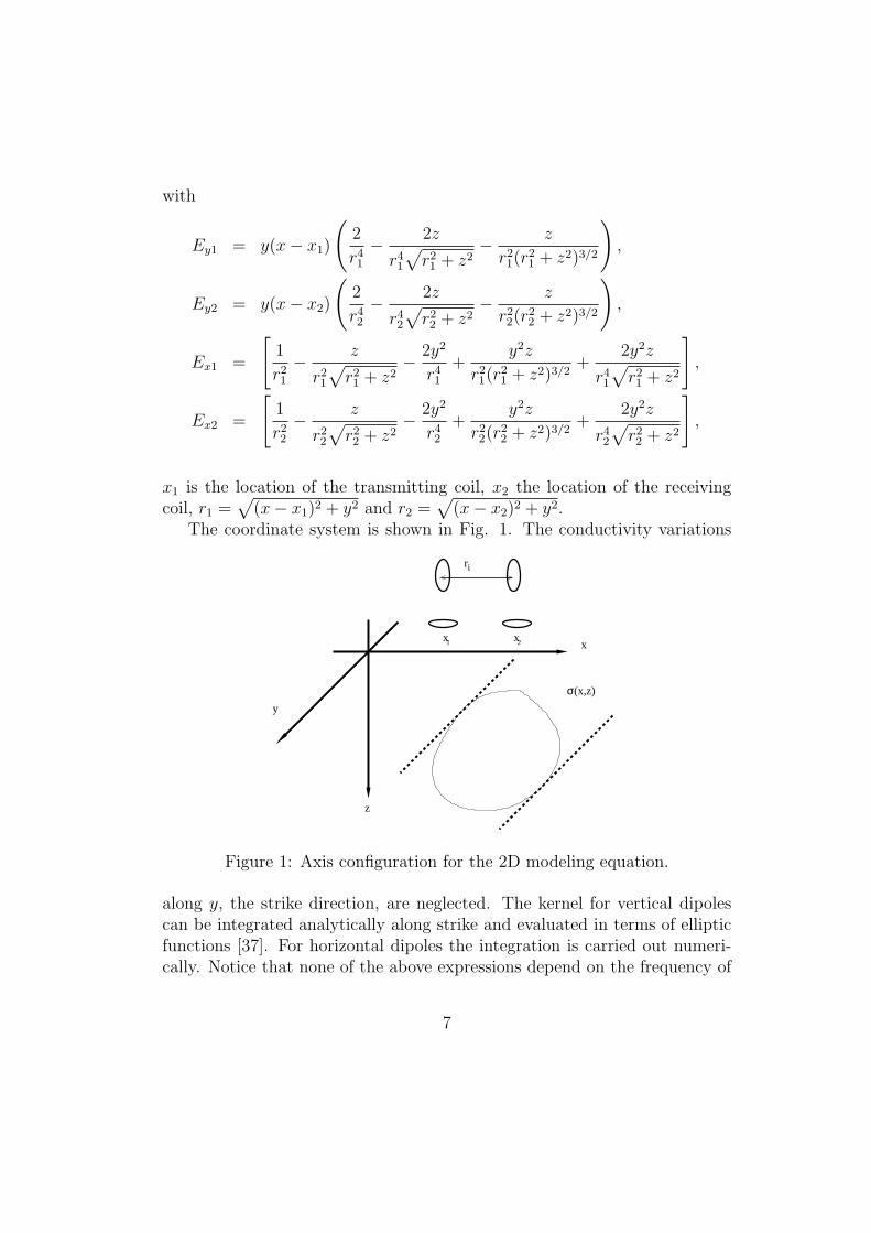
(x− x2)2 + y2.The coordinate system is shown in Fig. 1. The conductivity variations

y

σ(x,z)

x

ri

z

1x x2

Figure 1: Axis configuration for the 2D modeling equation.

along y, the strike direction, are neglected. The kernel for vertical dipolescan be integrated analytically along strike and evaluated in terms of ellipticfunctions [37]. For horizontal dipoles the integration is carried out numeri-cally. Notice that none of the above expressions depend on the frequency of

7

the electromagnetic field. The depth of penetration of electromagnetic mea-surements at low induction numbers is independent of frequency. In fact,the induced currents in the ground are proportional to frequency, and so arethe associated fields and therefore the measurements. However, because thenormalization factors derived from the responses of a homogeneous mediumare also proportional to frequency, the final expressions are frequency in-dependent [41]. More practical way is to pose the problem as a system oflinear equations with many unknown values of the conductivity distribution.Since the number of unknowns is usually much larger than the number ofequations, some kind of regularization is required. At the same time, it isdesirable that the solution resembles a layered earth with distinct bordersthat separate a few zones of uniform conductivity, regardless of the numberof unknowns.

3 Bregman Iterative Algorithms

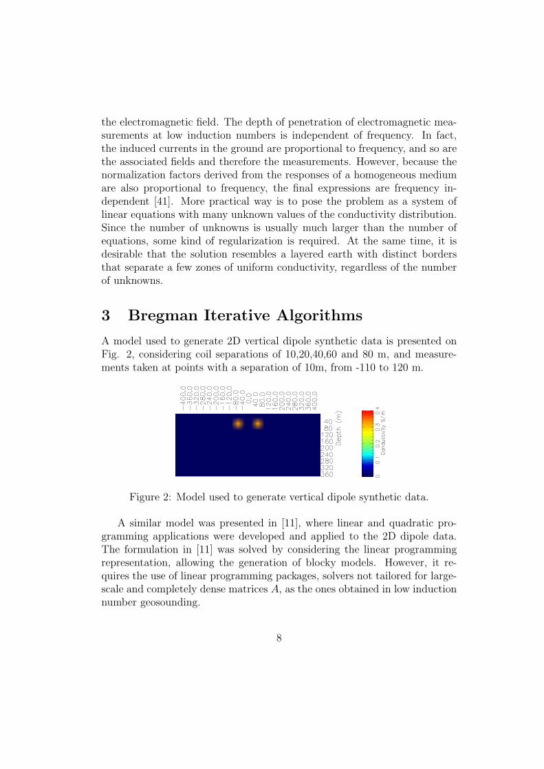
A model used to generate 2D vertical dipole synthetic data is presented onFig. 2, considering coil separations of 10,20,40,60 and 80 m, and measure-ments taken at points with a separation of 10m, from -110 to 120 m.

Figure 2: Model used to generate vertical dipole synthetic data.

A similar model was presented in [11], where linear and quadratic pro-gramming applications were developed and applied to the 2D dipole data.The formulation in [11] was solved by considering the linear programmingrepresentation, allowing the generation of blocky models. However, it re-quires the use of linear programming packages, solvers not tailored for large-scale and completely dense matrices A, as the ones obtained in low inductionnumber geosounding.

8

3.1 Minimum Gradient Support

The minimum gradient support functional is defined as [5]

PMGS(m) =

∫

V

∇m · ∇m∇m · ∇m+ β2

dv, (11)

with β a small positive constant. As observed by Portniaguine and Zhdanov,PMGS can be treated as a functional proportional (for a small β) to thegradient support, helping to generate a sharp and focused model.

A procedure to select β based on a initial minimum norm model is pre-sented on [12]. Application of minimum gradient support functional to thelinear EM geosounding represents the solution of a nonlinear, non convexinverse problem. Portniaguine and Zhdanov consider a quadratic approxi-mation for it, the solution of

UMGS = (Am− d)t(Am− d) + λ(Wem)tWem, (12)

with We a weighting matrix implementing the weighting function we(m) =∇m

(∇m·∇m+β2)1/2in a reweighted conjugate-gradient least squares formulation

[5]. A problem with this technique is that a zero or small constant initialmodel will produce a zero in the Frechet derivative, making difficult for theconjugate gradient to move out of the initial model. They use as startingmodel a minimum norm solution to overcome this problem.

An iterative algorithm is easily obtained incorporating J(m) = λ(Wem)tWemin algorithm 1. The minimization step can be implemented with a box-constrained Barzilai-Borwein procedure, that present better convergence prop-erties than conjugate-gradient [38]. The box restrictions are incorporated toavoid useless negative solutions, and may be stated considering the mea-surements. It should be observed that for this kernel we may have negativemeasurements, so the lower bound should be a small near zero value. Theupper bound can be considered as ten times the maximum measurement.

A model developed after applying synthetic data obtained from model inFigure 2 is presented on Figure 3. The model was obtained after 11 iterationsof Bregman iterative algorithm with λ = 0.01, β = 0.01 and halted whenRMS ≤ 0.002.

After numerical experimentation, it was observed that only five inneriterations for the Barzilai-Borwein procedure were required for convergence.Also, a uniform initial model m0 = 0.001 was used, instead of the minimumnorm solution. Regularization parameter λ is determined from the misfit

9

condition ‖Amλ − d‖ = ǫ, where ǫ is some a priori estimation of noise levelof the data. By applying the procedure proposed by Zhdanov and Tolstaya[12], β would be among [0.01, 0.04]. Due to the operator nature, a smallβ would produce compact, blocky models, but tends to obscure the lesscontrasted parts of the model. The original algorithm without the Bregmanresidual error update would not converge for this parameters. A lower λ of0.001 and a initial model given by the minimum norm solution would haveto be considered.

Figure 3: Model developed by Bregman iterative algorithm with the MGSoperator with Barzilai-Borwein optimization in the inner step for the samesynthetic data of model in Figure 2.

3.2 Edge Preserving Regularization

The weighted least-squares procedure implemented on the MGS algorithmwas necessary to avoid the direct minimization of the resulting nonlinearoperator equation. Now, consider the following split version of the MGSoperator

PMGSSplit(m) =

∫

(Dxm)2

(Dxm)2 + β2dx+

∫

(Dzm)2

(Dzm)2 + β2dz, (13)

with Dxm = ∂m∂x

, Dzm = ∂m∂z

. This operator has been considered onthe vision community under the name of “edge-preserving regularization”(EPR) [39], and applied to the resistivity inverse problem by Hidalgo et. al.in [40]. Charbonnier et. al. proposed to minimize the inverse problem withEPR operator

PEPR =∑

k

φ[(Dxm)k] +∑

k

φ[(Dzm)k] (14)

10

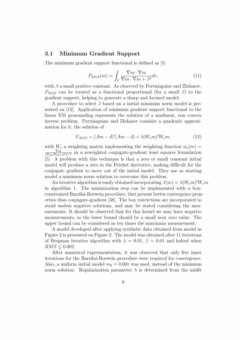
where (Dxm)k is the finite difference implementation of first-order derivativeat point k, and φ is the potential function. They developed some propertiesthat a potential function has to comply in order to obtain an edge-preservingregularization operator. As can be observed from [39], operator (13) is con-sidered by Charbonnier et. al. as the Geman-McClure potential function,when β = 1. They proposed to apply an iterative algorithm called “halfquadratic regularization” for the minimization of a modified version of theoriginal functional (2) with P = PEPR. The algorithm is aimed to minimizethe dual functional

U∗EPR(m, bx, bz) = ‖Am− d‖2 + λ

∑

k

φ∗[(Dx)k, (bx)k] + λ∑

k

φ∗[(Dz)k, (bz)k]

(15)with φ∗ defined such that φ(t) = infw φ

∗(t, w), and bx, bz auxiliary variablesintroduced to ease the minimization of the augmented energy functional

U∗EPR(m, bx, bz) = ‖Am− d‖2 + λ

∑

k

(bx)k(Dxm)2k + ψ[(bx)k]

+ λ∑

k

(bz)k(Dzm)2k + ψ[(bz)k]. (16)

ψ is a strictly convex and decreasing function such that φ(t) = infw(wt2 +

ψ(w)), and for the case of operator in (13), ψ(w) = wβ2 − 2√wβ + 1.

The half quadratic procedure is based on alternating minimizations overm and b. Charbonnier et. al. proved convergence of this procedure when φ(t)possess the edge-preserving conditions [39]. The convexity of ψ allows toeasily incorporate the half quadratic minimization in the Bregman algorithm1, observing that, in a coordinate descent algorithm, the minimum for rthelement of m is

mr =

∑

j djajr + λ[mr−nx(bz)r +mr+nx(bz)r+nx +mr−1(bx)r +mr+1(bx)r+1]∑

j a2jr + λ((bz)r + (bz)r+nx) + (bx)r + (bx)r+1

,

(17)and the minimum for b is at

(bz)r =φ′(mr −mr−nx)

2(mr −mr−nx), (18)

(bx)r =φ′(mr −mr−1)

2(mr −mr−1). (19)

11

With aij = [A]ij , and considering m as a vector representation of a 2Dmodel with nx elements in x coordinate.

As before, a Bregman iterative procedure is obtained easily, by using(17,18), and (19) to solve the minimization step for mr.

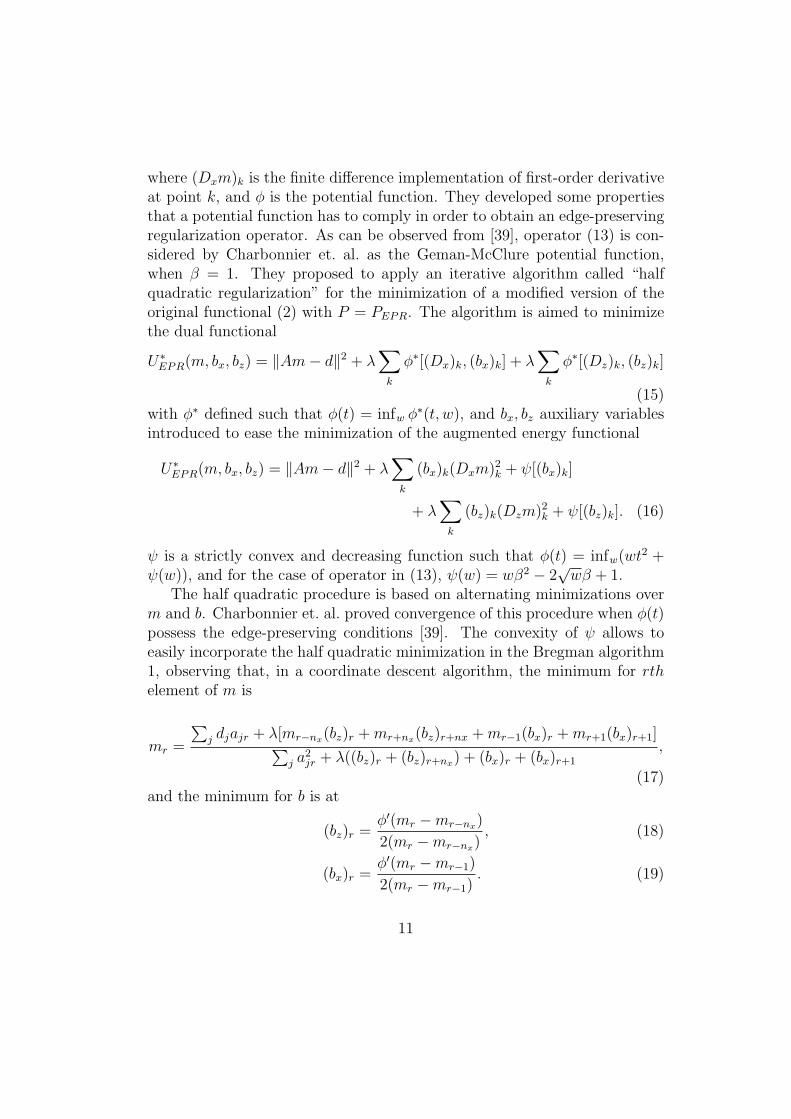
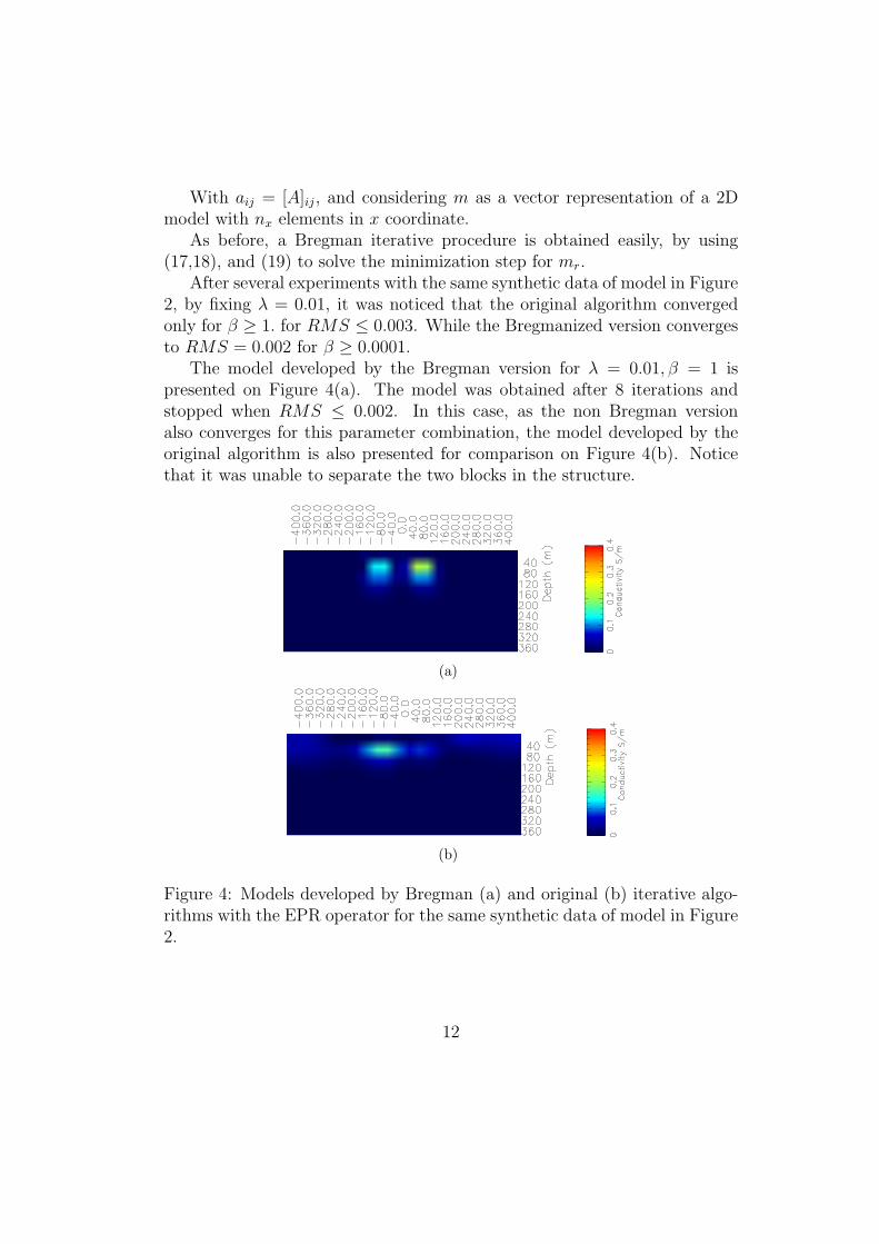
After several experiments with the same synthetic data of model in Figure2, by fixing λ = 0.01, it was noticed that the original algorithm convergedonly for β ≥ 1. for RMS ≤ 0.003. While the Bregmanized version convergesto RMS = 0.002 for β ≥ 0.0001.

The model developed by the Bregman version for λ = 0.01, β = 1 ispresented on Figure 4(a). The model was obtained after 8 iterations andstopped when RMS ≤ 0.002. In this case, as the non Bregman versionalso converges for this parameter combination, the model developed by theoriginal algorithm is also presented for comparison on Figure 4(b). Noticethat it was unable to separate the two blocks in the structure.

(a)

(b)

Figure 4: Models developed by Bregman (a) and original (b) iterative algo-rithms with the EPR operator for the same synthetic data of model in Figure2.

12

3.3 Hybrid operator

Now, consider the coordinate gradient descent algorithm presented for the1D case in [19]. There, an easily implementable iterative algorithm that doesnot require any optimization package was presented. In that algorithm, thecontinuation procedure that modifies the regularization operator has to becarefully tuned.

Here, we consider a Bregman iterative algorithm with the same hybridregularization operator, but not requiring a continuation procedure, provid-ing for more contrasted models. The proposed algorithm is based on Bregmaniteration with equations (6,7) and the hybrid regularization operator

PHybrid(m) = λ

(

α∑

i

|mi −mi∈Ni|+ 1− α

2

∑

i

(mi −mi∈Ni)2

)

(20)

with 0 ≤ α ≤ 1 a mixing parameter allowing to control the convex combina-tion of l1, l2 operators, and defining Nr = {mr−1,mr+1,mr−nx ,mr+nx} as thefirst order neighborhood ofmr. The minimization step of J(m)+ 1

2‖Am−dk‖22

is realized by a coordinate gradient-descent algorithm that solves for everyelement of m at a time, mk

r = T (mr), with T (·) the projection of m in[min,max]. mr is obtained as in [19]:

mk+1r =

1n

∑

i diair + λs1n

∑

i a2ir + nλ(1− α) (21)

where

di = di −p∑

j 6=r

aijmk+1j +

p∑

j=1

aijmkj , (22)

s = (1− α)(∑

j

mj∈Nr)− α(∑

j

ϕ(mr −mj∈Nr)), (23)

n = |Nr|, i.e. the number of neighbors of mr, and ϕ(x) is the subdiffer-ential of |x|, given by

ϕ(x) =

{

sgn(x) if x 6= 0

Co{−1, 1}, if x = 0.(24)

Equation 21 may have several solutions, here, as in [19], the implementa-tion consider the heuristic of using best solution (providing greatest descent)

13

of the ones obtained when ϕ(x) = {−1, 0, 1}. It should be noticed that theoriginal CGD algorithm implemented a continuation procedure because oflack of convergence when a constant α is considered. In this Bregman ver-sion of the algorithm, convergence is guaranteed by convergence propertiesobserved before and presented in Osher et. al. [20] for J(·) a convex operator.

After several experiments, convergence to a RMS fitness error lower than0.002 was obtained for λ = 0.01, for any α ∈ [0, 1]. More compact modelsare obtained with α near 1.

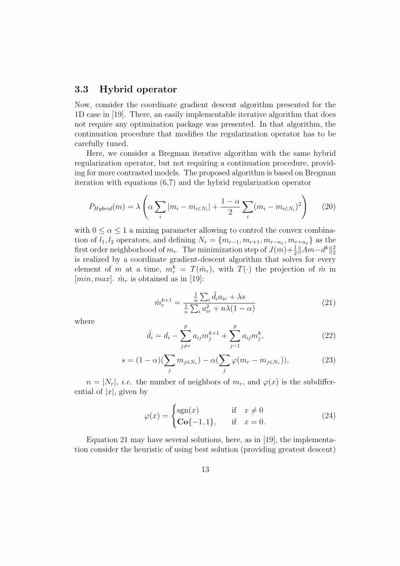
A model developed by applying this algorithm is presented on Figure 5for λ = 0.01, α = 0.2, and stopped when fitness to data was RMS ≤ 0.002,after 8 iterations.

It can be observed that the recovered model is free of staircase phe-nomenon, even for this low level of alpha, and possesses similar contrastas the original model.

Figure 5: Model developed by Bregman iterative algorithm with the CGDoptimization in the inner step for the same synthetic data of model in Figure2.

3.4 Numerical modeling comparison

The three original algorithms implement different alternatives to TV oper-ator. From them, only CGD is convex. EPR is solved by using the convexduality proposed by Charbonnier et. al. [39] and MGS is implemented withthe quadratic approximation used by Portniaguine and Zhdanov in [5]. Thosemodifications allow Bregman iterations to converge.

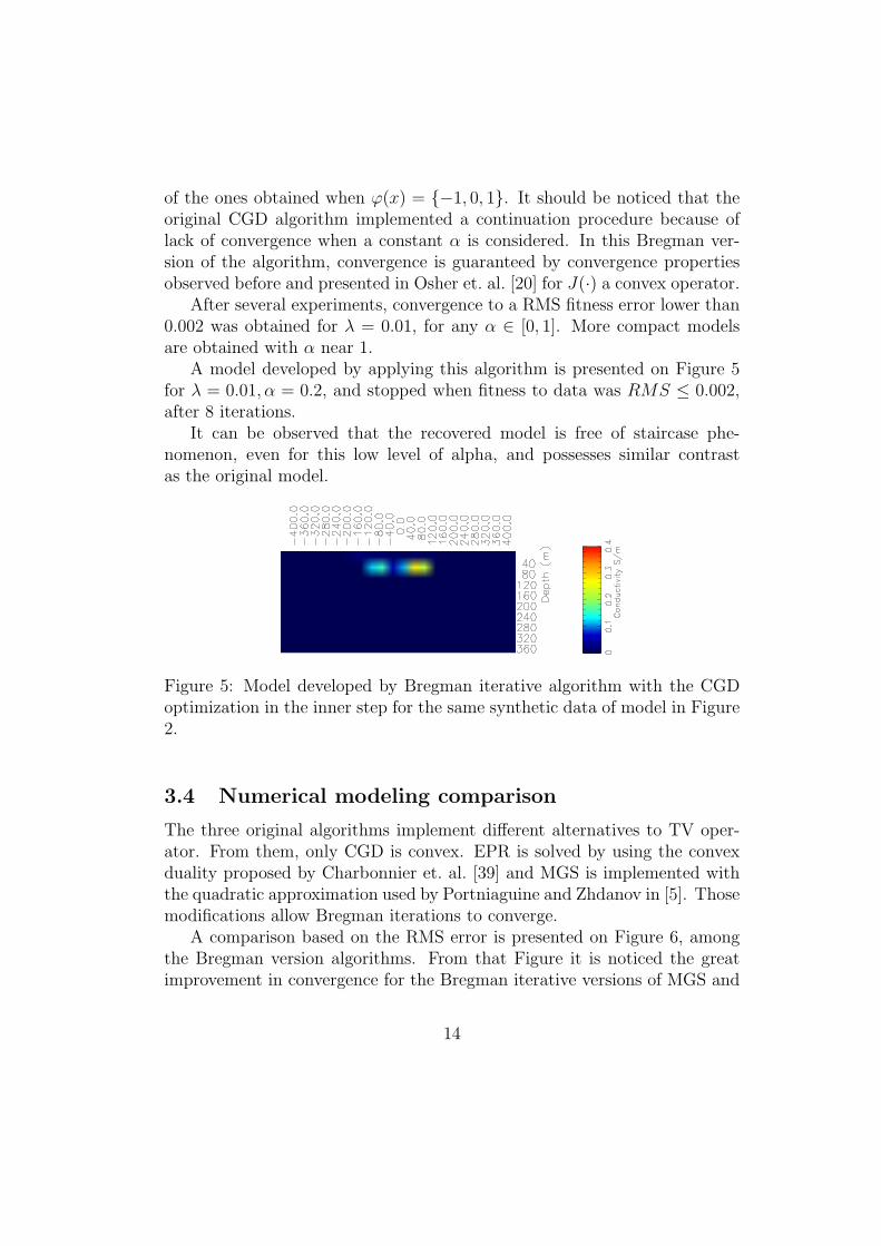
A comparison based on the RMS error is presented on Figure 6, amongthe Bregman version algorithms. From that Figure it is noticed the greatimprovement in convergence for the Bregman iterative versions of MGS and

14

CGD. The non-Bregman version of those algorithms should have to use acontinuation procedure on λ to achieve the same RMS fitness level. MGSseems to present the slowest convergence rate, requiring of 12 iterations toattain a fitness RMS of 0.002, but, as shown later, every iteration takes thelowest CPU time of all the tests. As for EPR, the original version does nothave convergence problems for the considered parameters (λ = 0.02, β = 1),but provides a recovered model of inferior quality as observed from the com-parison of Figure 4. Increasing β in MGS allows for better convergencewithout the variations on RMS for the first iterations, but some staircasingeffects on the resulting model are obtained. A CPU time comparison for thethree algorithms is observed on Table 2. The algorithms were implementedon a Intel Core i5 CPU @ 2.54GHzx4. It can be observed from that Tablethat MGS consumes the lowest amount of CPU, while EPR and CGD re-quire about the same time to obtain the final models on Figures 4(a) and5. Both MGS and CGD deliver more compact models, but CGD has betterconvergence due to the convexity of PHybrid operator.

0

0.005

0.01

0.015

0.02

0.025

2 4 6 8 10 12

RM

S

iterations

CGDEPRMGS

Figure 6: RMS error in every iteration for the Bregman versions of EPR,CGD and MGS algorithms for the same synthetic data of model in Figure 2.

4 Applications To Field Data

In this section we present applications of the iterative algorithms to fielddata. The object of the measurements was the mapping of unconsolidated

15

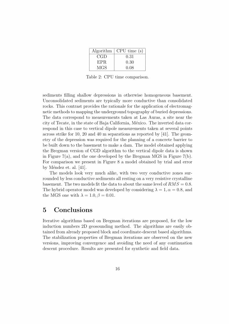
Algorithm CPU time (s)CGD 0.31EPR 0.30MGS 0.08

Table 2: CPU time comparison.

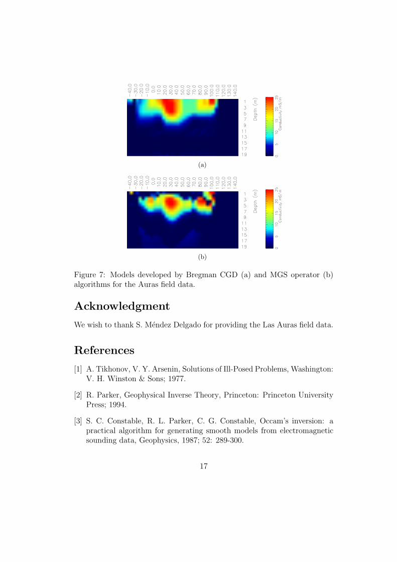
sediments filling shallow depressions in otherwise homogeneous basement.Unconsolidated sediments are typically more conductive than consolidatedrocks. This contrast provides the rationale for the application of electromag-netic methods to mapping the underground topography of buried depressions.The data correspond to measurements taken at Las Auras, a site near thecity of Tecate, in the state of Baja California, Mexico. The inverted data cor-respond in this case to vertical dipole measurements taken at several pointsacross strike for 10, 20 and 40 m separations as reported by [41]. The geom-etry of the depression was required for the planning of a concrete barrier tobe built down to the basement to make a dam. The model obtained applyingthe Bregman version of CGD algorithm to the vertical dipole data is shownin Figure 7(a), and the one developed by the Bregman MGS in Figure 7(b).For comparison we present in Figure 8 a model obtained by trial and errorby Mendez et. al. [41].

The models look very much alike, with two very conductive zones sur-rounded by less conductive sediments all resting on a very resistive crystallinebasement. The two models fit the data to about the same level ofRMS = 0.8.The hybrid operator model was developed by considering λ = 1, α = 0.8, andthe MGS one with λ = 1.0, β = 0.01.

5 Conclusions

Iterative algorithms based on Bregman iterations are proposed, for the lowinduction numbers 2D geosounding method. The algorithms are easily ob-tained from already proposed block and coordinate-descent based algorithms.The stabilization properties of Bregman iterations are observed on the newversions, improving convergence and avoiding the need of any continuationdescent procedure. Results are presented for synthetic and field data.

16

(a)

(b)

Figure 7: Models developed by Bregman CGD (a) and MGS operator (b)algorithms for the Auras field data.

Acknowledgment

We wish to thank S. Mendez Delgado for providing the Las Auras field data.

References

[1] A. Tikhonov, V. Y. Arsenin, Solutions of Ill-Posed Problems, Washington:V. H. Winston & Sons; 1977.

[2] R. Parker, Geophysical Inverse Theory, Princeton: Princeton UniversityPress; 1994.

[3] S. C. Constable, R. L. Parker, C. G. Constable, Occam’s inversion: apractical algorithm for generating smooth models from electromagneticsounding data, Geophysics, 1987; 52: 289-300.

17

Figure 8: Model developed by Mendez et. al. [41] by trial and error for theAuras field data.

[4] J. T. Smith and J. R. Booker, Rapid inversion of two- and three- dimen-sional magnetotelluric data, J. Geophys. Res., 1991; 96: 3905-3922.

[5] O. Portniaguine and M. S. Zhdanov, Focusing geophysical inversion im-ages, Geophysics, 1999; 64: 874-887.

[6] H. Hidalgo, J. L. Marroquın, E. Gomez-Trevino, Piecewise smooth modelsfor electromagnetic inverse problems, IEEE Transactions on Geoscienceand Remote Sensing, 1998; 36: 556-561.

[7] Iv. M. Varentsov, A general approach to the magnetotelluric data inver-sion in a piecewise-continuos medium. Izvestya, Phys. Solid Earth, 2002;38: 913-934.

[8] Iv. M. Varentsov, A general approach to the magnetotelluric data inver-sion in a piecewise-continuos medium. Izvestya, Phys. Solid Earth, 2002;38: 913-934.

[9] F. J. Esparza, E. Gomez-Trevino, Electromagnetic sounding in the resis-tive limit and the Backus-Gilbert method for estimating averages, Geo-exploration, 1987;24: 441-454.

[10] F. Esparza, E. Gomez-Trevino, 1-D inversion of resistivity and inducedpolarization data for the least number of layers, Geophysics, 1997; 62:1724-1729.

[11] H. Hidalgo, E. Gomez-Trevino, M. A. Perez-Flores, Linear programsfor the reconstruction of 2D images from Geophysical electromagnetic

18

measurements, Subsurface Sensing Technologies and Applications, 2004;5: 79-96.

[12] M. S. Zhdanov and E. Tolstaya, Minimum support nonlinearparametrization in the solution of a 3D magnetotelluric inverse problem,Inverse Problems, 2004; 20: 937-953.

[13] D. Dobson, Recovery of blocky images in electrical impedance tomogra-phy, in Engl, Louis, Rundell, editors, Inverse problems in medical imagingand nondestructive testing, New York: Springer; 1997, p. 43-64.

[14] C. Vogel, and M. Oman, Fast, robust total variation-based reconstruc-tion of noisy, blurred images, IEEE Transactions on Image Processing,1998; 7: 813-824.

[15] M. Benning, Singular Regularization of Inverse Problems. Ph.D. diss.,University of Muenster, Munster, 2011.

[16] C. R. Vogel, Computational methods for inverse problems, Philadelphia:SIAM; 2002.

[17] M. Z. Nashed, O. Scherzer, Least squares and bounded variation regular-ization with nondifferentiable functionals, Numerical Functional Analysisand Optimization, 1998;19: 873-901.

[18] T. Chan, S. Esedoglu, F. Park, A. Yip, Recent developments in totalvariation restoration in N. Paragio, O. Faugeras, editors, Handbook ofmathematical models in computer vision , New York: Springer; 2006, p.17-32.

[19] H. Hidalgo-Silva, E. Gomez-Trevino, Inversion of electromagneticgeosoundings using coordinate descent optimization, Inverse Problemsin Science and Engineering, DOI:10.1080/17415977.2012.743654

[20] S. Osher, M. Burger, D. Goldfarb, J. Xu, W. Yin, An iterated regular-ization method for total variation based image restoration, SIAM Journalon Multiscale Modeling and Simulation, 2005;4: 460-489.

[21] L. Rudin, S. Osher, E. Fatemi, Nonlinear total variation based noiseremoval algorithms Physica D, 1992; 60: 259-268.

19

[22] W. Yin, S. Osher, D. Goldfarb, J. Darbon, Bregman iterative algorithmsfor l1 minimization with applications to compressed sensing, SIAM Jour-nal of Imaging Science, 2008;1: 143-168.

[23] E. Esser, Applications of Lagrangian based alternating direction meth-ods and connections to split Bregman, UCLA: Computational AppliedMathematics CAM Report 09-31; 2009.

[24] M. R. Hestenes, Multiplier and gradient methods, Journal of Optimiza-tion Theory and Applications, 1969; 4: 303-320.

[25] M. J. D. Powell, A method for nonlinear constraints in minimizationproblems, in R. Fletcher, editor, Optimization, New York: AcademicPress; 1972, p. 283-298.

[26] W. Yin, S. Osher, Error forgetting of Bregman iteration, Journal ofScientific Computing, 2013; 54: 684-695.

[27] E. Haber, A mixed finite element method for the solution of the mag-netostatic problem with highly discontinuous coefficients in 3D, Compu-tational Geosciences, 2000;4: 323-336.

[28] Yan, G., Wang, J., Hao, Z., and Li, X., An extension of augmentedLagrange multiplier method for remote sensing inversion, in Geoscienceand Remote Sensing Symposium, Proceedings IGARSS’01; 2001 Jul 9;IEEE 2001 International; 2001.

[29] Delbos, F., Gilbert, J. Ch., Glowinski, R. and Sinoquet, D., Con-strained optimization in seismic reflection tomography: a GaussNew-ton augmented Lagrangian approach, Geophysical Journal International,2006; 164: 670-684.

[30] Wang, J., Ma, J., Han, B., Li, Q., Split Bregman iterative algorithm forsparse reconstruction of electrical impedance tomography, Signal Process-ing, 2012; 92: 2952-2961.

[31] Ma, J., Improved iterative curvelet thresholding for compressed sensing,IEEE Transactions on Instrumentation and Measurement, 2011; 60: 126-136.

20

[32] H. Hidalgo-Silva, and E. Gomez-Revino, Iterative Algorithms forGeosounding Inversion, Poster session presented at: 4th Inverse Prob-lems, Design and Optimization Symposium; 2013 June 27; Albi.

[33] F. S. Grant, G. G. West, Interpretation Theory in Applied Geophysics,New York: McGraw-Hill Book Company; 1965.

[34] J. D. McNeill: 1980, Electromagnetic terrain conductivity measurementsat low induction numbers, Technical Note TN-6, Geonics Ltd., Missis-sauga, Ontario, 1980.

[35] E. Gomez-Trevino,F. Esparza, S. Mendez-Delgado, ‘New theoreticaland practical aspects of electromagnetic soundings at low induction num-bers’, Geophysics, 2002; 67: 1441-1451.

[36] E. Gomez-Trevino: 1987, Nonlinear integral equations for electromag-netic inverse problems, Geophysics, 1987; 52: 1297-1302.

[37] M. A. Perez-Flores,S. Mendez-Delgado, E. Gomez-Trevino, Imaginglow-frequency and dc electromagnetic fields using a simple linear approx-imation, Geophysics, 2001; 66: 1067-1081.

[38] YH Dai, R. Fletcher, Projected Barzilai-Borwein methods for large-scalebox-constrained quadratic programming, Numerische Mathematik, 2005;100: 21-47.

[39] P.Charbonnier, L. Blanc-Feraud, G. Aubert, M. Barlaud, Determinis-tic edge-preserving regularization in computed imaging, IEEE Tran. onImage Processing, 1997; 6: 298-311.

[40] H. Hidalgo-Silva, E. Gomez-Trevino, J. L. Marroquın and F.J. Esparza,Piecewise continuous models for resistivity soundings, IEEE Tran. Geo-science and Remote Sensing, 2001, 39; 2725-2728.

[41] S. Mendez Delgado, E. Gomez-Trevino, and M. A. Perez-Flores, Forwardmodelling of direct current and low-frequency electromagnetic fields usingintegral equations, Geophys. J. Int. 1999; 137: 336-352.

21