arX

iv:2

111.

0276

4v1

[m

ath.

NA

] 4

Nov

202

1

Stabilization and Variations to the Adaptive Local Iterative

Filtering Algorithm: the Fast Resampled Iterative Filtering Method

Giovanni Barbarino∗, Antonio Cicone†

November 5, 2021

Abstract

Non-stationary signals are ubiquitous in real life. Many techniques have been proposed in the last

decades which allow decomposing multi-component signals into simple oscillatory mono-components,

like the groundbreaking Empirical Mode Decomposition technique and the Iterative Filtering method.

When a signal contains mono-components that have rapid varying instantaneous frequencies, we can

think, for instance, to chirps or whistles, it becomes particularly hard for most techniques to properly

factor out these components. The Adaptive Local Iterative Filtering technique has recently gained

interest in many applied fields of research for being able to deal with non-stationary signals presenting

amplitude and frequency modulation. In this work, we address the open question of how to guarantee

a priori convergence of this technique, and propose two new algorithms. The first method, called Stable

Adaptive Local Iterative Filtering, is a stabilized version of the Adaptive Local Iterative Filtering that

we prove to be always convergent. The stability, however, comes at the cost of a higher complexity in the

calculations. The second technique, called Resampled Iterative Filtering, is a new generalization of the

Iterative Filtering method. We prove that Resampled Iterative Filtering is guaranteed to converge a priori

for any kind of signal. Furthermore, in the discrete setting, by leveraging on the mathematical properties

of the matrices involved, we show that its calculations can be accelerated drastically. Finally, we present

some artificial and real-life examples to show the powerfulness and performance of the proposed methods.

1 Introduction

The analysis and decomposition of non-stationary signals is an active research direction in both Mathematicsand Signal Processing. In the last decades many new techniques have been proposed. Among them, theIterative Filtering (IF) algorithm [20] was proposed a decade ago as an alternative technique to the celebratedEmpirical Mode Decomposition (EMD) technique [17] and its variants [28, 30, 25, 31]. The EMD and itsvariants, in fact, were missing a rigorous mathematical analysis, due to the usage of a number of heuristicand ad hoc elements. Some results have been presented in the literature [15, 26, 16], but a complete rigorousmathematical analysis is still missing nowadays.

The EMD-like methods are based on the iterative computation of the signal moving average via envelopesconnecting its extrema. The computation of the signal moving average allows to split the signal itself into asmall number of simple oscillatory components, called Intrinsic Mode Functions (IMFs), which are separatedin frequencies and almost uncorrelated [11]. The IF method has been developed following the same structureof EMD, but with a key difference: the moving average is now obtained through an iterated convolutionalfiltering operation on the signal, with the aim to single out all its non-stationary components, starting fromthe highest frequency one.

The IF algorithm structure allowed to develop a complete mathematical analysis of this method [8, 12, 14].On the other side, this method is “rigid” in the sense that it allows to extract only IMFs which are amplitudes

∗Department of Mathematics and Systems Analysis, Aalto University, Finland. giovanni.barbarino@aalto.fi†DISIM, Universita degli Studi dell’Aquila, L’Aquila, Italy, and Istituto di Astrofisica e Planetologia Spaziali, INAF, Roma,

Italy, and Istituto Nazionale di Geofisica e Vulcanologia, Roma, Italy. antonio.cicone@univaq.it

1

modulated, but almost stationary in frequencies. This is a clear limitation if the signal contains chirps orwhistles, that are components with quickly changing instantaneous frequencies. For this reason in [12] theauthors proposed a generalization of IF called Adaptive Local IF (ALIF). ALIF does not suffer anymore ofthe rigidity of IF in extracting IMFs containing rapidly varying instantaneous frequencies. However, thisnew technique loses most of mathematical background of IF. Even if the algorithm gained visibility sinceits introduction five years ago, we can mention here, for instance, [1, 2, 3, 4, 5, 18, 19, 21, 22, 23, 29], aninitial mathematical analysis has been only recently developed [10, 13], and much more study on extensions,variations and stabilization methods is currently ongoing, see, for instance, [6].

Due to the missing theoretical background of the ALIF method, in this paper we introduce two newalgorithms for which such analysis is possible. The first, called Stable ALIF (SALIF) method, is alwaysconvergent, even in presence of noise, but it presents an increased computational cost with respect to ALIF.The second, called Resampled IF method (RIF), is actually a modification of the IF algorithm, that preservesIF convergence property, but, at the same time, presents the same flexibility as ALIF. Furthermore RIFmethod can be made, in the discrete case, highly computational efficient via the FFT computation of theconvolutions, in what is called the Fast Resampled IF method (FRIF).

The rest of this paper is structured as follows. Section 2 is a review of the IF and ALIF methods, andintroduces the new SALIF method. Here we compare their features, stressing their strength and weaknesses.Section 3 is dedicated to the RIF algorithm, its analysis, properties and acceleration via FFT, in what iscalled FRIF technique. In this section we show how RIF combines the convergence and stability of IF withthe flexibility of ALIF, and how it can be made computationally efficient. In Section 4 we compare thosealgorithms on artificial and real data, reporting the efficiency and accuracy of each method. Eventually, inSection 5, we draw conclusions and suggest future lines of research.

2 Iterative Filtering based Methods

Throughout this document, a signal is intended to be a real function g : R → R, and we study its behaviourin the reference interval [0, 1]. Outside this interval the signal is usually not known, and so we have toimpose some boundary conditions, discussed for example in [9] and [24]. In particular, in [24], the authorsshow how any signal can be pre-extended and made periodical at the boundaries. Therefore, from now on,for simplicity and without losing generality, we will assume that the signals to be decomposed are alwaysperiodical at the boundaries.

The Iterative Filtering (IF) methods mimics the EMD algorithm in the application of a moving averagethat captures the main trend of the signal, and allows us to decompose it into simple IMF components. Ifwe call L(g) the moving average, then both EMD and IF algorithms extract the first IMF as

S(g) = g − L(g), IMF1 = limm→∞

Sm(g). (1)

Repeating iteratively the same procedure on r = g − IMF1, we can extract all the IMFs until r becomes atrend signal, meaning that it possesses at most two extrema.

The difference between these two algorithms is that, while for EMD the moving average operator L(g) ischanging at each iteration and depends completely on the shape of a given signal, in IF L(g) can be rewrittenas the convolution of g with what is called a filter k. Here a filter k is an even, nonnegative, bounded andmeasurable real function with compact support and unit mass, meaning

∫Rk(z) dz = 1.

A generalization of the IF method is called Adaptive Local Iterative Filtering (ALIF), and utilizes theconvolution with a family of filters kx(z) as moving average, whose support is in [−ℓ(x), ℓ(x)], i.e. it varieswith x. Therefore, the moving average computation operator can be written as

L(g)(x) =

∫ 1

0

g(z)kx(x − z) dz, (2)

2

Following [12], we can rewrite the same expression as

L(g)(x) =

∫ L

−L

g(x+ t(x, z))k(z) dz, (3)

where k(z) is a filter with constant support in [−L,L] and t(x, z) is a measurable function. In the followingsubsections we report the most common choice for the filters, and a description of the resulting method.

2.1 Linear ALIF

When we talk about the ALIF method, we usually refer to Linear ALIF. After having fixed a filter k(z) withsupport [−1, 1], and a positive “length” function ℓ(x), then the linear ALIF method prescribes

kx(z) := k

(z

ℓ(x)

)1

ℓ(x)in (2), or equivalently t(x, z) = −ℓ(x)z in (3).

Notice that kx(z) is a filter with support [−ℓ(x), ℓ(x)] for every x ∈ [0, 1].Given now a signal g(z), we can compute a length function ℓ(x), that usually depends on the relative

positions of local extrema in g(z) if the signal does not contain noise, and apply the iteration in (1) with theappropriate filter.

S(g)(x) = g(x)−

∫ 1

0

g(z)k

(x− z

ℓ(x)

)dz

ℓ(x), IMF1 = lim

m→∞

Sm(g). (4)

Repeating iteratively the same procedure on r = g − IMF1, we obtain a decomposition of the signal g intoIMFs. Notice that ℓ(x) changes after we identify each different IMFs. Here we report the resulting algorithm.

Algorithm 1 (ALIF Algorithm) IMFs = ALIF(g)

IMFs = {}initialize the remaining signal r = gwhile the number of extrema of r is ≥ 2 dofor each x ∈ [0, 1] compute the length function ℓ(x), depending on rg1 = rm = 1while the stopping criterion is not satisfied do

gm+1 = gm −∫ 1

0 gm(z)k(

x−zℓ(x)

)dzℓ(x)

m = m+ 1end whileIMFs = IMFs ∪ {gm}r = r − gm

end while

The operation S(g) = g−L(g) is designed to catch the fluctuation part of the signal, that usually presentshigh frequency. The operation is iterated until a stopping criterion is satisfied, usually regarding the norm ofthe difference gm+1− gm, or the number of iterations themselves. For more details on the stopping criterion,we refer the interested reader to [12, 20]. The IMFs are thus extracted from the signal until it becomes justa trend signal with 2 or less extrema. Since the sum of all the IMFs and the trend signal returns the originalsignal, it can effectively be called a decomposition.

Regarding the length function ℓ(x) identification in signals containing noise, we observe that it is alwayspossible to first run a time-frequency representation (TFR) algorithm, see [27] for a comprehensive review ofmodern TFR techniques, and then use the acquired information to designed the optimal ℓ(x). This procedureis really important for ALIF algorithm, but it is also a research topic per se. This is why, from now on, we

3

assume that the length function can be computed accurately and we postpone the analysis of how actuallycompute it to a future work.

Conceptually, the ALIF method separates non-stationary components of the signal, even with varyingamplitudes, starting from the highest frequencies. For example, on real data, the method first extract highfrequency noise IMFs, and then starts to produce clean components. The main feature of the produced IMFsis that their instantaneous frequencies are pointwise sorted in decreasing order. In formulae, if Fk(x) is theinstantaneous frequency of the k-th IMF at the point x ∈ (0, 1), we have that

F1(x) > F2(x) > F3(x) > . . . ∀x ∈ (0, 1).

The method, albeit being very powerful and having already been utilized in a variety of applications, stilllacks a theoretical analysis proving the convergence of (4), except in a few notorious cases [6, 10, 12]. In thenext sections, we report some of the available convergence results for the discrete version of the algorithm.

2.2 Discrete ALIF and Stabilization

Usually in a discrete setting, a signal is given as a vector of sampled values g = [g0 g1 . . . gn−1] wheregi = g(xi) and xi = i/n for i ∈ Z. As a consequence, one can discretize the relation (2) with a simplequadrature formula.

L(g)(xi) =

∫ 1

0

g(z)kxi(xi − z) dz ≈

1

n

n−1∑

j=0

gjkxi(xi − xj)

In turn, this lets us write the sampling vector of S(g), called g, as a matrix-vector multiplication. In fact, ifwe assume all the indexes start from zero,

S(g)(xi) = gi − L(g)(xi) =⇒ g = (I −K)g, Ki,j =

[1

nkxi

(xi − xj)

]n−1

i,j=0

.

In the Linear ALIF paradigm, we fix a filter k(z) and choose a length function ℓ(x) depending on the signal,to produce our family of filters kx(z) = k(z/ℓ(x))/ℓ(x). The resulting algorithm is reported here.

Algorithm 2 (Discrete ALIF Algorithm) IMFs = ALIF(g)

IMFs = {}initialize the remaining signal r = g

while the number of extrema of r is ≥ 2 docompute ℓ(x) and the matrix Kg1 = r

m = 1while the stopping criterion is not satisfied dogm+1 = (I −K)gmm = m+ 1

end whileIMFs = IMFs ∪ {gm}r = r − gm

end while

From the algorithm, it is evident that the convergence of the internal loop only depends on the spectralproperties of the matrix I −K. In fact, since gm+1 = (I −K)mg1, we find that a necessary condition forthe convergence is

|1− λi(K)| ≤ 1, ∀i = 1, . . . , n. (5)

If the zero eigenvalue of K has equal geometric and algebraic multiplicities, and it is the only eigenvalue forwhich |1− λi(K)| = 1, then the condition is also sufficient. From the same analysis, one can notice that the

4

algorithm actually produces a projection of the signal g on the approximated null space of K.

Notice that if A is an invertible matrix, then Null(AK) = Null(K), meaning that substituting AK inthe algorithm doesn’t significantly change the output. As a consequence, we can always suppose that K is astochastic matrix, so that we don’t have to worry about large λi(K). Nonetheless, we still cannot assert theabsence of negative or complex eigenvalues which are not fulfilling the relation (5). Recent studies [10, 6]show that for large n and continuous functions k(z), ℓ(x), almost all eigenvalues of the matrix K are realand nonnegative, but it is still not enough to establish the convergence of the method. Moreover, it has beenascertained experimentally that such cases may arise, especially whit a fast changing function ℓ(x).

A simple way to stabilize the method is to choose A = ‖K‖−2KT , so that AK is a nonnegative matrixthat is also positive semidefinite, with all the eigenvalues bounded by 1. Notice that we can also use c−2

instead of ‖K‖−2, where c = maxj∑

iKi,j , or in general any constant satisfying ‖cK‖ ≤ 1. We call theresulting method Stable ALIF (SALIF).

Algorithm 3 (Stable Discrete ALIF Algorithm) IMFs = SALIF(g)

IMFs = {}initialize the remaining signal r = g

while the number of extrema of r is ≥ 2 docompute ℓ(x) and the matrix Kg1 = r

m = 1while the stopping criterion is not satisfied dogm+1 = (I −KTK)gmm = m+ 1

end whileIMFs = IMFs ∪ {gm}r = r − gm

end while

The method is called stable since a perturbation of the matrix K does not prevent the convergence ofthe inner loop. Moreover, we will show in the experiments, ref. Section 4, that SALIF is able to producemore accurate solutions than the other methods.

The algorithm, though, comes with an increased computational cost with respect to ALIF, mainly dueto two factors.

• The iterative step in the SALIF algorithm gm+1 = (I −KTK)gm takes at least double the time withrespect to the respective step in the ALIF algorithm. Since the number of iterations is usually muchsmaller than n, even computing KTK beforehand does not improve the speed.

• The order of the smallest eigenvalues of KTK is approximately the square of the smallest ones inK. The algorithm thus requires more iterations to attain the same accuracy of ALIF, since it mustseparate eigenspaces that are now closer.

A different way to stabilize the method is to take ℓ(x) constant, producing a much faster algorithm, i.e. theIF algorithm, whose spectrum of application is though more limited.

2.3 IF and Discrete IF

When we talk about the IF method, we refer to the linear ALIF method with constant length functionℓ(x) = L in (4), or equivalently, where t(x, z) = −Lz in (3). The IF method only separates IMF componentsof the signal which are amplitude modulated, but quasi-stationary in frequency, starting from the highestfrequencies. Nevertheless, it has been proved [15] that in this case the iterations (4) always converge whenever

5

k(z) is a filter with nonnegative Fourier transform. The condition is satisfied, for example, by k = ω ⋆ ω,where ω is a generic filter and ⋆ is the convolution operator.

In the discrete setting, the IF algorithm has the advantage of a fast implementation based on FFT, inwhat is called Fast Iterative Filtering (FIF), and an advanced theoretical analysis [8, 14]. Recall that we onlyknow the signal g(x) on the interval [0, 1], so we can always suppose that the original signal is 1-periodic (forexample, by reflecting the signal on both sides and making it decay [24]). We can thus rewrite the movingaverage (2) as

L(g)(x) =

∫

R

g(z)k

(x− z

L

)dz

L, S(g) = g − L(g) (6)

and discretize it on a regular grid xi = i/n of [0, 1]. Here, the integral is always well-defined, since the filterhas compact support. Moreover L is inversely proportional to the target frequency of the extracted IMF,and L ≥ 1/2 usually indicates that we already have a trend signal g, so we always suppose 1/L > 2.

Following the same steps as in the ALIF algorithm, we find

L(g)(xi) ≈1

nL

∑

j∈Z

gjk(xi−j

L

)

Notice that the above formula can be expressed through a Hermitian circulant matrix K with first row

1

nM

[k(0), k

(1

nL

), . . . , k

( s

nL

), 0 . . . 0, k

( s

nL

), . . . , k

(1

nL

)]

where s = ⌊nL⌋ < ⌊n/2⌋. The sampling vector g of S(g) on the points x0, x1, . . . , xn−1, can be thus rewrittenas a matrix-vector multiplication

S(g)(xi) = gi − L(g)(xi) =⇒ g = (I −K)g. (7)

The resulting algorithm is thus the same as Algorithm 2, but where K is Hermitian and circulant. The IFmethod is consequently much faster than the ALIF algorithm since the multiplication (I − K)gm can beperformed very efficiently through an FFT. Actually, in [14] we can find an even faster implementation, theso called FIF algorithm, and the proof that K is also positive semidefinite.

Keeping in mind that, as in ALIF, we can always multiply K by a diagonal matrix and make it stochastic,we have the following result.

Lemma 1 ([14, Theorem 1, Corollary 3]) Given a double-convoluted filter k = ω ⋆ ω, then for the IFoperator S(·) in (6) the limit

limm→∞

Sm(g)

converges for any function g(x). Moreover, if L ≤ 1/2, then for the IF matrix K in (7) the limit

limm→∞

(I −K)mg

converges for any vector g.

To summarize, we have

• the IF and FIF algorithms always converge and are very fast, but cannot capture non-stationarycomponents with quickly varying frequencies,

• the ALIF algorithm is enough flexible to extract fully non-stationary components, but its convergenceis not guaranteed,

• the SALIF algorithm is always convergent and it has an output which is more accurate than the ALIFalgorithm one, but it is very slow.

In the next section, we show how to design an alternative method, that is flexible enough to perform non-stationary analysis on the signals, but at the same time fast and provably convergent.

6

3 Resampled Iterative Filtering

The linear ALIF method makes use of a length function ℓ(x) to locally stretch a fixed filter k(z) so that theconvolution with the signal g(z) smooths out the high oscillatory behaviour. The idea behind the ResampledIterative Filtering (RIF) algorithm is to set a fixed length for k(z) and instead modify the signal througha global resampling function. In a sense, we want to locally stretch the signal, making the component ofhigher frequency approximately stationary, so that we are able to identify it through the fast IF algorithm.

Given a resampling function G : [0,M ] → [0, 1] that is increasing and regular enough, the moving averagefor the RIF method will coincide with the IF one applied on g ◦G, as

L(g ◦G)(y) =

∫

R

g(G(z))k(y − z) dz,

where we assume that the resampled signal is M -periodic. If we consider the first-order expansion of G(x),and after a change of variable x = G(y), r = zG′(y), we have

∫

R

g(G(z)) k(y − z) dz =

∫

R

g(G(y − z)) k(z) dz

≈

∫

R

g(G(y)− zG′(y)) k(z) dz

=

∫

R

g(x− r) k

(r

G′(G−1(x))

)dr

G′(G−1(x))

=

∫

R

g(r) k

(x− r

G′(G−1(x))

)dr

G′(G−1(x))(8)

that is analogous to the linear ALIF moving average in (4), where, equivalently,

ℓ(x) = G′(G−1(x)) or G−1(x) =

∫ x

0

1

ℓ(t)dt. (9)

With (9), now we have a way to derive the resampling function from the length ℓ(x). The full RIF algorithmis thus reported as Algorithm 4.

Algorithm 4 (Resampled IF Algorithm) IMFs = RIF(g)

IMFs = {}initialize the remaining signal r = gwhile the number of extrema of r is ≥ 2 docompute ℓ(x) and derive the resampling G(y), G−1(x) and the resampled signal h = r ◦Gh1 = hm = 1while the stopping criterion is not satisfied dohm+1 = hm −

∫Rhm(y)k(x− y)dy

m = m+ 1end whileIMFs = IMFs ∪ {hm ◦G−1}r = r − hm ◦G−1

end while

From the algorithm it is evident that, after the resampling, the steps are the same of the IF algorithm. Infact, we always extract almost stationary IMFs from the resampled signal, and then we operate the inversesampling to obtain the respective IMFs for the original signal. Moreover, we point out that G(x) dependson ℓ(x), so it must be computed every time we want to extract a new component.

7

This observation is also enough to show that the internal loop always converge to some IMF. In the nextsection we see how these properties carry to the discrete case.

Notice that RIF is actually a particular ALIF method, since∫

R

g(G(x− z)) k(z) dz =

∫

R

g(x+ [G(x − z)− x]) k(z) dz

with t(x, y) = G(x − z)− x in (3).From the relations (8), we can say that Linear ALIF is a first-order approximation of RIF, and since RIF

is a convergent method, we could ask whether it produces the same output as Linear ALIF. The answer isprovided in the following

Theorem 1 The RIF method produces the same output as the Linear ALIF algorithm only when ℓ(x) is aconstant function, i.e. when the linear ALIF algorithm reduces to IF.

The proof follows from the observation that the derivation of equation 8 holds true only if

G(y − z) = G(y)−G′(y)z, ∀y, z

meaning that G′(z) = ℓ(G(z)) is constant for every z.

3.1 Fast Resampled Iterative Filtering

First of all we review how to possibly implement a discrete version of RIF. One way is by discretizing theIF moving average on the resampled signal, as in

gm+1(G(x)) = gm(G(x)) −

∫

R

gm(G(y)) k(x − y)dy.

Notice that hm = gm ◦G has domain [0,M ], so we need to discretize it on the regular grid xi := Mi/n for

i = 0, . . . , n− 1. Recall that M =∫ 1

0 ℓ(x)−1 dx and that in the IF algorithm, a constant L ≥ 1/2 indicatesthat g(x) is already a trend signal. This shows that we can safely assume ℓ(x) < 1/2 and thus M > 2.

We now extend the signal cyclically on the real line, meaning that hm(sM + x) := hm(x) for every s ∈ Z

and every x ∈ [0,M). The quadrature rule on the discretization points yields

hm+1(xi) ≈ hm(xi)−M

n

∑

j∈Z

hm(xj)k(xi − xj).

Notice that the above formula coincides with the IF moving average with length L = 1/M , and can beexpressed through a Hermitian circulant matrix K with first row

k1 =M

n

[k(0), k

(M

n

), . . . , k

(sM

n

), 0 . . . 0, k

(sM

n

), . . . , k

(M

n

)]

where s = ⌊n/M⌋. The moving average thus becomes

hm+1 = (I −K)hm

where I − K is still a Hermitian and circulant matrix, so that the matrix vector multiplication can beperformed efficiently through a FFT. In particular,

hm+1 = iDFT ((1 −DFT(k1)) ◦DFT(hm)) ,

where ◦ stands for the Hadamard (or element-wise) product between vectors, and DFT, iDFT stand forDiscrete Fourier Transform and its inverse, respectively. Moreover, since

DFT(hm+1) = (1−DFT(k1)) ◦DFT(hm)

8

Algorithm 5 (Fast Resampled Iterative Filtering) IMFs = FRIF(g)

IMFs = {}initialize the remaining signal r = g

while the number of extrema of r is ≥ 2 docompute ℓ(x), the resampling functions G−1(x) =

∫ℓ(t)−1 dt, the constant M = G−1(1) and the matrix

Kcompute the vector h through interpolation of r on the points G(yi) where yi = Mi/nh1 = h

h1 = DFT(h1), k1 = 1−DFT(k1)m = 1while the stopping criterion is not satisfied dohm+1 = k1 ◦ hm

m = m+ 1end whilehm = iDFT(hm)compute the vector I through interpolation of hm on the points G−1(yi) where yi = i/nIMFs = IMFs ∪ {I}r = r − I

end while

and since the stopping criterion can be checked on DFT(hm), we can further accelerate the method bycomputing the DFTs on h1 and k1 and the iDFT outside the loop, thus avoiding iterated computations ofFourier transforms.

The resulting method is reported in Algorithm 5.Notice that while the internal loop only consists of Hadamard multiplications among vectors, and its

convergence properties can be analysed with the same tools used for the IF algorithm [8, 14], in the outerloop we perform operations that may lead to a loss in accuracy of the method. We can thus adopt a splineinterpolation to mitigate the accuracy loss, and even in this case, the computational cost of the outer loopis still O(n log n) operations due to the Fourier transforms.

As for the previous algorithms the matrix K, and thus the vector k1, can be multiplied by a constant toupper bound its eigenvalues, and from Lemma 1 one can state an analogous convergence result.

Corollary 1 Given a double-convoluted filter k = ω⋆ω, then the inner loop of the RIF Algorithm 4 convergesfor any initial function h(x). Moreover, if M > 2, then in the FRIF Algorithm 5 the limit

limm→∞

hm = limm→∞

km1 ◦ h1

converges for any vector h1.

We have seen that the FRIF algorithm is provably convergent, and that its computational time is com-parable with the FIF method. In the numerical examples, we will also show that empirically it producessensible decompositions, but first let us address another property of the method.

3.2 Anti-Aliasing Property

In the discrete setting, the resampling of the signal g(x) may in theory come with an undersampling of thehighest frequencies, leading to aliasing effects. Here we show that in the FRIF algorithm, this is actuallynot a problem.

Suppose that the signal can be split into components I1(x), I2(x), . . . , where I1(x) has the highest in-stantaneous frequency among all the components. In the FRIF algorithm we choose the resampling G(x)

where G−1(z) =∫ x

0 ℓ(t)−1 dt and M = G−1(1) =∫ 1

0 ℓ(t)−1 dt. The resampled signal h(x) = g(G(x)) has

9

thus domain [0,M ], but in the discrete setting we treat it as a signal over [0, 1], so we are actually workingwith

h(x) = h(Mx) = g(G(Mx)).

The signal h(x) presents now a new decomposition in components J1(x), J2(x), . . . , where Ji(x) = Ii(G(Mx))and if ai(x) was the instantaneous frequency of Ii(x), then the respective frequency of Ji(x) is ai(G(Mx))G′(Mx)M .Notice that the function G(z) is chosen so that J1(x) is now approximately a stationary signal, so

β ≈ a1(G(Mx))G′(Mx)M = a1(G(Mx))ℓ(G(Mx))M,

for some constant β and for every x ∈ [0, 1]. As a consequence,

a1(G(Mx))G′(Mx)M =

∫ 1

0

a1(G(Mx))G′(Mx)

ℓ(t)dt ≈

∫ 1

0

a1(t) dt

that is surely less than ‖a1(x)‖∞. Moreover, since G(z) is increasing and a1(x) ≥ ai(x)∀x, i, then

a1(G(Mx))G′(Mx)M ≥ ai(G(Mx))G′(Mx)M, ∀x

meaning that J1(x) has still the biggest instantaneous frequency among the Ji(x). This proves that theresampling does not create artificial high frequency components, so the FRIF algorithm does not suffer fromaliasing problems.

3.3 Avoiding Interpolation

As pointed out before, the interpolations may introduce a loss in accuracy on the output of Algorithm5. One can though formulate a different, but equivalent, version of the continuous algorithm that doesnot require a resampling of the signal. Taking from the start of (8), let H(x) := G−1(x), x := G(y) andr := G(y)−G(y − z), so that z = y −G−1(G(y)− r) = H(x)−H(x− r).

∫

R

g(G(z)) k(y − z)dz =

∫

R

g(G(y − z)) k(z)dz

=

∫

R

g(x− r) k(H(x) −H(x− r))H ′(x− r)dr

=

∫

R

g(r) k(H(x) −H(r))H ′(r)dr.

As a consequence, we can discretize the relation

gm+1(x) = gm(x) −

∫

R

gm(r) k(H(x) −H(r))H ′(r)dr

by applying a quadrature rule on the points xi = i/(n− 1), as

gm+1(xi) ≈ gm(xi)−1

n− 1

∑

j∈Z

gm(xj)k(H(xi)−H(xj))H′(xj)

that coincides with multiplying the discretized signal gm by the matrix In −AnDn, where

An =

[k(H(xi)−H(xj))

n− 1

]n−1

i,j=0

=

k(H

(i

n−1

)−H

(j

n−1

))

n− 1

n−1

i,j=0

, Dn = diag(H ′(xi)

n−1i=0

).

Notice that Dn is positive definite, since from (9), H ′(x) = ℓ(x)−1 > 0 and An is symmetric since the filterk is an even function. If we call BN the matrix AN in the case H(x) ≡ x, then by Corollary 3 of [14],

10

BN is positive semidefinite. Since for a big enough N , the matrix An is approximated up to an arbitrarysmall error by a n× n principal submatrix of the matrix BN , then we can conclude that An is also positivesemidefinite. As a consequence,

In −AnDn ∼ In −D1/2n AnD

1/2n

and all its eigenvalues are real and less than 1. Eventually, as in the precedent algorithms, the matrixAnDn can be multiplied by a constant so that its eigenvalues are upper bounded for example by 1, so thatΛ(In −AnDn) ⊆ (−1, 1] and the method becomes provably convergent.

The resulting algorithm is thus equivalent in its continuous version to Algorithm 4, and in its discreteversion it avoids the need to interpolate the signal two times per IMF. Moreover, its internal loop has beenproved to be convergent and it presents the same flexibility properties as ALIF.

At the same time, though, the matrix AnDn is not cyclic, so we lose the fast implementation that waspossible in Algorithm 5. For this reason, we do not test this version of the RIF algorithms in the followingnumerical experiments.

4 Numerical Experiments

In this section we show and compare the performances of all the reviewed techniques. In order to studythe signals and their decompositions in time-frequency, we will rely on the so called IMFogram, a recentlydeveloped algorithm [7], which allows to represent the frequency content of all IMFs. The IMFogram provesto be a robust, fast and reliable way to obtain the time-frequency representation of a signal, and it has beenshown to converge, in the limit, to the well know spectrogram based on the FFT [11].

The following tests have been conducted using MATLAB R2021a installed on a 64–bit Windows 10 Procomputer equipped with a 11th Gen Intel Core i7-1165G7 at 2.80GHz processor and 8GB RAM. All testedexamples and algorithms are freely available at 1.

4.1 Example 1

We consider the artificial signal f , plotted in the left panel, bottom row, of Figure 1, which contains twononstationary components with exponentially changing frequencies f1 and f2, plus a trend f3. In particular

f1(x) = cos(20etπ + 120πt)

f2(x) = cos(20etπ + 20πt)

f3(x) = −10x+ 20

where x vary in [0, 1] and is sampled over 104 points.The f1 and f2 components and f signal are plotted in the left panel of Figure 1, whereas f1 and f2

frequencies are shown in the central panel.in Table 1 we report the computational time required by ALIF, SALIF and FRIF with a fixed stopping

criterion. In the same table we summarize the performance of the three techniques in terms of inner loopiterations required to produce the two IMFs and the relative error measured as ratio between the norm 2of the difference between the computed IMF and the corresponding ground truth, and the norm 2 of theground truth itself.

From Table 1 results it is clear that FRIF proves to converge quickly to a really accurate solution.In fact, it takes less than a second to produce a decomposition which has a relative error which is orderof magnitudes smaller than the ones produced using ALIF and SALIF methods. Furthermore ALIF andSALIF decompositions require more than 16 and 26 seconds, respectively, to converge. This is confirmed bythe results shown in the right panel of Figure 1, where we compare the norm 2 relative error of the IMF1

1www.cicone.com

11

-0.5

0

0.5

-0.5

0

0.5

14

16

0.3 0.35 0.4 0.45 0.5 0.55 0.6 0.65 0.7 0.75

12

14

16

18

0.3 0.35 0.4 0.45 0.5 0.55 0.6 0.65 0.7 0.75

300

400

500

600

700

800

900

1000

100 200 300 400 500

10 -2

10 0

Figure 1: Example 1. Left panel: the components f1 and f2, respectively first and second row,the trend,third row, and the signal f , bottom row. Central panel: exponential instantaneous frequencies of f1 and f2.Right panel: relative error in norm 2 between the ground truth and IMF1 produced by ALIF, SALIF, andFRIF algorithms.

Example 1 ALIF SALIF FRIF

time(s) 16.3293 26.9395 0.9107err1 0.040260 0.117824 0.006535err2 1.051461 0.117842 0.006543err3 0.049352 0.000084 0.000017

num of iter IMF1 61 175 80num of iter IMF2 500 155 4

Table 1: performance of various techniques when applied on Example 1, measured as relative errors in norm2 and number of iterations.

obtained using ALIF, SALIF, and FRIF algorithms for subsequent steps in the inner loops when we removethe stopping condition. ALIF initially tends toward the right solution. At 35 steps the relative error reach theminimum value of 0.0262, and then, after that, the instabilities of the method show up and drive the solutionfar away from the right one. SALIF, instead, is clearly convergent, in fact the solution is moving steadilyto the exact one. However SALIF converge rate is small, as proven by the relative error which is slowlydecaying. In fact, after 500 inner loop steps, the relative error is still around 0.0179. Finally, FRIF quicklyconverge to a really good approximation of the right solution, at 73 steps the error is minimal with a relativeerror of 0.0064. After this step, the relative error restarts growing due to the chosen stopping criterion. Itis important to remember, in fact, that, in general, the ground truth is not known. This is the reason whythe stopping criterion adopted in these techniques does not rely on the ground truth knowledge. Hence, asa consequence, FRIF, ALIF and SALIF, do not necessarily stop when the actual best approximation of theground truth is achieved. For example, one can see that the ALIF algorithm doesn’t stop in the computationof the second IMF of the signal. Studying what it could be an ideal stopping criterion and how to tune itproperly is outside the scope of this work.

4.2 Example 2

In this second example, we start from the artificial signal h which contains two nonstationary components,h1 and h2, and a trend h3,

h1(x) = cos(20 cos(4πt)− 160πt)

h2(x) = cos(20 cos(4πt)− 280πt)

h3(x) = cos(2πt)

where x vary in [0, 1] and is sampled over 8000 points.

12

-0.5

0

0.5

-0.5

0

0.5

-1

0

1

0.1 0.2 0.3 0.4 0.5 0.6 0.7 0.8 0.9 1

-2

0

2

0 0.2 0.4 0.6 0.8 1200

400

600

800

1000

1200

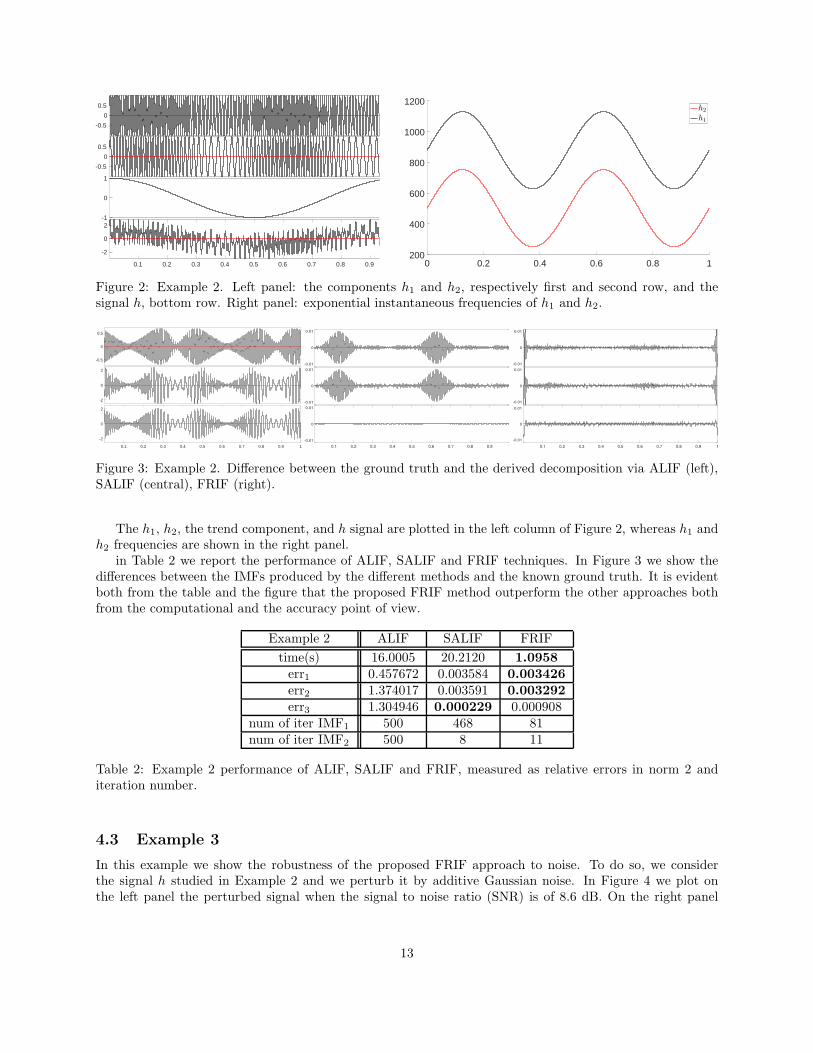
Figure 2: Example 2. Left panel: the components h1 and h2, respectively first and second row, and thesignal h, bottom row. Right panel: exponential instantaneous frequencies of h1 and h2.

-0.5

0

0.5

-2

0

2

0.1 0.2 0.3 0.4 0.5 0.6 0.7 0.8 0.9 1

-2

0

2

-0.01

0

0.01

-0.01

0

0.01

0.1 0.2 0.3 0.4 0.5 0.6 0.7 0.8 0.9 1

-0.01

0

0.01

-0.01

0

0.01

-0.01

0

0.01

0.1 0.2 0.3 0.4 0.5 0.6 0.7 0.8 0.9 1

-0.01

0

0.01

Figure 3: Example 2. Difference between the ground truth and the derived decomposition via ALIF (left),SALIF (central), FRIF (right).

The h1, h2, the trend component, and h signal are plotted in the left column of Figure 2, whereas h1 andh2 frequencies are shown in the right panel.

in Table 2 we report the performance of ALIF, SALIF and FRIF techniques. In Figure 3 we show thedifferences between the IMFs produced by the different methods and the known ground truth. It is evidentboth from the table and the figure that the proposed FRIF method outperform the other approaches bothfrom the computational and the accuracy point of view.

Example 2 ALIF SALIF FRIF

time(s) 16.0005 20.2120 1.0958err1 0.457672 0.003584 0.003426err2 1.374017 0.003591 0.003292err3 1.304946 0.000229 0.000908

num of iter IMF1 500 468 81num of iter IMF2 500 8 11

Table 2: Example 2 performance of ALIF, SALIF and FRIF, measured as relative errors in norm 2 anditeration number.

4.3 Example 3

In this example we show the robustness of the proposed FRIF approach to noise. To do so, we considerthe signal h studied in Example 2 and we perturb it by additive Gaussian noise. In Figure 4 we plot onthe left panel the perturbed signal when the signal to noise ratio (SNR) is of 8.6 dB. On the right panel

13

0 0.2 0.4 0.6 0.8 1-4

-2

0

2

4noisy signalnoiseless signal

-1

0

1

-1

0

1

-1

0

1

0.1 0.2 0.3 0.4 0.5 0.6 0.7 0.8 0.9 1-1

0

1

Figure 4: Example 3. Left panel, the noisy signal compared with the noiseless signal h defined in Example2. The SNR is around 8.6 dB. Right panel, the IMF decomposition derived by FRIF.

0 0.2 0.4 0.6 0.8 1-10

-5

0

5

10noisy signalnoiseless signal -5

0

5

-2

0

2

-1

0

1

-1

0

1

-1

0

1

0.1 0.2 0.3 0.4 0.5 0.6 0.7 0.8 0.9 1

-101

Figure 5: Example 3. Left panel, the noisy signal with SNR around 1.3 dB compared with the noiselesssignal h of Example 2. Right panel, the corresponding FRIF decomposition compared with the ground truth.

we report the decomposition produced by FRIF. It is evident that the method can separate properly therandom perturbation in the first row, from the deterministic components in the following three rows.

This result is confirmed even if we increase the SNR to 1.3 dB, left panel of Figure 5. It is evident fromthis figure that this level of noise is quite high. Nevertheless FRIF method proves to be able still to separatethe deterministic signal from the additive Gaussian contribution, as shown in the left panel of Figure 5.

4.4 Example 4

We conclude the numerical section with an example based on a real life signal. We consider the recording ofthe sound emitted by a bat, shown in the left panel of Figure 6. In the central panel, we show the associatedtime-frequency plot obtained using the IMFogram [7]. From this plot we observe that this signal appearsto contain three main simple oscillatory components which present rapid changes in frequencies. Thoseare classical examples of the so called chirps. By using a curve extraction method, it is possible to derivefrom the IMFogram the instantaneous frequency curves plotted in the right panel of Figure 6. As brieflymentioned earlier, the identification of these instantaneous frequency curves is of fundamental importancefor the proper functioning of FRIF, but it is also a research topic per se. In this work, we assume that theycan be computed accurately and we postpone the analysis of how to compute them in a robust and accurateway to future works.

By leveraging on the extracted curves, we run FRIF algorithm and derive the decomposition shown inthe left most panel of Figure 7. The first three IMFs produced correspond to the three main chirps observedin the IMFogram, which is depicted in the central panel of Figure 6. This is confirmed by running IMFogramseparately on the first three IMFs produced by FRIF. The results are shown in the rightmost 3 panels ofFigure 7. From these plots it becomes clear that the algorithm is able to separate in a clean way the three

14

1 2 3 4 5 6

-0.2

-0.15

-0.1

-0.05

0

0.05

0.1

1 2 3 4 5 60

5

10

15

20

25

30

Figure 6: Example 4. Left panel, sound produced by a bat. Central panel, the corresponding IMFogramtime-frequency plot. Right panel, instantaneous frequency curves inferred from the IMFogram plot.

-0.05

0

0.05

-0.1

0

0.1

-0.05

0

0.05

1 2 3 4 5 6

0

5

1010

-3

Figure 7: Example 4. Left most panel, IMF decomposition produced by FRIF. From central left to rightmost panel, the IMFogram time-frequency plots associated with the first, second and third row in the FRIFdecomposition, respectively.

chirps contained in the signal.

5 Conclusions

Following the success of the Empirical Mode Decomposition (EMD) method for the decomposition of non-stationary signals, and given that its mathematical understanding is still very limited, in recent years theIterative Filtering (IF) first, and then the Adaptive Local Iterative Filtering (ALIF) have been proposed.They inherit the same structure of EMD, but rely on convolution for the computation of the signal movingaverage. On the one hand, the mathematical understanding of IF is now pretty advanced, this includeits acceleration in what is called Fast Iterative Filtering (FIF) and its complete convergence analysis. Onthe other hand, IF proved to be limited in separating, in a physically meaningful way, components whichexhibit quick changes in their frequencies, like chirps or whistles. For this reason ALIF was proposedas a generalization of IF which overcome the limitations that are present in IF. However, even thoughsome advances have been obtained in recent years, the theoretical understanding of ALIF is far from beingcomplete. In particular, it is not yet clear under which assumptions it is possible to guarantee a priori itsconvergence.

For this reason, in this work we introduced the Resampled Iterative Filtering (RIF), and, in the discretesetting, the Stable Adaptive Local Iterative Filtering (SALIF) and the Fast Resampled Iterative Filtering(FRIF), that are capable of decomposing non-stationary signals into simple oscillatory components, even inpresence of fast changes in their instantaneous frequencies, like in chirps. We have analyzed them from a the-oretical stand point, showing, among other things, that it is possible to guarantee a priori their convergence.Furthermore, we have tested them using several artificial and real life examples.

More is yet to be said about the argument. In particular, all these methods are dependent on thecomputation of a length function ℓ(x) which is, de facto, the reciprocal of the instantaneous frequency curveassociated with each component contained in the signal. This function is required to guide the aforementionedmethods, including ALIF itself, in the extraction of physically meaningful IMFs. The identification ofinstantaneous frequency curves associated with each component contained in a given signal is a researchtopic per se, and it is out of the scope of the present work. This is why we plan to study this problem infuture works.

15

Another open problem regards the selection of an optimal stopping criterion and its tuning to be usedin this kind of methods. The stopping criterion implemented can influence consistently the performance ofthese techniques. We plan to work in this direction in the future.

Finally, we plan to work on the extension of the proposed techniques to handle multidimensional andmultivariate signals.

Acknowledgements

The authors are members of the Italian “Gruppo Nazionale di Calcolo Scientifico” (GNCS) of the IstitutoNazionale di Alta Matematica “Francesco Severi” (INdAM). AC thanks the Italian Space Agency, for thefinancial support under the contract ASI - LIMADOU scienza+n◦ 2020-31-HH.0, and the ISSI-BJ project“the electromagnetic data validation and scientific application research based on CSES satellite”.

References

[1] X. An. Local rub-impact fault diagnosis of a rotor system based on adaptive local iterative filtering.Transactions of the Institute of Measurement and Control, 39(5):748–753, 2017.

[2] X. An, C. Li, and F. Zhang. Application of adaptive local iterative filtering and approximate entropyto vibration signal denoising of hydropower unit. Journal of Vibroengineering, 18(7):4299–4311, 2016.

[3] X. An and L. Pan. Wind turbine bearing fault diagnosis based on adaptive local iterative filteringand approximate entropy. Proceedings of the Institution of Mechanical Engineers, Part C: Journal ofMechanical Engineering Science, 231(17):3228–3237, 2017.

[4] X. An, W. Yang, and X. An. Vibration signal analysis of a hydropower unit based on adaptive localiterative filtering. Proceedings of the Institution of Mechanical Engineers, Part C: Journal of MechanicalEngineering Science, 231(7):1339–1353, 2017.

[5] X. An, H. Zeng, and C. Li. Demodulation analysis based on adaptive local iterative filtering for bearingfault diagnosis. Measurement, 94:554–560, 2016.

[6] G. Barbarino and A. Cicone. Conjectures on spectral properties of alif algorithm, 2021.arXiv:2009.00582.

[7] P. Barbe, A. Cicone, W. Suet Li, and H. Zhou. Time-frequency representation of nonstationary signals:the imfogram. Pure and Applied Functional Analysis, 2021.

[8] A. Cicone. Iterative filtering as a direct method for the decomposition of nonstationary signals. Nu-merical Algorithms, pages 1–17, 2020.

[9] A. Cicone and P. Dell’Acqua. Study of boundary conditions in the iterative filtering method for the de-composition of nonstationary signals. Journal of Computational and Applied Mathematics, 373:112248,2020.

[10] A. Cicone, C. Garoni, and S. Serra-Capizzano. Spectral and convergence analysis of the discrete alifmethod. Linear Algebra and its Applications, 580:62–95, 2019.

[11] A. Cicone, W. S. Li, and H. Zhou. New theoretical insights in the decomposition and time-frequencyrepresentation of nonstationary signals: the imfogram algorithm. preprint, 2021.

[12] A. Cicone, J. Liu, and H. Zhou. Adaptive local iterative filtering for signal decomposition and instan-taneous frequency analysis. Applied and Computational Harmonic Analysis, 41(2):384–411, 2016.

16

[13] A. Cicone and H.-T. Wu. Convergence analysis of adaptive locally iterative filtering and sift method.submitted, 2021.

[14] A. Cicone and H. Zhou. Numerical analysis for iterative filtering with new efficient implementationsbased on fft. Numerische Mathematik, 147(1):1–28, 2021.

[15] C. Huang, L. Yang, and Y. Wang. Convergence of a convolution-filtering-based algorithm for empiricalmode decomposition. Advances in Adaptive Data Analysis, 1(04):561–571, 2009.

[16] N. E. Huang. Introduction to the hilbert–huang transform and its related mathematical problems.Hilbert–Huang transform and its applications, pages 1–26, 2014.

[17] N. E. Huang, Z. Shen, S. R. Long, M. C. Wu, H. H. Shih, Q. Zheng, N.-C. Yen, C. C. Tung, and H. H.Liu. The empirical mode decomposition and the hilbert spectrum for nonlinear and non-stationarytime series analysis. Proceedings of the Royal Society of London. Series A: mathematical, physical andengineering sciences, 454(1971):903–995, 1998.

[18] S. J. Kim and H. Zhou. A multiscale computation for highly oscillatory dynamical systems usingempirical mode decomposition (emd)–type methods. Multiscale Modeling & Simulation, 14(1):534–557,2016.

[19] Y. Li, X. Wang, Z. Liu, X. Liang, and S. Si. The entropy algorithm and its variants in the fault diagnosisof rotating machinery: A review. IEEE Access, 6:66723–66741, 2018.

[20] L. Lin, Y. Wang, and H. Zhou. Iterative filtering as an alternative algorithm for empirical modedecomposition. Advances in Adaptive Data Analysis, 1(04):543–560, 2009.

[21] I. Mitiche, G. Morison, A. Nesbitt, M. Hughes-Narborough, B. G. Stewart, and P. Boreham. Classifi-cation of partial discharge signals by combining adaptive local iterative filtering and entropy features.Sensors, 18(2):406, 2018.

[22] M. Piersanti, M. Materassi, A. Cicone, L. Spogli, H. Zhou, and R. G. Ezquer. Adaptive local itera-tive filtering: A promising technique for the analysis of nonstationary signals. Journal of GeophysicalResearch: Space Physics, 123(1):1031–1046, 2018.

[23] R. Sharma, R. B. Pachori, and A. Upadhyay. Automatic sleep stages classification based on iterativefiltering of electroencephalogram signals. Neural Computing and Applications, 28(10):2959–2978, 2017.

[24] A. Stallone, A. Cicone, and M. Materassi. New insights and best practices for the successful use ofempirical mode decomposition, iterative filtering and derived algorithms. Scientific Reports, 10:15161,2020.

[25] M. E. Torres, M. A. Colominas, G. Schlotthauer, and P. Flandrin. A complete ensemble empirical modedecomposition with adaptive noise. In 2011 IEEE international conference on acoustics, speech andsignal processing (ICASSP), pages 4144–4147. IEEE, 2011.

[26] N. Ur Rehman and D. P. Mandic. Filter bank property of multivariate empirical mode decomposition.IEEE transactions on signal processing, 59(5):2421–2426, 2011.

[27] H.-T. Wu. Current state of nonlinear-type time-frequency analysis and applications to high-frequencybiomedical signals. Current Opinion in Systems Biology, 23:8–21, 2020.

[28] Z. Wu and N. E. Huang. Ensemble empirical mode decomposition: a noise-assisted data analysismethod. Advances in adaptive data analysis, 1(01):1–41, 2009.

[29] D. Yang, B. Wang, G. Cai, and J. Wen. Oscillation mode analysis for power grids using adaptive localiterative filter decomposition. International Journal of Electrical Power & Energy Systems, 92:25–33,2017.

17

[30] J.-R. Yeh, J.-S. Shieh, and N. E. Huang. Complementary ensemble empirical mode decomposition: Anovel noise enhanced data analysis method. Advances in adaptive data analysis, 2(02):135–156, 2010.

[31] J. Zheng, J. Cheng, and Y. Yang. Partly ensemble empirical mode decomposition: An improved noise-assisted method for eliminating mode mixing. Signal Processing, 96:362–374, 2014.

18