Scholars' Mine Scholars' Mine

Masters Theses Student Theses and Dissertations

Summer 2019

Controlled switching in Kalman filtering and iterative learning Controlled switching in Kalman filtering and iterative learning

controls controls

He Li

Follow this and additional works at: https://scholarsmine.mst.edu/masters_theses

Part of the Artificial Intelligence and Robotics Commons, Mechanical Engineering Commons, and the

Robotics Commons

Department: Department:

Recommended Citation Recommended Citation Li, He, "Controlled switching in Kalman filtering and iterative learning controls" (2019). Masters Theses. 8078. https://scholarsmine.mst.edu/masters_theses/8078

This thesis is brought to you by Scholars' Mine, a service of the Missouri S&T Library and Learning Resources. This work is protected by U. S. Copyright Law. Unauthorized use including reproduction for redistribution requires the permission of the copyright holder. For more information, please contact scholarsmine@mst.edu.

CONTROLLED SWITCHING IN KALMAN FILTERING AND ITERATIVE

LEARNING CONTROL

by

HE LI

A THESIS

Presented to the Graduate Faculty of the

MISSOURI UNIVERSITY OF SCIENCE AND TECHNOLOGY

In Partial Fulfillment of the Requirements for the Degree

MASTER OF SCIENCE

in

MECHANICAL ENGINEERING

2019

Approved by

Dr. Douglas A. Bristow, AdvisorDr. Robert G. Landers, Co-Advisor

Dr. S. N. Balakrishnan

Copyright 2019

HE LI

All Rights Reserved

iii

PUBLICATION THESIS OPTION

This thesis consists of the following two articles which have been published, or will

be submitted for publication as follows:

Paper I: Pages 24-51 have been published on Precision Engineering Journal.

Paper II: Pages 52-88 are intended for submission to IEEETransactions onAutomatic

Control Journal.

iv

ABSTRACT

Switching is not an uncommon phenomenon in practical systems and processes,

for examples, power switches opening and closing, transmissions lifting from low gear

to high gear, and air planes crossing different layers in air. Switching can be a disaster

to a system since frequent switching between two asymptotically stable subsystems may

result in unstable dynamics. On the contrary, switching can be a benefit to a system since

controlled switching is sometimes imposed by the designers to achieve desired performance.

This encourages the study of system dynamics and performance when undesired switching

occurs or controlled switching is imposed. In this research, the controlled switching

is applied to an estimation process and a multivariable Iterative Learning Control (ILC)

system, and system stability as well as system performance under switching are investigated.

The first article develops a controlled switching strategy for the estimation of a temporal

shift in a Laser Tracker (LT). For some reason, the shift cannot be measured at all time.

Therefore, a model-based predictor is adopted for estimation when the measurement is not

available, and a Kalman Filter (KF) is used to update the estimate when the measurement is

available. With the proposed method, the estimation uncertainty is always bounded within

two predefined boundaries. The second article develops a controlled switching method for

multivariable ILC systems where only partial outputs are measured at a time. Zero tracking

error cannot be achieved for such systems using standard ILC due to incomplete knowledge

of the outputs. With the developed controlled switching, all the outputs are measured in a

sequential order, and, with each currently-measured output, the standard ILC is executed.

Conditions under which zero convergent tracking error is accomplished with the proposed

method are investigated. The proposed method is finally applied to solving a multi-agent

coordination problem.

v

ACKNOWLEDGMENTS

First and foremost, I would like to thank my advisors, Dr. Douglas A. Bristow

and Dr. Robert G. Landers, for their continuous support and guidance toward my research

and for their concerns for my professional development. Their well beings and optimism

are appreciated which have helped me get through every frustration encountered in my

research. I will miss thinking together in our regular meetings and will remember their

constant confidences in me.

I also want to thank Dr. John Singler for his insightful suggestions on my Iterative

Learning Control research, and Dr. Balakrishnan for his wise comments on my thesis. My

first control class at Missouri S & T was taken with Dr. Balakrishnan, and I appreciate

his kindness in discussing with me many control topics that I did not know.

Thank also the past and current members in the PMC lab. It was a rewarding and

enjoyable experience staying with them, both inside and outside the lab. I will miss the fun

times making jokes with Le Ma, Patrick Bazolli, Theodore Ebbesmeyer on Michelle.

I would also like to gratefully acknowledge those agencies funding my research,

including National Science Foundation (CMMI-1335340), the Department of the Army

through the Digital Manufacturing and Design Innovation Institute (DMDII15-07-01), the

Center for Aerospace Manufacturing Technologies and the Intelligent System Center at the

Missouri University of Science and Technology.

Last, but certainly not least, I must thank my family and my friends. Thanks to my

parents Quanfeng and Cheng for their constant support, concerns and love. They are the

most important persons to me in this world. Thanks to my friends Hongzhao, Xingyue and

Xuanyi, for taking care of my parents when I was not at home. Thanks to my friends, Adam

Lewis, Le Ma, Muchen Sun, Yifu Long and Bin Sun, for all the fun times. Thanks to all

my friends here in Rolla and in china. Their support has always been important to me.

vi

TABLE OF CONTENTS

Page

PUBLICATION THESIS OPTION . . . . . . . . . . . . . . . . . . . . . . . . . . . . . . . . . . . . . . . . . . . . . . iii

ABSTRACT . . . . . . . . . . . . . . . . . . . . . . . . . . . . . . . . . . . . . . . . . . . . . . . . . . . . . . . . . . . . . . . . . . iv

ACKNOWLEDGMENTS . . . . . . . . . . . . . . . . . . . . . . . . . . . . . . . . . . . . . . . . . . . . . . . . . . . . . . v

LIST OF ILLUSTRATIONS . . . . . . . . . . . . . . . . . . . . . . . . . . . . . . . . . . . . . . . . . . . . . . . . . . . . x

LIST OF TABLES . . . . . . . . . . . . . . . . . . . . . . . . . . . . . . . . . . . . . . . . . . . . . . . . . . . . . . . . . . . . . xii

SECTION

1. INTRODUCTION. . . . . . . . . . . . . . . . . . . . . . . . . . . . . . . . . . . . . . . . . . . . . . . . . . . . . . . . . . 1

2. KALMAN FILTERING. . . . . . . . . . . . . . . . . . . . . . . . . . . . . . . . . . . . . . . . . . . . . . . . . . . . . 3

2.1. BACKGROUND . . . . . . . . . . . . . . . . . . . . . . . . . . . . . . . . . . . . . . . . . . . . . . . . . . . . . . . . . . . . . . . . . 3

2.2. KALMAN FILTERING BASICS . . . . . . . . . . . . . . . . . . . . . . . . . . . . . . . . . . . . . . . . . . . . . . . 3

3. ITERATIVE LEARNING CONTROL. . . . . . . . . . . . . . . . . . . . . . . . . . . . . . . . . . . . . . . . 6

3.1. BACKGROUND . . . . . . . . . . . . . . . . . . . . . . . . . . . . . . . . . . . . . . . . . . . . . . . . . . . . . . . . . . . . . . . . . 6

3.2. ILC BASICS . . . . . . . . . . . . . . . . . . . . . . . . . . . . . . . . . . . . . . . . . . . . . . . . . . . . . . . . . . . . . . . . . . . . . 8

3.3. REPRESENTATIONS OF ILC SYSTEMS. . . . . . . . . . . . . . . . . . . . . . . . . . . . . . . . . . . . . 10

3.3.1. Time-domain Lifted System Representation . . . . . . . . . . . . . . . . . . . . . . . . . . . 10

3.3.2. Frequency-Domain Representation . . . . . . . . . . . . . . . . . . . . . . . . . . . . . . . . . . . . . 12

3.4. ILC PERFORMANCE. . . . . . . . . . . . . . . . . . . . . . . . . . . . . . . . . . . . . . . . . . . . . . . . . . . . . . . . . . . 13

3.4.1. Convergence and Asymptotic Convergence . . . . . . . . . . . . . . . . . . . . . . . . . . . . 13

3.4.2. Monotonic Convergence . . . . . . . . . . . . . . . . . . . . . . . . . . . . . . . . . . . . . . . . . . . . . . . . 15

vii

3.4.3. Robustness . . . . . . . . . . . . . . . . . . . . . . . . . . . . . . . . . . . . . . . . . . . . . . . . . . . . . . . . . . . . . . . 16

3.4.4. Considerations of Noise and Non-repeatable Errors . . . . . . . . . . . . . . . . . . . 17

3.5. ILC DESIGN . . . . . . . . . . . . . . . . . . . . . . . . . . . . . . . . . . . . . . . . . . . . . . . . . . . . . . . . . . . . . . . . . . . . . 19

3.5.1. PD-Type Design . . . . . . . . . . . . . . . . . . . . . . . . . . . . . . . . . . . . . . . . . . . . . . . . . . . . . . . . . 19

3.5.2. Model-Inversion Design. . . . . . . . . . . . . . . . . . . . . . . . . . . . . . . . . . . . . . . . . . . . . . . . . 20

3.5.3. Linearly Quadratic Optimization . . . . . . . . . . . . . . . . . . . . . . . . . . . . . . . . . . . . . . . 21

3.5.4. Recommendations for ILC Design . . . . . . . . . . . . . . . . . . . . . . . . . . . . . . . . . . . . . 22

PAPER

I. A SWITCHEDESTIMATIONSTRATEGYBASEDONKALMANFILTERINGFOR COMPENSATING LASER TRACKER ADM SHIFT. . . . . . . . . . . . . . . . . . . . . 24

ABSTRACT . . . . . . . . . . . . . . . . . . . . . . . . . . . . . . . . . . . . . . . . . . . . . . . . . . . . . . . . . . . . . . . . . . . . . . . . . . . . 24

1. INTRODUCTION . . . . . . . . . . . . . . . . . . . . . . . . . . . . . . . . . . . . . . . . . . . . . . . . . . . . . . . . . . . . . . . 25

2. KALMAN FILTER AND MODIFIED KALMAN FILTER. . . . . . . . . . . . . . . . . . . 28

2.1. KALMAN FILTER. . . . . . . . . . . . . . . . . . . . . . . . . . . . . . . . . . . . . . . . . . . . . . . . . . . . . . 29

2.2. MODIFIED KALMAN FILTER . . . . . . . . . . . . . . . . . . . . . . . . . . . . . . . . . . . . . . . 30

3. SWITCHED ESTIMATION STRATEGY. . . . . . . . . . . . . . . . . . . . . . . . . . . . . . . . . . . . . . 31

3.1. PROPAGATION OF MKF ESTIMATION ERROR COVARIANCE 32

3.2. SWITCHED ESTIMATION STRATEGY . . . . . . . . . . . . . . . . . . . . . . . . . . . . . 34

3.3. SELECT U AND L . . . . . . . . . . . . . . . . . . . . . . . . . . . . . . . . . . . . . . . . . . . . . . . . . . . . . 36

3.4. RTS SMOOTHING . . . . . . . . . . . . . . . . . . . . . . . . . . . . . . . . . . . . . . . . . . . . . . . . . . . . . 38

4. EXPERIMENTAL VALIDATION . . . . . . . . . . . . . . . . . . . . . . . . . . . . . . . . . . . . . . . . . . . . . . 39

4.1. ADM SHIFT MODEL . . . . . . . . . . . . . . . . . . . . . . . . . . . . . . . . . . . . . . . . . . . . . . . . . . 40

4.2. EXPERIMENTAL SETUP . . . . . . . . . . . . . . . . . . . . . . . . . . . . . . . . . . . . . . . . . . . . . 42

4.3. PARAMETER SELECTION . . . . . . . . . . . . . . . . . . . . . . . . . . . . . . . . . . . . . . . . . . . 42

4.3.1. Initial Estimation Uncertainty . . . . . . . . . . . . . . . . . . . . . . . . . . . . . . . 42

4.3.2. Upper Bound U and Lower Bound L . . . . . . . . . . . . . . . . . . . . . . . . 43

viii

4.4. EXPERIMENTAL IMPLEMENTATION AND RESULTS . . . . . . . . . . 45

5. SUMMARY AND CONCLUSIONS . . . . . . . . . . . . . . . . . . . . . . . . . . . . . . . . . . . . . . . . . . . 48

ACKNOWLEDGEMENTS . . . . . . . . . . . . . . . . . . . . . . . . . . . . . . . . . . . . . . . . . . . . . . . . . . . . . . . . . . . . 49

REFERENCES . . . . . . . . . . . . . . . . . . . . . . . . . . . . . . . . . . . . . . . . . . . . . . . . . . . . . . . . . . . . . . . . . . . . . . . . . 49

II. ITERATIVE LEARNING CONTROL FOR MULTIVARIABLE SYSTEMSWITH SWITCHING OUTPUTS AND APPLICATION TO MULTI-AGENTCOORDINATION . . . . . . . . . . . . . . . . . . . . . . . . . . . . . . . . . . . . . . . . . . . . . . . . . . . . . . . . . 52

ABSTRACT . . . . . . . . . . . . . . . . . . . . . . . . . . . . . . . . . . . . . . . . . . . . . . . . . . . . . . . . . . . . . . . . . . . . . . . . . . . . 52

1. INTRODUCTION . . . . . . . . . . . . . . . . . . . . . . . . . . . . . . . . . . . . . . . . . . . . . . . . . . . . . . . . . . . . . . . 53

2. PROBLEM FORMULATION. . . . . . . . . . . . . . . . . . . . . . . . . . . . . . . . . . . . . . . . . . . . . . . . . . . 55

2.1. MATRIXREPRESENTATIONOFMULTIVARIABLE ILCSYS-TEMS . . . . . . . . . . . . . . . . . . . . . . . . . . . . . . . . . . . . . . . . . . . . . . . . . . . . . . . . . . . . . . . . . . . . 55

2.2. NONZERO-ERROR CONVERGENCE PROBLEM FOR A SPE-CIAL CLASS OF MULTIVARIABLE SYSTEMS . . . . . . . . . . . . . . . . . . . . 61

3. ILC-BASED SWITCHING ALGORITHM .. . . . . . . . . . . . . . . . . . . . . . . . . . . . . . . . . . . 62

3.1. SWICHING ALGORITHM .. . . . . . . . . . . . . . . . . . . . . . . . . . . . . . . . . . . . . . . . . . . 62

3.2. ITERATION DOMAIN CONVERGENCE . . . . . . . . . . . . . . . . . . . . . . . . . . . . 63

3.3. SWITCH DOMAIN CONVERGENCE . . . . . . . . . . . . . . . . . . . . . . . . . . . . . . . . 65

3.4. SINGLE INPUT UPDATE SWITCHING ALGORITHM .. . . . . . . . . . . 67

4. LEARNING MATRIX DESIGN FOR THE SWITCHING ALGORITHM .. 68

4.1. PLANT INVERSION DESIGN . . . . . . . . . . . . . . . . . . . . . . . . . . . . . . . . . . . . . . . . 68

4.2. LINEARLY QUADRATIC OPTIMIZATION DESIGN . . . . . . . . . . . . . . 69

5. APPLICATION TO MULTI-AGENT COORDINATION . . . . . . . . . . . . . . . . . . . . . 73

5.1. NOTATIONS USED IN MULTI-AGENT SYSTEMS . . . . . . . . . . . . . . . . 73

5.2. LINEARMULTI-AGENTSYSTEMSANDCONSENSUSPROB-LEM.. . . . . . . . . . . . . . . . . . . . . . . . . . . . . . . . . . . . . . . . . . . . . . . . . . . . . . . . . . . . . . . . . . . . . 74

5.3. RELATIVE TRAJECTORY TRACKING USING RELATIVE-INFORMATION FEEDBACK CONTROL. . . . . . . . . . . . . . . . . . . . . . . . . . . . 75

ix

5.4. GLOBAL TRAJECTORY TRACKING COMBING FEEDBACKAND FEEDFORWARD CONTROL . . . . . . . . . . . . . . . . . . . . . . . . . . . . . . . . . . . 76

5.5. SIMULATION STUDY . . . . . . . . . . . . . . . . . . . . . . . . . . . . . . . . . . . . . . . . . . . . . . . . . 78

5.5.1. Relative Trajectory Tracking Using Feedback Control . . . . . 79

5.5.2. Global Trajectory Tracking Using SILC . . . . . . . . . . . . . . . . . . . . 80

5.5.3. Global Trajectory Tracking Using Single Input UpdateSILC . . . . . . . . . . . . . . . . . . . . . . . . . . . . . . . . . . . . . . . . . . . . . . . . . . . . . . . . . . 81

6. SUMMARY AND CONCLUSIONS . . . . . . . . . . . . . . . . . . . . . . . . . . . . . . . . . . . . . . . . . . . 83

APPENDIX . . . . . . . . . . . . . . . . . . . . . . . . . . . . . . . . . . . . . . . . . . . . . . . . . . . . . . . . . . . . . . . . . . . . . . . . . . . . . 84

REFERENCES . . . . . . . . . . . . . . . . . . . . . . . . . . . . . . . . . . . . . . . . . . . . . . . . . . . . . . . . . . . . . . . . . . . . . . . . . 87

SECTION

4. SUMMARY AND CONCLUSIONS . . . . . . . . . . . . . . . . . . . . . . . . . . . . . . . . . . . . . . . . . 89

REFERENCES . . . . . . . . . . . . . . . . . . . . . . . . . . . . . . . . . . . . . . . . . . . . . . . . . . . . . . . . . . . . . . . . 91

VITA . . . . . . . . . . . . . . . . . . . . . . . . . . . . . . . . . . . . . . . . . . . . . . . . . . . . . . . . . . . . . . . . . . . . . . . . . 94

x

LIST OF ILLUSTRATIONS

Figure Page

SECTION

3.1. Illustration of iterative learning control in time domain and iteration domain. . . . 7

3.2. Illustration of a plug-in type ILC system. . . . . . . . . . . . . . . . . . . . . . . . . . . . . . . . . . . . . . . . . . . . 10

3.3. Plug-in type ILC system incorporating measurement noise and non-repeatabledisturbances. . . . . . . . . . . . . . . . . . . . . . . . . . . . . . . . . . . . . . . . . . . . . . . . . . . . . . . . . . . . . . . . . . . . . . . . . . . 18

PAPER I

1. (a) Multiple-targets measurement experimental setup (A ≈ 990 mm, B ≈ 1954mm, C ≈ 2950 mm and D ≈ 3968 mm are distances from the LT to targets1, 2, 3 and 4, respectively). (b) Resulting distance variation when measuringeach target. . . . . . . . . . . . . . . . . . . . . . . . . . . . . . . . . . . . . . . . . . . . . . . . . . . . . . . . . . . . . . . . . . . . . . . . . . . . . 26

2. Illustration of the Switched Estimation strategy.. . . . . . . . . . . . . . . . . . . . . . . . . . . . . . . . . . . . 35

3. (a) Experimental setup for system identification and switched estimation im-plementation experiments. (b) ADM shift measurement from system identifi-cation experiment. . . . . . . . . . . . . . . . . . . . . . . . . . . . . . . . . . . . . . . . . . . . . . . . . . . . . . . . . . . . . . . . . . . . . 41

4. Selection map that describes the effect of U and L on ρ. . . . . . . . . . . . . . . . . . . . . . . . . . . 44

5. Propagation of the estimation uncertainty P+k obtained from SE algorithm andtime duration of each stage (k0 = 9, k1 = 129, k2 = 138) for the first 300 timeinstants. . . . . . . . . . . . . . . . . . . . . . . . . . . . . . . . . . . . . . . . . . . . . . . . . . . . . . . . . . . . . . . . . . . . . . . . . . . . . . . . 45

6. (a) ADM shift measurements, ADM shift estimates given by SE algorithm andthat given by RTSS for the entire time history. The unit of X-axis is hr whichis recorded in real time. (b) ADM shift estimation uncertainty given by SEalgorithm and that given by RTSS for the first 150 time instants. . . . . . . . . . . . . . . . . . 46

7. Radial distancemeasurements of SMR1, 2 and 3 and their compensated valuesbased on SE strategy and RTSS estimation. . . . . . . . . . . . . . . . . . . . . . . . . . . . . . . . . . . . . . . . . 47

PAPER II

1. Graphical representation of topology relationship of a three-agent system. . . . . . . . 74

2. Illustration of desired relative trajectory and global trajectory for simulationstudy. . . . . . . . . . . . . . . . . . . . . . . . . . . . . . . . . . . . . . . . . . . . . . . . . . . . . . . . . . . . . . . . . . . . . . . . . . . . . . . . . . . 79

xi

3. Relative trajectory tracking using relative-information feedback control. . . . . . . . . . 80

4. Actual trajectories of each agent for the first three switches when SILC algo-rithm is applied. . . . . . . . . . . . . . . . . . . . . . . . . . . . . . . . . . . . . . . . . . . . . . . . . . . . . . . . . . . . . . . . . . . . . . . 81

5. Actual trajectories of each agent for the 1st, 2nd, 3rd, 13th, 19th and the 30thswitch when the single input update SILC algorithm is applied. . . . . . . . . . . . . . . . . . . 82

6. Error evolution in the swich domain when single input update SILC applies. . . . . 83

xii

LIST OF TABLES

Table Page

PAPER I

1. Identified model parameters.. . . . . . . . . . . . . . . . . . . . . . . . . . . . . . . . . . . . . . . . . . . . . . . . . . . . . . . . . 41

2. Maximum variation of radial distance measurements of SMR 1, 2 and 3,maximum variation and 2σ value of their compensated values. . . . . . . . . . . . . . . . . . . . 47

SECTION

1. INTRODUCTION

Switching is commonly observed in many systems and processes, for instance,

vehicle transmission systems transitioning from low gear to high gear, light switches turning

on and off, dynamics changing when airplane crossing different layers in air, and controller

switching for a robot from position control to force control etc. Depending on sources of

occurrence, switching may occur as the result of the nature of a process, or is intentionally

created by a designer. The occurrence of switching could be a disaster to the system. For

example, when two asymptocially stable subsystems are switched between each other very

frequently, the resulting system may become unstable [1]. On the contrary, switching may

be a benefit to the system. For example, a single continuous feedback controller cannot

guarantee the asymptotic stability of an inverted pendulum. Asymptotic stability, however,

is possible by switching the controller between an ‘energy-injection’ based controller and

a locally linearized controller around the equilibrium point [1]. The performance of a

switched system also depends on the switching signal or reset mapping, a mechanism that

determineswhen and how the subsystems are switched. This thesis is devoted to studying the

switching behaviours in an estimation process and in mutivariable Iterative learning Control

(ILC) systems, and to designing proper switching signals to achieve desired estimation and

controlling performances.

Paper I develops a controlled switching strategy for the estimation of a temporal shift

in a measurement device known as a Laser Tracker (LT), and investigates the estimation

performance under switching. An LT can continuously measure a 3D point and is well

known for its high accuracy and fast data collection. However, some LTs currently in

service have temporal shift issues which contaminate the measurements [2]. In order to

2

eliminate this effect, the temporal shift needs to be measured or estimated. Due to the

conflict between normal operation and shift measurement, two estimators, i.e., a Kalman

Filter (KF) and a model-based predictor, are adopted for estimation. The KF is active for

estimation when the shift measurement is available, whereas the predictor is active when

the LT is in normal operation. A switching signal is designed to control the LT to be in

normal operation or to measure the shift. By appropriately designing the switching signal,

the estimation uncertainty is bounded within two predefined boundaries. This is essentially

the hysteresis switching with the two boundaries representing the switching surfaces.

In Paper II, controlled switching is designed for multivariable Iterative Learning

Control (ILC) systems where only partial output channels can be measured at a time. For

such systems, zero tracking error cannot be accomplished with the standard ILC due to

the incomplete knowledge of the outputs [3, 4]. In order to achieve zero tracking error,

a switching method is brought into the system such that the all the output channels are

measured but in a sequential order, and with each measured output channel, the standard

ILC is executed. It is shown in the paper that if the ILC controller and the switching signal

are properly designed, then zero tracking error would be achieved as the switching action

continues.

Since the foundations for Paper I and Paper II are Kalman Filtering (KF) and Iterative

Learning Control (ILC), the basics of KF and ILC are introduced in Section 2 and Section

3, respectively. The readers are suggested to have an overview of these sections before

proceeding to Paper I and Paper II, provided that they do not have previous knowledge in

the fields.

3

2. KALMAN FILTERING

2.1. BACKGROUND

Kalman Filtering (KF), since it was invented by R. E. Kalman [5] in 1960, has

grown as the most popular tool for optimal state estimation for non-stationary processes.

It has found applications in a wide range of areas such as navigation and control [6, 7],

target tracking [8], and data fusion [9] etc. The very first Kalman filtering paper [5]

investigated the optimal estimation problem for linear stochastic systems. Its nonlinear

version, known as the Extended Kalman Filter (EKF), investigated the optimal estimation

problem for nonlinear stochastic systems by linearizing the estimation process around

approximate points. Since the EKF relies heavily on linearization, high nonlinearities in

the system may deteriorate EKF performance. In order to deal with the situation where the

linearization fails, Unscented Kalman Filter (UFK) was developed [10]. Note that although

different versions of the Kalman filtering technique may have different algorithms, the basic

principles behind them are identical, i.e., the final estimation is acquired by trading off a

model predicted value and the measurement, along with which the estimation covariance is

minimized and given. In the rest of this section, we introduce the KF basics for discrete-time

linear systems, in the sense that this is the foundation for Paper I in this thesis. The readers

are referred to [11, 12] for details about EKF and UKF.

2.2. KALMAN FILTERING BASICS

Consider a Discrete-Time (DT) Linear-Time-Invariant (LTI) stochastic system

xk+1 = Fxk +Guk + w,

yk = Hxk + v,(2.1)

4

w ∼ (0,Q),

v ∼ (0,R),

where x denotes the system state, u the input, y the output, and w and v the process noise

and the measurement noise, respectively. The random variables w and v are assumed to

be Gaussian with the covariances Q and R, respectively, which provide the information

about how much the nominal model, i.e., when w = 0, is trusted and how accurate the

measurement is. The goal of KF is to obtain optimal estimation of xk , i.e., with minimized

uncertainty, using the stochastic information embedded in w and v. At each time instant

k, the KF estimation consists of two stages. The first stage is known as prediction, during

which the estimation is performed based on the nominal model and the estimate at the

previous one time step, i.e.,

x−k+1 = Fx+k +Guk, (2.2)

P−k+1 = FP+k FT +Q, (2.3)

where x− denotes the a priori estimate with the covariance P−, and x+ denotes the a

posteriori estimate with the covariance P+. The second stage is known as the correction

stage, during which the estimate obtained in the prediction stage x−k+1 is adapted by the

measurement yk+1 to produce the corrected estimate x+k+1, i.e.,

x+k+1 = x−k+1 +Kk+1(yk+1 −Hx−k+1) , (2.4)

Kk+1 = P−k+1HT [HP−k+1HT + R]−1 , (2.5)

P+k+1 = (I −Kk+1H)P−k+1 , (2.6)

where Kk+1 is the gain matrix or weighting matrix which balances the relative importance

between the measurement yk+1 and the a posteriori estimate x−k+1. The gain matrix Kk+1 is

obtained by minimizing the covariance P+k+1 as in a recursive least-mean-square filter [13],

5

and, thus, the name of optimal estimation is defined. Note that both the a priori estimate

x−k+1 and the a posteriori estimate x+k+1 are estimates of the state xk+1. However, due to the

incorporation of the measurement information into x+k+1, the uncertainty of x+k+1 is less than

that of x−k+1, and, thus, more trustful. The mathematical justification for this conclusion is

discussed in Paper I in this thesis.

The KF algorithm (2.2 - 2.6) is initialized by

x+0 = E[x0], P+0 = E[(x+0 − x0)2]. (2.7)

The choices of x+0 and P+0 depend on how much information is known priori about the

initial state of the system. A sufficient large P+0 is expected if not much trust is paid to x+0 .

Under certain conditions, the estimation uncertainty P+k will converge to some constant P+∞,

which is known as the steady-state estimation uncertainty. The convergence of P+k and the

converged value P+∞ rely only on Q and R. Although Q and R characterize the stochastic

properties of the process noise w and the measurement noise v, in practice, they are more

often used as tuning parameters to make a tradeoff between the smoothness of the estimate

and the transient performance of P+0 . If R weights greater than Q, then the estimation

has more confidence in the measurement, and, thus, the estimation is more noisy, but P+kconverges fast to P+∞. On the contrary, if Q weights larger than R, then the estimate x+k is

more smooth. In this case, however, P+k converges slower to P+∞, or even worse, P+k may

fail to converge if Q is too large. Note that the convergence of P+k and the converged value

P+∞ are independent of P+0 . However, the choice of P+0 affects the monotonicity of P+k . If

P+0 > P+∞, then monotonic decrease is achieved. Details on this aspect are discussed in

detail in Paper I in this thesis since this property is used to develop a KF-based switching

algorithm in the same paper.

6

3. ITERATIVE LEARNING CONTROL

3.1. BACKGROUND

The concept of Iterative Learning Control (ILC) appeared in academia in the early

1980s when a series of independent studies were published [14, 15, 16]. As its name

implies, ILC aims at improving the performance of systems which execute the same task for

multiple times. Common information are embedded into the history of previous executions

of the task, which can be learned by ILC to iteratively reduce the error. Although ILC was

initially invented for robotics manipulators [14, 15, 16], through years of development, ILC

finds its applications in a wide range of areas, such as wafer stage [17], inkjet printer [18],

nano-positioning system[19, 20], laser metal deposition [21], multi-agent coordination [22,

23], etc. For more applications and overview of ILC, the readers are referred to surveys

[24, 25],

In tracking a reference, the basic tracking performance of a system is typically

guaranteed by a feedback controller. When a task is executed formultipl times, the repeatable

disturbances, however, cannot be utilized by the feedback controller, which is a waste. ILC is

a feedforward control technique which is often built over the overall closed-loop framework.

The dynamics of an ILC system can be considered in two domains, i.e., the time domain

and the iteration domain, as is shown in Figure 3.1. The iteration-domain dynamics is

characterized by the axis perpendicular to the screen, whereas the time-domain dynamics

by that in the screen. An initial input u0[k] to the system results in the error in the initial

iteration, i.e, e0[k]. This error is then learned by ILC through a learning process, the result

of which is used to adapt the input u0[k] to generate the input in the next iteration, i.e.,

u1[k]. This process is repeated indefinitely until the error converges to some desired values.

7

Figure 3.1. Illustration of iterative learning control in time domain and iteration domain.

As for all iterative algorithms, convergence is the most important performance to

evaluate an ILC system. Lucky for us, through years of development, concepts and theories

regarding to convergence have been well established, including convergence, asymptotic

convergence and monotonic convergence. The other evaluations of an ILC system perfor-

mance include converged error, robustness and convergence rate. These performances may

contradict with each other, for instance, high robustness may be achieved in the price of

large converged error. In practice, therefore, tradeoffs are made among these performances

by tuning a learning function and a filtering function.

This section provides a literature review of ILC basics, performance evaluations

and ILC design, for instance, time-domain and frequency-domain representations of ILC

systems, key concepts such as convergence, asymptotic convergence and monotonic con-

vergence, as well as the conditions under which they are achieved. In the end, we offer some

practical considerations in ILC design and implementation. It is expected that this section

could provide basic understandings of ILC to the readers, and thus be helpful to guide the

readers through the second paper in this thesis.

8

3.2. ILC BASICS

Consider a Discrete-Time (DT) Single-Input-Single-Output (SISO) Linear-Time-

Invariant (LTI) dynamic system

y j[k] = P(z)u j[k] + d[k], (3.1)

where k denotes the time step, u and y respectively, denote the control input and system

output, d denotes the disturbance signal, P(z) denotes the system transfer function [24]

where z refers to the forward time-shift operator. The subscript j denotes the iteration

index and the absence of j in d[k] indicates that the disturbance is repeated over every

iteration. The system P(z) is assumed to be stable and have relative degree of 1. If it is

not stable, a feedback controller can be applied and P(z) would represent the closed-loop

dynamics in that case. It is emphasized here that P(z) maps an input sequence to an output

sequence, rather than mapping a single sample in the input sequence to another sample in

the output sequence. The repeated disturbance signal d[k] not only incorporates the output

disturbance, but captures the effects of repeated input disturbance and repeated nonzero

initial conditions as well. For instance, consider the system

x j[k + 1] = Ax j[k] + Bu j[k]

y j[k] = Cx j[k]. (3.2)

Substituting x[k + 1] = zx[k] into (3.2) and with some manipulations, we get

y j[k] = C(zI − A)−1B︸ ︷︷ ︸P(z)

u j[k] + CAkBx[0]︸ ︷︷ ︸d[k]

. (3.3)

Given a desired output yd[k], the tracking error in the j th iteration is

e j[k] = −P(z)u j[k] + δ[k], (3.4)

9

where δ[k] = yd[k] − d[k]. In practice, a repeated process contains finite time duration in

each iteration. Denote with N the length of time in each iteration. Then,

u j[k] = u j[0], u j[1], · · · , u j(N − 1),

e j[k] = e j[1], e j[2], · · · , e j(N),

δ[k] = δ[1], δ[2], · · · , δ(N),

where the one-step delay is caused by the one relative degree in P(z).

Iterative Learning Control is to modify the input u j iteration by iteration by learning

previous errors through an update algorithm. A widely used first-order ILC algorithm is

u j+1[k] = Q(z)(u j[k] + zL(z)e j[k]), (3.5)

or equivalently,

u j+1[k] = Q(z)(u j[k] + L(z)e j[k + 1]), (3.6)

where e j[k] = y j[k] − d[k], Q(z) is a filtering function to select learning bandwidth and

L(z) is a learning function. Most commonly, Q(z) is a low-pass filter since the repeatable

errors mainly distribute in the low-frequency range, whereas the modeling uncertainties and

the measurement noise mainly happen in the high-frequency range. It is reported in [20]

that a band-pass filter may have a better performance in the case that non-repeatable errors

occur in the low-frequency range due to nonlinearity.

In order to have an insight of how ILC is implemented on a real system, an illustration

of a plug-in type ILC is depicted in Figure 3.2, where G(z) denotes the plant to be controlled

and C(z) denotes a feedback controller. The controller C(z) guarantees a basic tracking

performance when the ILC is not in effective, whereas the ILC improves this tracking

performance iteratively. The ‘memory’ shown in Figure 3.2 stores the error signal and the

feedforward input from the j th iteration which are used for input update in the ( j + 1)th

10

Figure 3.2. Illustration of a plug-in type ILC system.

iteration. Ideally, the size of the ‘memory’ is N . In practice, however, the learning function

L(z) and the filtering function Q(z)might be non-causal, and, thus, the ‘memory’ size need

to be altered for implementation. For the system shown in Figure 3.2, if the ILC is disabled,

then

e j[k] = −P(z)u j[k] + S(z)(r[k] − d[k])︸ ︷︷ ︸δ[k]

, (3.7)

where

P(z) =G(z)

1 + G(z)C(z), S(z) =

11 + G(z)C(z)

. (3.8)

The tracking error is in the same form of the equation (3.4), and, thus, all ILC properties,

theories and designs apply.

3.3. REPRESENTATIONS OF ILC SYSTEMS

To facilitate the performance analysis and the design of the ILC system (3.1) and

(3.5), time-domain representations and frequency-domain representations are introduced.

3.3.1. Time-domain Lifted System Representation. The one-relative-degree DT

LTI transfer function P(z) can be expanded through long division as

P(z) = p1z−1 + p2z−2 + · · · + pN z−N + · · · , (3.9)

11

where the sequence pk∞k=1 refers to the weighting sequence [26] or Markov Parameters

[27] of P(z). In the case that P(z) is obtained from a state-space representation as in 3.3,

pk = CAk−1B. In ILC, the output sequence y j[k]Nk=1 can be acquired by the convolution

of the truncated weighting sequence, i.e., pkNk=1, and the input sequence u j[k]N−1

k=0 plus

the output sequence d[k]Nk=1. This process can be represented in a matrix framework,

known as lifted system representation, by stacking each signal over its time duration and

the weighting sequence in a convolution matrix, i.e.,

y j[1]

y j[2]...

y j[N]

︸ ︷︷ ︸yj

=

p1 0 . . . 0

p2 p1 . . . 0...

.... . .

...

pN pN−1 . . . p1

︸ ︷︷ ︸P

u j[0]

u j[1]...

u j[N − 1]

︸ ︷︷ ︸uj

+

d[1]

d[2]...

d[N]

︸ ︷︷ ︸d

. (3.10)

The error dynamics (3.4) in lifted system representation is accordingly defined, i.e.

e j = −Pu j + ∆ , (3.11)

where e j =[e j[1], e j[2], · · · , e j[N]

]T and ∆ =[δ[1], δ[2], · · · , δ[N]

]T .

The lifted system representation allows the construction of a more general learning

algorithm than (3.6), i.e.,

u j+1 = Q(u j + Le j), (3.12)

where Q and L are full-rank filtering matrix and learning matrix of appropriate sizes, re-

spectively, and are to be designed. In the case that the learning algorithm takes the form of

(3.6), then

12

Q =

q0 q−1 . . . q−(N−1)

q1 q0 . . . q−(N−2)...

.... . .

...

qN−1 qN−2 . . . q0

, L =

l0 l−1 . . . l−(N−1)

l1 l0 . . . l−(N−2)...

.... . .

...

lN−1 lN−2 . . . l0

, (3.13)

where qkN−1k=−(N−1) and lk

N−1k=−(N−1) are truncated sequence of the weighting sequences

qk∞k=−∞ and lk∞k=−∞, respectively, and

Q(z) = · · · + q−2z2 + q−1z + q0 + q1z−1 + q2z−2 + · · · ,

L(z) = · · · + l−2z2 + l−1z + l0 + l1z−1 + l2z−2 + · · · .

(3.14)

Note that different from P(z), Q(z) and L(z) can be non-causal functions since their input

are taken from the previous iteration which are available. In particular, if Q(z) and L(z) are

casual, then Q and L degrade to lower triangular matrices.

3.3.2. Frequency-Domain Representation. The z-domain representation of sys-

tem dynamics (3.1) is obtained by applying z-transformation on both sides of (3.1), i.e.,

Yj(z) = P(z)U j(z) + D j(z), (3.15)

where

U j(z) =∞∑

k=0u j[k]z−k, (3.16)

and Yj(z), D j(z), ∆(z) and E j(z) are defined accordingly. Similarly, the z-domain represen-

tation of the learning algorithm (3.5) is

U j(z) = Q(z)(U j(z) + zL(z)E j(z)). (3.17)

The frequency-domain representations of the system dynamics (3.1) and the learning

13

algorithm (3.5) are obtained by substituting z = e− jω into (3.15) and (3.17), respectively,

i.e.,

Yj(ω) = P(e jω)U j(ω) + D j(ω), (3.18)

U j(ω) = Q(e jω)(U j+1(ω) + e jωL(e jω)E j(ω)). (3.19)

Note that P(z) can be regarded as the z-transformation of the infinite weighting

sequence pk∞k=1. Therefore, the z-domain representations (3.15) and (3.17), and thus the

frequency-domain representations (3.18) and (3.19), assume infinite length of time in each

iteration. This can be seen by setting N → ∞ in the time-domain lifted system (3.10).

Apparently, this contradicts with the reality that each iteration occurs for only finite length

of time. Despite of this contradiction and the difficulty in implementation [28], frequency

domain ILC system is considered as an approximation of its time-domain counterpart.

Further, the ILC performance analysis, especially the robustness analysis, is more easily to

be carried out in the frequency domain than the time domain.

3.4. ILC PERFORMANCE

As an iterative algorithm, ILC must be evaluated for its convergence, the convergent

state and the transient behavior. Further, since some ILC design methods are based on a

nominal system model, the robustness of ILC to modeling inaccuracies is also critical.

3.4.1. Convergence and Asymptotic Convergence. Convergence is the most fun-

damental requirement for an iterative algorithm. Convergence of the ILC algorithm (3.12)

indicates that the control sequence u j∞j=0 converges to some finite constant vector. In

regarding to convergence, there are two definitions.

Definition 1. [Convergence] The system (3.1) controlled with the ILC algorithm (3.12) is

said to be convergent if ∃u∞ ∈ RN such that [29]

14

limj→∞

u j − u∞ = 0. (3.20)

Definition 2. [Asymptotic Convergence] The system (3.1) controlled with the ILC algorithm

(3.12) is said to be asymptotically convergent if it is convergent, and when Q(z) = 1, [29]

limj→∞

e j = 0. (3.21)

Asymptotic Convergence is a more strict definition than Convergence, in the sense

that if Q(z) = 1, Asymptotic Convergence implies that the error converges to zero whereas

Convergence only implies that the error is convergent but not necessarily to zero. Conditions

under which Asymptotic Convergence is achieved are stated in Theorem 1 and Theorem 2

in terms of time domain and frequency domain, respectively.

Theorem 1. The system (3.1) controlled with the ILC algorithm (3.12) is Asymptotically

Convergent if and only if

ρ(Q(I − LP)) < 1 (3.22)

where ρ(A) denotes the spectral radius of a matrix A.

Theorem 2. The system (3.1) controlled with the ILC algorithm (3.5) is Asymptotically

Convergent for N = ∞ if

‖Q(z)(1 − zL(z)P(z))‖∞ < 1. (3.23)

Further, if Q(z) and L(z) are causal, then Asymptotic Convergence is also achieved for finite

N .

Theorem 2 provides an insight in understanding the role of Q(z) in the ILC system.

By assigning small values to Q(z) in the frequency range where (1 − zL(z)P(z)) is greater

than one, the robustness of the system to modeling uncertainties is increased. Note that

Convergence is regarded as the Asymptotic Convergence in some literature, and, conse-

15

quently, (3.22) is considered as a necessary and sufficient condition for Convergence. It is

emphasized here that this is inappropriate, since the necessary and sufficient condition for

Convergence allows equality in (3.22), as is shown in Paper II in this thesis.

If the ILC system is Asymptotically Convergent, then it is possible to obtain the

convergent error analytically, i.e., [24]

e∞ = [I − P[I −Q(I − LP)]−1QL]∆ (3.24)

for the lifted system, and

E∞(z) =1 −Q(z)

1 −Q(z)[1 − zL(z)P(z)]∆(z) (3.25)

for the z-domain system. It is straightforward to observe that in either case, a prerequisite

to achieve zero convergent zero is to remove the filtering function, i.e., Q = I or Q(z) = 1.

Although Q(z) = 1 is adopted in many references since L(z) itself can provide sufficient

robustness for the system, in practice, Q(z) 1 for certain frequencies to either filter out

the modeling uncertainties and noise or pass errors in frequencies of interest. Consider an

ideal low-pass filter with cutting-off frequency Ω, then

E∞(e jω) =

∆(e jω) ω ≤ Ω

0 ω > Ω

. (3.26)

3.4.2. Monotonic Convergence. The Asymptotic Convergence guarantees that the

error is convergent, in particular, converges to zero if Q(z) = 1. However, it is possible that

the error becomes unrealistically large before reaching the convergent state. This undesired

behavior is called transient growth and is commonly observed in the ILC systems. To

avoid this issue, monotonic convergence is preferred when designing an ILC system. The

16

monotonic convergence is defined as

e j+1 − e∞

2 ≤ γ1 e j − e∞

2 (3.27)

for the lifted system, and

E j+1(z) − E j(z) ∞≤ γ2

E j(z) − E j(z) ∞

(3.28)

for the z-domain system, where 0 ≤ γ1,2 < 1 is the convergence rate. These two definitions

imply that the distance between the tracking error and the convergent error is monotonically

decreasing as the iteration index increases. In order to achieve monotonic convergence, it

is sufficient to have

‖Q(I − LP)‖2 < 1 (3.29)

for the lifted system, and

‖Q(z)(1 − zL(z)P(z))‖∞ < 1 (3.30)

for the z-domain system. It is emphasized here that the conditions (3.29) and (3.30) are

only sufficient. In other words, it is possible that monotonic convergence is still achieved

while these conditions are violated. To have a deeper insight in transient growth analysis,

the readers are referred to [30]. Further, note that the z-domain monotonic convergence

condition (3.30) is identical to the stability condition (3.23). It is remarked here that when

Q(z) and L(z) are causal the condition (3.30) provides both Asymptotic Convergence and

monotonic convergence independent of N [24].

3.4.3. Robustness. A critical issue in ILC is robustness, i.e., whether a system

remains Asymptotic Convergent subject to plant perturbations, or even more stringent,

whether it remains monotonically convergent subject to plant perturbations. As shown in

[24], when L(z) is causal, it is always possible to choose a sufficiently small l0 such that the

Asymptotic Convergence condition (3.22) remains satisfied even though P is uncertain and

17

Q = I. This conclusion, however, may not hold when L(z) is noncasual, and, further, robust

Asymptotic Convergence does not imply robust monotonic convergence. The introduction

of the filtering function Q(z) helps resolve this issue. Consider the uncertain plant

P(z) = P(z)(1 +W(z)K(z)), (3.31)

where P(z) is the nominal plant model, W(z) is the known and stable weight function, and

K(z) is unknown and stable with ‖K(z)‖∞ < 1. It is proposed in [24] that the ILC system

(3.1), (3.6), (3.31) remains monotonically convergent if

W(e jω) ≤ γ −

Q(e jω) 1 − e jωL(e jω)P(e jω)

Q(e jω) L(e jω)P(e jω)

, ω ∈ [−π, π), (3.32)

where γ denotes the convergence rate. The condition (3.32) implies that the robustness

is increased by assigning small values to Q(e jω) at high frequencies where modeling

uncertainties occur. Note that when Q(z) and L(z) are noncausal, the condition (3.32) only

ensures robust monotonic convergence for N = ∞. Despite of this issue, we recommend

that the same condition may still be used in practical ILC design. The condition (3.32) may

help find an initial bandwidth for Q(z), which is tuned to achieve better performance later.

3.4.4. Considerations of Noise and Non-repeatable Errors. The filtering func-

tion Q(z) has more functionality than simply increasing the robustness of the ILC system.

In fact, it is commonly used in isolating the repeatable disturbances from non-repeatable

disturbances [20], the latter of which prevents the error converging to e∞ obtained assuming

only repeatable disturbances in the ILC system. Note that the noise and non-repeatable

errors do not affect the robustness of the ILC system, provided they are bounded. The

effect of noise and non-repeatable disturbances are now discussed in a plug-in type ILC

framework as shown in Figure 3.3.

18

Figure 3.3. Plug-in type ILC system incorporating measurement noise and non-repeatabledisturbances.

Comparing to the ILC system in Figure 3.2, the system in Figure 3.3 incorporates the

measurement noise η j and a non-repeatable disturbance d j which are iteration-dependent.

When ILC is disabled, the error signal e j[k] is as follows:

e j[k] = −P(z)u j[k] + S(z)(r[k] − d[k] − d j[k]) + T(z)η j[k] (3.33)

= −P(z)u j[k] + δ[k] −S(z)d j[k] + T(z)η j[k]︸ ︷︷ ︸non−repeatable

, (3.34)

where P(z) and S(z) are defined in (3.8), and

T(z) =G(z)C(z)

1 + G(z)C(z). (3.35)

When ILC is enabled, the error signal e j[k] is as follows:

e j = Q(1 − PL)e j−1 + (1 −Q)S(r − d)︸ ︷︷ ︸repeatable

−S(d j +Qd j−1)︸ ︷︷ ︸non−repeatable

+T(η j −Qη j−1)︸ ︷︷ ︸noise

, (3.36)

where the arguments z and k are dropped for compactness. It is observed from the equation

(3.36) that the effects of non-repeatable disturbances and noise are accumulated if Q = 1,

whereas only current non-repeatable disturbance and noise appear if Q = 0. It is also

19

observed that if Q = 1 and the non-repeatable part as well as the noise are suppressed

close to zero, then the error will converge close to zero. This suggests a way of designing

Q and the feedback controller C(z). An appropriate Q is expected to pass all repeatable

disturbances while filtering out the non-repeatable and noise, and a good feedback controller

C(z) is expected to suppress the sensitivities of non-repeatable disturbances and noise. The

design process may need a few iterations of back-and-forth tuning to maximize the tracking

performance.

3.5. ILC DESIGN

The objective of ILC design is to acquire the appropriate learning function L(z)

and filtering function Q(z) such that the repeatable disturbances are rejected. The learning

function L(z) determines the convergence rate whereas the filtering functionQ(z) affects the

robustness and converged error, and it filters out the non-repeatable disturbances and noise,

which, as discussed above, cannot be learned by ILC. These components are suppressed

by the feedback controller C(z). This section summarizes three popular techniques in

designing the learning function L(z), i.e., PD-type design, model-inversion design and

Linearly Quadratic (LQ) optimization design.

3.5.1. PD-Type Design. The PD-type learning law gets its name since there is a

proportional term and a derivative term in the law. The very first ILC paper [14] utilized

a continuous-time D-type learning law, which may fail when the initial conditions for the

output and the reference are not identical. The PD-type learning law resolves this issue

by introducing a proportional term and is the most widely used learning law [24] due to

its simplicity in design and implementation. The PD-type learning law does not rely on

an accurate system model and generally contains only two parameters. A discrete-time

PD-type learning law is as follows:

u j+1[k] = u j[k] + kpe j[k + 1] + kd(e j[k + 1] − e j[k]). (3.37)

20

It is straightforward that Asymptotic Convergence is achieved with PD-type learning

law (3.37) if1 − p1(kp + kd)

< 1. Further, robust asymptotic convergence is guaranteed

with sufficiently small kp + kd if p1 is known and its perturbation is bounded. It is,

however, very difficult to achieve monotonic convergence by simply tuning kp and kd ,

which is more artistic than scientific. The most applicable approach to achieving robust

monotonic convergence is to use a low-pass filter in combination with the learning law

(3.37). As is observed from (3.30), it is always possible to find a filtering function Q(z)

such that the monotonic convergence (3.30) is satisfied. Although the introduction of Q(z)

increases robustness, filters out non-repeatable disturbances and noise, and is helpful in

accomplishing monotonic convergence, it may increase the convergent error. The lower the

bandwidth of Q(z), the larger the convergent error. Therefore, it is recommended to tune

the bandwidth of Q(z) in combination with kp and kd to obtain good transient performance

and low convergent error. The survey [24] suggests starting with a safe bandwidth and

tuning kp and kd to obtain good transient behaviour, and varying the bandwidth afterwards

to obtain low convergent error.

3.5.2. Model-InversionDesign. The goal of ILC is to generate an open-loop signal

that approximately inverts the system dynamics through the learning function L(z) to track

the reference. Themost straightforward design of L(z) is to directly invert the systemmodel,

i.e.,

L(z) = γ1

zP(z), (3.38)

where P(z) is the nominal model of the system P(z) and γ determines the convergence

rate. The multiplication of P(z) by z in the denominator is to make L(z) proper and thus

physically realizable. In lifted system representation, (3.38) is expressed as follows:

L = γP−1. (3.39)

The model-inversion design provides fast convergence rate, in the sense that if P(z) = P(z)

21

and Q(z) = 1, the error converges to zero after one iteration. In practice, however, mod-

eling uncertainties are inevitable. This approach, therefore, rely heavily on the modelling

accuracy. Lucky for us, the introduction of Q(z) in the learning algorithm can reduce the

sensitivity to modeling uncertainties. Further, a smaller γ can also compensate the effect

of modeling uncertainties, but in the cost of slow convergence. In addition, a smaller γ

can also reduce the amount of noise transmitted to the control. This enables increasing the

bandwidth of Q(z) so that the convergent error is reduced.

Note that both (3.38) and (3.39) assume that P(z) is a minimum system. In the case

that P(z) is non-minimum, L(z) contains unstable poles. In this case, we separate L(z) into

a stable part and an unstable part, and the unstable part is realized in the negative direction

of time. This realization of L(z) is called stable-inversion of P(z). The details of this

approach are found in [19, 31].

3.5.3. Linearly Quadratic Optimization. The Linearly Quadratic (LQ) optimiza-

tion design is conducted in the lifted system framework. The goal of this approach is to

minimize a cost function. A unified cost function is as follows[24]:

J = eTj+1QLQe j+1 + δuT

j+1RLQδu j+1 + uTj+1SLQu j+1, (3.40)

where δu j+1 = u j+1 − u j is the input change from the j th iteration to the ( j + 1)th iteration,

QLQ is positive definite, RLQ and SLQ are positive semi-definite. In some literature, e.g.,

[32], the cost function does not contain the the penalty term on the control input, i.e.,

SLQ = 0 and

J = eTj+1QLQe j+1 + uT

j+1SLQu j+1. (3.41)

A disadvantage of this cost function is that the minimum convergent error cannot be reached

due to the offset in the input [33]. In order to resolve this issue, another cost function is

proposed in [34], i.e.,

J = eTj+1QLQe j+1 + δuT

j+1RLQδu j+1. (3.42)

22

Minimization of the cost (3.42) with the constraints (3.11) and (3.12) results in optimal

learning function and optimal filtering function

Lopt = (PT QLQP + RLQ)−1PT QLQ, Qopt = I. (3.43)

It is shown in [34] that with L = LLQ and Q = QLQ, monotonic convergence is achieved,

and the convergence rate γ is bounded, i.e.,

γ ≤1

1 + σ(P), (3.44)

whereσ(P) denotes the smallest singular value ofP. Although in the absence of the filtering

function Q, the LQ optimization design (3.43) still guarantees the robustness of the ILC

system to high-frequency modeling uncertainties to some extent [33]. To incorporate more

complex structured modeling uncertainties in the LQ optimization design, the readers are

referred to [33].

3.5.4. Recommendations for ILC Design. So far we have introduced the ILC

algorithm, evaluation of the performance of an ILC system, as well as three popular methods

in designing an ILC system. In this section, we offer some practical considerations for ILC

design. As mentioned above, ILC is intended to mitigate only the repeatable disturbances

appearing in the system. Any non-repeatable disturbances and noise entering the learning

algorithm may weaken the power of ILC. This suggests a Q(z) that prohibits the non-

repeatable disturbance and noise from being learned by the ILC algorithm. If the non-

repeatable disturbance is insignificant and thus can be ignored, then Q(z) is simply set to

a low-pass filter, which suppresses the noise as well as increases the robustness. A more

practical solution for this case is to run the system for several iterations and learn from

the averaged signal. This allows a higher bandwidth in the low-pass filter, and, thus, lower

converged error can be attained. If both non-repeatable disturbance and noise are significant,

then a band-pass filter may work better. Further, in order to improve the overall tracking

23

performance, the feedback controllerC(z)may be redesigned to mitigate the non-repeatable

error. In order to achieve this goal, repeatable and non-repeatable errors need to be defined.

One such method is presented in [20], in which the repeatable-to-nonrepeatbale (RNR)

ratio is measured by averaging the error over several iterations and taking the FFT of the

average. High RNR ratio implies repeatable errors are dominant, and, thus, the frequency

range of this part is the bandwidth of Q(z). Low RNR ratio implies nonrepeatable errors

are dominant, and, thus, C(z) is redesigned to mitigate errors in this frequency band. Once

L(z) is obtained, e.g., using model-inversion design, the ILC can be executed. It might be

useful to perform back and forth the RNR analysis and ILC execution in order to improve

the combined performance of the feedback controller C(z) and the ILC.

24

PAPER

I. A SWITCHED ESTIMATION STRATEGY BASED ON KALMAN FILTERINGFOR COMPENSATING LASER TRACKER ADM SHIFT

He Li, Douglas A. Bristow, Robert G. Landers

Department of Mechanical & Aerospace Engineering

Missouri University of Science and Technology

Rolla, Missouri 65409–0050

Tel: 573–341–6622, Fax: 573–341–4115

Email: hl6yc@mst.edu, dbristow@mst.edu, landers@mst.edu

ABSTRACT

Laser Trackers (LTs) are useful metrology tools for quickly accquiring accurate

3D position measurements of a target over long ranges (e.g., up to 100 m). These tools

often employ an Absolute Distance Meter (ADM) which is known to have a temporal

measurement shift arising from the internal thermal effect. The measured radial distance

of a regular target can be compensated by subtracting from it the ADM shift. However, for

many LTs currently in service the ADM shift cannot be acquired when an LT is inOperation.

In this work, an estimate of the ADM shift is adopted for radial distance compensation when

an LT is in Operation. A Switched Estimation (SE) algorithm is proposed to evaluate the

validity of the estimate. The SE algorithm leverages the estimation uncertainty given by

a Modified Kalman Filter (MKF) and confines the estimation uncertainty within a pair of

predefined boundaries. When the estimation uncertainty reaches the upper bound, a regular

Kalman Filter (KF) is adopted to calibrate the ADM shift estimate, during which the LT is

25

directed to measure the ADM shift. Once the uncertainty reaches a lower bound, the LT

is redirected to be back in Operation. Obviously high estimation accuracy, consequently

high compensation accuracy, conflicts with high operation productivity. A tradeoff can be

made by selecting an appropriate pair of boundaries. A numerical method is given for the

selection of proper boundaries by creating a selection map. Experimental results show that

with the proposed SE algorithm, the maximum variation of the radial distance measurement

is reduced by more than 70% while the operation productivity is kept at 93.02%.

Keywords: Laser Tracker, ADM shift, Kalman Filter, switched estimation, RTS smoother

1. INTRODUCTION

A Laser Tracker (LT) is a portable, 3D coordinate-measuring instrument that is

widely used for large-scale measurements, optical alignment, reverse engineering and the

calibration of industrial robots and machine tools [1, 2, 3, 4, 5]. An LT can track a target,

often a Spherically Mounted Retroreflector (SMR), and determine its position in spherical

coordinates. This is accomplished by sending a laser to the target and reflecting it back.

The light is guided by a gimbaled beam-steering mechanism on the LT when the target is

moving. The azimuth angle, θ, and the elevation angle, φ, to the target are recorded by two

optical angular encoders on the gimbal mechanism. The distance from an LT to a target, l,

often referred to as radial distance, is typically measured by an Interferometer (IFM) or an

Absolute Distance Meter (ADM), both of which are inside the LT.

Although an LT can operate in either IFM or ADM mode, or both, the focus here is

on the ADMmode, which is used to automatically measure multiple fixed targets. However,

a ‘shift’ is known to occur when using the ADMmode. It was found in [6] that the temporal

instability of the ADM circuit resulted in a maximum variation of 5 mm when measuring

at a fixed distance of approximately 1 m. This is because an ADM directly measures the

absolute distance of a target to the LT using techniques such as frequency modulation and

time-of-flight [7, 8]. Regardless of the measurement technique, it measures an analog value

26

(e.g., phase shift, time duration) with high precision [9]. Therefore, small variations in the

response of the analog sensor (e.g., optical fiber) and electronics, which may result from

internal temperature variations in an LT [9], can cause significant variations in the computed

distance (i.e., the radial distance). This is referred to as the ADM shift. Note that the ADM

shift’s effect on radial distance measurements is independent of the position of the target

being measured.

Consider a multi-target measurement experiment shown in Figure 1a. Targets 1 ∼ 4

are rigidly attached on a concrete ground at fixed distances to the LT. Target 0 is fixed at

the LT home position, which is located on the LT at a predetermined distance to the ADM.

In the experiment, the LT automatically measures every target in a repeated sequence for

approximately 24 h. Defining a complete measurement of all five targets as one cycle, the

LT dwells on each target for 2s within a cycle and dwells for 30 s between two consecutive

cycles. From the authors’ experience, 2 s is the minimum dwell time needed to ensure

successful measurements when the LT is redirected from one target to another target. The

30 s is also an empirical value such that slowly varying property of the ADM shift is captured

while not leading to a large volume of measurement data. The environmental temperature

(a) (b)

Figure 1. (a) Multiple-targets measurement experimental setup (A ≈ 990 mm, B ≈ 1954mm, C ≈ 2950 mm and D ≈ 3968 mm are distances from the LT to targets 1, 2, 3 and 4,respectively). (b) Resulting distance variation when measuring each target.

27

remains stable (i.e., the maximum variation is within ±1 ) such that the expansion and

contraction of the concrete ground are negligible. Manufacturer suggested warm-up and

calibration are conducted prior to the measurements such that the initial measurements are

assumed to be unaffected by the ADM shift. Figure 1b depicts the variation of the measured

radial distance, which is

δri(t(i, j)) = ri(t(i, j)) − ri(t(i, 1)), (1)

where r refers to the radial distance measurement, δr refers to its variation relative to the

initial measurement, i refers to the target index, j refers to the cycle number and t(i, j) is the

time when the ith target is measured in the j th cycle. Amaximum distance variation of 0.246

mm is observed in Figure 1b, which is 24.6 times the specified measurement accuracy 0.01

mm. It is also observed that every δri(t(i, j)) changes in a nearly identical way, regardless of

the target distance to the LT. It is concluded from [10] that the observed distance variation

is dominated by the ADM shift. Hence, δri(t(i, j)) is used to approximate the ADM shift

measurement.

The existence of a significant ADMshift severely diminishesmeasurement accuracy.

Methods such as “symmetric design” are studied in literature for ADM shift compensation

[9, 11, 6]. By measuring a reference target located at a known fixed distance, the ADM

shift can be acquired and used to counteract its effect on the radial distance measurement

of a target. Some LTs currently in service use a target at the home position as the reference

target. We refer to this target as the reference and the targets elsewhere as the regular targets.

When an LT is accessing regular targets, we say that it is in Operation. An LT, however,

cannot simultaneously measure the reference and be in operation. One solution is to access

the reference first, and consequently the ADM shift, and then use this value for radial

distance compensation in the subsequent operations. However, the problem is that this may

result in a large difference between the actual ADM shift and the ADM shift that is used for

28

radial distance compensation, in the sense that the ADM shift is continuously changing. We

denote the latter as “ADM shift estimate”. To maintain accuracy, the ADM shift estimate

needs to be regularly calibrated to be as close as to the actual ADM shift. If a significant

fraction of time is spent on calibrating the estimate, the operation productivity will be

diminished. On the other hand, if the ADM shift estimate is calibrated less frequently, then

larger errors may occur, resulting in inaccuracy of the compensated radial distance.

This motivates the authors to develop a Switched Estimation (SE) algorithm to

balance the operation productivity and the ADM shift estimation accuracy, or equivalently

the compensated radial distance measurement accuracy. The SE algorithm utilizes an

estimator which can evaluate the estimation uncertainty in addition to producing an adequate

estimate. Suitable estimators for this purpose include the Kalman Filter (KF) and the H∞

filter. The KF is the most commonly used filter for dynamic system state estimation

and provides a systematic way to weight trust in model versus trust in the measurements.

Therefore, in this paper, the SE algorithm utilizes a KF for estimation. The algorithm

confines the estimation uncertainty within a pair of predefined boundaries. By tuning

different boundaries, desired productivity and estimation accuracy are achieved.

The rest of this paper is organized as follows. Section 2 introduces the basics of the

KF and a Modified Kalman Filter (MKF) on which the SE algorithm is based. Section 3

presents the SE algorithm for general Linear Time-Invariant (LTI) stochastic systems. In

Section 4, an ADM shift model is constructed, and the SE algorithm is then applied to the

ADM shift estimation and to the LT radial distance measurement compensation. In the end,

Section 5 summarizes the paper.

2. KALMAN FILTER AND MODIFIED KALMAN FILTER

ASwitchedEstimation (SE) algorithm is developed in this paper based on aModified

Kalman Filter (MKF). Before introducing the SE algorithm, in this section we introduce

the MKF and the Kalman Filter (KF).

29

2.1. KALMAN FILTER

For a Linear Time-Invariant (LTI) Discrete-Time (DT) dynamic system

xk+1 = Fxk +Guk + wk

yk = Hxk + vk

wk ∼ N(0,Q)

vk ∼ N(0, R)

, (2)

where xk respectively yk refer to the system state vector and output at the time instant k, wk

respectively vk denote process uncertainty and measurement noise, which are assumed to

be Gaussian with covariance Q and variance R respectively, the KF generates optimal state

estimates xk and optimal output estimates yk by recursively executing a prediction stage

and a correction stage. In the prediction stage, the KF executes the equations

x−k+1 = Fx+k +Guk, (3)

P−k+1 = FP+k FT +Q, (4)

where x−k+1 is the a priori estimate of xk+1 with estimation error covariance matrix P−k+1.

The estimation in this stage is a pure predictor based on system model without considering

the measurements. In the correction stage, such an estimate is improved by executing the

equations

x+k+1 = x−k+1 +Kk+1(yk+1 −Hx−k+1) , (5)

Kk+1 = P−k+1HT [HP−k+1HT + R]−1 , (6)

P+k+1 = (I −Kk+1H)P−k+1 , (7)

yk+1 = Hx+k+1 . (8)

30

where x+k+1 is the a posteriori estimate of xk+1 with estimation error covariance matrix

P+k+1. The variable Kk+1 is the Kalman gain leveraging the relative importance between

the measurement and the pure predictor estimate. The overall KF algorithm (3) - (8) is

initialized by a pair of user-defined values for x+0 and P+0 .

Note that the matrix Pk (denoting either P−k or P+k ) is a symmetric positive definite

matrix. Its diagonal elements represent the variances of the estimation uncertainties of

the corresponding states. Denote by m(Pk) a measure of the covariance matrix Pk . Two

commonly used measures are the trace of Pk , i.e., tr(Pk), and the determinant of Pk , i.e.,

det(Pk). In this paper, we use tr(Pk) for m(Pk) and refer to it as the estimation uncertainty

for simplicity. It is shown in [12] that the inequality tr(P+k ) < tr(P−k ) is always true, which

implies that the correction stage always reduces the estimation uncertainty relative to the

previous prediction stage. This property is useful in the development of SE strategy in the

sequel.

2.2. MODIFIED KALMAN FILTER

The KF requires successful measurements in the correction stage to improve esti-

mation accuracy. In practice, however, measurement data may be missing. For instance,

unreliable communications may result in random measurement loss, which is common in

large sensor networks [13, 14]. Further, as in the ADM shift problem studied in this work,

ADM shift measurements are not available when the LT is inOperation (i.e., not measuring

the reference target at the home position). Thus, the KF needs to be modified to account for

this situation. A Modified Kalman Filter (MKF) has been proposed in [15] and is widely

used to resolve the issue of missing measurements in a KF implementation. The MKF

adopts the same equations as the KF in the prediction stage, whereas in the correction stage

it executes the following equations

x+k+1 = x−k+1 +Kk+1(yk+1 −Hx−k+1), (9)

31

Kk+1 = ηk+1P−k+1HT [HP−k+1HT + R]−1 ηk+1 = 0, 1, (10)

P+k+1 = (I −Kk+1H)P−k+1, (11)

yk+1 = Hx+k+1. (12)

where ηk+1 refers to the Measurement Availability Indicator (MAI) with 1 indicating the

measurement is available at time instant k + 1 and 0 indicating it is not. Note that the MKF

utilizes only the prediction when the measurement is not available and behaves as a regular

KF when the measurement is available.

Depending on the properties of the missing measurements, ηk+1 could be either

random or deterministic. In the case of unreliable communication, the measurement loss

is random and thus ηk+1 is random. In this case, ηk+1 cannot be predicted offline and only

statistical analysis can be performed [13]. On the other hand, in the case of the ADM shift

estimation problem studied in this work, the MAI is used as an on/off switch which could be

computed offline prior to implementation. The MAI is turned on by setting ηk+1 = 1, which

forces the LT to measure the ADM shift, whereas by setting ηk+1 = 0, the LT is forced to be

in operation. This process is referred to as a Switched Estimation (SE) strategy. We would

discuss the SE broadly for general LTI DT stochastic systems in the next section and apply

it to LT radial distance compensation later.

3. SWITCHED ESTIMATION STRATEGY

A Switched Estimation (SE) algorithm, based on the MKF given above, is now

developed. The SE algorithm utilizes an upper bound U and a lower bound L to constrain

the MKF estimation uncertainty within between them. When the estimation uncertainty

reaches the upper bound, the MAI is turned on, whereas when it reaches the lower bound,

the MAI is turned off. We first discuss the propagation of the MKF estimation covariance,

and then present the SE algorithm in detail.

32

3.1. PROPAGATION OF MKF ESTIMATION ERROR COVARIANCE

The one-step recursive expressions for the estimation error covariance matrix, i.e.,

P+k+1, of the a posteriori estimate x+k+1 given by MKF are

P+k+1 = (I − (FP+k FT +Q)HT (H(FP+k FT +Q)HT + R)−1H)(FP+k FT +Q), (η = 1), (13)

P+k+1 = FP+k FT +Q, (η = 0), (14)

for MAI turned on, i.e., ηk+1 = 1, and turned off, i.e., η = 0, respectively. The equation

(13) is essentially the one-step recursive equation of a regular KF and has the same property

as the Discrete Riccati Equation (DRE) [12]. The equation (14) is the Discrete Lyapunov

Iteration (DLI) which characterizes the estimation uncertainty of a pure predictor. There

are two extreme situations:

1. The MAI is always turned on.

In this case, measurements at every time instant are successfully processed, and, thus,

the MKF works as a regular KF. The KF is stable and eventually provides an optimal

estimate with constant estimation covariance provided the two conditions are satisfied

[12, 16]

a. (R12 H, F) is detectable,

b. (F, L) is stabilizable,

whereL is any square matrix such that LLT = Q. This indicates P+k eventually converges

to a constant matrix P+∞ as long as (1a) and (1b) are satisfied. The converged solution

P+∞ is independent of the initial value P+0 selected. Further, if P+k is initialized greater

than P+∞, i.e., P+0 > P+∞ (meaning that P+0 − P+∞ is non-negative), which is common in

practice due to incomplete knowledge of the initial condition, thenP+k will monotonically

decrease to P+∞ [16], i.e.,

33

P+0 ≥ · · · ≥ P+k ≥ P+k+1 ≥ · · · ≥ P+∞ and limk→∞

P+k = P+∞ (15)

∀ k ≥ 0. The inequality (15) implies that

tr(P+0 ) ≥ · · · ≥ tr(P+k ) ≥ tr(P+k+1) ≥ · · · ≥ tr(P+∞), (16)

where tr(P+k ) is a measure of the estimation covariance matrix P+k and represent the

estimation uncertainty as mentioned above.

The convergent solutionP+∞ of the recursive equation (13) when theMAI is always turned

on can be obtained by iteratively running equations (4), (6) and (7). Alternatively, it can

also be acquired by solving P−∞ for the Discrete Algebraic Riccati Equation (DARE)

P−∞ = FP−∞FT − FP−∞HT (HP−∞HT + R)−1HP−∞FT +Q, (17)

and substituting P−∞ to equation (6) and subsequently equation (7).

2. The MAI is always turned off.

In this case, the MKF works as an open-loop predictor and the DLI characterizes its

estimation uncertainty. The DLI has a unique symmetric positive definite convergent

solution if and only if F is stable [17], i.e., all eigenvalues of F lie strictly inside the unit

circle, and this solution is independent of the initialization matrix P+0 . This indicates

that the MKF eventually provides an estimate having a constant uncertainty even if the

measurement is not available, provided that the system model is accurate enough. Note

that the convergent solution given by equation (13) is less than the convergent solution

given by equation (14), measured in trace. To differentiate, we denote the former one by

P+∞,ARE, and the latter one by P+

∞,DLI. Then,

tr(P+∞,ARE) < tr(P+∞,DLI). (18)

34

This is straightforward by noticing that equation (13) results in a regular KF while

equation (14) results in a pure predictor, and that for a regular KF, the estimation

uncertainty given by the correction stage is always no greater than that given by the

prediction stage, i.e., tr(P+k ) ≤ tr(P−k ). On the other hand, if F has at least one eigenvalue

with magnitude greater than one, then P+k given by the DLI (14) will eventually become

infinite, i.e.,

tr(P+∞,DLI) = limk→∞

tr(P+k ) = ∞. (19)

Further, in the case that F is marginally stable, the DLI (14) may have a convergent

solution, which could happen when Q has zeros on its diagonal. In practice, however,

modeling uncertainties cannot be avoided, and, thus, Q always has positive elements

on its diagonal. Consequently, the same result (19) is obtained for marginally stable

systems.

Therefore, no matter how F is structured, the estimation uncertainty given by the

pure predictor (14) when the MAI is always turned off eventually exceeds that given by the

regular KF (13) when theMAI is always turned on. This property is used in the development

of the SE algorithm.

3.2. SWITCHED ESTIMATION STRATEGY

A Switched Estimation (SE) strategy is developed in this section. In general, the

SE strategy switches the estimation process between the regular KF and the pure predictor

mentioned above by controlling the MAI to be on and off using an SE algorithm. The

SE algorithm utilizes an upper bound U and a lower bound L to constrain the estimation

uncertainty tr(P+k ) within between them. When tr(P+k ) reaches the lower bound, the MAI

is turned off, and, thus, the pure predictor (14) is executed. This estimation continues until

35

tr(P+k ) reaches the upper bound. The MAI is then turned on and the regular KF is executed

such that tr(P+k ) is reduced. This process continues until the overall estimation process is

terminated. An illustration of this strategy is depicted in Figure 2.

Figure 2. Illustration of the Switched Estimation strategy.

Figure 2 shows the case for which F is a scalar with magnitude one. Otherwise, the

shape of tr(P+k ) relative to k needs to be modified appropriately. The SE strategy consists

of three stages, i.e., the Initial Calibration stage, the Prediction stage and the Recalibration

stage. The monotonic decrease of the estimation uncertainty tr(P+k ) is ensured by satisfying

the conditions discussed in Section 3.1. The term calibration is used because during the

whole estimation process the state estimate x+k is periodically calibrated. In the Prediction

stage, x+k is given by the pure predictor

x+k+1 = Fx+k +Guk, (20)

which is obtained by combining equations (3), (4), and (9) - (11) with ηk = 0. Once the es-

timation uncertainty reaches the upper boundU, the MAI is turned on and x+k is recalibrated

using the regular KF, until tr(P+k ) reaches the lower bound L. After U and L are selected,

the SE strategy can be implemented, and the time instants k0, k1 and k2 are automatically

determined which represent the time when the MAI is turned off and on respectively. The

36

method to select U and L is discussed in the next section. The SE algorithm is presented in

Algorithm 1. Note that in Algorithm 1, the variable f is controlled by user. When f = 0,

the overall process is terminated.

Algorithm 1: Switched Estimation Algorithm

1 Initialization: P+k , x+k , ηk = 1, k = 0, f = 1;

2 while f = 1 do

3 while tr(P+k ) > L do

4 ηk+1 = 1;

5 Execute equations (3),(4), and (9) - (12);

6 k = k + 1 ;

7 end

8 while tr(P+k ) < U do

9 ηk+1 = 0;

10 Execute equations (3),(4), and (9) - (12);

11 k = k + 1 ;

12 end

13 end

3.3. SELECT U AND L

The upper bound U and the lower bound L set boundaries for the estimation un-

certainty, and, thus, characterize the estimation accuracy. Further, as mentioned above, the

time instants k0, k1 and k2 depend on the values of U and L. Motivated by the ADM shift

estimation problem studied in this work, we define the operation productivity ρ such that

ρ =k1 − k0

k2 − k0. (21)

37

Note that ρ ∈ (0, 1). High productivity and high estimation accuracy cannot be acquired at

the same time. Therefore, a tradeoff needs to bemade. This section describes the constraints

that U and L need to satisfy and provides a method to determine U and L to achieve desired

productivity while the estimation accuracy is not diminished much.

In the Initial Calibration stage and the Recalibration stage, to ensure that the lower

bound L is successfully reached, a valid L needs to satisfy

L > tr(P+∞,ARE ), (22)

where tr(P+∞,ARE ) is defined previously as the trace of the converged solution to equation

(13). In the Prediction stage, in the case that F is stable, as discussed in Section 3.1, the

estimation uncertainty propagates to a constant value tr(P+∞,DLI). In this case, therefore, a

valid U needs to satisfy

U < tr(P+∞,DLI). (23)

On the other hand, when F is marginally stable or unstable, it is only required that U < ∞.

Therefore, when F is stable, we require that

tr(P+∞,ARE ) < L < U < tr(P+∞,DLI). (24)

When F is marginally stable or unstable, we require that

tr(P+∞,ARE ) < L < U < ∞. (25)

The remaining task is to select proper values of U and L such that a desirable

trade off between high productivity ρ and estimation accuracy is obtained. This requires

solving equation (14) for k1 − k0 using L and U as the initial and terminal conditions,

respectively, and equation (13) for k2 − k1 using U and L as the initial and terminal

conditions, respectively. However, neither from equation (13) nor from equation (14) can

38

P+k be expressed explicitly as a function of k, and, thus, analytical solutions for k1 − k0 and

k2 − k1 do not exist. Therefore, the effect of U and L on ρ will be investigated numerically

by creating a selection map. Note from Algorithm 1 that the entire history of the estimation

uncertainty tr(P+k ) can be acquired prior to the measurement event by running Algorithm1

offline without updating equations (3), (5) and (8). Consequently, k1 − k0 and k2 − k0 can

be computed by counting the number of time instants in the corresponding stage for each

given pair of U and L, which in turn results in a ρ through equation (21). With this method

and given a range of U, e.g., U ∈ [U, U], for each U we can plot ρ with respect to L for

L ∈ [L, L], thus, creating a selection map. A selection map will be constructed in Section

4.3.2 based on an ADM shift model.

3.4. RTS SMOOTHING

The SE algorithm estimates the state xk using the measurement data up to time

instant k. It cannot use future data if the estimation is conducted in process. However, in

the case that the data can be post-processed after all of the measurements have been taken,

it is possible to use ‘future’ data to improve the accuracy of previous estimates by filtering

them backwards in time. Denote the final time instant of the entire measurement process by

k f . The state estimate and output estimate obtained by post-process filtering are denoted by

xk |k fand yk |k f

, respectively. The estimation error covariance matrix of xk |k fis denoted by

Pk |k f. A commonly used forward-backward filter known as the RTS Smoother (RTSS) was

presented by Rauch, Tung and Striebel [12], which is used in this work to compute xk |k f

and is obtained as follows[18, 12]:

a) Implement the SE algorithm and store the data x−k , x+k , P−k and P+k ∀k ∈ 0, . . . , k f .

b) Initialize the estimate xk |k fand the error covariance matrix Pk |k f

xk |k f= x+k , (26)

39

Pk f |k f= P+k f

. (27)

c) Update the estimate xk |k fby recursively executing the equations

Sk = P+k FT (P−k+1)−1, (28)

Pk |k f= P+k − Sk(P−k+1 − Pk+1|k f

)STk , (29)

xk |k f= x+k + Sk(xk+1|k f

− x−k+1), (30)

yk |k f= Hxk |k f

. (31)

Note that unlike the KF, the post-process RTSS updates the estimate xk |k fbackwards in

time, i.e., k =k f − 1, k f − 2, . . . , 0

. The estimation improvement due to smoothing can

be seen from [12]

P+k − Pk |k f= P+k (P

+k + Pb)

−1P+k , (32)

where Pb, defined in [12], represents the estimation covariance of a backward filter and,

thus, is symmetric positive definite. Consequently, (P+k − Pk |k f) is positive definite and

tr(P+k ) − tr(Pk |k f) > 0.

4. EXPERIMENTAL VALIDATION

The proposed SE algorithm is now applied to estimate the ADM shift and to com-

pensate the LT radial distance measurements. As shown in Figure 2, ADM shift estimate

is calibrated in the Initial Calibration stage and the Recalibration stage. In the Prediction

stage, the estimate is given by the pure predictor (20) and used to compensate for the LT

radial distance measurement. The LT does not measure ADM shift in the Prediction stage,

Instead, it measures the regular SMRs as commanded. As mentioned above, the LT is

40

said to be in Operation in this stage. Since the SE algorithm utilizes a dynamic system

model, we introduce an ADM shift model which is acquired through the standard system

identification method.

4.1. ADM SHIFT MODEL

To facilitate the application of the SE algorithm, an empirical dynamic model is

constructed to describe the ADM shift. As mentioned above, the ADM shift is driven by

the internal temperature changes of an LT. Since the design of the electronics and optics

is proprietary and there is no clear input that drives the system, a time-series model is

constructed, i.e.,

xk+1 = Fxk + wk,

yk = Hxk + vk,

wk ∼ N(0,Q),

vk ∼ N(0, R),

(33)

where x is the state vector, y denotes the ADM shift measurement, w and v, respectively,

are Gaussian process and measurement noise with covariance matrices Q and variance R.

The system parameters, i.e., the matrices F,H,Q and R are identified through a system

identification method in MATLAB System Identification Toolbox.

To perform the system identification, an experiment was conducted to collect the

ADM shift measurements, which is shown in Figure 3. In the experiment, an SMR with

diameter of 38.1 mm, having a centering accuracy of 0.0127 mm was used as the reference

target, i.e., SMR 0, and was continuously measured every 2 s for approximately 10 hr.

A 2-hr warm up and subsequent manufacturer-suggested calibrations were performed for

the LT at the begining of the experiment. As aforementioned, the distance variation of

41

SMR 0 is used to approximate the ADM shift measurements, i.e., yk ≈ δr0(k). The experi-

mental setup and the ADM shift measurements are shown in Figures 3a and 3b, respectively.

(a) (b)

Figure 3. (a) Experimental setup for system identification and switched estimation imple-mentation experiments. (b) ADMshift measurement from system identification experiment.

Table 1. Identified model parameters.

F H Q R x01 12.9 4.95 × 10−5 2.10 × 10−5 0

The time-series model (33) is identified via the MATLAB System Identification

Toolbox, which uses a Kalman filter method to fit the data to (33) [19]. The identified

model parameters are shown in Table 1. Note that the ADM shift model is a scalar system.

From now on, thus, all matrices and vectors aforementioned are not bolded any more and

are italicized. Further, tr(P+k ) degrades to P+k . Rewrite now the state equation in model (33)

with the identified model parameter

xk+1 = xk + w. (34)

Equation (34) indicates that the identified time-series model is marginally stable. It is

widely used in slow Target Tracking problems. In [20], equation (34) is used to track slow

sensor drift in a wireless sensor network where the sensor drift is a slow “target”. In this

work, we use equation (34) to model the ‘slowly changing’ dynamics of the ADM shift.

42

Note that in equation (34), the state variable xk may be interpreted as the physical shift

directly driven by temperature change, whereas the parameter H in Table 1 denotes a scaling

factor reflecting the effect of the physical shift on the measured distance variation, which is

defined as the ADM shift.

4.2. EXPERIMENTAL SETUP

A 22 hr experiment is conducted to verify the proposed SE algorithm with the ADM

shift model described by Table 1. The experimental setup is the same as that of the system

identification experiment as shown in Figure 3a. The ADM shift is measured when the LT

is accessing the reference SMR on the home position, i.e., SMR 0. Three other SMRs,

denoted by SMR 1, 2 and 3, are rigidly attached to a concrete floor. The LT is said to be in

Operation when it is measuring SMR 1, 2 and 3 and is said to be in Initial Calibration or

Recalibration when it is accessing SMR 0. Measurements were taken every 2 s within each

cycle and 30 s between two consecutive cycles. The experiment was conducted in a room

having a stable temperature, i.e., variations within ±1 . A 2-hr warm up and subsequent

manufacturer suggested calibrations were performed prior to collecting measurements.

4.3. PARAMETER SELECTION

To apply the SE strategy, parameters including initial estimation uncertainty P+0 ,

upper bound U and lower bound L need to be selected.

4.3.1. Initial Estimation Uncertainty. Since P+k is the estimation uncertainty of

the state x, the initial estimation uncertainty is

P+0 =(σm

H

)2≈ 1.5 × 10−7 (mm)2, (35)

where σm = 5 µm or 0.5 µm/m (whichever is greater) is the standard deviation of the

43

manufacturer-specified ADM shift measurement uncertainty and H is defined in Table 1. In

all of the experiments conducted in this study, the measured distance is within 10 m. Thus,

σm = 5 µm is used.

4.3.2. Upper Bound U and Lower Bound L. As discussed in Section 3.3, the

upper bound U and the lower bound L are required to satisfy the constraint (24) for stable

F and the constraint (25) for marginally stable or unstable F. Since the ADM shift model

is marginally stable, the constraint (25) is applied, i.e.,

7.66 × 10−9 < L < U < ∞, (36)

where 7.66 × 10−9 is the converged solution of (13), i.e., P+∞,ARE , with parameters in Table

1. Further, U and L affect both the operation productivity ρ and the estimation accuracy.

A method is given in Section 3.3 to select an appropriate pair of U and L by creating a

selection map. We adopt the same method herein.

A selection map that describes the effect of U and L on ρ is depicted in Figure

4, where L ∈ [L, L] and U ∈ [U, U]. In this study, L = 7.8 × 10−9, slightly larger than

P+∞,ARE = 7.66 × 10−9. One method to determine the values of L,U and U is to have

U = α(P+0 − L) + L, L = U, U = βα(P+0 − L) + L, (37)

where 0.5 < α, β < 1. With this method the final estimation uncertainty is less than the

initialized value and the the range [L, L] does not overlap the range [U, U]. In the selection

map shown in Figure 4, α = 0.8 and β = 0.5 are adopted.

As shown in Figure 4, the productivity ρ has a positive correlation with L and U,

i.e., ρ increases as either L or U increases. Further, the increasing rate of ρ decreases as L

increases. Themaximum improvement of ρ for ∀U ∈ [U, U] is 0.0207when L ≥ 2.5×10−8,

only 0.0848 of the overall change in ρ. This indicates that a desired L may be selected from

L ≤ 2.5 × 10−8 in the sense that L will be as small as possible to ensure enough estimation

44

Figure 4. Selection map that describes the effect of U and L on ρ.

accuracy. Moreover, the increasing rate of L is large when L < 1.2 × 10−8, implying that

a small decrease in L will severely decrease ρ. Since we want to maximize ρ, a desired L

may satisfy L ≥ 1.2 × 10−8. This suggests a selection window for the desired range of L as

shown in Figure 4. In this experiment we use L = 1.35 × 10−8. Following this same logic,

we choose U = 7.4 × 10−8 in the experiment.

Consequently, the evolution of the estimation uncertainty P+k resulting from the SE

algorithm, and the associated time duration of each stage are depicted in Figure 5. As

shown in Figure 5, the LT is expected to spend 9 time instants on Initial Calibration and

Recalibration, and 120 time instants onPrediction(Operation), resulting in productivity ρ =

0.9302. The estimation uncertainty P+k is always bounded within [1.35× 10−8, 7.4× 10−8].

Since the Prediction and Recalibration are repeated in the same manner subsequently, only

the first 300 time instants are plotted.

45

Figure 5. Propagation of the estimation uncertainty P+k obtained from SE algorithm andtime duration of each stage (k0 = 9, k1 = 129, k2 = 138) for the first 300 time instants.

4.4. EXPERIMENTAL IMPLEMENTATION AND RESULTS

The estimation uncertainty P+k and the MAI ηk are computed offline prior to the

experiment by running Algorithm 1 without updating equations (3), (9) and (12), using

the initial estimation uncertainty (35), the lower bound P+L = 1.35 × 10−8 mm2 and the

upper bound P+U = 7.4 × 10−8 mm2. Afterwards, P+k and ηk are stored in memory and used

later for online processing in the experiment. The experiment is then implemented by only

updating equations (3), (9) and (12) in Algorithm 1. Note that in the Prediction(Operation)

stage the LT is expected to measure regular SMRs. Those measurements are simultaneously

compensated by the ADM shift estimate given by the predictor (20). Once the estimated

ADM shift is not trusted, i.e., the estimation uncertainty is out of boundary, the estimation

process then switches to the Recalibration stage. After the SE process and the entire

measurement event are complete, RTSS is used to refine the obtained ADM shift estimate.

Figure 6a depicts the ADM shift measurements, the ADM shift estimates given by

the SE algorithm and that given by the RTSS. Figure 6b depicts the estimation uncertainty

given by RTSS. As a comparison, the estimation uncertainty given by the SE algorithm is

46

(a) (b)

Figure 6. (a) ADM shift measurements, ADM shift estimates given by SE algorithm andthat given by RTSS for the entire time history. The unit of X-axis is hr which is recorded inreal time. (b) ADM shift estimation uncertainty given by SE algorithm and that given byRTSS for the first 150 time instants.

also plotted in the same figure. As shown in Figure 6a, with the SE algorithm, although the

estimate is updated with discontinuous measurements, the estimate is less noisy than the

measurement. The estimate is further improved by the RTSS as shown in Figure 6b where

the SE uncertainty P+k ranges from 1.35 × 10−8 mm2 to 7.4 × 10−8 mm2 after the Initial

Calibration stage, whereas the RTSS estimation uncertainty Pk |k fis in a smaller range, i.e.,

from 1.08 × 10−8mm2 to 2.18 × 10−8mm2, a maximum improvement of 70.5%.

In the Prediction (Operation) stage, the radial distance measurement compensation

is implemented through

ri(t(i, j)) = ri(t(i, j)) − yn (38)

where r is the radial distance after compensation, r is themeasured radial distance as defined

above, yn refers to either SE estimate y+n or RTSS estimate yn|k fand

n = arg minn≤k f

|t(i, j) − nT |, (39)

47

whereT is the sampling period. The equation (39) is adopted because t(i, j) is not necessarily

the exact time when the ADM shift is estimated. In the case that r is obtained from the SE

algorithm in real time, equation (38) is inserted between lines 10 and 11 in Algorithm 1 for

real-time compensation. Figure 7 depicts the radial distance measurements collected in the

Prediction (operation) stage, i.e., measurements of SMRs 1, 2 and 3, and their compensated

values computed from both the SE estimate and the RTSS estimate. Table 2 shows the

maximum variation of the raw measurements, the maximum variation and 2σ values of the

compensated radial distance where σ refers to the standard deviation.

Figure 7. Radial distance measurements of SMR 1, 2 and 3 and their compensated valuesbased on SE strategy and RTSS estimation.

Table 2. Maximum variation of radial distance measurements of SMR 1, 2 and 3, maximumvariation and 2σ value of their compensated values.

Max - min (mm) 2σ (mm)Un-comp SE-comp RTSS-comp SE-comp RTSS-comp

SMR 1 0.1442 0.0409 0.0392 0.0134 0.0132SMR 2 0.1405 0.0386 0.0385 0.0120 0.0118SMR 3 0.1368 0.0370 0.0384 0.0122 0.0120

Figure 7 demonstrates that after compensation the temporal variation in the radial

distance measurements of SMR 1, 2 and 3 are significantly reduced. Specifically, as shown

in Table 2, the maximum variations in the measurements are reduced from 0.1368 ∼

0.1442 mm to 0.0370 ∼ 0.0409 mm and 0.0384 ∼ 0.0392 mm, respectively, for SE and

RTSS estimates, reductions of 71.6 ∼ 73.0% and 71.9 ∼ 72.8%. The 2σ values of the

48

compensated radial distance obtained using the SE strategy and RTSS are 0.0122 ∼ 0.0134

mm and 0.0118 ∼ 0.0132 mm, respectively, which are 1.22 ∼ 1.34 and 1.18 ∼ 1.32

times the manufacturer-specified ADM accuracy (2σm = 0.01 mm). There is no significant

improvement after smoothing, most likely due to the fact that the compensation results

before smoothing are within the noise level of the LT.

5. SUMMARY AND CONCLUSIONS

This paper proposed a Switched Estimation (SE) algorithm and applied this algo-

rithm to ADM shift estimation and Laser Tracker (LT) radial distance compensation. The

SE algorithm is discussed for general Linear Time-Invariant (LTI) stochastic systems. The

SE algorithm leverages the estimation uncertainty of a Modified Kalman Filter (MKF) and

constrains it within predefined boundaries. Evolution of the MKF estimation uncertainty

and constraints that those boundaries need to satisfy are discussed. The upper bound and

lower bound affect both the operation productivity and estimation accuracy. Appropri-

ate values of these variables could be determined from a selection map. Further, a RTS

smoother is used after the entire measurement process is complete to improve the accuracy

of the estimate given by the switched estimation algorithm.

The effectiveness of the proposed methodology on LT radial distance compensation

is demonstrated via an experimental study. With P+U = 7.4×10−8 mm2 and P+L = 1.35×10−8

mm2, the LT operates, i.e., measures SMRs, for 240 s and requires 18 s to recalibrate the

estimate, a measurement productivity of ρ = 93.02%. Both the SE algorithm and RTSS

show good performance in ADM shift estimation and distance compensation, reducing the

maximum variations in themeasurements by 71.6 ∼ 73.0% and 71.9 ∼ 72.8%, respectively.

Accordingly, the 2σ values after the compensation are 1.22 ∼ 1.34 and 1.18 ∼ 1.32 times the

manufacturer-specified ADM accuracy, respectively, for the SE algorithm and the RTSS.

Note the current SE algorithm relies heavily on the ADM shift model, which schedules

49

Recalibration and Operation time without updating current measurement variance. In

future work, we will extend the SE algorithm to adapt the model parameters or evaluate the

amplitude of the innovation term yk −Hx−k .

ACKNOWLEDGEMENTS

The authors gratefully acknowledge the financial support for this work provided by

the National Science Foundation (CMMI-1335340), the Department of the Army through

the Digital Manufacturing and Design Innovation Institute (DMDII15-07-01), and the Cen-

ter for Aerospace Manufacturing Technologies at the Missouri University of Science and

Technology.

REFERENCES

[1] W T. Estler et al. “Large-scale metrology–An update.” In: CIRP Annals - Manufac-turing Technology 51 (2002), pp. 587–609.

[2] Jame H. Burge et al. “Use of a commercial laser tracker for optical alignment.” In:Proceedings of SPIE 6676 (2007), pp. 667601–8.

[3] Jennifer Creamer et al. “Table-based volumetric error compensation of large five-axismachine tools.” In: Journal of Manufacturing Science and Engineering 139 (2016),p. 021011.

[4] Soichi Ibaraki and Wolfgang Knapp. “Indirect measurement of volumetric accuracyfor three-axis and five-axis machine tools: A review.” In: International Journal ofAutomation Technology 6 (2012), pp. 110–124.

[5] Jorge Santolaria, Javier Conte, and Manuel Ginés. “Laser tracker-based kinematicparameter calibration of industrial robots by improvedCPAmethod and active retrore-flector.” In: International Journal of AdvancedManufacturing Technology 66 (2013),pp. 2087–2106.

[6] John S. Massa et al. “Time-of-flight optical ranging system based on time-correlatedsingle-photon counting.” In: Applied Optics 37 (1998), p. 7298.

50

[7] Bala Muralikrishnan, Steve Phillips, and Daniel Sawyer. “Laser trackers for large-scale dimensionalmetrology:A review.” In:PrecisionEngineering 44 (2016), pp. 13–28.

[8] Markus-Christian Amann et al. “Laser ranging: a critical review of usual techniquesfor distance measurement.” In: Optical engineering 40.1 (2001), pp. 10–19.

[9] J.J. Mertz and R.E. Bridges. Absolute distance meter that uses a fiber-optic switch toreduce drift. EP Patent 2,545,396. Feb. 2014.

[10] He Li, Robert G Landers, and Douglas A Bristow. “Modeling of Absolute DistanceMeter Shift Inside a Laser Tracker.” In: ASME 2017 12th International Manufac-turing Science and Engineering Conference collocated with the JSME/ASME 20176th International Conference on Materials and Processing. American Society ofMechanical Engineers. 2017, V003T04A071–V003T04A071.

[11] Thierry Bosch. “Laser ranging: a critical review of usual techniques for distancemeasurement.” In: Optical Engineering 40 (2001), p. 10.

[12] Dan Simon.Optimal state estimation: Kalman, H infinity, and nonlinear approaches.John Wiley & Sons, 2006.

[13] Bruno Sinopoli et al. “Kalman filtering with intermittent observations.” In: IEEETransactions on Automatic Control 49 (2004), pp. 1453–1464.

[14] E. Rohr, D. Marelli, and M. Fu. “Statistical properties of the error covariance ina Kalman filter with random measurement losses.” In: 49th IEEE Conference onDecision and Control (CDC) (2010), pp. 5881–5886.

[15] T. Cipra and R. Romera. “Kalman filter with outliers and missing observations.” In:Test 6.2 (Dec. 1997), pp. 379–395.

[16] Robert R. Bitmead et al. “Monotonicity and stabilizability - properties of solutionsof the Riccati difference equation: Propositions, lemmas, theorems, fallacious con-jectures and counterexamples.” In: Systems and Control Letters 5 (1985), pp. 309–315.

[17] Chi-Tsong Chen. Linear system theory and design. Oxford University Press, Inc.,1998.

[18] Chun-ChihWang andMasayoshi Tomizuka. “Iterative learning control of mechanicalsystemswith slow sampling rate positionmeasurements.” In: 2008 Proc. of the ASMEDynamic Systems and Control Conference (DSCC). 2008, pp. 839–845.

51

[19] MATLAB. Identifying state-space models with separate process and MeasurementNoise descriptions. http://www.mathworks.com/help/ident/ug/identifying- state-space-models-with-independent-process-and-measurement-noise.html. Accessed:2017-06-29. 2016.

[20] Maen Takruri et al. “Online drift correction in wireless sensor networks using spatio-temporal modeling.” In: Information Fusion, 2008 11th International Conference on.IEEE. 2008, pp. 1–8.

52

II. ITERATIVE LEARNING CONTROL FOR MULTIVARIABLE SYSTEMSWITH SWITCHING OUTPUTS AND APPLICATION TOMULTI-AGENT

COORDINATION

He Li, Douglas A. Bristow, Robert G. Landers

Department of Mechanical & Aerospace Engineering

Missouri University of Science and Technology

Rolla, Missouri 65409–0050

Tel: 573–341–6622, Fax: 573–341–4115

Email: hl6yc@mst.edu, dbristow@mst.edu, landers@mst.edu

ABSTRACT

Iterative Learning Control (ILC) is a feedforward control technique which can

improve the tracking accuracy through repeated training. An implication of fulfilling

the zero error convergence condition for ILC-controlled systems is that all measurements

are assumed successfully collected. Multivaribale systems, however, may have limited

access to its output channels, e.g., a multi-agent system equipped with a single global

sensor. Consequently, zero error convergence is not guaranteed. To resolve this issue, a

switching algorithm is presented in this paper, with which the output channels are accessed

sequentially, and ILC is executed for each accessed channel. In addition to the iteration-

domain, the proposed algorithm extends the ILC dynamics over another dimension, i.e.,

the switch-domain. Convergence conditions are derived for both the iteration domain and

the switch domain. Two designing methods, i.e., Linearly Quadratic (LQ) optimization and

plant-inversion design, are given to facilitate the realization of the algorithm. Finally, the

proposed algorithm is applied to the coordination of a multi-agent system.

Keywords: iterative learning control, swich, multi-agent coordination

53

1. INTRODUCTION

Iterative Learning Control (ILC) is a feedforward control technique which can

enhance the tracking accuracy through repeated training. Successful applications of ILC

are found in industrial manipulators [1, 2], nano-positioning systems [3, 4], wafer stages [5],

and quadcopters [6] etc. The readers are referred to [7] for a systematic overview of ILC.

Using an iterative algorithm, ILC learns from the tracking errors in previous iterations and

adapts the control input in the current iteration. The underlying system is often stablized

with a feedback controller if it is not stable, which guarantees a basline controlling accuracy

when ILC is not in effective. For linear time-invariant systems, the tracking error is

guaranteed to asymptotically converge to zero as the number of iteration increases if and

only if the iteration-domain error-dynamics matrix has all eigenvalues inside the unit circle,

i.e., ρ(I − PL) < 1, where ρ(·) denotes the spectral radius, P and L respectively, are plant

dynamics and learning function represented in lifted system structure [7]. This zero-error

convergence condition has been widely discussed in the literature. Failure in satisfying this

condition may result in system instability, but it is still possible to garuantee that the error

converges to some finite constant if further restrictions are imposed. Details on this topic

are discussed in the paper.

Multi-agent system (MAS) control has been receiving considerable attentions in

the past few decades due to its promising applications on autonomous vehicles [8], quad-

copters[9, 10], and industrial robotic manipulators in manufacturing automation [11]. One

objective of MAS control is finite-time trajectory tracking. Recently, Iterative learning con-

trol (ILC) has been widely studied in the field to accomplish this goal and has demonstrated

great success. For instance, finite-time consensus is achieved among multiple agents using

ILC in [12]. Global trajectory tracking and simultaneous formation holding for a team

of quadcopters are achieved with ILC in [10]. Relative trajectory tracking utilizing local

measurements is accomplished with ILC in [13].

54

An implicit assumption in fulfilling perfect tracking condition with ILC, i.e. zero

tracking error, is that every agent is successfullymeasured. In a practicalMAS, however, it is

possible that information of some agents are not accessible while the other agents are being

measured. For instance, in order to improve the coordination accuracy among multiple

industrial manipulators, external metrology systems are needed for calibration since their

measurements of the robot end effector in the Operation Space are more accurate. One such

commonly used metrology device is a Laser Tracker [14]. Less number of laser trackers

is favored due to its comparable cost as a robot. If one laser tracker is adopted, then only

one robot can be measured at any time. A second example might be found in multi-UAV

coordination in an indoor environment, where GPS does not work and on-board sensors

are equipped with each agent to acquire the relative positions to their neighbors. If global

trajectory tracking is desired in the indoor environment, a global sensor is needed, which

may have limited measurement channel, and, thus, global information of all UAVs are

not measured simultaneously. The loss of measurements mentioned in the two examples

above result in the singularity of the effective learning matrix L if the system is controlled

with ILC. Consequently, the zero error convergence condition ρ(I − PL) < 1 is violated.

Motivated by this situation, a switching algorithm is developed in this work with which

the agents are sequentially measured. The algorithm is discussed for general multivariable

systems by regarding each agent as an input/output channel. Convergence conditions are

discussed under which the overall tracking error asymptotically converges to zero with the

switching algorithm.

The rest of the paper is organized as follows. Section 2 formulates the nonzero error

convergence problem for multivarible ILC systems aforementioned. Matrix representation,

also known as lifted system representation, of general multivariable ILC systems is intro-

duced, which is widely adopted for time-domain convergence analysis. In Section 3, the

ILC-based switching algorithm is developed and the convergence conditions are proposed

with which the error asymptotically converges to zero. Section 4 gives two designing

55

methods, i.e., linearly quadratic optimization design and plant-inversion design, with which

the proposed conditions are satisfied effortlessly. In Section 5, the developed algorithm is

applied to a multi-agent formation control problem.

2. PROBLEM FORMULATION

2.1. MATRIX REPRESENTATION OF MULTIVARIABLE ILC SYSTEMS

Consider aLinear Time-Invariant (LTI),Multi-InputMulti-Output (MIMO), discrete-

time system

y[k] = P(z)u[k] + d[k], (1)

where k ∈ Z is the time instant, z is the forward time-shift operator such that zx[k] = x[k+1],

u ∈ Rm, y ∈ Rn and d ∈ Rn, respectively, refer to the control input, system output and

exogenous disturbance signals where m and n denote the input and output dimensions,

respectively. This works studies square multivariable systems, i.e., m = n. The notation

P(z) represents the transfer function matrix which is a linear operator mapping the control

inputs to the system outputs. The system P(z) is assumed to be stable and of relative degree

one throughout the paper, since it can be stablized with a feedback controller if it is not

stable, in which case P(z) represents the closed-loop dynamics.

In ILC, the process described by (1) is repeated, and, thus, has finite time duration

the length of which is denoted by N . For the input signal u[k], 0 ≤ k ≤ N − 1, and for the

output signal y[k], 1 ≤ k ≤ N . Such a finite-dimensional system is typically written in a

matrix form, known as lifted system, by stacking signals over the length N , i.e.,

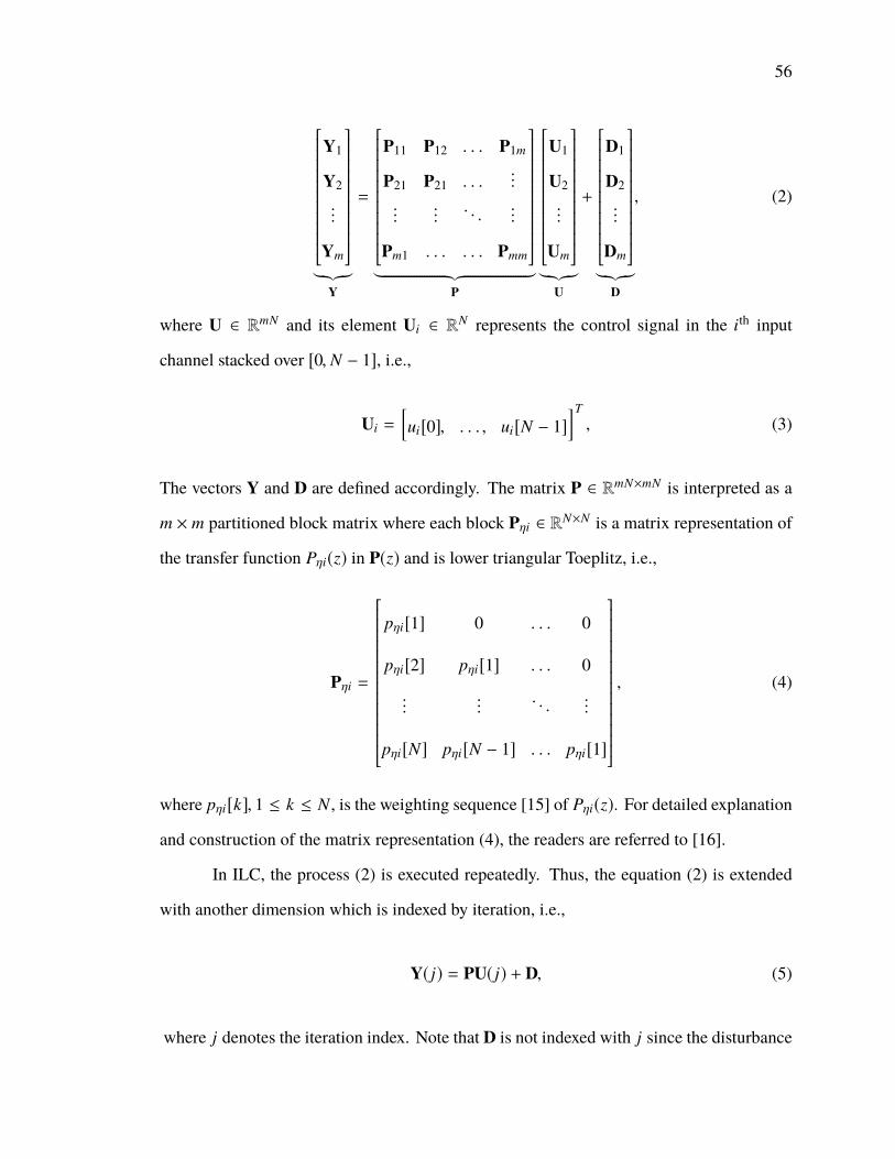
56

Y1

Y2...

Ym

︸︷︷︸Y

=

P11 P12 . . . P1m

P21 P21 . . ....

......

. . ....

Pm1 . . . . . . Pmm

︸ ︷︷ ︸P

U1

U2...

Um

︸︷︷︸U

+

D1

D2...

Dm

︸︷︷︸D

, (2)

where U ∈ RmN and its element Ui ∈ RN represents the control signal in the ith input

channel stacked over [0, N − 1], i.e.,

Ui =[ui[0], . . . , ui[N − 1]

]T, (3)

The vectors Y and D are defined accordingly. The matrix P ∈ RmN×mN is interpreted as a

m × m partitioned block matrix where each block Pηi ∈ RN×N is a matrix representation of

the transfer function Pηi(z) in P(z) and is lower triangular Toeplitz, i.e.,

Pηi =

pηi[1] 0 . . . 0

pηi[2] pηi[1] . . . 0

......

. . ....

pηi[N] pηi[N − 1] . . . pηi[1]

, (4)

where pηi[k], 1 ≤ k ≤ N , is the weighting sequence [15] of Pηi(z). For detailed explanation

and construction of the matrix representation (4), the readers are referred to [16].

In ILC, the process (2) is executed repeatedly. Thus, the equation (2) is extended

with another dimension which is indexed by iteration, i.e.,

Y( j) = PU( j) + D, (5)

where j denotes the iteration index. Note that D is not indexed with j since the disturbance

57

signal is assumed invariant in every iteration. Accordingly, the tracking error E in the j th

iteration is

E( j) = −PU( j) + E, (6)

where E = Yd −D, and Yd denotes the desired trajectory yd[k] in lifted system over length

[1, N]. Similar as in (2), the error E is expressed as

E =[ET

1, ET2, · · · , ET

m

]T, (7)

where ETi denotes the tracking error in the ith output channel in lifted system. The purpose

of ILC is to iteratively update the control input such that the output is as close as possible

to the desired trajectory. A widely used ILC update equation [7, 17] is

U( j + 1) = U( j) + LE( j), (8)

where L ∈ RmN×mN is the learning matrix for the entire multivariable system and is also

interpreted as a m × m partitioned block matrix

L =

L11 L12 . . . L1m

L21 L21 . . ....

......

. . ....

Lm1 . . . . . . Lmm

, (9)

in which each submatrix Lηi is responsible for learning the ηth output channel and updating

the control in the ith input channel. The resulting closed-loop iteration-domain error

dynamics is obtained combining the equations (6) and (8),

E( j + 1) = (I − PL)E( j). (10)

58

As an iterative algorithm, convergence of the ILC update equation (8) is important. Two

convergence definitions are discussed in the literature, i.e., convergence and zero-error

convergence [18].

Definition 1. (Convergence) A multivariable system (10) controlled with ILC is said to be

convergent if there exists a constant vector U∞ such that

limj→∞‖U( j) − U∞‖ = 0. (11)

Definition 2. (Zero-error Convergence) A multivariable system (10) controlled with ILC

(8) is said to be zero-error convergent if it is convergent, and further,

limj→∞‖E( j)‖ = 0. (12)

It is straightforward to conclude that convergence is less strict than zero-error con-

vergence. Satisfaction of the latter one implies that of the former one, but not otherwise.

The necessary and sufficient conditions for both definitions are stated in Theorems 1 and 2,

respectively.

Theorem 1. (Zero-error Convergence) A multivariable system (10) controlled with ILC (8)

is zero-error convergent if and only if [18]

ρ(I − PL) < 1, (13)

where for an arbitrary square matrix A, ρ(A) is the spectral radius of A.

Proof. Proof of this theorem directly follows asymptotic stability analysis for LTI systems

and can be found in [18].

59

Theorem 2. (Convergence) Denote r the rank of the matrix L, i.e., rank(L) = r . A multi-

variable system (10) controlled with ILC (8) is convergent if and only if all the eigenvalues

of the matrix I − PL are either inside or on the unit circle, i.e.,

|λi(I − PL)| ≤ 1, ∀1 ≤ i ≤ mN, (14)

where λi(A) refers to the ith eigenvalue of the matrix A, and the number of those on the unit

circle is mN − r , where mN is defined previously as the dimension of P and L.

Proof. Denote J the Jordan form of the matrix I − PL. It is well known that there exists a

similarity transformation matrix T such that

T−1(I − PL)T = J. (15)

Rewrite the equation (15),

L = P−1T(I − J)T−1. (16)

Combining equations (8) and (6) results in

∆U( j) = L(I − PL) jE(0), (17)

where ∆U( j) = U( j + 1) − U( j). It follows by substituting equations (15) and (16) into the

equation (17) that

∆U( j) = P−1T(I − J)J jT−1E(0). (18)

Sufficiency proof. Suppose the inequality (14) holds and there are mN − r eigenval-

ues on the unit circle. Since rank(P) = mN and rank(L) = r , then rank(PL) = mN − r .

Therefore, all eigenvalues of I − PL that are on the unit circle are exactly equal to one which

has multiplicity mN − r . Further, it is straightforward that the dimension of the eigenspace

corresponding to λ(I − PL) = 1 is also mN − r . Consequently, the Jordan form of I − PL

60

can be interpreted as

J =

J<1 0

0 I

, (19)

in which J<1 denotes the Jordan form containing the eigenvalues that are inside the unit

circle. Therefore,

limj→∞

J j =

0 0

0 I

, I − J =

I − J<1 0

0 0

. (20)

Note in the equation (17) that E(0) is finite. It follows that

limj→∞‖∆U( j)‖ = 0. (21)

The equation (21) implies that the sequence U( j)∞j=0 is Cauchy. Note that every finite

dimensional normed space is complete, and, thus, every Cauchy sequence in a finite di-

mensional normed space is convergent [19]. Since the vector U has finite dimension mN , it

follows that the sequence U j∞j=0 is convergent, i.e., there exists a constant vector U∞ such

that the equation (11) holds. This estabilishes the sufficiency of Theorem 2.

Necessity proof. The necessity of Theorem 2 is now proved. Suppose the sequence

U( j)∞j=0 is convergent. Since the normed space consisting of mN dimensional vectors and

the Euclidean norm is complete, it follows that the sequence U( j)∞j=0 is Cauchy, and, thus,

the equation (21) holds, which implies that the right hand of the equation (18) converges to

zero as j increases to infinity. Since the matrices P and T are in full rank, it follows that

limj→∞(I − J)J j = 0. (22)

61

The equation (22) indicates that the non-unity eigenvalues of J are strictly within the unit

circle and the unity eigenvalues are exactly at one. Further, the multiplicity of those equal

to one is the same as the the dimension the eigenspace corresponding to eigenvalue at

one. Since the matrices J and I − PL have the same eigenvalues and eigenspaces and

rank(PL) = r , it follows that all unity eigenvalues of I = PL are at one the multiplicity of

which is mN − r . This establishes the neccesity of Theorem 2.

2.2. NONZERO-ERROR CONVERGENCE PROBLEM FOR A SPECIAL CLASSOF MULTIVARIABLE SYSTEMS

Multivariable systems may have limited access to its output channels. For instance,

calibration of multiple industrial robots using one external metrology system can measure

only one robot at any time. Let S be a selection matrix and S ∈ S andS = S1, S2, · · · , Sm.

Each Si ∈ RmN×mN is interpreted as a block diagonal matrix which has m block diagonal

entries and each entry has dimension N × N . The ith diagonal entry is an identity matrix

whereas the other diagonal entries are zero, i.e.,

Si = blkdiag(0, · · · , 0, I, 0, · · · , 0)︸ ︷︷ ︸ith block is I

. (23)

The selection matrix S determines which output channel is currently available and thus used

for learning by pre-multiplying the error vector by S, i.e. SE. Consequently, the ILC update

equation for such systems and the resulting closed-loop error dynamics are

U( j + 1) = U( j) + LSE( j), (24)

E( j + 1) = (I − PLS)E( j). (25)

Note that although the learning matrix L is not changed, the effective learning matrix is

62

essentially LS due to the incomplete measurements. It is straightforward to conclude from

the equation (25) that such a system always violates the zero-error convergence condition

(13) since the error dynamics matrix I − PLS always has eigenvalues at one due to the

singularity of the matrix S, which implies that

ρ(I − PLS) ≥ 1. (26)

Although zero-error convergence is not possible for the system (24) and (25), it is always

expected in tracking problems. In the next section, a switching algorithm is proposed with

which the selection matrix S is swept through its domain. Conditions are given under which

the zero-error convergence is achieved with the proposed switching algorithm.

3. ILC-BASED SWITCHING ALGORITHM

3.1. SWICHING ALGORITHM

An ILC-based switching algorithm is presented in this section. It is shown above

that zero-error convergence cannot be accomplished with the standard ILC algorithm (24)

for each individual S ∈ S, due to the unknown information of some of the output channels.

It is possible, however, to achieve zero-error convergence if S is swept through the entire

domain S. The SILC algorithm proposed in this section consists of four steps: 1) Execute

the standard ILC update equation (24) for some S ∈ S for certain number of iterations Niter .

2) Pick a different S from S and repeat step 1). 3). Repeat step 2 until all elements in S

have been selected once. 4). Repeat the step 1) through 3) indefinitely. The details of the

proposed SILC algorithm are shown in Algorithm 1.

In Algorithm 1, the variables l and Nsw represent the current switch and the total

number of switches. The function mod(l,m) returns the remainder after division of l by m.

Consequently, by assigning Si to S, S sweeps through the entire domainS. The dynamics of

63

SILC algorithm has two dimensions, one in the iteration domain and the other in the switch

domain, i.e., when S is switched from one element to another element in S. Therefore, the

zero-error convergence conditions need be discussed in both domains, which are present in

the next two sections.

Algorithm 1: SILC Algorithm

1 Initialization: j = 0,U( j) = 0 ;

2 Y( j) = PU( j) + D ;

3 E( j) = R − Y( j) ;

4 for l ← 1 to Nsw do

5 i = f (l) where f (l) = mod(l,m) ;

6 if i == 0 then

7 i = m;

8 end

9 S = Si ;

10 for j ← 0 to Niter − 1 do

11 U( j + 1) = U( j) + LSE( j) ;

12 E( j + 1) = (I − PLS)E( j) ;

13 end

14 U(0) = U(Niter), E(0) = E(Niter);

15 end

3.2. ITERATION DOMAIN CONVERGENCE

Note from Algorithm 1 that the total number of iterations in each switch is Niter .

Given an initial error E(0) = E0 and a selection matrix S = Si, the tracking error after the

final iteration is complete is

64

E(Niter) = HiE0, (27)

where

Hi = (I − PLSi)Niter . (28)

In practice Niter is finite. The matrix Hi is, therefore, finite, and, thus E(Niter) is finite. In

an ideal situation, Niter is infinite, and, thus, E(Niter) can be unbounded. The following

theorem gives the condition under which E(Niter) is convergent as Niter →∞.

Theorem 3. The multivariable ILC system (24) and (25) is convergent for each i if and only

if

ρ(I − Pi·L·i) < 1, (29)

where Pi· and L·i respectively, are the ith block row of P and the ith block column of L, i.e.,

Pi· =[Pi1 Pi2 · · · Pim

],

L·i =[LT

1i LT2i · · · LT

mi

]T.

Proof. Consider first the case where S = S1. Then, rank(LS1) = (m − 1)N and

I − PLS1 =

I − P1·L·1 0 · · · · · · 0

−P2·L·1 I 0 · · · 0... 0 . . .

. . ....

......

. . .. . . 0

−Pm·L·1 0 · · · 0 I

. (30)

The matrix I − P1·L·1 is the only submatrix of I − PLS1 that contains the non-unity eigen-

values. Regarding LS1 as L and applying Theorem 2 establishes Theorem 3 for the case

of i = 1. The result is extended for all i by following a similar process. This establishes

Theorem 3.

65

Note that when S = Si, Niter → ∞, and Theorem 3 is satisfied, the matrix Hi has

closed form

Hi = limNiter→∞

(I − PLSi)Niter =

I · · · −P1·L·i(Pi·L·i)−1 · · · 0

.... . .

... · · ·...

0 · · · 0 · · · 0

......

.... . .

...

0 · · · −Pm·L·i(Pi·L·i)−1 · · · I

. (31)

We will use the equations (28) and (31) to express finite-iteration and convergent infinite-

iteration tracking error for the multivariable ILC system (24) and (25).

3.3. SWITCH DOMAIN CONVERGENCE

The remaining condition for SILC zero error convergence is referred to as switch-

domain convergence. We introduce some new notations here to facilitate the presentation

and the proof of the proposed conditions. Note from Algorithm 1 that there are the same set

of notations for controls U( j) and errors E( j) defined for every switch l. The values of these

notations in one switch may differ from that in another switch although the same notations

are used. To avoid this confusion, we augment U( j) and E( j) respectively to U( j, l) and

E( j, l) such that they are indexed by both iteration index j and the switch number l. The

algorithm using the modified notations is shown in Algorithm 2.

It is straightforward that from Algorithm 2 the final iteration of the switch l is used

as the initial iteration of the switch l + 1. Let U(l) and E(l) denote the control input and the

tracking error at the end of the lth switch, i.e.,

U(l) = U(Niter, l), E(l) = E(Niter, l). (32)

66

Then the error evolution from the end of the lth switch toward the end of the (l + 1)th switch

is

E(l + 1) = Hi= f (l+1)E(l), (33)

where the function f (l) is defined in Algorithm 1. The equation (33) describes the error

dynamics in the switch domain and is further expressed as

E(l) =( 1∏η=l

Hi= f (η)

)E0, (34)

where E0 is defined above as the initial error when learning is not enabled, and Hi is defined

in equation (28) for finite-iteration case and in equation (31) for infinite-iteration case. The

switch-domain convergence condition is stated in Theorem 4.

Algorithm 2: SILC Algorithm using the modified notations

1 Initialization: j = 0, l = 0,U( j, l) = 0 ;

2 Y( j, l) = PU( j, l) + D ;

3 E( j, l) = R − Y( j, l) ;

4 for l ← 1 to Nsw do

5 S = S f (l) ;

6 for j ← 0 to Niter − 1 do

7 U( j + 1, l) = U( j, l) + LSE( j, l) ;

8 E( j + 1, l) = (I − PLS)E( j, l) ;

9 end

10 end

Theorem 4. For a multivariable ILC system (24) and (25), if it is further controlled with

the switching algorithm as in Algorithm 1 and the iterative domain covergence condition in

Theorem 3 is satisfied, then the tracking error E(l) converges asymptotically to zero as the

67

switch number increases if

ρ( 1∏

i=m

Hi

)< 1. (35)

Proof. The proof of Theorem 4 follows [20] by viewing (33) as a linear periodically

time varying system and regarding the matrix product Hm · · ·H1 in (35) as a Monodromy

matrix.

3.4. SINGLE INPUT UPDATE SWITCHING ALGORITHM

For multivariable systems whose measurement access is limited to a single output

channel and whose control input update is limited to a single input channel, the ILC update

equation and the resulting error dynamics respectively are

U( j + 1) = U( j) + SLSE( j), (36)

E( j + 1) = (I − PSLS)E( j). (37)

The associative switching algorithm and the switching algorithm using the modified nota-

tions are identical to Algorithm 1 and Algorithm 2, respectively, except for that the matrix

LS is replaced by the matrix SLS. The iterative domain convergence condition is given in

Theorem 5, and the switch domain convergence condition is the same as that in Theorem

4, except for that the Hi matrix is different, which is given in Theorem 5 as well.

Theorem 5. The multivariable ILC system (36) and (37) is convergent for each i if and only

if

ρ(I − PiiLii) < 1, (38)

where Pii and Lii respectively, are the ith block diagonal entries of P and L. Note that in the

case of finite-iteration learning, the matrix Hi which characterizes the final tracking error

is

Hi = (I − PSLS)Niter, (39)

68

and in the case of infinite-iteration learning,

Hi =

I · · · −P11Lii(PiiLii)−1 · · · 0

.... . .

... · · ·...

0 · · · 0 · · · 0

......

.... . .

...

0 · · · −PmiLii(PiiLii)−1 · · · I

. (40)

Proof. The proof of Theorem 5 is similar to that of Theorem 3. The readers are suggested

to find the expression for the matrix I − PS1LS1, and then follow the same process as shown

in the proof of Theorem 3.

4. LEARNING MATRIX DESIGN FOR THE SWITCHING ALGORITHM

In order to accomplish zero-error convergence using the proposed ILC-based switch-

ing algorithm, two methods are introduced in this section to design an appropriate learning

matrix L, i.e., Plant Inversion design and Linearly Quadratic (LQ) optimization design,

such that both the iteration-domain convergence condition and the switch-domain conver-

gence condition are easily satisfied. Although the LQ optimization method is very popular

in standard ILC design, there are more restrictions on the weighting matrices, as will be

shown in this section, in the design of switching algorithm learning matrix than standard

ILC learning matrix.

4.1. PLANT INVERSION DESIGN

The plant inversion design is the most straightforward method to compute the

learning matrix L, which is obtained by directly inverting the nominal plant dynamics, i.e.,

69

L = P−1Λ, (41)

where P represents the nominal plant transfer matrix P(z) in lifted system structure, and

Λ = diag(Λ1, . . . ,Λm) is a block diagonal matrix. It is shown in [16] that both the

iteration-domain and the switch-domain convergence conditions of the SILC algorithm, i.e.,

Algorithm 1, hold provided that Λi ∈ RN×N satisfies ρ(I − Λi) < 1 and P = P. In particular

in the case that Λi = I and P = P, the deadbeat convergence is achieved, i.e., the tracking

error decreases to zero after all elements in S are selected once. Although in practice the

nominal dynamics and the actual dynamics never match due to the modeling uncertainties,

empirical studies have demonstrated that the plant-inversion design can tolerate modeling

uncertainties to some extent. The robustness discussion of the plant-inversion design with

the SILC algorithm is beyond the scope of this paper, and, thus, not discussed here.

4.2. LINEARLY QUADRATIC OPTIMIZATION DESIGN

For a standard ILC system (8) and (6), the LQ optimization for learning matrix

design is to minimize a cost function J [7], where

J(U( j + 1)) = ET ( j + 1)QET ( j + 1) + δUT ( j + 1)RδU( j + 1), (42)

in which δU( j + 1) = U( j + 1) − U( j) refers to the change in control input from the j th

iteration to the ( j + 1)th iteration, and Q and R are weighting matrices. For standard

ILC system, Q can be an arbitrary symmetric positive definite matrix and R can be any

symmetric semi-positive definite matrix, and the cost function (42) is minimized with the

constraint (8). The resulting learning matrix is

L = (PT QP + R)−1PT Q. (43)

70

The LT optimization is a generalization of the plant-inversion design. In other

words, the learning matrix in (41) is a sepcial case of the learning matrix in (43) by setting

Q R. The learning matrix L obtained in (43) does not necessarily guarantee zero-error

convergence if it is directly used in the switching algorithm, i.e., Algorithm 1. Indeed,

the resulting matrix L always satisfy the iteration-domain convergence condition (29) but

does not necessarily ensure the switch-domain convergence condition (35). In order to

resolve this issue, a more restrictive condition is imposed on the weighting matrices, i.e.,

the matrices Q and R need to to be diagonal matrices. These are formalized in Theorem 6.

Theorem 6. Suppose that the learning matrix L is obtained from the linearly quadratic

optimization design, i.e., the equation (43). If the multivariable ILC system (24) and (25)

is further controlled with the SILC algorithm, i.e., Algorithm 1, then the switch-domain

convergence condition (35) holds for both the finite-iteration learning and the infinite-

iteration learning, provided that the weighting matrices Q and R in (43) are of the form

Q = qI, R = rI,

where q > 0 and r ≥ 0.

Proof. This proof justifies the case where q r . It is straightforward to observe that

∀ε > 0, ∃q∗ > 0 such that

‖I − PL‖2 <ε√

N, ∀q ≥ q∗. (44)

Denote with coli(I − PL) the ith column matrix, i.e., the ((i − 1)N)th to (iN)th columns, of

the matrix I − PL. Following the Proposition 9.4.6 in [21], then,

‖coli(I − PL)‖2 ≤ ‖I − PL‖2 . (45)

71

Note that ∀F ∈ Rα×β, ‖F‖1 ≤ 1√β‖F‖2, and that coli(I − PL) = coli(I − PLSi). It follows

that

‖coli(I − PLSi)‖1 < ε. (46)

Observe from the equation (30) that the only nonzero elements in I − PLSi except for

coli(I − PLSi) are ones on its diagonal. Therefore,

‖I − PLSi‖1 = maxε, 1. (47)

Choose ε ≤ 1, then ‖I − PLSi‖1 = 1. With the equation (28), it follows that

‖Hi‖1 ≤ ‖I − PLSi‖Niter

1 ≤ 1, ∀Niter > 0. (48)

With the Corollary 9.4.5 in [21], it follows that

ρ( 1∏

i=m

Hi

)≤

( 1∏i=m

Hi

) 1

≤

1∏i=m

‖Hi‖1 ≤ 1. (49)

The remaining is to show that the second inequality in (49) is strict for matrices in the

structure of Hi, and thus Theorem 4 applies. To start with, it is assumed that m = 2 and

N = 1, and, thus

H1 =

(1 − P1·L·1)Niter 0

a 1

,H2 =

1 b

0 (1 − P1·L·1)Niter

(50)

where

a = −P2·L·1Niter−1∑

k=0(1 − P1·L·1)k, b = −P1·L·2

Niter−1∑k=0(1 − P2·L·2)k . (51)

In the case that Niter →∞, the matrices Hi in (50) have the same structure as in (31). Now

the problem is to prove

72

‖H2H1‖1 < ‖H2‖1 ‖H2‖1 , (52)

which, by the definition of ‖·‖1, implies that ∀z ∈ R2

max‖z‖1=1

‖H2H1z‖1 < ‖H2‖1 ‖H2‖1 . (53)

Note that ∀x, y ∈ R2 with ‖x‖1 = 1 and ‖y‖1 = 1,

‖H1x‖1 ≤ ‖H1‖1 , ‖H2y‖1 ≤ ‖H2‖1 , (54)

in which the equalities hold if and only if x = [0, 1]T and y = [1, 0]T . Suppose in the

contrary that ∃z∗, ‖z∗‖1 = 1 such that

‖H2H1z∗‖1 = ‖H2‖1 ‖H2‖1 . (55)

Then z∗ should satisfy the conditions that

z∗ = [0, 1]T, H1z∗ = [1, 0]T . (56)

However, it is obvious that the two conditions in (56) contradict with each other. Therefore,

the proposition that the inequality (53) is strict and consequently the inequality (52) is strict

is established. It is straightforward to extend this proposition to the case where m > 2

and N > 2. Therefore, the second inequality in (49) is strict, and, thus, Theorem 6 is

established.

Remark 1. Although it requires q r , and, thus, constraining the norm of the matrix

I − PL to a narrow area around the origin, the proof above provides strong mathematical

justification for Theorem 6. The advantage of this constraint is to provide high rate of con-

vergence. It, however, sacrifices the robustness of the algorithm to modeling uncertainties,

and, thus, may result in system divergence. In fact, the constraint (44) is not necessary.

73

Lemma 1 is proposed to justify Theorem 6 with the constraint (44) removed. The proof of

Lemma 1 is established for 2× 2 matrices. Its applicability to higher dimensional matrices,

although yet proved, are justified by running a large number of simulations.

Lemma 1. Let A ∈ Rn×n be a positive definite symmetric matrix. Let O = Ωigi=0 be a set

of diagonal matrix of dimension n × n, where the diagonal entries of each Ωi are either 0

or 1, and

g =

n∑k=0

(nk

)= 2n.

Let (α(1), α(2), . . . , α(n)) be an n − tuple such that α(i) ∈ 0, 1, 2, . . . , 2n ∀1 ≤ i ≤ n and

n∑i=1

Ωα(i) = I, (57)

where I denotes an identity matrix of dimension n × n. Then all eigenvalues of the matrix

product∏n

i=1(I − AΩα(i))κ are strictly inside the unit circle for all positive κ if all eigenvalues

of A are less than one, i.e.,

max

λ( n∏i=1(I − AΩα(i))

κ)

< 1 ∀κ > 0. (58)

Proof. The proof of Lemma 1 for the case of two by two matrices is shown in the Appendix.

The proof of Theorem 6 using Lemma 1 is also shown in the Appendix.

5. APPLICATION TOMULTI-AGENT COORDINATION

5.1. NOTATIONS USED IN MULTI-AGENT SYSTEMS

Consider a multi-agent system consisting of Na agents. The topology relation-

ship among the agents is typically described by a diagraph G = V, E,A, where

V = 1, 2, · · · , Na is the set of vertices which represent the corresponding agents, E

denotes the set of directed edges, and A = ai j ∈ RNa×Na is the weighting adjacency

74

matrix whose diagonal elements are zero and off-diagonal elements are non-negative, i.e.

aii = 0 and ai j ≥ 0 (i , j). A directed edge from the ith vertex to the j th vertex is

denoted by an ordered pair (i, j), representing that the j th agent could receive information

from the ith agent. The set E incorporates all effective edges. If a directed edge (i, j)

exists, then ai j = 1, otherwise, ai j = 0. For instance, the topology relationship of a three-

agent system shown in Figure 1 is described by G1 = V1, E1,A1, where V1 = 1, 2, 3,

E1 = (1, 2), (2, 3), (3, 1), and

A1 =

0 1 00 0 11 0 0

. (59)

Figure 1. Graphical representation of topology relationship of a three-agent system.

5.2. LINEAR MULTI-AGENT SYSTEMS AND CONSENSUS PROBLEM

For a multi-agent system whose topology is described by G, suppose that all agents

have the identical linear dynamics, i.e.,

xi[k + 1] = Fxi[k] +Gui[k]

yi[k] = Hxi[k], (60)

where xi, ui and yi respectively, represent the state, input, and output of the ith agent. The

75

multi-agent system (60) is said to achieve consensus if the states of all agents asymptotically

reach an agreement, i.e.,

limk→∞

x j[k] − xi[k] = 0, ∀i , j . (61)

A widely used consensus protocol in the literature is ui[k] = u f bi[k] where

u f bi[k] = KNa∑j=1

ai jwi j(x j[k] − xi[k]), (62)

where K is the feedback gain and W = wi j is a weighting matrix. A necessary and

sufficient condition [22] to achieve consensus (61) with the protocol (62) is that the diagraph

G incorporates a spanning tree [23], i.e., a subgraph which contains all vertices in G with

a minimum number of edges. Once this condition is satisfied, the parameters K and W are

tuned to achieve desired transient response. To get more insight on how these parameters

are determined, the readers are referred to [24].

5.3. RELATIVETRAJECTORYTRACKINGUSINGRELATIVE-INFORMATIONFEEDBACK CONTROL

While the consensus protocol (62) is targeted at achieving the agreement of the

states among all agents, it is extended to a generalized protocol with which every two

agents, provided an edge exists, maintain a desired dynamic relative trajectory. For the

agent i and the agent j, suppose the edge (i, j) ∈ E and a relative trajectory di j is desired

between them. Then the extended control protocol is

u f bi[k] = KNa∑j=1

ai jwi j(x j[k] − xi[k] − di j[k]). (63)

In the case a ji = 1, then

d ji[k] = −di j[k]. (64)

76

Note that if di j is a constant, then the relative state between the agent i and j asymptotically

arrives at a constant with the control protocol (63). A special case is di j = 0 ∀(i, j) ∈ E,

then the control protocol (63) is the same as the consensus protocol (62).

A unique feature of the control protocol (62) is that it only requires the relative

information to be available, e.g. relative position and relative velocity etc, which facilitates

the use of relative sensors where absolute sensor is not economic or has limited access. On

the other hand, since relative information is used alone, it only guarantees the asymptotic

relative trajectory tracking among agents, whereas there are infinite number of possible

global trajectories for each agent which depend on their initial conditions.

5.4. GLOBAL TRAJECTORY TRACKING COMBING FEEDBACK AND FEED-FORWARD CONTROL

Global trajectory tracking requires the global information of at least one agent to be

available. The measurement system possibly can access the global coordinate of only one

of the agents at any time. The control protocol (63) used in (60), however, has no control

on the global trajectories. In this section, we separate the control signal ui in (60) into two

parts, a feedback control signal u f bi and a feedforward control signal u f f i, i.e.,

ui[k] = u f bi[k] + u f f i[k]. (65)

The feedback control signalu f bi is generated by the control protocol (63) and the feedforward

control signal is generated by either the switching algorithm or the single input update

switching algorithm as proposed in the previous sections. Substitute the equation (65) in to

the equation (60) and concatenate the dynamics of all agents in a unified structure, we get

x[k + 1] = Fx[k] + drel[k]︸ ︷︷ ︸f eedback

+ Gu f f [k]︸ ︷︷ ︸f eedf orward

y[k] = Hx[k]

, (66)

77

where

x = [xT1, x

T2, · · · , x

TNa]T, u f f = [uT

1, uT2, · · · , u

TNa]T, y = [yT

1, yT2, · · · , y

TNa]T,

G = blkdiag(G,G, · · · ,G), H = blkdiag(H,H, · · · ,H),

and

drel =

−K∑Na

j=1 d1 j

−K∑Na

j=1 d2 j

...

−K∑Na

j=1 dNa j

F =

degin(1) Ka12w12 · · · Ka1Naw1Na

Ka21w21 degin(2) · · · Ka2Naw2Na

... . . .. . .

...

KaNa1wNa1 . . . . . . degin(Na)

, (67)

in which degin(i) = F−K∑Na

j=1 ai jwi jI and I is an identity matrix of the same dimension as

F. The function blkdiag(·) constructs block diagonal matrices for G and H, both of which

have Na block diagonal entries.

In the concatenated structure (66), the first two items on the right side of the first

equation is the closed-loop dynamics resulting from the feedback control (63), which is

responsible for relative trajectory tracking. In the case that dre f [k] = 0, the consensus

problem is resolved, i.e., the state of every agent converges to some indefinite vector. The

last item is responsible for global trajectory tracking of a particular agent. The introduction

of the switching algorithm and the single input update switching algorithm to designing

this item enables global trajectory tracking of all agents. To see how this works, the state

space equation (65) is transformed into the transfer function representation, i.e.,

y[k] = P(z)u f f [k] + d[k], (68)

where

P(z) = H(zI − F)−1G, d[k] = H(zI − F)−1drel[k] + H(zI − F)−1x[0].

78

Since the equation (68) is in the same structure as the equation (1), the SILC algorithm, the

single input update SILC algorithm, and the associated theories and design methods apply.

Remark 2. The conversion from the state space representation (66) to the transfer function

(68) assumes zero initial condition. The effect of nonzero initial condition on system

response is considered as a disturbance and represented by H(zI − F)−1x[0]. In this

work, it is assumed that the initial condition is invariant whenever the system is reset, and,

thus, resulting in repeated disturbance when the system is executed repeatedly. The SILC

algorithm and the single input update SILC algorithm, therefore, apply.

5.5. SIMULATION STUDY

Consider now anMAS system consiting of three agents whichmove in the horizontal

plane. The dynamics of the ith agent is described by

xi[k + 1] = xi[k] + ui[k]

yi[k] = xi[k], i = 1, 2, 3, (69)

where the state vector xi = [xi, yi]T denotes the position of the agent inCartesian coordinates.

The topology relationship of this system is described byG1 as defined previously. The initial

conditions of each agent respectively, are

x1[0] = [3.3, 3.4]T, x2[0] = [5.5, 0.5]T, x3[0] = [2.7, 0.7]T . (70)

Each agent is expected to follow its previous agent and move in a loop along the

triangle ABC as shown in Figure 2. The triangle is described by the vectors# »AB = [2,−2],

# »BC = [−2, 0], and# »CA = [0, 2]. The initial effective desired positions are described by

d12[1] = [−2,−2]T , d23[1] = [−2, 0]T , and d31[1] = [0, 2]T . The desired position starts at

k = 1 due to the one-step delay in system dynamics. Each agent is expected to spend equal

79

Figure 2. Illustration of desired relative trajectory and global trajectory for simulation study.

amount of time on all edges of the triangle, denoted byTp, and the overall time spent in a loop

is T f = 3Tp. The complete desired relative trajectories are then automatically determined.

Note that wherever the triangle is placed, the desired relative trajectories are not changed,

and, thus, relative trajectory tracking applies. If the triangle is restricted globally, then

the resulting desired trajectories are computed for each agent, and thus, global trajectory

tracking applies. In the simulation below for global trajectory tracking, the triangle is placed

at A = [1, 3], B = [3, 1], and C = [1, 1].

5.5.1. Relative Trajectory Tracking Using Feedback Control. Consider first the

case where the MAS system (69) is controlled only by the relative-information based

feedback controller (63). The feedback gainK = 0.08 is selected, and the weighting matrix

W adopted is

W =

1 0.4 0.6

0.5 1 0.5

0.8 0.2 1

. (71)

The simulation results are shown in Figure 3, where the desired relative trajectories and the

actual trajectories of each agent are depicted. Two observations are made from Figure 3.

First, although large tracking errors are observed, each agent roughly tracks its preceding

agent along the triangle. Second, the actual trajectories are far from the reference global

80

trajectories. These observations demonstrate that the feedback controller (63) achieves

relative-trajectory tracking, but fail to achieve global-trajectory tracking since no global

measurements are used in control.

Figure 3. Relative trajectory tracking using relative-information feedback control.

5.5.2. Global Trajectory Tracking Using SILC. Now we require the the MAS

system (69) to achieve global trajectory tracking as shown in Figure 3. In order to accomplish

this goal, the control ui is modified to incorporate a feedforward control signal, i.e., (65) is

used. A transfer function matrix P(z) is obtained by following the process in the Section

5.4, and the resulting system has six inputs and six outputs. Note that each agent has

two outputs, both of which are measured whenever an agent is accessed. Therefore, the

resulting six-input six-output system is regarded as a virtual three-input three-output system

by grouping the two output channels of each agent. The plant-inversion design method

with Λ = I is then adopted to obtain the learning matrix L for this three-input three-output

system.

The simulation results for the first three switches of learning are shown in Figure 4.

Figure 4 demonstrates that after three switches of learning, every agent succeeds in tracking

their global reference trajectories, a deadbeat control is achieved. It is also observed,

upon the completion of the first switch, that while agent 1 succeeds in tracking its global

reference trajectory, the other two agents behave as if only the original feedback controller

81

(a) First switch. (b) Second switch.

(c) Third switch.

Figure 4. Actual trajectories of each agent for the first three switches when SILC algorithmis applied.

functioned as in Figure 3. Similar observation is found for the second switch. This is

because the feedforward control signal obtained via the switching algorithm for the non-

globally-measured agent counteract the feedback control signals which would have driven

them to follow their precedent agents.

5.5.3. Global Trajectory Tracking Using Single Input Update SILC. To resolve

this issue, the single input update switching algorithm is utilized to generate the feedforward

control signal u f f i. In other words, the control signal obtained from the switching algo-

rithm is updated only for the globally-measured agent. Consequently, along each switch,

the associated globally-measured agent is expected to track its global reference with the

82

Figure 5. Actual trajectories of each agent for the 1st, 2nd, 3rd, 13th, 19th and the 30th switchwhen the single input update SILC algorithm is applied.

83

feedforward control, whereas the other agents are expected to maintain relative distances

with respect to their precedent agents with the closed-loop dynamics as in (66). The system

outputs, i.e., trajectories of each agent, after 1, 2, 3, 13, 19 and 30 switches of learning

respectively, are depicted in Figure 5. As shown in Figure 5, upon the completion of the

first switch, where the global information of the agent 1 is acquired, the agent 1 succeeds

in tracking its global reference while agent 2 and agent 3 are trying to follow agent 1 along

the triangle. Although large tracking errors are observed, similar observations are obtained

for the other switches. Further, it is also demonstrated from Figure 5 that as the number

of switches increases, for instance, upon the completion of the 30th switch, all agents tend

to perfectly track their global reference trajectories. This can also be seen from Figure 6,

where the tracking errors of each agent are depicted in the switch domain, measured in L-2

norm

Figure 6. Error evolution in the swich domain when single input update SILC applies.

6. SUMMARY AND CONCLUSIONS

Multivariable systems may have limited measurement access to their output chan-

nels, such as a multi-robot system equipped with one Laser Tracker. Zero error convergence

is not guaranteed when these systems are controlled with ILC, due to the singularity of the

84

effective learning matrix. In order to achieve zero convergent error, a switching algorithm

is proposed, with which the measurement device sweeps through all the output channels in

a predefined order, and ILC is executed for each accessed output channel. Two convergence

conditions need to be satisfied. The iteration-domain convergence condition ensures that

the error is always bounded while the switch-domain convergence condition guarantees that

the error asymptotically converges to zero. It has been shown that these two conditions

always hold for Linearly Quadratic (LQ) optimization design and plant-inversion design,

provided that Q = qI and R = rI where q, r > 0 in LQ design, and 0 < ρ(Λi) < 1 in

plant-inversion design.

The proposed switching algorithm is finally applied to a multi-agent formation

control problem. A low-level feedback controller is adopted for relative-trajectory tracking

based on the relative information, whereas the high-level ILC-based switching algorithm

is used to generate a feedforward control signal utilizing the global information. The

simulation results demonstrate that the switching algorithm may not be directly used in this

application since the feedforward signal counteracts the feedback control signal for those

non-globally-measured agents. To resolve this issue, single update switching algorithm is

used with which the feedforward control signal is enabled only for the current globally-

measured agent. Simulation results demonstrate that the tracking error is significantly

reduced after 19 switches. The current work focuses on the convergence of the error.

Future work would study the monotonic convergence conditions and the robustness of the

designing methods.

APPENDIX

PROOF OF LEMMA 1 FOR TWO BY TWOMATRICES

Proof. Let the matrix A be a symmetric positive definite matrix with all eigenvalues less

than one. Then,

85

A =

a1 a3

a3 a2

.The matrix A has the following properties:

1. |ai | < 1

2. a1 > 0, a2 > 0, 0 < det(A) < 1.

Let B = (I − AΩ2)κ(I − AΩ1)

κ. By some manipulations, we get

B =

1 −a3

1−(1−a2)κ

a2

0 (1 − a2)κ

(1 − a1)

κ 0

−a31−(1−a1)

κ

a11

=

(1 − a1)

κ + a23(1−(1−a2)

κ )(1−(1−a1)κ )

a1a2−a3

1−(1−a2)κ

a2

−(1 − a2)κa3

1−(1−a1)κ

a1(1 − a2)

κ

. (72)

Denote λ1,2 the eigenvalues of B. The following results are then obtained:

λ1 + λ2 = (1 − a1)κ + (1 − a2)

κ + a23(1 − (1 − a2)

κ)(1 − (1 − a1)κ)

a1a2, (73)

λ1λ2 = (1 − a1)κ(1 − a2)

κ . (74)

Since 0 < (1 − a1) < 1 and 0 < (1 − a2) < 1, the equations (73) and (74) indicate that

λ1,2 > 0. Suppose κ = 1. Solving the equations (73) and (74) for λ1,2, we get

λ1,2 =2 − a1 − a2 + a2

3 ±√(a1 + a2 − a2

3)2 + 4(a2

3 − a1a2)

2. (75)

Note from the property det(A) > 0 that a23 − a1a2 < 0. It follows that λ1,2 < 1. Suppose

κ = ∞. Solving the equations (73) and (74) for λ1,2, we get

86

λ1,2 = 0,a2

3a1a2, (76)

which implies λ1,2 < 1. Note that both λ1 + λ2 and λ1λ2 monotonically decrease as κ

increases. While the monotonic decrease of λ1λ2 is straightforward, that of λ1 + λ2 can be

seen by rewritting the right side of the equation (73), i.e.

λ1 + λ2 =(a1a2 − a2

3)((1 − a1)κ + (1 − a2)

κ) + a23(1 + ((1 − a1)

κ(1 − a2)κ)

a1a2. (77)

Also note that λ1 and λ2 are the roots of a quadratic polynomial, i.e. characteristic polyno-

mial ofB. Therefore, λ1+λ22 represents the line of symmetry of the characteristic polynomial.

The monotonic decrease of λ1 + λ2 implies that the graph of the characteristic polynomial

moves toward the negative direction of the horizontal axis. It can also be examined that

the span of the characteristic polynomial over the horizontal axis is monotonic decreasing.

Therefore, λ1 and λ2 always move toward to the negative direction, and approach infinites-

imally to the values obtained in (76) as κ → ∞. Consequently, 1 < λ1,2 < 1, ∀1 ≤ κ < ∞.

This establishes Lemma 1 for the case of two by two matrices.

PROOF OF THEOREM 6 USING LEMMA 1

Proof. Substitute Q = qI, R = rI into the equation (43) and premultiply L by P, we get

PL = qP(qPT P + rI)−1PT . (78)

Note that PL is symmetric positive definite and all its eigenvalues are less than one [25].

Further, not that the set S = Simi=1 ∈ O and that

∑mi=1 Si = I. Applying Lemma 1 results

in

max

λ( n∏i=1(I − PLSi)

κ)

< 1 ∀κ > 0, (79)

which indicates the switch-domain convergence condition (35) is satisfied.

87

REFERENCES

[1] Mikael Norrlof. “An adaptive iterative learning control algorithm with experimentson an industrial robot.” In: IEEE Transactions on robotics and automation 18.2(2002), pp. 245–251.

[2] Wenjie Chen and Masayoshi Tomizuka. “Dual-stage iterative learning control formimo mismatched system with application to robots with joint elasticity.” In: IEEETransactions on control systems technology 22.4 (2014), pp. 1350–1361.

[3] Douglas A Bristow and A-G Alleyne. “A high precision motion control system withapplication to microscale robotic deposition.” In: IEEE Transactions on ControlSystems Technology 14.6 (2006), pp. 1008–1020.

[4] Kira L Barton and Andrew G Alleyne. “A cross-coupled iterative learning controldesign for precision motion control.” In: IEEE Transactions on Control SystemsTechnology 16.6 (2008), pp. 1218–1231.

[5] Tom Oomen et al. “Connecting system identification and robust control for next-generationmotion control of awafer stage.” In: IEEETransactions onControl SystemsTechnology 22.1 (2014), pp. 102–118.

[6] Angela P Schoellig, Fabian L Mueller, and Raffaello D’Andrea. “Optimization-based iterative learning for precise quadrocopter trajectory tracking.” In:AutonomousRobots 33.1-2 (2012), pp. 103–127.

[7] Douglas A Bristow, Marina Tharayil, and Andrew G Alleyne. “A survey of iterativelearning control.” In: IEEE Control Systems 26.3 (2006), pp. 96–114.

[8] Tucker Balch and Ronald C Arkin. “Behavior-based formation control for multirobotteams.” In: IEEE transactions on robotics and automation 14.6 (1998), pp. 926–939.

[9] Nathan Michael, Jonathan Fink, and Vijay Kumar. “Cooperative manipulation andtransportation with aerial robots.” In: Autonomous Robots 30.1 (2011), pp. 73–86.

[10] Andreas Hock and Angela P Schoellig. “Distributed iterative learning control for ateam of quadrotors.” In: Decision and Control (CDC), 2016 IEEE 55th Conferenceon. IEEE. 2016, pp. 4640–4646.

[11] Zhijun Li et al. “Decentralized fuzzy control of multiple cooperating robotic manip-ulators with impedance interaction.” In: IEEE Transactions on Fuzzy Systems 23.4(2015), pp. 1044–1056.

[12] Deyuan Meng and Yingmin Jia. “Iterative learning approaches to design finite-timeconsensus protocols for multi-agent systems.” In: Systems & Control Letters 61.1(2012), pp. 187–194.

88

[13] Hyo-Sung Ahn and YangQuan Chen. “Iterative learning control for multi-agent for-mation.” In: ICCAS-SICE, 2009. IEEE. 2009, pp. 3111–3116.

[14] He Li, Douglas A Bristow, and Robert G Landers. “A switched estimation strategybased on Kalman filtering for compensating laser tracker ADM shift.” In: PrecisionEngineering (2019).

[15] Katsuhiko Ogata. Discrete-time control systems. Vol. 2. Prentice Hall EnglewoodCliffs, NJ, 1995.

[16] He Li, Douglas A Bristow, and Robert G Landers. “A plant-inversion based switchediterative learning control scheme for a special class of multivariable systems.” In:ASME 2018 Dynamic Systems and Control Conference. to appear. Sept. 2018.

[17] RichardWLongman. “Iterative learning control and repetitive control for engineeringpractice.” In: International journal of control 73.10 (2000), pp. 930–954.

[18] Mikael Norrlöf and Svante Gunnarsson. “Time and frequency domain convergenceproperties in iterative learning control.” In: International Journal of Control 75.14(2002), pp. 1114–1126.

[19] Erwin Kreyszig. Introductory functional analysis with applications. Vol. 1. wileyNew York, 1978.

[20] Norman M Wereley. “Analysis and control of linear periodically time varying sys-tems.” PhD thesis. Massachusetts Institute of Technology, 1990.

[21] Dennis S Bernstein. Matrix mathematics: Theory, facts, and formulas with applica-tion to linear systems theory. Vol. 41. Princeton university press Princeton, 2005.

[22] Wei Ren, Randal W Beard, and Ella M Atkins. “A survey of consensus problems inmulti-agent coordination.” In: American Control Conference, 2005. Proceedings ofthe 2005. IEEE. 2005, pp. 1859–1864.

[23] tutorialspoint. Data Structures and Algorithms - Spanning Tree. url: https://www.tutorialspoint.com/data_structures_algorithms/spanning_tree.htm.

[24] Ya Zhang and Yu-Ping Tian. “Consentability and protocol design of multi-agentsystems with stochastic switching topology.” In: Automatica 45.5 (2009), pp. 1195–1201.

[25] Notker Amann, David H Owens, and Eric Rogers. “Iterative learning control fordiscrete-time systems with exponential rate of convergence.” In: IEE Proceedings-Control Theory and Applications 143.2 (1996), pp. 217–224.

89

SECTION

4. SUMMARY AND CONCLUSIONS

This thesis studies controlled switching in the estimation of a temporal shift in a

Laser Tracker (LT), and in multivariable Iterative Learning Control (ILC) systems where

only partial outputs are measured at any time. It turns out that the introduction of the

controlled switching into the estimation process and the control system has increased

the flexibility of both to execute more complex tasks and to achieve better performance,

respectively.

To be specific, in Paper I, the estimation of the LT ADM shift is switched between

Kalman Filtering (KF) and model-based prediction . This enables the LT to execute two

conflicting tasks, i.e., shift measurement and normal operation, which could not have been

done if only one of KF or prediction is utilized. On the one hand, the more time spent on

shift measurement, the more accurate the resulting estimation. On the other hand, the more

time spent on normal operation, the more productive the overall process. The controlled

switching allows making a tradeoff between them and thus achieving desired performance.

Paper II has shown that zero tracking error cannot be achieved for multivariable ILC systems

where only partial outputs are measured at any time. In order to accomplish zero tracking

error, a controlled switching algorithm is developed with which the output channels are

measured in a sequential order, and the standard ILC is executed for each measured output.

It is proved that if all eigenvalues of the switch-domain error dynamics matrix are strictly

within the unit circle, then the tracking errors in all output channels converge to zero as the

switching continues.

90

Both Paper I and Paper II have demonstrated the promise of controlled switching

in enabling a system to achieve more complex tasks, which could not have been done if

the switching is disabled. However, improvements can be made in future. In Paper I, the

switching relies heavily on the accuracy of the system model. The switching algorithm may

be improved by making the switching decision based on the innovation term. In Paper II,

the convergence condition only guarantees zero error convergence. However, the transition

growth may become unrealistic. Therefore, future direction may focus on studying the

monotonic convergence conditions.

91

REFERENCES

[1] Daniel Liberzon. Switching in systems and control. Springer Science & BusinessMedia, 2003.

[2] He Li, Robert G Landers, and Douglas A Bristow. “Modeling of Absolute DistanceMeter Shift Inside a Laser Tracker.” In: ASME 2017 12th International Manufac-turing Science and Engineering Conference collocated with the JSME/ASME 20176th International Conference on Materials and Processing. American Society ofMechanical Engineers. 2017, V003T04A071–V003T04A071.

[3] He Li, Douglas A Bristow, and Robert G Landers. “A Switched Iterative LearningControl Scheme for Two-Input Two-Output Systems.” In: 2018 Annual AmericanControl Conference (ACC). IEEE. 2018, pp. 5600–5605.

[4] He Li, Douglas A Bristow, and Robert G Landers. “A plant-inversion based switchediterative learning control scheme for a special class of multivariable systems.” In:ASME 2018 Dynamic Systems and Control Conference. to appear. Sept. 2018.

[5] Rudolph Emil Kalman. “A new approach to linear filtering and prediction problems.”In: Journal of basic Engineering 82.1 (1960), pp. 35–45.

[6] Anastasios I Mourikis and Stergios I Roumeliotis. “A multi-state constraint Kalmanfilter for vision-aided inertial navigation.” In: Proceedings 2007 IEEE InternationalConference on Robotics and Automation. IEEE. 2007, pp. 3565–3572.

[7] Thomas Schuhmann, Wilfried Hofmann, and Ralf Werner. “Improving operationalperformance of active magnetic bearings using Kalman filter and state feedbackcontrol.” In: IEEE Transactions on Industrial Electronics 59.2 (2012), pp. 821–829.

[8] Xiaoping Yun and Eric R Bachmann. Design, implementation, and experimental re-sults of a quaternion-based Kalman filter for human body motion tracking. Tech. rep.NAVAL POSTGRADUATE SCHOOL MONTEREY CA DEPT OF ELECTRICALand COMPUTER . . ., 2006.

[9] Dong-Jun Lee and Masayoshi Tomizuka. “Multirate optimal state estimation withsensor fusion.” In: Proceedings of the 2003 American Control Conference, 2003.Vol. 4. IEEE. 2003, pp. 2887–2892.

[10] Simon J Julier and Jeffrey K Uhlmann. “New extension of the Kalman filter tononlinear systems.” In: Signal processing, sensor fusion, and target recognition VI.Vol. 3068. International Society for Optics and Photonics. 1997, pp. 182–194.

92

[11] Greg Welch, Gary Bishop, et al. “An introduction to the Kalman filter.” In: (1995).

[12] Eric A Wan and Rudolph Van Der Merwe. “The unscented Kalman filter for non-linear estimation.” In: Proceedings of the IEEE 2000 Adaptive Systems for SignalProcessing, Communications, and Control Symposium (Cat. No. 00EX373). Ieee.2000, pp. 153–158.

[13] Dan Simon.Optimal state estimation: Kalman, H infinity, and nonlinear approaches.John Wiley & Sons, 2006.

[14] Suguru Arimoto, Sadao Kawamura, and Fumio Miyazaki. “Bettering operation ofrobots by learning.” In: Journal of Robotic systems 1.2 (1984), pp. 123–140.

[15] Giuseppe Casalino and Giorgio Bartolini. “A learning procedure for the controlof movements of robotic manipulators.” In: IASTED symposium on robotics andautomation. Vol. 108. 1984.

[16] John JCraig. “Adaptive control ofmanipulators through repeated trials.” In:AmericanControl Conference. 21. 1984, pp. 1566–1573.

[17] Tom Oomen et al. “Connecting system identification and robust control for next-generationmotion control of awafer stage.” In: IEEETransactions onControl SystemsTechnology 22.1 (2014), pp. 102–118.

[18] JoostBolder et al. “Using iterative learning controlwith basis functions to compensatemedium deformation in a wide-format inkjet printer.” In:Mechatronics 24.8 (2014),pp. 944–953.

[19] Douglas A Bristow and A-G Alleyne. “A high precision motion control system withapplication to microscale robotic deposition.” In: IEEE Transactions on ControlSystems Technology 14.6 (2006), pp. 1008–1020.

[20] Brian E Helfrich et al. “Combined H − ∞-Feedback Control and Iterative LearningControl Design With Application to Nanopositioning Systems.” In: IEEE Transac-tions on Control Systems Technology 18.2 (2010), pp. 336–351.

[21] Patrick M Sammons, Douglas A Bristow, and Robert G Landers. “Iterative learningcontrol of bead morphology in laser metal deposition processes.” In: 2013 AmericanControl Conference. IEEE. 2013, pp. 5942–5947.

[22] Deyuan Meng and Yingmin Jia. “Iterative learning approaches to design finite-timeconsensus protocols for multi-agent systems.” In: Systems & Control Letters 61.1(2012), pp. 187–194.

[23] Andreas Hock and Angela P Schoellig. “Distributed iterative learning control for ateam of quadrotors.” In: Decision and Control (CDC), 2016 IEEE 55th Conferenceon. IEEE. 2016, pp. 4640–4646.

93

[24] Douglas A Bristow, Marina Tharayil, and Andrew G Alleyne. “A survey of iterativelearning control.” In: IEEE Control Systems 26.3 (2006), pp. 96–114.

[25] RichardWLongman. “Iterative learning control and repetitive control for engineeringpractice.” In: International journal of control 73.10 (2000), pp. 930–954.

[26] Katsuhiko Ogata. Discrete-time control systems. Vol. 2. Prentice Hall EnglewoodCliffs, NJ, 1995.

[27] Chi-Tsong Chen. Linear system theory and design. Oxford University Press, Inc.,1998.

[28] Douglas A Bristow et al. “High bandwidth control of precision motion instrumenta-tion.” In: Review of Scientific Instruments 79.10 (2008), p. 103704.

[29] Mikael Norrlöf and Svante Gunnarsson. “Time and frequency domain convergenceproperties in iterative learning control.” In: International Journal of Control 75.14(2002), pp. 1114–1126.

[30] Douglas A Bristow and John R Singler. “Towards transient growth analysis anddesign in iterative learning control.” In: International Journal of Control 84.7 (2011),pp. 1234–1245.

[31] Jurgen van Zundert and Tom Oomen. “On inversion-based approaches for feedfor-ward and ILC.” In: Mechatronics 50 (2018), pp. 282–291.

[32] K Mike Tao, Robert L Kosut, and Gurcan Aral. “Learning feedforward control.” In:Proceedings of 1994 American Control Conference-ACC’94. Vol. 3. IEEE. 1994,pp. 2575–2579.

[33] Jay H Lee, Kwang S Lee, and Won C Kim. “Model-based iterative learning controlwith a quadratic criterion for time-varying linear systems.” In: Automatica 36.5(2000), pp. 641–657.

[34] Notker Amann, David H Owens, and Eric Rogers. “Iterative learning control fordiscrete-time systems with exponential rate of convergence.” In: IEE Proceedings-Control Theory and Applications 143.2 (1996), pp. 217–224.

94

VITA

He Li was born in Jinan, Shandong, China. He received his Bachelor’s degree in

Mechanical Engineering and Automation from Shandong University of Technology, China

in June 2015 and joined Missouri University of Science and Technology in May 2016. He

worked as Graduate Research Assistant in the Precision Motion Control Lab advised by Dr.

Douglas A. Bristow and co-advised by Dr. Robert G. Landers. He received his Master of

Science in Mechanical Engineering in July 2019 from Missouri University of Science and

Technology. His research was in robotics, iterative learning control, and Kalman filtering.

He published four conference papers and two journal papers.