IOP PUBLISHING INVERSE PROBLEMS

Inverse Problems 25 (2009) 035006 (34pp) doi:10.1088/0266-5611/25/3/035006

An iterative representer-based scheme for datainversion in reservoir modeling

Marco A Iglesias and Clint Dawson

Center for Subsurface Modeling-C0200, Institute for Computational Engineering and Sciences(ICES), The University of Texas at Austin, Austin, TX 78712, USA

E-mail: iglesias@ices.utexas.edu

Received 30 November 2008Published 15 January 2009Online at stacks.iop.org/IP/25/035006

Abstract

In this paper, we develop a mathematical framework for data inversion inreservoir models. A general formulation is presented for the identificationof uncertain parameters in an abstract reservoir model described by a set ofnonlinear equations. Given a finite number of measurements of the state andprior knowledge of the uncertain parameters, an iterative representer-basedscheme (IRBS) is proposed to find improved parameters. In this approach, therepresenter method is used to solve a linear data assimilation problem at eachiteration of the algorithm. We apply the theory of iterative regularization toestablish conditions for which the IRBS will converge to a stable approximationof a solution to the parameter identification problem. These theoretical resultsare applied to the identification of the second-order coefficient of a forwardmodel described by a parabolic boundary value problem. Numerical resultsare presented to show the capabilities of the IRBS for the reconstruction ofhydraulic conductivity from the steady-state of groundwater flow, as wellas the absolute permeability in the single-phase Darcy flow through porousmedia.

(Some figures in this article are in colour only in the electronic version)

1. Introduction

The main challenge of reservoir management is to achieve the maximum hydrocarbon recoveryunder the minimum operational costs. This goal cannot be accomplished without a reservoirsimulator capable of predicting the reservoir performance. However, the reliability of reservoirmodels depends on the accuracy of the knowledge of the subsurface properties. Theseproperties are highly heterogeneous and can be measured at few locations. Therefore, in orderto obtain an accurate reservoir model, it is essential to develop techniques that allow us tocharacterize the petrophysical properties of the subsurface.

0266-5611/09/035006+34$30.00 © 2009 IOP Publishing Ltd Printed in the UK 1

Inverse Problems 25 (2009) 035006 M A Iglesias and C Dawson

Automatic history matching is one of the aspects involved in the characterization of thepetrophysical properties of a reservoir. The aim of history matching is to obtain estimatesof the petrophysical properties, so that the model prediction fits the observed productiondata. Traditionally, data acquisition for history matching was available by well-loggingtechniques which were expensive and required well intervention. However, after 1997 [15],the development of smart-well technology has dramatically changed the restrictive scenariofor data acquisition. With the aid of down-hole permanent sensors, it is possible to monitorproduction data in almost real time. These data may be used for history matching in order toobtain a better characterization of the reservoir which in turn can be used to optimize recovery.Unfortunately, classical history matching techniques are not able to process large sets of dataunder reasonable computational cost. For this reason, the reservoir community has startedto implement techniques that have been previously used in other areas. Such is the case inphysical oceanography and meteorology [6, 8, 13, 30, 34], where several data assimilationtechnologies have been developed to overcome analogous problems to those faced by thereservoir community.

Within the broad methods for data assimilation, we distinguish between two mainapproaches that have been applied to the reservoir modeling application: the Monte Carlo-type or probabilistic framework [12] and the variational approach [6]. The former consists ofgenerating an ensemble of different possible realizations of the state variable with given priordistribution. The model is run for each member of the ensemble up to the first measurementtime. Then, each state variable is updated with standard formulae of Kalman filteringtheory [22] to produce a posterior distribution which is used to continue the process. Inthe Kalman filter-type methods, the model simulator is used as a black box without theneed of an adjoint code. This feature offers a significative advantage in history matchingfor which several applications of the ensemble Kalman filter (EnKF) have been conducted[9, 14, 17, 18, 24–27, 31]. However, there are still open questions arising from the EnKFimplementation. Unphysical solutions, overestimation and poor uncertainty quantificationhave been reported with the EnKF [17, 18]. Despite attempts to remediate these undesiredoutcomes, the nonlinearity of reservoir models clearly goes beyond the capabilities of theEnKF.

In the variational approach, the solution is sought as a minimizer of a weighted least-squares functional that penalizes the misfit between model-based and real measurements.The corresponding minimization involves the implementation of an optimization techniquewhich typically requires the development of an adjoint code for the efficient computationof the derivatives of the cost functional. It is worth mentioning that many variationalapproaches for history matching have been studied during the last few years. However, thoseapproaches are suboptimal and computationally expensive because of the highly nonlinearand large-scale reservoir models. For this reason, variational ‘data assimilation’ techniqueshave received attention for reservoir and groundwater applications [2–4, 21, 29, 33]. Inlinear variational ‘data assimilation’, an inexpensive minimization of a weighted least-squarescost functional can be conducted by the so-called representer method [6]. Assuming thatthe measurement space is finite dimensional, the representer method provides the solutionto the Euler–Lagrange equations (E–L) resulting from the variational formulation. Fornonlinear problems, the representer method cannot be implemented directly. Nevertheless,some representer-based techniques have been explored to compute an approximation to thesolution of the E–L equations [3, 29]. However, these approaches do not necessarily yield adirection of descent of the cost functional. Therefore, an additional technique such as linesearch is needed to accelerate or even obtain convergence [3, 29, 33]. Unfortunately, theseadditional implementations may compromise the efficiency required for reservoir applications.

2

Inverse Problems 25 (2009) 035006 M A Iglesias and C Dawson

In this paper, we present a novel implementation of the representer method as an iterativeregularization scheme. The problem is posed in terms of a parameter identification problemwhere the objective is to find a parameter such that the model output fits the data within someerror. In this formulation, a solution (identified parameters) is the limit of a sequence ofsolutions to linearized inverse problems. Each of these inverse problems is the minimizationof a weighted least-squares functional that incorporates prior knowledge of the reservoir.In addition, we applied standard techniques from iterative regularization theory [10, 19] toobtain convergence results for the proposed scheme. Both analytical and numerical resultsshow that this methodology is efficient, robust and therefore promising for the estimation ofpetrophysical properties in reservoir models.

The robustness of the presented methodology is ensured by convergence results that werefirst developed by Hanke [19] in a more general framework. However, in our approach, weconsider an implicit system (see equation (2)) instead of the parameter-to-observation map of[19]. The reason for this selection comes from the fact that the reservoir model is commonlydescribed by a set of PDEs for which energy inequalities may be available. Second, we alwaysassume that the observation space is finite dimensional so that the representer method can beapplied. In contrast to [19], with the aforementioned property we do not need to interpolate thedata which always come as a finite-dimensional set. Third, in our formulation we incorporateprior knowledge which is relevant to the application. Despite some subtle differences betweenour methodology and the one presented in [19], we show that our approach is a particularcase of Hanke’s work in the case of a fixed Levenberg–Marquardt parameter α = 1 and anappropriate selection of the parameter norm.

The outline of the paper is the following. In section 2, with the aid of the standard theory ofparameter identification [10], we introduce an abstract formulation for parameter identificationin reservoir models. In section 2.6, an iterative representer-based scheme (IRBS) is proposedfor the computation of a solution to the parameter identification problem. Since it is assumedthat the observation space is finite dimensional, we apply the representer method that we derivein section 2.7. In section 2.8, we discuss the required hypotheses for convergence of the IRBS.In section 3, we study an application of the IRBS to the identification of the second-ordercoefficient in a parabolic boundary value problem. For this case, the implementation of theIRBS is discussed in section 3.1. Finally, in section 4 we show some numerical experimentsto determine the capability of the IRBS for the reconstruction of subsurface properties.

2. Data inversion in reservoir models

In order to illustrate our approach, we first present a model problem that will be used in thesubsequent sections for the validation of IRBS. We consider single-phase Darcy flow throughporous media which is described by the following equation [5]:

cφ∂p

∂t− 1

μ∇ · eY ∇p = f, (1)

where c is the compressibility of the fluid, φ is the porosity, μ is the viscosity of the fluidand f is an injection/production rate. K = eY is the absolute permeability and p is thepressure. When c, μ, φ,K are given and some initial and boundary conditions are prescribed,then (1) can be solved uniquely for p in the appropriate spaces [23]. In this model, φ and Kare the petrophysical properties associated with the reservoir. In practical applications, theseparameters are ‘uncertain’ in the sense that only prior knowledge is available. In general,this knowledge does not capture the characteristics required for an accurate description of thereservoir. Therefore, if those parameters were utilized in (1), the solution would be different

3

Inverse Problems 25 (2009) 035006 M A Iglesias and C Dawson

from the measurements collected at the wells. Then, we need to address the following inverseproblem. Given measurements collected at the well and prior knowledge of the petrophysicalproperties find improved parameters such that the model matches the measurements from thereservoir.

2.1. Preliminaries and notation

For any vector v ∈ RN we denote by ‖v‖ = (∑N

i=1 |vi |2)1/2

the Euclidian norm. ForA ∈ R

N×N we also denote by ‖A‖ = sup‖v‖�=0‖Av‖‖v‖ . For any symmetric positive-definite

matrix C ∈ RN×N , we denote by ‖v‖C = (vT Cv)1/2 the corresponding induced norm in

RN . Given a Hilbert space H, we denote the closed ball centered at k of radius r by B(r, k).

Furthermore, the inner product of H is denoted by 〈·, ·〉H. Given � ⊂ RN and 0 < T < ∞,

we define � = ∂�,�T = � × (0, T ) and �T = � × (0, T ). We consider [23] the usualSobolev spaces H 2(�) with the norm given by ‖u‖H 2(�) = (∑

|α|�2

∫�

‖Dαu‖2)1/2

, and

H 1(0, T ;L2(�)) with the norm ‖u‖H 1(0,T ;L2(�)) = (∫ T

0 ‖u(t)‖2L2(�)

dt)1/2

. Additionally,

we define the space H 2,1(�T ) = L2(0, T ;H 2(�)) ∩ H 1(0, T ;L2(�)) with the norm‖u‖H 2,1(�T ) = (∫ T

0 ‖u(t)‖2H 2(�)

dt + ‖u‖2H 1(0,T ;L2(�))

)1/2. Finally, we define H 1/2,1/4(�T ) =

L2(0, T ;H 1/2(�))∩H 1/4(0, T ;L2(�)) with the norm ‖u‖H 1/2,1/4(�T ) = (∫ T

0 ‖u(t)‖2H 1/2(�)

dt +

‖u‖2H 1/4(0,T ;L2(�))

)1/2where H 1/2(�) and H 1/4(0, T ;L2(�)) are interpolation spaces defined

in the sense of definition 2.1 in [23].

2.2. The forward model

The objective of this section is to develop a general mathematical framework for the estimationof uncertain parameters in a reservoir model described by an abstract nonlinear system inHilbert spaces. Let us represent the reservoir by an open bounded and convex set � ⊂ R

l

with l = 2, 3 with C1 boundary. Given some 0 < T < ∞, suppose that [0, T ] is the time ofinterest for the analysis of the reservoir dynamics. Assume that the reservoir has N uncertainparameters. The corresponding parameter space is defined by K = �N

i=1Ki where each Ki isa linear subspace either of L2(�) or L2(�T ). Let S and Z be arbitrary subspaces of L2(�T ).The set S is the space of all possible states of the reservoir. We now assume that the dynamicsof the reservoir can be described, over a finite interval of time [0, T ], by a set of (forward)model equations

G(k, s) = 0, (2)

where G : K × S → Z is a nonlinear operator. For a fixed parameter k ∈ K, an elementof the state space s(x, t) ∈ S that satisfies (2) is the corresponding state of the reservoirwhich simulates the reservoir dynamics over the interval of time. Parameters which are notconsidered uncertain in the sense described above are assumed to be contained in the functionalrelation chosen for the operator G. The subspaces S,K and Z , in addition to the functionalrelation for G, must be defined for the particular reservoir model of interest.

2.3. Measurements and prior knowledge

Each measurement is treated independently at each location and time of collection. Let ussuppose that we are given dη = [

dη

1 , . . . , dη

M

]a vector of M measurements of the state of the

reservoir, such that each dηm was collected at (xm, tm). In general, measurements are corrupted

4

Inverse Problems 25 (2009) 035006 M A Iglesias and C Dawson

by noise. In other words, the vector of measurements dη is only an approximation to themeasurements of the state, that is

‖dη − d‖C−1 � η, (3)

where d = [d1, . . . , dM ] is the vector of perfect (noise-free) measurements, and the normin (3) is weighted by the inverse of a positive-definite covariance matrix C. The observationprocess responsible for a perfect measurement dm is represented, on the space S, by the action(Lm(s) = dm) of a linear functional Lm : S → R. Furthermore, prior knowledge informationfor each uncertain parameter ki is required to be given as a prior mean ki and the correspondingprior error covariance function Cki

. In summary, the following information must be provided:

(D1) dη = [d

η

1 , . . . , dη

M

]a vector of M (possibly corrupted by noise) measurements of the state

of the reservoir at {(xm, tm)}Mm=1.(D2) Prior measurements (error) covariance matrix C (positive definite).(D3) Prior knowledge of parameters k = [k1, . . . , kN ].(D4) Parameters prior error covariance operators {Ck1, . . . , CkN

}.(D5) Expressions for the linear functionals L = [L1, . . . ,LM ] representing the process from

which dη = [d1, . . . , dM ] was obtained.

2.4. Fundamental definitions

Inspired by the standard theory of parameter identification [10, 19], we now formulate

Definition 2.1. Assume that the state of the system is described by (2) and the measurementprocess is represented by L = [L1, . . . ,LM ] as described above. Given a vector d =[d1, . . . , dM ] of exact measurements (noise free) of the state of the system, a solution to theparameter identification problem (PIP) is an element k ∈ K, such that

G(k, s) = 0, and L(s) = d (4)

for some s ∈ S.

Note from the previous definition that no assumption has been made on the uniqueness of thesolution to the PIP. Furthermore, as we indicated earlier, usually the vector of measurementsd is not available but only a noisy version dη given by (3). In this case, the computation of asolution to the PIP will be understood as a stable approximation in the limit η → 0.

Suppose for a moment that we are given a set of perfect (noise-free) measurements. Ifin addition we assume that the model dynamics and measurement process are representedcorrectly by the mathematical models under consideration, then, it is reasonable to think thatthe measurements were obtained from the ‘true state’ sT of the system which satisfies themodel dynamics (2) for some ‘true parameter’ kT . For this reason we postulate the following:

Attainability condition of data. There exists at least one solution kT ∈ K to the PIP. We referto kT as the ‘true parameter’.

For example, suppose we are interested in the identification of K in model (1) given pressuredata from some well locations (assuming that c, φ and μ are perfectly known). It is clear thatthere may be several permeability configurations that will generate the same pressure responsewhich is measured at the wells. However, the reservoir has one and only one permeabilityfield which is responsible for the generation of the collected measurements.

5

Inverse Problems 25 (2009) 035006 M A Iglesias and C Dawson

2.5. Mathematical assumptions

For the subsequent analysis consider the following assumptions on the (forward model)operator G:

(F1) G : K × S → Z is continuously Frechet differentiable.(F2) For each k ∈ K, there exists a unique s ∈ S with G(k, s) = 0.(F3) For all (k, s) ∈ K × S, that satisfies G(k, s) = 0, we assume DsG(k, s) : S → Z is a

linear isomorphism. In addition, for every r > 0 and k∗ ∈ K we assume that there existsa constant C1 such that for every k ∈ B(r, k∗) and s ∈ S that satisfy G(k, s) = 0, thesolution δs to

DkG(k, s)δk + DsG(k, s)δs = 0 (5)

satisfies

‖δs‖S � C1‖δk‖K (6)

for every δk ∈ K. (Note that C1 is independent of k ∈ B(r, k)).(F4) Let us denote Gr the residual of G defined by the following relation,

G(k, s) = G(k, s) + DkG(k, s)[k − k] + DsG(k, s)[s − s] + Gr(k − k, s − s). (7)

Given k fixed. There exist C2 > 0 and δ > 0 such that if k, k ∈ B(δ, k) then

‖L(sr )‖ � C2‖k − k‖K‖L(s) − L(s)‖ (8)

where sr is the solution to

DsG(k, s)sr = Gr(k − k, s − s), (9)

s and s are the (unique) solutions to G(k, s) = 0 = G(k, s).

More general assumptions can be found in [19]. We now state some conditions on theassimilation information. By definition of the covariance operator, Cki

: Ki → Ki is positivedefinite. Let us define the formal inverse [32]:∫

Cki(ξ, χ)C−1

ki(χ, ξ ′) dχ = δ(ξ − ξ ′) (10)

where is either � or �T . It is not difficult to see that

〈φ,ψ〉Cki≡

∫

∫

φ(ξ)C−1ki

(ξ, ξ ′)ψ(ξ ′) dξ dξ ′ (11)

defines an inner product on Ki for each i = 1, . . . , N . For this inner product, we consider thefollowing assumption.

Assumption (A1). For i = 1, . . . , N the space Ki is a Hilbert space with the induced norm‖·‖Cki

.

Then, from standard functional analysis K = �Ni=1Ki is a Hilbert space with the norm induced

by

〈φ,ψ〉K ≡N∑

i=1

〈φi, ψi〉Cki. (12)

In the context of reservoir modeling (model (1) for example), the prior error covariance reflectsprior knowledge of the spatial variability of petrophysical properties. In real applications, thecovariance may be determined from well logs, core analysis, seismic data and the geology ofthe formation.

6

Inverse Problems 25 (2009) 035006 M A Iglesias and C Dawson

2.6. An iterative representer-based scheme

In order to find an approximation to a solution of the PIP (definition (2.1)), we propose thefollowing algorithm. Assume we are given k0 = k, an estimate of the error level η, prior errorcovariances C, {Cki

}Ni=1 and some τ > 1. For n = 1, . . .

(1) Solution to the forward model. We compute snF the solution to the forward model

G(kn−1, sn

F

) = 0. (13)

(2) Stopping rule (discrepancy principle). If∥∥dη − L

(snF

)∥∥C−1 � τη, stop. Output: kn−1.

(3) Parameter update by means of data assimilation with representers. Define kn as thesolution to the linearized data assimilation problem

J (s, k) = [dη − L(s)]T C−1[dη − L(s)] + ‖k − kn−1‖2K → min (14)

subject to

LG(k, s) = DkG(kn−1, sn

F

)[k − kn−1] + DsG

(kn−1, sn

F

)[s − sn

F

] = 0. (15)

In the following sections, we develop sufficient conditions for which this algorithmconverges to a stable approximation of the solution to the PIP.

2.7. Step (3): solution to the linearized problem by the representer method

Now we prove that problems (14) and (15) admit a unique solution. Moreover, an explicitformula for k will be provided in terms of ‘representers’. Note that (15) is nothing but thelinearization of the reservoir model around

[kn−1, sn

F

]. The first term of (14) is a weighted

least-squares functional that penalizes the misfit between real and predicted measurement.The second term accounts for the error between prior and estimated parameters.

2.7.1. The ‘representers’. We define the following variables: �k = k − kn−1 and �s =s − sn

F . Then, problems (14) and (15) are equivalent to the minimization of

J n(�s,�k) = [dη − L

(snF

) − L(�s)]T

C−1[dη − L(snF

) − L(�s)]

+ ‖�k‖2K (16)

subject to the linearized constraint

DkG(kn−1, sn

F

)�k + DsG

(kn−1, sn

F

)�s = 0. (17)

We now state the following

Lemma 2.1. Assume (A1) and (F1)–(F3) hold. Let r > 0 and k∗ ∈ K arbitrary. Take C1

given by (F3) for B(r, k∗). If kn−1 ∈ B(r, k∗), then, for each m ∈ {1, . . . ,M}, there exists a‘representer’ γ n

m ∈ K such that⟨γ n

m,�k⟩K = Lm(�s), (18)

for all �k ∈ K, where �s is the solution to (17). Furthermore, the‘representer matrix’ definedby

[Rn]ij = ⟨γ n

i , γ nj

⟩K (19)

satisfies

‖Rn‖ � C21‖L‖2 (20)

with ‖L‖ = supi ‖Li‖.

7

Inverse Problems 25 (2009) 035006 M A Iglesias and C Dawson

Proof. By the invertibility of DsG(kn−1, sn

F

)we may consider the linear operatorWn : K → S

such thatWn(�k) = �s where �s is the solution to (17). Since kn−1 ∈ B(r, k∗), by hypothesis(F3) there exists C1 such that

‖Wn(�k)‖S = ‖�s‖S � C1‖�k‖K (21)

for every �k ∈ K. Then, by linearity and continuity of Li ◦ Wn we are allowed to apply theRiez representation theorem. Thus, for each i = 1, . . . ,M , we assume the existence of γ n

i

such that ⟨γ n

i ,�k⟩K = [Li ◦ Wn](�k) = Li (�s), (22)

where �s and �k are related by (17). Then, we have proved (18). On the other hand, fromdefinitions (19), (21) and (22) it follows that

|[Rn]ij | �∥∥γ n

i

∥∥K

∥∥γ nj

∥∥K � ‖Li‖‖Lj‖‖Wn‖2 � C2

1‖L‖2. (23)

which proves (20). �

The following theorem establishes local existence and uniqueness of the nth step of the IRBS.

Theorem 2.1. Assume (A1) and (F1)–(F3) hold. Let r > 0 and k∗ ∈ K arbitrary. Take C1

given by (F3) for B(r, k∗). If kn−1 ∈ B(r, k∗) and {Lm|Wn(K)}Mm=1 is linearly independent, thenRn is positive definite and

k(ξ) = kn−1(ξ) + [γ n(ξ)]T [Rn + C]−1[dη − L(snF

)](24)

is the unique minimizer of J n (14) subject to (15) in K, where γ n(ξ) = [γ n

1 (ξ), . . . , γ nM(ξ)

].

Proof. From lemma 2.1 we assume the existence of the representers{γ n

m

}M

m=1. Clearly,(19) implies that Rn is positive semidefinite. Moreover, if xT Rnx = 0 for some x =(x1, . . . , xM) ∈ R

M , then, from (19) and the linearity of the inner product it follows that

M∑m,j

xjRnj,mxm =

⟨M∑

j=1

xjγnj ,

M∑m=1

xmγ nm

⟩=

∥∥∥∥∥∥M∑

j=1

xjγnj

∥∥∥∥∥∥2

K

= 0. (25)

Therefore,∑M

j=1 xj

⟨γ n

j ,�k⟩K = 0 for all �k ∈ K. From (18) it follows that∑M

j=1 xjLj (�s) = 0 for all �s ∈ Wn(K). Since by hypothesis {Lm|Wn(K)}Mm=1 is linearlyindependent, we conclude that x = 0 and so Rn is positive definite.

Now we consider the following decomposition of K: K = span{γ n} + span{γ n}⊥ where,span{γ n} ≡ {

k ∈ K|k = ∑Mm=1 βmγ n

m for some {βi}Mi=1 ∈ RM}. Then, for every �k ∈ K,

�k =M∑

m=1

βmγ nm + b (26)

where ⟨γ n

i , b⟩K = 0 (27)

for all i = 1, . . . ,M . If we substitute (26) into (22) and apply (27) we find⟨γ n

i ,�k⟩K =∑

j βj

⟨γ n

i , γ nj

⟩K = [Li ◦ Wn](�k) = Li (�s). Therefore, from definition (19)

Rnβ = L(�s) (28)

where L = [L1, . . . ,LM ] and β = [β1 . . . , βM ]. We now substitute (28) and (26) into (16)and (17). Then we use (27) and the definition of the representer matrix (19) to find that theminimization problem is posed in terms of

J (β, b) = [dη − L

(snF

) − Rnβ]T

C−1[dη − L(snF

) − Rnβ]

+ βT Rnβ + ‖b‖2K (29)

8

Inverse Problems 25 (2009) 035006 M A Iglesias and C Dawson

over the set C = RM × {

b ∈ K∣∣⟨γ n

i , b⟩ = 0

}. Since Rn is positive definite, it is not difficult to

see that J n is a strict convex functional. Additionally it is clear that C is a convex subset ofR

M ×K. Then, it follows from standard optimization theory that any local minimum of J n isa unique global minimum over C. Therefore, we proceed to compute the first-order optimalitycondition which characterizes a global minimizer over C. Note that

12DJn(β, b)[δβ, δb] = −[

dη − L(snF

) − Rnβ]T

C−1Rnδβ + βT Rnδβ + 〈b, δb〉K. (30)

From (19) it is obvious that Rn is positive definite. Since by definition C is also positivedefinite, then Rn and Rn + C are invertible. Therefore, DJn = 0 implies

(β, b) = ([Rn + C]−1[dη − L(snF

)], 0). (31)

We now use (31) in (26) which in turn, by the definition of �k yields (24). �

Remark 2.1. It is essential to note that the results from theorem 2.1 do not depend on theaccuracy of the measurement vector dη. Expression (24) can be used with dη replaced by d(noise-free data). Analogously, the inverse of the covariance matrix C may be replaced withany positive-definite matrix. However, for practical applications, measurements will alwaysbe subject to errors and the error covariance plays an important role in the estimation. For thisreason we have weighted the measurement misfit (see (14)) with the inverse of the covariancematrix, as is typically done in standard data assimilation [6], where J n may be derived from aBayesian formulation for the linearized problem.

Remark 2.2. The assumption of linear independence of the measurement functionals can beinterpreted as a condition that prevents us from having redundant measurements.

2.8. Convergence properties

The convergence results for the IRBS defined in section 2.6 can be summarized in the followingtheorem which can be proven by showing an equivalence to a particular case of the resultspresented in [19] (see also [10]).

Theorem 2.2 (Convergence of the IRBS). Let dη be a vector of noisy measurements forη ∈ (0, η∗] where η∗ > 0 is the largest noise level given a priori. Let C ∈ R

M×M be the(positive-definite) covariance matrix corresponding to dη∗ . Let {λi}Mi=1 be the eigenvalues ofC and we define α ≡ max λi/ min λi . Suppose that ‖dη − d‖C−1 � η where d is the exactdata. Let kn

η be defined by (24) and let snF,η be the solution to G

(knη, s

nF,η

) = 0. Let us assume

(A1) and (F1)–(F4) and let k∗ be a solution to the PIP. For k = k∗, take C2 and δ > 0 as in(F4). Consider B(δ/2, k∗) and the corresponding constant C1 as in (F3). Let τ > 1/ρ withρ defined by

ρ ≡ 1

C21‖L‖2‖C‖−1 + 1

. (32)

If k0 = k satisfies

‖k∗ − k0‖K < min

{δ/2,

ρτ − 1

α1/2C2(1 + τ),

ρ

2α1/2C2

}, (33)

then (discrepancy principle) there exists a finite integer n = n(η) such that∥∥dη −

L(sn(η)

F

)∥∥C−1 � τη and

∥∥dη − L(smF

)∥∥C−1 > τη for m < n(η). Moreover, kn(η)

η converges to asolution of the PIP as η → 0.

Proof. See the appendix.

9

Inverse Problems 25 (2009) 035006 M A Iglesias and C Dawson

The previous theorem establishes conditions on the forward model, measurementfunctional and prior information so that the IRBS will converge to an approximate solution ofthe PIP (definition 1). �

3. Application of the methodology for a system described by a parabolic boundary

value problem

In the previous section, we presented a variational formulation for parameter identificationin a system that is described by (2) where the operator G satisfies hypotheses (F1)–(F4). In this section, we focus on a parabolic system described by the following operatorG : C1(�) × H 2,1(�T ) → L2(0, T ;L2(�)) × H 1/2,1/4(�T ) × H 1(�):

G(Y, p) =⎡⎣

∂p

∂t− ∇ · eY ∇p − f

−eY ∇p · n − BN

p(x, 0) − I (x)

⎤⎦ . (34)

As we indicated earlier this operator (see equation (1)) has important applications in subsurfaceflow modeling. Another interesting example can be obtained if eY is the hydraulic conductivityof an aquifer. Then, G(Y, p) = 0 may take the form of the PDE system that describes thegroundwater flow. Therefore, the inverse estimation of Y is of great relevance for the subsurfacecommunity. For this reason we have chosen these problems in order to validate the IRBS.Before we discuss the numerical implementation of the IRBS for the aforementioned model, wefirst derive the conditions under which the operator G, the prior and measurement informationsatisfy the hypothesis required for convergence. We start by recalling the following theoremfrom standard PDE theory,

Theorem 3.1. Let K ∈ C1(�) such that 0 < K∗ � K(x) in �. For any (f, BN, I ) ∈L2(0, T ;L2(�))×H 1/2,1/4(�T )×H 1(�), there exists a unique weak solution h ∈ H 2,1(�T )

to the following problem:

∂h

∂t− ∇ · K∇h = f in � × [0, T ], (35)

∇h · n = BN on ∂� × [0, T ], (36)

h(x, 0) = I in �. (37)

Moreover, h satisfies

‖h‖H 2,1(�T ) � C[‖f ‖L2((0,T );L2(�)) + ‖BN‖H 1/2,1/4(�T ) + ‖I‖H 1(�)], (38)

where C is a constant that only depends on an upper bound for ‖K‖C1(�),K∗,� and T.

Proof. See [23].Let CY be a covariance operator such that

‖Y‖Y ≡∫

�

∫�

YC−1Y Y (39)

is equivalent to a Sobolev norm H 3(�) for N = 2, 3. Then, from the Sobolev imbeddingtheorem, H 3(�) ↪→ C1(�). Let us define the space Y to be the completion of C1(�) withthe norm ‖ · ‖Y . Then assumption (A1) is satisfied. Furthermore, the previous theorem can beapplied for every Y ∈ Y . Therefore, we deduce the following. �

10

Inverse Problems 25 (2009) 035006 M A Iglesias and C Dawson

Corollary 3.1. Let (f, BN, I ) ∈ L2(0, T ;L2(�)) × H 1/2,1/4(�T ) × H 1(�) be fixed. TakeY ∈ Y arbitrary and r > 0. Consider B(r, Y ) in Y . Then, there exists a constant C∗ > 0such that for every Y ∈ B(r, Y ), the solution p to G(Y, p) = 0 satisfies

‖p‖H 2,1(�T ) � C∗[‖f ‖L2((0,T );L2(�)) + ‖BN‖H 1/2,1/4(�T ) + ‖I‖H 1(�)] (40)

where C∗ depends only on T ,�, Y and r. In addition, for any Y ∈ B(r, Y ) we have that

‖eY ‖C1(�) � ω (41)

where ω is a constant that depends only on Y and r.

Proof. For all Y ∈ B(r, Y ), we have that ‖Y − Y‖Y � r . By the Sobolev imbedding we knowthat

‖Y − Y‖C1(�) � r. (42)

Trivially, |Y (x) − Y (x)| � r for all x ∈ �. Then

Y∗ ≡ −r + min�

Y � −r + Y (x) � Y (x) � r + Y (x) � r + max�

Y ≡ Y ∗. (43)

A similar argument shows

DY∗ ≡ −r + min�

Y ′ � −r + Y ′(x) � Y ′(x) � r + Y ′(x) � r + max�

Y ′ ≡ DY ∗. (44)

Note that the minimum and maximum above exist since Y and Y ′ are continuous and definedon � which is compact. Then, Y∗ � Y (x) � Y ∗ for all x ∈ � and so

0 < eY∗ � eY (x) � eY ∗(45)

for all x ∈ � and for all Y ∈ B(r, Y ). In addition, from (45) and (44), DY∗ eY∗ � Y ′(x) eY (x) �DY ∗ eY ∗

. Thus, |Y ′(x) eY (x)| � min{−DY∗ eY∗ ,DY ∗ eY ∗ } from which it follows

‖eY ‖C1(�) = max�

[|eY (x)| + |Y ′(x) eY (x)|] � eY ∗+ min{−DY∗ eY∗ ,DY ∗ eY ∗ } ≡ ω, (46)

where clearly ω depends only on Y and r. Then, for every Y ∈ B(r, Y ), ω is an upper boundof ‖eY ‖C1(�) and eY∗ as a lower bound of eY . Therefore, theorem 3.1 implies

‖p‖H 2,1(�T ) � C∗[‖f ‖L2((0,T );L2(�)) + ‖BN‖H 1/2,1/4(�T ) + ‖I‖H 1(�)]. (47)

�

We now prove the following Lemma.

Lemma 3.1. Consider B(r, Y ) arbitrary and (f, BN, I ) ∈ L2(0, T ;L2(�))×H 1/2,1/4(�T )×H 1(�). Let C∗ be given by the previous corollary and Hm ∈ L2(0, T ;L2(�)). Then, for allY and Y in B(r, Y ), there exists a unique weak solution χ ∈ H 2,1(�T ) to the adjoint problem:

−∂χ

∂t− ∇ · eY ∇χ = Hm(x, t), (48)

∇χ · n = 0, (49)

χ(x, T ) = 0. (50)

Moreover, χ satisfies

‖χ‖H 2,1(�T ) � C∗‖Hm‖L2((0,T );L2(�)). (51)

11

Inverse Problems 25 (2009) 035006 M A Iglesias and C Dawson

Proof. For Y ∈ B(r, Y ), consider the following problem:

∂ξ

∂t− ∇ · eY ∇ξ = Hm(x, T − t) (52)

with a homogenous Neummann boundary condition and a homogeneous initial condition. Byhypothesis on Hm, corollary 3.1 implies that this problem has a solution ξ ∈ H 2,1(�T ). Bythe Sobolev imbedding, ξ(·, x) ∈ C(0, T ) so we can change and define χ(t, x) = ξ(T − t, x)

which satisfies (48)–(50). �

As we will see in theorem 3.2, condition (F4) is the most difficult to prove. However, thiscondition is inherited from the exponential function. Therefore, we need the following basicresult.

Lemma 3.2. Let r > 0 such that r � e−2r/2 and z ∈ R. For any w, u ∈ R such that|w − z| � r and |u − z| � r , then

|ew − eu − eu(w − u)| � e2r |u − w‖ ew − eu| (53)

and

|w − u| � 2er−z|ew − eu|. (54)

Proof. For any z ∈ R and r > 0, if |w − z| � r and |u − z| � r , by the mean value theoremit can be shown that

|ew − eu| � ez+r |w − u|. (55)

Then,

|ew − eu − eu(w − u)| =∣∣∣∣∫ 1

0[eu+(w−u)t − eu](w − u) dt

∣∣∣∣�

∫ 1

0|eu+(w−u)t − eu‖(w − u)| dt � ez+r |u − w|2

∫ 1

0t dt = 1

2ez+r |u − w|2

(56)

From the previous expression it follows

− 12 ez+r |u − w|2 � −|ew − eu − eu(w − u)| � |ew − eu| − |(w − u) eu| (57)

from which we obtain

|(w − u) eu| − 12 ez+r |u − w|2 � |ew − eu|. (58)

Since u � z − r , it follows that ez−r � eu. Therefore, (58) becomes

ez+r |w − u|[e−2r − 12 |u − w|] � |ew − eu|. (59)

Note now that |u − w| � 2r � e−2r where we have applied the hypothesis on r. Then,12 e−2r = e−2r − 1

2 e−2r � e−2r − 12 |u − w| (60)

We substitute (60) into (59) to find

ez+r |w − u|[ 12 e−2r

]� |ew − eu|, (61)

which can be written as (54). This inequality is used in (56) to arrive at

|ew − eu − eu(w − u)| � 12 ez+r |u − w|2

� 12 ez+r |u − w|2er−z|ew − eu| � e2r |u − w‖ ew − eu| (62)

which proves (53). �

12

Inverse Problems 25 (2009) 035006 M A Iglesias and C Dawson

For any Y, Y ∈ C1(�), we define the residual

se[Y (x), Y (x)] ≡ eY (x) − eY (x) − [Y (x) − Y (x)] eY (x), (63)

the set

�> ≡ {x ∈ �‖Y (x) − Y (x)| > 0} (64)

and the function

W [Y, Y ](x) ≡

⎧⎪⎨⎪⎩

se[Y (x), Y (x)]

eY (x) − eY (x)if x ∈ �>,

0 if x ∈ � − �>.

(65)

From the previous lemma we now present the following proposition which is (F4) appliedto eY .

Proposition 3.1. For every Y ∈ Y,W [Y, Y ] ∈ H 1(�) for all Y , Y ∈ B(r, Y ) and there existsC > 0, and r > 0 such that

‖W [Y, Y ]‖H 1(�) � C‖Y − Y‖C1(�). (66)

The constant C may depend only on �, Y and r.

Proof. Let r > 0 be such that r < e−2r/2. For every Y , Y ∈ B(r, Y ), we have

|Y (x) − Y (x)| � ‖Y − Y‖C1(�) � r |Y (x) − Y (x)| � ‖Y − Y‖C1(�) � r (67)

for every x ∈ �. We realize from lemma 3.2 that (53) holds independently of the choice of z.Therefore, for every x ∈ � we apply the previous lemma for C1 = e2r , w = Y (x), z = Y (x)

and u = Y (x) which implies

|se[Y (x), Y (x)]| � C1|Y (x) − Y (x)‖ eY (x) − eY (x)|. (68)

Furthermore, from (67) and (54) it follows that

|Y (x) − Y (x)| � 2er−Y (x)|eY (x) − eY (x)| (69)

for all x ∈ � and all Y , Y ∈ B(r, Y ). Then,

|Y (x) − Y (x)| � 2er−Y (x)|eY (x) − eY (x)| � C2|eY (x) − eY (x)| (70)

where C2 = maxx∈� |2er−Y (x)|.Since Y − Y ∈ C1(�), it is easy to see that W [Y, Y ] is continuously differentiable in �>

and in the interior of � − �>. Actually, a direct computation shows that

∇W [Y, Y ](x) = eY (x) eY (x) − eY (x) + [Y (x) − Y (x)] eY (x)

(eY (x) − eY (x))2[∇Y (x) − ∇Y (x)] (71)

for all x ∈ �> and ∇W [Y, Y ](x) = 0 for all x ∈ � − �>. Then, from (69) and (70) we havethat

|W [Y, Y ](x)| � C1|Y (x) − Y (x)| (72)

for all x ∈ � and

|∇W [Y, Y ](x)| � C1|eY (x)| |Y − Y ||eY (x) − eY (x)| |∇Y (x) − ∇Y (x)| � C1C2ω|∇Y (x) − ∇Y (x)|

(73)

for all x ∈ �> and ∇W [Y, Y ](x) = 0 for all x ∈ � − �>. We now prove that W [Y, Y ] isLipschitz continuous in �. Then, since � is convex, for all x, z ∈ �> we have the followingcases:

13

Inverse Problems 25 (2009) 035006 M A Iglesias and C Dawson

(a) If the line segment Lx,z from x to z is contained in �>, by the mean value theorem wehave

|W [Y, Y ](x) − W [Y, Y ](z)| � supx∈�>

|∇W [Y, Y ](x)‖x − z|. (74)

(b) If the line segment Lx,z is not contained in �>, then, there exists at least one x0 ∈ Lx,z

such that x0 ∈ � − �>. In this case we have that W [Y, Y ](x0) = 0 and

|W [Y, Y ](x) − W [Y, Y ](z)| � |W [Y, Y ](x) − W [Y, Y ](x0)|+ |W [Y, Y ](x0) − W [Y, Y ](z)| = |W [Y, Y ](x)| + |W [Y, Y ](z)|

� C1|Y (x) − Y (x)| + C1|Y (z) − Y (z)|� C1 sup

x∈�

|∇Y (x) − ∇Y (x)|(|x − x0| + |z − x0|)� C1r(|x − x0| + |z − x0|) = C1r|x − z|, (75)

where we have used (72), the mean value theorem and the fact that x0 ∈ Lx,z.

When x ∈ �> and z ∈ �−�>, similar arguments show that |W [Y, Y ](x)−W [Y, Y ](z)| �C1r|x − z|. On the other hand, if x, z ∈ � − �>, then |W [Y, Y ](x) − W [Y, Y ](z)| = 0. Insummary, for all z, x ∈ �,

|W [Y, Y ](x) − W [Y, Y ](z)| � A|x − z| (76)

where A = max{supx∈�>0|∇W [Y, Y ](x)|, C1r} which proves that W [Y, Y ] is Lipschitz

continuous in �. Then, we apply [11] (section 5.8.2, theorem 4) to conclude that W [Y, Y ] ∈H 1(�). We now observe that the set ∂(� − � >) has measure zero in R

n, therefore, (72) and(73) imply that∫

�

|W [Y, Y ]|2 +∫

�

|∇W [Y, Y ]|2 =∫

�>

|W [Y, Y ]|2 +∫

�>

|∇W [Y, Y ]|2 � C‖Y − Y‖2C1(�)

(77)

where C = (C2

1 + ω2C21C

22

)|�|. �

We now use the previous results to prove the following lemma that will be needed to showthat the operator G and the measurement functional defined below, satisfies (F4).

Lemma 3.3. Let Y ∈ C1(�), (f, BN, I ) ∈ L2(0, T ;L2(�)) × H 1/2,1/4(�T ) × H 1(�) andHm ∈ L2(0, T ;L2(�)). Then, there exist r > 0 and D > 0 such that for all Y, Y ∈ B(r, Y )

there exists a unique weak solution v(·, t) ∈ {u ∈ H 2(�) :

∫�

u = 0}

to the followingproblem:

−∇ · eY ∇v = −∇ · W eY ∇χ in � (78)

−eY ∇v · n = 0 on ∂�, (79)

for almost all t ∈ (0, T ), where W is defined by (65) and χ is the solution to (48)–(50).Moreover, v ∈ H 1(0, T ;L2(�)), v(·, T ) = 0 and∥∥∥∥∂v

∂t

∥∥∥∥L2((0,T );L2(�))

� D‖Y − Y‖C1(�) (80)

where D may depend only on Hm, Y , r,� and T. Additionally,

∇v(·, t) − W∇χ(·, t) = 0 (81)

a.e. in �T .

14

Inverse Problems 25 (2009) 035006 M A Iglesias and C Dawson

Proof. Let r > 0 and C > 0 be given by proposition 3.1. For B(r, Y ), let us define C∗ andω by corollary 5.2. We now prove the first part of the proposition. For each u ∈ H 2 let usconsider the following problem:

−∇ · eY ∇v = −∇ · W eY ∇u in � (82)

−eY ∇v · n = −eY ∇u · n on ∂�, (83)

which has a unique weak solution v ∈ {v ∈ H 2(�) :∫�

v = 0} such that

‖v‖H 2(�) � D1(‖ − ∇ · (W eY ∇u)‖L2(�) + ‖ − W eY ∇u · n‖H 1/2(�)) (84)

where D1 by the same arguments we used in corollary 3.1 can be chosen to be dependent onlyon �, Y and r > 0. From proposition 3.1 and the trace theorem we find that

‖v‖H 2(�) � 2D1D2ω‖Y − Y‖C1(�)‖u‖H 2(�). (85)

Therefore, there is a linear operator g : H 2(�) → {v ∈ H 2 :∫�

v = 0} such that g(u) = v

where v is the solution to (82), (83). On the other hand, from a standard Sobolev imbedding weknow that v ∈ C(�) with maxx∈� |v(x)| � D3‖v‖H 2(�). Then, for all x ∈ �, gx(u) = v(x)

defines a linear functional on H 2(�). From (86) it follows

|v(x)| � D3‖v‖H 2(�) � 2D3D2D1ω‖Y − Y‖C1(�)‖u‖H 2(�) (86)

which in turn implies that gx is bounded in H 2(�) with

‖gx‖ � 2D3D2D1ω‖Y − Y‖C1(�) (87)

Additionally, since H 2(�) is a linear subspace of L2(�), by the Hahn–Banach theorem, letgx : L2(�) → R be a continuous extension of gx . Moreover, by the Riez representationtheorem, let us choose θx ∈ L2(�) such

v(x) = gx(u) =∫

�

θxu (88)

for all u ∈ L2(�). We now consider χ the solution to (48)–(50). From lemma 3.1 we knowthat χ ∈ H 2,1(�T ) and so χ(·, t) ∈ H 2(�) a.e. in (0, T ) and ∇χ · n = 0 in the sense oftraces. Then, for almost all t we repeat the previous argument to obtain that

v(x, t) = gx(χ(·, t)) = gx(χ(·, t)) =∫

�

θx(y)χ(y, t) dy (89)

a.e. in (0, T ) where v(x, ·) is the solution to (78) and (79). Since χ(·, t) is strongly measurable,from (89) it follows that v(·, t) is also a strongly measurable function. In addition,

|v(x, t)| �∫

�

|θx(y)‖χ(y, t)| dy � ‖θx‖L2(�)‖χ(·, t)‖L2(�)

� 2D3D2D1ω‖Y − Y‖C1(�)‖χ(·, t)‖L2(�), (90)

where we have used (87) and the fact that ‖gx‖ = ‖gx‖ = ‖θx‖. Therefore, ‖v‖L2((0,T );L2(�)) �2D3D2D1ω‖Y − Y‖C1(�)‖χ‖L2((0,T );L2(�)) < ∞. We now take φ ∈ C∞

0 (0, T ) arbitrary andnote that∫ T

0φ′(t)v(x, t) dt =

∫ T

0

∫�

θx(y)φ′(t)χ(y, t) dy = −∫ T

0

∫�

θx(y)φ(t)∂χ(y, t)

∂tdy (91)

which implies that

∂v(x, t)

∂t=

∫�

θx(y)∂χ(y, t)

∂tdy (92)

15

Inverse Problems 25 (2009) 035006 M A Iglesias and C Dawson

in the sense of distributions. Following the same ideas as before we find∥∥∥∥∂v

∂t

∥∥∥∥L2((0,T );L2(�))

� D3D4ω‖Y − Y‖C1(�)

∥∥∥∥∂χ

∂t

∥∥∥∥L2((0,T );L2(�))

� 2D3D2D1ω‖Y − Y‖C1(�)‖χ‖H 2,1(�T ) (93)

and from (51) we have (80). Furthermore, since we have proved that v ∈ H 1(0, T ;L2(�)),from standard results we know that v ∈ C([0, T ];L2(�). The same argument applies to χ

and we may use (89) for t = T to obtain v(x, T ) = 0 a.e in �. Additionally, for almost all t,let us now define

u(·, t) = eY (∇v(·, t) − W∇χ(·, t)). (94)

It is not difficult to see that u(·, t) ∈ [H 1(�)]2 for almost all t. Moreover, for almost allt, u(·, t) satisfies ∇ · u = 0 a.e. � and u · n = 0 in ∂� (in the sense of traces). Then, since �

is connected u(·, t) = 0 a.e. in � for almost all t. �

We finally arrive at the main result of this section.

Theorem 3.2. Let (f, BN, I ) ∈ L2(0, T ;L2(�)) × H 1/2,1/4(�T ) × H 1(�). For eachm ∈ {1, . . . ,M}, we define the measurement functional by

Lm(p) =∫ T

0

∫�

Hm(x, t)p(x, t) dx dt (95)

with Hm ∈ L2(0, T ;L2(0, T )). Let L = {L1, . . . ,LM}. Assume that, for all Y ∈ Y andr > 0, there exists C > 0 such that

‖p − p‖L2((0,T );L2(�)) � C‖L(p − p)‖ (96)

for all Y, Y ∈ B(r, Y ) where p and p are the solutions to G(Y, p) = 0 and G(Y , p) = 0,respectively. Then, the operator G : Y × H 2,1(�T ) → L2(0, T ;L2(�)) × H 1/2,1/4(�T ) ×H 1(�) defined by (34) satisfies (F1)–(F4)

Proof.

(F1) G is continuously Frechet-differentiable. Moreover,

DG(Y , p)[δY, δp] = DY G(Y , p)δY + DpG(Y , p)δp (97)

where

DY G(Y , p)δY =

⎡⎢⎣−∇ · eY δY∇p

−eY δY∇p · n

0

⎤⎥⎦, DpG(Y , p)δp =

⎡⎢⎢⎣

∂δp

∂t− ∇ · eY ∇δp

−eY ∇δp · n

δp(x, 0)

⎤⎥⎥⎦ (98)

This result can be shown easily and so the proof is omitted.(F2) This is exactly theorem 3.1.(F3) From (98) and theorem 3.1 it follows that, for any (f, BC, I ) ∈ L2(0, T ;L2(�)) ×

H 1/2,1/4(�T ) × H 1(�), problem

DpG(Y , p)δp = (f, BN, I )T (99)

has a unique solution δp which proves surjection. Uniqueness implies injectivity and sothe isomorphism. Let us now consider any B(r, Y ). We realize that (5) is equivalent toDY G(Y, p)δY + DpG(Y, p)δp = 0 which implies

16

Inverse Problems 25 (2009) 035006 M A Iglesias and C Dawson

∂δp

∂t− ∇ · eY ∇δp = ∇ · eY δY∇p, (100)

eY ∇δp · n = −eY δY∇p · n, (101)

δp(x, 0) = 0. (102)

Then, for Y ∈ B(r, Y ), we apply (40) to find that

‖δp‖H 2,1(�T ) � C∗(‖∇ · eY δY∇p‖L2((0,T );L2(�)) + ‖eY δY∇p · n‖H 1/2,1/4(�T ))

� C∗‖δY‖Y [‖eY ‖Y‖p‖H 2,1(�T ) + ‖BN‖H 1/2,1/4(�T )]. (103)

From (40) and (41)

‖δp‖H 2,1(�T ) � C∗‖δY‖Y [ω(r, Y )C∗[‖f ‖L2((0,T );L2(�))

+ ‖BN‖H 1/2,1/4(�T ) + ‖I‖H 1(�)] + ‖BN‖H 1/2,1/4(�T )] (104)

from which it follows that ‖δp‖H 2,1(�T ) � C1‖δY‖Y for

C1 = C∗[ω(r, Y )C∗[‖f ‖L2((0,T );L2(�)) + ‖BN‖H 1/2,1/4(�T ) + ‖I‖H 1(�)] + ‖BN‖H 1/2,1/4(�T )]

(105)

and so (F3) is proved.(F4) Let Y ∈ Y arbitrary and let m ∈ {1, . . . , M}. Let δ > 0 and D > 0 be given by lemma 3.3

and r > 0 such that (96) holds. For B(δ, Y ) consider C∗ given by corollary 3.1. Define0 < δ < min(δ, r). Let Y, Y ∈ B(δ, Y ). It is not difficult to see that sr , defined in (9) isthe solution to⎡⎢⎣

∂sr

∂t− ∇ · eY ∇sr

−eY ∇sr · n

sr (x, 0)

⎤⎥⎦ =

⎡⎢⎣−∇ · se∇p − ∇ · [Y − Y ] eY ∇[p − p]

−se∇p · n − [Y − Y ] eY ∇[p − p] · n

0

⎤⎥⎦ , (106)

where p and p are the solutions to G(Y, p) = 0 and G(Y , p) = 0 respectively. Let χ

be the solution to the adjoint problem (48)–(50) given by lemma 3.1. Multiply the firstequation in (106) by χ , integrate by parts and apply initial, and boundary conditions onχ to obtain∫

�

∫ T

0

[−∂χ

∂t− ∇ · eY ∇χ

]sr =

∫�

∫ T

0se∇p · ∇χ +

∫�

∫ T

0[Y − Y ] eY ∇[p − p] · ∇χ.

(107)

From (65) it follows that∫�

∫ T

0se∇p · ∇χ =

∫�

∫ T

0W [eY − eY ]∇p · ∇χ. (108)

where from now on we define W = W [Y, Y ]. We substitute (48) and (108) into (107) tofind∫

�

∫ T

0Hmsr =

∫�

∫ T

0W [eY − eY ]∇p · ∇χ +

∫�

∫ T

0[Y − Y ] eY ∇[p − p] · ∇χ.

(109)

On the other hand, we observe that p − p satisfies

∂(p − p)

∂t− ∇ · eY ∇p + ∇ · eY ∇p = 0, (110)

17

Inverse Problems 25 (2009) 035006 M A Iglesias and C Dawson

−eY ∇p · n + eY ∇p · n = 0 (111)

with homogeneous initial condition. Let v be the function defined by lemma 3.3. We nowmultiply (110) by v and integrate by parts to obtain that∫

�

∫ T

0

[−(p − p)

∂v

∂t+ [eY ∇p − eY ∇p] · ∇v

]= 0. (112)

We rewrite (112) as∫�

∫ T

0eY ∇p · ∇v =

∫�

∫ T

0

[(p − p)

∂v

∂t+ eY ∇p · ∇v

]. (113)

On the other hand, by definition of v (78) and (79) we know that∫�

∫ T

0W eY ∇χ · ∇p =

∫�

∫ T

0eY ∇v · ∇p. (114)

Then, using (113) and (114) we find∫�

∫ T

0W [eY − eY ]∇χ · ∇p =

∫�

∫ T

0eY ∇v · ∇p −

∫�

∫ T

0W eY ∇χ · ∇p

=∫

�

∫ T

0

[(p − p)

∂v

∂t+ eY ∇p · ∇v

]−

∫�

∫ T

0W eY ∇χ · ∇p (115)

which can be written as∫�

∫ T

0W [eY − eY ]∇χ · ∇p =

∫�

∫ T

0(p − p)

∂v

∂t−

∫�

∫ T

0eY ∇p · [∇v − W∇χ ]

−∫

�

∫ T

0W eY ∇χ · [∇p − ∇p] (116)

From lemma 3.3 we know that the second term on the right-hand side of the previous equationvanishes. Then,∫

�

∫ T

0W [eY − eY ]∇χ · ∇p =

∫�

∫ T

0(p − p)

∂v

∂t+∫

�

∫ T

0∇ · [W eY ∇χ ][p − p]. (117)

Therefore, from (109) we have∫�

∫ T

0Hmsr =

∫�

∫ T

0W [eY − eY ]∇χ · ∇p +

∫�

∫ T

0[Y − Y ] eY ∇[p − p] · ∇χ

=∫

�

∫ T

0

[∂v

∂t+ ∇ · ([W eY − [Y − Y ] eY ]∇χ)

](p − p). (118)

From proposition 3.1 and lemma 3.3, it is not difficult to see that∣∣∣∣∫

�

∫ T

0

[∂v

∂t+ ∇ · ([W eY − [Y − Y ] eY ]∇χ)

](p − p)

∣∣∣∣�

∥∥∥∥∂v

∂t+ ∇ · ([W eY − [Y − Y ] eY ]∇χ)

∥∥∥∥L2((0,T );L2(�))

‖p − p‖L2((0,T );L2(�))

� A‖Y − Y‖C1(�)‖p − p‖L2((0,T );L2(�)), (119)

where A is a constant that may depend only on Hm, Y , δ,� and T. Therefore, from (118) and(96) it follows∫

�

∫ T

0Hmsr =

∫�

∫ T

0W [eY − eY ]∇χ · ∇p +

∫�

∫ T

0[Y − Y ] eY ∇[p − p] · ∇χ

� AC2‖Y − Y‖C1(�)‖L(p) − L(p)‖ (120)

18

Inverse Problems 25 (2009) 035006 M A Iglesias and C Dawson

and using the same process with Hm replaced by −Hm we arrive at

|Lm(sr)| =∣∣∣∣∫

�

∫ T

0Hmsr

∣∣∣∣ � AC2‖Y − Y‖C1(�)‖L(p) − L(p)‖. (121)

We now use (121) and the fact that this result is valid for all m = {1, . . . , M}, to conclude that(F4) follows. �

For any Y ∈ Y let us define

WY ≡ {δp ∈ H 2,1(�T ) : DkG(Y, p)δY + DpG(Y, p)δp = 0 for some δY ∈ Y}, (122)

where p is the solution to G(Y, p) = 0. Convergence of the IRBS for operator G and themeasurement functional (95) is provided in the following corollary.

Corollary 3.2. Assume the hypotheses of theorem 3.2 are satisfied. In addition, assume thatfor every Y ∈ Y and r > 0, the set {Lm|WY

}Mm=1 is linearly independent for all Y ∈ B(Y , r).Given τ > 1, if

θ ≡ ‖C−1‖C21‖L‖2 < τ − 1 (123)

and the initial guess (prior knowledge) k is close enough to a solution to the PIP, then theIRBS converges to a stable approximation to a solution to the PIP in the sense of theorem 2.2.

Proof. Since (A1), (F1)–(F4) are satisfied, we can apply theorem 2.2. �

Remark 3.1. From the definition of C1 (105) we point out that (123) balances relativemagnitudes of the assimilation information and the forward model. More precisely, for a fixedball B(r, Y ), θ is a function of Y , f, I, BC, eY , �, T ,L, C. In practice, (123) may be difficultor impossible to verify. Nevertheless, in section 6 the numerical experiments show that, forexample, for different values τ > 1, the result of corollary 3.2 holds.

Remark 3.2. Note that (96) is a restrictive assumption that cannot be in general satisfiedfor arbitrary elements p, p ∈ L2(�T ). However, p and p are the solutions to G(Y, p) = 0and G(Y , p) = 0 respectively. Therefore, it can be shown that (96) can be satisfied whenp − p belongs to the subspace generated by {Hm}Mm=1. Moreover, expression (96) holds if themapping Y → Lm(p) is injective which in turn implies that the inverse problem is identifiable.Identifiability for operator G has been studied only for a particular case [16] and the generalcase is still an open problem. However, in the following section, we will show that convergencecan be obtained for a measurement functional which approximates pointwise measurementsat well locations.

3.1. Implementation

For the implementation of the IRBS we need the explicit form of Rn as well as γ n. To obtainclosed form relations, we first recall that (see (section 2.7)) kn (24) was derived from thefirst-order optimality condition on J n. For the application under consideration, this can beobtained by considering the Lagrangian:

Qn[Y, p, λ] = [d − L(p)]T C−1η [d − L(p)] +

∫�

∫�

(Y (x)

−Yn−1(x))C−1Y (x, x ′)(Y (x ′) − Yn−1(x ′)) +

∫�

∫ T

0λLG(p, Y ) (124)

19

Inverse Problems 25 (2009) 035006 M A Iglesias and C Dawson

where

LG(p, Y ) ≡

⎡⎢⎢⎣

∂p

∂t− ∇ · (eYn−1∇p) − ∇ · (Y − Yn−1) eYn−1∇pn

F − F(eYn−1∇p · n + (Y − Yn−1) eYn−1∇pn

F · n)∣∣

�N− BN

p|t=0 − I

⎤⎥⎥⎦ = 0 (125)

is the linearized constraint and pnF is the solution to G(Yn−1, pn

F ) = 0. Then, the first-orderoptimality condition DQn[Y, λ] = 0 gives rise to the following Euler–Lagrange system.

State:

∂pn

∂t− ∇ · (eYn−1∇pn) − ∇ · (Y n − Yn−1) eYn−1∇pn

F = F on � × (0, T ], (126)

eYn−1∇pn · n + (Y n − Yn−1) eYn−1∇pnF · n = BN on �N × (0, T ], (127)

pn = I, in � × {0}. (128)

Adjoint:

−∂λn

∂t− ∇ · (eYn−1∇λn) = (d − L(pn))C−1

η H in � × (0, T ], (129)

λn = 0 in � × {T }, (130)

eYn−1∇λn · n = 0 on �N × (0, T ], (131)

Parameter:

Yn(x) = Yn−1(x) −∫ T

0

∫�

CY (x, x ′)∇λn(x ′, t) · eYn−1(x ′)∇pnF (x ′, t) dt dx ′. (132)

where H = [H1, . . . , HM ] and pnF is the solution to G

(Yn−1, pn

F

) = 0 (with G from (34)).The representers can be obtained by postulating that

pn = pnF +

M∑m=1

βnmrn

m, λn =M∑

m=1

βnmαn

m, Y = Yn−1 +M∑

m=1

βnmγ n

m (133)

for some functions rnm(x, t), αn

m(x, t) and γ nm(x) and scalars βn

m to be determined. When theprevious expressions are substituted in the E–L system, we obtain that (133) solves the E–Lsystem if and only if rn

m is the solution to

∂rnm

∂t− ∇ · (eYn−1∇rn

m

) − ∇ · (γ nmeYn−1∇pn

F

) = 0, in � × (0, T ], (134)

rnm = 0, in � × {0} (135)

eYn−1∇rnm · n + γ n

meYn−1∇pnF · n = 0 on � × (0, T ]. (136)

αnm is the solution to

−∂αnm

∂t− ∇ · (eYn−1∇αn

m) = Hm in � × (0, T ], (137)

αnm = 0 in � × {T } (138)

20

Inverse Problems 25 (2009) 035006 M A Iglesias and C Dawson

eYn−1∇αnm · n = 0 on �N × (0, T ]. (139)

γ nm satisfies

γ nm(x) = −

∫ T

0

∫�

CY (x, x ′)∇αnm(x ′, t) · eYn−1(x ′)∇pn

F (x ′, t) dt dx ′. (140)

and the representer coefficients are given by

(Rn + Cη)βn = d − L

(pn

F

)(141)

with the matrix Rn defined by Rnij = Li

(rnj

). For this problem, we have directly derived the

representer method in [21]. We now prove the following.

Proposition 3.2. The representers are given by expression (140).

Proof. Let us take δY ∈ Y arbitrary and consider p the solution to LG(p, Y = δY +Yn−1) = 0.We would like to prove (see section (section 2.7)) that for every m ∈ {1, . . . ,M}, 〈γm, δy〉Y =Lm(δp) where δp = p − pn

F . Multiplying (137) by δp, integrating by parts and using (138)and (139) as well as the definition of Lm yields∫

�

(αn

m(t = 0)δp(t = 0))

+∫

�

∫ T

0

[∂δp

∂t− ∇ · (eYn−1∇δp)

]αn

m

+∫

�

∫ T

0eYn−1∇δp · nαn

m = Lm(δp) (142)

and from (125) we find∫�

∫ T

0∇ · (δY eYn−1∇pn

F

)αn

m −∫

�

∫ T

0δY eYn−1∇pn

F · nαnm = Lm(δp). (143)

Integrating by parts again yields

−∫

�

∫ T

0δy eYn−1∇pn

F · ∇αnm = Lm(δp). (144)

On the other hand, we multiply (140) by C−1Y δY , integrate and use (10) to find∫

�

∫�

γ nmC−1

Y δy = −∫

�

∫ T

0∇αn

m · eYn−1∇pnF δy. (145)

Thus, combining (144) and (145) we obtain

〈γm, δy〉Y ≡∫

�

∫�

γ nmC−1

Y δy = Lm(δp) (146)

for all δY and δp = p−pnF (where p satisfies (125)). Therefore, since the representer obtained

by the Riez theorem is unique, then we have proved the result. �

4. Numerical experiments

In this section we present some numerical examples to show the capabilities of the IRBS.First, some aspects related to the implementation are discussed.

21

Inverse Problems 25 (2009) 035006 M A Iglesias and C Dawson

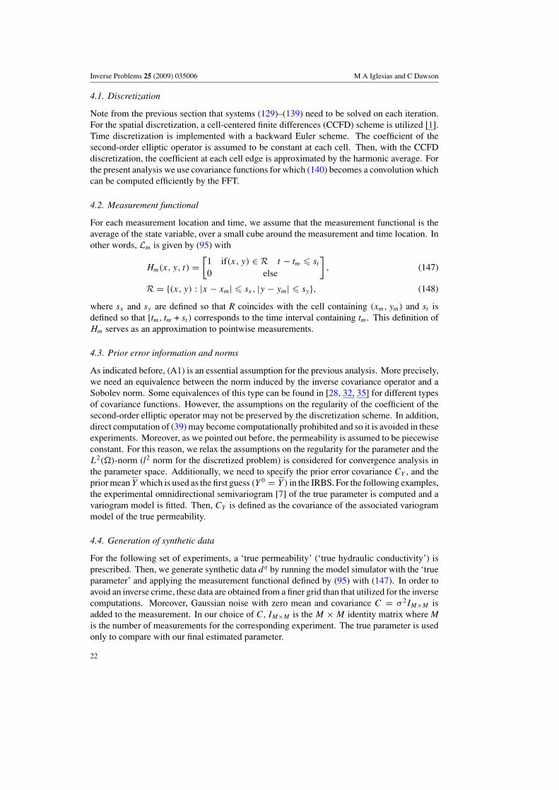
4.1. Discretization

Note from the previous section that systems (129)–(139) need to be solved on each iteration.For the spatial discretization, a cell-centered finite differences (CCFD) scheme is utilized [1].Time discretization is implemented with a backward Euler scheme. The coefficient of thesecond-order elliptic operator is assumed to be constant at each cell. Then, with the CCFDdiscretization, the coefficient at each cell edge is approximated by the harmonic average. Forthe present analysis we use covariance functions for which (140) becomes a convolution whichcan be computed efficiently by the FFT.

4.2. Measurement functional

For each measurement location and time, we assume that the measurement functional is theaverage of the state variable, over a small cube around the measurement and time location. Inother words, Lm is given by (95) with

Hm(x, y, t) =[

1 if(x, y) ∈ R t − tm � st

0 else

], (147)

R = {(x, y) : |x − xm| � sx, |y − ym| � sy}, (148)

where sx and sy are defined so that R coincides with the cell containing (xm, ym) and st isdefined so that [tm, tm + st ) corresponds to the time interval containing tm. This definition ofHm serves as an approximation to pointwise measurements.

4.3. Prior error information and norms

As indicated before, (A1) is an essential assumption for the previous analysis. More precisely,we need an equivalence between the norm induced by the inverse covariance operator and aSobolev norm. Some equivalences of this type can be found in [28, 32, 35] for different typesof covariance functions. However, the assumptions on the regularity of the coefficient of thesecond-order elliptic operator may not be preserved by the discretization scheme. In addition,direct computation of (39) may become computationally prohibited and so it is avoided in theseexperiments. Moreover, as we pointed out before, the permeability is assumed to be piecewiseconstant. For this reason, we relax the assumptions on the regularity for the parameter and theL2(�)-norm (l2 norm for the discretized problem) is considered for convergence analysis inthe parameter space. Additionally, we need to specify the prior error covariance CY , and theprior mean Y which is used as the first guess (Y 0 = Y ) in the IRBS. For the following examples,the experimental omnidirectional semivariogram [7] of the true parameter is computed and avariogram model is fitted. Then, CY is defined as the covariance of the associated variogrammodel of the true permeability.

4.4. Generation of synthetic data

For the following set of experiments, a ‘true permeability’ (‘true hydraulic conductivity’) isprescribed. Then, we generate synthetic data dη by running the model simulator with the ‘trueparameter’ and applying the measurement functional defined by (95) with (147). In order toavoid an inverse crime, these data are obtained from a finer grid than that utilized for the inversecomputations. Moreover, Gaussian noise with zero mean and covariance C = σ 2IM×M isadded to the measurement. In our choice of C, IM×M is the M × M identity matrix where Mis the number of measurements for the corresponding experiment. The true parameter is usedonly to compare with our final estimated parameter.

22

Inverse Problems 25 (2009) 035006 M A Iglesias and C Dawson

4.5. Stopping rule

The stopping criteria for the algorithm presented in section 2 requires an estimate of the noiselevel. However, only the measurements (dη) as well as the prior error statistics (σ ) may beavailable. To obtain an estimate of the error level in the case C = σ 2I , we assume thatdη = d + σe where e is a Gaussian random variable with zero mean and variance equalsone. Therefore, since dη − d = σe, if we assume that |ej | � 1, it follows ‖dη − d‖2

C−1 =∑Mj

1σ 2

∣∣dη

j − dj

∣∣2 = ∑Mj |ej |2 � M . Thus, ‖dη − d‖C−1 �

√M . With this argument we

propose to use η = √M as the noise level for the algorithm. For the stopping criteria, we

recall that the IRBS is terminated when∥∥dη − L

(snF

)∥∥C−1 � τ

√M for the first time. Having

discussed some general considerations, we now introduce some examples. The objective ofthese experiments is to analyze the efficiency of the IRBS to obtain improved parameters whilefitting the synthetic data.

4.6. The groundwater flow

Groundwater flow can be modeled by the following equation [5]:

S∂h

∂t− ∇ · eY ∇h = f, (149)

where S is specific storage, f accounts for sources, eY is the hydraulic conductivity and h isthe piezometric head. When proper boundary conditions are imposed, (149) takes the form(up to known constants) of the operator (34). The parameter to be estimated is Y and all theother parameters are assumed to be perfectly known.

4.6.1. Experiment I. In order to validate the IRBS presented in the previous sections, weconsider the same problem used in [19]. The forward model is the steady state of (149) overa square domain of dimension 6 km × 6 km. The boundary conditions are given by

u(x, 0) = 100 m, ux(6 km, y) = 0, (150)

−eY ux(0, y) = 500 m3 km−1 day−1, uy(x, 6 km) = 0 (151)

and a constant (in time) recharge is represented by

f (x, y) =

⎧⎪⎨⎪⎩

0 0 < y < 4 km,

0.137 × 10−3m d−1 4 km < y < 5 km,

0.274 × 10−3 m d−1 5 km < y < 6 km.

(152)

The grid used for the synthetic data generation and for the IRBS are 180 × 180 and 60 × 60respectively. The measurement locations are shown in figure 1(a). For the prior mean ofY = ln K we select the natural logarithm of the initial guess used in [19]. Note from figure 1(b),that the true conductivity is anisotropic and therefore, the omnidirectional semivariogramis poor prior knowledge of the truth. It is the purpose of this example to illustrate theefficiency of our method when limited information is provided. The covariance associatedwith the variogram model fitted to the experimental semivariogram as well as other pertinentinformation are displayed in table 1. In Experiments IA and IB we follow [19] and test thescheme for two different signals-to-noise ratios (SNR). The estimated results are displayed infigure 1(c) and (d) where a good agreement to the true log hydraulic conductivity is obtained.Figure 1(e) shows the true and estimated hydraulic conductivity fields projected along thephantom shown in figure 1(a) (dotted red line). Convergence history for IA and IB are

23

Inverse Problems 25 (2009) 035006 M A Iglesias and C Dawson

0 1 2 3 4 5 60

1

2

3

4

5

6

X (km)

Y(k

m)

50

150

50

15

15

5

(a)

(c) (d)

(b)

0 1 2 3 4 5 60

1

2

3

4

5

6

x (km)

y (

km

)

1

1.5

2

2.5

3

3.5

4

4.5

5

5.5

0 1 2 3 4 5 60

1

2

3

4

5

6

x (km)

y (

km

)

1

1.5

2

2.5

3

3.5

4

4.5

5

5.5

0 1 2 3 4 5 6 70

20

40

60

80

100

120

140

160

180

200

Distance (km)

K (

m/d

ay)

True

Exp IA

Exp IB

(e)

Figure 1. Experiment I. Top left: aquifer configuration (observation wells are indicated by *). Topright and middle: log hydraulic conductivity fields [ln (md−1)]. Bottom: hydraulic conductivity(m d−1) fields projected over the phantom. (a) Configuration, (b) true, (c) experiment IA, (d)experiment IB and (e) phantom.

displayed in table 2. Note that for smaller (SNR), the IRBS provides smaller error in thecomputed parameter. In contrast to the work in [19] where the hydraulic conductivity K isidentified, in our approach the estimation is performed for Y = ln K . Although the latter

24

Inverse Problems 25 (2009) 035006 M A Iglesias and C Dawson

Table 1. Information for data assimilation. Experiment I.

Experiment IA IB

Number of measurement locations 18 18τ 1.5 1.5ητ (m) 6.3640 6.3640σ (m) 1.8 0.18Y [ln md−1] ln 20 ln 20

CY (ξ, ξ ′)[ln(m d−1)]2 2.2 exp[− ‖ξ−ξ ′‖

1 km

]2.2 exp

[− ‖ξ−ξ ′‖

1 km

]Signal-to-noise ratio 102.27 1034

Table 2. Numerical results. Experiment I.

Experiment IA Experiment IB

n ‖Yn−1 − Ytrue‖l2 ‖dη − L(pnF )‖C−1 ‖Yn−1 − Ytrue‖l2 ‖dη − L(pn

F )‖C−1

1 178.9116 227.729 178.9116 2280.3192 114.0224 69.773 116.4194 692.8733 81.7970 15.274 83.2218 138.3254 70.4071 2.082 69.2700 13.5385 – – 67.839 0.381

approach imposes a stronger nonlinearity in the abstract formulation, the implementation doesnot require modification when negative values of the parameter occur. This may become anadvantage in problems (see experiment III) where the true parameter changes by several ordersof magnitude, and further modifications may be detrimental to the quality of the identification.

We remark that the measurement data are assimilated only from the measurementlocations. Unlike the standard parameter identification approaches, there is no need tointerpolate the entire field of the state variable. Moreover, Hanke [19] reported that whenthe parameter identification problem is posed with a finite-dimensional measurement space,their method becomes considerably less efficient. On the other hand, the IRBS convergence isachieved in a few iterations with satisfactory results. Such behavior should not be surprisingsince the present approach takes into account prior information.

4.7. The single-phase Darcy flow through porous media

We now study the reservoir model described by (1).

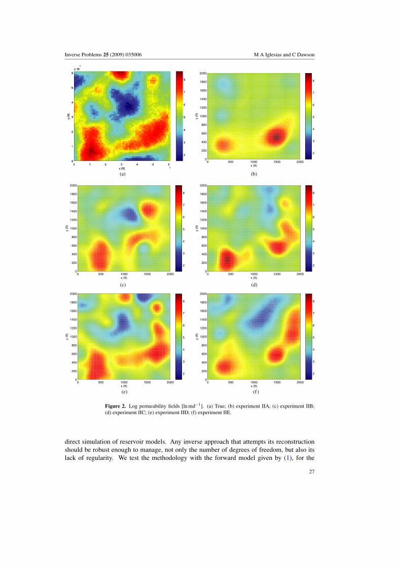
4.7.1. Experiment II. In experiment II we are interested in determining the efficiency forthe estimation of the log permeability Y = ln K from pressure data collected at differentconfigurations. The true log permeability (figure 2(a)) is generated stochastically with theroutine SGSIM [7]. Table 3 shows the reservoir properties and table 4 presents prior errorinformation. Table 5 provides the corresponding information for each run whose correspondingestimations are presented in figures 2(b)–(f). For experiments IIB, IIC and IID, the observationwells are equally spaced over the domain but they do not coincide with either the injection orthe production wells. For experiments IIA and IIE measurements are collected at the injectionand production wells. It comes as no surprise that the quality of the reconstruction dependson the number of measurements available. However, the measurement locations also affect

25

Inverse Problems 25 (2009) 035006 M A Iglesias and C Dawson

Table 3. Reservoir description. Experiments II and III.

Experiment II III

Dimension (ft3) 2000 × 2000 × 2 2000 × 4000 × 2Grid blocks (for synthetic data) 180 × 180 × 1 60 × 220 × 1Grid blocks (for IRBS) 60 × 60 × 1 60 × 110 × 1Time interval [0, T ] (day) [0,1] [0, 1]Time discretization dt (day) 0.01 0.01Porosity 0.2 0.2Water compressibility (psi−1) 3.1 ×10−6 3.1×10−6

Rock compressibility (psi−1) 1.0×10−6 1.0 ×10−6

Water viscosity (cp) 0.3 0.3Initial pressure (psi) 5000 10 000Number injection wells 2 4Number production wells 6 5Shut-in time ts (day) 0.75 0.75Injection ratea (stb d−1) 2500 1000Production ratea (stb d−1) 833.33 1000

a Rate per well in the interval [0, ts ].

Table 4. Prior error information for experiment II.

τ 2.0σ (psi) 5.0Y (ln md) 196.42

CY (ξ, ξ ′) (ln(md))2 0.95 exp[− ‖ξ−ξ ′‖

400 ft

]

Table 5. Numerical results. Experiment II.

Configuration IIA IIB IIC IID IIE

Number of measured location 8 16 25 36 8Number of measured times 1 1 1 1 2τη[psi] 5.6569 8 10.00 12.00 8.00

‖Ytrue − Y ∗‖a,bl2

[ln(md)] 68.74 63.75 58.08 47.27 59.84

Iterations 5 3 4 4 6

a Y ∗ ≡ lim Yn.b ‖Y − Ytrue‖l2 = 79.19.

the final outcome. It is also worth mentioning that the best estimate of log permeability wasobtained with experiment IIE which corresponds to the configuration of maximum numberof observation wells. Additionally, convergence is achieved within the first five iterations forall the different configurations. Clearly, non-uniqueness is always evident since for a smallnumber of observations, there are many possible parameters that will fit the data.

4.7.2. Experiment III: SPE model. In experiment III we are interested in the estimationof a more realistic permeability field. The true permeability (figure 3(a)) is taken from thethird layer of the absolute permeability data for the 10th SPE comparative project [20]. Oneof the interesting aspects of this permeability is that it has a variability of several orders ofmagnitude (10−3–104 md). A heterogeneous field of this type is challenging even for the

26

Inverse Problems 25 (2009) 035006 M A Iglesias and C Dawson

(a)

0 500 1000 1500 20000

200

400

600

800

1000

1200

1400

1600

1800

2000

x (ft)

y (

ft)

2

3

4

5

6

7

8

(b)

0 500 1000 1500 20000

200

400

600

800

1000

1200

1400

1600

1800

2000

x (ft)

y (

ft)

2

3

4

5

6

7

8

(c)

0 500 1000 1500 20000

200

400

600

800

1000

1200

1400

1600

1800

2000

x (ft)

y (

ft)

2

3

4

5

6

7

8

(d)

0 500 1000 1500 20000

200

400

600

800

1000

1200

1400

1600

1800

2000

x (ft)

y (

ft)

2

3

4

5

6

7

8

(e)

0 500 1000 1500 20000

200

400

600

800

1000

1200

1400

1600

1800

2000

x (ft)

y (

ft)

2

3

4

5

6

7

8

(f )

Figure 2. Log permeability fields [ln md−1]. (a) True; (b) experiment IIA; (c) experiment IIB;(d) experiment IIC; (e) experiment IID; (f) experiment IIE.

direct simulation of reservoir models. Any inverse approach that attempts its reconstructionshould be robust enough to manage, not only the number of degrees of freedom, but also itslack of regularity. We test the methodology with the forward model given by (1), for the

27

Inverse Problems 25 (2009) 035006 M A Iglesias and C Dawson

0 500 1000 1500 20000

500

1000

1500

2000

2500

3000

3500

4000

x (ft)

y (

ft)

0

5

10

(a)

0 500 1000 1500 20000

500

1000

1500

2000

2500

3000

3500

4000

x (ft)

y (

ft)

0

5

10

(b)

0 500 1000 1500 20000

500

1000

1500

2000

2500

3000

3500

4000

x (ft)

y (

ft)

0

5

10

(c)

Figure 3. Log permeability fields. (a) True; (b) experiment IIIA; (c) experiment IIIB [ln md].

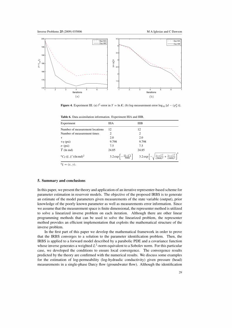
estimation of the permeability from synthetic data (pressure). Measurements are collected atthe injection and production wells, as wells as two additional observation wells. Table 3 showsthe reservoir description and table 6 presents the information for the assimilation experiments.Figures 4(a) and (b) show the convergence history for both experiments. From figure 3(a) itis clear that the true log permeability is anisotropic. Although the isotropic covariance is onlypoor prior knowledge of the spatial variability, the estimated log permeability in figure 3(b)captures some of the main characteristics of the true log permeability field. In experiment IIIBwe select, by inspection, a different error covariance function that reflects the higher spatialcorrelation in the x-direction. According to the definition of noise level (section 4.5), bothexperiments have the same stopping threshold. In fact, from figure 4(d) it can be observedthat data have been fitted with about the same accuracy. However, in experiment IIIB, animproved estimation is achieved (figure 3(c)) because we considered ‘better’ prior knowledge(correlation lengths) than in experiment IIIA.

28

Inverse Problems 25 (2009) 035006 M A Iglesias and C Dawson

1 2 3 4 5 6 7170

175

180

185

190

195

200

Iterations

tru

e||

l2

Exp IIIA

Exp IIIB

1 2 3 4 5 6 71

1.5

2

2.5

3

3.5

4

4.5

Iterations

Fn)|

|

Exp IIIA

Exp IIIB

Figure 4. Experiment III. (a) l2-error in Y = ln K; (b) log-measurement error log10 ‖d − (pnF )‖.

Table 6. Data assimilation information. Experiment IIIA and IIIB.

Experiment IIIA IIIB

Number of measurement locations 12 12Number of measurement times 2 2τ 2.0 2.0τη (psi) 9.798 9.798σ (psi) 7.5 7.5Y (ln md) 24.85 24.85

aCY (ξ, ξ ′)(ln md)2 3.2 exp[− ‖ξ−ξ ′‖

500ft

]3.2 exp

[−√

|x−x′ |2(286ft)2 + |y−y′ |2

(160ft)2

]a

aξ = (x, y).

5. Summary and conclusions

In this paper, we present the theory and application of an iterative representer-based scheme forparameter estimation in reservoir models. The objective of the proposed IRBS is to generatean estimate of the model parameters given measurements of the state variable (output), priorknowledge of the poorly known parameter as well as measurements error information. Sincewe assume that the measurement space is finite dimensional, the representer method is utilizedto solve a linearized inverse problem on each iteration. Although there are other linearprogramming methods that can be used to solve the linearized problem, the representermethod provides an efficient implementation that exploits the mathematical structure of theinverse problem.

In the first part of this paper we develop the mathematical framework in order to provethat the IRBS converges to a solution to the parameter identification problem. Then, theIRBS is applied to a forward model described by a parabolic PDE and a covariance functionwhose inverse generates a weighted L2-norm equivalent to a Sobolev norm. For this particularcase, we developed the conditions to ensure local convergence. The convergence resultspredicted by the theory are confirmed with the numerical results. We discuss some examplesfor the estimation of log-permeability (log-hydraulic conductivity) given pressure (head)measurements in a single-phase Darcy flow (groundwater flow). Although the identification

29

Inverse Problems 25 (2009) 035006 M A Iglesias and C Dawson

problem is ill-posed, the iterative scheme has been proved to be robust enough to generateimproved parameters while fitting the data. Stability was obtained when different signal-to-noise ratios are compared in experiment I.

In contrast to the classical parameter identification approach, our approach assumes someprior knowledge of the uncertain parameter. However, our numerical results show that evenwith poor prior knowledge, the reconstructions capture the main heterogeneities of the fields.Moreover, when large problems and highly heterogenous fields are considered (experimentIII), the IRBS generates improved parameters in a stable fashion. It is worth mentioning thatthe IRBS possesses an interesting flexibility for more general applications. The theory isapplicable to the simultaneous estimation of reservoir properties. Furthermore, since time-dependent parameters can also be estimated, ‘model error’ can be allowed in the formulationas in [6, 21, 33]. In addition, any reservoir model can be used with this theory as long ashypotheses (F1)–(F4) are satisfied.

The numerical results are promising and indicate that the IRBS may become a tool forparameter estimation in reservoir modeling. With the integration of seismic data and smart-wells technology, better prior knowledge and reliable measurements may result in an improvedreservoir characterization. Future comparison with the state-of-the-art methodologies must beconducted.

Acknowledgment

This research was supported in part by NSF grant DMS-0411413.

Appendix

The proof of theorem 2.2 is very similar to the proof of theorem 2.2 [19]. Therefore, onlysome technical differences and equivalences are pointed out. First, we need the following

Lemma A.1. Let d∗ ∈ RM and C ∈ R

M×M a positive-definite matrix. Suppose assumption(A1) and (F1)–(F3) hold. For any k∗ ∈ K and r > 0, let C1 be the constant in (F3) for theclosed ball B(r, k∗). Define ρ as in (32) Suppose that for some n, the following inequality issatisfied

‖dη − L(sr )‖C−1 � ρ

κ

∥∥dη − L(snF

)∥∥C−1 (A.1)

for some κ > 1, where sr is the solution to

DkG(kn−1, sn

F

)[k∗ − kn−1] + DsG

(kn−1, sn

F

)[sr − sn

F

] = 0. (A.2)

If kn−1 ∈ B(r, k∗), then kn defined by (24) for dη = d∗ satisfies

‖k∗ − kn−1‖2K − ‖k∗ − kn‖2

K > 2ρ2

[κ − 1

κ

]∥∥d∗ − L(snF

)∥∥2C−1 . (A.3)

Proof. First we note that the assumptions on theorem 2.1 are satisfied. Then, kn is well definedin terms of (24). Let, s∗ be the solution to G(k∗, s∗) = 0. Since G satisfies (F1)–(F3), by theimplicit function theorem (IFT), there exists a neighborhood U of k∗ such that G(k, s(k)) = 0for all k ∈ U , where s : U → S is a continuous function. Let us define the nonlinear operatorF : K → R

M by F(k) = (L ◦ s)(k), and consider the weighted norm in RM by C. From

hypothesis (F2), F is continuous. Consider now T = F ′(kn−1). Note that if kn−1 ∈ B(r, k∗), by(F3) it follows that ‖T ‖ � ‖L‖C1 and so T is locally bounded. Then F satisfies the hypothesesused in [19]. On the other hand, from the definition of sr (A.2) and the invertibility of

30

Inverse Problems 25 (2009) 035006 M A Iglesias and C Dawson

DsG(kn−1, sn−1

F

)it follows that sr = sn

F − [DsG

(kn−1, sn−1

F

)]−1DkG

(kn−1, sn−1

F

)[k∗ − kn−1].

Therefore, (A.1) is equivalent to

‖uη − F(kn−1) − F ′(kn−1)[k∗ − kn−1]‖= ∥∥dη − L

(snF

) − L ◦ DsGDkG[k∗ − kn−1]∥∥

C−1

� ρ

κ

∥∥dη − L(snF

)∥∥C−1 = ρ

κ‖uη − F(kn−1)‖ (A.4)

which is condition (2.1) in [19]. Then we can apply the same argument that yields (2.16) in[19] to conclude that

‖k∗ − kn−1‖2K − ‖k∗ − kn‖2

K

> 2∥∥AC−1/2[d∗ − L

(snF

)]∥∥[∥∥AC−1/2[d∗ − L(snF

)]∥∥ − ρ

κ

∥∥d∗ − L(snF

)∥∥C−1

](A.5)

for A = [C−1/2RnC−1/2 + I ]−1. In contrast to the work of [19], the first term on the right-handside of (14) is weighted by C−1. For this reason C−1/2 appears in (A.5) after the appropriatefactorization. From the definition of A, estimate (20) and (32) it follows that∥∥AC−1/2[d∗ − L

(snF

)]∥∥ � 1

‖A−1‖∥∥d∗ − L

(snF

)∥∥C−1

� 1

‖C−1‖C21‖L‖2 + 1

∥∥d∗ − L(snF

)∥∥C−1 = ρ

∥∥d∗ − L(snF

)∥∥C−1 . (A.6)

This is substituted into (A.5) to obtain

‖k∗ − kn−1‖2K − ‖k∗ − kn‖2

K

> 2ρ∥∥d∗ − L

(snF

)∥∥C−1

[ρ∥∥d∗ − L

(snF

)∥∥C−1 − ρ

κ

∥∥d∗ − L(snF

)∥∥C−1

]

from which (A.3) follows. �

Before we discuss the proof of theorem 2.2, we need the result for the idealized case of perfectmeasurements.

Theorem A.1. Let d ∈ RM be the vector of exact measurements and C ∈ R

M×M an arbitrarypositive-definite matrix with eigenvalues {λi}Mi=1 and α ≡ max λi/ min λi . Let us assume (A1)and (F1)–(F4) and let k∗ be a solution to the PIP. For k = k∗, take C2 and δ > 0 as in (F4).Consider B(δ/2, k∗) and the corresponding constant C1 as in (F3). Let ρ be defined by (32).If k0 = k (the initial guess) satisfies

‖k∗ − k‖K < min

{δ

2, κ2

}(A.7)

for some κ2 <ρ

2C2α1/2 , then kn, defined in (24) for dη = d∗, converges to a solution to the PIP.

Proof. By showing an analogous inequality to (A.4) for κ = ρ/(C2α1/2κ2), the proof is

carried out exactly as in [19] except for the use of (A.3). �

Proof of theorem 2.2. Assume η > 0 is fixed. Let s1r be the solution to

DsG(k0, s1

F

)[s1r − s∗

] = Gr

(s∗ − s1

F , k∗ − k). (A.8)

31

Inverse Problems 25 (2009) 035006 M A Iglesias and C Dawson

Since ‖k∗ − k‖K � δ/2 < δ, we apply (F4) (for k = k = k∗ and k = k) to obtain∥∥L(s∗) − L(s1r

)∥∥ � C2‖k∗ − k‖K∥∥L(s∗) − L

(s1F

)∥∥. (A.9)

Then, it is not difficult to show that∥∥L(s∗) − L(s1r

)∥∥C−1 � ‖C−1‖1/2

∥∥L(s∗) − L(s1r

)∥∥� ‖C−1‖1/2C2‖k∗ − k‖K

∥∥L(s∗) − L(s1F

)∥∥� α1/2C2‖k∗ − k‖K

∥∥L(s∗) − L(s1F

)∥∥C−1 . (A.10)

Therefore, the same steps of [19] can be used to find∥∥dη − L(s1r

)∥∥C−1 � ρ

κ‖k∗ − k0‖K

∥∥dη − L(s1F

)∥∥C−1 (A.11)

for

κ = ρτ

1 + (1 + τ)C2α1/2‖k∗ − k0‖K . (A.12)

Then, since k ∈ B(δ/2, k∗) we may apply lemma A.1 to obtain that k1η , defined by (24),

satisfies

‖k∗ − k0‖2K − ∥∥k∗ − k1

η

∥∥2K > 2ρ2

[κ − 1

κ

]∥∥dη − L(s1F

)∥∥2C−1 (A.13)

(we have added the subscript η to emphasize that k1η depends on this case of dη). From (A.12)

it is clear that κ > 1 which implies δ/2 > ‖k∗ − k‖2K >

∥∥k∗ − k1η

∥∥2K. By applying this

methodology inductively, we show that knη given by (24) satisfies

∥∥k∗ − kn−1η

∥∥2K >

∥∥k∗ − knη

∥∥2K (A.14)

as long as τη <∥∥dη − L

(smF

)∥∥C−1 and so the sequence kn

η is monotone decreasing. Let usassume that for n = n(η),∥∥dη − L

(snF

)∥∥C−1 � τη. (A.15)

From (A.13) it follows that

n(η)−1∑n=1

(∥∥k∗ − kn−1η

∥∥2K − ∥∥k∗ − kn

η

∥∥2K)

> 2ρ2

[κ − 1

κ

] n(η)−1∑n=1

∥∥dη − L(snF

)∥∥2C−1 . (A.16)

Reducing some terms on the left-hand side and using the fact that τη <∥∥dη − L

(snF

)∥∥C−1 we

find

∞ > ‖k∗ − k‖2K � ‖k∗ − k‖2

K − ∥∥k∗ − kn(η)−1η

∥∥2K > 2ρ2

[κ − 1

κ

]τ 2η2(n(η) − 1).

This inequality shows that, given η > 0 fixed, the discrepancy principle terminates the IRBSafter a finite number n(η) of iterations. We now observe from (33) that theorem A.1 can beapplied where now Kn is the sequence given by (24) with dη replaced by d. We now pointout to the fact that for theorem 2.2 in [19], the current estimate kn is related to the choice ofthe Levenberg–Marquardt parameter αk . In our approach this parameter is fixed (αk = 1) andthe current estimate kn is computed from (24). However, with our selection of kn, the proof is

32

Inverse Problems 25 (2009) 035006 M A Iglesias and C Dawson

still valid since from (24) it is easy to see that

knη − Kn = kn−1

η − Kn−1 + [γ n(ξ)]T [Rn + C]−1[dη − d]

+ [γ n(ξ)]T [Rn + C]−1[L(snF

) − L(snF,η

)], (A.17)

where snF is the solution to G(Kn−1, sn

F ) = 0. With an inductive argument and using theuniform bounds for γ n and Rn (see (21)–(23)) it follows that kn

η → Kn as η → 0. Therefore,from (A.15) it follows that as η → 0,L

(snF

) = d for n(δ) finite, which implies that kn(η)η

converges to Kn which in turn is a solution to the PIP. The proof when n → ∞ can beconducted as in [19]. �

References

[1] Arbogast T, Wheeler M F and Yotov I 1997 Mixed finite elements for elliptic problems with tensor coefficientsas cell-centered finite differences SIAM J. Numer. Anal. 34 828–52

[2] Baird J and Dawson C 2005 The representer method for data assimilation in single-phase Darcy flow in porousmedia Comput. Geosci. 9 (4) 247–71 (doi:10.1007/s10596-005-9006-2)

[3] Baird J and Dawson C 2007 The representer method for two-phase flow in porous media Comput.Geosci. 11 (3) 235–48 (doi:10.1007/s10596-007-9048-8)

[4] Baird J and Dawson C 2007 A posteriori error estimation of the representer method for single phase Darcy flowComput. Methods Appl. Mech. Eng. 196 1623–32

[5] Bear J 1972 Dynamics of Fluids in Porous Media (New York: Dover)[6] Bennett A F 2002 Inverse Modeling of the Ocean and Atmosphere (Cambridge: Cambridge University Press)[7] Deutsch C V and Journel A G 1997 GSLIB: Geostatistical Software Library 2nd edn (New York: Oxford

University Press)[8] Dimet F Le and Talagrand O 1986 Variational algorithms for analysis and assimilation of meteorological

observations Tellus 38A 97–110[9] Dong Y, Gu Y and Oliver D S 2006 Sequential assimilation of 4D seismic data for reservoir description using

the Ensemble Kalman Filter J. Pet. Sci. Eng. 53 83–99[10] Engl H W, Hanke M and Neubauer A 1996 Regularization of Inverse Problems 1st edn (Dordrecht: Kluwer)[11] Evans L C 1998 Partial Differential Equations 1st edn (Providence, RI: American Mathematical Society)[12] Evensen G 1994 Sequential data assimilation with a non-linear quasi-geostrophic model using Monte-Carlo

methods to forecast error statistics J. Geophys. Res. 99 10143–62[13] Evensen G 2007 Data Assimilation 1st edn (Heidelberg: Springer)[14] Evensen G, Hove J, Meisingset H C, Reiso E and Seim K S 2007 Using the EnKF for assisted history matching

of a North Sea reservoir model SPE Reservoir Simulation Symp. (Woodlands, TX, 26–28 February 2007,SPE 106184)

[15] Gao C, Rajeswaran T and Nakagawa E 2007 A literature review on smart-well technology Proc. SPE Productionand Operations Symp. (Oklahoma City, OK, 31 March–3 April 2007, SPE 106011)

[16] Giudici M 1991 Identifiability of distributed physical parameters in diffusive-like systems Inverse Problems7 231–45

[17] Gu Y and Oliver D S 2005 History matching of the PUNQ-S3 reservoir model using the Ensemble KalmanFilter SPE J. 10 51–65

[18] Gu Y and Oliver D S 2006 The ensemble Kalman filter for continuous updating of reservoir simulation modelsJ. Energy Resour. Technol. 128 79–87

[19] Hanke M 1997 A regularizing Levenberg–Marquardt scheme, with applications to inverse groundwater filtrationproblems Inverse Problems 13 79–95

[20] http://www.spe.org/csp/ (Spe 10th comparative project)[21] Iglesias M A and Dawson C 2007 The representer method for state and parameter estimation in single-phase

Darcy flow Comput. Methods Appl. Mech. Eng. 196 4577–96[22] Kalman R E 1960 A new approach to linear filtering and prediction problems Trans. ASME J. Basic Eng.

82 35–45[23] Lions J L and Magenes E 1972 Non-Homogeneous Boundary Value Problems and Applications vol II (Berlin:

Springer)[24] Liu N and Oliver D S 2005 Ensemble Kalman filter for automatic history matching of geologic facies J. Pet.

Sci. Eng. 47 147–61

33

Inverse Problems 25 (2009) 035006 M A Iglesias and C Dawson

[25] Lorentzen R J, Naevdal G, Valls B and Berg A M 2005 Analysis of the ensemble Kalman filter for estimationof permeability and porosity in reservoir models SPE Annual Technical Conf. and Exhibition (Dallas, TX,9–12 October 2005, SPE 96375)

[26] Naevdal G, Johnsen L M, Aanonsen S I and Vefring E H 2005 Reservoir monitoring and continuous modelupdating using ensemble Kalman filter SPE J. 10 66–74

[27] Naevdal G, Mannseth T and Vefring E H 2002 Near-well reservoir monitoring through ensemble Kalman filterSEP/DOE Improved Oil Recovery Symp. (Tulsa, OK, April 2002, SPE 75235)

[28] Oliver D S 1998 Calculation of the inverse of the covariance Math. Geol. 30 911–33[29] Przybysz-Jarnut J K, Hanea R G, Jansen J D and Heemink A W 2007 Application of the representer method for

parameter estimation in numerical reservoir models Comput. Geosci. 11 73–85[30] Rosmond T and Xu L 2006 Development of NAVDAS-AR: non-linear formulation and outer loop test Tellus

A 58 45–58[31] Skjervheim J A, Evensen G, Aanonsen S I, Ruud B O and Johansen T A 2005 Incorporating 4d seismic data

in reservoir simulation models using Ensemble kalman filter SPE Annual Technical Conf. and Exhibition(Dallas, TX, 9–12 October 2005, SPE 95789)

[32] Tarantola A 1987 Inverse Problems Theory: Methods for Data Fitting and Model Parameter Estimation 1st edn(New York: Elsevier)

[33] Valstar J R, McLaughlin D B, te Stroet C B M and van Geer F C 2004 A representer-based inverse method forgroundwater flow and transport applications Water Resour. Res. 40 W05116 (doi:10.1029/2003WR002922)

[34] Xu L and Daley R 2000 Towards a true 4-dimensional data assimilation algorithm: application of a cyclingrepresenter algorithm to a simple transport problem Tellus 52A 109–28

[35] Xu Q 2005 Representation of inverse covariance by differential operators Adv. Atmos. Sci. 22 181–98

34